Individual Tree Taper, Volume and Weightfor Loblolly Pine

Bruce E. BordersWestern MensurationistsFortuna, CAJune 18-20, 2006

Current Models

Compatible total/merchantable tree volume/weight/taper functions

Fitted separately by physiographic region (LCP, UCP, Piedmont)

Large number of sample trees used in fit – however the range of data is limited in stem size (approximately 1500 trees largest DBH = 14” class)

Problems using ratios low on the stem Implied Taper functions not very realistic (taper

function derived from ratio volume equation)

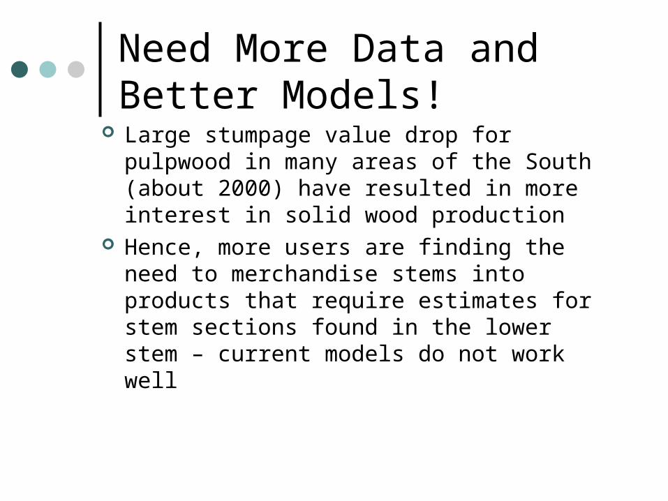
Need More Data and Better Models!

Large stumpage value drop for pulpwood in many areas of the South (about 2000) have resulted in more interest in solid wood production

Hence, more users are finding the need to merchandise stems into products that require estimates for stem sections found in the lower stem – current models do not work well

Other Data Sources CAPPS Destructively Sampled Trees

Age 6, 10, 12 years – data will be added to PMRC individual tree database

Wood Quality Consortium Destructively Sampled Trees – 272 trees distributed across southern U.S.

U.S. Forest Service – FIA unit has a relatively large database with volume, weight and taper information available

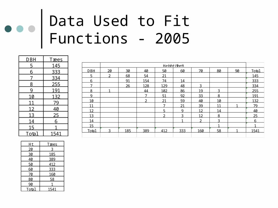
Data Used to Fit Functions - 2005

DBH Trees5 1456 3337 3348 2559 191

10 13211 7912 4013 2514 615 1

Total 1541

Ht Trees20 330 18540 38950 41260 33370 16080 5890 1

Total 1541

DBH 20 30 40 50 60 70 80 90 Total5 2 68 54 21 1456 91 154 74 14 3337 26 128 129 48 3 3348 1 44 102 86 19 3 2559 7 51 92 33 8 19110 2 21 59 40 10 13211 7 21 39 11 1 7912 5 9 12 14 4013 2 3 12 8 2514 1 2 3 615 1 1

Total 3 185 389 412 333 160 58 1 1541

Height (feet)

Data Used to Test Functions - 2005

DBH Trees5 256 877 868 769 5110 4311 4012 1813 1114 115 1016 3

Total 451

Ht Trees20 030 1240 7350 16960 11770 6080 1690 4

Total 451

DBH 20 30 40 50 60 70 80 90 Total5 3 16 6 256 9 31 42 5 877 16 53 15 2 868 8 38 25 4 1 769 1 16 24 9 1 5110 1 7 24 11 4311 5 14 18 3 4012 2 5 5 5 1 1813 4 5 2 1114 1 115 1 4 2 3 1016 1 2 3

Total 0 12 73 169 117 59 14 4 451

Height (feet)

NOTE – all data will be combined for final model fits

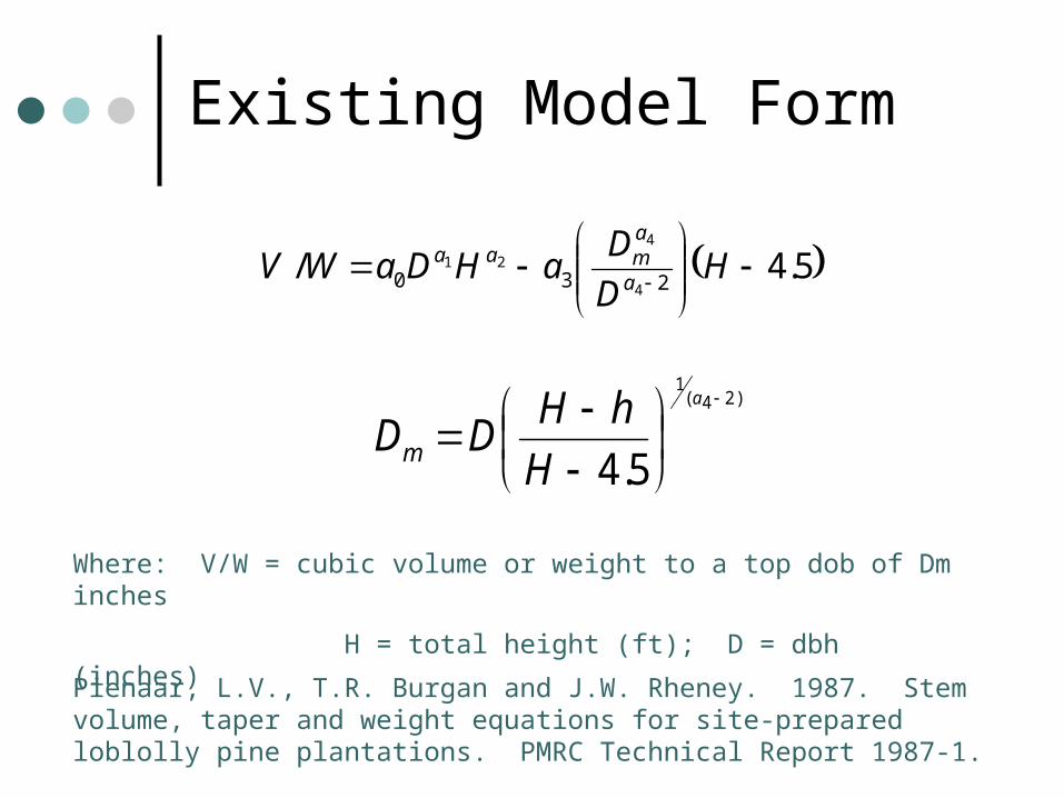
Existing Model Form

5.4/ 230 4

4

21

H

D

DaHDaWV a

amaa

)24(1

5.4

a

H

hHDDm

Where: V/W = cubic volume or weight to a top dob of Dm inches

H = total height (ft); D = dbh (inches)

Pienaar, L.V., T.R. Burgan and J.W. Rheney. 1987. Stem volume, taper and weight equations for site-prepared loblolly pine plantations. PMRC Technical Report 1987-1.

Existing Model Forms

Simple models – a lot of appeal for ease of use

Models fitted separately by LCP, UCP, Piedmont

Predict cubic volume inside/outside bark Predict green weight inside/outside bark Predict dry weight with and without bark

Existing Model Forms

These models were developed for use in estimating volume or weight to a given top diameter

However, the model form has limited flexibility in reflecting stem form realistically and it was fitted by Pienaar et al. (1987) with data bases structured to have Dm values of 6” and smaller

Today – users require capability to merchandise stems into various products that may be found anywhere within the stem

Existing Model Form

NOTE – the functions did not perform any better when fitted to the new database

New Functions – Taper/Volume

Objective – provide two sets of functions1. Simple and easy to implement (e.g. a ratio volume/weight

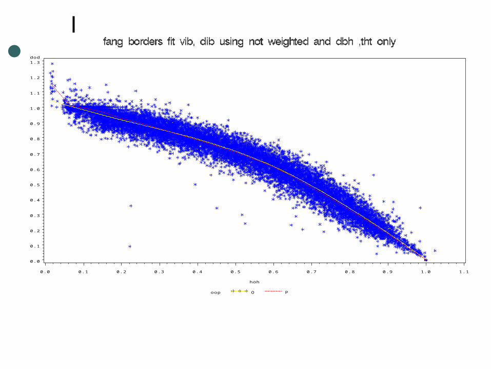
equation and associated taper function) – realize that weaknesses will exist – fitted and evaluated model forms suggested by Bailey (1994), Zhang et al. (2002) and Fang et al. (2000) – only present results for Fang (2000) model

2. Sophisticated and very flexible system that should provide very accurate estimates of stem volume and weight for any stem segment – realize that implementation will require thorough understanding of the functions to be programmed (based on work of Clark, A. III, R.A. Souter and B. Schlaegel. 1991)

New Functions - Weight

1. Weights will be predicted using a per cubic foot density measure (lbs of wood and bark per cubic foot of wood)

2. Thus, to determine the green weight of wood and bark in any specific stem section we will calculate the cubic foot volume of wood and multiply by lbs of wood and bark per cubic foot of wood

3. These densities have been studied extensively by Alex Clark and others. Estimates currently available for different regions by age classes.

Simple Models Function flexibility and complexity increase

from Bailey (1994), Zhang et al. (2002) to Fang et al. (2000).

Of course, stem shape is complex and therefore it is not surprising the Fang et al. performed best of these three alternatives Fang, Z., B.E. Borders, and R.L. Bailey.

2000. Compatible volume-taper models for loblolly and slash pine based on a system with segmented-stem form factors. For. Sci. 46(1)

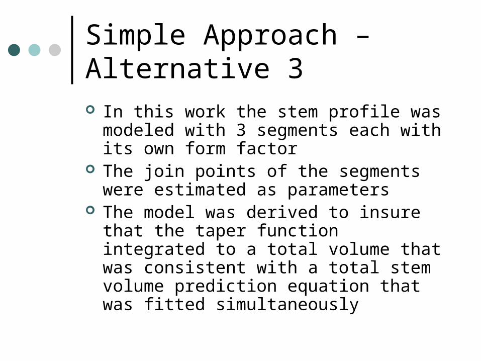
Simple Approach – Alternative 3 In this work the stem profile was modeled

with 3 segments each with its own form factor

The join points of the segments were estimated as parameters

The model was derived to insure that the taper function integrated to a total volume that was consistent with a total stem volume prediction equation that was fitted simultaneously

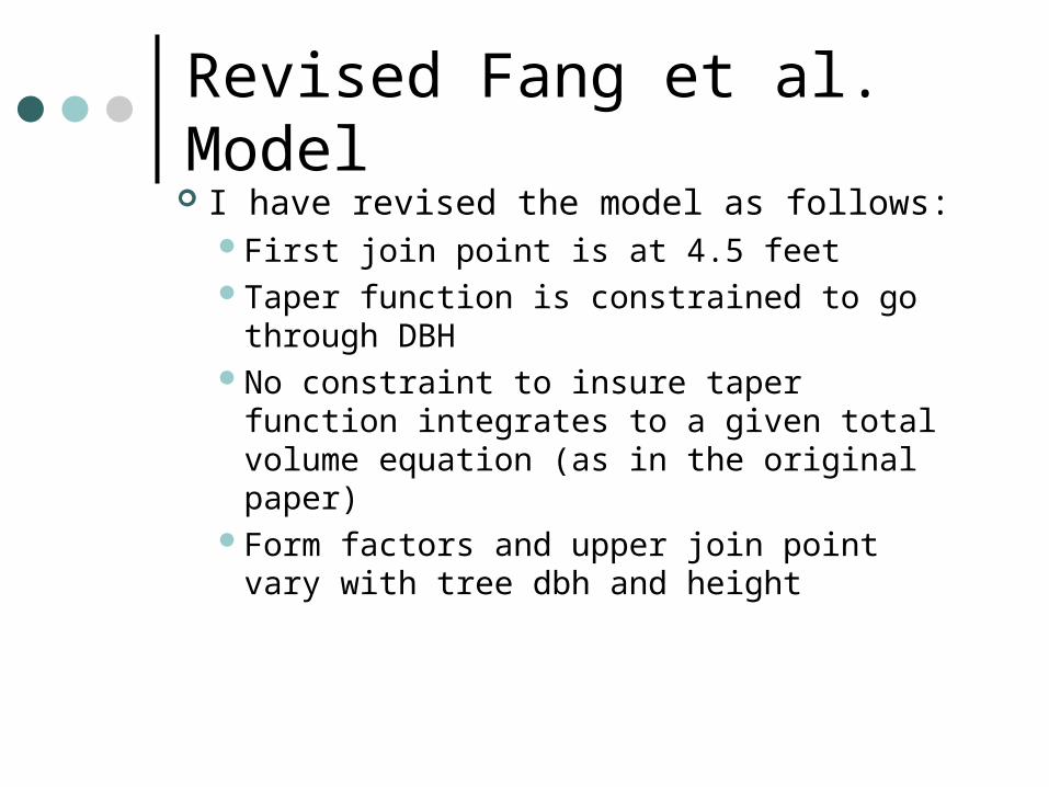
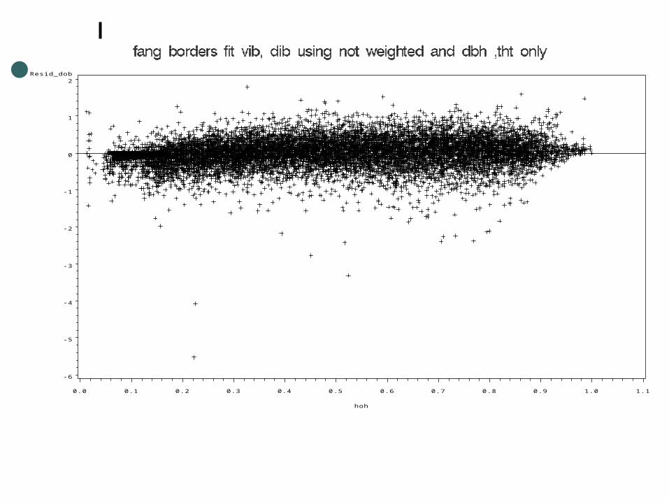
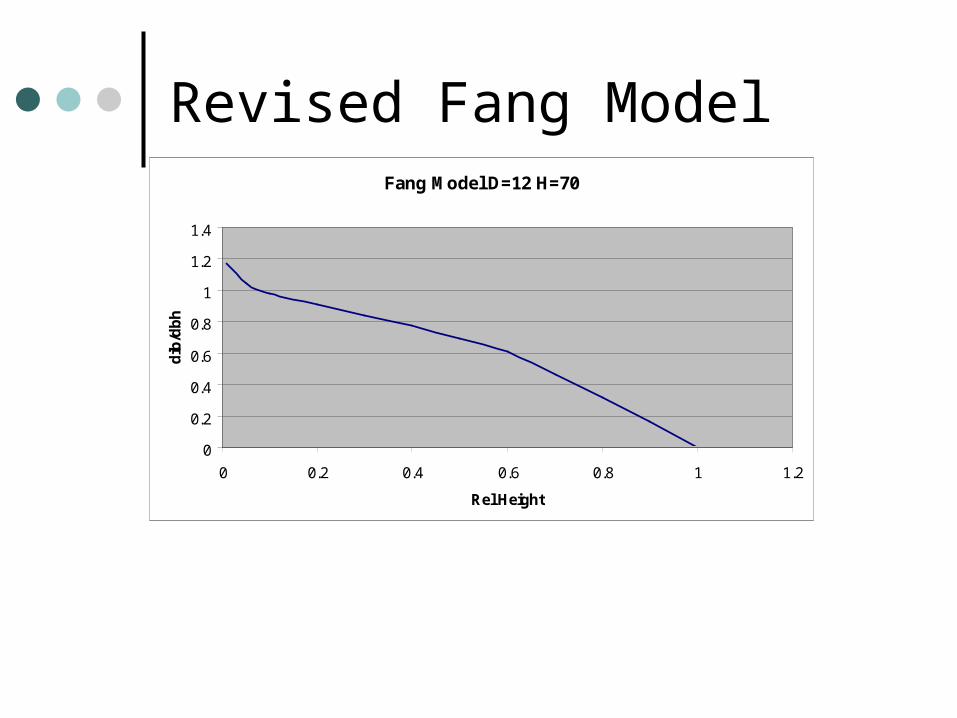
Revised Fang et al. Model I have revised the model as follows:

First join point is at 4.5 feetTaper function is constrained to go

through DBHNo constraint to insure taper function

integrates to a given total volume equation (as in the original paper)

Form factors and upper join point vary with tree dbh and height

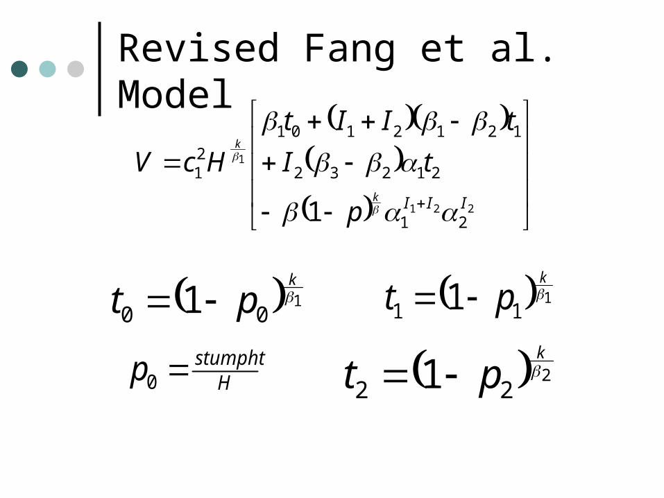
Revised Fang et al. Model2

1

2211

11

21 )1(

III

kk

pHcd

2112

11 1

k

p

3223

22 1

k

p

2121

321

1IIII

121

5.4

1

k

H

Dc 5.41 Hp 576

k Hhp

otherwise 0

1 211

pppI

otherwise 0

1 1 22

ppI

Revised Fang et al. Model

0 Hstumphtp

221

1

21

21232

1212101

21

1 IIIk

k

p

tI

tIIt

HcV

111 1

k

pt 100 1

k

pt

222 1

k

pt

oop O P

dod

0. 0

0. 1

0. 2

0. 3

0. 4

0. 5

0. 6

0. 7

0. 8

0. 9

1. 0

1. 1

1. 2

1. 3

hoh

0. 0 0. 1 0. 2 0. 3 0. 4 0. 5 0. 6 0. 7 0. 8 0. 9 1. 0 1. 1

Resi d_dob

- 5

- 4

- 3

- 2

- 1

0

1

2

3

4

hoh

0. 0 0. 1 0. 2 0. 3 0. 4 0. 5 0. 6 0. 7 0. 8 0. 9 1. 0 1. 1

Resi d_vob

- 6

- 5

- 4

- 3

- 2

- 1

0

1

2

3

4

5

6

hoh

0. 0 0. 1 0. 2 0. 3 0. 4 0. 5 0. 6 0. 7 0. 8 0. 9 1. 0 1. 1

oop O P

dod

0. 0

0. 1

0. 2

0. 3

0. 4

0. 5

0. 6

0. 7

0. 8

0. 9

1. 0

1. 1

1. 2

1. 3

hoh

0. 0 0. 1 0. 2 0. 3 0. 4 0. 5 0. 6 0. 7 0. 8 0. 9 1. 0 1. 1

Resi d_dob

- 6

- 5

- 4

- 3

- 2

- 1

0

1

2

hoh

0. 0 0. 1 0. 2 0. 3 0. 4 0. 5 0. 6 0. 7 0. 8 0. 9 1. 0 1. 1

Resi d_vob

- 6

- 5

- 4

- 3

- 2

- 1

0

1

2

3

4

5

hoh

0. 0 0. 1 0. 2 0. 3 0. 4 0. 5 0. 6 0. 7 0. 8 0. 9 1. 0 1. 1

Revised Fang ModelFang dod vs Rel Ht

0

0.2

0.4

0.6

0.8

1

1.2

0.1 0.2 0.3 0.4 0.5 0.6 0.7 0.8 0.9 1

Rel ht

do

b/d

bh

D10_H60

D12_H60

D14_H60

D16_H60

Fang dod vs Rel Ht

0

0.2

0.4

0.6

0.8

1

1.2

0.1 0.2 0.3 0.4 0.5 0.6 0.7 0.8 0.9 1

Rel Ht

do

b/d

bh

D12_H50

D12_H60

D12_H70

D12_H80

Revised Fang ModelFang Model D=12 H=70

0

0.2

0.4

0.6

0.8

1

1.2

1.4

0 0.2 0.4 0.6 0.8 1 1.2

Rel Height

dib

/db

h

Not So Simple Approach (Because Tree Shapes Are Not So Simple!!)

Clark, Souter and Schlaegel 1991 Souter and Clark 2001

Clark, A. III, R.A. Souter and B. Schlaegel. 1991. Stem profile equations for southern tree species. Research Paper SE-282. Asheville, NC. USDA Forest Service, Southeastern For Exp Sta. 113 pp.

Souter, R.A. and A. Clark III. 2001. Taper and volume prediction in southern tree species. USDA For. Serv. Southern Research Station. FIA Work Unit Administrative Report.

Souter & Clark Model

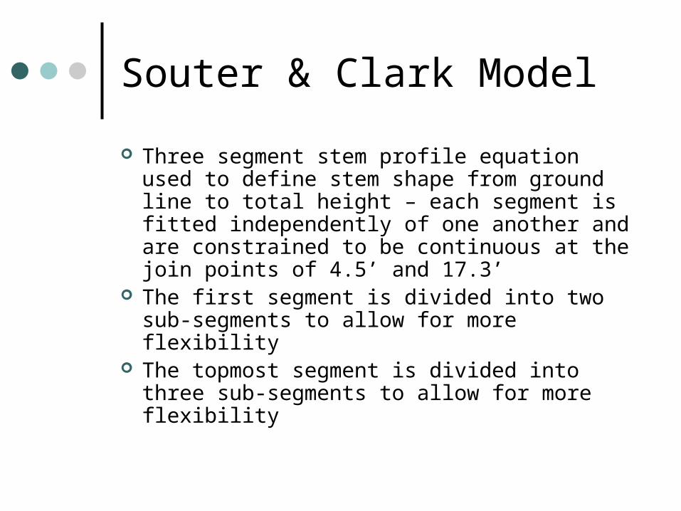
Three segment stem profile equation used to define stem shape from ground line to total height – each segment is fitted independently of one another and are constrained to be continuous at the join points of 4.5’ and 17.3’

The first segment is divided into two sub-segments to allow for more flexibility

The topmost segment is divided into three sub-segments to allow for more flexibility

Souter & Clark Model

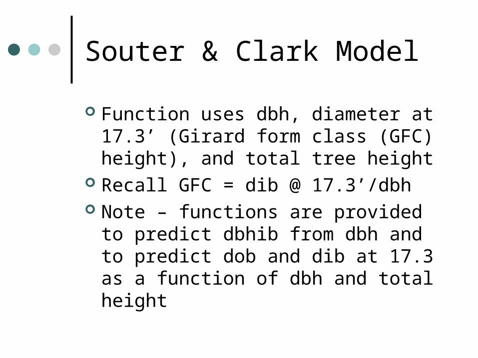
Function uses dbh, diameter at 17.3’ (Girard form class (GFC) height), and total tree height

Recall GFC = dib @ 17.3’/dbh Note – functions are provided to

predict dbhib from dbh and to predict dob and dib at 17.3 as a function of dbh and total height

Figure 3: Taper model for use at heights between ground line and 4.5'. Parameters, J, r, s, and c, are predicted as

functions of dbh (ob) and total tree height. Ground line diameter, D0, is not measured but predicted with the flare parameter, c, and the provided diameter, D4.5.

c I

+J c I D = d

h- r

J

h- ss)-(rJ2

.5

)1(

)1)(1(

5.45.4

5.45.4

5.4

D0=D4.5 (1+c)

h

4.5'

d

D4.5

0'

hJ=4.5(1-J)

h<hJ IJ =1

Figure 2: Taper model for use at heights between 4.5' and 17.3'. The parameter, p, is predicted as a function of dbh

(ob) and total tree height. The flare parameter c17 is not predicted, but is calculated using the diameters at 4.5' and 17.3' that are provided, D4.5 and D17.3, respectively.

D17.3

h

17.3'

d

D4.5=D17.3 (1+c17)

4.5'

cD = d17.3

h- p217.3

.5

5.43.17

171

D17.3

H

h

17.3'

d

h1=H-a1(H-17.3')

DH=0

h2=H-a2(H-17.3')

h<h1 Ia1 =1

h1<h<h2 Ia2 =1

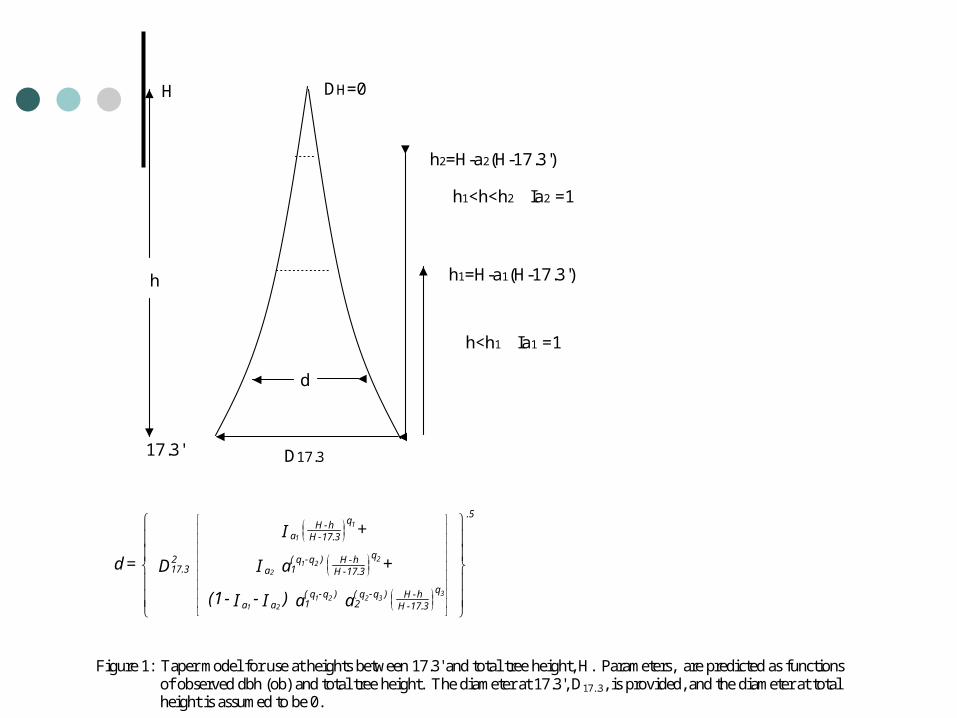
Figure 1: Taper model for use at heights between 17.3' and total tree height, H. Parameters, are predicted as functions

of observed dbh (ob) and total tree height. The diameter at 17.3', D17..3, is provided, and the diameter at total height is assumed to be 0.

a a )I-I-(1

+ a I

+ I

D = d

17.3-Hh-H q)q-q(

2)q-q(

1aa

17.3-Hh-H q)q-q(

1a

17.3-Hh-H q

a

217.3

.5

33221

21

221

2

1

1

1.

)5.40()1(

)1)(1(

)3.175.4(1

)3.17(

5.45.4

5.45.4

5.4

5.43.17

17 eq

h if c I

+J c I D

h if c D

Hh if

a a )I-I-(1

+ a I

+ I

D

= d

h- rJ

h- ss)-(rJ

2

17.3h- p2

17.3

17.3-Hh-H q)q-q(

2)q-q(

1aa

17.3-Hh-H q)q-q(

1a

17.3-Hh-H q

a

217.3

.5

33221

21

221

2

1

1

Souter & Clark Taper Function

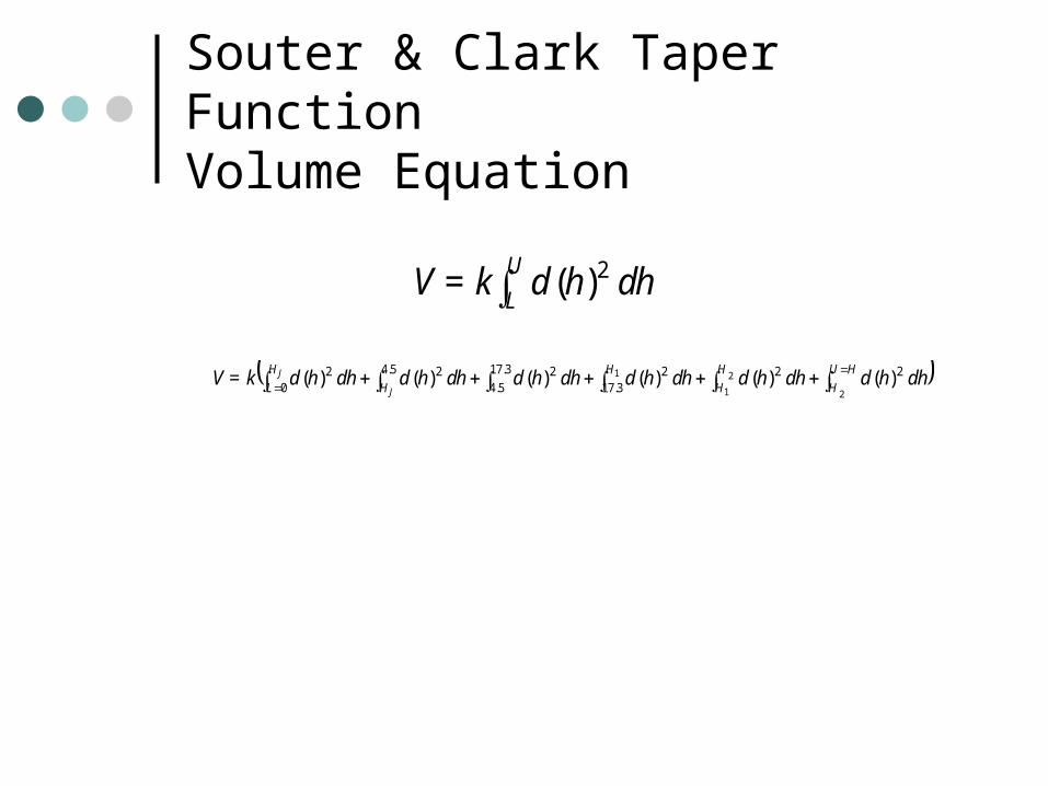
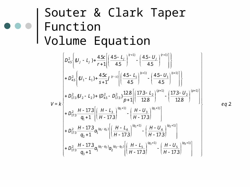
Souter & Clark Taper FunctionVolume Equation

dhhdk= VU

L2)(

dhhddhhddhhddhhddhhddhhdk= VHU

H

H

H

H

H

H

L J

J

2

2

1

1 223.17

23.17

5.425.4 2

02 )()()()()()(

Souter & Clark Taper FunctionVolume Equation

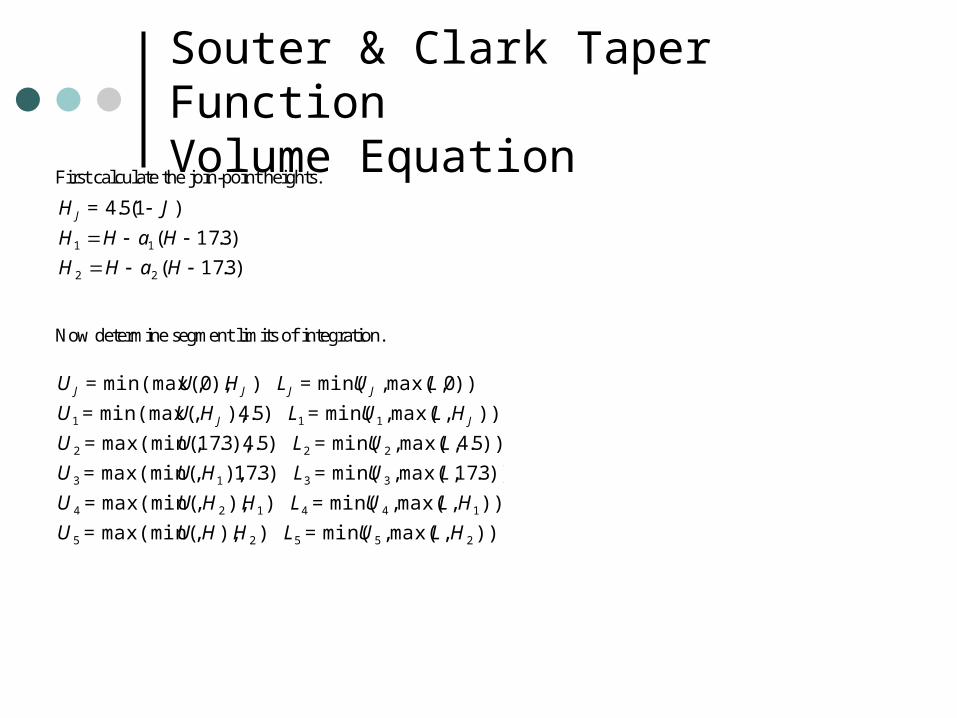
First calculate the join-point heights.

Now determine segment limits of integration.

)3.17(

)3.17(

)1(5.4

22

11

HaHH

HaHH

J= H J

)),max(,min()),,max(min(

)),max(,min()),,max(min(

))3.17,max(,min()3.17),,max(min(

))5.4,max(,min()5.4),3.17,max(min(

)),max(,min()5.4),,min(max(

))0,max(,min()),0,min(max(

25525

144124

3313

222

111

HLU= LHHU= U

HLU= LHHU= U

LU= LHU= U

LU= LU= U

HLU= LHU= U

LU= LHU= U

JJ

JJJJ

Souter & Clark Taper FunctionVolume Equation

2.

3.173.171

3.17

3.173.171

3.17

3.173.171

3.17

8.12

3.17

8.12

3.17

1

8.12)()(

5.4

5.4

5.4

5.4

1

5.4)(

5.4

5.4

5.4

5.4

1

5.4)(

)1(5

)1(5)(

2)(

13

23.17

)1(4

)1(4)(

12

23.17

)1(3

)1(3

1

23.17

)1(2

)1(22

3.172

5.4222

3.17

)1(1

)1(1)(

112

5.4

)1()1(2

5.4

33

3221

2221

11

eq

qqqqqq

qqqq

qq

pp

sssr

rJ

rJ

JJ

H

UH

H

LHaa

q

HD

H

UH

H

LHa

q

HD

H

UH

H

LH

q

HD

UL

pDDLUD

ULJ

s

cLUD

UL

r

cLUD

k= V

Souter & Clark Taper FunctionHeight Prediction for Given Top Diameter

3.eq

)1(0

)1()1(1

15.45.4

)1(1

15.45.4

8.123.17

3.17

3.17

03.17

5.42

5.42

5.4

1

25.4

2

5.42

5.4

1

)(25.4

2

3.172

5.4

1

3.175.4

3.172

13.172

3.17

1

3.17

2

213.172

13.17

1

3.17

2

1

2213.17

1

3.17

2

21

11

22112

12

2213

2312

cD d if

J cD d cD if c

D dJ cD if cJ

D dD if D D

D d

aD dD if D

dHH

aaD daD if D

daHH

daaDif D

daaHH

= h

2

r22r

D

d

2r2s

srD

d

22p

22

2

q22q

2

qqq2q2q

2

qq

qqq2q

2

qqqq

Souter & Clark Taper FunctionAuxiliary Variable Prediction

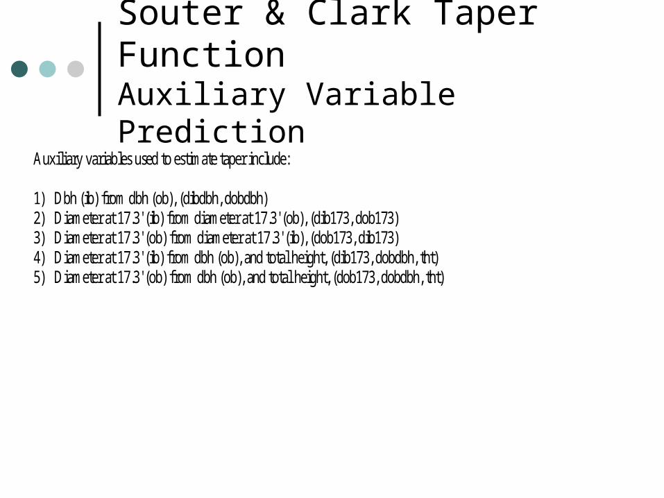
Auxiliary variables used to estimate taper include: 1) Dbh (ib) from dbh (ob), (dibdbh, dobdbh) 2) Diameter at 17.3' (ib) from diameter at 17.3' (ob), (dib173, dob173) 3) Diameter at 17.3' (ob) from diameter at 17.3' (ib), (dob173, dib173) 4) Diameter at 17.3' (ib) from dbh (ob), and total height, (dib173, dobdbh, tht) 5) Diameter at 17.3' (ob) from dbh (ob), and total height, (dob173, dobdbh, tht)

Souter & Clark Taper FunctionAuxiliary Variable Prediction

With model forms, respectively, 1) dibdbh=adibdbh+bdibdbh*dobdbh+adibdsz*dsize+bdibdsz*dsize*dobdbh; dsize is an indicator for sawtimber sizes; =1 if dbh class>=9" for softwoods, >=11" for hardwoods. Parameters are adibdbh, bdibdbh, adibdsz, and bdibdsz. 2) dib173=adibf+bdibf*dob173+adibfsz*dsize+bdibfsz*dsize*dob173; Parameters are adibf, bdibf, adibfsz, and bdibfsz. 3) dob173=adobf+bdobf*dib173+adobfsz*dsize+bdobfsz*dsize*dib173; Parameters are adobf, bdobf, adobfsz, and bdobfsz. 4) dib173=dbh/(1+exp(-(edib17th+(cdib17th+ndib17th*indicsd)*dbh +ldib17th*log(tht)**2+mdib17th*indicsh +ddib17th*log(tht)+idib17th*dbh*log(tht)))); size indicator used are indicsh=(tht<30); indicsd=(dbh<=8); Parameters are edib17th, cdib17th, ndib17th, ldib17th, mdib17th, ddib17th, and idib17th. 5) dob173=dbh/(1+exp(-(edob17th+(cdob17th+ndob17th*indicsd)*dbh +ldob17th*log(tht)**2+mdob17th*indicsh+ddob17th*log(tht)+idob17th*dbh*log(tht)))); Parameters are edob17th, cdob17th, ndob17th, ldob17th, mdob17th, ddob17th, and idob17th.

Souter & Clark Taper FunctionAuxiliary Variable Prediction

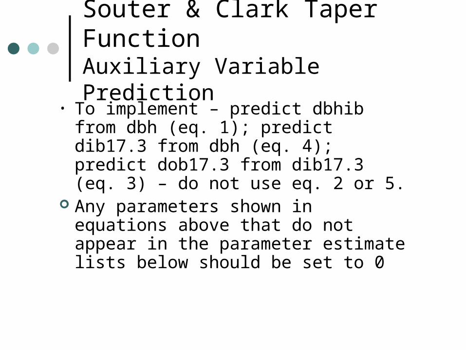
• To implement – predict dbhib from dbh (eq. 1); predict dib17.3 from dbh (eq. 4); predict dob17.3 from dib17.3 (eq. 3) – do not use eq. 2 or 5.

Any parameters shown in equations above that do not appear in the parameter estimate lists below should be set to 0

Weight Density

Clark, A. III, R.F. Daniels and B.E. Borders. 2005. Effect of rotation age and physiographic region on weight per cubic foot of planted loblolly pine. Southern Silvicultural Confernce. Memphis, TN. March 2005.

Weight Density

All individual tree weight data from the PMRC, WQC and U.S. Forest Service was used for this work

Loblolly plantations were separated into two regions – Atlantic and Gulf Coastal Plains combined and Piedmont, Upper Coastal Plain and Hilly Coastal Plain (Inland) combined

Weight Density

Weight Density

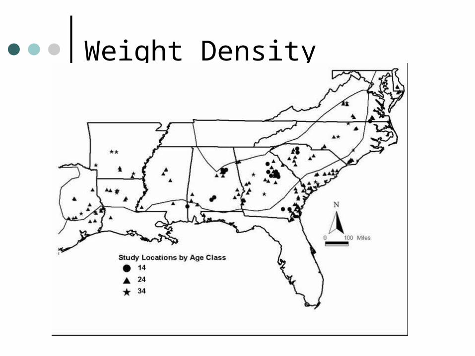
Three age classes10 to 18 years19 to 27 years> 27 years

Weight Density

Green weight of wood and bark per cubic foot of wood – can use in conjunction with inside bark cubic volume functions shown above to obtain estimated weight of wood and bark

Weight Density

Coastal Plains – 68.12 lbs wood and bark/cubic foot of wood (66.91 to 69.33)

Inland – 66.61 lbs wood and bark/cubic foot of wood (65.89 to 67.32)

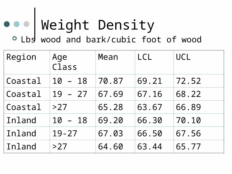
Weight Density Lbs wood and bark/cubic foot of wood

Region Age Class Mean LCL UCL

Coastal 10 – 18 70.87 69.21 72.52

Coastal 19 – 27 67.69 67.16 68.22

Coastal >27 65.28 63.67 66.89

Inland 10 – 18 69.20 66.30 70.10

Inland 19-27 67.03 66.50 67.56

Inland >27 64.60 63.44 65.77

Weight Density

Reasons why this density decreases as trees age: As dbh increases (as trees age) the

proportion of stem weight in bark decreases (thus denominator (cubic feet of wood) tends to be larger for older trees)

Wood moisture content decreases with increasing tree age (averaged 124% for 14 yr old trees, 114% for 24 yr old trees, 104% for 34 yr old trees)

Weight Density

Further work is underway to look at defining density of green weight of wood/cubic foot of wood and dry weight of wood per cubic foot of wood

Also – developing functions to predict these density measures for different tree ages along the stem and how best to use these functions in conjunction with the taper/volume functions

Summary

Bottomline – several improved functions available for taper/cubic volume/weight determination for loblolly pine plantations – user’s choice (if Clark et al. model is not used the best choice is the revised Fang model)

Same work will be done for slash pine

THE END

Remember – it is important to get out of the truck every now and then!

Revised Fang OB Fit

The MODEL Procedure Nonlinear SUR Summary of Residual Errors DF DF Adj Equation Model Error SSE MSE Root MSE R-Square R-Sq dm 4.5 14777 2489.8 0.1685 0.4105 0.9757 0.9757 vol 4.5 14777 5851.7 0.3960 0.6293 0.9886 0.9886 Nonlinear SUR Parameter Estimates Approx Approx Parameter Estimate Std Err t Value Pr > |t| pp1 -13.3103 0.4499 -29.58 <.0001 pp2 4.304361 0.1364 31.56 <.0001 pp3 -0.34946 0.0139 -25.08 <.0001 bb1 0.001325 0.000017 78.70 <.0001 bb2 -0.00004 1.955E-6 -19.26 <.0001 mm1 0.002128 0.000013 169.33 <.0001 mm2 5.103E-6 2.853E-7 17.88 <.0001 mm3 -0.00001 1.531E-6 -9.11 <.0001 bet3 0.001899 9.892E-6 191.95 <.0001

p2 = 1/(1+exp(-(pp1 + pp2*log(tht) + pp3*dbh))); bet1 = bb1 + bb2*dbh; bet2 = mm1 + mm2*tht +mm3*dbh;

Revised Fang IB Fit

The MODEL Procedure Nonlinear SUR Summary of Residual Errors DF DF Adj Equation Model Error SSE MSE Root MSE R-Square R-Sq dm 4.5 14777 2172.6 0.1470 0.3834 0.9737 0.9737 vol 4.5 14777 5062.0 0.3426 0.5853 0.9868 0.9868 Nonlinear SUR Parameter Estimates Approx Approx Parameter Estimate Std Err t Value Pr > |t| pp1 -8.22247 0.2223 -36.99 <.0001 pp2 2.602632 0.0647 40.23 <.0001 pp3 -0.22236 0.00720 -30.90 <.0001 bb1 0.001468 0.000018 79.73 <.0001 bb2 -0.00006 2.293E-6 -24.25 <.0001 mm1 0.002367 0.000017 137.41 <.0001 mm2 6.763E-6 3.767E-7 17.95 <.0001 mm3 -0.00003 2.146E-6 -12.60 <.0001 bet3 0.001869 7.901E-6 236.53 <.0001

p2 = 1/(1+exp(-(pp1 + pp2*log(tht) + pp3*dbh))); bet1 = bb1 + bb2*dbh; bet2 = mm1 + mm2*tht +mm3*dbh;

Clark & Souter Taper FunctionTaper Parameters

Each parameter is predicted with unique sets of coefficients, ( , , ), with some of the estimated coefficients being 0. Parameters and model forms associated with Figure 1: q1=(aq1+bq1*(tht)+cq1*dbh); a1=1/(1+exp(-(aa1+ba1*log(tht)+ca1*dbh))); q2=(aq2.+bq2*(tht)+cq2*dbh); a2=(1/(1+exp(-(aa2+ba2*log(tht)+ca2*dbh))))*a1; q3=(aq3+bq3*(tht)+cq3*dbh); Parameters and model form associated with Figure 2: p=exp(ap+bp*(tht)+cp*dbh); Parameters and model forms associated with Figure 3: J=1/(1+exp(-(aJ+bJ*log(tht)+cJ*dbh))); s.=(as+bs*(tht)+cs*dbh); r=(ar+br*(tht)+cr*dbh); c=(ac+bc*log(tht)+cc*dbh); While the above systems of taper parameters are described for outside bark diameter measurements, completely analogous parameters are used for inside bark diameter predictions, where dbh in the equations would refer to an inside bark dbh. Parameters would be subscripted with "o" or "i" to indicate the appropriate system.

NOTE – any parameters that do not appear in the estimate lists below should be set to 0.

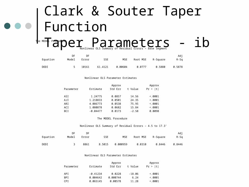
Clark & Souter Taper FunctionTaper Parameters - ib

The MODEL Procedure Nonlinear OLS Summary of Residual Errors – Base Segment DF DF Adj Equation Model Error SSE MSE Root MSE R-Square R-Sq DODI 5 10161 61.4121 0.00604 0.0777 0.5880 0.5878 Nonlinear OLS Parameter Estimates Approx Approx Parameter Estimate Std Err t Value Pr > |t| ASI 1.24775 0.0857 14.56 <.0001 AJI 1.218833 0.0501 24.35 <.0001 ARI 4.086773 0.0538 75.95 <.0001 ACI 1.080878 0.0682 15.84 <.0001 BCI -0.04477 0.0173 -2.58 0.0098 The MODEL Procedure Nonlinear OLS Summary of Residual Errors – 4.5 to 17.3’ DF DF Adj Equation Model Error SSE MSE Root MSE R-Square R-Sq DODI 3 8861 8.5015 0.000959 0.0310 0.8446 0.8446 Nonlinear OLS Parameter Estimates Approx Approx Parameter Estimate Std Err t Value Pr > |t| API -0.41234 0.0228 -18.06 <.0001 BPI 0.004642 0.000744 6.24 <.0001 CPI 0.065145 0.00578 11.28 <.0001

Clark & Souter Taper FunctionTaper Parameters - ib

The MODEL Procedure – 17.3’ to Tip Nonlinear OLS Summary of Residual Errors DF DF Adj Equation Model Error SSE MSE Root MSE R-Square R-Sq DODI 12 18978 29.8629 0.00157 0.0397 0.9619 0.9619 Nonlinear OLS Parameter Estimates Approx Approx Parameter Estimate Std Err t Value Pr > |t| AQ1I 1.111066 0.0225 49.46 <.0001 CQ1I -0.01107 0.00250 -4.43 <.0001 AQ2I 2.480819 0.0374 66.40 <.0001 BQ2I -0.04164 0.00116 -35.96 <.0001 CQ2I 0.162101 0.00642 25.24 <.0001 AQ3I 1.884622 0.0534 35.29 <.0001 BQ3I -0.01296 0.00110 -11.80 <.0001 CQ3I 0.080945 0.00509 15.91 <.0001 AA1I 12.55434 0.3893 32.25 <.0001 BA1I -2.85796 0.0947 -30.19 <.0001 AA2I -12.0778 0.9261 -13.04 <.0001 BA2I 3.192642 0.2285 13.97 <.0001

Souter & Clark Taper FunctionPredict dbhib from dbhThe GLM Procedure

Dependent Variable: DIBDBH Sum of Source DF Squares Mean Square F Value Pr > F Model 1 8736.638139 8736.638139 95266.6 <.0001 Error 2644 242.473898 0.091707 Corrected Total 2645 8979.112037 R-Square Coeff Var Root MSE DIBDBH Mean 0.972996 4.554590 0.302832 6.648942 Source DF Type I SS Mean Square F Value Pr > F DOBDBH 1 8736.638139 8736.638139 95266.6 <.0001 Source DF Type III SS Mean Square F Value Pr > F DOBDBH 1 8736.638139 8736.638139 95266.6 <.0001 Standard Parameter Estimate Error t Value Pr > |t| Intercept -.4344503820 0.02369246 -18.34 <.0001 DOBDBH 0.9180106242 0.00297425 308.65 <.0001

Souter & Clark Taper FunctionPredict dib173 from dbh

The MODEL Procedure Nonlinear OLS Summary of Residual Errors DF DF Adj Equation Model Error SSE MSE Root MSE R-Square R-Sq DIB173 7 2684 360.3 0.1342 0.3664 0.9612 0.9611 Nonlinear OLS Parameter Estimates Approx Approx Parameter Estimate Std Err t Value Pr > |t| cdib17th -0.32344 0.0641 -5.04 <.0001 ddib17th 8.990871 0.8436 10.66 <.0001 edib17th -18.01 1.4740 -12.22 <.0001 idib17th 0.075332 0.0157 4.79 <.0001 ldib17th -1.04591 0.1195 -8.75 <.0001 mdib17th -0.10512 0.0421 -2.50 0.0127 ndib17th -0.00662 0.00205 -3.23 0.0013

Souter & Clark Taper FunctionPredict dob173 from dib173

The MODEL Procedure Nonlinear OLS Summary of Residual Errors DF DF Adj Equation Model Error SSE MSE Root MSE R-Square R-Sq DOB173 4 2687 105.5 0.0393 0.1981 0.9900 0.9900 Nonlinear OLS Parameter Estimates Approx Approx Parameter Estimate Std Err t Value Pr > |t| adobf 0.223475 0.0200 11.15 <.0001 bdobf 1.048978 0.00434 241.70 <.0001 adobfsz 0.183364 0.0472 3.88 0.0001 bdobfsz -0.01595 0.00698 -2.28 0.0225