Individual Taxes and the Distribution of Income 3 Individual Taxes and the Distribution of Income...

This PDF is a selection from an out-of-print volume from the NationalBureau of Economic Research

Volume Title: The Personal Distribution of Income and Wealth

Volume Author/Editor: James D. Smith, ed.

Volume Publisher: NBER

Volume ISBN: 0-870-14268-2

Volume URL: http://www.nber.org/books/smit75-1

Publication Date: 1975

Chapter Title: Individual Taxes and the Distribution of Income

Chapter Author: Benjamin A. Okner

Chapter URL: http://www.nber.org/chapters/c3751

Chapter pages in book: (p. 45 - 74)

CHAPTER 3

Individual Taxes and theDistribution of Income

Benjamin A. OknerThe Brookings Institution

Most economists agree that the most appropriate way tomeasure the burden or incidence of taxes is in terms of their effecton the distribution of income. There is so little dispute, in fact,that incidence is usually defined simply as the effect of taxes onthe distribution of income available for private use.

In order to determine empirically the burden of any tax, someassumption must be made about whose real income it reduces andabout the amount of before-tax income that would have beenreceived in its absence. Since taxes affect the total level ofeconomic output as well as the distribution of real income throughtheir impact on both factor prices (the sources of income) andcommodity prices (the uses of income), a full-fledged study of theoverall burden of taxes is exceedingly complex.

In this paper, I am concerned only with the distributionaleffects of the personal income and employment taxes. Since thesetwo levies amounted to more than 50 percent of total governmenttax receipts in 1966,1 their incidence is of considerable impor-tance for any overall study of tax burdens. In addition, there is

The views presented are those of the author and not necessarily those ofthe officers, trustees, or other staff members of The Brookings Institution.All computer operations described in the paper were performed at theBrookings Social Science Computation Center and the programming was doneby Andrew D. Pike, whose efforts are gratefully acknowledged. The workdescribed is part of a research program supported by a grant from the U.S.Office of Economic Opportunity.

1 Total government tax receipts in the study are equal to federal, state,and local government receipts as measured in the National Income Accounts,adjusted to exclude nontaxes, intergovernmental grants-in-aid, and socialinsurance contributions for civilian government retirement funds and vet-erans' life insurance.

45

46 Benjamin A. Okner

little disagreement as to how these taxes should be allocatedamong persons.2

Once one has decided how a given tax should be allocatedamong individuals in the population, its incidence—or impact onthe distribution of income—might be presumed to be a ratherstraightforward calculation. However, this is not necessarily thecase, because there are a number of ways in which income mightbe defined. Although we prefer a particular income definition, atthe beginning of the analysis some attention is given to alternativeincome concepts which might be used in an incidence study.

In addition to the overall distributions of before- and after-taxincome, we also examine and compare the incidence of individualtaxes for specific subgroups of the population. And since weinterpret individual taxes broadly to include transfer paymentsreceived from the government as well as taxes paid, we assess theextent to which both individual taxes and transfers affect thedistribution of income in our analysis.

METHODOLOGY AND DATA

The results presented are all based on the Brookings MERGEFile which contains demographic and financial data for a sample•of 72,000 families and single individuals in calendar year 1966.This file was created by combining information from the 1967Survey of Economic Opportunity (SEO) and data from the 1966Tax File, which contains income and tax information from federalindividual income tax returns filed for 1966. The basic unit ofanalysis in the MERGE File is the Census family or unrelatedindividual.

2 While it is possible that individuals might change their allocation of timebetween work and leisure because of the individual income tax, there are feweconomists who believe that this would be a significant factor. Therefore, wefollow the traditional practice of allocating personal income taxes directlyamong individuals on the basis of their incomes under the assumption that weneed not take account of tax-induced changes in the distribution ofbefore-tax income. In the case of employment taxes, even though there is notunanimous agreement as to the incidence of such levies, we follow theprevalent modern practice of allocating both the employer and employeeshares of these taxes among persons on the basis of their compensation fromearnings. For a detailed discussion of the reasoning and various views on thissubject, see John A. Brittain, The Payroll Tax for Social Security (Wash-ington, D.C.: Brookings Institution, 1972).

A detailed description of the MERGE File and how it was created isgiven in Benjamin A. Okner, "Constructing a New Data Base from Existing

Individual Taxes and Distribution of Income 47

Since all the calculations are based on microunit data in theMERGE File, the methodology used here differs considerablyfrom previous empirical tax burden studies. In the past, individualtaxes were allocated to broad income classes on the basis of a largenumber of statistical series which were used as proxies for the taxdistributions.4 The major disadvantage of such methodology isthat it requires that taxes be distributed on the basis of the averageincome and behavior of all households in a particular income class,rather than on the basis of the income and behavior of theindividual microunits in the class.

Although we could not make all the distinctions that arerelevant for estimating tax liabilities, the MERGE File provides uswith a very rich source of information for this purpose. Amongthe characteristics that are particularly important for estimatingtax payments are sources of income, marital status and familycomposition, consumption patterns, and home ownership. Sincethis information is available for each unit in the file, whenever it isnecessary to make assumptions about the economic behavior ofhouseholds, we are not limited to a single assumption for allfamilies in a given income class. This frees us from the uniformityassumption which has been the hallmark of all past studies.

In addition to this major improvement in methodology, theMERGE File permits us to prepare tax burden distributions on thebasis of various alternative incidence assumptions and incomedefinitions. In the past, these were impossible because of the sheermagnitude of the computational job. As illustrated below, the newfile, along with present electronic computer capabilities, gives usgreat flexibility in this respect.

BEFORE-TAX DISTRIBUTION OF INCOME

There is no single concept of income that is acceptable anduseful for all analytical purposes. However, for analyzing theincidence of taxes it is clearly inappropriate to compare taxpayments with income subject to tax; we are interested in acomparison between taxes paid and total incomes. To provide thistype of information, we adopted a comprehensive income defini-

Microdata Sets: The 1966 MERGE File," Annals of Economic and SocialMeasurement 1 (July 1 972):325-42.

The classic study along these lines is by Richard A. Musgrave and others,"Distribution of Tax Payments by Income Groups: A case Study for 1948,"National Tax Journal 4 (March 195 1):11-54.

48 BenjaminA. Okner

tion that is intended to correspond as closely as is practical to aneconomic concept of income, viz., consumption plus tax paymentsplus (or minus) the net increase (or decrease) in the value of assetsduring the year. This concept, called family income (Fl), is thesum of national income (as defined in the National IncomeAccountS)5 plus transfer payments plus accrued gains on farmassets and nonfarm real estate6 In keeping with the nationalincome concept, Fl includes corporation income before tax. Thisprocedure has the advantage not only of consistency but also ofproviding a complete account of the accrued income claims of thehousehold sector. Retained earnings of corporations, which areincluded in family income, may be regarded as an approximationof accrued capital gains on corporate stock during the year.7 Flincludes only income which accrues directly to families andindividuals, and thus excludes the income received by fiduciariesand persons in the institutional population not represented in theSEO File.

Other income concepts that might be employed are moneyfactor income, Census money income, and total money receipts.The relationship among these four concepts is illustrated in Table1. Money factor income includes the $484 billion moneyincome received by individuals from production. To this we addwage supplements, net imputed rent, accrued capital gains on farmassets and nonfarm real estate, corporate retained earnings and the

The major departure from the official definition of income is theomission of interest imputed to individuals for the services rendered to themby the banking system.

6 For a detailed description, see Benjamin A. Okner, "Adjusted FamilyIncome: Concept and Derivation," Brookings Technical Working Paper II, forthe Distribution of Federal, State and Local Taxes Research Program, rev.,processed (Washington, D.C.: Brookings Institution, August 1972), which isavailable on request.

We used this approximation because the annual fluctuations in the valueof corporate stock are very large and even three- to five-year averages may notgive an adequate representation of accrued capital gains. Martin J. Bailey andMartin David have shown that over very long periods of time, capital gains oncorporate securities are roughly equal to retained earnings. See Martin J.Bailey, "Capital Gains and Income Taxation," in Arnold C. Harberger andMartin J. Bailey, eds., The Taxation of Income from Capital (Washington,D.C.: Brookings Institution, 1969), pp. 15-26; and Martin David,AlternativeApproaches to Capital Gains Taxation (Washington, D.C.: Brookings Institu-tion, 1968), pp. 242-46.

Individual Taxes and. Distribution of Income 49

TABLE I Comparison of Various Income Concepts, 1966

(billions of dollars)

Item Amount

Money factor incomea 484

Plus: Wage supplementsb 41

Net imputed rent 11

Retained corporate profits 22Corporation income tax 26Accrued gains on farm assets and nonfarm real estate 37Interest on life insurance policies 6

Subtotal 142

Equals family income before transfers 627

Less total nonmoney income —142

Plus: Private pensions 6

Civilian and military government pensions 6Other income 7

Subtotal —124

Equals Census money income before transfers 503Plus realized gains on asset sales 19

Equals total money receipts before transfers 523

Memorandum: transfer 34

a Money factor income is the sum of wages and salaries, interest, dividends, rents androyalties, and farm and nonfarm proprietors' income.

b Wage supplements mclude employer contributions to private pension and welfarefunds, Social Security, workmen's compensation, unemployment insurance, and civiliangovernment retirement systems.

C Transfer payments include Social Security benefits, public assistance, veterans'disability compensation and pensions; workmen's compensation, and unemploymentinsurance payments received by individuals.

corporation income tax allocated to individual stockholders,8 andinterest on life insurance policies to obtain total Fl beforetransfers of $624 billion. Since the Census income concept doesnot include nonmoney items, it is necessary to subtract the $141billion of such income from Fl before transfers and then addreceipts from private pensions and civilian government and

8 This excludes the portion of the tax attributable to fiduciaries andorganizations not represented in the SEO universe.


military retirement pay to derive the $502 billion of Censusmoney income before transfers.9 Finally, because the Bureau ofthe Census does not include profits from the sale of assets in itsincome concept, we add $19 billion of realized capital gains toderive $521 billion of total money receipts before transfers.

These four different concepts vary considerably in theircoverage. Family income is the most comprehensive concept,while money factor income is least inclusive. And as might beexpected, the before tax and transfer distribution of income isquite different, depending on which concept is used. InTable 2 we present the distribution of income by size class undereach of the four different definitions. (In Table 2, the incomeclasses are defined in terms of each of the specific incomedefinitions; therefore, the same family units are not included inthe same income class under the various definitions.)

In Table 3, we show the same distributions by populationquintiles under the different income definitions. Based on the datain Table 3, it is obvious that one can reach very differentconclusions about the distribution of income depending uponwhat income concept is used. For example, under the Flconcept, the lowest quintile includes families with incomes under$2,799; under the least comprehensive money factor income(MFI) concept, the lowest quintile includes those with incomes ofless than $2,368, At the other end of the income distribution, thetop quintile under the Fl concept is comprised of families withincomes of $14,564 and over, whereas under the MFI definition,the highest quintile starts at $12,446. The absolute differences inincome increase even more at the very highest levels; the top onepercent of units are those with $44,318 of MFI while the toppercentile under the Fl concept begins at $50,000.

As measured by the Gini coefficient,1° the distributions also

Under our definition, only social insurance benefits financed by payrolltaxes are treated as transfer payments. Benefits paid under governmentretirement programs are treated like private pensions and annuities and,therefore, are excluded from transfers. Government contributions, if any, tothese programs are considered income during the current year and benefitpayments received are viewed as representing only a change in the form ofasset holding by individuals (i.e., cash is increased and a prepaid insuranceasset is reduced).

1 ° The Gini coefficient of inequality is a statistical measure of overallequality or inequality in the distribution of income. Pictorially, it is equal tothe ratio of the area between the Lorenz curve and the line of equaldistribution to the entire area below the line of equal distribution. The value


TABLE 2 Distribution of Income Before Taxes and Transfers UnderVarious Income Definitions, by Income Class, 1966

(millions of dollars and percent)

Income Money Census TotalClassesa Factor Family Money Money($000) Income Income Income Receipts

Under 3b 10,724 10,784 11,386 11,2863- 5 28,053 23,563 29,578 29,4505- 10 151,516 133,594 152,566 151,284

10- 15 138,406 162,444 139,953 139,28615- 20 61,959 101,637 68,538 69,924

20- 25 24,304 50,054 26,679 28,017

25- 50 43,712 72,894 46,784 51,78250- 100 15,937 28,881 16,665 20,112

100- 500 8,153 29,470 8,643 14,224

500-1,000 655 4,854 681 2,0511,000 and over 632 6,658 645 3,178

All classes 484,050 624,833 502,118 520,594

Percentage Distributions

Under3b 2.2 1.7 2.3 2.23- 5 5.8 3.8 5.9 5.75- 10 31.3 21.4 30.4 29.1

10- 15 28.6 26.0 27:9 26:815- 20 12.8 16.3 13.6 13.4

20- 25 5.0 8.0 5.3 5.425- 50 9.0 11.7 9.3 9.950- 100 3.3 4.6 3.3 3.9

100- 500 1.7 4.7 1.7 2.7500-1,000 0.1 0.8 0.1 0.4

1,000 and over 0.1 1.1 0.1 0.6

All classes 100.0 100.0 100.0 100.0

NOTE: Details may not add to totals because of rounding.a The income class is defined in terms of the income distribution for each of the

concepts.Includes negative incomes.

of the Gini coefficient varies between 0 (indicating perfect equality) and I(indicating perfect inequality). A decrease in the value of the coefficientsignifies a more equal distribution; an increase signifies a more unequaldistribution.

Mon

ey F

acto

r In

com

eFa

mily

Inc

ome

Cen

sus

Mon

eyIn

com

eT

otal

Mon

ey R

ecei

pts

Perc

ent

Perc

ent

Perc

ent

Perc

ent

ofof

ofof

Popu

latio

nIn

com

eIn

com

eIn

com

eIn

com

eIn

com

eIn

com

eIn

com

eIn

com

eQ

uint

ileR

ange

Rec

eive

dR

ange

Rec

eive

dR

ange

Rec

eive

dR

ange

Rec

eive

d

Low

est 5

thU

nder

$2,

368

1.41

Und

er $

2,79

91.

90U

nder

$2,

482

2.05

Und

er $

2,50

22.

01Se

cond

5th

2,36

8- 5

,389

9.50

2,79

9- 6

,534

9.30

2,48

2- 5

,582

9.79

2,50

2-5,

630

9.54

Mid

dle

5th

5,38

9- 8

,383

17.0

76,

534-

9,9

8216

.07

5,58

2- 8

,567

17.0

05,

630-

8,63

416

.53

Four

th 5

th8,

3834

2,44

624

.57

9,98

2-14

,564

23.2

98,

567-

12,7

3624

.22

8,63

4-12

,884

23.7

2H

ighe

st 5

th12

,446

and

ove

r47

.39

14,5

64 a

nd o

ver

49.4

412

,736

and

ove

r46

.94

12,8

84 a

nd o

ver

48.3

0T

op 5

per

cent

19,5

76 a

nd o

ver

20.2

324

,459

and

ove

r23

.48

19,8

48 a

nd o

ver

20.0

520

,714

and

ove

r21

.80

Top

1 p

erce

nt44

,318

and

ove

r7.

5650

,000

and

ove

r11

.02

44,5

65 a

nd o

ver

7.42

46,1

52 a

nd o

ver

9.01

Gin

i coe

ffic

ient

of

ineq

ualit

ya.4

601

.474

6.4

489

.462

2

a T

he G

ini c

oeff

icie

nt o

f in

equa

lity

is a

sta

tistic

al m

easu

re o

f ov

eral

l equ

ality

in th

e di

stri

butio

n of

inco

me.

It m

ay v

ary

betw

een

0(i

ndic

atin

g pe

rfec

t equ

ality

) an

d 1

(ind

icat

ing

perf

ect i

nequ

ality

). A

dec

reas

e in

the

valu

e th

eref

ore

sign

ifie

s a

mor

e eq

ual a

lter-

tax

dist

ribu

tion

of in

com

ean

d a

mor

e pr

ogre

ssiv

e ta

x st

ruct

ure.

TA

BL

E 3

Shar

es o

f In

com

e B

efor

e T

axes

Def

initi

ons,

196

6an

d T

rans

fers

Rec

eive

d by

Eac

h Fi

fth

of th

e Po

pula

tion

Und

er V

ario

us I

ncom

e


differ substantially in the degree of inequality exhibited under thevarious income definitions. Census money income is distributedamong families most nearly equal (Cmi coefficient = .4489). Inorder of decreasing equality (increasing inequality), this isfollowed by money factor income (Gini coefficient = .460 1); totalmoney receipts (Gini coefficient = .4622); and finally, familyincome (Gini coefficient = .4746). All of the preceding coeffi-cients refer to the distributions of income exclusive of transferpayments.

DISTRIBUTION OF INDIVIDUAL TAXES AND TRANSFERS

As has been indicated, the analysis is confined to the effects ofpersonal income and employment taxes on the distribution ofindividual income. Since in this paper, we are dealing only withindividual taxes, the amount of the corporation income taxallocated to each family is excluded from family income in all theeffective tax-rate tables. However, in each table, families areclassified by the amount of total income before taxes andtransfers, i.e., total Fl less transfer payments.

The income taxes include federal and state and local taxes.Payroll taxes include employee and employer Social Securitycontributions plus employer contributions for unemploymentinsurance and workmen's compensation. Other employer socialinsurance contributions—such as those for pension and healthfunds—are not considered taxes and are excluded from theanalysis. Transfer payments include all benefits paid to individualsunder government programs, regardless of whether they arefinanced by general revenue or by payroll taxes.'1

Personal Income Taxes

The MERGE File contains the federal individual income taxreported by each taxpaying unit in 1966, so there is no need toallocate these taxes among families in the file.

State and local income taxes reported as itemized deductions ontax returns amounted to approximately 70 percent of the totalcollections reported for 1966. However, for units that did not

1 1 Business transfer payments, as defined in the National IncomeAccounts, are not included in our transfer payment (or income) definition.


itemize their deductions, we estimated the state and local incometax liability on the basis of income. family size, and place ofresidence. 12

Total personal income tax collections (less refunds) in theNational Income Accounts were $64.0 billion in 1966; this wascomprised of $58.6 billion in federal collections and $5.4 billionin state and local government collections. The $55.4 billion offederal tax collections in the MERGE File amounts to about 90percent of the national income amount. We did not attempt toadjust the MERGE figures to the national income total andaccepted the amount reported.'3 State and local income taxesallocated to MERGE File units were $5.4 billion. The totalamount of personal income taxes allocated among families in thefile is therefore $60.8 billion.

Total federal income taxes amount to 9.2 percent of income,while total state and local income taxes equal 0.9 percent of Fl.These taxes as a percentage of total Fl in each income class areshown in Table 4•14 As can be seen, both federal and state andlocal income taxes are progressive throughout most of the incomedistribution. However, for most families, total personal income taxrates are quite low. The federal income tax never exceeds 20.7percent of total income, and the highest effective rate of state andlocal income taxes is only 1 .9 percent. The effective tax rate is 10percent or less for all families with incomes below $20,000 andexceeds 20 percent only for those with incomes of $100,000 andabove. The highest effective rate of tax—22.7 percent—is reachedin the $500,000 to $1 million Fl class; beyond this income level,the effective income tax rate declines, because nontaxable incomeis highly concentrated among those with incomes at the very topof the income distribution.

1 2 The last criterion is needed because not all states have an individualincome tax. While it is used extensively, in 1966 there were still seventeenstates that did not levy a personal income tax.

1 3 An unknown, but probably small, part of the difference can beattributed to the fact that the SEO population differs from the nationalincome covereage.

1 Similar tables, with effective income tax rates based on the otherincome concepts, are presented in Appendix Tables A.! to A.3. In order toaid the reader, families are classified by family income less transfers in all, theAppendix Tables so that the effects of the income definition changes for thesame families may be followed.


TABLE '4 Effective Rates of Federal and State and Local IndividualIncome Taxes,a by Family Income Classes, 1966

(percent)

Family Federal State and Local TotalIncome Before Individual Individual Individual

Transfers In come Income Income($000) Tax Taxes Taxes

0- 3b 2.7 0.2 3.03- 5 4.6 0.4 5.05- 10 6.7 0.6 7.2

10- 15 8.1 0.8 8.915- 20 9.1 0.9 10.020- 25 9.9 1.1 11.025- 50 11.4 1.2 12.650- 100 17.3 1.7 19.0

100- 500 19.6 1.9 21.5500-1,000 20.7 1.9 22.7

1,000 and over 19.0 1.8 20.8

All classes 9.2 0.9 10.2

NOTE: Details may not add to totals because of rounding.a Effective tax rates are calculated on the basis of family income before transfers,

excluding the amount of corporation income tax allocated to families in the MERGEFile.

b Excludes families with negative incomes.

It is well known that average effective rates, such as thoseshown in Table 4, often obscure large variations in taxes paid bydifferent kinds of families within the same income class. Thedifferences between those who derive their incomes primarilyfrom wages and those who are primarily recipients of propertyincome were reported in a recent paper by Joseph A. Pechman.'5There are a very large number of other population subgroups thatmight be examined: two of these which are of particular interestare families of different size and those headed by aged andnonaged persons. The effective income tax rates for thesesubgroups are shown in Table 5.

1 See Joseph A. Pechman, "Distribution of Federal and State IncomeTaxes by Income Classes," Papers and Proceedings of the Thirtieth AnnualMeeting of the American Finance Association, Journal of Finance 27, no. 2(May 1972):179-91. Brookings Reprint 234.

TA

BL

E 5

Effe

ctiy

eR

ates

of

Indi

vidu

al in

com

e T

axes

a by

Age

of

Fam

ily H

ead

and

Size

of

Fam

ily, b

y Fa

mily

inco

me

Cla

sses

, 196

6(p

erce

nt)

Fam

ilyIn

com

eB

efor

eT

rans

fers

($00

0)

All

Fam

ilies

Non

aged

Fam

ilies

bA

ged

Fam

ilies

b

All

Size

s1

2

Fam

ily S

ize

All

5#Si

zes

Fam

ily S

ize

All

5+Si

zes

Fam

ily S

ize

34

12

34

12

34

5+

3C3.

04.

12.

52.

0L

8L

i3.

95.

53.

72.

31.

91.

91.

72.

01.

70.

71.

1d

3-5

5.0

8.5

4.3

4.2

2.9

L6

5.6

10.0

5.4

4.4

2.7

1.5

3.1

3.8

2.7

2.8

4.8

2.2

5-10

7.2

11.5

8.2

7.4

6.1

3.9

7.4

12.4

8.9

7.5

6.1

3.9

5.5

4.9

5.7

6.0

5.4

4.5

10-

158.

913

.810

.69.

78.

26.

79.

015

.110

.99.

78.

26.

78.

27.

48.

38.

88.

76.

115

-20

10.0

12.6

11.4

10.4

9.8

8.6

10.1

14.2

12.0

10.7

9.8

8.6

8.3

8.2

7.8

8.6

9.8

8.5

20-

2511

.012

.712

.711

.110

.89.

911

.316

.813

.511

.610

.99.

97.

65.

07.

76.

99.

210

.525

-50

12.6

11.4

12.5

13.4

12.8

12.5

13.1

16.1

13.8

13.7

12.8

12.5

8.0

6.1

7.2

10.3

12.6

6.0

50-

100

19.0

21.7

17.1

18.9

20.2

20.0

20.2

23.3

20.7

19.0

20.3

20.0

4.6

9.6

4.3

d—

100-

500

21.5

16.4

22.0

24.7

24.1

20.3

21.6

16.4

22.1

24.7

24.1

20.3

10.3

—10

.4—

——

500-

1,00

022

.719

.423

.123

.725

.923

.022

.723

.123

.725

.923

.0—

——

——

—

1,00

0an

d ov

er20

.819

.820

.323

.821

.021

.720

.819

.820

.323

.821

.021

.7—

——

——

All

clas

ses

10.2

11.6

11.3

10.5

9.8

8.7

10.5

13.3

12.5

10.7

9.8

8.7

6.2

5.0

5.8

7.7

8.5

6.6

a E

ffec

tive

tax

rate

s ar

e ca

lcul

ated

on

the

basi

s of

fam

ily in

com

e be

fore

tran

sfer

s, e

xclu

ding

the

amou

nt o

f co

rpor

atio

n in

com

e ta

x al

loca

ted

tofa

mili

es in

the

ME

RG

E F

ile.

b Fa

mili

es h

eade

d by

an in

divi

dual

age

64

or u

nder

are

con

side

red

nona

ged;

thos

e he

aded

by

an in

divi

dual

age

65

or o

ver

are

clas

sifi

ed a

s ag

ed.

C E

xclu

des

fam

ilies

with

neg

ativ

e in

com

es.

Les

s th

an h

alf

of 1

per

cent

.


For aged families, income taxes as a percentage of income aresubstantially below the rates paid by the nonaged at all incomelevels. On the average, the aged pay income taxes at about 60percent of the rates paid by families headed by an individual underage 65.

While the same general pattern of lower tax rates is found byincome class for each family-size group, we see a very differentoverall pattern of effective income tax rates among the aged andnonaged as family size increases. For nonaged families, effectivetax rates fall as family size increases, whereas just the oppositeoccurs among aged families. This occurs because a large familyheaded by a person age 65 or over is very likely comprised of thehead plus other, younger, family members still in the labor force,whereas an aged one-person family is likely to be a widow orwidower. In general, as family size increases among aged families,there are likely to be more earners, larger incomes, and thereforehigher tax payments.'6 On the other hand, among nonagedfamilies, larger family size more typically represents more depen-dents and a lower likelihood of additional earners other than thefamily head (or head and spouse) than is the case among theaged.'7

Employment Taxes

Employer and employee payroll taxes amounted to $31.8billion in 1966. As indicated above, the employer payroll taxes aredefined to include only the portion of social insurance contribu-tions for Social Security and unemployment insurance in theNational Income Accounts. In addition, employer workmen'scompensation costs, which are excluded from wage supplements inthe National Income Accounts, are included here as an employerpayroll tax.

Since neither the employee nor employer payroll tax data wereavailable from the SEO or Tax Files used in constructing theMERGE File, these amounts were allocated to workers on the

1 6 The average income for aged single persons is about $2,400. This risessharply as family size increases up to an average of almost $8,900 for agedfamilies with five or more persons.

The average income for nonaged single persons is about $5,800. Thisrises to about $11,200 for two-person families and then remains in the$11,500 to $12,600 range for all other family sizes.


basis of their earnings, industry and occupation, and the statutoryrequirements in effect in 1966.18 Employer Social Securitycontributions for self-employed individuals were available directlyfrom the federal individual income-tax data.

Since we accept the assumption that employer payroll taxes areultimately borne by employees, we follow the national incomeprocedure and include such levies as part of employee compensa-tion in Fl. The effective rate of such taxes is then correctlycomputed as the ratio of the tax to income before tax.'9 There islittle disagreement over who pays the employee share of thepayroll tax, and using the standard assumption, it was allocatedamong wage and salary earners. The effective payroll tax ratesunder these assumptions are shown in Table 6. As in the case oftotal individual income taxes, these are shown for all families andalso by family size for aged and nonaged families.

The overall pattern of employment taxes shows the expectedregressive pattern by income class. Although for both aged andnonaged families, tax rates ultimately fall as income rises, theeffective tax rate is lower for those with incomes under $3,000than it is at incomes of $3,000 to $5,000. Since the payroll taxesare essentially proportional to earnings in covered employment(up to the $6,600 maximum of taxable wages in 1966), thepattern of effective rates indicates that families in the lowestincome class have a low proportion of covered earnings to totalincome. For the aged, this occurs because a large proportion ofincome is derived from property and is not subject to the payrolltax. Among nonaged families, low effective payroll tax rates at thebottom of the income scale result primarily from working in

1 8 For details on the allocation process, see Benjamin A. Okner, "TheImputation of Missing Income Information," Technical Working Paper III, forthe Distribution of Federal, State and Local Taxes Research Program,processed (Washington, D.C.: Brookings Institution, April 1971), which isavailable on request.

1 Under this incidence assumption, employer payroll taxes should beadded to reported money earnings in order to correctly assess the impact ofthese taxes under other income definitions. Alternative incidence assumptionsare not included in this paper, since the distributional effects tend to becomevery complex. For example, if it is assumed that employer taxes are shiftedforward in the form of higher commodity prices, it is necessary to move fromthe sources to the uses of income side in the analysis. This, in turn, requiresthat net national product (which includes indirect business taxes) be used asthe tax base instead of the "national income" concept used here.

TA

BL

E 6

Eff

ectiv

e R

ates

of

Em

ploy

men

t Tax

esa

by A

ge o

f Fa

mily

Hea

d an

d Si

ze o

f Fa

mily

, by

Fam

ily I

ncom

e C

lass

es, 1

966

(per

cent

)

Fam

ilyIn

com

eB

efor

eT

rans

fers

($00

0)

All

Fam

ilies

Non

aged

Fam

ilies

!'A

ged

Fam

ilies

!'

All

Size

s

Fam

ily S

ize

All

5+Si

zes

Fam

ily S

ize

All

Size

s

Fam

ily S

ize

12

34

12

34

5+1

23

45+

0-3C

5.4

5.1

4.4

6.2

7.7

8.8

7.6

7.5

7.2

7.0

8.0

9.0

2.3

1.5

2.6

3.5

6.5

5.8

3-5

7.1

6.9

6.3

7.5

8.1

8.0

8.2

8.4

8.3

7.9

8.2

8.0

3.3

2.2

3.2

5.3

6.7

7.1

5-10

7.3

6.8

6.9

7.6

7.5

7.6

7.5

7.3

7.6

7.7

7.5

7.6

4.8

3.1

4.6

6.8

7.3

7.4

10-

156.

24.

46.

46.

86.

26.

26.

45.

06.

66.

86.

26.

24.

61.

34.

46.

06.

97.

2

15-

205.

23.

05.

25.

35.

55.

35.

43.

45.

55.

55.

45.

33.

91.

93.

04.

18.

06.

820

-25

4.6

1.9

3.8

5.3

4.9

4.7

4.7

2.9

4.0

5.4

4.8

4.7

3.0

d2.

43.

75.

94.

425

-50

2.8

1.0

1.8

3.3

3.4

3.1

2.9

1.4

2.0

3.2

3.3

3.1

2.0

0.5

1.1

3.6

7.0

4.1

50-

100

0.9

0.5

0.7

0.8

1.2

1.0

0.9

0.6

0.8

0.8

1.2

1.0

0.3

d0.

4d

2.2

100-

500

0.3

d0.

30.

40.

50.

40.

30.

10.

30.

40.

50.

4d

0.4

—

500-

1,00

0d

d0.

10.

10.

10.

1d

d0.

10.

10.

10.

1—

1,00

0and

over

dd

dU

dU

dU

dd

dd

All

clas

ses

5.3

4.9

4.9

5.8

5.5

5.3

5.5

5.7

5.2

5.8

5.5

5.3

3.6

1.8

3.2

5.0

7.0

6.4

a E

ffec

tive

tax

rate

s ar

e ca

lcul

ated

on

the

basi

s of

fam

ily in

com

e be

fore

tran

sfer

s, e

xclu

ding

the

amou

nt o

f co

rpor

atio

n in

com

e ta

x al

loca

ted

tofa

mili

es in

the

ME

RG

E F

ile.

b Fa

mili

es h

eade

d by

an

indi

vidu

al a

ge 6

4 or

und

er a

re c

onsi

dere

d no

nage

d; th

ose

head

ed b

y an

indi

vidu

al a

ge 6

5 or

ove

r ar

e cl

assi

fied

as

aged

.C

Exc

lude

sfa

mili

es w

ith n

egat

ives

inco

mes

.d

Les

s th

an h

afi o

f 1

perc

ent.


occupations not covered by Social Security and the otherprograms, which tends to lower the proportion of taxable wages tototal income for these units. For nonaged families with incomes of$3,000 to $5,000, the effective tax rate on family incomeis about 8 percent, and this falls steadily as income rises above thatlevel. There is very little difference in this pattern among nonagedfamilies of different sizes. The burden of employment taxesamong aged families is generally low, because a much smallerproportion of such units are in the labor force and subject to thepayroll levies.

Because larger families in this category tend to have moreearners, we find that effective payroll tax rates rise as family sizeincreases for families headed by an aged person. Among nonagedfamilies in the $10,000 to $20,000 income range, there is a sharprise in effective payroll taxes paid by two-person families ascompared with single individuals. This undoubtedly represents amove from single-earner to two-earner status for units in thisincome range.

Total Individual Taxes

When we examine the combined effect of the regressiveemployment taxes and the progressive income taxes, we find thatthe overall pattern of total tax burdens is slightly progressive. Theeffective tax rates by income classes for both taxes combined aregiven in Table 7. Those figures suggest that the progressivityinvolved in the combined data comes almost totally from theeffect of the individual income tax near the top of the incomedistribution.

For the vast bulk of families, the combined effect of theindividual income and employment taxes is pretty much propor-tional with respect to income. For example, among familiesheaded by a nonaged individual, the combined effective tax rate isbetween 1 5 percent and 1 6 percent for all income levels between$5,000 and $50,000. This group comprises about 68 percent of allfamily units and receives almost 80 percent of all income (beforetaxes and transfers).

Families headed by a person age 65 and over pay lower tax rateson the average, but again there is not a great deal of variation inthe combined effective rates of tax. Among the aged families, theeffective tax rate ranges from about 10 percent to 13. percent of


TABLE 7 Combined Effective Rates of Individual Income and Employ-inent Taxesa by Age of Family Head and Family IncomeClasses, 1966

(percent)

FamilyIncome Before

Transfers($000)

AllFamilies

Nonaged Aged

0- 3C 8.4 11.5 4.03- 5 12.1 13.8 6.45- 10 14.5 15.0 10.3

10- 15 15.2 15.3 12.815- 20 15.2 15.5 12.220- 25 15.6 16.0 10.625- 50 15.5 16.0 9.950- 100 19.8 21.1 4.9

100- 500 21.8 21.9 11.2500-1,000 22.7 22.7 —

1,000 and over 20.8 20.8 —


a Effective tax rates are calculated on the basis of family income before transfers,excluding the amount of corporation income tax allocated to families in the MERGEFile.

b Families headed by an individual age 64 or under are considered nonaged; thoseheaded by an individual age 65 or over are classified as aged.

C Excludes families with negative incomes.

income for all units between the $5,000 and $50,000 incomelevels. Since there are no aged families at the very top of theincome distribution in the MERGE File sample, the small degreeof progressivity for the aged all comes from the lower taxes paidby those near the bottom of the income distribution.

Transfer Payments

Since transfer payments have a direct impact on the distributionof income available for private use, it seems clear that they shouldalso be included in this analysis. Our definition of transfers is quitesimilar to that used in the National Income Accounts. The majordifferences are that we do not count either civilian or government


retirement receipts as transfers but we do include workmen'scompensation benefits in transfer income.

Under this definition, total transfers to individuals amounted to$34 billion in 1966. This was primarily comprised of the $21.5billion of Social Security benefits paid; it also included unemploy-ment insurance, public assistance, veterans' disability compensa-tion and pensions, and workmen's compensation receipts.

Since the most relevant distinctions among families withtransfer receipts are age and income, we omit the family-sizeclassification in showing the effect of transfer payments in Table8. Transfer payments have their greatest impact on low-incomefamilies and especially the aged. In fact, for aged persons withincomes below $3,000, transfers average more than double theamount of income from production. Transfer income amounts to

TABLE 8 Transfer Payments as aPercentage of Incomea by Age of FamilyHead and Family Income, 1966

(percent)

FamilyIncome Before

Transfers($000)

AllFamilies

NonagedFam

0- 3C 124.2 74.4 203.03- 5 17.9 11.5 39.65- 10 5.1 3.5 19.9

10- 15 2.2 L6 10.915- 20 1.8 1.3 9.020- 25 1.4 1.1 5.225- 50 0.9 0.6 4.250- 100 0.2 d 2.6

'100- 500 •d 1.9

500-1,000 —

1,000 and over —

All classes 5.7 3.0 333

a Percentages are calculated on the basis of family income before transfers, excludingthe amount of corporation income tax allocated to families in the MERGE File.

b Families headed •by an individual age 64 or under are considered nonaged; those'headed by an individual 65 or over are classified as aged.

C Excludes families with negative incomes.d Less than half of 1 percent.


almost 40 percent of before-transfer income for the aged withincomes of $3,000 to $5,000 and close to 20 percent of Fl forthose with incomes of $5,000 to $10,000. As expected, transfersare much less important in influencing the distribution of incomeamong nonaged families except. at the very bottom of the incomescale. Transfer payments are a very small proportion of totalincome for nonaged families with incomes of $5,000 or more.

DISTRIBUTION OF INCOME AFTERTAXES AND TRANSFERS

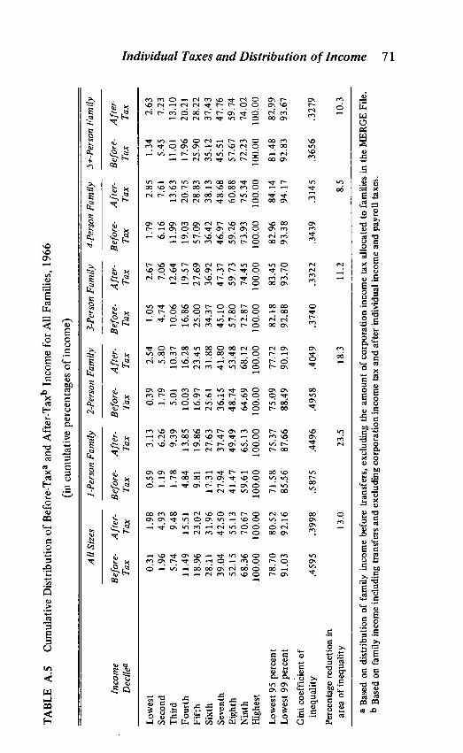
In this section, we combine the partial results discussed aboveto assess the overall impact of individual taxes and transfers on thedistribution of before-tax income. The most expeditious way tosummarize the large amount of information already presented is interms of Lorenz curves showing the various income distributions.The before-tax and after-tax and transfer Lorenz curves for allfamilies are shown in Chart 120 and the Gini coefficients andpercentage reductions in the areas of inequality for each of thepopulation subgroups examined are given in Table 9•21 (Thecumulative distributions of before- and after-tax income for allfamilies and for each of the population subgroups are given inAppendix Tables A.5 to A.7.)

For all families, the Gini coefficient computed on the basis ofthe before-tax distribution of income is .459 5; the coefficient forincome after transfer payments is .4 155; for income less transfersand income taxes, it is .3959; for income less transfers andemployment taxes combined, it is .4200; and the Gini coefficientfor the income distribution after both taxes and transfers is .3998.Translating these figures into more commonly used terms, they

20 Before-tax income for the distribution in Chart 1 is equal to F! beforetransfers and excluding the amount of corporation income tax allocated toeach family in the MERGE File. This is also the basis used for computing thebefore-tax and transfer Gmi coefficients in Table 9.

2 1 The percentage reduction in the area of inequality is equal to the ratioof the area between the before- and after-tax Lorenz curves (B) to the totalarea of inequality, i.e., the area between the line of equal distribution and thebefore-tax Lorenz curve (A). This ratio can be computed directly from theGini coefficients associated with the before- and after-tax Lorenz curves. Ifthe before-tax Gini coefficient is equal to G, and the after-tax Gini coefficientequals G', the percentage reduction in the area of inequality equal to(G - G')/G.


Cumulative100

90

80

70

60

50

40

30

20

1 0

00 10 20

Cumulative percentage of families90 100

CHART I: Comparison of the Distribution of Family Income Before andAfter Individual Taxes and Transfers, All Families, 1966

indicate that in the aggregate, income taxes are progressive;employment taxes are regressive; the totalemployment taxes is progressive; and that transfer payments arevery progressive.

In general, income before taxes and transfers is more equallydistributed among nonaged families than among those headed bysomeone age 65 or over. The group with the most unequaldistribution of before-tax income consists of aged single mdi-viduals; they are closely followed by aged couples. At the otherend of "the equality scale" are the "standard" four-person familiesheaded by a person under age 65.

Based on the changes in the area of inequality shown in Table 9,

percentage of income

30 40 50 60 70 80

of income and


TABLE 9 Gini Coefficients for the Distributions of Income Before Taxesand Transfers, Income After Transfers, and Income After Taxesand Transfers, 1966

Gini Percentage Change in Areaof Due to..

Income IncomeIncomeAfter Individual

Population Before After Taxes and Taxes andGroup Taxesc Transfers Transfers Transfers Transfers

All families .4595 .4155 .3998 9.6 13.0Nonaged famiiesd .4099 .3886 .3774 5.2 7.9

I person .5102 .4717 .4570 7.5 10.42 persons .43 10 .4059 .3919 5.8 9.13 persons .3628 .3427 .3297 5.5 9.14 persons .3385 .3255 .3126 3.8 7.65+ persons .3639 .3433 .3277 5.2 9.9

Aged famiiesd .6278 .4573 .4367 27.2 30.41 person .6799 .4263 .4097 37.3 39.72 persons .5842 .4129 .3944 29.3 32.53 persons .4598 .3744 .3595 18.6 21.84 persons .4869 .3916 .3647 19.6 25.15+ persons .4231 .3470 .3309 18.0 21.8

a The Gini coefficient of inequality is a statistical measure of overall equality orinequality in the distribution of income. It may vary between 0 (indicating perfectequality) and 1 (indicating perfect inequality). A decrease in the value therefore signifiesa more equal after-tax distribution of income and a more progressive tax structure.

b The percentage reduction in the area of inequality is equal to the ratio of the areabetween the before-tax and the after-tax (after-transfer) Lorenz curves to the total areaof inequality, i.e., the area between the line of equal distribution and the before-taxLorenz curve.

C Income before taxes is equal to family income less transfers, excluding the amountof corporation income tax allocated to families in the MERGE File.

d Families headed by an individual age 64 or under are considered nonaged; thoseheaded by an individual age 65 or over are classified as aged.

we find that transfer payments have a much greater effect on theafter-tax and transfer distribution of income than do tax pay-rnents. For all families, transfer payments account for aboutthree-quarters of the reduction in the area of inequality, whereastaxes account for one-fourth of the total change. Approximatelythe same proportions of total change are also attributable to the


effects of transfers and taxes for one-person nonaged families. Fortwo- and three-person nonaged families, about 60 percent of thetotal reduction in inequality can be attributed to transfers and 40percent to taxes; the proportions are about 50 percent each fortaxes and transfers among larger nonaged families.

Transfer payments are extremely important in reducinginequality in the distribution of income among the aged. For suchunits, transfers account for a minimum of about 80 percent of thetotal reudction in the area of inequality (among four-personfamilies) and they are responsible for 94 percent of the totalchange among single individuals over age 65. It should also benoted that the total percentage changes in inequality between thebefore-tax and the after-tax and transfer distributions for agedfamilies are all substantially larger than they are for the nonagedgroup.

CONCLUSIONS

On the basis of the data presented here, it is clear that (1) thenet effect of direct federal taxes and transfers has an importantimpact on the distribution of individual incomes in the economy;and (2) of the two parts, transfers play a far more important rolein redistributing income among families than do taxes.2 2 Sincethere have been two federal income tax reductions since 1966, it ispossible that we are understating the redistributive effects of taxesin this analysis. However, there have also been significant increasesin public assistance and Social Security benefits (plus payroll taxincreases) during the period which would tend to offset some ofthe tax reduction effects. The data needed to assess the impact ofthese changes are not available, but I do not believe that the majorconclusions would be very different if these new features weretaken into account. On balance, I would guess that taxes nowaccount for a little bit more of the total redistribution, whiletransfers account for a slightly smaller degree of redistribution.Thus, if further income redistribution is an important national

22 The major finding of a study of overall tax burdens in 1966 was thattotal taxes—federal, state, and local—are proportional to income for almost90 percent of all U.S. families. (See Joseph A. Pechman and Benjamin A.Okner, Who Bears the Tax Burden [Washington, D.C.: Brookings Institution,1974]). As a result, the total tax system had a very small effect on the overalldistribution of income.


objective, we must either adopt changes that will increase theprogressivity of existing taxes.2 3 and/or expand transfer paymentsto individuals using financing arrangements which are not regres-sive.

APPENDIX

TABLE A.1 Effective Rates of Total Individual Income Taxes Based onCensus Money Incomea by Age of Head and Family IncomeClasses, 1966

(percent)

Family In comeBefore Transfers

($000)A!!

FamiliesNonagedFamilies1'

AgedFamiliesb

3c 3.0 4.2 1.63- 5 6,0 6.6 185- 10 8.6 8.8 6.8

10- 15 10.6 10.6 10.015- 20 11.8 12.0 10.220- 25 13.1 13.4 9.525- 50 15.6 16.0 11.550- 100 24.5 25.8 6.8

100- 500 33.8 33.9 18.6500-1,000 45.5 45.5 —

• 1,000 and over 47.4 47.4 —


a Effective tax rates computed on the basis of Census money income excludingtransfers.


C Excludes families with negative income.

23 For ways to increase federal income tax progressivity, see Joseph A.Pechman and Benjamin A. Okner, "Individual Income Tax Erosion byIncome Classes," in The Economics of Federal Subsidy Programs, ACompendium of Papers submitted to the Joint Economic Committee, Part 1,General Study Papers, 92 Cong., 2 sess., 1972, pp. 13-40. Brookings Reprint230. For a discussion of measures that would reduce the regressivity ofpayroll taxes, see Joseph A. Pechman, Henry J. Aaron, and Michael K.Taussig, Social Security: Perspectives for Reform (Washington, D.C.:Brookings Institution, 1968), pp. 214-27.


TABLE A.2 Effective Rates of Total Individual Income Taxes Based onMoney Factor Income, by Age of Head and Family IncomeClasses, 1966

(percent)

Family IncomeBefore Transfers

($000)All

FamiliesNonagedFamilies0

AgedFamilies'2

0- 3b 47 53 343- 5 6.5 6.9 4.85- 10 8.8 9.0 7.6

10- 15 10.8 10.8 10.715- 20 12.1 12.2 10.8 '

20- 25 13.4 13.7 10.125- 50 16.0 16.3 12.050- 100 24.9 • 26.3 7.0

100- 500 34.6 34.7 18.6500-1,000 46.4 46.4 —

1,000 and over 47.9 47.9 —


a Families headed by an individual age 64 or under are considered nonaged; thoseheaded by an individual age 65 or over are classified as aged.

b Excludes families with negative income.


TABLE A.3 Effective Rates of Total Individual Income Taxes Based onTotal Money by Age of Head and Family IncomeClasses, 1966

(percent)

Family IncomeBefore Transfers

($000)All

FamiliesNonagedFamiliesb

AgedFamiliesb

0 3C 2.3 40 1.5

3- 5 5.9 6.5 3.65- 10 8.5 8.7 6.3

10- 15 10.5 10.5 9.315- 20 11.6 11.8 9.620- 25 12.6 12.9 9.125- 50 14.9 15.2 10.850- 100 22.1 23.2 6.6

100- 500 27.3 27.4 18.6500-1,000 32.8 32.8 —

1,000 and over 32.2 32.2 —


a Effective tax rates computed on the basis of total money receipts excludingtransfers.


C Exc'udes families with negative income.

TA

BL

E A

.4C

ombi

ned

Eff

ectiv

e R

ates

of

Indi

vidu

al I

ncom

e an

d E

mpl

oym

ent T

axes

a by

Age

of

Fam

ily H

ead

and

Size

of

Fam

ily,

by F

amily

Inc

ome

Cla

sses

, 196

6

(per

cent

)

Fam

ilyIn

com

eT

rans

fers

($00

0)

All

Fam

ilies

No

piag

ed F

amili

esb

Age

d Fa

mili

esb

All

Size

s

Fam

ily S

ize

All

Size

s

Fam

ily S

ize

All

Size

s

Fam

ily S

ize

12

34

5÷1

23

45+

12

34

51-

08.

49.

16.

98.

29.

510

.511

.513

.010

.99.

49.

910

.94.

03.

44.

34.

27.

65.

83-

512

.115

.310

.611

.711

.09.

613

.818

.413

.712

.211

.09.

66.

46.

05.

88.

111

.59.

35-

1014

.518

.215

115

.013

.611

.515

.019

.716

.415

.213

.611

.510

.38.

010

.312

.912

.711

.810

-15

15.2

18.3

17.0

16.4

14.4

12.9

15.3

20.1

17.6

16.6

14.4

12.9

12.8

8.7

12.7

14.8

15.6

13.3

15-

2015

.215

.616

.515

.815

.313

.915

.517

.617

.516

.215

.313

.912

.210

.110

.912

.817

.815

.320

-25

15.6

14.6

16.5

16.4

15.7

14.6

16.0

19.6

17.6

17.0

15.7

14.5

10.6

5.0

10.1

10.6

15.1

14.8

25-

5015

.512

.414

.316

.616

.215

.616

.017

.515

.816

.916

.015

.69.

96.

78.

313

.919

.610

.150

-10

019

.822

.217

.819

.721

.421

.021

.123

.921

.519

.921

.421

.04.

99.

64.

6d

100-

500

21.8

16.5

22.3

25.1

24.6

20.7

21.9

16.5

22.5

25.1

24.6

20.7

11.2

—10

.9—

——

500-

1,00

022

.719

.423

.223

.826

.023

.122

.719

.423

.223

.826

.023

.1—

1,00

0 an

d ov

er20

.819

.820

.323

.821

.121

.720

.819

.820

.323

.821

.121

.7—

——

——

—

All

clas

ses

15.4

16.5

16.1

16.2

15.4

14.0

16.0

18.9

17.7

16.6

15.4

14.0

9.8

6.7

9.1

12.7

15.5

13.0

a E

ffec

tive

tax

rate

s ar

e ca

lcul

ated

on

the

basi

s of

fam

ily in

com

e be

fore

tran

sfer

s, e

xclu

ding

the

amou

nt o

f co

rpor

atio

n in

com

e ta

x al

loca

ted

tofa

mili

es in

the

ME

RG

E F

ile.

bF

amili

eshe

aded

by

an in

divi

dual

age

64

or u

nder

are

con

side

red

nona

ged;

thos

e he

aded

by

an in

divi

dual

age

65

or o

ver

are

clas

sifi

ed a

s ag

ed.

CE

xclu

des

fam

ilies

with

neg

ativ

e in

com

es.

d L

ess

than

hal

f of

1 p

erce

nt.

TA

BL

E A

.5C

umul

ativ

e D

istr

ibut

ion

of B

efor

e.T

axa

and

Inco

me

for

All

Fam

ilies

, 196

6

a B

ased

on

dist

ribu

tion

of f

amily

inco

me

befo

reb

Bas

ed o

n fa

mily

inco

me

incl

udin

g tr

ansf

ers

and

(in

cum

ulat

ive

perc

enta

ges

of in

com

e)

tran

sfer

s, e

xclu

ding

the

amou

nt o

f co

rpor

atio

n in

com

e ta

x al

loca

ted

to f

amili

es in

the

ME

RG

E F

ile.

excl

udin

g co

rpor

atio

n in

com

e ta

x an

d af

ter

indi

vidu

al in

com

e an

d pa

yrol

l tax

es.

—S

Inco

me

All

Size

s1-

Pers

onFa

mily

2-Pe

rson

Fam

ily3-

Pers

onFa

mily

4-Pe

rson

Fam

ily5+

-Per

son

Fam

ily

Bef

ore-

Aft

er-

Bef

ore-

Aft

er-

Bef

ore-

Aft

er-

Bef

ore-

Aft

er-

Bef

ore.

Aft

er-

Bef

ore-

Aft

er-

Dec

ile'1

Tax

Tax

Tax

Tax

Tax

Tax

Tax

Tax

Tax

Tax

Tax

Tax

Low

est

0.31

L98

0.59

3A3

0.39

2.54

LO

S2.

671.

792.

851.

342.

63Se

cond

1.96

4.93

1.19

6.26

1.79

5.80

4.74

7.06

6.16

7.61

5.45

7.23

Thi

rd5.

7494

81.

789.

395.

0110

.37

10.0

612

.64

11.9

913

.63

11.0

113

.10

Four

th11

.49

15.5

14.

8413

.85

10.0

316

.28

16.8

619

.57

19.0

320

.75

17.9

620

.21

Fift

h18

.96

23.0

29.

8119

.86

16.9

723

.45

25.0

027

.69

57.0

928

.83

25.9

028

.22

Sixt

h28

.11

31.9

617

.31

27.6

325

.61

31.8

834

.37

36.9

236

.42

38.1

335

.12

37.4

3Se

vent

h39

.04

42.5

027

.94

37.4

736

.15

41.8

045

A0

47.3

746

.97

48.6

845

.51

47.7

6E

ight

h52

.15

55.1

341

.47

49.4

948

.74

53.4

857

8059

.73

59.2

660

.88

57.6

759

.74

Nin

th68

.36

70.6

759

.61

65.1

364

.69

68.1

272

.87

74.4

573

.93

75.3

472

.23

74.0

2H

ighe

st10

0.00

100.

0010

0.00

100.

0010

0.00

100.

0010

0.00

100.

0010

0.00

100.

0010

0.00

100.

00

Low

est 9

5 pe

rcen

t78

.70

80.5

271

.58

75.3

775

.09

77.7

282

.18

83.4

582

.96

84.1

481

.48

82.9

9L

owes

t 99

perc

ent

91.0

392

.16

85.5

687

.66

88.4

990

.19

92.8

893

.70

93.3

894

.17

92.8

393

.67

Gin

i coe

ffic

ient

of

ineq

ualit

y.4

595

.399

8.5

875

.449

6.4

958

.404

9.3

740

.332

2.3

439

.314

5.3

656

.327

9

Perc

enta

ge r

educ

tion

inar

ea o

f in

equa

lity

13.0

23.5

18.3

11.2

8.5

10.3

In c

ome

Dec

ile'2

Al!

S

Bef

ore-

Tax

b

izes A

fter

-T

axC

1-Pe

rson

Bef

ore-

Tax

Fam

ily

Aft

er-

Tax

2-Pe

rson

Bef

ore-

Tax

Fam

ily

Aft

er-

Tax

3-Pe

rson

Bef

ore-

Tax

Fam

ily

Aft

er-

Tax

4-Pe

rson

Bef

ore.

Tax

Fam

ily

Aft

er-

Tax

5+-P

erso

Bef

ore-

Tax

n Fa

mily

Aft

er-

Tax

Low

est

0.78

1.85

0.49

1.81

0.92

2.04

1.42

265

1.99

2.88

1.41

2.64

Seco

nd3.

915.

4816

64.

113.

995.

835.

477.

156.

487.

7155

97.

29T

hird

8.83

10.6

64.

587.

778.

7711

.02

10.9

612

.88

12.4

013

.80

11.1

813

.17

Four

th15

.16

17.1

49.

4213

.08

14.9

417

.39

17.8

419

.91

1943

20.9

118

.12

20.2

6Fi

fth

22.9

524

.95

16.1

519

.97

22.3

124

.84

25.9

528

.07

27.4

829

.00

26.0

428

.27

Sixt

h31

.95

33.9

524

.77

28.4

830

.95

33.4

635

.20

37.2

736

.80

38.3

135

.23

3745

Seve

nth

42.4

844

.38

35.0

838

.41

40.7

543

.09

45.7

147

.59

47.2

948

.83

45.5

847

73E

ight

h54

.79

56.5

447

.86

50.4

952

.41

54.5

058

.12

59.7

759

4760

.95

57.6

959

.69

Nin

th69

.92

71.4

463

.64

65.4

966

.71

68.4

172

.87

74.2

074

.00

75.3

372

.20

73.9

4H

ighe

st10

0.00

100.

0010

0.00

100.

0010

0.00

100.

0010

0.00

100.

0010

0.00

100.

0010

0.00

100.

00

Low

est 9

5 pe

rcen

t79

.44

80.7

473

.76

75.0

675

.81

77.2

581

.99

83.1

082

.98

84.0

581

.44

82.9

2L

owes

t 99

perc

ent

91.0

691

.99

85.2

386

.04

88.7

489

.81

92.6

193

.37

93.3

394

.11

92.8

493

.65

Gin

i coe

ffic

ient

of

ineq

ualit

y.4

099

.377

4.5

102

.457

0.4

310

.391

9.3

628

.329

7.3

385

.312

6.3

639

.327

7

Perc

enta

ge r

educ

tion

inar

ea o

f in

equa

lity

7.9

10.4

9.1

9.1

7.7

9.9

a B

ased

on

dist

ribu

tion

of f

amily

inco

me

befo

re tr

ansf

ers,

exc

ludi

ng th

e am

ount

of

corp

orat

ion

inco

me

tax

allo

cate

d to

fam

ilies

in th

e M

ER

GE

File

.B

ased

on

fam

ily in

com

e in

clud

ing

tran

sfer

s an

d ex

clud

ing

corp

orat

ion

inco

me

tax

and

afte

r in

divi

dual

inco

me

and

payr

oll t

axes

.C

Fam

ilies

head

ed b

y an

indi

vidu

al a

ge 6

4 or

und

er.

TA

BL

E A

.6C

umul

ativ

e D

istr

ibut

ions

of

Bef

ore.

Tax

a an

d A

fter

-Tax

for

Non

aged

' Fam

ilies

, 196

6

(in

cum

ulat

ive

perc

enta

ges

of in

com

e)

I

TA

BL

E A

.7C

umul

ativ

e D

istr

ibut

ions

of

and

Aft

er-T

ax I

ncom

esb

for

Age

d Fa

rnili

es,C

196

6

(in

cum

ulat

ive

perc

enta

ges

of in

com

e)

.

Inco

me

All

Size

s1-

Pers

onFa

mily

2-Pe

rson

Fam

ily3-

Pers

onFa

mily

4-Pe

rson

Fam

ily5+

-Per

son

Fam

ily

Bef

ore-

Aft

er.

Bef

ore-

Aft

er-

Bef

ore-

Aft

er-

Bef

ore.

Aft

er.

Bef

ore.

Aft

er.

Bef

ore.

Aft

er.

Decilea

Tax

Tax

Tax

Tax

Tax

Tax

Tax

Tax

Tax

Tax

Tax

Tax

Low

est

0.69

3.48

1.09

4.68

0.77

3.78

0.53

2.83

0.26

2.78

0.39

2.70

Seco

nd1.

397.

002.

189.

361.

547.

621.

536.

061.

55•6

.22

2.32

6.12

Thi

rd2.

0810

.52

3.27

14.0

52.

8911

.83

4.24

10.4

84.

3211

.08

5.86

11.3

2Fo

urth

3.73

14.7

34.

3618

.73

5.76

17.0

49.

3916

.70

8.88

16.7

210

.88

17.2

7Fi

fth

7.30

20.3

55.

4523

.42

10.2

723

.52

16.0

923

.75

14.9

923

.80

18.7

325

.53

Sixt

h13

.25

27.6

59.

4529

.69

17.1

831

.38

25.8

233

.24

23.5

932

.69

28.7

135

.41

Seve

nth

22.0

536

.98

17.0

738

.06

26.6

941

.16

38.5

544

.74

34.6

943

.34

42.1

247

.99

Eig

hth

35.5

749

.38

29.0

148

.99

40.0

553

.02

54.2

458

.93

50.3

957

.77

56.8

662

.33

Nin

th56

.77

66.4

848

.11

64.3

459

.27

68.2

572

.99

76.0

771

.03

75.8

174

.94

78.1

1H

ighe

st10

0.00

100.

0010

0.00

100.

0010

0.00

100.

0010

0.00

100.

0010

0.00

100.

0010

0.00

100.

00

Low

est 9

5 pe

rcen

t72

.60

78.9

263

.97

75.8

773

.08

79.0

784

.27

86.3

284

.39

87.0

786

.35

88,0

0L

owes

t 99

perc

ent

91.0

193

.01

87.2

191

.60

90.9

092

.89

95.9

896

.40

96.4

596

.91

96.4

896

.95

.G

ini c

oeff

icie

nt o

fin

equa

lity

.628

7.4

367

.679

9.4

097

.584

2.3

944

.459

8.3

595

.486

9.3

647

.423

1.3

309

Perc

enta

ge r

educ

tion

inar

ea o

f in

equa

lity

30.5

39.7

32.5

21.8

25.1

21.8

a B

ased

on

dist

ribu

tion

of f

amily

inco

me

befo

re tr

ansf

ers,

exc

ludi

ng th

e am

ount

of

corp

orat

ion

inco

me

tax

allo

cate

d to

fam

ilies

in th

e M

ER

GE

File

.b

Bas

ed o

n fa

mily

inco

me

incl

udin

g tr

ansf

ers

and

excl

udin

g co

rpor

atio

n in

com

e ta

x an

d af

ter

indi

vidu

al in

com

e an

d pa

yrol

l tax

es.

CF

amili

eshe

aded

by

an in

divi

dual

age

65

or o

ver.

Individual Taxes and the Distribution of Income 3 Individual Taxes and the Distribution of Income...

Documents

Transcript of Individual Taxes and the Distribution of Income 3 Individual Taxes and the Distribution of Income...