Individual Preferences for Giving∗

Raymond Fisman†

Columbia UniversityShachar Kariv‡

UC BerkeleyDaniel Markovits§

Yale University

November 1, 2005

AbstractThis paper reports an experimental test of individual preferences for

giving. We use graphical representations of modified Dictator Gamesthat vary the price of giving. This generates a very rich data setwell-suited to studying behavior at the level of the individual subject.We test the data for consistency with preference maximization, andwe recover underlying preferences and forecast behavior using bothnonparametric and parametric methods. Our results emphasize thatclassical demand theory can account very well for behaviors observedin the laboratory and that individual preferences for giving are highlyheterogeneous, ranging from utilitarian to Rawlsian to perfectly selfish.(JEL: C79, C91, D64)

∗This research was supported by the Experimental Social Science Laboratory (X-Lab)at the University of California, Berkeley. We thank Jim Andreoni and Gary Charness fordetailed comments and suggestions. We are also grateful to Colin Camerer, Ken Chay,Stefano DellaVigna, Steve Goldman, Botond Koszegi, John List, Tom Palfrey, Ben Polak,Jim Powell, Matthew Rabin, Al Roth, Ariel Rubinstein, Chris Shannon, Andrew Schotterand Hal Varian for helpful discussions. This paper has also benefited from suggestions bythe participants of seminars at several universities. Syngjoo Choi and Benjamin Schneerprovided excellent research assistance. In addition, we would like to thank Brenda Naputiand Lawrence Sweet from the X-Lab for their valuable assistance, and Roi Zemmer forwriting the experimental computer program. For financial support, Fisman thanks theColumbia University Graduate School of Business; Kariv acknowledges University of Cal-ifornia, Berkeley; Markovits thanks Yale Law School and Deans Anthony Kronman andHarold Koh.

†Graduate School of Business, Columbia University, Uris 823, New York, NY 10027(E-mail: rf250@columbia.edu, URL: http://www-1.gsb.columbia.edu/faculty/rfisman/).

‡Department of Economics, University of California, Berkeley, 549 EvansHall # 3880, Berkeley, CA 94720 (E-mail: kariv@berkeley.edu, URL:http://socrates.berkeley.edu/~kariv/).

§Yale Law School, P.O. Box 208215, New Haven,CT 06520. (E-mail: daniel.markovits@yale.edu, URL:http://www.law.yale.edu/outside/html/faculty/ntuser93/profile.htm)

1

1 Introduction

We study individual preferences for giving. We emphasize the term individ-ual to highlight that we will investigate behavior at the level of the individualsubject. Our experiment employs a modified dictator game that varies theendowments and the prices of giving, so that each subject faces a menu ofbudget sets over his own payoff and the payoff of one other subject. Weintroduce a graphical computer interface that allows for the efficient col-lection of many observations per subject. Given our rich data set, we canthoroughly address four types of questions concerning preferences for giv-ing (Varian 1982): (i) Consistency. Is behavior consistent with the utilitymaximization model? (ii) Recoverability. Can underlying preferences berecovered from observed choices? (iii) Extrapolation. Can behavior on pre-viously unobserved budget sets be forecasted? (iv) Heterogeneity. To whatdegree do preferences differ across subjects?

The importance of studying individual heterogeneity is emphasized byAndreoni and Miller (2002) (hereafter AM), who also ask whether behavioris consistent with the utility maximization model by applying the axiomof revealed preference. AM report that classical demand theory is indeedrelevant to the interpretation of the experimental data and that preferencesare very heterogeneous. Because of this heterogeneity, AM conclude that itis necessary to investigate behavior at an individual level. However, theirexperimental design involves few budgets sets and allows for only a smallnumber of decisions per subject, which necessitates the pooling of obser-vations across subjects. Our experimental design allows subjects to makenumerous choices over a wide range of budget sets, and this yields a richdataset that is well-suited to analysis at the level of the individual subject.

We begin our analysis of the experimental data by testing for consis-tency with utility maximization using revealed preference axioms. Afriat(1967) shows that if finite choice data satisfy the Generalized Axiom of Re-vealed Preference (GARP), there exists a well-behaved utility function thatthe choices maximize. Varian (1982) modifies Afriat’s (1967) results anddescribes the most efficient and general techniques for testing the extent towhich choices satisfy GARP. Since GARP offers an exact test (i.e. eitherthe data satisfy GARP or they do not) and choice data almost always con-tain at least some violations, we calculate a variety of goodness-of-fit indicesdescribed by Varian (1991) to quantify the extent of violation. We find thatmost subjects exhibit behavior that appears to be almost optimizing in thesense that their choices nearly satisfy GARP, so that the violations are minorenough to ignore for the purposes of recovering preferences or constructing

2

appropriate utility functions.We therefore move to recovering underlying preferences and forecasting

behavior in new situations. We begin by using the revealed preference tech-niques developed by Varian (1982). This approach is purely nonparametricand compares arbitrary allocations or budgets assuming only consistencywith previously observed behavior and making no assumptions about theparametric form of the underlying utility function. Because of our rich dataset, we are able to generate fairly tight bounds on these measures. Weconduct case studies of several subjects that almost satisfy GARP and whoserve to illustrate ideal types whose choices fit with prototypical preferences.

Motivated by patterns observed in the nonparametric approach, we esti-mate constant elasticity of substitution (CES) demand functions for givingat the individual level. The CES form is very useful in many applicationssince it spans a range of well-behaved utility functions by means of a sin-gle parameter. We find that the CES demand function provides a goodfit at the individual level. Moreover, the parameter estimates vary dramati-cally across subjects, implying that individual preferences for giving are veryheterogeneous, ranging from perfect substitutes to Leontief. However, likeCharness and Rabin (2002), we do find that a significant majority of sub-jects are concerned with increasing aggregate payoffs rather than reducingdifferences in payoffs.

Our paper contributes to the large and growing body of work that seeksto explain departures from self-interest in economic experiments. Socialpreferences theories include altruism, relative income and envy, inequalityaversion, and altruism and spitefulness (see, respectively, Charness and Ra-bin (2002), Bolton (1991), Levine (1998) and Fehr and Schmidt (1999),among others). Our paper provides a couple of fundamental innovationsover previous work. Most importantly, previous experimental studies haveinferred preferences from a small number of individual decisions and hencehave been forced to set up relatively extreme choice scenarios. In contrast,we do not force subjects into choices that suggest discrete and extreme pro-totypical preference types. This enables us to analyze preferences for givingat the individual level. This is crucial. As AM emphasize, individual het-erogeneity requires behavior to be examined at an individual level, beforepreferences can properly be understood. Our primary methodological con-tribution is an experimental technique that enables us to collect richer dataabout preferences for giving than has heretofore been possible. The exper-imental techniques and our results provide promising tools for future workin this area.

The rest of the paper is organized as follows. The next section describes

3

the experimental design and procedures. Section 3 summarizes some impor-tant features of the data. Section 4 provides the nonparametric analysis,and Section 5 provides the parametric analysis. Section 6 concludes. Theexperimental instructions are reproduced in Section 7.

2 Experimental design and procedures

2.1 Design

We begin by discussing a very general formulation of the dictator game,before outlining the linear version that we utilize in our experiments. Weadopt AM’s notation and model a generalized dictator game by a set of twopersons s and o (s for self and o for other), a compact subset of the planeΠ representing the feasible monetary payoff choices of person s (i.e. eachpoint π = (πs, πo) in Π corresponds to the payoffs to persons self and other,respectively), and a preference ordering %sfor person s. For any π, π0 ∈ Π,π %s π0 if and only if person s prefers π to π0 or is indifferent betweenthem. The preference ordering %scan be represented by a utility functionUs = us(πs, πo) that captures the possibility of giving if us(π) ≥ us(π

0)whenever π %s π

0. Person s is said to be selfish, or an own-payoff maximizer,when π %s π0 if and only if πs ≥ π0s. The objects s,Π and %s define thedictator game.

The set Π of feasible payoff pairs may take many forms and one shouldultimately put no restrictions directly on Π. Yet, in a typical dictator ex-periment, first introduced by Forsythe, et al. (1994), subject s divides someendowment m between self and other in any way he wishes such that

Π = {(πs, πo) : πs + πo = m}.

One respect in which this framework is restrictive is that the set Π is alwaysthe line with a slope of −1 so the problem faced by person s is simplyallocating a fixed total income between self and other.

A full generalization of the dictator game would allow for nonlinear bud-get sets. But because a great deal of classical theory is built on the assump-tion of a simple linear budget constraint, the simplest and perhaps mostimportant generalization of the dictator game, developed by AM, allows foran endowment which is to be spent on πs and πo at given fixed correspond-ing price levels ps and po. By choosing ps as the numeraire price, the set ofnormalized possible payoffs for the game can then be written

Π = {(πs, πo) : πs + pπo = m0}

4

where p = po/ps is the relative price of giving and m0 = m/ps. This configu-ration creates budget sets over πs and πo that allow for the thorough testingof observed dictator behavior for consistency with utility maximization.1

2.2 Procedures

The experiment was conducted at the Experimental Social Science Labo-ratory (X-Lab) at the University of California, Berkeley under the X-LabMaster Human Subjects Protocol.2 The 76 subjects in the experiment wererecruited from all undergraduate classes at UC Berkeley and had no pre-vious experience in experiments of dictator, ultimatum, or trust games.After subjects read the instructions, the instructions were read aloud byan experimenter. The experimental instructions build on AM with minorchanges to reflect employment of computers (see Section 7). At the end ofthe instructional period subjects were asked if they had any questions or anydifficulties understanding the experiment. No subject reported any difficultyunderstanding the procedures or using the computer program. Each exper-imental session lasted for about one and a half hours. A $5 participationfee and subsequent earnings, which averaged $16, were paid in private atthe end of the session.3 Throughout the experiment we ensured anonymityand effective isolation of subjects in order to minimize any interpersonalinfluences that could stimulate other-regarding behavior.4

Each session consisted of 50 independent decision-problems. In each de-cision problem, each subject was asked to allocate tokens between himselfπs and an anonymous subject πo, where the anonymous subject was chosenat random from the group of subjects in the experiment. Each choice in-volved choosing a point on a graph representing a budget set over possibletoken allocations. Each decision problem i = 1, ..., 50 started by having thecomputer select a budget set randomly from the set

{pisπs + pioπo ≤ mi : mi/pn ≤ 100 for both n = s, oand mi/pn ≥ 50 for some n = s, o}

1Andreoni and Vesterlund (2001) utilize the same design as AM to study whetherpreferences for giving differ by gender. They find that men are more responsive to pricechange and likely to be either perfectly selfish or utilitarian, whereas women tend to beRawlsian.

2See http://xlab.berkeley.edu/cphs/master_protocol.pdf.3Payoffs were calculated in terms of tokens and then translated at the end of the

experiment into dollars at the rate of 3 tokens = 1 dollar.4Subjects’ work-stations were isolated by cubicles making it impossible for subjects to

observe other screens or to communicate.

5

(i.e. budget sets that intersect with at least one of the axes at 50 ormore tokens, but with no intercept exceeding 100 tokens). For compari-son, in AM, the full menu of budgets offered included only 8 budget con-straints in four sessions and 11 in one session with m = {40, 60, 75, 100} andp = {1/4, 1/3, 1/2, 1, 2, 3, 4}. The sets selected for each subject in differentdecision problems were independent of each other and of the sets selectedfor any of the other subjects in their decision problems. Notice that choiceswere not restricted to allocations on the budget constraint so that, in theory,subjects could costlessly dispose payoffs and violate budget balancedness (i.e.piπi = mi).

To choose an allocation, subjects used the mouse or the arrows on thekeyboard to move the pointer on the computer screen to the desired allo-cation. Subjects could either left-click or press the Enter key to make theirallocation. At any point, subjects could either right-click or press the Spacekey to find out the allocation at the pointer’s current position. The πs-axisand πo-axis were labeled Hold and Pass respectively and scaled from 0 to100 tokens. The resolution compatibility of the budget sets was 0.2 tokens;the sets were colored in light grey; and the frontiers were not emphasized.The graphical representation of budget sets also enabled us to avoid empha-sizing any particular allocation. At the beginning of each decision round,the experimental program dialog window went blank and the entire setupreappeared. The appearance and behavior of the pointer were set to theWindows mouse default and the pointer was automatically repositioned atthe origin π = (0, 0) at the beginning of each round.

This process was repeated until all 50 rounds were completed. At theend of the experiment, payoffs were determined in the following way. Theexperimental program first randomly selected one decision round from eachsubject to carry out. That subject then received the tokens that he heldin this round πs, and the subject with whom he was matched received thetokens that he passed πo. Thus, as in AM, each subject received two groupsof tokens, one based on his own decision to hold tokens and one based on thedecision of another random subject to pass tokens. The computer programensured that the same two subjects were not paired twice. Subjects receivedtheir payment privately as they left the experiment.

The experiments provide us with a very rich dataset. We have observa-tions on 76×50 = 3800 individual decisions over a variety of different budgetsets. Most importantly, the broad range of budget sets provides a serioustest of the ability of classical theory, and a structural econometric modelbased on the theory, to interpret the data. In particular, the changes inendowments and relative prices are such that budget lines cross frequently.

6

This means that our data lead to high power tests of revealed preferenceconditions (see Varian (1982), Bronars (1987), Russell (1992) and Blundell,Browning and Crawford (2003)).

Aside from pure technicalities, our paper provides a couple of importantinnovations over previous work. First it allows us to test a wider rangeof budget sets than can be tested using the pencil-and-paper experimentalquestionnaire method of AM. Second, it generates a rich dataset that pro-vides the opportunity to address recoverability and extrapolation at the levelof the individual subject. This is particularly important. As AM emphasize,individual heterogeneity requires behavior to be examined at an individuallevel, before preferences can properly be understood.

3 Overview of experimental data

In this section, we provide an overview of some important features of theexperimental data, which we summarize by reporting the distribution ofallocations in a number of ways. The histograms in Figure 1 show the dis-tributions of the fraction given to other, defined in a couple of ways. Figure1A depicts the distribution of the expenditure on tokens given to other pioπ

io

as a fraction of total expenditure pisπis + pioπ

io, or simply

piπioπis + piπio

,

and Figure 1B depicts the distribution of the tokens given to other as afraction of the sum of the tokens kept and given

πioπis + πio

.

Clearly, this distinction is only relevant in the presence of price changes.Further, in each case we present the distribution for all allocations, as wellas the distributions by three price terciles: intermediate prices of around1 (0.70 ≤ p ≤ 1.43), steep prices (p > 1.43) and symmetric flat prices(p < 0.70). The horizontal axis measures the fractions for different intervalsand the vertical axis measures the percentage of decisions corresponding toeach interval.

[Figure 1 here]

In Figure 1A, for the full sample there is a mode at the midpoint of 0.5(i.e. same expenditure on self and other, pisπ

is = pioπ

io). The number of

7

allocations then decreases as we move to the left, before increasing rapidlyto selfish allocations of 0.05 or less of the total expenditure on tokens forother, which account for 40.5 percent of all allocations. This masks someheterogeneity by price. For the middle tercile, the pattern is somewhatmore pronounced, while for the flat tercile, there is no peak at the midpoint.Not surprisingly, the distribution is generally further to the left for steeper-sloped budgets. Figure 1B shows a similar pattern to Figure 1A, though itis somewhat more skewed to the left. Compared with studies of split-the-piedictator games (See, Camerer (2003) for a comprehensive discussion), themode at the midpoint is relatively less pronounced and the distribution ismuch smoother, even for the intermediate tercile allocations. Over all prices,our subjects gave to other about 19 percent of the tokens, accounting for 21percent of total expenditure; this is very similar to typical mean allocationsof about 20 percent in the studies reported in Camerer (2003).

The decision-level graphs in Figure 1 potentially obscure the presence ofindividual concerns on average for others. For example, a person who giveseverything to other half of the time and keeps everything for self the otherhalf would generate extreme giving values, when in fact such a person keepsan intermediate fraction on average. Hence, Figure 2 shows the distributionof piπio/(π

is + piπio) presented in Figure 1A aggregated to the subject level.

Since this takes an average over all prices, the distribution should be similarfor πi/(πis+πio) (in practice, the histograms are identical once we aggregateby decile). The horizontal axis measures the fractions for different intervalsand the vertical axis measures the percentage of subjects corresponding toeach interval. Perhaps as expected, the distributions show a pattern with alarger mode around the midpoint and no observations below the midpoint.

[Figure 2 here]

These aggregate distributions tell us little about the particular alloca-tions chosen by individual subjects. As a preview, Figure 3 shows the scat-terplot of the choices made by subjects whose choices correspond to proto-typical preferences. Figure 3A depicts the choices of a selfish subject (ID4) U(πs, πo) = πs, Figure 3B depicts the allocations of a subject with util-itarian preferences (ID 54) U(πs, πo) = πs + πo, and Figure 3C depicts theother extreme, that of a Rawlsian subject (ID 46) U(πs, πo) = min{πs, πo}.Of our 76 subjects, 20 (26.3 percent) behaved perfectly selfishly. Only two(2.6 percent) subjects allocated all their tokens to self if ps < po and toother if ps > po implying utilitarian preferences, and two (2.6 percent) sub-jects made nearly equal expenditure on self and other indicating Rawlsian

8

preferences. By comparison, AM report that 40 subjects (22.7 percent) be-haved perfectly selfishly, 25 subjects (14.2 percent) could fit with utilitarianpreferences, and 11 subjects (6.2 percent) were consistent with Rawlsianpreferences. We also find many intermediate cases, but these are difficult tosee directly on a scatterplot due to the fact that both p and m shift in eachnew allocation. This is the purpose of our individual-level analysis below.

[Figure 3 here]

4 Nonparametric analysis

4.1 Consistency

Varian (1982) describes a set of techniques, based on revealed preferenceaxioms, through which to test a finite set of data for consistency with utilitymaximization, to recover preferences from the data, and to forecast demandbehavior on budget sets which have not been previously observed.

Let (pi, πi) for i = 1, ..., n be some observed individual data (i.e. pi

denotes the ith observation of the prices and πi denotes the associated al-location). Throughout this section it will be convenient to normalize theprices, pis and p

io, by the endowment m

i at each observation so that piπi = 1for all i.

First, we recall that πi is directly revealed preferred to π if piπi ≥ piπand strictly directly revealed preferred if the inequality is strict. The relationindirectly revealed preferred is the transitive closure of the directly revealedpreferred relation. We then define the following:

Generalized Axiom of Revealed Preference (GARP) If πi is indirectlyrevealed preferred to πj , then πj is not strictly directly revealed pre-ferred (i.e. pjπi ≥ pjπj) to πi.

A utility function us(π) rationalizes the observed behavior if us(πi) ≥us(π) for all π such that piπi ≥ piπ (i.e. us achieves the maximum on thebudget set at the chosen bundle). GARP is tied to utility representationthrough the following theorem, which was first proved by Afriat (1967):

Afriat’s Theorem The following conditions are equivalent: (i) The datasatisfy GARP. (ii) There exists a non-satiated utility function thatrationalizes the data. (iii) There exists a concave, monotonic, contin-uous, non-satiated utility function that rationalizes the data.5

5This statement of the theorem follows Varian (1982), who replaced the conditionAfriat called cyclical consistency with GARP.

9

The equivalence of (i) and (ii) establishes GARP as a direct test forwhether a finite data set may be rationalized by a utility function, and theequivalence of (ii) and (iii) tells us that when a rationalizing utility functionexists, it can be chosen to be well-behaved.

In order to verify that the data satisfies GARP it is only necessary tohave an efficient way to compute the transitive closure of a binary relation.A variety of easily implementable graph theoretic algorithms, such as thatdescribed in Varian (1982), provide an efficient way to check GARP bycomputing the transitive closure of the directly revealed preference relation.

To better understand our measures of consistency, it is instructive todescribe the basic idea underlying the algorithm (the computer programand details are available from the authors upon request). Consider a directedgraph G with a set of nodes

V = {1, ..., n}

and set of edgesE = ∪ni=1{ij : piπi ≥ piπj}.

That is, the graph is a pair G = (V,E) of sets satisfying E ⊆ [V ]2 withnodes representing individual decisions and edges representing directly re-vealed preferred relations. Note that the edges need not be symmetric: theexistence of an edge directed from i to j does not imply the existence of anedge from j to i (in fact, this would imply a GARP violation if one of theinequalities were strict).

For any nodes i and j, an i − j path is a finite sequence i1, ..., iK suchthat i1 = i, iK = j and pkπk ≥ pkπk+1 for k = 1, ...,K − 1 (i.e. a sequenceof nodes i1, ..., iK linked by E). Note that a path represents a revealedpreferred relation in the data (i.e. πi is revealed preferred to πj if and onlyif there exists an i − j path). A cyclic sequence of nodes that creates ani − i path called a cycle. The length of a cycle is its number of edges, anda cycle of length k is called a k-cycle. It follows directly from the definitionthat if G contains a cycle with at least one strict inequality, then we havea violation of GARP. The number of cycles in G is the number of GARPviolations.

4.2 Goodness-of-fit

As formulated above, GARP offers an exact test: either the data satisfyGARP and are therefore consistent with the utility maximization model, orthey do not. Unfortunately, choice data almost always contain at least some

10

violations. Hence, it is useful to measure the extent of GARP violation. Wereport measures of GARP violation based on three indices: Afriat (1972),Houtman and Maks (1985), and Varian (1991) which we refer to as theE-index, V -index and EV -index, respectively, according to whether theyinvolve conditions on edges, vertices, or both.

The first index is what Afriat (1972) calls the critical cost efficiency index(CCEI); it measures the amount by which each budget constraint must berelaxed in order to remove all violations of GARP. More precisely, let (ei)be a vector of numbers with 0 ≤ ei ≤ 1. Define G0 to be a spanning subgraphof G (i.e. G0 = (V 0, E0) with V 0 = V and E0 ⊆ E) with

E0 = ∪ni=1{ij : eipiπi ≥ piπj}.

Then the CCEI is the largest number ei such that the subgraph G0 does notcontain any cycle, with at least one of the inequalities holding strictly. Wecall this number the E-index. Note that the E-index provides a summarystatistic of the overall consistency of the data with GARP but gives no hintas to which of the observations are causing violations. Figure 4 illustratesthe construction of the E-index for a simple violation of GARP.6 Note thata small perturbation A/B < C/D of the budget constraint through obser-vation π0 removes the violation.

[Figure 4 here]

The second test, proposed by Houtman and Maks (1985), finds thelargest subset of choices that is consistent with GARP. More formally, letG00 be an induced subgraph of G (i.e. G00 = (V 00, E00), with V 00 ⊆ V and E00

containing all edges ij ∈ E with i, j ∈ V 00) and find the graph G00 with thelargest order |G00| (i.e. number of nodes) that does not contain any cycle. Wecall the ratio |G00| / |G| the V -index; note that |G00| / |G| ∈ [0, 1], with highernumbers reflecting a larger subset of consistent observations. This methodhas a couple of drawbacks. First, observations may be discarded even if theassociated GARP violations could be removed by small perturbations of thebudget constraint. Further, it is computationally very intensive and thusimpractical if, roughly speaking, cycles often overlap. As a result, we wereunable to calculate the V -indices for a small number of subjects who oftenviolated GARP, and we therefore report only lower bounds.

6Here we have a violation of the Weak Axiom of Revealed Preference (WARP) (i.e. πi

is directly revealed preferred to πj 6= πi and πj is directly revealed preferred to πi).

11

The third test follows Varian (1991), who refined the E-index (Afriat’sCCEI) by providing a more disaggregated measure that indicates the min-imal amount required to perturb each observation in order to remove allviolations of GARP. With a slight abuse of notation, let (vi) be a vector ofnumbers with 0 ≤ vi ≤ 1. Let G000 be a spanning subgraph of G with

E000 = ∪ni=1{ij : vipiπi ≥ piπj}.

Then, vi is the largest number such that the subgraph G000 does not containany i− i cycles, with at least one of the inequalities holding strictly. Thus,vi = 1 if and only if G does not contain an i− i cycle. Note that (vi) neednot be the smallest perturbation of the data that is consistent with GARPbecause an i−i cycle may often be broken by perturbing an edge which joinstwo other nodes of the cycle. To describe efficiency, Varian (1991) uses thesmallest (vi), which we call EV -index. Note that the EV -index is a lowerbound on the E-index. The reasons for this discrepancy are discussed inVarian (1991).

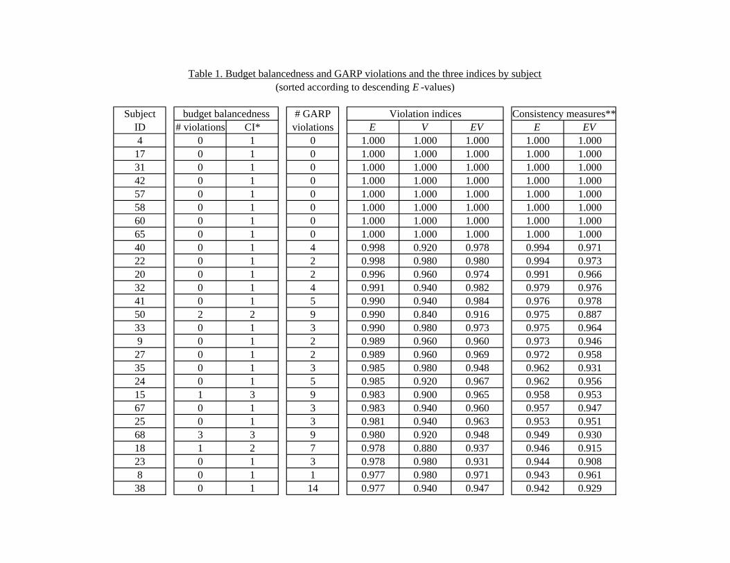
Table 1 lists, by subject, the number of violations of budget balanced-ness and GARP, and also reports the three indices according to descendingE-values. We need to allow for small mistakes resulting from the slight im-precision of subjects’ handling of the mouse. The results presented in Table1 allow for a narrow confidence interval of one token (i.e. for any i and j 6= i,if d(πi, πj) ≤ 1 then πi and πj are treated as the same allocation).

[Table 1 here]

Half of our subjects have no violations of budget balancedness, evenwith the narrow one token confidence interval; if we allow for a five tokenconfidence interval, 64 subjects (84.2 percent) have no violations of budgetbalancedness. The second column of Table 1 reports the confidence intervalrequired to remove all budget balancedness violations.7

Turning now to GARP violations, out of the 76 subjects, only 8 (10.5percent) have no violations of GARP, but all of these are subjects that al-ways chose selfish allocations πi = (mi/pis, 0) for all i. However, 54 subjects,(71.1 percent) had E-indices above the 0.90 threshold, and of those 41 sub-jects (53.9 percent) were above the 0.95 threshold. In contrast, AM reportthat only 18 of their 176 subjects (10.2 percent) violated GARP, and ofthose only 3 had E-indices below the 0.95 threshold. This is as expected,

7We note that there are a few subjects that required large confidence intervals, but thatthese subjects also have many GARP violations even if the choices that violate budgetbalancedness are removed.

12

as our subjects were given a larger and richer menu of budget sets whichprovides more opportunities to violate GARP and thus improves the powerof nonparametric tests of revealed preference theory. Figure 5 shows the dis-tributions of the three indices. The horizontal axis measures the indices fordifferent intervals and the vertical axis measures the percentage of subjectscorresponding to each interval.

[Figure 5 here]

Nonetheless, we argue that most of our subjects are close enough topassing GARP so that we may not want to reject that their choices are con-sistent with utility maximization. To give greater precision to this notion,we wish to generate a benchmark levels of consistency with which we maycompare our E-index and EV -index. As in AM, we use the test designed byBronars (1987) that uses the choices of a hypothetical subject who random-izes uniformly among all allocations on each budget line as a benchmark.To this end, we generated a random sample of 25,000 subjects and foundthat all of them violated GARP. Their E-index and EV -index values aver-aged 0.60 and 0.25 respectively.8 If we choose the 0.9 efficiency level as ourcritical value, we find that only 12 of the random subjects’ E-index valueswere above the threshold and none of the subjects’ EV -index values wereabove this threshold. Using the same approach on only 8 random budgetsets, which is the number of decisions made by most of AM’s subjects, wefind that random decisions generate average E-index and EV -index valuesof 0.91 and 0.78 respectively.9

In order to determine the extent to which subjects are consistent withGARP relative to random allocations, for each subject we take the differ-ence between his actual index and the average random-choice index as afraction of the difference between consistent-choice index of one and the av-erage random-choice index. We do this for both the E-index and EV -index.Subjects with no GARP violations have a consistency of one and the av-erage random subject has a consistency of zero; obviously, negative valuesare possible if a subject performs worse than randomness. The results arepresented in the final two columns of Table 1 above, and illustrated in the

8Note that we cannot generate an average V -index for random subjects because of thecomputational complexity required.

9Bronars’ test (i.e. the probability that a random subject violates GARP) has also beenapplied to experimental data by Cox (1987), Sippel (1997), Mattei (2001) and Harbaugh,Krause and Berry (2001). Our study has the highest Bronar power of one (i.e. all randomsubjects had violations).

13

histograms of consistency values in Figure 6. As Figure 6 shows, the dis-tribution of consistency values is skewed to the right and almost uniformlypositive; this provides a clear graphical illustration of the extent to whichsubjects did worse than choosing consistently and the extent to which theydid better than choosing randomly.

[Figure 6 here]

Finally, notice that subjects in our experiment could not exhibit suchalmost-optimizing behavior if they had any difficulties understanding thedecision problem or using the computer program. Also, the fact that choicesnearly satisfy GARP implies that subjects had to exhibit stable patterns ofchoices over the course of the experiment.

4.3 Recovering preferences and forecasting behavior

If choice data satisfy GARP we would ideally like to extract a rationalizingutility function through which to recover preferences and forecast choiceson out-of-sample allocations. Varian (1982) uses GARP and assumptionsof convexity and monotonicity to generate an algorithm that serves as apartial solution to this so-called recoverability problem. This algorithm canalso recover preferences from choices, such as the ones in our experiment,that are almost consistent with GARP. Further, since we observe manychoices over a wide range of budget sets, we can describe preferences withsome precision.

We give a brief outline of Varian’s algorithm, which provides the tightestpossible bounds on indifference curves through an allocation π0 that has notbeen observed in the previous data (pi, πi) for i = 1, ..., n. First, we considerthe set of prices at which π0 could be chosen and be consistent (i.e. doesnot add violations of GARP) with the previously observed data. This setof prices is the solution to the system of linear inequalities constructed fromthe data and revealed preference relations. Call this set S(π0). Second, weuse S(π0) to generate the set of observations, RP (π0), revealed preferred toπ0 and the set of observations, RW (π0), revealed worse than π0.

It is not difficult to show that RP (π0) is simply the convex monotonichull of all allocations revealed preferred to π0. To understand the construc-tion of RW (π0), note that if π0 is directly revealed preferred to some ob-servation πi for all prices p0 ∈ S(π0) (i.e. p0π0 ≥ p0πi), then it is indirectlyrevealed preferred to any allocation in the budget set (pi, 1) on which πi waschosen. Similarly, it is indirectly revealed preferred to all observations that

14

πi is revealed preferred to and so on. Hence, the two sets RP (π0) and thecomplement of RW (π0) form the tightest inner and outer bounds on the setof allocations preferred to π0. Similarly, RW (π0) and the complement ofRP (π0) form the tightest inner and outer bounds on the set of allocationsworse than π0.

Figure 7 depicts the construction of the bounds described above throughsome allocation π0 for several subjects who almost satisfy GARP and whoillustrate ideal types whose choices fit with prototypical utility functions.10

Since the data is clustered in very different areas on the graphs for differentsubjects, we look at indifference curves through the average choices of eachsubject. In addition to the RW (π0) and RP (π0) sets, Figure 7 also showsthe subjects’ choices (π1, ...π50) as well as the budget sets used to constructRW (π0). Figure 7A (top left) shows the bounds on the indifference curvethrough (40, 25) for a utilitarian subject (ID 54) where the revealed worseand preferred sets closely bound a linear indifference curve with slope ofabout −1.11 Figure 7B (top right) shows the bounds for a Leontief sub-ject (ID 46) through (23, 20) where the bounds suggest a near-right angledindifference curve. Finally, Figure 7C (bottom) shows the bounds for anintermediate-case subject (ID 30) through (41, 14) where the bounds implyindifference curves with some degree of curvature, but with greater weighton πs. While these cases generate a particularly close fit, we may generallyprovide reasonably precise bounds for subjects that nearly satisfy GARP, asthe variation in p and m ensure that budget sets intersect frequently.

[Figure 7 here]

We next turn our attention to forecasting behavior. We ask, that is, whatset of allocations could be chosen on a previously unobserved budget set.Varian (1982) shows that this is the set of all allocations that support thebudget set in the sense of consistency with GARP. We skip the developmentof the algorithm in the interests of brevity, and because it builds on thesame algorithm used to recover preferences above; we note that this setis the tightest estimate of the underlying inverse demand correspondence.Figure 8 gives examples of this set for the same group of subjects as in Figure

10Our computational experience with this technique reveals that if the data are not veryclose to satisfying GARP then RP (π0) and RW (π0) overlap.11The difference in the average values of πs and πo for subject ID 54 might look sur-

prising, given that he apparently has utilitarian preferences. This is due to the potentialasymmetry in the (randomly chosen) budget sets faced by each subject. In the case ofsubject ID 54, the randomly selected budget sets had a relatively large fraction of steepslopes.

15

7 for the budget sets (p,m) = {(1, 40), (3/2, 40), (2, 40)(2/3, 60), (1/2, 80)}.Again, note the tightness of some of the sets and the differences amongsubjects. In the figure, the dotted lines show hypothetical budget sets facedby the subjects, and the solid portions of these lines show the set of pointsthat could be chosen on these lines. The dotted lines in Figure 8 showhypothetical budget sets faced by the subjects, and the solid portions ofthese lines show the set of points that could be chosen on these lines.

[Figure 8 here]

5 Parametric analysis

Afriat’s theorem tells us that if a rationalizable utility function exists, it canbe chosen to be increasing, continuous, and concave. Additionally, the pat-terns observed in the nonparametric approach suggest that it is appropriateto estimate a CES demand function. The CES is useful because attitudestowards giving can be adjusted by means of a single parameter. This is alsothe parametric form chosen by AM.12

The CES utility function is given by

Us = [α(πs)ρ + (1− α)(πo)

ρ]1/ρ

where ρ represents the curvature of the indifference curves, α represents therelative weight on the payoff for self , and σ = 1/(ρ − 1) is the (constant)elasticity of substitution. The CES approaches a perfect substitutes utilityfunction as ρ → 1 and the Leontief form as ρ → −∞. As ρ → 0, theindifference curves approach those of a Cobb-Douglas function.

The CES demand function is given by

πs(p,m0) =

A

pr +Am0

wherer = −ρ/ (ρ− 1)

andA = [α/ (1− α)]1/(1−ρ) ,

12The CES is also the parametric form chosen by Cox, Friedman and Gjerstad (2004) forrecovering preferences in simple binary choice ultimatum games and Stackelberg duopolygames.

16

which is homogeneous in degree zero in (p,m).13 This generates the followingindividual-level econometric specification for each subject n:

πisnm0i

n

=An

(pin)rn +An

+ in

where in is assumed to be distributed normally with mean zero and variance

σ2n. Note that, as in AM, the demands are estimated as budget shares, whichare bounded between zero and one, with an i.i.d. error term. We generateestimates of An and rn using non-linear tobit maximum likelihood, and usethis to infer the values of the underlying CES parameters αn and ρn andthe elasticity of substitution σn. We emphasize again that our estimationswill be done for each subject n separately, generating separate estimates An

and rn.Before proceeding to the estimations, we screen the data for subjects

with an E-index below 0.80, as the choices of subjects with E-indices notsufficiently close to one cannot be utility-generated; we also screen out sub-jects with uniformly selfish allocations (average πs/m

0 ≥ 0.95). This lefta total of 45 subjects (59.2 percent) for whom we estimated parameters.Table 2 presents the results of the estimations An, rn, an, ρn and σn sortedaccording to ascending values of ρn.

14

[Table 2 here]

Figure 9 shows a scatterplot of our estimates of the two relevant pa-rameters in the CES model, ρn and an (subjects ID 3, 46, 55 and 73 areexcluded because they have very low ρ-values). We distinguish the betweenthe estimates for subjects with an E-index above 0.80, 0.90 and 0.95. Wealso note that there is considerable heterogeneity in both parameters, andthat their values are negatively correlated (r2 = −0.35).

[Figure 9 here]

Of the 45 subjects listed in Table 2, nine subjects (20.0 percent) havecleanly classifiable preferences: two subjects (4.4 percent) have perfect sub-stitutes preferences (ρ ≈ 1), five subjects (11.1 percent) exhibit Cobb-Douglas preferences (ρ ≈ 0), and two subjects (4.4 percent) exhibits Leon-tief preferences (very low ρ-values). More interestingly, there is considerably

13 In the case of two goods, WARP and budget balancedness imply that demand func-tions must be homogeneous of degree zero in (p,m).14We generate virtually identical parameter values using non-linear least squares.

17

heterogeneity in subjects’ preferences among those that cannot be cleanlycategorized: 22 subjects (48.9 percent) have 0.1 ≤ ρ ≤ 0.9 so that the frac-tion kept, πs/m0, increases with the price of giving p; these subjects thusshow a preference for increasing total payoffs. The 14 other subjects (31.1percent) have negative values of ρ that are not ‘too low’ so that the fractionkept, πs/m0, decreases with the price of giving p; these subjects thus show apreference for reducing differences in payoffs. Figure 10 presents the distri-bution of ρn rounded to a single decimal (subjects ID 3, 46, 55 and 73 areagain excluded). We present the distribution for all subjects, as well as thedistributions for subjects with an E-index above 0.90 and 0.95.

[Figure 10 here]

The distributions shown in Figure 10 inform the debate about whetherpreferences for giving are best thought of as preferences for increasing totalpayoffs or for reducing differences in payoffs. Previous experimental studieshave inferred preferences from a small number of individual decisions andhence have been forced to set up relatively extreme choice scenarios. Ourmethod enables us to confront subjects with a wide range of prices for giving,so that the specification of choice sets is less likely to influence subjects’decisions. In particular, we do not force subjects into choices that suggestdiscrete and extreme prototypical preference types.

Figure 10 emphasizes the heterogeneity of preferences that we find. Nev-ertheless the distribution of types is skewed toward preferences for increasingtotal payoffs rather than reducing differences in payoffs. Also, interestingly,there is a significant portion of subjects for whom ρ ≈ 0 (whose preferencesare Cobb-Douglas), and hence whose fraction kept πs/m0 is insensitive tothe price of giving. Thus, our results lean overall toward a social welfareconception of preferences.

Figure 11 shows the relationship between log(p) and πs(p,m0)/m0 for thethree representative subjects that we followed in the non-parametric sectionand also for some intermediate cases. Figure 11A shows the relationship fora subject (ID 54) with ρ = 0.99 and α = 0.50, who is one of two subjectswho very precisely implemented utilitarian preferences. Figure 10B showsthe subject (ID 46) who most closely approximated Leontief preferences withρ = −5.37 and α = 0.66. Figure 11C shows a subject (ID 40) with Cobb-Douglas preferences, again very precisely implemented with ρ = −0.01 andα = 0.51. More interestingly, some subjects made choices that may reflectpreferences with intermediate parameter values. Figures 11D (ρ = 0.43) andFigure 11E (ρ = −0.51) show such subjects (ID 30 and 18 respectively).

18

[Figure 11 here]

Finally, the good fit between observed behavior and classical utilitytheory makes it appropriate to bring standard tools to bear on prefer-ences for giving. Figure 12 depicts the estimated indirect utility functionvs(p,m) = us(πs(p,m)) by showing a three-dimensional mapping of log(p)and m onto vs for the five subjects that we examine in Figure 11. Moreinterestingly, Figure 13 shows the effect of p on vs holding m constant, andFigure 14 shows the typical (p,m) indifference curves for these subjects.

[Figure 12 here][Figure 13 here][Figure 14 here]

6 Concluding remarks

A new experimental design - employing graphical representations of modifieddictator games - enables us to collect richer data about preferences for givingthan has heretofore been possible. This enables us to analyze preferencesfor giving at the individual level.

Our results are summarized as follows. First, a significant majority ofour subjects exhibit behavior that appears to be almost optimizing in thesense that their choices are close to satisfying both budget balancedness andGARP. Second, the CES utility function provides a good fit at the individuallevel. Third, individual preferences are very heterogeneous, ranging fromutilitarian to Rawlsian to perfectly selfish. A significant majority of subjectshave estimated parameters that indicate a preference for increasing totalpayoffs rather than reducing differences in payoffs.

Many open questions remain about preferences for giving. For example,one promising direction is to study decisions over non-linear budgets. Oursetup enables us to enrich the dictator experiment paradigm by testing anyset, theoretically yielding richer data about choices than in the case of asimple linear budget set. Implicit in the linear budget constraint are theassumptions of constant and smooth substitution between payoffs to selfand other and negligible transfer costs. However, it is clear that even in thesimple case of spending a fixed total on self and other, nonlinearities mayarise. For example, an important nonlinearity arises when the dictator hassome initial endowment and faces a different price ratio in each direction.

A different set of important nonlinearities arise when we move to ques-tions of preferences for giving over strictly convex budget sets. Such a setting

19

would be the obvious way to study the behavior of, for example, the circum-stances faced by head-of-family farmers in developing countries. Finally,nonlinearities become even more pervasive when we move to non-convexsets, in which choices that reduce differences in payoffs may make both play-ers worse off. The experimental techniques that we have developed providesome promising tools for future work in these areas.

7 Experimental Instructions

Introduction This is an experiment in decision-making. Research founda-tions have provided funds for conducting this research. Your payoffs willdepend partly on your decisions and the decisions of the other participantsand partly on chance. Please pay careful attention to the instructions as aconsiderable amount of money is at stake.

The entire experiment should be complete within an hour and a half. Atthe end of the experiment you will be paid privately. At this time, you willreceive $5 as a participation fee (simply for showing up on time). Details ofhow you will make decisions and receive payments will be provided below.

During the experiment we will speak in terms of experimental tokensinstead of dollars. Your payoffs will be calculated in terms of tokens andthen translated at the end of the experiment into dollars at the followingrate: 3 Tokens = 1 Dollar.

A decision problem In this experiment, you will participate repeatedlyin 50 independent decision problems that share a common form. This sectiondescribes in detail the process that will be repeated in all decision problemsand the computer program that you will use to make your decisions.

In each decision problem you will be asked to allocate tokens betweenyourself (Hold) and another person (Pass) who will be chosen at randomfrom the group of participants in the experiment. The other person willnot be told of your identity. Note that the person will be different in eachproblem. For each allocation, you and the other person will each receivetokens.

Each choice will involve choosing a point on a graph representing possibletoken allocations. In each choice, you may choose any Hold / Pass pair thatis in the region that is shaded in gray. Examples of regions that you mightface appear in Attachment 1.

[Attachment 1 here]

Each decision problem will start by having the computer select such a

20

region randomly from the set of regions that intersect with either the Hold-axis or the Pass-axis at 50 tokens or more. The regions selected for you indifferent decision problems are independent of each other and of the regionsselected for any of the other participants in their decision problems.

For example, as illustrated in Attachment 2, choice A represents anallocation in which you Hold y tokens and Pass x tokens. Thus, if you choosethis allocation, you will receive y tokens and the participant with whom youare matched in that round will receive x tokens. Another possible allocationis B, in which you receive w tokens, and person with whom you are matchedreceives z tokens.

[Attachment 2 here]

To choose an allocation, use the mouse or the arrows on the keyboard tomove the pointer on the computer screen to the allocation that you desire.At any point, you may either right-click or press the Space key to find outthe allocation that the pointer is at.

When you are ready to make your decision, either left-click or pressthe Enter key to submit your chosen allocation. After that, confirm yourdecision by clicking on the Submit button or pressing the Enter key. Notethat you can choose only Hold / Pass combinations that are in the grayregion. To move on to the next round, press the OK button.

Next, you will be asked to make an allocation in another independentdecision. This process will be repeated until all the 50 rounds are completed.At the end of the last round, you will be informed the experiment has ended.

Payoffs Your payoffs are determined as follows. At the end of the ex-periment, the computer will randomly select one decision round from eachparticipant to carry out. That participant will then receive the tokens thatshe held in this round, and the participant with whom she was matched willreceive the tokens that she passed.

Each participant will therefore receive two groups of tokens, one basedon her own decision to hold tokens and one based on the decision of anotherrandom participant to pass tokens. The computer will ensure that the sametwo participants are not paired twice.

The round selected and your choice and your payment for the round willbe recorded in the large window that appears at the center of the programdialog window. At the end of the experiment, the tokens will be convertedinto money. Each token will be worth 1/3 Dollars. You will receive yourpayment as you leave the experiment.

Rules Your participation in the experiment and any information aboutyour payoffs will be kept strictly confidential. Your payment-receipt and

21

participant form are the only places in which your name and social securitynumber are recorded.

You will never be asked to reveal your identity to anyone during thecourse of the experiment. Neither the experimenters nor the other partici-pants will be able to link you to any of your decisions. In order to keep yourdecisions private, please do not reveal your choices to any other participant.

Please do not talk with anyone during the experiment. We ask everyoneto remain silent until the end of the last round. If there are no furtherquestions, you are ready to start. An instructor will approach your deskand activate your program.

References

[1] Afriat, S. (1967) “The Construction of a Utility Function from Expen-diture Data.” Econometrica, 6, pp. 67-77.

[2] Afriat, S. (1972) “Efficiency Estimates of Production Functions.” In-ternational Economic Review, 8, pp. 568-598.

[3] Andreoni, J. and J. Miller (2002) “Giving According to GARP: An Ex-perimental Test of the Consistency of Preferences for Altruism.” Econo-metrica, 70, pp. 737-753.

[4] Andreoni, J. and L. Vesterlund (2001) “Which Is The Fair Sex? GenderDifferences In Altruism.” The Quarterly Journal of Economics, 116, pp.293-312.

[5] Blundell R., M. Browning, and I. Crawford (2003) “Nonparametric En-gel Curves and Revealed Preference.” Econometrica, 71, pp. 205.240.

[6] Bolton, G. (1991) “A Comparative Model of Bargaining: Theory andEvidence.” American Economic review, 81, pp. 1096-1136.

[7] Bronars, S. (1987) “The power of nonparametric tests of preferencemaximization.” Econometrica, 55, pp. 693-698.

[8] Camerer, C. (2003) “Behavioral Game Theory: Experiments in Strate-gic Interaction.” Princeton University Press.

[9] Charness, G. and M. Rabin (2002) “Understanding Social Preferenceswith Simple Tests.” Quarterly Journal of Economics, 117, pp. 817-869.

22

[10] Cox, J. (1997) “On Testing the Utility Hypothesis.” The EconomicJournal, 107, pp. 1054-1078.

[11] Cox, J., D. Friedman and S. Gjerstad (2004) “A Tractable Model ofReciprocity and Fairness.” Mimo.

[12] Fehr, E. and K. Schmidt (1999) “A Theory of Fairness, Competitionand Co-operation.” Quarterly Journal of Economics, 114, pp. 817-868.

[13] Forsythe, R., J. Horowitz, N. Savin, and M. Sefton (1994) “Fairnessin Simple Bargaining Games.” Games and Economic Behavior, 6, pp.347-369.

[14] Harbaugh, W., K. Krause, and T. Berry (2001) “GARP for Kids: Onthe Development of Rational Choice Behavior.” American EconomicReview, 91, pp. 1539-1545.

[15] Houtman, M. and J. Maks (1985) “Determining all Maximial Data Sub-sets Consistent with Revealed Preference.”Kwantitatieve Methoden, 19,pp. 89-104.

[16] Levine, D. (1998) “Modeling Altruism and Spitefulness in Experi-ments.” Review of Economic Dynamics, 1, pp. 593-622.

[17] Russell, R. (1992)“Remarks on the Power of Nonparametric tests ofConsumer-Theory Hypotheses.” In L. Phlips and L.D.Taylor (eds), Ag-gregation, Consumption and Trade, Dordrecht: Kluwer Academic Pub-lishes, pp. 121-135.

[18] Sippel, R. (1997) “An Experiment on the Pure Theory of Consumer’sBehavior.” The Economic Journal, 107, pp. 1431-1444.

[19] Varian, H. (1981) “The Nonparametric Approach to Demand Analysis.”Econometrica, 50, pp. 945-972.

[20] Varian, H. (1991) “Goodness-of-Fit for Revealed Preference Tests.”University of Michigan CREST Working Paper # 13.

23

[15] Houtman, M. and J. Maks (1985) “Determining all Maximial Data Sub-sets Consistent with Revealed Preference.”Kwantitatieve Methoden, 19,pp. 89-104.

[16] Fisman, R., S. Kariv and D. Markovits (2005a) “Pareto Damaging Be-haviors.” Mimo.

[17] Fisman, R., S. Kariv and D. Markovits (2005b) “Individual Preferencesfor Giving.” Mimo.

[18] Levine, D. (1998) “Modeling Altruism and Spitefulness in Experi-ments.” Review of Economic Dynamics, 1, pp. 593-622.

[19] Russell, R. (1992)“Remarks on the Power of Nonparametric tests ofConsumer-Theory Hypotheses.” In L. Phlips and L.D.Taylor (eds), Ag-gregation, Consumption and Trade, Dordrecht: Kluwer Academic Pub-lishes, pp. 121-135.

[20] Sippel, R. (1997) “An Experiment on the Pure Theory of Consumer’sBehavior.” The Economic Journal, 107, pp. 1431-1444.

[21] Varian, H. (1981) “The Nonparametric Approach to Demand Analysis.”Econometrica, 50, pp. 945-972.

[22] Varian, H. (1991) “Goodness-of-Fit for Revealed Preference Tests.”University of Michigan CREST Working Paper # 13.

24

Subject # GARPID # violations CI* violations E V EV E EV4 0 1 0 1.000 1.000 1.000 1.000 1.000

17 0 1 0 1.000 1.000 1.000 1.000 1.00031 0 1 0 1.000 1.000 1.000 1.000 1.00042 0 1 0 1.000 1.000 1.000 1.000 1.00057 0 1 0 1.000 1.000 1.000 1.000 1.00058 0 1 0 1.000 1.000 1.000 1.000 1.00060 0 1 0 1.000 1.000 1.000 1.000 1.00065 0 1 0 1.000 1.000 1.000 1.000 1.00040 0 1 4 0.998 0.920 0.978 0.994 0.97122 0 1 2 0.998 0.980 0.980 0.994 0.97320 0 1 2 0.996 0.960 0.974 0.991 0.96632 0 1 4 0.991 0.940 0.982 0.979 0.97641 0 1 5 0.990 0.940 0.984 0.976 0.97850 2 2 9 0.990 0.840 0.916 0.975 0.88733 0 1 3 0.990 0.980 0.973 0.975 0.9649 0 1 2 0.989 0.960 0.960 0.973 0.946

27 0 1 2 0.989 0.960 0.969 0.972 0.95835 0 1 3 0.985 0.980 0.948 0.962 0.93124 0 1 5 0.985 0.920 0.967 0.962 0.95615 1 3 9 0.983 0.900 0.965 0.958 0.95367 0 1 3 0.983 0.940 0.960 0.957 0.94725 0 1 3 0.981 0.940 0.963 0.953 0.95168 3 3 9 0.980 0.920 0.948 0.949 0.93018 1 2 7 0.978 0.880 0.937 0.946 0.91523 0 1 3 0.978 0.980 0.931 0.944 0.9088 0 1 1 0.977 0.980 0.971 0.943 0.961

38 0 1 14 0.977 0.940 0.947 0.942 0.929

(sorted according to descending E -values)Table 1. Budget balancedness and GARP violations and the three indices by subject

Consistency measures**Violation indicesbudget balancedness

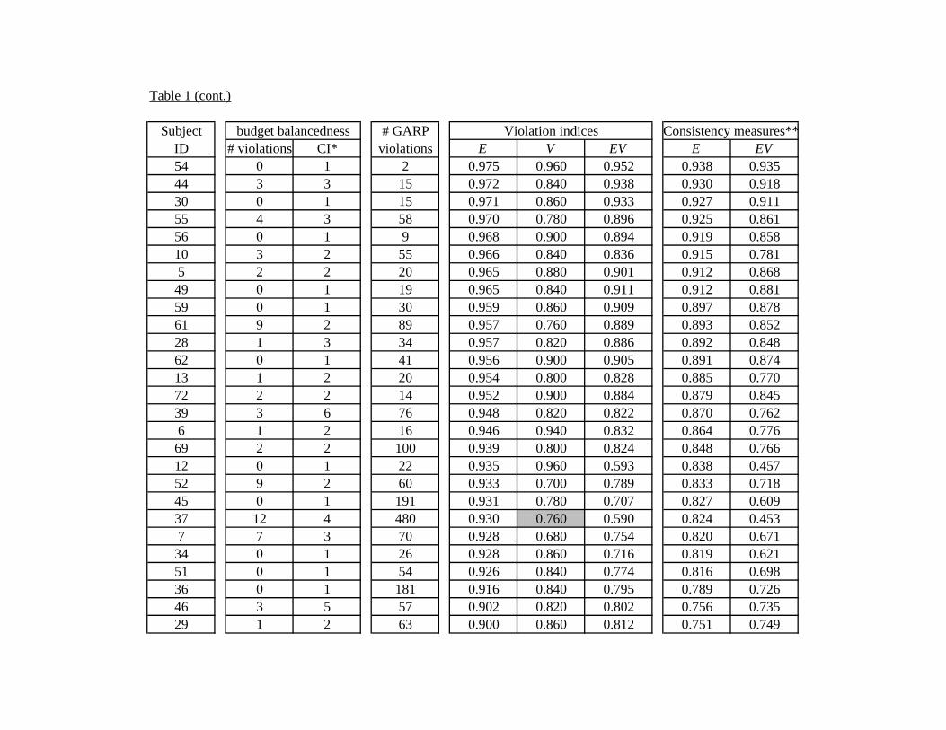
Table 1 (cont.)

Subject # GARPID # violations CI* violations E V EV E EV54 0 1 2 0.975 0.960 0.952 0.938 0.93544 3 3 15 0.972 0.840 0.938 0.930 0.91830 0 1 15 0.971 0.860 0.933 0.927 0.91155 4 3 58 0.970 0.780 0.896 0.925 0.86156 0 1 9 0.968 0.900 0.894 0.919 0.85810 3 2 55 0.966 0.840 0.836 0.915 0.7815 2 2 20 0.965 0.880 0.901 0.912 0.868

49 0 1 19 0.965 0.840 0.911 0.912 0.88159 0 1 30 0.959 0.860 0.909 0.897 0.87861 9 2 89 0.957 0.760 0.889 0.893 0.85228 1 3 34 0.957 0.820 0.886 0.892 0.84862 0 1 41 0.956 0.900 0.905 0.891 0.87413 1 2 20 0.954 0.800 0.828 0.885 0.77072 2 2 14 0.952 0.900 0.884 0.879 0.84539 3 6 76 0.948 0.820 0.822 0.870 0.7626 1 2 16 0.946 0.940 0.832 0.864 0.776

69 2 2 100 0.939 0.800 0.824 0.848 0.76612 0 1 22 0.935 0.960 0.593 0.838 0.45752 9 2 60 0.933 0.700 0.789 0.833 0.71845 0 1 191 0.931 0.780 0.707 0.827 0.60937 12 4 480 0.930 0.760 0.590 0.824 0.4537 7 3 70 0.928 0.680 0.754 0.820 0.671

34 0 1 26 0.928 0.860 0.716 0.819 0.62151 0 1 54 0.926 0.840 0.774 0.816 0.69836 0 1 181 0.916 0.840 0.795 0.789 0.72646 3 5 57 0.902 0.820 0.802 0.756 0.73529 1 2 63 0.900 0.860 0.812 0.751 0.749

budget balancedness Violation indices Consistency measures**

Table 1 (cont.)

Subject # GARPID # violations CI* violations E V EV E EV73 3 5 221 0.899 0.680 0.676 0.748 0.56770 0 1 24 0.892 0.840 0.877 0.731 0.83566 2 2 541 0.865 0.800 0.518 0.663 0.35664 6 5 132 0.848 0.720 0.693 0.619 0.59021 0 1 539 0.845 0.820 0.486 0.612 0.3131 0 1 376 0.844 0.780 0.464 0.610 0.284

11 1 2 209 0.834 0.840 0.658 0.586 0.5433 4 6 332 0.817 0.700 0.390 0.544 0.185

43 0 1 248 0.811 0.740 0.510 0.529 0.34614 5 2 19 0.806 0.840 0.741 0.514 0.65447 17 12 359 0.798 0.600 0.533 0.494 0.37775 26 6 446 0.792 0.760 0.540 0.479 0.38663 1 2 73 0.716 0.940 0.507 0.290 0.34219 15 9 497 0.710 0.660 0.256 0.276 0.00674 21 15 521 0.697 0.800 0.402 0.242 0.20253 2 4 942 0.619 0.840 0.196 0.048 -0.07416 42 15 1005 0.606 0.840 0.205 0.016 -0.06271 31 23 528 0.582 0.760 0.364 -0.046 0.1512 8 12 1089 0.517 0.840 0.244 -0.207 -0.010

48 6 20 1037 0.500 0.860 0.069 -0.251 -0.24326 10 32 797 0.272 0.840 0.185 -0.821 -0.08876 49 41 1216 0.211 0.860 0.066 -0.973 -0.248

***

Lower bounds.index of one and the average random-choice index.The difference between the actual index and the average random-choice index as a fraction of the difference between The confidence interval required to remove all budget balancedness violations.

budget balancedness Violation indices Consistency measures**

ID ρ α σ A r A r F -value73 -14.813 1.000 -0.063 9.980 0.937 0.708 0.055 -87.79446 -5.369 0.658 -0.157 1.108 0.843 0.031 0.040 -86.60855 -2.786 0.993 -0.264 3.678 0.736 0.178 0.057 -79.2273 -2.324 0.679 -0.301 1.253 0.699 0.089 0.085 -39.73643 -0.672 0.961 -0.598 6.814 0.402 1.120 0.134 -39.69036 -0.511 0.866 -0.662 3.430 0.338 0.270 0.067 -52.57718 -0.507 0.554 -0.664 1.153 0.336 0.043 0.036 -69.36837 -0.489 0.685 -0.672 1.686 0.328 0.099 0.071 -48.82110 -0.476 0.971 -0.678 10.749 0.322 0.974 0.066 -86.6211 -0.439 0.827 -0.695 2.970 0.305 0.332 0.150 -27.70564 -0.435 0.962 -0.697 9.446 0.303 1.965 0.182 -23.83145 -0.326 0.940 -0.754 7.924 0.246 1.046 0.133 -53.67313 -0.132 0.922 -0.883 8.912 0.117 0.792 0.092 -75.70761 -0.115 0.959 -0.897 16.978 0.103 1.654 0.126 -98.71170 -0.111 0.864 -0.900 5.277 0.100 0.448 0.104 -58.06421 -0.097 0.669 -0.912 1.897 0.088 0.167 0.100 -27.19756 -0.083 0.517 -0.924 1.065 0.076 0.045 0.043 -60.1286 -0.060 0.503 -0.943 1.012 0.057 0.020 0.020 -99.71532 -0.040 0.516 -0.962 1.064 0.038 0.012 0.010 -128.90040 -0.011 0.505 -0.989 1.020 0.011 0.014 0.012 -115.90049 0.027 0.530 -1.028 1.133 -0.028 0.061 0.059 -53.31752 0.114 0.767 -1.129 3.834 -0.129 0.281 0.059 -57.055

Standard errors

Table 2. Results of individual-level CES demand function estimation

Table 2 (cont.)

ID ρ α σ A r A r F -value11 0.144 0.927 -1.168 19.575 -0.168 6.190 0.290 -36.33072 0.170 0.670 -1.205 2.349 -0.205 0.155 0.073 -48.24138 0.219 0.787 -1.280 5.323 -0.280 0.430 0.084 -61.86669 0.231 0.638 -1.300 2.092 -0.300 0.197 0.108 -28.39329 0.260 0.922 -1.351 28.095 -0.351 17.856 0.443 -20.95734 0.291 0.532 -1.410 1.200 -0.410 0.099 0.077 -30.19728 0.315 0.893 -1.460 22.187 -0.460 9.393 0.278 -16.37566 0.329 0.581 -1.490 1.631 -0.490 0.181 0.123 -18.56215 0.334 0.699 -1.501 3.549 -0.501 0.183 0.057 -72.85550 0.337 0.579 -1.509 1.614 -0.509 0.084 0.064 -55.39630 0.428 0.657 -1.747 3.123 -0.747 0.287 0.096 -46.6779 0.493 0.748 -1.972 8.575 -0.972 0.905 0.110 -60.64923 0.497 0.746 -1.987 8.508 -0.987 1.295 0.129 -32.9817 0.543 0.706 -2.187 6.775 -1.187 1.193 0.167 -43.89141 0.577 0.812 -2.362 31.464 -1.362 8.512 0.151 -75.66439 0.583 0.649 -2.399 4.393 -1.399 0.709 0.152 -30.94414 0.615 0.771 -2.598 23.339 -1.598 8.231 0.204 -38.7805 0.658 0.576 -2.923 2.463 -1.923 0.293 0.230 -31.05659 0.674 0.522 -3.065 1.317 -2.065 0.146 0.235 -31.64051 0.702 0.580 -3.351 2.970 -2.351 0.766 0.373 1.95712 0.823 0.639 -5.659 25.376 -4.659 25.809 1.452 26.9958 0.942 0.532 -17.346 9.204 -16.346 5.941 3.734 -13.03754 0.992 0.504 -117.970 6.345 -116.970 12.567 36.202 -96.376

Standard errors

Figure 1A. Decision-level distribution of expenditure on tokens given to othersas a fraction of total expenditure on tokens

0.00

0.05

0.10

0.15

0.20

0.25

0.30

0.35

0.40

0.45

0.50

0.55

0.60

0-0.05 0.05-0.15

0.15-0.25

0.25-0.35

0.35-0.45

0.45-0.55

0.55-0.65

0.65-0.75

0.75-0.85

0.85-0.95

0.95-1

Flat slopes Intermediate slopes Steep slopes All

Figure 1B. Decision-level distribution of tokens given to others as a fraction of total tokens kept and given

0.00

0.05

0.10

0.15

0.20

0.25

0.30

0.35

0.40

0.45

0.50

0.55

0.60

0-0.05 0.05-0.15

0.15-0.25

0.25-0.35

0.35-0.45

0.45-0.55

0.55-0.65

0.65-0.75

0.75-0.85

0.85-0.95

0.95-1

Flat slopes Intermediate slopes Steep slopes All

Figure 2. The distribution of the expenditure on tokens given to others a fraction of total expenditureaggregated to the subject level

0.00

0.05

0.10

0.15

0.20

0.25

0.30

0-0.05 0.05-0.15

0.15-0.25

0.25-0.35

0.35-0.45

0.45-0.55

0.55-0.65

0.65-0.75

0.75-0.85

0.85-0.95

0.95-1

Frac

tion

of su

bjec

ts

Figure 3. The allocations of subjects with prototypical references

0

10

20

30

40

50

60

70

80

90

100

0 10 20 30 40 50 60 70 80 90 100

Selfish (ID 4)

0

10

20

30

40

50

60

70

80

90

100

0 10 20 30 40 50 60 70 80 90 100

Utilitarian (ID 54)

Self Self

OtherOther

0

10

20

30

40

50

60

70

80

90

100

0 10 20 30 40 50 60 70 80 90 100

Rawlsian (ID 46)

Other

Self

Figure 4. The construction of the E -index for a simple violation of GARP

AB

C

D

π

π'

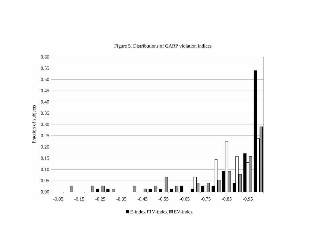
Figure 5. Distributions of GARP violation indices

0.00

0.05

0.10

0.15

0.20

0.25

0.30

0.35

0.40

0.45

0.50

0.55

0.60

-0.05 -0.15 -0.25 -0.35 -0.45 -0.55 -0.65 -0.75 -0.85 -0.95

Frac

tion

of su

bjec

ts

E-index V-index EV-index

Figure 6. Distribution of (normalized) consistency values

0.00

0.05

0.10

0.15

0.20

0.25

0.30

0.35

0.40

0.45

0.50

0.55

0.60

-0 0-0.1 0.1-0.2 0.2-0.3 0.3-0.4 0.4-0.5 0.5-0.6 0.6-0.7 0.7-0.8 0.8-0.9 0.9-1

Frac

tion

of su

bjec

ts

E-index EV-index

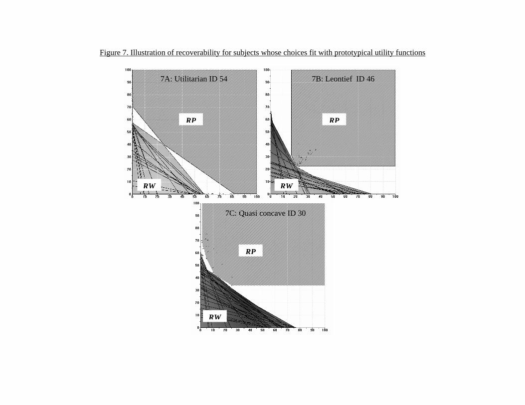
Figure 7. Illustration of recoverability for subjects whose choices fit with prototypical utility functions

RW RW

RW

RP

RP RP

7A: Utilitarian ID 54 7B: Leontief ID 46

7C: Quasi concave ID 30

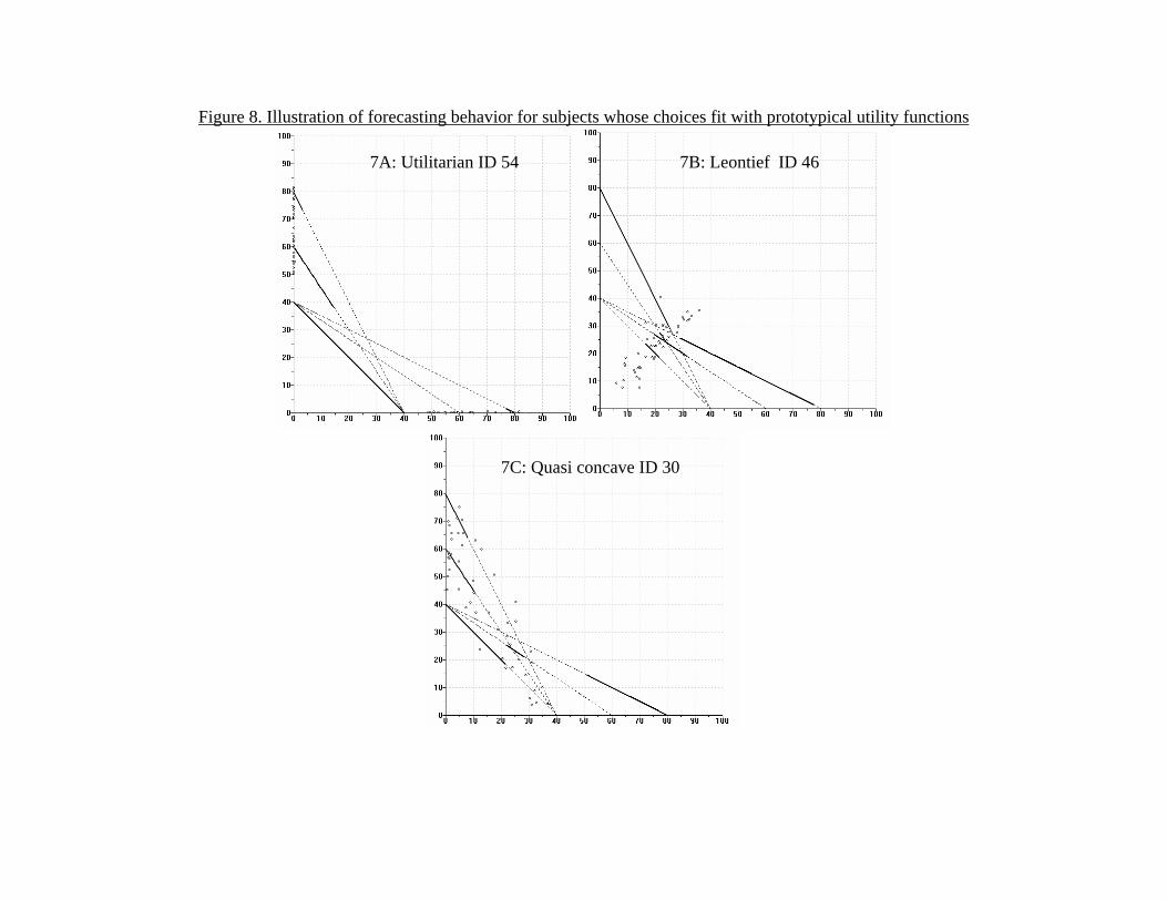
Figure 8. Illustration of forecasting behavior for subjects whose choices fit with prototypical utility functions

7A: Utilitarian ID 54 7B: Leontief ID 46

7C: Quasi concave ID 30

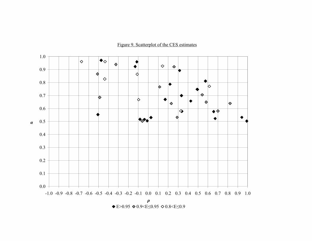
Figure 9. Scatterplot of the CES estimates

0.0

0.1

0.2

0.3

0.4

0.5

0.6

0.7

0.8

0.9

1.0

-1.0 -0.9 -0.8 -0.7 -0.6 -0.5 -0.4 -0.3 -0.2 -0.1 0.0 0.1 0.2 0.3 0.4 0.5 0.6 0.7 0.8 0.9 1.0

E>0.95 0.9<E≤0.95 0.8<E≤0.9ρ

α

Figure 10. The distribution of the CES parameter(rounded to a single decimal place)

0.00

0.02

0.04

0.06

0.08

0.10

0.12

0.14

0.16

0.18

0.20

-1 -0.9 -0.8 -0.7 -0.6 -0.5 -0.4 -0.3 -0.2 -0.1 0 0.1 0.2 0.3 0.4 0.5 0.6 0.7 0.8 0.9 1

E≥0.95 E≥0.90 E≥0.80ρ

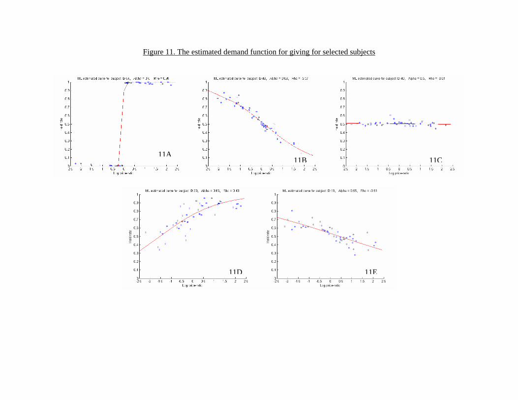
Figure 11. The estimated demand function for giving for selected subjects

11A11B 11C

11D 11E

Figure 12. The estimated indirect utility function for selected subjects

12A 12B 12C

12D 12E

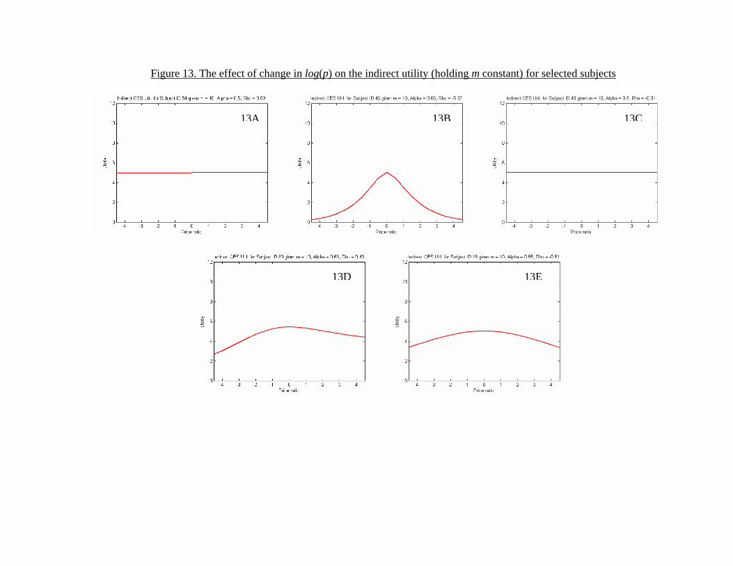
Figure 13. The effect of change in log(p) on the indirect utility (holding m constant) for selected subjects

13A 13B 13C

13D 13E

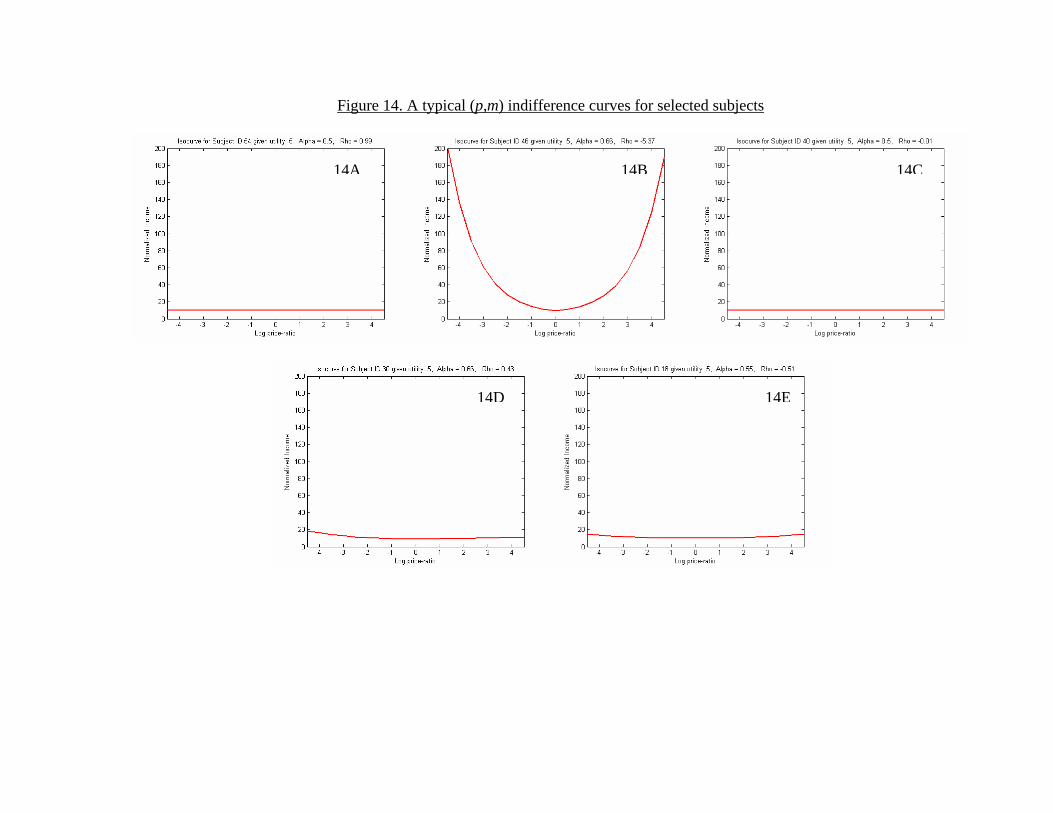
Figure 14. A typical (p,m) indifference curves for selected subjects

14A 14B 14C

14D 14E

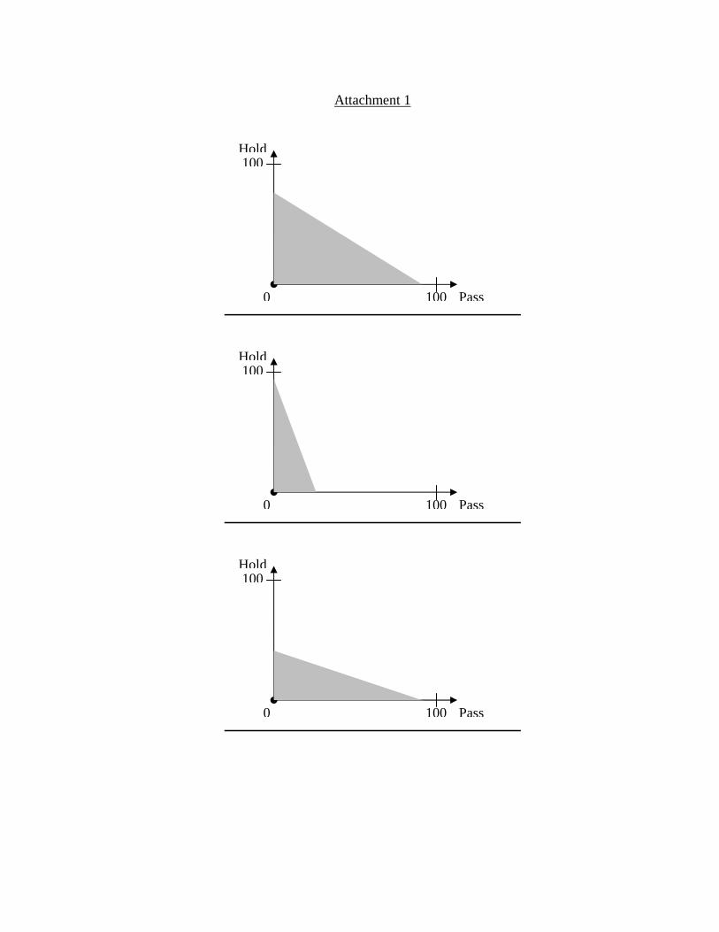
Attachment 1

Hold

Pass0 100

100

Hold

Pass0 100

100

Hold

Pass0 100

100

Attachment 2

Hold

Pass0 100

100

B

z

w

Hold

Pass0 100

100

Ay

x