
Neural coding of a natural stimulus ensemble: Uncovering ...

Individual and Ensemble Functional Link
Neural Networks for Data Classification
by
Toktam Babaei
BSc. and MSc Physics
Submitted in fulfilment of the requirements for the degree of
Doctor of Philosophy
Deakin University
December, 2017


iii
Abstract
In artificial neural network (ANN) research, the functional link neural network (FLNN) is a
well-known alternative to the standard feedforward ANNs such as the Multilayer Perceptron
network. The FLNN has a flat structure, i.e., with no hidden layer(s), therefore reducing its
structure complexity while retaining the capability of solving non-linear classification and
regression problems. This research focuses on using different FLNN-based models to tackle
data classification tasks. Firstly, an evolutionary-based modification to the FLNN, known as
reduced-FLNN1 (rFLNN1), is proposed to optimise the network structure and improve its
classification performance. Encouraged by the good performance of rFLNN1, another
improved version, known as reduced-FLNN2 (rFLNN2), is proposed. The rFLNN2 model
merges optimisation of both network structure and network weights into one search problem,
in order to generate a parsimonious FLNN model with high classification capabilities. To
further improve the robustness of rFLNN2 an ensemble of multiple rFLNN2-based models is
formulated. Coupled with the behavioural knowledge space and a novel decision fusion
method based on the ordered weighted averaging operator, the ensemble model is able to
handle noise-corrupted data classification problems. Extensive experiments covering
benchmark classification problems from the machine learning repository of the University of
California, Irvine and KEEL-data set repository are performed to evaluate the effectiveness of
the proposed rFLNN-based individual and ensemble models for data classification. In addition
to benchmark data sets, two real-world problems are used for evaluation. The results are
analysed, discussed, and compared with those published in the literature. The outcomes
positively demonstrate the potential and efficacy of the proposed rFLNN-based models for
undertaking data classification problems.

iv
List of Publications
T. Babaei, H. Abdi, C. P. Lim, and S. Nahavandi, "A study and a directory of energy
consumption data sets of buildings," Energy and Buildings, vol. 94, 2015, pp. 91-99
T. Babaei, C. P. Lim, H. Abdi, and S. Nahavandi, "A Modified Functional Link Neural
Network for Data Classification," in Emerging Trends in Neuro Engineering and Neural
Computation, ed: Springer, 2017, pp. 229-244
I. Hettiarachchi, T.Babaei, T. Thi Nguyen, C.P. Lim, S. Nahavandi, "A fresh look at
functional link neural network for motor imagery-based brain-computer interface" , J. of
Neuroscience Methods, (Accepted with minor revisions)

v
Acknowledgment
I am sincerely grateful to my advisors Saeid Nahavandi, Chee Peng Lim, and Hamid Abdi,
who are brilliant researchers and amazing persons. I am deeply thankful to my principal
supervisor Saeid Nahavandi for his continues supports and encouragements. I would also like
to express my deepest gratitude to my co-supervisor Chee Peng Lim, who will always remain
a source of inspiration to me. His enthusiasm along with the knowledge and patience with
which he approaches problems and builds insights make him an ideal advisor to have. I would
also like to thank my other co-supervisor Hamid Abdi for his supports and for sharing his
knowledge with me.
I am grateful to my family and friends for being a constant source of encouragement and
motivation. Most of all, I would like to thank my parents for fostering in me the love of learning
and discovery and encouraging me to follow my heart.

vi
Contents
Abstract .................................................................................................................................... iii
List of Publications ................................................................................................................... iv
Acknowledgment ....................................................................................................................... v
List of Figures: .......................................................................................................................... ix
List of Tables ............................................................................................................................ xi
List of Abbreviations ............................................................................................................. xiii
Introduction ........................................................................................................................ 1
1.1 Artificial Intelligence .................................................................................................. 1
1.2 Data classification and Artificial Neural Networks .................................................... 2
1.3 Problem statement and motivations ............................................................................ 3
1.4 Research aim and objectives ....................................................................................... 4
1.5 Research methodology ................................................................................................ 5
1.6 Outline of the thesis..................................................................................................... 6
Background and Literature Review .................................................................................... 8
2.1 Overview of Artificial Neural Networks ..................................................................... 8
2.2 Functional Link Neural Network (FLNN) ................................................................ 12
Computational Complexity ................................................................................ 14
On-Line Learning............................................................................................... 15
2.3.2 Related Studies on the FLNN ............................................................................ 16
2.4 Evolution of Neural Networks .................................................................................. 20
2.5 Evolutionary Feature selection .................................................................................. 23
2.6 Remarks on Evolutionary methods ........................................................................... 27
2.7 Ensemble Methods .................................................................................................... 27
2.7.1 Related Studies on Ensemble Methods .............................................................. 30
2.8 Remarks on Ensemble Methods ................................................................................ 33
2.9 Chapter Summary ...................................................................................................... 35
Research Methodology ..................................................................................................... 37
3.1 Functional link neural networks with different basis functions ................................ 38
Power polynomials of p-FLNN ......................................................................... 40

vii
Trigonometric functions of tr-FLNN ................................................................. 41
Legendre polynomials of Le-FLNN .................................................................. 41
Chebyshev polynomials ..................................................................................... 41
3.2 The Proposed rFLNN1 Model................................................................................... 42
3.3 The Proposed rFLNN2 Model................................................................................... 46
3.4 An Ensemble of rFLNN2-based Models ................................................................... 50
3.4.1 The BKS Combination Method ......................................................................... 51
3.4.2 The Ordered Weighted Averaging Aggregation Operator ................................. 53
3.5 Chapter Summary ...................................................................................................... 60
Experimental Results, Analysis, and Discussion .............................................................. 62
4.1 Description of Benchmark Data Sets ........................................................................ 63
4.2 Noisy data .................................................................................................................. 69
4.3 Performance Metrics ................................................................................................. 70
4.4 Comparison of Two Classifiers ................................................................................. 71
4.5 FLNNs with different basis functions ....................................................................... 72
Results and discussion for FLNNs experiments ................................................ 73
Remarks on FLNNs with different basis functions ............................................ 80
4.6 rFLNN Models .......................................................................................................... 80
Experimental Procedure for rFLNN1 ................................................................ 81
rFLNN1 Configurations ..................................................................................... 82
Results of the rFLNN1 Evaluation .................................................................... 82
Remarks on rFLNN1 model............................................................................... 86
Experimental Procedure for rFLNN2 ................................................................ 86
Results of the rFLNN2 Evaluation .................................................................... 86
4.7 Ensemble rFLNN2 Model ......................................................................................... 87
Experimental Procedure for the rFLNN2 Ensemble Model .............................. 88
Results and Discussion of the rFLNN2 Ensemble Model ................................. 88
Evaluation of rFLNN2 Ensemble Model with BKS-OWA and BKS-SB systems
91
Results and Discussion of rFLNN2 Ensemble with BKS-OWA and BKS-SB
systems 93
Evaluation of rFLNN2 Ensemble Model ........................................................... 94
4.8 Real-World Classification Problems ......................................................................... 98
Power Quality Monitoring ................................................................................. 98
Motor Fault diagnosis ........................................................................................ 99

viii
4.9 Chapter Summary .................................................................................................... 101
Conclusions and Future Research ................................................................................... 103
5.1 Conclusions ............................................................................................................. 103
5.2 Suggestions for Further Research ........................................................................... 104
References .............................................................................................................................. 106

ix
List of Figures:
Figure 1.1: Summary of the relationship of research methodology........................................... 5
Figure 1.2: Overview of research methodology ........................................................................ 7
Figure 2.1: Schematic representation of a real neuron .............................................................. 9
Figure 2.2: Representation of an artificial neuron-single perceptron, w0 indicates the
threshhold value of the perceptron ............................................................................................. 9
Figure 2.4: A schematic diagram of an MLP with two hidden layers, with h1 neurons in the
first hidden layer and h2 neurons in the second hidden layer .................................................. 10
Figure 2.5: The backpropagation algorithm for training the MLP network ............................ 11
Figure 2.6: Schematic diagram of FLNN ................................................................................ 13
Figure 2.7: Pseudo code for standard GA algorithm ............................................................... 26
Figure 2.8: Schematic representation of an ensemble classification system. Decisions from
individual classifiers are combined to generate the final decision .......................................... 29
Figure 3.1: Structure of FLNN models with different basis functions used in this work ........ 39
Figure 3.2: Pseudo code for FLNN .......................................................................................... 40
Figure 3.3: Data representation of circle-square classification problem (left), same problem in
{𝑥12, 𝑥2
2} space (right)............................................................................................................ 44
Figure 3.4 : A chromosome and corresponding network in rFLNN1 ...................................... 44
Figure 3.5:Algorithm description of rFLNN1 ......................................................................... 45
Figure 3.6: Topology of the rFLNN1 model ........................................................................... 46
Figure 3.7:Topological structure of rFLNN2........................................................................... 47
Figure 3.8: A chromosome and corresponding network in rFLNN2 ....................................... 48
Figure 3.9: Cross over in rFLNN2 and the two resulted children ........................................... 49
Figure 3.10:The first scenario of mutation in rFLNN2 system; the mutation point was
selected from the binary part .................................................................................................... 49
Figure 3.11: Overview of ensemble classification system with rFLNN2 individual classifiers
and BKS combination method ................................................................................................. 50
Figure 3.12: Quantifier functions "all"(𝑄∗(𝑟)) and "any" (𝑄∗(𝑟)) .......................................... 55
Figure 3.13: Exploiting weights from a quantifier function .................................................... 55
Figure 3.14: Steps to make final decision using the support value of an alternative given by m
agents, using the OWA aggregation operator, where OWA weights are calculated using the
quantifier function, Q. .............................................................................................................. 57
Figure 3.15: Algorithm representation of ensemble rFLNN2 model ...................................... 59

x
Figure 3.16: Schematic diagram of operation phase in BKS-OWA ensemble model.𝜑_3
indicates the degrees of membership to each class (Section 2-7) ............................................ 60
Figure 4.1: Schema of k-fold cross validation ......................................................................... 71
Figure 4.2: Test accuracies of FLNNs with 4 different basis functions on 12 benchmark data
sets............................................................................................................................................ 75
Figure 4.3: Average of average accuracies with different noise placements in train and test
sets respectively ....................................................................................................................... 79
Figure 4.4: True class labels and class predictions by Poly-,Tr-,Le-,and Ch- FLNN classifiers
for 67 test samples of Ecoli problem in a fold ........................................................................ 80
Figure 4.5: Schematic diagram of HFLNN proposed in [32] vs. rFLNN1 with the same basis
functions ................................................................................................................................... 81
Figure 4.6: Performance comparison (bottom) with respect to maximum training accuracy
(top) .......................................................................................................................................... 84
Figure 4.7: Fraction of discarded expanded features ............................................................... 85
Figure 4.8: Percentage of weights in rFLNN2 and EFLNN models compared to that in
original FLNN .......................................................................................................................... 88
Figure 4.9: 5-fold classification accuracy results for clean train –noisy test datasets ............. 92
Figure 4.10: 5-fold rejection rate results for data sets with different clean and noisy
configurations. ......................................................................................................................... 92
Figure 4.11: Schematic diagram of fault detection and diagnosis (adapted from [182]) ...... 100
xi
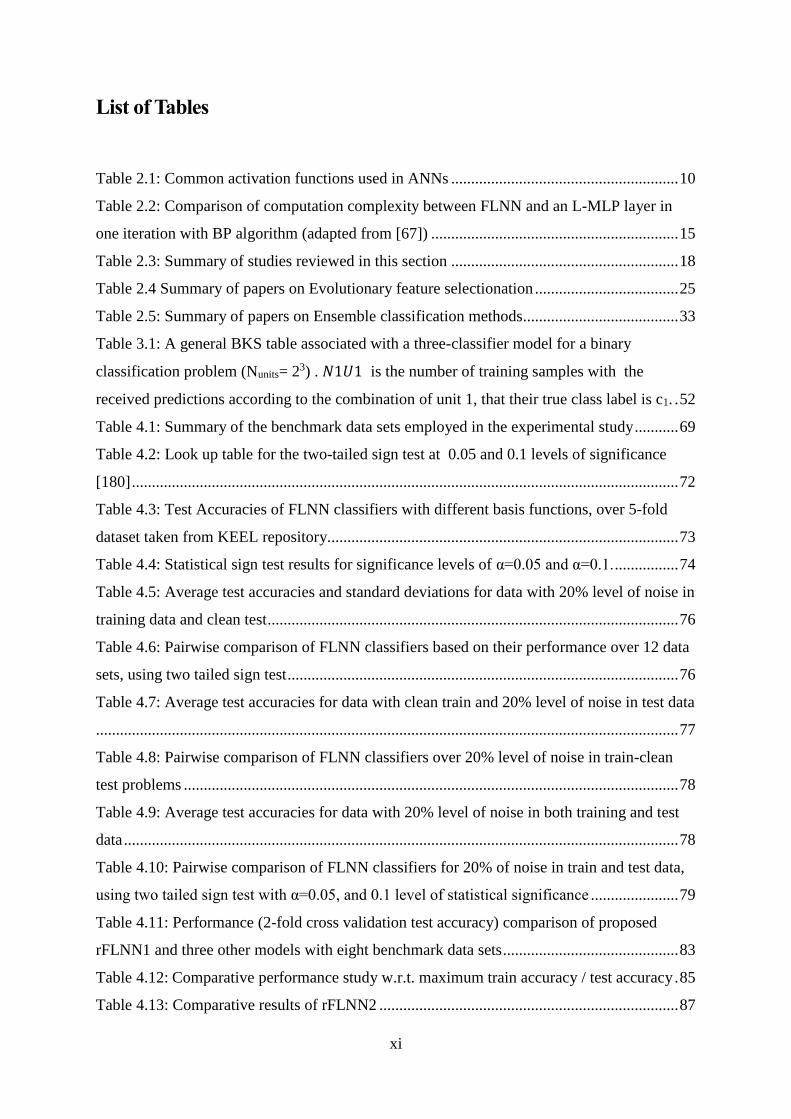
List of Tables
Table 2.1: Common activation functions used in ANNs ......................................................... 10
Table 2.2: Comparison of computation complexity between FLNN and an L-MLP layer in
one iteration with BP algorithm (adapted from [67]) .............................................................. 15
Table 2.3: Summary of studies reviewed in this section ......................................................... 18
Table 2.4 Summary of papers on Evolutionary feature selectionation .................................... 25
Table 2.5: Summary of papers on Ensemble classification methods....................................... 33
Table 3.1: A general BKS table associated with a three-classifier model for a binary
classification problem (Nunits= 23) . 𝑁1𝑈1 is the number of training samples with the
received predictions according to the combination of unit 1, that their true class label is c1. . 52
Table 4.1: Summary of the benchmark data sets employed in the experimental study ........... 69
Table 4.2: Look up table for the two-tailed sign test at 0.05 and 0.1 levels of significance
[180] ......................................................................................................................................... 72
Table 4.3: Test Accuracies of FLNN classifiers with different basis functions, over 5-fold
dataset taken from KEEL repository........................................................................................ 73
Table 4.4: Statistical sign test results for significance levels of α=0.05 and α=0.1. ................ 74
Table 4.5: Average test accuracies and standard deviations for data with 20% level of noise in
training data and clean test ....................................................................................................... 76
Table 4.6: Pairwise comparison of FLNN classifiers based on their performance over 12 data
sets, using two tailed sign test .................................................................................................. 76
Table 4.7: Average test accuracies for data with clean train and 20% level of noise in test data
.................................................................................................................................................. 77
Table 4.8: Pairwise comparison of FLNN classifiers over 20% level of noise in train-clean
test problems ............................................................................................................................ 78
Table 4.9: Average test accuracies for data with 20% level of noise in both training and test
data ........................................................................................................................................... 78
Table 4.10: Pairwise comparison of FLNN classifiers for 20% of noise in train and test data,
using two tailed sign test with α=0.05, and 0.1 level of statistical significance ...................... 79
Table 4.11: Performance (2-fold cross validation test accuracy) comparison of proposed
rFLNN1 and three other models with eight benchmark data sets ............................................ 83
Table 4.12: Comparative performance study w.r.t. maximum train accuracy / test accuracy . 85
Table 4.13: Comparative results of rFLNN2 ........................................................................... 87

xii
Table 4.14: Five folds cross validation accuracy of rFLNN2 ensemble with normal BKS and
with BKS-OWA combination systems - results for clean datasets five folds ......................... 89
Table 4.15: Five folds cross validation accuracy of rFLNN2 ensemble with normal BKS and
with BKS-OWA combination systems- results for noisy train –clean test datasets ............. 89
Table 4.16: Five folds cross validation accuracy of rFLNN2 ensemble with normal BKS and
with BKS-OWA combination systems- results for clean train –noisy test datasets ............... 90
Table 4.17: Five folds cross validation accuracy of rFLNN2 ensemble with standard BKS and
with BKS-OWA combination systems for noisy train-noisy test datasets .............................. 90
Table 4.18: Test accuracy of rFLNN2 ensemble with BKS-SB BKS- OWA systems. The
higher performance for each problem is bolded. ..................................................................... 93
Table 4.19: Comparison of classification accuracies obtained for proposed ensemble model
with eight other Ensemble classifiers ...................................................................................... 97
Table 4.20: Pairwise comparison of rFLNN2 ensemble with BKS-OWA system. The
rFLNN2 ensemble with BKS-OWA is α- level significantly better than other system
considering the cases it performed better on the 12 cases ....................................................... 98
Table 4.21: Summary of key characteristics of the Power quality dataset .............................. 99
Table 4.22: rFLNN2 ensemble with Standard BKS and with BKS-OWA combination
systems- results for power quality monitoring problem .......................................................... 99
Table 4.23: Summary of key characteristics of the induction motor fault diagnosis dataset 100
Table 4.24: rFLNN2 ensemble with normal BKS and BKS_OWA combination systems -
results for four motor faults diagnosis problem ..................................................................... 101

xiii
List of Abbreviations
AI Artificial Intelligence
ANN Artificial Neural Network
BKS Behavioural Knowledge Space
BP Back Propagation
DCS Dynamic Classifier Selection
DES Dynamic Ensemble Selection
EA Evolutionary Algorithm
FLNN Functional Link Neural Network
FNFN Functional Neural Fuzzy Network
GA Genetic Algorithm
HONN Higher Order Neural Network
HS Harmony Search
MA Memetic Algorithm
MCR Measure of Competence Based on Random classification
MCS Multiple Classifier Systems
MCSA Motor Current Signature Analysis
MFS Multiple Feature Subset
MLP Multi-Layer Perceptron
NMC Nearest Mean Classifier
NNE Neural Network Ensembles
OWA Ordered Weighted Averaging
rFLNN reduced Functional Link Neural Network
RVFLNN Random Vector Functional Link Neural Network

xiv
SLP Single Layer Perceptron
SVM Support Vector Machines
RVM Relevance Vector Machines
WAVE Weight-Adjusted Voting for Ensembles of classifiers

Introduction
This chapter starts with the preliminaries of artificial intelligence (AI) and artificial neural
networks (ANNs). It then presents the motivations for using the functional link neural network
(FLNN) for data classification, which is the main research focus of this thesis. A discussion on
the development of ensemble models for data classification is provided. The research
objectives and research methodology are explained. The thesis outline is described at the end
of this chapter.
1.1 Artificial Intelligence
The recognition of AI as an important research domain dates back to 1956[1]. The term
AI broadly refers to how a machine emulates the "cognitive" functions of the human brain, such
as "learning" and "problem solving", and uses them to operate autonomously in complex,
changing environments. In general, AI encompasses a number of machine learning
methodologies. They cover conventional statistics, neural computing, evolutionary computing,
and fuzzy computing models, to name a few [2]. The artificial neural network (ANN) is one of
key data-based learning AI methodologies.
In general, learning techniques can be divided into three categories: supervised learning,
unsupervised learning, and reinforcements learning [1]. Supervised learning establishes a
mapping function from a training set containing input-output data pairs. Regression and pattern
classification are supervised learning tasks, which comprise continuous and discrete outputs,
respectively. Data (pattern) classification is concerned with building machines to classify data
samples based on either a priori knowledge, or statistical information extracted from data
samples [3-5]. A classical definition of pattern is an entity that can be represented by a set of
attributes (a feature vector) [6]. As an example, a pattern can be an audio signal, where the
corresponding feature vector is its frequency spectral components; or a patient, where the feature
vector is the results of his/her medical tests. This thesis is focused on data classification
problems with supervised ANN models.

2
1.2 Data classification and Artificial Neural Networks
Data classification is a key task in accomplishing many activities. Accordingly, many studies
have been devoted to developing methods from different principles to solve data classification
problems. One of the earliest investigations is from the statistics community. Fisher [7] proposed a
linear discriminant function to tackle data classification problems. It was later extended to a
quadratic form[8]. Bayesian theory is another fundamental statistical method used in devising
various data classification methods [9, 10]. While these statistical principles have certain limitations
with respect to the underlying statistical assumptions [11, 12], they provided the necessary basis for
further research. In addition to statistical principles, a variety of AI-based models have been
researched for data classification, e.g. rough sets, fuzzy sets, decision trees, k-nearest neighbors, and
support vector machines (SVM).
Among different learning methodologies, ANNs are popular AI-based data learning models.
Indeed, research interest in ANNs stems from two aspects: (i) to understand and model
mathematically the biological nervous system in humans; (ii) to develop intelligent learning systems
that mimic the way how humans perform certain tasks, such as capturing data and interpreting
information. This research is concerned with the data learning aspect of ANNs, in view of the
potential impact of such learning models in undertaking data classification problems in the real
environments.
ANN emerges as useful data processing models [13]. To date, there are a number of
different ANN models, which include the Multi-Layer Perceptron (MLP) network [14] ,
Hopfield network [15, 16], and Radial Basis Function (RBF) network [16]. These models have
been used as a promising method to support and improve human decision-making in different
areas, e.g. function approximation [17-19], rule extraction [20], forecasting and prediction [21,
22], business [23, 24], engineering [25], and medicine [26]. An ANN requires knowledge
through a learning process. It simulates the inter-neuron connection strength as weights to
store knowledge [30]. As a result, it has unique characteristics including the ability to learn the
relationships between inputs and output data pairs for tackling data classification problems.
3
1.3 Problem statement and motivations
One of the popular ANN models is the Multilayer Perceptron (MLP). The input layer in
an MLP consists of units (neurons) equal in number to the input features and one bias unit. The
output layer consists of units equal in number to the output classes (labels). It has one or more
hidden layers in between the input and output layers. The role of the hidden units is to provide
the MLP with the capability of handling non-linear input-output mapping. It has been shown
that an MLP with a suitable architecture is able to approximate (or learn) any nonlinear decision
boundary [27]. Training the MLP includes finding the appropriate weights. The most common
training method is the back-propagation (BP) learning algorithm.
There are a number of issues in designing and developing an efficient and effective
learning algorithm for the MLP network, which include local minima, saturation, weight
interference, initial weight dependence, and overfitting. On the architecture side, the issues
include how to determine the number of hidden layers and the number of hidden units in an
MLP network. All these learning and architecture issues present great impacts on the usability
and usefulness of the MLP in tackling real-world problems. As such, a straight forward way
to avoid some of the key problems is to remove the hidden layer(s), which would compromise
the ability of an MLP to capture nonlinear input-output relationships. However, studies have
been shown that if higher order neurons (also known as sigma-pi neurons [28]) are added to
the original neurons in the input layer, an MLP network without any hidden layers could retain
its nonlinearity ability. This is the main idea behind the research on higher order neural
networks (HONNs) [29], [30]. HONNs have appeared as an attractive alternative to eradicating
some of the MLP limitations. In this respect, the functional link neural network (FLNN) poses
as a class of HONNs that utilizes a function of the original inputs to enhance the inputs [30].
In an FLNN, the hidden layers are removed and the network complexity is reduced, resulting
in a straightforward architecture and a straightforward learning process. These advantages
make FLNN attractive for researchers in the field [31-36], as the FLNN model alleviates the
key issue in determining the network complexity (the number of hidden nodes and hidden
layers) and the associated learning process of a standard MLP network, which is the building
block of deep learning models. In an FLNN, the number of enhanced inputs is determined by
the set of basis functions, and leaning can be framed in the form of a quadratic optimization
[37]. Moreover, a standard MLP network is not efficient in dealing with dynamically changing

4
environment which require an on-line learning capability. In this aspect, FLNN-based models
have been successfully used in undertakings on-line learning problems [37].
The design and development of FLNN-based learning models with the capability of
handling various data classification problems constitutes the main aim of this research. The
resulting models are evaluated using a variety of benchmark and real-world classification data
sets. On the other hand, studies have been shown that ensemble models, in which the
predictions from multiple classifiers are combined using a suitable decision combination
method, can generate more accurate decision for each input, therefore improving the overall
classification performance [38]. In this respect, majority voting is a straightforward strategy to
combine the decisions from an ensemble of individual classifiers. Other elaborated schemes
are also available to aggregate individual decisions, e.g. the behaviour knowledge space (BKS)
method. The BKS can efficiently aggregate decisions of individual classifiers to deliver better
results [39]. While the BKS can be used as an effective component in an ensemble model, it
has some limitations. The major limitation with the BKS is its rejection rate. When the BKS
fails to give a prediction for an input sample, due to lack of confidence, the input sample is
rejected [40-42]. This issue becomes serious when noisy data samples are available. Therefore,
this research investigates the use of an aggregation operator to tackle the rejection
problem of the BKS in an ensemble model.
1.4 Research aim and objectives
The main aim of this research is to formulate a framework that utilizes the FLNN-based
models as a useful and usable ensemble system for undertaking complex data classification
problems. The specific research objectives are as follows:
1. to enhance the FLNN by optimising its network architectures and overcoming issues
related to curse of dimensionality using evolutionary methods;
2. to improve the classification performance by devising an ensemble system consisting
of different individual FLNN-based models
3. to adapt an aggregation operator to effectively combine the predictions from multiple
individual FLNN-based models in the ensemble system
4. to apply the resulting individual and ensemble models to complex and noisy data
classification problems.
5
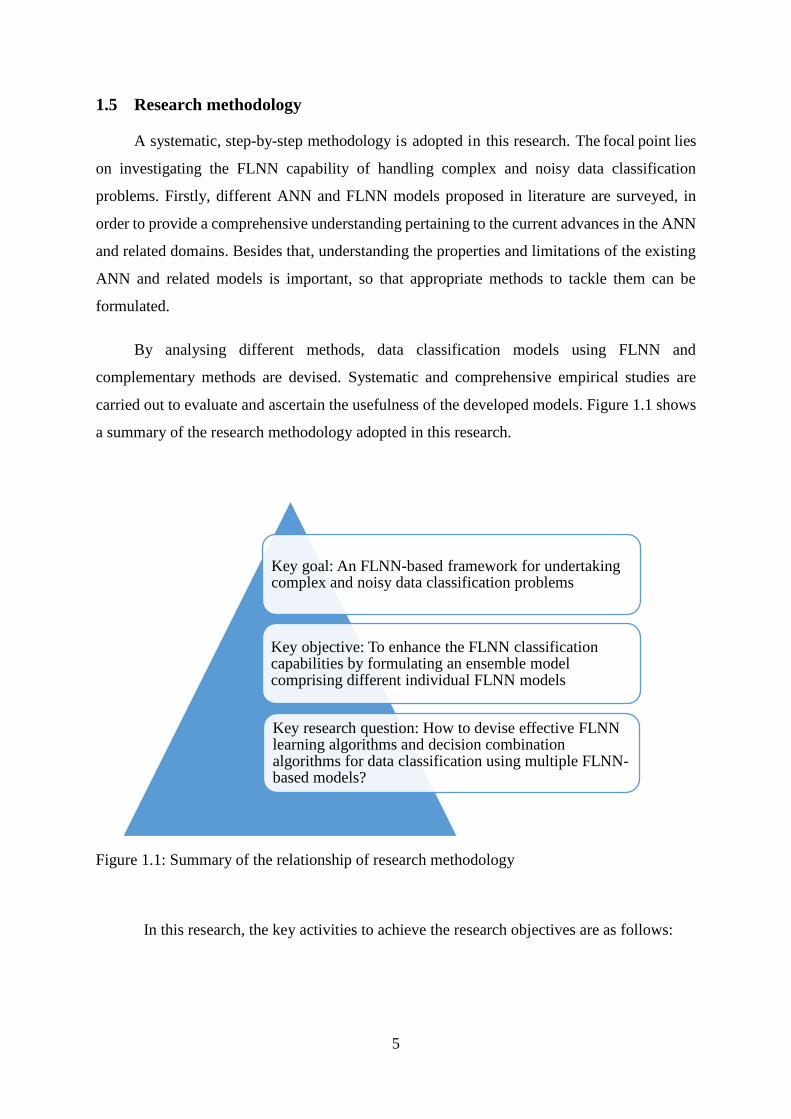
1.5 Research methodology
A systematic, step-by-step methodology is adopted in this research. The focal point lies
on investigating the FLNN capability of handling complex and noisy data classification
problems. Firstly, different ANN and FLNN models proposed in literature are surveyed, in
order to provide a comprehensive understanding pertaining to the current advances in the ANN
and related domains. Besides that, understanding the properties and limitations of the existing
ANN and related models is important, so that appropriate methods to tackle them can be
formulated.
By analysing different methods, data classification models using FLNN and
complementary methods are devised. Systematic and comprehensive empirical studies are
carried out to evaluate and ascertain the usefulness of the developed models. Figure 1.1 shows
a summary of the research methodology adopted in this research.
Figure 1.1: Summary of the relationship of research methodology
In this research, the key activities to achieve the research objectives are as follows:
Key goal: An FLNN-based framework for undertaking complex and noisy data classification problems
Key objective: To enhance the FLNN classification capabilities by formulating an ensemble model comprising different individual FLNN models
Key research question: How to devise effective FLNN learning algorithms and decision combination algorithms for data classification using multiple FLNN-based models?

6
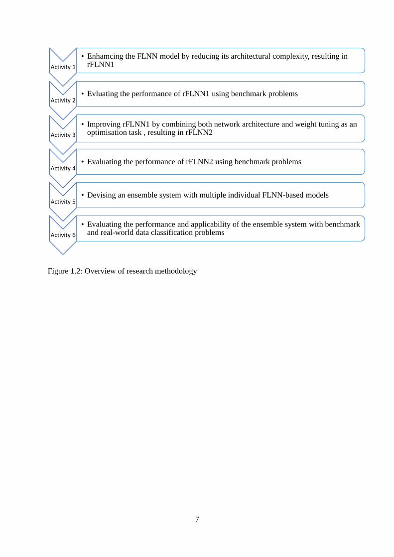
Activity 1. The FLNN classifier is thoroughly examined, in order to identify the existing
limitations, particularly the curse-of-dimensionality problem. This results in a parsimonious
FLNN model with reduced architectural complexity, known as rFLNN1.
Activity 2. The performance of rFLNN1 is evaluated comprehensively using benchmark data
sets, and the results are compared with those of other models reported in the literature.
Activity 3. An enhanced FLNN-based model using an evolutionary method, known as
rFLNN2, is proposed. Both network architecture and weight tuning are combined as
optimization problem, which is solved using the evolutionary method.
Activity 4. The performance of rFLNN2 is evaluated comprehensively using benchmark data
sets, and the results are compared with those of other models reported in the literature.
Activity 5. An ensemble system to tackle the problem of combining multiple predictions from
individual FLNN-based models with different expansion functions is formulated. An effective
aggregation operator is formulated for the ensemble system.
Activity 6. The performance of the ensemble model is comprehensively evaluated using
benchmark noisy data sets, and the results are compared with those of other models reported
in the literature. In addition, real-world data sets are used to ascertain the applicability of the
ensemble system in undertaking real data classification problems.
Figure 1.2 summarises the key activities of this research.
1.6 Outline of the thesis
The outline of the rest of this thesis is as follows. Chapter 2 contains the background
and literature review related to ANNs and FLNN-based models as well as complementary
methods such as evolutionary algorithms and ensemble methods. The detailed dynamics of the
proposed rFLNN models and the ensemble system are presented in Chapter 3. A
comprehensive experimental study with benchmark and real-world data sets is presented in
Chapter 4. The results are analysed, compared, and discussed thoroughly. Finally, conclusions
and suggestions for further research are presented in Chapter 5.
7
Figure 1.2: Overview of research methodology
Activity 1
• Enhamcing the FLNN model by reducing its architectural complexity, resulting in rFLNN1
Activity 2• Evluating the performance of rFLNN1 using benchmark problems
Activity 3
• Improving rFLNN1 by combining both network architecture and weight tuning as an optimisation task , resulting in rFLNN2
Activity 4• Evaluating the performance of rFLNN2 using benchmark problems
Activity 5• Devising an ensemble system with multiple individual FLNN-based models
Activity 6
• Evaluating the performance and applicability of the ensemble system with benchmark and real-world data classification problems

8
Background and Literature Review
As described in the first chapter, the focus of this thesis is on investigating the efficiency
of ANNs, particularly FLNN-based models, for data classification. The evolutionary
computing and ensemble methods are adopted. A linguistic aggregation operator, i.e., ordered
weighted average (OWA), is also used to combine multiple decisions in ensemble framework.
As such, this chapter provides the related background ANN, FLNN, evolutionary networks,
ensemble methods, and OWA operator as the linguistic aggregation operator is defined in this
framework. A critical review on the corresponding literature is also presented.
In the first section, the general standard MLP is described. Then the fundamental theory
of FLNN is presented. A review on the related publications in the literature is provided. The
review covers different FLNN variants and different applications. The next section deals with
evolutionary models, in which various evolutionary algorithms (EAs) to optimise ANNs are
reviewed. Then, a review on classification ensemble methods, with the focus on the ANN-
based ensemble models is presented.
2.1 Overview of Artificial Neural Networks
ANNs offer an important paradigm for approximating nonlinear decision boundaries in
classifying data. Being a black-box, they serve as valuable candidates when no appropriate
physical/mathematical models exist for complex data classification tasks. An ANN in general
consists of several processing units known as artificial neurons. These neurons are connected
together according to a topology to form a network that mimic the biological neurons of human
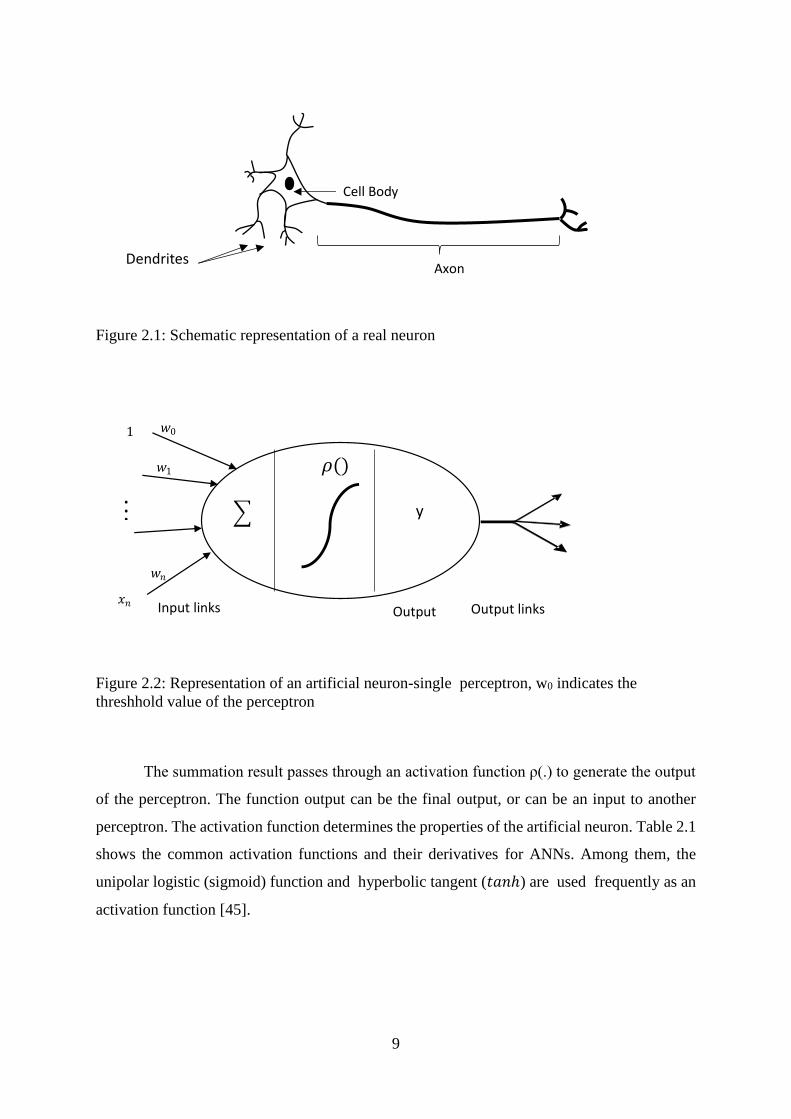
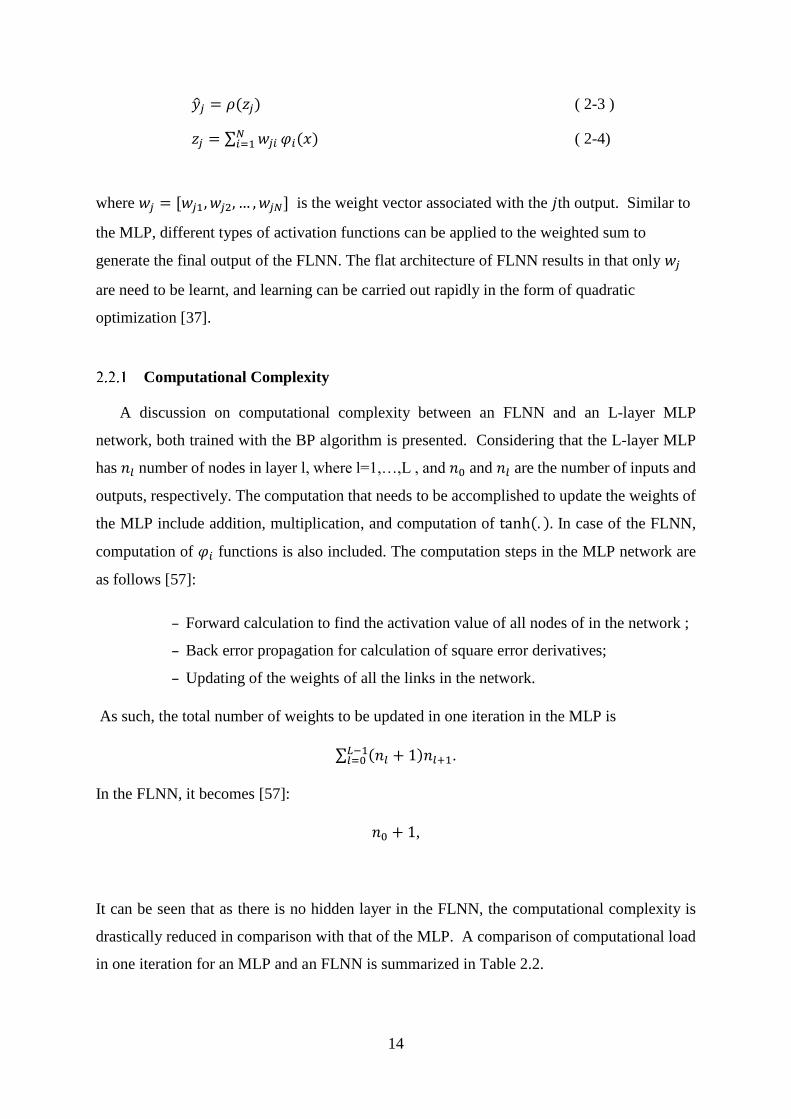
brain [43] . Figures 2.1 and 2.2 depict the biological neuron and its artificial counterpart. The
first mathematical model of an artificial neuron was proposed by McCulloch and Pitts in 1943
[13]. Then, Rosenblatt in 1957 [44] refined the artificial neuron, and devised the so-called
perceptron [45]. Equation (2-1) shows the mathematical model of an artificial neuron
𝑦 = 𝜌(∑ 𝑥𝑖𝑤𝑖𝑛𝑖=0 ) (2-1)
where the input features, {1, 𝑥1, 𝑥2, … , 𝑥𝑛}, are multiplied by the respective weight coefficients
𝑤0, 𝑤1, … , 𝑤𝑛, before the summation takes place.
9
Figure 2.1: Schematic representation of a real neuron
Figure 2.2: Representation of an artificial neuron-single perceptron, w0 indicates the
threshhold value of the perceptron
The summation result passes through an activation function ρ(.) to generate the output
of the perceptron. The function output can be the final output, or can be an input to another
perceptron. The activation function determines the properties of the artificial neuron. Table 2.1
shows the common activation functions and their derivatives for ANNs. Among them, the
unipolar logistic (sigmoid) function and hyperbolic tangent (𝑡𝑎𝑛ℎ) are used frequently as an
activation function [45].
Axon
Cell Body
Dendrites
Input links Output links Output
𝑤𝑛
𝜌()
𝑤0 1
𝑥𝑛
𝑤1
.
. . y

10
Table 2.1: Common activation functions used in ANNs
Name 𝝆(𝒛) = Derivative (𝝆′ =)
Logistic (Sigmoid) 1
1 + 𝑒−𝑧
𝜌(1 − 𝜌)
Hyperbolic tangent tanh (𝑧) (1 − 𝜌2)
Gaussian 𝑒−𝑧2 −2𝑧𝑒−𝑧2
Linear 𝑧 1
Binary threshold {0 𝑧 < 01 𝑧 ≥ 0
{0 𝑧 ≠ 0𝑈𝑛𝑑𝑒𝑓𝑖𝑛𝑒𝑑 𝑧 = 0
Soft plus ln (1 + 𝑒𝑧) 1
(1 + 𝑒−𝑧)
Figure 2.3 shows how a number of perceptron are organised in a network-like structure to
form the so-called Multi-Layer Perceptron (MLP). The key learning procedure of an MLP is
the back-propagation algorithm, which is summarised in Figure 2.4.
Figure 2.3: A schematic diagram of an MLP with two hidden layers, with h1 neurons in the
first hidden layer and h2 neurons in the second hidden layer
Inputs
Outputs
First hidden layer
Second hidden layer
.
.
𝑥2
𝑥𝑛
𝑦 1
𝑦 2
𝑥1
. . . .
𝑣1
𝑢ℎ1
𝑣ℎ2
𝑢1

11
Figure 2.4: The backpropagation algorithm for training the MLP network
Despite many successful applications of the MLP in function approximation and
classification tasks, one of the problems is the plateaus error surface of the MLP [46, 47]. This
is because gradient decent, as well as other training methods which are based on standard
numerical optimization techniques, is susceptible to local minima of the error surface. The local
minima trap poses a severe obstacle when the MLP is used to approximate complex functions.
In approximating complex functions, the MLP architecture could grow to thousands of
neurons, which makes the training process a difficult one.
function Backpropagation (𝑠𝑎𝑚𝑝𝑙𝑒𝑠, 𝑛𝑒𝑡𝑤𝑜𝑟𝑘 ) returns a neural network
inputs: (input vector x ,true output vector y) samples,
network , a multilayer network with L layers, weights 𝑤𝑖,𝑗, activation function
ρ
local variables: Δ, a vector of errors, indexed by network node
while (some stopping criterion satisfied) do
for each weight 𝑤𝑖,𝑗in the network
𝑤𝑖,𝑗 ←initialize randomly
for each sample (𝒙, 𝒚)
Propagate the inputs forward to compute the outputs
for each node 𝑖 in the input layer
𝑎𝑖←𝑥𝑖
for 𝑙= 2 to 𝐿
for each node j in layer 𝑙 𝑖𝑛𝑗 ←∑ 𝑤𝑖,𝑗𝑖 𝑎𝑖
𝑎𝑗 ←ρ(𝑖𝑛𝑗)
Propagate deltas backward from output layer to input layer
for each node j in the output layer
Δ[j]←𝜌 (𝑖𝑛𝑗) × (𝑦𝑗 − 𝑎𝑗)
for 𝑙 = 𝐿 − 1 to 1 do
for each node i in layer Δ[i]← 𝜌 (𝑖𝑛𝑖) ∑ 𝑤𝑖,𝑗𝑗 Δ[j]
Update every weight in network using deltas
for each weight 𝑤𝑖,𝑗, in network do
𝑤𝑖,𝑗 ←𝑤𝑖,𝑗+ α × 𝑎𝑖 × Δ[j]
return network

12
To alleviate the local minima problem some modification to the standard BP was
proposed [48-50]. However a more recent method to deal with local minima is to use stochastic
and heuristic optimisation methods [47]. Evolutionary algorithms (EAs) are heuristic
optimization methods inspired by different mechanisms in natural evolution of organisms [51].
Mechanisms such as mutation, reproduction, and recombination are introduced to help EAs in
searching large and high dimensional.
Another problem is that finding the appropriate MLP structure for a given task is not easy. The
MLP performance strongly depends on whether it has an adequate structure to model the
underlying data distribution. A small network structure may not be able to learn the underlying
problem properly, while an excessively large network may over-fit training data as
geometrically demonstrated in [52]. An over-fitted network lacks the generalization ability and
fails to perform well on new instances. In fact, there is no theory that governs finding the
optimum MLP structure, making it a tedious trial-and-error process [53].
2.2 Functional Link Neural Network (FLNN)
As proposed by Klassen and Pao [12], the FLNN can be used for data classification and
prediction tasks with a faster convergence speed and a lighter computational load as compared
with the MLP network. This is because that the FLNN has a structure without any hidden
layers, in contrast to the stacked structure of the MLP network. Although the FLNN model has
only one layer of trainable weights, it is able to undertake non-linear classification and
regression problems. This is owning to the functional expansion units embedded in the FLNN.
These functional expansion units (or nodes) effectively enhance the input features by
expanding them into a higher dimensional space, allowing the boundary (either linear or non-
linear) to be approximated by hyperplanes in the expanded feature space [12].
The general topological structure of a single input- single output FLNN is shown in
Figure 2.5. The FLNN consists of two parts: a transformation part and a learning part. In the
transformation part, which includes the functional expansion block, each input is expanded to
several terms using the expansion function. Denote each input pattern as:
𝑥 = [𝑥1, 𝑥2, . . . , 𝑥𝑛] ∈ 𝑅𝑛 (2-1)
The FLNN enhances the original 𝑛 −dimensional input space to an 𝑁 = (𝐹 + 1)𝑛

13
dimensional space by expanding each element of the input vector to (𝐹 + 1) secondary
features using a set of basis functions that can be represented as follows:
𝜑(𝑥𝑖) = [𝜑0(𝑥𝑖), 𝜑1(𝑥1),… , 𝜑𝐹(𝑥𝑖)] (2-2)
where 𝐹 is the number of expansion terms.
Figure 2.5: Schematic diagram of FLNN
The set of expansion functions perform as the basis of the enhanced space. As such, they
must be a subset of some orthogonal functions, {𝜑}𝜖ℒ(𝐴) , and hold the following
characteristics [54, 55]:
– 𝜑0 is a linear function
– 𝜑𝑖, 2 ≤ i ≤ n are linearly independent functions
– 𝑠𝑢𝑝𝑛(∑ (‖𝜑𝑖||)2 < ∞𝑛
𝑖=2
Trigonometric functions, power polynomial functions, Chebyshev polynomial
functions, Hermite polynomial functions , Legendre polynomial functions are some
common orthogonal functions that can be used in the FLNN[56]. Finally the FLNN
generates an output by applying an activation function ρ to the weighted sum of the
expanded inputs, as follows:
Inputs
Output
𝑥1
𝑦 1
𝑥0
. . . Exp
ansi
on
Un
it
𝑤0
𝑤𝑁
𝑤1 𝜑1(𝑥1)
. . .
. . .
𝜑𝑛(𝑥1)
14
𝑦 𝑗 = 𝜌(𝑧𝑗) ( 2-3 )
𝑧𝑗 = ∑ 𝑤𝑗𝑖𝑁𝑖=1 𝜑𝑖(𝑥) ( 2-4)
where 𝑤𝑗 = [𝑤𝑗1, 𝑤𝑗2, … , 𝑤𝑗𝑁] is the weight vector associated with the 𝑗th output. Similar to
the MLP, different types of activation functions can be applied to the weighted sum to
generate the final output of the FLNN. The flat architecture of FLNN results in that only 𝑤𝑗
are need to be learnt, and learning can be carried out rapidly in the form of quadratic
optimization [37].
Computational Complexity
A discussion on computational complexity between an FLNN and an L-layer MLP
network, both trained with the BP algorithm is presented. Considering that the L-layer MLP
has 𝑛𝑙 number of nodes in layer l, where l=1,…,L , and 𝑛0 and 𝑛𝑙 are the number of inputs and
outputs, respectively. The computation that needs to be accomplished to update the weights of
the MLP include addition, multiplication, and computation of tanh(. ). In case of the FLNN,
computation of 𝜑𝑖 functions is also included. The computation steps in the MLP network are
as follows [57]:
– Forward calculation to find the activation value of all nodes of in the network ;
– Back error propagation for calculation of square error derivatives;
– Updating of the weights of all the links in the network.
As such, the total number of weights to be updated in one iteration in the MLP is
∑ (𝑛𝑙 + 1)𝑛𝑙+1𝐿−1𝑙=0 .
In the FLNN, it becomes [57]:
𝑛0 + 1,
It can be seen that as there is no hidden layer in the FLNN, the computational complexity is
drastically reduced in comparison with that of the MLP. A comparison of computational load
in one iteration for an MLP and an FLNN is summarized in Table 2.2.

15
In addition to a lower computational cost, the simpler structure of the FLNN means that
it is less complex to combine the FLNN with an EA, and is less time consuming as compared
with that of the MLP networks.
Table 2.2: Comparison of computation complexity between FLNN and an L-MLP layer in
one iteration with BP algorithm (adapted from [57])
Operation MLP FLNN
Addition 3 ∑ 𝑛𝑖𝑛𝑖+1𝐿−1𝑖=0 + 3𝑛𝐿 − 𝑛0𝑛𝑙 2𝑛𝑙(𝑛0 + 1) + 𝑛1
Multiplication 4∑ 𝑛𝑖𝑛𝑖+1𝐿−1𝑖=0 + 3 ∑ 𝑛𝑖 − 𝑛0𝑛𝑙 + 2𝐿
𝑖=1 𝑛𝐿 3𝑛1(𝑛0 + 1) + 𝑛0
𝑡𝑎𝑛ℎ (. ) 𝑛𝑖
𝐿
𝑖=1
𝑛1
𝜑(.) --- 𝑛0
On-Line Learning
Generally there are two main learning paradigms for neural networks, i.e., batch or off-
line learning and incremental or online learning, in off-line learning scenarios the optimization
process is conducted to update the knowledge base of the neural network with respect to the
training data samples. While in online learning it attempts to update the knowledge base of the
neural network incrementally as each training sample is presented [37].
Off-line learning, which normally consists of a training phase and test phase, is a widely
used method in many neural networks including the standard MLP model. Once the training
cycle is completed, the network is put into operation. Generally, no further learning is permitted
when the network is in the operating mode, in order to preserve the learned knowledge base.
The off-line learning paradigm is able to form an optimized knowledge base in the network
structure. It is a viable method when the problem environment is stationary, and the training
data samples are sufficiently representative of the problem [58]. However, when the network
trained with off-line learning is presented with a previously unseen data sample, there is no
built-in mechanism for the network to absorb the new information into its knowledge base on
the fly. To absorb new information, the network normally needs to be retrained using the new

16
data sample together with all previous samples. On the other hand, online learning is able to
deal with dynamically changing problems, e.g. stock price prediction [59] , sensory motor
control [37] , and text mining [60]. In these applications, the learning period often varies
according to the changing nature of the problem; therefore, the concept of ongoing learning is
critically important. However, one major concern of online learning is the ability of the trained
network to form an optimized knowledge base for tackling dynamically changing problems.
This is a subject that has attracted a lot of attentions in neural network research. While the
standard MLP model is not suitable for handling dynamic environments , the flat structure of
FLNN and its quadratic optimization form of learning makes it one of the suitable candidates
for on-line learning [37]. These works as well as other prominent works on FLNNs are
reviewed in the next section.
2.3.2 Related Studies on the FLNN
A number of FLNN models have been proposed using various basis functions. They
include the Chebyshev FLNN [18], Legendre FLNN (Le-FLNN), Hermite FLNN (He-FLNN),
and Laguerre FLNN (La-FLNN). The Chebyshev FLNN (or Ch-FLNN) uses Chebyshev
polynomials as the expansion block to enhance the inputs. Chebyshev polynomials, which come
from solving the Chebyshev differential equations, make an orthogonal set of polynomials. The
Ch-FLNN models have been successfully applied to system identification [61], function
approximation [44], and digital communication [45] problems.
In [62], the FLNN was used to capture the dynamics and temperature–time dependent
relationship of larva’s food in-take. It was shown that the FLNN yielded better results than
several conventional models. Moreover, a sensitivity study revealed that the Legendre,
Chebyshov, trigonometric functions performed better than Laguerre and Hermite functions
[62].In a recent study [63], the FLNN models based on power polynomials, Laguerre, Legendre,
and Chebyshev polynomials were devised. Their performances in financial time series
forecasting were compared, with a term based on moving averaging calculation introduced in
the expansion unit.
In [15], the gradient-based BP algorithm was replaced with a modified artificial bee
colony algorithm to train the FLNN. The proposed FLNN variant was able to overcome the
limitations of gradient decent, and achieve better classification rates, as compared with the
original FLNN. In [16], Harmony search (HS) was integrated with the BP algorithm to improve

17
the learning capability of the original FLNN. In [17], the original FLNN was trained with
another meta-heuristic algorithm, i.e., the firefly algorithm. The resulting FLNN was used for
time series forecasting. The predictive accuracy and processing time were better than those from
the original FLNN. In [18], an FLNN with a hybrid Particle Swarm Optimization (PSO)-BP
learning algorithm for data classification was proposed. An improved version of this model was
developed in succession [14]. The same group of researchers attempted to decrease the
complexity and computational load of the FLNN by using a GA to select a subset of the input
features from the original feature space [19].
A Functional Neural Fuzzy Network (FNFN) which uses the functional link neural
network was proposed for solving classification problems in [64]. The FNFN model was able
to construct its structure and adapt its parameters using an online learning algorithm. The online
learning algorithm consisted of a structure learning procedure based on the entropy measure,
while the parameter learning produce was based on the gradient-descent method [64]. Various
simulation studies were conducted, and the results showed that FNFN performed better than
other models in classification applications [64]. In [31] a nonlinear system control using a
functional link-based neuro-fuzzy network (FLNFN) was presented. The online learning
algorithm for the FLNFN model, which tackled both structure and parameter learning, was
similar to that in [64]. The convergence analysis and universal approximation property of the
FLNFN model were demonstrated in various simulations [31]. In [65] a random vector type of
FLNN or RVFLNN was incorporated with convolutional network and CRVFL model was
presented. This model was easy to train in contrast to other ANN model used for visual tracking.
Moreover it was shown that by using a recursive least square approach the proposed in learning
algorithm of the model, it can be updated online Various simulation on the visual tracking
benchmark using this model showed its favorable performance against state-of–the-art
methods, and an ensemble CRVFL also proved to be able to further improve the performance.
In [66], an FLNN-based model was used to predict machinery noise in the mining
industry. In [17], a benchmark study was conducted to compare an FLNN-based classifier
against different common classifiers, including kNN (k- nearest neighbour), C4.5 decision tree,
and the MLP. In [67], a model that combined the Radial Basis Function (RBF) network and
Random Vector FLNN (RVFLNN) was presented. The proposed model could improve the
recognition of words in an English script. In [66], the prediction capability of the FLNN was
compared with several statistical models. For this purpose, the problem of predicting the

18
machineries noise in opencast mining, and some common standard noise forecasting models
were examined. In [68], the FLNN with trigonometric basis function was adopted to handle
multi-label classification problems. Enhancing the original input features to a higher order
space helped to improve the separability of the class boundaries, and solved the major challenge
in multi-label classification problems.
A few studies found the FLNN useful in solving differential equations, which are hard
to solve using the existing mathematical methods. In [69], the FLNN with Chebyshev function
expansion and the BP algorithm was used to solve a second order Lane-Emden type differential
equation. The equation has singularity at the origin, which makes it challenging to find the
answer function around this area. It was shown that Ch-FLNN was effective in solving both
homogeneous and non-homogeneous Lane-Emden equations. In [70], the Hermite orthogonal
polynomials were used as the expansion functions in an FLNN. The developed model was used
to solve another differential equation known as Van der Pol-Duffing oscillator equation.
Despite many advantage of the FLNN, some issues arise in real-world application of the FLNN.
One key issue is related to the drastic increase of the number of expanded features, which leads
to the “curse of dimensionality” [71] problem. As such, some studies addressed this problem
by selecting an optimal set of original features, and then sending this smaller feature set to the
functional expansion units for further processing [72]. Table 2.3 shows the summary of the
works reviewed in this section.
Table 2.3: Summary of studies reviewed in this section
Reference Basis function Purpose of study
[63] Power, Laguerre, Legendre,
Chebyshev FLNN 6 2012
Forecasting and classification of
financial time series
[73] Trigonometric functions Electric load forecasting
[74] Trigonometric functions Adaptive channel equalization
[75] Legendre polynomials System identification
[76] Chebyshev polynomials System identification
[61] Chebyshev polynomials Solving singular differential equations
[70] Hermite polynomials Solving singular differential equations

19
[77] Trigonometric functions FLNN model based on differential
evolution and feature selection for noisy
data
[78] Power Polynomials Evolution of functional link neural
networks
[32] Trigonometric functions Hybrid GA-FLNN model for
classification
[56] Chebyshev polynomials Improving the FLNN learning procedure
using the PSO algorithm
[79] Trigonometric functions Improving the FLNN learning procedure
using Harmony search algorithm
[80] Power polynomial Improving the FLNN learning procedure
using Bee colony algorithm
[64] Trigonometric functions Adopting FLNN in a fuzzy network for
handling online learning tasks
[31] Trigonometric functions An FLNN neuro-fuzzy network model
for controlling a nonlinear system (on-
line learning)
The curse-of-dimensionality problem of the FLNN constitutes the key motivation of this
research to devise the rduced-FLNN1 (rFLNN1) and rFLNN2 models in Chapter 3. The
rFLNN1 model uses the GA to optimize the number of neurons expanding to the output
neurons. The rFLNN2 model takes the advantage of the simple structure of the FLNN, and uses
the GA to find the optimal expanded feature set and network weights simultaneously. To
achieve this, novel reproduction operators including crossover and mutation are introduced in
Chapter 3. As such the next sections are dedicated to a literature review on EAs used in ANN
models as well as EA based optimization techniques for feature selection and feature
extraction.

20
2.4 Evolution of Neural Networks
Designing ANNs using EAs has become an appealing method to tackle the shortcomings
of gradient based algorithms such as BP and the constructive or pruning algorithms [81-85] .
EAs can perform global search for almost all existing ANN types, which do not require gradient
information.
The development of EAs is inspired by the natural evolution process. In other words,
EAs simulate the natural evolutionary mechanisms such as mutation, reproduction,
recombination and selection in their algorithms. EAs are population-based stochastic search
algorithms in the sense that they deploy a population stochastically, whereby individuals in the
population are solution candidates. By starting from an initial population, the solutions evolve
through multiple generations, where a fitness measure is used to evaluate each individual
(solution). Individuals and species can be pictured as genotype-phenotype models, where the
genotype refers to the inheritable information stored in the genes and the phenotype is the
associated physical expression and properties [86].
EAs provide well approximate solutions to different problems because they do not
make any assumption about the underlying search space. As such, in the ANN community,
many studies have been dedicated to evolution of ANNs by taking advantage of the capability
of EAs. Two major methods exist [87]. The first uses EAs to find the optimal ANN structures.
In this case, the fitness evaluation process requires BP or other gradient training method to find
the weights. The second evolves the ANN structure and network weight simultaneously.
The structure evolution method is more common since it usually uses the BP algorithm
or its improved variants, which are widely studied and well established [34] [85]. A dual
representation is required to indicate the weight learning process by BP and structure evolution
by EA. As such, GA-based methods are often adopted to develop these models [88].
As stated in [85], the fitness evaluation is very noisy in the first method, as it depends
on the random initial set of weights and other parameters of BP. A solution can be calculating
the genotype’s fitness by averaging over multiple times with different initializations [89, 90].
However, this strategy is effective almost only when the ANN is small, because the
computational burden increases dramatically with the ANN size. Moreover, the ANN still
undergoes gradient error optimization, which is prone to the local optima trap problem [53, 85,
91]. In [92], the population of individuals is grouped into multiple clusters, where the gradient

21
learning method is used to evolve the ANN weights in each sub-network cluster. This strategy
alleviates the local optima problem partially, but not completely.
In the second method, both ANN structure and weights are encoded as the genotype.
This removes the problems relating to BP. However, devising an appropriate encoding
scheme, and finding a proper mapping function that maps such genotype to the phenotype is a
challenging task [93].
In [85], a strategy called EPNET was proposed to evolve ANNs. Gradient learning and
simulated annealing were combined together to provide a framework for ANN evolution. The
evolutionary part of its algorithm was based on evolutionary programming, and five mutation
operators were introduced to emphasize the evolving behavior of ANNs. Moreover, the
evolution targeted to produce parsimonious ANNs. The model was evaluated with various
benchmark problems, and compact ANNs with good results were demonstrated. In [84], a
Mutation based Genetic Neural Network (MGNN) was proposed. Specifically, BP was
replaced by a mutation strategy to address the problems associated with BP. A scheduled
mutation probability over a range was formulated to improve the performance, as compared
with just a static probability value. Several experiments using benchmark classification
problems showed that MGNN had a good generalization ability. In [81], a parameter known as
the growth probability was proposed to allow evolution of the weights as well as the number
of hidden neurons. Evolution of the network started from a one- hidden-neuron network. The
network could grow by adding one or more hidden neurons. A growth rate based on the
Gaussian distribution was used to avoid the local minima trap. Various experiments using
benchmark problems showed good classification accuracy with a low network complexity.
However, it was difficult to set the mutation probability properly, which affected the learning
and fine-tuning process.
In [82], both parametric and structural mutations were used to evolve ANN weights
as well as hidden nodes and network connections. Simulated annealing was used to find the
step size to perturb the weights of a network in the population. Evolutionary programming was
applied to evolve the structure and weights of the ANN. In [83], evolutionary programming
was used to evolve feedforward and recurrent ANNs. However, the proposed method did not
consider a strategy for mutation parameter adaptation, which was required in the process of
finding the global optimum.
22
Another model proposed in [94] used an improved GA to evolve the structure and
weights of ANNs. The model applied floating points to encode the chromosomes and showed
that as a result the processing time became shorter, since coding and decoding were excluded
from the process. In [95], simulated annealing was used to control the parametric mutation.
Five structural mutations were applied to help the evolution of parsimonious ANNs. All of
these studies were intended to produce compact and well-generalized ANNs.
Two general categories of methods can be identified in studies on evolutionary ANNs.
In the first category, the ANN topology is encoded into a chromosome using a direct encoding
scheme. In the second category, the encoding process is indirect. In the direct encoding
scheme, the ANN structure is encoded directly into a chromosome by using a binary
representation that indicates the existence of network connections and hidden nodes, e.g. one
gene for each connection weight in the MLP network [46]. In the indirect encoding method,
some important ANN parameters, such as the number of hidden layers and number of their
neurons, are encoded. Other structural parameters of the ANN are found deterministically, or
are pre-defined [47].
Implementing a model using the direct encoding method is straightforward. Moreover,
the search process is more precise and comprehensive. The indirect encoding method reduces
the length of chromosome. However, it may not provide an appropriate method for finding a
compact ANN with good generalization ability [47]. The problem of designing ANN is
normally a multi-objective optimization problem. Since there are multiple objectives such as
the network topology and its generalization ability should be optimized. As such, Pareto
dominance, which is commonly used in multi-objective EAs, has become a popular method
[93]. The computational cost for finding and estimating the fitness of each Pareto front
increases when there is an increase in the number of objectives to be optimized [96]. Another
popular method is based on scalarized multi-objective learning [83, 84], which aggregates
several objectives into a scalar cost function.
As optimization is used in this research to deal with the curse of dimensionality in
FLNN, a review on EA-based optimization techniques used in feature selection and feature
extraction is presented in the next section.

23
2.5 Evolutionary Feature selection
Several studies have investigated the effectiveness of EAs in feature selection. The aim of
feature selection in classification problems is to obtain some representations of the dataset that
are more adequate for learning the decision boundaries from that data samples [97]. Generally
feature selection includes two objectives, namely maximizing classification accuracy and
minimizing the number of features. both are often conflicting objectives. Therefore, feature
selection can be considered as a multi-objective problem. On the other hand EAs that use
population based approaches are effective in handling multi objective optimization problems
[98]. Various studies adopted different kinds of EAs such as Genetic Algorithm (GA) [99-101]
, PSO Algorithm [102-104] , Differential Evolution (DE) Algorithm [105] , Ant Colony
Optimization (ACO) algorithm [106]. According to [107], PSO and GA are the most common
EAs used for feature selection in classification problems. The feature selection approaches also
would act as filter, wrapper, hybrid or embedded depending on the way they evaluate fitness
of their population [98]. In wrapper methods, a classification algorithm is used to evaluate the
subset of features [107]. Different classification algorithms were used in wrapper methods, e.g.,
SVMs [108-110]; KNN [111-113]; ANNs [114-116]; Decision Tree (DT) [117]; Naïve Bayes
(NB) [117, 118]. In filter-base methods , different measures from various disciplines are
adopted for feature selection, e.g., information theory-based measures [119], consistency
measures [120], correlation measures [113] and distance measures[121] .
For GA based feature selection methods several enhancements to GAs are available, which
focus mainly on the search mechanisms, representation, and the fitness function. Some early
studies on GAs for feature selection are presented in [122] and [123]. Those studies
investigated the influence of the population size, mutation, crossover, and reproduction
operators, but with limited experiments. In [124] a bio-encoding scheme in a GA was proposed,
where each chromosome included a pair of strings. The first string was binary-encoded to
indicate the selection of features, and the second was encoded as real-numbers to represent the
weights of the selected features. By combining the proposed method with an Adaboost learning
algorithm, the bio-encoding scheme obtained better performance than binary encoding. In
[125] a new representation was proposed that included both feature selection and parameter
optimization of a classification algorithm, e.g., an SVM. The length was the total number of
features and parameters. [115] developed a three-level representation of a GA and MLP for
feature selection, which indicated the selection of features, pruning of the neurons, and the
MLP architecture, respectively. These studies in [124], [125], and [115] indicated that
24
combining feature selection and optimization of a classification algorithm was an effective
way to improve classification performance since both the data and the classifier are optimized.
Several studies also proposed improvements of the exploration and local search powers of EAs
for feature selection. These capabilities are crucial to better handle feature selection problems.
As an example the GRASP model proposed in [126] involved an iterative process where each
iteration compromised two phases of construction and local search. In the construction phase
a potential solution was created, while its neighborhood was searched in search phase. The
final solution was the best one found after all iterations. In [127] a new modification to the PSO
algorithm called Catfish BPSO was proposed for feature selection. In Catfish BPSO a
competition function was introduced to the individuals by defining the Catfish effect. If the
fitness could not be improved over a number of iterations, the catfish particles were introduced.
They initialized new search and opened up new opportunities for finding better solutions at
extreme positions of the search space and guided the whole swarm to promising regions of the
search space. Introducing catfish particles in Catfish BPSO algorithm helped avoid converging
toward a local optimum solution by increasing the exploration power and diversity of its
population.
In [128] Memetic Algorithm (MA), which consisted of a population based method and a local
search mechanism to improve the solutions, was used for feature selection. MA utilised the
advantages of local search as well as exploration of the search space to find effective and
accurate feature subsets. In [98] a multi-modal optimization method was used for feature
selection. It considered that the optimal subset of features might not be unique for the problem.
Dynamic Fitness Sharing (DFS), local best PSO variants and GA_SN_CM, were proposed for
feature selection with several benchmark data sets. The obtained results were compared with
those from some well-known heuristic methods for feature selection using statistical analysis
methods. The comparison results indicated the effectiveness of the proposed method.
In [129] a binary ABC algorithm was proposed for feature selection and its performance was
statistically compared with common EA- based feature selection techniques with 10 benchmark
problems. The proposed algorithm could converge more quickly, with less computational
expenses.

25
In the following the GA is described in detail, as it is used for secondary features selection as
well as optimization of the network parameters (weights) in the FLNN-based models in this
research. Table 2.4 summarizes the EA based optimization techniques of the reviewed
literature.
Table 2.4 Summary of papers on Evolutionary feature selectionation
Reference EA technique for feature selection
[77] A GA with mixed binary and real valued encoding
[83] A three level GA to handle feature selection, parameter
optimisation and pruning of a MLP
[129] Dynamic Fitness Sharing, local best PSO, GA_SN_CM
models for dealing with feature selection as a
multimodal optimization problem
[128] Memetic Algorithm (MA), used local search approach
[127] Catfish BPSO, add new search areas to the extreme
position of the search space
[126] GRASP, uses local search power of the EAs
[129] A binary ABC algorithm based on advanced similarity
scheme for feature selection
Genetic Algorithm: The GA is a well-established EA invented by John Holland at University
of Michigan. The design of GA, like ANNs, was inspired by the processes occurring in nature.
The GA has been theoretically and empirically shown to perform consistently in complex
search spaces [93]. The rationales behind the GA come from natural genetic processes. It
involves terms such as gene, chromosomes, offspring, generation, crossover, and mutation. The
GA begins with generating a random population of chromosomes (individuals) as the initial
solution. A fitness or evaluation function, which reflects the problem objectives, is defined to
determine the fitness of individuals in the population. During the process, the GA selects some
chromosomes according to a particular criterion on the fitness value, and dismisses other
chromosomes.

26
The GA progresses by developing offspring using reproduction processes. They are known as
crossover and mutation that recombine and develop a new generation. As a result, a number of
generations are iterated until the GA converges to the best solution, or stops when a given
stopping criterion is reached. The main GA characteristics can be described as follows [93].
Since the GA performs a stochastic search and does not require gradient information, it
is an effective way for finding the global optimum solution of most problems, whether
the corresponding function is differentiable or not.
The GA is a multi-point search method. In other words, it considers multiple points in
the search space simultaneously. As a result, the chance of finding the global optimum
solution increases, and the probability of being trapped in local optima decreases.
The GA is a robust method in the sense that it does not require information about the
structure or parameters of the problem [117]. Therefore, it can be applied to almost all
types of ANNs.
The pseudo-code for the GA is presented in Figure 2-6.
Figure 2-6: Pseudo code for standard GA algorithm
1: begin
2: Initialize population of individuals
3: Evaluate the fitness of each individual
4: while (not termination criterion) do:
5: Select the best individuals and send them to GA operators
6: Evaluate the fitness of new individuals from GA operators
7: Replace the least fit individuals by the best new individuals
8: end while
9: end

27
2.6 Remarks on Evolutionary methods
Optimization of ANN structure is one of the major research directions. Methods that
employ constructive and pruning algorithms are basically hill climbing schemes, which search
for structural subsets. EAs can be effectively employed not only for optimizing ANN
structures, but also for optimizing the ANN weights. However, when an EA method is
combined with a gradient based method, the fitness evaluation process can become noisy [47].
A method to tackle this problem is to find both the weights and structural parameters by
evolution.
In this research, firstly, a well-known EA, namely the GA is combined with BP, and used
to develop a parsimonious FLNN-based model. Then, the proposed model is further enhanced
in a way that the FLNN structure and weights are optimized simultaneously. The proposed
models are explained in detail in Sections 3.2 and 3.3.
2.7 Ensemble Methods
In cases of more complicated classification problems, it is difficult for a single classifier
to properly find the underlying mapping function based on the complex input features.
Moreover, in overlapping or unbalanced data sets, it becomes harder for a learning model to
generalize well. A useful method to improve the performances of individual classifiers in
dealing with such problems is to design an ensemble of classifiers. Ensemble models employ
a group of classifiers, rather than an individual classifier, for decision making, and select the
best one or combine the decisions from all classifiers to reach a final decision. Figure 2.8 shows
an ensemble structure comprising multiple classifiers. In essence, an ensemble method benefits
from utilizing a group of learners [40].
An interesting issue in the research concerning classifier ensembles is the way they are
combined, and the ways to combine the decisions of constituent classifiers. If only the labels
are available, majority vote is the most commonly used method [14], [9]. Sometimes, label
ranking can be used [2], [13]. If continuous outputs like posteriori probabilities are supplied,
an average or some other linear combination methods are available [11], [23], [25], [33]. All
these depend on the nature of the input classifiers and the feature space whether this can be
theoretically justified. In [130], a theoretical framework for most common combination
methods is provided.

28
Consider 𝑥 𝜖 ℝ𝑛 is the 𝑛 −dimensional feature vector of the test sample, and consider
Ω = {𝜔1, 𝜔2, … , 𝜔𝑀} represents the set of classes. The output of a classifier can come in three
forms as follows [40] :
The class label; as such, the classifier can be represented as the mapping function,
i.e.
𝜓1 ∶ ℝ𝑛 → Ω
A set of ranks given to each classifier in Ω, i.e. :
𝜓2 ∶ ℝ𝑛 → ℘( Ω)
where ℘( . ) is a permutation of class labels, {𝜔1, 𝜔2, … , 𝜔𝑀}.
Quantitative degrees of classifier membership to each class:
𝜓3 ∶ ℝ𝑛 → [0,1]𝑀
A combination method can be chosen, depending on which type of output is available. The
voting method is applicable to any kind of classification output [131]. Having a set of
independent classifiers, which their accuracy scores are more than 50 %, the more individual
voters used, the higher the ensemble accuracy, which is limited by the optimal Bayesian
accuracy [132]. Despite its simplicity, voting has been shown to perform reasonably in several
problems [132].
Besides modifying standard MLP, different ANNs have been also proposed to alleviate
the issues related to MLP. Functional link neural networks (FLNN) are one of these networks
which was originally proposed by Klassen and Pao [12]. In designing a FLNN learning of the
network can be formulated in the form of quadratic optimization [133], moreover the number
of hidden layers and hidden neurons are not un-known parameters. Another advantage of
FLNN over the standard MLP is its capacity to be used in on-line learning applications. Next
section describes the FLNN and reviews most prominent related works.

29
Figure 2.7: Schematic representation of an ensemble classification system. Decisions from
individual classifiers are combined to generate the final decision
A number of studies have investigated the case of implementing a combination process
for the ranked outputs, e.g [132], while many studies on ensemble and combination methods
address the third type of outputs. Different aggregation schemes can be implemented for 𝜓3
type of outputs. Because of the flexibility of fuzzy set theory, there exist a vast number of
aggregation operators that resemble human rationale for decision fusion [134, 135].
The Behavior-Knowledge Space (BKS) is a combination method that can effectively
aggregate the outputs of an ensemble of classifiers. The BKS method for combining multiple
classifiers was proposed in [136] for hand written numerals recognition tasks. It has been used
in different applications after that [42, 137, 138]. One of the advantages of BKS is that it does
not require the assumption that all classifiers are independent, since independency of individual
classifiers is unlikely to hold in many applications. In [136], it has been shown that the BKS
method outperforms some common decision combination methods, e..g majority voting,
Bayesian and Dempster-Shafer methods in unconstrained hand written numerals recognition.
However, for the BKS method to generate good results, a representative training data set is
necessary. In [137], the BKS method was used to integrate the decisions of multiple ANNs in
online classification tasks. The BKS method outperformed the voting and Bayesian
combination methods, as shown in a number of empirical evaluations.
Decision Combination
Classifier 1 Classifier 2 Classifier N …
Decision 1 Decision 2 Decision N
Final decision
30
In the ANN community, neural network ensembles (NNEs) have been developed for
classification [85, 139-142]. The general aim of using an ANN ensemble is to tackle the
limitations of single individual networks. Since each network is prone to making errors from
one realization to another, their outputs can be combined in such a way that the effect of these
errors is minimized. NNEs as a learning paradigm originates from [143]. The research therein
showed that the generalization ability of an ANN could be improved through combining several
ANNs. In [144], it was shown that averaging in ensemble learning can effectively reduce the
variance, rather than bias, of the network errors.
2.7.1 Related Studies on Ensemble Methods
NNE models were established in different ways. In some studies, NNE has been used
for feature selection and for finding the subset of input features that represents the problem
appropriately [145]. Bagging and boosting algorithms [146, 147] are methods that have been
widely used for developing ensemble learning systems, including NNEs, for solving different
problems. In bagging, an ensemble of classifiers is generated by resampling with replacement
(referred to as bootstrapping) from the original samples. Each “bag” of the samples is presented
to a learner in the ensemble. Boosting, on the other hand, uses all samples in each repetition,
but assigns different weights to different training samples. Boosting algorithms differ from
each other based on their weighting strategy. By adjusting these weights, boosting forces a
classifier to focus on different samples and, therefore, generates the required diversity of the
underlying learners. Both bagging and boosting utilise voting to combine individual
predictions.
In [148], an empirical comparison of bagging and boosting algorithms using several
classification data sets was conducted. It showed that boosting performed better on most data
sets than bagging, but not in all cases. In [149], an ensemble made of k-nearest neighbour
classifiers was proposed. A method based on the multiple features subsets (MFSs) was applied
to combine individual decisions. In the proposed model, each constituent classifier had access
to a randomly selected subset of features. Different sampling strategies were used to select
subsets, e.g. sampling with replacement and sampling without replacement. The final decision
was reached using a simple voting method. In [150], an ensemble processing combination
model was used to substitute multiple feature subsets in [149]. The proposed model used
different distance functions for the k-nearest neighbour classifiers to improve their

31
performances [150]. The weights of the distance function were optimally found using the GA.
The final decision was reached by s simple voting method.
In [151], a new method for selecting and adding members to the NNE was proposed.
The proposed algorithm looked for a new potential member that was at least partially anti-
correlated to the previous ensemble. In [152], a model based on switching between selection
and fusion was proposed for combining multiple classifiers. A statistical inference method was
used to perform the switching process. Classifier selection was applied to the feature space
covered thoroughly by at least one good classifier, and was denoted as Clustering-and-
Selection (CS). A classifier fusion was then applied to the remaining feature space using the
Decision Template (DT) method. The combination model was known as CS+DT, and it aimed
to increase the accuracy rate by combining the outputs of a group of trained classifiers [153].
In [154], a new ensemble that used an online Bayesian learning scheme was proposed.
The proposed model used a linear logistic regressor as the base classifier with Bayesian
learning for regression, while the Randomly Varying Coefficient model [155] was used to build
the ensemble classifier. The combining method used was majority voting or linear aggregation
of the predictions. Linear combination of votes was used at the regression level of the model.
The aim of the proposed model was to produce an efficient ensemble with online, real-time
learning ability[154, 155].
In [156], an extension to the weighted majority method was proposed. In the proposed
model, the Dynamic Weighted Majority (DWM) scheme was deployed. The concept drift
method was exploited to add or remove weighted experts based on changes in the performance.
Four mechanisms were incorporated into DWM to introduce the concept drift into the proposed
model, i.e., using online learning to train the learners in the ensemble; weighting the learners
by reducing or adding weights to the expert based on performance; removing bad experts; and
adding a new expert based on the global performance of the ensemble. The aim of the DWM
method was to function as a general algorithm that could support any online learning algorithm
for problems with the concept drift [156].
In [157], a new framework of classification ensemble for text classification was
introduced. It included a systematic distributed ensemble model based on kernel based
classifiers such as Support Vector Machines (SVM) and Relevance Vector Machines (RVM).
The aim was to address a major challenge in text classification task known as “overload of

32
digital texts and the growth of algorithms’ complexity”. Kernel classifiers as member of the
ensemble were built with different baseline kernels. The combination method was designed
using the principles of partitioning, communication, agglomeration, and mapping to define and
optimize a graph of dependent tasks [157].
In [158], a Weight-Adjusted Voting for Ensembles of classifiers (WAVE) was
proposed. The WAVE model served as an example of weighted voting classification ensemble
methods. It deployed two types of weight vectors. The first was a weight vector of classifiers,
which identified better classifiers by assigning higher weights for classifiers that could perform
better on hard-to-classify instances. The second was a weight vector of instances, which
assigned higher weights to hard-to-classify observations [158]. The aim of the WAVE model
was to evaluate the performance of students by giving assigning higher weights (scores) to
students who could solve more difficult problems [158].
In [159], a sparse ensemble model using Linear Programming (LP) techniques was
presented. It used LP to perform linear weighted combination. The model deployed the sparse
weight vector to combine the continuous outputs from all classifiers. It was able to adapt both
hinge loss and/or 1-norm regularization in LP problems that induced a sparse solution in
machine learning [159]. Each classifier was given a weight value, which could be zero or non-
zero. The classifiers with non-zero coefficients played a role in the ensemble by selecting an
optimal subset of classifiers in the pruned ensembles. Selecting an optimal subset resulted in
less memory requirement and, therefore, improved the test speed [159].
A novel sentiment classification method was proposed in [160]. The proposed model
used the BKS to combine the individual classifiers’ decisions. The model was considered a
heterogeneous ensemble model as it combined two types of supervised and unsupervised
learning algorithms into one ensemble. The resulted ensemble model had two supervised and
two unsupervised learning algorithms (four learning algorithms). The proposed heterogeneous
ensemble showed good performance in document level sentiment classification problems
[160].
A summary of the reviewed studies is presented in Table 2.5.

33
Table 2.5: Summary of papers on Ensemble classification methods
Reference Description of proposed model
[149] A multiple Feature Subsets (MFS) strategy to combine kNN
classifiers, whereby different sampling methods are employed to
select different subsets of features
[151] A learning algorithm for neural network ensembles
[150] kNN classifier ensemble, where the GA is used to find weights of
the distance function
[152] Switching between classifier selection and fusion by using
statistical inference
[157] An ensemble of different kernel classifiers (namely SVM and
RVM)
[158] A weight-adjusted voting ensemble (WAVE) method for
classification
[159] Linear programming (LP) for sparse weight vector for sparse
ensembles
[160] A Behavior-Knowledge Space (BKS) ensemble method
2.8 Remarks on Ensemble Methods
As explained in Section 2.3, the FLNN is a useful ANN for undertaking data
classification problems. Therefore, it is worthwhile to conduct further research for enhancing
its learning algorithm and improve its performance. To minimize the classification errors, one
useful way is to deploy a group of classifiers for decision making, i.e., combining all
predictions, instead of using only single classifier to make the final decision. The focus of an
ensemble method is to use the decisions of a group of individual classifiers and combine them
in some way to reach a final decision. As reported in the literature, the combination of multiple
classifiers in an ensemble leads to more reliable and accurate predictions for both supervised
and unsupervised learning problems [40] [160-162].
Classification ensemble methods have been shown as an effective technique to improve
classification performance in several studies [40, 150, 163]. They generally can be divided to

34
three groups based on the combination scheme: classifier level, feature level, and data level
[153]. In [40], numerous combination functions such as majority voting, weighted majority
voting, maximum/minimum/sum/product, fuzzy integral, Dempster-Shafer, and decision
templates have been presented. An ensemble can be formed in several ways based on the
diversity in terms of the individual classifiers and the type of training samples. In other words,
it is possible to form an ensemble by the use of multiple copies of the same classifier and vary
the input data among them based on some criterion, or use a group of different classifiers that
all receive the same data for training. Some of the well-known ensemble methods are: Bagging,
Random Forest, Boosting, AdaBoost, Stacked Generalization, and Mixture of Experts [40].
Combining ensemble learning and EA-based methods is an active research area [158,
164, 165]. The general methods in the related literature can be grouped into three major
approaches. The first is to apply EA-based methods to improve feature extraction and/or
selection part of the underlying model, and to use ensemble methods to generate the final
decision. The second is to use EA-based methods for their individual learning in an ensemble
model. The third is to use EA-based methods to evaluate the goodness of each member of the
ensemble, and exploit this knowledge to develop a more data-sensitive combination rule for
the ensemble model. Many studies have used the MLP as the based learner in the NNE design.
However, generating FLNN-based ensemble has received little attention, which is one of the
key contributions of this research.
Generally, the FLNN with different basis functions offer different knowledge about the
problem. In other words, they project the original space of the features into different new
spaces, based on their set of expansion functions. Moreover, some studies have showed that an
ensemble of shallow networks is able to yield better performance than a single deep network
[131]. This constitutes the motivation of this research to investigate an ensemble of FLNNs for
data classification. In the proposed method, FLNN-based models with different basis functions
constitute the individual member of ensemble, while each individual FLNN-based model
exploits the benefit of the GA during its learning phase.
Using several ANNs instead of only one is a popular ensemble research direction.
Bagging and boosting are two ensemble learning algorithms, which explicitly sample the
training data for each ANN in the ensemble to maximize the diversity among the ensemble
individuals. There is another group of ensemble models that does not create separate training
sets for each ANN in the ensemble like what the Bagging or boosting does. They, instead, use
35
ANNs with different structures and/or different parameters as the individuals. All of these
models have been shown to perform better than using a single ANN [161, 166]
However, investigations on FLNN-based ensemble models is new. Therefore, a rigorous
research is conducted in this thesis to find a better ensemble learning method for FLNN-based
models. The BKS is a combination method that can effectively aggregate the output of multiple
classifiers. However, the BKS method has the shortcoming of rejecting test samples due to
ambiguity. The OWA averaging operator can exploit the outputs from individual classifiers
and the BKS knowledge to generate predictions for test samples rejected by the BKS method.
Therefore, this research focuses on how to combine the BKS with OWA for formulating an
effective FLNN-based ensemble model for tackling data classification problems.
2.9 Chapter Summary
The background information of related techniques used in this research, which include
the MLP, FLNN, evolutionary models and ensemble methods, has been described in this
chapter. In addition, a literature review on the FLNN networks, evolutionary networks and
ensemble methods has been presented. It is clear that the FLNN is one of the useful ANNs for
data classification, which has less computational complexity. Some studies have been carried
out to further improve the FLNN performances. However, some limitations still exist, e.g. those
that are directly related to high dimensionality due to expansion in the FLNN, as well as those
that are common among feedforward networks such as MLP and FLNN, e.g. the local optimum
trap in BP learning, and noise tolerance capability. This research aims to address these
shortcomings in the FLNN.
An effective alternative for optimising ANN structures is evolutionary methods. EAs
with their global search capability provide a suitable framework for developing ANNs.
However, when the ANN structure is complicated, designing an efficient EA model can be
hard. Moreover, it may be expensive in terms of time and/or computational burden. As the
FLNN has a simple one layer structure, the GA is investigated in this research to optimise first
the structure, and then both structure and weights in two proposed FLNN-based models.
An effective method for enhancing the performance of a single classifier is devising an
ensemble of classifiers. From the literature, many ensemble schemes have been proposed to

36
combine multiple predictions and to provide the best final decision from a set of classifiers.
This constitutes an efficient method to improve the overall classification performance. As such,
an ensemble of FLNN-based model has been proposed in this research. The details of the
evolutionary and ensemble FLNN-based models proposed in this thesis are presented in the
next chapter.

37
Research Methodology
The FLNN serves as a supervised classifier. In the FLNN, the dimensionality of the input
space is increased by applying function expansion to the input vector. As a result, the decision
boundaries generated by the FLNN provides a greater discriminating capability of the input
patterns. A major property of the FLNN is its simple, single layer structure. Choosing an
appropriate set of basis functions is the key in designing FLNNs. Polynomial terms,
trigonometric functions, Legendre polynomials, and Chebyshev polynomials are the four
commonly used basis functions to expand the input patterns [56, 63, 167]. In the first section
of this chapter, FLNN classifiers using these basis functions are studied for classification using
a series of benchmark problems.
As discussed in Section 2.3, while the simple structure of the FLNN makes it a fast
learner, its structure may not be optimized for a given problem. In other words, its structure
contains a number of redundant nodes and links. To address this problem an evolutionary
method is considered in this research. Specifically, a GA-based FLNN model is proposed in
Section 3.2. The resulting model is known as rFLNN1. The GA is used to generate an
optimized structure of rFLNN1, while the weights are learnt using the BP algorithm. The
rFLNN1 structure is reduced, as compared with that of the original FLNN. In addition, a
scheme that optimizes both FLNN structure and weights simultaneously is proposed in Section
3.3. The resulting model is known as rFLNN2.
Both rFLNN1 and rFLNN2 aim to produce optimized FLNN models for classification.
However as the difficulty of the problem grows, for example in the case of noisy data, a single
FLNN model may not be very efficient. Ensemble models offer an effective method to improve
ANN performance for different tasks. As a result, an ensemble model utilizing different
rFLNN2-based classifiers is devised in Section 3.4. Diversity is created by considering
different basis functions in individual rFLNN2s. A decision combination method based on the
Behavior Knowledge Space (BKS) is adopted with a modified ordered weighted aggregator
(OWA). A series of empirical evaluations is conducted to demonstrate the effectiveness of the
ensemble model in undertaking noisy classification problems. The details are presented in
section 4.4.

38
3.1 Functional link neural networks with different basis functions
For the FLNN models used in this research, the 𝑡𝑎𝑛ℎ(. ) function (Table 2.1) is selected
as the activation function of the output nodes:
𝑦 ̂𝑗 = 𝑡𝑎𝑛ℎ (𝑧𝑗) (3-1)
From Equations (2-4) and (2-5), it is clear that to exploit the FLNN outputs, only one layer of
weights is required to be learnt. Considering the BP algorithm for a single layer of weights, if
𝑒(𝑘) = 𝑦(𝑘) − 𝑦 (𝑘) is the error at the 𝑘th time step, and 𝑡𝑎𝑛ℎ (. ) is the activation function of
the output nodes, the update rule for the FLNN weights becomes:
𝑤(𝑘 + 1) = 𝑤(𝑘) + 𝜇𝛿(𝑘)𝜑(𝑥𝑘) (3-2)
where 𝑘 denotes the 𝑘th time step, and δ(𝑘) = (1 − 𝑦2)𝑒(𝑘).
Four types of FLNNs are developed using four different expansion functions to enhance
the original input features in this research. They are the FLNN with the polynomial basis
function (denoted as p-FLNN), trigonometric basis function (tr-FLNN), the Legendre basis
function (Le-FLNN), and Chebyshev basis function (Ch-FLNN). All FLNNs are trained using
BP algorithm. Figure 3.1 shows the structure of each FLNN model, while Figure 3.2 shows
the pseudo-codes of each respective model.
In terms of the number of expansion terms, the guideline in [48] is followed.
Accordingly, higher-order terms beyond the second order are not required for most of the
problems. In [168], it has been mentioned that polynomial expansion up to a degree higher than
2 leads to the risk of over-fitting in FLNNs. In case of the trigonometric basis functions, the
terms up to {𝑠𝑖𝑛 2𝜋𝑥, 𝑐𝑜𝑠2𝜋𝑥} are kept in the expansion unit. The set of functions to enhance
the input 𝑥 in each FLNN model are as follows: .

39
Figure 3.1: Structure of FLNN models with different basis functions used in this work
𝑥1
𝑥2
𝑥0
Po
lyn
om
ial E
xpan
sio
n U
nit
𝑤0
𝑤𝑁
𝑤1
𝑥1. 𝑥2
...
𝑥1
𝑥2
𝑥12
1𝑥2
2
𝑦
𝑥1
𝑥2
𝑥0
Lege
nd
re (
Ch
eb
ysh
ev)
Exp
ansi
on
Un
it
𝑤0
𝑤𝑁
𝑤1
𝐿1(𝑥1)(𝑜𝑟𝑃1(𝑥1))
. . .
𝑥1
𝑥2
𝐿2(𝑥1)(𝑜𝑟 𝑃2(𝑥1))
𝑦
𝐿2(𝑥2)(𝑜𝑟 𝑃2(𝑥2))
r𝐿1(𝑥2)(or 𝑃1(𝑥2))
𝑥1
𝑥2
𝑥0
Trig
on
om
etri
c fu
nct
ion
al E
xpan
sio
n U
nit
𝑤0
𝑤𝑁
𝑤1 𝑠𝑖𝑛(𝜋𝑥1)
. . .
𝑐𝑜𝑠(𝜋𝑥1)
𝑠𝑖𝑛(𝜋𝑥2)
𝑐𝑜𝑠(𝜋𝑥2)
𝑥1
𝑥2
𝑦

40
Power polynomials of p-FLNN
The following power series terms are used to enhance each input feature x:
𝜑(𝑥) = {𝑥, 𝑥2, … , 𝑥𝑛} (3-3)
1: Begin
2: Initialize weight values 𝑊 = [𝑤𝑖] randomly from the range [-1 1]
3: Make the functional block as:
(for p-FLNN:)
𝑋𝑖=[1, 𝑥1, 𝑥12, 𝑥2, 𝑥1𝑥2, 𝑥2
2, … ]
(for tr-FLNN:)
𝑋𝑖 = [1, 𝑥1, 𝑠𝑖𝑛 𝜋𝑥1 , 𝑐𝑜𝑠 𝜋𝑥1, sin 2𝜋𝑥1 , 𝑐𝑜𝑠2𝜋𝑥1,
𝑥2, 𝑠𝑖𝑛 𝜋𝑥2 , 𝑐𝑜𝑠 𝜋𝑥2, sin 2𝜋𝑥2 , 𝑐𝑜𝑠2𝜋𝑥2, … ]
(for Le-FLNN:)
𝑋𝑖=[1, 𝑥1, 𝐿2(𝑥1), 𝑥2, 𝐿2(𝑥2), … ]
(for Ch-FLNN:)
𝑋𝑖=[1, 𝑥1, 𝐶2(𝑥1), 𝑥2, 𝐶2(𝑥2),… ]
4: Calculate the output of the system :
𝑧𝑖 = 𝑋 ∗ 𝑊
5: Calculate the error of the system :
𝑒𝑖 = 𝑦𝑖 − 𝑦�̂�
Where 𝑦𝑖 is the desired output and the 𝑦�̂� is he actual output of the system.
6: while (the error is not within the limit or the maximum iteration (𝑘 maximum ) isn’t met) do:
7: Update the weights as:
𝑤𝑖(𝑘 + 1) = 𝑤𝑖(𝑘) + 𝜇𝛿(𝑘)𝜑(𝑥𝑘)
8: end while
9: End
Figure 3.2: Pseudo code for FLNN

41
Trigonometric functions of tr-FLNN
For tr-FLNN, the function expansion unit that enhances input feature 𝑥 is as follows:
𝜑(𝑥) = {𝑥, 𝑠𝑖𝑛 𝜋𝑥 , cosπx, sin2πx, cos 2𝜋𝑥,… , (3-4)
sin 𝑛𝜋𝑥, cos 𝑛𝜋𝑥}
Legendre polynomials of Le-FLNN
In Le-FLNN, the Legendre polynomial functions of feature 𝑥 is calculated. The Legnedre
polynomials are the solutions to the Legendre differential equation. They are orthogonal for
−1 ≤ 𝑥 ≤ 1 . The first few Legendre polynomials are given by:
{
𝐿0(𝑥) = 1
𝐿1(𝑥) = 𝑥
𝐿2(𝑥) = 1/2(3𝑥2 − 1)
𝐿3(𝑥) = 1/2(5𝑥3 − 3𝑥)
(3-5)
where higher order terms can be obtained using the following recursive formula:
𝐿𝑛+1(𝑥) =1
𝑛+1 [(2𝑛 + 1)𝑥𝐿𝑛(𝑥) − 𝑛𝐿𝑛−1(𝑥)] (3-6)
As such, the enhanced input of Le-FLNN is:
𝜑(𝑥) = {𝑥,1
2 (3𝑥2 − 1),… , 𝐿𝑛} (3-7)
Chebyshev polynomials
Chebyshev polynomials are the solution to the well-known Chebyshev differential equation.
They are orthogonal for −1 ≤ 𝑥 ≤ 1. The first few polynomials are as follows:
{
𝐶0(𝑥) = 1
𝐶1(𝑥) = 𝑥
𝐶2(𝑥) = 2𝑥2 − 1
𝐶3(𝑥) = 4𝑥3 − 3𝑥
(3-8)

42
The higher Chebyshev polynomials can be generated by using the recursive formula:
𝐶𝑛+1(𝑥) = 2𝑥𝐶𝑛(𝑥) − 𝐶𝑛−1(𝑥) (3-9)
The enhanced input 𝑥 with the Chebyshev polynomial expression is as follows:
𝜑(𝑥) = {𝑥, (2𝑥2 − 1),… , 𝐶𝑛} (3-10)
In all FLNNs, all input vectors are normalized between 0 and 1. The normalized inputs
are enhanced by undergoing the expansion unit. The initial value of weights are generated at
random. Then the weighted summation of the expanded features becomes the argument of the
activation function of the output node. The output of the network is obtained using Equation
(3-1). The BP algorithm is used to update the FLNN weights[𝑊].
3.2 The Proposed rFLNN1 Model
Despite its simplicity, the FLNN generates a large number of expanded units, many of
them usually do not contribute toward discriminating different target classes. As an example,
in the case of p-FLNN, the expanded input features grow according to [78]:
(𝑚+𝑛)!
𝑚!𝑛! (3-11)
where 𝑛 is the number of original input features and 𝑚 is the highest degree of polynomials
considered for expansion. For most real-world problems, this leads to a large input dimension
even if it is expanded up to a degree of 2. It affects the FLNN performance, as well as increases
its computational burden. This is the first issue tackled in this research.
Several studies in the literature [32, 55, 169, 170] have attempted to reduce the FLNN
complexity by using different feature selection strategies. The aim is to reduce the original
input features before expansion. However, this method eliminates certain original features.
This is a shortcoming because, while an original feature by itself may not be important in
constructing a decision boundary, its expanded, higher order terms may be useful in building
the decision boundary in the expanded feature space.
43
On the other hand, since the FLNN expands all features in the same way, it is expected
that a number of expanded features are redundant, therefore increasing its computational cost
and comprising its performance. Moreover, it is expected that different expanded features have
different importance. Embedding a suitable feature selection method after the expansion
process, instead of focusing on feature selection in the original feature space, can tackle the
highlighted shortcoming. As a result, the feature selection algorithm can search through both
the expanded and original features. This allows the expanded features to be used for
constructing the decision boundary, even when their corresponding original features are
eliminated after the feature selection procedure.
As an example, consider the synthetic circle-in-the-square classification problem. The
original predictive features of an input sample are the two position variables in the x-y plane,
{𝑥1, 𝑥2}, while the class attribute indicates whether the sample falls inside or outside the circle
within a unit square, where the area of the circle is half the unit square. A total of 1000 samples
of this problem are represented in Figure 3.3. This problem is clearly a linearly non-separable
classification problem.
Considering the enhanced features using the polynomial basis function up to degree 2,
i.e. {𝑥1, 𝑥2, 𝑥12, 𝑥1𝑥2, 𝑥2
2}. It is easy to know that the {𝑥12, 𝑥2
2} subset of the expanded features
is enough to linearly separate the two classes (Figure 3.3). By dismissing any of the original
features {𝑥1, 𝑥2}, none of its derivatives would show up in the expanded space. On the other
hand, in the expanded input space, two features are sufficient to separate the two classes, and
others are redundant.
To tackle this issue, in rFLNN1, the GA is used to optimally select the expanded features.
While other optimization algorithms such as PSO [171], Bee colony [80], and harmony search
algorithm [79] are also applicable, this research initially uses a standard GA owing to its
capabilities in feature selection as well as parameter and structure optimization of ANNs[124]
The standard GA is then modified and adopted in a way that leads to rFLNN2. For this purpose,
modified chromosomes and the reproduction operators i.e. cross-over and mutation, are
introduced.
Figure 3.4 shows an example of a typical chromosome and the associated FLNN
topology in rFLNN1 model. A binary chromosome representation is used. Each gene of the
chromosome contains 0 or 1. The gene values determines the presence (the value of 1) or the
absence (the value of 0) of the particular expanded feature. In each round of evaluation of a

44
chromosome, the BP algorithm is executed to find the network weights. Figure 3.5 shows the
pseudo-codes of rFLNN1, while Figure 3.6 shows the structure of rFLNN1.
Figure 3.3: Data representation of circle-square classification problem (left), same problem
in {𝑥12, 𝑥2
2} space (right)
0 0 1 0 1
Figure 3.4 : A chromosome and corresponding network in rFLNN1
3 𝑛
𝑥2
𝑥1
𝑦 1
𝑦 2
BP Algorithm 𝑦1, 𝑦2
W

45
Figure 3.5:Algorithm description of rFLNN1
Algorithm: the reduced FLNN (rFLNN1)
Input:
a. Population Size: N pop
b. Stopping criteria: total number of generations
c. Number of elite chromosomes N elite
d. Crossover rate
e. Mutation rate
f. Trade off factor : 𝛾
g. Training patterns
Output:Trained FLNN with optimised architecture
Begin:
Division of data set
The dataset is divided into two parts: training and testing
Generate expanded representations
Enhanced features are generated for each training pattern using the predefined set of
basis functions
Initialization
Generate N pop binary chromosomes for the initial generation at random.
For each chromosome:
Backpropagation learning
Tune the weights of the corresponding architecture using the BP algorithm
Calculate fitness value
Calculate fitness value of each individual using Equation (3-12 )
Termination criteria
Check if the stopping condition (maximum number of generations), if it is not satisfied
proceed to the next step
Generate new population
N pop new chromosomes are generated using the selection, mutation, and crossover
operators
end

46
Figure 3.6: Topology of the rFLNN1 model
As described in Section 2.5, to use the GA in solving a problem, an appropriate fitness
function is required. The fitness function in rFLNN2 evaluates the goodness of a chromosome
by considering two factors: classification performance and network complexity. This fitness
function is formulated as follows:
𝑓(𝑐ℎ𝑖) = 𝐸 + 𝛾 𝜇
𝐹 ( 3-12)
in which 𝐸 is the classification e encoded by chromosome 𝑖 (𝑐ℎ𝑖); 𝜇 is the number of selected
expanded features from the total number, 𝐹; and 𝛾 is a trade- off factor between 0 and 1. To
ensure that classification accuracy is preferred to network structure, 𝛾 is set 0.01 in rFLNN1.
3.3 The Proposed rFLNN2 Model
In essence, it is possible to combine both processes of weight tuning and expanded
feature selection as one optimization task. As stated earlier, one advantage of the FLNN as
compared with other ANNs, especially the MLP network, is that it has only one layer of tunable
weights. By exploiting this advantage, the rFLNN2 model is proposed. Figure 3.7 shows the

47
rFLNN2 structure. Similar to rFLNN1, the GA is employed to undertake both weight tuning
and expanded feature selection processes in one operation. However, to evolve the rFLNN2
model, it is required to introduce an appropriate chromosome structure to encode the weight
values in addition to indicating the status (on or off) of the expanded features.
Figure 3.7:Topological structure of rFLNN2
All chromosome in rFLNN2 has the same length which is equal to the number of all
expanded features plus the number of weight links. This chromosome representation is used
for different FLNN structures. As an example, consider the representation of a chromosome
for a two-class problem and its corresponding rFLNN structure is in Figure 3.8 (bias value is
omitted).

48
Figure 3.8: A chromosome and corresponding network in rFLNN2
The chromosome indicates that the 3rd and 5th expanded features are selected to
construct the network, while others are dismissed. It shows the value of weights associated to
the 3rd and 5th expanded feature vectors are 0.5 and 0.74 and 0.8 and 0.56 for the two output
nodes in the FLNN, respectively.
As shown in Figure 3.9, the chromosome structure consists of a binary part and a real-
valued part. Binary genes indicate whether the corresponding node is on or off (selected or
otherwise), while the real-valued genes indicate the value of network weights. As such, the GA
reproduction operators are designed in a way that they could handle such binary – real valued
mixed chromosomes.
For the crossover operation, the locations for crossover are selected randomly from the
binary part of the two chromosomes. The corresponding weights are exchanged accordingly.
As such, if a node in the parent chromosome is turned off in the resulted child after crossover,
the associated weights are set to zero. On the other hand, if a 0 in binary part turns into 1 in the
child after crossover, the weights associated with this node in the parent chromosome are
brought to the child.
Exp
ansi
on
Un
it
0.5
0.74
0.8 0.56

49
Figure 3.9: Cross over in rFLNN2 and the two resulted children
For the mutation operator, two scenarios are considered:
1. If mutation location in the binary part of a chromosome is selected, the corresponding
weights are processed, as follows. If the status is flipped from 0 to 1 , a random value
from the feasible range is generated as the corresponding weight. If it is flipped from 1
to 0, the corresponding weight become 0. Figure 3.10 represents an example of the first
mutation scenario.
2. If the mutation location is selected from the real-valued part of the chromosome, the
corresponding binary part is checked. If it is not zero (i.e the node exist), the weight is
changed with a new value randomly generated from the weight range. If the weight
gene is associated with a binary value of zero (i.e. the corresponding node does not
exist), the weight part is left intact.
Figure 3.10:The first scenario of mutation in rFLNN2 system; the mutation point was
selected from the binary part
The fitness function of the rFLNN2 system is the same as Equation (3.12 ). However in
rFLNN2 no BP algorithm is required to calculate the fitness value, as the GA is responsible for

50
optimizing weights too. The population size is set to a few times of the number of the enhanced
features. Meanwhile the crossover rate is set to 0.8 , which obtained after several trial and error.
3.4 An Ensemble of rFLNN2-based Models
Studies [146] have noted that significant performance improvements can be obtained by
creating a group of learning systems, and then combining their outputs. Indeed, ensemble
methods can be used to improve the performance of the single classifiers. In this research, the
rFLNN2 models are used as the individual classifiers, since both expanded feature selection
and weight tuning processed are tackled in one go. As shown in Figure 3.11, four rFLNN2
classifiers with power polynomial, trigonometric, Chebyshev, and Legendre polynomial
expansion functions form an ensemble model.
Figure 3.11: Overview of ensemble classification system with rFLNN2 individual classifiers
and BKS combination method
The behavior knowledge space (BKS) is utilized to aggregate the output of individual
classifiers. For a given problem, the data are divided into training and test sets according to
certain strategies (the details are described in Chapter 4 where the experimental setup is
explained). Then the training data are used to train the four individual classifiers. After that the
BKS combination method
p-rFLNN2 Ch-rFLNN2 Le-rFLNN2
Final decision
tr-rFLNN2

51
decisions of individual classifiers on train data are exploited to populate BKS table. Details of
which is described as following section.
3.4.1 The BKS Combination Method
BKS is an 𝑁-dimensional space. Each dimension is the decision of one classifier. Each
unit of BKS is defined as one point in this space. In other words, it is the intersection of
individual classifiers’ decisions, As such, the BKS space contains all possible combination of
decisions.
As an example, let 𝑒1(𝑥) = 𝑗𝑘, … , 𝑒𝑁(𝑥) = j𝑘 , represent the decisions of N classifiers,
𝑒𝑖, for an input sample 𝑥 in a K class problem, such that each classifier predicts a class label,
j𝑘 ; 𝑘 = 1, . . 𝐾 for an input sample 𝑥. As such, each combination of 𝑗𝑘s is associated with a unit
in BKS space and it contains 𝐾 cells, 𝑐1, . . , 𝑐𝐾 , where each cell has the number of the samples
that their true class label is 𝑐𝑖.
The BKS procedure comprises two stages of knowledge modelling and operation. In
the first stage, the BKS table is built using training data. The decisions of individual classifiers
pertaining to the training samples are used to populate the training samples into the respective
BKS units.
As such, each BKS unit accumulates the number of training samples which receives the
particular combination of decisions. Moreover, the number of samples in each unit that belong
to each target class is also recorded in the cells of each unit. As an example, Table 3.1: A
general BKS table associated with a three-classifier model for a binary classification problem
(Nunits= 23) . 𝑁1(𝑈1) is the number of training samples with the received predictions
according to the combination of unit 1, that their true class label is c1 shows a table associated
with a unit in the BKS that combines the decisions of three classifiers for a binary classification
problem. The BKS has 23 = 8 units, one for each possible combinations. Some units may
contain no sample, (𝑈𝑖) = 0. In some units, the number of each cell may be equal, i.e.,
𝑁1(𝑈𝑖) = 𝑁2(𝑈𝑖). Since the rFLNN2 ensemble comprises four individual classifier, namely
p-rFLNN, tr-rFLNN, Ch-rFLNN, and Le- rFLNN , the corresponding BKS has 𝐾4 units, where
K is the number of classes.

52
In the second stage, each test sample,𝑥, is presented. Based on the decision combination x
receives from individual classifiers, a unit in the BKS becomes active, and is
Table 3.1: A general BKS table associated with a three-classifier model for a binary
classification problem (Nunits= 23) . 𝑁1(𝑈1) is the number of training samples with the
received predictions according to the combination of unit 1, that their true class label is c1.
Uni
t
Decision
Combination
Number of samples
with true label 𝑐1 = 1
Number of samples
with true label 𝑐2 =
2
Best
representative
class of the unit
U1 1,1,1 𝑁1(𝑈1) 𝑁2(𝑈1) 𝑅(𝑈1)
U2 1,1,2 𝑁1(𝑈2) 𝑁2(𝑈2) 𝑅(𝑈2)
U3 1,2,1 𝑁1(𝑈3) 𝑁2(𝑈3) 𝑅(𝑈3)
U4 2,1,1 𝑁1(𝑈4) 𝑁2(𝑈4) 𝑅(𝑈4)
U5 2,2,1 𝑁1(𝑈5) 𝑁2(𝑈5) 𝑅(𝑈5)
U6 2,1,2 𝑁1(𝑈6) 𝑁2(𝑈6) 𝑅(𝑈6)
U7 1,2,2 𝑁1(𝑈7) 𝑁2(𝑈7) 𝑅(𝑈7)
U8 2,2,2 𝑁1(𝑈8) 𝑁2(𝑈8) 𝑅(𝑈8)
known as the focal unit. Then, the total number of samples in that unit are summed, i.e.,
𝑁𝑇(𝑈𝑓) = ∑ 𝑁𝑖(𝑈𝑓)𝐾𝑖=1 (3-13)
The class with highest number of samples is then identified as the best representative class of
the unit, i.e.,
53
𝑅 (𝑈𝑓) = 𝑗 𝑤ℎ𝑒𝑟𝑒 𝑁𝑗(𝑈𝑓) = 𝑚𝑎𝑥{𝑁𝑖∈{1,..𝐾}(𝑈𝑓)} (3-14)
The final decision for the test sample is determined as follows :
{
𝑅 (𝑈𝑓) 𝑖𝑓 𝑁𝑇(𝑈𝑓) > 0 𝑎𝑛𝑑
𝑁𝑗(𝑈𝑓)
𝑁𝑇(𝑈𝑓)≥ 𝜆
𝐾 + 1 , 𝑜𝑡ℎ𝑒𝑟𝑤𝑖𝑠𝑒
(3-15)
0 ≤ 𝜆 ≤ 1 is a user-defined confidence threshold.
For samples that their focal unit happens to be empty and also for samples that the
numbers in different cells of the focal unit are equal, it is not possible to extract a decision from
the BKS table. The first case is because of a blank BKS unit, while the second case is because
of ambiguity. These samples are labeled as ”Rejected Samples”. If it is required to generate
predictions for all samples, one strategy is to accept the decision given by the best individual
classifier, i.e., the classifier that has the highest training accuracy rate. This method will be
called single best (SB) in the remainder of the thesis. In this research, the OWA operator is
used to generate predictions for these samples. It is expected that OWA method that aggregates
all classifiers output can generate predictions more effectively than the SB method in which
the winner takes all.
3.4.2 The Ordered Weighted Averaging Aggregation Operator
In the BKS method, when the focal unit is not able to provide a combined decision because of
two or more cells of the respective unit has the same number of training samples, the test sample
is rejected. To tackle this problem, the classification of these samples can be defined in a multi
agent negotiation framework, in which each of the agents provides a preference function over
a set of alternatives [172]. All preferences are aggregated to obtain a group preference value.
It also involves a selection procedure for choosing an alternative based on the group preference
value. In this research, the agents are individual classifiers, together with the BKS table, while
the alternatives are class labels. The final decision is the class label that receives the maximum
support value. Specifically, the ordered weighted averaging (OWA) operator is adopted to
obtain the preference value.

54
The OWA operator is introduced by Yager [173]. In applied mathematics, specifically
in fuzzy logic, the OWA provides a parameterized class of mean type of aggregation operators.
It has been widely used in computational intelligence because of its ability to model
linguistically expressed aggregation instructions. Yager [173] addressed the problem of
aggregation of multiple criteria to form an overall decision function. It introduces the ‘orness’,
which explains how much the results of the OWA operator is ‘and-like’ or ‘or-like’.
The fundamental property of the OWA operator is the re-ordering step of the
variables, which is applied to the extraneous variables. The OWA operator is basically a
parameterized operator that can be described as a mapping, 𝐴𝑜𝑤𝑎: ℝ𝑚 → ℝ such that:
𝐴𝑜𝑤𝑎(𝑎1, . . . , 𝑎𝑚) = ∑ 𝑤𝑖𝑚𝑖=1 𝑎𝜋(𝑖) (3-16)
where 𝑎𝜋(𝑖) is the 𝑖 − 𝑡ℎ largest of 𝑎𝑖 , and {𝑤𝑖} 𝜖 [0 1], is a set of weights, such that it
satisfies ∑ 𝑤𝑖𝑖 = 1 𝑓𝑜𝑟 𝑖 = 1,… ,𝑚.The weights of the OWA operator are shown as a
vector, i.e. 𝑊 = [𝑤1, … , 𝑤𝑚]𝑇 . Furthermore, Equation (3-16) can be show as below:
𝐴𝑜𝑤𝑎(𝑎1, . . . , 𝑎𝑚) = 𝑊.𝐵 (3-17)
where B=[aπ(1), aπ(2), … aπ(m)] is the vector representation of ordered a𝑖 values.
Different values of 𝑤𝑖 s result in different aggregation behaviors of the resulted OWA
operator. Specifically, the three conventional aggregation operators, i.e.
𝑎𝑣𝑒𝑟𝑎𝑔𝑒,𝑚𝑎𝑥, and 𝑚𝑖𝑛 can be generated by particular choices of 𝑤𝑖 sets, as follows.
𝑤𝑖 =1
𝑚 ; 𝐴𝑜𝑤𝑎(𝑎1, . . . , 𝑎𝑚) = 𝑎𝑣𝑒𝑟𝑎𝑔𝑒 (𝑎1, . . . , 𝑎𝑚)
𝑤1 = 1 𝑎𝑛𝑑 𝑤𝑖≠1 = 0 ; 𝐴𝑜𝑤𝑎(𝑎1, . . . , 𝑎𝑚) = 𝑚𝑎𝑥 (𝑎1, . . . , 𝑎𝑚)
𝑤𝑚 = 1 𝑎𝑛𝑑 𝑤𝑖≠𝑚 = 0; 𝐴𝑜𝑤𝑎(𝑎1, . . . , 𝑎𝑚) = min(𝑎1, . . . , 𝑎𝑚)
It is straightforward to note that these OWA operators are bounded, monotonic, symmetric,
and idempotent [172, 174].
Having introduced the OWA aggregation operator, the process of quantifier guided
aggregation is described. Under the quantifier guided mediation method, a group mediation
protocol is expressed in term of a linguistic quantifier, Q, indicating the proportion of agents
whose agreement is necessary for a solution to be acceptable. The basic form of the mediation

55
rule is the Q agents must be satisfied by an acceptable solution, where Q is a quantifier. [175].
shows the quantifier functions of “all”, “any”. Figure 3.13 shows the weights calculation of a
quantifier.
Figure 3.12: Quantifier functions "all"(𝑄∗(𝑟)) and "any" (𝑄∗(𝑟))
Figure 3.13: Exploiting weights from a quantifier function
The quantifier Q is used to generate the OWA weights as follow:
0 1
1
𝑄∗(𝑟)
“ALL”
0 1
1
𝑄∗(𝑟)
“ANY”

56
𝑤𝑖 = 𝑄 (𝑖
𝑛) − 𝑄 (
𝑖−1
𝑛) 𝑓𝑜𝑟 𝑖 = 1,… , 𝑛 (3-18)
The acquired weighting vector 𝑊 = [𝑤1, … , 𝑤𝑚]𝑇 is then used to determine the group support
for each alternative as in Equation (3.17). Figure 3.14 summarizes the steps towards generating
final decision using OWA operator with linguistic quantifier function Q.
In this research, the quantifier guiding function “most” which is defined mathematically
by[172]:
𝑄(𝑟) = 𝑟2 (3-19)
is selected to generate the weights for OWA in the rFLNN2 ensemble model. It means that an
alternative is selected if it is supported by most of the agents. If the rejected sample is from
an empty unit, each individual classifier is considered as an agent. The 𝜓3 type of classification
outputs, i.e., the degree of membership to each class (Section 2.7), is considered as the support
given to each alternative, i.e., each class label. If the rejected sample is from an ambiguous
unit, the BKS table is considered as an agent in addition to the individual classifiers. The
associated weight of each cell of the unit is:
𝑁𝑖(𝑈𝑗)/∑ 𝑁𝑖(𝑈𝑗)𝑖 (3-20)
where 𝑖 = 1,… , 𝑛𝑢𝑚𝑏𝑒𝑟 𝑜𝑓 𝑡ℎ𝑒 𝑐𝑒𝑙𝑙𝑠, is used as the support that the BKS is given to each
alternative.
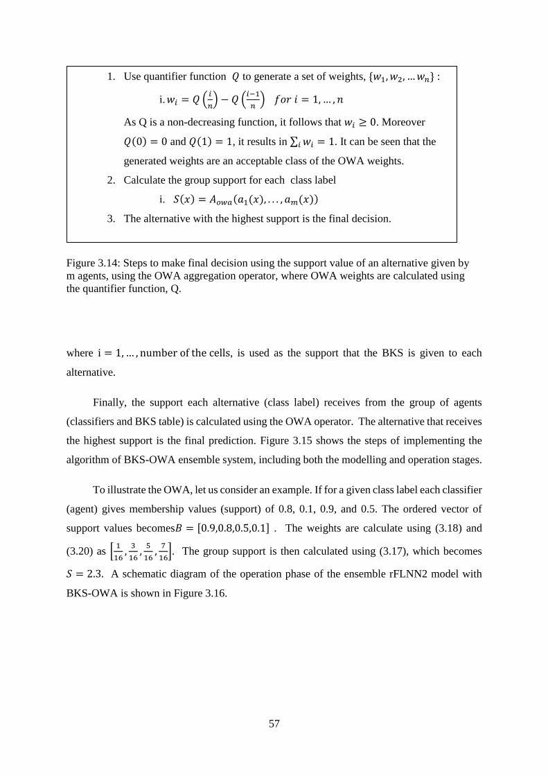
57
Figure 3.14: Steps to make final decision using the support value of an alternative given by
m agents, using the OWA aggregation operator, where OWA weights are calculated using
the quantifier function, Q.
where i = 1,… , number of the cells, is used as the support that the BKS is given to each
alternative.
Finally, the support each alternative (class label) receives from the group of agents
(classifiers and BKS table) is calculated using the OWA operator. The alternative that receives
the highest support is the final prediction. Figure 3.15 shows the steps of implementing the
algorithm of BKS-OWA ensemble system, including both the modelling and operation stages.
To illustrate the OWA, let us consider an example. If for a given class label each classifier
(agent) gives membership values (support) of 0.8, 0.1, 0.9, and 0.5. The ordered vector of
support values becomes𝐵 = [0.9,0.8,0.5,0.1] . The weights are calculate using (3.18) and
(3.20) as [1
16,3
16,5
16,7
16]. The group support is then calculated using (3.17), which becomes
𝑆 = 2.3. A schematic diagram of the operation phase of the ensemble rFLNN2 model with
BKS-OWA is shown in Figure 3.16.
1. Use quantifier function 𝑄 to generate a set of weights, {𝑤1, 𝑤2, …𝑤𝑛} :
i. 𝑤𝑖 = 𝑄 (𝑖
𝑛) − 𝑄 (
𝑖−1
𝑛) 𝑓𝑜𝑟 𝑖 = 1,… , 𝑛
As Q is a non-decreasing function, it follows that 𝑤𝑖 ≥ 0. Moreover
𝑄(0) = 0 and 𝑄(1) = 1, it results in ∑ 𝑤𝑖𝑖 = 1. It can be seen that the
generated weights are an acceptable class of the OWA weights.
2. Calculate the group support for each class label
i. 𝑆(𝑥) = 𝐴𝑜𝑤𝑎(𝑎1(𝑥), . . . , 𝑎𝑚(𝑥))…
3. The alternative with the highest support is the final decision.

58
Algorithm: rFLNN2 based ensemble model with BKS-OWA
Input:
a. Number of classifiers: 4
b. Number of classes : K
c. Training patterns
d. Quantifier function : 𝑄(𝑟) = 𝑟2
Output: FLNN ensemble classification system and set of final decisions
Begin:
Division of data set
The dataset is divided into two parts: training and testing
I. Knowledge modelling:
For four types of basis functions (i.e. polynomial, trigonometric, Legendre, and Chebyshev):
Build the rFLNN2 classifiers
Build rFLNN2 according to section3.3
Build BKS table
Initialize Nunit = K(number of classifiers) BKS units , such that each unit have 𝐾 empty cells
Generate decision combination for each training sample
Use the decision combination and the true class of each sample to populate the cells of BKS
units
II. Operation
For each test sample:
Generate decision combination
Present each test sample to the four rFLNN2 individual classifiers and use the outputs to
generate decision combination
Find focal unit
Using the decision combination find the focal unit which is the BKS unit that has the same
decision combination
Rejection criteria
Check if the focal unit is not empty proceed to the below otherwise classify the sample as
rejected
Check if the best representative class of the unit is unique select it as final decision, otherwise
classify it as rejected
…

59
Figure 3.15: Algorithm representation of ensemble rFLNN2 model
For each rejected sample:
Calculate support values for each class
The quantitative degrees of membership to each class from each classifier is considered as the
support value
If the focal unit of the sample is not empty, the support of BKS table is calculated using
Equation ( 3-18 )
Order support values
Order the support values in a descending manner
Calculate weight values of OWA operator
Use quantifier function Q and Equation (3-16)
Calculate group support value
Having all weights and ordered support values calculate the group support value for each class
using ordered weighted summation
Generate final decision
Generate final decision for initially rejected sample by selecting the class that its group
support value is maximum
End

60
Figure 3.16: Schematic diagram of operation phase in BKS-OWA ensemble model.𝜑3
indicates the degrees of membership to each class (Section 2-7)
3.5 Chapter Summary
The FLNN is the core of the models developed in this thesis. As such, this chapter starts with
describing the details of deploying the FLNN for solving a general classification problem. It
includes describing four FLNNs with polynomial, trigonometric, Chebyshev and Legendre
basis functions.
An evolutionary approach has been proposed in order to optimize the architecture of
the FLNN. More specifically a framework is designed using the GA to generate FLNN with

61
parsimonious topologies. Two corresponding models are developed. In the first model, which
is called rFLNN1, the structure of the FLNN is encoded to a binary chromosome while BP
algorithm is used for tuning the weights of the FLNNs during fitness evaluation of the
chromosomes.
For the second model, rFLNN2, the rFLNN1 is modified such that both the weight
tuning and architecture tuning are handled simultaneously. This model benefits from the key
advantage of the FLNNs which is their one layer nature, and formulates the problem of finding
the compact FLNN into a single objective problem. In order to handle the corresponding search
space with GA the problem is encoded to chromosomes that have binary genes as well as real-
valued genes. As such, novel mutation operator and cross over operator are introduced to be
able to deal with the mixed- type chromosomes.
Using a group of networks to solve a problems is a popular approach in ANN research
community. The diversity between FLNNs with different basis functions (namely polynomial,
trigonometric, Legendre, and Chebyshev) is considered for proposing an FLNN-based
ensemble system. The ensemble model combines the class label output of the individual.
rFLNN2 classifiers using the BKS decision combination method. It proposes a framework in
which an OWA operator with linguistic quantifier works in accordance with the BKS
combination method to make the final decision for all the test samples.

62
Experimental Results, Analysis, and Discussion
The individual and ensemble FLNN- based models proposed in Chapter 3 are evaluated
thoroughly through a series of systematic and comprehensive experiments. In this chapter,
details of the experiments, which include the data sets, experimental settings, and evaluation
metrics, are described. First the results of experiments using the benchmark datasets are
described, which includes the comparative studies of the models. Then the results of solving
two real world problems using the proposed ensemble model is given and discussed. Section
4.4 describes the results of solving several benchmark classification tasks using four FLNN
variants, namely power polynomial (p-FLNN), trigonometric (tr-FLNN), Legendre (Le-
FLNN), and Chebyshev (Che-FLNN), are given and discussed. All four classifiers are used to
solve clean data sets as well as noise contaminated datasets. Then their performance is
compared using a statistical significant test [176].
The experiments conducted using the rFLNN1 and rFLNN2 models are explained in
Section 4.6, where the obtained results are discussed to evaluate the usefulness of the proposed
models as well as their limitations. Section 4.7 describes the results of experiments concerning
the rFLNN2 ensemble classification system. For confirming the usefulness of the proposed
models, the performance of each model is compared with those from related works found in
the literature. The rFLNN1 model is compared with a hybrid FLNN (HFLNN) model [170]
and rFLNN2 model is compared with an evolutionary FLNN (EFLNN) model [78]. The results
show that the performance of rFLNN1 is as good as or better than HFLNN for most of the
comparison cases. The comparison results for rFLNN2 shows that it performs satisfactory and
promising. The performance of rFLNN2 ensemble model is compared with other 8 ensemble
models. Moreover, the performance of BKS-SB and BKS-OWA systems are evaluated through
the experiments. The results indicate the superiority of BKS-OWA system in handling the
rejected samples.
Finally in section 4.8 the ensemble model is used to solve two real world problems. One
of which deals with the power quality evaluation [177] , and the other one deals with the fault
detection in induction motors[178]. The results show the promising performance of the
developed ensemble classification model in handling the real world problems.

63
4.1 Description of Benchmark Data Sets
A total of twelve benchmark data sets are selected for experiments. All these data sets are
publically available from the UCI machine learning repository [179]. Diverse data sets from
different domains are used to evaluate the proposed rFLNN-based models. They differ in terms
of the number of classes, number of samples, and input dimensionality. Specifically, six data
sets have low input dimension (< 10) while the remaining six have high input dimension (10
<=dimension <=33) Each group consists of one binary classification problem, with the rest
involve multi-class problems. A brief description of each data set is as follows.
Wisconsin Breast Cancer (WBC): This data set contains cases from a study conducted at the
University of Wisconsin Hospitals, Madison. The data samples were collected from patients
who had undergone surgery for breast cancer. The task is to determine whether the detected
tumor is benign or malignant. A total of nine predictive features are computed from a digitized
image of a fine needle aspirate (FNA) of a breast mass. They describe the characteristics of the
cell nuclei present in the image [180]. The attributes are as follows:
Radius (mean of distances from center to points on the perimeter)
Texture (standard deviation of gray-scale values)
Smoothness (local variation in radius lengths)
Compactness of the cell nuclei
Concavity (severity of concave portions of the contour)
Concave points (number of concave portions of the contour)
Symmetry
Fractal dimension
Class : (M = malignant, B = benign)
Dermatology: This data set addresses the problem of differential diagnosis of Eryhemato-
Squamous diseases. There are six diseases to be distinguished, namely psoriasis, seboreic
dermatitis, lichen planus, pityriasis rosea, cronic dermatitis, and pityriasis rubra pilaris. A total

64
of thirty-four features are provided, in which thirty-three of them are linear and one of is
nominal. The detailed description of the features can be found in [179].
E.Coli: Escherichia coli describes a protein localization problem. The data set was created by
Institute of molecular and cellular biology of Osaka University. It has seven predictive
attributes calculated from the amino acid sequences, as follows:
mcg: McGeoch's method for signal sequence recognition.
gvh: Von Heijne's method for signal sequence recognition.
lip: Von Heijne's Signal Peptidase II consensus sequence score, (binary attribute).
chg: Presence of charge on N-terminus of predicted lipoproteins, (binary attribute).
aac: Score of discriminant analysis of the amino acid content of outer membrane and
periplasmic proteins.
alm1: Score of the ALOM membrane spanning region prediction program.
alm2: Score of ALOM program after excluding putative cleavable signal regions from
the sequence.
Class: The localization site of protein (cytoplasm, inner membrane without signal
sequence, periplasm, inner membrane, un-cleavable signal sequence, outer membrane,
outer membrane lipoprotein, inner membrane lipoprotein, inner membrane, cleavable
signal sequence)
The detailed description is presented in [181].
Glass: This data set represents a six glass types identification problem. It contains nine input
features and the class attribute. The input features are as follows:
RI: refractive index
Weight percentage of the corresponding oxides in:
Na: Sodium
Mg: Magnesium
Al: Aluminum
Si: Silicon
K: Potassium
Ca: Calcium

65
Ba: Barium
Fe: Iron
Class (type of glass): building_windows_float_processed, building_windows, vehicle
windows, containers, table ware , headlamps.
Ionosphere: This data set contains signals collected from a radar in Goose Bay, Labrador. The
signals were processed using an autocorrelation function with time of the pulse and pulse
number as argument. It contains thirty-three predictive features and a binary class attribute
(“Good” versus “Bad” signals). The Good signals are those indicating some type of structure
in the ionosphere, while the Bad one are those do not. All thirty-three features are continuous
numeric values. The detailed description about them can be found in [182] .
Iris . This is an Iris plant classification data set. The task is to discern among three types of
flowers, based on 4 physical properties of the plant, as follows:
Sepal length (cm)
Sepal width (cm)
Petal length (cm)
Petal width (cm)
Class: Setosa, Versicolour, Virginica
Page Blocks: This problem is concerned with classifying all the blocks of the page layout of
a document according to ten features obtained by a segmentation process. A description of
each feature is as follows:
height: Height of the block
length: Length of the block
area: Area of the block (height * length)
eccen: Eccentricity of the block (length / height)
p_black: Percentage of black pixels within the block (blackpix / area)
p_and: Percentage of black pixels after the application of the Run Length
Smoothing Algorithm (RLSA) (blackand / area)
mean_tr: Mean number of white-black transitions (blackpix / wb_trans)
blackpix: Total number of black pixels in the original bitmap of the block

66
blackand: Total number of black pixels in the bitmap of the block after the RLSA
wb_trans: Number of white-black transitions in the original bitmap of the block
class: text, horizontal line, picture, vertical line, graphic
Pima Indian dataset (or diabetes data set): This data set contains 768 instances taken from a
larger set of data, considering several constrains. All selected patients are female, who are at
least 21 years old, and they are of Pima Indian heritage. The task is to predict whether the
patient would develop diabetes within the next five years. Each sample data consists of eight
real-valued medical attributes, and the last attribute is the class value:
Number of pregnancies
Plasma glucose concentration
Glucose tolerance test
Diastolic blood pressure (mmHg)
Triceps skin fold thickness (mm)
2 Hour serum insulin (mu U/ml)
Body mass index (weight in Kg/(height in m)^2)
Diabetes pedigree function
Age (years)
Class (0 or 1)
Segmentation: This problem involves image segmentation data taken randomly from seven
outdoor image databases. Each sample encodes a three-by-three pixel region. The task is to
classify each instance into 7 classes. A total of 19 continuous input features are available as
follows:
The column of the center pixel of the region,
The row of the center pixel of the region.
the number of pixels in a region = 9.
short-line-density-5: the results of a line extractoin algorithm that counts how many
lines of length 5 (any orientation) with low contrast, less than or equal to 5, go through
the region.
Number of high contrast, greater than 5
Mean of the measure of the contrast of horizontally adjacent pixels in the region.

67
Standard deviation of the measure of the contrast of horizontally adjacent pixels in the
region
Mean of the measures of the contrast of vertically adjacent pixels
Standard deviation of the measures of the contrast of vertically adjacent pixels
Average of the intensity over the region; (R + G + B)/3
Average of the R value over the region
Average of the B value over the region
Average of the G value over the region
Measure of the excess red: (2R - (G + B))
Measure of the excess blue: (2B - (G + R))
Measure of the excess green: (2G - (R + B))
3-d nonlinear transformation of RGB. (obtained according to the algorithm in [183]
Mean of the above saturation
Mean of the hue value.
Class : brickface, sky, foliage, cement, window, path, grass
Thyroid: Among the several data sets available about the Thyroid disease, the one including
215 instances is used throughout this research. This data set is also known as the “new thyroid”
dataset in the literature. The task is to determine, for a given patient, whether he/she is normal
or suffers from hyper/ hypo-thyroidism. The input features are as follows:
T3-resin uptake test result. (in percentage)
Total Serum thyroxin as measured by the isotopic displacement method.
Total serum triiodothyronine as measured by radioimmune assay.
Basal thyroid-stimulating hormone (TSH) as measured by radioimmune assay.
Maximal absolute difference of TSH value after injection of 200 micro grams of
thyrotropin-releasing hormone as compared to the basal value.
Class attribute ( normal, hyper, hypo)
Vowel: This problem involves recognition of eleven vowels of British English. Each one is
part of a word made by several speakers. It has ten numeric predictor features as follows
Class: (vowels involved in the words: ) heed (i), hid (I), head (E), had (A), hard (a:), hud (Y),
hod(O), hoard (C:), hood (U), who’d (u:), heard (϶:)

68
Wine: This data set contains the results of a chemical analysis on wines grown from three
different cultivars in a region in Italy. The results include the amount of thirteen constituents.
There are 178 instances, and the task is to classify them into three groups of wines. The thirteen
predictive features and class attribute are as follows:
Alcohol
Malic acid
Ash
Alkalinity of ash
Magnesium
Total phenols
Flavonoids
Neoflavanoid phenols
Pro anthocyanins
Colour intensity
Hue
OD280/OD315 of diluted wines
Proline
Class: Three different types of wine represented as 1,2, and 3.
Yeast: This data set also involves a protein localization site problem [184]. A total of 1484
proteins are classified into 10 classes. Each pattern is composed of eight predictive features,
calculated from the amino acid sequences, as follows:
mcg: McGeoch's method for signal sequence recognition.
gvh: Von Heijne's method for signal sequence recognition.
alm: Score of the ALOM membrane spanning region prediction program.
mit: Score of discriminant analysis of the amino acid content of the N-terminal region
(20 residues long) of mitochondrial and non-mitochondrial proteins.
erl: Presence of "HDEL" substring (thought to act as a signal for retention in the
endoplasmic reticulum lumen). Binary attribute.
pox: Peroxisomal targeting signal in the C-terminus.
vac: Score of discriminant analysis of the amino acid content of vacuolar and
extracellular proteins.

69
nuc: Score of discriminant analysis of nuclear localization signals of nuclear and non-
nuclear proteins.
The key characteristics of all described data sets are summarized in Table 4.1. For each data
set, the number of samples, number of features, number of classes, and number of samples per
each class are shown.
Table 4.1: Summary of the benchmark data sets employed in the experimental study
Data set No. of
Samples
No. of
Features
No. of
Classes
No. of Samples per class
Input D
imen
sion <
10
Binary Breast
C.W.
699 9 2 241/458
Multi-
Class
Iris 150 4 3 50/50/50
Thyroid 215 5 3 150/35/30
Glass 214 9 6 70/76/17/13/9/29
E.Coli 336 7 8 143/77/2/2/35/20/5/52
Yeast 1484 8 10 244/429/463/44/35/51/163/30/20
/5
10≤
Input D
imen
sion
≤3
3
Binary Ionosphere 351 33 2 225/126
Multi-
Class
Wine 178 13 3 59/71/48
Page
Blocks
5472 10 5 4913/ 329/ 28 /87/ 115
Segment 2310 19 7 161/162/159/159/161/159/161/15
8/155/158
Vowel 990 10 11 90/90/90/90/90/90/90/90/90/90/9
0
4.2 Noisy data
To further evaluate the proposed rFLNN-based models, a series of experiments using noise
contaminated data are conducted as well. Three noise contamination scenarios have been
considered in this research, as follows:

70
I. Noise in both training and test data samples, (denoted as noisy-noisy)
II. Noise only in the test data samples, (denoted as clean-noisy) and
III. Noise only in the training data samples (denoted as noisy-clean).
For each scenario, noise is added to the features, i.e., a certain percentage (e.g. 20%) of the
feature is replaced with a random uniformly generated from the range of that feature. The
noisy data sets are taken from the KEEL repository [185] and used for evaluation in this
research.
4.3 Performance Metrics
For the empirical evaluation in this research, the performance metrics used are as
follows.
Accuracy: accuracy (i.e. the percentage of correctly classified samples) is a common metric to
evaluate classification models.
The overall accuracy of multi-class classification is the sum of individual class accuracy
rates, as follows
Accuracy =1
𝑇𝑠∑ 𝑀𝑖𝑖
𝑁𝑖=1 (4-1)
where 𝑀𝑖𝑖 is the true positive predictions for each class and 𝑇𝑠 is the total number of samples
in the evaluation set.
Cross validation: Cross-validation is a technique to evaluate predictive models by
partitioning the original samples into a training set for training the model, and a test set for
evaluation.
In k-fold cross-validation, the original set of samples is randomly partitioned into k subsets.
Each subset contains an approximately equal number of samples. A total of K-1 sub sets are
used for training the model, and the one remaining is used for testing the model. The cross-
validation process is then repeated k times (equal to the number of the folds). In each repetition,
a new subset is considered for validation, while others used for training the model. As such, k
results are produced, which are averaged to give an overall performance metric. In the cross-
validation method all samples are used for training and evaluation, and each of which is utilized

71
for evaluation only once. Figure 4.1 is a schematic representation of the k-fold cross-
validation.
Figure 4.1: Schema of k-fold cross validation
For classification problems, stratified k-fold cross-validation is used, in which the folds
are selected so that each fold contains roughly the same proportions of class labels. Generally
in this research, a 5−fold cross validation is carried out to evaluate the proposed models. The
corresponding average and standard deviation of performance metrics are recorded and
analysed. However, in certain comparative studies, the experimental procedures follow those
reported in the literature, in order to have a fair comparison.
4.4 Comparison of Two Classifiers
In order to compare different algorithms and to show whether there exist significant
differences among them, a statistical comparison is required [176]. In this research, a non-
parametric test, i.e., the Sign test [176, 186, 187], is adopted. To compare the overall
performance of algorithms, the number of cases on which an algorithm is the overall winner is
counted. These counts are used in inferential statistics, with forms a two-tailed binomial test,
namely the Sign test [188]. If both compared algorithms are equivalent, as assumed under the
Iteration 1
Iteration 2
. . . . . .
. . . . . .
. . .
Iteration k
Training
Testing
All data

72
null hypothesis, each should win on approximately 𝑛/2 out of n problems. The number of wins
is distributed according to a binomial distribution, which allows the use of the z-test [176].
Table 4.2 shows the critical number of wins needed to achieve both 𝛼 = 0.05 (95%
confidence) and 𝛼 = 0.1 (90% confidence) levels of significance [176]. Note that, since tied
matches support the null hypothesis, they should not be discounted when applying this test, but
split evenly between the two algorithms; if there is an odd number of them, one should be
ignored.
Table 4.2: Look up table for the two-tailed sign test at 0.05 and 0.1 levels of significance
[176]
#cases 5 6 7 8 9 10 11 12 13 14 15 16
𝛼 = 0.05 5 6 7 7 8 9 9 10 10 11 12 12
𝛼 = 0.1 5 6 6 7 7 8 9 9 10 10 11 12
4.5 FLNNs with different basis functions
In this section, the evaluation results of four FLNN classifiers namely, FLNN with
polynomial basis function (p-FLNN), FLNN with trigonometric basis function (tr-FLNN),
FLNN with Legendre basis function (Le-FLNN), and FLNN with Chebyshev basis function
(Ch-FLNN), are presented. The corresponding experiments have been carried out using both
clean and noisy data sets. The R2015b version of Matlab programming language has been used
to develop these FLNN models and conduct the respective experiments.
For the experiments, 12 data sets from the Knowledge Extraction based on Evolutionary
Learning (KEEL) repository are considered. This repository maintains several benchmark data
sets, originally taken from UCI [179] . The data sets are organized in various categories of
data mining tasks like classification, regression and time series analysis. Classification data
sets are provided in both clean and noisy versions. They are presented in complete format as
well as in stratified 5−fold and 10−fold partitioned formats. For noisy data sets, different
levels of noise are added to the features or to the class labels. The sample ordering remains
the same for clean and noisy data sets, which makes comparison of different algorithms
consistent. To run the experiments of this section the 5-fold partitioned of clean and 20% noise
level data sets are selected for conducting the experiments.

73
Table 4.3, Table 4.5,Table 4.7,Table 4.9 summarize the mean accuracies obtained by four
FLNNs through a 5-fold cross validation procedure. Table 4.3 shows the results using the clean
data, while the other tables describe the results of noisy data. In each experiment the average
of performance over low dimensional and high dimensional problems is calculated. While to
compare the performance of FLNNs statistically, the number of wins and losses of the FLNN
over all problems is counted and the statistical sign test has been conducted (according to
Table 4.2). The sign test results on the clean and noisy datasets are summarized in
Table 4.4,Table 4.6,Table 4.8 and Table 4.10. In each of which the significantly better FLNN
and the detected level of significance is reported.
Results and discussion for FLNNs experiments
Table 4.3 shows the average test accuracy of four FLNN classifiers on clean data. The overall
results indicate that, the optimal choice of basis function is problem dependant. As an instance,
in case of Ecoli, the trigonometric basis function is the best option, while for Vowel, the
polynomial basis function performs the best. Theoretically, it is obvious that using a basis
function that is closer to the underlying distribution function of the data could result in a better
FLNN, but it requires prior domain knowledge.
Table 4.3: Test Accuracies of FLNN classifiers with different basis functions, over 5-fold
dataset taken from KEEL repository :
Data set p-FLNN tr-FLNN Le-FLNN Ch-FLNN
Breast C.W. 95.78 96.33 96.64 96.94
Iris 97.67 96 97.29 96.18
Input
dimension<10 Thyroid 94.13 94.23 94.21 94.32
Glass 64.25 66.31 62.24 62.11
Ecoli 58.51 81.55 57.56 32.07
Yeast 59.41 60.29 58.7 58.93
Average 78.29 82.45 77.77 73.42
Ionosphere 92.43 92 92.14 91.38
Wine 96.24 96.65 96.91 96.93
10≤ Input
dimension ≤33 Page Blocks 95.06 94.52 94.59 94.58
Dermatology 97.02 97.21 97.49 97.44
Segmentation 90.06 91.8 89.11 88.77
Vowel 77.39 74.35 68.08 67.74
Average 91.37 91.09 89.72 89.47

74
Moreover the performance of the FLNN models with different basis functions are grouped into
two, i.e., low (<10) and high (between 10 and 33) input dimension problems. The average
results over low dimensional and high dimensional problems (Table 4.3) show that, on average,
the tr-FLNN model performs better than other three models, and the Ch-FLNN model produces
the worst results. To statistically validate this observation, a statistical hypothesis test on the
performance over all data sets is conducted. The results are shown in Table 4.4.
Table 4.4: Statistical sign test results for significance levels of 𝛼 = 0.05 and 𝛼 = 0.1.
P-FLNN TR-FLNN LE-FLNN CH-FLNN
P-FLNN Not statistically
different
Not statistically
different
Not statistically different
Detected
differences
TR-
FLNN
Not statistically
different
Not statistically different
Detected
differences
LE-FLNN Not statistically different
Detected
differences
CH-
FLNN
Detected
differences
Table 4.4 summarise the sign test results for pairwise comparison of four FLNN models
in solving twelve classification problems with significance levels of 𝛼 = 0.05 and 𝛼 = 0.1.
According to pairwise comparison outcome, no significant difference can be observed for the
four FLNN models in tackling all twelve problems.
Figure 4.2 represents the test accuracy of each FLNN on the datasets. It indicates that
the general trend is the same for all FLNNs. In other words, a complicated problem is harder
to solve for almost all FLNN classifiers. All classifiers perform closely well for Thyroid, while
their performances show the most variation in case of E.Coli. On the other hand, the FLNN
with Polynomial basis function gives its best performance for the Iris problem, while the other
three FLNNs perform best for Dermatology. In case of the worst performance, the FLNN with

75
trigonometric basis function performs the worst in case of Yeast, while other three show the
worst performance for E.Coli.
Figure 4.2: Test accuracies of FLNNs with 4 different basis functions on 12 benchmark data
sets
Noisy training and clean test data sets
For noisy training and clean test data, the sign test reveals that p-FLNN performs
significantly better than Ch-FLNN and tr-FLNN at the significance levels of 𝛼 = 0.05 and 𝛼 =
0.1 , respectively. tr-FLNN performs better than Ch-FLNN at the significance level of 𝛼 =
0.05. All other comparisons do not show performance with significant difference.

76
Table 4.5: Average test accuracies and standard deviations for data with 20% level of noise in
training data and clean test
20%NC p-FLNN tr-FLNN Le-FLNN Ch-FLNN
Breast C.W. 96.1 96.44 95.9 95.93
Iris 90 95.33 95.33 96.67
Input dimension<10 Thyroid 87.44 91.63 85.12 86.98
Glass 54.2 54.65 51.4 50.47
Ecoli 53.3 79.48 60.72 44.42
Yeast 51.78 53.15 51.55 51.28
Average 72.13 78.44 73.33 70.95
Ionosphere 88.04 89.18 88.03 87.18
Wine 96.63 95.51 96.63 95.52
10≤ Input dimension
≤33 Page Blocks 92.58 91.67 91.06 91.41
Dermatology 96.44 96.39 96.66 96.14
Segmentation 14.18 83.41 17.06 19.6
Vowel 62.02 62.32 57.68 57.58
Average 74.98 86.41 74.52 74.57
Table 4.6: Pairwise comparison of FLNN classifiers based on their performance over 12 data
sets, using two tailed sign test
P-FLNN TR-FLNN LE-FLNN CH-FLNN
P-FLNN tr-FLNN Not statistically
different
p-FLNN ,
Detected
significance
level
𝛼 = 0.1 𝛼 = 0.05
TR-FLNN Not statistically
different
tr-FLNN,
Detected
significance
level
𝛼 = 0.05
LE-FLNN Not statistically
different
Detected
significance
level
CH-FLNN
Detected
significance
level

77
Clean training, noisy test data sets
For evaluation with clean training and noisy test data, tr-FLNN performs significantly better
than all other three FLNNs at the significance level of 0.05. Other FLNNs do not show
performances with significant difference in pairwise comparisons.
Table 4.7: Average test accuracies for data with clean train and 20% level of noise in test data
20%CN p-FLNN tr-FLNN Le-FLNN Ch-FLNN
Breast C.W. 91.24 94.59 94.6 95.04
Iris 80.67 86 84 85.33
Input dimension<10 Thyroid 66.98 80 77.67 79.53
Glass 49.99 53.69 53.71 55.14
Ecoli 57.62 69.36 64.41 63.82
Yeast 41.41 43.35 43.93 43.14
Average 64.65 71.165 69.72 70.33
Ionosphere 82.45 85.18 87.19 86.05
Wine 78.62 83.65 84.25 83.7
10≤ Input dimension
≤33 Page Blocks 63.12 77.42 69.02 67.74
Dermatology 91.34 92.18 92.16 90.93
Segmentation 14.05 67.05 65.68 57.92
Vowel 45.56 48.89 42.93 43.56
Average 62.52 75.73 73.54 71.65
Noisy training Noisy test data sets
A series of evaluations using noisy data sets for both the training and test sessions has
been conducted with all twelve problems. Table 4.9 presents the obtained classification
accuracy results. Where Table 4.2 shows the sign test results accordingly. It can be seen that
when both training and test data are noisy, tr-FLNN performs better than p-FLNN at the
significance level of 𝛼 = 0.1. It performs better than both Le-FLNN and Ch_FLNN at the
significance level of 𝛼 = 0.05. p-FLNN, Le-FLNN, and Ch-FLNN perform equivalent, up to
the significance level of 𝛼 = 0.1.
Figure 4.3 shows the overall average accuracy of each FLNN for all datasets, with
respect to the different clean/noisy data combinations. In all cases, as expected, adding noise
results in performance degradation. However, when performance degradation is particularly
obvious in clean training and noisy test scenarios. Another observation from Figure 4.3 is that
tr-FLNN generally performs better in noisy data problems.

78
Table 4.8: Pairwise comparison of FLNN classifiers over 20% level of noise in train-clean
test problems
p-FLNN tr-FLNN Le-FLNN Ch-FLNN
P-FLNN Tr-FLNN Le-FLNN Ch- FLNN
Detected
significance
level
𝛼 = 0.05 𝛼 = 0.05 𝛼 = 0.05
Tr-FLNN Not statistically
different
Not statistically
different
Detected
significance
level
Le-FLNN Not statistically
different
Detected
significance
level
Ch-FLNN
Detected
significance
level
Table 4.9: Average test accuracies for data with 20% level of noise in both training and test
data
Data set p-FLNN tr-FLNN Le-FLNN Ch-FLNN
Breast C.W. 94.7 95.39 95.29 95.56
Iris 87.22 84.89 82.31 78.33
Input dimension<10 Thyroid 77.21 83.26 77.67 77.67
Glass 52.78 55.13 55.59 53.72
Ecoli 64.29 70.25 66.07 64.57
Yeast 43.95 46.52 43.93 44.2
Average 70.02 72.57 70.14 69.00
Ionosphere 86.63 86.9 81.78 80.56
Wine 88.76 88.73 85.95 88.22
10≤ Input dimension
≤33 Page Blocks 90.86 90.46 90.41 90.39
Dermatology 89.57 91.45 92.27 91.9
Segmentation 77.55 82.75 80.09 79.86
Vowel 42.63 44.04 38.79 38.99
Average 79.33 80.72167 78.215 78.32

79
Table 4.10: Pairwise comparison of FLNN classifiers for 20% of noise in train and test data,
using two tailed sign test with 𝛼=0.05, and 0.1 level of statistical significance
P-FLNN Tr-FLNN Le-FLNN Ch-FLNN
P-FLNN Tr-FLNN Not statistically
different
Not statistically
different
Detected
significance
level
𝛼 = 0.1
Tr-FLNN Tr-FLNN Tr-FLNN
Detected
significance
level
𝛼 = 0.05 𝛼 = 0.05
Le-FLNN Not statistically
different
Detected
significance
level
Ch-FLNN
Detected
significance
level
Figure 4.3: Average of average accuracies with different noise placements in train and test
sets respectively
0
10
20
30
40
50
60
70
80
90
100
P-FLNN Tr-FLNN Le-FLNN Ch-FLNN
Average Performance of FLNN classifiers
clean-clean noisy-clean clean-noisy noisy-noisy

80
Remarks on FLNNs with different basis functions
To perform an in-depth investigation on the FLNN classifiers with different basis functions,
their test performances on the Ecoli problem have been considered. Figure 4.4. It can be seen
that there is diversity among the decisions of FLNNs. In other words, FLNN classifiers with
different basis functions capture different aspects of knowledge from the data set. This
understanding motivates the development of an ensemble model using these four FLNN
classifiers, as presented in section 3.4.
Figure 4.4: True class labels and class predictions by P-,tr-,Le-,and Ch- FLNN classifiers for
67 test samples of Ecoli problem in a fold
4.6 rFLNN Models
In this section the results of a comparative study for rFLNN1 and rFLNN2 models are
given. For this purpose, two closely related publications in the literature, i.e., [32] and [78],
have been used for performance comparison. To ensure fairness, the experimental procedures
follow those used in [82] and [81], which include the data sets and their partitions as well as
evaluation settings.

81
Experimental Procedure for rFLNN1
The rFLNN1 model is compared with three similar models , namely Hybrid FLNN
(HFLNN)[32], standard FLNN, and the radial basis function network (RBF) from [55]. Both
rFLNN1 and standard FLNN have been extensively described in Chapters 2 and 3. A
description of the HFLNN model is given, as follows, while its details can be found in the
original paper of HFLNN [55].
The HFLNN model [32, 55] selects an optimal subset of the original features using a
feature selection procedure. The original feature subsets are optimized by evolution through a
GA. In the designed GA, each individual represents a selected subset of original features with
a binary chromosome. An FLNN model is then built using that subset. The cost value
associated with each individual includes a combination of the classification error of that FLNN
over training data, and also the number of selected features. As such, the fittest individual
represents the FLNN with the best classification performance, and with the least number of
features. The schema of this HFLNN model is shown in Figure 4.5.
Figure 4.5: Schematic diagram of HFLNN proposed in [32] vs. rFLNN1 with the same basis
functions

82
rFLNN1 Configurations
Basis functions: As described in Chapter 3, rFLNN1 can be built with any basis
function. However, for the comparative study, the trigonometric function is adopted, which is
in accordance with that in the HFLNN model [55]. Moreover, the same data sets and cross
validation settings of HFLNN in [137] have been followed for a fair comparison.
GA parameters: The GA population size is problem dependant [189]. After a few trails and
error evaluation, it is set to three times of the length of an individual for each problem.
The crossover probability is set to 0.8 and the mutation probability is set to 0.05 for all
experiments. These values have been determined after several trials.
Cross validation: The same data sets and cross validation settings of HFLNN in [137] have
been followed for a fair comparison. A two-fold cross validation procedure has been used for
all data sets. Each data set is randomly divided into two subsets. Each subset is alternatively
used for training and test. Since the GA and FLNN are stochastic in nature, each experiment
has been repeated thirty times, and the average test accuracy rates are calculated.
Results of the rFLNN1 Evaluation
Table 4-11Table 4.1: Summary of the benchmark data sets shows the performance of
rFLNN1 with respect to its average testing accuracy rates on eight data sets. The results are
compared with those of HFLNN, standard FLNN and RBF models [15]. It can be observed that
in all problems, except IRIS, rFLNN1 performs better than three other models. In the case of
IRIS, HFLNN and standard FLNN yield the best performances of 97.33% and 96.33%
accuracy rates, respectively. The rFLNN1 model achieves 94.00% average test accuracy.
Based on the statistical sign test [176], rFLNN1 performs significantly better than the other
three models at the significance level of 𝛼 = 0.05.
Table 4-12 as well as Figure 4.6 show the comparative results between rFLNN1 and other
models with respect to test accuracy at maximum train accuracy achieved for each data set.
For all data sets, rFLNN1 outperforms other models in terms of training and test accuracy
rates. With the Zoo data set, all models can achieve 100% accuracy on training data; however
rFLNN1 gives the best performance for test data of Zoo.

83
Table 4-11: Performance (2-fold cross validation test accuracy) comparison of proposed
rFLNN1 and three other models with eight benchmark data sets
Dataset rFLNN1 HFLNN FLNN RBF
1 Iris 94.00 97.33 96.66 38.50
2 Wine 92.40 90.45 88.76 79.21
3 Pima 76.45 72.14 72.14 76.04
4 Bupa 69.82 69.28 69.28 66.95
5 Ecoli 76.57 50.08 47.31 26.11
6 Glass 64.67 51.51 50.38 34.64
7 Lymph. 78.79 77.03 74.32 72.29
8 Zoo 91.75 86.19 85.16 81.08
The results empirically indicate that rFLNN1, which performs feature selection in the
expanded feature space, is more efficient than HFLNN, which performs feature selection in the
original feature spaces; therefore ascertaining the usefulness of the methodology adopted in
this research for improving the FLNN model in data classification tasks. Figure 4.6 shows the
overall training and test accuracy rates.
Figure 4.7 represents the fraction of expanded features that have been discarded by
rFLNN1 for each data set. It can be observed that up to half of the expanded features are
discarded by rFLNN1. Recalling the original FLNN structure (Figure 2.5), this means
reduction in the number of network parameters by half, because, as stated in Chapter2, there is
a one to one correspondence between the numbers of expanded features and the network
parameters in original FLNN.
The fewest number of expanded features discarded occurs with the Wine data, which
is at 11%. For Lymph and Zoo data sets, rFLNN1 has more than 50% fewer expanded features,
as compared with those in original FLNN used to solve these problems.

84
Figure 4.6: Performance comparison (bottom) with respect to maximum training accuracy
(top)

85
Table 4-12: Comparative performance study w.r.t. maximum train accuracy / test accuracy
Max train accuracy/test accuracy
Dataset rFLNN1 HFLNN FLNN RBF
Iris 100/97.33
98.67/97.33 98.67/97.33 57.33/48.00
Wine 100/94.44
100/91.01 97.75/93.26 86.51/82.02
Pima 84.74/75.41
81.51/72.66 80.21/72.66 78.12/77.60
Bupa 84.97/68.61
77.91/70.35 78.49/70.93 71.68/68.21
Ecoli 83.04/81.25 59.83/54.70 52.14/52.14 38.46/27.43
Glass 89.72/59.81 63.81/57.14 60.95/55.05 53.21/38.09
Lymph. 100/79.73
97.30/78.38 94.60/77.03 86.49/75.68
Zoo 100/96.02
100/87.75 100/85.71 100/84.62
Figure 4.7: Fraction of discarded expanded features

86
Remarks on rFLNN1 model
The proposed rFLNN1 model utilizes the GA for feature selection in the expanded
feature space. Then, the BP algorithm is employed for weight tuning. The experimental results
confirm that feature selection in the expanded feature space is an effective strategy to prune the
structure of original FLNN, and to achieve either similar or higher accuracy rates as compared
with those using all the original features. In the experiments, more than half of the expanded
features have been eliminated. This confirms that rFLNN1 is effective and efficient in terms
of classification performance and computational requirement.
Experimental Procedure for rFLNN2
The performance of rFLNN2 is compared with three models, namely, an evolutionary
FLNN model (EFLNN [78]), a constructive algorithm of higher order perceptron (HOP) [78],
and the RBF model [78]. The EFLNN model proposed in [78] uses the polynomial basis
function to expand the original features. It then uses the GA to select an appropriate set of the
polynomial terms. EFLNN uses the BP algorithm to train the resulting network.
The experimental procedure in [78] has been followed in evaluating rFLNN2, and the
polynomial basis function has been selected to construct rFLNN2. Three benchmark
classification problems in [81] are used for evaluation and comparison. Cancer1 and Diabetes1
are extracted from [190]. According to [152], in Cancer1, 525 data samples are used for
training, with the remaining 174 samples used for test, while in Diabetes1, 576 samples are
used for training, with the remaining 192 samples used for test.
The Ionosphere data set is taken directly from the UCI machine learning repository. It
is randomly divided into two sets, one with 276 samples for training and another with 192
samples for test. This data set is selected for experimentation in order to compare the
performance of rFLNN2 with the HOP model. In HOP, real-valued data are approximated by
Boolean functions, and the resulted Boolean data are used to train the HOP model [78].
Results of the rFLNN2 Evaluation
Table 4.8 shows the average test accuracy results of a two-fold cross validation using the
partitioning setting described earlier.

87
Table 4-13: Comparative results of rFLNN2
Dataset rFLNN1_poly rFLNN2 EFLNN HOP RBF
Cancer1 98.33
98.35
98.85 -- --
Diabetes1 75.26
75.39
78.08
-- 75.7
Ionosphere 94.78
95.32
94.27 94.7 --
From the results, both rFLNN2 and EFLNN perform better than HOP and RBF for the
selected problems. In particular, while rFLNN2 outperforms EFLNN in Ionosphere, EFLNN
performs better than rFLNN2 in Cancer1 and Diabetes1.
Figure 4.8: Percentage of weights in rFLNN2 and EFLNN models compared to that in
original FLNN. The difference in performance of rFLNN2 and EFLNN in term of optimising
the standard FLNN structure is significant for Diabetes1. Both models perform equally well
in Cancer1 and Ionosphere. In general, EFLNN outperforms rFLNN2 in term of network
pruning. This could be due to the more complex search space in rFLNN2, whereby the search
space of rFLNN2 covers both the expanded features and network weights. On the other hand,
EFLNN deals with only the search problem pertaining to the expanded features, and optimises
the weights using the BP algorithm. This indicates that further research on enhancing rFLNN2
is necessary, e.g. using other evolutionary or swarm intelligence-based optimising methods, as
highlighted in further research in the next chapter.
4.7 Ensemble rFLNN2 Model
The proposed rFLNN2 ensemble model coupled with the BKS and BKS-SB and BKS-
OWA combination methods are evaluated thoroughly in this section. Firstly, the performances
of the ensemble with standard BKS method is evaluated based on 12 benchmark classification
problems. Clean and noise-contaminated data sets are used for experimentation. Then, the
performances of the ensemble with BKS-SB and BKS-OWA systems are compared. Finally,
the performance of the proposed rFLNN2 ensemble model is evaluated through a comparative
study with eight other ensemble classification methods reported in a recent study [153].

88
Figure 4.8: Percentage of weights in rFLNN2 and EFLNN models compared to that in
original FLNN
Experimental Procedure for the rFLNN2 Ensemble Model
For the first and second parts of the evaluation, the 12 data sets from the KEEL
repository [185], in both clean and noisy versions, are used. The results are based on the 5-fold
cross validation method and the noise level at 20% is used. Three noise-corrupted scenarios,
i.e. noise in both training and test sets, noise only in the training set, and noise only in test set,
are adopted. The performance metrics are the average test accuracy rates over 5 folds and the
rejection rate of the standard BKS combination method.
Results and Discussion of the rFLNN2 Ensemble Model
Table 4.14 to Table 4.17 summarize the experimental results using the proposed ensemble
rFLNN2 model on the benchmark data sets including clean and noisy data. The results include
the ensemble model with the standard BKS method and the BKS-OWA combination method.
The rejection rate of the standard BKS method is also reported. Note that in the BKS-OWA
combination method, the rejection rate is always zero.
0
0.1
0.2
0.3
0.4
0.5
0.6
Cancer1 Diabetes1 Ionosphere
rFLNN2 EFLNN

89
Figure 4.9 and Figure 4.10 depict the classification accuracy and rejection rates of the standard
BKS method, respectively. They represent results for each data set according to various noisy
scenarios, which are clean train-clean test, noisy train-clean test, noisy test-noisy test, and clean
train-noisy test. The highest classification accuracy is yielded from the clean-clean scenario,
which implies that the existence of noise affects classification accuracy. As can be seen from
Figure 4.9, when noise is introduced to corrupt the data samples, a decreasing trend in
classification accuracy
Table 4.14: Five folds cross validation accuracy of rFLNN2 ensemble with normal BKS and
with BKS-OWA combination systems - results for clean datasets five folds
Data set BKS BKS_OWA Rej. Rate (of
BKS method)
1 Breast C.W. .97 49 96.64 1.17
2 Dermatology 98.70 97.49 2.44
3 EColi 89.28 88.30 8.93
4 Glass 69.26 67.90 8.81
5 Ionosphere 94.36 92.61 3.98
6 Iris 97.83 97.89 2.78
7 Page Blocks 95.53 95.02 1.10
8 Segmentation 94.11 92.55 3.33
9 Thyroid 94.35 94.42 1.86
10 Vowel 86.94 80.24 16.11
11 Wine 97.11 95.51 3.95
12 Yeast 60.62 59.56 3.55
Table 4.15: Five folds cross validation accuracy of rFLNN2 ensemble with normal BKS and
with BKS-OWA combination systems- results for noisy train –clean test datasets
BKS BKS_OWA Rej. rate
Breast C.W. 96.69 96.37 0.76
Dermatology 97.66 96.58 3.06
EColi 80.20 65.19 60.31
Glass 57.57 56.05 9.78
Ionosphere 88.14 87.75 1.71
Iris 95.95 94.67 4.00
Page Blocks 92.87 92.87 0.27
Segmentation 50.13 29.76 40.18
Thyroid 92.71 92.09 4.19
Vowel 68.84 64.02 19.83
Wine 97.17 96.63 2.24
Yeast 52.99 52.67 4.61

90
Table 4.16: Five folds cross validation accuracy of rFLNN2 ensemble with normal BKS and
with BKS-OWA combination systems- results for clean train –noisy test datasets
BKS BKS_OWA Rej. rate
Breast C.W. 93.82 93.05 3.27
Dermatology 96.26 93.17 9.07
Ecoli 73.10 65.73 24.62
Glass 52.21 50.83 18.05
Ionosphere 82.16 80.91 5.41
Iris 88.28 83.33 8.67
Page Blocks 72.72 66.68 14.15
Segmentation 56.76 47.85 82.28
Thyroid 83.68 78.14 23.26
Vowel 57.67 51.17 29.13
Wine 85.86 83.68 11.81
Yeast 45.10 42.96 15.26
Table 4.17: Five folds cross validation accuracy of rFLNN2 ensemble with standard BKS
and with BKS-OWA combination systems for noisy train-noisy test datasets
BKS table
accuracy
BKS BKS_OWA Rej. Rate (of
BKS method)
Breast C.W. 97.04 95.76 95.25 1.24
Dermatology 100 94.84 91.68 9.78
EColi 80.36 72.85 70.25 10.71
Glass 75.23 56.03 53.79 12.74
Ionosphere 99.29 87.24 86.91 1.71
Iris 94.17 88.41 85.11 9.00
Page Blocks 91.53 91.03 90.79 0.49
Segmentation 89.40 82.57 80.39 5.46
Thyroid 88.26 83.06 81.86 3.72
Vowel 78.46 48.40 43.03 30.64
Wine 97.19 91.41 88.76 7.89
Yeast 54.16 46.65 45.01 9.60
pertaining to clean-noisy, noisy-clean or noisy-noisy can be observed for all 12 benchmark data
sets, irrespective whether noise is introduced to the training or data sets, or both.
Generally, it can be seen that when both training and test sets are clean (clean train-
clean test), the highest accuracy is achieved, and with the fewest rejected samples. On the other
hand, when the test set is noisy, i.e. noisy train-noisy test and clean train-noisy test, the lowest
accuracy rates are produced, regardless whether the training set is clean or noisy.
The performance of in the clean train-noisy test scenario is inferior to that of noisy
train-noisy test scenario. This indicates that the strategy to eliminate noise-corrupted data from

91
training is not effective, when the test data are subject to noise corruption in practice. The noisy
train-clean test scenario produces the second highest accuracy rates. This indicates that the
ensemble with standard BKS method is able to learn from noisy data (up to 20%), and produces
good results when the test data are clean. For the clean train-noisy test scenario, the highest
rejection rates are observed. In this scenario, the model with standard BKS method contains
no information about the underlying noise distribution, therefore rejects most of the noise-
corrupted test samples.
From Figure 4.10, introducing noise to the training or test data results in an increase of
the rejection rate. When the test samples are noisy (i.e. in both clean train-noisy test and noisy
train-noisy test scenarios), the rejection rate is higher than that of noisy train-clean test scenario.
This, again, indicates that the BKS method is robust against noise (up to 20%) in the training
data). But when the test data are corrupted by noise, the BKS method becomes conservative
and less effective, leading to a high rejection rate.
Evaluation of rFLNN2 Ensemble Model with BKS-OWA and BKS-SB systems
As pointed out in Chapter3, the performance of BKS is compromised by the empty units and
the so-called ambiguous units. When the combined decision of a test sample falls in one of
these units, it is rejected, in order to maintain the generalization error [42]. This can cause a
high rejection rates if many empty or ambiguous units exist. As described earlier in Section
3.4, one way to make decision for rejected samples is accepting the prediction of the single
classifier with higher training accuracy. This results in the BKS-SB system. The OWA operator
based aggregation method is a more elaborate strategy to make decision for rejected samples
which the system is called BKS-OWA accordingly. The effectiveness of both methods is
investigated by comparing their performance using twelve benchmark problems. Table 19
shows the results of 2-fold cross validation.

92
Figure 4.9: 5-fold classification accuracy results for clean train –noisy test datasets
Figure 4.10: 5-fold rejection rate results for data sets with different clean and noisy
configurations.
When the decision is reached using the OWA operator, instead of simply accepting the
best individual classifier’s decision, the performance of BKS-OWA is better in ten out of
twelve problems. As such, BKS-OWA performs significantly better than BKS-SB statistically
at the significance level of α=0.05 .
0
20
40
60
80
100
120
Acc
ura
cy (
%)
clean trainclean test
noisy trainclean test
clean trainnoisy test
noisy trainnoisy test

93
Table 4.18: Test accuracy of rFLNN2 ensemble with BKS-SB BKS- OWA systems. The
higher performance for each problem is bolded.
Data set BKS-SB BKS-OWA
1 Breast C.W. 97.08 97.37
2 Dermatology 95.13 95.80
3 EColi 86.66 87.25
4 Glass 65.11 66.04
5 Ionosphere 92.02 92.14
6 Iris 96.56 97.22
7 Page Blocks 93.68 94.13
8 Segmentation 93.98 94.98
9 Thyroid 93.86 95.26
10 Vowel 90.00 90.90
11 Wine 95.62 95.28
12 Yeast 60.00 59.41
Average 88.31 88.82
The better performance of model with BKS-OWA system is expected as it retains the
knowledge of BKS as well as individual classifiers’ predictions in decision fusion. It also
associates an appropriate weight to the decision of each individual classifier according to its
accuracy during the training phase. On the other hand, BKS-SB system merely considers the
decision from an individual classifier that performs the best during the training phase, and
ignores the information of other classifiers.
Results and Discussion of rFLNN2 Ensemble with BKS-OWA and BKS-SB
systems
The empirical results in the previous section have proven that the proposed BKS-OWA
performs statistically better than BKS-SB. A comprehensive study to evaluate the
effectiveness of the ensemble model with BKS-OWA in handling rejected test samples is
conducted. Specifically, the hypothesis is whether BKS-OWA is able to maintain the accuracy
rate within a 5% limit of those from standard BKS, despite the fact that it does not reject any
sample. The results from both clean and noisy data sets are examined.
Table 4.14 summarizes the results of 5-fold cross validation for clean data sets. BKS-
OWA is able to maintain its accuracy within the 5% limit of those from standard BKS in eleven
out of twelve benchmark problems. In case of IRIS and THYROID problems, model with BKS-
OWA system outperforms the model with standard BKS. From the results, it can be observed

94
that even when the rejection rate is high and standard BKS combination method cannot yield
any prediction for many samples, BKS-OWA system is able to perform with acceptable
accuracy. As an example, in GLASS, a total of 8.82% of test samples are rejected by standard
BKS, and the accuracy obtained for the remaining test samples is 69.26%. BKS-OWA system
provides predictions for all test samples (including the rejected samples) and achieves an
accuracy rate of 67.90%, which is close to that of standard BKS.
Evaluation of rFLNN2 Ensemble Model
A performance comparison between rFLNN2 ensemble model and eight other related
models published in the literature [191] is conducted. The experimental procedure in [153] is
followed, which includes using the same data sets with 2-fold cross validation to evaluate all
models. During the experiments, rFLNN2 ensemble model coupled with BKS-based
combination method is compared against two groups of ensemble methods, as follows.
(A) Conventional Combination Methods
The predictions from individual classifiers in the ensemble are combined using the
conventional combination methods, namely single best as well as majority voting schemes:
Single-best (SB): This scheme selects the best individual classifier in the ensemble and uses its
prediction as the final decision.
Majority voting (MV): This scheme combines the predictions from all classifiers in the
ensemble using the voting strategy, and selects the prediction with the highest vote as the final
decision.
(B) Competence-based Methods
This group includes six competence-based combination methods described in [153], as
follows.
(i) Dynamic Classifier Selection Local Accuracy (DCS-LA): This method defines the
competence of individual classifiers for each test sample using its local classification accuracy.
The local accuracy is calculated based on the 𝑘 = 10 nearest neighbors of the test data in the
training/validation set.
(ii) DCS with Multiple Classifier Behavior (DCS-MCB): This method defines the competence
of the individual classifiers for each test example, x, as the classification accuracy calculated

95
for a data set, 𝑉, which is dynamically generated from the validation data set 𝑉, as follows.
Firstly, the multiple classifier behavior (MCB) is calculated for the test sample, x, and for its 𝑘
nearest neighbours taken from 𝑉. The MCB is defined as a vector with its elements as the
decisions (i.e. class labels assigned to sample 𝑥) of all classifiers in the ensemble. Next,
similarities between the MCB are calculated using the averaged Hamming distance. The
samples in 𝑉 that are most similar to 𝑥 (i.e. below some similarity threshold) are used to
generate the data set 𝑉 [191].
(iii) DCS Modified Local Accuracy (DCS-MLA): This method is similar to DCS-LA, except
the local classification accuracy is estimated using weighted 𝑘 nearest neighbors of the test
example, x, taken from 𝑉.
(iv) Dynamic Ensemble Selection Knora Eliminate (DES-KE): For each test sample, this
method dynamically selects a subset of classifiers with the best classification accuracy of 𝑘
nearest neighbours of the test example 𝑥. The 𝑘 nearest neighbors are taken from the validation
data set. 𝑉. If there is no classifier with a perfect classification accuracy of all 𝑘 nearest
neighbors, the value of 𝑘 is decreased until at least one such classifier is found [191].
(v) Dynamic Ensemble Selection Performance (DES-P): this method is based on the definition
of the measure of competence random classification (MCR)[191].
(vi) DES-Kullback-Leibler (DES-KL): This method selects a subset of classifiers for each test
sample. The competence measure of a classifier is estimated based on information theory. For
each validation sample, 𝑦, a “source” competence is calculated as the Kullback–Leibler (KL)
divergence between the uniform distribution and the vector of discriminant function generated
by the classifier The competence of the classifier for the test sample is obtained by weighted
sum of the source competences, where the weights are related to the Euclidean distance
between the test sample and validation samples.
In [153], the classifier ensembles with the aforementioned methods consist of eleven
individual classifiers: linear and quadratic discriminant classifiers, nearest mean classifier
(NMC), k-NN classifiers with = 1,5,15 , two Parzen classifiers with different Gaussian kernel
parameters , a tree classifier, and two feedforward ANN-based classifiers with different number
of hidden layers and nodes. Table 4.19 summarizes the average classification accuracy rates of
the test set for all models, including the proposed rFLNN2 ensemble with BKS-SB and BKS-
OWA systems.
96
The performances of all methods are evaluated using the paired sign test [176] at both
levels of significance of α=0.05 and α= 0.1. The results are summarized in Table 4.19. It
indicates that the performances of rFLNN2 ensemble system (with BKS-SB and BKS-OWA)
are comparable with those from other methods.
BKS-OWA rFLNN2 ensemble model yields the highest test classification accuracy
averaged over all data sets, which is 88.82%. On average, it outperforms the SB, MV, DCS-
LA, DCS-MCB, DCS-MLA, DCS-KE, DES-P, and DES-KL methods by 0.96%, 1.28%,
2.33%, 2.29%, 2.24%, 1.74%, 0.23%, and 0.61%, respectively. BKS-OWA performs
significantly better than BKS-SB, MV, DCS-LA, DCS-MCB, DCS-MLA, DCS-KE, at the
significance level of α=0.05, and significantly better than DES-P and DES-KL at the
significance level of α=0.1. BKS-OWA outperforms other methods in nine out of twelve
problems. As such, considering Table 4.2, the rFLNN2 ensemble with BKS-OWA system is
statistically significant better than other systems with a significance level of α=0.1.
Note that the performances of all methods deteriorate in Ecoli and Yeast problems.
Both data sets are highly skewed with different prior probabilities. In both problems, BKS-
OWA achieves the highest test classification accuracy rates. In summary, the rFLNN2
ensemble model with BKS-OWA system is able to yield best performance in comparison with
other decision combination methods published in [153].

97
Tab
le 4.1
9: C
om
pariso
n o
f classification accu
racies obtain
ed fo
r pro
posed
ensem
ble m
odel w
ith eig
ht o
ther E
nsem
ble
classifiers
Data
set S
B
MV
D
CS
-
LA
DC
S-
MC
B
DC
S-
ML
A
DE
S-
KE
D
ES
-P
DE
S-
KL
B
KS
-SB
B
KS
--
OW
A
Brea
st C.W
. 96.2
5
96.2
5
94.7
9
94.7
4
94.8
2
94.9
4
96.2
5
95.8
5
97.0
8
97.3
7
Der
ma
tolo
gy
95.8
5
95.6
8
93.5
5
93.6
93.4
4
94.6
5
95.6
8
94.9
7
95.1
3
95.8
0
EC
oli
84.0
5
84.3
5
78.8
7
78.9
3
78.3
4
79.2
9
84.1
7
83.2
7
86.6
6
87.2
5
Gla
ss 66.9
5
67.0
3
67.7
68.7
1
68.5
6
67.9
1
69.1
1
69.0
1
65.1
1
66.0
4
Ion
osp
here
85.3
84.6
7
83.7
84.2
2
83.8
7
83.9
9
86.7
2
86.1
92.0
2
92.1
4
Iris 96.8
95.0
7
94.9
3
95.0
7
95.3
3
95.8
7
95.3
3
96.2
7
96.5
6
97.2
2
Page B
lock
s 96.0
9
96.0
6
95.9
7
96
95.9
3
96.0
2
96.0
4
96.4
7
93.6
8
94.1
3
Seg
men
tatio
n
93.7
94.8
9
94.1
2
94.3
6
94.2
95.2
2
95.6
95.2
5
93.9
8
94.9
8
Th
yro
id
94.5
2
91.3
6
94.4
2
94.4
2
94.4
2
94.7
95.0
8
95.6
3
93.8
6
95.2
6
Vow
el 87.8
2
87.9
4
90.5
3
88.9
9
91.1
9
92.2
92.8
1
93.1
7
90.0
0
90.9
0
Win
e 95.8
6
96.6
4
95.6
3
95.3
9
95.4
1
96.8
5
97.6
4
96.9
7
95.6
2
95.2
8
Yea
st 58.0
2
57.4
5
50.5
8
50.7
8
50.3
2
50.2
1
55.5
3
52.4
3
60.0
0
59.4
1
Avera
ge
87.6
0
87.2
8
86.2
3
86.2
7
86.3
2
86.8
2
88.3
3
87.9
5
88.3
1
88.8
2

98
Table 4.20: Pairwise comparison of rFLNN2 ensemble with BKS-OWA system. The
rFLNN2 ensemble with BKS-OWA is α- level significantly better than other system
considering the cases it performed better on the 12 cases
Number of cases BKS-OWA won against :
SB MV DCS-
LA
DCS-
MCB
DCS-
MLA
DES-
KE
DES-
P
DES-
KL
α =0.05 11 12 12 12 12 12 - -
α =0.1 - - - - - - 10 10
4.8 Real-World Classification Problems
In the previous section, the proposed rFLNN-based models have been evaluated
comprehensively using benchmark problems, and comparative studies have been conducted.
In this section, the applicability of the proposed ensemble rFLNN2 model to two real-world
classification problems is demonstrated. They are power quality monitoring and motor fault
detection. The first problem shows that BKS-OWA is able to eliminate rejection from the
standard BKS. The second problem illustrates BKS-OWA is able to eliminate rejection and
maintain its good performance in undertaking noise-corrupted data.
Power Quality Monitoring
Power quality, or quality of electrical power, has been a growing concern during the last decade
as it can cause malfunction of devices and shortened equipment life [192]. Similar to other
commodities, electrical power can be categorized based on its quality [193]. In general, power
quality can be evaluated from electricity supplier or electricity consumer perspectives [194].
At the supplying end, power quality is considered as the generator’s ability to generate power
at 50/60 Hz with small fluctuations. On the other hand, at the transmission and consumption
end, it refers to voltage staying within the range of plus or minus five percent [194]. Low power
quality is commonly caused by disturbances such as impulses, flickers, and harmonic
distortion, and could affect production operations in industry [192]. The widespread usage of
nonlinear loads, e.g. personal computers, laser printers, variable speed drives, and many other
electronic systems, creates harmonics as a major source of disturbance in power distribution
systems [194]. As such, it is imperative to have a reliable power quality monitoring system, in

99
order to improve the quality of electrical power [192]. In the following section, a power quality
monitoring problem is addressed using the proposed rFLNN2 ensemble model coupled with
BKS-OWA system.
The data set contains power measurements collected in a university in Malaysia. The data
samples were collected for 11 days from 21-31 October, 2013. A three-phase power quality
recorder was used to capture power-related data every 10 minutes. The data samples was pre-
processed to produce 1430 samples. Each samples comprised six features, i.e., voltage
harmonics and total harmonic distribution from phases A, B , and C [177]. The task. is to
detect power quality problems by differentiating between low quality signals and good signals
Table 4.21: Summary of key characteristics of the Power quality dataset
No. of Samples No. of classes No. of
features
No. of samples per
class
1430 2 6 1232/198
The results are summarized in Table 4.22. Note that the BKS table contains 24 units,
with only six non-empty ones. The average rejection rate for the test set from standard BKS is
16%. The accuracy of BKS-OWA system is the same as that of standard BKS. However,
BKS-OWA gives predictions for all test samples. This means that the OWA method has
successfully made useful predictions for all rejected test samples.
Table 4.22: rFLNN2 ensemble with Standard BKS and with BKS-OWA combination
systems- results for power quality monitoring problem
Model Accuracy (%) Rejection
(%)
normal BKS
BKS 98.88 0.28
BKS-OWA 98.88 --
Motor Fault diagnosis
The proposed rFLNN2 ensemble model is used to classify fault conditions of induction
motors. The problem consists of data from a series of real experiments [195]. The experiment

100
acquired current signals from induction motors under five different conditions, including
healthy motor condition and four faulty conditions: eccentricity, unbalanced voltage, one/two
broken rotors, and stator winding faults.
The motor current signature analysis (MCSA) method was applied and stator current
signatures were collected. Then, the signal harmonics of the power spectral density were
extracted as the input features for fault classification (Figure 4.11).
Figure 4.11: Schematic diagram of fault detection and diagnosis (adapted from [178])
There are twenty-one input features, which are the 1st, 5th, 7th, 11th, 13th, 17th, and
19th harmonics of phase current A, phase current B, and phase current C, respectively. The
output is one of the five motor conditions. Table 4.23 summarizes the key characteristics of
this data set.
Table 4.23: Summary of key characteristics of the induction motor fault diagnosis dataset
No. of Samples No. of features No. of class No. of samples per
class
200 21 5 29/58/29/28/56
To evaluate the ensemble model, a series of experiments have been conducted with two
sets of data, one without noise and one with noise. To generate noisy data, 20% of the input
features in test samples are corrupted by Gaussian noise. In other words, for each feature, 20%
randomly selected values are replaced by values generated according to the Gaussian noise
function.. Table 4.24 shows the summary of accuracy rates obtained for clean data set as well
as the noisy data set. It also shows the rejection values of standard BKS method.

101
Table 4.24: rFLNN2 ensemble with normal BKS and BKS_OWA combination systems -
results for four motor faults diagnosis problem
Noise(in
percentage)
Model Accuracy (%) Rejection rate
(%)
of standard BKS
0 (Clean)
Standard
BKS
97.94 3
BKS-OWA 97 --
20
Standard
BKS
95.74 6
BKS-OWA 93 --
From Table 4.24, standard BKS fails to provide predictions for 3% of the test samples, while
in the case of noise-corrupted test samples, the rejection rate increases to 6%. The accuracy
of BKS-OWA for the noise-corrupted test set is 93%, which indicates that it can provide
useful predictions without any rejected samples.
4.9 Chapter Summary
In this chapter, a series of comprehensive evaluations to evaluate the proposed individual
and ensemble rFLNN-based models has been conducted. The first part of this chapter presents
the evaluation using publicly available benchmark data sets. The results are compared with
those from other methods published in the literature. The outcomes indicate that the proposed
rFLNN-based models is a good extension to the FLNN family. Based on numerous benchmark
data sets, rFLNN-based models perform either better or as good as original FLNN or hybrid
FLNN (HFLNN) models in terms of classification accuracy, while maintaining a parsimonious
network structure. In addition, rFLNN2 focuses on maintaining the key characteristics of
FLNN, which is its simple network structure as compared with that of MLP. Specifically,
rFLNN2 manages the optimization of both FLNN network structure and weights using the GA.
The results from benchmark data sets show the effectiveness of rFLNN2.
The experiments using rFLNN2 ensemble model also show its usefulness and for some
cases superior performance as compared with other ensemble methods. Moreover, the results
from the use of BKS-OWA in the ensemble model to tackle the rejection problem of standard
BKS has proved to be effective. In most of the benchmark problems, the rFLNN2 ensemble

102
with BKS-OWA system is able to yield higher accuracy rates as compared with those from
rFLNN2 ensemble with BKS-SB system.
The proposed rFLNN2 ensemble model has been evaluated using two real-world
classification problems, namely power quality monitoring and motor fault diagnosis. The
results demonstrate that the proposed ensemble model is able to handle these problems
satisfactorily. In first real world problem of power quality monitoring, the usefulness of BKS-
OWA system in eliminating the rejection problem of standard BKS is demonstrated. In the
second real-world problem of motor fault diagnosis, the effectiveness of BKS-OWA in tackling
noisy data and maintaining good accuracy rates is demonstrated.
Despite the usefulness of the proposed FLNN-based models presented in this thesis to
handle data classification problems, there are rooms for improvement of the models. Some
suggestions for further research on improving FLNN-based models for data classification and
other machine learning tasks, inspired from this research, are given in the next chapter.

103
Conclusions and Future Research
5.1 Conclusions
The main aim of this thesis is to develop a new framework for solving data classification
problems using the FLNN. The FLNN and its variants constitute a class of higher order ANNs.
The key advantage of FLNN-based models is only one layer of trainable weights is required,
in contrast to multilayer structures such as the MLP. In an FLNN, the input dimension is
increased by adding expanded features to the original input features, in order to increase the
discriminative powers in data classification and regression. However, increasing the original
input dimension of the problem inevitably increases the network complexity, leading to issues
known as the curse of dimensionality [78].
To address this challenge and to achieve the research aim, a number of individual and
ensemble rFLNN-based models have been proposed in this research. They utilise the GA to
select the key expanded input features and optimise the network structure and weights. The
first proposed model, i.e., rFLNN1, uses the GA for selection of expanded input features and
the BP algorithm for training. The second proposed model, i.e., rFLNN2, combines the
problem related to selection of expanded features and learning of weight values into one
optimisation problem for use with the GA. For this model, novel crossover and mutation
operators are introduced so that they can handle the formulated optimisation problem. The
experimental results and comparison studies with other related methods indicate the
effectiveness of both rFLNN models to generate parsimonious FLNN structures.
To further improve robustness in undertaking data classification problems, an ensemble
rFLNN2 model has been proposed in this research. Specifically, the ensemble model is
composed of four rFLNN2 models, each with a different basis function (polynomial,
trigonometry, Legendre, and Chebyshev). The ensemble model benefits from using the BKS
decision combination method to enhance its generalization ability. To solve the rejection
problem of standard BKS, the OWA operator has been incorporated to yield the proposed BKS-
OWA method for decision fusion. The linguistic quantifier function is used to calculate the
weights of the OWA operator. The experimental results on both clean and noisy data indicate
that BKS-OWA can solve the limitation of standard BKS effectively and, at the same time,
maintain a good classification performance.

104
To demonstrate the usefulness of the proposed ensemble rFLNN2 model coupled with
BKS-OWA, two real-world classification problems have been evaluated. The first is related
to power quality monitoring while the second is related to motor fault diagnosis. The
experimental results show the promising performance of the ensemble rFLNN2 models in
handling real-world problems, whereby high classification accuracy rates of 98.88% and 97%
have been achieved for both problems, respectively. The outcomes also positively confirm the
effectiveness of BKS-OWA in solving the limitation of standard BKS, especially in noisy data
environments.
5.2 Suggestions for Further Research
Based on the current findings of this research, a number of directions for further work
are provided, as follows.
(A) In-depth theoretical analysis on the capabilities of rFLNN-based models
In this research, the effectiveness of rFLNN-based models in generating compact
FLNN structures and weights for classification is empirically studied. A theoretical
investigation on the capabilities of rFLNN models is useful. In particular, the expansion
function is an important element in designing any FLNN-based models. As such, an in-depth
theoretical analysis on the capabilities of rFLNN models with different expansion functions
constitute a useful topic for further research.
(B) Different evolutionary and/or swarm intelligence methodologies
In general, the proposed rFLNN-based models utilise the GA as the search technique.
The parameters are encoded in the chromosomes for optimisation. Nowadays many
evolutionary and swarm intelligence methodologies have been proposed, which can be
embedded into the proposed rFLNN-based models. It is worthwhile to examine other
evolutionary and/or swarm intelligence methodologies in further research. In particular, it is
useful to enhance rFLNN2 with new search techniques, as it has a complex search space
especially in high dimensional data problems.
On the other hand, the rFLNN2 model is designed by adapting novel cross over and
mutation operators. An alternative is to formulate the task as multi-objective problem and

105
suitable mutli-objective evolutionary and/or swarm intelligence methodologies can be used to
solve the problem. It is useful to compare the multi-objective model with the current the
rFLNN2 model and identify the advantages and disadvantages of both methods.
(C) Different decision combination methods
The BKS method is used in this research to aggregate the decisions of individual
classifiers. By analyzing the training and test errors, the BKS performance deteriorates in
case of clean train-noisy test scenario (as shown in Table 4.16 Chapter 4). One of the main
reasons is over-fitting. Different decision combination methods can be researched in further
work, e.g. weighted majority voting , Dempster-Shafer based combination method, and Borda
Count method [40]. Appropriate performance comparison studies can be conducted to
examine the advantages and disadvantages of each decision combination method in
conjunction with the ensemble of rFLNN2 models.
(D) Dynamic OWA Scheme
In the current ensemble rFLNN2 model, the OWA operator combines the outputs from
individual classifiers and the BKS table only once for each problem. It is expected that a
dynamic OWA strategy, i.e. aggregation of the classifier outputs based on their regional
accuracy rates of the test samples, can improve the performance. For further research, the
theoretical properties between static and dynamic OWA schemes can be conducted. Besides
that, the robustness of both OWA schemes in handing noisy data classification problems
constitutes a good topic for further research.
(E) Deep Learning Algorithm
Deep learning methods proved their usefulness in ANN studies. A few studies have also shown
promising performance of FLNN incorporated with the trending deep learning
algorithms[196]. However for further research more comprehensive theoretical and
experimental evaluation of the deep learning FLNN models are demanded.

106
References
[1] S. J. Russell and P. Norvig, "Artificial intelligence: a modern approach (3rd edition)," ed: Prentice Hall, 2009.
[2] N. J. Nilsson, Principles of artificial intelligence: Morgan Kaufmann, 2014. [3] R. O. Duda, P. E. Hart, and D. G. Stork, Pattern classification: John Wiley & Sons, 2012. [4] B. D. Ripley and N. L. Hjort, Pattern Recognition and Neural Networks: Cambridge University
Press, 1995. [5] C. M. Bishop, Neural networks for pattern recognition: Oxford university press, 1995. [6] S. Watanabe, Pattern recognition: human and mechanical: John Wiley \& Sons, Inc.,
1985. [7] R. A. Fisher, "The use of multiple measurements in taxonomic problems," Annals of human
genetics, vol. 7, pp. 179-188, 1936. [8] J. Anderson, "Quadratic logistic discrimination," Biometrika, vol. 62, pp. 149-154, 1975. [9] G. Shafer, A mathematical theory of evidence vol. 1: Princeton university press Princeton,
1976. [10] J. M. Bernardo and A. F. Smith, "Bayesian theory," ed: IOP Publishing, 2001. [11] J. Jiang, "A literature survey on domain adaptation of statistical classifiers," URL:
http://sifaka. cs. uiuc. edu/jiang4/domainadaptation/survey, vol. 3, 2008. [12] A. K. Jain, R. P. W. Duin, and J. Mao, "Statistical pattern recognition: A review," IEEE
Transactions on pattern analysis and machine intelligence, vol. 22, pp. 4-37, 2000. [13] W. S. McCulloch and W. Pitts, "A logical calculus of the ideas immanent in nervous activity,"
The bulletin of mathematical biophysics, vol. 5, pp. 115-133, December 01 1943. [14] D. Rumelhart and D. Zipser, "Feature discovery by competitive learning, Parallel distributed
processing: explorations in the microstructure of cognition, vol. 1: foundations," ed: MIT Press, Cambridge, MA, 1986.
[15] J. J. Hopfield, "Neural networks and physical systems with emergent collective computational abilities," Proceedings of the national academy of sciences, vol. 79, pp. 2554-2558, 1982.
[16] D. S. Broomhead and D. Lowe, "Radial basis functions, multi-variable functional interpolation and adaptive networks," Royal Signals and Radar Establishment Malvern (United Kingdom)1988.
[17] K. Hornik, "Approximation capabilities of multilayer feedforward networks," Neural networks, vol. 4, pp. 251-257, 1991.
[18] J. Park and I. W. Sandberg, "Universal approximation using radial-basis-function networks," Neural computation, vol. 3, pp. 246-257, 1991.
[19] T. Poggio and F. Girosi, "Networks for approximation and learning," Proceedings of the IEEE, vol. 78, pp. 1481-1497, 1990.
[20] B. Baesens, R. Setiono, C. Mues, and J. Vanthienen, "Using neural network rule extraction and decision tables for credit-risk evaluation," Management science, vol. 49, pp. 312-329, 2003.
[21] H. S. Hippert, C. E. Pedreira, and R. C. Souza, "Neural networks for short-term load forecasting: A review and evaluation," Power Systems, IEEE Transactions on, vol. 16, pp. 44-55, 2001.
[22] H. R. Maier and G. C. Dandy, "Neural networks for the prediction and forecasting of water resources variables: a review of modelling issues and applications," Environmental modelling & software, vol. 15, pp. 101-124, 2000.
[23] A. Vellido, P. J. Lisboa, and J. Vaughan, "Neural networks in business: a survey of applications (1992–1998)," Expert Systems with applications, vol. 17, pp. 51-70, 1999.

107
[24] G. Zhang, B. E. Patuwo, and M. Y. Hu, "Forecasting with artificial neural networks:: The state of the art," International journal of forecasting, vol. 14, pp. 35-62, 1998.
[25] W. T. Miller, P. J. Werbos, and R. S. Sutton, Neural networks for control: MIT press, 1995. [26] D. L. Hudson and M. E. Cohen, Neural networks and artificial intelligence for biomedical
engineering: Wiley Online Library, 2000. [27] S. Haykin and N. Network, "A comprehensive foundation," Neural Networks, vol. 2, 2004. [28] T. A. Plate, "Randomly connected sigma–pi neurons can form associator networks,"
Network: Computation in neural systems, vol. 11, pp. 321-332, 2000. [29] Y.-H. Pao, S. M. Phillips, and D. J. Sobajic, "Neural-net computing and the intelligent control
of systems," International Journal of Control, vol. 56, pp. 263-289, 1992. [30] Y.-H. Pao and S. M. Phillips, "The functional link net and learning optimal control,"
Neurocomputing, vol. 9, pp. 149-164, 10// 1995. [31] C.-H. Chen, C.-J. Lin, and C.-T. Lin, "A functional-link-based neurofuzzy network for nonlinear
system control," IEEE Transactions on Fuzzy Systems, vol. 16, pp. 1362-1378, 2008. [32] S. Dehuri and S.-B. Cho, "A hybrid genetic based functional link artificial neural network with
a statistical comparison of classifiers over multiple datasets," Neural Computing and Applications, vol. 19, pp. 317-328, 2010/03/01 2010.
[33] B. Naik, J. Nayak, and H. Behera, "FLANN+ BHO: A Novel Approach for Handling Nonlinearity in System Identification," International Journal of Rough Sets and Data Analysis (IJRSDA), vol. 5, pp. 13-33, 2018.
[34] B. Naik, D. Mishra, J. Nayak, D. Pelusi, and A. Abraham, "Perturbation Based Efficient Crow Search Optimized FLANN for System Identification: A Novel Approach," Cham, 2018, pp. 204-212.
[35] N. Vuković, M. Petrović, and Z. Miljković, "A comprehensive experimental evaluation of orthogonal polynomial expanded random vector functional link neural networks for regression," Applied Soft Computing, 2017/10/12/ 2017.
[36] D. K. Bebarta and G. Venkatesh, "A Low Complexity FLANN Architecture for Forecasting Stock Time Series Data Training with Meta-Heuristic Firefly Algorithm," in Computational Intelligence in Data Mining—Volume 1: Proceedings of the International Conference on CIDM, 5-6 December 2015, S. H. Behera and P. D. Mohapatra, Eds., ed New Delhi: Springer India, 2016, pp. 377-385.
[37] L. C. Jain, M. Seera, C. P. Lim, and P. Balasubramaniam, "A review of online learning in supervised neural networks," Neural Computing and Applications, vol. 25, pp. 491-509, September 01 2014.
[38] T. G. Dietterich, "Hierarchical reinforcement learning with the MAXQ value function decomposition," J. Artif. Intell. Res.(JAIR), vol. 13, pp. 227-303, 2000.
[39] Y. S. Huang and C. Y. Suen, "A method of combining multiple experts for the recognition of unconstrained handwritten numerals," IEEE Transactions on Pattern Analysis and Machine Intelligence, vol. 17, pp. 90-94, 1995.
[40] R. Polikar, "Ensemble based systems in decision making," Circuits and systems magazine, IEEE, vol. 6, pp. 21-45, 2006.
[41] D. Aldogan and Y. Yaslan, "A Comparison Study on Ensemble Strategies and Feature Sets for Sentiment Analysis," in Information Sciences and Systems 2015, ed: Springer, 2016, pp. 359-370.
[42] Š. Raudys and F. Roli, "The behavior knowledge space fusion method: analysis of generalization error and strategies for performance improvement," in Multiple Classifier Systems, ed: Springer, 2003, pp. 55-64.
[43] M. Gupta, L. Jin, and N. Homma, Static and dynamic neural networks: from fundamentals to advanced theory: John Wiley & Sons, 2004.
[44] F. Rosenblatt, The perceptron, a perceiving and recognizing automaton Project Para: Cornell Aeronautical Laboratory, 1957.

108
[45] R. Rojas, Neural networks: a systematic introduction: Springer Science & Business Media, 2013.
[46] M. Rocha, P. Cortez, and J. Neves, "Evolutionary neural network learning," in Portuguese Conference on Artificial Intelligence, 2003, pp. 24-28.
[47] X. Yao, "Evolving artificial neural networks," Proceedings of the IEEE, vol. 87, pp. 1423-1447, 1999.
[48] D. B. Parker, "Second order backpropagation: Implementing an optimal O (n) approximation to Newton's method as an artificial neural network," Manuscript submitted for publication, 1987.
[49] A. J. Shepherd, "Second-Order Training Methods for MLPs," in Second-Order Methods for Neural Networks, ed: Springer, 1997, pp. 73-86.
[50] H. Yu and B. Wilamowski, "Neural network training with second order algorithms," in Human–Computer Systems Interaction: Backgrounds and Applications 2, ed: Springer, 2012, pp. 463-476.
[51] T. Back, Evolutionary algorithms in theory and practice: evolution strategies, evolutionary programming, genetic algorithms: Oxford university press, 1996.
[52] C. Xiang, S. Q. Ding, and T. H. Lee, "Geometrical interpretation and architecture selection of MLP," IEEE Transactions on Neural Networks, vol. 16, pp. 84-96, 2005.
[53] S. Lawrence, C. L. Giles, and A. C. Tsoi, "Lessons in neural network training: Overfitting may be harder than expected," in AAAI/IAAI, 1997, pp. 540-545.
[54] S.-S. Yang and C.-S. Tseng, "An orthogonal neural network for function approximation," IEEE Transactions on Systems, Man, and Cybernetics, Part B (Cybernetics), vol. 26, pp. 779-785, 1996.
[55] S. Dehuri and S.-B. Cho, "Evolutionarily optimized features in functional link neural network for classification," Expert Systems with Applications, vol. 37, pp. 4379-4391, 2010.
[56] S. Dehuri and S.-B. Cho, "A comprehensive survey on functional link neural networks and an adaptive PSO–BP learning for CFLNN," Neural Computing and Applications, vol. 19, pp. 187-205, 2010/03/01 2010.
[57] J. C. Patra, R. N. Pal, B. Chatterji, and G. Panda, "Identification of nonlinear dynamic systems using functional link artificial neural networks," Systems, Man, and Cybernetics, Part B: Cybernetics, IEEE Transactions on, vol. 29, pp. 254-262, 1999.
[58] C. P. Lim and R. F. Harrison, "An Incremental Adaptive Network for On-line Supervised Learning and Probability Estimation," Neural Networks, vol. 10, pp. 925-939, 1997/07/01/ 1997.
[59] J. Zhao, Z. Wang, and D. S. Park, "Online sequential extreme learning machine with forgetting mechanism," Neurocomputing, vol. 87, pp. 79-89, 2012/06/15/ 2012.
[60] K. Ravi, V. Ravi, and C. Gautam, "Online and semi-online sentiment classification," in International Conference on Computing, Communication & Automation, 2015, pp. 938-943.
[61] J. C. Patra, P. K. Meher, and G. Chakraborty, "Nonlinear channel equalization for wireless communication systems using Legendre neural networks," Signal Processing, vol. 89, pp. 2251-2262, 2009.
[62] W. Zhang, G. Liu, and H. Dai, "Simulation of food intake dynamics of holometabolous insect using functional link artificial neural network," Stochastic Environmental Research and Risk Assessment, vol. 22, pp. 123-133, 2008.
[63] D. K. Bebarta, A. K. Rout, B. Biswal, and P. K. Dash, "Forecasting and classification of Indian stocks using different polynomial functional link artificial neural networks," in India Conference (INDICON), 2012 Annual IEEE, 2012, pp. 178-182.
[64] C.-F. Wu, C.-J. Lin, and C.-Y. Lee, "A functional neural fuzzy network for classification applications," Expert Systems with Applications, vol. 38, pp. 6202-6208, 2011/05/01/ 2011.
[65] L. Zhang and P. N. Suganthan, "Visual Tracking With Convolutional Random Vector Functional Link Network," IEEE Transactions on Cybernetics, vol. 47, pp. 3243-3253, 2017.

109
[66] S. K. Nanda and D. P. Tripathy, "Application of functional link artificial neural network for prediction of machinery noise in opencast mines," Advances in Fuzzy Systems, vol. 2011, p. 4, 2011.
[67] G. H. Park and Y. H. Pao, "Unconstrained word-based approach for off-line script recognition using density-based random-vector functional-link net," Neurocomputing, vol. 31, pp. 45-65, 3// 2000.
[68] A. Law, K. Chakraborty, and A. Ghosh, "Functional Link Artificial Neural Network for Multi-label Classification," in Mining Intelligence and Knowledge Exploration: 5th International Conference, MIKE 2017, Hyderabad, India, December 13–15, 2017, Proceedings, A. Ghosh, R. Pal, and R. Prasath, Eds., ed Cham: Springer International Publishing, 2017, pp. 1-10.
[69] S. Mall and S. Chakraverty, "Numerical solution of nonlinear singular initial value problems of Emden–Fowler type using Chebyshev Neural Network method," Neurocomputing, vol. 149, Part B, pp. 975-982, 2/3/ 2015.
[70] S. Mall and S. Chakraverty, "Hermite Functional Link Neural Network for Solving the Van der Pol–Duffing Oscillator Equation," Neural Computation, vol. 28, pp. 1574-1598, 2016/08/01 2016.
[71] E. Keogh and A. Mueen, "Curse of dimensionality," in Encyclopedia of Machine Learning, ed: Springer, 2011, pp. 257-258.
[72] F. Mili and M. Hamdi, "A hybrid evolutionary functional link artificial neural network for data mining and classification," in Sciences of Electronics, Technologies of Information and Telecommunications (SETIT), 2012 6th International Conference on, 2012, pp. 917-924.
[73] P. K. Dash, A. Liew, and H. P. Satpathy, "A functional-link-neural network for short-term electric load forecasting," Journal of Intelligent & Fuzzy Systems, vol. 7, pp. 209-221, 1999.
[74] J. C. Patra and R. N. Pal, "A functional link artificial neural network for adaptive channel equalization," Signal Processing, vol. 43, pp. 181-195, 1995.
[75] J. C. Patra and C. Bornand, "Nonlinear dynamic system identification using Legendre neural network," in Neural Networks (IJCNN), The 2010 International Joint Conference on, 2010, pp. 1-7.
[76] S. Purwar, I. N. Kar, and A. N. Jha, "On-line system identification of complex systems using Chebyshev neural networks," Applied soft computing, vol. 7, pp. 364-372, 2007.
[77] C. S. K. Dash, S. Dehuri, S.-B. Cho, and G.-N. Wang, "Towards Crafting a Smooth and Accurate Functional Link Artificial Neural Networks Based on Differential Evolution and Feature Selection for Noisy Database," International Journal of Computational Intelligence Systems, vol. 8, pp. 539-552, 2015.
[78] A. Sierra, J. Macias, and F. Corbacho, "Evolution of functional link networks," Evolutionary Computation, IEEE Transactions on, vol. 5, pp. 54-65, 2001.
[79] B. Naik, J. Nayak, H. Behera, and A. Abraham, "A Harmony Search Based Gradient Descent Learning-FLANN (HS-GDL-FLANN) for Classification," in Computational Intelligence in Data Mining-Volume 2, ed: Springer, 2015, pp. 525-539.
[80] Y. M. Mohmad Hassim and R. Ghazali, "An Approach To Improve Functional Link Neural Network Training Using Modified Artificial Bee Colony For Classification Task," Asia-Pacific Journal of Information Technology and Multimedia, vol. 2, 2013.
[81] J. H. Ang, K. Tan, and A. Al-Mamun, "Training neural networks for classification using growth probability-based evolution," Neurocomputing, vol. 71, pp. 3493-3508, 2008.
[82] P. J. Angeline, G. M. Saunders, and J. B. Pollack, "An evolutionary algorithm that constructs recurrent neural networks," IEEE transactions on Neural Networks, vol. 5, pp. 54-65, 1994.
[83] F. Jian and X. Yugeng, "Neural network design based on evolutionary programming," Artificial Intelligence in engineering, vol. 11, pp. 155-161, 1997.
[84] P. P. Palmes, T. Hayasaka, and S. Usui, "Mutation-based genetic neural network," IEEE Transactions on Neural Networks, vol. 16, pp. 587-600, 2005.

110
[85] X. Yao and Y. Liu, "A new evolutionary system for evolving artificial neural networks," IEEE Transactions on Neural Networks, vol. 8, pp. 694-713, 1997.
[86] D. B. Fogel, "An introduction to simulated evolutionary optimization," IEEE transactions on neural networks, vol. 5, pp. 3-14, 1994.
[87] J. Ilonen, J.-K. Kamarainen, and J. Lampinen, "Differential evolution training algorithm for feed-forward neural networks," Neural Processing Letters, vol. 17, pp. 93-105, 2003.
[88] D. B. Fogel, "Phenotypes, genotypes, and operators in evolutionary computation," in Evolutionary Computation, 1995., IEEE International Conference on, 1995, p. 193.
[89] D. Whitley, T. Starkweather, and C. Bogart, "Genetic algorithms and neural networks: Optimizing connections and connectivity," Parallel computing, vol. 14, pp. 347-361, 1990.
[90] D. Whitley and T. Starkweather, "Genitor II: A distributed genetic algorithm," Journal of Experimental & Theoretical Artificial Intelligence, vol. 2, pp. 189-214, 1990.
[91] P. Koehn, "Combining genetic algorithms and neural networks: The encoding problem," 1994.
[92] A. C. Martínez-Estudillo, C. Hervás-Martínez, F. J. Martínez-Estudillo, and N. García-Pedrajas, "Hybridization of evolutionary algorithms and local search by means of a clustering method," IEEE Transactions on Systems, Man, and Cybernetics, Part B (Cybernetics), vol. 36, pp. 534-545, 2005.
[93] D. E. Goldberg, Genetic algorithms in search optimization and machine learning vol. 412: Addison-wesley Reading Menlo Park, 1989.
[94] F. H.-F. Leung, H.-K. Lam, S.-H. Ling, and P. K.-S. Tam, "Tuning of the structure and parameters of a neural network using an improved genetic algorithm," IEEE Transactions on Neural networks, vol. 14, pp. 79-88, 2003.
[95] P. A. Gutiérrez, C. Hervás-Martínez, and F. J. Martínez-Estudillo, "Logistic regression by means of evolutionary radial basis function neural networks," IEEE Transactions on Neural Networks, vol. 22, pp. 246-263, 2011.
[96] A. Kaylani, M. Georgiopoulos, M. Mollaghasemi, G. C. Anagnostopoulos, C. Sentelle, and M. Zhong, "An adaptive multiobjective approach to evolving ART architectures," IEEE Transactions on Neural Networks, vol. 21, pp. 529-550, 2010.
[97] N. Challita, M. Khalil, and P. Beauseroy, "New feature selection method based on neural network and machine learning," in 2016 IEEE International Multidisciplinary Conference on Engineering Technology (IMCET), 2016, pp. 81-85.
[98] S. Kamyab and M. Eftekhari, "Feature selection using multimodal optimization techniques," Neurocomputing, vol. 171, pp. 586-597, 2016/01/01/ 2016.
[99] J. Huang, Y. Cai, and X. Xu, "A hybrid genetic algorithm for feature selection wrapper based on mutual information," Pattern Recognition Letters, vol. 28, pp. 1825-1844, 2007/10/01/ 2007.
[100] J. Yang and S. Olafsson, "Optimization-based feature selection with adaptive instance sampling," Comput. Oper. Res., vol. 33, pp. 3088-3106, 2006.
[101] J. Yang and V. G. Honavar, "Feature Subset Selection Using a Genetic Algorithm," IEEE Intelligent Systems, vol. 13, pp. 44-49, 1998.
[102] K. Tanaka, T. Kurita, and T. Kawabe, "Selection of import vectors via binary particle swarm optimization and cross-validation for kernel logistic regression," in Neural Networks, 2007. IJCNN 2007. International Joint Conference on, 2007, pp. 1037-1042.
[103] A. Al-Ani, A. Alsukker, and R. N. Khushaba, "Feature subset selection using differential evolution and a wheel based search strategy," Swarm and Evolutionary Computation, vol. 9, pp. 15-26, 2013.
[104] X. Wang, J. Yang, X. Teng, W. Xia, and R. Jensen, "Feature selection based on rough sets and particle swarm optimization," Pattern Recognition Letters, vol. 28, pp. 459-471, 2007/03/01/ 2007.

111
[105] R. N. Khushaba, A. Al-Ani, and A. Al-Jumaily, "Feature subset selection using differential evolution and a statistical repair mechanism," Expert Systems with Applications, vol. 38, pp. 11515-11526, 2011.
[106] M. M. Kabir, M. Shahjahan, and K. Murase, "A new hybrid ant colony optimization algorithm for feature selection," Expert Systems with Applications, vol. 39, pp. 3747-3763, 2012.
[107] B. Xue, M. Zhang, W. N. Browne, and X. Yao, "A survey on evolutionary computation approaches to feature selection," IEEE Transactions on Evolutionary Computation, vol. 20, pp. 606-626, 2016.
[108] M. A. Shoorehdeli, M. Teshnehlab, and H. A. Moghaddam, "Feature Subset Selection for face detection using genetic algorithms and particle swarm optimization," in Networking, Sensing and Control, 2006. ICNSC'06. Proceedings of the 2006 IEEE International Conference on, pp. 686-690.
[109] F. Tan, X. Fu, Y. Zhang, and A. G. Bourgeois, "A genetic algorithm-based method for feature subset selection," Soft Computing, vol. 12, pp. 111-120, 2008.
[110] S. F. Da Silva, M. X. Ribeiro, J. d. E. B. Neto, C. Traina-Jr, and A. J. Traina, "Improving the ranking quality of medical image retrieval using a genetic feature selection method," Decision Support Systems, vol. 51, pp. 810-820, 2011.
[111] J.-H. Seo, Y. H. Lee, and Y.-H. Kim, "Feature selection for very short-term heavy rainfall prediction using evolutionary computation," Advances in Meteorology, vol. 2014, 2014.
[112] L. D. Vignolo, D. H. Milone, and J. Scharcanski, "Feature selection for face recognition based on multi-objective evolutionary wrappers," Expert Systems with Applications, vol. 40, pp. 5077-5084, 2013.
[113] A. M. Canuto and D. S. Nascimento, "A genetic-based approach to features selection for ensembles using a hybrid and adaptive fitness function," in Neural Networks (IJCNN), The 2012 International Joint Conference on, 2012, pp. 1-8.
[114] J. Yang and V. Honavar, "Feature subset selection using a genetic algorithm," IEEE Intelligent Systems and their Applications, vol. 13, pp. 44-49, 1998.
[115] F. Souza, T. Matias, and R. Araójo, "Co-evolutionary genetic multilayer perceptron for feature selection and model design," in Emerging Technologies & Factory Automation (ETFA), 2011 IEEE 16th Conference on, 2011, pp. 1-7.
[116] J.-H. Hong and S.-B. Cho, "Efficient huge-scale feature selection with speciated genetic algorithm," Pattern Recognition Letters, vol. 27, pp. 143-150, 2006.
[117] H. Vafaie and K. De Jong, "Feature space transformation using genetic algorithms," IEEE Intelligent Systems and their Applications, vol. 13, pp. 57-65, 1998.
[118] P. Sousa, P. Cortez, R. Vaz, M. Rocha, and M. rio, Email spam detection: A symbiotic feature selection approach fostered by evolutionary computation vol. 12, 2013.
[119] K. Neshatian and M. Zhang, "Improving relevance measures using genetic programming," in European Conference on Genetic Programming, 2012, pp. 97-108.
[120] M. Dash and H. Liu, "Feature selection for classification," Intelligent data analysis, vol. 1, pp. 131-156, 1997.
[121] K. Kira and L. A. Rendell, "A practical approach to feature selection," in Machine Learning Proceedings 1992, ed: Elsevier, 1992, pp. 249-256.
[122] M. Demirekler and A. Haydar, "Feature selection using genetics-based algorithm and its application to speaker identification," in Acoustics, Speech, and Signal Processing, 1999. Proceedings., 1999 IEEE International Conference on, 1999, pp. 329-332.
[123] R. Leardi, R. Boggia, and M. Terrile, "Genetic algorithms as a strategy for feature selection," Journal of chemometrics, vol. 6, pp. 267-281, 1992.
[124] R. Li, J. Lu, Y. Zhang, and T. Zhao, "Dynamic Adaboost learning with feature selection based on parallel genetic algorithm for image annotation," Knowledge-Based Systems, vol. 23, pp. 195-201, 2010.

112
[125] S. M. Winkler, M. Affenzeller, W. Jacak, and H. Stekel, "Identification of cancer diagnosis estimation models using evolutionary algorithms: a case study for breast cancer, melanoma, and cancer in the respiratory system," in Proceedings of the 13th annual conference companion on Genetic and evolutionary computation, 2011, pp. 503-510.
[126] P. Bermejo, J. A. Gámez, and J. M. Puerta, "A GRASP algorithm for fast hybrid (filter-wrapper) feature subset selection in high-dimensional datasets," Pattern Recognition Letters, vol. 32, pp. 701-711, 2011.
[127] I.-S. Oh, J.-S. Lee, and B.-R. Moon, "Hybrid genetic algorithms for feature selection," IEEE Transactions on pattern analysis and machine intelligence, vol. 26, pp. 1424-1437, 2004.
[128] S. C. Yusta, "Different metaheuristic strategies to solve the feature selection problem," Pattern Recognition Letters, vol. 30, pp. 525-534, 2009.
[129] E. Hancer, B. Xue, D. Karaboga, and M. Zhang, "A binary ABC algorithm based on advanced similarity scheme for feature selection," Applied Soft Computing, vol. 36, pp. 334-348, 2015/11/01/ 2015.
[130] J. Kittler, M. Hatef, R. P. Duin, and J. Matas, "On combining classifiers," IEEE transactions on pattern analysis and machine intelligence, vol. 20, pp. 226-239, 1998.
[131] L. Lam and C. Y. Suen, "A theoretical analysis of the application of majority voting to pattern recognition," in Pattern Recognition, 1994. Vol. 2-Conference B: Computer Vision & Image Processing., Proceedings of the 12th IAPR International. Conference on, 1994, pp. 418-420.
[132] T. K. Ho, J. J. Hull, and S. N. Srihari, "Decision combination in multiple classifier systems," IEEE transactions on pattern analysis and machine intelligence, vol. 16, pp. 66-75, 1994.
[133] Y. H. Pao and Y. Takefuji, "Functional-link net computing: theory, system architecture, and functionalities," IEEE Computer Journal, vol. 25, pp. 76-79, 1992.
[134] H.-J. Zimmermann, Fuzzy set theory—and its applications: Springer Science & Business Media, 2011.
[135] F. Herrera and E. Herrera-Viedma, "Aggregation operators for linguistic weighted information," IEEE Transactions on Systems, Man, and Cybernetics-Part A: Systems and Humans, vol. 27, pp. 646-656, 1997.
[136] Y. S. Huang and C. Y. Suen, "A method of combining multiple experts for the recognition of unconstrained handwritten numerals," Pattern Analysis and Machine Intelligence, IEEE Transactions on, vol. 17, pp. 90-94, 1995.
[137] C. P. Lim and R. F. Harrison, "Online pattern classification with multiple neural network systems: an experimental study," Systems, Man, and Cybernetics, Part C: Applications and Reviews, IEEE Transactions on, vol. 33, pp. 235-247, 2003.
[138] E. Kim, W. Kim, and Y. Lee, "Combination of multiple classifiers for the customer's purchase behavior prediction," Decision Support Systems, vol. 34, pp. 167-175, 2003.
[139] S. Gutta and H. Wechsler, "Face recognition using hybrid classifier systems," in Neural Networks, 1996., IEEE International Conference on, 1996, pp. 1017-1022.
[140] F. J. Huang, Z. Zhou, H.-J. Zhang, and T. Chen, "Pose invariant face recognition," in Automatic Face and Gesture Recognition, 2000. Proceedings. Fourth IEEE International Conference on, 2000, pp. 245-250.
[141] P. Cunningham, J. Carney, and S. Jacob, "Stability problems with artificial neural networks and the ensemble solution," Artificial Intelligence in medicine, vol. 20, pp. 217-225, 2000.
[142] R. Maclin and J. W. Shavlik, "Combining the predictions of multiple classifiers: Using competitive learning to initialize neural networks," in IJCAI, 1995, pp. 524-531.
[143] L. K. Hansen and P. Salamon, "Neural network ensembles," IEEE transactions on pattern analysis and machine intelligence, vol. 12, pp. 993-1001, 1990.
[144] A. J. Sharkey, Combining artificial neural nets: ensemble and modular multi-net systems: Springer Science & Business Media, 2012.
[145] P. van de Laar and T. Heskes, "Input selection based on an ensemble," Neurocomputing, vol. 34, pp. 227-238, 9// 2000.

113
[146] L. Breiman, "Bagging predictors," Machine learning, vol. 24, pp. 123-140, 1996. [147] J. Friedman, T. Hastie, and R. Tibshirani, "Additive logistic regression: a statistical view of
boosting (with discussion and a rejoinder by the authors)," The annals of statistics, vol. 28, pp. 337-407, 2000.
[148] E. Bauer and R. Kohavi, "An empirical comparison of voting classification algorithms: Bagging, boosting, and variants," Machine learning, vol. 36, pp. 105-139, 1999.
[149] S. D. Bay, "Combining Nearest Neighbor Classifiers Through Multiple Feature Subsets," in ICML, 1998, pp. 37-45.
[150] N. Ishii, E. Tsuchiya, Y. Bao, and N. Yamaguchi, "Combining classification improvements by ensemble processing," in Software Engineering Research, Management and Applications, 2005. Third ACIS International Conference on, 2005, pp. 240-246.
[151] H. D. Navone, P. M. Granitto, P. F. Verdes, and H. A. Ceccatto, "A learning algorithm for neural network ensembles," Inteligencia Artificial. Revista Iberoamericana de Inteligencia Artificial, vol. 5, 2001.
[152] L. I. Kuncheva, "Switching between selection and fusion in combining classifiers: An experiment," IEEE Transactions on Systems, Man, and Cybernetics, Part B (Cybernetics), vol. 32, pp. 146-156, 2002.
[153] L. I. Kuncheva, Combining pattern classifiers: methods and algorithms: John Wiley & Sons, 2004.
[154] N. Edakunni and S. Vijayakumar, "Efficient online classification using an ensemble of bayesian linear logistic regressors," Multiple Classifier Systems, pp. 102-111, 2009.
[155] N. U. Edakunni, S. Schaal, and S. Vijayakumar, "Kernel Carpentry for Online Regression Using Randomly Varying Coefficient Model," in IJCAI, 2007, pp. 762-767.
[156] J. Z. Kolter and M. A. Maloof, "Dynamic weighted majority: An ensemble method for drifting concepts," Journal of Machine Learning Research, vol. 8, pp. 2755-2790, 2007.
[157] C. Silva, U. Lotric, B. Ribeiro, and A. Dobnikar, "Distributed text classification with an ensemble kernel-based learning approach," IEEE Transactions on Systems, Man, and Cybernetics, Part C (Applications and Reviews), vol. 40, pp. 287-297, 2010.
[158] H. Kim, H. Kim, H. Moon, and H. Ahn, "A weight-adjusted voting algorithm for ensembles of classifiers," Journal of the Korean Statistical Society, vol. 40, pp. 437-449, 2011.
[159] L. Zhang and W.-D. Zhou, "Sparse ensembles using weighted combination methods based on linear programming," Pattern Recognition, vol. 44, pp. 97-106, 2011.
[160] Z. Zhang, D. Miao, Z. Wei, and L. Wang, "Document-level sentiment classification based on behavior-knowledge space method," in International Conference on Advanced Data Mining and Applications, 2012, pp. 330-339.
[161] T. G. Dietterich, "Ensemble methods in machine learning," in Multiple classifier systems, ed: Springer, 2000, pp. 1-15.
[162] M. Re and G. Valentini, "Ensemble methods: a review," 2011. [163] M. Woźniak, M. Graña, and E. Corchado, "A survey of multiple classifier systems as hybrid
systems," Information Fusion, vol. 16, pp. 3-17, 2014/03/01/ 2014. [164] J. Sylvester and N. V. Chawla, "Evolutionary ensembles: Combining learning agents using
genetic algorithms," in AAAI Workshop on Multiagent Learning, 2005, pp. 46-51. [165] K. Veeramachaneni, W. Yan, K. Goebel, and L. Osadciw, "Improving classifier fusion using
particle swarm optimization," in Computational Intelligence in Multicriteria Decision Making, IEEE Symposium on, 2007, pp. 128-135.
[166] N. Kourentzes, D. K. Barrow, and S. F. Crone, "Neural network ensemble operators for time series forecasting," Expert Systems with Applications, vol. 41, pp. 4235-4244, 2014.
[167] D. Comminiello, M. Scarpiniti, L. A. Azpicueta-Ruiz, J. Arenas-García, and A. Uncini, "Functional Link Adaptive Filters for Nonlinear Acoustic Echo Cancellation," IEEE Transactions on Audio, Speech, and Language Processing, vol. 21, pp. 1502-1512, 2013.

114
[168] C. L. P. Chen, S. R. LeClair, and Y.-H. Pao, "An incremental adaptive implementation of functional-link processing for function approximation, time-series prediction, and system identification," Neurocomputing, vol. 18, pp. 11-31, 1// 1998.
[169] S. K. Nayak, S. C. Nayak, and H. S. Behera, "Evolving Low Complex Higher Order Neural Network Based Classifiers for Medical Data Classification," in Computational Intelligence in Data Mining—Volume 2: Proceedings of the International Conference on CIDM, 5-6 December 2015, H. S. Behera and D. P. Mohapatra, Eds., ed New Delhi: Springer India, 2016, pp. 415-425.
[170] S. Dehuri, B. B. Mishra, and S.-B. Cho, "Genetic feature selection for optimal functional link artificial neural network in classification," in Intelligent Data Engineering and Automated Learning–IDEAL 2008, ed: Springer, 2008, pp. 156-163.
[171] H. Chenglei, L. Kangji, L. Guohai, and P. Lei, "Forecasting building energy consumption based on hybrid PSO-ANN prediction model," in Control Conference (CCC), 2015 34th Chinese, 2015, pp. 8243-8247.
[172] R. R. Yager, "Multi-agent negotiation using linguistically expressed mediation rules," Group Decision and Negotiation, vol. 16, pp. 1-23, 2007.
[173] R. R. Yager, "On ordered weighted averaging aggregation operators in multicriteria decisionmaking," IEEE Transactions on systems, Man, and Cybernetics, vol. 18, pp. 183-190, 1988.
[174] M. T. Lamata, "Ranking of alternatives with ordered weighted averaging operators," International Journal of Intelligent Systems, vol. 19, pp. 473-482, 2004.
[175] J. Malczewski, "Ordered weighted averaging with fuzzy quantifiers: GIS-based multicriteria evaluation for land-use suitability analysis," International Journal of Applied Earth Observation and Geoinformation, vol. 8, pp. 270-277, 2006.
[176] J. Derrac, S. García, D. Molina, and F. Herrera, "A practical tutorial on the use of nonparametric statistical tests as a methodology for comparing evolutionary and swarm intelligence algorithms," Swarm and Evolutionary Computation, vol. 1, pp. 3-18, 2011.
[177] M. Seera, C. P. Lim, C. K. Loo, and H. Singh, "A modified fuzzy min–max neural network for data clustering and its application to power quality monitoring," Applied Soft Computing, vol. 28, pp. 19-29, 2015/03/01/ 2015.
[178] M. Seera, C. P. Lim, D. Ishak, and H. Singh, "Fault Detection and Diagnosis of Induction Motors Using Motor Current Signature Analysis and a Hybrid FMM–CART Model," IEEE Transactions on Neural Networks and Learning Systems, vol. 23, pp. 97-108, 2012.
[179] K. L. Bache, M. UCI Machine Learning Repository , Irvine, CA: University of California, School of Information and Computer Science. [Online]. Available: http://archive.ics.uci.edu/ml/datasets/Individual+household+electric+power+consumption
[180] O. L. Mangasarian, W. N. Street, and W. H. Wolberg, "Breast cancer diagnosis and prognosis via linear programming," Operations Research, vol. 43, pp. 570-577, 1995.
[181] P. Horton and K. Nakai, "A probabilistic classification system for predicting the cellular localization sites of proteins," in Ismb, 1996, pp. 109-115.
[182] V. G. Sigillito, S. P. Wing, L. V. Hutton, and K. B. Baker, "Classification of radar returns from the ionosphere using neural networks," Johns Hopkins APL Technical Digest, vol. 10, pp. 262-266, 1989.
[183] J. D. Foley and A. V. Dam, Fundamentals of interactive computer graphics: Addison-Wesley Longman Publishing Co., Inc., 1982.
[184] K. Nakai and M. Kanehisa, "A knowledge base for predicting protein localization sites in eukaryotic cells," Genomics, vol. 14, pp. 897-911, 1992.
[185] J. Alcalá-Fdez, L. Sánchez, S. García, M. J. del Jesus, S. Ventura, J. M. Garrell, et al., "KEEL: a software tool to assess evolutionary algorithms for data mining problems," Soft Computing, vol. 13, pp. 307-318, 2009.

115
[186] J. Demšar, "Statistical comparisons of classifiers over multiple data sets," Journal of Machine learning research, vol. 7, pp. 1-30, 2006.
[187] S. Garcia and F. Herrera, "An extension on``statistical comparisons of classifiers over multiple data sets''for all pairwise comparisons," Journal of Machine Learning Research, vol. 9, pp. 2677-2694, 2008.
[188] D. J. Sheskin, Handbook of parametric and nonparametric statistical procedures: crc Press, 2003.
[189] P. A. Diaz-Gomez and D. F. Hougen, "Initial Population for Genetic Algorithms: A Metric Approach," in GEM, 2007, pp. 43-49.
[190] L. Prechelt, "Proben1: A set of neural network benchmark problems and benchmarking rules," 1994.
[191] T. Woloszynski, M. Kurzynski, P. Podsiadlo, and G. W. Stachowiak, "A measure of competence based on random classification for dynamic ensemble selection," Information Fusion, vol. 13, pp. 207-213, 2012.
[192] A. Elmitwally, S. Farghal, M. Kandil, S. Abdelkader, and M. Elkateb, "Proposed wavelet-neurofuzzy combined system for power quality violations detection and diagnosis," IEE proceedings-generation, transmission and distribution, vol. 148, pp. 15-20, 2001.
[193] X. Duan, M. Zhou, G. Li, and J. Yang, "Synthetic evaluation of power quality based on fuzzy cluster analysis," in Power System Technology, 2006. PowerCon 2006. International Conference on, 2006, pp. 1-6.
[194] B. W. Kennedy, Power Quality Primer: McGraw Hill Professional, 2000. [195] M. Seera and C. P. Lim, "Online motor fault detection and diagnosis using a hybrid FMM-
CART model," IEEE transactions on neural networks and learning systems, vol. 25, pp. 806-812, 2014.
[196] H. Cecotti, "Deep Random Vector Functional Link Network for handwritten character recognition," in 2016 International Joint Conference on Neural Networks (IJCNN), 2016, pp. 3628-3633.


![The Functional Neural Processpapers.nips.cc/paper/9079-the-functional-neural-process.pdf · 2020. 2. 13. · process [25]. They posit distributions over functions, e.g. neural networks,](https://static.fdocuments.in/doc/165x107/5fea5d0396e0c6358658cf4a/the-functional-neural-2020-2-13-process-25-they-posit-distributions-over.jpg)


