Working Paper No 2011/10| March 2011

Indicators and Patterns of Specialization in International Trade.

Benno Ferrarini1 and Pasquale Scaramozzino

2

Abstract

This paper extends the analysis of the product space in two dimensions. It considers net trade flows

instead of single-trade flows as the basis for the measurement of comparative advantage, and

incorporates vertical specialization into the analysis. The representation of the product space

appears very different according to a net-trade flow indicator compared to a single-trade flow

indicator, with much fewer links to connect low and medium-low productivity sectors to medium-

high and high sectors. Vertical specialization is analysed through the distribution of unit values

within sectors. The pattern of trade specialization is radically different for low and for high unit

values, thus justifying a separate analysis along different segments of the unit value distribution.

1Economics and Research Department, Asian Development Bank

2 Department of Financial and Management Studies, SOAS, University of London, and Dipartimento

di Economia e Istituzioni, Università di Roma Tor Vergata

NCCR TRADE WORKING PAPERS are preliminary documents posted on the NCCR Trade Regulation website (<www.nccr-trade.org>) and widely circulated to stimulate discussion and critical comment. These papers have not been formally edited. Citations should refer to a “NCCR Trade Working Paper”, with appropriate reference made to the author(s).

Indicators and Patterns of Specialization in International Trade

by

Benno Ferrarini

Economics and Research Department, Asian Development Bank

Pasquale Scaramozzino

Department of Financial and Management Studies, SOAS, University of London,

and Dipartimento di Economia e Istituzioni, Università di Roma Tor Vergata

December 2010

Abstract

This paper extends the analysis of the product space in two dimensions. It considers net trade

flows instead of single-trade flows as the basis for the measurement of comparative

advantage, and incorporates vertical specialization into the analysis. The representation of the

product space appears very different according to a net-trade flow indicator compared to a

single-trade flow indicator, with much fewer links to connect low and medium-low

productivity sectors to medium-high and high sectors. Vertical specialization is analysed

through the distribution of unit values within sectors. The pattern of trade specialization is

radically different for low and for high unit values, thus justifying a separate analysis along

different segments of the unit value distribution.

1

1. Introduction

The possibility that a country’s production capabilities can be inferred from the pattern of its

trade flows has attracted significant interest in the recent literature. The issue is particularly

important in development economics, because the existence of capabilities is seen as essential

for the long-term growth prospects of a country. Ever since the pioneering work by

Hirschman (1958), production capabilities are related to the existence of backward and

forward linkages across sectors. These linkages should not be interpreted as simply resulting

from input-output relationships, but should instead be seen as reflecting complex interactions

between economies of scale and market size. In a recent influential contribution, Sutton

(2001) has forcefully argued that the success of modern industrialised economies ultimately

rests on the existence of a network of firms that enjoy the benefits of scarce capabilities.

Sutton’s (2001) contribution is directly related to the modern literature on market structure

and on the key role that even a small number of leading firms can play in the global market.

It is very difficult to measure capabilities directly, because of their complex nature.

The recent analysis of capabilities and trade rests on the notion that the observed profile of

trade specialization of a country provides indirect information about its productive capacity.

In their seminal contribution, Hausmann and Klinger (2006) use sectoral trade flow data to

obtain a representation of the product space that is consistent with the global pattern of

revealed comparative advantage. The location of a country in the product space is related to

its underlying production capabilities. Hidalgo, Klinger, Barabási and Hausmann (2007)

make use of advanced methods from network analysis to describe the structure of interactions

between production sectors on the basis of their export specialization. In turn, export

specialization is able to explain cross-section differences in growth performance (Hausmann,

Hwang and Rodrik, 2007).

The key idea behind the research programme initiated by Hausmann et al. is that,

whilst it would prove problematic directly to measure capabilities, the actual trade flows can

convey important information on countries’ latent capabilities. In particular, export

specialization is seen as the most reliable indicator of a country’s underlying capabilities.

Their approach is fully consistent with traditional theories of trade, in which trade

specialization is directly related to resource endowments and to the available technology.

Their analysis of the product space identifies the location of a country within that space and

2

can help predict the directions in which its sectoral specialization could expand, given its

existing capabilities. The current position of a country in the product space is thus a critical

factor influencing its development prospects (Hidalgo, Klingmann, Barabási and Hausmann,

2007).

The use of export specialization in the analysis of the product space is based on the

implicit assumption that exports can be regarded as a sufficient statistics for the purposes of

inferring the underlying latent capabilities. Theoretical and empirical research in international

trade, however, has emphasised the importance of intra-industry trade (IIT) (Greenaway and

Torstensson, 1997; Greenaway and Milner, 2003). The large observed flows of imports and

exports that take place within production sectors can partly be explained in terms of

horizontal product differentiation. Even at a high level of disaggregation, however, intra-

industry trade remains a significant component of total trade1, with vertical differentiation

being a very significant component of intra-trade flows (Fontagné, Freudenberg and Gaulier,

2006).

Vertical product differentiation is a powerful motivation for intra-industry trade

(Shaked and Sutton, 1984; Sutton, 1986). Vertical differentiation is in turn closely related to

the distribution of unit values (UVs) within each sector. Schott (2004) provides empirical

evidence on within-product specialization and discusses its importance for understanding

some of the most relevant consequences of globalization on firms and workers.

For the purposes of our analysis, intra-industry trade is crucial because a country may

import and export products that incorporate different production capabilities. It would thus be

useful to consider both export and import flows, since exports and imports could incorporate

different and complementary information about capabilities. In accordance with this view, a

measure of comparative advantage that is relevant for estimating capabilities should look at

net trade flows, because they can be more directly related to the actual production capabilities

of a country. The analysis of net trade flows is also useful in the light of the increasing

relevance of trade networks and global production sharing, where vertically separated

production processes are carried out in different countries (Athukorala and Menon, 2010).

1 Brülhart (2008) estimates that, in 2006, 44 percent of global trade was intra-industry at the 3-digit level of

disaggregation, and 27 percent was intra-industry at the 5-digit level of disaggregation.

3

The present paper extends the analysis of the product space in two directions. First,

the measure of comparative advantage that is used for the analysis of the underlying

capabilities is based on net trade flows. Specifically, the examination of the product space

makes use of the indicator proposed by Lafay (1992), which is directly related to the Grubel-

Lloyd index of intra-industry trade. This is in contrast to extant analysis that is based on

Balassa’s export-based index of revealed comparative advantage. We compare and contrast

the results obtained by using the Balassa and the Lafay index, and show that they generate a

radically different representation of the product space.

Second, we refine the notion of proximity between sectors by considering not just the

horizontal distance between products, but also their vertical distance. We compute sectoral

Unit Values (UVs) and distinguish between high UVs and low UVs within each sector. This

makes it possible to have two dimensions of the ability of an economy to expand and adapt

its production structure: a “horizontal” dimension, which involves sectors that are close in the

product space; and a “vertical” dimension, which involves low- and high-UV activities within

the same sector.

The structure of the paper is as follows. Section 2 discusses the measures of proximity

between sectors that define the product space. Section 3 introduces and motivates our choice

of indicator for trade flows. Section 4 presents our evidence on the product space according

to the Balassa and the Lafay indicator and discusses the role of unit values. The case of China

is studied in section 5, where we consider both its pattern of trade specialization and its

location in the product space in relation to alternative definitions of revealed comparative

advantage. Section 6 concludes.

2. Capabilities and trade networks

Trade specialization is linked to the analysis of a country’s capabilities and of its potential

productive capacity. In a series of contributions, Hausmann and Klinger (2006, 2007),

Hausmann, Hwang and Rodrik (2007), Hidalgo, Klinger, Barabási and Hausmann (2007),

Hidalgo and Hausmann (2009) and Hidalgo (2009) set out a methodology for modelling trade

flow networks and for identifying the position of each country in the global product space.

The metric that is employed for measuring trade specialization is based on Balassa’s (1986)

index of Revealed Comparative Advantage (RCA). If one denotes by the value of

4

exports of product i by country c, then Balassa’s Revealed Comparative Advantage of

country c in good i is given by:

(1)

where are total exports of country c. Each product i is associated to an index of

productivity, which is obtained by adding up the product of the index of comparative

advantage RCA(c,i) by the average income level of each country. The resulting productivity

index, or PRODY(i), is thus computed as:

(2)

The notion of capabilities is related to the possibility to move from the production of a

commodity to the production of other commodities that are “close” to the first commodity in

terms of production requirements. A measure of how close two sectors are in the product

space is obtained from the pattern of revealed comparative advantages. More specifically,

two products are regarded as “close” when comparative advantage in one of the commodities

tends to be associated with comparative advantage in the other commodity and vice versa.

One can thus distinguish depending on whether or , to

construct an index of proximity between goods i and j. The indicator function for trade

specialization is defined as:

(3)

An index of proximity between goods i and j can be obtained from the conditional probability

that countries which specialize in the production of one commodity also specialize in the

production of the other commodity, or . Specifically, the index of

proximity is defined as 2

:

2 See Hausmann and Klinger (2006) for a discussion of the use of this measure of proximity between sectors.

5

(4)

The index of proximity between commodities i and j, , captures how close the

commodities are in the product space in terms of their profile of joint revealed comparative

advantage. The proximity between products is a measure of the “closeness” between sectors

in the product space, and can be seen as related to the ability to adapt to the production of

new products.

In each country c, the mass of products that are close to a given product i can be

measured by the proportion of all paths leading to that product in which country c is present

(Hausmann and Klinger, 2006). This can be interpreted as the average proximity of a new

potential product to a country’s current productive structure. The higher is the density mass

around a given product, the easier it would be for the country to adapt to the production of

new products. Formally, the index of density of product i for country c is defined as:

(5)

A graphical description of the density of sectors according to their relative proximity

is given by the product space. The product space can be interpreted as a forest, where trees

represent different sectors. Proximity is a measure of how close trees are to each other in the

forest. The capacity to adapt to the production of a new commodity is akin to the ability of

forest monkeys to jump from tree to tree. The closer the trees, the easier it is to move to a

new production. There is therefore a clear advantage for a country from being located in a

relatively “dense” region of the product space.

A summary measure of a country’s location in the product space is the Open Forest,

which captures a country’s unexploited opportunities (Hausmann and Klinger, 2006). The

index of Open Forest for country c is computed as:

(6)

The Open Forest index is an average of the value of products that are not yet produced,

measured by their productivity index PRODY, weighted by their relative proximity. It

therefore gives an indication of the potential to expand into new production sectors.

6

The description of the product space that is thus obtained critically depends on the

indicator of comparative advantage that is used. An indicator that is exclusively based on

export flows may not fully consider that a country’s underlying capabilities could be more

closely related to the net contribution of the country to global trade. This is better achieved by

controlling for intra-industry trade. Furthermore, in the context of vertical product

differentiation, it may be important to distinguish whether a country is present in the low-

value or in the high value segment of sector. The set of capabilities present in a country could

be such that it is easier to move from a low-segment of a sector to the corresponding value

segment in a neighbouring sector, rather than to move up the value ladder within the same

sector. Following the tree analogy, a monkey located at the base of a tree could find it easier

to jump to the base of an adjacent tree, rather than to climb up to the top of the same tree. It

can therefore be important to consider both net trade flows and unit values in the construction

of the product space.

3. Measuring trade specialization

The definition of the product space discussed in the previous section uses export trade flows

to estimate the revealed comparative advantage profile. For the purpose of analysing the

underlying capabilities of a country, however, in the presence of intra-industry trade single-

flow trade indicators may not be the most accurate measure of a country’s production

capabilities. A more satisfactory measure of comparative advantage could be related to the

net contribution of a country to global trade. Hence, net trade indicators may constitute a

more appropriate foundation for a definition of the product space that seeks to map the latent

production capabilities.

A suitable starting point for the definition of an indicator of net trade specialisation is

the normalised trade balance. This is defined as the ratio between the sectoral trade balance

and total sectoral trade (see e.g. the extensive discussion in Iapadre, 2001):

(7)

where c denotes the country, i the commodity, x exports and m imports. It is useful to note

that the normalised trade balance can also be written as:

7

(8)

from which it is apparent that . The normalised trade balance (8) or (9) is

inversely related to the Grubel-Lloyd indicator of intra-industry trade, GL(c,i):

(9)

A trade specialisation index, TS(c,i), can be constructed from the normalised trade balance by

considering the distribution of normalised trade balances of a country amongst its products:

(10)

where .

For the purposes of constructing a proxy for capabilities, a pure trade specialisation

index may not be appropriate because no allowance is made for the different size of the

sectors in terms of their trade. It is useful to weigh the index by the sectoral contribution to

the trade balance:

(11)

where and are total exports and imports of country c

respectively. The indicator LF in (11) is similar to the index proposed by Lafay (1992). In the

form given above, it coincides with the indicator used by Bugamelli (2001) 3.

The indicator function for trade specialization can now be defined with respect to the

Lafay index LF:

(12)

3 See also Zaghini (2005) and Alessandrini, Fattouh, Ferrarini and Scaramozzino (2009) for examples of

applications of the indicator defined in (11).

8

The index of proximity (4) must be accordingly modified as:

(13)

The proximity index defined in (13) can be used for the analysis of the product space

in terms of net trade flows. The formula for density (5) and for Open Forest (6) are

accordingly redefined to be consistent with Lafay’s indicator.

4. Net flows and the product space

The empirical analysis of trade flows is carried out on the BACI 4 dataset, collected and

managed by the Centre d’Etudes Prospectives et d’Informations Internationales (CEPII) (see

Gaulier and Zignago, 2010, for a detailed description of the data base). BACI covers over

5,000 products. The analysis in this paper makes use of data from the year 2007 for 144

countries at different levels of aggregation (HS4 and HS6). Revealed comparative advantage

is measured both in terms of the Balassa (1986) and of the Lafay (1992) indices, and unit

values (UVs) were estimated to gain further insights on the pattern of trade specialization. For

each category the median UV was computed, and individual products were classified as either

high-UV or low-UV according as to whether their UV was higher of lower than the median.

Table 1 breaks down the Balassa’s RCA index by unit value and by quartiles of the

PRODY distribution for the whole sample and for five selected countries: China, Germany,

India, Japan and the USA. PRODY is computed using the Hausmann-Hwang-Rodrik (2007)

methodology. We use GDP per capita, PPP, at constant 2005 USD for all products, computed

across all trading nations, with trade flows taken as 2006/2007 average. For the whole set of

countries in the sample, RCA is a decreasing function of both UVs and of PRODY. If one

looks at individual countries, however, the pattern is more complex. In terms of UVs, China

enjoys greater comparative advantage for low UVs than for high UVs, whilst the opposite

holds true for Germany. These results conform to what one would expect from the production

structure of these two countries. However, some of the other results are somewhat surprising.

India apparently enjoys greater comparative advantage for high UVs, and Japan for lower

UVs. The USA receive the same score for both. When we look at the distribution of the

PRODY indicator, the results however always conform to prior expectations, given each

4 Base pour l’Analyse du Commerce International.

9

country’s degree of technological development. The RCA index increases along the PRODY

distribution for Germany, Japan and the USA, and decreases for China and India.

The previous findings cast doubt on the use of the Balassa index for measuring trade

specialization over different segments of the UV range, and motivate the use of alternative

measures of specialization. We thus computed the Lafay index for all countries and all

products, according to equation (11). The Lafay index is weakly correlated with the Balassa

index. Table 2a shows that the Pearson correlation coefficient across all countries and

products is only 0.1399. The correlation coefficient is even lower for high-UVs products

(0.0834). The Spearman’s rank correlation coefficient is higher, but it is still only 0.5257.

The rank correlations are however higher within countries, as shown in Table 2b (HS–4 digits)

and in Table 2c (HS–6 digits). The analysis of net trade flows, therefore, can yield a very

different measure of specialization than single-flow trade.

A detailed exploration of the Lafay index for selected countries is offered in the set of

Figures 1 and 2. Figures 1a-1e display the cumulated Lafay index for China, Germany, India,

Japan and the USA (HS4). Products are ordered on the horizontal axis by increasing values of

the productivity index PRODY. Increasing values of the cumulated Lafay graph denote trade

specialization over the range of products, whereas decreasing values of the cumulated graph

denote trade despecialization. China is shown to be specialized in low- and intermediate-

PRODY items and despecialized in high-PRODY items. India is specialized in low-PRODY

items and despecialized in high-PRODY items, whereas the opposite is true for Germany,

Japan and the USA.

The set of Figures 2a(i)-2e(ii) break down the cumulative Lafay index separately for

low unit values and for high unit values, in order to gain insight on the detailed specialization

profile of the different countries. Unit values are available for all products. For each country

and product code, the latter are divided into high- and low-UV, according to whether a

product’s UV falls above or below the median of the UV distribution of that specific product.

The specialization pattern for China is quite striking: along the PRODY distribution, China

presents trade specialization for low UVs, but despecialization for high UVs (Figures 2a(i)

and 2a(ii) respectively). India exhibits a similar pattern, although less clear-cut, with

specialization in some low-PRODY, high-UVs products (Figures 2c(i) and 2c(ii)). By contrast,

both Germany and Japan present despecialization for low UVs but also for high UVs - low

PRODY items (Figures 2b(i) and 2b(ii), and 2d(i) and 2d(ii)). The USA are despecialised for

10

low UVs and specialised for high UVs (Figures 2e(i) and (2e(ii)). The pattern of trade

specialization appears therefore to be radically different for low and for high unit values, thus

justifying a separate analysis along different segments of the unit value distribution.

The “closeness” of different products in the product space is measured by their

proximity (equation (14)). Tables 3a show average proximities according to the first 4 digit of

HS96 and Tables 3b according to the first 6 digits. The values of proximities appear to be

very similar at 6 and 4 digit levels of disaggregation. Tables 4a and 4b combine proximities

with UVs and with the productivity index PRODY. Products are first split along the four

quartiles of the PRODY distribution. The inter-quartile absolute difference between pairs of

products is then computed in absolute terms. For instance, if product 1 belongs to the third

quartile and product 2 to the first quartile, the absolute difference is 2. This absolute

difference is then tabulated against communality or not of UV categories: HH denotes that

both products are high UV relative to the median, LL that both products are low UV, and HL

that one of the products is high UV and the other is low UV. The values in the tables reveal

that average proximity between products relates to the absolute distance between the PRODY

quartile to which they relate. This is true across UVs, but strongest for the case of the HL

category, where distance among products is greatest (lower proximities). In short, both

PRODY and HL categories come out as one would have expected a priori, which is a relevant

finding.

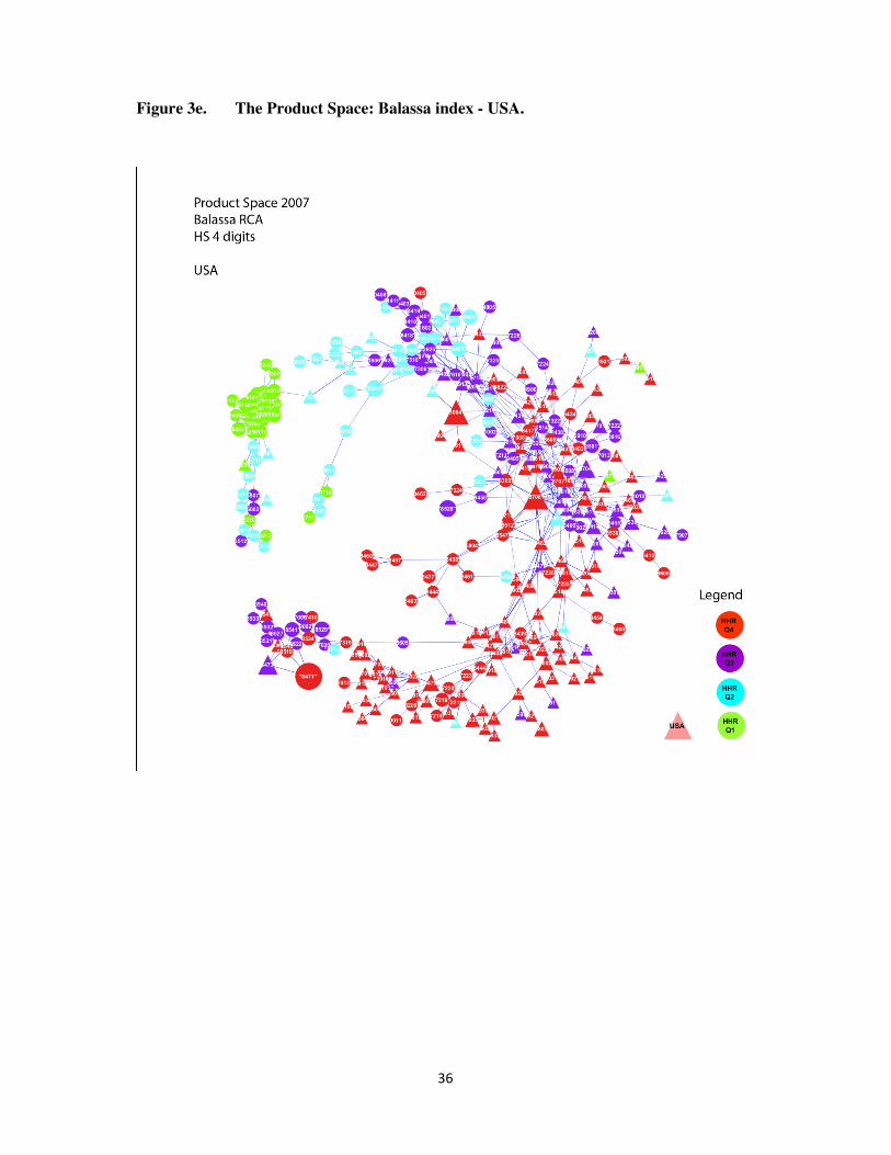
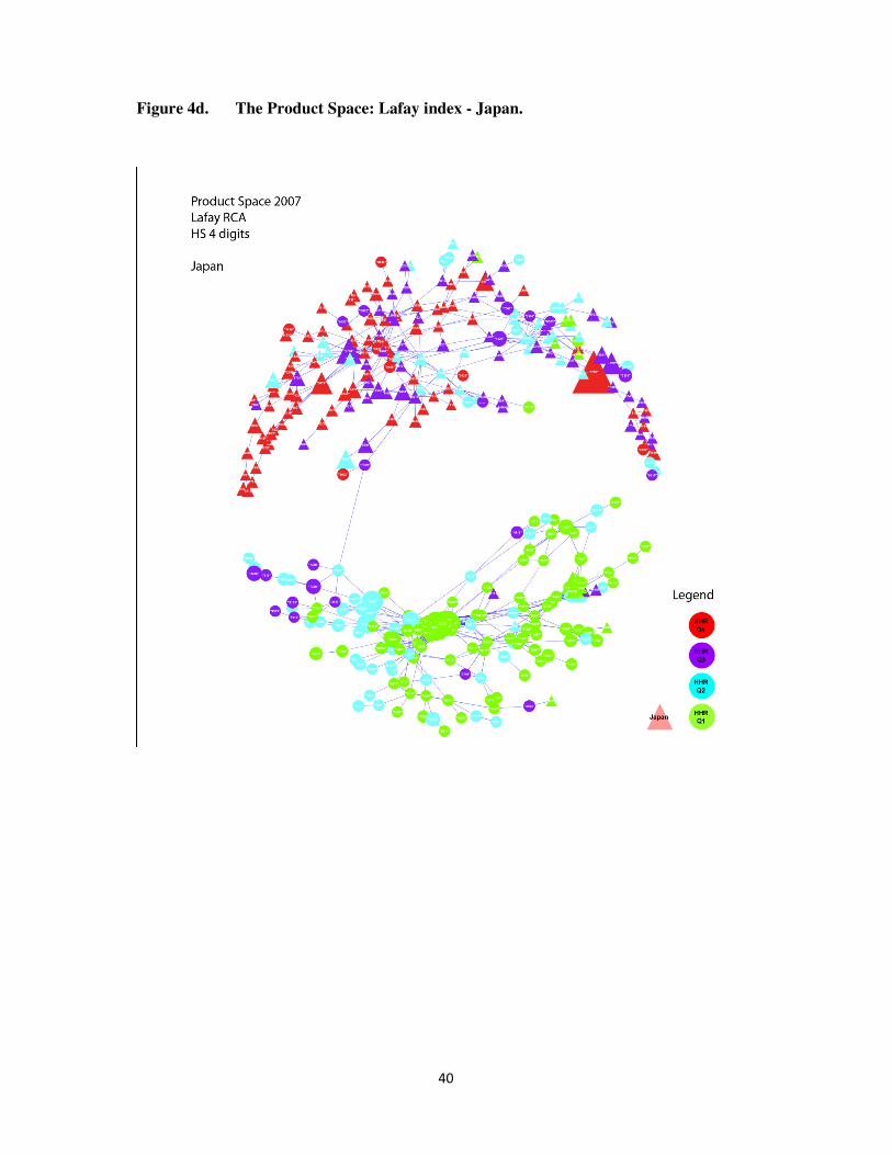
Pairwise proximities across all products form the basis for the analysis of the product

space. The methodology developed by Hidalgo and Hausmann (2007) makes use of network

analysis to illustrate the interactions between production sectors. To visualize the product

space, these proximities are read into Cytoscape (Shannon et al., 2003), an open source

platform for complex-network analysis and visualization, which applies a greedy algorithm

(spring-embedded) to cluster nodes along the intensity of the edges (proximities). To

facilitate visualization, we drop proximities smaller than 0.60. To categorize products, we

divide the distribution of PRODY into 4 classes, taking quartiles as delimiters (percentiles no.

25, 50, and 75). Graphically, categories 1 to 4 are associated to a different colour of the node

(products). Category 1 are low-GDPpc products (green), category 4 are highest-GDPpc

products (in red). Category 2 takes colour light-blue, category 3 is in dark blue. The size of

the nodes is determined by the share of products in total world trade.

11

The Balassa graphs (Figures 3a-3e) and Lafay graphs (Figures 4a-4e) look remarkably

different. The Balassa product space looks much more connected, whereas the Lafay product

space is almost dichotomized into two halves, with only one link between them with a

proximity index greater than 0.6 (the link is between sector 7309 - Tanks etc., over 300 Liter

Capacity, Iron or Steel, and sector 9406 - Prefabricated Buildings). In the Balassa product

space, products are ordered according to increasing values of PRODY in a clockwise fashion

starting from the top-left corner of the graph. In the Lafay space, low and middle-low

PRODY products are located in the lower half of the graph (from the right to the left), and

middle-high and high PRODY sectors in the top half (again right to left). If one considers net

trade flows as measures of capabilities as opposite to single-trade export flows only, thus, it

can be much more difficult to adapt and move to far away regions of the product space. In

particular, it can prove problematic to move from the two bottom quartiles of the PRODY

distribution to the two top quartiles.

According to the Balassa representation of the product space, China is over-

represented in the lowest quartiles of the PRODY distribution (Figure 3a). According to both

the Balassa and the Lafay graphs, however, China is also present in the third quartile of the

PRODY distribution. In particular, according to the Lafay index China has successfully

crossed the bridge to the upper half of the product space (Figure 4a). The potential

development prospects for China therefore look even brighter if we measure its specialization

in terms of net trade flows instead of single-trade flows.

According to both the Balassa and the Lafay metric, Germany is mostly represented in

the upper quartiles of the product space (Figures 3b and 4b). The same is true for Japan

(Figures 3d and 4d) and for the USA (Figures 3e and 4e).

The interpretation of the product space for India is quite complex. According to the

Balassa index, India is mostly present in the first and in the third quartiles of the PRODY

distribution, although it is also located in a number of products in the highest quartile (Figure

3c). According to the Lafay index, however, India is still over-represented in the lowest

quartile of the PRODY distribution, but it also has a strong presence in all the upper quartiles

of the productivity distribution, and has already established a specialization profile in the top

half of the product space (Figure 4c).

12

5. Trade specialization in China

China is as interesting case study for the purposes of the comparison between the Balassa and

the Lafay measures of comparative advantage, because the differences between total exports

and net exports can be quite significant in a number of sectors. From the discussion of the

product space in section 4, China occupies a somewhat higher productivity region of the

space according to the Lafay index compared to the Balassa index. Hence, its growth

prospects look even more encouraging if one looks at net trade flows.

Tables 5a and 5b list the top 25 and the bottom 25 ranking products for China at 6

digits according to the Balassa index, and Tables 6a and 6b list the corresponding products

according to the Lafay index. From Table 5a, it is apparent that some products that enjoy a

very high ranking according to the export specialization perform very poorly once we control

for net trade. In particular, product 282738 (Chlorides, Chloride Oxides And Hydroxide) is

ranked second according to Balassa, but only 3,053rd

according to Lafay. Similarly, item

293729 (Adrenal Cortical Hormones And Derivatives) is ranked 15th

according to Balassa but

only 2,954th

according to Lafay, item 1839 (Camphor) is ranked 16th

according to Balassa

and 1,839th

according to Lafay, and item 050210 (Pigs', hogs' or boars' bristles and hair and

waste thereof) is ranked 24th

and 1,074 respectively. By contrast, the lowest-ranking items

with the Balassa index also tend to have a low ranking according to Lafay (Figure 5b).

A similar pattern emerges if one looks at the top products according to the Lafay

index (Figure 6a). Item 852812 (TV Receivers, Color, Incl Video Monitors) is ranked 8th

and

1,540 according to Lafay and Balassa, item 847150 (Digital Processing Units) is ranked 16th

and 1,243rd

, item 844390 (Parts, of Printing Machinery, of Machines for Uses Ancillary to

Printing) is ranked 22nd

and 1,297th

, and item 890190 (Other vessels for the transport of

goods and other vessels for the transport of both persons and goods) is ranked 25th

and

1,759th

respectively. Again, no big surprises emerge from the products at the bottom of the

Lafay ranking.

In the case of China, therefore, one can reach quite different conclusions about the

pattern of product specialization if one uses net export flows rather than data on total exports.

The divergence between the two measures is also evident from Table 7, where the

values of the Open Forest indicator (equation (6)) are given. Open Forest is the average

PRODY of those products China is not present yet but are attainable (i.e. the distance-

13

weighted PRODY of all products that China is currently not producing but which it has the

potential to produce). This measure is much higher for the Balassa-based product space than

for that of Lafay. This may be reflective of China being already in a higher segment of the

product space according to Lafay, in line with the graphs in Figures 3a and 4a. The choice of

Lafay over Balassa is thus shown to have a strong bearing on the definition of product space.

6. Conclusions

This paper extends the analysis of the product space in two dimensions. It considers net trade

flows instead of single-trade flows as the basis for the measurement of comparative

advantage, and incorporates vertical specialization into the analysis. Both these extensions

are seen to be important in order to capture some aspects of the global pattern of trade

specialisation. The representation of the product space appears very different according to a

net-trade flow indicator compared to a single-trade flow indicator, with much fewer links to

connect low and medium-low productivity sectors to medium-high and high sectors.

Vertical specialization is analysed through the distribution of unit values within

sectors. When the proximity between sectors are combined with unit values and with the

Hausmann-Hwang-Rodrik index of productivity the pattern of trade specialization is radically

different for low and for high unit values, thus justifying a separate analysis along different

segments of the unit value distribution.

Ongoing research efforts expand the analysis on the basis of methods that better

capture the extent of production sharing and network trade. Revealed comparative indicators

reliant on net trade flows capture only in part the phenomenon of production fragmentation,

to the extent that such activities take place within the product categories and the degree of

aggregation chosen as the relevant level of analysis. By contrast, the explicit distinction of

trade in parts and components from trade in final goods, as reflected in the international trade

data, will provide a more reliable basis for the assessment of countries’ net capabilities.

14

Data Appendix

Trade data are drawn from the BACI dataset by the Centre d'Etudes Prospectives et

d'Informations Internationales(CEPII).5 Constructed on the basis of raw data from UN

Comtrade, the BACI dataset offers the advantage of broad coverage of trade flows measured

in volume, obtained through mirroring techniques of trade flow data available from UN

Comtrade partner countries' records. Therefore, the BACI dataset is particularly suitable for

the analysis of unit value data, which is one purpose of this paper's expansion of the unit

values concept. The data are disaggregated to six digits of the Harmonized System. For the

analysis, we use data alternatively at 6 and 4 digits of aggregation.

Population and GDP per capita series in purchasing power parity are obtained from the World

Bank's World Development Indicators (WDI), accessed online in August 2010. Data for

Taipei, China, where added from official country statistics, since missing in World Bank

statistics. To reduce possible noise deriving from the inclusion of very small, countries with

populations totaling less than 1 million were dropped from the database prior to computations.

Data availability in the BACI HS1996 database spans from 1998 to 2007.6 For this analysis,

we used the datasheet for the year 2007 only, leaving the analysis of the historical evolution

of the product space for future analysis.

5 For a description of the dataset, see http://www.cepii.fr/anglaisgraph/workpap/pdf/2010/wp2010-23.pdf

6 There is another version of BACI, HS1992, available for analysis, according to a previous nomenclature of HS

and spanning from 1995 to 2009.

15

Table 1. Trade specialization indicators: Balassa index (HS4).

Unit Values PRODY Country

Low High Q1 Q2 Q3 Q4

Whole

sample

China 2.74 1.79 2.60 3.02 2.47 1.62 2.56

Germany 1.82 1.88 1.13 1.59 2.02 2.21 1.86

India 3.74 3.99 6.69 3.07 2.67 1.54 3.81

Japan 1.65 1.40 0.59 1.02 1.73 1.89 1.46

USA 1.80 1.80 1.45 1.79 1.77 2.02 1.80

All Countries 6.61 5.11 17.31 3.10 1.90 1.26 5.89

Note: PRODY is computed as in equation (2); Q1-Q4 denote the quartiles of the PRODY distribution.

16

Table 2a. Balassa vs. Lafay: Pearson and Spearman correlation coefficients

(HS 4 digits).

Unit Values PRODY

Low High Q1 Q2 Q3 Q4

Whole

sample

Pearson 0.1879 0.0834 0.2242 0.0754 0.1401 0.2349 0.1399

Spearman 0.5696 0.4810 0.6406 0.5522 0.4753 0.4165 0.5257

Table 2b. Spearman’s rank correlation coefficients (HS 4 digits).

Country Spearman’s ρρρρ

China 0.7028

Germany 0.6518

India 0.6315

Japan 0.6907

USA 0.7207

Table 2c. Spearman’s rank correlation coefficients (HS 6 digits).

Country Spearman’s ρρρρ

China 0.6947

Germany 0.6175

India 0.6239

Japan 0.7037

USA 0.7073

17

Table 3a. Average proximities according to first digit of HS96 (4 digits).

First-digit product code

0 1 2 3 4 5 6 7 8 9

0 0.22 0.21 0.20 0.20 0.24 0.20 0.26 0.23 0.23 0.22

1 0.20 0.20 0.20 0.24 0.21 0.26 0.24 0.23 0.23

2 0.20 0.20 0.25 0.22 0.26 0.26 0.25 0.24

3 0.20 0.25 0.22 0.26 0.25 0.24 0.24

4 0.23 0.20 0.23 0.22 0.23 0.24

5 0.19 0.20 0.19 0.23 0.25

6 0.23 0.21 0.23 0.23

7 0.20 0.23 0.24

8 0.22 0.22

9 0.20

Table 3b. Average proximities according to first digit of HS96 (6 digits).

First-digit product code

0 1 2 3 4 5 6 7 8 9

0 0.19 0.19 0.19 0.22 0.23 0.20 0.26 0.22 0.22 0.21

1 0.21 0.19 0.23 0.24 0.21 0.26 0.23 0.23 0.22

2 0.18 0.23 0.26 0.24 0.27 0.26 0.26 0.25

3 0.21 0.22 0.22 0.27 0.24 0.25 0.23

4 0.21 0.20 0.26 0.23 0.24 0.22

5 0.22 0.27 0.26 0.26 0.25

6 0.24 0.21 0.23 0.22

7 0.22 0.25 0.24

8 0.23 0.22

9 0.19

18

Table 4a. Average proximity according to Unit Values and to the absolute

difference between PRODY quartiles (4 digits).

Unit Values Absolute difference between

PRODY quartiles HH HL LL

0 0.26 0.22 0.25

1 0.25 0.22 0.24

2 0.24 0.21 0.22

3 0.23 0.19 0.19

Table 4b. Average proximity according to Unit Values and to the absolute

difference between PRODY quartiles (6 digits).

Unit Values Absolute difference between

PRODY quartiles HH HL LL

0 0.26 0.23 0.27

1 0.26 0.22 0.26

2 0.25 0.21 0.24

3 0.22 0.19 0.21

19

Table 5a. China: Top ranking products according to the Balassa index.

Balassa

ranking

Lafay

ranking

Product code

(HS6)

Product name Balassa PRODY

1 760 580134 Woven Pile Fabrics Of Manmade

Fibers, Un..

8.90 7982

2 3053 282738 Chlorides, Chloride Oxides And

Hydroxide..

8.73 6316

3 190 940530 Magnetic Tapes For Sound

Recording Or Si..

8.60 13304

4 274 360410 Fireworks 8.32 15127

5 290 851672 Electrothermic Domestic

Appliances, N.E.S.

8.26 18879

6 509 610323 Ensembles, Of Knitted Or Crocheted

Texti..

8.01 7295

7 285 670420 Wigs, False Beards, Eyebrows,

Eyelashes,..

7.93 9561

8 480 500200 Raw Silk (Not Thrown) 7.86 2509

9 266 660199 Umbrellas And Sun Umbrellas

(Including W..

7.81 14245

10 39 950510 Articles, N.E.S. For Christmas

Festivities

7.80 12085

11 463 660191 Umbrellas And Sun Umbrellas

(Including W..

7.70 24452

12 336 670210 Artificial Flowers, Foliage Or Fruit

And..

7.70 18579

13 150 847010 Electronic Calculators Capable Of

Operat..

7.68 17268

14 605 280530 Calcium, Strontium And Barium;

Rare Eart..

7.64 24107

15 2954 293729 Adrenal Cortical Hormones And

Derivatives

7.63 13442

16 1839 291421 Camphor 7.46 10684

17 793 720280 Ferroalloys, N.E.S 7.43 15189

18 896 580123 Cotton Pile And Chenille Woven

Fabrics, ..

7.42 13873

19 462 940430 Sleeping Bags 7.42 8460

20 635 442110 Manufactured Articles Of Wood,

N.E.S.

7.32 17253

21 637 460120 Mats, Matting And Screens Of

Vegetable M..

7.32 3415

22 37 420212 Trunks, Suitcases, Vanity Cases,

Executi..

7.25 8230

23 118 392640 Articles Of Plastics, N.E.S. 7.20 13160

24 1074 050210 Pigs', hogs' or boars' bristles and hair 7.19 17049

25 72 841451 Fans, Table, Floor, Wall, Window,

Ceilin..

7.19 12480

20

Table 5b. China: Bottom ranking products according to the Balassa index.

Balassa

ranking

Lafay

ranking

Product code

(HS6)

Product name Balassa PRODY

5015 3881 040620 Grated Or Powdered Cheese, Of All

Kinds

0.00 25960

5016 3040 310280 Fertilizers, Urea And Ammonium

Nitrate M..

0.00 13489

5017 3111 030222 Flat Fish, Fresh Or Chilled

(Excluding L..

0.00 32649

5018 4768 261690 Ores And Concentrates Of Precious

Metals..

0.00 3049

5019 4240 151211 Sunflower Seed Oil Or Safflower

Oil, Crude

0.00 6381

5020 3482 051110 Bovine Semen 0.00 11833

5021 5040 290250 Styrene 0.00 31747

5022 3106 030231 Tunas, Skipjack Or Stripe 0.00 6103

5023 3731 120911 Sugar Beet Seed 0.00 20542

5024 4843 120500 Rape Or Colza Seeds 0.00 14023

5025 4997 260400 Nickel Ores And Concentrates 0.00 4432

5026 3358 030219 Salmonidae, Fresh Or Chilled

(Excluding ..

0.00 5446

5027 4936 711031 Platinum Group (Except Platinum)

Metals ..

0.00 12205

5028 3616 120924 Seeds Of Forage Plants, Other Than

Beet ..

0.00 33161

5029 3282 010111 Horses, Live 0.00 32267

5030 3423 410320 Hides And Skins, N.E.S., Raw

(Fresh, Sal..

0.00 2502

5031 3469 080121 Brazil Nuts, Fresh Or Dried,

Whether Or ..

0.00 5126

5032 5010 260800 Zinc Ores And Concentrates 0.00 6618

5033 4012 040690 Cheese, N.E.S. 0.00 18295

5034 3168 040640 Blue 0.00 32035

5035 5027 260112 Iron Ore Agglomerates (Sinters,

Pellets,..

0.00 10960

5036 4663 284410 Natural Uranium And Its

Compounds; Urani..

0.00 1211

5037 4468 180100 Cocoa Beans, Whole Or Broken,

Raw Or Roa..

0.00 1701

5038 4591 261210 Uranium Ores And Concentrates 0.00 1822

5039 3122 020726 Poultry Cuts (Of Chickens, Ducks,

Geese,..

0.00 20806

21

Table 6a. China: Top ranking products according to the Lafay index.

Lafay

ranking

Balassa

ranking

Product code

(HS6)

Product name Lafay PRODY

1 125 847130 Digital Processing Units Whether Or

Not P..

1.69 20399

2 651 852520 Transmission Apparatus For

Radiotelephon..

1.46 20532

3 665 847330 Parts Of Automatic Data Processing

Machi..

0.87 18665

4 242 847160 Input Or Output Units Whether Or

Not Pre..

0.56 19004

5 403 844359 Printing Machinery, N.E.S 0.50 17950

6 777 851780 Telephonic Or Telegraphic Apparatus,

N.E..

0.46 22439

7 49 950410 Video Games Of A Kind Used With

A Televi..

0.41 19870

8 1540 852812 TV Receivers, Color, Incl Video

Monitors..

0.40 16609

9 573 852540 Video Recording Or Reproducing

Apparatus..

0.36 17717

10 491 640399 Footwear, N.E.S., With Outer Soles

Of Le..

0.33 7810

11 200 950390 Toys, N.E.S. 0.33 19460

12 35 640299 Footwear, N.E.S., With Outer Soles

And U..

0.31 6640

13 141 852190 Video Recording Or Reproducing

Apparatus..

0.30 15970

14 517 850440 Static Converters (E.G., Rectifiers) 0.29 18566

15 161 950490 Articles For Funfair, Table And Parlor

G..

0.26 20261

16 1243 847150 Digital Processing Units Whether Or

Not P..

0.25 26930

17 598 611020 Jerseys, Pullovers, Cardigans,

Waistcoat..

0.24 3778

18 959 852990 Parts Of Television Receivers,

Radiobroa..

0.22 19955

19 608 620462 Trousers, Bib And Brace Overalls,

Breech..

0.22 4874

20 333 852821 TV Receivers, Color, Incl Video

Monitors..

0.21 19297

21 371 611030 Jerseys, Pullovers, Cardigans,

Waistcoat..

0.21 4713

22 1297 844390 Parts For Printing Machinery And

Parts O..

0.19 22582

23 505 853400 Printed Circuits 0.19 20836

24 145 851999 Sound Reproducing Apparatus, N.E.S. 0.18 22157

25 1759 890190 Vessels For The Transport Of Goods

(Incl..

0.18 7447

22

Table 6b. China: Bottom ranking products according to the Lafay index.

Lafay

ranking

Balassa

ranking

Product code

(HS6)

Product name Lafay PRODY

5030 4650 390120 Polyethylene, Having A Specific

Gravity ..

-0.15 21817

5031 4393 870840 Gear Boxes -0.16 23737

5032 4227 750210 Nickel, Unwrought (Not Alloyed) -0.17 16513

5033 4144 390330 Acrylonitrile -0.18 24144

5034 4950 854250 Electronic Integrated Circuits And

Micro..

-0.18 3246

5035 4581 390210 Polypropylene, In Primary Forms -0.19 19265

5036 4951 151190 Palm Oil, Refined, And Its Fractions -0.19 6990

5037 3714 290243 Xylenes, Pure -0.19 21017

5038 4739 520100 Cotton (Other Than Linters), Not

Carded ..

-0.21 1681

5039 4655 870323 Motor Vehicles For The Transport Of

Pers..

-0.22 19257

5040 5021 290250 Styrene -0.25 31747

5041 4826 290531 Ethylene Glycol (Ethanediol) -0.27 27530

5042 5013 291736 Polycarboxylic Acids, N.E.S. And

Their A..

-0.35 18297

5043 5000 870324 Motor Vehicles For The Transport Of

Pers..

-0.37 28396

5044 4185 740400 3936er Waste And Scrap -0.41 7785

5045 3783 847989 Machinery Having Individual

Functions, N..

-0.51 26716

5046 4943 260300 Copper Ores And Concentrates -0.51 5146

5047 4340 120100 Soybeans -0.60 6793

5048 4263 740311 Refined Copper -0.60 4897

5049 4119 271000 line Including Aviation (Except Jet)

Fuel

-0.66 14760

5050 4651 880240 Airplanes And Other Aircraft,

Mechanical..

-0.67 23639

5051 4884 260111 Iron Ore And Concentrates, Not

Agglomera..

-1.16 7501

5052 1592 901380 Liquid Crystal Devices, N.E.S. And

Optic..

-1.20 26519

5053 2716 854230 Nondigital Monolithic Integrated

Units

-3.27 23293

5054 4815 270900 Petroleum Oils And Oils From

Bituminous ..

-4.31 12115

23

Table 7. China: Density and Open Forest indices.

Density Open forest

Balassa Lafay Balassa Lafay

mean 0.53 0.67 7.90e+06 2.06e+06

median 0.51 0.66 7.90e+06 2.06e+06

SD 0.12 0.08 0.00 0.00

min 0.13 0.45 7.90e+06 2.06e+06

max 0.96 1.00 7.90e+06 2.06e+06

24

Figure 1a. PRODY and Cumulated Lafay Index, HS 4 digits – China.

-20

24

68

01

00

00

200

00

300

00

400

00

GDPpc USD (left) Cumulated Lafay Index (right)

China - HS4

Figure 1b. PRODY and Cumulated Lafay Index, HS 4 digits – Germany.

-8-6

-4-2

0

01

00

00

200

00

300

00

400

00

GDPpc USD (left) Cumulated Lafay Index (right)

Germany - HS4

25

Figure 1c. PRODY and Cumulated Lafay Index, HS 4 digits – India.

05

10

15

01

00

00

200

00

300

00

400

00

GDPpc USD (left) Cumulated Lafay Index (right)

India - HS4

Figure 1d. PRODY and Cumulated Lafay Index, HS 4 digits – Japan.

-20

-15

-10

-50

01

00

00

200

00

300

00

400

00

GDPpc USD (left) Cumulated Lafay Index (right)

Japan - HS4

26

Figure 1e. PRODY and Cumulated Lafay Index, HS 4 digits – USA.

-10

-8-6

-4-2

0

01

00

00

200

00

300

00

400

00

GDPpc USD (left) Cumulated Lafay Index (right)

USA - HS4

27

Figure 2a(i). PRODY and Cumulated Lafay Index, HS 4 digits, Low Unit Values –

China.

05

10

15

20

01

00

00

200

00

300

00

400

00

GDPpc USD (left) Cumulated Lafay Index (right)

China - HS4 - Low UVs

Figure 2a(ii). PRODY and Cumulated Lafay Index, HS 4 digits, High Unit Values –

China.

-20

-15

-10

-50

01

00

00

200

00

300

00

400

00

GDPpc USD (left) Cumulated Lafay Index (right)

China - HS4 - High UVs

28

Figure 2b(i). PRODY and Cumulated Lafay Index, HS 4 digits, Low Unit Values –

Germany.

-6-4

-20

01

00

00

20

00

03

00

00

40

00

0

GDPpc USD (left) Cumulated Lafay Index (right)

Germany - HS4 - Low UVs

Figure 2b(ii). PRODY and Cumulated Lafay Index, HS 4 digits, High Unit Values –

Germany.

-50

5

01

00

00

200

00

300

00

400

00

GDPpc USD (left) Cumulated Lafay Index (right)

Germany - HS4 - High UVs

29

Figure 2c(i). PRODY and Cumulated Lafay Index, HS 4 digits, Low Unit Values –

India.

05

10

01

00

00

200

00

300

00

400

00

GDPpc USD (left) Cumulated Lafay Index (right)

India - HS4 - Low UVs

Figure 2c(ii). PRODY and Cumulated Lafay Index, HS 4 digits, High Unit Values –

India.

-10

-50

5

01

00

00

200

00

300

00

400

00

GDPpc USD (left) Cumulated Lafay Index (right)

India - HS4 - High UVs

30

Figure 2d(i). PRODY and Cumulated Lafay Index, HS 4 digits, Low Unit Values –

Japan.

-8-6

-4-2

0

01

00

00

200

00

300

00

400

00

GDPpc USD (left) Cumulated Lafay Index (right)

Japan - HS4 - Low UVs

Figure 2d(ii). PRODY and Cumulated Lafay Index, HS 4 digits, High Unit Values –

Japan.

-15

-10

-50

5

01

00

00

200

00

300

00

400

00

GDPpc USD (left) Cumulated Lafay Index (right)

Japan - HS4 - High UVs

31

Figure 2e(i). PRODY and Cumulated Lafay Index, HS 4 digits, Low Unit Values – USA.

-15

-10

-50

01

00

00

200

00

300

00

400

00

GDPpc USD (left) Cumulated Lafay Index (right)

USA - HS4 - Low UVs

Figure 2e(ii). PRODY and Cumulated Lafay Index, HS 4 digits, High Unit Values –

USA.

-50

51

01

5

01

00

00

200

00

300

00

400

00

GDPpc USD (left) Cumulated Lafay Index (right)

USA - HS4 - High UVs

32

Figure 3a. The Product Space: Balassa index - China.

33

Figure 3b. The Product Space: Balassa index - Germany.

34

Figure 3c. The Product Space: Balassa index - India.

35

Figure 3d. The Product Space: Balassa index - Japan.

36

Figure 3e. The Product Space: Balassa index - USA.

37

Figure 4a. The Product Space: Lafay index - China.

38

Figure 4b. The Product Space: Lafay index - Germany.

39

Figure 4c. The Product Space: Lafay index - India.

40

Figure 4d. The Product Space: Lafay index - Japan.

41

Figure 4e. The Product Space: Lafay index - USA.

42

References

Alessandrini, M., B. Fattouh, B. Ferrarini and P. Scaramozzino (2009), “Tariff Liberalization

and Trade Specialization in India”, Asian Development Bank, ADB Economics, Working

Paper No. 177, November.

Athukorala, P.-C., and J. Menon (2010), “Global Production Sharing, Trade Patterns, and

Determinants of Trade Flows in East Asia”, Asian Development Bank, ADB Working Paper

Series on Regional Economic Integration No. 41, January.

Balassa, B. (1986), “Comparative Advantage in Manufactured Goods: A Reappraisal”,

Review of Economics and Statistics, Vol. 68, No. 2, May, pp. 315-319.

Brülhart, M. (2008), “An Account of Global Intra-industry Trade, 1962-2006”, GEP

Leverhulme Centre, University of Nottingham, Research Paper 2008/08.

Bugamelli, M. (2001), “Il Modello di Specializzazione Internazionale dell’Area dell’Euro e

dei Principali Paesi Europei: Omogeneità e Convergenza”, Temi di Discussione 402, Banca

d’Italia, Rome.

Fontagné, L., M. Freudenberg and G. Gaulier (2006), “A Systematic Decomposition of

World Trade into Horizontal and Vertical IIT”, Review of World Economics, Vol. 142, No. 3,

pp. 459-475.

Gaulier, G., and S. Zignago (2010), “BACI: International Trade Database at the Product-level.

The 1994-2007 Version”, CEPII, Centre d’Etudes Prospectives et d’Informations

Internationales”, Working Paper No. 2010-23, October.

Greenaway, D., and C. R. Milner (2003), “What Have We Learned from a Generation’s

Research on Intra-Industry Trade?”, GEP Leverhulme Centre, University of Nottingham,

Research Paper 2003/44.

Greenaway, D., and J. Torstensson (1997), “Back to the Future: Taking Stock on Intra-

Industry Trade”, Weltwirtschaftiches Archiv, Vol. 133, No. 2, pp. 249-269.

Hausmann, R., J. Hwang and D. Rodrik (2007), “What You Export Matters”, Journal of

Economic Growth, Vol. 12, pp. 1-25.

Hausmann, R., and B. Klinger (2006), “Structural Transformation and Patterns of

Comparative Advantage in the Product Space”, Centre for International Development,

Harvard University, Working Paper No. 128.

Hausmann, R., and B. Klinger (2007), “The Structure of the Product Space and the Evolution

of Comparative Advantage”, Centre for International Development, Harvard University,

Working Paper No. 146.

Hidalgo, C. A. (2009), “The Dynamics of Economic Complexity and the Product Space over

a 42 Year Period”, Centre for International Development, Harvard University, Working Paper

No. 189.

43

Hidalgo, C. A., and R. Hausmann (2009), “The Building Blocks of Economic Complexity”,

Proceedings of the National Academy of Sciences, Vol. 106, No. 26, June 30, pp. 10570-

10575.

Hidalgo, C. A., B. Klinger, A.-L. Barabási, and R. Hausmann (2007), “The Product Space

Conditions the Development of Nations”, Science, Vol. 317, 27 July, pp. 482-487.

Hirschman, A. (1958), The Strategy of Economic Development, New Haven, Conn., Yale

University Press.

Iapadre, P. L. (2001), “Measuring International Specialization”, International Advances in

Economic Research, Vol. 7, No. 2, May.

Lafay, G. (1992), “The Measurement of Revealed Comparative Advantage”, in M. G.

Dagenais and P. A. Muet (eds), International Trade Modelling, London, Chapman & Hall.

Schott, P. K. (2004), “Across-Product versus Within-Product Specialization in International

Trade”, Quarterly Journal of Economics, Vol. 119, No. 2, May, pp. 647-678.

Shaked, A., and J. Sutton (1984), “Natural Oligopolies and International Trade”, in H.

Kierzkowski (ed.), Monopolistic Competition and International Trade, Oxford, Oxford

University Press.

Shannon P., A. Markiel, O. Ozier, N.S. Baliga, J.T. Wang, D. Ramage, N. Amin, B.

Schwikowski and T. Ideker (2003), “Cytoscape: A Software Environment for Integrated

Models of Biomolecular Interaction Networks”, Genome Research, Vol. 13, No. 11,

November, pp. 2498-2504.

Sutton, J. (1986), “Vertical Product Differentiation: Some Basic Themes”, American

Economic Review, Vol. 76, No. 2, Papers and Proceedings, May, pp. 393-398.

Sutton, J. (2001), “Rich Trades, Scarce Capabilities: Industrial Development Re-visited”,

Keynes Lecture, British Academy, 2000, Proceedings of the British Academy 2001.

Zaghini, A. (2005), “Evolution of Trade Patterns in the New EU Member States”, Economics

of Transition, 13(4), 629-658.