Indiana University-Purdue University Fort Wayne ECE 406 ...

Indiana University-Purdue University Fort Wayne Department of Electrical and Computer Engineering

ECE 406

Senior Engineering Design II

Final Report

Project Title: Use of Stereoscopic Imaging for Distance Determination

Team Members: Andrew Fullenkamp

Christopher Nei Kaleb Krempel

Faculty Advisor: Elizabeth Thompson, Ph.D. Advisor: Timothy Loos, Ph.D.

Date: 4/19/2016

P a g e | 1

Contents Acknowledgements .................................................................................................................... 4

Abstract/Summary ..................................................................................................................... 5

Section I: Problem Statement ..................................................................................................... 7

Introduction ............................................................................................................................ 7

Requirements and Specifications ........................................................................................... 7

Given Parameters or Quantities.............................................................................................. 7

Design Variables .................................................................................................................... 7

Limitation and Constraints ...................................................................................................... 7

Section II: Conceptual Designs .................................................................................................. 8

Camera Hardware .................................................................................................................. 8

Type 1: Digital Single Lens Reflex (DSLR) Cameras .......................................................... 8

Type 2: Point-And-Shoot Cameras...................................................................................... 8

Type 3: Web Cameras. ....................................................................................................... 8

Type 4: Prefabricated stereo camera. ................................................................................. 9

Image Processing Unit ........................................................................................................... 9

Option 1: Implement on a Raspberry Pi (RPi). .................................................................... 9

Option 2: Use an alternative micro-computer system. ........................................................10

Option 2a: Hummingboard .................................................................................................11

Option 2b: ASUS VivoMini .................................................................................................12

Option 3: Relay image data to a deployable PC application. ..............................................13

GUI for System Management (for embedded image processing platforms) ...........................14

Option 1: Connect a screen to the Image Processing Unit: ................................................14

Option 2: Run a web server on the Image Processing Unit: ...............................................14

Conceptual Designs ..............................................................................................................14

Design 1: A Simplified Approach. .......................................................................................14

Designs 2: Virtual Stereo Using Translational Camera .......................................................15

Design 3: Virtual Stereo Using an Array of Mirrors .............................................................16

Design 4: Implementation of Image Processing Application Option 3 .................................17

Section III: Summary of the Evaluation of the Conceptual Designs ...........................................19

Camera Type Selection .........................................................................................................19

System Configuration Selection .............................................................................................21

Section IV: A Detailed Design of the Selected Conceptual Design ............................................24

Theoretical Considerations ....................................................................................................24

Hardware ...............................................................................................................................24

Image Processing ..................................................................................................................27

P a g e | 2

The User Interface .................................................................................................................29

Stereo Camera Calibration ....................................................................................................30

Section V: Design Implementation ............................................................................................33

Construction of the Apparatus ...............................................................................................33

Stereo Camera Alignment .....................................................................................................34

Calibrating Individual Cameras ..............................................................................................35

Calibrating the Overall System ..............................................................................................37

User Interface for System Control ..........................................................................................41

Accessing the User Interface .............................................................................................41

System Home ....................................................................................................................43

Camera Trigger ..................................................................................................................45

User Targeting ...................................................................................................................46

Results Plot ........................................................................................................................49

Section VI: Testing ....................................................................................................................51

Position Estimate Accuracy ...................................................................................................51

Repeatability Considerations .................................................................................................53

Lighting and White Balance Considerations ..........................................................................54

Section VII: Cost Analysis .........................................................................................................58

Recommendations ....................................................................................................................59

Conclusion ................................................................................................................................59

References ...............................................................................................................................60

Appendix A: Intrinsic Parameters for Stereo Cameras from Camera Calibration Procedure. .....61

Interpretation of Intrinsic Parameters .....................................................................................61

Intrinsic Parameters of Left Stereo Camera ...........................................................................61

Intrinsic Parameters of Right Stereo Camra ..........................................................................62

Appendix B: Raw Calibration Point Data ...................................................................................63

Appendix C: Source Code for System User Interface ................................................................68

/index.html .............................................................................................................................68

/interfaceStyles.css................................................................................................................70

/TargetCounts.php .................................................................................................................71

/cgi-bin/CameraInit.sh ............................................................................................................71

/cgi-bin/CameraTrigger.html ..................................................................................................72

/cgi-bin/CameraTrigger.sh .....................................................................................................72

/UserTargeting/index.html......................................................................................................73

/cgi-bin/ImportCSV.php .........................................................................................................82

/cgi-bin/ExportCSV.php .........................................................................................................83

P a g e | 3

/ResultsPlot/index.php ...........................................................................................................83

/ResultsPlot/CPointUndistort .................................................................................................86

P a g e | 4

Acknowledgements Many Individuals have been influential in the development of this project. We would like to thank those that have been kind enough to lend hardware for testing the concepts entailed in this document. Specifically, we thank Dr. Wang for his Raspberry Pi unit and Jeff Ballinger for his webcam. We would also like to thank our mechanical engineering colleagues Adam Fullenkamp and Jason Joyner for advising us on the design of our test stand. Lastly, we wish to express our sincere gratitude Dr. Elizabeth Thompson and Dr. Timothy Loos for advising us throughout the development of this project.

P a g e | 5

Abstract/Summary Stereo imaging, also referred to as binocular imaging, is a method of image capture wherein the same field of view is recorded by 2 camera units that are offset slightly from one another as shown in Figure 1.

Figure 1 (adapted from Jernej & Vrančić): This figure shows planar geometry of a visual system in which 2 cameras with angular fields of view, θ, and image resolutions of xo pixels are separated by the distance B and aligned in parallel to capture stereo images

of an object Z meters away. The values xl’ and xr’ denote the position of the object within the field imaged by each camera in this system.

The offset distance between the cameras in this configuration, also referred to as the stereo baseline distance (B), causes an individual object to appear at different coordinates within a pair of images taken by both cameras simultaneously. If these cameras lie on the same plane and are aligned in parallel as shown, then this position difference, also referred to as pixel disparity (d), exists only in the lateral dimension of such image sets. Provided this condition is met, the variables Z and d are related by the trigonometric relationship

(1)

(Jernej, & Vrančić). Alternatively, Figure 2 provides a more commonly used model for the geometry of parallel stereo vision systems that uses similar triangles to prove that

P a g e | 6

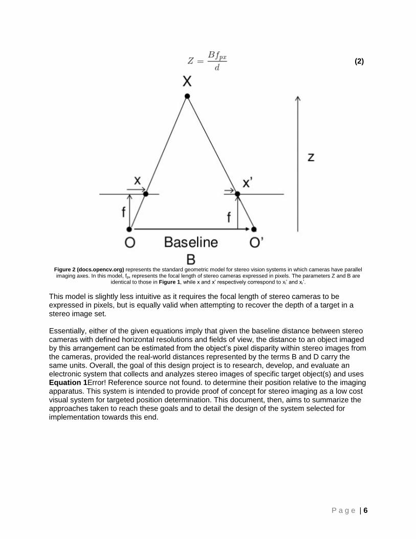
(2)

Figure 2 (docs.opencv.org) represents the standard geometric model for stereo vision systems in which cameras have parallel imaging axes. In this model, fpx represents the focal length of stereo cameras expressed in pixels. The parameters Z and B are

identical to those in Figure 1, while x and x’ respectively correspond to xl’ and xr’.

This model is slightly less intuitive as it requires the focal length of stereo cameras to be expressed in pixels, but is equally valid when attempting to recover the depth of a target in a stereo image set. Essentially, either of the given equations imply that given the baseline distance between stereo cameras with defined horizontal resolutions and fields of view, the distance to an object imaged by this arrangement can be estimated from the object’s pixel disparity within stereo images from the cameras, provided the real-world distances represented by the terms B and D carry the same units. Overall, the goal of this design project is to research, develop, and evaluate an electronic system that collects and analyzes stereo images of specific target object(s) and uses Equation 1Error! Reference source not found. to determine their position relative to the imaging apparatus. This system is intended to provide proof of concept for stereo imaging as a low cost visual system for targeted position determination. This document, then, aims to summarize the approaches taken to reach these goals and to detail the design of the system selected for implementation towards this end.

P a g e | 7

Section I: Problem Statement Introduction The goal of this design project is to research, develop, and evaluate an electronic system that captures binocular/stereo images of defined reference objects and uses the set to determine its position relative to them. In order to be considered a viable design solution, the system is expected to meet the main requirements, specifications, constraints, and directives delineated below. Requirements and Specifications

System will consist of a set of cameras for capturing stereo images connected to an image processing unit.

The arrangement should be able to determine the distance to a preset reference object up to 5 meters away with less than 6% error.

Image processing unit will need to identify reference objects common to stereo images and use offset information to calculate distances and locational information.

The time for a position calculation to complete after it is triggered should not exceed 6 seconds.

Apparatus must have a user Interface that guides the user through the processes of: o Setup - Directs the positioning of the cameras to capture a pair of images

containing target object(s). o Stereo image capture. o Displaying results of distance calculations. o Notifying the user about any errors that arise. o Advanced Setup - Camera interface settings/parameters. o Calibration – Process that adjusts distance calculation parameters based on

imaging system characteristics. Given Parameters or Quantities

Cost – System component costs should not exceed $300.

Testing Conditions: o Internal environment with standard office/industrial lighting.

Design Variables

Camera field of view and resolution must be balanced with a stereo baseline that optimizes distance calculations for objects within the specified range.

Reference/Target Object(s) – Object(s) with a defined color and size that are easily identified during image processing for distance calculation algorithms.

Limitation and Constraints

Apparatus will determine 2-dimensional position data. Reference objects should lie in the same plane as camera hardware.

Portability – System should be easily moved by an individual person o System should have a cumulative weight of less than 50 lb. o Cameras and fixture should occupy less than 2 m3.

Cameras should be commercially available, having specifications within typical ranges.

Computational resources (RAM, processor speed, etc.) available to the image processing unit.

P a g e | 8

Section II: Conceptual Designs It is beneficial to divide the proposed system into 3 sub-systems: the camera hardware responsible for image acquisition, an image processing unit for image analysis and position calculations, and a user interface program capable of managing the system’s operational processes. For each of these sub-systems, it is necessary to generate a set of component and approach options that can be compiled to form a system that is viable as a whole. The following text provides a brief description of design elements belonging to each set as well as some of the advantages and disadvantages they offer to the overall design.

Camera Hardware

Type 1: Digital Single Lens Reflex (DSLR) Cameras Pros:

Utilize high quality lenses with identified focal lengths and minimized lens distortion

Interchangeable lens allows for selectable angular field of view.

Several models support remote control via Picture Transfer Protocol (PTP) standard. Cons:

Difficulty finding two cameras of this type with matching lenses that are available within budget.

Models that are available within budget typically have lower resolutions than 8 MP.

Type 2: Point-And-Shoot Cameras Pros:

Allow for the high resolution photo capture offered by DLSR units at less cost.

Compact

Certain models support remote control via Picture Transfer Protocol (PTP) standard. Cons:

Small size of point-and-shoot units provides fewer attachment points for mounting

Type 3: Web Cameras. Pros:

Readily available at low cost.

Designed to work with computers, streamlining camera interfacing processes.

Cons:

The resolution of commercial products is generally lower compared to other alternatives, as they are designed for capturing video over still images.

P a g e | 9

Type 4: Prefabricated stereo camera.

Figure 3 shows a FujiFilm FinePix Real 3D W3 Digital Camera capable of capturing stereo images. Image obtained from

Amazon.com

Pros:

Stereo lenses are already constructed and aligned to work in tandem, simplifying system setup and calibration.

Cons:

Cost – Such units are commodity items and are therefore more expensive and less common in commercial markets.

Most pre-fabricated units have a set distance between stereo lenses intended to produce “3D” images. Greater camera separation is related to the accuracy of position determination, meaning this relatively small, fixed lens separation could prove limiting with regards to the accuracy of such calculations.

Image Processing Unit An image processing unit is necessary to analyze the stereo images obtained by the camera set to locate any target/reference objects contained therein. To do this, the unit will need to make use of some form of region of interest detection, several of which are available within MATLAB as well as the Open Computer Vision (OpenCV) libraries available to the C++, Java, and Python programming languages. The exact method(s) by which target recognition can be achieved are examined later in this document, but for the moment, some of the options for an image processing platform on which to implement this process will be examined.

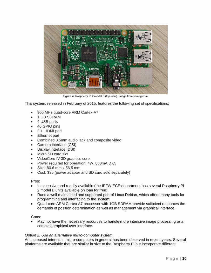
Option 1: Implement on a Raspberry Pi (RPi). Raspberry Pi is a series of low-profile single board computer systems intended for teaching lessons in basic computer science and hardware configuration. Within the past decade, this platform has accumulated a large support community of professional and independent developers alike due to its low cost and general applicability to the development of small-scale electronic/computational systems. The most recently released product in this series is the Raspberry Pi 2 Model B, depicted in Figure 4

P a g e | 10

Figure 4: Raspberry Pi 2 model B (top view). Image from pcmag.com.

This system, released in February of 2015, features the following set of specifications:

900 MHz quad-core ARM Cortex-A7

1 GB SDRAM

4 USB ports

40 GPIO pins

Full HDMI port

Ethernet port

Combined 3.5mm audio jack and composite video

Camera interface (CSI)

Display interface (DSI)

Micro SD card slot

VideoCore IV 3D graphics core

Power required for operation: 4W, 800mA D.C.

Size: 80.6 mm x 56.5 mm

Cost: $35 (power adapter and SD card sold separately)

Pros:

Inexpensive and readily available (the IPFW ECE department has several Raspberry Pi 2 model B units available on loan for free).

Runs a well-maintained and supported port of Linux Debian, which offers many tools for programming and interfacing to the system.

Quad-core ARM Cortex A7 processor with 1GB SDRAM provide sufficient resources the demands of position determination as well as management via graphical interface.

Cons:

May not have the necessary resources to handle more intensive image processing or a complex graphical user interface.

Option 2: Use an alternative micro-computer system. An increased interest in micro-computers in general has been observed in recent years. Several platforms are available that are similar in size to the Raspberry Pi but incorporate different

P a g e | 11

processors, RAM, and periphery hardware. Two promising examples of such system are the HummingBoard and the ASUS VivoMini, which are described in more detail below.

Pros:

Superior hardware to a Raspberry Pi.

Cons:

More expensive than Raspberry Pi.

Alternative units are still embedded or low-end modular systems. Even with improved processing resources, they can still be overtaxed by the demands of complex algorithms and interfaces.

Option 2a: Hummingboard HummingBoard is a product line consisting of several ARM-based micro-computers intended to act as an interface to other electronic components within a modular system. As shown in Figure 5, HummingBoards, like Raspberry Pis, come in several configurations featuring, in general, USB, GPIO, HDMI, and Ethernet ports as well as an SD card slot.

Figure 5 shows the layout of a HummingBoard Gate, the least expensive HummingBoard system configuration. Image from solid-

run.com.

Unlike the RPi, however, each HummingBoard offers a set of SOM (System On Module) controller options. Each SOM contains the processor, RAM, network interface, and other periphery components that provide support for many common features of modern computer systems. Prominent features/specifications of HummingBoard products overall include:

1 GHz ARM Cortex A9 processors (single, dual, or quad core)

512 MB or 1-2 GB DDR3 RAM

2 USB Ports

P a g e | 12

10/100/1000 Mbps Ethernet (Optional WiFi)

Bluetooth v4.0 interface

Linux Support

mikroBUS (proprietary) interface for additional periphery modules.

Power required for operation: 10W, 2A D.C.

Size: 85 mm x 56mm or 102 mm x 69 mm (depending on configuration)

Cost: $50 - $250 (depending on configuration)

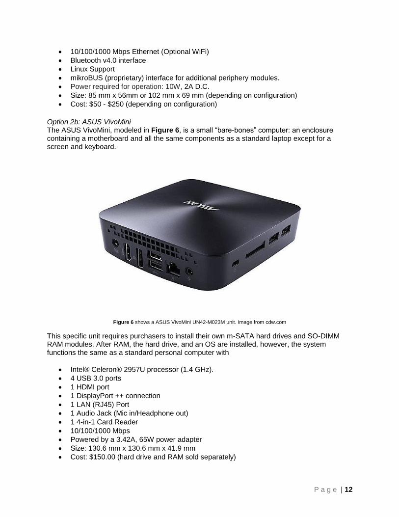
Option 2b: ASUS VivoMini The ASUS VivoMini, modeled in Figure 6, is a small “bare-bones” computer: an enclosure containing a motherboard and all the same components as a standard laptop except for a screen and keyboard.

Figure 6 shows a ASUS VivoMini UN42-M023M unit. Image from cdw.com

This specific unit requires purchasers to install their own m-SATA hard drives and SO-DIMM RAM modules. After RAM, the hard drive, and an OS are installed, however, the system functions the same as a standard personal computer with

Intel® Celeron® 2957U processor (1.4 GHz).

4 USB 3.0 ports

1 HDMI port

1 DisplayPort ++ connection

1 LAN (RJ45) Port

1 Audio Jack (Mic in/Headphone out)

1 4-in-1 Card Reader

10/100/1000 Mbps

Powered by a 3.42A, 65W power adapter

Size: 130.6 mm x 130.6 mm x 41.9 mm

Cost: $150.00 (hard drive and RAM sold separately)

P a g e | 13

Though not an embedded system, this unit offers all the benefits of using a full low-end computer as the image processor/user interface for a design while still retaining the small physical profile of an embedded system. Note that systems represent possible alternatives to the Raspberry Pi that could be implemented as the image processor for this system. Their inclusion in this document does not preclude the application of other commercial micro-computers that have comparable or superior costs/specifications. Also note that commercial units with superior hardware to the Raspberry Pi come at increased cost. Based on this, to be considered as a viable RPi alternative, a given system must meet or exceed the following qualifications (listed in order of descending importance), as is the case with the example platforms detailed above.

Must have support for USB camera interface.

CPU must have a clock frequency greater than 900 MHz

Must have greater than 512 MB of RAM

Must be capable of running applications written in standard C/C++, Java, and Python programming languages.

Should support a Linux operating system such as Lubuntu or Debian.

Must include a 100 Mbps or faster network interface.

Must be capable of hosting at least a minimal web server.

Option 3: Relay image data to a deployable PC application. In this system, a stand-alone computer application would be written that could communicate directly with the stereo cameras or, more likely, through a micro-computer such as a Raspberry Pi.

Pros:

Computers and laptops can handle processing that embedded alternatives cannot.

MATLAB could be used to handle image processing on the deploy system.

Interaction does not require the user to be within reach of the unit.

Cons:

Wireless communications between program and camera interface must be established.

Requires the sending of full images to the application, which could result in response delays during program interaction.

Requires development of 2 programs, one to be implemented on the deploy system, the other to run on the camera interface system to relay images to the former.

P a g e | 14

GUI for System Management (for embedded image processing platforms) For any implementation of this system as a whole, a graphical interface application must be developed that is responsible for managing.

Apparatus setup

The capture of stereo images

Displaying results of distance calculations.

Notifying the user about any errors that arise.

Advanced Setup (Camera interface settings & calibration).

Option 1: Connect a screen to the Image Processing Unit: Pros:

No wireless interfacing required. Everything is handled at the main interface location.

Cons:

Interaction requires the user to be within reach of the unit.

Requires the purchase of a compatible screen.

Option 2: Run a web server on the Image Processing Unit: Pros:

Interaction does not require the user to be within reach of the unit.

Interface is cross-platform, accessed via web browser.

Cons:

Requires wired and/or wireless networking.

Places additional demand on the image processing unit.

Conceptual Designs From the list of component design options given above, several design alternatives for the overall system given can be conceptualized. Note that the choice of camera hardware for the system is an important design decision. It is therefore assumed in the following conceptual designs that the effects of changing the camera type within a system are limited to the hardware level and the means by which the system controller interacts with cameras of that type. It is also assumed that each conceptual design does not depend on features exclusive to one specific controller unit. Provided this, should a chosen controller prove insufficient to handle the processing requirements for its associated system, it can be exchanged with another unit possessing more powerful computational hardware. Therefore, in each of the

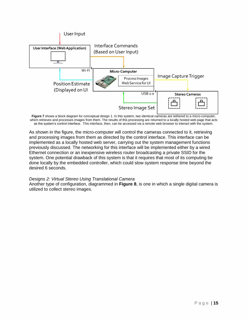
Design 1: A Simplified Approach. One mechanically simple approach to the given system is represented by the combination of sub-systems described above and shown in Figure 7.

P a g e | 15

Figure 7 shows a block diagram for conceptual design 1. In this system, two identical cameras are tethered to a micro-computer,

which retrieves and processes images from them. The results of this processing are returned to a locally hosted web page that acts as the system’s control interface. This interface, then, can be accessed via a remote web browser to interact with the system.

As shown in the figure, the micro-computer will control the cameras connected to it, retrieving and processing images from them as directed by the control interface. This interface can be implemented as a locally hosted web server, carrying out the system management functions previously discussed. The networking for this interface will be implemented either by a wired Ethernet connection or an inexpensive wireless router broadcasting a private SSID for the system. One potential drawback of this system is that it requires that most of its computing be done locally by the embedded controller, which could slow system response time beyond the desired 6 seconds.

Designs 2: Virtual Stereo Using Translational Camera Another type of configuration, diagrammed in Figure 8, is one in which a single digital camera is utilized to collect stereo images.

P a g e | 16

Figure 8 shows a block diagram for conceptual design 2. In this system, a single digital camera is translated between stereo

positions. This camera is tethered to a micro-computer, which retrieves the images it stores and processes them. The results of this processing are returned to a locally executed control interface, viewed on a screen connected to the micro-computer.

One implementation of this would be to mount the camera to a platform that slides along rods spanning two ends or stops separated by a distance that produces the desired distance between stereo images. Such a system allows for the advantages of utilizing a high quality digital camera to obtain better stereo image quality while not dealing with the cost of purchasing two expensive units. Additionally, the calibration for any lens and image sensor distortions in this configuration only involves a single camera, meaning it could be less complicated in terms applying compensation factors. The disadvantage to this system, however, lies in its mechanical complexity. Operating it requires the user to be within reach of the apparatus in order to manually translate the camera between stereo positions. Because of this, a local interface becomes the most feasible control type for this configuration.

Design 3: Virtual Stereo Using an Array of Mirrors Another implementation of a single camera to collect stereo images is to use (an array of) mirrors to optically divide the area viewed by a single camera as seen in the Virtual Stereo block in Figure 9.

P a g e | 17

Figure 9 shows a block diagram for conceptual design 3. This system is the operationally same as the one outlined in Figure 7,

except that a single digital camera is used in conjunction with an arrangement of 3 planar mirrors to produce stereo images. Within the given Virtual Stereo block, the dark camera represents the physical camera unit, while the white cameras represent the virtual

cameras produced by the mirror array, which have a common viewing area depicted by the light gray region.

This system has the same advantages in terms of camera lens and image quality as the one outlined in Figure 8, with the additional benefit of not requiring the user to manually change position of the camera within the system. The drawbacks of this system, however, lie in its optical complexity. Using mirrors in the manner described effectively halves the resolution of the camera unit in one image dimension. Determining where the virtual stereo images form in real space would be complicated and depends on precise positioning and alignment of each mirror in the array. In essence, this system has additional benefits as a virtual stereo implementation, but those benefits come with additional cost in terms of system complexity.

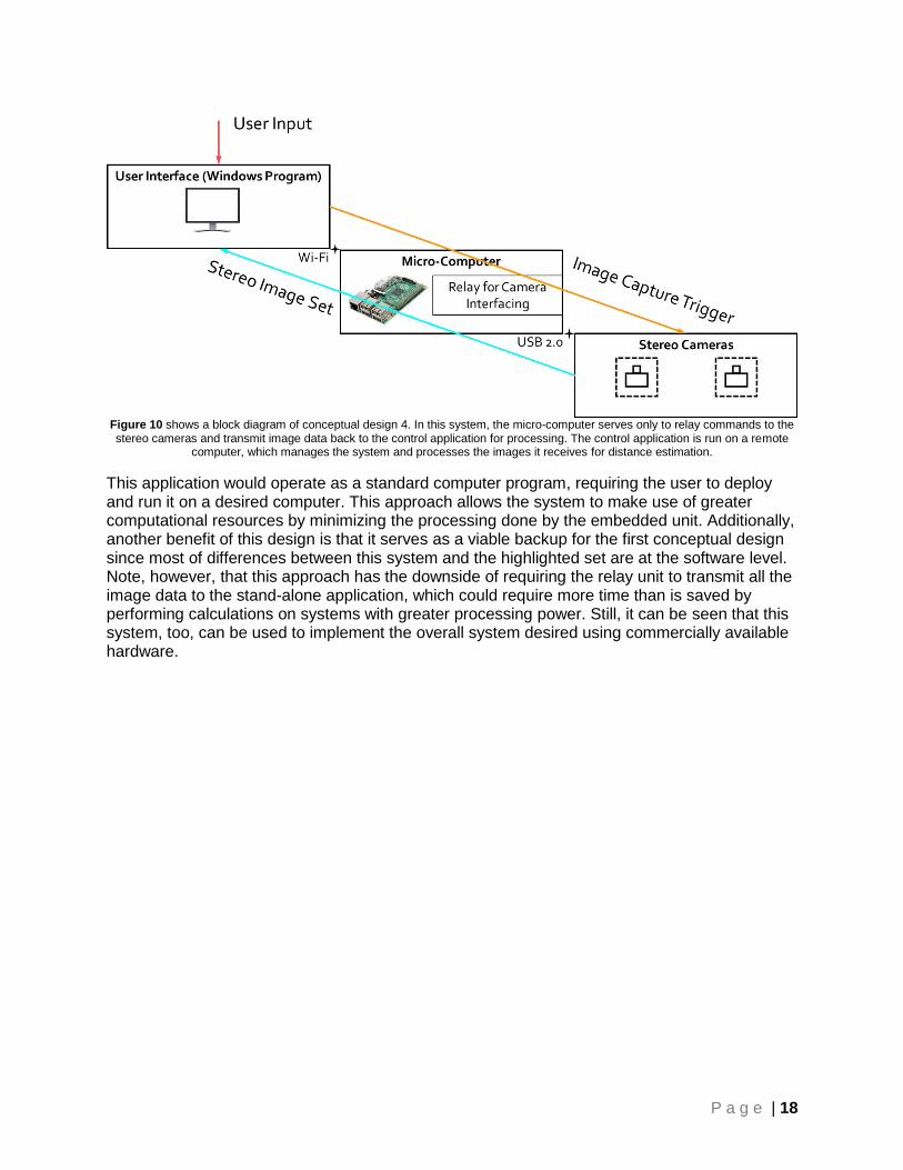
Design 4: Implementation of Image Processing Application Option 3 Another variation on the conceptual design outlined in Figure 7 is introduced with the third option examined for potential image processing platforms. In this design, though, the embedded controller merely serves to relay image data from the stereo cameras to a stand-alone computer application as shown in Figure 10.

P a g e | 18

Figure 10 shows a block diagram of conceptual design 4. In this system, the micro-computer serves only to relay commands to the stereo cameras and transmit image data back to the control application for processing. The control application is run on a remote

computer, which manages the system and processes the images it receives for distance estimation.

This application would operate as a standard computer program, requiring the user to deploy and run it on a desired computer. This approach allows the system to make use of greater computational resources by minimizing the processing done by the embedded unit. Additionally, another benefit of this design is that it serves as a viable backup for the first conceptual design since most of differences between this system and the highlighted set are at the software level. Note, however, that this approach has the downside of requiring the relay unit to transmit all the image data to the stand-alone application, which could require more time than is saved by performing calculations on systems with greater processing power. Still, it can be seen that this system, too, can be used to implement the overall system desired using commercially available hardware.

P a g e | 19

Section III: Summary of the Evaluation of the Conceptual Designs

Camera Type Selection For any of the systems outlined in the preceding section, the type of camera utilized (Webcam, Point-&-Shoot, etc.) intrinsically defines the quality of the stereo images processed by the system, how much data comprises each of the image sets retrieved, and other characteristics that merit approaching the choice of camera type as a distinct design decision. This is best accomplished by delineating which specific system characteristics are affected by camera hardware and determining their importance relative to each other within the scope of the given design. With this accomplished, a scaling system needs to be created for each attribute listed in order to numerically relate the camera types with respect to their different characteristics and specifications. For instance, based on the comparison of camera types found in the previous section, the following set of attributes for each type is created along with an associated rating scale: Image Resolution Because this is intended for 2-D positioning, only the horizontal image resolution of cameras is of interest, however the full resolution (horizontal resolution x vertical resolution) of cameras for photography is usually expressed in megapixels (MP). Therefore, the following scale is used to classify each camera type by its attainable image resolution.

1. Under 4 MP

2. 4-8 MP

3. 8-12 MP

4. More than 12 MP

Angular Field of View As with image resolution, only the horizontal range visible to a camera is of interest for the given application. Marketed values for this attribute typically indicate the diagonal field of view for the given unit, which is categorized into ranges by the following scale.

1. Under 70 degrees

2. 70-80 degrees

3. 80-90 degrees

4. More than 90 degrees

Lens quality Higher quality lenses are produced under tighter manufacturing constraints to minimize the effects of lens distortion on captured images. An improvement in this attribute is typically tied to increased unit costs. Average Unit Cost

1. Over $150

2. $125 - $150

3. $100 – 125

4. Under $100

Support for software control This attribute involves some risk for all camera types other than webcams, as only certain digital cameras provide the required functionality. On Linux operating systems, the gPhoto2 application can be used to remotely control some cameras using PTP, but the options available for control vary from camera to camera. The same is true when considering proprietary interfaces as well.

P a g e | 20

This owes to the fact that such units are typically operated manually, making remote operation a more advanced feature that is less frequently utilized by consumers. For each of the camera types considered for this application, the following rating scale is used to denote, in general, what portion of commonly marketed cameras of that type have documented support for PC control.

1. All units USB file transfer support only. 2. Few units support remote control. 3. A large portion of units support remote control 4. All units support remote control.

For instance: web cameras, which are intended for this purpose, are placed in the fourth category listed, while point-and-shoot cameras fall into the second because only a small portion of consumer models for this type are intended for remote operation.

Size The physical space occupied by the camera is of less concern relative to its imaging capability, but when mounting in stereo, the camera’s footprint is something that needs to be considered.

1. Over 75 in2

2. 50 – 75 in2

3. 25 - 50 in2

4. Under 25 in2 To determine the importance of these attributes relative to one another, the binary decision matrix in Table 1 is implemented.

Table 1: Binary decision matrix for relevant camera attributes. A cell value of 9 indicates that the attribute in the corresponding row is of greater importance than that of the corresponding column. A value of 1 indicates that the attribute in the corresponding column is of greater importance than that of the corresponding row, while a value of 5 indicates equal importance for the associated factors.

Cost Resolution Field of View

Lens Distortion

Software Control Size Total

Scaled (%)

Cost x 9 9 9 9 9 45 32

Resolution 1 x 9 9 5 9 33 20

Field of View 1 1 x 5 1 9 17 12

Lens Distortion 1 1 5 x 1 9 17 12

Software Control 1 5 9 9 x 9 33 20

Size 1 1 1 1 1 x 5 4

The binary decision matrix gives a rough idea of the relative importance of each camera attribute defined. The value of each cell on this table is determined based on a comparison of the design factors in the corresponding row and column. Each row is summed to produce its value in the “Total” column, which is then scaled to produce a column containing equally proportioned values that sum to 100%. For instance, the cumulative total of row summation values in the “Total” column of Table 1 is 150. To make the sum of the “Scaled (%)” column of the table to be 100, each value of the “Total” column is multiplied by a factor of 2/3 and adjusted so that the result is an integer value. When applying these scaled weight values in conjunction with the ranking system defined for each attribute considered, the camera type decision matrix in Table 2 is produced.

P a g e | 21

Table 2: Decision matrix for camera type selection based on attribute rankings and the relative importance weights from Table 1.

Camera Type

DSLR Point and Shoot Webcam

Attribute Relative

Weight (%) Rating Weighted

Rating Rating Weighted


Rating

Cost 32 2 64 4 128 4 128

Resolution 20 2 40 3 60 1 20

Field of View 12 4 48 2 24 2 24

Lens Distortion 12 3 36 2 24 1 12

Software Control 20 3 60 2 40 4 80

Size 4 2 8 4 16 4 16

Total 256 292 280

Elaborating more on Table 2, note that point-and-shoot and web cameras are closely ranked because they complement each other in terms of resolution and support for software control, both of which are weighted as equally desirable in the overall system. That said, point-and-shoot cameras have superior lenses and are intended for high resolution still photo capture, making them a better choice for this application. Also note that though the same argument can be made for DSLR cameras over point-and-shoot models, the increased price of these units is not set because they have a higher resolution, but rather because they offer additional features that will likely go unused in this application anyway. Basically, a single DSLR does not effectively double the imaging capability of 2 point-and-shoots, making this type of camera less desirable in terms of expense vs. functionality. Also note that rankings for prefabricated stereo cameras are omitted from Table 2. This is done intentionally as high resolution stereo units have prices that exceed the budget of this design, while most low-quality units are intended for producing “3D” images such as anaglyphs and do not allow for remote operation. Additionally, it was noted previously that such units have an immutable baseline distance between stereo lenses. Because these units are intended for ”3D” imaging, this baseline distance is small, not exceeding 10 cm, making them less applicable to the current application.

System Configuration Selection The organizational process enacted to help decide upon the camera type suited for this application is also applied to aid in the evaluation of the conceptual designs discussed in Section II. When considering the attributes and features important to the desired stereo imaging system, the following set of items is generated along with some associated rating scales: Remote Operation Will some means of external control be supported?

0. No

1. Yes

Versatility of Control Is the control interface for the system cross-platform?

0. The system interface is only accessible from a single computational system. 1. System interface allows for access from multiple types of devices.

P a g e | 22

Operational (User) Complexity What are the responsibilities of the end user?

1. Operating the system is a multi-step process that directs the user to trigger each camera to capture an image, move the files to a designated directory, and execute a processing application that displays calculation results.

2. After powering the system, the user is required to initiate a small number of processes that automatically (connect to and) interact with one another.

3. The system is essentially “Plug and Play”. Setting up and operating the system consists of providing power to it and following some general prompts and instructions.

Software Development Complexity How many software components make up the interface for this system?

1. System has several software components that must communicate across systems each other and exchange data.

2. System management application is written for 1 platform and broadcasts data to a pre-existing application

3. System management application is written and executed on 1 platform. Hardware Complexity Does the system require components other than those connected to its controller or those used to fix stereo cameras in place?

0. Yes

1. No

Team Preference Ranking ordered by the interest of group members in implementing each conceptual design. A binary decision matrix is again utilized to help determine the relative importance of these design considerations. The results of this process are shown in Table 3.

Table 3: Binary decision matrix for relevant conceptual design considerations. A cell value of 9 indicates that the attribute in the corresponding row is of greater importance than that of the corresponding column. A value of 1 indicates that the attribute in the

corresponding column is of greater importance than that of the corresponding row, while a value of 5 indicates equal importance for the associated factors.

Remote

Operation Operational Complexity

Software Complexity

Hardware Complexity

Versatility of Control

Team Pref. Total

Scaled (%)

Remote Operation

x 1 9 5 5 5 25 18

Operational Complexity

9 x 9 9 9 9 45 30

Software Complexity

1 1 x 9 1 5 17 10

Hardware Complexity

5 1 1 x 5 5 17 10


5 1 9 5 x 9 29 22

Team Preference

5 1 5 5 1 x 17 10

The scaled weights that result from the above table are combined with the ranking systems defined for each consideration to produce the design decision matrix in Table 4.

P a g e | 23

Table 4: Decision matrix for choice of conceptual design based on attribute rankings and the relative importance weights from Table

3.

Conceptual Design

1: Simple

Configuration 2: Virtual Stereo

(with slider) 3: Virtual Stereo

(with mirrors) 4: Image Relay

Apparatus

Attribute Relative

Weight (%) Rating Weighted




Rating

Remote Operation

18 1 18 0 0 1 18 1 18

Operational Complexity

30 2 60 3 90 2 60 2 60

Software Complexity

10 2 20 3 30 2 20 2 20

Hardware Complexity

10 1 10 0 0 0 0 1 10


22 1 22 0 0 1 22 0 0

Team Preference

10 4 40 3 30 1 10 2 20

Total 170 150 130 128

It should be noted that the lists of relevant attributes and considerations used to produce Tables 2 & 4 are analyzed because they are useful when comparing the relative strengths and weaknesses of the design options presented. They are not intended to serve as comprehensive collections spanning every positive or negative aspect of each alternative presented. Nevertheless, the process used to generate these decision matrices greatly helps to organize the decision making process for the design of the desired system. It brings into focus to key considerations, the relative importance of these elements, and how they manifest in each examined alternative. From this process, it is determined that the conceptual design diagrammed in Figure 7 of Section II, implemented with a pair of identical point-and-shoot cameras, should undergo further development in preparation for realization of the desired stereo imaging system.

P a g e | 24

Section IV: A Detailed Design of the Selected Conceptual Design

Theoretical Considerations The standard geometric model for a stereo vision system with parallel image planes is given in Figure 2. As noted with Equation 2, recovering the distance of a target based on its pixel disparity (d) in stereo images requires its physical focal length (f expressed in mm) of both cameras to be evaluated as a number of pixels (fpx). An estimation of fpx for a given camera can be obtained using the following equation, where ws represents the measured width of its image sensor

(3)

Note that this definition of fpx also serves to validate the equivalency of Equations 1 & 2 as geometrically

(4)

In either case, pixel disparity values (d) used to estimate distances to target objects using Equations 1 & 2 are determined by processing the stereo images from the cameras. Camera images are inherently subject to certain distortions caused by lens distortions, quantization noise, and other factors that introduce error when determining target disparities. From these, the relative distance error (Er in %) introduced by a single pixel error in the determination of d can be expressed as

(5)

Equation 5 implies that increasing the baseline distance between stereo cameras reduces the effect of disparity determination errors when recovering Z. However, because the two cameras have finite fields of view, an increase in distance separating them also increases the minimum distance that can be viewed by both cameras, expressed mathematically by Equation 6.

(6)

Thus, any set of cameras selected for this application must be separated by a baseline distance that leads to a low value of Er and an operable value for Dmin.

Hardware Clearly, the hardware component of greatest consequence in the system is the stereo camera set. For this application, the camera model found to have the best balance of the specifications indicated is the Canon PowerShot S80, shown in Figure 11.

P a g e | 25

Figure 11 shows the front view of a Canon PowerShot S80 8MP camera. Image from Amazon.com.

This camera has a nominal resolution of 3264 x 2448 (8 megapixels), resulting in an aspect ratio of 4:3. It also has variable zoom with minimum focal length of 5.8 mm and a 1/1.8” (8.89 mm diagonal) image sensor that helps to provide a wide diagonal angular field of view (75.2 degrees) compared to typical point-and-shoot models of the same resolution. This camera is also older with respect to the consumer market, meaning the purchase of two units still lies within the $300 design budget. The PowerShot S80 is supported by the gPhoto2 PTP backend that is available on Linux operating systems as mentioned in Section II. The Picture Transfer Protocol (ISO 15740) is a communication standard that allows digital cameras to transfer files to connected computers and other hosts without the need for model-specific device drivers. This protocol can also be used by the host system to control connected cameras, allowing the host to utilize them as a tethered periphery for image capture. Within Linux operating systems, gPhoto2 is a command line application that implements the PTP standard to this end. Most of the cameras supported by this application only allow for it to be used in management of image files already present within the camera’s internal storage. A subset of supported models, however, additionally allow for the tethered computer to trigger the capture of an image, change the digital zoom on the camera, and manipulate other settings available during the process of image collection. According to official gPhoto2 documentation, the Canon PowerShot S80 falls within this subset, making its inclusion in the overall system a substantial benefit. Using the camera specifications given above, it can be determined that at minimum zoom, the focal length of this unit in pixels is 2663 pixels and that its horizontal field of view is approximately θ = 63 lateral degrees. Based on these parameters, the minimum distance that can be viewed is approximately 80% of the baseline camera separation. Because this camera specifies a normal focus range of no less than 50 cm, a baseline distance of at least 62 cm is preferable. For convenience, a baseline separation of 1 m is selected. This value reduces the distance error estimated in Equation 6 to 0.185 % per pixel for distances of 5 m, but creates a dead zone for targets located less than 81 cm out from the apparatus. This is acceptable, however, as even though each camera is capable of imaging an object at this distance, such a target would most of the field viewed by each camera, and obscure objects positioned further

P a g e | 26

behind. The same logic can be applied for greater baseline separations as well, but implementing such distances requires a longer, more unwieldly mounting fixture to support the stereo cameras. Additionally, a nominal separation of 1 m simplifies Equations 1 & 2, making analysis of distance estimates within the system simpler by extension. The next piece of the hardware to be considered is the mechanism for mounting the stereo cameras. An apparatus is needed that securely holds the cameras in place at a specified distance apart. The stand design, modeled in Figure 12 below, aims to meet this need.

Figure 12: An overall view of the stereoscopic imaging apparatus. The stand shown supports a wooden board upon which are

mounted the stereo cameras and the Raspberry Pi image processing unit.

P a g e | 27

The stand consists of tripod that supports a wooden board with the stereo cameras mounted on either end. The shaft of the tripod will slide through a hole drilled through the board, a connection which will be supported by blocks bolted to the stand as laid out in Figure 13

Figure 13: A detailed view of the front of the stereoscopic imaging stand. The center hole of the board is sized such that it

encompasses the main shaft of the supporting tripod shown. Two holes are bored towards each end of the board, through which the clamp bolts for camera mounting are threaded. The numbers in this figure refer to corresponding items on the bill of materials, which

can be found in Section V.

The cameras are attached to the board by a clamp with an integrated bolt that screws into the tripod thread located on the bottom of the camera. The clamping bolt is the same type used for locking the position and alignment of bike seats, and by drawing the camera and mounting board together as shown, this component should provide the same functionality in this application. One concerning issue with this design is that the battery port for the camera is on the bottom of the camera, which is clamped to the top plane of the mounting board as discussed. The only way to access this port is to remove the camera from the board, which would require the system to be realigned and recalibrated each time one of the camera batteries dies. Fortunately, Canon manufactures a charging device for the chosen camera model, which will allow for the charging of camera batteries without unmounting them.

Image Processing Images from most digital cameras are JPEG formatted by default. Programmatically, this format translates to a two-dimensional array of RGB vectors: sets containing three values that indicate the respective amounts of red, green, and blue light that additively combine to form a color. In this color model, the primary colors red, green, and blue form an orthogonal basis set spanning a three-dimensional, cubic color space as modeled in Figure 14.

P a g e | 28

Figure 14 shows a geometric representation of the standard RGB color model. This color space is spanned by the primary colors

red, green, and blue, with black lying on the origin (0, 0, 0) and white positioned diagonally opposite as shown.

For example, if the 24-bit RGB vector in row zero, column zero of an image array has ordered values of {255, 0, 0}, then the top, left pixel in that image is red in color. When used to computationally process an image using the given format, color detection is implemented by identifying the Euclidean distance between a color of interest and the color of each pixel in the image. By masking out the distances that fall above a certain threshold as shown in Figure 15, regions of a specific color may be isolated within an image.

Figure 15: Simple demonstration of using color detection to isolate a region of interest within an image. The right image in this set is a binary mask of the red target contained in the left image. This binary mask can quickly be processed to determine the position of

the represented region within the original image.

Note by defining a color of interest corresponding to one of the vertices on the primary axes of the cube shown in Figure 14, two of the three RGB components for the target color are zero, which geometrically simplifies this method of color detection. Based on this observation, the stereo imaging apparatus will be configured to identify red targets, as blue and green are more prevalent colors within the indoor environments in which this apparatus will be tested. Also note that the use of this method merely highlights a region of interest (the target in our application) within a given image. To find the actual coordinates of the masked object within the image, blob detection algorithms that estimate the center of such regions will be used. These algorithms are implemented in the OpenCV image processing libraries available for C++ and python programming languages. OpenCV documentation suggests that the systems utilizing them meet at least the following minimum system requirements.

P a g e | 29

256 MB of RAM

50 MB of free hard disk space (for the package itself)

Processor speed of 900 MHz. From previous analysis of common micro-computers in Section II, it is seen any of the alternatives examined are capable of enacting the image processing required for the stereo vision system. Therefore, because of its low cost, and its abundant community documentation, a Raspberry Pi unit is selected to fill the role of the controller managing this system.

The User Interface The need for a user interface that manages the operation of this system has been discussed several times through the course of its design. With this in mind, LabView software was used to lay out a sample UI configuration to illustrate how such a program could guide the user through operating the system and implement the functions outlined. These are modeled in Figures 15 and 16 below.

Figure 16: Main Screen - Main interaction screen for the user.

Figure 16 shows the main screen of a potential graphic user interface for the system. The “Settings” button will be used to load and validate the connection strings used by gPhoto2 to access and control each camera. These connection strings are determined using the gPhoto2 command line interface, and are used by the software to identify and interact with associated cameras. The main screen has two image displays that are used to show the last image set captured by the stereo cameras. When the user wishes to collect a new image set from the cameras, they press the “Capture” button, which triggers the program to retrieve the requested images using the gPhoto2 PTP backend and update the image displays accordingly. The program will automatically search the image and overlay a marker on any target it finds. The user will be able to edit the placement of such markers, allowing them to manually correct for

P a g e | 30

errors in target identification. At this point, a press of the “Process” button triggers the program to apply Equation 1 to each target identified in the previous step, estimating their positions relative to the apparatus and plotting them on the “Graph” screen modeled in Figure 17.

Figure 17: Graph Screen - Displays multiple distance measurements on a plot.

This screen thus provides an overhead view of target positions as measured by the system. The plot will retain previous entries, which necessitates the “Clear Targets” control shown to refresh the display space. This control interface will be implemented as a web service hosted by the Raspberry Pi. To provide access to this service, the RPi will broadcast an ad-hoc SSID via a connected 802.11b/g/n wireless transceiver. The user of this application will be required to connect to it using a wireless device, but this process can be scripted for desktop environments and has the advantage of allowing the application to be accessed using standard web browsers. Touching on the design of this interface: JQuery UI is a freely available set of Javascript libraries that define a set of control objects including data plots and other features for more advanced web applications. Additionally, the web service must be able to access the gPhoto2 application for camera control within the Raspbian OS, and so PHP or other CGI scripting will need to be used within the application as well.

Stereo Camera Calibration The images produced by the stereo cameras in this system will be subject to a certain amount of distortion caused by imperfections in the lens of each unit. Such distortions usually cause

P a g e | 31

straight lines imaged by a given camera to appear curved when sampled by its image sensor. They are also mostly radial in nature, meaning that the amount a pixel is apparently shifted due to a given camera lens increases with respect to its polar distance from the lens’s/image’s center. The California Institute of Technology has developed a MATLAB toolbox capable of mapping these position shifts individual cameras using multiple pictures of a chess board (or other grid) taken from said camera. The algorithms in the toolbox prompt the user to identify points on the grid, and uses this data to extrapolate coefficients for radial and tangential distortion models that can be used to re-project undistorted images. These coefficients can be exported as a parameter set, which will be loaded into the UI program using the “Calibration” control mentioned previously to correct for single camera image distortions. Along with lens distortions, any misalignment between the stereo cameras will also produce inaccuracies in calculations based on the stereo image sets collected from it. The MATLAB toolbox used to identify lens distortions for individual cameras can also be used to determine such offsets so that they can be corrected for using image processing, but implementing such corrective measures adds execution time to the processing of images. To this end, it is more prudent to mitigate the effect of misalignments by physically altering the orientation of cameras as they are mounted. For instance, when an object is located a great enough distance from a camera that the light rays from the object to the camera lens are parallel, the object is said to be located at infinity distance. For a stereo camera configuration, objects located at infinity distance exhibit no disparity between images from the cameras. Thus, when attempting to ensure the proper alignment of the stereo cameras in the given design, objects that lie at infinity distances (those at least 3.5 to 4 orders of magnitude greater than the 5.8 mm minimum camera focal lengths) will be photographed. Any disparity in the images of such objects corrected for by altering the surface of the mounting board (element 5 Figure 13), using shims, and adjusting the rotation of each camera on its mounting bolt (element 3 of Figure 13) using temporary set screws. Then, having secured the alignment of the stereo cameras by applying clamping force to their mounting bots, an offset compensation scheme with reduced computational complexity can be applied to further mitigate remaining errors. To elaborate on what “an offset compensation scheme with reduced computational complexity” entails, consider the image shown in Figure 18. In the given figure, targets are placed at known distances from the camera apparatus, and the disparity observed for each target viewed is recorded. Then, by interpreting B, xo and θ as constants intrinsic to system hardware and redefining Equations 1 & 2 as follows,

(7)

the value of K can be linearly interpolated from experimental values of variables D and d. Clearly, this method of system calibration is more mechanically complex, but using Equation 7 with a calibrated value for K accounts for stereo camera alignment errors without resorting to more complex software methods of offset correction.

P a g e | 32

Figure 18: Example calibration image taken by one camera of a stereo set. In this image, the red targets shown are positioned at

known distances.

P a g e | 33

Section V: Design Implementation

Construction of the Apparatus The system was initially constructed according to the design shown in Figure 12, but was modified in response to issues encountered during calibration and testing. Most of the modifications to the original design relate to the mounting of the stereo cameras, as noted in Figure 20.

Figure 19 highlights the camera mounting featrues altered with respect the original system design in Figure 12.

The first major change in how the cameras are mounted is that instead of being secured directly to the mounting board, the cameras are seated on adjustable platforms. The distance between each platform corner and the underlying mounting surface may be altered by changing the separation of the two nuts supporting that corner. This design alteration allows for much more precise changes to the roll and pitch of each camera to be made when aligning them. Also note from Figure 19 that the clamping bolts allocated to secure the cameras to their mounting surface in the original design were replaced with standard ¼”-20 carriage bolts to reduce hardware costs. It was found during construction that tightening a nut and lock-washer set against the bottom of the mounting surface as shown exerts sufficient clamping force to prevent the cameras from rotating on their associated mounting bolt. Lastly, observe that the two inch thick mounting board in the original design is replaced by a ¼” steel plate. This alteration was made because the force exerted by the nuts used to change the height of the mounting platforms was sufficient to warp the board along its length. A 1/8” steel plate was deemed to be susceptible to the same deformations, so the given plate was fabricated and installed. This represented an unintended setback for the project overall as it required the cameras to be re-aligned on the new mounting surface. Even with the substitution of a steel mounting plate, the full weight of the apparatus is only 30 pounds. This is below the 50 pound weight limit originally given as a general requirement for the apparatus. The final realization of the given design is shown below in Figure 20.

P a g e | 34

Figure 20: Final iteration of the design shown in Figure 12 for a stereo vision ranging apparatus.

Aside from the changes discussed previously, this apparatus shown is a serviceable realization of the design viewed in Figure 12. The two cameras are connected to a Raspberry Pi B2, which relays initialization, capture, and image retrieval commands to them in response as users interact with the web service it hosts. This web service is accessed by connecting a client to the local network managed by the Belkin router on which the Pi sits, a process detailed further in Accessing the User Interface (page 41). Lastly, it was noted when originally considering how to mount the stereo cameras that the ability to power these units without removing their batteries for charging was of critical importance. To this end, power packs were obtained that replace the 7 VDC batteries of each camera with a module that converts 120 VAC power (from a standard wall outlet) to this operational output. The installation of these modules allows the stereo cameras to remain mounted permanently, maintaining their calibrated alignment by ensuring a constant power supply.

Stereo Camera Alignment Once affixed, the stereo cameras were aligned such that their optical axes are parallel in three-dimensional space. Again, this involves aligning the cameras such that objects located sufficient distances from the apparatus exhibit no disparity in image sets. For the given camera units and baseline separation, it can be determined from Equations 1 & 2 that with each camera at minimal zoom (f = 5.8 mm), the minimum distance at which objects should exhibit less than one pixel of disparity is just over 2.7 km. To test this condition as alterations to camera alignment were made, images of the Indiana-Michigan Power building in downtown Fort Wayne were taken from IPFW campus. Using Google Earth, the linear distance between these two points was estimated to be over 5 km, validating the indicated landmark as a suitable alignment target. After each adjustment to the alignment of a camera, this building was imaged by both cameras and the results overlaid using Paint.net software as shown in Figure 21.

P a g e | 35

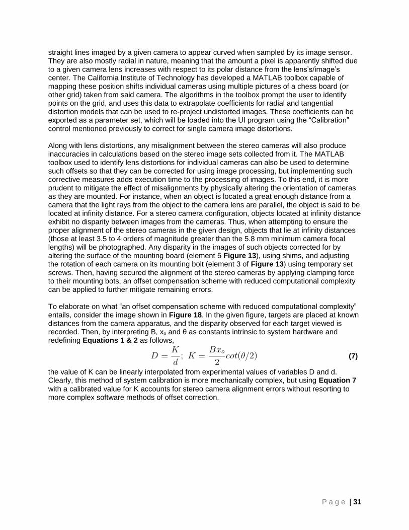
Figure 21: Portion of an image produced by overlaying the individual images from a stereo set. The skyscrapers shown are located

sufficiently far from the stereo baseline to exhibit no disparity, indicating that the optical axes of the cameras are parallel to each other.

With the cameras properly aligned, the given structure appears at the same coordinates in both images, while closer objects exhibit a lateral disparity as desired. Having ensured their alignment, the Powershot units were secured in place by significantly tightening their mounting bolts and applying hot glue to their bases to inhibit further motion.

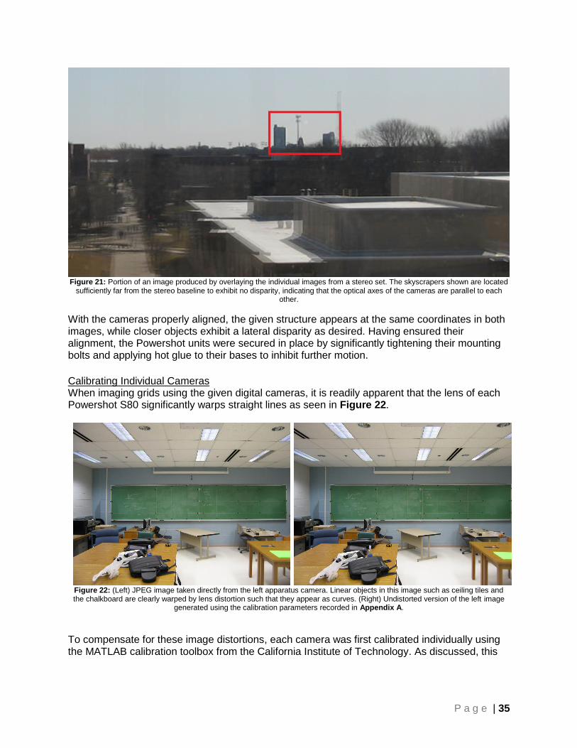
Calibrating Individual Cameras When imaging grids using the given digital cameras, it is readily apparent that the lens of each Powershot S80 significantly warps straight lines as seen in Figure 22.

Figure 22: (Left) JPEG image taken directly from the left apparatus camera. Linear objects in this image such as ceiling tiles and the chalkboard are clearly warped by lens distortion such that they appear as curves. (Right) Undistorted version of the left image

generated using the calibration parameters recorded in Appendix A.

To compensate for these image distortions, each camera was first calibrated individually using the MATLAB calibration toolbox from the California Institute of Technology. As discussed, this

P a g e | 36

toolbox uses multiple images of a chess board taken by a specific camera, such as those shown in Figure 23, to map pixel displacements caused by the lens of that unit.

Figure 23: Mosaic of chess board images used to calibrate the left camera in the given system. These images were processed by

the referenced camera calibration toolbox to extrapolate a model of distortions associated with the lens of the given camera.

Manually identifying the grid corners in each of the above images allows this tool to extrapolate coefficients for the distortion model described previously. Enacting this calibration procedure for both cameras output the intrinsic camera parameters recorded in Appendix A. From these, the program was able to generate the following graphical representations depicting how lens distortions warp images as they are taken using the given cameras.

P a g e | 37

Figure 24: Plots of the distortion model for each of the system’s stereo cameras. Black circles represent a displacement contour,

meaning pixels at specific x and y image coordinates are displaced by the magnitude of the contour on which they lie in the direction of the blue arrows shown. The star on these plots represents the center coordinates (1632, 1224) of camera images, while the circle

shows the principle point of scenes projected through the camera’s lens.

From Figure 24, it is clear that towards the center of each camera lens, there is little distortion, while pixel displacements become larger as their polar distance from the principle point increases. The given plots reveal that the observed lens distortions have a relatively large impact towards the edges of camera images, laterally displacing points by up to 50 pixels. Left uncorrected, this would represent a significant source of error when using this system for range estimation, requiring compensation to be applied as stereo images are processed. To this end, the intrinsic camera parameters identified by the calibration procedure for each unit were exported and used within the user interface to more accurately interpret the positions of targets identified within image sets. For more details regarding how the parameters were used in this context, refer to the Results Plot portion of the following analysis of the user interface for this system.

Calibrating the Overall System To calibrate the overall system, an experimental method based on images of multiple point sources was utilized similar to that used by Mahammed, Melhum, and Kochery. Point sources are objects such as LEDs or the corners of grid patterns that appear as single pixels or small, easily differentiable regions on images. Most of the calibration data for this apparatus was collected from images of a 20”x16” grid created by stretching thin strings horizontally and vertically over a chalkboard as shown in Figure 25.

P a g e | 38

Figure 25: One of the image sets used to calibrate the stereo cameras. Calibration images focus on intersection points on the

imaged grid, which lie at known locations relative to the apparatus itself. These images are undistorted versions of those originally taken by the stereo cameras. They were re-projected to compensate for the lens distortions of each camera diagramed in Figure

24.

As described with the above figure, images of calibration grids were undistorted using MATLAB to compensate for line warping caused by the lens of each camera. As a result of this process, the strings in the given image set appear as linear bands of 3-5 white pixels against a backdrop of green. This allows intersection points on the grid they form to be more easily determined when zooming in on the individual images. Once identified, the image coordinates of each intersection point was compared to its physical coordinates (relative to pivot axis of the apparatus) to experimentally correlate observed disparity (d) values with their known ranges (Z). Performing this experiment for a sequence of known ranges produced the data recorded in Appendix B; which, in turn, was used to generate log-log plot in Figure 26.

Figure 26: Log-Log plot of disparities observed for calibration grid points relative to their distance from the pivot axis of the

apparatus tripod, perpendicular to the camera baseline. The data used to generate this plot and that shown in Figure 27 can be viewed in Appendix B

Logd = -1.00127*LogZ + 3.96049

2.4

2.5

2.6

2.7

2.8

2.9

3

3.1

3.2

3.3

3.4

0.6 0.7 0.8 0.9 1 1.1 1.2 1.3 1.4 1.5 1.6

Log(

d)

Log(Z)

Recovering Z

P a g e | 39

From the linear regression in Figure 26, it can be determined that the calibrated relationship between Z (expressed in feet) and d from Equations 1 & 2 is the exponential function

(8)

This relationship is very close to that approximated using Equation 3, and implies that at the system baseline distance of 3.333 feet (1.016 m), the calibrated value of fpx in Equation 2 would be approximately 2708, just 43 pixels above the predicted value of this quantity. It is also known that the undistorted image coordinates (xi, yi) are projections of points with coordinates relative to camera I (Xci, Yci, Zci) such that

(9)

Given that Equation 8 outputs an estimate of Zci for conjugate points in stereo images, the same image sets used to calibrate the system for range measurements can also be used to calibrate it for recovering the lateral (X) positions of targets. To enact this calibration, both x coordinates for each calibration point viewed commonly by both cameras were averaged and compared to the known ratio of that point’s physical X and Z coordinates (with X = 0 located on the pivot axis of the apparatus). The results of this analysis are depicted in Figure 27 below.

Figure 27: Plot of mean image coordinates for calibration grid points relative to the ration of their real-world X and Z coordinates.

The data used to generate this plot and that shown in Figure 26 can be viewed in Appendix B

As seen in Figure 27, a linear regression can be applied to the data sets plotted for each camera. The linear regression of calibration data from left camera images implies that

ẍ = (xl + xr) / 2;

X = Z*(ẍ - 1717)/2723 (10)

y = 2,723.051556x + 1,716.5065

0

500

1000

1500

2000

2500

3000

-0.5 -0.4 -0.3 -0.2 -0.1 0 0.1 0.2 0.3 0.4 0.5

ẍ=

(x_l

+ x

_r)/

2 (

px)

X/Z

Recovering X

P a g e | 40

where Z is the output of Equation 8 and xl + xr refers to the sum of the lateral image coordinates of a given target. After completing the calibration procedures outlined, Equations 10 & 11 were tested against the majority of the data points used to derive them. The results of this test are depicted below in Figure 28.

Figure 28: Plot of calibration grid points with X and Z coordinates estimated by Equations 10 & 8 respectively.

Observe that using the given equations to estimate the positions of the grid points originally used for calibration projects these locations onto planes that are slightly skewed with respect to the X axis. Because each calibration image consisted of a planar grid of point sources positioned parallel to the system’s baseline, each line of points in the above plot should be parallel to the X axis, not sloped as shown. To compensate for this, the average slope (m) of the linear regressions in Figure 28 was calculated and used to adjust Z values recovered using Equation 7 such that

m = 0.67958; Z = Zold + mX

(11)

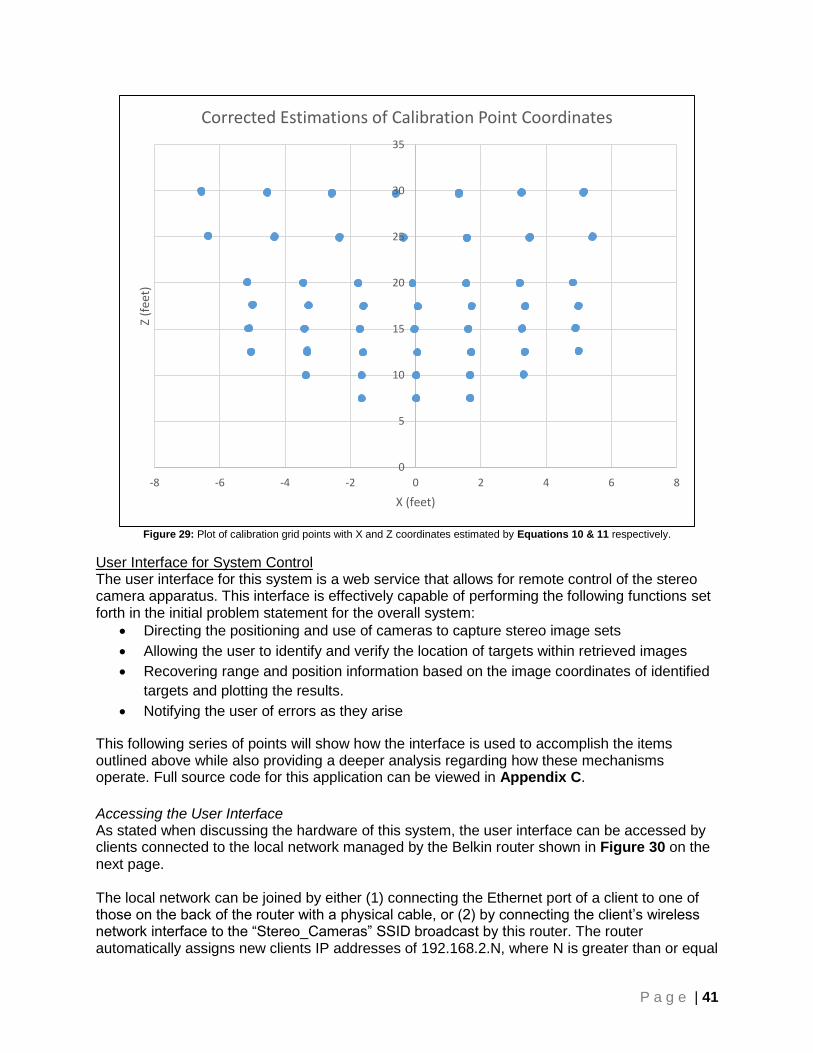
Applying this adjustment to the data points plotted in Figure 28 produces the corrected version displayed in Figure 29, in which the skew previously observed in the grid point location estimates is greatly reduced and nearly parallel to the X axis as desired.

y = -0.053243x + 7.486277

y = -0.056801x + 10.010389

y = -0.064134x + 12.526160

y = -0.065572x + 15.049549

y = -0.080693x + 17.521066

y = -0.072251x + 20.012409

y = -0.075811x + 24.976362

y = -0.075156x + 29.809821

0

5

10

15

20

25

30

35

-8 -6 -4 -2 0 2 4 6 8

Z (f

eet)

X (feet)

Preliminary Estimations of Calibration Point Coordinates

P a g e | 41

Figure 29: Plot of calibration grid points with X and Z coordinates estimated by Equations 10 & 11 respectively.

User Interface for System Control The user interface for this system is a web service that allows for remote control of the stereo camera apparatus. This interface is effectively capable of performing the following functions set forth in the initial problem statement for the overall system:

Directing the positioning and use of cameras to capture stereo image sets

Allowing the user to identify and verify the location of targets within retrieved images

Recovering range and position information based on the image coordinates of identified

targets and plotting the results.

Notifying the user of errors as they arise

This following series of points will show how the interface is used to accomplish the items outlined above while also providing a deeper analysis regarding how these mechanisms operate. Full source code for this application can be viewed in Appendix C.

Accessing the User Interface As stated when discussing the hardware of this system, the user interface can be accessed by clients connected to the local network managed by the Belkin router shown in Figure 30 on the next page. The local network can be joined by either (1) connecting the Ethernet port of a client to one of those on the back of the router with a physical cable, or (2) by connecting the client’s wireless network interface to the “Stereo_Cameras” SSID broadcast by this router. The router automatically assigns new clients IP addresses of 192.168.2.N, where N is greater than or equal

0

5

10

15

20

25

30

35

-8 -6 -4 -2 0 2 4 6 8

Z (f

eet)

X (feet)

Corrected Estimations of Calibration Point Coordinates

P a g e | 42

to 5, using a standard DHCP pool with a subnet mask of 255.255.255.192. The client can then access the system’s web interface by navigating to 192.168.2.2 using the web browser of their choice.

Figure 30: Block diagram displaying the interconnections between the different pieces of hardware in the system.

The user interface application is composed mostly of standard HTML, Javascript, and CSS code that is sent to clients by Lighttpd (pronounced as lighty) web server application. Lighttpd is a fast, lightweight web service for Linux operating systems that is strictly limited in terms of what system functions it has permission to access. By default, this service uses the directory /var/www as the root directory, sometimes referred to as the “document root” for incoming requests. When a client web browser requests the file http://192.168.2.2/index.html, the Pi responds with the contents of /var/www/index.html, which the browser interprets and renders accordingly. For this application Lighttpd was also configured to execute php scripts and shell (Linux command line) scripts on the server side of this exchange. These scripts allow the server

P a g e | 43

to dynamically generate some of the content it sends to the client, but allowing them to execute properly within Linux can require additional configuration procedures. For instance, due to the limited permissions associated with the web service in Linux, php and shell scripts must be contained in the /var/www directory and its subdirectories or the server will not be authorized to access them. Additionally, to allow the Lighttpd application to use gphoto2 and access the Canon units over USB connections, the service needed to be granted additional permissions to do so. The system can be altered to loosen these restrictions in general but it should be noted that these limitations are put in place intentionally to minimize the damage attackers can cause should they penetrate the web service.

System Home Figure 31 on the next page is a screenshot of the home page of the user interface as well as an interaction diagram depicting how it is used by client browsers to interact with the Raspberry Pi. The text shown at the top of the page provides users with the following general instructions regarding proper operation of the stereo camera apparatus:

1. When both cameras are first activated, their lenses may be retracted.

If this is the case, press the 'Initialize' button below to set up the cameras for image

collection.

2. Point the system cameras in the direction of the desired target object(s).

3. Retrieve a stereo image set from the cameras by pressing the "Capture" button.

4. From this page, click on one of the images displayed below to open a target

identification dialogue.

5. Once targets have been found, click the "Process" button to get the distance estimates.

Below this text are a small number of controls, each of which corresponds to an operation from the list above. The first of these controls is the “Initialize” button. As shown in Figure 31, pressing this button sends the Raspberry Pi a request to execute the CameraInit.sh shell script stored in the cgi-bin/ subdirectory of /var/www/. This script effectively queries the USB ports to which the cameras are connected to find the device ID number Linux assigned to them as they were detected by the system. These ID numbers are then used in a gphoto2 command that places the cameras in “capture” mode, extending their lenses in preparation for image collection.

P a g e | 44

Figure 31: Appearance of the System Home screen for the web interface implemented as well as an interaction diagram depicting

its relationship to the Raspberry Pi server. This screen provides an overview of how to use the system and several operational controls. These controls send HTTP GET requests (blue) to the server and receive responses (green) accordingly. Thicker arrows

on the interaction diagram indicate that the given request/response involves the client browser navigating to another UI screen.

P a g e | 45

Below the other control buttons shown is a table displaying previews of the last stereo image set collected by the system cameras. Note that these images are not corrected for lens distortion. The program, instead, determines the undistorted position of points marked by the user as it processes them to generate the results plot discussed later. The images themselves are stored in ImageSet/ subdirectory of /var/www, which is specially configured so that Lighttpd instructs client web browser not to cache images from this location. To elaborate, browsers normally store images and other page content on the client machine to reduce traffic to the server. This behavior is not desirable for stereo image sets, however, so the given directory is configured such that the user always receives the most recent version of files contained therein. Finally, below the stereo image preview are two text strings indicating the number of targets the user has identified within each image. These numbers are updated as System Home is loaded by calling the targetCounts.php script also located in the document root. This script executes and returns the indicated values to the page, which updates the text below each image accordingly.

Camera Trigger The control associated with item 3 of the main instruction list is the “Capture” button. This control navigates to /cgi-bin/CameraControl.html, depicted in Figure 32, which immediately calls the CameraTrigger.sh shell script as it loads.

Figure 32: Appearance of the Camera Trigger screen for the web interface implemented as well as an interaction diagram depicting

its relationship to the Raspberry Pi server. The meanings of the colors and line weights of interaction arrows are consistent with those described in Figure 31

P a g e | 46

The script triggers both cameras to capture images using gphoto2 and downloads them to the ImageSet/ directory discussed, then sends an error code to the client web browser. Note that the “Images Captured, Downloading…” message is not shown on the screen as this process commences. It takes the stereo cameras approximately 4.5 seconds on average for the cameras to record and image once triggered, and another 4.5 to concurrently download them. Because this represents a significant wait time for the user, the second label automatically appears after 5 seconds to provide some form of feedback. The given duration represents the longest interval spent processing by the interface application; and even though it exceeds the wait time originally set forth as a system specification, this cannot be helped as the camera hardware itself bottlenecks this procedure. Still, every other user interaction with this application takes less than 3 seconds to complete, so all processes not related to image capture fall within the time limit set. If the response sent by the image capture script indicates that it executed successfully (<ecode> = ‘0’), the page automatically redirects the browser back to system home; if not, the user is notified that an error occurred by a visual alert. Another indication of failure can be seen if the given page redirects to System Home, but no images load into the preview panes. If this occurs multiple times, it is often worthwhile to cycle power to the system and reinitialize the cameras before attempting another image capture.

User Targeting Item 4 from the main instruction list points out that clicking on either of the preview images seen in Figure 31 directs the client browser to the User Targeting screen shown in Figure 33.

P a g e | 47

Figure 33: Appearance of the User Targeting screen once it loads a camera image. This screen allows users to identify targets

directly on loaded images and saves their image coordinates for later processing.

On this page, the user can identify and edit targets directly on images from the stereo cameras. The page takes as input an HTTP GET argument of <position>, which it uses to load the proper camera image as it renders. When the rendered image is clicked, a small blue square indicating the selection point appears. Users indicate that the selected region represents a target by clicking the “Mark As Target” button shown in the figure. This action expands the cursor to a large, red rectangle that the user adjusts to envelop the target on the image using the controls shown in Figure 34.

P a g e | 48

Figure 34: After the user clicks the “Mark As Target” button, a rectangle is painted on the image that the user adjusts to envelop the selected item. The user does this by changing the Top, Bottom, Left, and Right coordinates of the rectangle via the controls shown.

These controls appear next to any region marked as a target in this way.

Because this dialogue employs rectangular identification markers, it should be noted that structured targets such as circles and rectangles are handled best by the system. Shaped targets with straight defined edges are simple to visually match with the edges of the rectangular markers drawn, allowing users to conveniently and accurately designate target points via the process outlined. After a target is identified in an image, the user is directed to save their edits and move to the other image and repeat this process. Each time the “Save Edits” button is pressed, the height and width of all rectangles marked on the image are saved along with the image coordinates of their upper left corner by calling the ExportCSV script referred to in Figure 35.

P a g e | 49

Figure 35: Interaction diagram for the User Targeting screen on the system interface. The meanings of line colors and weights on

this interaction arrows are consistent with those described in Figure 31. Additionally, pink and orange arrows represent HTTP POST requests and responses respectively.

The ExportCSV routine, shown by the lower pink request arrow, simply receives this input from the browser in an HTTP POST message and writes the input to a file stored on the Raspberry Pi. The figure also reveals that each time this page loads, it retrieves data for previously rectangles using the ImportCSV routine (the upper POST request) and draws them on the image. In this way, the user can mark multiple targets on an image while the application can track which rectangles correspond between the stereo images.

Results Plot Once the user has identified the position of each target visible in a stereo image set, they can click on the “Process” button located on the System Home page. This button directs the client browser to ResultsPlot/index.php under the document root. As this page loads, php code on the Raspberry Pi first calls a C++ program that individually reads the rectangle data files saved by the User Targeting dialogue for each image. The program then determines coordinates of each rectangle’s center point on the image and calculates their undistorted locations using the distortion parameters identified for each camera during calibration (Appendix A). Php code on the server then retrieves the output of this program and calculates the disparity (d) between corresponding (undistorted) center points. Finally, it estimates the X and Z coordinates for each associated target using Equations 10 & 11 and queues them to be drawn on the plot shown in Figure 36.

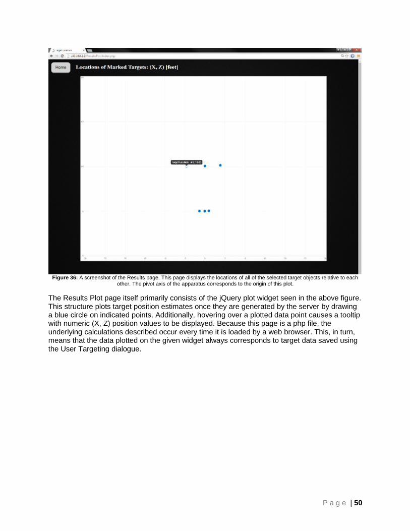
P a g e | 50

Figure 36: A screenshot of the Results page. This page displays the locations of all of the selected target objects relative to each

other. The pivot axis of the apparatus corresponds to the origin of this plot.

The Results Plot page itself primarily consists of the jQuery plot widget seen in the above figure. This structure plots target position estimates once they are generated by the server by drawing a blue circle on indicated points. Additionally, hovering over a plotted data point causes a tooltip with numeric (X, Z) position values to be displayed. Because this page is a php file, the underlying calculations described occur every time it is loaded by a web browser. This, in turn, means that the data plotted on the given widget always corresponds to target data saved using the User Targeting dialogue.

P a g e | 51

Section VI: Testing

Position Estimate Accuracy The first aspect of the system tested was the relative accuracy of its target coordinate estimations. This analysis was partially accomplished during apparatus calibration when using Equations 10 & 11 to estimate the positions of calibrated grid points. Again, these points were known positions, meaning the relative error (in %) associated with the estimated location of each point is defined as

(12)

The two datasets produced by calculating these errors for the calibration points recorded in Appendix B are plotted on the histograms in Figure 37.

Figure 37: Histogram of estimation errors for calibration point locations from the apparatus calibration data in Appendix B.

The red lines on the histograms above highlight that when estimating the X coordinates of calibrated point sources, 110 out of 120 estimates were accurate to within 1%. Similarly, when estimating the Z coordinates of known points, 142 out of 163 estimates were accurate to within 2%. The next element of the system tested was the accuracy to which a user can identify target positions within the User Targeting dialogue on the system’s web interface. To evaluate this, the stereo image sets arrayed in Figure 38 were collected and interpreted using this interface.

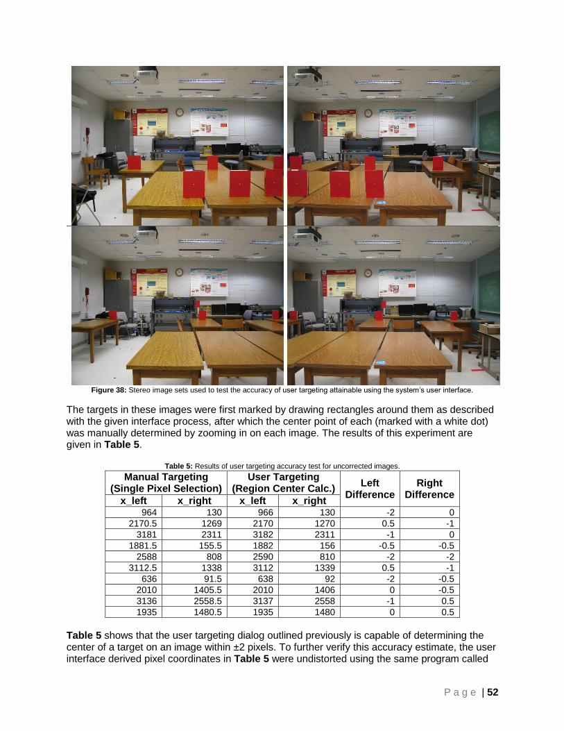
P a g e | 52

Figure 38: Stereo image sets used to test the accuracy of user targeting attainable using the system’s user interface.

The targets in these images were first marked by drawing rectangles around them as described with the given interface process, after which the center point of each (marked with a white dot) was manually determined by zooming in on each image. The results of this experiment are given in Table 5.

Table 5: Results of user targeting accuracy test for uncorrected images.

Manual Targeting (Single Pixel Selection)

User Targeting (Region Center Calc.)

Left Difference

Right Difference

x_left x_right x_left x_right 964 130 966 130 -2 0

2170.5 1269 2170 1270 0.5 -1

3181 2311 3182 2311 -1 0

1881.5 155.5 1882 156 -0.5 -0.5

2588 808 2590 810 -2 -2

3112.5 1338 3112 1339 0.5 -1

636 91.5 638 92 -2 -0.5

2010 1405.5 2010 1406 0 -0.5

3136 2558.5 3137 2558 -1 0.5

1935 1480.5 1935 1480 0 0.5

Table 5 shows that the user targeting dialog outlined previously is capable of determining the center of a target on an image within ±2 pixels. To further verify this accuracy estimate, the user interface derived pixel coordinates in Table 5 were undistorted using the same program called

P a g e | 53

by the application to correct points displaced by lens distortions. Then, the images in Figure 38 were re-projected, using the compensation parameters in Appendix A, so that target centers could again be manually identified. A similar comparison of these two data sets is given in Table 6, which reports that the ±2 pixel accuracy associated with targets marked on distorted images leads to a ±2.5 pixel accuracy on their corrected equivalents.

Table 6: Results of user targeting accuracy test for corrected images.

Manual Targeting (Single Pixel Selection)

User Targeting (Region Center Calc.)

Left Difference

Right Difference

x_left x_right x_left x_right 956.5 80 958.8534 80.27413 -2.35336 -0.27413

2173.5 1268.5 2173.025 1269.006 0.474919 -0.50572

3238.5 2319 3239.581 2318.92 -1.0812 0.079947

1883 105.5 1883.404 105.8298 -0.40403 -0.32976

2607.5 794 2609.586 796.5731 -2.0855 -2.57315

3167 1336 3166.082 1337.214 0.91773 -1.21399

615.5 39 617.2518 39.73356 -1.75178 -0.73356

2010 1405 2010.895 1405.843 -0.8955 -0.84314

3189 2575.5 3190.704 2575.526 -1.7044 -0.02572

1935 1480.5 1935.474 1479.966 -0.47426 0.53433

Lastly, the difference between the x_left and x_right columns in Table 6 were used to recover target locations according to Equations 10 & 11. The X and Z coordinates output from these equations were then compared to the known location of each target from Figure 38 to produce Table 7.

Table 7: Position estimates for targets shown in Figure 38 as well as associated estimation errors.

Known Position (feet) Estimated Position (feet) Estimation Errors (%)

X Z X Z EX EZ

-4.5 10 -4.55 10.05 0.43 0.52

0 10 0.02 10.07 0.12 0.71

3.875 10 3.86 10.15 0.12 1.51

-1.333 5 -1.36 5.03 0.19 0.67

0 5 -0.02 5.02 0.18 0.48

1 5 0.98 5.05 0.15 0.97

-7.75 15 -8.03 15.21 2.89 1.39

0 15 -0.04 15.04 0.32 0.23

6.5 15 6.34 15.22 1.49 1.48

0 20 -0.06 19.96 0.46 0.18

Table 7 denotes a peak error of 2.9% in estimates of target locations generated using the system’s user interface with the image sets from Figure 38. This is well below the 5% accuracy goal set forth in the initial specifications for this system, indicating that the given user targeting implementation performs as desired.

Repeatability Considerations Another system attribute worth examining is its repeatability with respect to how the cameras are initialized. It was given with Figure 31 that when the cameras are first supplied power, they must be placed into “capture” mode, which extends their lenses for image retrieval. The object of the following test is to determine if targets appear to shift within the same imaging field as power is cycled and the system re-initializes. The test focused on the five targets arrayed in Figure 39 , the positions of which were recorded in Table 8.

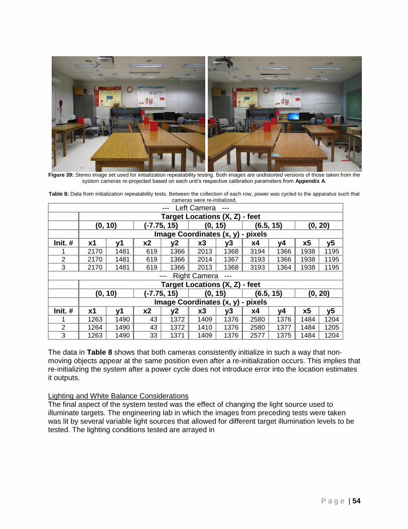
P a g e | 54

Figure 39: Stereo image set used for initialization repeatability testing. Both images are undistorted versions of those taken from the

system cameras re-projected based on each unit’s respective calibration parameters from Appendix A.

Table 8: Data from initialization repeatability tests. Between the collection of each row, power was cycled to the apparatus such that cameras were re-initialized.

--- Left Camera ---

Target Locations (X, Z) - feet

(0, 10) (-7.75, 15) (0, 15) (6.5, 15) (0, 20)

Image Coordinates (x, y) - pixels

Init. # x1 y1 x2 y2 x3 y3 x4 y4 x5 y5 1 2170 1481 619 1366 2013 1368 3194 1366 1938 1195

2 2170 1481 619 1366 2014 1367 3193 1366 1938 1195

3 2170 1481 619 1366 2013 1368 3193 1364 1938 1195

--- Right Camera ---


(0, 10) (-7.75, 15) (0, 15) (6.5, 15) (0, 20)


Init. # x1 y1 x2 y2 x3 y3 x4 y4 x5 y5 1 1263 1490 43 1372 1409 1376 2580 1376 1484 1204

2 1264 1490 43 1372 1410 1376 2580 1377 1484 1205

3 1263 1490 33 1371 1409 1376 2577 1375 1484 1204

The data in Table 8 shows that both cameras consistently initialize in such a way that non-moving objects appear at the same position even after a re-initialization occurs. This implies that re-initializing the system after a power cycle does not introduce error into the location estimates it outputs.

Lighting and White Balance Considerations The final aspect of the system tested was the effect of changing the light source used to illuminate targets. The engineering lab in which the images from preceding tests were taken was lit by several variable light sources that allowed for different target illumination levels to be tested. The lighting conditions tested are arrayed in

P a g e | 55

Table 9. Following

P a g e | 56

Table 9, the coordinates of the five targets visible in each associated image set are recorded in

P a g e | 57

Table 10.

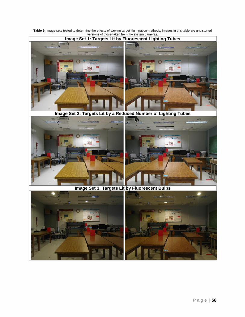
P a g e | 58

Table 9: Image sets tested to determine the effects of varying target illumination methods. Images in this table are undistorted versions of those taken from the system cameras.

Image Set 1: Targets Lit by Fluorescent Lighting Tubes

Image Set 2: Targets Lit by a Reduced Number of Lighting Tubes

Image Set 3: Targets Lit by Fluorescent Bulbs

P a g e | 59

Image Set 4: Targets Illuminated by Reflected Light

Image Set 5: Targets Lit by Camera Flash

P a g e | 60

Table 10: Pixel coordinates of targets shown in image sets from

P a g e | 61

Table 9

--- Left Camera ---


(0, 10) (-7.75, 15) (0, 15) (6.5, 15) (0, 20)


Set x1 y1 x2 y2 x3 y3 x4 y4 x5 y5 1 2170 1481 619 1366 2013 1368 3194 1366 1938 1195

2 2170 1481 619 1366 2014 1367 3194 1366 1939 1195

3 2170 1481 619 1366 2014 1368 3194 1366 1939 1195

4 2170 1481 619 1367 2014 1367 3193 1364 1939 1196

5 2170 1481 619 1366 2014 1367 3191 1364 1938 1196

5 2170 1481 619 1366 2014 1367 3191 1364 1938 1196

--- Right Camera ---


(0, 10) (-7.75, 15) (0, 15) (6.5, 15) (0, 20)


Set x1 y1 x2 y2 x3 y3 x4 y4 x5 y5 1 1263 1490 43 1372 1409 1376 2580 1376 1484 1204

2 1263 1489 43 1371 1409 1376 2579 1376 1483 1204

3 1263 1490 43 1371 1409 1376 2579 1376 1484 1204

4 1263 1489 43 1372 1409 1375 2580 1376 1484 1204

5 1264 1490 44 1372 1409 1376 2580 1377 1484 1205

P a g e | 62

Table 10 shows that over all the image sets recorded in

P a g e | 63

Table 9, the apparent position of the five imaged targets remained constant. This data verifies that the auto white-balancing algorithms utilized internally by the cameras consistently non-moving objects to the same image location, even when lighting conditions are altered. Therefore, variations in target illumination do not affect the user targeting method employed by the system’s web interface.

P a g e | 64

Section VII: Cost Analysis Table 11 lists a full bill of materials for the apparatus shown in Figure 20.

Table 11: Bill of Materials for the stereoscopic imaging apparatus.

Component Qty Part Part Source Cost (EA)

Stand 1 Gator GFW-SPK-2000 Sweetwater Sound $49.99

Mounting Blocks 1 2x6 in pine, 48-in long Menards $2.84

Hex Tap Bolt 1 3/8"-16, 6-in long Menards $1.09

Carriage Bolts 4 1/4"-20, 6-in long Menards $0.16

Flat Washer 2 3/8"-16 Menards $0.12

Hex Nut 1 3/8"-16 Menards $0.49

Steel Mounting Plate 1 1/4x4 in. steel, 48-in long Metal Supermarkets $11.30

Camera Platforms 1 1x4 in. (used) pine, 24-in long Menards $0.59

Carriage Bolts 2 1/4"-20, 4-in long Menards $0.18

Hex Tap Bolts 8 1/4"-20, 4-in long Menards $0.49

Flat Washer 20 1/4"-20 Menards $0.03

Lock Washer 2 1/4"-20 Menards $0.03

Fender Washer 16 1/4"-1" Menards $0.20

Hex Nut 22 1/4"-20 Menards $0.04

Flanged LockNuts 8 1/4"-20 Menards $0.59

Camera 1 + Memory Card 1 Used Powershot S80 Amazon $105.94

Camera 2 + Memory Card 1 Used Powershot S80 Amazon $120.22

Camera Power Adapter 2 Neewer ACK-DC20 Amazon $13.99

Belkin Wireless G Router 1 Used F5D7230-4 Unit ebay $20.00

Raspberry Pi 1 Model B2 Amazon $38.70

Total Cost $393.76

As shown in the table above, the cumulative cost of components for this system exceeds the $300 dollars covered by the IPFW engineering budget. That noted, several of the components listed were available to the project group at reduced price or by donation. The Raspberry Pi unit included in this table has been obtained on loan for no cost from the IPFW Engineering Department. Similarly, the stand, wood components, Belkin router, and some nuts and bolts were used components that were already possessed by members of the design group. The cameras, steel base plate, and power adapters are the only components that were bought for this project.

P a g e | 65

Recommendations One component of the stand that could be improved upon is the tripod used to support the main mounting plate. The tripod used on the prototype imaged in Figure 20 was a used model with slightly deformed legs that presented an issue at times when attempting to hold the stereo cameras level. Another minor issue is that during construction, the cameras were mounted such that their mounting bolts, not their lenses, were centered on the tripod shaft. Though this offset is accounted for in the current calibrated positioning model, future implementations could benefit from properly centering the cameras. Next, because Equations 10 & 11 are experimentally derived based on the data in Appendix B, it should be noted that the incorporation of more calibration point data could potentially reduce errors in position estimates calculated by this system even further. Also note that when originally designing this system, it was given that some form of automatic target recognition could be included that would reduce the amount of time spent by users on the User Targeting dialogue identifying multiple interest points. This additional feature was not programmed into the system because of time constraints induced by the process of disassembling the system to replace the original, warped, mounting board with the steel plate discussed. This, in turn, required the system to be re-aligned and recalibrated, taking time away from other development ventures.

Conclusion The preceding sections detail the process of designing and assembling a stereo vision system capable of estimating the position of defined target objects relative to itself. This system, has been implemented using two Canon PowerShot S80 camera units tethered via USB to a Raspberry Pi. The Raspberry Pi hosts a wirelessly accessible user control interface that retrieves image sets from the stereo cameras, processes target objects within the image set, and estimates the position of identified targets as stated. Though the total cost of constructing this system is shown to exceed the budget specified, some components were obtained at reduced expense, lowering fabrication costs as discussed. Thus, the proposed apparatus was constructed in accordance with the design parameters presented to provide proof of concept for its use as a stereo imaging apparatus for position determination.

P a g e | 66

References Mrovlje Jernej, and Damir Vrančić. "Distance measuring based on stereoscopic pictures."

9th International PhD Workshop on Systems and Control. Izola, Slovenia. 3 Oct. 2008. Web. 21 Sept. 2015.

Mathematical derivation for determining Angular Field of View. http://www.imagelabs.com/support/resources/field-of-view-math/ Gluckman, Joshua. "Rectified Catadioptric Stereo Sensors."

IEEE Transactions on Pattern Analysis and Machine Intelligence 24.2 (2002): 224-236. Web. 3 Nov. 2015. http://www1.cs.columbia.edu/CAVE/publications/pdfs/Gluckman_PAMI02.pdf

Mahammed, Manaf A., Amera I. Melhum, and Faris A. Kochery.

"Object Distance Measurement by Stereo Vision. "International Journal of Science and Engineering Technology 2.2 (2013): 5-8. Print

Table listing physical dimensions of digital camera image sensors. http://www.digicamdb.com/sensor-sizes/ OpenCV official website http://opencv.org/ Additional OpenCV documentation http://docs.opencv.org/3.0.0/ gPhoto2 documentation for the remote control of tethered cameras http://www.gphoto.org/doc/remote/ Technical specifications for Canon Powershot S80 http://www.digicamdb.com/specs/canon_powershot-s80/ MATLAB camera calibration documentation http://www.vision.caltech.edu/bouguetj/calib_doc/ Koontz, Ryan H. "Stereo Image Range Estimation."

South Dakota School of Mines and Technology. Rapid City, SD. Oct. 2013. Web. 26 Nov. 2015.

CalTech Calibration Toolbox for MATLAB http://www.vision.caltech.edu/bouguetj/calib_doc/

http://www.imagelabs.com/support/resources/field-of-view-math/

http://www1.cs.columbia.edu/CAVE/publications/pdfs/Gluckman_PAMI02.pdf

http://www.digicamdb.com/sensor-sizes/

http://opencv.org/

http://docs.opencv.org/3.0.0/

http://www.gphoto.org/doc/remote/

http://www.digicamdb.com/specs/canon_powershot-s80/

http://www.vision.caltech.edu/bouguetj/calib_doc/

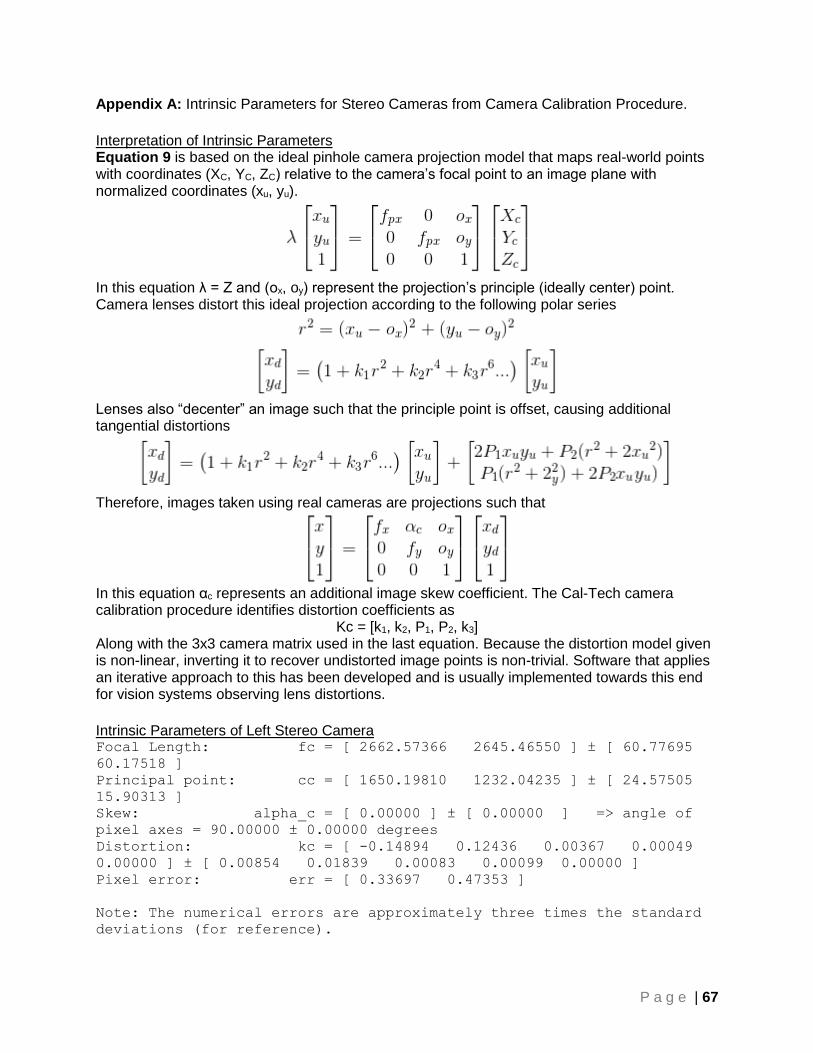
P a g e | 67

Appendix A: Intrinsic Parameters for Stereo Cameras from Camera Calibration Procedure.

Interpretation of Intrinsic Parameters Equation 9 is based on the ideal pinhole camera projection model that maps real-world points with coordinates (XC, YC, ZC) relative to the camera’s focal point to an image plane with normalized coordinates (xu, yu).

In this equation λ = Z and (ox, oy) represent the projection’s principle (ideally center) point. Camera lenses distort this ideal projection according to the following polar series

Lenses also “decenter” an image such that the principle point is offset, causing additional tangential distortions

Therefore, images taken using real cameras are projections such that

In this equation αc represents an additional image skew coefficient. The Cal-Tech camera calibration procedure identifies distortion coefficients as

Kc = [k1, k2, P1, P2, k3] Along with the 3x3 camera matrix used in the last equation. Because the distortion model given is non-linear, inverting it to recover undistorted image points is non-trivial. Software that applies an iterative approach to this has been developed and is usually implemented towards this end for vision systems observing lens distortions.

Intrinsic Parameters of Left Stereo Camera Focal Length: fc = [ 2662.57366 2645.46550 ] ± [ 60.77695

60.17518 ]

Principal point: cc = [ 1650.19810 1232.04235 ] ± [ 24.57505

15.90313 ]

Skew: alpha_c = [ 0.00000 ] ± [ 0.00000 ] => angle of

pixel axes = 90.00000 ± 0.00000 degrees

Distortion: kc = [ -0.14894 0.12436 0.00367 0.00049

0.00000 ] ± [ 0.00854 0.01839 0.00083 0.00099 0.00000 ]

Pixel error: err = [ 0.33697 0.47353 ]

Note: The numerical errors are approximately three times the standard

deviations (for reference).

P a g e | 68

Intrinsic Parameters of Right Stereo Camra Focal Length: fc = [ 2653.89931 2633.30791 ] ± [ 67.20824

67.28770 ]

Principal point: cc = [ 1639.17745 1230.18008 ] ± [ 30.93286

15.11348 ]

Skew: alpha_c = [ 0.00000 ] ± [ 0.00000 ] => angle of

pixel axes = 90.00000 ± 0.00000 degrees

Distortion: kc = [ -0.14784 0.12960 0.00249 -0.00210

0.00000 ] ± [ 0.00930 0.01849 0.00086 0.00128 0.00000 ]

Pixel error: err = [ 0.32013 0.45532 ]

Note: The numerical errors are approximately three times the standard

deviations (for reference).

P a g e | 69

Appendix B: Raw Calibration Point Data

X (ft) Y (ft) Z (ft) x_l y_l x_r y_r

-1.667 1.333 7.5 1721 672 515 694

0 1.333 7.5 2334.5 664.5 1112.5 687.5

1.667 1.333 7.5 2951 661 1715.5 684

-1.667 0 7.5 1721.5 1163.5 520 1178

0 0 7.5 2333 1158 1114.5 1174

1.667 0 7.5 2947.5 1154 1716.5 1171.5

-1.667 -1.333 7.5 1723 1646 525.5 1652

0 -1.333 7.5 2331.5 1642 1118 1651

1.667 -1.333 7.5 2943 1641 1718 1653.5

-3.333 1.333 10 1263.5 803 371 821.5

-1.667 1.333 10 1720 800.5 816.5 819

0 1.333 10 2177.5 796 1264 815

1.667 1.333 10 2637 795 1715 813

3.333 1.333 10 3098 790.5 2171.5 809

-3.333 0 10 1266.5 1169 375.5 1182

-1.667 0 10 1720.5 1168 819 1181

0 0 10 2177 1164 1265 1178

1.667 0 10 2635 1162 1715.5 1177

3.333 0 10 3095.5 1157.5 2170.5 1173.5

-3.333 -1.333 10 1269 1529 380.5 1536

-1.667 -1.333 10 1721 1529 821.5 1537

0 -1.333 10 2176 1526 1266.5 1536

1.667 -1.333 10 2632 1526 1715.5 1538

3.333 -1.333 10 3092.5 1522.5 2170 1536

-5 1.333 12.5 1000 880 292.5 896.5

-3.333 1.333 12.5 1362.5 879 646.5 895

-1.667 1.333 12.5 1728 876 1003.5 892

0 1.333 12.5 2093 872 1362 888

1.667 1.333 12.5 2460 870 1723 886

3.333 1.333 12.5 2828.5 865.5 2087 882

5 1.333 12.5 3197 861.5 2454 879

-5 0 12.5 1004 1172 297 1183

-3.333 0 12.5 1365 1172 650 1184

-1.667 0 12.5 1728.5 1169.5 1005 1182

0 0 12.5 2093 1166 1363 1179

1.667 0 12.5 2459 1163 1724 1177

3.333 0 12.5 2827.5 1159 2088 1173

5 0 12.5 3195.5 1153.5 2453.5 1169.5

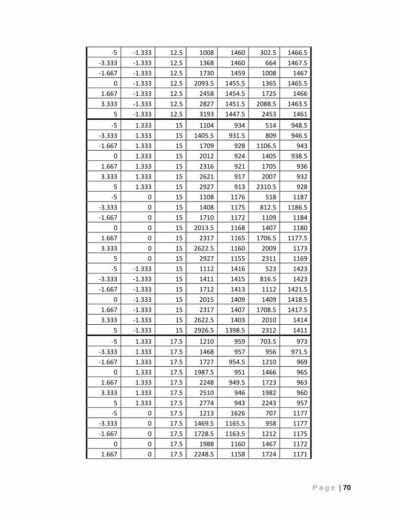
P a g e | 70

-5 -1.333 12.5 1008 1460 302.5 1466.5

-3.333 -1.333 12.5 1368 1460 664 1467.5

-1.667 -1.333 12.5 1730 1459 1008 1467

0 -1.333 12.5 2093.5 1455.5 1365 1465.5

1.667 -1.333 12.5 2458 1454.5 1725 1466

3.333 -1.333 12.5 2827 1451.5 2088.5 1463.5

5 -1.333 12.5 3193 1447.5 2453 1461

-5 1.333 15 1104 934 514 948.5

-3.333 1.333 15 1405.5 931.5 809 946.5

-1.667 1.333 15 1709 928 1106.5 943

0 1.333 15 2012 924 1405 938.5

1.667 1.333 15 2316 921 1705 936

3.333 1.333 15 2621 917 2007 932

5 1.333 15 2927 913 2310.5 928

-5 0 15 1108 1176 518 1187

-3.333 0 15 1408 1175 812.5 1186.5

-1.667 0 15 1710 1172 1109 1184

0 0 15 2013.5 1168 1407 1180

1.667 0 15 2317 1165 1706.5 1177.5

3.333 0 15 2622.5 1160 2009 1173

5 0 15 2927 1155 2311 1169

-5 -1.333 15 1112 1416 523 1423

-3.333 -1.333 15 1411 1415 816.5 1423

-1.667 -1.333 15 1712 1413 1112 1421.5

0 -1.333 15 2015 1409 1409 1418.5

1.667 -1.333 15 2317 1407 1708.5 1417.5

3.333 -1.333 15 2622.5 1403 2010 1414

5 -1.333 15 2926.5 1398.5 2312 1411

-5 1.333 17.5 1210 959 703.5 973

-3.333 1.333 17.5 1468 957 956 971.5

-1.667 1.333 17.5 1727 954.5 1210 969

0 1.333 17.5 1987.5 951 1466 965

1.667 1.333 17.5 2248 949.5 1723 963

3.333 1.333 17.5 2510 946 1982 960

5 1.333 17.5 2774 943 2243 957

-5 0 17.5 1213 1626 707 1177

-3.333 0 17.5 1469.5 1165.5 958 1177

-1.667 0 17.5 1728.5 1163.5 1212 1175

0 0 17.5 1988 1160 1467 1172

1.667 0 17.5 2248.5 1158 1724 1171

P a g e | 71

3.333 0 17.5 2510.5 1154.5 1983 1168

5 0 17.5 2773 1151 2243 1164

-5 -1.333 17.5 1216 1371 710.5 1379

-3.333 -1.333 17.5 1472 1371 961 1379.5

-1.667 -1.333 17.5 1729 1370 1213.5 1379

0 -1.333 17.5 1988 1366 1468 1377

1.667 -1.333 17.5 2248 1366 1725 1376

3.333 -1.333 17.5 2510 1363 1983.5 1374

5 -1.333 17.5 2772 1360 2243.5 1372

-5 1.333 20 1251 1001 806 1014

-3.333 1.333 20 1477.5 1001 1028 1014

-1.667 1.333 20 1704 1000 1251.5 1013

0 1.333 20 1931.5 998 1475.5 1011

1.667 1.333 20 2158 998 1700 1011

3.333 1.333 20 2386 996.5 1926 1010

5 1.333 20 2613.5 995 2152.5 1008.5

-5 0 20 1251.5 1183 806.5 1193

-3.333 0 20 1478 1183 1029 1194

-1.667 0 20 1704 1183 1252 1194

0 0 20 1931 1181 1475.5 1192

1.667 0 20 2158 1180 1700 1192

3.333 0 20 2385.5 1178.5 1926 1190

5 0 20 2613.5 1176.5 2152 1188.5

-5 -1.333 20 1253.5 1362.5 809 1371

-3.333 -1.333 20 1478.5 1363.5 1030 1372

-1.667 -1.333 20 1704.5 1363 1252 1372

0 -1.333 20 1931 1361.5 1476 1371

1.667 -1.333 20 2158 1361 1700 1371

3.333 -1.333 20 2385.5 1360 1926 1370.5

5 -1.333 20 2612.5 1358.5 2151.5 1369.5

-0.5625 0.520833 5 2352 950 523.5 969.5

-0.1875 0.520833 5 2558.5 948 724 968.5

0.1875 0.520833 5 2766 946 925.5 966.5

0.520833 0.520833 5 2971 944 1125 965

-0.5625 0 5 2351.5 1259 530 1273

-0.1875 0 5 2557.5 1258 730 1273

0.1875 0 5 2763.5 1257 930 1272

0.520833 0 5 2968 1255 1129.5 1271.5

-0.5625 -0.52083 5 2350.5 1567 535 1575.5

-0.1875 -0.52083 5 2555 1566 734 1575.5

P a g e | 72

0.1875 -0.52083 5 2761 1565 934 1575

0.520833 -0.52083 5 2964.5 1563.5 1132.5 1575.5

25 1215 988 858 1000

25 1217 1175 861.5 1185.5

25 1219 1364 863.5 1371.5

25 1429.5 987.5 1069.5 999.5

25 1430.5 1175.5 1071 1185

25 1432 1364 1073.5 1371.5

25 1643 987 1280.5 999.5

25 1645 1175 1282 1185

25 1646 1364 1285 1372

25 1858 986 1493 998

25 1859 1175 1494.5 1198.5

25 1859.5 1363.5 1495.5 1371.5

25 2072 987 1705 998

25 2073 1174 1706 1184

25 2073.5 1362.5 1706.7 1371.5

25 2286 986 1917 997

25 2286.5 1174.5 1918.5 1184.5

25 2286.2 1362.5 1919 1371

25 2500.5 985.5 2131 996

25 2499.5 1173.5 2131.5 1183.5

25 2499.5 1361.5 2131 1371

30 1277 1005 977 1016

30 1278 1162 979.5 1170.5

30 1279.5 1318.5 981 1326

30 1456 1005 1154 1015

30 1456.5 1161.5 1155 1170

30 1458 1319 1157 1326

30 1634 1005 1329.5 1015.5

30 1635.5 1161.5 1332 1170

30 1636 1319 1333 1326

30 1813 1004 1507.5 1014.5

30 1814 1162 1508 1170

30 1814.5 1318.5 1509.5 1325.5

30 1990.5 1005.5 1684.5 1014.5

30 1992.5 1161.5 1685 1170

30 1992 1318 1686 1326

30 2168.5 1004.5 1861 1014

30 2169 1161 1862 1170

P a g e | 73

30 2169 1318 1862 1326

30 2347 1004 2038 1014

30 2346.5 1160.5 2038.5 1169.5

30 2346 1318 2038.5 1325.5

P a g e | 74

Appendix C: Source Code for System User Interface Headings reflect file location relative to document root /var/www

/index.html <!DOCTYPE html>

<html>

<head>

<link rel="stylesheet" type="text/css" href="interfaceStyles.css">

<style>

img:hover {

border: 3px solid #777;

}

</style>

<title>System Home</title>

<script>

var targetsQuery = new XMLHttpRequest();

window.onload = function() {

targetsQuery.open("GET", "TargetCounts.php");

targetsQuery.send();

};

function CameraInit() {

var initRequest = new XMLHttpRequest();

initRequest.open("GET", "/cgi-bin/CameraInit.sh");

initRequest.send();

}

</script>

</head>

<body>

<h1>Stereo Vision Ranging System - Main Interface</h1>

<h2>Overview</h2>

<p>This site acts as the user interface for a stereo vision system

created to determine the position of target objects

relative to it. Users are able to mark targets by drawing rectangles

around them within

stereo image sets. The abbreviated list below gives instructions on

how to operate this system using its interface.</p>

<h2>Procedure for Range Measurements</h2>

<ol>

<li>When both cameras are first activated, their lenses may be

retracted.<br>

If this is the case, press the 'Initialize' button below to set

up the cameras for image collection.</li>

<li>Point the system cameras in the direction of the desired target

object(s).</li>

<li>Retrieve a stereo image set from the cameras by pressing the

"Capture" button.</li>

<li>From this page, click on one of the images displayed below to

open a target identification dialogue.</li>

<li>Once targets have been found, click the "Process" button to view

range and position estimates for identified targets.</li>

P a g e | 75

</ol>

<div align="center">

Camera Units: <button class="button"

onclick="CameraInit()">Initialize</button>

</div>

<table align="center" style="margin-top: 12px">

<tr>

<td align="center">

<button class="button" onclick="window.location.href='/cgi-

bin/CameraTrigger.html'">Capture</button>

</td>

<td align="center">

<span id="lblConjError" style="display: none; color: yellow">

Error: left and right images have different numbers of

marked targets.

</span>

<button id="btnProcess" class="button" style="display: none"

onclick="window.location.href='/ResultsPlot/index.php'">

Process

</button>

</td>

</tr>

<tr>



<td>

<a href="./UserTargeting/index.html?position=left">

<div id="left_cell" style="width: 600px; height: 400px;

background-color: white">

<img id="left_preview" src="/ImageSet/Left_Image.jpg"

alt="Failed to load Left Image" width="600" height="400">

</div>

</a>

</td>

<td>

<a href="./UserTargeting/index.html?position=right">

<div id="right_cell" style="width: 600px; height: 400px;

background-color: white">

<img id="right_preview"

src="/ImageSet/Right_Image.jpg" alt="Failed to load Right Image" width="600"

height="400">

</div>

</a>

</td>

</tr>

<tr>

<td align="center">

<p><span id="LeftCount">0</span> Targets selected in

left image</p>

</td>

<td align="center">

<p><span id="RightCount">0</span> Targets selected in

left image</p>

</td>

</tr>

</table>

<script>

P a g e | 76

targetsQuery.onreadystatechange = function() {

if (targetsQuery.readyState === 4 && targetsQuery.status === 200)

{

var rData = targetsQuery.responseText;

var values = rData.split(',');

if (values.length > 1)

{

document.getElementById("LeftCount").innerHTML =

values[0];

document.getElementById("RightCount").innerHTML =

values[1];

if (values[0] > 0 || values[1] > 0) // both images have

marked targets

{

if (values[0] === values[1]) // all marks have

conjugates in other image

{

document.getElementById("btnProcess").style.display = "inline";

}

else // inform the user otherwise

{

document.getElementById("lblConjError").style.display = "inline";

}

}

}

else

{

console.log("Exit" + rData);

}

}

};

</script>

</body>

</html>

/interfaceStyles.css .button {

padding: 15px 25px;

margin: 10px 10px 10px 10px;

font-size: 24px;

text-align: center;

cursor: pointer;

outline: none;

color: #000;

background-color: lightgrey;

border: none;

border-radius: 15px;

box-shadow: 0 4px #999;

}

.button:hover {background-color: darkgrey}

.button:active {

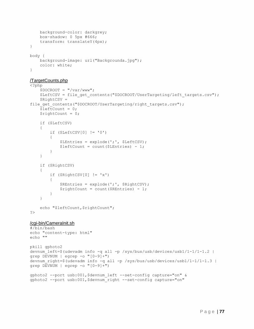
P a g e | 77

background-color: darkgrey;

box-shadow: 0 5px #666;

transform: translateY(4px);

}

body {

background-image: url("Backgrounda.jpg");

color: white;

}

/TargetCounts.php <?php

$DOCROOT = "/var/www";

$LeftCSV = file_get_contents("$DOCROOT/UserTargeting/left_targets.csv");

$RightCSV =

file_get_contents("$DOCROOT/UserTargeting/right_targets.csv");

$leftCount = 0;

$rightCount = 0;

if ($LeftCSV)

{

if ($LeftCSV[0] != '0')

{

$LEntries = explode(';', $LeftCSV);

$leftCount = count($LEntries) - 1;

}

}

if ($RightCSV)

{

if ($RightCSV[0] != 'x')

{

$REntries = explode(';', $RightCSV);

$rightCount = count($REntries) - 1;

}

}

echo "$leftCount,$rightCount";

?>

/cgi-bin/CameraInit.sh #/bin/bash

echo "content-type: html"

echo ""

pkill gphoto2

devnum_left=$(udevadm info -q all -p /sys/bus/usb/devices/usb1/1-1/1-1.2 |

grep DEVNUM | egrep -o "[0-9]+")

devnum_right=$(udevadm info -q all -p /sys/bus/usb/devices/usb1/1-1/1-1.3 |

grep DEVNUM | egrep -o "[0-9]+")

gphoto2 --port usb:001,$devnum_left --set-config capture="on" &

gphoto2 --port usb:001,$devnum_right --set-config capture="on"

P a g e | 78

/cgi-bin/CameraTrigger.html <!DOCTYPE html>

<html>

<head>

<link rel="stylesheet" type="text/css" href="/interfaceStyles.css">

<title>Capture Trigger</title>

<script>

var captureRequest = new XMLHttpRequest();

captureRequest.open("GET", "CameraTrigger.sh");

captureRequest.onreadystatechange = function() {

var response;

if (captureRequest.readyState === 4 && captureRequest.status

=== 200)

{

response = captureRequest.responseText;

if (response[0] === "1") // if not exit 0

{

alert("An error was encountered while retirieving the

stereo image set. Refresh this page to try again");

}

else

{

window.location.href = "/index.html";

}

}

};


captureRequest.send();

setTimeout(function()

{document.getElementById("waitPrompt").innerHTML = "Images Captured,

Downolading...";}, 5000);

};

</script>

</head>

<body>

<h1>Processing Request</h1>

<p>This page will automatically return to System Home after image

capture is complete.</p>

<h2>Triggering Cameras...</h2>

<h2 id="waitPrompt"></h2>

</body>

</html>

/cgi-bin/CameraTrigger.sh #!/bin/bash

echo "Content-type: text/html"

echo ""

DOCROOT="/var/www"

rm $DOCROOT/ImageSet/*_Image.jpg

printf "x" > $DOCROOT/UserTargeting/left_targets.csv

printf "x" > $DOCROOT/UserTargeting/right_targets.csv

# Make sure LeftCam.sh and RightCam.sh trigger scripts are

# in same directory

P a g e | 79

sh ./LeftCam.sh & sh ./RightCam.sh &

COUNTER=0

ECODE=1

# give the images 15 seconds to process, then exit from script

while [ $COUNTER -lt 15 ]

do

if [ -e $DOCROOT/ImageSet/Left_Image.jpg -a -e

$DOCROOT/ImageSet/Right_Image.jpg ]

then

ECODE=0 #exit 0

break

fi

COUNTER=$(($COUNTER + 1))

sleep 1

done

echo "$ECODE;$COUNTER"

/UserTargeting/index.html <!DOCTYPE html>

<head>



<link rel="stylesheet" type="text/css" href="../interfaceStyles.css">

<style>

.edgeInput {

width: 60px;

padding-left: 6px;

font-size: 18px;

}

#TargetEditor {

z-index: 3;

position: absolute;

left: -200px;

width: 150px;

background-color: #F0F0F0;

border-style: solid;

border-width: 1px;

padding: 12px 12px 12px 12px;

font-size: 18px;

color: black;

}

</style>

<title>User Targeting</title>

<script>


// dynamically load image from GET query

var qGET = new RegExp("position=(left|right)");

var argv = qGET.exec(window.location.search);

if (argv)

{

if (argv[0] === "position=left")

{

document.getElementById("WorkingImage").src =

"../ImageSet/Left_Image.jpg";

P a g e | 80

Camera_Shown = "left";

}

else if (argv[0] === "position=right")

{

document.getElementById("WorkingImage").src =

"../ImageSet/Right_Image.jpg";

Camera_Shown = "right";

}

}

// AJAX call to load defined rectangles

if (Camera_Shown === "left")

{

loadRequest.send("filename=/UserTargeting/left_targets.csv");

}

else if (Camera_Shown === "right")

{

loadRequest.send("filename=/UserTargeting/right_targets.csv");

}

};

/* External call to load and paint rectangles previously marked on image

*/

var loadRequest = new XMLHttpRequest();

loadRequest.open("POST", "/cgi-bin/ImportCSV.php", true);

// Required to pass POST data from js

loadRequest.setRequestHeader("Content-type", "application/x-www-form-

urlencoded");

loadRequest.onreadystatechange = function() {

if (loadRequest.readyState === 4 && loadRequest.status === 200)

{

var rData = loadRequest.responseText;

var entries = rData.split(';');

var i;

for (i=0; i<entries.length; i++)

{

var rectArgs = entries[i].split(',');

if (rectArgs.length === 4)

{

// load archived rectangle data into array

var objRectangle = new

Rectangle(parseInt(rectArgs[0]*ImageScale), parseInt(rectArgs[1]*ImageScale),

parseInt(rectArgs[2]*ImageScale),

parseInt(rectArgs[3]*ImageScale));

Rects.push(objRectangle);

// paint loaded rectangle

drawing_context.beginPath();

drawing_context.strokeStyle = "red";

drawing_context.strokeRect(objRectangle.x,

objRectangle.y, objRectangle.w, objRectangle.h);

}

}

}

};

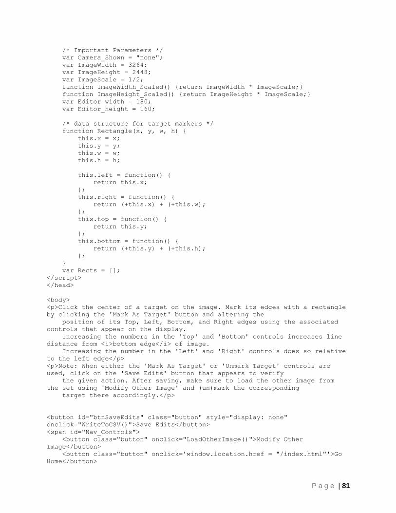
P a g e | 81

/* Important Parameters */

var Camera_Shown = "none";

var ImageWidth = 3264;

var ImageHeight = 2448;

var ImageScale = 1/2;

function ImageWidth_Scaled() {return ImageWidth * ImageScale;}

function ImageHeight_Scaled() {return ImageHeight * ImageScale;}

var Editor_width = 180;

var Editor_height = 160;

/* data structure for target markers */

function Rectangle(x, y, w, h) {

this.x = x;

this.y = y;

this.w = w;

this.h = h;

this.left = function() {

return this.x;

};

this.right = function() {

return (+this.x) + (+this.w);

};

this.top = function() {

return this.y;

};

this.bottom = function() {

return (+this.y) + (+this.h);

};

}

var Rects = [];

</script>

</head>

<body>

<p>Click the center of a target on the image. Mark its edges with a rectangle

by clicking the 'Mark As Target' button and altering the

position of its Top, Left, Bottom, and Right edges using the associated

controls that appear on the display.

Increasing the numbers in the 'Top' and 'Bottom' controls increases line

distance from <i>bottom edge</i> of image.

Increasing the number in the 'Left' and 'Right' controls does so relative

to the left edge</p>

<p>Note: When either the 'Mark As Target' or 'Unmark Target' controls are

used, click on the 'Save Edits' button that appears to verify

the given action. After saving, make sure to load the other image from

the set using 'Modify Other Image' and (un)mark the corresponding

target there accordingly.</p>

<button id="btnSaveEdits" class="button" style="display: none"

onclick="WriteToCSV()">Save Edits</button>

<span id="Nav_Controls">

<button class="button" onclick="LoadOtherImage()">Modify Other

Image</button>

<button class="button" onclick='window.location.href = "/index.html"'>Go

Home</button>

P a g e | 82

</span>

<div>

<button id="btnAddMark" class="button" onclick="AddNewRect()">Mark as

Target</button>

<button id="btnRemMark" class="button"

onclick="DeleteCurrentRect()">Unmark Target</button>

</div>

<div id="Targeting_Markup" style="position:relative; width:1650px;

height:1250px">



<script>

/* ---------- Implementation Variables ---------- */

// references for drawing target markers

var drawing_context =

document.getElementById("MarkupCanvas").getContext("2d");

drawing_context.lineWidth="1";

drawing_context.fillStyle="cyan";

var RectIndex = -1; // Index of current working rectangle. Reset to -1

when none selected

// numeric variables for cursor position (determined when image display

is clicked)

var intCx = 0;

var intCy = 0;

var cursorLock = false;

/* ---------- Input Handler Functions ---------- */

P a g e | 83

function LoadOtherImage() {

var reURL = "./index.html?position=";

if (Camera_Shown === "left")

{

reURL += "right";

}

else if (Camera_Shown === "right")

{

reURL += "left";

}

console.log("Redirecting to " + reURL);

window.location.href = reURL;

}

function WriteToCSV() {

if (Camera_Shown !== "none")

{

// ATF 2016-02-22: prep export string client side

var saveRequest = new XMLHttpRequest();

var fname = "/UserTargeting/" + Camera_Shown + "_targets.csv";

var ArrayString = "";

if (Rects.length > 0)

{

for (var i=0; i<Rects.length; i++)

{

ArrayString += parseInt(Rects[i].x/ImageScale) + ',' +

parseInt(Rects[i].y/ImageScale) + ',' + parseInt(Rects[i].w/ImageScale) + ','

+ parseInt(Rects[i].h/ImageScale) + ';';

}

}

else

{

ArrayString = "x";

}

saveRequest.open("POST", "/cgi-bin/ExportCSV.php", true);

// Required to pass POST data from js

saveRequest.setRequestHeader("Content-type", "application/x-www-

form-urlencoded");

saveRequest.send("filename=" + fname + "&data=" + ArrayString);

}

else

{

console.log("No image was loaded when save request submitted");

}

// show navigation controls

document.getElementById("Nav_Controls").style.display = "inline";

// hide save button

document.getElementById("btnSaveEdits").style.display = "none";

// hide delete marker button

document.getElementById("btnRemMark").style.display = "none";

}

/* Handles click event on image canvas */

P a g e | 84

document.getElementById("MarkupCanvas").onmousedown = function (event) {

var offsetRect = this.getBoundingClientRect();

var index;

var item;

if (!cursorLock)

{

// if no target is selected, erase old cursor position

if (RectIndex<0)

{


drawing_context.clearRect(intCx-4, intCy-4, 9, 9);

}

// get mouse click coordinates for cursor

intCx = event.x - offsetRect.left;

intCy = event.y - offsetRect.top;

// search Rects array to see if an existing one is being selected

for (index=0; index<Rects.length; index++)

{

item = Rects[index];

if ((intCx > item.left()) && (intCx < item.right()) && (intCy

> item.top()) && (intCy < item.bottom()))

{

break;

}

}

if (index < Rects.length) // existing rectangle has been clicked,

select it

{

if (index!==RectIndex)

{

// recolor rectangle that was selected before function

call

if (RectIndex >= 0)

{

drawing_context.strokeStyle="red";

DrawRect(Rects[RectIndex]);

}

RectIndex = index; // change current working rectangle

drawing_context.strokeStyle="cyan";

DrawRect(item);

// hide add control

document.getElementById("btnAddMark").style.display =

"none";

// update the values in the input controls for current

selection

document.getElementById("CurrentTop").value =

ImageHeight_Scaled() - item.top();

document.getElementById("CurrentLeft").value =

item.left();

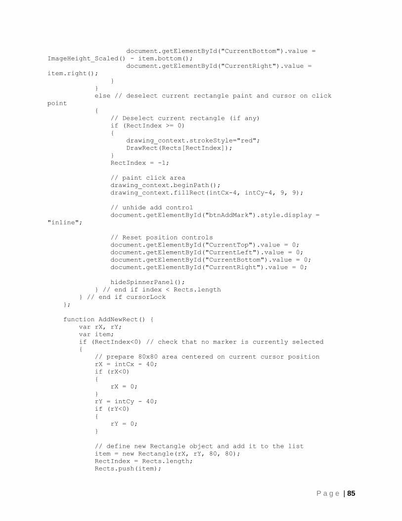
P a g e | 85

document.getElementById("CurrentBottom").value =

ImageHeight_Scaled() - item.bottom();

document.getElementById("CurrentRight").value =

item.right();

}

}

else // deselect current rectangle paint and cursor on click

point

{

// Deselect current rectangle (if any)

if (RectIndex >= 0)

{

drawing_context.strokeStyle="red";

DrawRect(Rects[RectIndex]);

}

RectIndex = -1;

// paint click area


drawing_context.fillRect(intCx-4, intCy-4, 9, 9);

// unhide add control


"inline";

// Reset position controls

document.getElementById("CurrentTop").value = 0;

document.getElementById("CurrentLeft").value = 0;

document.getElementById("CurrentBottom").value = 0;

document.getElementById("CurrentRight").value = 0;

hideSpinnerPanel();

} // end if index < Rects.length

} // end if cursorLock

};

function AddNewRect() {

var rX, rY;

var item;

if (RectIndex<0) // check that no marker is currently selected

{

// prepare 80x80 area centered on current cursor position

rX = intCx - 40;

if (rX<0)

{

rX = 0;

}

rY = intCy - 40;

if (rY<0)

{

rY = 0;

}

// define new Rectangle object and add it to the list

item = new Rectangle(rX, rY, 80, 80);

RectIndex = Rects.length;

Rects.push(item);

P a g e | 86

// clear rectangle area for repaint



drawing_context.clearRect(item.x - 2, item.y - 2, item.w + 4,

item.h + 4);

// overlay it on the image

DrawRect(item);

// update the values in the input controls for current selection

document.getElementById("CurrentTop").value =

parseInt(ImageHeight_Scaled() - item.top());

document.getElementById("CurrentLeft").value =

parseInt(item.left());

document.getElementById("CurrentBottom").value =

parseInt(ImageHeight_Scaled() - item.bottom());

document.getElementById("CurrentRight").value =

parseInt(item.right());

// hide control for adding targets

cursorLock = true;

//document.getElementById("Add_Del_Controls").style.display =

"none";

document.getElementById("btnAddMark").style.display = "none";

// hide navigation controls

document.getElementById("Nav_Controls").style.display = "none";

// show save button

document.getElementById("btnSaveEdits").style.display = "inline";

}

}

function ChangeCurrentRect() {

var item;

if (RectIndex>=0)

{

item = Rects[RectIndex];

// clear rectangle area for repaint




item.h + 4);

// get its information from editor

item.x = document.getElementById("CurrentLeft").value;

item.y = ImageHeight_Scaled() -

document.getElementById("CurrentTop").value;

item.w = document.getElementById("CurrentRight").value - item.x;

item.h = (ImageHeight_Scaled() -

document.getElementById("CurrentBottom").value) - item.y;

Rects[RectIndex] = item;

DrawRect(item);


document.getElementById("Nav_Controls").style.display = "none";

// show save button

P a g e | 87

document.getElementById("btnSaveEdits").style.display = "inline";

}

}

function DeleteCurrentRect() {

var item;

if (RectIndex>=0)

{

// Get working item from the Rects array

item = Rects[RectIndex];

Rects.splice(RectIndex, 1); // remove it from the array

RectIndex = -1;

// clear it from the display



item.h + 4); // erase current rectangle

// Reset position controls

document.getElementById("CurrentTop").value = 0;

document.getElementById("CurrentLeft").value = 0;

document.getElementById("CurrentBottom").value = 0;

document.getElementById("CurrentRight").value = 0;

// Hide panel

hideSpinnerPanel();

if (!cursorLock) // unmarking existing rectangle: hide add_del

buttons

{

document.getElementById("btnAddMark").style.display = "none";

document.getElementById("btnRemMark").style.display = "none";


document.getElementById("Nav_Controls").style.display =

"none";

// show save button

document.getElementById("btnSaveEdits").style.display =

"inline";

}

else // unmarking rectangle just added, restore add button

{


"inline";

// show navigation controls

document.getElementById("Nav_Controls").style.display =

"inline";

// hide save button

document.getElementById("btnSaveEdits").style.display =

"none";

}

cursorLock = !cursorLock;

}

}

/* ---------- Helper methods for input responses ---------- */

P a g e | 88

/* Overlays outline of the input rectangle on image using the current

stroke color */

function DrawRect(objRectangle) {

//var item;

var editorX, editorY;

// paint input rectangle


drawing_context.strokeRect(objRectangle.x, objRectangle.y,

objRectangle.w, objRectangle.h);

// position spinner panel next to active rectangle

if (objRectangle.x > Editor_width)

{

editorX = objRectangle.x - Editor_width - 10;

}

else

{

editorX = objRectangle.right() + 10;

}

if (objRectangle.y < (ImageHeight_Scaled() - Editor_height))

{

editorY = objRectangle.y - 10;

}

else

{

editorY = ImageHeight_Scaled() - Editor_height;

}

showSpinnerPanel(editorX, editorY);

}

/* Moves the top left or right corner of teh SpinnerPanel to the

coordinates input */

function showSpinnerPanel(x, y) {

var SpinnerPanel1 = document.getElementById("TargetEditor");

SpinnerPanel1.style.left = x + "px";

SpinnerPanel1.style.top = y + "px";

}

function hideSpinnerPanel() {

document.getElementById("TargetEditor").style.left = "-200px";

}

</script>

</body>

</html>

/cgi-bin/ImportCSV.php <?php

// script takes 1 external inputs: filename for csv data

$fname = htmlspecialchars($_POST['filename']);


if ($fname)

{

if ($fname[0] == '/') // relative path passed from javascript, prepend

actual server path

P a g e | 89

{

$fname = $DOCROOT . $fname;

}

$fdata = file_get_contents($fname);

if ($fdata)

{

echo "$fdata";

}

}

?>

/cgi-bin/ExportCSV.php <?php

// script takes 2 external inputs: filename and data strings

$fname = htmlspecialchars($_POST['filename']);

$fdata = htmlspecialchars($_POST['data']);


$ecode = 1;

if ($fname)

{

if ($fname[0] == '/') // relative path passed from javascript, prepend

actual server path

{

$fname = $DOCROOT . $fname;

}

if ($fname && $fdata)

{

file_put_contents($fname, $fdata);

$ecode = 0;

}

}

echo "$ecode";

?>

/ResultsPlot/index.php <!DOCTYPE html>



<html>

<head>

<link rel="stylesheet" type="text/css" href="../interfaceStyles.css">

<title>Target Locations</title>

<script src="Chart.js"></script>

<script src="Chart.Scatter.js"></script>

<style>

.container {

margin-left: 10%;

margin-right: 10%;

margin-bottom: 5%;

P a g e | 90

}

#myChartArea {

background-color: white;

border: 1px solid #777;

}

</style>

<?php

$DOCROOT="/var/www";

$left_csv = exec("./CPointUndistort CalibData_Left.dat

$DOCROOT/UserTargeting/left_targets.csv");

$right_csv = exec("./CPointUndistort CalibData_Right.dat

$DOCROOT/UserTargeting/right_targets.csv");

?>

</head>

<body>

<div style="margin-bottom: 12px">

<button class="button"

onclick="window.location.href='/index.html'">Home</button>

<h1 style="display: inline; margin-left: 12px">Locations of Marked

Targets: (X, Z) [feet]</h1>

</div>

<div class="container">

<canvas id="myChartArea" width="800" height="600"></canvas>

</<div>

<script>

//Create the chart

var ctx = document.getElementById("myChartArea").getContext("2d");

var myChart = new Chart(ctx);

var data = [

{

label: 'Target Location',

strokeColor: '#007ACC',

pointColor: '#007ACC',

pointStrokeColor: '#fff',

data: [

<?php

if ($left_csv && $right_csv)

{

$left_markers = explode(';', $left_csv);

$right_markers = explode(';', $right_csv);

$leftCount = count($right_markers);

$rightCount = count($left_markers);

// filter out characters trailing last ';' (\n,

fragments)

$last = explode(',', $left_markers[$leftCount - 1]);

if (count($last != 2))

{

$leftCount -= 1;

}

$last = explode(',', $right_markers[$rightCount -

1]);

if (count($last != 2))

P a g e | 91

{

$rightCount -= 1;

}

/* Parameters (calculated in MatLab based on

experimental data) */

// Z = K_Bf * d^A; // ideally A = -1, but this may

not be the case with experimental data sets

$K_Bf = 9025.254513491886;

$A = -0.998730743735693;

// xbar = f(X/Z) + P

$fx = 2723.051556332627;

$P = 1716.506479025595;

// angle (cw) between plane and relative X axis

(based on average model reprojection errors)

$planeSlope = 0.067958;

// X (centered on B/2) = (B/2)(1 - (2 * x_l - x_o)/d)

if ($leftCount == $rightCount) // same number of

targets marked in both images -> plot ranges

{

for ($i=0; $i < $leftCount; $i++)

{

// find disparity based on center of target

rectangles

$leftRect = explode(',', $left_markers[$i]);

$left_center = floatval($leftRect[0]); //

undistorted X_l

$rightRect = explode(',',

$right_markers[$i]);

$right_center = floatval($rightRect[0]); //

undistorted X_r

$d = abs($left_center - $right_center);

$xbar = 0.5*($left_center + $right_center);

// recover Z using calibration model

$Z = $K_Bf*pow($d, $A);

// recover X using Z

$X = $Z*($xbar - $P)/$fx ;

// adjust Z to account for reprojection skew

$Z += $X*$planeSlope;

printf("{ x: %.2f, y: %.2f, r: 2 }", $X, $Z);

if ($i < $leftCount)

{

echo ',';

}

}

}

}

?>

]

},

{

label: 'X-Scale',

pointColor: '#fff',

data: [

P a g e | 92

{ x: -25, y: 0, r: 0.01 },

{ x: 25, y: 0, r: 0.01 }

]

}

];


myChart.Scatter(data, {responsive: true, animation: true,

datasetStroke: false, scaleBeginAtZero: true});

};

</script>

</body>

</html>

/ResultsPlot/CPointUndistort

/*

* To change this license header, choose License Headers in Project

Properties.

* To change this template file, choose Tools | Templates

* and open the template in the editor.

*/

/*

* File: main.cpp

* Author: pi

*

* Created on February 29, 2016, 8:37 AM

*/

#include <opencv2/opencv.hpp>

#include <iostream>

#include <cstring>

#include <fstream>

#include <vector>

#define MATFILE_EXT ".dat"

#define POINTFILE_EXT ".csv"

using namespace std;

struct Rectangle {

unsigned int x, y, w, h;

};

/* Inputs:

* [0] string name of the xml file containing camera matrix and distortion

coefficients matrix

* [1] string name of the csv file containing target rectangle data

*/

int main(int argc, char** argv)

{

if (argc < 3 ) // check for valic argument count

{

return -1;

P a g e | 93

}

if ( !(strstr(argv[1], MATFILE_EXT) && strstr(argv[2], POINTFILE_EXT)) )

// check for valid input file extensions

{

return -1;

}

using namespace cv;

int i;

bool rError = true;

std::ifstream calParamFile(argv[1]);

Mat cameraMatrix(3,3,CV_64F);

Mat distCoeff(1,5,CV_64F);

std::ifstream targetsCSV(argv[2]);

struct Rectangle userMark;

Point2d cp;

std::vector<Point2d> points;

Mat dst;

double *dptr;

if (calParamFile.good() && targetsCSV.good())

{

calParamFile.ignore(1024, '\n'); // ignore header1

dptr = (double *)cameraMatrix.data; // get Camera matrix

i = 0;

while (calParamFile.good())

{

calParamFile >> dptr[i];

calParamFile.ignore(1);

if (++i >= 9 || calParamFile.eof())

{

break;

}

}

rError = (i < 9); // error reading camera matrix

calParamFile.ignore(1024, '\n'); // finish line read

calParamFile.ignore(1024, '\n'); // ignore header2

dptr = (double *)distCoeff.data; // get distortion coefficient vector

i = 0;

while (calParamFile.good())

{

calParamFile >> dptr[i];

calParamFile.ignore(1);

if (++i >= 5 || calParamFile.eof())

{

break;

}

}

rError = (i < 5);

calParamFile.close();

while (targetsCSV.good()) // read marked target data

{

P a g e | 94

targetsCSV >> userMark.x;

targetsCSV.ignore(1);

targetsCSV >> userMark.y;


targetsCSV >> userMark.w;


targetsCSV >> userMark.h;


if (targetsCSV.eof())

{

break;

}

cp.x = userMark.x + userMark.w/2;

cp.y = userMark.y + userMark.h/2;

points.push_back(cp);

}

targetsCSV.close();

if (!rError)

{

// undistort selected points

undistortPoints(points, dst, cameraMatrix, distCoeff, noArray(),

cameraMatrix);

// print the results

std::cout.precision(15);

dptr = (double *)dst.data;

for (i=0; i<dst.cols; i++)

{

cp.x = *(dptr + i * 2);

cp.y = *(dptr + i * 2 + 1);

std::cout << cp.x << ',' << cp.y << ';';

}

return 0;

}

else

{

return 1;

}

}

else

{

return 1;

}

}

Indiana University-Purdue University Fort Wayne ECE 406 ...

Documents

Transcript of Indiana University-Purdue University Fort Wayne ECE 406 ...