Index Terms IJSER · · 2016-10-02ern part of the Bay of Bengal, ... intensity estimates used for...

International Journal of Scientific & Engineering Research, Volume 7, Issue 9, September-2016 437 ISSN 2229-5518

IJSER © 2016 http://www.ijser.org

Intensity Analysis of Tropical Cyclone using Dvorak Technique

Md.Rubyet Kabir, Md. Abdur Rahman Khan, Md. Rashaduzzaman, S.M. Quamrul Hasan

Abstract— The tropical warm Indian Ocean, like the tropical North Atlantic, the South Pacific and the NE Pacific, is a breeding ground for the disastrous tropical cyclone (TC) phenomenon. TCs are accompanied by very strong winds, torrential rains and storm surges. Historically, in terms of loss to human life, the Bay of Bengal TCs have accounted for deaths ranging from a thousand to three hundred thousand. It is now a well known fact of climatology that about 5 to 6 TCs occur in the Bay of Bengal prominently during the pre-monsoon season (March-April-May) and the post-monsoon season (October-November-December).Nearly 5 percent of the global TCs form in the Bay of Bengal. The maximum frequency is in the two months of May and November. This paper contains descriptions of designed to be used with visible, enhanced infrared and digital infrared data. The analysis techniques all use cloud feature measurements and rules based on a model of tropical development to arrive at the current and future intensity of a tropical cyclone. The model describes tropical cyclone development in terms of day by day changes in the cloud pattern of the storm and its environment.The enhanced and digital infrared techniques, when applied to storms of cyclone strength, rely almost entirely on measurements of the “eye” temperature and the temperature of the clouds around the eye for the intensity determination.When visual pictures, or infrared pictures of weaker disturbances, are used for the intensity analysis the cloud feature measurements are usually more subjective and more complex. The analysis involves the appearance of the clouds forming the cloud system center and those encircling the center as well as measurements of these features. Methods used to forecast tropical cyclone development and weakening and also include a recently developed technique that uses cloud feature indications of changes in the westerly jet stream to forecast changes in tropical cyclone intensity.

Index Terms— Dvorak Technique, T-number, Cyclone–intensity, Satellites, Visibel and Infrared, Tropical Cyclone.

—————————— ——————————

1 INTRODUCTION

HE Dvorak (1984) technique analysis is the worldwide standard for tropical cyclone intensity monitoring and used in identification of clouds types, pattern, clouds top

height and temperature. The absence of aircraft reconnais-sance it is the most common method of intensity forecasting as well. It can also be used for monitor flood and rainfall clouds pattern. The advanced Dvorak technique (ADT; Olander and Velden 2007), which already uses modified pressure–wind relationships developed by Kossin and Velden (2004) based on Atlantic aircraft data. The most influential data source for es-timating tropical cyclone intensity and position is aircraft re-connaissance. However in most tropical cyclone basins and a majority of the time, such observations are unavailable. When this situation occurs, the Dvorak Technique (DVKT) is the most widely available and readily used tool for operationally estimating the maximum wind speeds associated with tropical cyclones. BMD can use these relationships for Bay of Bengal region. Now, BMD using SATAID (Himawari), INSAT and CY-2 satellite imageries and others software for tropical cyclone

forecast. NWP model and ensemble method also used in de-tection of cyclone track prediction and different types of guid-ance for good accuracy of cyclone forecast. It also used in identification of clouds types, pattern, clouds top height and temperature. The tropical cyclone is an atmospheric pheno-menon with strong low pressure areas of horizontal dimen-sion of around 500-1000 km and with central pressure drop ranging from 6-64 hPa and wind speed ranges from 62kph to around 250kph or more.The tropical cyclone is the strongest and most disastrous meteorological phenomena of the tropics that from over the tropical warm tropical oceans with temper-ature above 26.5C within the 50 metre the depth of the thermo cline. Tropical cyclones have well defined core structure of radius 100-200km.

T

———————————————— • Md.Rubyet Kabir is currently pursuing as a Meteorologist in Bangladesh

Meteorological Department, Bangladesh, PH-+88 02 9135742. E-mail: [email protected] Md.

• Abdur Rahman Khan is currently pursuing as a Meteorologist in Bangla-desh Meteorological Department, Bangladesh, PH-+88 02 9135742.. E-mail: [email protected]

• Md. Rashaduzzaman is currently pursuing as a Meteorologist in Bangla-desh Meteorological Department, Bangladesh, PH-+88 02 9135742.E-mail [email protected]

• S. M. Quamrul Hasan is currently pursuing as a Meteorologist in Bangla-desh Meteorological Department, Bangladesh, PH-+88 02 9135742.. E-mail: [email protected]

Fig. 1. Tracks of cyclones over the north Indian Ocean during 1891-2007 (Source IMD)

IJSER

http://www.ijser.org/



Tropical cyclone 1991 was a category 5 cyclone which made landfall in Bangladesh on April 29, 1991, causing a storm surge of up to 10m across much of the country. It was one of the worst natural disasters to occur in Bangladesh, with estimates of up to 190000 deaths. Cyclone 1991 developed in the south-ern part of the Bay of Bengal, close to the Andaman Islands. In developed and strengthened as it moved North-East. By the time of landfall at Bangladesh (89.8 E) on April 29th, the sus-tained winds were around 215 km/hr. After landfall, the storm dissipated rapidly.

The area of landfall was on the estern coast of Bangladesh.

It is the populated area of the country, as it is home to the Chittagong. At the point of landfall, storm surges of up to 25 feet are possible. Meanwhile, storm surges of between 10 to 20 feet are also likely to affect populated areas.

Bangladesh Meteorological Department reported that Cyc-lone 1991 brought winds of 160 to 180 kph (100 to 11 mph) to Chittagong, Hatia, Khepupara and Dublarchar coastlines at about 5:00 p.m. local time. The Meteorology Office warned that the coastal areas may face tidal surge 20-25 feet high above normal astronomical tide.

2 METHODS OF TROPICAL CYCLONE MONITORING There are several techniques which are used for locating the centre and estimating the pressure drop and maximum sus-tainable wind speed of tropical cyclones.The technique of sa-tellite application for tropical cyclone monitoring were first developed by Dvorak in 1984.The Dvorak technique was in-itially based on fully manual interpretation of image-ries(IR,VIS,Microwave) based on the visual structure of differ-ent clouds patterns.

Flow Chart for Determining of cloud pattern

Fig. 2. Frequency of TCs over the Bay of Bengal landfalling over different coastal areas during 1951-2000.

TABLE 1 CLOUD PATTERNS FOR CYCLONE CENTRE ESTIMATION BY THE

DVORAK METHOD

Stage Cloud pattern

Cloud pattern in

typhoon center Characteristics of cloud pattern

Generating

Stage

Cb Cluster

Unorganized Cb Cluster Cb clusters are scattered around the center.

Organized Cb Cluster Cb clusters are organized, and it is transforming to the band pattern.

LCV LCV or

Shear

Low level cloud vortex

Shear

Appears when vertical hear of the wind is greater, and dense cloud area deviates from the center determined by low level cloud line.

Developing

Stage

Curved Band Curved Band There is a cloud band with a curvature

factor suggesting the center.

CDO Distinct CDO

An almost circular dense cloud area (CDO: Central Dense Overcast) surrounding the center with at least one end with a clear edge

Indistinct CDO CDO boundary is ragged or indistinct.

Mature

Stage

Eye

Distinct Small Eye Eye with a diameter of 40 km or less

Distinct Large Eye Eye with a diameter greater than 40 km

Ragged Eye Cloud walls forming the Eye are either in irregular shape or inclusive of other clouds.

Banding Eye Banding Eye There are more than one cloud band fully

surrounding the Eye.

Weakening

Stage

Curved Band Curved Band There is a cloud band with a curvature

factor suggesting the center.

Shear LCV or

Shear

Appears when vertical shear of the wind is greater, and dense cloud area deviates from the center determined by low level cloud line.

LCV Low level cloud vortex

EXL Transforming to an extra tropical cyclone

IJSER




3 DATASETS

All of the datasets used in this study come from BMD, JMA etc. The scope of the study encompasses tropical cyclones occurring from 80o E to 100o E longitude in the year 1991 .The intensity estimates used for verification come from the best tracks. The Dvorak intensity estimates, from the Satellite im-ages. Since it was also desirable to examine the effects of TC size, the radius of the outer closed isobar (ROCI) was provided in the advisory file. The ROCI values are not available in the best track, prior to 2004 so ROCI estimates are taken from the real-time advisory file, which is the same procedure used in the “extended best track” (Kimball and Mulekar 2004, Demuth et al. 2006). It is realized, although, that ROCI is not reeva-luated following the season as is the track and intensity and thus may be of lower quality. Since the native units for inten-sity are knots (kt, where 1 kt = 0.52 ms-1) or nautical miles per hour (h) and for ROCI are nautical miles (nm, where 1 nm=1.85 km), these units will be used throughout the re-mainder of the manuscript. There are also a few modifications to the fix files that were necessary to properly complete this study. The fix files were modified in the following ways for use with the software developed for this study: 1) Intensities for the Dvorak fixes were added to the files in 2002 using the CI to intensity table (CI was in the fix files), 2) if the aircraft fixes reported a minimum sea level pressure and a maximum wind estimate, an “I”, that is as an intensity fix, was added to the fix identifier in 2002, 3) all references to the site KSAB were changed to SAB, 1989, and 4) all the fixes from the National Hurricane Center, Miami (i.e., TSAC, TSAF, and TAFB) are treated as coming from TAFB and references to the site TSAC, and TSAF were changed to TAFB. None of these changes in-troduced intensity information not already included in the individual fixes, but allowed for a long homogeneous record by correcting inconsistencies in the file format and errors in-troduced by different operational procedures and software.

Since the age of the tropical cyclone is a determining factor in the rules associated with determining the final CI and in-tensity estimate, it is also necessary to examine the timing of the initial fix times for each of the two agencies. This was ac-complished by examining all of the DVKT-based intensity fix-es from SAB and TAFB, with and without aircraft reconnais-sance, in the same domain and years.

4 METHODOLOGY A homogeneous verification of the DVKT-based intensity es-timates is constructed using a time window of ± 2 hours of a best track time. The verification was based upon periods that the best track intensity was influenced by a reconnaissance fix (i.e. within ±2 h) and the DVKT fixes were also within the same time window. For each DVKT-based intensity fix the best track intensity is interpolated to the time of that individu-al fix observation. From these individual verification points the biases and errors associated with the fixes are calculated. The verifications are further stratified by intensity and lati-tude, storm speed, intensity trend, and ROCI in combination

with intensity. Statistics associated with the errors and biases as well as the stratification factors are compiled for each verifi-cation sub-set. Since the age of the tropical cyclone is a determining factor in the DVKT intensity estimation rules associated with the final CI and intensity estimate, statistics concerning the time differences between the first fix made by each agency were also compiled. These statistics are then used to examine the possible effects of first classification timing differences on in-ter-agency intensity estimation differences. Cloud pattern descriptions used with visual pictures: CF Formula: CF = E# + Eye adj Data T Formula DT = CF + BF Here E# Eye Number Eye adj Eye adjustment CF Central Feature BF Banding Feature

Step1: Locate the Cloud System Center (CSC)

Step 1A: Initial Development Step2: Determine the pattern type that best Describes Step 2A: Curved Band Pattern

• Use a LOG10 spiral overlay. • The spiral should lie along the axis of the of the band,

and roughly parallel the inside edge of the band. • Measure the arc length.

Step2B: Shear Pattern

• Use a LOG10 spiral overlay. • The spiral should lie along the axis of the of the band,

and roughly parallel the inside edge of the band. • Measure the arc length. Measuring the arc length:

• Follow the convection, not cirrus blow-off • Easier to do with Visual than Enhanced IR. • You may have small breaks in convection and draw

through • Measure the distance from the LLCC to the nearest

convection. • In IR, use the dark gray (DG) on BD Curve ONLY

shade to identify convection. Step2C: Eye Pattern

• Run the following Formulas: – CF Formula: CF = E# + Eye adj – Data-T Formula: DT = CF + BF – When calculating with VIS, eyes with a di-

ameter > 30nm limit DT to 6.0 for well de-fined eyes, and 5.0 for all others.

Step2D: Central Dense Overcast (CDO) Pattern

• Only used with VIS images. • Determine if CDO is well defined. • Measure CDO diameter and apply to chart. • Always Add any Banding Feature

IJSER




Step2E: Embedded Center Pattern • Only used with IR images and when Final-T from 12

hours previous was > 3.5. Determine distance at which the center is embedded into the shades of the BD curve and Step3: Central Cold Cover (CCC) Pattern

• When past Final-T < 3, use MET for 12 hours then hold same.

• When past Final-T > 3.5, hold same. • Use as Final-T and go to Step 9

Step4: Determine the Trend of The Past 24-Hour Intensity Change The trend of the past 24-hour intensity change is determined qualitatively by comparing the cloud features of the current picture with those in the 24-hour old picture of the storm. Step5: The Model Expected T-Number (MET)

The MET is determined by using the 24-hour old T-number, the D, S, or W decision in step 4, and the past amount of inten-sity change of the storm. Equations for determining the MET are given below. MET = 24-hour old T-number + (.5 to 1.5) when D was deter-mined. MET = 24-hour old T-number - (.5 to 1.5) when W was deter-mined. MET = 24-hour old T-number when S was determined. Step6: The Pattern T-Number (PT)

• Select the pattern in the diagram that best matches your storm picture; 100% SUBJECTIVE

Step7: Rules for Determining the T-Number 1. Use DT when it is clear-cut and representative. 2. Use PT only when DT is not clear-cut and representative, and PT is.

– Often happens with Shear DT estimates (Shear DT often too high).

– Remember that the Data T is often calculate-d, so it may be unrealistic.

3. Use MET only when PT and DT are not clear-cut and repre-

sentative. – Thumb-rule: PT is NOT clear cut when you

have difficulty distinguishing amongst three different PT pictograms along the horizontal.

– Example: on Vis PT diagram, you honestly have difficulty telling the difference between an “A4.0”, “A5.0”, and “A6.0”

Step8: Final T-Number This step provides the constraints within which the final T-number must fall. When the T-number gotten from step 7 does not fall within the stated limits, it must be adjusted to the lim-its. In general for storms of hurricane intensity, the final T-number must be within one number of the model expected T-number (MET).

5 EQUATIONS Step9: Current Intensity (CI) Number ( Source: Wikipedia) The CI number relates directly to the intensity of the storm. The empirical relationship between the CI number and the storm’s wind speed is shown in Table 2 CI -- Current Intensity MWS -- Mean Wind Speed

Fig. 3. The pattern T-Number(PT), Source NOAA Technical Report NESDIS-11 September 1984

Fig. 4. Four primary patterns and Typical T-no’s , Credit- Christopher Velden etal.2006

TABLE 2 THE EMPIRICAL RELATIONSHIP BETWEEN THE CI NUMBER AND THE

STORM’S WIND SPEED

CI Number

MWS(Knots) MWS(MPH) MSLP(Atlantic)

MSLP(NW Pacific)

Saffir-Simpson Category

1 25K 29 MPH1.5 25K 29 MPH2 30K 35 MPH 1009 mb 1000 mb

2,5 35K 40 MPH 1005 mb 997 mb3 45K 52 MPH 1000 mb 991 mb

3.5 55K 63 MPH 994 mb 984 mb4 65K 75 MPH 987 mb 976 mb 1 (64-83 KTS)

4.5 77K 89 MPH 979 mb 966 mb 1 (64-83 KTS); 2 (84-96 KTS)

5 90K 104 MPH 970 mb 954 mb 2 (84-96 KTS); 3 (97-113 KTS)

5.5 102K 117 MPH 960 mb 941 mb 3 (97-113 KTS)6 115K 132 MPH 948 mb 927 mb 4 (114-135 KTS)

6.5 127K 146 MPH 935 mb 914 mb 4 (114-135 KTS)7 140K 161 MPH 921 mb 898 mb 5 (136+ KTS)

7.5 155K 178 MPH 906 mb 879 mb 5 (136+ KTS)8 170K 196 MPH 890 mb 858 mb 5 (136+ KTS)

IJSER




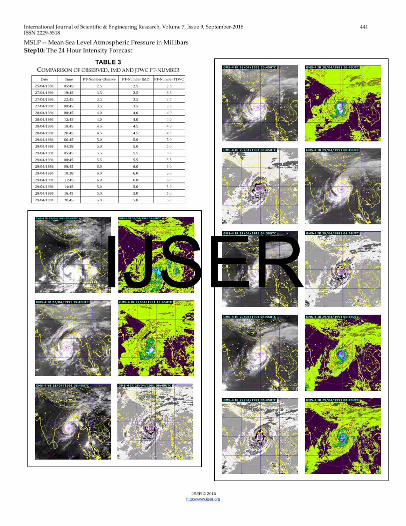
MSLP -- Mean Sea Level Atmospheric Pressure in Millibars Step10: The 24 Hour Intensity Forecast

TABLE 3 COMPARISON OF OBSERVED, IMD AND JTWC PT-NUMBER

Date Time PT-Number Observe PT-Number IMD PT-Number JTWC

25/04/1991 05:45 2.5 2.5 2.5

27/04/1991 19:45 3.5 3.5 3.5

27/04/1991 22:45 3.5 3.5 3.5

27/04/1991 00:45 3.5 3.5 3.5

28/04/1991 08:45 4.0 4.0 4.0

28/04/1991 12:45 4.0 4.0 4.0

28/04/1991 18:45 4.5 4.5 4.5

28/04/1991 20.45 4.5 4.5 4.5

29/04/1991 00.45 5.0 5.0 5.0

29/04/1991 04:38 5.0 5.0 5.0

29/04/1991 05:45 5.5 5.5 5.5

29/04/1991 08:45 5.5 5.5 5.5

29/04/1991 09:45 6.0 6.0 6.0

29/04/1991 10:38 6.0 6.0 6.0

29/04/1991 11:45 6.0 6.0 6.0

29/04/1991 14:45 5.0 5.0 5.0

29/04/1991 16:45 5.0 5.0 5.0

29/04/1991 20.45 5.0 5.0 5.0

IJSER




6 RESULTS AND DISCUSSION

The DVKT has been an important operational tool for estimat-ing tropical cyclone intensity and is the primary basis for the global tropical cyclone intensity climatology for the last 25 to 30 years. However, the DVKT remains the primary tool when aircraft reconnaissance is unavailable for this case. 25/04/91 (05:45utc) visible and enhanced picture shows shows the in-tensity of cyclone is more then CDO pattern so approximate PT number 2.5, which is same as JTWC and IMD PT number. 27 April 1991 this cyclone intensified in to a super cyclone with banding eye. All visible and enhanced picture shows its PT number is 5.5 to 6.0 which is also same as IMD and JTWC PT number.

7 CONCLUSION Correct classification of cyclone cloud patterns is important for the prediction of the cyclone evolution and weather predic-tion. Classification in turn depends on the accuracy of the pre-processing techniques applied to satellite images (both EIR and VIS). The DVKT has been an important operational tool for estimating tropical cyclone intensity. The satellite technol-ogy provides atmospheric weather observation over the earth. The tropical cyclone formation, tracking the position and mon-itoring of the intensity are now performed using digital inter-pretation techniques of the real time IR images. The cyclonical-ly and anticyclonically Curved bands are observed in the upstream environment of the disturbance. The straight diagonal line in the figure illu-strates the typical long-term growth rate observed in tropical cyclones. The rate is defined as one “T-number” per day. The T number is defined by the cloud features of a cyclone that are related to its intensity. Rapid and slow rates of growth are most often observed to occur at 1 ½ and ½ T-numbers per day, respectively. In 1991 cyclone, T number was change rapidly from 25-29 April.

8 REFERENCES Dvorak V. F. 1972 A technique for the analysis and forecasting of tropical cyclone intensities from satellite pictures. NOAA Tech. Memo. NESS 36, 15 pp.[Available from NOAA/NESDIS, 5200 Auth Rd; Washington, DC 20333] -1984; tropical cyclone intensity analysis using satellite data. NOAA Tech.Rep.11,45pp [Available from NOAA/NESDIS, 5200 Auth Rd; Washington, DC 20333] Dewan Abdur Quadir 2015 Advances of Space technology in Tropical Cyclone Research. Journal of Engineering Science 06(1&2), 2015,1-18 The Dvorak tropical cyclone intensity estimation technique by Christopher Velden etl. American Meteorological Society, Sep-tember 2006 BAMS-1195

Fig. 5. Observed PT Number form Infared image of Hima-wari Satellite


Index Terms IJSER · · 2016-10-02ern part of the Bay of Bengal, ... intensity estimates used for...

Documents

Transcript of Index Terms IJSER · · 2016-10-02ern part of the Bay of Bengal, ... intensity estimates used for...