Index

EVALUATION OF STRUCTURAL ANALYSIS METHODS USED FOR THE DESIGN OF TBM SEGMENTAL LININGS

A THESIS SUBMITTED TO THE GRADUATE SCHOOL OF NATURAL AND APPLIED SCIENCES

OF MIDDLE EAST TECHNICAL UNIVERSITY

BY

AHMET GÜRAY ÇİMENTEPE

IN PARTIAL FULFILMENT OF THE REQUIREMENTS FOR

THE DEGREE OF MASTER OF SCIENCE IN

CIVIL ENGINEERING

DECEMBER 2010

Approval of the thesis:


submitted by AHMET GÜRAY ÇİMENTEPE in partial fulfillment of the requirements for the degree of Master of Science in Civil Engineering Department, Middle East Technical University by, Prof. Dr. Canan Özgen Dean, Gradute School of Natural and Applied Sciences Prof. Dr. Güney Özcebe Head of Department, Civil Engineering Assist. Prof. Dr. Alp Caner Supervisor, Civil Engineering Dept., METU Examining Committee Members: Prof. Dr. Çetin Yılmaz Civil Engineering Dept., METU Assist. Prof. Dr. Alp Caner Civil Engineering Dept., METU Prof. Dr. Mehmet Utku Civil Engineering Dept., METU Assoc. Prof. Dr. Erdem Canbay Civil Engineering Dept., METU Harun Tulu Tunçay, M.Sc. Project Coordinator, YÜKSEL PROJE

Date:

http://web.ce.metu.edu.tr/index.php?id=25&sid=57�

iii

I hereby declare that all information in this document has been obtained and presented in accordance with academic rules and ethical conduct. I also declare that, as required by these rules and conduct, I have fully cited and referenced all material and results that are not original to this work.

Name, Last Name : Ahmet Güray Çimentepe

Signature :

iv

ABSTRACT


Çimentepe, Ahmet Güray

M.Sc., Department of Civil Engineering

Supervisor : Assist. Prof. Dr. Alp Caner

December 2010, 157 pages

Contrary to the linings of conventionally driven tunnels, the linings of tunnels

bored by tunnel boring machines (TBMs) consist of precast concrete

segments which are articulated or coupled at the longitudinal and

circumferential joints. There are several analytical and numerical structural

analysis methods proposed for the design of TBM segmental linings. In this

thesis study, different calculation methods including elastic equation method

and two dimensional (2D) and three dimensional (3D) beam – spring

methods are compared and discussed. This study shows that in addition to

the characteristics of concrete segments, the mechanical and geometrical

properties of longitudinal and circumferential joints have significant effects on

the structural behavior of segmental lining.

Keywords: TBM, Segmental Lining, Structural Analysis, Elastic Equation

Method, Beam – Spring Method

v

ÖZ

TBM İÇ KAPLAMA SEGMANLARININ TASARIMINDA KULLANILAN YAPISAL ANALİZ METOTLARININ DEĞERLENDİRİLMESİ

Çimentepe, Ahmet Güray

Yüksek Lisans, İnşaat Mühendisliği Bölümü

Tez Yöneticisi : Yrd. Doç. Dr. Alp Caner

Aralık 2010, 157 sayfa

Klasik metotlarla açılan tünellerin iç kaplamalarının aksine, tünel açma

makinalarıyla (TBM) inşa edilen tünellerin iç kaplamaları boyuna ve dairesel

yöndeki düğüm noktalarında kenetlenmiş ya da bağlanmış prekast

betonarme segmanlardan oluşmaktadır. TBM iç kaplama segmanlarının

tasarımı için önerilen birçok analitik ve nümerik yapısal analiz metodu

bulunmaktadır. Bu tez çalışmasında, elastik denklem metodu ile iki boyutlu

ve üç boyutlu çubuk – yay metotlarını içeren farklı hesaplama yöntemleri

incelenmiştir. Bu çalışma, betonarme segmanların niteliklerine ilaveten,

boyuna ve dairesel yöndeki düğüm noktalarının mekanik ve geometrik

özelliklerinin de segmanların yapısal davranışında önemli etkileri olduğunu

göstermiştir.

Anahtar Kelimeler: TBM, İç Kaplama Segmanı, Yapısal Analiz, Elastik

Denklem Metodu, Çubuk – Yay Modeli

vi

to my beloved wife, Buğçe

vii

ACKNOWLEDGEMENTS

I would like to express my deepest gratitude to my supervisor Dr. Alp Caner

for his endless supervision, trust, guidance and encouragement during and

beyond this work. Without his vision and support, I could never complete this

work.

I also would like to acknowledge the valuable comments and contributions of

my Supervising Committee Members.

Deepest thanks are dedicated to mom, dad and my brother. They were

always near me with their endless support.

And finally, words are not enough to express the role played by my wife,

Buğçe Doğan Çimentepe, to whom I owe most of beauty in my life. I proudly

dedicate this work to her so as to express my appreciation for her role.

viii

TABLE OF CONTENTS

ABSTRACT……………………………………………………….…………… iv

ÖZ………………………………………………………………….…….…….. v

ACKNOWLEDGEMENTS…………………………………….……………… vii

TABLE OF CONTENTS……………………………………..………………. viii

LIST OF TABLES…………………………………….……………………….. xi

LIST OF FIGURES………………………………….….…….………………. xiii

LIST OF ABBREVIATIONS……………………………………………......... xvii

CHAPTERS

1. INTRODUCTION……………………………….………………….…… 1

1.1. Foreword………………………………………..……………...….. 1

1.2. Scope and Objective of the Study…………..………….….….… 2

1.3. Thesis Overview……………………………………………...…… 3

2. OVERVIEW OF TUNNELING……………………… ……..………… 4

2.1. Brief History of Tunneling………………………………...……… 4

2.2. Classification of Tunnels…………………………………...……. 6

2.2.1. Type of Function…… …………………………………….. 6

2.2.2. Type of Construction Technique.………………….…….. 8

2.3. Essentials of Mechanized Shield Tunneling ………...………… 11

2.3.1. Structure and Dimensions of Tunnel Shields……….….. 12

2.3.2. Operations of Shield Machines……………………….….. 14

2.3.3. Classification of Tunnel Boring Machines (TBMs)…..…. 19

2.3.3.1. Rock Tunneling Machines……..………………… 21

2.3.3.2. Soft Ground Tunneling Machines..…….……….. 24

2.3.4. Selection of TBM……………………………………….…. 27

2.3.5. Conventional Tunneling versus Mechanized Shield

Tunneling……………………………...…………………... 28

ix

2.4. Segmental Tunnel Linings…………………... ………...….…….. 30

2.4.1. Geometry of Rings and Segments……………...……….. 31

2.4.2. Types of Rings and Segments…….………….………….. 35

2.4.3. Segmental Lining Materials..………………….………….. 38

2.4.4. Contact Surfaces…………...………………….………….. 39

2.4.4.1. Longitudinal (Segment) Joints .………..…...…… 40

2.4.4.2. Circumferential (Ring) Joints……….…….……… 42

2.4.5. Connectors..……………………….………………..….…... 45

2.4.6. Waterproofing System …………..………….……….….... 48

2.4.7. Ring Assembly………. …………..…………..……….…... 49

3. LITERATURE REVIEW..............................................……….…….. 52

3.1. Analysis Types……………………………………………..……… 52

3.1.1. Elastic Equation Method ………………………....………. 53

3.1.2. Schultze and Duddeck Method..……………..………….. 56

3.1.3. Muir Wood Method..……....…………………..……….….. 57

3.1.4. Beam – Spring Method..…...………………….………….. 58

3.1.5. Finite Element Method..…...………………….…….…….. 61

3.2. Theoretical Approaches on Beam – Spring Method.…...…..… 62

3.3. 2D and 3D Analysis of TBM Segmental Linings.……….……... 72

4. TBM SEGMENTAL LINING DESIGN..…………….………………… 75

4.1. Design Procedure………………..…………….…….……...……. 76

4.1.1. Design for the Ultimate Limit States..……….…….…….. 76

4.1.2. Design for the Serviceability Limit States..….………….. 77

4.1.3. Design Stages………………………...……….….……….. 77

4.2. Loading Conditions ……………..…………….….………...……. 79

4.2.1. Primary Loads……………………..………….…..…..…… 81

4.2.2. Secondary Loads……….…………………….…..…..…… 88

4.2.3. Special Loads……………..………………..……………… 90

4.3. Structural Calculation Procedure…..……….….…………….…. 92

4.3.1. Critical Sections…..………………..………….……...…… 92

x

4.3.2. Computation of Member Forces…………….…..…..…… 93

4.3.3. Safety of Section…………..………………..….……..…… 93

4.3.4. Limit State Design Method………..………….……...…… 94

4.3.5. Allowable Stress Design Method..………….…..…..…… 94

4.3.6. Safety of Joints..…………..……………….…………....… 95

5. METHODS OF ANALYSES……………….………..……….….……. 96

5.1. The Geometry of the Problem.……..………………….…...….. 97

5.2. Geotechnical and Material Parameters……….…..…………… 100

5.3. Analytical Analysis with Elastic Equation Method..…………… 101

5.4. Numerical Analyses………………………………………..…..… 102

5.4.1. 2D Structural Models….. ………………………....………. 106

5.4.2. 3D Structural Model…………..………………..………….. 110

5.5. Loading Conditions..…………………………………………….. 112

5.6. Flowchart of Calculation..……………………………………….. 114

6. RESULTS AND DISCUSSION………….…………………..…..……. 123

6.1. Evaluation of Analysis Methods…...………………………..….. 123

6.2. The Effect of Soil Stiffness on Beam – Spring Analysis…..…. 129

6.3. The Effect of Surcharge Load on Beam – Spring Analysis…. 131

6.4. The Effect of Mesh Coarseness on Beam – Spring Analysis.. 132

6.5. The Effect of Shear Spring Constant on Beam – Spring

Analysis………………………………………………………...… 134

6.6. The Effect of Segment Layout on Beam – Spring Analysis… 135

7. CONCLUSION……………………………………………………….… 137

REFERENCES…………………………………………….….…….…………. 139

APPENDICES

APPENDIX A. Working Sheets for the Analysis with Elastic

Equation Method…………………………..…….…... 145

APPENDIX B. Shear Spring Constants for 2D and 3D BSMs….... 150

xi

LIST OF TABLES

TABLES

Table 2.1. Comparison of major criteria for conventional tunneling and

TBM tunneling.……………………………………….……..……... 28

Table 2.2. Ranges for the dimensions of segmental linings……….…...…. 35

Table 3.1. Equations of member forces for Elastic Equation Method.….... 55

Table 4.1. Limit states for the design of segmental lining .…………….….. 76

Table 4.2. Classification of the loads for shield tunneling…….….…..……. 80

Table 5.1. Geotechnical parameters of the soil layers…………………….. 100

Table 5.2. General features of beam - spring models……………………... 105

Table 5.3. Summary of load conditions……………….…………………….. 113

Table 5.4. Combination of loads………………………………………….….. 114

Table 5.5. Soil stiffness for transition zones………………………………… 116

Table 5.6 Summary of load conditions for Case 3.…………….………….. 119

Table 5.7 Summary of analysis cases..…………………………………….. 122

Table 6.1. Analysis results obtained from elastic equation method and

2D beam – spring methods.……………………………………... 124

Table 6.2. Analysis results obtained from elastic equation method and

2D & 3D beam – spring methods.……………………….………. 127

Table 6.3. Analysis results obtained from 2D & 3D beam – spring

methods for the section passing though a soil transiton zone... 130


methods for the tunnel section subjected to surcharge load..... 131


methods for different mesh coarseness…………………….…... 133

Table 6.6. Analysis results obtained from 3D beam – spring methods

for three different shear spring constants……….……...………. 134

xii

Table 6.7. Analysis results obtained from 3D beam – spring methods

for four different segmental configurations………….….………. 136

xiii

LIST OF FIGURES

FIGURES

Figure 2.1. System groups of a tunnel boring machine…….………….... 15

Figure 2.2. Boring cycle of a TBM: a) Phase of advance, b) Installation

of segmental lining.…..…………………………………….….. 17

Figure 2.3. Shield tail with grouting of the ground-lining gap ………...… 19

Figure 2.4. Classification of tunnel boring machines (TBMs)……......…. 20

Figure 2.5. Rock tunneling machines: a) unshielded TBM, b) single

shielded TBM, c) double shielded TBM.……………….……. 23

Figure 2.6. Shield tunneling with a) mechanical support, b) compressed

air, c) slurry support, d) earth pressure balance..………….. 26

Figure 2.7. Ranges of diameters of different TBM types………..…..….. 27

Figure 2.8. Elements constituting a typical segmental ring….………..... 32

Figure 2.9. Segmental lining for a railway tunnel: a) ring position 1;

b) ring position 2; c) developed view………………………… 33

Figure 2.10. The cross-section of a typical TBM tunnel…..……………… 34

Figure 2.11. Conicity of segmental rings: a) type of rings; b) relationship

between conicity and minimum radius of curvature of the

tunnel...............................................…………………………. 36

Figure 2.12. Segment types…………………………….…………………… 37

Figure 2.13. Typical reinforcement cage for segmental linings………..... 39

Figure 2.14. Longitudinal joints with a) two flat surfaces, b) two convex

surfaces, c) convex / concave surfaces……………….…..… 41

Figure 2.15. Circumferential joint with flat surfaces………………...…….. 43

Figure 2.16. Circumferential joint with tongue-and-groove system…..…. 44

Figure 2.17. Circumferential joint with cam-and-pocket system…..….….. 45

Figure 2.18. Section of a typical housing for a single bolt……….…..…… 46

xiv

Figure 2.19. Section of a typical room for a single dowel…………...……. 47

Figure 2.20. Installation of segments and transmission of thrust forces

into the segmental linings……………………..…….………… 50

Figure 3.1. Load condition of Elastic Equation Method...…………..…… 54

Figure 3.2. Bedded ring model without crown bedding..………………... 57

Figure 3.3. Plain strain continuum model………………...………………. 58

Figure 3.4. Model of Beam – Spring Method…………...……….……….. 59

Figure 3.5. 3D Beam – Spring Model…..………………...………….……. 60

Figure 3.6. Finite element method for tunnel engineering………………. 62

Figure 3.7. Structural design models for TBM segmental linings.……... 63

Figure 3.8. a) Rotational spring model, b) Stress distribution at the

segment joint...………………………..…...…………….…..… 68

Figure 3.9. Stress and deformation in mortised portions…………....….. 69

Figure 3.10. Forces acting on the ring joints and joint displacements….. 71

Figure 4.1. Flowchart of shield tunnel lining design.…………….………. 79

Figure 4.2. Notations of bending moment, axial force and shear force.. 81

Figure 4.3. Section of tunnel and surrounding ground…..…………….... 82

Figure 4.4. Calculation of loosening ground load.……..……….……….. 84

Figure 4.5. Ground pressures acting on lining.....………………….……. 86

Figure 4.6. Hydrostatic pressure………………..…………………..…..… 86

Figure 4.7. Interaction diagram…………………..…………………..……. 94

Figure 5.1. Tunnel cross-section…………………...………………..……. 98

Figure 5.2. Geometry of the problem.………………………….……..…... 99

Figure 5.3. Typical 2D beam – spring model composed of 50

members……………………………………………….……….. 102

Figure 5.4. Typical 3D beam – spring model composed of 50

members…………………………………………….………….. 103

Figure 5.5. Ground spring constants……………………...…….…...……. 104

Figure 5.6. Configuration of segment joints in 2D models.……..….…… 107

xv

Figure 5.7. The relationship between the M/N ratio and joint rotational

stiffness kθ (for reference purpose only)………...………….. 108

Figure 5.8. The iteration process for the computation of joint rotational

stiffness……………………….…………………..………….… 110

Figure 5.9. Configuration of segment joints in 3D models..………….... 111

Figure 5.10. Shear spring constant………………………..….………….… 112

Figure 5.11. Soil profile of the tunnel route…………….….….…………… 115

Figure 5.12. Theoretical and computational models of the rotational

spring constant………………………………….…..…………. 117

Figure 5.13 Longitudinal profile of the tunnel under surcharge…..…..… 118

Figure 5.14. Segment configurations for 4 different layouts……...……… 121

Figure A.1. Input sheet for the analysis with Elastic Equation Method... 146

Figure A.2. Load conditions sheet 1 for the analysis with Elastic

Equation Method………………………………………………. 147

Figure A.3. Load conditions sheet 2 for the analysis with Elastic

Equation Method………………………………………...…….. 148

Figure A.4. Member forces sheet for the analysis with Elastic

Equation Method………………………………………………. 149

Figure B.1. Rotational Stiffness vs. M/N diagram for 2D BSM in

Case 1…………………………………………………………... 150

Figure B.2. Rotational Stiffness vs. M/N diagram for 3D BSM in

Case 1…………………………………………………………... 150

Figure B.3. Rotational Stiffness vs. M/N diagram for 2D BSM

consisting of 50 beam elements in Case 4………………….. 151


consisting of 150 beam elements in Case 4...…………..….. 151


consisting of 250 beam elements in Case 4...…….….…….. 152


consisting of 50 beam elements in Case 4...……….……..... 152

xvi


consisting of 150 beam elements in Case 4...……….….….. 153


consisting of 250 beam elements in Case 4...………..…….. 153


(Ks=15000 kN/m) in Case 5...……………………………..….. 154


(Ks=20000 kN/m) in Case 5...……………………..………….. 154


(Ks=25000 kN/m) in Case 5...……………………..………….. 155


(Layout 1) in Case 6..……………………………….…………. 155


(Layout 2) in Case 6...……………………………...………….. 156


(Layout 3) in Case 6..........................................…………….. 156


(Layout 4) in Case 6..........................................…………….. 157

xvii

LIST OF ABBREVIATIONS

ACI American Concrete Institute

AFTES French Tunnelling and Underground Engineering Association

BSM Beam – Spring Model

DAUB German Committee for Underground Construction

DIN Deutsche Industrie-Norm

FEM Finite Element Method

ITA International Tunneling Association

JIS Japanese Industrial Standard

JSCE Japan Society of Civil Engineers

NATM New Austrian Tunneling Method

SIG Italian Tunnelling Association

SLS Serviceability Limit State

SNIP Standard and Russian Construction Norms and Regulations

TBM Tunnel Boring Machine

ULS Ultimate Limit State

2D Two Dimensional

3D Three Dimensional

1

CHAPTER 1

INTRODUCTION

1.1. Foreword Rapid world-wide urbanization have recently accelerated subterranean and

tunnel construction [1]. Tunnels provide transportation routes for rapid transit,

railroad and vehicular traffic, conveying both fresh water and waste, and

transferring water for hydroelectric power generation. Moreover, they are

utilized as conduits, canals, passageways for pedestrians, and used for

mining, industrial cooling, storage, and military works [2]. As the demands on

passenger and goods transportation increase with social and industrial

development, the necessity and importance of tunnels have been extensively

discovered.

Tunnels are built in several different underground environments, including

soil, rock, mixed soil and rock, with extended variations in the groundwater

conditions, in-situ states of stress, and geological structures. Alternative

construction techniques, including hand excavation, drill-and-blast methods,

cut and cover, and various mechanical tunneling equipments, are used to

construct tunnels [2]. Especially in urban regions, the mechanized tunneling

has consistently increased due to the ascending number of tunnels

constructed for subways, railway underpasses, and urban highways.

However, tunneling in urban areas generally brings to minds high-level risks,

which may result in potential damage to structures and people [3]. In such a

complex and risky type of structure; not only the construction phase, but also

the design stage is of vital importance.

2

Enhanced demands and potential risks have led to development in the art

and technique of tunneling especially in design and analysis methods.

Accordingly, extensive improvements in the scientific background of

tunneling, mainly by the scientific advances made in tunnel mechanics, have

been developed [1]. Several structural design models including various

analytical closed form solutions and bedded beam-spring approaches have

been improved. Closed form solutions, restricted to a number of

simplifications, are arguably cheaper and quicker to use. These simplified

two-dimensional models have been used mostly in Austria and Germany. On

the other hand, bedded Beam - Spring Models (BSMs) which represent the

lining as a string of interconnected pin-ended structural beams, and the

ground as a series of radial springs are the most common structural analysis

tools used in shield tunneling design. Two-dimensional (2D) and three-

dimensional (3D) applications of BSMs have been used worldwide, especially

in Germany, Belgium, France, Japan, and United States [4]. Detailed

researches on these structural models which predict the behavior of tunnel

during and after the excavation are necessary for the proper design of

segmental tunnel linings.

1.2. Scope and Objective of the Study In a tunnel design, the same cross-section is used even the loads or soil

conditions change along the route. In this study, the most commonly applied

structural analysis methods used in the design of shield tunneling are

investigated. Shield tunneling is a typical structural system selected for

railroad tunnels. The scope of this thesis covers the evaluation of different

structural analysis methods used for the design of segmental tunnel linings.

“Elastic Equation Method” proposed by Japanese Standard for Shield

Tunneling has been selected as an analytical approach. Furthermore, several

BSM approaches have been selected as numerical methods. Then, both

analytical and numerical methods have been examined for different mesh

coarseness, loading conditions, soil stiffness, ring joint stiffness, and

3

segment configurations for the analysis of shield tunneling especially for

tunnels excavated and shielded by Tunnel Boring Machines (TBMs).

The aim of this study is to compare and evaluate commonly used structural

analysis methods for the design of segmental tunnel linings under certain

situations. Strength and weaknesses of the methods will also be identified.

1.3. Thesis Overview This thesis study has seven chapters. Chapter 1 (Introduction) generally

presents the main subject, the objective and scope of the study. In Chapter 2

(Overview of Tunneling), brief history of tunneling, types and geometry of

tunnels, and general knowledge on mechanized shield tunneling and TBM

segmental linings are introduced. Chapter 3 (Literature Review) describes

the theoretical background of structural analysis methods used in the design

of TBM segmental linings and gives a summary of previous studies. Chapter

4 (TBM Segmental Lining Design) briefly indicates the design procedure,

loading conditions, and structural calculation procedure used in the design of

segmental tunnel linings. In Chapter 5 (Methods of Analyses), studies having

done throughout this project are detailed. In Chapter 6 (Results and

Discussion), comparison and evaluation of analysis results are made.

Chapter 7 (Conclusion) summarizes the thesis study and gives the

recommendations for further studies.

4

CHAPTER 2

OVERVIEW OF TUNNELING

In this chapter, a compendious overview of tunneling history, tunnel types

(especially mechanized tunneling), tunnel geometry, principles of

mechanized shield tunneling, tunnel boring machines, and segmental tunnel

linings is provided.

2.1. Brief History of Tunneling The history of tunneling extends up to the prehistoric era. Throughout the

ages, mankind used tunnels for many purposes such as defense, assault,

production, storage, communication, and transportation. The areas of usage

for first tunnels were communication, mining operations and military

purposes.

The oldest tunnel was constructed for the aim of communication nearly 4000

years ago. It was built to underpass the bed of the River Euphrates and to

link the royal palace to the Temple of Jove in ancient Babylon. This tunnel

has a length of 1 km with cross-section dimensions of 3.6 m by 4.5 m. Its

walls consist of brickwork laid into bituminous mortar and a vaulted arch

covers above the section. These details and scope of the work, which require

broad experience and skill, show that this tunnel was not the first tunnel

constructed by the Babylonians. Salt mine in Hallstatt and flint mines in

France and Portugal are the earliest examples of prehistoric tunnels used for

mining operations [5].

5

Tunnels for water conveyance were mostly built by Romans. Advanced

surveying techniques to drive tunnels from both portals towards the middle of

tunnel were firstly utilized by Greeks about 500 B.C. This was a great

development which reduced excavation time and labor need. Also, tunnels

built by Romans can be distinguished with their long service life due to the

Roman philosophy that a civil engineering work had to last forever [6].

With the utilization of gunpowder in tunneling during the Renaissance era,

conventional methods such as shovels, picks, and water have been replaced

by blasting. Ventilation systems have also been improved in order to clean

the smoke immediately after blasting [6].

Marc Isambard Brunel, inventor of shield tunneling, tried his system in great

Thames Tunnel. Brunel’s first shield was rectangular and tunnel was lined

with brickwork. After great difficulties involving five serious floods, the double

track tunnel was completed in 1842. Then, James Henry Greathead

improved first cylindrical shield and employed this shield in London in 1869

for the construction of Tower Tunnel underneath Thames River. He also used

cast iron lining segments for the first time [1, 7].

Inventions by Brunel and Greathead became the model for further

developments in shield and mechanized tunneling. In the last century, air-

compressed, slurry, and earth-pressure balance shields have been

developed and these advances enabled the daily peak advance of 25 cm

obtained by Brunel to be increased to 25-30 m [1].

A very quick overview in the history of tunneling has been discussed by

emphasizing the milestones in tunnel construction. Advances in tunneling are

still proceeding progressively by introducing and perfecting modern free face

and shield methods that permit the large scale use of high capacity

mechanical equipment [1].

6

2.2. Classification of Tunnels Tunnels can be classified according to their functions, the method of

construction, the geological situation, and the hosting medium, etc.

Especially, functionality and the excavation method are the common criteria

for the categorization of tunnels. General information about the certain types

of tunnels in terms of their functionality and construction technique is given in

the proceeding sections.

2.2.1. Type of Function Direct transportation of passengers and goods through the certain obstacles

is the main purpose of tunnels. Obstacles to be underpassed can be a

mountain, river, industrial, or dense urban areas, etc. The purpose of

overcoming these obstacles may be to carry road, railway, or pedestrian, to

convey water, gas, sewage, or to provide indoor transportation for industrial

plants [1].

The classification according to these purposes can be summarized as

follows:

a) Highway Tunnels: Highway tunnels are only a part of larger highway

systems. Providing a crossing under an obstacle, which is the main function

of these tunnels, has a great importance in linking up remote areas as under

an estuary or through a mountain range. Highway tunnels are designed in

accordance with their traffic capacity, lane widths and clearances, gradients

and traffic composition. Moreover, their special construction characteristics

include geometrical configuration, road construction, lighting, ventilation,

traffic control, fire precautions, and general facilities for cleaning and

maintenance [8].

Depending on the shape, i.e. rectangular, circular or horseshoe; cut-and-

cover, blasting, New Austrian Tunneling Method (NATM), or mechanized

7

shield tunneling with TBMs can be used as an excavation method for

highway tunnels [8]. Also, highway tunnels more than 3 km long require

vertical shafts for ventilation, otherwise just horizontal ventilation is

permissible.

b) Railway Tunnels: Tunnels, essential features of railway systems, are

mostly used to provide a track with a limited gradient. An acceptable gradient

governs the longitudinal profile of all railway tunnels. Generally, a gradient

less than 1% is preferred but steeper gradients may have to be adopted in

many cases. Another principal geometrical factor is curvature, which is

governed by speed of trains [5].

Mountain ranges, hills, and subaqueous crossings are the typical situations

for main line railways. Every kind of ground such as shattered rock,

squeezing rock, silt, clay, etc. is liable to be encountered. In modern railway

tunnels, NATM with sprayed concrete, steel arch ribs, and in situ concrete

applications is the most usual excavation method. Apart from NATM, shield

tunneling with segmental concrete or even cast iron linings is also preferred

depending on the project characteristics [5].

c) Metro Tunnels: Metro tunnels are special types of railway systems

adapted to cities and their immediate environs. The most distinctive feature

of a metro system is the rapid transportation of numerous people on an

exclusive right of way without any interruption by other types of traffic.

Differently from railway tunnels, metro tunnels are used for shorter and more

frequent journeys, and they may have a steeper gradient due to the fact that

no heavy good trains are used in metro lines [8].

Metro systems are preferred to meet the needs of cities where centers are

closely built up that surface railways or elevated railways are quite

impracticable. Cut-and-cover under existing streets and boring with TBM

8

under streets and buildings are widely used excavation methods of metro

tunnels [8]. These types of tunnels require ventilation systems.

d) Pedestrian Tunnels: Since the pedestrians can descend and ascend

steps or quite steep gradients, and turn sharp corners, pedestrian subways

are the least demanding and the most primitive type of tunnels. Therefore,

the absolute limitations on this type of underground structures are very few.

On the other hand, pedestrian subways should be as shallow as possible,

because long descends and ascends may discourage the users anyhow. In

the construction of shallow subways, cut-and-cover method is preferred.

However, boring is better to perform excavation for connecting passages in

metro stations at deeper level [5].

e) Conveyance Tunnels: Conveyance tunnels are built to convey water or

sewage in many fields for various purposes. Fresh water supplies for cities,

canals, irrigation, discharge tunnels for hydroelectric power, and dam bypass

tunnels can be certain examples for conveyance tunnels. Smoothness and

watertightness are the basic characteristics required for this type of tunnels.

Smoothness depends on the velocity of water and the length of the tunnel.

Besides, watertightness is dependent on internal and external pressure [5].

Segmental linings meet the requirements for watertightness and smoothness

better than other tunneling methods. Hence, shield tunneling is generally

performed for the excavation of large-scale conveyance tunnels. If boring

with TBM is not feasible, conventional methods are also applicable.

2.2.2. Type of Construction Technique

In this section, three common construction methods used in tunneling are

mentioned briefly. These methods taken into consideration are cut-and-

cover, New Austrian Tunneling Method (NATM), and Mechanized Shield

Tunneling. Apart from these methods, there are some other techniques

9

including drilling and blasting, earth boring, pipe jacking, immersed tube, and

floating tunnels used for special cases.

a) Cut-and-Cover: Cut-and-cover is an alternative tunnel construction

technique where a trench of the required depth and width can be excavated

from the surface. This method can simply be summarized that a trench is

excavated, the tunnel structure is constructed, then the trench is backfilled,

and finally the surface is restored. Due to the support of soft ground and

maintenance of surface and underground facilities, most projects become

much more complex.

Cut-and-cover is a practical and an economical technique for tunnel

constructions in shallow depth and in loose ground. This method offers more

feasible solutions than tunneling up to depths of 10 m in open trenches.

However, incidental costs may change the situation completely. These costs

including provision of alternative facilities for traffic using the surface,

safeguards against subsidence, protection or diversion of services and

drainage systems, social costs of disruption, and loss of amenity may usually

be unavoidable in urban areas. Therefore, the choice between cut-and-cover

and boring should be made by performing a detailed cost – benefit analysis

[8].

Cut-and-cover tunnels are commonly implemented in subaqueous tunnels to

form a transition between an open cut approach and the main tunnel, at the

portals of mountain tunnels, in urban conditions where the route must be

covered in, and the surface restored.

b) New Austrian Tunneling Method (NATM): NATM, introduced by

Rabcewicz (1969), is an observational method and requires application of a

thin layer of shotcrete with or without rockbolts, wire mesh fabric, and lattice

girder; and monitoring and observing the convergence of the opening. The

10

shotcrete thickness is optimized with respect to the admissible deformations.

Consecutive shotcrete applications are necessary until the convergence has

stopped or it is within the acceptable range [6].

In NATM construction technique, tunnel is sequentially excavated and

supported. The primary support is provided by the shotcrete in combination

with or without steel mesh, lattice girders, and rockbolts. Cast in-situ concrete

lining is installed as secondary lining which is designed separately [9].

Especially in soft ground or weak rock, partial face excavation is performed.

By this way, several headings with small cross-sections are chosen to

minimize ground loading on it. This enables to support headings succesively.

When the top heading has advenced far enough, bench excavation begins,

with ramps left in place for access to the top of the heading [10].

NATM method is commonly performed in large railway, highway, and water

conveyance tunnels. Its primary advantage is the economy because of

matching the amount of support installed to the requirements of the ground

loading rather than having to install worst case support throughout the tunnel

[10].

c) Shield Tunneling: Particularly, tunneling with a shield is well adapted for

softer soils and weaker rocks which need continuous radial support. The

shield is a rigid steel cylindrical tube providing facilities at its front for the

excavation of ground material and at its rear for the erection of the

prefabricated lining. It has to be designed to be able to take all ground and

working loads with relatively small deformations. The front of shield is

equipped with cutters that perform excavation. Jacks installed in the shield

are used to push the shield away from the installed lining into the ground.

The tunnel advance ranges from 0.8 m to 2.0 m depending on the length of

segments. Then, segmental lining is placed and the gap between the lining

11

and ground is filled with grout. This cycle continues up to end of tunnel

construction [1, 9].

Shield-driven tunnels may have single or double linings. When the functions

of double layer in terms of resistance to external pressures, watertightness or

aesthetic appearance can not be provided by single layer, double layers are

performed. The earliest lining type for shield tunneling was made of bricks.

However, cast-iron segments, structural steel segments, and reinforced

concrete segmental linings have recently been in use. These modern lining

segments have an ability to resist larger pressures and to provide better

watertightness [1].

Tunnels having different sizes with diameters ranging from 0.10 m up to 19 m

can be excavated by different types of mechanized shields and with different

processes. Broader knowledge on working principle, excavation, support and

installation procedures, components, and classification of shield tunneling will

be provided in the proceeding chapter.

2.3. Essentials of Mechanized Shield Tunneling According to the French Association of Tunnels and Underground Space

(AFTES), “the mechanized tunneling techniques” (as opposed to the so-

called “conventional” techniques) are all the tunneling techniques in which

excavation is performed mechanically by means of teeth, picks, or discs.

Within the mechanized tunneling techniques, all categories of tunneling

machines range from the simplest one (backhoe digger) to the most

complicated one (shield TBM) [11]. However, this thesis study covers only

tunneling operations with TBMs that allow full-face excavation.

The tunnel shield is a moving metal casing, which is driven in advance of the

permanent lining, to support the ground surrounding the tunnel-bore and to

afford protection for construction of the permanent lining without any

12

temporary support. Actually, the shield is a rigid steel cylinder open at both

ends, providing facilities at its front for the excavation of the ground material

and at its rear for the erection of the prefabricated lining. Thus, the shield is

always forced ahead by steps keeping pace with the progress of excavation

and erection work to the extent that the excavated hole should be well

supported until the permanent lining is constructed.

A full cycle of shield tunneling involves the following steps:

• excavation and temporary support of the front face at a suitable depth

• advancing the shield, taking support on the previously erected lining

• placing another course or ring of the permanent lining.

This cycle is repeated up to the completion of tunnel construction [1].

2.3.1. Structure and Dimensions of Tunnel Shields The skin is the principle element of the shield. It is constructed of steel plates

and bent to the shape of the tunnel section. Cylindrical skin is slightly larger

than the outer diameter of tunnel for the proper placing of segmental linings.

The skin may be divided into three main parts differing in their inner rigidity

and arrangement in accordance with their purpose.

1. The front part of the skin, where excavation is performed is heavily

reinforced, generally with steel castings to form the cutting edge, its inner

rigidity being increased by stiffening rings. Its main aim is to perform the

smoothest possible advance and steerability of the shield skin by cutting the

face, and to provide pressure distribution as uniform as possible induced

ahead.

Its secondary duty is to give an adequate shelter to the workmen engaged in

the excavation, through affording a certain support for the front face.

13

2. The trunk (or intermediate) part is formed for the housing of pushing

machinery (hydraulic jacks, high-pressure pump installations, etc.).

3. The tail part of the shield is designed for the erection of segmental linings.

In addition to these parts, some important complementary elements are

integrated in the interior of the shield mostly in combination with its stiffening

elements, such as working platforms, or front-support jacks [1].

After the determination of structural elements, shape and dimensions of the

main shield should be emphasized. Typically, a circular shape is selected for

shields, because this shape shows the best resistance to outside pressures.

Moreover, this is the most suitable shape that allows forming bolted joints

between the consecutive rings easily and exactly. If shields of oval or

rectangular shape are used, a greater pushing force will be required for the

advance as compared to circular tunnels. In addition to advantages

mentioned above, a bigger arching action will take place above circular

shields leading to a decrease in rock pressure and in frictional resistance.

The clearance requirements of tunnel definitely determine the diameter of the

shield. In this sense, all operations (excavation, mucking, transport, erection)

must be performed and all mechanical equipment (jacks, pressure pumps,

platforms and conduits, erectors, loading machines, etc.) must be installed

within the limited inner space of the shield. A reasonable economical

selection that meets the requirements mentioned above must be made.

The choice of a suitable shield length is a major problem in the design of

shield machines. The length is mainly determined by the dimensions of the

jacks and the lining segments. The operating conditions of the shield are

mostly affected by the relative length, i.e. by the shield diameter compared

with shield length (L/D). This ratio affects the steerability, mobility, and the

14

steadiness of its direction. The shorter the shield, the more difficult it is to

keep it in the correct line and the easier it is to change of its direction on

curves. On the other hand, the longer the relative length of the shield, the

easier it is to keep it in its original direction, but the more difficult to bring it

back from an accidental incorrect direction. The ratio of relative length ranges

between 0.4 and 1.4. However, according to the present considerations, this

ratio should not exceed 0.70 – 0.75 [1].

According to Richardson and Mayo [12], the approximate steel weight of a

tunnel shield can be obtained by the following formula:

( )1015 −⋅= DW (2.1)

where, W : the weight of shield in tons,

D : the external diameter in feet.

2.3.2. Operation of Shield Machines The main components of a TBM are: 1) cutterhead, 2) cutterhead carrier with

the cutterhead drive motors, 3) the machine frame, and 4) clamping and

driving equipments. The necessary control and ancillary functions are

connected to this basic construction on one or more trailers.

The operation systems of shield machines can be divided into four groups;

• Boring (Excavation) System

• Thrust and Clamping System

• Muck Removal System

• Support System

These system groups and their main parts are given in Figure 2.1.

15

Figure 2.1. System groups of a tunnel boring machine [13]

a) Boring (Excavation) System: The boring system which determines the

performance of a TBM is the most critical part. It consists of various

excavation tools which are mounted on a cutterhead. The range of

application of these excavation machines depends on the surrounding

ground [14].

For easily to moderately removable soils, cutting wheels equipped with drag

picks or steel pins are used. A small cutting wheel in the center of the main

cutting wheel is frequently arranged in cohesive soils. By this way, centric

cutter rotates independently from the main cutting wheel and avoids

adhesion by means of an increased circumferential speed.

In hardly excavatable soils and easily excavatable rocks, cutterheads

equipped with cutter discs and drag picks are used. On the other hand, in

16

hardly excavatable rock, cutterheads solely equipped with discs are used

[15].

The discs are arranged in an order so that they contact the entire cutting face

in concentric tracks when the cutterhead turns. The separation of the cutting

tracks and the discs are selected according to the ground type and the ease

of cutting. This selection also designates the size of the broken pieces of

ground.

The rotating cutterhead pushes the discs with high pressure against the face.

Therefore, the discs make a slicing movement across the face. As the

pressure at the cutting edge of the disc cutters exceeds the compressive

strength of the rock, it locally grinds the rock. As a result, the cutting edge of

the disc pushes rolling into the rock, until the advance force and the hardness

of the rock come to equilibrium. Through this net penetration, the cutter disc

creates a locally high stress, which causes long flat pieces of rock breaking

off [13].

b) Thrust and Clamping System: The thrust and clamping system is an

element which affects the performance of a TBM. It is responsible for the

advance and the boring progress. The cutterhead with its drive unit is thrust

forward with the required pressure by hydraulic cylinders which are illustrated

in Figure 2.2a. The maximum stroke is governed by the length of the piston

of the thrust cylinder. Today, TBMs achieve a stroke value of up to 2.0 m.

After a bore stroke has been bored, the boring process is interrupted so that

the machine can be moved with the help of the clamping system. The shield

TBM is stabilized during this process by the clamping at the back and the

shield surfaces around the cutterhead.

17

Figure 2.2. Boring cycle of a TBM: a) Phase of advance, b) Installation of

segmental lining [14]

The thrust system limits the possible thrust and must resist the moments

caused by the rotation of the cutterhead. The limits on the applied clamping

forces are determined by the condition of segmental lining, because TBMs

except for double shielded ones can not be braced radially against the tunnel

walls but they are braced axially against the lining. For that reason, the

segmental lining, not the rock strength, is decisive for shield TBMs [13].

c) Muck Removal System: One of the major problems of efficient tunnel

driving is the effective muck haulage. It is performed in two steps in case of

shield tunneling. The first step is the removal of soil from the shield body and

the second is its conveyance to the ventilation or working shaft. Firstly, the

18

muck is collected at the face by cutter buckets and delivered to the conveyor

down transfer chutes. Then, the muck is transported from the completed

tunnel section to the access shafts or to the tunnel portals [1, 13].

A powerful system should be selected in order to ensure the carrying away of

the muck throughout the entire tunnel. Moreover, the system equipments

must make the smallest possible demand on space, since the removal

system should not interfere with the supply of the TBM and necessary

support measures. For this purpose, a rail system or a conveyor system is

suitable according to local conditions. Furthermore, large dump trucks can

alternatively be used for certain conditions [13].

d) Support System: In shield tunneling, the shield provides the temporary

support of the rock around the shield. The shield casing begins directly

behind the circumferential discs and also encloses the area where the

support elements are installed. Reinforced concrete segments, which are

mostly used for the support, are installed singly by the erector and form an

immediate support. A shield TBM can be equipped with compressed air,

hydraulic or earth pressure support and then it can be used under the water

table [13].

Segmental lining elements are erected with a hydraulically-operated erector

arm which can be mounted either directly on the axis of the shield tail or on a

travelling working platform following closely behind the shield [1]. This stage

is illustrated in Figure 2.2b.

Figure 2.2a shows that the shield tail, the rearmost part of the shield,

overlaps the last segment and keeps the ground from deforming or falling

into the excavated tunnel.

19

As shown in Figure 2.3, any possible loosening of the ground is prevented by

grouting the annular gap. Also, a connection between ground and lining is

provided. In order not to hinder the advance or interrupt it for a longer period,

the rear carriage must contain all the equipment necessary for a rapid

installation.

Moreover, a sealing is installed between shield tail and segmental ring in

order to prevent the continuous grouting to flow into the shield. During tunnel

advance, this sealing is sliding over the linings [4, 13].

Figure 2.3. Shield tail with grouting of the ground-lining gap [4]

2.3.3. Classification of Tunneling Boring Machines In the scope of this thesis, it is necessary to have a general overview of

TBMs. In this section, the most widely-used types are emphasized.

The problem with the classification of tunneling machines is that there is no

unitary definition and classification for tunneling machines accepted globally.

However, the term Tunnel Boring Machine (TBM) is now universally adopted

for all the machines that have a full-face cutting wheel for excavating a tunnel

[3].

20

French Tunneling and Underground Engineering Association (AFTES),

German Committee for Underground Construction (DAUB), Japan Society of

Civil Engineers (JSCE), and Italian Tunneling Association (SIG) are all

leading national tunneling associations and have their own classification

system for tunneling machines based on different criteria. However, the

classificaiton to be considered in this study is based on what have been

developed by International Tunneling Association (ITA) Working Group 14

“Mechanized Excavation”. TBMs are subdivided according to both the

support typology that the machine is able to supply and the type of ground

that it is able to operate in.

Like in the ITA and AFTES classifications, the term TBM also refers to all

tunneling machines allowing full-face excavation in this study.

Figure 2.4 illustrates the classification scheme adopted in this study and the

TBM types given in this classification are explained in terms of general

characteristics, application field, and working principle in the following

chapter.

Figure 2.4. Classification of tunnel boring machines (TBMs)

21

2.3.3.1. Rock Tunneling Machines

Unshielded TBMs are typical rock machines used when rocks with good to

very good conditions are excavated and they need to be associated with

primary support system as for excavation using conventional method (rock

bolts, shotcrete, steel arches, etc.). As shown in Figure 2.5a, a cutterhead is

pushed against the excavation face by a series of thrust jacks, but the jacking

forces are not transferred to the tunnel lining. “Grippers” which apply a force

at the tunnel walls to clamp the machine to the rock mass are used. The

cutters penetrate into the rock, creating intense tensile and shear stresses

and then crushing it locally. The muck is collected by special buckets in the

cutterhead and removed by primary mucking system. Although the machine

is not equipped with a circular shield, a small safety crown-shield is provided

at the back of the cutterhead.

The working cycle of unshielded TBMs includes: 1) gripping to stabilize the

machine; 2) excavating for a length equivalent to the effective stroke of the

thrust jacks; 3) regripping; 4) new excavation [16].

Single Shielded TBMs are typical ground or weak rock machines used

when it is necessary to support the tunnel very soon with precast lining. The

excavation procedure is the same with unshielded machines. As seen in

Figure 2.5b, the support to the advancing thrust is provided by the precast

segments constituting the tunnel lining. This machine is equipped with a full

round protective shield immediately behind the cutterhead.

The working cycle of single shielded TBMs includes: 1) excavating for a

length equivalent to the effective stroke of the thrust jacks; 2) assembling of

segmental linings and retraction of the jacks; 3) new excavation [3, 16].

Double Shielded TBMs are very flexible and useful machines especially in

mixed rock conditions. They are similar to single shielded TBMs, but offer the

22

possibility of a continuous work cycle owing to double thrust system. This

machine is more versatile than the single shield, since it can move forward

even without installing the tunnel lining or install segmental linings during

excavation depending on the ground stability conditions [3, 16].

Figure 2.5c demonstrates the double thrust system which consists of a series

of longitudinal jacks and a series of grippers positioned inside the front part of

the shield. Longitudinal jacks use the tunnel walls to brace against the thrust

jacks. Also, advance without installing segmental linings is performed by

these longitudinal jacks.

23

Figure 2.5. Rock tunneling machines: a) Unshielded TBM, b) Single shielded

TBM, c) Double shielded TBM [14]

24

2.3.3.2. Soft Ground Tunneling Machines

Open Shield is a tunneling machine in which face excavation is

accomplished using a partial section cutterhead. There are hand shields and

partly mechanized shields at the base of the excavating head. Excavation is

performed by using a roadheader or using a bucket attached to shield, and

using an automatic unloading and mucking system.

Open shields are used for rock masses whose characteristics vary from poor

to very bad, cohesive or self-supporting ground in general [16].

Mechanically Supported Close Shield is a TBM in which the cutterhead

plays the dual role of acting as the cutterhead and the supporting the face.

As shown in Figure 2.6a, steel plates may be installed in between the free

spaces of the cutting arms, to slide along the cutting face while rotating the

boring machine. The debris is extracted through adjustable openings or

buckets and conveyed to the primary mucking system.

This method is suitable for soft rocks, cohesive or partially cohesive ground,

and self supporting ground above the ground water table [4, 16].

Compressed Air Closed Shield is used to support the face by compressed

air at a suitable level to balance the hydrostatic pressure of the ground. A

typical working scheme is given in Figure 2.6b. The debris is extracted from

the pressurized excavation chamber using a ball-valve-type rotary hopper

and then conveyed to the primary mucking system.

This method is applied to grounds with medium-low permeability under the

ground water table to avoid water influx [4, 16].

Slurry Shields stabilize the tunnel face by applying pressurized bentonite

slurry as illustrated in Figure 2.6c. The soil is mixed into the slurry during the

25

operation and at the end, the soil is removed from the slurry in a separation

plant. The separation plant is generally located on the surface. A chamber

with air pressure is connected to the slurry in order to control the slurry

pressure.

This type of TBM is preferred in soft soils with limited self-supporting

capacity. In other words, slurry shields are commonly suitable for excavation

in ground composed of sand and gravels with silts under the ground water

table [3, 16].

Earth Pressure Balance Shields are most commonly used TBMs in soft

grounds. As illustrated in Figure 2.6d, face support is provided by the

excavated earth which is kept under pressure inside the excavation chamber

by the thrust jacks. Excavation debris is removed from the excavation

chamber by a screw conveyor which enables the pressure control by

variation of its rotation speed.

This method is mainly used in soft ground with the presence of ground water

and with limited or no self-supporting capacity. In other words, typical

application fields are silts or clays with sand. Furthermore, excavation in rock

is possible with the use of disc cutters [3, 16].

Apart from these, there are special types of tunnel boring machines including

hydroshields, mixshields, double tube shields, flexible section shields, etc.

used in particular cases.

26

Figure 2.6. Shield tunneling with a) mechanical support, b) compressed air,

c) slurry support, d) earth pressure balance [4]

27

2.3.4. Selection of TBM One of the most important strategic decisions in mechanized shield tunneling

is the selection of the most appropriate TBM type. The selected machine

should be able to deal the best with the ground conditions expected [17].

The type and configuration of TBM are decided depending on the size of the

tunnel and the geological conditions of the rock. Geological factors affecting

the TBM selection are: grain size distribution, type of predominant mineral

(quartz contents), soil strength, overburden, heterogeneity, and piezometric

pressure [18].

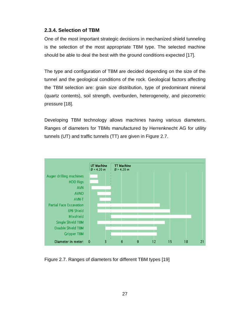
Developing TBM technology allows machines having various diameters.

Ranges of diameters for TBMs manufactured by Herrenknecht AG for utility

tunnels (UT) and traffic tunnels (TT) are given in Figure 2.7.

Figure 2.7. Ranges of diameters for different TBM types [19]

28

2.3.5. Conventional Tunneling versus TBM Tunneling Tunnel projects which would have been excavated by the conventional

method in the past will gradually be mined by the safety TBM technique [17].

Since TBM tunneling may not be feasible for certain cases, especially in

short tunnels, a comprehensive comparison of methods should be made for

each tunnel project. Main differences between conventional tunneling and

TBM tunneling are listed in Table 2.1.

Table 2.1. Comparison of major criteria for conventional tunneling and TBM

tunneling [20]

Phase Assessment Criteria Conventional Tunneling

TBM Tunneling

Construction

Phase

1. Supporting agent in face zone

2. Lining thickness

3. Safety of the tunneling crews

4. Working and health protection

5. Degree of mechanization

6. Degree of standartization

7. Danger of break

8. Construction time for short tunnel

9. Construction time for long tunnel

10. Construction cost for short tunnel

11. Construction cost for long tunnel

variable

variable

lower

lower

limited

conditional

higher

shorter

longer

lower

higher

safer

constant

higher

higher

high

high

lower

longer

shorter

higher

lower

Operational

Phase

12. Tunnel cross-section

13. Cross-section form

14. Degree of utilization of the drive-related tunnel cross-sections

variable

as desired

mostly higher

constant

mostly circular

mostly lower

Comparison between conventional tunneling measures and mechanical

drives in terms of constructional engineering and operational terms show that

29

TBM tunneling is more practical in most cases. In addition to these

differences, primary advantages of TBM tunneling can be listed as follows [3,

21]:

• After leaving the TBM tail and grouting, the segmental ring can take

the final loads. No hardening time is necessary.

• The constant quality of the concrete can be easily tested in the

segment factory.

• Ring erection is done by the help of machines in short time (20 to 40

minutes per ring) with a high quality.

• When leaving the TBM tail, the segmental ring is pre-stressed by the

grouting.

• Resulting from high normal forces, the longitudinal joints are

overloaded and can take bending moments.

• Each ring is positioned with a high precision in the shield tail.

• The ground is stabilized instantly by the ring and grouting.

• Water flow into the tunnel is prevented by installing a lining which is

immediately impermeable.

Furthermore, the advantages of an environmental nature and those

concerning safety in the working environment have also great importance [3]:

• absence of direct contact between the workers in the tunnel and the

excavated ground and groundwater.

• assembling the support in a single area of the tunnel where there is

an intense use of mechanization in a clean, tidy, and protected work

environment.

Finally, TBM tunneling may also have some disadvantages as listed below:

30

• mechanical failure of equipments may lead to very expensive

processes to fix the problems.

• delay in operations may occur due to damage in the cutterhead

resulting from unexpected soil conditions.

• unexpected forces by hydraulic pistons may result in cracks and

damages in segments and also it is difficult to replace segments.

• compensation of deviation in tunnel route requires an effortful

treatment.

• the construction of connection tunnels and turnout tunnels

necessitates complicated operations.

2.4. Segmental Tunnel Linings Lining is a structural element to ensure the security of tunnel space by

resisting the earth and water pressures. As a main function, lining should

satisfy the principles and requirements for safety, serviceability, and

durability. In order to provide this function, different lining types are available.

Main types of linings frequently used in tunnels are:

• pipe linings (pipe jacking)

• in-situ lining

• segmental lining

The lining is generally a ring structure composed of prefabricated segments

(segmental lining) but it is constructed in some cases with cast-in-place

concrete or pipe linings if required [17].

Segmental linings can be composed of cast iron segments, structural steel

segments, steel fiber reinforced concrete segments or reinforced concrete

segments. Type of segments is selected according to conditions of project

and availability of materials. Rings made from a number of segments are

31

installed within the protection of the shield tail. The lining segments are pre-

cast and transported to the place where they will be positioned [7].

Reinforced concrete segmental lining, which is the focus of this report, is the

most commonly used segmental lining type all over the world. Reinforced

concrete lining with segments may have a single- or a double-layer lining

construction. If a smooth internal surface is required due to esthetical or

operational reasons, an interior lining of shotcrete or mixed-in-place concrete

can be installed subsequently. In a single-layer lining construction, the

segments form the final lining and must fullfil all requirements, resulting from

construction conditions, hosting medium, groundwater conditions, and

utilization [14, 22].

These construction and environmental requirements which should be

satisfied by precast reinforced concrete segmental linings can be listed as

follows [17]:

• the need for an immediate support (mainly for an excavation in an

instable ground);

• the need to control carefully the ground movements induced by the

tunnel excavation;

• to avoid the drainage of the groundwater and therefore to build a

waterproof tunnel;

• provide the counterbalance for the TBM advance;

• to avoid the installation of a secondary lining.

2.4.1. Geometry of Rings and Segments One ring of segments consists of four to nine segments and the wedge-

shaped keystone (key segment), which is the last segment to be installed in a

ring. The segments adjacent to the keystone are referred to as counter

segments. Other segments are designated as regular or ordinary segments.

32

The main elements of a ring and their connections (longitudinal and

circumferential joints) are illustrated in Figure 2.8.

More segments per ring need more sealing gaskets and need more time for

erection. In addition, more segments per ring also allow a lower

reinforcement as the ring has more hinges and less rigidity [21].

Figure 2.8. Elements constituting a typical segmental ring (not to scale) [14]

As shown in Figure 2.8, the longitudinal joints of adjacent rings are arranged

in a staggered way in order to avoid problems regarding crossing joints. This

staggered geometry increases the stiffness of the segmental lining, since an

opening of the longitudinal joint due to a rotation of two adjacent segments is

hindered by the overlapping segment of the neighboring ring [14].

As an example, the segmental lining designed for a railway tunnel is given in

Figure 2.9. It consists of five regular segments (A1 to A5), two counter

33

segments (B and C), and the keystone (K). This figure shows schematically

the arrangement of segments and allows the staggered geometry of

segments to be understood more clearly.

Figure 2.9. Segmental lining for a railway tunnel: a) ring position 1;

b) ring position 2; c) developed view (not to scale) [14]

Depending on the necessity of project, rings having a diameter of up to 19 m

can be built by means of developments in mechanized tunneling. Rings with

larger diameters increase the number of segments, in order to keep the

capacity of erector in reasonable limits. Ordinarily, the width of rings in

longitudinal direction ranges between 1500 mm and 2000 mm. This also

34

depends on the weight of segments and the lifting capacity of the erector.

The thickness of segments is selected so as to provide enough resistance to

external loads. Generally, a thickness range of 20 cm to 40 cm is adequate

for an ordinary segment. Accordingly, the cross-section of a typical TBM

tunnel is shown in Figure 2.10.

Figure 2.10. The cross-section of a typical TBM tunnel

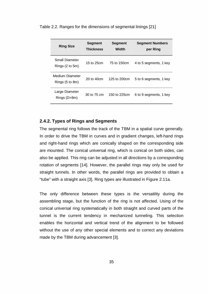
In addition to given dimensions of an ordinary TBM tunnel, ranges for the

dimensions of a segmental lining are given in Table 2.2. These values have

been obtained as a result of wide experiences. The geometrical pre-

dimensioning of a ring can be estimated with these ranges. Then, the pre-

dimensioning stage should be confirmed in the subsequent, more detailed

design stages.

35

Table 2.2. Ranges for the dimensions of segmental linings [21]

Ring Size Segment

Thickness Segment

Width Segment Numbers

per Ring

Small Diameter

Rings (2 to 5m) 15 to 25cm 75 to 150cm 4 to 5 segments, 1 key

Medium Diameter

Rings (5 to 8m) 20 to 40cm 125 to 200cm 5 to 6 segments, 1 key

Large Diameter

Rings (D>8m) 30 to 75 cm 150 to 225cm 6 to 9 segments, 1 key

2.4.2. Types of Rings and Segments The segmental ring follows the track of the TBM in a spatial curve generally.

In order to drive the TBM in curves and in gradient changes, left-hand rings

and right-hand rings which are conically shaped on the corresponding side

are mounted. The conical universal ring, which is conical on both sides, can

also be applied. This ring can be adjusted in all directions by a corresponding

rotation of segments [14]. However, the parallel rings may only be used for

straight tunnels. In other words, the parallel rings are provided to obtain a

“tube” with a straight axis [3]. Ring types are illustrated in Figure 2.11a.

The only difference between these types is the versatility during the

assembling stage, but the function of the ring is not affected. Using of the

conical universal ring systematically in both straight and curved parts of the

tunnel is the current tendency in mechanized tunneling. This selection

enables the horizontal and vertical trend of the alignment to be followed

without the use of any other special elements and to correct any deviations

made by the TBM during advancement [3].

36

In order to have a straight tunnel axis with conical universal ring, each ring

should be turned by 1800 in reference to the previous one. Using right ring

and left ring always enables to have the key segment on the top. By this way,

the ring is constructed from bottom to upwards [3].

Figure 2.11. Conicity of segmental rings: a) type of rings; b) relationship

between conicity and minimum radius of curvature of the tunnel

[14]

The relation between the conicity (C) of the ring and the minimum radius of

curvature (R) of the tunnel is determined by the formula given in the Figure

2.11b. Accordingly, C is directly proportional to the average ring width (W)

and inversely proportional to the radius R. For parallel rings (R→∞), the

conicity is C = 0.

37

It is necessary to understand the assembly process of the ring inside the tail

of the shield in order to choose the type of segment. The assembly process

involving the construction of the ring starts from the first segment, and

finishes up with the key segment, whose presence is always foreseen and is

placed at the opposite side of the ring that has the counter segment [3] (see

Figure 2.9).

The key segment has a shape of trapezoid with the largest side facing the

front of excavation. It is mostly smaller than all the other elements. For the

installation of key segment, two counter segments with inclined sides to

correspond with the shape of the key segment are necessary [3].

For the remaining part, segments may have any specific geometrical shapes

that are demonstrated in Figure 2.12. Apart from the honeycomb shape, the

others are all quadrilateral. All ring types can be built with segments having

suitable shapes shown below.

Figure 2.12. Segment types [17]

38

2.4.3. Segmental Lining Materials The main constituent materials of a segmental lining are concrete and

reinforcing steel. The Japanese Industrial Standard (JIS), Deutsche Industrie-

Norm (DIN), American Concrete Institute (ACI) Standard and Russian

Construction Norms and Regulations (SNIP) are the most widely used

standards in the design of lining concrete.

For the concrete of segmental linings, strength grade of at least C 35 is

demanded. Most segments are produced with quality C 40/50. Higher grades

are also available but not necessary in general. Depending on the

dimensions of the segments, and the support conditions, early strengths

ranging from 15 to 25 MPa may become necessary. Concrete used in the

production of segments should have several important properties, such as

workability, watertightness, high impact resistance, high flexural tensile

strength, and high resistance against aggressiveness of ground and

groundwater [21]. In addition to this, concrete making materials, cement,

aggregates, admixtures, and water should also comply with applicable

standards.

The reinforcement of a lining segment consists of the load bearing

reinforcement in circumferential and longitudinal direction, the tensile splitting

reinforcement adjacent to the longitudinal and circumferential joints, the

boundary reinforcement as well as the reinforcement for block outs and built-

in units. Generally, shear reinforcement is not required in segmental linings,

because the segments are loaded mainly by normal thrusts. However, it can

be installed in the form of stirrups or additional, ladder-shaped or S-shaped

rebars if needed.

The minimum yield strength of reinforcement to be used in segments should

be 420 N/mm2. Also, the reinforcement should be carried out with bars of not

more than 20 mm in diameter. If larger diameters are used, only small

39

imperfections of bending radii can lead to difficulties with fitting the

reinforcement cages into the formwork. As a result, the installation of

reinforcement becomes more complicated. Furthermore, the required

concrete cover is ensured by means of reinforcement bar spacers which are

generally attached to the reinforcement bars [14].

The various reinforcements of the segment are combined to a reinforcement

cage, which can be placed into the formwork completely (see Figure 2.13).

For this, the several rebars are welded together at single points. If required, a

mounting reinforcement has to be installed to fix the position of single bars.

Figure 2.13. Typical reinforcement cage for segmental linings

2.4.4. Contact Surfaces The proportion of joints in the tunnel tube is relatively high due to the

segmental building of the individual rings and the ring-wise production of the

lining. These are the longitudinal joints between the segments and the

circumferential joints between the adjacent rings. Longitudinal and

40

circumferential joints provide the transmission of axial forces, shear forces,

and moments between rings and segments.

2.4.4.1. Longitudinal (Segment) Joints

The longitudinal joints transfer axial forces, bending moment due to eccentric

axial forces, and shear forces from external and also sometimes internal

loading. From a statical point of view, the longitudinal joints are hinges with

restricted bearing capacity for bending moments (torsion springs). Bending

moments are transferred by eccentric forces acting in ring direction. Shear

forces are transferred by the friction which exists between the contact

surfaces of the joint.

There are three types of widely used longitudinal joints. These are:

• two flat surfaces

• two convex surfaces

• convex / concave surfaces

With longitudinal joints having two flat surfaces as shown in Figure 2.14a, the

free rotation of the segments is hindered by the geometry. Therefore, in

addition to the axial compression load in the longitudinal joint, bending

moments can also be transferred, which reduces the bending loading on the

segment [14].

Due to their small stiffness against torsion, joints with two convex surfaces

shown schematically in Figure 2.14b are suitable especially in case of high

compressive forces in connection with large angles of torsion between two

adjacent segments [13].

Longitudinal joints with convex / concave surfaces according to Figure 2.14c

normally have a high rotation capability. Therefore, this type of joint leads to

a better stability of the ring during assembly [13].

41

Figure 2.14. Longitudinal joints with a) two flat surfaces, b) two convex

surfaces, c) convex / concave surfaces [13]

In addition to these types, longitudinal joints with tongue and groove can be

mentioned as a possibility. However, it is not recommended for longitudinal

joints because the tongue cannot be reinforced and the concrete spalls off if

the play in the joint is only slightly exceeded.

A special form of tongue and groove joints has the one sided groove with

insert. This type is only used for smaller keystones in order to avoid them

falling out [13].

42

2.4.4.2. Circumferential (Ring) Joints

The ring joint level is positioned orthogonally to the tunnel’s longitudinal axis.

The thrust forces applied during construction are transferred through the

circumferential joints. Due to adjacent rings having different deformation

patterns, coupling forces (transverse forces) are created in the ring joints

when the deformation is hindered [13]. In the circumferential joints, load

transmission pads consisting of hardboard (timber sandwich layers) or

“Kaubit” (caoutchouc and bitumen) are arranged to compensate for mounting

tolerances and to assure the load transfer at predetermined surfaces [14].

The most common forms of ring joints can be listed as follows:

• flat ring joints

• tongue-and-groove systems

• cam-and-pocket systems

The flat ring joints shown in Figure 2.15 are the simplest form of ring joints.

Each ring joints of this type supports itself without interacting with adjacent

rings, or at least not intentionally. The coupling is only through friction.

Transverse load transfer through joint is not intended. However, this can be

implemented for small coupling forces with a durable bolted connection (see

Figure 2.15).

To simplify the installation of the ring and to establish a force transmitting

connection of adjacent rings during machine tunneling in the ground, the

circumferential joints are equipped with tongue-and-groove systems or cam-

and-pocket systems. The coupling avoids large relative displacements

between adjacent rings and leads to an increase of the flexural stiffness of

the segmental lining [14].

The relative displacements of adjacent rings are very small during the TBM

tunneling in rock. Therefore, remarkable coupling forces do not occur.

43

Accordingly, circumferential joints with flat surfaces are usually carried out for

segmental linings in rock.

Figure 2.15. Circumferential joint with flat surfaces [14]

In a tongue-and-groove system as shown in Figure 2.16, the tongue is mostly

wider than half of the segment's width and has a height of 10 to 30 mm. This

flat toothing can not be reinforced for bearing the coupling forces, if the

required concrete cover is obeyed. The usually inevitable assembly

inaccuracies and the resulting constraints often lead to damages during

machine tunneling in soil. To minimize this damage, the groove is made

larger than the tongue. The available play usually reaches upto a few

millimeters and is quickly eaten up by manufacturing and installation

tolerances [14].

44

Figure 2.16. Circumferential joint with tongue-and-groove system [14]

In a cam-and-pocket system as shown in Figure 2.17, the constraints due to

assembly inaccuracies are limited to the cam-and-pocket area. In case of a

deep toothing with a correspondingly high cam, the cam can also be

adequately reinforced. Also, the height of the cam should be selected so that

a failure would occur at the cam and not shear off the edge of the pocket,

then the waterproofing is preserved.

Using a tongue-and-groove system or a cam-and-pocket system, the

coupling forces are transferred through load transmission pads (coupling

pads) consisting of "Kaubit" instead of direct contact of concrete.

In addition to these types, convex – concave designs of the ring joint are also

known. However, the edge surfaces of concave faces are at risk of damage

during assembly.

45

Figure 2.17. Circumferential joint with cam-and-pocket system [14]

2.4.5. Connectors Connectors are used to hold segments and rings together until the grout

material hardens and the segment or ring is fixed in its final position. For the

connections between segments and rings, two types of connectors are used

in general:

a) Joints with bolts: the segment is first placed in position and then the

bolts are inserted and tightened. This type requires effort in the construction

46

of the mould because it is necessary to create “pockets” and “grooves” into

which the bolts are inserted. Also, more staff is required to insert the bolts.

This type is mostly used both between rings and between segments, within a

ring [3].

The bolts are metallic while the embedded threads are generally plastic.

Figure 2.18 shows the typical housing of a straight bolt.

Figure 2.18. Section of a typical housing for a single bolt [3]

Bolts with curved elements also exist, but not common. However, the details

about the geometry of straight elements are fundamentally valid in this case.

b) Joints with dowels: the connectors, which are completely covered and

hidden, are inserted into the segment during the assemblage and are

mortise-inserted into the segment of the last assembled ring.

Since the insertion is automatically performed by the erector when the

segment is positioned, this type of connector requires less work for

construction of the mould and less manpower in the tunnel [3].

47

The dowels and nuts are made of plastic and sometimes have the core in

steel. Figure 2.19 shows the typical housing of a pin for the variety with a nut

and without a nut, in which the pin is directly forced into a hole cut out of the

concrete.

Figure 2.19. Section of a typical room for a single dowel [3]

The connection with dowels can be used only for rhomboidal and/or

trapezoidal segments to avoid early crawling of the gaskets during the ring

assembly [3].

Differently from dowels, screwings of bolts are released and bolts are

removed as soon as the restoring forces of the gaskets can be transmitted by

the annular gap grouting into the rock mass and an influence of the jacking

forces does not exist anymore. For this purpose, the bolts should be removed

after the gap grouting has set. However, in the area of portals and cross cuts,

the screwing of bolts are permanent because the shearing bond between the

annular gap grouting, the segmental lining and the rock mass may not be

sufficient to carry the restoring forces of the gaskets. Furthermore, corrosion-

resistant screws should be used in these regions [14].

48

2.4.6. Waterproofing System Waterproofing of a ring is generally provided by the following equally

important factors [3]:

• an optimal quality of the concrete and of the segment, resulting from

the high level strength of the concrete used together with an accurate

prefabrication process,

• provision of care when moving the individual segments to avoid the

formation of cracks,

• choice and positioning of gaskets,

• proper assembly of ring, aligning the segments, and avoiding any

possible damage,

• filling the annular gap with suitable material.

The sealing elements always work in pairs because they are placed in

special grooves embedded on each side of all the segments close to the

extrados and they come into contact when the segments are assembled to

form a ring. There are mainly two types of gaskets:

a) Compression Gaskets: watertightness is ensured by the compression of

gaskets. The compressive stress is ensured by the connectors (for both ring

and segments) in the short term and by stresses acting in the ring in the long

term [3].

b) Compression and Swelling Gaskets: working principle is basically the

same with compression gaskets. In addition to compression, this type of

gasket physically swells in the presence of water and develops a very high-

pressure sealing capacity [3]. All of gaskets have nearly similar geometries

and are only different in terms of their width, height, and hardness of rubber

(EPDM) from which gasket is made.

49

2.4.7. Ring Assembly Ring assembly process starts with the supply of the segments at the portal

and finishes with the exit of the ring from the tail of the TBM. The segments

are transported by wagons that move either on wheels or tracks. Wagons

carry the segments into the back-up where they are lifted by a system known

as “segment feeder” which takes them to the erector positioned inside the

shield. For straight tunnels, the arrival order is arranged according to

assembling order of segments. In order to prevent any confusion about

ordering, the segments are marked with letters and/or numbers that

determine the assembling sequence [3].

Before the installation of a new segmental ring, the previously mounted ring

should be inspected. Fractured or cracked segments should be dismounted

and replaced by new and sound segments. The tail-skin should be clean and

dry also at the invert.

Ordinarily, the first segment is attached to invert of the ring mounted before.

When positioned correctly by the erector, the segment is pushed against the

previously mounted ring by the thrust cylinders as shown in Figure 2.20.

Subsequently, the screwings in the circumferential joints are fixed. After all

screws are fixed and prestressed respectively, the erector can be retracted

from the segment.

Then, the following segments are alternatively installed to left or right of the

first segment. The longitudinal joints should be completely closed. If the

installation is not done properly, longitudinal joints are compressed by the

annular grout after the ring assembly is completed. This may lead to

damages to the segments on the outside of the ring.

50

Figure 2.20. Installation of segments and transmission of thrust forces into

the segmental linings [14]

Before the installation of key segment, it should be checked if there is

enough space between the counter segments for mounting the keystone. If

there is not enough space, the ring should be dismantled and erected again.

The key segment is installed with the erector far enough to create the

required prestressing of gaskets in the circumferential joints. The jacks of the

adjacent segments are slightly retracted to avoid restraints in order to install

the keystone completely. Afterwards, the thrust cylinders are only pushed

again when the screws in the longitudinal joints are completely fixed [14].

As mentioned above, circumferential and longitudinal connections are mostly

fixed with bolts for the installation of segmental ring and to secure the

geometry. Generally, the screw connections are removed after imbedding the

51

ring in the grout. Then, a bolted connection is no longer necessary, because

the longitudinal joints are pressed into place by the ground pressure and

water pressure; and pre-loads are present in the ring joints created by

resetting forces of the sealing section [22].

52

CHAPTER 3

LITERATURE REVIEW

In this chapter, a brief literature review of TBM segmental lining analysis

methods is provided along with recent published literature. Selected analysis

methods (elastic equation method and beam – spring method) which will be

evaluated in this project are explained and discussed in more detail.

3.1. Analysis Types Structural methods used to analyze TBM segmental linings must be able to

indicate loads and deformations in accordance with the geologic and

construction conditions and also represent the ground – lining interaction.

There are various structural methods that satisfy these criteria. They include

estimations based on empirical evidence, analytical solutions, and numerical

simulations. General tendency for calculating the member forces of the TBM

segmental lining is to perform numerical simulation. However, analytical

methods are also commonly used to provide a collective check on the

results. According to ITA – WG2 [23], the member forces should be

computed by using belowmentioned methods:

• Elastic Equation Method

• Schulze and Duddeck Model

• Muir Wood Model

• Beam – Spring Method

• Finite Element Method

53

There is no unique solution in tunnel engineering. All of these methods have

strengths and weaknesses. Also, each method mentioned above has some

limitations that restrict the usage of them. For that reason, strengths,

weaknesses, and limitations of the methods should be investigated in detail

before selecting the proper method to be used in design.

This thesis study mainly focuses on beam – spring method, but elastic

equation method is also examined as an analytical approach. Therefore, this

chapter particularly describes elastic equation method and beam – spring

method in detail. Also, other methods are briefly mentioned.

3.1.1. Elastic Equation Method The elastic equation method, also called as usual calculation method, is a

simple method for calculating member forces of circular tunnels without a

computer. This method is proposed by Japanese Standard for Shield

Tunnelling [24] and has been widely used in Japan. Key points of this method

are provided in this section.

Load distribution model used for this method is shown in Figure 3.1. In the

figure, P0 is overload (surcharge); R0 is the external radius of shield lining; Rc

is the radius of middle line of shield lining; g is gravity of lining; Pe1 and Pw1

are, respectively, the vertical earth pressure and water pressure acted on the

up side of shield lining. The lateral earth pressure and water pressure vary

linearly and act on both sides of the shield lining. They are equal to qe1 and

qw1 at the top of the shield lining, and qe2 and qw2 at the bottom of shield

lining; Pe2 and Pw2 are respectively the vertical earth pressure and water

pressure acted on the bottom side of shield lining; Pg is the vertical

resistance of lining weight acted on the bottom side of shield lining.

For sandy clay, the earth pressure and water pressure are assumed to act on

the lining separately. If the overburden thickness is two times larger than the

54

external diameter D of shield lining (h0 ≥ 2D), an effective overburden

thickness h0 should be used and it can be determined by Terzaghi’s formula

described in Chapter 4.3.4.

The distribution of horizontal earth resistance has a triangular shape and its

application range is shown in Figure 3.1.

Figure 3.1. Load condition of Elastic Equation Method [24]

55

After having all parameters determined, the internal forces of the segmental

lining can easily be computed. Elastic formulas for the calculation of member

forces are given in Table 3.1.

Table 3.1. Equations of member forces for Elastic Equation Method [24]

Load Bending Moment Axial Force Shear Force

Vertical Load

(P= pe1+pw1) (1-2S2)*P*Rc

2/4 S2*Rc*P -SC*Rc*P

Horizontal Load

(Q= qe1+qw1) (1-2C2)*Q* Rc

2/4 C2*Rc*Q -SC*Rc*Q

Horizontal

Triangular Load

(Q’= qe2+qw2

-qe1-qw1)

(6-3C-12C2+4C3)*Q’*

Rc2/48

(C+8C2-4C3)*

Q’*Rc/16

(S+8SC-4SC2)*

Q’*Rc/16

Soil Reaction

(Pk= k.δh)

0≤θ≤π/4

(0.2346-0.3536C)*

Rc2*kδ

π/4≤θ≤π

(-0.3487+0.5S2+

0.2357C3)*Rc2*kδ

0≤θ≤π/4

0.3536C*Rc*kδ

π/4≤θ≤π

(-0.7071C+C2+

0.7071S2C)*Rc*kδ

0≤θ≤π/4

0.3536S*Rc*kδ

π/4≤θ≤π

(SC-0.7071C2S)*

Rc*kδ

Dead Load

(Pg= π.g)

0≤θ≤π/2

(3/8π-θ*S-5/6C)*Rc2*g

π/2≤θ≤π

[-π/8+(π- θ)S-5/6C-

1/2π*S2]*Rc2*g

0≤θ≤π/2

(θ*S-1/6C)*Rc*g

π/2≤θ≤π

(-π*S+θ*S+ π*S2-

1/6C)*Rc*g

0≤θ≤π/2

(θ*C-1/6S)*Rc*g

π/2≤θ≤π

[-(π-θ)*C+θ*S+

π*SC-1/6S]*Rc*g

Horizontal

Deformation at

Spring Line (δh)

δh= [(2P-Q’)+π*g]* Rc4/[24*(EI/h+0.045k* Rc

4]

θ= angle from crown, S= sin θ, S2= sin2 θ, S3= sin3 θ, C= cos θ, C2= cos2 θ, C3= cos3 θ

56

Segmental ring is composed of several segments which are connected by

bolts or dowels. The deformation at these connection joints is larger than the

one in a ring with uniform rigidity, because the rigidity of joints is less than the

rigidity of segment section. Furthermore, the connections at the segment

joints are generally staggered. However, this method assumes the segmental

ring with uniform bending rigidity and can not represent the staggered

geometry [24]. Nevertheless, the solutions obtained by this method can be

very practical and helpful for checking the results obtained by numerical

methods [2]. Also, this method is mostly used in preliminary design and cost

estimation for a new tunnel project.

This method is more advantageous than other closed form solutions,

because elastic equation method has a capability of calculating bending

moment, axial force, and shear force of any point on the lining. However,

other closed form solutions can only determine the bending moments and

hoop forces at the point where relative maximum values occur.

3.1.2. Schulze and Duddeck Method The thrust and bending moment in circular linings surrounded by an elastic

medium can be determined by several closed form solutions such as Schulze

and Duddeck Method. These closed form solutions deal only with tunneling

models for soft ground and the some basic assumptions are applied to derive

a model such that the cross-section is circular, the material behavior of

ground and lining is elastic, the active soil pressures on the lining are taken

as equal to the primary stresses in the undisturbed ground, and there exists a

bond between the lining and the ground for radial and tangential

deformations [25].

The complete and closed solutions for the model (Figure 3.2) intended for

shallow tunnels (H ≤ 6R) limited overburden is published by Schulze and

Duddeck [26] in 1964. Surrounding ground is represented by ground springs.

57

Since tension springs may cause load reduction, bedding at the crown is

omitted. The results of this study is given as direct design diagrams for

bending moments, hoop forces, and radial displacements for those three

points of the lining where relative maximum values occur. In this method,

modulus of subgrade reaction (Kr) is a free parameter and the tangential

stresses may be included in or omitted from the load parameters [25].

Figure 3.2. Bedded ring model without crown bedding [25]

3.1.3. Muir Wood Method Muir Wood Method is another closed form solution used to determine hoop

forces, bending moments, and radial displacements. Like most closed form

solutions, this model is based on the assumption that the ground is an

infinite, elastic, homogeneous, and isotropic medium. Also, the basic

assumptions for closed form solutions determined in the previous section are

valid for this method.

Muir Wood model [27] is based on plain strain continuum model shown in

Figure 3.3. This method assumes that the circular lining deforms into an

elliptical mode. The tangential ground stresses are included, but radial

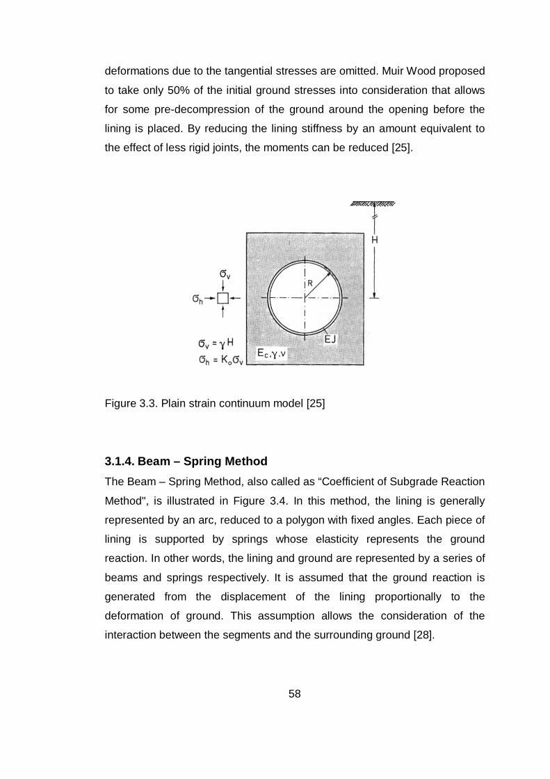
58

deformations due to the tangential stresses are omitted. Muir Wood proposed

to take only 50% of the initial ground stresses into consideration that allows

for some pre-decompression of the ground around the opening before the

lining is placed. By reducing the lining stiffness by an amount equivalent to

the effect of less rigid joints, the moments can be reduced [25].

Figure 3.3. Plain strain continuum model [25]

3.1.4. Beam – Spring Method The Beam – Spring Method, also called as “Coefficient of Subgrade Reaction

Method", is illustrated in Figure 3.4. In this method, the lining is generally

represented by an arc, reduced to a polygon with fixed angles. Each piece of

lining is supported by springs whose elasticity represents the ground

reaction. In other words, the lining and ground are represented by a series of

beams and springs respectively. It is assumed that the ground reaction is

generated from the displacement of the lining proportionally to the

deformation of ground. This assumption allows the consideration of the

interaction between the segments and the surrounding ground [28].

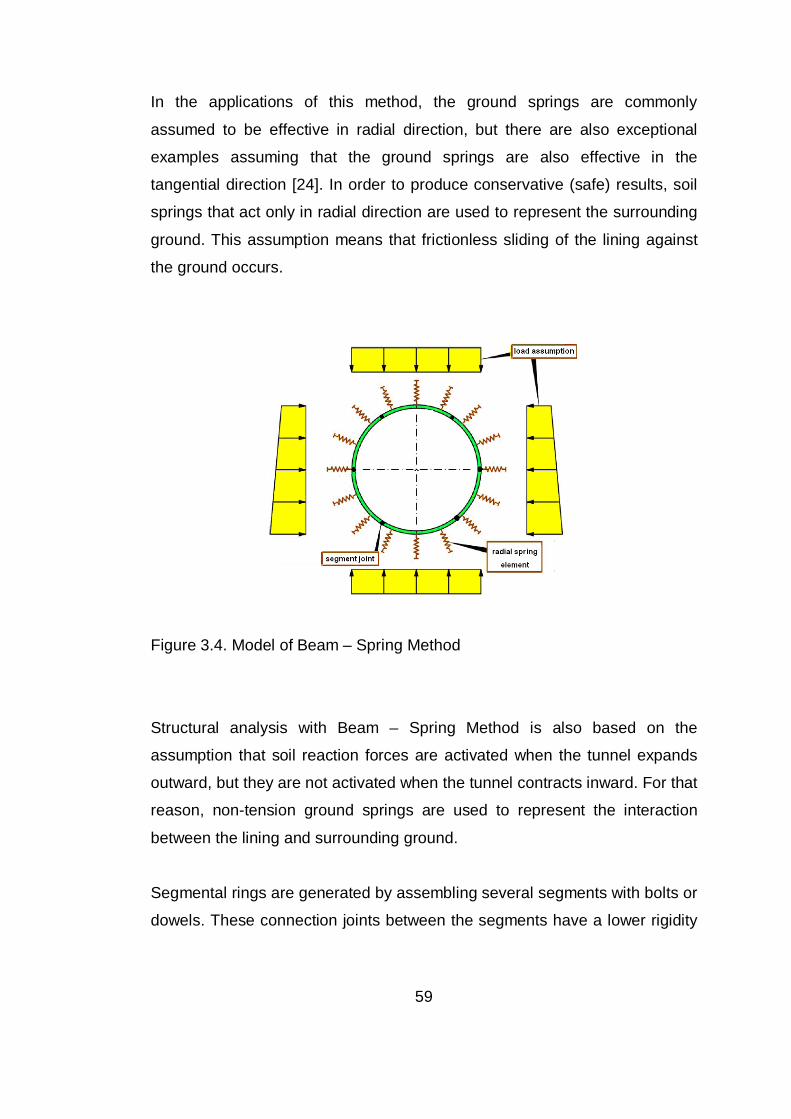
59

In the applications of this method, the ground springs are commonly

assumed to be effective in radial direction, but there are also exceptional

examples assuming that the ground springs are also effective in the

tangential direction [24]. In order to produce conservative (safe) results, soil

springs that act only in radial direction are used to represent the surrounding

ground. This assumption means that frictionless sliding of the lining against

the ground occurs.

Figure 3.4. Model of Beam – Spring Method

Structural analysis with Beam – Spring Method is also based on the

assumption that soil reaction forces are activated when the tunnel expands

outward, but they are not activated when the tunnel contracts inward. For that

reason, non-tension ground springs are used to represent the interaction

between the lining and surrounding ground.

Segmental rings are generated by assembling several segments with bolts or

dowels. These connection joints between the segments have a lower rigidity

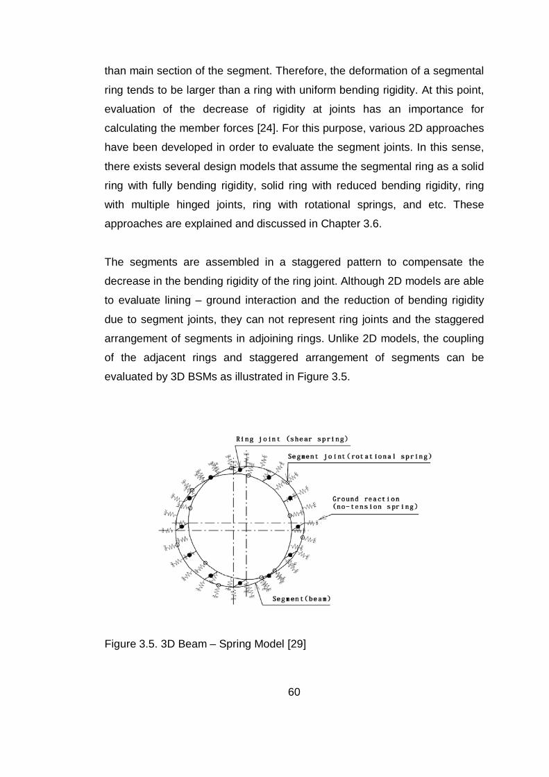
60

than main section of the segment. Therefore, the deformation of a segmental

ring tends to be larger than a ring with uniform bending rigidity. At this point,

evaluation of the decrease of rigidity at joints has an importance for

calculating the member forces [24]. For this purpose, various 2D approaches

have been developed in order to evaluate the segment joints. In this sense,

there exists several design models that assume the segmental ring as a solid

ring with fully bending rigidity, solid ring with reduced bending rigidity, ring

with multiple hinged joints, ring with rotational springs, and etc. These

approaches are explained and discussed in Chapter 3.6.

The segments are assembled in a staggered pattern to compensate the

decrease in the bending rigidity of the ring joint. Although 2D models are able

to evaluate lining – ground interaction and the reduction of bending rigidity

due to segment joints, they can not represent ring joints and the staggered

arrangement of segments in adjoining rings. Unlike 2D models, the coupling

of the adjacent rings and staggered arrangement of segments can be

evaluated by 3D BSMs as illustrated in Figure 3.5.

Figure 3.5. 3D Beam – Spring Model [29]

61

As shown in Figure 3.5, this 3D model has an ability to evaluate the reduction

of bending rigidity and splice effects of staggered geometry by using a model

in which a segment is considered as a curved or straight beam, a segment

joint as a rotational spring, and a ring joint as a shear spring. Like 2D model,

ground reaction is represented by non-tension springs. In addition, minimum

two or more rings are used in the 3D analysis in order to evaluate the

coupling of rings, the effect of joint locations and combinations, and shear

stresses on a ring joint [24].

Design procedure, design stages, loading types and conditions, and

structural calculation used in the design of segmental linings are briefly

discussed in Chapter 4.

3.1.5. Finite Element Method Finite Element Method (FEM) which is illustrated in Figure 3.6 is one of the

most widely used numerical methods in geomechanics. It is a continuum

model but discontinuities can also be modeled individually. In FEM, the

hosting ground is discretized into a limited number of smaller elements.

These elements are connected at nodal points. The stress, strain, and

deformation to be analyzed are caused by changing the original subsurface

conditions. For instance, such change might be induced by tunneling

process. The stresses and strains generated in one element effects the

interconnected elements, and so forth [6].

The stress-strain relationships of the elements are modeled mathematically

by creating a global stiffness matrix which relates the unknown quantities

with known quantities. Then, this matrix is solved using standard matrix

reduction techniques and the results are obtained. The equations to be

solved are highly complicated, and as the number of the elements in the

model increase, the calculation time and the storage capacity increase

dramatically.

62

By means of FEM, complex underground conditions and tunnel

characteristics can be analyzed. Furthermore, this method enables the

simulation of complex constitutive laws, non-homogeneities, and the impact

of advance and time dependent characteristics of the construction methods.

Figure 3.6. Finite element method for tunnel engineering

On the other hand, most FEM programs require more knowledge on program

and computer than other methods do. Typically the output of the analysis is

also complex and it becomes difficult to assess the results. Therefore, a post-

processor may be utilized in order to overcome this difficulty [6].

3.2. Theoretical Approaches on Beam – Spring Method Since Beam – Spring Method is the most effective and practical tool for the

calculation of member forces of TBM segmental linings, several theoretical

approaches have been developed in this field. The main determinant criteria

in BSMs are the ground lining interaction and connection joints. For ground

lining interaction, most approaches employ non-tension elastic ground

63

springs. However, these approaches have different methods to evaluate

connection joints. Therefore, these theoretical approaches can be classified

by joint evaluations.

Selecting the proper structural model in order to calculate the member forces

of TBM segmental linings should be done carefully, because it depends on

several conditions, such as usage of tunnel, design loads, geometry and

arrangement of segments, ground conditions, and required accuracy of

analysis. Schematic drawings of structural models outlined by JSCE [24] are

illustrated in Figure 3.7.

Figure 3.7. Structural design models for TBM segmental linings

64

Available structural models in the literature are summarized in Figure 3.7. 2D

models (I-IV) are able to represent only segment joints by using reduced

rigidity, hinges, or rotational springs. However, 3D models (V-VI) can

simulate both segment joints and ring joints. In 3D models, segment joints

are represented by rotational springs, and ring joints are modeled as rigid

members or shear springs.

The common part of these BSMs is the ground – lining interaction. It is

simulated by non-tension elastic ground springs in radial direction as shown

in Figure 3.4 and Figure 3.5. The soil spring constant is calculated using the

following theoretical formulas proposed by Muir Wood, in accordance with

AFTES – WG7 Appendix 1 [28].

( ) REk⋅+

=υ1

(3.1)

where, k : Modulus of subgrade reaction of the ground in the radial

direction (kN/m3),

E : Modulus of deformation of ground (kN/m2),

υ : Poisson’s ratio,

R : Outer radius of segment (m).

wlkAkk str ⋅⋅=⋅= (3.2)

where, kr : Soil spring constant in the radial direction (kN/m),

k : Modulus of subgrade reaction of the ground in the radial

direction (kN/m3),

At : Tributary area (m2),

sl : Distance between soil springs (m),

w : Width of segment (m).

65

Structural models given in Figure 3.5 are sorted from the simplest one to the

most complicated one, and also show the development of the approaches.

After the conditions of tunnel project are denoted, structural calculations of

segmental linings can be performed by a single model. In order to decide on

the proper model, all models should be investigated.

In Model I, the segmental ring is assumed to be a ring with uniform bending

rigidity. The decrease of rigidity at segment joints is ignored and a segmental

ring is treated as a ring with uniform bending stiffness EI as a main section of

a segment [24]. In other words, this model can be named as “solid ring with

fully bending rigidity”. This is the simplest 2D model and can not evaluate the

connection joints. Therefore, this model gives more conservative results than

the others.

In Model II, the segmental ring is again assumed to be a ring with uniform

bending rigidity, but bending rigidity is reduced in order to simulate the effects

of segment joints. There are different approaches for the reduction of

bending rigidity.

Bickel, Kuesel, and King [30] have proposed a 2D model that simulates the

segment joints by using reduced stiffness parameters. This model assumes

that the stiffness (effective modulus of elasticity) of a segmental ring is half

that of a monolithic ring and the moment of inertia of practical coffered

precast segments ranges from 60 to 80% of that of solid sections with the

same thickness. Due to reduced stiffness, this model is more flexible than

Model I and expected to give less values for bending moment and hoop

forces.

Furthermore, Koyama and Nishimura [31] have recommended a model in a

similar manner with the former model proposed by Bickel, Kuesel, and King.

According to these Japanese researchers, the tunnel lining is assumed to be

66

a continuous ring with a discounted rigidity by applying a reduction factor, η,

to the bending rigidity (EI) of the tunnel lining. Koyama and Nishimura [31]

suggested determining η by full ring structural testing. If experimental data

are not available, the value of η can be assumed to be in the range of 0.6 –

1.0 for preliminary design analysis. For instance, a continuous monolithic ring

beam having a constant effective rigidity ratio of η= 0.8 was used in the

design of the Trans-Tokyo Bay Highway tunnel lining (Uchida 1992). The

value of η adopted in the tunnel project was later verified by tests on a full-

scale prototype segmental lining [32].

Muir wood [27] investigated the effects of joints between the segments and

proposed an easy to use empirical formula to estimate the effects of the

longitudinal joints of rings in a calculation with a homogeneous rigid ring by

reducing the bending stiffness of the lining. The effective moment of inertia,

Ie, for a segmental tunnel ring with a number of equal segments can be

expressed as follows.

In

II je ⋅

+=

24 Ie ≤ I, n > 4 (3.3)

where, Ie : The effective moment of inertia,

Ij : The moment of inertia at the force transmission zone

between the joints,

I : The moment of inertia of the lining section,

N : Number of segments (key segment not counted).

Muir Wood [27] suggested that the existence of segment joints would not

affect the rigidity of the lining for four or fewer lining segments. The earth

pressure acting around a tunnel is assumed to be in an elliptical shape in this

model. In order to obtain this elliptical shape for initial loading, sufficient

overburden thickness is required. Therefore, Muir Wood model is more

67

convenient for deep tunnels. This assumption may not be valid for shallow

tunnels.

First two approaches given for Model II make some assumptions for the

effect of segment joints. However, the effects of the number of segments are

not considered. Although Muir Wood model takes into consideration the

number of segments, it can not simulate joint orientation. According to

numerical studies done by Hefny, Tan, and Macalevey [33], the values of

moments induced in the lining are reduced by 8 times by orientating the joints

with an angle of 45°. This shows that in addition to the number of segment

joints, the orientation of joints also affects the member forces considerably.

Since these effects may lead to large reduction in costs, they should be

conceived.

Model III assumes the segmental ring as a ring having several hinges. This

model is used in United Kingdom and Russia, where ground conditions are

relatively good i.e. hard rock. In this model, segment joints are modeled as

unfixed hinges. Afterwards, deformation is calculated and checked for safety.

This model gives considerably less bending moments and leads to more

economical design for the grounds in good condition. Since this method fairly

depends on ground conditions, adequate study should be done in order to

determine whether the model is suitable for the existing ground or not [24].

Model IV simulates not only the number of segment joints but also the joint

orientation. Segment joints are modeled as rotational springs as illustrated in

Figure 3.8a. The crucial point for this model is the calculation of rotational

spring constant. For the behavior of rotational stiffness of longitudinal joints,

worldwide accepted formulas proposed by Janssen [34] based on the

investigation of Leonhardt and Reimann [35] for the resistance against

rotation and bending of concrete hinges are used.

68

Figure 3.8. a) Rotational spring model, b) Stress distribution at the segment

joint [37]

While developing the theoretical formula of Leonhardt and Reimann

concerning concrete joints, the following assumptions are made on the basis

of fundamental experimental results and observations concerning concrete

joints.

• Tensile stress is not transmitted at joints.

• Compression stress has linear distribution.

• The deformation coefficient is constant, having the magnitude of E0,

the initial connection elasticity coefficient in σ = ε = 0.

• The scope of deformation in the acting direction of axial force is

centered on the joint surface, and limited to the same scope as the

width of the convex potion of the joint. Strain is distributed uniformly.

The theoretical formulas based on the above assumptions and the geometric

relationships are developed as follows and shown in Figure 3.9.

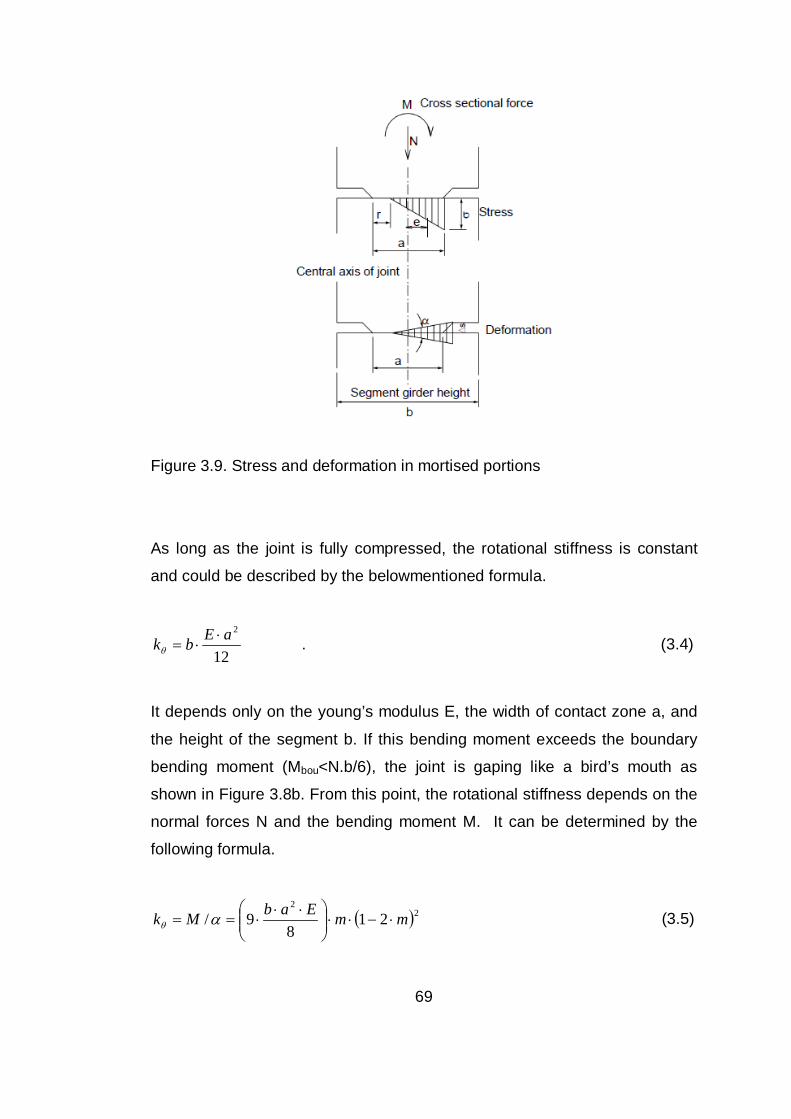
69

Figure 3.9. Stress and deformation in mortised portions

As long as the joint is fully compressed, the rotational stiffness is constant

and could be described by the belowmentioned formula.

12

2aEbk ⋅⋅=θ . (3.4)

It depends only on the young’s modulus E, the width of contact zone a, and

the height of the segment b. If this bending moment exceeds the boundary

bending moment (Mbou<N.b/6), the joint is gaping like a bird’s mouth as

shown in Figure 3.8b. From this point, the rotational stiffness depends on the

normal forces N and the bending moment M. It can be determined by the

following formula.

( )22

218

9/ mmEabMk ⋅−⋅⋅

⋅⋅⋅== αθ (3.5)

70

where θk : Rotational spring constant of joint (kN.m/rad)

α : Rotational angle (rad)

M : Bending moment (kN.m)

M : Load eccentricity rate, m = e/a = M / (N.a)

N : Axial force (kN)

B : Contact zone (mortise) length (m)

A : Contact zone (mortise) width (m)

E : Young’s modulus of concrete (kN/m2)

In order to employ this behavior, the above mentioned relationship between

bending moment and rotational stiffness should be performed by non-linear

rotational springs. Since rotational springs become extremely soft if the

moment increases to more than about 80 % of the maximum moment, it is

not necessary to define a yielding moment. Therefore, if only a linear

rotational spring with the definition of a yielding moment is modeled, the

simulation of behavior of segment joint seems to be very poor [36].

Model V, a 3D beam – spring model, is proposed by Koyama [38]. This

model simulates the segment joints as rotational spring like model IV and

supposes a rigid connection between the rings by using rigid members. It is

assumed that the displacement of the ring beam is equal to that of the

neighboring ring beam at the joint. Therefore, no gap occurs due to the shear

stress. However, relative displacement between the two neighboring rings

occurs in the longitudinal direction, and is concentrated at the centerline of

the segmental rings [39].

Model VI, also proposed by Koyama [38], is an advanced version of model

V. Differently from Model V, connection between the rings is modeled as

shear springs. Calculation of shear spring constant is a complex issue

because it depends on many factors such as type of ring joint (flat, cam-and-

pocket, tongue-and-groove), type of connectors (bolt, dowel), number, and

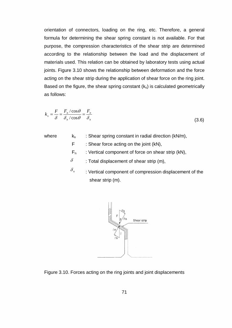
71

orientation of connectors, loading on the ring, etc. Therefore, a general

formula for determining the shear spring constant is not available. For that

purpose, the compression characteristics of the shear strip are determined

according to the relationship between the load and the displacement of

materials used. This relation can be obtained by laboratory tests using actual

joints. Figure 3.10 shows the relationship between deformation and the force

acting on the shear strip during the application of shear force on the ring joint.

Based on the figure, the shear spring constant (ks) is calculated geometrically

as follows:

n

n

n

ns

FFFkδθδ

θδ

===cos/cos/

(3.6)

where ks : Shear spring constant in radial direction (kN/m),

F : Shear force acting on the joint (kN),

Fn : Vertical component of force on shear strip (kN),

δ : Total displacement of shear strip (m),

nδ : Vertical component of compression displacement of the

shear strip (m).

Figure 3.10. Forces acting on the ring joints and joint displacements

72

For the 3D analysis of segmental rings, the shear spring constant is generally

obtained by laboratory tests or by experience of other comparable projects.

However, if flat (plate) ring joints with plywood hardboards are used, the

following formula for the shear stiffness of plywood can be used to determine

shear spring constant [36].

dAGks⋅

= (3.7)

where ks : Shear spring constant in radial direction (kN/m),

G : Shear modulus of plywood (kN/m2),

A : Area of hardboard (m2),

D : Thickness of hardboard (m).

Among the models in scope, this model is the unique one that can simulate

the interaction between adjacent rings. If spring constants are calculated

properly, the most realistic results can be obtained with this model.

3.3. 2D and 3D Analysis of TBM Segmental Linings Tunneling is a 3D problem where structural behavior of tunnel in the

longitudinal direction and the analysis of loads during and after the

construction may play an important role in the design of tunnels. Numerical

methods in tunnel engineering have been widely used with a steady growth

since the early applications in the mid 1960’s. This is most probably due to

the fact that numerical methods are capable of simulating the excavation,

construction, and service steps. In contrast with analytical solutions, these

are the distinctive advantages for numerical methods [40].

Although 3D numerical analysis of tunnels can simulate the structural

behavior of tunnel in the longitudinal direction and construction process, 2D

numerical studies in tunneling are much more popular than the 3D analysis.

73

2D analyses assume plane-strain conditions for the lining and ground. This

leads to avoiding three-dimensional effects. This type of simplifications made

by performing 2D numerical analysis make the calculations easier and less

time consuming, but they are not able to simulate 3D effects. In other words,

2D numerical methods are suitable for some cases, but they are not as

accurate as 3D models. For that reason, it is crucial to identify which

situations are convenient for 2D or 3D analysis. Consequently, the aim of this

study is to evaluate available analysis methods (analytical, 2D and 3D

numerical) for TBM segmental lining and propose suitable type of analysis for

certain situations.

Blom at al. [41] investigated the stresses due to tunnel excavation by

implementing 3D finite element model analyses for shield-driven Green Heart

Tunnel. They have also compared the results obtained by 3D finite element

analyses with analytical method (Schulze and Duddeck Model) and on-site

measurements. This study showed that the results of 3D finite element model

were so consistent with values obtained by on-site measurements, and 3D

analysis simulated the stress distribution realistically. However, sectional

forces predicted by analytical model did not fit well to on-site measurements.

It can be concluded that 3D finite element models simulate the stresses and

structural behavior of tunnels much more realistically than conventional

methods.

Klappers at al. [36] made a comparison between 3D Beam – Spring Method

and 3D FEM analysis with shell elements. This comparison showed that the

calculated sectional forces of both models were more or less the same, and

also only deformations differed slightly. This means that 3D FEM calculations

are not necessary for normal loading conditions. For special cases like

openings in the lining, different loads on the rings or varying bedding

conditions, 3D FEM modeling is needed to calculate internal forces and

deformations.

74

Mashimo and Ishumura [29] investigated loads acting on the shield tunnel

lining by using 3D BSM. This study also revealed that 3D BSM gives realistic

results if loading conditions and spring constants are calculated accurately.

Previous studies showed that 3D Beam – Spring Method is a useful tool in

order to obtain sectional forces of TBM segmental linings. In this thesis study,

an analytical method (elastic equation method), 2D beam – spring methods

with different approaches and 3D beam – spring method will be evaluated

and validity of methods for certain situations will be determined.

75

CHAPTER 4

TBM SEGMENTAL LINING DESIGN

Segmental linings are commonly used form of lining particularly for relatively

long tunnels where using a TBM is advantageous in terms of economy.

Design of a segmental linings not only requires structural analysis for the

ground loads and the TBM ram loads applied to segments, but it also

requires the designer to consider the total process of manufacture, storage,

delivery, handling, and erection as well as the stresses caused by sealing

systems and bolts.

Tunneling as an engineering discipline is unique. It has relied mainly on

experience and most segmental lining designers came from a structural

engineering background. The general approach for the design of segmental

lining is to estimate, as accurately as, the magnitude and distributions of

loads applied to tunnel support system and then detail the lining to carry the

loads [42]. A proper design can be performed by following a progressive

procedure taking into consideration all conditions of the problem.

This chapter typically indicates the design procedure, loading conditions, and

structural calculation procedure used in the design of segmental tunnel

linings. In the scope of this study, all structural analysis models are

performed in accordance with these procedures.

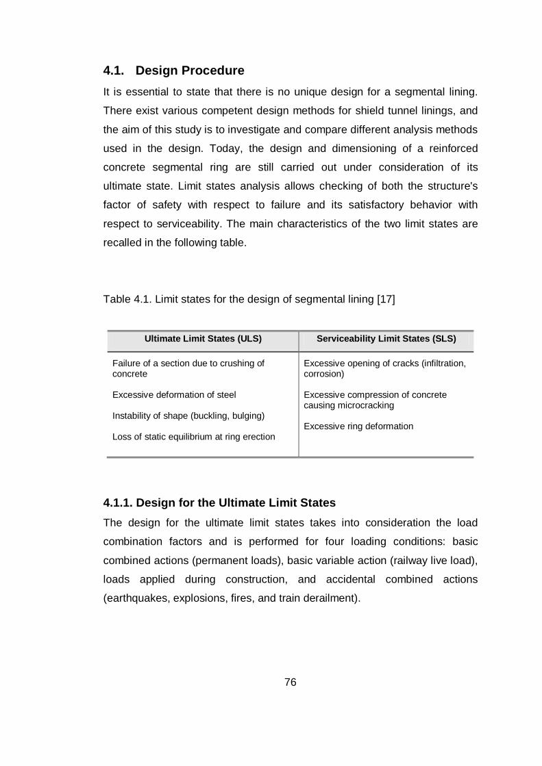
76

4.1. Design Procedure It is essential to state that there is no unique design for a segmental lining.

There exist various competent design methods for shield tunnel linings, and

the aim of this study is to investigate and compare different analysis methods

used in the design. Today, the design and dimensioning of a reinforced

concrete segmental ring are still carried out under consideration of its

ultimate state. Limit states analysis allows checking of both the structure's

factor of safety with respect to failure and its satisfactory behavior with

respect to serviceability. The main characteristics of the two limit states are

recalled in the following table.

Table 4.1. Limit states for the design of segmental lining [17]

Ultimate Limit States (ULS) Serviceability Limit States (SLS)

Failure of a section due to crushing of concrete Excessive deformation of steel Instability of shape (buckling, bulging) Loss of static equilibrium at ring erection

Excessive opening of cracks (infiltration, corrosion) Excessive compression of concrete causing microcracking Excessive ring deformation

4.1.1. Design for the Ultimate Limit States The design for the ultimate limit states takes into consideration the load

combination factors and is performed for four loading conditions: basic

combined actions (permanent loads), basic variable action (railway live load),

loads applied during construction, and accidental combined actions

(earthquakes, explosions, fires, and train derailment).

77

4.1.2. Design for the Serviceability Limit States The design for the serviceability limit states takes into consideration the load

combination factors and loading conditions for basic combined actions

(permanent loads).

4.1.3. Design Stages The design of a shield tunnel lining often follows the planning works,

according to a sequence given below [23]:

1. Adherence to specification, code or standard: The tunnel should be

designed according to the appropriate specification, code or standards,

which are decided by the people in charge of the project and the

designers.

2. Decision on inner dimension of tunnel: The inner diameter of the

tunnel should be decided considering of the space that is demanded by

the functions of the tunnel.

3. Determination of load condition: The designer should select the load

cases critical to the lining design such as earth pressure, water pressure,

dead load, reaction, and surcharge, etc.

4. Determination of lining conditions: The designer should decide on the

lining conditions, such as dimension of the lining (thickness), strength of

material, and arrangement of reinforcement, etc.

5. Computation of member forces: By using appropriate models and

design methods, the designer should compute the member forces such

as bending moment, axial force, and shear force.

78

6. Safety check: The designer should check the safety of the lining

against the computed member forces. Safety measures to be checked

for both limit states are:

• For Serviceability Limit State

Check cracking

Check deformation

Check compressive stress

• For Ultimate Limit State

Check ultimate strength

7. Review: If the designed lining is not safe against design loads, or safe

but not economical, the designer should change the lining conditions and

redesign the lining.

8. Approval of the design: After the designer judges that the designed

lining is safe, economical, and optimally designed, a document of design

should be approved by the responsible authority.

The flow chart given in the Figure 4.1 summarizes these steps to be followed

in the design of tunnel linings.

79

Figure 4.1. Flow chart of shield tunnel lining design [23]

4.2. Loading Conditions The tunnel lining behind the TBM must be capable of withstanding all loads

and combined actions without excessive deformation, especially during ring

erection and advance. In addition, it should also keep durability against

external effects during its service life. Therefore, reinforced concrete

segmental rings behind the TBM are designed to fulfill those demands.

There are several loading cases that should be considered in the design and

construction of segmental linings. This chapter gives general information

about these loading cases.

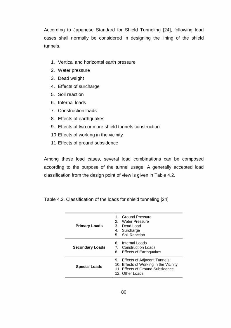
80

According to Japanese Standard for Shield Tunneling [24], following load

cases shall normally be considered in designing the lining of the shield

tunnels,

1. Vertical and horizontal earth pressure

2. Water pressure

3. Dead weight

4. Effects of surcharge

5. Soil reaction

6. Internal loads

7. Construction loads

8. Effects of earthquakes

9. Effects of two or more shield tunnels construction

10. Effects of working in the vicinity

11. Effects of ground subsidence

Among these load cases, several load combinations can be composed

according to the purpose of the tunnel usage. A generally accepted load

classification from the design point of view is given in Table 4.2.

Table 4.2. Classification of the loads for shield tunneling [24]

Primary Loads

1. Ground Pressure 2. Water Pressure 3. Dead Load 4. Surcharge 5. Soil Reaction

Secondary Loads 6. Internal Loads 7. Construction Loads 8. Effects of Earthquakes

Special Loads 9. Effects of Adjacent Tunnels 10. Effects of Working in the Vicinity 11. Effects of Ground Subsidence 12. Other Loads

81

Primary loads are the basic loads that should always be considered in the

design of linings. Secondary loads are the loads acting during construction or

after completion of the tunnel. These loads should be taken into account

according to the objective, the conditions of construction, and location of the

tunnel. On the other hand, the special loads are the loads specifically

considered according to the conditions of the ground and the tunnel usage.

The notations used for the structural calculation of lining are defined as

follows: bending moment (M), axial force (N), and shear force (Q) (for

member forces, the directions indicated in Figure 4.2 are assumed to be

positive).

Figure 4.2. Notations of bending moment, axial force, and shear force

4.2.1. Primary Loads

a) Earth Pressure: A section of tunnel and surrounding ground are shown in

Figure 4.3. The ground pressure should be calculated in accordance with

suitable analysis. For instance, the ground pressure should act radially on the

lining or be divided into the vertical ground pressure and the horizontal

ground pressure. Generally, the ground pressure is determined by dividing it

into horizontal and vertical components in order to simplify the calculations

[24].

82

Figure 4.3. Section of tunnel and surrounding ground [23]

i) Vertical Earth Pressure: The vertical ground pressure at the tunnel

crown should be a uniform load and should be equal to the overburden

pressure as a rule if the designed tunnel is a shallow tunnel. In other words, it

is preferable not to expect the effect of arch action at the soil for the tunnel of

which overburden (H) is less than the width of loosened soil (B). However, if

it is a deep tunnel, the effect of arch action occurs and reduced earth

pressure can be adopted in accordance with Terzaghi’s formula (4.2) and

Protodiaconov’s formula (4.3).

Soil

For shallow tunnels (H<B), ground pressure is equal to total overburden

pressure and can calculated in accordance with Equation 4.1. Regarding the

unit weight of soil for the calculation of earth pressure, the wet unit weight

should be used for soil above the ground water table and submerged unit

weight should be used for soil below the groundwater table.

∑ ∑++= iiiie HHPP γγ01 (4.1)

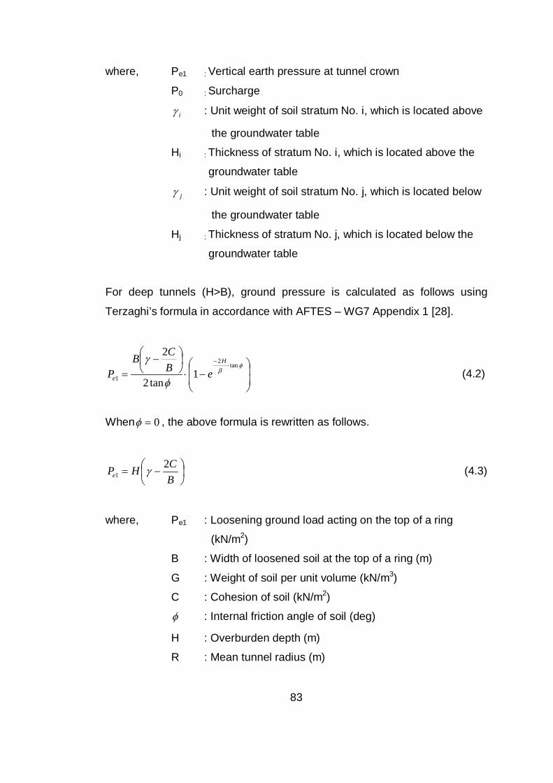
83

where, Pe1 : Vertical earth pressure at tunnel crown

P0 : Surcharge

iγ : Unit weight of soil stratum No. i, which is located above

the groundwater table

Hi : Thickness of stratum No. i, which is located above the

groundwater table

jγ : Unit weight of soil stratum No. j, which is located below

the groundwater table

Hj : Thickness of stratum No. j, which is located below the

groundwater table

For deep tunnels (H>B), ground pressure is calculated as follows using

Terzaghi’s formula in accordance with AFTES – WG7 Appendix 1 [28].

−⋅

−

=⋅

−φ

β

φ

γtan

2

1 1tan2

2H

e eBCB

P (4.2)

When 0=φ , the above formula is rewritten as follows.

−=

BCHPe

21 γ (4.3)

where, Pe1 : Loosening ground load acting on the top of a ring

(kN/m2)

B : Width of loosened soil at the top of a ring (m)

G : Weight of soil per unit volume (kN/m3)

C : Cohesion of soil (kN/m2)

φ : Internal friction angle of soil (deg)

H : Overburden depth (m)

R : Mean tunnel radius (m)

84

Figure 4.4. Calculation of loosening ground load

The width of loosened soil is calculated by the following equation.

−⋅=

483tan2 φπRB (4.4)

The minimum overburden thickness used to calculate the section force of a

segment is treated as follows:

H < B Whole Overburden

B < H < 2.5B Minimum Overburden B

H > 2.5B Minimum Overburden B

Rock

For tunnels to be bored in rock, the ground pressure is calculated by

Protodiakonov’s formula in accordance with AFTES-WG7 Appendix 1 [28].

σ ′=

10.01BPe (4.5)

where, B : Width of ground between slip planes, level with crown

σ ′ : Uniaxial compressive strength

85

ii) Horizontal Earth Pressure: The horizontal ground pressure should be

the uniformly varying load acting on the centroid of lining from the crown to

bottom. Its magnitude is determined as the vertical load pressure multiplied

by the coefficient of lateral earth pressure.

Soil

For tunnels to be bored in soil, the horizontal ground pressure is calculated

by the following equations, in accordance with AFTES-WG7 Appendix 1 [28].

ee Pq ⋅= λ (4.6)

φλ sin1−= (4.7)

where, qe : Horizontal ground pressure

Pe : Vertical ground pressure

λ : Coefficient of lateral ground pressure

φ : Internal friction angle of soil

Rock

The horizontal ground pressure acting on a tunnel section surrounded by

rock is calculated by the following equations, in accordance with AFTES-

WG7 Appendix 1 [28].

ee Pq ⋅= λ (4.8)

ννλ−

=1

(4.9)

where, qe : Horizontal ground pressure

Pe : Vertical ground pressure

λ : Coefficient of lateral ground pressure

ν : Poisson’s ratio

86

Vertical and horizontal ground pressures are illustrated in Figure 4.5.

Figure 4.5. Ground pressures acting on lining

b) Water Pressure: The water pressure acting on the lining should be the

hydrostatic pressure (see Figure 4.6). The resultant water pressure acting on

the lining is the buoyancy. The hydrostatic pressure in the ground is usually

calculated along the mean fiber of the lining in the radial direction. The

magnitude of water pressure is proportional to the depth measured from the

tunnel crown.

Figure 4.6. Hydrostatic pressure

87

)cos1(1 θγ −⋅+= cwww RPP (4.10)

www HP ⋅= γ1 (4.11)

where, Pw : Water pressure

Pw1 : Water pressure at tunnel crown

wγ : Unit weight of water

Rc : Radius of a circle of the centroidal line of segments

θ : Angle from tunnel crown (clockwise)

Hw : Depth of water at tunnel crown

c) Dead Load: The dead weight of the segments per unit length is calculated

as a vertical load distributed along the centroid of the lining. It is calculated in

accordance with Equation 4.9.

cRWg⋅

=π2

11 (4.12)

where, 1g : Dead weight of the segments per unit length

1W : Weight of one ring of segments

cR : Radius of a circle of the centroidal line of segments

d) Surcharge: The effect of surcharge acting on the tunnel is determined by

taking into consideration the distribution of the stress in the ground. It

increases earth pressure acting on the lining. The following loads are

considered as surcharge in design:

• Road traffic load

• Railway traffic load

• Weight of buildings

• All future expected loads

88

e) Soil Reaction: Among all the loads acting on the lining, soil reaction is the

generic name of the design ground reaction, which is distinguished from the

imposed loads determined independently. Considerations on soil reactions

are different depending on the design calculation method employed [24].

In the usual calculation method, the vertical soil reaction caused by the

imposed loads is irrelevant to the ground deformation and it is the uniform

reaction equilibrating to these imposed loads. On the other hand, horizontal

soil reaction acting on the tunnel can be defined as the generated reaction by

the displacement of the lining towards the ground and it has a triangular

distribution with the peak intensity at the spring line spreading within the

range of the central angle of ± 45° from the spring line.

Contrary to usual calculation method, soil reaction is the uniform reaction

balancing the vertical ground pressure at the bottom of the tunnel in BSMs.

Especially, in case of large diameter tunnels, the dead weight of segments

can be taken into consideration in BSMs.

4.2.2. Secondary Loads

a) Internal Loads: The internal load is a load which acts inside the lining

after completing the tunnel and is determined according to the actual

condition. The railway vehicle load acting on the bottom of the lining is

considered as internal load. In addition, internal water pressure should be

taken into consideration in conveyance tunnels as an internal load [23].

b) Construction Loads: The design of segments takes into consideration

the construction conditions and following loads [24].

i) Thrust Force of Jacks: The thrust force of jacks is a temporary load

that is applied to the segment rings when advancing the shield machine. It is

89

the most influential force among the loads acting on the segments during

construction.

ii) Backfill Grouting Pressure: Where backfill grout is injected in a well-

controlled manner, the exterior surface of the segment ring is subjected to a

force similar to fluid pressure. The backfill grout pressure acting on the

segments varies depending on the grouting method and the grout conditions.

In actual construction, the segments can be subjected to locally large

pressures. Therefore, it is necessary to consider these pressures in the

design. In normal cases, it is acceptable to use the value 100 kN/m2 for

grouting pressure.

iii) Load from Erector Operation: The load from erector operation is one

of the loads acting on the segments. The load from erector operation is taken

into account when designing the segment hangers and when evaluating the

effect of load on the segments during their erection.

iv) Superimposing: The superimposing load is the other one under the

condition where segments are superimposed during their storage and

transportation. The impact during storage and transportation is taken into

consideration by multiplying the load by the impact coefficient.

v) Other Loads: In addition to loads mentioned above, other construction

loads such as dead weight of the trailing gear, jack load of the tunnel shape

retainer, the cutter rotation force, and the loads being determined by the

shield type, etc. are considered if needed.

c) Effects of Earthquakes: If the tunnel is driven through relatively uniform

soils and has a large overburden, the effects of earthquakes are considered

to be small since the tunnel behaves in a way similar to that of the

surrounding soils. However, if the tunnel is subjected to any of the following

90

conditions, it could be greatly affected by the behavior of the surrounding

soils, and the effects of earthquakes are determined by consideraing the

dynamic interaction between the tunnels and surrounding soil [24]:

• When the lining structure changes suddenly.

• When the tunnel is in soft ground.

• When the ground conditions such as geology, overburden and

bedrock depth change suddenly.

• When the alignment includes sharp curves.

• When the tunnel is in loose saturated sand and there is a possibility

of liquefaction.

4.2.3. Special Loads

a) Effects of Adjacent Tunnels: Where two or more tunnels are constructed

near each other, the preceding tunnel could be affected by the succeeding

tunnel and their interaction creates earth pressures and soil reactions

different from those cases where only one tunnel is driven. Moreover, such

an interaction could cause long-term adverse effects on the tunnels.

Where two tunnels are driven near each other, the succeeding tunnel is

bored through soils supporting the soil mass above the proceeding tunnel.

This redistributes the stresses in the ground and increases the vertical

pressure acting on the preceding tunnel. The vertical pressure acting on the

succeeding tunnel is smaller than that acting on the preceding tunnel and

differs from the vertical pressure acting on a single tunnel when no other

tunnel is near by.

It is necessary to perform analyses by properly modeling the ground

conditions and by taking into consideration such factors as the relative

location of the tunnels, and their outer diameters and conditions during

91

construction in order to develop a design method that can perfectly solve this

type of problems [24].

b) Effects of Working in the Vicinity: When it is anticipated that other

structures are to be constructed in close proximity during or after a shield

tunneling, an assessment should be made if any bad effect may exert.

If any of the following four conditions exists, there should be made an

appropriate evaluation of loads with considering a rational calculation

method. Moreover, when evaluating a secondary lining as a structural

member for future load fluctuation, an appropriate model for structural

calculation should be cosidered [24].

• When a new structure is constructed directly above or is excavated

resulting in a great change in the surcharge.

• When the soil directly above or below a tunnel is excavated resulting

in a great change in the condition of vertical or horizontal earth

pressure and ground characteristics such as the coefficient of soil

reaction.

• When the ground at the side of the tunnel is disturbed resulting in a

great change in the lateral or resistance earth pressure.

• When there is a great change in the water pressure working on the

tunnel.

c) Effects of Ground Subsidence: When constructing a tunnel in soft

ground, attention should be paid to how the soil characteristics affect ground

settlement apart from those caused by the tunnel construction process. It is

necessary to consider the effects of ground settlement on the tunnel and the

joints between the tunnel and the shaft. The effects of ground settlement on

the tunnel can be studied in two ways:

92

• Study of the effect of consolidation settlement on the tunnel in the

transverse direction.

• Study of the effect of unequal settlement on the tunnel in the

longitudinal direction.

Moreover, relative displacement tends to occur at the joint between the

tunnel and the shafts because different types of structures are connected at

these positions. Therefore, it is desirable to prevent stress concentrations by

applying the flexible joints where necessary or to reduce the effect of relative

settlement by making the foundation of the shaft a floating foundation [24].

d) Other Loads: Apart from abovementioned special loads, specific cases

such as fire, explosion, train derailment, and temperature changes, etc. can

be considered depending on the conditions of the tunnel project.

4.3. Structural Calculation Procedure In order to perform structural calculations for design, the first four steps of

design procedure given in Chapter 4.1.3 should be implemented. In other

words, specifications and codes to be used, inner dimensions of tunnel, load

and lining conditions should be decided before this stage.

4.3.1. Critical Sections After determining the lining and loading conditions, the design calculation of

the tunnel cross-section should be done for the following critical sections.

• Section with deepest and shallowest overburden

• Section with highest and lowest ground water table

• Section in the case of rapid change in the ground

• Section with large surcharge

• Section with eccentric loads

93

• Section with unlevel surface

• Section with adjacent tunnel at present or to be done in future

4.3.2. Computation of Member Forces For the design of segmental lining sections, member forces (M, N, S) can be

calculated by using several structural models. Structural analysis methods

used to determine member forces are determined in Chapter 3 in detail. All of

these methods have strengths and weaknesses. For that reason, proper

analysis method may change depending on the conditions of the project.

Among the structural analysis methods expressed in Chapter 2, beam-spring

method that simulates the interaction between the lining and surrounding

ground realistically is the most widely used method due to its effectiveness.

In spite of being a simple and limited method type, analytical methods, i.e.

elastic equation method, are also utilized in order to compare and evaluate

the results obtained by more sophisticated methods. Accordingly, the

evaluation of elastic equation method and beam-spring methods is

implemented in Chapter 5.

4.3.3. Safety of Section After the calculation of member forces with a selected analysis method, the

safety of critical sections should be checked using the limit state design

method or the allowable stress design method. Sections to be checked are

as follows [23]:

• Section with maximum moment

• Section with maximum axial force

• Section with maximum shear force

94

4.3.4. Limit State Design Method The interaction diagram as shown in Figure 4.7 describes the relationship

between the design axial capacity and the design flexural capacity of

member cross-sections subjected to axial load and flexural moment. If the

point (Md, Nd) is located inside the (Mud, N’ud) curve at the side of the origin,

the section is safe against the design loads according to limit state design

method.

Figure 4.7. Interaction diagram [23]

4.3.5. Allowable Stress Design Method If the extreme fiber stress of concrete and the stress of reinforcement are

less than their allowable stresses, the section is safe against the design

loads according to allowable stress design method (see (4.13) and (4.14)).

cckcac Ff /=≤ σσ (4.13)

sydsas Ff /=≤ σσ (4.14)

95

where, cσ : Extreme fiber stress of concrete

caσ : Allowable stress of concrete

ckf : Characteristic compressive strength of concrete

cF : Safety factor of concrete

sσ : Stress of reinforcement

saσ : Allowable stress of steel

ydf : Yield stress of steel

sF : Safety factor of steel

4.3.6. Safety of Joints The flexural rigidity of segmental lining at the joint is smaller than the flexural

rigidity of the segment. Also, if the segments are staggered, the moment at

the joint is smaller than the moment of the adjacent segment. The actual

effect of the joint should be evaluated in the design. Accordingly, the safety of

joints can be checked by the same method with sections as determined in

Chapter 4.3.3 by considering the effect mentioned above.

96

CHAPTER 5

METHODS OF ANALYSES

There are several analysis methods recommended for the design of TBM

segmental linings as described in Chapter 3. Each method has its typical

assumptions and approaches differently. For that reason, it is necessary to

compare these methods for certain situations in order to determine the

efficiencies of each method. In this chapter, selected analytical and numerical

methods are implemented for a typical railway tunnel, and the sensitivities of

methods are compared under certain situations.

For the evaluation, elastic equation method and Beam – Spring Method are

carried out as analytical and numerical methods, respectively. As described

in Chapter 3, elastic equation method based on simple assumptions is a

practical way for the analysis of circular tunnels. Besides, Beam – Spring

Method is the most widely used numerical method that is able to simulate the

structural behavior of segmental rings. Also, there exist many different

approaches for 2D and 3D BSMs. In this chapter, various structural models

including elastic equation method, 2D and 3D BSMs with different

approaches are employed for a rational comparison.

Literature review of TBM segmental lining analysis methods provided along

with recent published studies shows that 3D BSM gives reasonable results

compatible with finite element models, laboratory tests, and on-site

measurements. This study investigates the sensitivity of elastic equation

method and 2D BSMs by comparing 3D BSM. As a result of this comparison,

97

the applicability of methods is introduced. Also, the effects of mesh

coarseness, shear stiffness between the ring connections, arrangement of

key segments, rapid change in surcharge, and sharp alteration in soil

stiffness are investigated and the competence of 2D and 3D models for these

effects is indicated. The situations described above are examined in terms of

the changes in the forces, moments, and deflections of the lining.

A multipurpose structural analysis and design software, “LARSA 4D”, has

been utilized in order to carry out beam – spring analyses. Structural

applications require advanced models for the simulation of the non-linear,

time-dependent, and inelastic behavior of structural elements. The LARSA

4D is equipped with special features to deal with the numerous aspects of

complex structural elements. Moreover, it has functional modeling tools

including meshing, generation, templates, and advanced drawing and it is

especially suitable for BSM analyses, because it has specific elements such

as non-tension ground springs for ground – tunnel interaction, two-node

spring elements for ring joints, one-node rotational spring elements for

segment joints, member end releases for simulating segments connected

with hinges, and etc.

5.1. The Geometry of the Problem The tunnel cross-section and geometry of the problem are given in Figure 5.1

and Figure 5.2, respectively. As it is shown in Figure 5.1, the typical TBM

segmental ring having a circular shape consists of four ordinary segments

(A1, A2, A3, and A4), two counter segments (B1 and B2), and one key

segment (K1). Key segment is located at 43.2° from the crown and has a

degree of 14.4º which is the quadrant of the other segments. The thickness

and width of the linings are estimated as 320 mm and 1500 mm respectively

according to the ranges summarized in Table 2.2. The outer and inner

diameters of the ring are 7680 mm and 7040 mm, respectively. Also, 25 cam-

and-pocket type ring joints regularly located are shown in the Figure 5.1.

98

Figure 5.1. Tunnel cross-section

General properties of ring used in the analyses are summarized as follows:

Type of tunnel : TBM Tunnel

Type of segment : Reinforced concrete segment

Type of segment joint : Flat type joints

Type of ring joint : Cam-and-pocket

Outer diameter of ring : 7680 mm

99

Inner diameter of ring : 7040 mm

Width of segment : 1500 mm

Thickness of segment : 320 mm

Partitions : 4 ordinary + 2 counter + K segment

Type of key segment : Axially inserted type

The excavation and loading geometries of the problem are in a range which

is common in civil engineering practice. The cover depth of the tunnel is

15402 mm as shown in Figure 5.2. Also, the groundwater level is situated

5994 mm above the tunnel crown.

Figure 5.2. Geometry of the problem (not to scale)

100

5.2. Geotechnical and Material Parameters The tunnel is surrounded by relatively hard clay. Also, earth fill, hard clay,

and dense sandy soil layers exist above the tunnel. Geotechnical properties

of these layers are given in Table 5.1.

Table 5.1. Geotechnical parameters of the soil layers

Parameters Earth Fill Hard Clay Dense Sandy Soil

Average SPT N Value 8 29 33

Saturated Unit Weight (kN/m3)

19 19 20

Internal Friction Angle (°)

27 - 40

Cohesion (kN/m2)

- 170 -

Poisson’s Ratio 0.35 0.40 0.40

Modulus of Elasticity (kN/m2)

22400 81200 92400

Mechanical properties of precast reinforced concrete segments and steel

reinforcement bars used as supporting elements are listed below:

Compressive strength of concrete: fck = 50 N/mm2

Tensile strength of concrete: fct = 4.1 N/mm2

Modulus of elasticity of concrete: Ec = 37 kN/mm2

Poisson’s ratio of concrete: = 0.20

Unit weight of concrete: c = 26 kN/m3

Yield strength of steel reinforcement bars: fy = 420 N/mm2

Modulus of elasticity of steel: Es = 200 kN/mm2

101

5.3. Analytical Analysis with Elastic Equation Method As an analytical approach, elastic equation method is used to analyze the

segmental lining in this study. As discussed in Chapter 3, this method is a

practical and most widely used analytical tool for the analysis of segmental

linings. Due to its limitations mentioned in Section 3.1.1, this method is not

used for the final design calculations, but it might be quiet useful to get a first

idea of the forces in the lining.

In order to calculate member forces with this method, working sheets are

developed by using Microsoft Excel 2003 and Macro Visual Basic

applications. Input sheet, load condition sheets, and member forces sheet

are given in Appendix A (Figure A1-A4). Input sheet includes geometrical,

material, and geotechnical properties of the problem. Calculations of loads

and member forces are also provided in load conditions sheet and member

forces sheet, respectively.

For the vertical earth pressure, the depth of tunnel is not adequate for

arching action. Therefore, total overburden governs the vertical earth

pressure. Calculations performed for other loads are also given in the

Appendix A.

Member forces for any location on the ring can be obtained by this method.

The sheet is generated to obtain the most critical member forces occurred on

the ring. However, calculations to obtain member forces are performed for a

segmental ring with unit width. Therefore, the results of this analysis are

multiplied by 1.5 in order to obtain member forces for the segmental ring with

a width of 1.5 m.

The evaluation and comparison of results obtained by elastic equation

method and 2D and 3D Beam – Spring Methods are mentioned in the next

chapter.

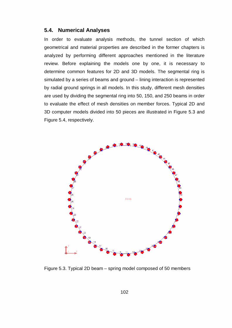
102

5.4. Numerical Analyses In order to evaluate analysis methods, the tunnel section of which

geometrical and material properties are described in the former chapters is

analyzed by performing different approaches mentioned in the literature

review. Before explaining the models one by one, it is necessary to

determine common features for 2D and 3D models. The segmental ring is

simulated by a series of beams and ground – lining interaction is represented

by radial ground springs in all models. In this study, different mesh densities

are used by dividing the segmental ring into 50, 150, and 250 beams in order

to evaluate the effect of mesh densities on member forces. Typical 2D and

3D computer models divided into 50 pieces are illustrated in Figure 5.3 and

Figure 5.4, respectively.

Figure 5.3. Typical 2D beam – spring model composed of 50 members

103

Figure 5.4. Typical 3D beam – spring model composed of 50 members

The ground-lining interaction is modeled as linear elastic springs of which

constants are calculated by the equation proposed by Muir Wood, in

accordance with AFTES – WG7 Appendix 1 [28]. It is assumed that ground

reaction forces are activated when the tunnel expands outward, but they are

not activated when the tunnel contracts inward. Therefore, non-tension

(compression only) springs are used in the analysis. The graph showing the

constants of non-tension ground springs for 3 different mesh densities is

given in Figure 5.5. As shown in figure, ground springs are assumed to have

a linear elastic behavior. Ground spring constants are obtained by multiplying

coefficient of subgrade reaction with the tributary area of springs.

104

Ground springs are placed at each member joint in radial direction and so the

number of ground springs is equal to the number of beam members. The

ground behavior in tangential direction is generally ignored in BSMs.

Although this leads to frictionless sliding of the lining against the ground, it

has a negligible effect on member forces. For that reason, ground springs are

only considered in radial direction.

Figure 5.5. Ground spring constants

Contrary to elastic equation method, there is no need to multiply the results

of computer models, because the calculations of computer models are done

for a ring with a width of 1.5 m. Therefore, the cross-sectional area of lining

(A) and moment of inertia of lining (I) per ring are calculated as follows:

)32.0,5.1(48.032.05.1 2 mthicknessmwidthsegmentmA ===×=

433 10096.432.05.1121 mI −⋅=××=

Abovementioned features of sections to be analyzed constitute the input

parameters of computer models. These input parameters of models with

different mesh densities are listed in Table 5.2.

105

Table 5.2. General features of beam - spring models

Features Model with 50 beams

Model with 150 beams

Model with 250 beams

# of Members 50 150 250

# of Ground Springs 50 150 250

# of Nodes 100 300 500

Length of Members (lb) 462mm 154mm 92.5mm

Radius of Ring (Rc) 3,680mm 3,680mm 3,680mm

Width of Segments (w) 1,500mm 1,500mm 1,500mm

Thickness of Segments (t) 320mm 320mm 320mm

Moment of Inertia of Segments (I)

4.096 E-03m4 4.096 E-03m4 4.096 E-03m4

Cross-sectional Area of Segments (A)

0.48m2 0.48m2 0.48m2

Modulus of Elasticity (E) 81,200kN/m2 81,200kN/m2 81,200kN/m2

Coefficient of Lateral Earth Pressure

=

−= 4.0,

1ν

ννλ

0.67 0.67 0.67

Coefficient of Subgrade Reaction

( ) )1

(cR

Ek⋅+

=ν

15,760kN/m3 15,760kN/m3 15,760kN/m3

Ground Spring Constant

( )wlkk br ⋅⋅= 10,925kN/m 3,643kN/m 2,187kN/m

106

5.4.1. 2D Structural Models Theoretical approaches on BSMs have been discussed in Chapter 3. The

important point in beam – spring method is the modeling of connections.

Since 2D models are unable to simulate the ring joints, the difference

between these 2D models is the modeling of segment joints. In this study, all

2D approaches mentioned in Chapter 3 are performed by computer models.

Totally, four different 2D approaches are analyzed and evaluated and the

descriptions of these models can be summarized as follows.

a) Model A (Rigid Ring): This is the simplest 2D model that assumes the

ring having a uniform bending stiffness (EI). In other words, segment joints

are assumed to be fully rigid connections. Due to this assumption, reduction

of rigidity at the segment joints is ignored. In this model, the stiffness

parameters (E and I) of segment section are also used for segment joints in

order to obtain fully rigid ring.

b) Model B (Muir Wood): This model also assumes the ring having a

uniform bending stiffness. However, a reduced bending stiffness is used in

order to simulate the effect of segment joints. The reduction in the bending

stiffness can be calculated according to several approaches mentioned in

Chapter 3. In this study, the approach proposed by Muir Wood [27] is utilized.

The effective moment of inertia can be calculated by using the following

formula (Formula 3.3) which depends on the section at the force transmission

zone and number of segments.

4332

32

10332.210096.464160,05,1

1214 mI

nII jeff

−− ⋅=⋅⋅

+⋅⋅=⋅

+=

The stiffness of the lining section is reduced by using this effective moment of

inertia for the entire section. Since the structure in this model is more flexible,

107

it gives lower sectional forces and bending moments. Therefore, this

approach leads to more economical results for the design.

c) Model C (Multiple Hinges): In this model, segment joints are modeled as

unfixed hinges. Figure 5.6 illustrates the configuration of segment joints at

which the hinges are located. Not only the number of segment joints, but also

the segment orientation is considered by means of these hinges. However, a

ring with multiple hinged joints is an unstable structure. Therefore, the model

may encounter convergence problems. In order to prevent convergence

problems, 90 % of bending moments at segment joints is released and 10 %

of moments occurred at the segment joints is kept. Normally, uniform

bending stiffness is used in this method.

Figure 5.6. Configuration of segment joints in 2D models

d) Model D (Rotational Springs): This model simulates the segment joints

as rotational springs. This enables the model to consider both the number

and orientation of segments. The configuration of segment joints at which the

rotational springs are located is shown in Figure 5.6. Linear and non-linear

approaches are available for rotational spring constants. If only a linear

rotational spring with the definition of a yielding moment is performed, the

simulation of behavior of the joints seems to be too rough. In order to have

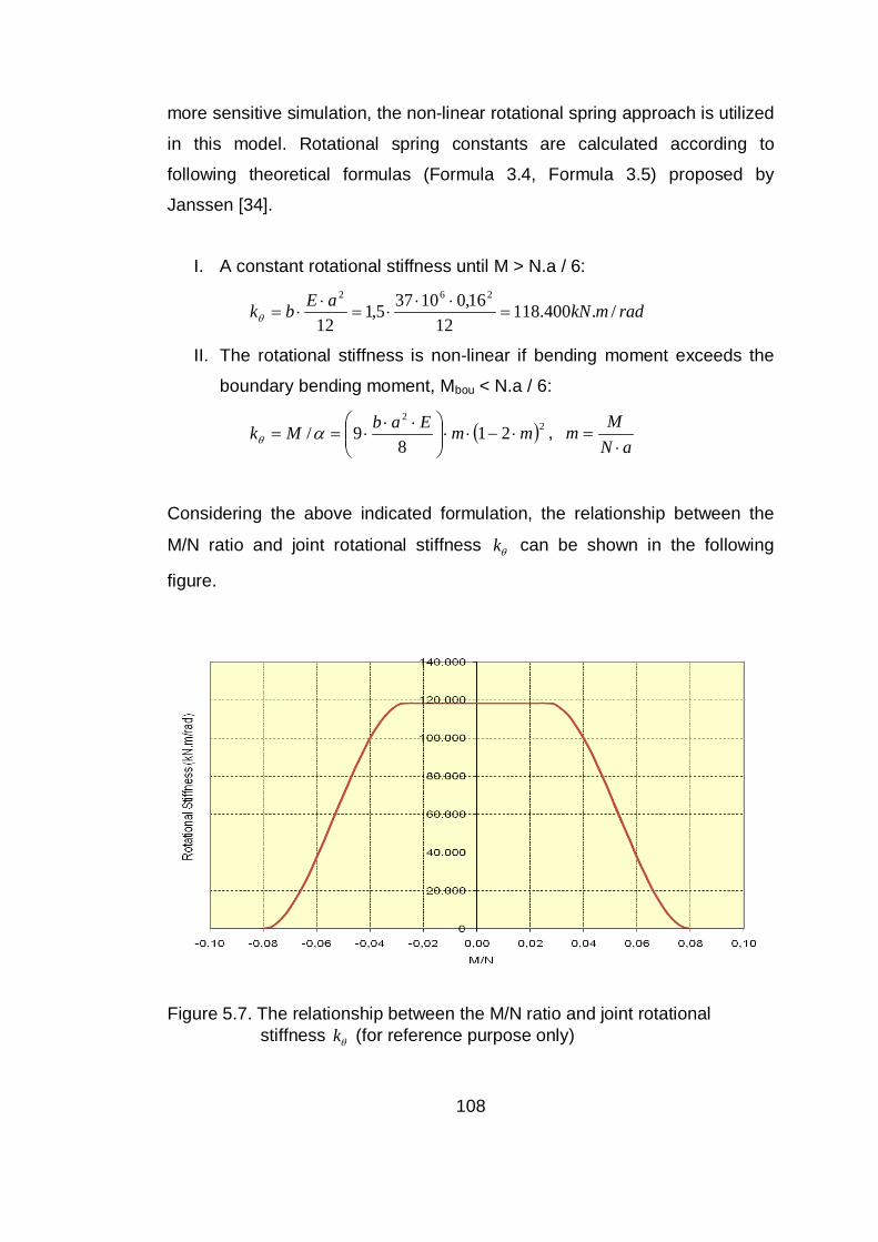
108

more sensitive simulation, the non-linear rotational spring approach is utilized

in this model. Rotational spring constants are calculated according to

following theoretical formulas (Formula 3.4, Formula 3.5) proposed by

Janssen [34].

I. A constant rotational stiffness until M > N.a / 6:

radmkNaEbk /.400.11812

16,010375,112

262

=⋅⋅

⋅=⋅

⋅=θ

II. The rotational stiffness is non-linear if bending moment exceeds the

boundary bending moment, Mbou < N.a / 6:

( )22

218

9/ mmEabMk ⋅−⋅⋅

⋅⋅⋅== αθ ,

aNMm⋅

=

Considering the above indicated formulation, the relationship between the

M/N ratio and joint rotational stiffness θk can be shown in the following

figure.

Figure 5.7. The relationship between the M/N ratio and joint rotational

stiffness θk (for reference purpose only)

109

Janssen formulation allows taking into account the decrease in rotational joint

stiffness due to the joint rotation. In order to do this, an iterative procedure

has been carried out on the basis of the results of Larsa4D computation.

Several iterations have been carried out to match the actual joint rotational

stiffness (rigidity) which is the input parameter of the Larsa4D program with

the M/N ratio calculated from formulation Different joint stiffness and behavior

have been considered depending from the applied moment, and axial force

for each rotational spring.

In detail, each iteration has been carried out as follows:

- A tentative joint rotational rigidity (118.400 kN.m/rad) has been taken

as input value in BSMs for each joint.

- The numerical model has been run and the maximum M/N value

computed at the joints has been plotted on the chart given in Figure

5.7.

If the value corresponding to the input rigidity and the resulting M/N ratio

does not correspond to a valid point on the Janssen curve, the steps

indicated above are repeated. After the first iteration, bending moment and

axial force acting on the joints are used as an input for Janssen computation

and a new rotational stiffness is calculated for each joint. This procedure is

performed until the match is found.

The example of iteration process carried out to match the input rigidity with

the output M/N ratio is given in Figure 5.8. Red dots indicate the results of

last (nth) iteration that fully match with the Janssen curve. As shown from

figure, some of green dots that indicate the (n-1)th iteration results do not fit

on the Janssen curve and one more iteration is needed. Figure 5.8 also

shows the range –a/6 < M/N < a/6 where rotational stiffness is constant. As

110

the absolute value of M/N out of this range increases, the rotational stiffness

of the joint decreases and this leads to increase in rotational deformation.

Figure 5.8. The iteration process for the computation of joint rotational stiffness

Iteration processes of all rotational springs used in 2D and 3D BSMs are

enclosed in Appendix B.

5.4.2. 3D Structural Model 3D BSMs are able to simulate the segment and ring joints for sequential

rings. In this study, 3D BSM proposed by Koyama [38] is performed. Model

VI described in Section 3.2 is used as a reference in order to constitute the

3D model.

111

The configuration of 3D BSM for three adjacent rings is shown in Figure 5.4.

It consists of several beams forming the segments, rotational springs

between the segment joints, shear springs between the adjacent rings, and

ground springs representing the ground – lining interaction. The modeling of

rotational and ground springs is the same with 2D models. Therefore, Figure

5.5 and Figure 5.7 that show the ground and rotational spring constants

respectively are also valid for this model.

The major difference of this 3D model from 2D models is the shear springs at

ring joints that enable 3D models to simulate interaction between adjacent

rings. Furthermore, 3D models are able to represent the staggered geometry

of sequential rings. In order to represent the staggered geometry, three

sequential rings are modeled and connected to each other by shear springs.

The configuration and staggered geometry of segment joints are illustrated in

Figure 5.9.

Figure 5.9. Configuration of segment joints in 3D models

The shear springs are located at each ring joint which is distributed around

the ring uniformly. The configuration of 25 ring joints can be seen in Figure

5.1. As discussed in Section 3.2, the calculation for a shear spring constant is

112

a complex issue, and there is no general formula available in the literature for

determining the shear spring constant. In this study, the shear spring

constant is assumed to be 20.000 kN/m in radial direction. This is a

reasonable value for a segmental ring with segment thickness of 320 mm

and shear strip width of 50 mm. Since a shear strip is placed on both end of

each segment, the shear spring constant between two adjacent rings is

calculated as follows:

mkNks /000.402000.20 =×=

The shear spring constant is selected by considering comparable studies

performed by BSMs. The graph showing the shear spring constant used in

3D models is given in Figure 5.10.

40000

-40000-60000

-40000

-20000

0

20000

40000

60000

-1,5 -1 -0,5 0 0,5 1 1,5

Displacement (m)

Shea

r For

ce (k

N)

Figure 5.10. Shear spring constant

5.5. Loading Conditions Loading conditions for a tunnel differ from others depending on soil profile,

soil and material properties, longitudinal profile of the route, geometry, type

and usage area of tunnel, and etc. In this study, primary load cases are

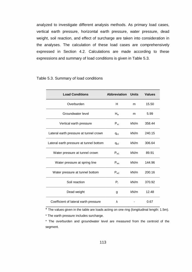
113

analyzed to investigate different analysis methods. As primary load cases,

vertical earth pressure, horizontal earth pressure, water pressure, dead

weight, soil reaction, and effect of surcharge are taken into consideration in

the analyses. The calculation of these load cases are comprehensively

expressed in Section 4.2. Calculations are made according to these

expressions and summary of load conditions is given in Table 5.3.

Table 5.3. Summary of load conditions

Load Conditions Abbreviation Units Values

Overburden H m 15.50

Groundwater level Hw m 5.99

Vertical earth pressure Pvc kN/m 358.44

Lateral earth pressure at tunnel crown qe1 kN/m 240.15

Lateral earth pressure at tunnel bottom qe2 kN/m 306.64

Water pressure at tunnel crown Pw1 kN/m 89.91

Water pressure at spring line Pws kN/m 144.96

Water pressure at tunnel bottom Pw2 kN/m 200.16

Soil reaction Pr kN/m 370.92

Dead weight g kN/m 12.48

Coefficient of lateral earth pressure λ - 0.67

* The values given in the table are loads acting on one ring (longitudinal length: 1.5m).

* The earth pressure includes surcharge.

* The overburden and groundwater level are measured from the centroid of the

segment.

114

Load combination used in the analyses is selected by considering

serviceability limit state (SLS). Basic load combination for SLS proposed by

AFTES [43] is given in Table 5.4.

Table 5.4. Combination of loads

Loads Basic Load

Combination (SLS)

Vertical Ground Load 1.0

Horizontal Ground Load 1.0

Hydrostatic Loads 1.0

Dead Load 1.0

Surcharge 1.0

Soil Reaction 1.0

5.6. Flowchart of Calculation Analysis of TBM segmental linings is investigated both with analytical and

numerical methods. Also, variations in input parameters and conditions of the

problem are examined in order to evaluate 2D and 3D BSMs.

The studies carried out for the given tunnel cross-section can be summarized

as follows:

CASE 1: The analyses of given tunnel section are performed by using

analytical (elastic equation method) and numerical (2D and 3D BSMs)

methods of which definitions are previously given. The comparison of

115

analysis methods is carried out by evaluating the results of models

performed.

Firstly, 2D analytical and numerical methods are compared between each

other. Then, results obtained from 2D analytical and numerical methods are

compared together with 3D BSM. By means of this comparison; the

sensitivities of analysis methods are assessed.

CASE 2: Comparison of 2D and 3D BSMs is also carried out for the tunnels

passing through a transition zone having relatively different soil stiffness.

Tunnel with a length of 9 m is modeled by 6 sequential rings. It is assumed

that there is a sharp transition from stiff soil to soft soil in the middle of the

model. Soil profile of the tunnel route is given in Figure 5.11.

Figure 5.11. Soil profile of the tunnel route

Three different transition zones having different soil stiffness are selected for

the evaluation. The moduli of elasticity of stiff and soft soils in these transition

zones to be analyzed are given in Table 5.5. Difference in soil stiffness is

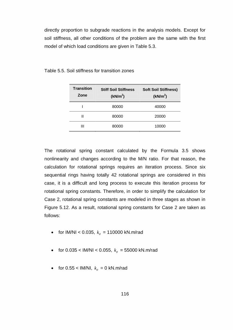
116

directly proportion to subgrade reactions in the analysis models. Except for

soil stiffness, all other conditions of the problem are the same with the first

model of which load conditions are given in Table 5.3.

Table 5.5. Soil stiffness for transition zones

Transition Zone

Stiff Soil Stiffness (kN/m2)

Soft Soil Stiffness) (kN/m2)

I 80000 40000

II 80000 20000

III 80000 10000

The rotational spring constant calculated by the Formula 3.5 shows

nonlinearity and changes according to the M/N ratio. For that reason, the

calculation for rotational springs requires an iteration process. Since six

sequential rings having totally 42 rotational springs are considered in this

case, it is a difficult and long process to execute this iteration process for

rotational spring constants. Therefore, in order to simplify the calculation for

Case 2, rotational spring constants are modeled in three stages as shown in

Figure 5.12. As a result, rotational spring constants for Case 2 are taken as

follows:

• for IM/NI < 0.035, θk = 110000 kN.m/rad

• for 0.035 < IM/NI < 0.055, θk = 55000 kN.m/rad

• for 0.55 < IM/NI, θk = 0 kN.m/rad

117

0

20,000

40,000

60,000

80,000

100,000

120,000

140,000

-0.08 -0.06 -0.04 -0.02 0.00 0.02 0.04 0.06 0.08M/N

Rig

idity

(kN

m/r

ad)

Theoretical ModelComputational Model

Figure 5.12. Theoretical and computational models of the rotational spring

constant

The calculation is made with 2D BSMs for the tunnel section both in stiff and

soft soil individually. The calculation is also performed by 3D BSM for the

entire profile and the results of 2D and 3D models are compared for the

evaluation.

CASE 3: A shallow tunnel passing under an existing structure is also

analyzed in order to compare 2D and 3D BSMs simulating the effect of

sudden change in loading conditions. A surcharge pressure of 100 kN/m2 is

assumed to occur along 9 m in the longitudinal direction. The Figure 5.13

shows the longitudinal profile of tunnel under surcharge pressure.

118

Existing surcharge pressure of 100 kN/m2 on the ground is distributed to

tunnel lining with a slope of 1H:2V. Equivalent surcharge pressure acting on

the tunnel lining is calculated as 60 kN/m2 along 15 m in the longitudinal

direction. Therefore, the surcharge load is taken as 90 kN/m for a ring with

length of 1.5 m.

Figure 5.13. Longitudinal profile of the tunnel under surcharge pressure

The tunnel is modeled for 30 m length and composed of 21 sequential rings.

The first 15 m of the tunnel is not exposed to surcharge load, although the

rest is under the surcharge load. The tunnel is assumed to be surrounded by

hard clay of which geotechnical properties are given in Table 5.1. In addition,

the loads acting on the lining are calculated as expressed in Section 4.2. The

summary of loads for this model is given in Table 5.6.

119

21 sequential rings having totally 147 rotational springs are examined for this

case. Therefore, it is also a difficult and long process to execute iteration

process for rotational spring constants. For that reason, in order to simplify

the calculation for Case 3, rotational spring constants are also modeled in

three stages as shown in Figure 5.12.

Table 5.6. Summary of load conditions for Case 3

Load Conditions Abbreviation Units Values

Vertical earth pressure Pvc kN/m 111.00

Lateral earth pressure at tunnel crown qe1 kN/m 74.00

Lateral earth pressure at tunnel bottom qe2 kN/m 93.37

Water pressure at tunnel crown Pw1 kN/m 40.00

Water pressure at spring line Pws kN/m 76.70

Water pressure at tunnel bottom Pw2 kN/m 113.40

Surcharge pressure on the lining Ps kN/m 90.0

Soil reaction Pr kN/m 123.48

Dead weight g kN/m 12.48

Coefficient of lateral earth pressure λ - 0.67

The calculation is made with 2D BSMs for tunnel sections in and out of

surcharge impact area. Also, 3D BSM is performed for the entire region and

the results of 2D and 3D analyses are compared. By this way, the necessity

of 3D models for the analysis of tunnels under the surcharge effect is

checked.

120

CASE 4: Selecting a proper mesh density is an important subject in

numerical analyses. For that reason, in order to evaluate the effect of mesh

coarseness in 2D and 3D BSMs, the analyses are performed by dividing the

segmental ring into 50, 150, and 250 beam elements. Then, sectional forces

and crown deformation obtained from 2D and 3D BSMs having different

mesh densities are compared.

CASE 5: In addition to mesh coarseness, another variable in 3D Beam –

Spring Method is the shear spring constant. For the ring section examined in

this study, the shear spring constant is selected as an average value of

20000 kN/m by considering previous studies. As mentioned in Section 3.2,

the shear spring constant varies by material used in ring joints and its

properties, such as shear modulus, area, and thickness. For that reason, in

order to evaluate the effect of shear spring constant in 3D Beam – Spring

Method, three different analysis models having a shear spring constant of

15000 kN/m, 20000 kN/m, and 25000 kN/m are examined, respectively.

Consequently, the sensitivity of shear spring constant is determined by

comparing the obtained results.

CASE 6: As a whole, key segments are placed in a staggered layout typically

having an equal angle about the vertical axis. In this sense, the arrangement

of key segments can be determined in various positions. In order to

investigate the effect of segment layout on the results obtained from 3D

Beam – Spring Method, four different segment arrangements are

implemented as shown in Figure 5.14. Rings having these different key

segment arrangements are analyzed with 3D BSMs and the results of

models are compared for the evaluation.

121

Figure 5.14. Segment configurations for 4 different layouts

122

The summary of abovementioned analysis cases is given in Table 5.7.

Table 5.7. Summary of analysis cases

Analysis Cases Analysis Cases

Case 1 Case 2 Case 3 Case 4 Case 5 Case 6

Method of Calculation

EEM

2D BSM

3D BSM

2D BSM

3D BSM

2D BSM

3D BSM

2D BSM

3D BSM 3D BSM 3D BSM

Reduced Bending

Stiffness (EI)eff

Only

Model B X X

Only

Model B X X

Simulation of Segment Joint

Model C

Model D

3D BSM

√ √ Model C

Model D

3D BSM √ √

Simulation of Ring Joint

Only

3D BSM

Only

3D BSM

Only

3D BSM

Only

3D BSM √ √

Type of Soil Stiff Soil Stiff Soil

Soft Soil Stiff Soil Stiff Soil Stiff Soil Stiff Soil

Mesh Coarseness

(ring divided by) 50 50 50

50

150

250

50 50

Shear Spring Constant

(kN/m) 20000 20000 20000 20000

15000

20000

25000

20000

Key Segment Configuration (angle from

crown)

39.6º 39.6º 39.6º 39.6º 39.6º

39.6º

18.0º

25.2 º

46.8 º

* EEM: Elastic Equation Method

123

CHAPTER 6

RESULTS AND DISCUSSION

The results of the analyses and their interpretations are presented in this

chapter. The results are given in tabular form. In this chapter, axial forces,

shear forces, bending moments, and maximum crown deformations obtained

from analytical and numerical (2D & 3D BSMs) analysis cases are

summarized in Table 6.1 through Table 6.7.

6.1. Evaluation of Analysis Methods In the scope of this study, a typical TBM segmental lining section is examined

by the elastic equation method and 2D &3D beam – spring methods under

certain conditions. The main aim of this study is to evaluate analysis methods

and parameters affecting the forces in the tunnel lining. This is achieved by

comparing and evaluating the results obtained from several analysis

approaches.

Firstly, 2D analytical and numerical methods are compared between each

other. By this way, maximum sectional forces (bending moment and

corresponding axial force, axial force, and shear force) and maximum crown

deformations obtained from elastic equation method and 2D beam – spring

methods, such as Model A (rigid ring), Model B (Muir Wood), Model C

(multiple hinges) and Model D (rotational spring) are summarized in Table

6.1 for the comparison.

124

Table 6.1. Analysis results obtained from elastic equation method and 2D

beam – spring methods

Structural System

Member Forces Max Crown

Deformation

Max Bending Moment

Max Axial Force

Max Shear Force

Mmax

(kN.m) N

(kN) Nmax

(kN) Vmax

(kN) δmax (mm)

Elastic Equation Method

152.7 100 %

1459.7 100 %

1722.5 100 %

91.5 100 %

- -

Model A (Rigid Ring)

170.8 112 %

1441.9 99 %

1890.9 110 %

105.8 116 %

5.9 100 %

Model B (Muir Wood)

157.1 103 %

1453.7 100 %

1893.6 110 %

100.0 109 %

8.7 147 %

Model C (Multiple Hinges)

162.6 106 %

1453.7 100 %

1892.8 110 %

101.5 111 %

7.3 124 %

Model D (Rotational Spring)

134.0 88 %

1734.8 119 %

1918.9 111 %

123.5 135 %

4.2 70 %

For the sectional forces, results obtained from elastic equation method are

used as a base and they are accepted as 100 %, so sectional forces and

deformation become easy to be compared. Since elastic equation method is

not able to calculate maximum crown deformation, Model A (Rigid Ring) is

used as a base and accepted as 100 % only for maximum crown

deformation.

Table 6.1 shows that elastic equation method gives an average value for

bending moment. Model A gives the maximum bending moment. Since

Model A assumes a fully rigid ring and ignores the reduction of bending

stiffness (EI) at segment joints, maximum bending moments occurs in this

model. On the other hand, Model C presents greater bending moment than

125

Model B. It means that in spite of releasing 90% of bending moments

occurred at segment joints, the ring at Model C is stiffer than the ring at

Model B. The reason for this is that the flexural rigidity of ring at Model B is

reduced to nearly half of its actual value in accordance with Muir Wood

formulation. The minimum bending moment is generated by Model D which is

the most complicated 2D analysis method. The nonlinear rotational springs

having different stiffness according to M/N ratio at each segment joint are

able to transfer axial forces, bending moments due to eccentric axial forces,

and also shear forces from external and internal loading. Different-sized

rotational springs transfer moments between adjacent segments according to

rotations in segment joints. Owing to this function of rotational springs, a

balanced moment distribution is provided in Model D. As a result of this; the

maximum bending moment obtained from Model D is less than the others.

In terms of axial forces, all 2D BSMs give nearly equal values. Since elastic

equation method considers subgrade reaction only in lateral directions with

an angle of 90 degrees and ignores subgrade reaction in other directions, it

presents 10 % less results than 2D BSMs for axial loads.

Shear forces obtained from Model A, B, and C display a similar trend and are

nearly equal. Elastic equation method gives 9 % ~ 15 % less result for shear

force rather than these models, because elastic equation method is not able

to simulate ground – lining interaction and underestimates the shear forces.

Maximum shear force at circular tunnel linings exists at the point having an

angle of 45º from crown. At Model D, one of the segment joints that are

modeled as rotational springs is located at the point having an angle of 46.8º

from crown. This rotational spring is very to close to the point where

maximum shear force occurs and also it is one of the segment joints where

shear force transition takes place. Due to the location of this rotational spring,

Model D gives the maximum shear force at that point.

126

Furthermore, maximum crown deformation does not match well because

each model has different assumptions. Due to the balanced moment

distribution in segments, Model D gives the minimum crown deformation.

Then, since Model A assumes a stiffer ring than Model B and C, it presents

less crown deformations than the others. Since Model B and C substantially

reduce the bending stiffness (EI) of segmental ring in accordance with the

Muir Wood formulation and assumption of multiple hinges, respectively,

these two models expectedly give higher crown deformations.

The abovementioned comparison of 2D analytical and numerical methods

shows that although models give close results for some sectional forces and

crown deformation, generally they do not display a similar trend. For that

reason, a further comparison should be performed at this stage.

Previous studies show that internal forces and deformations calculated by 3D

BSMs fit very well to results obtained from FEM and laboratory tests.

Therefore, the results obtained from 2D analytical and numerical methods

are compared with the ones calculated by 3D analyses in order to have a

suggestive evaluation. This comparison is summarized in Table 6.2. For this

case, the results of 3D BSM are used as a base and they are accepted as

100 % for the convenience of comparisons.

127

Table 6.2. Analysis results obtained from elastic equation method and 2D &

3D beam - spring methods

Structural System


Deformation

Max Bending Moment

Max Axial Force

Max Shear Force

Mmax

(kN.m) N

(kN) Nmax

(kN) Vmax

(kN) δmax (mm)

3D Beam – Spring Model

157.2 100 %

1784.9 100 %

1946.4 100 %

126.0 100 %

4.2 100 %

Elastic Equation Method

152.7 97 %

1459.7 82 %

1722.5 88 %

91.5 73 %

- -


170.8 109 %

1441.9 81 %

1890.9 97 %

105.8 84 %

5.9 140 %

Model B (Muir Wood)

157.1 100 %

1453.7 81 %

1893.6 97 %

100.0 79 %

8.7 206 %


162.6 103 %

1453.7 81 %

1892.8 97 %

101.5 81 %

7.3 173 %


134.0 85 %

1734.8 97 %

1918.9 99 %

123.5 98 %

4.2 100 %

As seen in Table 6.2, the values of bending moment obtained from elastic

equation method, Model B, and Model C are nearly equal to the result

calculated by 3D BSM. However, other sectional forces differ up to 27 %.

Especially, Model B and C create quite higher maximum crown deformations

than 3D BSM. The differences in maximum crown deformations calculated by

Model B and C are respectively 106 % and 73 % in reference to 3D analysis

results. On the other hand, Model A gives 9 % higher values for bending

moment due to the assumption of fully rigid ring. Moreover, maximum shear

force and maximum crown deformation do not fit well to the results of 3D

analysis.

128

Model D is expected to give closest results to 3D analysis because 3D BSM

is the extended version of Model D through third dimension. It is achieved by

circumferential joints connecting adjacent rings. Since the relative

deformation between adjacent rings having different deformation patterns is

restricted by friction at the ring joints, coupling forces are created in ring

joints. The coupling of rings simulated by shear springs leads to an increase

in flexural stiffness of segmental linings. Furthermore, adjacent rings have

different bending stiffness which causes a load transfer from less stiff

segment to stiffer segment. This leads to higher bending moments at the

stiffer ring. As a result of abovementioned reasons, 3D BSMs are expected to

give higher bending moments than 2D BSMs simulating segment joints by

rotational springs like Model D.

As it is expected, Model D presents 15 % less maximum bending moment

than 3D BSM. However, other maximum sectional forces except for bending

moment and maximum crown deformations are nearly equal to the ones

given by 3D BSM. Also, Model D is the unique 2D model that gives crown

deformation consistent with 3D model.

The comparison and evaluation of analysis methods show that although

analytical and 2D BSMs give compatible results with 3D model for some

sectional forces or crown deformation, none of these methods is able to

present results reasonably consistent with 3D model for all sectional forces

and crown deformation. Despite Model D gives 15 % less bending moments

than 3D BSM, it is the unique model that gives reasonable results for all

sectional forces and crown deformation. Therefore, this model might be used

in the design of TBM segmental linings as an alternative to 3D BSM. In order

to clarify this issue, additional analyses for certain factors such as joint

stiffness, joint distribution, soil stiffness, mesh coarseness, and different load

conditions have been examined with 2D (Model D) and 3D BSMs for a

129

comprehensive comparison. Further evaluation of these 2D and 3D BSMs

are given in the next sections.

6.2. The Effect of Soil Stiffness on Beam – Spring Analysis 2D and 3D BSMs are examined for the tunnel sections passing through a soil

transition zone having 3 different soil stiffness ratios. The results obtained

from these analyses are summarized in Table 6.3. For a clear comparison,

the results obtained from 2D BSMs for the tunnel section in softer soils are

used as a base and accepted as 100 %.

As seen in Table 6.3, 2D BSMs for the tunnel sections in stiffer soil give less

bending moment, shear force, and crown deformation. Subgrade reaction is

directly proportional to soil stiffness. Therefore, as the stiffness of soil

surrounding the tunnel increases, subgrade reaction also increases and this

leads to less sectional forces and deformation in the lining. In the same

manner, 2D BSMs for the tunnel sections in softer soil give higher bending

moment, shear force, and crown deformation.

For the comparison of 2D and 3D BSMs, due to load transfer between rings

by shear springs, 3D BSM presents higher sectional forces as expected.

However, the difference between the sectional forces obtained from 3D BSM

and 2D BSM for the tunnel section in softer soil differs slightly, except for

shear force. This means that 2D and 3D BSMs can represent such a

situation where soil stiffness suddenly changes in a same manner except for

shear forces.

130

Table 6.3. Analysis results obtained from 2D and 3D beam - spring methods

for the section passing through a soil transition zone

Structural System


Deformation

Max Bending Moment

Max Axial Force

Max Shear Force

Mmax

(kN.m) N

(kN) Nmax

(kN) Vmax

(kN) δmax (mm)

2D BSM (Es = 40000)

162.3 100 %

1751.3 100 %

1912.5 100 %

126.6 100 %

5.9 100 %

2D BSM (Es = 80000)

141.4 87 %

1751.9 100 %

1912.1 100 %

117.3 93 %

4.7 80 %

3D BSM 166.5 103 %

1810.2 103 %

1955.1 102 %

147.9 117 %

5.8 98 %

2D BSM (Es = 20000)

165.8 100 %

1754.0 100 %

1912.8 100 %

128.5 100 %

6.2 100 %

2D BSM (Es = 80000)

141.4 85 %

1751.9 100 %

1912.1 100 %

117.3 91 %

4.7 76 %

3D BSM 171.3 103 %

1815.4 104 %

1960.2 102 %

149.4 116 %

6.0 97 %

2D BSM (Es = 10000)

166.8 100 %

1754.6 100 %

1913.0 100 %

129.0 100 %

6.3 100 %

2D BSM (Es = 80000)

141.4 85 %

1751.9 100 %

1912.1 100 %

117.3 91 %

4.7 75 %

3D BSM 174.2 104 %

1809.1 103 %

1954.3 102 %

145.0 112 %

5.9 94 %

131

6.3. The Effect of Surcharge Load on Beam – Spring

Analysis For the comparison of 2D and 3D BSMs, 3 analyses have been performed

for the tunnel section subjected to surcharge load. Two 2D models are

employed for the tunnel section located in and out of influence area of

surcharge load. Also, a 3D model simulating both in and out of influence area

of surcharge load is generated. The results obtained from these models are

given in Table 6.4. In this section, the results of 2D BSM for the tunnel

section subjected to surcharge load are used as a base and they are

accepted as 100 % for the convenience of comparisons.

Table 6.4. Analysis results obtained from 2D and 3D beam - spring methods

for the tunnel section subjected to surcharge load

Structural System


Deformation

Max Bending Moment

Max Axial Force

Max Shear Force

Mmax

(kN.m) N

(kN) Nmax

(kN) Vmax

(kN) δmax (mm)

2D BSM (Under Surcharge)

114.7 100 %

763.1 100 %

1156.5 100 %

104.2 100 %

5.1 100 %

2D BSM (No Surcharge)

67.0 58 %

867.1 114 %

957.7 83 %

112.6 108 %

3.7 73 %

3D BSM 171.1 149 %

854.6 112 %

1296.3 112 %

136.4 131 %

5.2 102 %

As seen in Table 6.4, the results obtained from 2D BSM for the section not

subjected to surcharge load gives considerably lower results than 3D BSM as

expected. However, the differences between the results of 2D BSM for the

132

section subjected to surcharge load and 3D BSM are also quite high. 3D

BSM model presents 71 % higher bending moment and 31 % higher shear

force than the 2D model. Deformation patterns of tunnel sections in and out

of influence area of surcharge load are very different. The load transfer

between the rings increases in order to obtain a harmonized deformation

pattern. As a result of this, 3D BSMs give nearly the same crown deformation

and considerably higher sectional forces as compared with 2D BSMs. This

means that 2D BSMs are inadequate to represent such a situation where

loading conditions suddenly changes.

6.4. The Effect of Mesh Coarseness on Beam – Spring Analysis

In order to examine the effect of mesh coarseness on 2D and 3D BSMs, the

segmental ring is divided into 50, 150, and 250 beam elements having a

length of 0.462 m, 0.154 m, and 0.093 m, respectively. The results obtained

from 2D and 3D analyses with different mesh coarseness are given in Table

6.5. Results of models having a ring divided into 50 beams are used as a

base and they are accepted as 100 % for convenience in comparisons.

As seen in Table 6.5, the results obtained from 2D and 3D analyses for three

different mesh coarseness do not show significant difference among each

other. Maximum difference (5 % - 6 %) due to mesh coarseness is shown at

axial forces for all analysis methods. Also, mesh coarseness in Model D

leads to 4 % ~ 5 % lower results for bending moments. However, these

differences in sectional forces and crown deformation do not affect the

design of segmental linings dramatically.

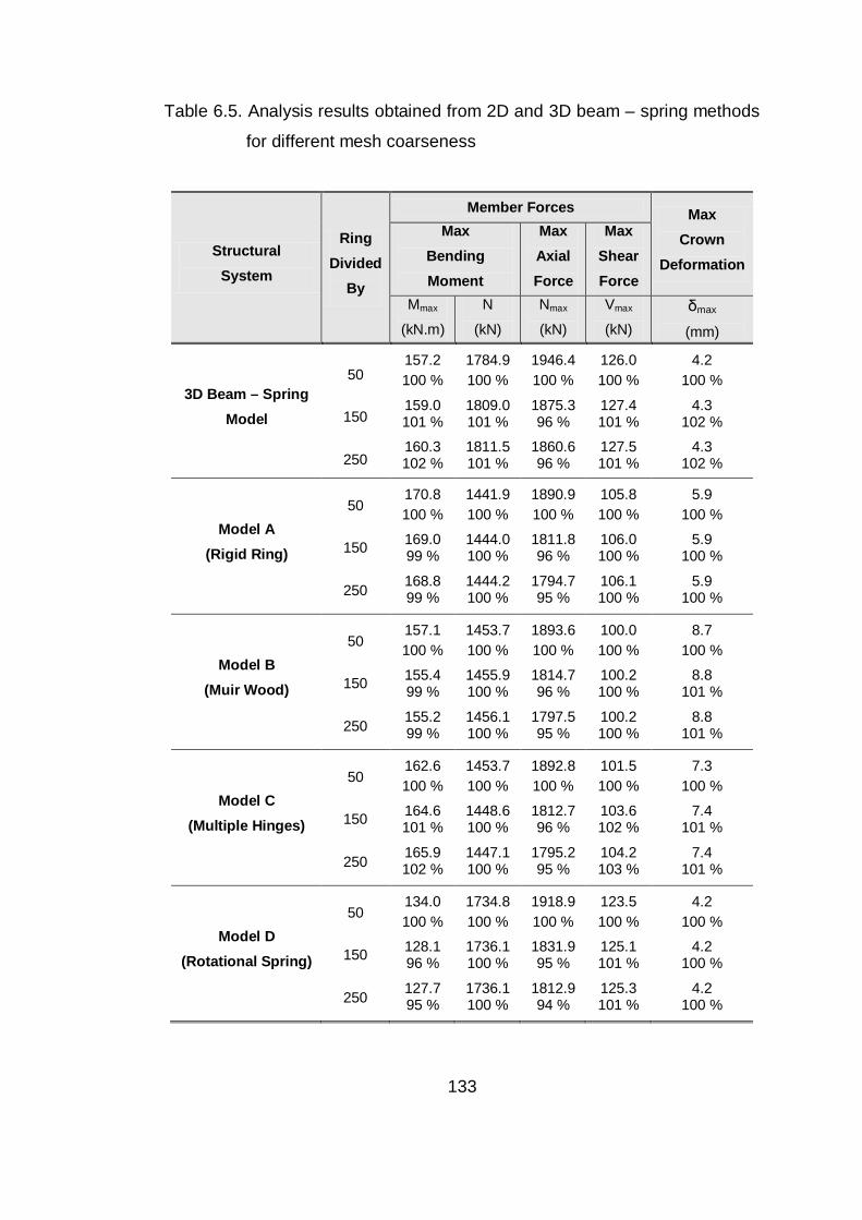
133

Table 6.5. Analysis results obtained from 2D and 3D beam – spring methods

for different mesh coarseness

Structural System

Ring Divided

By


Deformation

Max Bending Moment

Max Axial Force

Max Shear Force

Mmax

(kN.m) N

(kN) Nmax

(kN) Vmax

(kN) δmax (mm)

3D Beam – Spring Model

50

150

250

157.2 100 %

159.0 101 %

160.3 102 %

1784.9 100 %

1809.0 101 %

1811.5 101 %

1946.4 100 %

1875.3 96 %

1860.6 96 %

126.0 100 %

127.4 101 %

127.5 101 %

4.2 100 %

4.3 102 %

4.3 102 %


50

150

250

170.8 100 %

169.0 99 %

168.8 99 %

1441.9 100 %

1444.0 100 %

1444.2 100 %

1890.9 100 %

1811.8 96 %

1794.7 95 %

105.8 100 %

106.0 100 %

106.1 100 %

5.9 100 %

5.9 100 %

5.9 100 %

Model B (Muir Wood)

50

150

250

157.1 100 %

155.4 99 %

155.2 99 %

1453.7 100 %

1455.9 100 %

1456.1 100 %

1893.6 100 %

1814.7 96 %

1797.5 95 %

100.0 100 %

100.2 100 %

100.2 100 %

8.7 100 %

8.8 101 %

8.8 101 %


50

150

250

162.6 100 %

164.6 101 %

165.9 102 %

1453.7 100 %

1448.6 100 %

1447.1 100 %

1892.8 100 %

1812.7 96 %

1795.2 95 %

101.5 100 %

103.6 102 %

104.2 103 %

7.3 100 %

7.4 101 %

7.4 101 %


50

150

250

134.0 100 %

128.1 96 %

127.7 95 %

1734.8 100 %

1736.1 100 %

1736.1 100 %

1918.9 100 %

1831.9 95 %

1812.9 94 %

123.5 100 %

125.1 101 %

125.3 101 %

4.2 100 %

4.2 100 %

4.2 100 %

134

It is concluded from this comparison that mesh coarseness has not a

considerable effect on beam – spring analyses. Also, feasible mesh

coarseness can be provided by dividing segmental rings into a series of

beam elements having a length of nearly 0.5 m in order to obtain reasonable

results.

6.5. The Effect of Shear Spring Constant on Beam – Spring Analysis

In order to determine the sensitivity of shear spring constants, three 3D

BSMs with different shear spring constants have been employed and the

results are summarized in Table 6.6. The results obtained from 3D BSM with

a shear spring constant of 15000 kN/m are used as a base and they are

accepted as 100 % for a clear comparison.

Table 6.6. Analysis results obtained from 3D beam – spring methods for

three different shear spring constants

Structural System


Deformation

Max Bending Moment

Max Axial Force

Max Shear Force

Mmax

(kN.m) N

(kN) Nmax

(kN) Vmax

(kN) δmax (mm)

3D BSM (Ks = 15000 kN/m)

148.7 100 %

1759.3 100 %

1918.9 100 %

126.2 100 %

4.2 100 %

3D BSM (Ks = 20000 kN/m)

157.2 106 %

1784.9 101 %

1946.4 101 %

126.5 100 %

4.2 100 %

3D BSM (Ks = 25000 kN/m)

176.0 118 %

1857.4 106 %

2001.3 104 %

127.3 101 %

4.2 100 %

135

As seen in Table 6.6, 3D BSM with the highest shear spring constant gives

the maximum results for bending moment, axial force, and shear force.

Especially, difference in the maximum bending moment is 18 % between two

models having the maximum and minimum shear spring constants. The

reason is that as the shear spring constant increases, the load transfer

between the adjacent rings also increases. Therefore, higher load transfer

expectedly leads to increase in sectional forces. However, maximum crown

deformation is not affected by shear spring constants due to the harmonized

deformation pattern.

It can be concluded that shear spring constant which is a mechanical

property of circumferential joints has a notable effect on sectional forces;

especially on bending moment. Therefore, selecting a realistic shear spring

constant is essential for 3D BSMs.

6.6. The Effect of Segment Layout on Beam – Spring

Analysis Four possible segment arrangements shown in Figure 5.13 for a segmental

ring sequence are examined with 3D BSM in order to determine the effect of

segment layout on sectional forces and deformation of segmental linings.

The analysis results for four different segment layouts are given in Table 6.7.

For a clear comparison, the results of Layout 1 is selected as a base and

accepted as 100 %.

As shown in Table 6.7, maximum difference in results exists in bending

moments. Layout 4 has the most unfavorable configuration in terms of

bending moment and crown deformation. Since the longitudinal joint between

segment A and segment B is located very close to crown, Layout 4 gives the

maximum bending moment and crown deformation. Furthermore, axial forces

are in similar range and shear forces differ slightly.

136

Table 6.7. Analysis results obtained from 3D beam – spring methods for four

different segment configurations

Structural System


Deformation

Max Bending Moment

Max Axial Force

Max Shear Force

Mmax

(kN.m) N

(kN) Nmax

(kN) Vmax

(kN) δmax (mm)

3D BSM for (LAYOUT 1)

157.2 100 %

1784.9 100 %

1946.4 100 %

126.0 100 %

4.2 100 %


147.3 94 %

1756.0 98%

1914.4 98 %

111.6 89 %

4.7 110 %


130.7 83 %

1754.5 98 %

1913.1 98 %

120.4 96 %

4.2 100 %


175.2 111 %

1777.8 100 %

1940.1 100 %

134.5 107 %

4.9 117 %

The results show that segment layout in sequential rings is the other

geometrical parameter that affects the sectional forces and deformation;

especially bending moments. For that reason, different segment layouts for a

ring should be analyzed with 3D BSMs in order to determine the most

favorable segment configuration in the design of segmental linings.

137

CHAPTER 7

CONLUSION

The evaluation of 2D and 3D analysis methods proposed for the design of

segmental linings is performed by comparing the analysis results. The

influences of several factors such as joint stiffness, joint configuration, soil

stiffness, mesh coarseness, and different loading conditions are also

investigated using the Larsa4D structural analysis program. Based on the

evaluations given in the previous chapter, the following conclusions can be

achieved from this thesis study. The conclusions given below are obtained

from investigated cases for the selected tunnel section and loading

conditions.

• It is found that Elastic Equation Method underestimates sectional

forces up to 27 % in reference to 3D BSM for a regular load case.

• 2D BSMs are also found to underestimate sectional forces and

deformations up to 21 % and 106 %, respectively in accordance with

3D BSM for a regular load case.

• Results obtained from 2D and 3D BSMs representing the change in

the stiffness of surrounding soil differ up to 17 % for sectional forces.

• 2D and 3D BSMs simulating a TBM tunnel passing under a local

surcharge load calculate sectional forces varying up to 49 %.

138

• The mesh coarseness has not a considerable effect on the results

obtained from 2D and 3D BSMs. Accordingly, the length of beam

elements representing segments can be selected as 0.5 m on average

in order to obtain reasonable results.

• Bending moments obtained from 3D BSMs are found to be dependent

on shear spring constant. Therefore, selection of a proper shear spring

constant is a crucial point for the design of segmental linings.

• It can be concluded that segment configuration in sequential rings

considerably affects the sectional forces and deformations up to 34 %

and 17 %, respectively. Therefore, the most favorable segment

configuration can be determined with 3D BSMs.

• It can be indicated as a general conclusion that mechanical,

geometrical, and loading conditions to which tunnels can be exposed

both in longitudinal and circumferential directions may have significant

effects on the sectional forces and deformations of TBM segmental

linings.

139

REFERENCES

[1] Szechy K., The Art of Tunnelling, 2nd Ed., Akademiai Kiado, Budapest,

1973.

[2] O’Rourke T.D., ASCE Guidelines for Tunnel Lining Design, ASCE

Geotechnical Division, Virginia, 1984.

[3] Guglielmetti V., Grasso P., Mahtab A., Xu S., Mechanized Tunnelling

in Urban Areas: Design Methodology and Construction Control, Taylor

& Francis Group, London, UK, 2008.

[4] Möller S., Tunnel Induced Settlements and Structural Forces in

Linings, PhD Thesis, Stuttgart University, 2006.

[5] Megaw T.M., Bartlett J. V., Tunnels: Planning, Design, Construction,

Volume 1, Ellis Horwood Limited, West Sussex, 1981.

[6] Sinha R.S., Underground Structures - Design and Instrumentation,

Elsevier, The Netherlands, 1989.

[7] Maidl B., Herrenknecht M., Anheuser L., Mechanized Shield

Tunnelling, Ernst and Sohn, Berlin, 1995.

[8] Megaw T.M., Bartlett J. V., Tunnels: Planning, Design, Construction,

Volume 2, Ellis Horwood Limited, West Sussex, 1981.

140

[9] Kolymbas D., Tunnelling and Tunnel Mechanics - A Rational Approach

to Tunneling, Elsevier, Amsterdam, 2005.

[10] Sinha R.S., Underground Structure - Design and Construction,

Elsevier, The Netherlands, 1991.

[11] AFTES, New Recommendations on Choosing Mechanized Tunnelling

Techniques, French Tunnelling and Underground Engineering

Association, 2000.

[12] Richardson H.W., Mayo R.S., Practical Tunnel Driving, Mc. Graw Hill,

New York, 1947.

[13] Maidl B., Schmid L., Herrenknecht M., Hardrock Tunnel Boring

Machines, Ernst and Sohn, Berlin, 2008.

[14] Wittke W., Stability Analysis and Design for Mechanized Tunnelling,

Geotechnical Engineering in Research and Practice, WBI - Print 6,

Aachen, 2007.

[15] Girmscheid G., Schildvorgetriebener Tunnelbau in Heterogenem

Lokkergestein, ausgekleidet mit Stahlbetontübbingen, Teil 2: Aspekte

der Vortriebsmaschinen und Tragwerksplanung, Bautechnik 74, Heft 2,

1997.

[16] ITA - WG14, Recommendations and Guidelines for Tunnel Boring

Machines (TBMs), International Tunnelling Association, Working Group

No. 14 - Mechanized Tunnelling, 2000.

[17] Toan N. D., TBM and Lining – Essential Interfaces, Post Graduate Ms.

Thesis, Politecnico Di Torino, 2006.

141

[18] Kovari K., Ramoni M., Urban Tunnelling in Soft Ground Using TBM's,

Key Note Lecture at International Congress on Mechanized Tunnelling:

Challenging Case Histories, Politecnico di Torino, Italy, 2004.

[19] Herrenknecht AG, “http://www.herrenknecht.com/products/tunnel-

boring-machines.html”, last accessed on 11/01/2009.

[20] Haack A., Comparison Between Conventional Tunnel Driving Method

and TBM Drives - Worldwide Demand of Tunnel Constructions, Tunnel

Boring Machines - Trends in Design and Construction of Mechanized

Tunnelling, Hagenberg, Austria, 1995, Wagner & Schulter (eds),

Balkema/Rotterdam, 1996.

[21] Thewes M., Segment Linings for Shield Machines, International

Course on Shield Tunneling, Delft Geo Academy, The Netherlands,

2008.

[22] Herrenknecht M., Bappler K., Segmental Concrete Lining Design and

Installation, Soft Ground and Hard Rock Mechanical Tunneling

Technology Seminar, Colorado School of. Mines, 2003.

[23] ITA - WG2, Guidelines for the Design of Shield Tunnel Lining,

International Tunnelling Association, Working Group No. 2 – Research,

2000.

[24] JSCE, Japanese Standard for Shield Tunnelling, Japan Society of Civil

Engineers, The third edition, Tokyo, 1996.

[25] Duddeck H., Erdmann J., Structural Design Models for Tunnels,

Universitat Braunschweig, Germany, 1982.

http://www.herrenknecht.com/products/tunnel-boring-machines.html�

http://www.herrenknecht.com/products/tunnel-boring-machines.html�

142

[26] Schulze H., Duddeck H., Spannungen in Schildvorgetriebenen

Tunneln, Beton Stahlbetonb, Germany, 1964.

[27] Wood M., The Circular Tunnel in Elastic Ground, Geotechnique,

Volume 25, No. 1, 1975.

[28] AFTES – WG7, Considerations on the Usual Methods of Tunnel Lining

Design, French Tunneling and Underground Engineering Association,

Working Group No. 7 - Temporary Supports and Permanent Lining,

1993.

[29] Mashimo H., Ishimura T., Evaluation of the Load on a Shield Tunnel

Lining in Gravel, Public Works Research Institute, Independent

Administrative Institution, Tsukuba, Japan, 2003.

[30] Bickel J.0., Kuesel T.R., King E.H., Tunnel Engineering Handbook,

Chapman & Hall, United States of America, 1996.

[31] Koyama Y., Nishimura T., Design of Lining Segment of Shield Tunnel

Using a Beam – Spring Model, Quarterly Report of Railway Technical

Research Institute, Volume: 39(1), Japan.

[32] Lee K.M., Ge X.W., The Equivalence of a Jointed Shield-Driven Tunnel

Lining to a Continuous Ring Structure, Canadian Geotechnical Journal,

Volume 38, No. 3, 2001.

[33] Hefny A.M., Tan F.C., Macalevey N.F., Numerical Study on the

Behaviour of Jointed Tunnel Lining, Journal of The Institution of

Engineers, Volume 44, Issue 1, Singapore, 2004.

143

[34] Janssen P., Tragverhalten von Tunnelausbauten mit Gelenktubbings,

Report No. 83-41, University of Braunschweig, Department of Civil

Engineering, Institute for Structural Analysis, 1983.

[35] Leonhard F., Reimann H., Betongelenke, Der Bauingenieur, Volume

41, 1966.

[36] Klappers C., Gruebl F., Ostermeier B., Structural Analysis of

Segmental Lining – Coupled Beam and Spring Analyses Versus 3D

FEM Calculations with Shell Elements, Tunneling and Underground

Space Technology, Volume 21, Issues 3-4, 1999.

[37] Wang J.J., The Design Considerations for the Segmental Lining of the

Hsuehshan Tunnel, International Symposium on Design, Construction

and Operation of Long Tunnels, Taiwan, 2005.

[38] Koyama Y., Study on the Improvement of Design Method of Segments

for Shield-Driven Tunnels, RTRI Report: Special No. 33, 2000.

[39] Koyama Y., Present Status and Technology of Shield Tunneling

Method in Japan, Tunneling and Underground Space Technology,

Volume 18, 2003.

[40] Gioda G., Swoboda G., Developments and applications of the

numerical analysis of tunnels in continuous media, International

Journal for Numerical and Analytical Methods in Geomechanics,

Volume 23, 1999.

[41] Blom C.B.M., Horst E.J., Jovanovic P.S., Three-Dimensional Structural

Analyses of the Shield-Driven “Green Heart” Tunnel of the High-Speed

144

Line South, Tunneling and Underground Space Technology, Volume

14, No. 2, 1999.

[42] BTS - ICE, Tunnel Lining Design Guide, The British Tunneling Society

and Institution of Civil Engineers, Thomas Telford, London, 2004.

[43] AFTES, Recommendations for The Design, Sizing and Construction

of Precast Concrete Segments Installed at the Rear of a Tunnel

Boring Machine (TBM), French Tunneling and Underground

Engineering Association, Version 1, 1997.

145

APPENDIX A

WORKING SHEETS FOR THE ANALYSIS WITH ELASTIC EQUATION METHOD

Input, load conditions, and member forces sheets developed for the analysis

with Elastic Equation Method by using Microsoft Excel 2003 and Macro

Visual Basic applications are given in the following pages. Input sheet

includes geometrical, material, and geotechnical properties of the problem.

Calculations of loads and member forces are also provided in load conditions

sheets and member forces sheet, respectively.

Figu

re A

.1. I

nput

she

et fo

r the

ana

lysi

s w

ith E

last

ic E

quat

ion

Met

hod

146

Figu

re A

.2. L

oad

cond

ition

s sh

eet 1

for t

he a

naly

sis

with

Ela

stic

Equ

atio

n M

etho

d

147

Figu

re A

.3. L

oad

cond

ition

s sh

eet 2

for t

he a

naly

sis

with

Ela

stic

Equ

atio

n M

etho

d

148

Figu

re A

.4. M

embe

r for

ces

shee

t for

the

anal

ysis

with

Ela

stic

Equ

atio

n M

etho

d

149

150

APPENDIX B

SHEAR SPRING CONSTANTS FOR 2D AND 3D BSMs

0

20,000

40,000

60,000

80,000

100,000

120,000

140,000

-0.08 -0.06 -0.04 -0.02 0.00 0.02 0.04 0.06 0.08M/N

Rig

idity

(kN

m/r

ad)

Rotational Rigidity(n-1). Iterationn. Iteration

Figure B.1. Rotational Stiffness vs. M/N diagram for 2D BSM in Case 1

0

20,000

40,000

60,000

80,000

100,000

120,000

140,000

-0.08 -0.06 -0.04 -0.02 0.00 0.02 0.04 0.06 0.08M/N

Rigi

dity

(kNm

/rad)


Figure B.2. Rotational Stiffness vs. M/N diagram for 3D BSM in Case 1

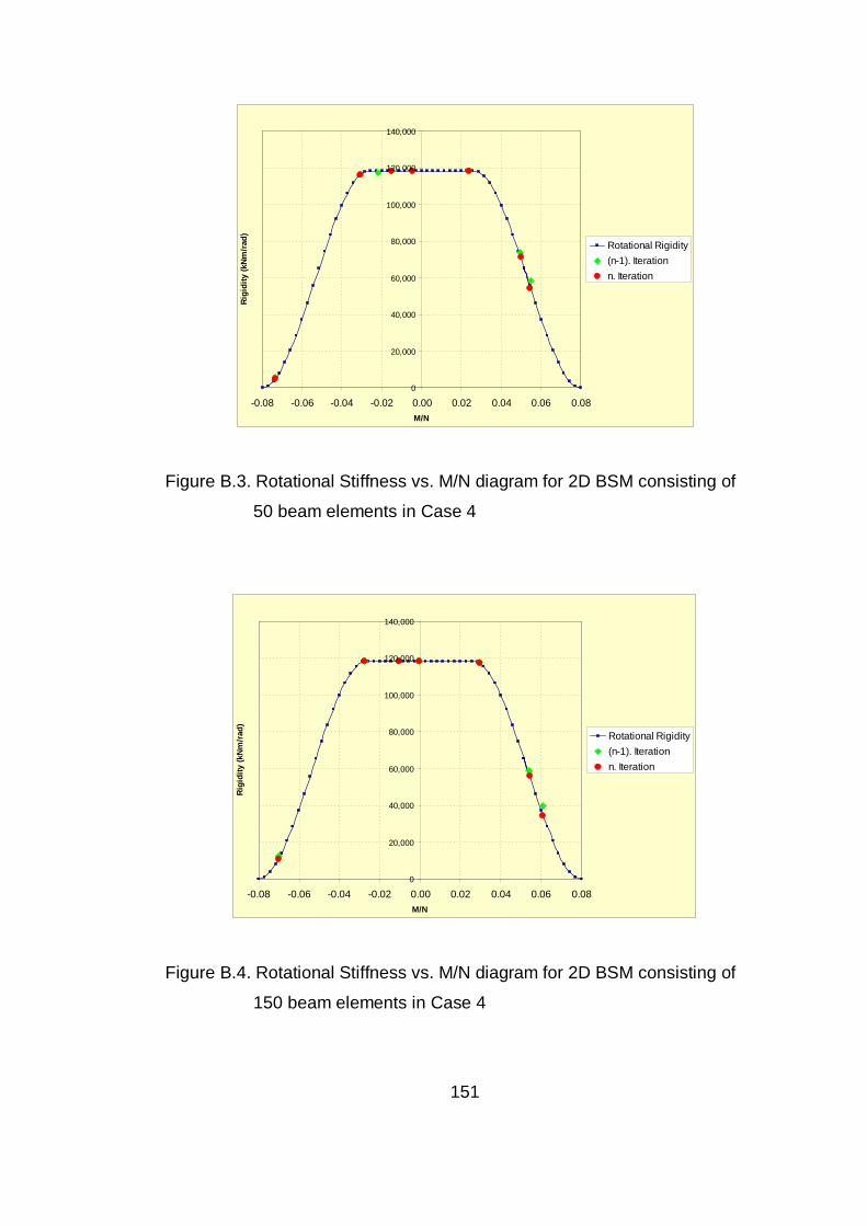
151

0

20,000

40,000

60,000

80,000

100,000

120,000

140,000

-0.08 -0.06 -0.04 -0.02 0.00 0.02 0.04 0.06 0.08M/N

Rig

idity

(kN

m/r

ad)


Figure B.3. Rotational Stiffness vs. M/N diagram for 2D BSM consisting of

50 beam elements in Case 4

0

20,000

40,000

60,000

80,000

100,000

120,000

140,000

-0.08 -0.06 -0.04 -0.02 0.00 0.02 0.04 0.06 0.08M/N

Rigi

dity

(kNm

/rad)




152

0

20,000

40,000

60,000

80,000

100,000

120,000

140,000

-0.08 -0.06 -0.04 -0.02 0.00 0.02 0.04 0.06 0.08M/N

Rig

idity

(kN

m/m

/rad

)Rotational Rigidity(n-1). Iterationn. Iteration



0

20,000

40,000

60,000

80,000

100,000

120,000

140,000

-0.08 -0.06 -0.04 -0.02 0.00 0.02 0.04 0.06 0.08M/N

Rigi

dity

(kNm

/rad)


Figure B.6. Rotational Stiffness vs. M/N diagram for 3D BSM consisting of 50

beam elements in Case 4

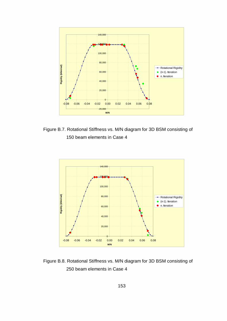
153

-20,000

0

20,000

40,000

60,000

80,000

100,000

120,000

140,000

-0.08 -0.06 -0.04 -0.02 0.00 0.02 0.04 0.06 0.08

M/N

Rig

idity

(kN

m/r

ad)




0

20,000

40,000

60,000

80,000

100,000

120,000

140,000

-0.08 -0.06 -0.04 -0.02 0.00 0.02 0.04 0.06 0.08M/N

Rigi

dity

(kNm

/rad

)




154

0

20,000

40,000

60,000

80,000

100,000

120,000

140,000

-0.08 -0.06 -0.04 -0.02 0.00 0.02 0.04 0.06 0.08M/N

Rig

idity

(kN

m/r

ad)


Figure B.9. Rotational Stiffness vs. M/N diagram for 3D BSM (Ks=15000

kN/m) in Case 5

0

20,000

40,000

60,000

80,000

100,000

120,000

140,000

-0.08 -0.06 -0.04 -0.02 0.00 0.02 0.04 0.06 0.08M/N

Rigi

dity

(kNm

/rad

)



kN/m) in Case 5

155

0

20,000

40,000

60,000

80,000

100,000

120,000

140,000

-0.08 -0.06 -0.04 -0.02 0.00 0.02 0.04 0.06 0.08M/N

Rig

idity

(kN

m/r

ad)



kN/m) in Case 5

0

20,000

40,000

60,000

80,000

100,000

120,000

140,000

-0.08 -0.06 -0.04 -0.02 0.00 0.02 0.04 0.06 0.08M/N

Rig

idity

(kN

m/r

ad)


Figure B.12. Rotational Stiffness vs. M/N diagram for 3D BSM (Layout 1) in

Case 6

156

0

20,000

40,000

60,000

80,000

100,000

120,000

-0.08 -0.06 -0.04 -0.02 0.00 0.02 0.04 0.06 0.08M/N

Rigi

dity

(kNm

/rad)



Case 6

0

20,000

40,000

60,000

80,000

100,000

120,000

140,000

-0.08 -0.06 -0.04 -0.02 0.00 0.02 0.04 0.06 0.08M/N

Rig

idity

(kN

m/r

ad)



Case 6

157

0

20,000

40,000

60,000

80,000

100,000

120,000

140,000

-0.08 -0.06 -0.04 -0.02 0.00 0.02 0.04 0.06 0.08M/N

Rigi

dity

(kNm

/rad)



Case 6

Index

Documents

Transcript of Index