Independent component analysis via nonparametric maximum ...my2550/papers/ica.final.pdf · ICA VIA...
30
The Annals of Statistics 2012, Vol. 40, No. 6, 2973–3002 DOI: 10.1214/12-AOS1060 © Institute of Mathematical Statistics, 2012 INDEPENDENT COMPONENT ANALYSIS VIA NONPARAMETRIC MAXIMUM LIKELIHOOD ESTIMATION BY RICHARD J. SAMWORTH 1 AND MING YUAN 2 University of Cambridge and Georgia Institute of Technology Independent Component Analysis (ICA) models are very popular semi- parametric models in which we observe independent copies of a random vec- tor X = AS , where A is a non-singular matrix and S has independent compo- nents. We propose a new way of estimating the unmixing matrix W = A −1 and the marginal distributions of the components of S using nonparamet- ric maximum likelihood. Specifically, we study the projection of the em- pirical distribution onto the subset of ICA distributions having log-concave marginals. We show that, from the point of view of estimating the unmixing matrix, it makes no difference whether or not the log-concavity is correctly specified. The approach is further justified by both theoretical results and a simulation study. 1. Introduction. In recent years, Independent Component Analysis (ICA) has seen an explosion in its popularity in diverse fields such as signal processing, ma- chine learning and medical imaging, to name a few. For a wide-ranging list of algorithms and applications of ICA, see the monograph by Hyvärinen, Karhunen and Oja (2001). In the ICA paradigm, one observes a random vector X ∈ R d that can be expressed as a non-singular linear transformation of d mutually indepen- dent latent factors S 1 ,...,S d ; thus, X = AS , where S = (S 1 ,...,S d ) T and A is a d × d full rank matrix often referred to as the mixing matrix. As such, ICA postu- lates the following model for the probability distribution P of X: for any Borel set B in R d , P(B) = d j =1 P j ( w T j B ) , where W = (w 1 ,...,w d ) T = A −1 is the so-called unmixing matrix and P 1 ,...,P d are the univariate probability distributions of the latent factors S 1 ,...,S d , respec- tively. The goal of ICA, as in other blind source separation problems, is to infer, from a sample x 1 ,..., x n of independent observations of X, the independent factors Received June 2012; revised October 2012. 1 Supported in part by a Leverhulme Research Fellowship and an EPSRC Early Career Fellowship. 2 Supported in part by NSF Career Award DMS-0846234. MSC2010 subject classifications. 62G07. Key words and phrases. Blind source separation, density estimation, independent component analysis, log-concave projection, nonparametric maximum likelihood estimator. 2973
Transcript of Independent component analysis via nonparametric maximum ...my2550/papers/ica.final.pdf · ICA VIA...

The Annals of Statistics2012, Vol. 40, No. 6, 2973–3002DOI: 10.1214/12-AOS1060© Institute of Mathematical Statistics, 2012
INDEPENDENT COMPONENT ANALYSIS VIA NONPARAMETRICMAXIMUM LIKELIHOOD ESTIMATION
BY RICHARD J. SAMWORTH1 AND MING YUAN2
University of Cambridge and Georgia Institute of Technology
Independent Component Analysis (ICA) models are very popular semi-parametric models in which we observe independent copies of a random vec-tor X = AS, where A is a non-singular matrix and S has independent compo-nents. We propose a new way of estimating the unmixing matrix W = A−1
and the marginal distributions of the components of S using nonparamet-ric maximum likelihood. Specifically, we study the projection of the em-pirical distribution onto the subset of ICA distributions having log-concavemarginals. We show that, from the point of view of estimating the unmixingmatrix, it makes no difference whether or not the log-concavity is correctlyspecified. The approach is further justified by both theoretical results and asimulation study.
1. Introduction. In recent years, Independent Component Analysis (ICA) hasseen an explosion in its popularity in diverse fields such as signal processing, ma-chine learning and medical imaging, to name a few. For a wide-ranging list ofalgorithms and applications of ICA, see the monograph by Hyvärinen, Karhunenand Oja (2001). In the ICA paradigm, one observes a random vector X ∈ R
d thatcan be expressed as a non-singular linear transformation of d mutually indepen-dent latent factors S1, . . . , Sd ; thus, X = AS, where S = (S1, . . . , Sd)T and A is ad × d full rank matrix often referred to as the mixing matrix. As such, ICA postu-lates the following model for the probability distribution P of X: for any Borel setB in R
d ,
P(B) =d∏
j=1
Pj
(wT
j B),
where W = (w1, . . . ,wd)T = A−1 is the so-called unmixing matrix and P1, . . . ,Pd
are the univariate probability distributions of the latent factors S1, . . . , Sd , respec-tively.
The goal of ICA, as in other blind source separation problems, is to infer, froma sample x1, . . . ,xn of independent observations of X, the independent factors
Received June 2012; revised October 2012.1Supported in part by a Leverhulme Research Fellowship and an EPSRC Early Career Fellowship.2Supported in part by NSF Career Award DMS-0846234.MSC2010 subject classifications. 62G07.Key words and phrases. Blind source separation, density estimation, independent component
analysis, log-concave projection, nonparametric maximum likelihood estimator.
2973

2974 R. J. SAMWORTH AND M. YUAN
s1 = Wx1, . . . , sn = Wxn or, equivalently, the unmixing matrix W . This task istypically accomplished by first postulating a certain parametric family for themarginal probability distributions P1, . . . ,Pd , and then optimising a contrast func-tion involving (W,P1, . . . ,Pd), for example, Karvanen and Koivunen (2002). Thecontrast functions are often chosen to represent the mutual information as mea-sured by Kullback–Leibler divergence or maximum entropy, or non-Gaussianityas measured by kurtosis or negentropy. Alternatively, in recent years, methodsfor ICA have also been developed which assume P1, . . . ,Pd have smooth (log)densities, for example, Bach and Jordan (2002), Hastie and Tibshirani (2003b),Samarov and Tsybakov (2004), Chen and Bickel (2006) and Ilmonen and Paindav-eine (2011). Although more flexible than their aforementioned parametric peers,there remain unsettling questions about what happens if the smoothness assump-tions on the marginal densities are violated, which may occur, in particular, whensome of the marginal probability distributions P1, . . . ,Pd have atoms. Another is-sue is that, in common with most other smoothing methods, a choice of tuningparameters is required to balance the fidelity to the observed data and the smooth-ness of the estimated marginal densities, and it is notoriously difficult to selectthese tuning parameters appropriately in practice.
In this paper, we argue that these assumptions and tuning parameters are unnec-essary, and propose a new paradigm for ICA, based on the notion of nonparametricmaximum likelihood, that is free of these burdens. In fact, we show that the usualnonparametric (empirical) likelihood approach does not work in this context, andinstead we proceed under the working assumption that the marginal distributionsof S1, . . . , Sd are log-concave. More specifically, we propose to estimate W bymaximising
log|detW | + 1
n
n∑i=1
d∑j=1
logfj
(wT
j xi
)
over all d × d non-singular matrices W = (w1, . . . ,wd)T and univariate log-concave densities f1, . . . , fd . Remarkably, from the point of view of estimatingthe unmixing matrix W , it turns out that it makes no difference whether or not thishypothesis of log-concavity is correctly specified.
The key to understanding how our approach works is to study what we call thelog-concave ICA projection of a distribution on R
d onto the set of densities thatsatisfy the ICA model with log-concave marginals. In Section 2.1 below, we definethis projection carefully and give necessary and sufficient conditions for it to makesense. In Section 2.2, we prove that the log-concave projection of a distributionfrom the ICA model preserves both the ICA structure and the unmixing matrix.Finally, in Section 2.3, we derive a continuity property of log-concave ICA projec-tions, which turns out to be important for understanding the theoretical propertiesof our ICA procedure.

ICA VIA NONPARAMETRIC MAXIMUM LIKELIHOOD 2975
Our ICA estimating procedure uses the log-concave ICA projection of the em-pirical distribution of the data, and is studied in Section 3. After explaining whythe usual empirical likelihood approach cannot be used, we prove the consistencyof our method. We also present an iterative algorithm for the computation of ourestimator. Our simulation studies in Section 4 confirm our theoretical results andshow that the proposed method compares favourably with existing methods. Proofsare deferred to Section 5.
To conclude this section, we remark that in addition to the previous literaturealready cited, further approaches to ICA have been proposed that use a choice oftwo scatter (or shape) matrices [Nordhausen, Oja and Ollila (2011), Oja, Sirkiäand Eriksson (2006), Ollila, Oja and Koivunen (2008)]. To uniquely define theunmixing matrix, one scatter matrix (often chosen based on fourth moments) musttake distinct values on its main diagonal, which rules out situations where twoof the marginal distributions P1, . . . ,Pd are the same. Nevertheless, under further(e.g., moment) assumptions, root-n consistency and asymptotic normality resultsfor estimates of the unmixing matrix under correct model specification have beenobtained [e.g., Ilmonen, Nevalainen and Oja (2010)].
2. Log-concave ICA projections.
2.1. Notation and overview. Let Pk be the set of probability distributions P
on Rk satisfying
∫Rk ‖x‖dP (x) < ∞ and P(H) < 1 for all hyperplanes H , that
is, the probability measures in Rk that have finite mean and are not supported in
a translate of a lower-dimensional linear subspace of Rk . Here and throughout,
‖ · ‖ denotes the Euclidean norm on Rk , and we will be interested in the cases
k = 1 and k = d . Further, let W denote the set of non-singular d × d real matrices.We use upper case letters to denote matrices in W , and the corresponding lowercase letters with subscripts to denote rows: thus, wT
j is the j th row of W ∈ W . Let
Bk denote the class of Borel sets on Rk . Then the ICA model P ICA
d is defined tobe the set of P ∈ Pd of the form
P(B) =d∏
j=1
Pj
(wT
j B) ∀B ∈ Bd(1)
for some W ∈ W and P1, . . . ,Pd ∈ P1. As shown by Dümbgen, Samworth andSchuhmacher [(2011), Theorem 2.2], the condition P ∈ Pd is necessary and suffi-cient for the existence of a unique upper semi-continuous and log-concave densitythat is the closest to P in the Kullback–Leibler sense. More precisely, let Fk de-note the class of all upper semi-continuous, log-concave densities with respect tothe Lebesgue measure on R
k . Then the projection ψ∗ : Pd → Fd given by
ψ∗(P ) = arg maxf ∈Fd
∫Rd
logf dP

2976 R. J. SAMWORTH AND M. YUAN
is well defined and surjective. In what follows, we refer to ψ∗ as the log-concaveprojection operator and f ∗ := ψ∗(P ) as the log-concave projection of P . By aslight abuse of notation, we also use ψ∗ to denote the log-concave projection fromP1 to F1.
Although the log-concave projection operator does play a role in this paper, ourmain interest is in a different projection, onto the subset of Fd consisting of thosedensities that belong to the ICA model. This class is given by
F ICAd =
{f ∈ Fd :f (x) = |detW |
d∏j=1
fj
(wT
j x)
(2)
with W ∈ W, f1, . . . , fd ∈ F1
}.
Note that, in this representation, if X has density f ∈ F ICAd , then wT
j X has den-sity fj . The corresponding log-concave ICA projection operator ψ∗∗(·) is definedfor any distribution P on R
d by
ψ∗∗(P ) = arg maxf ∈F ICA
d
∫Rd
logf dP.
We also write L∗∗(P ) = supf ∈F ICAd
∫Rd logf dP .
PROPOSITION 1. (1) If∫Rd ‖x‖dP (x) = ∞, then L∗∗(P ) = −∞ and
ψ∗∗(P ) = F ICAd .
(2) If∫Rd ‖x‖dP (x) < ∞, but P(H) = 1 for some hyperplane H , then
L∗∗(P ) = ∞ and ψ∗∗(P ) = ∅.(3) If P ∈ Pd , then L∗∗(P ) ∈ R and ψ∗∗(P ) defines a non-empty, proper subset
of F ICAd .
In view of Proposition 1, and to avoid lengthy discussion of trivial exceptionalcases, we henceforth consider ψ∗∗(·) as being defined on Pd . In contrast to ψ∗(P ),which defines a unique element of Fd , the log-concave ICA projection operatorψ∗∗(P ) may not define a unique element of F ICA
d , even for P ∈ Pd . For instance,consider the situation where P is the uniform distribution on the closed unit diskin R
2 equipped with the Euclidean norm. Here, the spherical symmetry meansthat the choice of W ∈ W is not uniquely defined. In fact, after a straightforwardcalculation, it can be shown that ψ∗∗(P ) includes all f ∈ F ICA
2 , where, in therepresentation (2), W is an orthogonal matrix and f1, f2 ∈ F1 are given by f1(x) =f2(x) = 2
π(1 − x2)1/21{x∈[−1,1]}. It is certainly possible to make different choices
of W that yield different elements of F ICA2 . This example shows that, in general,
we must think of ψ∗∗(P ) as defining a subset of F ICAd .

ICA VIA NONPARAMETRIC MAXIMUM LIKELIHOOD 2977
The relationship between the spaces introduced above and the projection oper-ators is illustrated in the diagram below:
Pdψ∗
−→ Fd
ψ∗∗↘
P ICAd
ψ∗∗|P ICAd−→ F ICA
d .
Our next subsection studies the restriction of ψ∗∗ to P ICAd , denoted ψ∗∗|P ICA
d; Sec-
tion 2.2 examines ψ∗∗ more generally as a map on Pd .
2.2. Log-concave projections of the ICA model. Our first result in this subsec-tion characterises ψ∗∗|P ICA
d.
THEOREM 2. If P ∈ P ICAd , then ψ∗∗(P ) defines a unique element of F ICA
d .The map ψ∗∗|P ICA
dis surjective, and coincides with ψ∗|P ICA
d. Moreover, suppose
that P ∈ P ICAd , so that
P(B) =d∏
j=1
Pj
(wT
j B) ∀B ∈ Bd
for some W ∈ W and P1, . . . ,Pd ∈ P1. Then f ∗∗ = ψ∗∗(P ) can be written as
f ∗∗(x) = |detW |d∏
j=1
f ∗j
(wT
j x),
where f ∗j = ψ∗(Pj ).
It is interesting to observe that the log-concave projection operator ψ∗ preservesthe ICA structure. But perhaps the most important aspect of this result is the factthat the same unmixing matrix W can be used to represent both the original ICAmodel and its log-concave projection. This observation lies at the heart of the ra-tionale for our approach to ICA.
A remaining concern is that the unmixing matrix may not be identifiable. For in-stance, applying the same permutation to the rows of W and the vector of marginaldistributions (P1, . . . ,Pd) leaves the distribution unchanged; similarly, the sameeffect occurs if we multiply any of the rows of W by a scaling factor and applythe corresponding scaling factor to the relevant marginal distribution. The ques-tion of identifiability for ICA models was first addressed by Comon (1994), whoassumed that W is orthogonal, and was settled in the general case by Eriksson
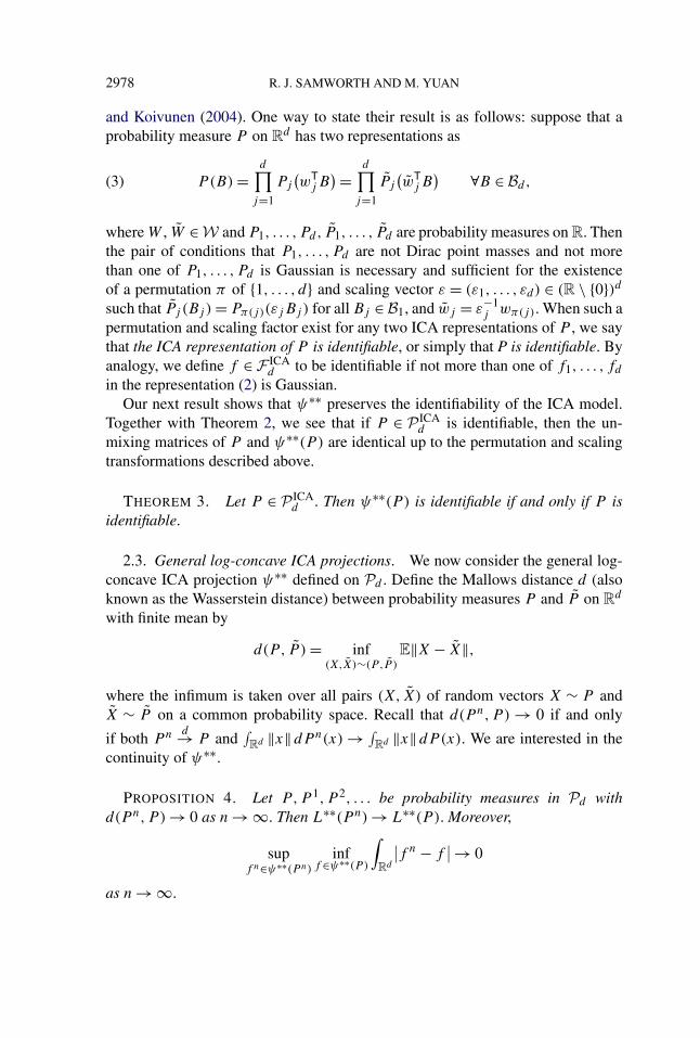
2978 R. J. SAMWORTH AND M. YUAN
and Koivunen (2004). One way to state their result is as follows: suppose that aprobability measure P on R
d has two representations as
P(B) =d∏
j=1
Pj
(wT
j B) =
d∏j=1
Pj
(wT
j B) ∀B ∈ Bd,(3)
where W , W ∈ W and P1, . . . ,Pd, P1, . . . , Pd are probability measures on R. Thenthe pair of conditions that P1, . . . ,Pd are not Dirac point masses and not morethan one of P1, . . . ,Pd is Gaussian is necessary and sufficient for the existenceof a permutation π of {1, . . . , d} and scaling vector ε = (ε1, . . . , εd) ∈ (R \ {0})dsuch that Pj (Bj ) = Pπ(j)(εjBj ) for all Bj ∈ B1, and wj = ε−1
j wπ(j). When such apermutation and scaling factor exist for any two ICA representations of P , we saythat the ICA representation of P is identifiable, or simply that P is identifiable. Byanalogy, we define f ∈ F ICA
d to be identifiable if not more than one of f1, . . . , fd
in the representation (2) is Gaussian.Our next result shows that ψ∗∗ preserves the identifiability of the ICA model.
Together with Theorem 2, we see that if P ∈ P ICAd is identifiable, then the un-
mixing matrices of P and ψ∗∗(P ) are identical up to the permutation and scalingtransformations described above.
THEOREM 3. Let P ∈ P ICAd . Then ψ∗∗(P ) is identifiable if and only if P is
identifiable.
2.3. General log-concave ICA projections. We now consider the general log-concave ICA projection ψ∗∗ defined on Pd . Define the Mallows distance d (alsoknown as the Wasserstein distance) between probability measures P and P on R
d
with finite mean by
d(P, P ) = inf(X,X)∼(P,P )
E‖X − X‖,
where the infimum is taken over all pairs (X, X) of random vectors X ∼ P andX ∼ P on a common probability space. Recall that d(P n,P ) → 0 if and only
if both P n d→ P and∫Rd ‖x‖dP n(x) → ∫
Rd ‖x‖dP (x). We are interested in thecontinuity of ψ∗∗.
PROPOSITION 4. Let P,P 1,P 2, . . . be probability measures in Pd withd(P n,P ) → 0 as n → ∞. Then L∗∗(P n) → L∗∗(P ). Moreover,
supf n∈ψ∗∗(P n)
inff ∈ψ∗∗(P )
∫Rd
∣∣f n − f∣∣ → 0
as n → ∞.

ICA VIA NONPARAMETRIC MAXIMUM LIKELIHOOD 2979
The second part of this proposition says that any element of ψ∗∗(P n) is ar-bitrarily close in total variation distance to some element of ψ∗∗(P ) once n issufficiently large. In the special case where ψ∗∗(P ) consists of only a single ele-ment, we can say more. It is convenient to let �d denote the set of permutations
of {1, . . . , d}, and write (W,f1, . . . , fd)ICA∼ f if W ∈ W and f1, . . . , fd ∈ F1 can
be used to give an ICA representation of f ∈ F ICAd in (2). Similarly, we write
(W,P1, . . . ,Pd)ICA∼ P if W ∈ W and P1, . . . ,Pd ∈ P1 represent P ∈ P ICA
d in (1).
THEOREM 5. Suppose that P ∈ P ICAd , and write f ∗∗ = ψ∗∗(P ). If P 1,
P 2, . . . ∈ Pd are such that d(P n,P ) → 0, then
supf n∈ψ∗∗(P n)
∫Rd
∣∣f n − f ∗∗∣∣ → 0.
Suppose further that P is identifiable and that (W,P1, . . . ,Pd)ICA∼ P . Then
supf n∈ψ∗∗(P n)
sup(Wn,f n
1 ,...,f nd )
ICA∼ f n
infπn∈�d
infεn
1 ,...,εnd∈R\{0}
{∥∥(εnj
)−1wn
πn(j) − wj
∥∥
+∫ ∞−∞
∣∣∣∣εnj
∣∣f nπn(j)
(εnj x
) − f ∗j (x)
∣∣dx
}
→ 0
for each j = 1, . . . , d , where f ∗j = ψ∗(Pj ). As a consequence, for sufficiently
large n, every f n ∈ ψ∗∗(P n) is identifiable.
The convergence statement in Theorem 5 is quite complicated, partly becauseof the need to deal with possible reordering and/or scaling of the rows of the un-mixing matrices. An alternative approach, as adopted in Ilmonen and Paindaveine(2011), for instance, would be to study a particular representative of the equiva-lence class of unmixing matrices that can be used to represent a given distributionin F ICA
d . Our main reason for choosing this presentation was to make clear that thesame permutation and scaling yields simultaneous convergence of the log-concaveprojections of the marginal densities.
The first part of Theorem 5 shows that if P ∈ P ICAd and P ∈ Pd are close in
Mallows distance, then every f ∈ ψ∗∗(P ) is close to the corresponding (unique)log-concave ICA projection f = ψ∗∗(P ) in total variation distance. The secondpart shows further that if P is identifiable, then up to permutation and scaling,every f ∈ ψ∗∗(P ) and every choice of unmixing matrix W and marginal densitiesf1, . . . , fd in the ICA representation of f is close to the unmixing matrix W andmarginal densities f1, . . . , fd in the ICA representation of f .

2980 R. J. SAMWORTH AND M. YUAN
To conclude this subsection, we remark that, by analogy with the situation whenP ∈ P ICA
d described in Theorem 2, if P ∈ Pd and X ∼ P , any f ∗∗ ∈ ψ∗∗(P ) canbe written as
f ∗∗(x) = |detW |d∏
j=1
f ∗j
(wT
j x)
for some W ∈ W , where f ∗j = ψ∗(Pj ) and Pj is the marginal distribution of
wTj X. This observation reduces the maximisation problem involved in computing
ψ∗∗(P ) to a finite-dimensional one (over W ∈ W ), and follows because
supf ∈F ICA
d
∫Rd
logf dP
= supW∈W
supf1,...,fd∈F1
{log |detW | +
d∑j=1
∫Rd
logfj
(wT
j x)dP (x)
}
= supW∈W
{log |detW | +
d∑j=1
∫Rd
logf ∗j
(wT
j x)dP (x)
}.
3. Nonparametric maximum likelihood estimation for ICA models. Weare now in position to study the proposed nonparametric maximum likelihood es-timator.
3.1. Estimating procedure and theoretical properties. Assume x1,x2, . . . areindependent copies of a random vector X ∈ R
d satisfying the ICA model. Thus,X = AS, where A = W−1 ∈ W and S = (S1, . . . , Sd)T has independent compo-nents. In this section, we study a nonparametric maximum likelihood estimator ofW and the marginal distributions P1, . . . ,Pd of S1, . . . , Sd based on x1, . . . ,xn,where n ≥ d + 1.
We start by noting that the usual nonparametric maximum likelihood estimatedoes not work. Indeed, in the spirit of empirical likelihood [Owen (1990)], itwould suffice to consider, for a given W = (w1, . . . ,wd)T ∈ W , estimates Pj ofthe marginal distribution Pj , supported on wT
j x1, . . . ,wTj xn. This leads to the non-
parametric likelihood
L(W, P1, . . . , Pd) =n∏
i=1
d∏j=1
pij ,(4)
where pij = Pj (wTj xi ). Let J denote a subset of (d + 1) distinct indices in
{1, . . . , n}, and let XJ denote the d × (d + 1) matrix obtained by extracting thecolumns of X = (x1, . . . ,xn) with indices in J . Now let X(−j) denote the d × d
matrix obtained by removing the j th column of XJ . Let WJ ∈ W have j th row

ICA VIA NONPARAMETRIC MAXIMUM LIKELIHOOD 2981
wj = (X−1(−j))
T1d , for j = 1, . . . , d , where 1d is a d-vector of ones. We say thatx1, . . . ,xn are in general position if, whenever we take a n × r matrix M of fullrank, where every column of M contains exactly two non-zero entries, namely, a 1and a −1, and define Y = (y1, . . . ,yr ) by Y = XM, then Y has full rank. Our nextresult shows that if x1, . . . ,xn are in general position, then every WJ correspondsto a maximiser of the nonparametric likelihood (4).
PROPOSITION 6. Suppose that x1, . . . ,xn are in general position. Then forany choice J of (d + 1) distinct indices in {1, . . . , n}, there exist P1, . . . , Pd ∈ P1such that (WJ , P1, . . . , Pd) maximises L(·).
If X has a density with respect to the Lebesgue measure on Rd , then x1, . . . ,xn
are in general position with probability 1. On the other hand, there is no reason fordifferent choices of J to yield similar estimates WJ , so we cannot hope for suchan empirical likelihood-based procedure to be consistent.
As a remedy, we propose to estimate P 0 ∈ P ICAd by ψ∗∗(P n), where P n denotes
the empirical distribution of x1, . . . ,xn ∼ P 0. More explicitly, we estimate theunmixing matrix and the marginals by maximising the log-likelihood
�n(W,f1, . . . , fd) = �n(W,f1, . . . , fd;x1, . . . ,xn)(5)
= log |detW | + 1
n
n∑i=1
d∑j=1
logfj
(wT
j xi
)
over W ∈ W and f1, . . . , fd ∈ F1. Note from Proposition 1 that ψ∗∗(P n) existsas a proper subset of F ICA
d once the convex hull of x1, . . . ,xn is d-dimensional,which happens with probability 1 for sufficiently large n. As a direct consequenceof Theorem 5 and the fact that d(P n,P 0)
a.s.→ 0, we have the following consistencyresult.
COROLLARY 7. Suppose that P 0 ∈ P ICAd is identifiable and is represented
by W 0 ∈ W and P 01 , . . . ,P 0
d ∈ P1. Then for any maximiser (W n, f n1 , . . . , f n
d ) of�n(W,f1, . . . , fd) over W ∈ W and f1, . . . , fd ∈ F1, there exist a permutation πn
of {1, . . . , d} and scaling factors εn1 , . . . , εn
d ∈ R \ {0} such that
(εnj
)−1wn
πn(j)
a.s.→ w0j and
∫ ∞−∞
∣∣∣∣εnj
∣∣f nπn(j)
(εnj x
) − f ∗j (x)
∣∣dxa.s.→ 0
for j = 1, . . . , d , where f ∗j = ψ∗(P 0
j ).
3.2. Pre-whitening. Pre-whitening is a standard pre-processing technique inthe ICA literature; see Hyvärinen, Karhunen and Oja [(2001), pages 140 and 141]or Chen and Bickel (2005). In this subsection, we explain the rationale for pre-whitening and the simplifications it provides.

2982 R. J. SAMWORTH AND M. YUAN
Assume for now that P ∈ P ICAd and
∫Rd ‖x‖2 dP (x) < ∞, and let � denote the
(positive-definite) covariance matrix corresponding to P . Consider the ICA modelX = AS, where X ∼ P , the mixing matrix A is non-singular and S = (S1, . . . , Sd)
has independent components with Sj ∼ Pj . Assuming without loss of generalitythat each component of S has unit variance, we can write �−1/2X = �−1/2AS ≡AS, say, where A belongs to the set O(d) of orthogonal d × d matrices. Thus, theunmixing matrix W belongs to the set O(d)�−1/2 = {O�−1/2 :O ∈ O(d)}.
It follows that, if � were known, we could maximise �n with the restrictionthat W ∈ O(d)�−1/2. In practice, � is typically unknown, but we can estimate itusing the sample covariance matrix �. For n large enough that the convex hull ofx1, . . . ,xn is d-dimensional, we can therefore consider maximising
�n(W,f1, . . . , fd;x1, . . . ,xn)
over W ∈ O(d)�−1/2 and f1, . . . , fd ∈ F1. Denote such a maximiser by (ˆ
Wn,ˆ
f n1,
. . . ,ˆ
f nd). The corollary below shows that, under a second moment condition, ˆ
Wn
and ˆf n
1, . . . ,ˆ
f nd have the same asymptotic properties as the original estimators Wn
and f n1 , . . . , f n
d .
COROLLARY 8. Suppose that P 0 ∈ P ICAd is identifiable, is represented by
W 0 ∈ W and P 01 , . . . ,P 0
d ∈ P1 and that∫Rd ‖x‖2 dP 0(x) < ∞. Then with proba-
bility 1 for sufficiently large n, a maximiser (ˆ
Wn,ˆ
f n1, . . . ,
ˆf n
d) of �n(W,f1, . . . , fd)
over W ∈ O(d)�−1/2 and f1, . . . , fd ∈ F1 exists. Moreover, for any such max-imiser, there exist a permutation ˆπn of {1, . . . , d} and scaling factors ˆεn
1, . . . ,ˆεnd ∈
R \ {0} such that( ˆεnj
)−1 ˆwnˆπn(j)
a.s.→ w0j and
∫ ∞−∞
∣∣∣∣ ˆεnj
∣∣ ˆf n
ˆπn(j)
( ˆεnj x
) − f ∗j (x)
∣∣dxa.s.→ 0,
where f ∗j = ψ∗(P 0
j ).
An alternative, equivalent way of computing (ˆ
Wn,ˆ
f n1, . . . ,
ˆf n
d) is to pre-whiten
the data by replacing x1, . . . ,xn with z1 = �−1/2x1, . . . , zn = �−1/2xn, and thenmaximise
�n(O,g1, . . . , gd; z1, . . . , zn)
over O ∈ O(d) and g1, . . . , gd ∈ F1. If (On, gn1 , . . . , gn
d ) is such a maximiser, we
can then set ˆWn = On�−1/2 and ˆ
f nj = gn
j . Note that pre-whitening breaks down
the estimation of the d2 parameters in W into two stages: first, we use � to esti-mate the d(d + 1)/2 free parameters of the symmetric, positive definite matrix �,leaving only the maximisation over the d(d − 1)/2 free parameters of O ∈ O(d)
at the second stage. The advantage of this approach is that it facilitates more stablemaximisation algorithms, such as the one described in the next subsection.

ICA VIA NONPARAMETRIC MAXIMUM LIKELIHOOD 2983
3.3. Computational algorithm. In this subsection, we address the challenge ofmaximising
�n(W,f1, . . . , fd;x1, . . . ,xn)
over W ∈ O(d) and f1, . . . , fd ∈ F1; thus, we are assuming that our data havealready been pre-whitened. As a starting point, we choose W to be randomly dis-tributed according to the Haar measure on the set O(d) of d × d orthogonal ma-trices. A simple way of generating W with this distribution is to generate a d × d
matrix Z whose entries are independent N(0,1) random variables, compute theQR-factorisation Z = QR, and let W = Q.
Our proposed algorithm then alternates between maximising the log-likelihoodover f1, . . . , fd for fixed W , and then over W for fixed f1, . . . , fd . The first ofthese steps is straightforward given Theorem 2 and the recent work on log-concavedensity estimation: we set fj to be the log-concave maximum likelihood estimatorof the data wT
j x1, . . . ,wTj xn. This can be computed using the Active Set algorithm
implemented in the R package logcondens [Dümbgen and Rufibach (2011),Rufibach and Dümbgen (2006)]. This fast algorithm exploits two basic facts: first,the logarithm of the log-concave maximum likelihood estimator is piecewise linearand continuous between the smallest and largest order statistics, with “knots” atthe observations; and second, that the likelihood maximiser for a given (typicallysmall) set of knots can be computed very efficiently. The algorithm therefore variesthe set of knots appropriately until, after finitely many steps, the global optimumis attained.
This leaves the challenge of updating W ∈ O(d). In common with other ICAalgorithms [e.g., Plumbley (2005)], we treat O(d) as a Riemannian manifold, anduse standard techniques from differential geometry, as well as some features par-ticular to our problem, to construct our proposal. Recall that the set O(d) is ad(d − 1)/2-dimensional submanifold of R
d2. The tangent space at W ∈ O(d) is
TWO(d) := {WY :Y = −Y T}. In fact, if we define the natural inner product 〈·, ·〉on TWO(d) × TWO(d) by 〈U,V 〉 = tr(UV T), then O(d) becomes a Riemannianmanifold. (Note that if we think of U and V as vectors in R
d2, then this inner
product is simply the Euclidean inner product.)There is no loss of generality in assuming W belongs to the Riemannian man-
ifold SO(d), the set of special orthogonal matrices having determinant 1. We cannow define geodesics on SO(d), recalling that the matrix exponential is given by
exp(Y ) = I +∞∑
r=1
Y r
r! .
The unique geodesic passing through W ∈ SO(d) with tangent vector WY (whereY = −Y T) is the map α : [0,1] → SO(d) given by α(t) = W exp(tY ).
We update W by moving along a geodesic in SO(d), but need to choose anappropriate skew-symmetric matrix Y , which ideally should (at least locally)
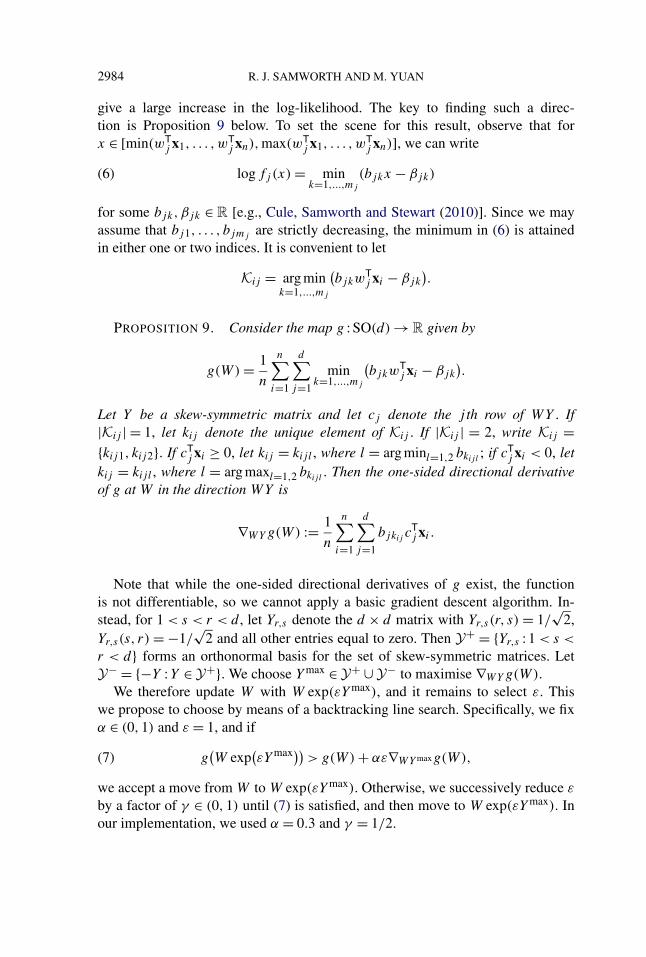
2984 R. J. SAMWORTH AND M. YUAN
give a large increase in the log-likelihood. The key to finding such a direc-tion is Proposition 9 below. To set the scene for this result, observe that forx ∈ [min(wT
j x1, . . . ,wTj xn),max(wT
j x1, . . . ,wTj xn)], we can write
logfj (x) = mink=1,...,mj
(bjkx − βjk)(6)
for some bjk, βjk ∈ R [e.g., Cule, Samworth and Stewart (2010)]. Since we mayassume that bj1, . . . , bjmj
are strictly decreasing, the minimum in (6) is attainedin either one or two indices. It is convenient to let
Kij = arg mink=1,...,mj
(bjkw
Tj xi − βjk
).
PROPOSITION 9. Consider the map g : SO(d) → R given by
g(W) = 1
n
n∑i=1
d∑j=1
mink=1,...,mj
(bjkw
Tj xi − βjk
).
Let Y be a skew-symmetric matrix and let cj denote the j th row of WY . If|Kij | = 1, let kij denote the unique element of Kij . If |Kij | = 2, write Kij ={kij1, kij2}. If cT
j xi ≥ 0, let kij = kij l , where l = arg minl=1,2 bkijl; if cT
j xi < 0, letkij = kij l , where l = arg maxl=1,2 bkijl
. Then the one-sided directional derivativeof g at W in the direction WY is
∇WY g(W) := 1
n
n∑i=1
d∑j=1
bjkijcTj xi .
Note that while the one-sided directional derivatives of g exist, the functionis not differentiable, so we cannot apply a basic gradient descent algorithm. In-stead, for 1 < s < r < d , let Yr,s denote the d × d matrix with Yr,s(r, s) = 1/
√2,
Yr,s(s, r) = −1/√
2 and all other entries equal to zero. Then Y + = {Yr,s : 1 < s <
r < d} forms an orthonormal basis for the set of skew-symmetric matrices. LetY − = {−Y :Y ∈ Y +}. We choose Y max ∈ Y + ∪ Y − to maximise ∇WY g(W).
We therefore update W with W exp(εY max), and it remains to select ε. Thiswe propose to choose by means of a backtracking line search. Specifically, we fixα ∈ (0,1) and ε = 1, and if
g(W exp
(εY max))
> g(W) + αε∇WY maxg(W),(7)
we accept a move from W to W exp(εY max). Otherwise, we successively reduce ε
by a factor of γ ∈ (0,1) until (7) is satisfied, and then move to W exp(εY max). Inour implementation, we used α = 0.3 and γ = 1/2.

ICA VIA NONPARAMETRIC MAXIMUM LIKELIHOOD 2985
Our algorithm produces a sequence (W(1), f(1)1 , . . . , f
(1)d ), (W(2), f
(2)1 , . . . ,
f(2)d ), . . . . We terminate the algorithm once
�n(W(t), f(t)1 , . . . , f
(t)d ) − �n(W(t−1), f
(t−1)1 , . . . , f
(t−1)d )
|�n(W(t−1), f(t−1)1 , . . . , f
(t−1)d )| < η,
where, in our implementation, we chose η = 10−7. As with other ICA algorithms,global convergence is not guaranteed, so we used 10 random starting points andtook the solution with the highest log-likelihood.
4. Numerical experiments. To illustrate the practical merits of our proposednonparametric maximum likelihood estimation method for ICA models, we con-ducted several sets of numerical experiments. To fix ideas, we focus on two-dimensional signals, that is, d = 2. The components of the signal were generatedindependently, and then rotated by π/3, so the mixing matrix is
A =(
1/2 −√3/2√
3/2 1/2
).
Our goal is to reconstruct the signal and estimate A or, equivalently, W = A−1,based on n = 200 observations of the rotated input.
We first consider a typical example in the ICA literature where the density ofeach component of the true signal is uniform on the interval [−0.5,0.5]. The topleft panel of Figure 1 plots the 200 simulated signal pairs, while the top right panelgives the rotated observations. The bottom left panel plots the recovered signalusing the proposed nonparametric maximum likelihood method. Also included inthe bottom right panel of the figure are the estimated marginal densities of the twosources of signal.
Figure 2 gives corresponding plots when the marginals have an Exp(1) − 1distribution. We note that both uniform and exponential distributions have log-concave densities and, therefore, our method not only recovers the mixing matrixbut also accurately estimates the marginal densities, as can be seen in Figures 1and 2.
To investigate the robustness of the proposed method when the marginal com-ponents do not have log-concave densities, we repeated the simulation in two othercases, with the true signal simulated first from a t-distribution with two degrees offreedom scaled by a factor of 1/
√2 and second from a mixture of normals dis-
tribution 0.7N(−0.9,1) + 0.3N(2.1,1). Figures 3 and 4 show that, in both cases,the misspecification of the marginals does not affect the recovery of the signal.Also, the estimated marginals represent estimates of the log-concave projection ofthe true marginals (a standard Laplace density in the case Figure 3), as correctlypredicted by our theoretical results.
As discussed before, one of the unique advantages of the proposed method overexisting ones is its general applicability. For example, the method can be used even

2986 R. J. SAMWORTH AND M. YUAN
FIG. 1. Uniform signal: top left panel, top right panel and bottom left panel give the true signal,rotated observations and the reconstructed signal, respectively. The bottom right panel gives theestimated marginal densities along with the true marginal (grey line).
when the marginal distributions of the true signal do not have densities. To demon-strate this property, we now consider simulating signals from a Bin(3,1/2) − 1.5distribution. To the best of our knowledge, none of the existing ICA methods areapplicable for these types of problems. The simulation results presented in Figure 5suggest that the method works very well in this case.
To further conduct a comparative study, we repeated each of the previoussimulations 200 times and computed our estimate along with those producedby FastICA and ProDenICA methods. FastICA algorithms [e.g., Hyvärinen andOja (2000), Nordhausen et al. (2011), Ollila (2010)] are popular ICA methodsthat traditionally proceed by maximising an approximation to the negentropy;ProDenICA is a nonparametric ICA method proposed by Hastie and Tibshirani(2003b), and has been shown to enjoy the best performance among a large col-lection of existing ICA methods [Hastie, Tibshirani and Friedman (2009)]. Boththe FastICA and ProDenICA methods were implemented using the R packageProDenICA [Hastie and Tibshirani (2003a)]. In the former case, we used theGfunc=G1 option to the ProDenICA function, corresponding to cosh negen-tropy [Hyvärinen and Oja (2000)]; in the latter case, we used the Gfunc=GPois

ICA VIA NONPARAMETRIC MAXIMUM LIKELIHOOD 2987
FIG. 2. Exponential signal: top left panel, top right panel and bottom left panel give the true signal,rotated observations and the reconstructed signal, respectively. The bottom right panel gives theestimated marginal densities along with the true marginal (grey line).
option, which fits a tilted Gaussian density using a Poisson generalised addi-tive model. To compare the performance of these methods, we follow convention[Hyvärinen, Karhunen and Oja (2001)] and compute the Amari metric between thetrue unmixing matrix W and its estimates. The Amari metric between two d × d
matrices is defined as
ρ(A,B) = 1
2d
d∑i=1
( ∑dj=1 |Cij |
max1≤j≤d |Cij | − 1)
+ 1
2d
d∑j=1
( ∑di=1 |Cij |
max1≤i≤d |Cij | − 1),(8)
where C = (Cij )1≤i,j≤d = AB−1. Boxplots of the Amari metric for all three meth-ods are given in Figure 6.
It is clear that both our proposed method (LogConICA) and ProDenICA out-perform the FastICA method. For both uniform and exponential marginals, Log-ConICA improves upon ProDenICA, which might be expected since both distri-butions have log-concave densities. It is, however, interesting to note the robust-ness of LogConICA to misspecification of log-concavity, as it still outperformsProDenICA for t2 marginals, and remains competitive for the mixture of normal

2988 R. J. SAMWORTH AND M. YUAN
FIG. 3. t2 signal: top left panel, top right panel and bottom left panel give the true signal, rotatedobservations and the reconstructed signal, respectively. The bottom right panel gives the estimatedmarginal densities along with the true marginal (grey line).
marginals. The most significant advantage of the proposed method, however, isdisplayed when the marginals are binomial. Recall that ProDenICA, in commonwith other nonparametric methods, assumes that the log density is smooth. This as-sumption is not satisfied with the binomial distribution and, as a result, ProDenICAperforms rather poorly. In contrast, LogConICA works fairly well in this settingeven though the true marginal does not have a log-concave density with respectto the Lebesgue measure. All these observations confirm our earlier theoreticaldevelopment.
5. Proofs.
PROOF OF PROPOSITION 1. (1) Suppose that∫Rd ‖x‖dP (x) = ∞. Fix an
arbitrary f ∈ F ICAd , and find α > 0 and β ∈ R such that f (x) ≤ e−α‖x‖+β . Then∫
Rdlogf dP ≤ −α
∫Rd
‖x‖dP (x) + β = −∞.
Thus, L∗∗(P ) = −∞ and ψ∗∗(P ) = F ICAd .

ICA VIA NONPARAMETRIC MAXIMUM LIKELIHOOD 2989
FIG. 4. Mixture of normals signal: top left panel, top right panel and bottom left panel give the truesignal, rotated observations and the reconstructed signal, respectively. The bottom right panel givesthe estimated marginal densities along with the true marginal (grey line).
(2) Now suppose that∫Rd ‖x‖dP (x) < ∞, but P(H) = 1 for some hyper-
plane H = {x ∈ Rd :a�
1 x = α}, where a1 is a unit vector in Rd and α ∈ R. Find
a2, . . . , ad such that a1, . . . , ad is an orthonormal basis for Rd . Define the family
of density functions
fσ (x) = 1
2σe−|aT
1 x−α|/σd∏
j=2
e−|aT
j x|
2.
Then fσ ∈ F ICAd , and
∫Rd
logfσ (x) dP (x) = − log(σ ) − d log 2 −d∑
j=2
∫H
∣∣aTj x
∣∣dP (x)
≥ − log(σ ) − d log 2 −d∑
j=2
∫H
‖x‖dP (x) → ∞
as σ → 0.

2990 R. J. SAMWORTH AND M. YUAN
FIG. 5. Binomial signal: top left panel, top right panel and bottom left panel give the true signal,rotated observations and the reconstructed signal, respectively. The bottom right panel gives theestimated marginal densities.
(3) Now suppose that P ∈ Pd . Notice that the density f (x) = 2−d ∏dj=1 e−|xj |
belongs to F ICAd and satisfies
∫Rd
logf dP = −d∑
j=1
∫Rd
|xj |dP (x) − d log 2 > −∞.
Moreover,
supf ∈F ICA
d
∫Rd
logf dP ≤ supf ∈Fd
∫Rd
logf dP < ∞,
where the second inequality follows from the proof of Theorem 2.2 of Dümbgen,Samworth and Schuhmacher (2011). We may therefore take a sequence f 1, f 2,
. . . ∈ F ICAd such that ∫
Rdlogf n dP ↗ sup
f ∈F ICAd
∫Rd
logf dP.

ICA VIA NONPARAMETRIC MAXIMUM LIKELIHOOD 2991
FIG. 6. Comparison between LogConICA, FastICA and ProDenICA. The bottom right panel givesthe Amari distances of the LogConICA and ProDenICA methods for the exponential example shownin the top right plot, but with a rescaled y-axis.
Let csupp(P ) denote the convex support of P , that is, the intersection of allclosed, convex sets having P -measure 1. The hypothesis P ∈ Pd implies thatcsupp(P ) is d-dimensional [e.g., Dümbgen, Samworth and Schuhmacher (2011),Lemma 2.1]. Following the arguments in the proof of Theorem 2.2 of Dümbgen,

2992 R. J. SAMWORTH AND M. YUAN
Samworth and Schuhmacher (2011), there exist α > 0 and β ∈ R such thatsupn∈N f n(x) ≤ e−α‖x‖+β for all x ∈ R
d . Moreover, these arguments [see alsothe proof of Theorem 4 of Cule and Samworth (2010)] yield the existence ofa closed, convex set C ⊇ int(csupp(P )), a log-concave density f ∗∗ ∈ Fd with{x ∈ R
d :f ∗∗(x) > 0} = C and a subsequence (f nk ) such that
f ∗∗(x) = limk→∞f nk (x) for all x ∈ int(C) ∪ (
Rd \ C
).
Since the boundary of C has zero Lebesgue measure, we deduce from Fatou’slemma applied to the non-negative functions x �→ −α‖x‖ + β − logf nk (x) that∫
Rdlogf ∗∗ dP ≥ lim sup
k→∞
∫Rd
logf nk dP = supf ∈F ICA
d
∫Rd
logf dP.
It remains to show that f ∗∗ ∈ F ICAd . We can write
f nk (x) = ∣∣detWk∣∣ d∏j=1
f kj
((wk
j
)Tx),
where Wk ∈ W and f kj ∈ F1 for each k ∈ N and j = 1, . . . , d . Let Xk be a ran-
dom vector with density f nk ∈ F ICAd , and let X be a random vector with density
f ∗∗ ∈ Fd . We know that Xk d→ X as k → ∞, and that (wk1)
TXk, . . . , (wkd)TXk are
independent for each k. Let wkj = wk
j/‖wkj‖ and f k
j (x) = ‖wkj‖f k
j (‖wkj‖x). Then
we have
f nk (x) = ∣∣det W k∣∣ d∏j=1
f kj
((wk
j
)Tx),(9)
where the matrix W k has j th row wkj . Moreover, W k ∈ W and f k
1 , . . . , f kd ∈ F1, so
(9) provides an alternative, equivalent representation of the density f nk , in whicheach row of the unmixing matrix has unit Euclidean length. By reducing to a fur-ther subsequence if necessary, we may assume that for each j = 1, . . . , d , thereexists wj ∈ R
d such that wkj → wj as k → ∞. By Slutsky’s theorem, it then fol-
lows that ((wk
1)T
Xk, . . . ,(wk
d
)TXk) d→ (
wT1X, . . . , wT
dX).
Thus, for any t = (t1, . . . , td)T ∈ Rd ,
E(eitT(wT
1X,...,wTdX)) = lim
k→∞E(eitT((wk
1)TXk,...,(wkd )TXk))
= limk→∞
d∏j=1
E(eitj (wk
j )TXk ) =d∏
j=1
E(eitj wT
j X).

ICA VIA NONPARAMETRIC MAXIMUM LIKELIHOOD 2993
We conclude that wT1X, . . . , wT
dX are independent. Now, the fact that the supportof f ∗∗ is a d-dimensional convex set means that none of wT
1X, . . . , wTdX is almost
surely constant, and each of these random variables has a log-concave density, byTheorem 6 of Prékopa (1973). Finally, since ‖wj‖ = 1 for all j , we deduce furtherthat W = (w1, . . . , wd)T is non-singular. This shows that f ∗∗ ∈ F ICA
d , as required.�
PROOF OF THEOREM 2. Suppose that P ∈ P ICAd satisfies
P(B) =d∏
j=1
Pj
(wT
j B)
for some W ∈ W and P1, . . . ,Pd ∈ P1. Consider maximising∫Rd
logf (x) dP (x)
over f ∈ Fd . Letting s = Wx and f (s) = f (As), where A = W−1, we can equiv-alently maximise ∫
Rdlog f (s) d
(d⊗
j=1
Pj (sj )
)
over f ∈ Fd . But, by Theorem 4 of Chen and Samworth (2012), the unique so-lution to this maximisation problem is to choose f (s) = ∏d
j=1 f ∗j (sj ), where
f ∗j = ψ∗(Pj ). This shows that f ∗ := ψ∗(P ) can be written as
f ∗(x) = |detW |d∏
j=1
f ∗j
(wT
j x).
Since f ∗ ∈ F ICAd also, we deduce that f ∗ is also the unique maximiser of∫
Rd logf dP over f ∈ F ICAd , so ψ∗∗(P ) = ψ∗(P ). �
PROOF OF THEOREM 3. Suppose that P ∈ P ICAd . Let X ∼ P , so there exists
W ∈ W such that WX has independent components. Writing Pj for the marginaldistribution of wT
j X, note that P1, . . . ,Pd ∈ P1. By Theorem 2 and the identifi-ability result of Eriksson and Koivunen (2004), it therefore suffices to show thatPj ∈ P1 has a Gaussian density if and only if ψ∗(Pj ) is a Gaussian density. If Pj
has a Gaussian density f ∗j , then since f ∗
j is log-concave, we have f ∗j = ψ∗(Pj ).
Conversely, suppose that Pj does not have a Gaussian density. Since f ∗j = ψ∗(Pj )
satisfies∫ ∞−∞ x dPj (x) = ∫ ∞
−∞ xf ∗j (x) dx [Dümbgen, Samworth and Schuhmacher
(2011), Remark 2.3], we may assume without loss of generality that Pj and f ∗j
have mean zero. We consider maximising∫ ∞−∞
logf dPj

2994 R. J. SAMWORTH AND M. YUAN
over all mean zero Gaussian densities f . Writing φσ 2 for the mean zero Gaussiandensity with variance σ 2, we have∫ ∞
−∞logφσ 2 dPj = − 1
2σ 2
∫ ∞−∞
x2 dPj (x) − 1
2log
(2πσ 2)
.
This expression is maximised uniquely in σ 2 at σ 2∗ = ∫ ∞−∞ x2 dPj (x). But Chen
and Samworth (2012) show that the only way a distribution Pj and its log-concaveprojection ψ∗(Pj ) can have the same second moment is if Pj has a log-concavedensity, in which case Pj has density ψ∗(Pj ). We therefore conclude that the onlyway ψ∗(Pj ) can be a Gaussian density is if Pj has a Gaussian density, a contra-diction. �
PROOF OF PROPOSITION 4. The proof of this proposition is very similar tothe proof of Theorem 4.5 of Dümbgen, Samworth and Schuhmacher (2011), so weonly sketch the argument here. For each n ∈ N, let f n ∈ ψ∗∗(P n), and consider anarbitrary subsequence (f nk ). By reducing to a further subsequence if necessary,we may assume that L∗∗(P nk ) → λ ∈ [−∞,∞]. Observe that
λ ≥ limk→∞
∫Rd
log(2−de
−∑dj=1 |xj |)
dP nk (x)
= −d log 2 −d∑
j=1
∫Rd
|xj |dP (x) > −∞.
Arguments from convex analysis can be used to show that the sequence (f nk )
is uniformly bounded above, and lim infk∈N f nk (x0) > −∞ for all x0 ∈int(csupp(P )). From this it follows that there exist a > 0 and b ∈ R such thatsupk∈N supx∈Rd f nk (x) ≤ e−a‖x‖+b. Thus, by reducing to a further subsequence ifnecessary, we may assume there exists f ∗∗ ∈ Fd such that
lim supk→∞,x→x0
f nk (x) = f ∗∗(x0) for all x0 ∈ Rd \ ∂
{x ∈ R
d :f ∗∗(x) > 0},
(10)lim sup
k→∞,x→x0
f nk (x) ≤ f ∗∗(x0) for all x0 ∈ ∂{x ∈ R
d :f ∗∗(x) > 0}.
Note from this that
λ = limk→∞
∫Rd
logf nk dP nk ≤ −a
∫Rd
‖x‖dP (x) + b < ∞.
In fact, we can use the argument from the proof of Proposition 1 to deduce thatf ∗∗ ∈ F ICA
d . Skorokhod’s representation theorem and Fatou’s lemma can then beused to show that λ ≤ ∫
Rd logf ∗∗ dP ≤ L∗∗(P ).We can obtain the other bound λ ≥ L∗∗(P ) by taking any element of ψ∗∗(P ),
approximating it from above using Lipschitz continuous functions, as in the proofof Theorem 4.5 of Dümbgen, Samworth and Schuhmacher (2011), and using

ICA VIA NONPARAMETRIC MAXIMUM LIKELIHOOD 2995
monotone convergence. From these arguments, we conclude that L∗∗(P n) →L∗∗(P ) and f ∗∗ ∈ ψ∗∗(P ).
We can see from (10) that f nka.e.→ f ∗∗, so
∫Rd |f nk − f ∗∗| → 0, by Scheffé’s
theorem. Thus, given any f n ∈ ψ∗∗(P n) and any subsequence (f nk ), we can findf ∗∗ ∈ ψ∗∗(P ) and a further subsequence of (f nk ) which converges to f ∗∗ in totalvariation distance. This yields the second part of the proposition. �
PROOF OF THEOREM 5. The first part of the theorem is a special case ofProposition 4. Now suppose P ∈ P ICA
d is identifiable and is represented by W ∈ Wand P1, . . . ,Pd ∈ P1. Suppose without loss of generality that ‖wj‖ = 1 for allj = 1, . . . , d and let f ∗∗ = ψ∗∗(P ). Recall from Theorem 2 that if X has densityf ∗∗, then wT
j X has density f ∗j = ψ∗(Pj ).
Suppose for a contradiction that we can find ε > 0, integers 1 ≤ n1 < n2 < · · · ,
f k ∈ ψ∗∗(P nk ) and (Wk,f k1 , . . . , f k
d )ICA∼ f k such that
infk∈N
infεkj∈R\{0}
infπk∈�d
{∥∥(εkj
)−1wk
πk(j)−wj
∥∥+∫ ∞−∞
∣∣∣∣εkj
∣∣f kπk(j)
(εkj x
)−f ∗j (x)
∣∣dx
}≥ ε.
We can find a subsequence 1 ≤ k1 < k2 < · · · such that wkl
j /‖wkl
j ‖ → wj , say, asl → ∞, for all j = 1, . . . , d . The argument toward the end of the proof of case(3) of Proposition 1 shows that W can be used to represent the unmixing matrixof f ∗∗, so by the identifiability result of Eriksson and Koivunen (2004) and the factthat ‖wj‖ = 1, there exist ε1, . . . , εd ∈ {−1,1} and a permutation π of {1, . . . , d}such that εj wπ(j) = wj . Setting πn = π and εn
j = ε−1j ‖wn
πn(j)‖, we deduce that
(εkl
j
)−1w
kl
πkl (j)= εj
wkl
π(j)
‖wkl
π(j)‖→ wj
for j = 1, . . . , d . Now observe that if Xkl has density f kl , then by Slutsky’s the-
orem, (εkl
j )−1(wkl
πkl (j))TXkl
d→ wTj X. It therefore follows from Proposition 2(c) of
Cule and Samworth (2010) that∫ ∞−∞
∣∣∣∣εkl
j
∣∣f n
πkl (j)
(εkl
j x) − f ∗
j (x)∣∣dx → 0
for j = 1, . . . , d . This contradiction establishes that
supf n∈ψ∗∗(P n)
sup(Wn,f n
1 ,...,f nd )
ICA∼ f n
infπn∈�d
infεn
1 ,...,εnd∈R\{0}
{∥∥(εnj
)−1wn
πn(j) − wj
∥∥
+∫ ∞−∞
∣∣∣∣εnj
∣∣f nπn(j)
(εnj x
) − f ∗j (x)
∣∣dx
}(11)
→ 0

2996 R. J. SAMWORTH AND M. YUAN
for each j = 1, . . . , d .It remains to prove that for sufficiently large n, every f n ∈ ψ∗∗(P n) is identi-
fiable. Recall from the identifiability result of Eriksson and Koivunen (2004) andTheorem 3 that not more than one of f ∗
1 , . . . , f ∗d is Gaussian. Let φμ,σ 2(·) de-
note the univariate normal density with mean μ and variance σ 2. Let J denotethe index set of the non-Gaussian densities among f ∗
1 , . . . , f ∗d , so the cardinality
of J is at least d − 1, and consider, for each j ∈ J , the problem of minimisingg(μ,σ) = ∫ ∞
−∞ |φμ,σ 2 − f ∗j | over μ ∈ R and σ > 0. Observe that g is continu-
ous with g(μ,σ) < 2 for all μ and σ , that infμ∈R g(μ,σ) → 2 as σ → 0,∞ andinfσ>0 g(μ,σ) → 2 as |μ| → ∞. It follows that g attains its infimum, and thereexists η > 0 such that
infj∈J
infμ∈R
infσ>0
∫ ∞−∞
∣∣φμ,σ 2 − f ∗j
∣∣ ≥ η.(12)
Comparing (11) and (12), we see that, for sufficiently large n, whenever f n ∈ψ∗∗(P n) and (Wn,f n
1 , . . . , f nd )
ICA∼ f n, at most one of the densities f n1 , . . . , f n
d
can be Gaussian. It follows that when n is large, every f n ∈ ψ∗∗(P n) is identifi-able. �
PROOF OF PROPOSITION 6. It is well known that for fixed W ∈ W , the non-parametric likelihood L(·) defined in (4) is maximised by choosing
P Wj = 1
n
n∑i=1
δwTj xi
, j = 1, . . . , d.
For i = 1, . . . , n, W ∈ W and j = 1, . . . , d , let
nwj(i) = {
i ∈ {1, . . . , n} :wTj x
i= wT
j xi
}.
The binary relation i ∼ i if nwj(i) = nwj
(i) defines an equivalence relation on{1, . . . , n}, so we can let IW
j denote a set of indices obtained by choosing oneelement from each equivalence class. Then
L(W, P W
1 , . . . , P Wd
) =d∏
j=1
|nwj(1)||nwj
(2)| · · · |nwj(n)|
nn
=d∏
j=1
n−n∏
i∈IWj
∣∣nwj(i)
∣∣|nwj(i)|
.
Note that |nwj(i)| ≤ d , because otherwise there would exist a subset of x1, . . . ,xn
of cardinality at least d + 1 lying on a (d − 1)-dimensional hyperplane of the form{x ∈ R
d :wTj x = β}, for some β ∈ R, contradicting the hypothesis that x1, . . . ,xn
are in general position. In fact, we claim that∑
i∈IWj
(|nwj(i)|−1) ≤ d −1. Indeed,

ICA VIA NONPARAMETRIC MAXIMUM LIKELIHOOD 2997
suppose for a contradiction that this were not the case. Then, by reordering theobservations if necessary, we could find K ≤ |IW
j |, integers n1, . . . , nK ≥ 2 with
n1 +· · ·+nK ≥ d +K and β1, . . . , βK ∈ R such that wTj xi = βk for i = n1 +· · ·+
nk−1 + 1, . . . , n1 + · · · + nk and k = 1, . . . ,K . Now set yik = xi − xn1+···+nkfor
i = n1 + · · · + nk−1 + 1, . . . , n1 + · · · + nk − 1 and k = 1, . . . ,K . Note that thereat least d vectors {yik}, all of which are non-zero, and any subset of cardinalityd is linearly independent because x1, . . . ,xn are in general position. On the otherhand, wT
j yik = 0 for all i, k, which establishes our contradiction. Thus, the bestwe can hope for in aiming to maximise the likelihood is to be able to choose|nwj
(i0)| = d for some i0 ∈ IWj , and |nwj
(i)| = 1 for i ∈ IWj \ {i0}. It follows that
L(W, P W1 , . . . , P W
d ) ≤ (dd/nn)d .Moreover, for any choice J of distinct indices in {1, . . . , n}, if we construct the
matrix WJ ∈ W as described just before the statement of Proposition 6, then foreach j = 1, . . . , d and i ∈ J \ {j}, we have wT
j xi = 1TdX−1
(−j)xi = 1, so |nwj(i)| = d
for such i, and L(WJ , PWJ
1 , . . . , PWJ
d ) = (dd/nn)d . �
As a preliminary to the proof of Corollary 8, it is convenient to define somemore notation. Let F ICA
d,0 denote the set of f ∈ F ICAd that can be represented using
an orthogonal unmixing matrix. Let ψ∗∗0 : Pd → F ICA
d,0 denote the log-concave ICA
projection operator onto F ICAd,0 , so that
ψ∗∗0 (P ) = arg max
f ∈F ICAd,0
∫Rd
logf dP.
The projection operator ψ∗∗0 has many properties in common with ψ∗∗. Indeed,
the analogue of Proposition 1 is immediate (in fact, the proof is slightly simplerbecause all rows of unmixing matrices have unit length). Let P ICA
d,0 denote the set
of P ∈ P ICAd such that any X ∼ P ICA
d has identity covariance matrix. Then the ana-logue of Theorem 2 states that the restriction ψ∗∗
0 |P ICAd,0
coincides with ψ∗∗|P ICAd,0
.
This follows because if the distribution of X belongs to P ICAd,0 , so that X = AS,
where S has independent components, then there is no loss of generality in assum-ing each component of S has unit variance, and then I = Cov(X) = AAT. Thus,the unmixing matrix of P may be assumed to be orthogonal, and the result fol-lows from Theorem 2. Analogues of Theorem 3 and Proposition 4 for ψ∗∗
0 areimmediate.
The proof of Corollary 8 is based on an analogue of part of Theorem 5 for P ICAd,0 ,
which is stated below. Its proof is virtually identical to that of Theorem 5, and isomitted.

2998 R. J. SAMWORTH AND M. YUAN
PROPOSITION 10. Suppose that P ∈ P ICAd,0 is identifiable and that (W,P1, . . . ,
Pd)ICA∼ P with W ∈ O(d). If P 1,P 2, . . . ∈ Pd are such that d(P n,P ) → 0, then
supf n∈ψ∗∗
0 (P n)
sup(Wn,f n
1 ,...,f nd )
ICA∼ f n
infπn∈�d
infεn
1 ,...,εnd∈{−1,1}
{∥∥(εnj
)−1wn
πn(j) − wj
∥∥
+∫ ∞−∞
∣∣∣∣εnj
∣∣f nπn(j)
(εnj x
) − f ∗j (x)
∣∣dx
}
→ 0
for each j = 1, . . . , d , where f ∗j = ψ∗(Pj ). As a consequence, for sufficiently
large n, every f n ∈ ψ∗∗0 (P n) is identifiable.
Notice that the scaling factors here may be assumed to belong to {−1,1}, againbecause the rows of Wn and W have unit length.
PROOF OF COROLLARY 8. Let z1 = �−1/2x1, . . . , zn = �−1/2xn, and letP n,z denote their empirical distribution. Writing z = n−1 ∑n
i=1 zi and x =n−1 ∑n
i=1 xi , note that the covariance matrix corresponding to P n,z is
1
n
n∑i=1
(zi − z)(zi − z)T = 1
n
n∑i=1
�−1/2(xi − x)(xi − x)T�−1/2 = I.
Now P n,z ∈ Pd provided the convex hull of z1, . . . , zn is d-dimensional, whichoccurs with probability 1 for sufficiently large n. It follows by the analogue ofProposition 1 for ψ∗∗
0 that there then exists a maximiser (On, gn1 , . . . , gn
d ) of�n(O,g1, . . . , gd; z1, . . . , zn) over O ∈ O(d) and g1, . . . , gd ∈ F1.
Now let � = Cov(x1), and note that the distribution P 0,z of �−1/2x1 belongs to
P ICAd,0 . Suppose that (O0,P
0,z1 , . . . ,P
0,zd )
ICA∼ P 0,z, with O0 ∈ O(d). To show that
d(P n,z,P 0,z)a.s.→ 0, note first that∣∣∣∣
∫Rd
‖x‖d(P n,z − P 0,z)(x)
∣∣∣∣≤
∣∣∣∣∣1
n
n∑i=1
{∥∥�−1/2xi
∥∥ − ∥∥�−1/2xi
∥∥}∣∣∣∣∣ +∣∣∣∣∣1
n
n∑i=1
∥∥�−1/2xi
∥∥ − E∥∥�−1/2x1
∥∥∣∣∣∣∣≤ 1
n
n∑i=1
∥∥(�−1/2 − �−1/2)
xi
∥∥ +∣∣∣∣∣1
n
n∑i=1
∥∥�−1/2xi
∥∥ − E∥∥�−1/2x1
∥∥∣∣∣∣∣≤ |λ|max
(�−1/2 − �−1/2)1
n
n∑i=1
‖xi‖ +∣∣∣∣∣1
n
n∑i=1
∥∥�−1/2xi
∥∥ − E∥∥�−1/2x1
∥∥∣∣∣∣∣,

ICA VIA NONPARAMETRIC MAXIMUM LIKELIHOOD 2999
where |λ|max(�−1/2 −�−1/2) denotes the largest absolute value of the eigenvalues
of �−1/2 − �−1/2. Now |λ|max(�−1/2 − �−1/2)
a.s.→ 0, by the strong law of largenumbers and the continuous mapping theorem, while n−1 ∑n
i=1 ‖xi‖ a.s.→ E‖x1‖,also by the strong law. Another application of the strong law shows that the secondterm in the sum converges almost surely to zero. Moreover, if h : Rd → [−1,1] hasLipschitz constant at most 1, then∣∣∣∣
∫Rd
h d(P n,z − P 0,z)∣∣∣∣
≤∣∣∣∣∣1
n
n∑i=1
{h(�−1/2xi
) − h(�−1/2xi
)}∣∣∣∣∣+
∣∣∣∣∣1
n
n∑i=1
h(�−1/2xi
) − Eh(�−1/2x1
)∣∣∣∣∣≤ |λ|max
(�−1/2 − �−1/2)1
n
n∑i=1
‖xi‖
+∣∣∣∣∣1
n
n∑i=1
h(�−1/2xi
) − Eh(�−1/2x1
)∣∣∣∣∣a.s.→ 0.
This shows that d(P n,z,P 0,z)a.s.→ 0, so by Proposition 10, there exist πn ∈ �d and
εn1 , . . . , εn
d ∈ {−1,1} such that
∥∥(εnj
)−1onπn(j) − o0
j
∥∥ +∫ ∞−∞
∣∣∣∣εnj
∣∣gnπn(j)
(εnj x
) − g∗j (x)
∣∣dxa.s.→ 0
for each j = 1, . . . , d , where g∗j = ψ∗(P 0,z
j ). Now set ˆWn = On�−1/2 and ˆ
f nj =
gnj , and observe that (
ˆWn,
ˆf n
1, . . . ,ˆ
f nd) maximises �n(W,f1, . . . , fd;x1, . . . ,xn)
over W ∈ O(d)�−1/2 and f1, . . . , fd ∈ F1. Since (O0�−1/2,P0,z1 , . . . ,P
0,zd )
ICA∼P 0, there exist π ∈ �d and scaling factors ε1, . . . , εd ∈ R \ {0} such thato0j�
−1/2 = ε−1j w0
π(j) and P0,zj (Bj ) = P 0
π(j)(εjBj ) for all Bj ∈ B1. It follows that,
setting ˆπn = πn ◦ π−1 and ˆεnj = ε−1
π−1(j)εnπ−1(j)
, we have
( ˆεnj
)−1 ˆwnˆπn(j)
= ( ˆεnj
)−1on
ˆπn(j)�−1/2
= επ−1(j)
(εnπ−1(j)
)−1onπn(π−1(j))
�−1/2
a.s.→ επ−1(j)o0π−1(j)
�−1/2 = w0j

3000 R. J. SAMWORTH AND M. YUAN
for j = 1, . . . , d . Now,
f ∗π(j)(x) = ψ∗(
P 0π(j)
)(x) = ∣∣ε−1
j
∣∣g∗j
(ε−1j x
),
where the second equality follows by the affine equivariance of log-concave pro-jections [Dümbgen, Samworth and Schuhmacher (2011), Remark 2.4]. Thus,∫ ∞
−∞∣∣∣∣ ˆεn
j
∣∣ ˆf n
ˆπn(j)
( ˆεnj x
) − f ∗j (x)
∣∣dx
=∫ ∞−∞
∣∣∣∣εnπ−1(j)
ε−1π−1(j)
∣∣gnπn(π−1(j))
(εnπ−1(j)
επ−1(j)x)
− ∣∣ε−1π−1(j)
∣∣g∗π−1(j)
(ε−1π−1(j)
x)∣∣dx
=∫ ∞−∞
∣∣∣∣εnπ−1(j)
∣∣gnπn(π−1(j))
(εnπ−1(j)
y) − g∗
π−1(j)(y)
∣∣dya.s.→ 0
as required. �
PROOF OF PROPOSITION 9. For ε > 0, let Wε = W exp(εY ), and let wj,ε
denote the j th row of Wε . Notice that
wTj,εxi = wT
j xi + εcTj xi + O
(ε2)
as ε ↘ 0. It follows that for sufficiently small ε > 0,
g(Wε) − g(W)
ε= 1
ε
n∑i=1
d∑j=1
{min
k=1,...,mj
(bjkw
Tj,εxi − βjk
)
− mink=1,...,mj
(bjkw
Tj xi − βjk
)}
= 1
ε
n∑i=1
d∑j=1
bjkij
(wT
j,εxi − wTj xi
)
→n∑
i=1
d∑j=1
bjkijcTj xi
as ε ↘ 0. �
Acknowledgements. We are very grateful to the Associate Editor and threeanonymous referees for their helpful comments and suggestions.
REFERENCES
BACH, F. R. and JORDAN, M. I. (2002). Kernel independent component analysis. J. Mach. Learn.Res. 3 1–48. MR1966051

ICA VIA NONPARAMETRIC MAXIMUM LIKELIHOOD 3001
CHEN, A. and BICKEL, P. J. (2005). Consistent independent component analysis and prewhitening.IEEE Trans. Signal Process. 53 3625–3632. MR2239886
CHEN, A. and BICKEL, P. J. (2006). Efficient independent component analysis. Ann. Statist. 342825–2855. MR2329469
CHEN, Y. and SAMWORTH, R. J. (2012). Smoothed log-concave maximum likelihood estimationwith applications. Statist. Sinica. To appear.
COMON, P. (1994). Independent component analysis, a new concept? Signal Proc. 36 287–314.CULE, M. and SAMWORTH, R. (2010). Theoretical properties of the log-concave maximum likeli-
hood estimator of a multidimensional density. Electron. J. Stat. 4 254–270. MR2645484CULE, M., SAMWORTH, R. and STEWART, M. (2010). Maximum likelihood estimation of a multi-
dimensional log-concave density. J. R. Stat. Soc. Ser. B Stat. Methodol. 72 545–607. MR2758237DÜMBGEN, L. and RUFIBACH, K. (2011). logcondens: Computations related to univariate log-
concave density estimation. J. Statist. Software 39 1–28.DÜMBGEN, L., SAMWORTH, R. and SCHUHMACHER, D. (2011). Approximation by log-concave
distributions, with applications to regression. Ann. Statist. 39 702–730. MR2816336ERIKSSON, J. and KOIVUNEN, V. (2004). Identifiability, separability and uniqueness of linear ICA
models. IEEE Signal Processing Letters 11 601–604.HASTIE, T. and TIBSHIRANI, R. (2003a). ProDenICA: Product density estimation for ICA using
tilted Gaussian density estimates R package version 1.0. Available at http://cran.r-project.org/web/packages/ProDenICA/.
HASTIE, T. and TIBSHIRANI, R. (2003b). Independent component analysis through product densityestimation. In Advances in Neural Information Processing Systems 15 (S. Becker and K. Ober-mayer, eds.) 649–656. MIT Press, Cambridge, MA.
HASTIE, T., TIBSHIRANI, R. and FRIEDMAN, J. (2009). The Elements of Statistical Learning.Springer, New York.
HYVÄRINEN, A., KARHUNEN, J. and OJA, E. (2001). Independent Component Analysis. Wiley,New York.
HYVÄRINEN, A. and OJA, E. (2000). Independent component analysis: Algorithms and applica-tions. Neural Netw. 13 411–430.
ILMONEN, P., NEVALAINEN, J. and OJA, H. (2010). Characteristics of multivariate distributionsand the invariant coordinate system. Statist. Probab. Lett. 80 1844–1853. MR2734250
ILMONEN, P. and PAINDAVEINE, D. (2011). Semiparametrically efficient inference based on signedranks in symmetric independent component models. Ann. Statist. 39 2448–2476. MR2906874
KARVANEN, J. and KOIVUNEN, V. (2002). Blind separation methods based on Pearson system andits extensions. Signal Proc. 82 663–673.
NORDHAUSEN, K., OJA, H. and OLLILA, E. (2011). Multivariate models and the first four mo-ments. In Nonparametric Statistics and Mixture Models 267–287. World Sci. Publ., Hackensack,NJ. MR2838731
NORDHAUSEN, K., ILMONEN, P., MANDAL, A., OJA, H. and OLLILA, E. (2011). Deflation-based FastICA reloaded. In Proceedings of 19th European Signal Processing Conference 2011(EUSIPCO 2011) 1854–1858.
OJA, H., SIRKIÄ, S. and ERIKSSON, J. (2006). Scatter matrices and independent component analy-sis. Austrian J. Statist. 35 175–189.
OLLILA, E. (2010). The deflation-based FastICA estimator: Statistical analysis revisited. IEEETrans. Signal Process. 58 1527–1541. MR2758026
OLLILA, E., OJA, H. and KOIVUNEN, V. (2008). Complex-valued ICA based on a pair of general-ized covariance matrices. Comput. Statist. Data Anal. 52 3789–3805. MR2427381
OWEN, A. (1990). Empirical Likelihood. Chapman & Hall, London.PLUMBLEY, M. D. (2005). Geometrical methods for non-negative ICA: Manifolds, lie groups and
toral subalgebras. Neurocomputing 67 161–197.

3002 R. J. SAMWORTH AND M. YUAN
PRÉKOPA, A. (1973). On logarithmic concave measures and functions. Acta Sci. Math. (Szeged) 34335–343. MR0404557
RUFIBACH, K. and DÜMBGEN, L. (2006). logcondens: Estimate a log-concave probability den-sity from i.i.d. observations R package version 2.01. Available at http://cran.r-project.org/web/packages/logcondens/.
SAMAROV, A. and TSYBAKOV, A. (2004). Nonparametric independent component analysis.Bernoulli 10 565–582. MR2076063
STATISTICAL LABORATORY
UNIVERSITY OF CAMBRIDGE
WILBERFORCE ROAD
CAMBRIDGE
CB3 0WBUNITED KINGDOM
E-MAIL: [email protected]: http://www.statslab.cam.ac.uk/~rjs57
H. MILTON STEWART SCHOOL OF INDUSTRIAL
AND SYSTEMS ENGINEERING
GEORGIA INSTITUTE OF TECHNOLOGY
ATLANTA, GEORGIA 30332USAE-MAIL: [email protected]: http://www2.isye.gatech.edu/~myuan/