Incremental Kernel Null Space Discriminant Analysis for Novelty Detection

Juncheng Liu1, Zhouhui Lian1∗, Yi Wang2,3, Jianguo Xiao1

1Institute of Computer Science and Technology, Peking University, China2School of Software, Dalian University of Technology, China

3Key Laboratory for Ubiquitous Network and Service Software of Liaoning Province, China

Abstract

Novelty detection, which aims to determine whether a

given data belongs to any category of training data or not,

is considered to be an important and challenging problem

in areas of Pattern Recognition, Machine Learning, etc.

Recently, kernel null space method (KNDA) was reported

to have state-of-the-art performance in novelty detection.

However, KNDA is hard to scale up because of its high com-

putational cost. With the ever-increasing size of data, ac-

celerating the implementing speed of KNDA is desired and

critical. Moreover, it becomes incapable when there exist

successively injected data. To address these issues, we pro-

pose the Incremental Kernel Null Space based Discriminant

Analysis (IKNDA) algorithm. The key idea is to extract new

information brought by newly-added samples and integrate

it with the existing model by an efficient updating scheme.

Experiments conducted on two publicly-available datasets

demonstrate that the proposed IKNDA yields comparable

performance as the batch KNDA yet significantly reduces

the computational complexity, and our IKNDA based nov-

elty detection methods markedly outperform approaches us-

ing deep neural network (DNN) classifiers. This validates

the superiority of our IKNDA against the state of the art in

novelty detection for large-scale data.

1. Introduction

Novelty detection, which aims to identify new or un-

known data that a system has not been trained with and was

not previously aware of [17], is a fundamental and on-going

research problem in areas of Pattern Recognition, Machine

Learning, Computer Vision, etc [21]. The novelty detection

procedure can be regarded as a binary classification task

where the positive exemplars are available and the negative

ones are insufficient or absent. To be a good classification

system, the ability to differentiate between known and un-

known objects during testing is desired. Yet, the problem

∗Corresponding author. E-mail: lianzhouhui@pku.edu.cn

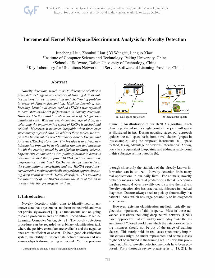
(a) Null space projections (b) Incremental update

Figure 1: An illustration of our IKNDA algorithm. Each

class is projected into a single point in the joint null space

as illustrated in (a). During updating stage, our approach

updates the null space basis from novel classes (grapes in

this example) using the proposed incremental null space

method, taking advantage of previous information. Adding

new class is equivalent to updating and adding a single point

in this subspace as illustrated in (b).

is tough since only the statistics of the already known in-

formation can be utilized. Novelty detection finds many

real applications in our daily lives. For animals, novelty

probably means a potential predator or a threat. Recogniz-

ing these unusual objects swiftly could survive themselves.

Novelty detection also has practical significance in medical

diagnoses. Doctors always need to pick up abnormality in a

patient’s index which has large possibility to be diagnosed

as a disease.

However, existing classification methods typically ne-

glect the importance of this property. Most of these ad-

vanced classifiers including deep neural network (DNN)

based approaches that are widely used today make the as-

sumption of “closed world”, in which the categories of test-

ing instances should not be out of the range of training

classes. This rarely holds in real cases since many impor-

tant classes might be under-represented and some classes

might not be included in the training set. To solve this prob-

lem, a number of novelty detection methods have been pro-

posed. For a thorough review please refer to [18, 21]. In

1792

2013, Bodesheim et al. [2] presented a novelty detection

method by leveraging the kernel null space based discrimi-

nant analysis which reports state-of-the-art performance on

two datasets. Their algorithm maps all instances within one

class to a single point in a joint null space, the novelty score

is obtained by simply calculating the shortest distance be-

tween the instance and the mapped classes. However, the

algorithm is hard to scale up because of the intensive com-

putation burden brought by the eigen-decomposition of the

kernel matrix. Additionally, their method cannot handle the

database where new data are injected successively, which

is a typical characteristic in novelty detection tasks. To ad-

dress these issues, we propose an incremental version of the

kernel null space discriminant analysis. Our algorithm is

able to handle incremental recognition tasks while signifi-

cantly reduces computing time without sacrificing detection

accuracy.

The rest of this paper is organized as follows: Section

2 reviews related work. Section 3 briefly describes the ba-

sic concepts of null space based LDA and its kernelization.

Then, our Incremental Kernel Null Space based Discrim-

inant Analysis (IKNDA) algorithm is presented with de-

tailed mathematical analyses in Section 4. Computational

complexity and storage requirement are analyzed in Sec-

tion 5. Section 6 presents experimental results, and Sec-

tion 7 concludes this paper by amplifying advantages of our

method and pointing out future work.

2. Related Work

As a subspace learning method, Linear Discriminant

Analysis (LDA) [14] and its variations have been studied for

many years. They have been widely applied in many appli-

cations of Pattern Recognition, Computer Vision, etc. such

as face recognition [5, 16], text-image combination multi-

media retrieval [19], speech and music classification [1],

outliers detection [22], generalized image and video clas-

sification [20, 24], and so on. A crucial step of these algo-

rithms lies in eigen-decomposition, which has a complex-

ity of O(N3). The computational time increases sharply

as the scale of training dataset enlarges. Using existing

approaches, during on-line updating process, new samples

are successively added to the existing training set, which

makes the batch computation quite inefficient. To solve

this problem, many efficient incremental algorithms have

been proposed [20, 9, 11, 27, 7]. Meanwhile, Kim et al.

applied the concept of sufficient spanning set approxima-

tion in each updating step [12]. Their algorithm reduced

the complexity to O(md2) where m and d denote the sam-

ple feature dimension and the reduced subspace dimension,

respectively. Sharma et al. proposed a fast implementa-

tion of null space LDA using random matrix multiplica-

tion [23]. However, these methods only consider the lin-

ear feature space, whereas kernel induced feature space is

more suitable for data with highly complex and non-linear

distributions [6]. Latter, Xiong et al. [25] proposed a QR

decomposition-based KDA algorithm in which QR decom-

position is applied rather than eigen-decomposition. How-

ever, it is hard to convert this algorithm to incremental learn-

ing mode, which hinders the further improvement of the

method’s performance. In 2007, a spectral regression-based

KDA method was presented by Cai et al. [4], it is shown that

their algorithm is 27 times faster than the ordinary KDA.

This paper proposes a new method that has even lower com-

putational cost and provides an intuitive way to conduct in-

cremental learning.

One major restriction when using LDA is the non-

singularity of within-class scatter matrix must be guaran-

teed, which is not always satisfied in practical situations. To

overcome this limitation, Yu et al. [26] and Huang et al. [10]

proposed the null space based method (KNDA) which takes

advantage of the null space [16]. The null space method

is suitable for the class-incremental process due to its in-

herent nature, i.e., each class is projected into one single

point in the null space where within-class scatter vanishes

and between-class scatter remains. Therefore, adding a new

class is equivalent to updating and adding a single point in

the subspace as illustrated in Figure 1.

Recently, Bodesheim et al. [2] reported that KNDA out-

performs other existing methods in novelty detection. How-

ever, as mentioned above, batch KNDA is hard to scale up

because of high computational cost and large storage re-

quirement, which limits the scenarios where KNDA can be

applied.

Developing an incremental method for kernel DAs is rel-

atively more difficult than linear DAs. In linear case, the

novel basis perpendicular to the space spanned by existing

centralized samples is expected to be relatively rare such

as [3]. However, in kernel induced feature space, the situa-

tion is quite different, i.e., the number of bases in this space

can be larger than the dimension of feature vectors, which

makes it impossible for these existing algorithms to work

properly.

In our IKNDA, new information is extracted from newly-

added samples and the proposed incremental null space is

employed. As we know, the null space based LDA typically

suffers from the over-fitting of training data, which how-

ever only has slight influence in our method compared to

the Kernel LDA. Furthermore, in contrast to other existing

methods, our approach takes advantage of a joint null space

(shown in Figure 1). Experimental results demonstrate that

the proposed IKNDA method yields performance similar

as that of the batch KNDA approach yet significantly re-

duces the computational complexity (more than 100 times

faster in some cases) in our experiments carried out on two

publicly-available datasets. By taking advantage of our pro-

posed algorithm, the kernel null space based LDA can be

793

Notation Descriptions

D Dimensionality of features

N Number of training data

X Existing data matrix

Y Newly-injected data matrix

Z Updated data matrix

B Orthogonal basis of zero-mean data

Π Centralizing operator by class-wise mean

H Centralizing operator by global mean

V Coefficients of XΦ for constructing B

β Null space of D

Xc,Yc,Zc Centralized data matrix

XΦ,YΦ,ZΦ Matrices in kernel induced feature space

µX ,µY ,µZ Mean vectors of X,Y and Z, respectively

K,K1,K2 Kernel matrices: XTΦXΦ,XT

ΦYΦ,YTΦYΦ

Table 1: Notations

more widely applied especially when handling large-scale

and incremental learning problems.

3. Mathematical Background

Given X = x1,x2, . . . ,xN ∈ RD×N , the main idea

is to minimize the within-class scatter and maximize the

between-class scatter simultaneously. Let Sb denote the

between-class scatter matrix and Sw denote the within-

class scatter matrix. LDA aims at finding a subspace basis

ϕ which maximizes the so-called fisher criterion as:

J(ϕ) =ϕTSbϕ

ϕTSwϕ. (1)

It is well known that the solution is given by solving a gen-

eralized eigenvalue problem:

Sbϕ = λSwϕ . (2)

The eigenvectors ϕ(1),ϕ(2), . . . ,ϕ(k) corresponding to klargest eigenvalues λ1, λ2, . . . , λk are collected as columns

of a transform matrix A and discriminative features of LDA

are computed by:

yi = ATxi, ∀i = 1, 2, . . . , N. (3)

The null space method is considered as a special case of

LDA when the within-class scatter in subspace vanishes and

the between-class scatter remains, which is also known as

Null Foley Sammon Transform(NFST) [8]:

ϕTSwϕ = 0ϕTSbϕ > 0 ,

(4)

and it is equivalent to:

ϕTStϕ > 0ϕTSwϕ = 0 ,

(5)

where St = Sb +Sw denotes the total scatter matrix. It can

be observed that the projections lie in the null space of Sw.

Let Nt and Nw be the null space of St and Sw, respectively,

and N⊥t ,N

⊥w denoting their orthogonal complements, we

have:

Nt = z ∈ RD|Stz = 0

Nw = z ∈ RD|Swz = 0 .(6)

It is easy to verify that the projection ϕ lies in the space:

ϕ ∈ N⊥

t ∩Nw . (7)

Then ϕ can be represented by a set of orthogonal bases B =b1,b2, . . . ,bn of N⊥

t as:

ϕ = Bβ . (8)

It has been proved [8] that N⊥t is exactly the space spanned

by zero-mean data x1 − µ,x2 − µ, . . . ,xN − µ with

µ = 1N

∑Ni=1 xi being the global mean vector. B can be

obtained by Gram-Schmidt ortho-normalization or standard

PCA [2]. By replacing ϕ with its basis expansion (8) , we

need to compute:

(BTSwB)β = 0 . (9)

The solution is null space of linear equations BTSwB

spanned by β(1),β(2), . . . ,β(C) with C being the number

of classes.

By rewriting Sw as XcXTc with Xc representing the

centralized data points corrected by the mean vector of

each corresponding class Xc = x1, x2, . . . , xN, xi =xi − µ(Ci) , ∀i = 1, 2, . . . , N , with Ci indicating the class

of sample i and µ(k) being the mean vector of class k, we

are able to reformulate (9) as:

DDTβ = 0 , (10)

where D = BTXc consists of the dot products of basis

vectors B and data points corrected by their mean vectors

of corresponding classes, which suggests the kernelization.

It should be pointed out that when training data is incre-

mented, both the orthogonal basis B and the within-class

scatter Sw are altered and should be calculated all over

again. Furthermore, the singular value decomposition of

new D is very time-consuming.

By taking advantage of previously obtained information,

the IKNDA algorithm proposed in this paper is able to up-

date D and its null space in an efficient way. In the follow-

ing section, both an incremental null space based LDA and

its kernelization will be presented.

4. Method Description

4.1. Incremental Null Space based LDA

For the purpose of incremental updating , we need to ex-

tract new information contained in newly-added data and

794

Figure 2: The new bases are perpendicular to the space

spanned by centralized existing data samples.

update the model by an efficient scheme. Assume X is

augmented by newly-added data set Y. We denote Z =X Y = x1,x2, . . . ,xN ,xN+1, . . . ,xN+l as the up-

dated sample points where X = x1, . . . ,xN represents

the existing samples and Y = xN+1, . . . ,xN+l the

newly-added points. Zc is the centralized data matrix cor-

rected by the mean vector of each class Zc = Xc,Yc.Thus, we have Zc = ZΠ,Π = I− L, where I is an iden-

tity matrix and L is a block diagonal matrix with block sizes

equal to the number of data points Nc in each class and the

value 1Nc

at each position [2]. Hl = Il −1l 1l1

Tl is a cen-

tralizing operator with 1l being an l-length all-one column

vector. YHl denotes the global mean-centralized new data

xN+1 − µY ,xN+2 − µY , . . . ,xN+l − µY . The mean

vectors of X and Y are, respectively, µX ,µY . With these

notations, the updated D can be formulated as follows:

(

BTXc BTYc

0 BTnewYc

)

, (11)

where Bnew1 is the new set of bases generated according

to newly-added data points which can be extracted from

Y =(

YHl

√

NlN+l (µX − µY )

)

. It consists of the

centralized newly-added samples and a mean shift vector as

well. The left bottom entry of (11) vanishes because the new

bases are perpendicular to the space spanned by centralized

existing data samples as illustrated by Figure 2, namely,

BTnewXc = 0. (12)

4.2. Integrating with Kernel Trick

A fundamental assumption of Null Space method is the

small sample size, i.e., N < D [2], which is often unsatis-

fied in practical cases. To overcome this shortcoming, the

kernel trick is frequently used, i.e., implicitly mapping the

sample points into a high-dimensional space, and perform-

ing null space in this Reproducing Kernel Hilbert Space

(RKHS). This procedure on the one hand effectively solves

1Note that Bnew consists of new bases generated by samples corrected

by global mean while Xc is the space spanned by samples corrected by the

mean vector of each corresponding class.

the problem mentioned above, on the other hand explores

the nonlinear structure of the data.

In the following, we use XΦ to denote as

the mapped sample points of existing samples

XΦ = Φ(x1),Φ(x2), . . . ,Φ(xN ), and YΦ to rep-

resent the mapped sample points of new samples

YΦ = Φ(xN+1),Φ(xN+2), . . . ,Φ(xN+l). Then,

we have ZΦ = XΦ YΦ. Similarly, the centralized

mapped data corrected by the corresponding mean vector

of each class are denoted by XcΦ and Yc

Φ. µXΦand µYΦ

are the mean vectors in high-dimensional space for XΦ and

YΦ. With these notations, YΦ can be derived as follows:

YΦ =(

YΦHl

√

NlN+l (µXΦ

− µYΦ))

(13)

= (XΦ YΦ)

(

0N ρ11N

Hl ρ21l

)

(14)

= (XΦ YΦ)

(

Ξ1

Ξ2

)

(15)

= ZΦΞ, (16)

where ρ1 =√

lN(N+l) , ρ2 = −

√

Nl(N+l) ,Ξ1 =

(

0N ρ11N

)

,Ξ2 =(

Hl ρ21l

)

, 0N denotes a N-

order square matrix of zeros, 1l is an l-length all-one col-

umn vector and similarly for 1N .

Equation (11) still holds in the kernel induced fea-

ture space. Since the vectors in this space have infi-

nite dimensions, B cannot be calculated explicitly. How-

ever, it can be reformulated as B = XΦV0, where

V0 = HQr(∆r)−1/2 is derived by the rank-r eigen-

decomposition of K as Qr∆r(Qr)T . Pairwise kernel dot

products in high-dimensional space are collected in kernel

matrix K, namely, K = XTΦXΦ. The kernel matrix is cen-

tralized as K = HKH. K is guaranteed to be positive-

definite by Reproducing Kernel Hilbert Theory. The first

entry in (11) for the kernel induced feature space can there-

fore be formulated as:

BTXcΦ = VT

0 XTΦXΦΠN (17)

= VT0 KΠN (18)

= D0. (19)

The right upper element of (11) can also be rewritten in

the same way:

BTYcΦ = VT

0 XTΦYΦΠl (20)

= VT0 K1Πl (21)

= D1, (22)

where K1 consists of the pairwise dot products between ex-

isting data XΦ and newly-added data YΦ.

795

The remaining problem is the calculation of Bnew, the

newly-introduced basis vectors that are perpendicular to the

space spanned by the existing mean-corrected data. Since

it cannot be calculated explicitly due to its infinite dimen-

sionality, here we employ again the kernel trick as described

in [6], and thus we can represent Bnew as ZΦVnew taking

advantage of the fact that Bnew can be represented by lin-

ear combinations of updated data ZΦ with Vnew being its

coefficients. We firstly introduce some extra matrices:

Γ = BT YΦ

Ψ = YΦ −BΓ,(23)

where Γ contains the projection coefficients of YΦ onto the

subspace spanned by B , while Ψ contains new information

in YΦ, which are normal to the aforementioned subspace:

Γ = BT YΦ = VT0 XΦ

TZΦΞ (24)

Ψ = YΦ −BΓ (25)

=(

XΦ YΦ

)

(

Ξ1 −V0Γ

Ξ2

)

(26)

= ZΦΩ . (27)

Instead of orthogonalizing Ψ directly to obtain Bnew,

we perform eigen-decomposition on ΨTΨ to get a set of

equivalent bases by collecting rank-r eigenvectors as in [6]:

Bnew = ΨQΨ∆−1/2Ψ = ZΦVnew, (28)

where ΨTΨ = QΨ∆ΨQTΨ and Vnew = ΩQΨ∆

−1/2Ψ .

Therefore the last element in (11) can be rewritten as:

BTnewY

cΦ = VT

newZTΦYΦΠl (29)

= VTnewK2Πl (30)

= D2 . (31)

Note that K2 can be augmented from K1.

By using the kernel trick, equation (11) boils down to:

D =

(

D0 D1

0 D2

)

. (32)

Having the solutions β(1),β(2), . . . ,β(C−1), corre-

sponding projections can be calculated by:

ϕ(j) = Bβ(j) = ZΦ[V0 Vnew]β(j). (33)

Having the updated coefficients V = [V0 Vnew], we have:

ϕ(j) = ZΦVβ(j) . (34)

The projected point of x is:

x∗

j = ϕ(j)TΦ(x) = β(j)TVTZT

ΦΦ(x)

= β(j)TVTk∗ ∀j = 1, 2, . . . , C − 1,

(35)

(a) (b) (c)

Figure 3: An illustrative comparison of the batch KNDA

with our IKNDA algorithm. (a): Vk−1 in batch mode. (b):

Vk in batch mode. Left part in (c): Vk−1 in incremental

mode. Right part in (c): Vk in incremental mode. As we

can see, the batch method computes bases without taking

advantage of previously computed matrix Vk−1. While,

our approach extracts new bases Vnew from novel classes,

marked in red square, then integrates with previously ob-

tained information Vk−1 (marked in green square).

where k∗ stores the dot products between x and all the

other existing data points in RKHS. During the updating

process, only matrices V and β need to be updated. V can

be obtained by integrating new information extracted from

newly-added data and existing bases as illustrated in Fig-

ure 3. β is updated by invoking our proposed incremental

null space method, more details of the algorithm will be

discussed in the following section.

4.3. Incremental Null Space Updating

By (32) , it can be observed that the updated matrix D is

augmented by D1,D2 from the existing matrix D0. Note

that the null space of DDT is equivalent to the null space

of DT .

The problem can then be tackled by the proposed incre-

mental null space scheme. Let the null space of DT be β,

then the product of DT and β is computed as:

DTβ =

(

DT0 0

DT1 DT

2

)(

β1

β2

)

= 0 . (36)

From above we observe that β1 must lie in β0 which spans

the null space of DT0 , since DT

0 β1 = 0. Therefore β1 can

be represented by linear combinations of β0:

β1 = β0α . (37)

Then, (36) can be rewritten as:

(

DT1 β0 DT

2

)

(

α

β2

)

= 0

s.t. αTα+ βT2 β2 = I ,

(38)

which can be solved by employing linear equation solver or

eigen-decomposition of matrix(

DT1 β0 D2

)

. Having

α and β2, the β is updated as [(β0α)T (β2)T ]T .

796

Figure 4: Representative images, two characters in six dif-

ferent font styles, of the FounderType-200 dataset.

The null space problem is much smaller scaled

by our proposed scheme which has a complexity of

O(l2(c + b − 1)), where l is the incremental size, c is

the number of classes and b is the number of new bases,

compared with a complexity of O((N + l)3) for the batch

KNDA. Implementation details of our proposed algorithm

are described as follows.

Algorithm : Incremental Kernel Null Space based DA

Initial Stage :

1: Centralize the kernel matrix : K = HKH.

2: Obtain V0 = HQr(∆r)−1/2 by conducting eigen-

decomposition of K = Q∆QT .

3: Compute D0 = (V0)TKΠ.

4: Compute the null space β0 of matrix DT0 .

Updating Stage :

1: Compute D1 = V(k−1)TK1Πl.

2: Compute new basis coefficient matrix Vnew.

3: Compute D2 = VTnewK2Πl.

4: Update βk by the algorithm described in Section 3.3.

5: Update Vk by integrating new bases:

Vk = [Vk−1 Vnew].6: k← k+1.

5. Time and Space Complexity

We can observe from the description presented above,

main operations of our method are two parts: basic matrix

multiplication and eigen-decomposition. As we know, the

complexity of matrix product is typically O(mnp) for two

matrices A ∈ Rm×n and B ∈ Rn×p, while the complexity

of eigen-decomposition is O(n3) for a square matrix C ∈Rn×n.

Without losing generality, we assume that one novel

class is injected in each iteration. By denoting the num-

ber of existing bases and new bases as a = size(V, 2) and

b = size(Vnew, 2), respectively, i.e., the column of matrix

V and Vnew, we are able to analyze each step’s complexity

in Updating Stage. In step 1, only matrix multiplication

is involved, which has a complexity of O(al(l + N)). In

step 2, an eigen-decomposition is performed whose com-

plexity is O(l3). In step 3, to obtain D2, a matrix prod-

(a) The CNN feature space. (b) Joint null space.

Figure 5: Joint null space of 100 classes in the

FounderType-200 dataset. Each class in (a) is mapped to

a single point in (b) (visualized by t-SNE).

IKNDA KNDA SRKDA

time O(l3 + alN) O((l +N)3) O(N2(l/2 + c))space O(Nl) O((l +N)2) O(Nl)

Table 2: Asymptotic complexity of IKNDA and the batch

mode KNDA in terms of a, l, and N , where l is the incre-

mental size, N is the number of existing samples, c is the

number of classes and a is bounded by N .

uct is conducted, costing O(bl(N + 2l)). Step 4 uses

our proposed incremental null space algorithm and costs

O(l2(c + b − 1)), where c denotes the number of current

classes. In general, l is relatively much smaller than N(l ≪ N ) and b ≪ a. The complexity can be therefore re-

duced to O(l3+alN), in which the time cost of implement-

ing eigen-decomposition is O(l3), and the total time spent

to implement matrix product is O(alN). Compared with

the complexity of O((l+N)3) for eigen-decomposition of

the batch KNDA method, the proposed approach is clearly

more efficient.

6. Experiments

6.1. Experimental Setups

In this section, we carry out experiments to evaluate the

performance of novelty detection methods on the follow-

ing two publicly-available datasets: FounderType-2002 and

Caltech-2563. The FounderType-200 dataset we built con-

sists of 200 different fonts produced by a company named

FounderType with each font containing 6763 Chinese char-

acter images. Examples of this dataset are shown in Fig-

ure 4. Caltech-256 is composed of 256 categories with un-

equal member sizes ranging from 80-800.

For FounderType-200, we randomly pick 100 fonts as

the novel class, namely, these samples will not be used

2http://www.icst.pku.edu.cn/zlian/IKNLDA/3http://www.vision.caltech.edu/Image_Datasets/

Caltech256/

797

in training. While the remaining is split into training and

test sets with equal size. Then we train a CNN network

(i.e., Alexnet [13]) for feature extraction. Note that only

the training set is utilized in the CNN training process. Af-

ter training the CNN, all the samples are feed-forward and

the output of the 7th fully connected layer is taken as fea-

tures (4096 dims). For Caltech-256 dataset we pick 128 cat-

egorizes as the novel class and the rest is split into training

and test sets in the similar way. For both datasets, the Radial

Basis Function (RBF) is adopted for kernel construction.

To simulate the on-line updating process, we incremen-

tally inject one class in every iteration. To perform novelty

detection, we first map the test sample x to the null space

as a single point x∗, and the corresponding novelty score

is calculated as the smallest distance (Euclidean distance)

between the point and all training class centers.

6.2. Results and Discussions

The learned CNN features of images in the

FounderType-200 dataset are visualized in Figure 5a,

from which we can see that large variance exists between

samples within the same class. While in the joint null space

(see Figure 5b), the variance vanishes for the same class,

i.e., each class is mapped into one single point in this space.

The probability of a given sample belonging to a known

class can be simply measured by the distance between the

sample and the mapped point of the class. This results in

a more effective novelty score compared to the original

feature space which explains the better performance (see

Figure 6,7) of the proposed IKNDA compared to the

method using a DNN classifier (i.e., Alexnet).

Figure 6 and Figure 7 plot the receiver operating char-

acteristic (ROC) curves of different methods evaluated on

FounderType-200 and Caltech-256 datasets, respectively.

We compare our method with batch-KNDA [15], Spec-

tral Regression KDA [4], DNN classifier and SVM in the

one-vs-rest framework. The proposed IKNDA yields a

ROC curve coincides exactly with the batch KNDA [15]

which validates the effectiveness of our algorithm. For the

FounderType-200 dataset, our method along with the batch

mode, achieve the best result following by the Spectral Re-

gression KDA [4] and DNN classifier. For the Caltech-

256 dataset, our method achieves similar results as other

methods compared here. Considering slighter difference

between images in the same character content but different

font styles, we believe that our method is more competitive

for novelty detection tasks on large-scale fine-grain data.

We can also observe from the performance comparisons

that our method along with other KDA approaches outper-

forms the DNN classifier in the original CNN feature space.

This suggests that the original CNN features is less capable

of handling novelty detection tasks without proper transfor-

mations. Through our experiments, we can see that the null

0 0.2 0.4 0.6 0.8 10

0.2

0.4

0.6

0.8

1

IKNDA

KNDA

SRKDA

DNN

SVM

Figure 6: ROC curves of five novelty detection methods

evaluated on the FounderType-200 dataset.

0 0.2 0.4 0.6 0.8 10

0.2

0.4

0.6

0.8

1

IKNDA

KNDA

SRKDA

DNN

SVM

Figure 7: ROC curves of five novelty detection methods

evaluated on the Caltech-256 dataset.

space based approach is well suited for this particular task.

As analyzed in section 5, the batch KNDA method shows

a cubic growth against data size in terms of time complex-

ity, while our proposed incremental algorithm is very ef-

ficient and mostly depends on the number of incremental

size. Comparisons of novelty detection accuracy (measured

by AUC values) are shown in Table 3 and 4. The AUC

values and computational times of 5 different methods are

listed in every iteration. In each iteration, we integrate 10

new classes into the existing model. It can be observed that

our method achieves a comparable performance compared

to the state of the art while significantly reduces the compu-

tational time. This validates the effectiveness and efficiency

of the proposed IKNDA algorithm in applications of nov-

elty detection for large-scale data. It should be pointed out

that, as shown in Table 2, the time complexity of IKNDA is

O(l3+alN) and O(N2(l/2+c) for SRKDA, where N and

l denote the training size and incremental size, respectively.

This means that the proposed IKNDA will also be much

more efficient than SRKDA when there exist large num-

bers of training samples but less incremental data, which

is commonly-seen in real applications.

Interestingly, we find that the AUC values of null space

798

AUC(%) training time(s)

#known Ours KNDA SRKDA SVM DNN Ours KNDA SRKDA SVM

10 95.91 95.91 93.81 81.99 65.63 0.13 2.87 0.09 8.90

20 93.86 93.86 94.02 67.54 67.74 0.44 16.72 0.38 28.21

30 92.14 92.14 93.52 63.70 72.46 0.95 49.54 0.90 68.45

40 92.23 92.23 93.27 58.92 74.32 1.58 104.55 1.49 138.51

50 88.98 88.98 91.80 61.85 74.85 2.41 196.07 2.51 234.18

60 86.46 86.46 90.34 60.90 75.53 3.38 327.22 3.72 366.61

70 86.32 86.32 88.63 60.34 75.96 4.56 499.37 5.64 494.54

80 86.12 86.12 88.87 60.30 75.68 4.16 781.96 8.01 634.69

90 85.82 85.82 88.30 57.58 73.69 5.40 1047.56 12.22 838.94

100 85.59 85.55 87.86 53.46 71.85 9.25 1335.06 12.77 886.10

Table 3: AUC values and training times of five novelty detection methods evaluated on the FounderType-200 dataset.

AUC(%) training time(s)

#known Ours KNDA SRKDA SVM DNN Ours KNDA SRKDA SVM

10 87.90 87.90 88.39 80.14 77.52 0.03 0.56 0.02 2.43

20 86.19 86.19 88.03 83.23 80.33 0.09 2.85 0.10 10.20

30 83.55 83.55 84.93 82.87 77.53 0.20 7.61 0.21 22.65

40 83.37 83.37 85.11 82.41 79.39 0.34 15.76 0.37 43.67

50 82.75 82.75 84.50 81.78 79.00 0.54 31.05 0.55 74.76

60 81.37 81.37 83.28 80.73 78.25 0.82 48.55 0.99 116.77

70 80.24 80.24 82.36 80.21 77.95 1.10 73.93 1.23 170.44

80 79.50 79.33 81.31 79.69 78.46 1.46 109.51 1.91 236.06

90 78.87 78.87 80.34 77.96 78.40 1.87 160.48 2.85 310.80

100 79.07 79.07 80.87 78.75 79.38 2.25 233.38 2.95 403.29

Table 4: AUC values and training times of five novelty detection methods evaluated on the Caltech-256 dataset.

based methods are slightly lower than KDA in some itera-

tions. This perhaps due to the fact that class variations are

eliminated in the extracted null space which leads to over-

fitting. Yet, as we can see from our experimental results, the

influence is slight.

7. Conclusion

This paper presented the incremental kernel null space

based discriminant analysis (IKNDA) algorithm. We first

briefly described the mathematical background of kernel

null space based linear discriminant analysis. Then we de-

duced the incremental form of the standard null space based

LDA. Finally, we proposed the IKNDA algorithm by in-

corporating the mathematical traits and an incremental null

space method. Experimental results showed that the pro-

posed algorithm obtains the performance that exactly coin-

cides with the batch mode method while significantly re-

duces the time complexity in terms of the magnitude of

order. The proposed method benefits from taking advan-

tage of the existing model and computing only new bases

brought by newly-added samples, then integrating them by

an efficient updating scheme. Computational advantages of

our method were proved theoretically as well as illustrated

experimentally.

Our method is well suited for handling novelty detec-

tion tasks on large-scale datasets that might be successively

injected and updated. Replacing batch computation with

our IKNDA can accelerate these applications significantly.

Furthermore, due to the incremental computations, our al-

gorithm is far more scalable than the batch method.

Our future work will concentrate on the compression of

samples as described in [6]. Note that even though the pro-

posed algorithm sets us free from having to implementing

the batch mode computation, we still have to store all sam-

ples in processing. Unnecessary storage can be reduced by

leveraging the sample compression techniques.

ACKNOWLEDGMENTS

This work was supported by National Natural Science

Foundation of China (Grant No.: 61672043, 61472015,

61672056 and 61402072), Beijing Natural Science Foun-

dation (Grant No.: 4152022) and National Language Com-

mittee of China (Grant No.: ZDI135-9).

799

References

[1] E. Alexandre-Cortizo, M. Rosa-Zurera, and F. Lopez-

Ferreras. Application of fisher linear discriminant analy-

sis to speech/music classification. In Computer as a Tool,

2005. EUROCON 2005. The International Conference on,

volume 2, pages 1666–1669. IEEE, 2005.

[2] P. Bodesheim, A. Freytag, E. Rodner, M. Kemmler, and

J. Denzler. Kernel null space methods for novelty detection.

In Computer Vision and Pattern Recognition (CVPR), 2013

IEEE Conference on, pages 3374–3381. IEEE, 2013.

[3] M. Brand. Incremental singular value decomposition of un-

certain data with missing values. In Computer VisionECCV

2002, pages 707–720. Springer, 2002.

[4] D. Cai, X. He, and J. Han. Efficient kernel discriminant

analysis via spectral regression. In Data Mining, 2007.

ICDM 2007. Seventh IEEE International Conference on,

pages 427–432. IEEE, 2007.

[5] T.-J. Chin, K. Schindler, and D. Suter. Incremental kernel

svd for face recognition with image sets. In Automatic Face

and Gesture Recognition, 2006. FGR 2006. 7th International

Conference on, pages 461–466. IEEE, 2006.

[6] T.-J. Chin and D. Suter. Incremental kernel principal com-

ponent analysis. Image Processing, IEEE Transactions on,

16(6):1662–1674, 2007.

[7] Y. A. Ghassabeh, F. Rudzicz, and H. A. Moghaddam. Fast

incremental lda feature extraction. Pattern Recognition,

48(6):1999–2012, 2015.

[8] Y.-F. Guo, L. Wu, H. Lu, Z. Feng, and X. Xue. Null foley–

sammon transform. Pattern recognition, 39(11):2248–2251,

2006.

[9] K. Hiraoka, K.-i. Hidai, M. Hamahira, H. Mizoguchi,

T. Mishima, and S. Yoshizawa. Successive learning of lin-

ear discriminant analysis: Sanger-type algorithm. In Pattern

Recognition, 2000. Proceedings. 15th International Confer-

ence on, volume 2, pages 664–667. IEEE, 2000.

[10] R. Huang, Q. Liu, H. Lu, and S. Ma. Solving the small sam-

ple size problem of lda. In Pattern Recognition, 2002. Pro-

ceedings. 16th International Conference on, volume 3, pages

29–32. IEEE, 2002.

[11] E. A. K. James and S. Annadurai. Implementation of incre-

mental linear discriminant analysis using singular value de-

composition for face recognition. In Advanced Computing,

2009. ICAC 2009. First International Conference on, pages

172–175. IEEE, 2009.

[12] T.-K. Kim, K.-Y. K. Wong, B. Stenger, J. Kittler, and

R. Cipolla. Incremental linear discriminant analysis using

sufficient spanning set approximations. In Computer Vision

and Pattern Recognition, 2007. CVPR’07. IEEE Conference

on, pages 1–8. IEEE, 2007.

[13] A. Krizhevsky, I. Sutskever, and G. Hinton. Imagenet classi-

fication with deep convolutional neural networks. In Neural

information processing systems, pages 1097–1105, 2012.

[14] P. A. Lachenbruch. Discriminant analysis. Wiley Online

Library, 1975.

[15] Y. Lin, G. Gu, H. Liu, and J. Shen. Kernel null foley-

sammon transform. In Proceedings of the 2008 International

Conference on Computer Science and Software Engineering-

Volume 01, pages 981–984. IEEE Computer Society, 2008.

[16] W. Liu, Y. Wang, S. Z. Li, and T. Tan. Null space-based

kernel fisher discriminant analysis for face recognition. In

Automatic Face and Gesture Recognition, 2004. Proceed-

ings. Sixth IEEE International Conference on, pages 369–

374. IEEE, 2004.

[17] M. Markou and S. Singh. Novelty detection: a review part

1: statistical approaches. Signal processing, 83(12):2481–

2497, 2003.

[18] S. Marsland. Novelty detection in learning systems. Neural

Comp. Surveys, 2003.

[19] C. Moulin, C. Largeron, C. Ducottet, M. Gery, and C. Barat.

Fisher linear discriminant analysis for text-image combina-

tion in multimedia information retrieval. Pattern Recogni-

tion, 47(1):260–269, 2014.

[20] S. Pang, S. Ozawa, and N. Kasabov. Incremental linear dis-

criminant analysis for classification of data streams. Systems,

Man, and Cybernetics, Part B: Cybernetics, IEEE Transac-

tions on, 35(5):905–914, 2005.

[21] M. A. F. Pimentel, D. A. Clifton, C. Lei, and L. Tarassenko.

A review of novelty detection. Signal Processing,

99(6):215–249, 2014.

[22] V. Roth. Kernel fisher discriminants for outlier detection.

Neural computation, 18(4):942–960, 2006.

[23] A. Sharma and K. K. Paliwal. A new perspective to null

linear discriminant analysis method and its fast implementa-

tion using random matrix multiplication with scatter matri-

ces. Pattern Recognition, 45(6):2205–2213, 2012.

[24] N. Vaswani and R. Chellappa. Principal components null

space analysis for image and video classification. Image Pro-

cessing, IEEE Transactions on, 15(7):1816–1830, 2006.

[25] T. Xiong, J. Ye, Q. Li, R. Janardan, and V. Cherkassky. Ef-

ficient kernel discriminant analysis via qr decomposition. In

Advances in Neural Information Processing Systems, pages

1529–1536, 2004.

[26] H. Yu and J. Yang. A direct lda algorithm for high-

dimensional datawith application to face recognition. Pattern

recognition, 34(10):2067–2070, 2001.

[27] H. Zhao and P. C. Yuen. Incremental linear discriminant

analysis for face recognition. Systems, Man, and Cybernet-

ics, Part B: Cybernetics, IEEE Transactions on, 38(1):210–

221, 2008.

800