Increasing Supply Chain Robustness through Process Flexibility

and Inventory

David Simchi-Levi ∗ He Wang † Yehua Wei ‡

This Version: January 1, 2015

Abstract

We study a hybrid strategy that uses both process flexibility and inventory to mitigate risks

of plant disruption. In this setting, a firm allocates inventory before disruption while facing

demand uncertainties; demand is realized after disruption, and the firm schedules its production

using process flexibility to minimize lost sales. This interplay between process flexibility and

inventory is modeled as a two-stage robust optimization problem. We show that the robust

optimization model can be formulated as a linear program and solved efficiently. Using analytical

and numerical analysis, we study the impact of different process flexibility designs on the firm’s

inventory decisions. Our analysis reveals three important insights regarding the impact of

process flexibility on (i) total inventory level; (ii) freedom in inventory placement; and (iii)

inventory allocation strategy. In particular, we find that under designs with high degrees of

process flexibility, the firm allocates more inventory to low demand variability products and less

inventory to high demand variability products.

Keywords: supply chain risk mitigation strategies, process flexibility, inventory, robust opti-

mization

1 Introduction

Over the past decade, supply chain disruption has emerged as an important business challenge.

Indeed, as reported by Munich Re, the number of financially significant natural catastrophes

have been steadily going up over the last decades (Hedde 2014). For instance, the 2011 flood

in Thailand reduced Intel’s quarterly revenue target by $1 billion.1 Toyota’s production in

Japan, to give another example, declined 31.4% in the first six months after the 2011 Japanese

earthquake, as compared with its forecast.2

To safeguard against future disruptions, firms have been adopting various risk mitigation

strategies to improve resiliency of their supply chains. In this study, we focus on two risk

∗Engineering Systems Division, Department of Civil & Environmental Engineering, and the Operations ResearchCenter, Massachusetts Institute of Technology, dslevi@mit.edu†Operations Research Center, Massachusetts Institute of Technology, wanghe@mit.edu‡The Fuqua School of Business, Duke University, yehua.wei@duke.edu1Wall Street Journal, Intel Cuts Its Outlook, December 13, 2011.2Standard & Poor’s, December 31, 2011.

1

mitigation strategies: holding additional inventory and adding (process) flexibility. While it

is well documented that both strategies can improve supply chain resiliency, the performance

of a hybrid risk mitigation strategy that combines inventory and process flexibility is not well

understood. Therefore, in this study, we seek to answer the following two questions. Given

different levels of flexibility, (i) how much inventory is needed to achieve a required level of

resiliency, and (ii) how does one optimally allocate inventory to the various products?

Next, we briefly explain how process flexibility and inventory are used as risk mitigation

strategies.

1.1 Risk Mitigation Strategies

Risk mitigation inventory, also known as protective inventory, is the additional inventory that is

dedicated to supply chain disruption and hence is independent of lead time, the review policy or

the details of the inventory management policy used on a day-to-day basis. Holding inventory

beyond cycle stock and safety stock has been identified in a number of papers as an important

tool for dealing with supply chain disruption (see literature review in §1.3). Unfortunately, if

disruptions last a long period of time, the firm needs to hold a large amount of inventory and

hence pay high inventory costs (Tomlin and Wang 2011).

Process flexibility is defined as the “ability to build different types of products in the same

manufacturing plant or on the same production line at the same time” (Jordan and Graves

1995). For example, under full flexibility design, each plant is capable of producing all products;

while under dedicated design, each plant is capable of producing just a single product, see

Figure 1. With process flexibility, the firm is in a better position to match available capacity

with variable demand. Unfortunately, implementing full flexibility can be very expensive since

each plant needs to be capable of producing all products (Simchi-Levi 2010), and as a result,

partial flexibility designs are considered. Under such designs, each plant is capable of producing

just a few products.

Figure 1: Process Flexibility Designs

6

Dedicated 2-Chain Partial Flexibility Full Flexibility

Plant Product

Intuitively, in the wake of a plant disruption, process flexibility allows the firm to “route”

its excess capacity to the disrupted plants. However, while process flexibility can help the firm

to safeguard against disruption, it is only viable when the firm has plenty of excess capacity in

its plants. When plants are highly utilized, process flexibility is no longer an effective strategy

to mitigate the impact of disruptions.

In sum, both inventory and process flexibility have their limitations as disruption mitigation

strategies. This motivates us to consider a hybrid strategy which combines inventory and process

flexibility. In such hybrid strategy, inventory provides excess capacity during disruption, thus

2

improving the firm’s ability to reroute production using process flexibility; Vice versa, the

existence of process flexibility greatly reduces the amount of inventory required. The synergy

between inventory and process flexibility makes the hybrid strategy more compelling than either

of the two strategies individually.

1.2 Overview and Summary of Results

Robust Optimization Model for Inventory Allocation. In §2, we propose a two-

stage robust optimization problem to model the firm’s risk mitigation strategies. In the first

stage, given a process flexibility design, the firm optimizes its inventory levels for all products

to ensure that demand shortage does not exceed a certain level subject to plant disruptions.

Uncertainties in plant disruption and product demand are modeled using uncertainty sets, which

are chosen to approximate probabilistic settings. In the second stage, after disruption happens

and demands are realized, the firm uses both inventory and process flexibility to minimize

demand shortage. In particular, the firm may leverage its manufacturing flexibility and choose

a production schedule to minimize lost sales.

We show that the robust optimization problem can be reformulated as a linear programming

problem (§3). This linear program can be solved quickly for systems with a moderate number of

products. In special cases where demand and disruption uncertainty sets satisfy certain symmet-

ric properties, we give a closed-form characterization of the optimal inventory decision. Using

this characterization, we analyze a family of different flexibility designs and show the impact of

these designs on the firm’s inventory decisions (§4). In particular, we consider three aspects: (i)

total inventory level, (ii) freedom in inventory placement, and (iii) inventory allocation strategy.

Total Inventory Levels. In §4.1, we characterize the exact total inventory levels for a

family of flexibility designs known as the K-chains. Using this characterization, we observe

that while changing from a dedicated network to a 2-chain design provides a large portion of

benefit, there is also significant benefit achieved by increasing the degree of flexibility beyond

the 2-chain design, even when demand variability is relatively low. We also observe that the

minimum inventory level associated with full flexibility can be often achieved by having limited

degrees of flexibility.

Freedom of Inventory Placements. In §4.2, we show that for many process flexibility

designs, the optimal solution that minimizes total inventory is not unique. In other words,

flexibility provides the firm with freedom of placing inventory to mitigate disruption. For exam-

ple, our analysis shows that for many different flexibility designs, the firm may choose to hold

inventory for just a few products, instead of holding inventory for every product.

Inventory Allocation Strategy. In §4.3, we find that when the firm has a high degree of

flexibility, it may be optimal to hold more inventory for products with lower demand variability,

and to hold less inventory for products with higher demand variability. A similar result is

observed in stochastic settings where we specify probability distributions of plant disruption and

product demands (§5.3). This observation is in contrast with classical inventory management

theory, which states that higher demand variance implies that more inventory is needed in order

to achieve the same service level. Indeed, we show that classical theory remains true when the

3

firm has a low degree of flexibility. But when plants are highly flexible, it is more effective to

satisfy high variability demand using plant capacity, and hence more inventory is allocated to

low variability demand.

The three insights described above are mostly obtained for systems where the number of

plants is equal to the number of products. Although such settings are not typical to real world

systems, as Jordan and Graves (1995) argues, understanding these ideal settings provides insight

into realistic scenarios. Indeed, in §5.4 we consider an example where the number of plants is

different than the number of products. This example is based on a real dataset with 16 vehicle

models and 8 assembly plants at General Motors presented in Jordan and Graves (1995). Using

numerical experiments, we find that all three main insights are carries over to this example.

1.3 Related Literature

There is rich literature on supply chain risk mitigation using inventory management strategies.

Most of these papers (e.g., Meyer et al. 1979, Song and Zipkin 1996, Arreola-Risa and DeCroix

1998) assume a single product setting. More recently, researchers have also studied inventory

mitigation strategies under multi-period, multi-echelon settings (e.g., Bollapragada et al. 2004,

DeCroix 2013).

Academics have also considered hybrid strategies where firms use both dual sourcing and

inventory to mitigate risks (e.g., Gurler and Parlar 1997, Tomlin 2006). Our paper is related

to the multiple sourcing/inventory mitigation literature in the following sense: A supply chain

design where multiple plants are able to produce the same product can be viewed as a multiple

sourcing strategy. However, dual sourcing is mostly studied in a single product system, while

our model includes multiple sources of supply (plants) and multiple products.

Process flexibility is also referred to as “mix flexibility” or “product flexibility”. The study

of partial process flexibility started with the seminal work of Jordan and Graves (1995). In

their paper, Jordan and Graves propose the long chain (a.k.a. 2-chain) design, and empirically

observe that while in the long chain each plant is capable of producing just a few products, this

strategy has almost the same expected sales as that of full flexibility. More recently, there has

been a series of theoretical developments in explaining the effectiveness of long chain and sparse

flexibilities designs (e.g., Chou et al. 2010, 2011, Simchi-Levi and Wei 2012, Wang and Zhang

2013, Simchi-Levi and Wei 2014). In parallel, the academic community also investigated the

(optimal) mix between dedicated and fully flexible resources (e.g., Fine and Freund 1990, Bish

and Wang 2004, Tomlin and Wang 2005, Goyal and Netessine 2011), and the properties of more

general flexible resource selection problems (e.g., Bassamboo et al. 2010).

Of particular interest to us is the research that observed flexibility as an effective tool to safe-

guard against supply disruption. Tomlin and Wang (2005) considers a risk mitigation strategy

that uses a combination of mix-flexibility and dual sourcing. Tang and Tomlin (2008) suggests

process flexibility as one of the five types of flexibility strategies that can be used to mitigate sup-

ply chain disruptions. And finally, Sodhi and Tang (2012) lists flexible manufacturing processes

as one of the eleven robust supply chain strategies.

To the best of our knowledge, this paper is the first to consider a hybrid strategy combining

partial process flexibility and inventory as a way to mitigate against supply disruption in multi-

products systems. The hybrid strategy requires the firm to allocate inventory before disruption

(ex-ante), and to schedule its flexible production after disruption (ex-post). Finally, in our

4

model, the inventory allocation decisions are made to ensure that the demand shortage is always

lower than some threshold under a set of scenarios. This modeling feature is common in the

robust optimization literature (e.g., Ben-Tal et al. 2009, Bandi and Bertsimas 2012). Also, it is

similar in spirit to the model studied in Graves and Willems (2000), where the firm commits to

a certain service level under a range of uncertainties.

2 Model

We consider a firm that has M plants, denoted by Si for i = 1, . . . ,M , and produces N products,

denoted by Tj for j = 1, . . . , N . A plant can produce one or multiple products, and the flexibility

design specifies which products each plant can make. More formally, the flexibility design can

be represented as a bipartite network, where a link (Si, Tj) exists if and only if plant i is able

to produce product j. We refer to the set of such links as F . For a given flexibility design Fand a subset of product A ⊂ T1, . . . , TN, we define PF (A) = Si : (Si, Tj) ∈ F , Tj ∈ A as the

plants that can produce at least one of these products.

The plant capacities and product demands are uncertain quantities. The uncertainties in

plant capacities capture plant disruptions, while the uncertainties in product demands capture

the fluctuation of market demand. In addition to flexibility, the firm also uses inventory to

protect the supply chain. Such inventory is referred to as risk mitigation inventory, and sj is

used to denote the inventory of product j.

The firm faces a two-stage decision problem. In the first stage, given the existing flexibility

structure, the firm determines the level of risk mitigation inventory for each product before

disruption happens and before product demands are realized. In the second stage, the firm

observes realized product demands and available plant capacities after disruption, and adjusts

its production schedule to minimize demand shortage.

The interplay between risk mitigation inventory and flexibility is a key factor that we capture

in our model. Inventory and flexibility are closely related, because the firm’s demand shortage

in the second stage is determined by the inventory decision in first stage as well as its flexibility

design. Although we didn’t include flexibility as a decision variable, we are going to consider a

family of different flexibility designs and analyze how different designs change the firm’s inventory

decisions.

We first define the firm’s second stage problem of minimizing shortage in §2.1, and then

outline the complete two-stage problem in §2.2.

2.1 Shortage Function

After disruption happens, suppose that the firm observes available capacity c = (c1, c2, . . . , cM )

for each plant and realized demand d = (d1, d2, . . . , dN ) for each product. We define Π(F , s, c,d)

to be the minimum demand shortage, given flexibility design F , inventory vector (decision from

the first stage) s = (s1, s2, . . . , sN ), capacities c and demands d.

Let xij be the units of product j produced by plant i, and lj be the shortage of product j.

5

Π(F , s, c,d) is expressed as the following optimization problem.

Π(F , s, c,d) = min

N∑j=1

lj∑i: (Si,Tj)∈F

xij + lj ≥ dj − sj , ∀1 ≤ j ≤ N

∑j: (Si,Tj)∈F

xij ≤ ci, ∀1 ≤ i ≤M

lj , xij ≥ 0.

The first constraint is the definition of shortage or lost sales for each product. The second

constraint specifies that the sum of units produced at each plant cannot exceed its realized

capacity. Without loss of generality, we assume that any product consumes one unit of capacity,

otherwise we can re-scale the units for each product. Throughout the paper, Π(F , s, c,d) will

be referred to as the shortage function.

We develop two properties of Π(F , s, c,d) for later use.

Lemma 1. Π(F , s, c,d) is convex in s, c and d.

Lemma 2. The optimal value of Π(F , s, c,d) can be rewritten as

Π(F , s, c,d) = maxA⊂T1,...,TN

∑Tj∈A

(dj − sj)−∑

Si∈PF (A)

ci (1)

Lemma 2 provides us with a combinatorial expression for the shortage function. The expres-

sion is similar to a min-cut type formulation in the network flow context. This is because of the

formulation Π(F , s, c,d) can be viewed as a network flow problem (shown in Appendix A).

2.2 Robust Optimization Model for Inventory Decision

In the first stage, the firm faces the problem of minimizing total inventory while ensuring that

the shortage is at most δ. In what follows, δ is referred to as the shortage allowance. We

use Uc ⊂ RM+ to denote the capacity uncertainty set, and Ud ⊂ RN+ to denote the demand

uncertainty set. Let s = (s1, s2, . . . , sN ) be the vector of inventory for all products. The

optimization problem can be formulated as the following worst-case (WM) model:

Problem-WM: min

N∑j=1

sj (2)

s.t. Π(F , s, c,d) ≤ δ, ∀c ∈ Uc,d ∈ Ud (3)

sj ≥ 0,∀1 ≤ j ≤ N. (4)

The robust optimization approach that we take differs from many risk mitigation methods

proposed in literature, which require firms to identify probabilities of disruption events. We show

in the next subsection that the uncertainty sets can be chosen using the Central Limit Theorem

to mimic the behavior of stochastic uncertainties, and therefore, Problem-WM can be viewed as

an approximation of the stochastic model. To ensure the insights obtained from Problem-WM

6

is not restrictive to the worst-case modelling assumption, we use numerical experiments to show

that our insights are also valid for its stochastic counterpart (§5).

The main reason we study the worst-case model is because its computational and analytical

tractability. In §3, we show that worst-case model can be solved efficiently using a linear

program even when the elements in the uncertainty sets are infinite. In §4, we show that if the

uncertainty set satisfies a certain symmetric property, we can characterize the optimal solution

and thus provide analytical expression for the optimal inventory levels.

The worst-case model also provides several other advantages compared to its stochastic

counterpart. First, it is difficult and often impossible to accurately assess the probability of a

plant disruption, because disruption can occur from so many different sources, whether from

natural disaster, epidemics or factory fire (Simchi-Levi 2010). Because the inventory level can

be very sensitive to the probability of disruption, considering the worst-case scenario may offer

a more “robust” approach. Second, for small probability events such as plant disruptions,

managers might find it useful to understand the maximum possible shortage of demand under

wide range of scenarios. This understanding may lead them to better identify scenarios where

the supply chain is most vulnerable.

2.3 Choice of Uncertainty Sets

We propose a class of demand uncertainty sets that mimic the properties of stochastic demand

distributions. Suppose that the demand for each product j is denoted by some random variable

Dj with mean µj . For the worst-case model, we consider a class of demand uncertainty sets of

the form

Ud = d|N∑j=1

dj ≤N∑j=1

µj + γ,

N∑j=1

|dj − µj | ≤ β, |dj − µj | ≤ αj ,∀1 ≤ j ≤ N, (5)

with parameters γ, β and αj for 1 ≤ j ≤ N . The parameter γ limits the deviation of total

realized demand from the total expected demand; the parameter β limits the total absolute

(L1) deviation between the realized demand and the mean demand; and finally, the parameters

αj for 1 ≤ j ≤ N limit the deviation of each product’s realized demand from its mean. The

values of αj , β and γ can be determined using probabilistic guidelines such as the Central Limit

Theorem (CLT), see Bandi and Bertsimas (2012) for a more detailed discussion on this topic.

Appendix B gives an example showing how to select these parameters.

The capacity uncertainty sets are chosen to reflect possible plant disruptions. When the

likelihood of plant disruption is low and disruptions at plants are weakly correlated, the chance

of disruptions happening at more than one plant is relatively small. In this case, we may let the

capacity uncertainty set Uc to include every scenario where a single plant is disrupted.

Because we are more interested in the capacity uncertainties that arise from disruption, we

choose not to model the recurrent production variabilities which may cause a slight increase or

decrease to the plant capacities. However, these variabilities can be modelled by again applying

CLT-type of constraints, and the theoretical results we develop in the paper apply to capacity

uncertainty sets with CLT-type of constraints as well.

7

3 Computational Algorithm

In the formulation of Problem-WM, for each specific set of capacity and demand, (c, d),

Π(F , s, c,d) ≤ δ can be expanded into a set of linear constraints by introducing a set of auxiliary

variables xc,d, lc,d for each c and d (§2.1). Unfortunately, because the number of elements in Ucand Ud can be infinite, this would give us an LP with infinitely many constraints and variables.

If Uc and Ud are polyhedra sets, by convexity of Π(F , s, c,d) (Lemma 1), we just need to consider

the extreme points of Uc and Ud. However, although there are finitely many extreme points, if

we simply expand Π(·) using the formulation in §2.1, we would have an astronomical number of

variables and constraints even for a system with just a handful of plants and products.

To avoid having a huge number of constraints and variables, we apply Lemma (2) and rewrite

Problem-WM as follows.

Problem-WM: min

N∑j=1

sj (6)

s.t. max(c,d)∈Uc×Ud

∑Tj∈A

(dj − sj)−∑

Si∈PF (A)

ci

≤ δ, ∀A ⊂ T1, . . . , TN (7)

sj ≥ 0,∀1 ≤ j ≤ N. (8)

Given A ⊂ T1, . . . , TN, observe that the values of c and d that maximize the left-hand side

of Equation (7) are independent of decision variables s. Therefore, we can find (cA,dA) for

every possible A ⊂ T1, . . . , TN by solving 2N optimization problems, where N is the number

of products. If Uc and Ud are polyhedra, there are 2N LPs with moderate size. Then, we can

solve Problem-WM as an LP with 2N constraints, where each constraint is associated with a

sepecific (cA,dA).

Problem-WM: min

N∑j=1

sj (9)

∑Tj∈A

(dAj − sj)−∑

Si∈PF (A)

cAi ≤ δ, ∀A ⊂ T1, . . . , TN, (10)

sj ≥ 0,∀1 ≤ j ≤ N. (11)

In our computational experience, Problem-WM can be solved within seconds for N ≤ 20.

The computational advantage of the worst case model over the stochastic model is quite signif-

icant. Indeed, solving a stochastic model with Type 2 service-level constraint (defined in §5)

with 10 products and 10 plants takes more than 500 seconds with 10000 random samples from

the disruption and demand distributions.3 By contrast, solving Problem-WM for demand and

capacity polyhedron uncertainty sets constructed using the methods described in Section 2.3

takes less than 0.4 second, which is more than 1000 times faster. Finally, note that a stochastic

model with Type 1 service-level constraint (defined in Appendix C) is non convex and therefore

not even computationally tractable.

3The timing is based on Gurobi 6.0.0 LP solver with an Intel Xeon E5440 processor (8 core, 2.83 GHz).

8

4 Analysis for K-Chain Designs

In order to gain insight and intuition on the inventory allocation strategy as well as the level of

inventory required under different degrees of flexibility, in this section, we will study the setting

where M = N . To study different degrees of process flexibility, we consider a canonical family

of process flexibility designs known as the K-chain, where K is a strictly positive integer. A

K-chain design is where plant 1 produces product 1 to product K, plant 2 produces product 2

to product K + 1, and in general plant i produces products i, i + 1, . . . , i + K − 1. Note that

the K-chain design is defined in Hopp et al. (2004) as K-skill chaining, in the context of labor

cross-training.

In § 4.1 and § 4.2, we will assume that the system is symmetric. That is, for any demand

instance d ∈ Ud, every permutation of d is also in Ud. Respectively, for any capacity instance

c ∈ Uc, every permutation of c is in Uc For a fixed uncertainty set Uc (and Ud), we define the

quantitative measures Cmin(t) (and Dmax(t)) as follows.

Definition 1. Define Cmin(t) := minc∈Uc∑ti=1 ci, and Dmax(t) := maxd∈Ud

∑tj=1 dj.

Because Uc and Ud are symmetric, Cmin(t) is the minimum possible sum of t entries of any c

in Uc and Dmax(t) is the maximum possible sum of t entries of any d in Ud. Note that because

both Uc and Ud only contain non-negative vectors, both Cmin(t) and Dmax(t) are non-decreasing

with t. If Uc is convex and Ud is concave, then both Cmin(t) and Dmax(t) can be computed

efficiently by solving convex optimization problems. Moreover, when Ud is a symmetric linear

polytope with the form

Ud = d |N∑j=1

dj ≤ N + γ,

N∑j=1

|dj − 1| ≤ β, |dj − 1| ≤ α,∀1 ≤ j ≤ N,

then we can characterize Dmax(t). The characterization is discussed in Appendix B.

4.1 Total Inventory Required by K-chain

Lemma 3. Suppose for any inventory allocation s = (s1, s2, . . . , sN ), the rearranged allocation

σ(s) = (s2, s3 . . . , sN , s1) (stock s2 units of product 1, etc.) is feasible for the Problem-WM,

then the optimal inventory allocation can be achieved by allocating inventory equally across all

products.

The symmetry of K-chain designs certainly satisfies the condition in Lemma 3, so we can

assume the optimal inventory allocation has the property where sj = s for all product j. This

property turns out to be very important for our analysis for two reasons. First, by restricting

ourselves to study inventory allocations satisfying sj = s for all product j, we greatly simplifies

the original optimization problem to an optimization problem with just a single variable. Second,

if sj = s for all product j, then both the inventories and the uncertainties are symmetric and

this allows us to derive a simple condition for checking the feasibility of s in Problem-WM.

Next, we show that for integers 1 ≤ K ≤ N , if F is a K-chain, then we can obtain a

closed-form analytical expression for the optimal inventory level.

Proposition 1. Let F be a K-chain, for some integer K between 1 and N . Then s is an

9

optimal inventory allocation if sj = s∗ for all 1 ≤ j ≤ N where

s∗ = max max1≤t≤N−K

Dmax(t)− Cmin(t+K − 1)− δt

, maxN−k<t≤N

Dmax(t)− Cmin(N)− δt

, 0.

Next, we will apply this expression to specific uncertainty sets Uc and Ud to better understand

the impact of K-chains on the optimal inventory level. In this analysis, we seek understand

the sensitivity of the inventory level to different values of K and different degrees of demand

variability.

Example. Consider capacity uncertainty set

Uc = c|(c1, . . . , cN ) | ci′ = 0, for some 1 ≤ i′ ≤ N, ci = 1, ∀1 ≤ i 6= i′ ≤ N, (12)

and demand uncertainty set

Ud = d|N∑j=1

dj ≤ N + 2√Nσ,

N∑j=1

|dj − 1| ≤√

3σN

2+ σ√N, |dj − 1| ≤

√3σ, ∀j = 1 . . . N.

(13)

where σ is some parameter between 0 and 1√3. Recall from §2.3, the choice of Uc fits the

setting where plants are subject to low probability, independent disruptions. The choice of Udfits empirically with the setting where products have i.i.d. uniform distributions over the range

[1−√

3σ, 1+√

3σ], see Appendix B. We test varying values of σ to analyze how different degrees

of demand variability affect the inventory level in the K-chain flexibility design.

We perform a numerical study for N = 12. Using Appendix B and Proposition 1, we get

that for K = 1, the optimal inventory level for 1-chain is equal to

12 ·max1 +√

3σ − δ, 6√

3σ − (δ − 1)

6,

6√

3σ − 1− δ10

,4√

3σ + 1− δ12

, 0; (14)

for 2 ≤ K ≤ 6, the optimal inventory level for K-chain is equal to

12 ·max6√

3σ − (K − 2 + δ)

6,

6√

3σ − 1− δ10

,4√

3σ + 1− δ12

, 0; (15)

and finally, for 7 ≤ K ≤ 12, the optimal inventory level for K-chain is the same as that of full

flexibility, which can be expressed as

12 ·max6√

3σ − 1− δ10

,4√

3σ + 1− δ12

, 0. (16)

Therefore, we can compute the optimal inventory level for any K-chain with different δ and σ.

In Tables 1, 2 and 3, we output the optimal total inventory levels for 1-chain (dedicated design),

2-chain, 3-chain, 4-chain, 5-chain and 12-chain (full flexibility design) under different variations

and different shortage allowances. The following is a summary of the insights obtained from

these tables.

First, full flexibility is never required to achieve the optimal inventory level. Indeed, a 7-chain

(in a 12-products system) would always require the same amount of inventory as full flexibility,

see Equation (16). Moreover, in our numerical examples, the 5-chain design achieves the same

10

Table 1: Optimal Level of Total Inventories for K-chains with δ = 0.K=1 K=2 K=3 K=4 K=5 K=12

σ=0 12 1 1 1 1 1σ=0.1 14.08 2.08 1.69 1.69 1.69 1.69σ=0.2 16.16 4.16 2.39 2.39 2.39 2.39σ=0.3 18.24 6.24 4.24 3.08 3.08 3.08σ=0.4 20.32 8.31 6.31 4.31 3.79 3.79

Table 2: Optimal Level of Total Inventories for K-chains with δ = 0.6.K=1 K=2 K=3 K=4 K=5 K=12

σ=0 4.8 0.4 0.4 0.4 0.4 0.4σ=0.1 6.88 1.09 1.09 1.09 1.09 1.08σ=0.2 8.96 2.96 1.79 1.79 1.79 1.79σ=0.3 11.04 5.04 3.04 2.48 2.48 2.48σ=0.4 13.11 7.11 5.11 3.17 3.17 3.17

inventory level as full flexibility for all of the parameters we studied.

Second, while changing a dedicated design to a 2-chain design provides a large benefit, the

benefit achieved by changing from 2-chain to 3-chain is also significant. This holds even when

the demand variability is not high. For example, under medium level of variability (σ = 0.3)

and zero shortage allowance (δ = 0), changing from dedicated to the 2-chain design reduces

total inventory by 66%, while changing from the 2-chain to the 3-chain further reduces the total

inventory (compared to the inventory of dedicated design) by another 11%. This observation is

somewhat different from the insight described in the process literature when no plant disruption

is present. In that case, it has been consistently observed that almost all of the benefits are

obtained by changing from dedicated to the 2-chain design. One intuitive way to explain the

improvement achieved by a 3-chain design over a 2-chain is that while the 2-chain design is very

effective in satisfying uncertain demand, the disruption would break the chain. Therefore, a

disruption reduces 2-chain’s ability to satisfy uncertain demand. On the other hand, a 3-chain

design will still form a chain even if one plant is down.

4.2 Inventory Freedom in K-chain

In this section, we focus on the following question, is there freedom in selecting different inventory

allocations that satisfy the same shortage allowance? We answer this question in affirmative,

and characterize the range of all optimal inventory allocations under the K-chain flexibility

Table 3: Optimal Level of Total Inventories for K-chains with δ = 1.2.K=1 K=2 K=3 K=4 K=5 K=12

σ=0 0 0 0 0 0 0σ=0.1 1.68 0.49 0.49 0.49 0.49 0.49σ=0.2 3.76 1.76 1.19 1.19 1.19 1.19σ=0.3 5.84 3.84 1.88 1.88 1.88 1.88σ=0.4 7.91 5.91 3.91 2.57 2.57 2.57

11

designs.

Consider a case with very low demand variation. Intuitively, under full flexibility design, the

optimal total inventory level that solves Problem-WM is equal to Dmax(N)−Cmin(N)− δ, the

maximum possible total demand minus the minimum total capacity and the shortage allowance.

By Lemma 3, this implies that the optimal inventory placement at each product j is equal toDmax(N)−Cmin(N)−δ

N .

Next, we make an assumption on demand variability to ensure that this is indeed the optimal

inventory allocation.

Assumption 1. For any 1 ≤ j ≤ N , for any d ∈ Ud, we have dj ≥ Dmax(N)−Cmin(N)−δN .

With Assumption 1, for any d ∈ Ud, if the inventory placement at each product j is equal

to Dmax(N)−Cmin(N)−δN , then all of the inventories can be used to satisfy product demands.

Therefore, for any demand d, a fully flexible firm can always first spend all of the inventories

to satisfy some of the demand, and then use all of its fully flexible capacities to satisfy the

remaining demand. Because the total amount of inventory we have is Dmax(N)−Cmin(N)− δand it is always used, we will always have enough fully flexible capacities to ensure that the lost

sales is lower than the allowance.

To better understand how restrictive Assumption 1 is, let us consider the example where

the demand uncertainty set Ud is defined by Equation (13) of the previous subsection. In that

example, Assumption 1 is satisfied if σ ≤ 0.397.

Next, we propose a metric for measuring how much freedom exists in inventory allocation of

a flexibility design.

Definition 2. Assume Assumption 1 holds and fix a flexibility design F . We say F has degree

of freedom of at least u if any s that satisfies the equations

0 ≤ sj ≤ u,∀1 ≤ j ≤ N, (17)

and

N∑j=1

sj = Dmax(N)− Cmin(N)− δ, (18)

is an optimal inventory allocation. We also define FREE(F) to be the maximum possible u.

For a given F , if there does not exists an s satisfying Equations (17) and (18) for some u,

then we define FREE(F)= 0. Note that with Assumption 1, full flexibility design always has a

non-zero degree of freedom by selecting u = Dmax(N)−Cmin(N)−δN .

Clearly, the larger FREE(F), the more freedom F has in choosing its inventory allocation.

Consider the example where δ = 0, Uc satisfies Equation (12) and Ud satisfies Equation (13)

with σ = 0. If F is a K-chain for any K ≥ 2, then FREE(F) = 1. Because the optimal total

inventory level is equal to Dmax(N)− Cmin(N)− δ = 1, it means that we can place this 1 unit

of inventory at any product and obtain an optimal inventory allocation.

In the next proposition, we provide a set of conditions to check if the K-chain designs has a

degree of freedom of at least u.

Proposition 2. Assume Assumption 1 holds, and fix some u ≤ mind∈Ud d1. Then for K ≥ 2,

12

the K-chain design has a degree of freedom of at least u if and only if

Dmax(t)− Cmin(t+K − 1)− δ ≤ 0, ∀1 ≤ t ≤ N − n∗

(19)

Dmax(t)− Cmin(t+K − 1)−Dmax(N) + Cmin(N) + (N − t)u ≤ 0, ∀N − n∗ < t ≤ N −K,(20)

where n∗ = maxK, dDmax(N)−Cmin(N)−δ

u e.

Using Proposition 2, we can study the range of optimal inventory allocations under K-chain

designs, if the optimal inventory level of full flexibility is Dmax(N)− Cmin(N) + δ.

Example. Again, we consider the example from Section 4.1 with N = 12, Uc defined by

Equation (12) and Ud defined by Equation (13). It is easy to check that with Ud being defined by

Equation (13), FREE(F) cannot be greater than mind∈Ud d1. Therefore, we can use Proposition

2 to numerically compute the maximum degree of freedom, FREE(F), for any design F that is

a K-chain. In Figure 2, we plot the maximum degree of freedom for K-chains under different

demand variabilities for K = 2, 3, 4, 5 and 12. The shortage allowance parameter, δ, is picked

to equal to 0.6, which is equal to 5% of the total capacity.

We observe that when σ = 0.3, the total inventory level is roughly 2.5 and the maximum

degree of freedom of full flexibility is approximately 0.5. Therefore, there exists an optimal

inventory allocation that places inventories at only 5 out of the 12 products. This implies that

there exist a sparse optimal inventory allocation, i.e., placing inventories at just a few products.

More surprisingly, the same freedom is also achieved by the 5-chain design, and even the

4-chain design has a maximum degree of freedom of approximately 0.4. This implies that an

optimal inventory allocation for 4-chain need to hold inventory at any 7 of the 12 products.

Finally, observe that the inventory freedom of 2-chain decreases quickly with increasing demand

variabilities.

It is important to note that the freedom of inventory allocation depends crucially on the fact

that all products have the same unit holding costs. If some products have different unit holding

costs, then there may not be a large range of inventory freedom and in fact, the optimal inventory

allocation may be unique. Nevertheless, if a manufacturer has a high degree of flexibility, then

the manufacturer can move around its inventories among products that have comparable unit

costs without significantly increasing the total inventory cost or decreasing the supply chain

robustness.

4.3 Inventory Allocation Strategy

The symmetric setting in the previous subsections assume demands for all products are in the

same range. However, it is often the case that the firm has some products facing various degrees

of variability.

To understand how process flexibility affects inventory decisions when products have differ-

ent demand variabilities, we consider a stylized setting with 2N products with equal expected

demand. Products 1, 3, . . . , 2N − 1 have the same high level of variability; products 2, 4, . . . , 2N

have the same low level of variability. Therefore, we refer to products with odd labels as high

variability products, while products with even labels as low variability products.

13

Figure 2: Maximum Degree of Freedom for K-chains with K = 2, 3, 4, 5, 12 (with δ = 0.6).

0

0.1

0.2

0.3

0.4

0.5

0.6

0.7

0.8

0.9

1

0.05 0.1 0.15 0.2 0.25 0.3 0.35

Optim

al Inventory Freedo

m

Demand Variability

K=2 K=3 K=4 K=5 K=12

In the robust optimization setting, we can model higher variability using larger demand

uncertainty set, and lower demand variability using smaller demand uncertainty set. Based on

the discussion in §2.3 and Appendix B, we let σ1, σ2 be two parameters with σ1 > σ2, and

consider the following demand uncertainty set

Ud =

d |2N∑j=1

dj ≤ 2N + 2√

(σ21 + σ2

2)N,

2N∑j=1

|dj − 1| ≤√

3(σ1 + σ2)N +

√(σ2

1 + σ22)N

2,

|d2j−1 − 1| ≤√

3σ1, |d2j − 1| ≤√

3σ2,∀1 ≤ j ≤ N.

The first two constraints are motivated by central limit theorem (CLT) to bound total variability

among all products. The last two constraints bound the variability for each individual product.

Note that odd and even products have different variability.

Since the demand set Ud is symmetric for odd products and even products, respectively, we

can easily verify that there exists an optimal inventory decision such that every odd product has

the same inventory level s1, and every even product has the same inventory level s2. Using the

computational algorithm proposed in §3, we compute the optimal inventory level for a network

of 12 plants, 6 high variability products and 6 low demand variability products. We test two

pairs of parameters: (σ1 = 0.4, σ2 = 0.2), (σ1 = 0.5, σ2 = 0.3).

The result in Figure 3 shows an interesting effect: As one would expect, the firm holds more

inventory for high variability demand when the degree of flexibility is small. This is similar to

the classical newsvendor model, where more inventory is needed to achieve the same fill rate as

the demand variability increases. But surprisingly, when the firm has high degree of flexibility, it

is optimal to hold more inventory for products facing lower variability, and to hold less inventory

for products with higher variability. We refer to such phenomenon as the flipping effect, since

the inventory levels of two kinds of products flipped as degree of flexibility, K, increases.

14

Figure 3: Inventory under Asymmetric Demand in K-chains

The flipping effect can be explained by relating our analysis to Push and Pull strategies (see,

e.g., Simchi-Levi 2010). In a Pull strategy, the firm produces to order by applying capacity. In a

Push strategy, the firm produces to stock, and then satisfies demand from inventory. When there

is high degree of flexibility, high variability products are typically served using Pull (capacity)

while low variability products are served using Push (inventory), so most inventory is allocated

to the low variability products while less inventory is allocated to the high variability products.

When there is low degree of flexibility, capacity is not enough to match supply with demand for

high variability products, so more inventory is allocated to the high variability products.

Another observation is that the flipping effect increases when demand variabilities, σ1 and σ2,

both increase. Indeed, in Figure 5, the flipping effect is more significant when σ1 = 0.5, σ2 = 0.3

(right panel). To explain this, note that the total inventory increases when both σ1 and σ2

increase. However, as σ1 increases, it is more efficient to satisfy high variability demands with

capacity (pull) and less inventory. Therefore, higher percentage of inventory is allocated to low

variability products and the flipping effect becomes more significant.

The flipping effect also occurs in probabilistic settings where probability distributions of

plant disruption and product demands are specified. We show similar results using numerical

experiments in §5.3.

5 Numerical Examples for Stochastic Model

So far, we have mainly focused on a worst-case (robust optimization) model, because the robust

optimization model can be computed efficiently and yields analytical solutions for symmetric

uncertainty sets. However, as we showed in §2.3, there is a close connection between the stochas-

tic model and the worst-case model, because we choose a certain form of uncertainty set inspired

by the probabilistic model. In this subsection, we use numerical examples to verify that many

of our insights of the worst-case model also hold for the stochastic model.

Under the stochastic model, we consider the problem that minimizes the total inventory

while ensuring that the expected shortage is at most δ. The constraint on the expected shortage

is also known as the Type 2 service-level constraint in the supply chain literature. Let C and D

be vectors representing random capacities and demands, respectively, and let s = (s1, . . . , sN )

be the inventory decision variables for all products. Using the shortage function Π(F , s,C,D)

15

Figure 4: Total Inventory Required under Symmetric Demand in K-chains

defined in §2.1, the optimization problem is defined as follows

Problem-SM: min

N∑j=1

sj (21)

s.t. EC,D[Π(F , s,C,D)] ≤ δ, (22)

sj ≥ 0,∀1 ≤ j ≤ N. (23)

5.1 Total Inventory Level

Consider a network of 10 plants and 10 products. We assume all plants have one unit of capacity,

and each plant may be disrupted independently with probability p = 0.1. Each product has

demand uniformly distributed between 1 − α and 1 + α, where α represents the variability of

the demand. Demand distributions are independent for different products. The objective is to

determine inventory level of each product such that the expected shortage is no more than 0.2

(fill rate = 98%).

We restrict our attention to the K-chain designs introduced in §4. We sample 5000 times

from demand and capacity distributions, and solve a stochastic program with these samples to

determine the optimal inventory level.

In Figure 4, we plot the total inventory level for 2-chain, 3-chain and 10-chain (full flexibility)

under different demand variability α. The figure shows that adding flexibility to 2-chain design

significantly reduces the inventory. In particular, this is true even for low demand variability.

This observation is consistent with the insights from the robust model, see §4.1, Tables 1–3.

5.2 Inventory Placement Freedom

Using the robust model, we found in §4.2 that process flexibility not only reduces the total

inventory required, but also offers freedom in placing inventory among different products. We

show the same observation in the stochastic setting.

To quantify the firm’s freedom in placing inventory, we consider sparsity constraints, that is,

constraints specifying that the firm can only hold inventory for a few products. We then compare

16

Table 4: Total Inventory Increase under Sparsity ConstraintProducts 1..9 1,2,4,5,7,8,9 1,3,5,7,9 1,4,7 1,62-chain 3.16% 11.36% 25.43% Inf Inf3-chain 0.04% 0.10% 0.21% 0.62% 3.26%10-chain 0.00% 0.00% 0.00% 0.00% 1.61%

Figure 5: Inventory under Asymmetric Demand in K-chains

the total inventory with the sparsity constraints to the total inventory in the unconstrained case.

By symmetry, we know that placing inventory equally among all products is always an optimal

solution, so we expect the total inventory to increase under the sparsity constraints. If the

increase is small, then a sparse inventory solution is near optimal, which implies that the firm

has the freedom of placing inventory for only a few products.

We use the same setting as in the previous subsection, and fix demand variability parameter

α = 0.3 and shortage allowance δ = 0.2 (98% fill rate). The results are listed in Table 4. The

header row shows the subsets of products that the firm can hold inventory for. The percentage

numbers are the increase in total inventory compared with the unconstrained case where any

product can hold inventory. “Inf” means the problem is infeasible for the given placement

constraint. We find that the 10-chain design (full flexibility) has high degree of freedom: When

restricting to holding inventory for only two products, the total inventory increases by merely

1.61%. In addition, the 3-chain design has significantly higher degree of freedom than the 2-chain

design.

5.3 Inventory Allocation Strategy

Next, we consider a modified setting where demand distributions are not i.i.d. In particular, we

label products from 1 to 10, and assume that products with odd labels have demand uniformly

distributed between 1 − α and 1 + α, while products with even labels have demand uniformly

distributed between 1 − β and 1 + β, for some β < α. The objective is to determine inventory

levels of each product so as to achieve an expected fill rate of at least 98%.

We tested two sets of parameters: (α = 0.6, β = 0.2), (α = 0.3, β = 0.1). It is easily

verified that all products with lower variability (odd labels) have the same inventory level, and

all products with high variability (even labels) have the same inventory level. Figure 5 presents

the result for the stochastic model, and it is consistent with the result from the robust model:

the figure verifies the flipping effect we observed in §4.3.

17

Figure 6: Flexibility Design in the Asymmetric Example

1

2

3

4

5

6

7

8

A

P

O

N

M

L

K

C

B

J

I

H

G

F

E

D

380

230

250

230

240

230

230

240

320

150

270

110

220

110

120

80

140

160

60

35

140

40

35

30

180

EX. DEMANDCAPACITY BASE DESIGN

1

2

3

4

5

6

7

8

A

P

O

N

M

L

K

C

B

J

I

H

G

F

E

D

380

230

250

230

240

230

230

240

320

150

270

110

220

110

120

80

140

160

60

35

140

40

35

30

180

EX. DEMANDCAPACITY 2-CHAIN

5.4 Unbalanced System Example

Finally, we consider an unbalanced system example where the number of plants and products

are unequal (M 6= N). This example is based on a real dataset of 16 vehicle models and 8

assembly plants at General Motors presented in Jordan and Graves (1995). We use the same

plant capacities and expected product demands as in their paper, see the left chart of Figure 6.

We assume that product demands are normally distributed random variables truncated at two

standard deviations. Product A to F (compact cars) have high variability demands, with a

coefficient of variation equal to 0.5 prior to truncation; Product G to P (full-sized and luxury

cars) have low variability demand, with a coefficient of variation equal to 0.3 prior to truncation.

Each plant is assumed to be disrupted independently with probability 0.1. The expected fill

rate is assumed to be 95%. For simplicity, we assume demands are independent.

There is no clear definition of a K-chain when the number of plants and products are unequal.

Based on the “chaining” principle, Jordan and Graves (1995) proposed an ad hoc method to add

process flexibility to the base design. They first cluster the plants and products into six groups,

then add six links to connect six groups and create a “2-chain” design, see the right chart of

Figure 6. Following their method, we also create “3-chain” and “4-chain” designs by adding

six links at a time, see Figure 7. There are many ways to add six links to the initial design.

Our objective here is not to find the “optimal” designs, but to create a family of designs with

increasing degree of flexibility, and analyze how inventory decisions change within this family.

Table 5 shows the total inventory required for different designs, as well as the percentage of

inventory allocated to high variability products (Product A to F). The observation is consistent

with the findings from the balanced systems. While changing from a base design to a 2-chain

18

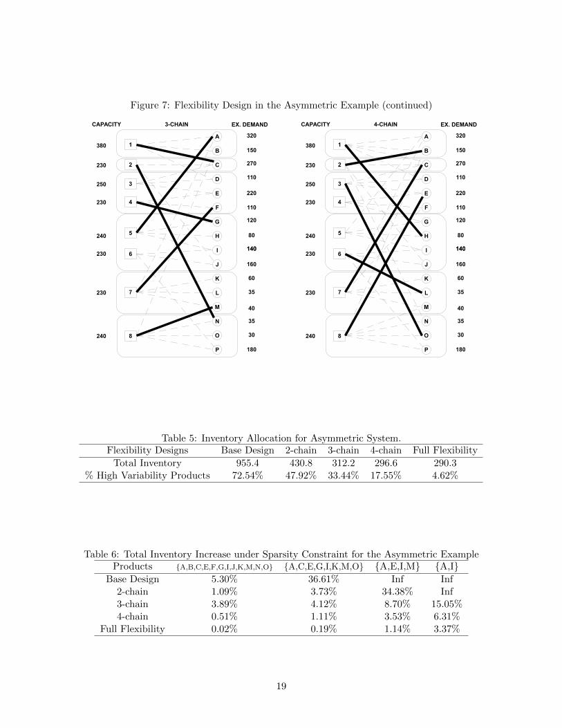
Figure 7: Flexibility Design in the Asymmetric Example (continued)

1

2

3

4

5

6

7

8

A

P

O

N

M

L

K

C

B

J

I

H

G

F

E

D

380

230

250

230

240

230

230

240

320

150

270

110

220

110

120

80

140

160

60

35

140

40

35

30

180

EX. DEMANDCAPACITY 3-CHAIN

1

2

3

4

5

6

7

8

A

P

O

N

M

L

K

C

B

J

I

H

G

F

E

D

380

230

250

230

240

230

230

240

320

150

270

110

220

110

120

80

140

160

60

35

140

40

35

30

180

EX. DEMANDCAPACITY 4-CHAIN

Table 5: Inventory Allocation for Asymmetric System.Flexibility Designs Base Design 2-chain 3-chain 4-chain Full Flexibility

Total Inventory 955.4 430.8 312.2 296.6 290.3% High Variability Products 72.54% 47.92% 33.44% 17.55% 4.62%

Table 6: Total Inventory Increase under Sparsity Constraint for the Asymmetric ExampleProducts A,B,C,E,F,G,I,J,K,M,N,O A,C,E,G,I,K,M,O A,E,I,M A,I

Base Design 5.30% 36.61% Inf Inf2-chain 1.09% 3.73% 34.38% Inf3-chain 3.89% 4.12% 8.70% 15.05%4-chain 0.51% 1.11% 3.53% 6.31%

Full Flexibility 0.02% 0.19% 1.14% 3.37%

19

design reduces total inventory, there is also significant inventory reduction from a 2-chain design

to higher degrees of flexibility. Moreover, as the degree of flexibility increases, less inventory is

allocated to high variability products.

We also consider sparsity constraints of inventory placement. Table 6 shows the increase of

total inventory compared with the unconstrained case where any product can hold inventory.

“Inf” means the problem is infeasible for the given placement constraint. Again, we find that

when there is high degree of flexibility, the firm can hold inventory for only a few products

without significantly increasing total inventory.

6 Time-to-Survive Model

In this section, we propose a supply chain risk metric called Time-to-Survive (TTS), and demon-

strate that it can be determined by solving a special case of our robust optimization model

introduced in §2.

Given a facility in the supply chain, e.g. a plant or a distribution center, the TTS is defined

as the longest time that customer service level is guaranteed if this facility is disrupted. The

TTS metric has been already implemented at Ford Motor Company to assess risk exposure

in its complex supply chain and evaluate Ford’s risk mitigation strategies (Simchi-Levi et al.

2014a,b).4

The definition of TTS is motivated by the concept of Time-to-Recover (TTR), which is the

time for a facility to return to full capacity after a disruption. TTR is widely used to evaluate

supply chain risk (see e.g. Hopp et al. 2012). If TTS is greater than TTR, then a disruption in

that facility is not going to affect the firm’s service level. On the other hand, when TTS for a

specific facility is shorter than TTR, than a disruption at that facility will have an impact on

service. Thus, an important challenge in supply chain risk management is to allocate inventory

to different products to increase the supply chain’s time to survive.

For this purpose, we define the supply chain TTS as the minimum (worst) TTS among all

its facilities. The longer the supply chain TTS, the more robust the supply chain is. Below we

show that the problem of allocating inventory to maximize supply chain TTS can be reduced

to a special case of the model in §2.

Suppose that plant i has capacity ci (i = 1, . . . ,M), product j has a constant demand rate

dj per unit time (j = 1, . . . , N). Let rj be the amount of inventory allocated to product j,

and assume that the sum of inventory among all products cannot exceed a given budget R. We

define a finite set Ω as the set of disruption scenarios, and let δ(ω)i be 0 if plant i is disrupted

in scenario ω ∈ Ω and 1 otherwise. We then formulate the problem of maximizing supply chain

4This work was awarded the 2014 INFORMS Daniel H. Wagner Prize for excellence in operations research practice.

20

TTS as the following nonlinear program:

TTS = maxrj ,x

(ω)ij

t

subject to t ≤ rj

dj −∑

i: (i,j)∈Fx(ω)ij

, ∀ 1 ≤ j ≤ N, ω ∈ Ω

∑j: (i,j)∈F

x(ω)ij ≤ ciδ

(ω)i , ∀ 1 ≤ i ≤M, ω ∈ Ω

N∑j=1

rj ≤ R, rj , x(ω)ij ≥ 0.

In this formulation, x(ω)ij denotes the production of product j by plant i in disruption scenario

ω. The first constraint is the definition of TTS: In any scenario, the supply chain must survive

the disruption by continuously supplying all products for at least t time units. The second

constraint requires that production does not exceed plant capacity. The last constraint specifies

that total inventory cannot exceed a given budget R.

Let sj = rj/t, we can rewrite the TTS model as

minsj ,x

(ω)ij ≥0

M∑j=1

sj

subject to dj −∑

i: (i,j)∈F

x(ω)ij ≤ sj , ∀ 1 ≤ j ≤ N, ω ∈ Ω

∑j: (i,j)∈F

x(ω)ij ≤ ciδ

(ω)i , ∀ 1 ≤ i ≤M, ω ∈ Ω.

This is a special case of the model in §2 where there is no demand uncertainty and the shortage

allowance equals to δ = 0.

7 Conclusion

We consider a firm using process flexibility and inventory to mitigate risk from plant disruptions,

with particular focus on the interplay between the two strategies. This interplay is modeled as

a two-stage robust optimization problem. In the first stage, given the firm’s process flexibility

design, the firm optimizes its inventory levels for all products in order to guarantee that demand

shortage never exceeds some constant, subject to plant disruptions. Uncertainties from plant

disruptions and product demands are modeled using uncertainty sets. In the second stage, after

disruption occurs, demands are realized, and the firm uses both inventory and process flexibility

to minimize demand shortage. In particular, the firm may leverage its process flexibility, and

reallocate production capacities to better match supply with demand.

We show that the robust optimization model can be solved efficiently by reformulating it

as a linear program. Moreover, we derive analytical results for a canonical family of flexibility

designs known as K-chain designs, and find the following managerial insights. First, while a

2-chain design is not as effective as K-chain designs for K > 2, full flexibility is often not

needed. Second, with high the degree of flexibility, the firm has freedom in placing inventory to

21

only a few products without affecting system performance. Finally, when the firm has a high

degree of flexibility, more inventory is allocated to products with low demand variability, and

less inventory is allocated to products with high demand variability. These insights are verified

by numerical experiments in a probabilistic setting for systems where the number of plants is

not necessarily equal to the number or products.

References

Arreola-Risa, A. and DeCroix, G. (1998). Inventory management under random supply disrup-

tions and partial backorders. Naval Research Logistics, 45(7):687–703.

Bandi, C. and Bertsimas, D. (2012). Tractable stochastic analysis in high dimensions via robust

optimization. Mathematical programming, 134(1):23–70.

Bassamboo, A., Randhawa, R. S., and Van Mieghem, J. A. (2010). Optimal flexibility configura-

tions in newsvendor networks: Going beyond chaining and pairing. Management Science,

56(8):1285–1303.

Ben-Tal, A., El Ghaoui, L., and Nemirovski, A. (2009). Robust optimization. Princeton Univer-

sity Press.

Bish, E. and Wang, Q. (2004). Optimal investment strategies for flexible resources, considering

pricing and correlated demands. Operations Research, 52(6):954–964.

Bollapragada, R., Rao, U. S., and Zhang, J. (2004). Managing inventory and supply performance

in assembly systems with random supply capacity and demand. Management Science,

50(12):1729–1743.

Chou, M., Teo, C.-P., and Zheng, H. (2011). Process flexibility revisited: The graph expander

and its applications. Operations Research, 59(5):1090–1105.

Chou, M. C., Chua, G. A., Teo, C.-P., and Zheng, H. (2010). Design for process flexibility:

Efficiency of the long chain and sparse structure. Operations Research, 58(1):43–58.

DeCroix, G. A. (2013). Inventory management for an assembly system subject to supply dis-

ruptions. Management Science, 59(9):2079–2092.

Fine, C. H. and Freund, R. M. (1990). Optimal investment in product-flexible manufacturing

capacity. Management Science, 36(4):449–466.

Goyal, M. and Netessine, S. (2011). Volume flexibility, product flexibility, or both: The role

of demand correlation and product substitution. Manufacturing & Service Operations

Management, 13(2):180–193.

Graves, S. C. and Willems, S. P. (2000). Optimizing strategic safety stock placement in supply

chains. Manufacturing & Service Operations Management, 2(1):68–83.

Gurler, U. and Parlar, M. (1997). An inventory problem with two randomly available suppliers.

Operations Research, 45(6):904–918.

Hedde, C. (2014). 2013 Natural Catastrophe Year in Review - US/Global Natural Catastrophe

Update. Webinar.

Hopp, W., Iravani, S., and Liu, Z. (2012). Mitigating the impact of disruptions in supply chains.

In Gurnani, H., Mehrotra, A., and Ray, S., editors, Supply Chain Disruptions, pages 21–49.

Springer London.

22

Hopp, W. J., Tekin, E., and Van Oyen, M. P. (2004). Benefits of skill chaining in serial production

lines with cross-trained workers. Management Science, 50(1):83–98.

Jordan, W. C. and Graves, S. C. (1995). Principles on the benefits of manufacturing process

flexibility. Management Science, 41(4):577–594.

Meyer, R. R., Rothkopf, M. H., and Smith, S. A. (1979). Reliability and inventory in a

production-storage system. Management Science, 25(8):799–807.

Simchi-Levi, D. (2010). Operations Rules: Delivering Customer Value through Flexible Opera-

tions. The MIT Press.

Simchi-Levi, D., Schmidt, W., and Wei, Y. (2014a). From superstorms to factory fires: Managing

unpredictable supply chain disruptions. Havard Business Review, 92(1–2):96–101.

Simchi-Levi, D., Schmidt, W., Wei, Y., Zhang, P. Y., Combs, K., Ge, Y., Gusikhin, O., Sander,

M., and Zhang, D. (2014b). Identifying risks and mitigating disruptions in the automotive

supply chain. Forthcoming in Interfaces.

Simchi-Levi, D. and Wei, Y. (2012). Understanding the performance of the long chain and

sparse designs in process flexibility. Operations Research, 60(5):1125–1141.

Simchi-Levi, D. and Wei, Y. (2014). Worst-case analysis of process flexibility designs. Forth-

coming in Operations Research.

Sodhi, M. S. and Tang, C. S. (2012). Strategic approaches for mitigating supply chain risks. In

Hillier, F. S., editor, Managing Supply Chain Risk, volume 172 of International Series in

Operations Research and Management Science, pages 95–108. Springer, New York.

Song, J.-S. and Zipkin, P. H. (1996). Inventory control with information about supply conditions.

Management Science, 42(10):1409–1419.

Tang, C. and Tomlin, B. (2008). The power of flexibility for mitigating supply chain risks.

International Journal of Production Economics, 116(1):12–27.

Tomlin, B. (2006). On the value of mitigation and contingency strategies for managing supply

chain disruption risks. Management Science, 52(5):639–657.

Tomlin, B. and Wang, Y. (2005). On the value of mix flexibility and dual sourcing in unreliable

newsvendor networks. Manufacturing & Service Operations Management, 7(1):37–57.

Tomlin, B. and Wang, Y. (2011). Operational strategies for managing supply chain disruption

risk. In Kouvelis, P., Dong, L., Boyabatli, O., and Li, R., editors, The Handbook of

Integrated Risk Management in Global Supply Chains, pages 79–101. John Wiley & Sons,

Inc.

Wang, X. and Zhang, J. (2013). Process flexibility: A distribution-free bound on the performance

of k-chain. Available at SSRN 2311268.

23

Appendix

A Theoretical Proofs

A.1 Proof of Lemma 1

Proof of Lemma 1. For any s1, c1, d1 and s2, c2, d2. Let x1, l1 and x2, l2 be the optimal

solutions for the optimization problems defining Π(F , s1, c1,d1) and Π(F , s2, c2,d2). For any

0 ≤ λ ≤ 1, clearly λx1 + (1 − λ)x2, λl1 + (1 − λ)l2 is feasible for the optimization problem

defining Π(F , λs1 + (1− λ)s2, λc1 + (1− λ)c2, λd1 + (1− λ)d2) and therefore, we have

Π(F , λs1 + (1− λ)s2, λc1 + (1− λ)c2, λd1 + (1− λ)d2)

≤ λΠ(F , s1,d1,d1) + (1− λ)Π(F , s2,d2,d2).

A.2 Proof of Lemma 2

Proof of Lemma 2. First, note that we can view the LP formulation of Π(F , s, c,d) as a network

flow problem: Consider a network consisting of all the plant and product nodes, a source node,

and a sink node. Create arcs

• from the source node to each plant node i with upper bound ci

• from the source node to each product node j with lower bound 0

• from each plant node i to each product node j with lower bound 0, if (i, j) is in the

flexibility design F

• from each product node j to the sink node, with lower bound dj − sj .

Suppose the arc from the source node to product node j has one unit of cost, and other arcs

have zero cost. Let xij be the flow on arc from plant node i to product node j, and lj be the

flow on arc from the source node to product node j. Then this minimum cost flow problem is

exactly the primal formulation of Π(F , s, c,d).

Using the strong duality theorem, we can express Π(F , s, c,d) by the following dual formu-

lation.

Π(F , s, c,d) = max

N∑j=1

(dj − sj)qj −M∑i=1

cipi (24)

qj − pi ≤ 0, ∀(Si, Tj) ∈ F

qj ≤ 1, ∀1 ≤ j ≤ N

pi, qj ≥ 0,∀1 ≤ i ≤M, ∀1 ≤ j ≤ N.

The constraints in the dual formulation (24) are totally unimodular. This is an immediate result

as the primal formulation of Π(F , s, c,d) is a network flow problem.

Note that for any feasible solution p, q, qj = 1 immediately implies that pi = 1 for all

(Si, Tj) ∈ F . Moreover, if p, q is an optimal solution, because ci ≥ 0, we can without loss of

24

generality assume that pi ≤ 1. Therefore,

Π(F , s, c,d) = max

N∑j=1

(dj − sj)qj −M∑i=1

cipi

qj − pi ≤ 0, ∀(Si, Tj) ∈ F

p ∈ 0, 1M , q ∈ 0, 1N ,∀1 ≤ i ≤M,∀1 ≤ j ≤ N.

Let A ⊂ T1, . . . , TN be the subset of products where the corresponding dual variables satisfy

qj = 1, then Π(F , s, c,d) can be rewritten as follows.

Π(F , s, c,d) = maxA⊂T1,...,TN

∑Tj∈A

(dj − sj)−∑

Si∈PF (A)

ci.

A.3 Proof of Lemma 3

Proof of Lemma 3. If two inventory allocations s = (s1, s2, . . . , sN ) and s′ = (s′1, s′2, . . . , s

′N ) are

feasible for Problem-WM, then by Lemma 1, the convex combination of s and s′ is also feasible for

Problem-WM. By assumption of symmetry, if the inventory allocation s is optimal for Problem-

WM, then σ(s), σ2(s), . . . , σN−1(s) are also optimal. Therefore, their convex combination s =

(s, s, . . . , s), where s =∑Ni=1 si/N , is also optimal for Problem-WM.

A.4 Proof of Proposition 1

To prove Proposition 1, we first develop a technical lemma that characterizes the worst-case lost

sales of F when sj = s for all 1 ≤ j ≤ N . The key idea to this lemma is to take advantage of

the symmetries in Uc and Ud.

Lemma 4. Fix an arbitrary flexibility structure F and suppose sj = s for all 1 ≤ j ≤ N . Then

max(c,d)∈Uc×Ud

Π(F , s, c,d) = max1≤t≤N

(Dmax(t)− t · s− Cmin(δt(F))

), (25)

where δt(F) is the minimal value of |PF (A)| for any A ⊂ T1, . . . TN such that |A| = t.

Proof of Lemma 4. By Equation (1) of Lemma 2,

max(c,d)∈Uc×Ud

Π(F , s, c,d) = maxA⊂T1,...,TN

max(c,d)∈Uc×Ud

( ∑Tj∈A

(dj − s)−∑

Si∈PF (A)

ci

)= maxA⊂T1,...,TN

(Dmax(|A|)− |A| · s− Cmin(|PF (A)|)

)≥ max

1≤t≤N

(Dmax(t)− t · s− Cmin(δt(F))

).

Also, define

A∗ = arg maxA⊂T1,...,TN

Dmax(|A|)− |A| · s− Cmin(|PF (A)|), and define t∗ = |A∗|.

25

Because Cmin(t) is nondecreasing with t, we have |PF (A∗)| = δt∗(F) . Therefore, we have

max(c,d)∈Uc×Ud

Π(F , s, c,d) = Dmax(t∗)− t∗ · s− Cmin(δt∗(F))

≤ max1≤t≤N

(Dmax(t)− t · s− Cmin(δt(F))

).

Combining both inequalities we obtain the desired result.

Now, we are ready to prove Proposition 1.

Proof of Proposition 1. Because F is a K-chain, for any integer 1 ≤ t ≤ N , if we take A =

T1, ... . . . , Tt, then |PF (A)| = δt(F). Moreover, if 1 ≤ t ≤ N−K+1, then |PF (A)| = t+K−1

and if N −K + 1 < t ≤ N , then |PF (A)| = N . Thus, we have

δt(F) =

t+K − 1 if 1 ≤ t ≤ N − k + 1,

N if N − k + 1 < t ≤ N.(26)

Combining this with Lemma 4, we get that max(c,d)∈Uc×Ud Π(F , s, c,d) ≤ δ if and only if

Dmax(t)− ts− Cmin(t+K − 1) ≤ δ, ∀1 ≤ t ≤ N −K

and Dmax(t)− ts− Cmin(N) ≤ δ, ∀N − k ≤ t ≤ N.

Therefore if sj = s∗ for 1 ≤ j ≤ N is an optimal inventory, then s∗ must be the smallest

nonnegative quantity so that s satisfies the two equations above. This implies that

s∗ = max max1≤t≤N−K

Dmax(t)− Cmin(t+K − 1)− δt

, maxN−k<t≤N

Dmax(t)− Cmin(N)− δt

, 0.

A.5 Proof of Proposition 2

The key to prove Proposition 2 is to view all of the vectors s that satisfies Definition 2 as an

uncertainty set itself. That is, let

Us = s|N∑j=1

sj = Dmax(N)− Cmin(N)− δ, 0 ≤ sj ≤ u,∀1 ≤ j ≤ N.

Also, let Smin(t) := mins∈Us∑tj=1 sj .

Note that Us is symmetric itself. Thus, we have the following lemma which can be seen as

an extension to Lemma 4.

Lemma 5. Fix an arbitrary flexibility structure F . Then

max(c,d,s)∈Uc×Ud×Us

Π(F , s, c,d) = max1≤t≤N

(Dmax(t)− Smin(t)− Cmin(δt(F))

), (27)

where δt(F) is the minimal value of |PF (A)| for any A ⊆ T1, . . . TN such that |A| = t.

26

Proof of Lemmma 5. By Equation (1) of Lemma 2,

max(c,d,s)∈Uc×Ud×Us

Π(F , s, c,d) = maxA⊂T1,...,TN

max(c,d,s)∈Uc×Ud×Us

( ∑Tj∈A

(dj − sj)−∑

Si∈PF (A)

ci

)= maxA⊂T1,...,TN

(Dmax(|A|)− Smin(|A|)− Cmin(|PF (A)|)

)≥ max

1≤t≤N

(Dmax(t)− Smin(t)− Cmin(δt(F))

).

Also, define

A∗ = arg maxA⊂T1,...,TN

Dmax(|A|)− Smin(|A|)− Cmin(|PF (A)|), and t∗ = |A∗|.

Because Cmin(t) is nondecreasing with t, we have |PF (A∗)| = δt∗(F) . Therefore, we have

max(c,d)∈Uc×Ud

Π(F , s, c,d) = Dmax(t∗)− Smin(t∗)− Cmin(δt∗(F))

≤ max1≤t≤N

(Dmax(t)− Smin(t)− Cmin(δt(F))

).

Combining both inequalities and we obtain the desired result.

Proof of Proposition 2. Combining Equation (26) of Proposition 1 and Lemma 4, we get that

max(c,d)∈Uc×Ud Π(F , s, c,d) ≤ δ if and only if

Dmax(t)− Smin(t)− Cmin(t+K − 1) ≤ δ, ∀1 ≤ t ≤ N −K (28)

and Dmax(t)− Smin(t)− Cmin(N) ≤ δ, ∀N − k ≤ t ≤ N. (29)

By definition of Us, Dmax(t)−Smin(t)−Cmin(N) ≤ Dmax(N)−Smin(N)−Cmin(N) = δ. Thus,

Π(F , s, c,d) ≤ δ if and only if Equation (28) is satisfied. Note that Smin(t) can be expressed as

follows.

Smin(t) =

0 if 0 ≤ t ≤ N − dD

max(N)−Cmin(N)−δu e,

Dmax(N)− Cmin(N)− δ − (N − t)u if N − dDmax(N)−Cmin(N)−δ

u e < t ≤ N.(30)

Substitute Equation (30) into Equation (28), and we get our desired result.

B Computing Dmax(t) and Selecting Uncertainty Set Pa-

rameters

B.1 Selecting Uncertainty Set Parameters

Below we provide a concrete example of selecting uncertainty set parameters αj , β and γ.

Suppose product demands are independent and identically distributed (i.i.d.) uniform ran-

dom variables with mean µ and standard deviation σ. Let Dj be the stochastic demand for

27

product j. By the Central Limit Theorem (CLT), we have

limN→∞

P[

∑Nj=1Dj −Nµσ√N

≤ Ω] = P[Z ≤ Ω],

where Z is a random variable with a normal distribution of mean 0 and standard deviation 1. For

reasonably large N and some Ω greater than or equal to 2, we get P[∑Nj=1Dj ≤ Nµ+Ωσ

√N ] ≈

1. As a result, if we set γ = 2σ√N , the inequality

∑Nj=1Dj ≤

∑Nj=1 µj + γ will be satisfied

with high probability.

Similarly, we can apply CLT on distributions |D1 − µ|, . . . , |DN − µ|. This guides us to

set β = µ′N + 2σ′√N for the second inequality in Ud, where µ′ is the mean of |D1 − µ| and σ′

is the standard deviation of |D1 − µ|.For each 1 ≤ j ≤ N , we select αj such that the probability |Dj − µj | ≤ αj is close to 1.

The parameter αj typically depends on the demand distribution. Since we assume demand are

uniformly distributed, the support of the distribution is [µ−√

3σ, µ+√

3σ]. Therefore, we can

set αj =√

3σ for 1 ≤ j ≤ N . In sum, we have

Ud = d|N∑j=1

dj ≤ µN + 2√Nσ,

N∑j=1

|dj − µ| ≤√

3σN

2+ σ√N, |dj − µ| ≤

√3σ, ∀1 ≤ j ≤ N.

The method for choosing parameters γ, β and αj described above makes Ud a good empirical

fit especially to stochastic uniform demand distribution. For example, for N = 10, Dj being

uniformly distributed over interval [0, 2] for j = 1, . . . N , we get αj = 1 for j = 1, . . . N , and

set β = 6.82, γ = 3.65 using the CLT guideline. Numerical experiment shows that a sample of

[D1, . . . , DN ] lies in the above demand uncertainty set about 96% of the time.

B.2 Computing Dmax(t)

Here, we describe a general formula for computing Dmax(t), when Ud is defined by

Ud = d |N∑j=1

dj ≤ N + γ,

N∑j=1

|dj − 1| ≤ β, |dj − 1| ≤ α,∀1 ≤ j ≤ N, (31)

where α, β and γ are real parameters.

Lemma 6. Suppose Ud is defined by Equation (32), then

Dmax(t) =

t(1 + α) if 0 ≤ t ≤ bβ+γ2α c,t+ β+γ

2 if bβ+γ2α c < t < N − dβ−γ2α e,t+ γ + (N − t)α if N − dβ−γ2α e ≤ t ≤ N.

(32)

Proof of Lemma 6. Let d∗ be the vector such that

d∗j =

(1 + α) if 0 ≤ j ≤ bβ+γ2α c,1 + (β+γ2 − b

β+γ2α cα) if bβ+γ2α c < t ≤ dβ+γ2α e,

1 if dβ+γ2α e < t < N − dβ−γ2α e,1− (β−γ2 − b

β−γ2α cα) if N − dβ−γ2α e < t ≤ N − bβ−γ2α c,

1− α if N − dβ−γ2α e < t ≤ N.

28

It is easy to check that d∗ ∈ Ud.For any integer 0 ≤ t ≤ bβ+γ2α c, for any d ∈ Ud because |dj − 1| ≤ α,∀1 ≤ j ≤ N , clearly∑tj=1 dj ≤ t(1 + α). But

∑tj=1 d

∗j = t(1 + α), and this implies Dmax(t) = t(1 + α).

For any integer bβ+γ2α c < t < N−dβ−γ2α e, for any d ∈ Ud because∑Nj=1 dj ≤ N+γ,

∑Nj=1 |dj−

1| ≤ β, we must have∑tj=1 dj ≤ t+ β+γ

2 . But∑tj=1 d

∗j = t+ β+γ

2 , we get Dmax(t) = t+ β+γ2 .

Finally, for any integer N −dβ−γ2α e ≤ t ≤ N , for any d ∈ Ud because∑Nj=1 dj ≤ N + γ, |dj −

1| ≤ α,∀1 ≤ j ≤ N , we must have∑tj=1 dj ≤ t+γ+ (N − t)α. But

∑tj=1 d

∗j = t+γ+ (N − t)α,

we get Dmax(t) = t+ γ + (N − t)α.

In §4, we choose N = 12 and µ = 1, and set γ = 4√

3σ, β = 8√

3σ and α =√

3σ. Substitute

this into Equation (32), we get

Dmax(t) =

6(1 +

√3σ) if 1 ≤ t ≤ 6,

t+ 6√

3σ if 7 ≤ t ≤ 10,

t+ (16− t)√

3σ if 11 ≤ t ≤ 12.

(33)

Applying Equation (32), we get that for 2 ≤ K ≤ 12, the optimal inventory level for K-chain is

equal to

12 ·max6√

3σ − (K − 2 + δ)

6,

6√

3σ − 1− δ10

,5√

3σ − δ11

,4√

3σ + 1− δ12

, 0. (34)

C Type 1 Service Level

The Type 1 service level is an event-oriented performance guarantee. In the context of demand

shortage, the Type 1 service level ensures that the probability of total shortage being greater

than δ is less than or equal to ε, for some constants δ and ε. Therefore, given that C, D

are probabilistic distributions, the optimization problem with Type 1 service level constraint is

defined as follows.

minN∑j=1

sj (35)

s.t. PC,D[Π(F , s,C,D) ≤ δ] ≥ 1− ε (36)

sj ≥ 0,∀1 ≤ j ≤ N. (37)

Unfortunately, the service level constraint is non-convex. For example, consider a setting

with two products and two plants, where demand for each product is always equal to 1 and the

plant capacities are i.i.d. random with each plant having capacity equal to 1 with probability

0.9 and 0 with probability 0.1. In this case, if the firm wants to guarantee that the probability

of total shortage being less than 0 is less than or equal to 0.1 (δ = 0 and ε = 0.1), then

either the inventory allocation s1 = [1, 0] or s2 = [0, 1] is a feasible solution for Equation (36).

However, note that 0.5s1 + 0.5s2 = [0.5, 0.5], a convex combination of s1 and s2, is not feasible

for Equation (36). As a result, because of the non-convex nature of Type 1 service level, solving

the optimization problem defined by Equation (35)-(37) is generally very difficult.

29