Increasing Returns to Scale as a Determinant of Trade

Rahul Giri∗

∗Contact Address: Centro de Investigacion Economica, Instituto Tecnologico Autonomo de Mexico (ITAM). E-mail:

rahul.giri@itam.mx

Scale economies (or economies of scale) exist when the average costs of production fall

as production increases. As a result it is profitable to produce good (s) on a large scale

rather than a small scale. For example, in the airline industry companies like Boeing and

Airbus spread their fixed costs over large sales. The resulting lower average costs can be

passed on to the consumers in the form of lower ticket prices.

Scale economies are not easy to incorporate in the general equilibrium framework we

have adopted until now because they result in convex production possibility frontier. In the

two factor model we have considered until now, the production possibility frontier is assumed

to be concave. The intuition behind this assumption is that the two goods produced by the

economy have different factor intensities, i.e. good Y may be more capital intensive than

good X. This means that amount of inputs used to produce 1 unit of Y are different from

amount of inputs used to produce X, which implies that there exist increasing opportunity

costs as we reduce output of one good to increase the output of the other good.

In case of increasing returns the production possibility frontier may be convex. To

illustrate this point let us take the simple model of two goods but one factor of production,

labor. Suppose the production functions are given by: Y = Ly and X = Lkx, where k > 1.

Also, there is full-employment of labor, i.e. Lx + Ly = L. k > 1 implies that a one unit

increase in labor allocated to sector X results in more than one unit increase in output of

X - increasing returns to scale. Sector Y on the other hand has constant returns to scale.

In this case when we transfer one unit of labor from Y to X, we decrease the output of Y

by 1 unit but increase the output of X by more than 1 unit. This will result in a convex

production function, Y X/, as depicted in figure 1. This implies that the opportunity cost,

as given by the slope of the production possibility frontier and also called the marginal rate

of transformation (MRT ), decreases as we increase the production good X. Notice that in

this case of one factor if both goods have constant returns to scale production functions (like

that of Y ) the production possibility frontier will be linear such as Y X/. With increasing

returns to scale in both sectors the convexity of the production possibility frontier will be

reinforced. This is depicted in figure 2.

Another way to represent to scale economies is to incorporate fixed costs into our

analysis. Suppose, that production of good X requires some upfront fixed costs. These

2

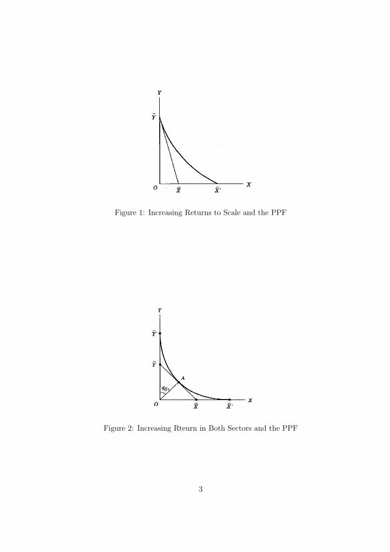
Figure 1: Increasing Returns to Scale and the PPF

Figure 2: Increasing Rteurn in Both Sectors and the PPF

3

Figure 3: Fixed Costs and the PPF

could be due to a large upfront investment or costs of entering an industry. A way to

represent fixed cost is to express it in terms of units of labor. So X requires a fixed amount

of labor, say F , as an upfront fixed cost. Once the fixed costs are paid, production of one

unit of X requires one unit of labor. The production Y also requires one unit of labor for

one unit of output, but there are no fixed costs in production of Y . The effect of fixed costs

is depicted in figure 3. When all the labor is allocated to sector Y , the maximum output

produced is Y . But, a reduction in output of Y will not result in production of X until the

fixed cost, represented by distance Y Fx, is paid. Having paid this cost, further reductions

in output of Y result in a constant (per unit of Y ) increase in output of X. Thus, the

production possibility frontier is given by Y FxX. In case there are fixed costs in both the

sectors, the production possibility frontier is given by Y FxFyX as depicted in figure 4.

In both cases, (i) production function is increasing returns and there are no fixed

costs and (ii) production function is constant returns to scale and there are fixed costs, the

problem is that the set of feasible points is not convex any more, i.e. points on a line joining

two feasible points may not be feasible.

Furthermore, with increasing returns, in equilibrium the price line is generally not

tangent to the production possibility frontier. The reason for this is that the marginal

products of factors rise when the production function is characterized by increasing returns.

With increasing returns, marginal product is greater than average product - the amount

4

Figure 4: Fixed Costs in Both Sectors and the PPF

produced by the last worker hired is greater than the average over all workers. Therefore, if

the firm paid all labor the value of marginal product of the last worker, it would lose money.

1 Economies of Scale

In some cases scale economies are external to individual firms, and occur at the level

of industry or groups of industries. An example is the agriculture industry. An individual

farm does not experience large economies of scale, but as the agricultural sector has grown

it has become profitable to produce specialized machinery and fertilizer, build railroads

and handling facilities and conduct research into better seed varieties. This has allowed to

production to expand and costs to fall for the sector as a whole, even though each individual

farm faces constant returns and acts as a price taker. In case of external economies of scale,

the problems discussed above with respect to incorporating scale economies in the general

equilibrium framework we have developed do no exist. Individual firms remain small with

respect to the market, so that we can still use the tools of competitive equilibrium.

On the other hand, internal economies of scale are economies of scale that are internal

to the individual firm and result from a large scale of production. Typical examples are ex-

tractive industries such as mining and petroleum, banking, finance and insurance. However,

internal economies of scale are usually inconsistent with perfect competition. To see this,

5

Figure 5: Internal Economies of Scale in Partial Equilibrium

suppose the total cost of a firm is given by: TCx = F +MCx.X, where F is a the fixed cost,

MCx is the marginal cost of production and X is the output level of the good. The idea

is that the firm must pay a fixed cost towards setting up the plant and equipment to start

production, but thereafter it can produce with constant returns to scale, or at a constant

marginal cost. Given this cost function, the average cost of the firm is ACx = F/X + MCx.

With the marginal cost constant, the average cost falls steadily as the fixed cost is spread

over a larger and larger output. Note that as the output increases the average cost approach

the marginal cost, but will be never equal to it. This situation is depicted in figure 5, along

with the marginal revenue (MR) and demand (D) curve for the firm.

If the price equals marginal cost, which in the figure is given by p = pc, the firm will

make a loss because it is always the case that the average costs exceeds the marginal cost -

ACx > MCx = p. At the price pc the output produced is Xc and the average cost is ACc.

Therefore, the loss of the firm is given by (pc − ACc).Xc. On the other hand if the price

exceeds the marginal cost and firms behave competitively, i.e. each firm believes that it can

sell all it wants at the given price. Since the average cost of each firm is falling, each firm

will try to sell an infinite - at some point the average cost will fall below the price and then

keep falling. Thus, no competitive equilibrium will exist in this case.

6

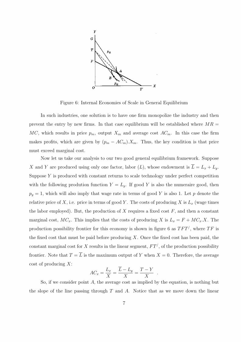
Figure 6: Internal Economies of Scale in General Equilibrium

In such industries, one solution is to have one firm monopolize the industry and then

prevent the entry by new firms. In that case equilibrium will be established where MR =

MC, which results in price pm, output Xm and average cost ACm. In this case the firm

makes profits, which are given by (pm − ACm).Xm. Thus, the key condition is that price

must exceed marginal cost.

Now let us take our analysis to our two good general equilibrium framework. Suppose

X and Y are produced using only one factor, labor (L), whose endowment is L = Lx + Ly.

Suppose Y is produced with constant returns to scale technology under perfect competition

with the following prodution function Y = Ly. If good Y is also the numeraire good, then

py = 1, which will also imply that wage rate in terms of good Y is also 1. Let p denote the

relative price of X, i.e. price in terms of good Y . The costs of producing X is Lx (wage times

the labor employed). But, the production of X requires a fixed cost F , and then a constant

marginal cost, MCx. This implies that the costs of producing X is Lx = F + MCx.X. The

production possibility frontier for this economy is shown in figure 6 as TFT /, where TF is

the fixed cost that must be paid before producing X. Once the fixed cost has been paid, the

constant marginal cost for X results in the linear segment, FT /, of the production possibility

frontier. Note that T = L is the maximum output of Y when X = 0. Therefore, the average

cost of producing X:

ACx =Lx

X=

L − Ly

X=

T − Y

X.

So, if we consider point A, the average cost as implied by the equation, is nothing but

the slope of the line passing through T and A. Notice that as we move down the linear

7

segment of the production possibility frontier, FT /, the slope of such a line decreases. This

implies that the average cost of X decreases as the production of X increases, indicating

increasing returns. For a positive X to be produced at non-negative profits the price line

must cut the production possibility frontier. This means that the slope of the price line is

greater than the slope of the production possibility frontier - p > MCx. The slope of the

segment FT / is the nothing but the constant MCx.

For strictly positive profits for the monopolist, the price line through the equilibrium

point must be steeper than the average cost line. Point A is such an equilibrium because the

the price line pa is steeper than the average cost line TA. The distance OT is the maximum

output of Y , and therefore it is also the total labor income L. The distance GT is the profit

of the monopolist. The budget line of the wage earnersis given by the line with slope pa

through T = L. Point B is the consumption equilibrium for labor income. Therefore, the

difference between bundles B and A is the consumption out of profit income. Since wage

earner’s income is fixed in terms of Y at T = L, a decline in the price of good X, p, will

cause the budget line to swivel (rotate) around the fixed point T . Notice that is the profits

are zero, which happens if the price line overlaps the average cost line TA, the consumption

out of profits is zero and point B will coincide with A.

From national income accounts perspective, in this setting with only one factor, wage

income plus profits will give the GNP (gross national product) of the country. When we

introduce trade in this model, the GNP will change because of change in workers’ utilities

and/or changes in monopoly profits.

2 Gains from Trade Under Monopolistic Competition

In the Ricardian and HO models we assumed that markets were perfectly competitive

- large number of firms produced and sold a homogeneous (identical) product. However,

these models fail to explain trade between rich countries. This is because rich countries

do not differ much from each other in technology as well as in endowments of resources.

Furthermore, rich countries export and import similar products. This is also called two-way

trade. To explain trade between rich countries we will adopt the framework of monopolistic

competition. The main features of this model are:

8

1. There are many firms in an industry, and each firm produces a good that is similar

but differentiated from goods that other firms in the industry produce. For example,

in a store we can find many different types of detergents. Because each firm’s product

can be differentiated from the products of other firms a firm can raise the price of its

product without losing all of its customers. Thus, each firm faces a downward sloping

demand curve for its product and has some market power.

2. Firms produce using a technology with increasing returns to scale. Due to increasing

returns to scale production technology, the average cost of a firm will fall as the firm

produces more. As a result the marginal cost will always be lower than the average cost

(example - if the class average grade falls when a new student joins the class it must be

that the new student’s grade is below the existing class average). Because firms have

some market power they will be able to charge a price higher than marginal costs, and

when the price charged is higher than average costs they will make monopoly profits.

3. Firms can enter or exit the industry freely. Free entry and exit of firms will ensure

that the profits of each firm are zero in the long-run. This is because as long as firms

in an industry are making profits it will lead to entry of new firms which will results

in lower profits for all firms. Hence in the long-run there will be no entry when profits

of all firms in an industry are zero.

Potential gains from trade in the presence of increasing returns can come from different

sources:

2.1 Pro-Competitive Gains

Scale economies imply that the market can support only a limited number of firms,

which means that the market is imperfectly competitive. Trade, by expanding the size of

the market, helps to support a larger number of firms and thereby increases the level of

competition. This is the pro-competitive gains from trade. The effect shows up in the form

of a decrease in the markup of a firm for a given level of output and/or an expansion of the

output of the firm with resulting capture of price over marginal cost. We are going to adopt

9

the latter definition, which is often called the product-expansion effect. Remember, from our

analysis from the previous chapter, an increase in the output of industry which is imperfectly

competitive is welfare improving since it reduces the price and therefore the economy captures

the excess of price over marginal cost for the additional output produced. To see this, note

that the total cost of producing X amount of good X can be written as TCx = X.ACx, which

implies that the change in total cost is given by ∆TCx = ACx.∆X + X∆ACx. Dividing

both sides of this expression by ∆X gives us the marginal cost.

MCx =∆TCx

∆X= ACx + X

∆ACx

∆X.

Then the gain from the product-expansion effect is given by:

(p − MCx).∆X = (p − ACx).∆X − X∆ACx

∆X.∆X .

Thus the pro-competitive (product-expansion) effect can be decomposed into two compo-

nents. The first term on the right-hand side is the profit effect and the second term is the

decreasing average cost effect. The profit effect captures the fact that if the price exceeds the

average cost, then the additional output generates a profit which is a part of the national

income. The second term captures the effect that with increasing returns the change in

average cost due to an increase in output is negative, which combined with negative sign in

front of this term means that it has welfare improving effect. This is because the average

cost of producing the initial output X is lower now.

Note that the profit effect, ultimately, due to trade may shrink to zero, i.e. price

will equal average cost. However, during this process of shrinking profits the economy will

capture the excess of price over average cost on each additional unit till profit becomes zero.

Furthermore, in the case of external economies to scale where price is equal to average cost

for each firm, the profit effect is zero. Unlike the profit effect, which arises from imperfect

competition, the decreasing average cost effect can occur only with increasing returns. In case

of imperfect competition with constant returns to scale, average and marginal cost would be

the same, and we would have only the profit effect. Figure 7 shows the decomposition of the

pro-competitive effect. The initial equilibrium is at point A with price ratio p. Suppose, the

with trade p (hypothetically) remains unchanged but the output of X expands to point Q.

10

Figure 7: Decomposition of the Pro-Competitive Effect

The movement from A to Q can be decomposed into movement from A to B and movement

from B to Q. The movement from A to B is the expansion in output holding the average

cost constant at the initial level ACx0, which is why point B lies on the initial average cost

line. Thus, this captures the profit effect. The movement from B to Q is captures the decline

in the average cost from ACx0 to ACxf , captured by the decline in the slope of the average

cost line, at the same level of output Xf . Hence, this captures the declining average cost

effect.

Notice that if the price ratio p equaled the initial average cost ACx0, then there would

be no profit effect and hence the movement from A to Q would be entirely the decreasing

average cost effect. On the other hand, if there fixed costs then the slope of the average

cost line would coincide with the slope of the production possibility frontier and hence there

would be no decreasing average cost effect, implying that the movement from A to Q would

entirely due to the profit effect.

We could generalize this analysis to a case of two identical countries, with each country

having increasing returns in sector X and competitive industry in sector Y . The autarky

equilibrium point is A in figure 8. With trade, we assume that the two monopoly producers

in sector X compete in quantity - cournot competition. As a result, the two producers

perceive demand to be more elastic thereby reducing the markup and hence the price, which

11

Figure 8: Cournot Competition and Pro-Competitive Gains

in turn results in higher output. The final equilibrium could be achieved at point Q at price

ratio p∗, with no net trade between the identical countries, but still gains from trade - utility

level of each country increases from Ua to Uf . This pro-competitive gains is due to both the

profit effect and the decreasing average cost effect.

2.2 Firm Exit Effect

Scale economies imply that it is more efficient for one firm to cater to the entire market.

However, with one or very few firms the market power of the individual firm is higher, which

implies a lower output level. This trade-off results in a third source of gains from trade -

firm exit effect. The idea is that trade will increase the total number of firms in competition

while reducing the number of firms in each individual country. The key here is that initially

in autarky there is free entry of firms, so that the profits are forced down to zero. Trade

causes each firm to perceive the demand to be more elastic resulting in an increase in output

by each firm, and some firms will then exit as profits are initially negative. Thus, in the

trading equilibrium, each country will have fewer firms, with each firm producing a higher

output at lower average cost.

The firm exit effect is illustrated in figure 9. Autarky equilibrium is at point A for each

of the two countries. Due to free entry the prices are forced down to the level of the average

12

Figure 9: Firm Exit Effect

cost, and the vertical distance TF / is now interpreted as the combined fixed costs of the

existing firms. When these economies open up to trade, each firm perceives is demand curve

as more elastic and therefore increases its output. But, this leads to negative profits and the

exit of some firms. The new equilibrium is established at a lower price, with fewer firms in

each country but more firms in total. The exit of loss making firms frees up resources that

were being used to pay the fixed costs and shifts the production function of each country

out to TFT //. The new consumption point for both countries is C. It is possible that at

the new equilibrium there is no net trade because the two countries are identical and attain

the same consumption equilibrium.

The movement from A to C is a combination of the pro-competitive effect and the firm

exit effect. The movement from A to B does not involve any exit of firms because the total

resources going towards the fixed cost are the same (TF /). Thus this movement involves a

pure expansion of output, holding the number of firms constant. This, therefore, captures

the pro-competitive effect. The movement from B to C captures the firm exit effect. Notice

that the average cost at C and at B is the same (given by the slope of the line TCB).

Therefore, the the output per firm must be the same at the two points. As a result, the

movement from B to C is a reduction in the number of firms, holding the outputs surviving

firms constant, and therefore captures the firm-exit effect.

13

2.3 Increased Product Diversity

In a perfectly competitive industry there is no product diversity because the all firms

produce identical products, i.e. there is no product differentiation. However, in a monopo-

listically competitive industry, with large number of firms, each firm produces a somewhat

unique product which is why each firm faces downward sloping demand curve. However, the

existence of a demand for each firm, and therefore each product, implies that the consumers

like variety/diversity. Such preferences are often called the love of variety preferences.

To see the role of this channel, lets assume that both X and Y are produced with

increasing returns technologies that are identical. Furthermore, the two goods are symmetric

but imperfect substitutes in consumption, i.e. consumers are indifferent between one unit

of X and one unit of Y , but they would like to consume some of both rather than more of

just one. The autarky equilibrium for both countries is attained at point A, in figure 10.

However, this is not the best choice even in autarky. The large fixed costs imply that it is

not beneficial for the country to produce both goods. It would be better of by specializing

in either Y at point T or in X at T / as it would put the country on higher indifference

curve, which would pass through T and T /. In such as case benefits from product variety

are outweighed by the fixed costs of producing another good. With trade, each country

can specialize in one of the goods and trade half of its output for half of the output of the

other country’s good. This will allow countries to consume at point C. This move from

A to C does not involve any change in the average cost of producing a good and does not

involve any pro-competitive gains. Thus, trade allows both varieties to be consumed in each

country (as against only one in autarky) with the opportunity for countries to specialize in

the production of only one of the varieties.

Another way to think about love of variety is to think in terms of an ideal variety of a

consumer depending on the consumer’s taste and income level. Because of scale economies,

no country can afford to produce the ideal variety of each consumer. For example, Ger-

many produces Volkswagens and Mercedes-Benzes, France produces Renaults and Peugeots

whereas Japan produces Honda and Toyota. Trade in automobiles occurs among these

countries because there are consumers in each country that like varieties of automobiles not

14

Figure 10: Love of Variety and Gains from Trade

produced in their own country. This situation is depicted in figure 11. Suppose automobiles

have only two characteristics on the basis of which they can be differentiated - size and

fuel efficiency. However, there is a trade-off between these two - bigger cars have lower fuel

efficiency. Figure 11 shows three possible combinations of size and fuel efficiency, denoted

X, Y , and Z, corresponding to three different types of cars. Suppose all three models could

be produced at the same average cost for the same level of output. There are two types of

consumers - students and faculty. Students like fuel efficient cars, whereas faculty prefers

size over fuel efficiency. The indifference curves for the two groups are denoted by Us and

Uf , respectively.

However, the presence of scale economies will make it more efficient to produce just one

model, instead of producing two models that will appeal to each kind of consumer. Thus,

it possible that in autarky a country just produces Y , which sells for a modest cost, but

faculty are cramped and students are poor from paying from gas. The utility levels of the

two groups are U/f and U

/s , respectively. However, trade with a second identical country will

allow one country to produce X and other to produce Z, each exporting half of its output

for half of the other country’s output. Each country will produce the same number of cars

as in autarky, and consequently cars would have the same average cost. Assuming X and Z

sell for the same price as Y did in autarky, consumers will pay the same for cars but attain

15

Figure 11: Ideal Variety

a higher utility, Uf and Us, because of the availability of their ideal variety. Thus, the gains

from trade are, again, in terms of greater variety rather than in terms of a decline in price.

3 Increasing Returns and Factor Returns

Up until now we had focused on production with one factor, labor. However, in the

Heckscher-Ohlin world of two factors, or in fact in world with more than two factors, trade

in the presence of increasing returns may benefit all factors in real terms. This could either

due to decline prices of goods or an increase in welfare due to availability of a larger variety

of goods.

4 Empirical Evidence on Gains from Trade Under Scale

Economies

Most economist regard scale economies as an important determinant of international

trade. The idea that free trade will expand the range of products available to consumers

16

is not new. David Ricardo, in chapter 7 of his book “On the Principles of Political

Economy and Taxation”, wrote -

Foreign Trade, then,...[is] highly beneficial to a country, as it increases the amount and

variety of the objects on which revenue may be expended.

However well grounded theoretical developmet of this idea happened in the 1980s by

Elhanan Helpman, Paul Krugman, and the late Kelvin Lancaster. The research was

not just theoretical; it was used to understand free-trade agreements and their effects on

domestic output, productivity, factor returns, and gains from trade. We will use NAFTA to

illustrate gains and costs predicted by the monopolistic competition model.

4.1 Case Study: Effect of NAFTA on Canada

Studies in Canada as early as the 1960s predicted substantial gains from free trade with

the U.S. The main ideas was that Canadian firms would expand their scale of operations to

service the larger market (U.S.) and lower their costs. Studies by Richard Harris in the mid-

80s, based on the monopolistic framework, influenced Canadian policy makers to proceed

with the free trade agreement with the U.S. in 1989.

Data from 1988-1996 was used by Daniel Trefler (of Univ. of Toronto) to estimate

effects of NAFTA on Canada in his paper titled “The Long and Short of the Canada-

U.S. Free Trade Agreement” (published in the American Economic Review in 2004).

Here are some findings:

4.1.1 Productivity and Real Wages

1. In the long run, large positive effects on productivity were found.

• 15% over eight years in industries most affected by tariff cuts - compound growth

of 1.9% per year.

• 6% for manufacturing overall - compound growth of 0.7% per year.

• The difference between the two numbers, above, of 1.2% per year is an estimate

of how free trade with the U.S. affected the Canadian industries over and above

the impact on other industries.

2. The productivity growth led to a rise of 3% in real earnings over this period.

17

4.1.2 Adjustment Costs

1. Short-run adjustment costs of 100,000 jobs, or 5% of manufacturing employment.

2. Some industries that had very large tariff cuts saw employment fall by as much as 12%.

3. Over time, however, these job losses were more than made up for by creation of new

jobs elsewhere in manufacturing. There were no long run job losses due to NAFTA.

Notice that the gains from trade due to the increase in the number of varieties available

after trade were not estimated by Trefler.

4.2 Case Study: Effect of NAFTA on Mexico

In the mid-1980s, Mexican President Miguel de la Madrid initiated economic reforms

that included land reform and greater openness to foreign investment. Tariffs with United

States were as high as 100% on some goods, and there were many restrictions on the opera-

tions of foreign firms. Joining NAFTA was a way to ensure the permanence of the reforms

already underway. Under NAFTA, Mexican tariffs on U.S. goods declined from an average

of 14% in 1990 to 1% in 2001. In addition, U.S. tariffs on Mexican imports fell as well. We

look at growth in labor productivity and real wages, and adjustment costs in Mexico based

on the analysis carried out by Gary C. Haufbauer and Jeffrey J. Schott in their 2005

paper titled “NAFTA Revisited: Achievements and Challenges.”

4.2.1 Productivity and Real Wages

To evaluate the effect of NAFTA on productivity growth in Mexico we compare labor

productivity growth of maquiladora plants with that of non-maquiladora plants. Since the

maquiladora plants produce almost exlusively for export to the United States, these should

be most affected by NAFTA.

1. For the maquiladora plants, productivity grew from 1994 to 2003 at a compound growth

rate of 4.1% per year.

18

2. For non-maquiladora plants, productivity grew at a compound growth rate of 2.5% per

year.

3. The difference, 1.6% per year, is an estimate of the impact of NAFTA on the produc-

tivity of maquiladora plants over and above the increase in productivity that occurred

in the rest of Mexico.

To see the effect of NAFTA on real wages we compare real wages in the maquiladora

plants with those in the non-maquiladora plants.

1. From 1994 to 1997, there was a fall of over 20% in real wages in both sectors, even

with increase in productivity. Why did this happen?

• Shortly after joining NAFTA, Mexico suffered a financial crisis that led to a large

devaluation of the peso.

• The maquiladora sector was mostly affected by devaluation of peso and did not

experience much productivity gain as the devaluation made it more expensive for

Mexico to import goods.

• Workers in both areas had to pay higher prices for imported goods - higher Mex-

ican consumer prices.

• Decline in real wages was similar for both sectors.

2. The decline was, however, short lived. Real wages in both sectors began to rise again

in 1998. By 2003, real wages were back to their 1994 value.

3. Sadly, the productivity gains were not shared with workers. If we look at real monthly

income, the picture is a little better. This includes other sources of income beside

wages, especially for higher-income persons.

• For non-maquiladora sector, data on real wages and real monthly income move

together closely.

• In the maquiladora sector, real incomes were higher in 2003 than in 1994. Some

gains for workers in plants most affected by NAFTA.

19

4. Higher-income workers fared better than unskilled workers in Mexico. Those in maquiladora

sector are principal gainers due to NAFTA in the long run.

4.2.2 Adjustment Costs

1. When Mexico joined NAFTA, it was expected that the agricultural sector would fare

the worst due to competition from the U.S.. And, therefore tariff reductions in agri-

culture were phased over 15 years. The evidence to date shows the corn farmers did

not suffer as much as was feared. Surprisingly, total production of corn in Mexico rose

following NAFTA. Why?

• The poorest farmers consume the corn they grow, not sell it.

• Mexican government was able to use subsidies to offset the reduction in income

for other corn farmers.

2. For maquiladora plants, employment grew rapidly following NAFTA to a peak of 1.29

million in 2000. After that, this sector entered a downturn. Employment in the

maquiladora sector fell after 2000 to 1.1 million in 2003.

• The U.S. entered a recession decreasing demand for Mexican exports.

• China was competing for U.S. sales by exporting goods similar to those sold by

Mexico.

• The Mexican peso became over-valued, making it difficult to export abroad.

3. The maquiladora sector faces increasing international competition (not all due to

NAFTA). This can be expected to raise the volatility of its output and employment.

The volatility can be counted as a cost of international trade for workers who are

displaced.

4.3 Case Study: Effect of NAFTA on United States

Studies on the effects of NAFTA on the U.S. have not estimated its effects on the

productivity of U.S. firms. It would be hard to identify the impact since Mexico and Canada

20

are only two of many trading partners. Instead, researchers have estimated the second source

of gains from trade: the expansion of import varieties available to consumers. For U.S. we

will compare the long-run gains to consumers due to expanded product varieties with the

short-run adjustment costs from exiting firms and unemployment.

4.3.1 Expansion of Variety to the U.S.

To understand how NAFTA affected the range of products available to U.S. customers, we

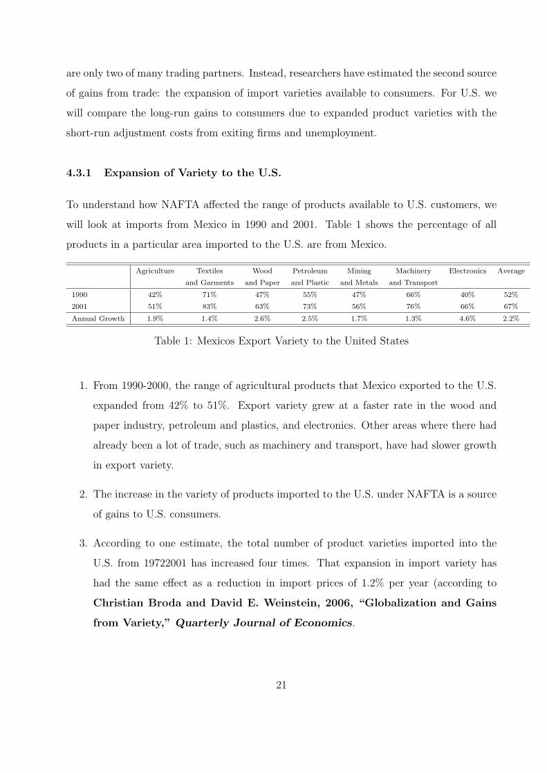
will look at imports from Mexico in 1990 and 2001. Table 1 shows the percentage of all

products in a particular area imported to the U.S. are from Mexico.

Agriculture Textiles Wood Petroleum Mining Machinery Electronics Average

and Garments and Paper and Plastic and Metals and Transport

1990 42% 71% 47% 55% 47% 66% 40% 52%

2001 51% 83% 63% 73% 56% 76% 66% 67%

Annual Growth 1.9% 1.4% 2.6% 2.5% 1.7% 1.3% 4.6% 2.2%

Table 1: Mexicos Export Variety to the United States

1. From 1990-2000, the range of agricultural products that Mexico exported to the U.S.

expanded from 42% to 51%. Export variety grew at a faster rate in the wood and

paper industry, petroleum and plastics, and electronics. Other areas where there had

already been a lot of trade, such as machinery and transport, have had slower growth

in export variety.

2. The increase in the variety of products imported to the U.S. under NAFTA is a source

of gains to U.S. consumers.

3. According to one estimate, the total number of product varieties imported into the

U.S. from 19722001 has increased four times. That expansion in import variety has

had the same effect as a reduction in import prices of 1.2% per year (according to

Christian Broda and David E. Weinstein, 2006, “Globalization and Gains

from Variety,” Quarterly Journal of Economics.

21

4. If we use the 1.2% equivalent reduction in import prices for Mexico that has been found

for all countries, we can estimate some dollar gains. Using an average $90 billion in U.S.

imports per year and the 1.2% reduction in prices to U.S. consumers, $90(1.2%) = $1.1

billion per year in savings to consumers.

5. These consumer savings are permanent and increase over time as export varieties grow.

Over the first nine years of NAFTA, the total benefit to consumers was $49.5 billion,

or an average of $5.5 billion per year.

4.3.2 Adjustment Costs in U.S.

These come as firms exit the market due to import competition and the workers employed

there are temporarily unemployed. One way to measure this loss is to look at claims under

the U.S. Trade Adjustment Assistance (TAA) provisions. This program offers assistance to

workers in manufacturing who lose their jobs due to import competition.

1. From 1994-2002, about 525,000 workers, or about 58,000 per year, lost their jobs and

were certified as adversely affected by trade under the NAFTA-TAA program.

2. We can compare this number to overall job displacement in the U.S. over the same

time period. The annual number of workers displaced in manufacturing was 4 million

or 444,000 workers per year.

3. The NAFTA layoffs of 58,000 workers were about 13% of total displacementthis is a

substantial amount.

Another way to measure effects are to compare the loss in wages from the displaced

workers to the consumer gains.

1. It is estimated that about 2/3 of workers laid off in manufacturing are re-employed

within three years. Suppose the average length of unemployment for laid off workers

is 3 years.

22

2. Average yearly earnings for manufacturing workers was $31, 000 in 2000 so each dis-

placed worker lost $93, 000 in wages.

3. Total losses were $5.4 billion for the U.S. economy.

4. These private costs of $5.4 billion are nearly equal to the average welfare gains of $5.5

billion.

However, gains continue to grow over time as new imported products become available to

U.S. consumers and job loss is only temporary. Thefefore, adjustment costs due to job losses

fall.

4.4 Case Study: Summarizing the Effects of NAFTA

1. We have been able to measure in part the long-run gains and short-run costs from

NAFTA for Canada, Mexico, and the U.S.

2. The monopolistic competition model indicates two sources of gains from trade.

• The rise in productivity due to expanded output by surviving firms, which leads

to lower prices.

• More varieties of products for consumers.

3. For Mexico and Canada, long-run gains were measured by the improvement in pro-

ductivity for exporters as compared to other manufacturing firms. For the U.S., we

measured the long-run gains using the expansion of varieties from Mexico, and the

equivalent drop in price faced by U.S. consumers.

4. It is clear that for Canada and the U.S., the long-run gains considerably exceed the

short-run costs.

5. In Mexico the gains have not been reflected in the growth of real wages for production

workers.

• The real earnings for higher-income workers in the maquiladora sector have risen

and have been the principal beneficiaries of NAFTA so far.

23