Paper for the 43rd European Congress European Regional Science Association (ERSA)

August 27-30, 2003. Jyväskylä, Finland

Increasing Returns and Spatial Unemployment Disparities Jens Suedekum*) University of Goettingen, Germany

ABSTRACT Standard models of the new trade and location theories usually assume full employment and are thus ill-equipped to study spa-tial unemployment differences, which in reality are more pro-nounced that income disparities. Regional labour market theo-ries like the ´wage curve´-approach on the other hand can not endogenously explain the origin of regional economic dispari-ties. We analyse regional agglomeration and regional unem-ployment in an unified approach by combining a wage curve with an increasing returns technology. We find that regional unemployment rates closely resemble the core-periphery struc-ture of regional GDP per capita. This matches the stylised facts from EU-15.

JEL Classifications: F4, J6, R1. Keywords: Regional Unemployment, Economic Geography,

Increasing Returns, Wage Curve, Migration, Labor Mobility. *) Correspondance address: Jens Suedekum, Department of Economics, University of Goettingen. Platz der Goettinger Sieben 3, 37073 Goettingen, Germany. Phone: +49/551/39-7633. jsuedek@gwdg.de The author is grateful to Federico Cingano, Harry Garretsen, Andreas Haufler, Michael Pflueger and Peter Ruehmann for several very useful comments on an earlier version of this paper. Of course I am fully responsible for all remaining errors.

2

1) Introduction

Economic activity differs markedly across European regions. People from the richest

European regions (London, Brussels, Luxemburg, Hamburg) have an average real pur-

chasing power about five times higher than people from the poorest areas (Ipeiros,

Acores). Spatial divides are even larger with respect to unemployment rates. In the

European Union today, regions with practically full employment and regions with ex-

cessive mass unemployment coexist. In many cases they coexist even within the same

country. Germany, Italy and Spain are the most prominent examples, where some re-

gions have unemployment rates below 5 per cent, whereas others are stuck with figures

well above 20 per cent. Such spatial unemployment disparities within and across coun-

tries exist for decades. In recent years, there was even a tendency for them to increase.

Moreover, regional unemployment rates in the EU follow a quite distinct spatial pattern

of trans-national clusters that closely resembles the core-periphery-structure of regional

GDP per capita (see section 2). Regional unemployment rates are low in the rich core

regions of the European Union, where population, production and income are agglom-

erated. On the contrary, high unemployment rates are found in the small and economi-

cally peripheral regions with low levels of output and income per capita. National bor-

ders do not play a very dominant role in this division scheme of areas with low, inter-

mediate and high unemployment rates.

The main aim of this paper is to explain this spatial coincidence of low (high) unem-

ployment and high (low) GDP per capita-levels in the NUTS2-regions of EU-15. Put

differently, we aim to explain the spatial structure of regional unemployment rates

within an integrated economic area like the EU in relation to the corresponding regional

economic agglomeration. This is a largely unexplored issue in the literature.

Unemployment has always been a prominent topic for macroeconomists, who predomi-

nantly think in national dimensions. Regional issues traditionally play a minor role in

this debate. However, regional labour market analysis has gained some prominence dur-

ing the last years. One useful regional approach comes from David Blanchflower and

Andrew Oswald (1990, 1996), who have compiled a great deal of empirical evidence

about regional labour markets and claim to have distilled an “empirical law” of econom-

ics from the data, known as the wage curve. The wage curve theory is useful for our

purposes, since it draws an inherent link between key labour market variables on a re-

gional level, namely the unemployment rate and the real wage level. But the existing

wage curve models alone are insufficient to understand the regional dimension of eco-

3

nomic activity in the EU. This is so, because one can not endogenously explain why

there are so pronounced core-periphery divides in production and income across space

with the Blanchflower/Oswald-model, effectively because it leaves no room for en-

dogenous agglomeration forces.

The vastly growing field of economic agglomeration theories are the second string in

the literature that our theoretical analysis relates to, namely the theories now known as

the “new trade theory (NTT)” and “new economic geography (NEG)” (Krugman, 1980,

1991). Especially the latter can be seen as a modern theory of regional agglomeration

that explicitly shows how core-periphery divides of economic activity can endoge-

nously emerge and persist within an integrated area due to the presence of localised in-

creasing returns to scale. Nevertheless, this vastly growing literature usually has nothing

to say about unemployment. The models of NTT and NEG mostly assume that labour

markets always automatically clear.11 The phenomenon of regional unemployment dis-

parities can thus not be analysed explicitly.

We will therefore propose a theoretical framework in this paper that attempts to close

this gap in the literature. Our aim is to marry a wage curve, which is thought of as a

labour market equilibrium curve, with a product market that exhibits the essential fea-

tures of the new regional agglomeration theories. The innovation from a theoretical

point of view is twofold: Firstly, our model can be seen as an improvement of the gen-

eral equilibrium approach from Blanchflower/Oswald, since the regional disparities can

develop endogenously. And secondly, it is an attempt to introduce the element of unem-

ployment to the new regional agglomeration theories. Our main finding is that large

core regions with high per capita income levels have low unemployment rates and vice

versa. Hence, our theoretical framework implies results that are consistent with the styl-

ised facts about regional unemployment disparities and regional agglomeration in the

EU as a whole.

The rest of this paper is organized as follows. After a brief overview about regional dis-

parities in the EU in section 2, we introduce the essential ideas of the wage curve model

of Blanchflower/Oswald in section 3. In section 4 we point to some problems of this

model and argue that it alone is ill-equipped to understand the regional labour market

disparities in the EU. Our own model structure with an increasing returns technology,

1 The notable exceptions in this respect are Peeters/Garretsen (2000) and Matusz (1996), whose focus, however, is somehow different, namely on the overall impact of globalisation on unemployment.

4

which is designed to cope with these problems, is introduced in section 5. Section 6 then

provides a discussion of this approach as well as some concluding remarks.

2) Regional economic disparities in the European Union

In almost all EU member countries there exist non-negligible, in some cases even ex-

treme intra-national unemployment disparities on the usual level of regional gradation,

NUTS2. Figure 1 shows the region with the lowest and the highest unemployment rate

in 2000 for those 13 EU-countries that consist of more than one NUTS2-region.2

As can be seen, the intra-national differences in some countries are by far more pro-

nounced than the differences between countries. Most notably this is so in Italy, Spain

and Germany. But also in some smaller countries, e.g. Finland, Belgium and Greece,

differences are significant and range around 9-10 percentage points.

Figure 1: EU-15 – Regional Unemployment Disparities 2000

Country (national unemp. rate)

Min-region Max-region Difference

Italy (10,8) Trentino/Alto Adige (3,1)

Calabria (27,7) 24,6

Spain (14,4) Navarra (4,9) Ceuta y Mellila (25,5) 20,6 Germany (8,1) [West Germany]

Oberbayern (3,5)

Halle (19,2) [Bremen (10,5)]

15,7 [7,0]

Finland (11,0) Aland (1,7) Ita Suomi (15,5) 13,8 France (9,6) Alsac (5,3) Languedoc-Rousillon (16,1)

[Réunion (33,1)] 10,8 [27,8]

Belgium (6,7) Vlaams Brabant (2,9) Hainaut (13,1) 10,2 Greece (11,1) Ionia Nisia (5,1) Dytiki Makedonia (14,7) 9,6 UK (5,6) Berkshire (1,9) Merseyside (11,2) 9,3 Sweden (6,2) Stockholm (3,6) Norra Mellansverige (8,8) 5,2 Portugal (4,1) Centro (1,8) Alentejo (5,7) 3,9 Austria (3,9) Oberösterreich (2,6) Wien (5,8) 3,2 Netherlands (2,8) Utrecht (2,1) Groningen (4,6) 2,5 Ireland (4,4) Southern/Eastern (3,9) Midland/Western (5,8) 1,9

Source: Eurostat. European Commission.

But let us also look at the European Union as a whole from a bird’s perspective. The

maps 1 and 2 in the appendix show regional unemployment rates and regional GDP per

capita for the EU-27. When focussing on the current EU-members (EU-15), the maps

2 Denmark and Luxemburg are not further divided below the level of NUTS0.

5

reveal a quite distinct spatial pattern that could be described as a figure of concentric

circles.

There is an area, geographically located in the middle of the continent, where unem-

ployment rates are on a very low level. This core area contains Northern Italy, Southern

Germany and Austria, the Netherlands and the southern part of Great Britain. Map 2

makes clear that the highest levels of regional GDP per capita are found precisely in this

area, which is often called the „European banana“, where economic activity is highly

agglomerated.3

Exactly the opposite characteristics can be found in the geographically remote areas at

the outside borders of EU-15. The regions in Southern and Easters Spain, Southern It-

aly, Greece and Eastern Germany have high or very high unemployment rates. They all

belong to the group of regions with a GDP per capita level below 75 per cent of the EU-

15-average and are thus eligible for “objective 1”-funding from the EU structural funds.

Yet, not all “objective 1”-regions have mass unemployment. The notable exception is

Portugal. All Portuguese are relatively poor, but unemployment rates are modest. One

might thus put it this way: Belonging to the group of “objective 1”-regions is a neces-

sary, but not a sufficient condition for having extraordinarily high unemployment rates.

All in all, however, “objective 1” regions on average have unemployment rates well

above the EU-average (15,8% vs. 9,7% in 1999).

In between these two trans-national clusters, there is a group of regions with intermedi-

ate income levels and unemployment rates. This group contains most parts of France,

Eastern Spain, the middle part of Italy, North-Western Germany, Scandinavia and the

Northern part of UK. In a stylised manner, the geographic structure of income and un-

employment can thus be characterised as in figure 2.

Figure 2 casts some doubts whether it is really useful to predominantly think about un-

employment along national borders. In fact, regional unemployment rates in the EU-15

seem to follow a trans-national core-periphery structure that closely resembles the spa-

tial configuration of GDP per capita.4 Put differently, the membership of a specific re-

3 The regions in this central area reveal also some other favourable economic characteristics, like a high participation rate, a high fraction of skilled labour and a high innovative activity (Suedekum, 2003a; EU-Commission, 2001). 4 See also CER (1998): “the high unemployment regions in Europe have a low per capita income (30% below the EU average) and a similar production structure, in which manufacturing represents a lower than

6

gion to one of the three income clusters („European banana“, “objective-1“, “intermedi-

ates”) seems to be a much more reliable indicator for the regional unemployment rate

than the assignment to a nation.

Figure 2: The regional dimension of economic activity in the EU-15

Overman/Puga (2002) call this phenomenon the “neighbouring effect“, according to

which there is a much higher similarity of unemployment rates between regions from

different countries that are geographically close to each other than between the unem-

ployment rate of a particular region with the respective national average.5

This spatial pattern is probably the result of an intra-national divergence and polarisa-

tion process of regional unemployment rates that occurred over the last 15 years or so.

Overman/Puga (2002) and Puga (2002) show that regions that used to have compara-

average share of output and is characterized by technologically stagnant industries such as food, mining, leather and apparel. On the contrary, the low unemployment regions are characterized by a 10% higher than average per capita income and a production structure in which manufacturing is prominent and di-versified, with a prevalence of industries such as machinery, precision instruments and electronics”. 5 The authors also show that there is a truly spatial dimension in European unemployment, since the simi-larity between unemployment rates of remote areas with a comparable sectoral structure is significantly weaker than between regions that are in close proximity to each other (Overman/Puga, 2002).

„Objective 1“-regions: Southern and Eastern Spain, Southern Italy, Greece, Eastern Germany, [Portugal]. - low GDP per capita - high unemployment rates - other unfavourable characteristics

The „European banana“: Southern Germany, Northern Italy, Southern UK, most of Benelux. - high GDP per capita - low unemployment rates - other favourable characteristics

The „intermediates“: Most parts of France, Northwestern Germany, Northern UK, Western Spain, Middle Italy, Scandinavia - intermediate levels of GDP per capita and unemployment rates.

7

1986

Une

mpl

oym

ent R

ate

tively high unemployment rates in 1986 usually also have high unemployment rates in

1996. The same is true for regions with comparatively low unemployment rates, but not

for those regions that had unemployment rates around the European average in 1986.

The unemployment rates of these areas often moved to either of the two extremes, and

only a small fraction of regions remained in range with intermediate relative unem-

ployment rates. This can be seen by the transition probability matrix in figure 3 that is

taken from Puga (2002). The matrix is constructed in the following way: The unem-

ployment rates of the European NUTS2-regions relative to the EU-average are divided

into five groups. The numeric values in the matrix are the relative frequencies of group

membership in 1996, given the information about the group assignment in 1986. Hence,

along the main diagonal there is the fraction of regions that ended up in the same range

in 1986 and 1996.

The table shows that there is a high degree of inertia for the groups with high and low

unemployment rates, but far less in the intermediate ranges. Many of those regions with

relative unemployment rates from 0.6 to 1.3 of the European average in 1986 (mainly

regions from France, Italy and Spain) moved either of the two extreme groups.

Figure 3: Transition probability matrix of regional unemployment rates

< 0.6 0.6-0.75 0.75-1.0 1.0-1.3 >1.3

< 0.6 0.81 0.19 0.00 0.00 0.00

0.6–0.75 0.52 0.26 0.09 0.09 0.04

0.75-1.0 0.24 0.29 0.26 0.21 0.00

1.0-1.3 0.06 0.22 0.34 0.19 0.19

> 1.3 0.00 0.00 0.16 0.22 0.62

Source: Puga (2002)

The polarisation process has not been reversed since 1996, but rather got more extreme

(Suedekum, 2003a). Furthermore, one can show that the described process was mainly

driven by the labour demand side rather than by labour supply. By definition, a regional

unemployment rate changes either because of a rise or decline of labour force participa-

tion (labour supply), or of employment (labour demand). It seems to be the case that the

1996 Unemployment rate

8

successful central regions with low and declining unemployment rates on average also

experienced an increase of labour supply by receiving internal migrants from other

European regions (EU-Commission, 2001). The rise in labour supply, however, was

outperformed on average by a stronger increase in labour demand (Martin/Tyler, 2000).

In other words, the core regions (which mostly already had a significantly higher popu-

lation density) managed to integrate more people into their labour markets, including

the internal migrants, and thus saw unemployment rates fall. The already sparsely popu-

lated sending regions on the other hand, where competition on the labour supply side

was even relaxed through emigration, nevertheless faced high and rising unemploy-

ment.

3) The theory of the wage curve

We now turn to the theory of regional unemployment and income disparities. As men-

tioned above, one useful approach for the analysis of regional labour markets is the

wage curve literature pioneered by Blanchflower/Oswald [B/O] (1990, 1996), since it

explicitly addresses the relationship between regional unemployment and real wage

disparities (which should be closely correlated with real income disparities). In this sec-

tion, we broadly review some essential elements and concepts of the wage curve. We

put special emphasis on the theoretical work of B/O by introducing one general equilib-

rium model of B/O with the wage curve as an integral part.

The focus on theory is worth stressing, since the wage curve is above all an empirical

research programme. B/O have worked with large scale microeconomic datasets (e.g.

the ”International Social Survey Programme”) with individual earnings data and ran in

principle standard wage equations á la Mincer (1974), only with the regional unem-

ployment rate as an additional explanatory variable.6 It is well understood that the earn-

ings level of an individual i will depend on personal characteristics, like his or her level

of education, the work experience, the gender etc, as well as on factors such as the busi-

ness cycle etc. The main finding of B/O is that, when controlling for all these character-

istics, there is a significantly negative impact of the unemployment rate in the region of

residence on the individual’s earnings level. This is so in virtually all OECD countries

and time periods under consideration. Even more surprising, the magnitude of this par-

tial effect seems to be roughly the same in all countries.

6 Econometric and estimation issues are intensively discussed in Blien (2001:129 ff.)

9

In an aggregate sense, the wage curve observation implies that regional real wage levels

and regional unemployment rates within any given country are robustly negatively cor-

related. At any point in time, there exist regions with both high wages and low unem-

ployment rates, and regions with low wages and high unemployment rates.7 Frequently

this relationship is graphically represented. Qualitatively the wage curve is a non-linear

downward sloping curve in the real wage/unemployment rate-space as presented in fig-

ure 4.

Figure 4: The wage curve

Ongoing debates and criticism notwithstanding (see in particular Partridge/Rickman,

1997), it seems safe to conclude that today the majority of studies concludes that a wage

curve in fact exists in most OECD countries.8

Wage curve theory: Foundations of the partial labour market equilibrium relation

If one accepts the wage curve empirically, one has to think about a consistent theoretical

model. B/O interpret the wage-curve as a long-run equilibrium curve in regional labour

7 The implications of the wage curve stand in sharp contrast to those models that were dominating re-search about the relation of wages and unemployment across space all over the 1970s and 1980s. The literature that descended from the work of Harris/Todaro (1970) and Hall (1970, 1972) implied that re-gional wage levels and regional unemployment rates are positively correlated. 8 B/O (1994:9) go as far as to point out that “this hypothesis [of a positive correlation] is as decisively rejected by the international microeconomic data as it is possible to imagine”. Some support for this

Regional real wage level wr

Regional unemployment rate Ur

10

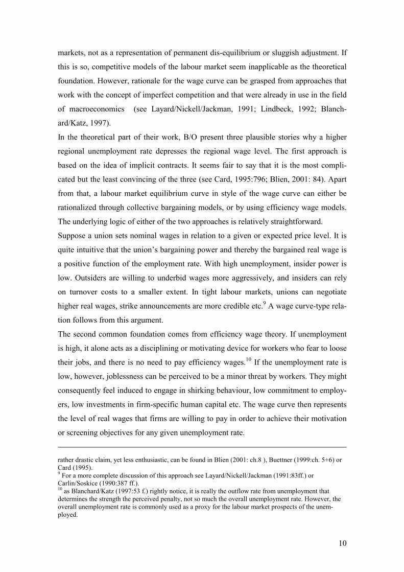
markets, not as a representation of permanent dis-equilibrium or sluggish adjustment. If

this is so, competitive models of the labour market seem inapplicable as the theoretical

foundation. However, rationale for the wage curve can be grasped from approaches that

work with the concept of imperfect competition and that were already in use in the field

of macroeconomics (see Layard/Nickell/Jackman, 1991; Lindbeck, 1992; Blanch-

ard/Katz, 1997).

In the theoretical part of their work, B/O present three plausible stories why a higher

regional unemployment rate depresses the regional wage level. The first approach is

based on the idea of implicit contracts. It seems fair to say that it is the most compli-

cated but the least convincing of the three (see Card, 1995:796; Blien, 2001: 84). Apart

from that, a labour market equilibrium curve in style of the wage curve can either be

rationalized through collective bargaining models, or by using efficiency wage models.

The underlying logic of either of the two approaches is relatively straightforward.

Suppose a union sets nominal wages in relation to a given or expected price level. It is

quite intuitive that the union’s bargaining power and thereby the bargained real wage is

a positive function of the employment rate. With high unemployment, insider power is

low. Outsiders are willing to underbid wages more aggressively, and insiders can rely

on turnover costs to a smaller extent. In tight labour markets, unions can negotiate

higher real wages, strike announcements are more credible etc.9 A wage curve-type rela-

tion follows from this argument.

The second common foundation comes from efficiency wage theory. If unemployment

is high, it alone acts as a disciplining or motivating device for workers who fear to loose

their jobs, and there is no need to pay efficiency wages.10 If the unemployment rate is

low, however, joblessness can be perceived to be a minor threat by workers. They might

consequently feel induced to engage in shirking behaviour, low commitment to employ-

ers, low investments in firm-specific human capital etc. The wage curve then represents

the level of real wages that firms are willing to pay in order to achieve their motivation

or screening objectives for any given unemployment rate.

rather drastic claim, yet less enthusiastic, can be found in Blien (2001: ch.8 ), Buettner (1999:ch. 5+6) or Card (1995). 9 For a more complete discussion of this approach see Layard/Nickell/Jackman (1991:83ff.) or Carlin/Soskice (1990:387 ff.). 10 as Blanchard/Katz (1997:53 f.) rightly notice, it is really the outflow rate from unemployment that determines the strength the perceived penalty, not so much the overall unemployment rate. However, the overall unemployment rate is commonly used as a proxy for the labour market prospects of the unem-ployed.

11

Which of the two stories is most appropriate for the purpose to address regional labour

market disparities in the European Union? It is often spelled out that union models re-

flect fairly well the institutional situation in continental Europe, whereas the efficiency

wage models apply more to the more “flexible” labour markets in the UK and the USA.

One might thus expect that a collective bargaining approach is more appropriate to ad-

dress European unemployment. However, recall that from now on we are concerned

with the regional dimension of an economy. It is true that continental European labour

markets are highly unionised. But at the same time they are characterised by a very low

degree of regional differentiation of union wages (Faini, 1999). Collective bargaining

e.g. in (West) Germany takes place at the sectoral level, but with virtually nil regional

differentiation of contracted wages.11 If at all, regional differentiation in Germany oc-

curs through differences in effective earnings, when employers consciously pay above

the union minimum wage (Suedekum, 2003b; Schnabel, 1995).

Hence, an approach that bases a wage curve on regional differences in bargaining

strength of inherently regional unions is not appropriate given the institutional structure

of most continental European labour markets. Quite contrarily, one can argue that it is

precisely because of the low degree of regional differentiation of union wages that intra-

national unemployment disparities are so evident (Suedekum, 2003b; Faini, 1999). In

the vein of the wage curve approach, efficiency wages seem to be the much more ap-

propriate micro-foundation. Regional earnings differentiation occurs, because firms

from different regions pay above the union minimum wage to a different extent. The

reasons for this positive wage drift presumably may be found in efficiency wage con-

siderations (Blien, 2001:86).

A wage curve based on efficiency wages

We will therefore use the concept of efficiency wages to provide proper micro-

foundations for the wage curve as a labour market equilibrium curve. In their mono-

graph,. B/O use a modified version of the shirking approach of Shapiro/Stiglitz (1984).

We will use an even more simplified version of the Shapiro/Stiglitz-model in this paper.

11 Formally, the regional sub organizations of the nationwide unions and employers associations bargain on the level of the German Bundesländer in most sectors. De facto, however, this hardly means anything. Typically there is one pilot agreement that is reached in one region, which subsequently is applied with-out any notable modification to all firms in that sector all over the nation (Buettner, 1999:99 ff.; Bispink, 1999), since “equal pay for equal work” in all regions is perceived to be the only socially acceptable form of wage setting.

12

We consider an economy in continuous time consisting of two regions r={1,2}, and we

assume risk-neutral workers, who gain utility from wage income wr, but disutility from

work-effort er. Utility Vr is assumed to be linear.

Vr = wr – er. (1)

Effort at work is assumed to be a technologically fixed number er > 0. Individuals can

choose to “shirk” at work and spend zero effort er=0. Shirking individuals run the risk

of being detected and then fired. The detection and firing probability (1-γr) < 1 is less

than perfect. Once fired, an individual enters the pool of the unemployed. Yet, follow-

ing Shapiro/Stiglitz (1984), there is also some exogenous destruction rate of firms Rr >

0 that likewise leads to an inflow from employment to unemployment. For simplicity,

we assume that unemployed persons have no other source of income.12

The unemployed have a chance αr of re-entering into a job. This endogenous variable

depicts the flow from unemployment back into the pool of the employed. In the steady

state equilibrium, the two labour market flows must be equal. Given that nobody will

shirk in equilibrium, we can write this condition as Rr Nr = αr (Lr-Er), where Lr is the

labour force and Er is employment. The definition of the unemployment rate is Ur = 1-

Er/Lr. This determines the function αr to be αr = (Rr / Ur) – Rr. Thus, the outflow prob-

ability from unemployment is decreasing in the regional unemployment rate Ur.

The only decision to be made by an individual is whether to shirk or not. The utility of

an unemployed individual (Vur) is given by

Vur= αr (wr – er). (2)

Non-shirking employed workers and shirkers have utility levels Venr and Vesr respec-

tively

Venr = wr – er (3)

Vesr =γr wr + (1-γr)(αr(wr - er)). (4)

The firm has an interest to prevent shirking and will thus pay efficiency wages that are

just sufficient to ensure equal utility for shirkers and non-shirkers, i.e. Vesr =Venr. Equat-

ing (3) and (4) yields after some manipulations the following expression

(1 )(1 ( ))

r rr r

r r r

ew eU

γγ α

= +− −

(5)

12 In most parts of the efficiency wage framework of B/O, they assume that regions might differ with respect to the level of unemployment benefits. We do not consider these cases, because it is irrelevant for most continental European countries. Unemployment benefits are generally not differentiated across re-

13

Equation (5) is the regional wage curve and can be interpreted as the aggregate non-

shirking condition in region r. It shows the efficiency wage that is sufficient to prevent

shirking for any given regional unemployment rate and is derived from the equilibrium

conditions in the regional labour market. Graphically, equation (5) can be represented as

in fig. 4.

Finally, we abstract from structural differences between the two single regions and as-

sume that er and γr are the same in both regions. The interpretation of this assumption

might be that there are no differences in labour market institutions. We come back to

this issue in the final section 6. This warrants that both regions face the same wage

curve locus.

The general equilibrium model of Blanchflower/Oswald

The wage curve (5) represents “one half” of the full equilibrium in the B/O-model.

More precisely it describes the labour market side of this two-region economy. The way

in which B/O (1996:77 ff.) introduce product markets to this model, i.e. the labour de-

mand side, is in fact very simple. They assume that each of the two regions produces a

distinct tradable commodity under constant returns to scale and perfect competition. The

production function for the regional tradable good Yr is given by Yr = f(Nr,Kr). Kr is

assumed to be an essential input of production for which the price i is determined on

world markets. Labour and capital in both regions have to be used in fixed proportions.

Under constant returns to scale, total minimum costs are thus simply the product of

minimum unit cost (cr) and the quantity of output Yr.

{ },

( , , ) min / / ( , )r r

r r r r r r r r r r rN KC Y w i w N Y iK Y Y c w i= + = (6)

Perfect competition and zero profits imply that cr(wr,i) need to equal the product price

pr, which is exogenous to any single firm. Without loss of generality, B/O normalize the

given product price for the good from region 1 to unity. The price of the product from

region 2 is denoted p. General equilibrium in either region is reached when product and

labour market are jointly in equilibrium. Since both regions face the same wage curve

locus, the graphical representation of the general equilibrium can be illustrated in only

one diagram, fig. 5.

gions. We therefore have assumed that unemployment benefits br are equalized on the level br=0. This normalization, however, is only for analytical simplification.

14

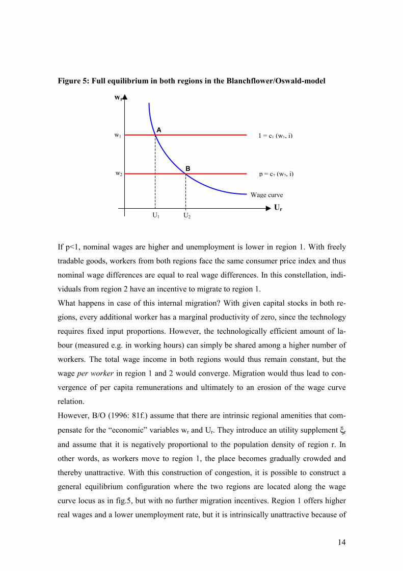
Figure 5: Full equilibrium in both regions in the Blanchflower/Oswald-model

If p<1, nominal wages are higher and unemployment is lower in region 1. With freely

tradable goods, workers from both regions face the same consumer price index and thus

nominal wage differences are equal to real wage differences. In this constellation, indi-

viduals from region 2 have an incentive to migrate to region 1.

What happens in case of this internal migration? With given capital stocks in both re-

gions, every additional worker has a marginal productivity of zero, since the technology

requires fixed input proportions. However, the technologically efficient amount of la-

bour (measured e.g. in working hours) can simply be shared among a higher number of

workers. The total wage income in both regions would thus remain constant, but the

wage per worker in region 1 and 2 would converge. Migration would thus lead to con-

vergence of per capita remunerations and ultimately to an erosion of the wage curve

relation.

However, B/O (1996: 81f.) assume that there are intrinsic regional amenities that com-

pensate for the “economic” variables wr and Ur. They introduce an utility supplement ξr

and assume that it is negatively proportional to the population density of region r. In

other words, as workers move to region 1, the place becomes gradually crowded and

thereby unattractive. With this construction of congestion, it is possible to construct a

general equilibrium configuration where the two regions are located along the wage

curve locus as in fig.5, but with no further migration incentives. Region 1 offers higher

real wages and a lower unemployment rate, but it is intrinsically unattractive because of

Bw2

U2

Wage curve

Ur

wr

w1

U1

A 1 = c1 (w1, i)

p = c2 (w2, i)

15

the regional congestion. Since the variable ξr is unobservable, there is a wage curve

visible in the data that is stable in the long run, since the regional disparities in wr and

Ur will show no tendency to vanish.

4) A critical review of the Blanchflower/Oswald-model

Several critical remarks can be made about this wage curve model, which all have to do

with the product market specification. Most importantly, the substantial origin of re-

gional differences remains an open issue. Regions are assumed to produce different fi-

nal goods and sell them at exogenous prices under perfect competition. The fact that one

region is assigned to produce a “better” good then leads to disparate regional develop-

ment.

There is an apparent identification of regions with sectors or specific products. This is

problematic for several reasons. One firstly has to take into account that regions in

Europe are far from being specialized in one or only a few products. By the same token,

specific industries are not very much concentrated in only one region. The regional con-

centration of industries might be increasing due to the process of European integration.

At the moment, however, it is certainly not high enough so as to set regions equal with

industries. Moreover, it seems to be a well established empirical fact that differences in

regional unemployment rates can only weakly be attributed to the sectoral specialization

patterns of regions.13 There rather seems to be a truly regional dimension to the problem

of spatial unemployment disparities that can not be explained by sectoral components

(see also section 2).

It is completely unspecified in the B/O-model why regions specialize in certain products

and why they do not change their specialization patterns if they see better performances

with other commodities. This complete exogeneity might not even be that critical. One

can think of model extensions where regions are characterised by different factor en-

dowments that shape the sectoral specialization through comparative cost advantages.

However, such an approach would probably still be insufficient.

The are good reasons to believe that the regional economic landscape in Europe is not

only driven by comparative advantage (Ottaviano/Puga, 1998). It was shown in section

13 See e.g. OECD (2000), R.Martin (1997), Taylor/Bradley (1983), or Elhorst (2000) (and the references therein), who concludes that “most empirical applications have indicated that spatial differences in indus-try mix account for little, if any, of the variation in unemployment rates between regions. The same indus-try seems to experience different unemployment rates in different regions.”

16

2 that the reality in the EU-15 is characterised by a clear core-periphery structure. Pro-

duction is distributed very unevenly across space, with a high degree of spatial concen-

tration of economic activity in an industrial core belt. The rich core regions clearly do

not have their status only because of underlying endowments. Instead, today’s spatial

economic configuration is also the result from endogenous cumulative processes and

circular causation mechanisms. A product market specification like in the B/O-model

can not take such processes into account.

A final critique concerns the analysis of labour mobility. In fig. 5, individuals from re-

gion 2 would want to move to region 1. But B/O assume, in an “ad-hoc” way, that re-

gional preferences are operating as an opposing factor in form of a compensating re-

gional amenity. The nasty point about this construction is that the long-run stability of

the wage curve crucially hinges on it. If the compensating amenities were not there, the

wage curve would gradually disappear.

All in all, one has to conclude that essentially everything is driven by exogenous factors

in the general equilibrium model of B/O. Regional disparities exist only by assumption.

This problem, however, can be resolved by altering the product market structure of the

model. It is necessary though to depart from the conventional framework with constant

returns and perfect competition towards an environment that works with localised in-

creasing returns to scale and imperfect competition and tradability of commodities in

spirit of the new agglomeration theories that were mentioned in the introduction. The

use of a product market structure in this vein will essentially overturn the criticism from

this section. And in fact, the case for the long-run stability of the wage curve will get

even stronger then perceived by B/O themselves.

5) Endogenous agglomeration economies

Our alternative product market specification is build around the central ideas of local-

ised increasing returns to scale and the presence of spatial transaction costs. We suppose

a two-sector model where both regions r = {1,2} produce a final consumption good Y

by assembling a variety of intermediate inputs X, which are produced and traded in both

regions. All Y-producers in both regions use all available intermediates symmetrically,

i.e. production of Y in region 1 requires both local inputs (X11) and imported inputs

(X21). Increasing returns are present in the model, because the production costs in the Y-

sector are a decreasing function of the number of available industrial intermediates from

either region (Nr). This argument for increasing returns, the expansion of the variety of

17

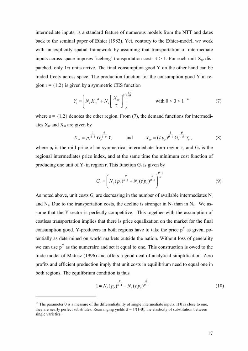
intermediate inputs, is a standard feature of numerous models from the NTT and dates

back to the seminal paper of Ethier (1982). Yet, contrary to the Ethier-model, we work

with an explicitly spatial framework by assuming that transportation of intermediate

inputs across space imposes ´iceberg´ transportation costs τ > 1. For each unit Xsr dis-

patched, only 1/τ units arrive. The final consumption good Y on the other hand can be

traded freely across space. The production function for the consumption good Y in re-

gion r = {1,2} is given by a symmetric CES function

1

srr r rr s

XY N X Nθ θ

θ

τ = +

with 0 < θ < 1 14 (7)

where s = {1,2} denotes the other region. From (7), the demand functions for intermedi-

ates Xrr and Xsr are given by

1

1 1rr r r rX p G Y

θθ θ− −= and

11 1( )sr s r rX p G Y

θθ θτ − −= , (8)

where pr is the mill price of an symmetrical intermediate from region r, and Gr is the

regional intermediates price index, and at the same time the minimum cost function of

producing one unit of Yr in region r. This function Gr is given by

1

1 1( ) ( )r r r s sG N p N p

θθ θ θ

θ θτ

−

− −

= +

(9)

As noted above, unit costs Gr are decreasing in the number of available intermediates Nr

and Ns. Due to the transportation costs, the decline is stronger in Nr than in Ns. We as-

sume that the Y-sector is perfectly competitive. This together with the assumption of

costless transportation implies that there is price equalization on the market for the final

consumption good. Y-producers in both regions have to take the price pY as given, po-

tentially as determined on world markets outside the nation. Without loss of generality

we can use pY as the numeraire and set it equal to one. This construction is owed to the

trade model of Matusz (1996) and offers a good deal of analytical simplification. Zero

profits and efficient production imply that unit costs in equilibrium need to equal one in

both regions. The equilibrium condition is thus

1 11 ( ) ( )r r s sN p N pθ θ

θ θτ− −= + (10)

14 The parameter θ is a measure of the differentiability of single intermediate inputs. If θ is close to one, they are nearly perfect substitutes. Rearranging yields σ = 1/(1-θ), the elasticity of substitution between single varieties.

18

In both regions, each of the single intermediates is produced by using labour only. The

labour requirement � necessary to produce the quantity X is given by

� = α + βX with α>0, β>0 (11)

Due to the fixed costs α, and the unlimited number of potential varieties in the X-sector,

every single intermediate will be produced by only one firm. Each firm from region r

sells its distinct product X at price pr. Following Dixit/Stiglitz (1977) we say that single

producers are small relative to the market. This implies that profit maximizing prices are

a constant mark-up over marginal costs, which are constituted solely by the wage costs

wr.

r rp wβθ

= (12)

Furthermore, profits for every single intermediate good are driven down to zero by the

entry of potential competitors. This implies that all X-firm, regardless of their location,

are operating at the same scale of output (13), which requires an exactly determined

amount of labour per firm (14).

−

=

θθ

βα

1X (13)

and θ

α−

=1

� (14)

The maximum number of intermediates that a region can potentially produce is re-

stricted by labour supply rL if the labour is fully employed. If a fraction Ur of the la-

bour force is unemployed, the equilibrium number of firms is by definition

(1 ) rr r

LN U= −�

(15)

The higher is employment in region r, the more firms are active in that region, and the

cheaper is Y-production in both regions, but particularly in the region r itself.

Equilibrium

With costless trade (τ = 1), it would not matter where intermediates are produced, since

they are equally available everywhere. As shown by Matusz (1996), regional wages

19

would be equalised at ( )( )(1 )1 2 1 2w w N N θ θθ β −= = + .15 With transportation costs τ >1,

however, the larger region has an advantage over the smaller one since it can produce

more intermediates locally. Consequently, regional wage equalization does not occur if

the regions differ in size, but the larger region pays an agglomeration wage premium.

By substituting (15) and (12) into (10), where we have set β=θ for simplicity, we obtain

for region r =1.

1

11

12 1

2 2

(1 )

1 (1 ) ( )

LUw

LU w

θθ

θθτ

−

−

−

= − −

�

�

(16)

The nominal (=real) regional wage w1 is increasing in employment in both regions, but

decreases with higher wages in region 2 and transportation costs τ. An analogous equa-

tion applies to region s = {1,2}. Solving for w1 and w2, we can obtain closed-form solu-

tions for the regional equilibrium wages 1

11 1(1 ) Lw T U

θθ−

= − �

,

1

22 2(1 ) Lw T U

θθ−

= − �

(17)

where 1

12

1

1

−

−

−

−=θθ

θθ

τ

τT

At these wage levels, there is profit maximization and zero profits in both sectors and

both regions. As can be seen, the equilibrium levels of w1 and w2 only depend (posi-

tively) on employment in the respective region itself. E.g., an increase in L2 only has

positive effects on the wage in region 2, but not in region 1. This is due to the symmet-

rical use of all intermediates in both regions. An increase in L2 has at first instance also

positive spillover effects in region 1. But once the endogenous effect on w2 is taken into

account, the impact will cancel out. Economically, (17) implies that the model incorpo-

rates a purely regional scale externality. A larger labour force in region 2 implies higher

equilibrium wages in that region due to the better exploitation of localised scale econo-

mies. But despite the openness, there are effectively no interregional spillovers of any

type. It is also noteworthy that w1 and w2 decrease proportionally with the higher trans-

15 This result is one central insight of the ´new trade theory´ in spirit of Ethier (1982), namely that inter-mediates production does not need to be spatially concentrated, but that the exploitation of increasing returns can be “international”.

20

portation costs τ. The variable T can be understood as an inverse measure of the re-

source waste from shipping and ranges between T = 1 (if τ→ ∞), and T=2

(if τ → 1). Formally, the regional wages in (17) are consistent with efficient production

in the Y- and X-sectors in both regions. But moreover, they also imply clearing of all

markets in this economy. The wages w1 and w2 from (17) are thus the true equilibrium

wages. This proposition is proofed in the appendix.

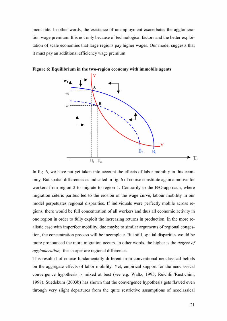
Graphically, (17) is represented by the curves B1B1 and B2B2 in fig. 6. The product

market equilibrium curves are no longer horizontal lines as in the B/O-model (fig. 5),

but are now downward sloping curves due to localised internal increasing returns. For

any given unemployment rate, the region with the larger labour force (r=1) pays the

higher equilibrium real wage. The intuition for this scale effect is straightforward. Re-

gion 1 produces more local intermediate goods than region 2, since total employment is

higher. Region 1 thus saves on transportation costs. It must consequently pay higher

wages for the zero profit conditions in the Y- and the X-sector to hold. Hence, for all

points below a BB-schedule, wages are too low for a given unemployment rate. This

determines the vertical phase arrows. The higher is the difference between L1 and L2,

the further apart are B1B1 and B2B2. An increase in τ shifts both curves downwards and

to the left, because the dead weight loss of resources wasted in transportation increases.

The same shift occurs as α, β, or θ increase.

Full equilibrium is reached if both product and labour markets are jointly in equilib-

rium. Equilibrium in the labour market is represented by the wage curve VV in fig.6,

which is given by equation (5) and identical to the wage curve from fig. 5. For all points

to the right of VV, unemployment is too high for any given wage. Consequently firms

can hire new workers and trust that they do not shirk. Equilibrium unemployment must

fall.

The stable equilibrium points are at A and B respectively. As can be seen, region 1 has

both the higher equilibrium wage and the lower unemployment rate. Recall that we have

assumed that region 1 is larger than region 2, and can therefore better exploit the scale

economies. The labour demand consistent with product market equilibrium is higher in

region 1 for any given wage rate. This drives down unemployment at first instance and

simultaneously increases the necessity to pay efficiency wages in order to prevent indi-

viduals from shirking. In equilibrium, the larger region (“the core”) is advantaged over

the smaller one along two dimensions: by having higher wages and a lower unemploy-

21

ment rate. In other words, the existence of unemployment exacerbates the agglomera-

tion wage premium. It is not only because of technological factors and the better exploi-

tation of scale economies that large regions pay higher wages. Our model suggests that

it must pay an additional efficiency wage premium.

Figure 6: Equilibrium in the two-region economy with immobile agents

In fig. 6, we have not yet taken into account the effects of labor mobility in this econ-

omy. But spatial differences as indicated in fig. 6 of course constitute again a motive for

workers from region 2 to migrate to region 1. Contrarily to the B/O-approach, where

migration ceteris paribus led to the erosion of the wage curve, labour mobility in our

model perpetuates regional disparities. If individuals were perfectly mobile across re-

gions, there would be full concentration of all workers and thus all economic activity in

one region in order to fully exploit the increasing returns in production. In the more re-

alistic case with imperfect mobility, due maybe to similar arguments of regional conges-

tion, the concentration process will be incomplete. But still, spatial disparities would be

more pronounced the more migration occurs. In other words, the higher is the degree of

agglomeration, the sharper are regional differences.

This result if of course fundamentally different from conventional neoclassical beliefs

on the aggregate effects of labor mobility. Yet, empirical support for the neoclassical

convergence hypothesis is mixed at best (see e.g. Waltz, 1995; Reichlin/Rustichini,

1998). Suedekum (2003b) has shown that the convergence hypothesis gets flawed even

through very slight departures from the quite restrictive assumptions of neoclassical

V

U2U1

Bw2

B2

wr

w1

A

B1

V

Ur

22

models. For our purpose, it is most important to stress one essential point: if labour mi-

gration spurs regional divergence, this implies that the wage curve is a stable interre-

gional relation with no tendency of erosion.

6) Discussion and concluding remarks

In section 4, we have pointed out some fundamental criticisms with respect to the wage

curve model of B/O. In short, we have criticised: (a) that regional disparities can not

develop endogenously, but must be due to exogenous assumptions, (b) that regions were

essentially identified with sectors, (c) that the B/O-models is not able to explain re-

gional agglomeration, even tough it is the most salient features of the European eco-

nomic landscape, and (d) that labour mobility leads to an erosion of the wage curve, so

that the long-run stability critically hinges on restrictive ad-hoc assumptions.

Our alternative approach from section 5 leads to different conclusions with respect to all

these four points. Since we have incorporated a scale effect in the production function,

we have taken into account an endogenous mechanism for regional disparities to de-

velop, namely the presence of localised increasing returns to scale. Sectoral specializa-

tion patterns play no critical role in our model. Both locations are engaged in production

activities within the same sectors. Differences in the production structure exist insofar

that the larger region can produce a higher number of industrial intermediates. But all

regional differentiation, and all interregional trade, is of an intra-industry type. Lastly,

the wage curve is not put under strain by labour mobility as in the B/O-model, but rather

strengthened by it. Hence, if one works with an increasing returns technology, the theo-

retical case for the existence of a wage curve is even stronger than it has been argued by

B/O themselves. No “ad-hoc” construction of compensating regional amenities is

needed to warrant the long-run stability of the wage curve.

The contribution of our paper, however, can also be interpreted differently, namely as

an attempt to integrate the element of unemployment to the new regional agglomeration

theories. We have argued in the introduction that the literature in NEG and NTT is

vastly growing, yet mostly silent about unemployment disparities. Our model is an at-

tempt to partly close this gap. It is not strictly a NEG-model, effectively because the

analysis is not about the trade-off between centripetal and centrifugal forces to shape an

economic landscape. It is actually closer to models of the NTT (Ethier, 1982; Matusz,

1996). But contrarily to this literature, our model is an explicitly regional approach, as it

takes into account spatial transaction costs and the effects of labour mobility.

23

The important result of our paper is that the large core region, where workers and pro-

duction are agglomerated, will exhibit a lower unemployment rate than the sparsely

populated peripheral region, and the core will pay a real wage premium. This result is

consistent with the stylised facts about the geographical structure of economic activity

in the EU-15. In section 2 we have shown that regional unemployment rates follow a

trans-national core-periphery-structure that resembles the spatial configuration of GDP

per capita. Low unemployment is centred in the agglomeration area (the “European Ba-

nana”), whereas the poor “objective 1”-regions mostly have very high unemployment

rates. Moreover, we have shown that the spatial structure of joblessness today is the

result of a polarisation process of regional unemployment rates that was mainly driven

by the labour demand side. Densely populated and rich regions on average received

immigrants, but experienced falling unemployment rates. The opposite happened in the

already poor and sparsely populated sending regions.

These stylised facts can be understood with our theoretical model. The immigration of

additional workers to the core regions does not primarily cause an increase of competi-

tion on the labour supply side. There are stronger secondary effects on the labour de-

mand side, caused by the better exploitation of scale economies, that lead to higher

wages and lower unemployment in the centre. All in all, we conclude that our model

approach is not only an innovation from the theoretical point of view, but also is of em-

pirical relevance.

As a final point, we want to discuss the issue of inter- versus intra-national unemploy-

ment disparities and the role of labour market institutions for determining regional un-

employment rates. Recall that we have assumed in section 3 that the parameters er and γr

in the partial model of the labour market equilibrium curve are identical in both regions.

The interpretation of this assumption, that warranted that the wage curve locus VV in

fig. 6 is the same in both regions, could be that there is no regional variation in labour

market institutions. One could easily think of model extensions where the parameters er

and γr reflect structural characteristics of the respective labour market. The firing prob-

ability γr might e.g. be influenced by employment protection laws, or the work effort

parameter er is a reservation wage dependent on welfare state arrangements etc.

The assumption identical institutions in the two regions restricts the applicability of our

model at first instance to the case of intra-national unemployment disparities. Within the

same country, there is typically very little institutional variation across regions. E.g.,

24

labour laws, welfare state arrangements, the tax regime etc. are typically valid nation-

wide. In other words, for the case of intra-national unemployment disparities, it seems

reasonable to assume that all regions face the same wage curve locus. We have seen in

figure 1 that the same set of (national) labour market institutions still can bring about

utterly different unemployment rates on the regional level. Our model helps to explain

this puzzle, since it suggests that unemployment disparities are mainly driven by re-

gional economic agglomeration.

Nevertheless, our interest was not constrained to the case of intra-national differences.

Our model is also applicable to understand the spatial structure of unemployment in the

EU-area as a whole. Across the single EU-member countries, however, there is still a

notable degree of variation in labour market institutions. Regions from France might

e.g. face a different wage curve locus than regions from Germany or Spain. For the case

of labour market disparities of regions that belong to different countries, we can thus no

longer assume that they face the same VV-locus. The observed regional differences in

this case are a combination of institutional differences (VV-curves) and the degree of

agglomeration (BB-curves).

The fact that national borders play only a minor role as division lines of the three trans-

national unemployment clusters in the EU-15 (map 1) suggests that the actual influence

of labour market institutions for determining unemployment might be smaller than it is

frequently stressed in many academic and popular discussions. But labour market insti-

tutions are not irrelevant. The Portuguese regions are a good example for this claim.

They all belong to the “objective 1”-cluster, but still unemployment rates are relatively

low. This is supposedly so, because Portugal has at least in some respects a set of fa-

vourable institutions, i.e. a wage curve VV that is located closer to the origin as in other

nations.16

To sum up, the regional labour market disparities, or more generally the spatial structure

of unemployment in the EU-15, is determined by an interplay of (national) institutions

and the degree of regional agglomeration. The influence of the latter seems to be

greater. On a regional level, high unemployment seems to result primarily because of

economic peripherality and a low degree of agglomeration. It seems not so much to be

caused by unfavourable labour market institutions, since in many cases other regions

16 For a more detailed discussion about the particularities of the Portuguese labour market see Addi-son/Texeira (2001) or Bover/Garcia-Perea/Portugal (2000).

25

from the same country demonstrate that very low regional unemployment rates are very

well consistent with the same institutional frame.

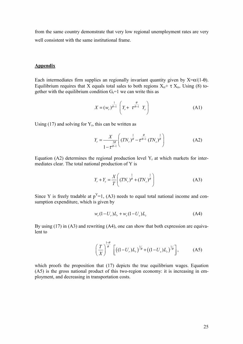
Appendix

Each intermediates firm supplies an regionally invariant quantity given by X=α/(1-θ). Equilibrium requires that X equals total sales to both regions Xrr+ τ Xrs. Using (8) to-gether with the equilibrium condition Gr=1 we can write this as

1

1 1( )r r sX w Y Yθ

θ θτ− −

= +

(A1)

Using (17) and solving for Yr, this can be written as

1 1

12

1

( ) ( )1

r r sXY TN TN

θθ θ θ

θθ

ττ

−

−

= −

− (A2)

Equation (A2) determines the regional production level Yr at which markets for inter-mediates clear. The total national production of Y is

1 1

( ) ( )r s r sXY Y TN TNT

θ θ

+ = +

(A3)

Since Y is freely tradable at pY=1, (A3) needs to equal total national income and con-sumption expenditure, which is given by (1 ) (1 )r r r s s sw U L w U L− + − (A4) By using (17) in (A3) and rewriting (A4), one can show that both expression are equiva-lent to

( ) ( )1

1 1(1 ) (1 )r r s s

T U L U LX

θθ

θ θ

−

− + − , (A5)

which proofs the proposition that (17) depicts the true equilibrium wages. Equation (A5) is the gross national product of this two-region economy: it is increasing in em-ployment, and decreasing in transportation costs.

26

References Addison, J.T., P. Teixeira (2001) “Employment Adjustment in a Sclerotic Labor Mar-ket: Comparing Portugal with Germany, Spain, and the United Kingdow”, Jahrbuecher fuer Nationaloekonomie und Statistik 221 (4): 353-370. Bispink, R. (1999) “Tarifpolitik und Lohnbildung in Deutschland am Beispiel ausge-wählter Wirtschaftszweige“, WSI Discussion Papers 80, Duesseldorf. Blanchard, O., L. Katz (1997) “ What We Know and Do not Know about the Natural Rate of Unemployment”, Journal of Economic Perspectives 11: 51-72. Blanchflower, D., A. Oswald (1996), The Wage Curve, Cambrige (Mass.): MIT Press. Blanchflower, D., A. Oswald (1994) “An Introduction to the Wage Curve”, (mimeo), University College London. Blanchflower, D., A. Oswald (1990) “The Wage Curve”, Scandinavian Journal of Eco-nomics 92: 215-235. Blien, U. (2001), Arbeitslosigkeit und Entlohnung auf regionalen Arbeitsmärkten, Hei-delberg, New York: Physica. Bover, O., P. Garcia-Perea, P. Portugal (2000) “Labour market outliers: Lessons from Portugal and Spain”, Economic Policy 15, no. 31: 379-428. Buettner, T. (1999), Agglomeration, Growth, and Adjustment, ZEW Economic Studies, Heidelberg, New York: Physica. Card, D. (1995) “The Wage Curve: A Review”, Journal of Economic Literature 33: 785-799. Carlin, W., D. Soskice (1990), Macroeconomics and the Wage Bargain. A Modern Ap-proach to Employment, Inflation and the Exchange Rate, Oxford: Oxford University Press. CER (1998) “Il lavaro negli anii dell´Euro”, Rapporto CER 3, Milano. Dixit, A., J. Stiglitz (1977) “Monopolistic Competition and Optimum Product Diver-sity”, American Economic Review 67: 297-308. Elhorst, J.P. (2000) “The Mystery of Regional Unemployment Differentials: A Survey of Theoretical and Empirical Explanations”, University of Groningen Working Papers. Ethier, W. (1982) “National and International Returns to Scale in the Modern Theory of International Trade”, American Economic Review 72: 389-405.

27

European Commission (2001), Second Report on Economic and Social Cohesion, Brus-sels. available under: http://europa.eu.int/comm/regional_policy/sources/docoffic/official/reports/contentpdf_en.htm Faini, R. (1999) “Trade Unions and Regional Development”, European Economic Re-view 43: 457-474. Fuhita, M., P. Krugman, A. Venables (1999), The Spatial Economy: Cities, Regions, and International Trade, Cambridge (Mass.): MIT Press. Hall, R. (1970) “Why is the Unemployment Rate so High at Full Employment?”, Brookings Papers on Economic Activity 3: 369-402. Hall, R. (1972) “Turnover in the Labor Force”, Brookings Papers on Economic Activity 3: 709-756. Harris, J., M. Todaro (1970) “Migration, Unemployment and Development: A Two-Sector Analysis”, American Economic Review 60: 126-142. Hughes, G., B. McCormick (1985) “Migration Intentions in the U.K. – Which House-holds Want to Migrate and Which Succeed?” Economic Journal 95:113-123, Confer-ence Papers Supplement Krugman, P. (1991) “Increasing Returns and Economic Geography”, Journal of Politi-cal Economy 99: 483-499. Krugman, P. (1980) “Scale Economics, Product Differentiation, and the Pattern of Trade”, American Economic Review 70: 950-959. Layard, R., S. Nickell, R. Jackman (1991), Unemployment: Macroeconomic Perform-ance and the Labor Market, Oxford: Oxford University Press. Lindbeck, A. (1992) “Macroeconomic Theory and the Labour Market”, European Eco-nomic Review 36: 209-235. Martin, R. (1997) “Regional Unemployment Disparities and their Dynamics”, Regional Studies 31: 237-252. Martin, R., P. Tyler (2000) “Regional Employment Evolutions in the European Union: A Preliminary Analysis”, Regional Studies 34: 601-616. Matusz, S. (1996) “International trade, the division of labour, and unemployment”, In-ternational Economic Review 37: 71-84. Mincer, J. (1974), Schooling, Experience, and Earnings, New York: Columbia Univer-sity Press. OECD (2000) “Disparities in Regional Labour Markets”, OECD Employment Outlook Paris, p. 31-78.

28

Ottaviano, G., D. Puga (1998) “Agglomeration in the Global Economy: A Survey of the ´New Economic Geography´”, World Economy 21: 707-731. Overman, H., D. Puga (2002) “Unemployment Clusters across European Regions and Countries”, Economic Policy, no.34:115-147. Partridge, M., D. Rickman (1997) “Has the Wage Curve Nullified the Harris-Todaro Model? Further US Evidence”, Economics Letters 54: 277-282. Peeters, J., H. Garretsen (2000) “Globalisation, Wages and Unemployment: An Eco-nomic Geography Perspective”, CESifo Working Paper 256, Munich. Puga, D. (2002) “European Regional Policies in Light of Recent Location Theories”, Journal of Economic Geography 2: 302-334. Reichlin, P., A. Rustichini (1998) “Diverging Patterns with Endogenous Labor Migra-tion”, Journal of Economic Dynamics and Control 22: 703-728. Schnabel, C. (1995) “Übertarifliche Entlohnung: Einige Erkenntnisse auf Basis betrieb-licher Effektivlohnstatistiken“, in: Gerlach, K., R. Schettkat (eds.), Determinanten der Lohnbildung, Berlin: Ed. Sigma. Shapiro, C., J. Stiglitz (1984) “Equilibrium Unemployment as a Worker Discipline De-vice”, American Economic Review 73: 433-444. Suedekum, J. (2003a), Agglomeration and Regional Unemployment Disparities, PhD thesis, Goettingen University. Suedekum, J. (2003b) “Selective Migration, Union Wage Setting, and Unemployment Disparities in West Germany”, (forthcoming) International Economic Journal. Taylor, J., S. Bradley (1983) “Spatial Variations in the Unemployment Rate: A Case Study of North-West England”, Regional Studies 17: 113-124. Walz, U. (1995) “Growth (Rate) Effects of Migration“, Zeitschrift fuer Wirtschafts- und Sozialwissenschaft 115: 199-221.

Guyane (F)

Guadeloupe

(F)

Martinique

(F)

Réunion

(F)

Canarias (E)

Açores (P)

Madeira

(P)

Kypros

< 4.95

4.95 - 7.85

7.85 - 10.75

10.75 - 13.65

>= 13.650 km100 500

gRe oi GISge oi GISR

% of labour force

EUR-27 = 9.3Standard deviation = 5.74

Sources: Eurostat and NSI

© EuroGeographics Association for the administrative boundaries

Map 1: Unemployment rate by region, 2000

Guyane (F)

Guadeloupe

(F)

Martinique

(F)

Réunion

(F)

Canarias (E)

Açores (P)

Madeira

(P)

Kypros

< 30

30 - 50

50 - 75

75 - 100

100 - 125

>= 1250 km100 500

gRe oi GISge oi GISR

Index, EUR-27 = 100

Source: Eurostat

© EuroGeographics Association for the administrative boundaries

Map 2: GDP per head by region (PPS), 1999