PROCESS CONTROL AND INFORMATION SYSTEMS SPECIALREPORT

Increase your margin by 25%Here's how to make sure that the planning LPs always match the plant

A. BEERBAUM, Chevron, San Ramon, California; W. KORCHINSKI,Advanced Industrial Modeling Inc., Santa Barbara, California; andD. GEDDES, PREPConsulting Inc., Denver, Colorado

Intoday's over-constrained work environment, planning modelaccuracy does not get the attention it deserves. In this article,we discuss order-of-magnitude LP (planning linear program)

errors, what effect they have on margins and how to improveyour LPs.

Oil refiners and petrochemical plant operators plan and opti-mize their operations using LPs. Typical uses for planning LPsinclude crude oil/feedstock selection, production planning andmonthly shutdown planning. Despite the fact that LPs have beenin use for more than 40 years, and that major improvements havebeen made in their numerical techniques, 1 it is difficult to keepthem running accurately-mainly because of the complexity ofthe process facilities they are used to model.

Getting LPs accurate and keeping them that way is valuable.A 2004 NPRA Annual Meeting paper presented by SolomonAssociates documents the value of planning model accuracy (Table1).2 Applying a midrange value of 0.50 $/bbl from Table 1 to a300-thousand-bpd refinery results in a savings of over $50 millionper year. This figure is large because in many cases involving crudeoil selection and monthly plans, errors in the planning model leaddirectly to incorrect economic decisions.

Because of these large benefits, industry best practice is to con-tinuously monitor plant yields, compare them to planning processmodel yields and update the planning process unit models whennecessary. It is common for these updates to occur every three tofourmonths. These frequent updates help leading refiners and petro-chemical operators to squeeze more profit from their assets.

This article explores planning LP accuracy best practices. Wewill review the kinds of planning model errors found in practice,and how an inaccurate LP negatively impacts a company's margin.We will also look at how individual planners can keep their LPsrunning in top condition.

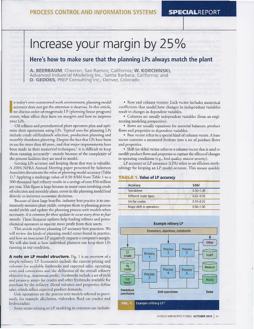
A note on LP model structure. Fig. 1 is an overview of asimple refinery LP. Economics include the current pricing andvolumes for available feedstocks and expected sales, operatingcosts and constraints and the definition of the overall refineryobjective (e.g., maximum profit). Feedstocks include a set of yieldand property assays for crudes and other feedstocks available forpurchase by the refinery. Blend volumes and properties definesales, which reflect expected product demands.

Unit operations are the process unit models referred to previ-ously, for example alkylation, visbreaker, fluid cat cracker andhydro cracker.

Some terms relating to LP modeling in common use include:

• Rowand column vectors: Each vector includes numericalcoefficients that model how changes in independent variablesresult in changes in dependent variables.

• Columns are usually independent variables (from an engi-neering modeling perspective).

• Rows are usually equations for material balances, productflows and properties or dependent variables.

• Base vector refers to a special kind of column vector. A basevector converts a measured feedrate into a set of product flowsand properties.

• Shift (or delta) vector refers to a column vector that is used tomodify product flows and properties to capture the effects of changesin operating conditions (e.g., feed quality, reactor severity).

LP accuracy or LP assurance (LPA) refers to an efficient meth-odology for keeping an LP model accurate. This means quickly

TABLE 1. Value of LP accuracyAccuracy $/bbl

Standalone 0.50-1.00

Different crude types 0.25-0.50

Similar crudes 0.10-0.25

Major shift in operations 0.50-1.00

Example refinery lP

Economics, objectives, constraints

Process ProcessProcess 3 5

1

Process Process4 6

Feedstockpurchases Unit operations Sales

Example refinery LP.3

HYDROCARBON PROCESSING OCTOBER 2010 I 41

SPECIALREPORT PROCESS CONTROL AND INFORMATION SYSTEMS

comparing the LP predictions (0 actual plant operation over timeand quickly improving the predictions.

lP prediction errors. Refinery planning LP models approxi-mate the steadystate behavior of actual operation. A refinery LPmodel comains many discrete modeling blocks ("unit models" or"submodels"), where each block represems a single process unit inme refinery. Examples of unit models are crude units, fluid catalyticcrackers, hydro crackers and so on. The LP's unit models processcrude the same way the process units in a refinery process crude.

When first built, planning LPs generally match the plant oper-arion well. However, like everything else, LPs age, and as theydo, their abiliry (0 match actual operation falls off. With time,unit model predictions deviate further from real operation, Eq. 1defines LP error over rime:

100 ~ (LP Prediction; - Measurement; )Percent error = -- L...

N ;=1 Measurement;

Where:Percent error = Error between a predicted value and the plant(e.g., for gasoline)i = Sample numberN = Number of samples over time periodLP prediction; = LP unit model prediction at each point i intime (e.g., for gasoline in bpd)

Measurement; = Measured value at each point i in time (e.g.,for gasoline in bpd)

Gasoline

Six months

LP prediction error (gasoline example).

LPG

~~------~~--~---+--~I-----1

Six months

LP prediction error (LPG example).

42 I OCTOBER 2010 HYDROCARBON PROCESSING

(1)

lP prediction error defined. How do LP predictions lookin practice? Fig. 2 shows an example for gasoline. The blue line isthe measured gasoline flow over a six-month period. The red lineis the prediction from the LP over the same period. The greenline is me LP prediction from a well-tuned LP unit model (moreabout this later).

Fig. 3 shows similar results for propane. Two observations areimportant. First, the LP errors are quite large (red line compared(0 blue line). This means that me LP is not modeling plant behav-ior accurately. The consequence of inaccurate predictions likethis is that the refinery will not be run optimally, which is veryexpensive. W~ discuss this in more detail later. Second, adjustingthe coefficients improves the LP unit model enabling it matchthe plant very well (green line). The coefficient adjustment steprequires care. For example, treating me coefficient-fitting problemas a statistical fit over a range of data, rather than at a single pointenormously improves results.

Fig. 4 shows prediction errors for a number of familiar refinerystreams. Each of the bars in Fig. 4 represems the error for a par-ticular stream averaged over one year for a number of refineries.The taller bars (labeled "Base LP") are me average errors from meLP that was in use at the time the analysis was done. The shorterbars (labeled "Improved LP") represent the relative improve-ments made after adjusting the LP coefficients. In many cases, theimproved LP errors are half as large as the base errors.

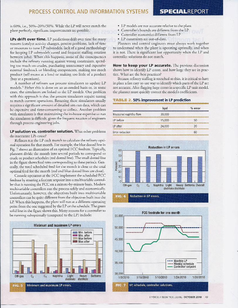
Fig. 5 shows the minimum and maximum LP prediction errorfor each of the refinery streams. "Before" and "After" refer (0 theLP before and after it was improved. Neither the minimum northe maximum errors are all from a single refinery; that is eachrefinery included some streams that had low LP prediction errors,as well as other streams that had high LP prediction errors. Themaximum LP errors were dramatically smaller after the LPs wereimproved. In most cases, the minimum LP errors are also smallerafter improving the LP.

Fig. 6 summarizes the improvement in overall LP predictionmade by adjusting me coefficients (0 match plant operation overone-year. For most streams, the improvement is between 40%and 50%.

To put this kind of improvement in perspective, Table 2 showsan example of what a 60% improvement means. The naphtha flow"before" improving me LP is 15,000. Since, this is half of me mea-sured flow of30,000 bpd, me "before" error is 50%. The naphthaflow "after" improving the LP is 24,000, which is now only a 20%error compared (0 me measured naphtha flow. The error reduction

Average LP errors

c::3 Base LPI---------.j _Improved LP

Offgas Naphtha Light Heavy Bottomsdistillate distillate

Average LP errors.

SPECIALREPORTPROCESS CONTROL AND INFORMATION SYSTEMS

is 60%, i.e., 50%-20%/50%. While the LP will never match theplant perfectly, significant improvements are possible.

LPsdrift over time. LP predictions drift over time for manyreasons (catalyst activity changes, process problems, lack of timeor resources to tune LP submodels, lack of a good methodologyfor keeping LP submodels tuned and frequent staffing rotationbetween jobs). When this happens, some of the consequencesinclude the refinery running against wrong constraints, spend-ing too much on crudes, purchasing unnecessary and expensiveexternal feedstock or blending components, making too muchproduct (sell excess at a loss) or making too little of a product(buy at a premium).

A number of refiners use process simulators to update LPmodels." Either this is done on an as-needed basis or, in somecases, the simulators are linked to the LP models. One problemwith this approach is that the process simulators require tuningto match current operations. Retuning these simulators usuallyrequires a significant amount of detailed test-run data, which canbe expensive and time-consuming to collect. Another problemwith simulators is that maintaining the in-house expertise to runthe simulators is difficult, given the frequent rotation of engineers'through process engineering jobs.

LPsolution vs. controller solution. What other problemsdo inaccurate LPs cause?

Refiners run the LP each month to calculate the refinery opti-mal operation for that month. For example, the blue dotted line inFig. 7 shows an illustration of an optimal FCC feedrate. Typically,planners divide the month into several periods to correspond tocrude or product schedules (red dotted line). The small dotted linein the figure shows 'feed rates corresponding to these periods. Gen-erally, the total scheduled feed for the month is close to the totaloptimal feed for the month (red and blue dotted lines are close).

Console operators at the FCC implement the scheduled FCCfeedrate by entering a feedrate setpoint into a multivariable control-ler that is running the FCC on a minute-by-minute basis. Modernmultivariable controllers run the process safely and economically.Unfortunately, however, the objectives built into multivariablecontrollers can be quite different from the objectives built into theLP. When this happens, the plant will run at a different operatingpoint from the one suggested by the LP or the schedule. The greensolid line in the figure shows this. Many reasons for a controller tobe running suboptimally (compared to the LP) include:

Minimum and maximum LP errors

I:'ZB Min. beforef-------------j 1----1 •• Min. after

CJ Max beforef------I f-------j f----/ ilia!Max after

Off-gas Naphtha Light Heavydistillate distillate

Minimum and maximum LP errors.

• LP models are not accurate relative to the plant• Controller's bounds are different from the LP• Controller economics different from LP• LP constraints are out-of-date.Planners and control engineers must always work together

to understand when the plant is operating optimally, and whenit is not. There is significant lost opportunity when the LP andcontroller solutions do not match.

How to keep your LP accurate. The previous discussionshows how to identify LP errors, and how large they are in prac-tice. What are the best practices?

Because refinery staffing is stretched so thin, it is critical to havein place a fast easy-to-use way to identify which parts of the LP arenot accurate. After flagging large errors in a specific LP unit model,the planner must quickly correct the model's coefficients.

TABLE 2. 50% improvement in LP prediction

bpd % error

Measured naphtha flow 30,000

LP before 15,000 50

LPafter 24,000 20

Error reduction 60

Reduction in LP errors60

50_ 40c:~30'"Co. 20

~1[" h iJ ~ =

i-il m ,

rr ',' '" ""' i(,,-.-

.. -:' ; m; ;;. I::: I'IL,,'I) ..~ i;;~! i?e t~;I I I I I I I

10

oOff-gas C3 C4 Naphtha Light Heavy Bottoms Overall

distillate distillate

Reduction in LP errors.

FCC feed rate for one month55,000,--------------------,

................50,000 ~-~-i-/_~---.,~...~~S;;~~--~

:.................45,000I-------~I-------------j

40,000I--~...I---------------I

35,0001-----------/

30,000L- ...l,..- -L --L. --L...J

1/3/2010 1/10/2010 1/10/2010 1/31/20101/24/2010

Lp, schedule, controller solutions.

HYDROCARBON PROCESSING OCTOBER 2010 I 43

SPECIALREPORT PROCESS CONTROL AND INFORMATION SYSTEMS

The workflow is:• Get unit model from LP into LP assurance tool.• Collect plant data.• Validate plant data.• Measure LP unit model accuracy.• Then, for unit models which have large errors:

o Calculate new submodel coefficients.o Validate accuracy of new coefficients.o Get improved coefficients back into LP model.o Test new coefficients.

This entire process should only take a few minutes of a planner's orprocess engineer's time.

Historic refining margins. How do we translate the prob-lems caused by LP errors into economic terrnsf

To get some perspective, let's look at historic refining margins(Fig. 8). Refining margins represent the profitability for runninga refinery-the more positive the number, the more profitablethe refinery. Recognizing that each refinery in the world has its

Worldwide average refining margin12.--------------------------------------,

10

8~----------------~--------~~--+_-----16~--------------------------~~._H_--~-1

-4L-~--~------~------~----~L-----~--~Sep-94 Sep-05Jun-97 Mar-OO Dec-02 Jun-08

Worldwide refining rnarqin.>

Assemble LP Pricing, crude Make monthly Monthlyinputs - availability, - LP run - plandemands ... (0.39 $/bbl)

I+

Buy crudes, Production Run process Controller- - setpointsfeedstocks schedule units (0.12 $/bbl)

I+

Make blends r-- Finished f--- Ship and sell f--- Revenueproducts products

I+

Financial f--- Refineryaccounting margin

From LP inputs to refining margin.

46 I OCTOBER 2010 HYDROCARBON PROCESSING

own specific margin (based on geography, plant configurationand feedstocks), we will use the average margin shown in Fig.8 to illustrate how a more accurate planning LP translates intoan improved margin. Notice that recently refining margins havedeclined rather dramatically. In the economic analysis that follows,we will use a historically representative refining margin.

Improve LP, improve corporate margin. There aremany ways to use planning LPs. Sometimes LP errors cancel outand do not affect refining margins. This can be the case in crudeevaluation when a planner makes many LP runs and comparesthe results. Other times, however, LP model errors have a largeimpact on refining margins. This is the case when using the LPfor production planning or crude optimization. Our focus is onthis latter class ofLP runs.

Fig. 9 illustrates how setting up and running a refinery pro-duction-planning LP ultimately affects the refinery margin. Thetwo colored boxes in the diagram show a $, indicating significantimpacts from an inaccurate LP. We will focus on these two stepssince they are the ones that influence the refinery's margin in thecontext ofLP assurance.

We used typical LP errors (e.g., Figs. 4-6) to estimate the effectof an inaccurate FCC process unit model. To do this, we ran atypical refinery LP once with the "correct" FCC model and againwith an "incorrect" FCC model. Table 3 shows the results. In theexample, an incorrect planning model for the FCC leads to anerror of$O.39/bbl in refining margin. Some key solution variablesshown in Table 3 illustrate the effects of an inaccurate model onrefinery volume balance.

Some or all of the $O.39/bbl error of the incorrect LP modelpropagates through the rest of the planning process (Fig. 9). So,for example, corporate traders may not purchase the right crudes,the operating schedule and operator targets will be incorrect, pro-duction targets may remain unmet and so on. This is where realmoney is spent and real margins are adversely impacted.

Console operators use the production schedule ro guidethe hour-by-hour operation of their process units. This meansthat the console operators enter setpoints and limits into mul-tivariable controllers, which then run the plant on a minute-by-minute basis. If the multivariable controller constraints donot match the ones in the Lp, the result is that the actual unit

TABLE 3. LPsolution-incorrect FCCunit model

Correct Incorrect

Objective function ($/bbl) Base +0.39

Regular gasoline (Mbpd) 101.0 103.3

Premium gasoline (Mbpd) 25.3 25.8

Diesel (Mbpd) 50.2 54.9

Fuel oil (Mbpd) 12.7 5.2

TABLE 4. LPand plant controllers do not matchCorrect Incorrect

Objective function ($/bbl) Base -0.12

Result 1 25.8 101.0

Result 2 54.9 25.3

Result 3 5.3 50.4

Ete. 103.3 14.4

SPECIALREPORTPROCESS CONTROL AND INFORMATION SYSTEMS

operation can be quite different from what the planners expect.The differences usually do not become apparent, however, untildays or weeks have passed and the actual inventories in therefinery do not match the expected ones. We have estimatedthe economic impact of mismatched multivariablel planning LPconstraints re-running the test LP with an improper set of FCCconstraints. Table 4 shows the economic impact.

Referring again to the diagram in Fig. 9, errors between theplant and LP have accumulated, so that suboptimal amounts offinished products are shipped and sold, causing less revenue hitsthe refinery's books than was planned. Combining the results ofthe two LP cases, an improved LP FCC unit model can generateup to 50 cents per barrel of margin on the business.

Increase your margin. In the low-margin environment of2010, a 50-cent per barrel improvement can mean the differ-ence between staying in or going out of business-especiallyif a refiner's margin is persistently negative. To put this in per-spective, a 50-cent per barrel margin increase is 25% of a $2.00refined products margin. HP ~

LITERATURE CITEDI White, D., L. and Trierwiler, L. D., "Distributive Recursion at Socal,' ACM,

Issue 28, pages: 22-38, 1980, ISSN:0163-5786.2 Gilbert, Peter, "Planning and Optimization Best Practices," presented at

NPRA Annual Meeting, March 21-23, 2004, Marriott Rivercenrer Hotel,San Antonio, Texas

3 Master, S. and W Korchinski, ''A Better Way To Keep Your LPAccurate," presented at Haverly Systems 43rd Annual MUG Conference, SanAntonio, Texas, September 13-16, 2009.

4 Tucker, M. A, "LP Modeling-Past, Present and Future," presented atNPRA Computer Conference, October 1-3, 2001, Adams Mark Hotel,Dallas, Texas.

5 Oil Market Report, "Historical Monthly Refining Margins (NewMethodology)," International Energy Agency Web site http://omrpublic.iea.org/refinerysp.asp,

AI Beerbaum has worked at Chevron for 30 years. During thistime, he has held numerous positions within the areas of refineryplanning, process control and optimization. Mr. Beerbaum hasworked at a number of refining sites within Chevron, most recentlyin Global Refining where he has developed new approaches to

real-time optimization. AI attended the University of California, Berkeley, where heobtained his MS in mechanical engineering.

Bill Korchinski is president of Advanced Industrial Modeling(AIM) Inc., which provides innovative technology and services tothe oil refining, petrochemical and chemical industries. AIM's maingoal is to increase customer profitability and efficiency by applyingsolutions in the areas of LP planning, multivariable control and

optimization. Prior to starting AIM, he worked for both operating and consultingcompanies, and has worked throughout of the world. Mr. Korchinski holds a B Sc.degree in chemical engineering from Queen's University, and an M Eng. degree inchemical engineering McGill University.

Dave Geddes is president of PREP Consulting, Ine. He isinvolved with training and consulting in petroleum refining eco-nomics. Mr. Geddes' experience is in the areas of refinery planning,economic studies and training. He holds a BSdegree in petroleumrefining from the Colorado School of Mines, and an MS in chemical

engineering from the University of Colorado.

Together, we canget off theupti me-downti merollercoaster.

Protect your sensitive instruments, increase productivlty and reduce costs.Parker Balston Gas and Liquid Sample Analyzer Filters protect analyzers from sample impurities by removing solids and liquids fromgases with 99.999% efficiency at 0.01 micron.

Parker Balston Explosion Proof Air Dryers require no electricity and are safe and effective in all Class 1 Div 2 installations. The Dryerscombine high efficiency coalescing filtration with state-of-the-art membrane dryer technology to deliver clean, dry instrument air at adewpoint of -40°F.

Parkar IBalston ENGINEERING YOUR SUCCESS.

1-800-343-4048 www.balstonfilters.com

Select 166 at www.HydrocarbonProcessing.com/RS HYDROCARBON PROCESSING OCTOBER 2010 I 47