Incorporation of conceptual and parametric uncertainty ... · ORIGINAL PAPER Incorporation of...

$: Incorporation of conceptual and parametric uncertainty ... · ORIGINAL PAPER Incorporation of conceptual and parametric uncertainty into radionuclide ﬂux estimates from a fractured$
ORIGINAL PAPER

Incorporation of conceptual and parametric uncertaintyinto radionuclide flux estimates from a fractured graniterock mass

Donald M. Reeves • Karl F. Pohlmann •

Greg M. Pohll • Ming Ye • Jenny B. Chapman

Published online: 26 March 2010

� Springer-Verlag 2010

Abstract Detailed numerical flow and radionuclide

simulations are used to predict the flux of radionuclides

from three underground nuclear tests located in the Cli-

max granite stock on the Nevada Test Site. The numerical

modeling approach consists of both a regional-scale and

local-scale flow model. The regional-scale model incor-

porates conceptual model uncertainty through the inclu-

sion of five models of hydrostratigraphy and five models

describing recharge processes for a total of 25 hydro-

stratigraphic–recharge combinations. Uncertainty from

each of the 25 models is propagated to the local-scale

model through constant head boundary conditions that

transfer hydraulic gradients and flow patterns from each

of the model alternatives in the vicinity of the Climax

stock, a fluid flux calibration target, and model weights

that describe the plausibility of each conceptual model.

The local-scale model utilizes an upscaled discrete frac-

ture network methodology where fluid flow and radio-

nuclides are restricted to an interconnected network of

fracture zones mapped onto a continuum grid. Standard

Monte Carlo techniques are used to generate 200 random

fracture zone networks for each of the 25 conceptual

models for a total of 5,000 local-scale flow and transport

realizations. Parameters of the fracture zone networks are

based on statistical analysis of site-specific fracture data,

with the exclusion of fracture density, which was cali-

brated to match the amount of fluid flux simulated

through the Climax stock by the regional-scale models.

Radionuclide transport is simulated according to a random

walk particle method that tracks particle trajectories

through the fracture continuum flow fields according to

advection, dispersion and diffusional mass exchange

between fractures and matrix. The breakthrough of a

conservative radionuclide with a long half-life is used to

evaluate the influence of conceptual and parametric

uncertainty on radionuclide mass flux estimates. The fluid

flux calibration target was found to correlate with fracture

density, and particle breakthroughs were generally found

to increase with increases in fracture density. Boundary

conditions extrapolated from the regional-scale model

exerted a secondary influence on radionuclide break-

through for models with equal fracture density. The

incorporation of weights into radionuclide flux estimates

resulted in both noise about the original (unweighted)

mass flux curves and decreases in the variance and

expected value of radionuclide mass flux.

Keywords Numerical modeling � Rock fractures �Contaminant transport � Radionuclides �Alternative model � Parametric uncertainty

D. M. Reeves (&) � G. M. Pohll

Desert Research Institute, 2215 Raggio Parkway, Reno,

NV 89512, USA

e-mail: [email protected]

G. M. Pohll


K. F. Pohlmann � J. B. Chapman

Desert Research Institute, 755 East Flamingo Road,

Las Vegas, NV 89119, USA


J. B. Chapman


M. Ye

Department of Scientific Computing, Florida State University,

Tallahassee, FL 32606, USA


123

Stoch Environ Res Risk Assess (2010) 24:899–915

DOI 10.1007/s00477-010-0385-0

1 Introduction

The Climax stock is a fractured granitic rock mass located

at the northern end of Yucca Flat in Area 15 of the Nevada

Test Site (Fig. 1). Three underground nuclear detonations

were conducted for weapons effects testing in the Climax

stock between 1962 and 1966: Hard Hat, Pile Driver, and

Tiny Tot. These three tests and the much larger Yucca Flat

underground nuclear test population (739 tests) are col-

lectively known as the Yucca Flat-Climax Mine Corrective

Action Unit (CAU) (US DOE 2000a). The Yucca Flat-

Climax Mine CAU encompasses a large area of approxi-

mately 500 km2 (US DOE 2000b). A numerical flow and

transport model that encompasses the entire area of the

Yucca Flat-Climax Mine CAU, herein referred to as the

‘‘CAU model’’, is required to investigate cumulative

impacts of radionuclides released from all tests within this

area. The end product of the CAU model is the calculation

of a contaminant boundary delineating the portion of the

groundwater system that may be unsafe for domestic and

municipal use for the next 1,000 years (FFACO 1996).

The inclusion of radionuclide releases from individual

tests in the CAU model necessitates the development of

local-scale models, herein refered to as ‘‘sub-CAU mod-

els’’, designed to provide detailed information, including

uncertainty, on radionuclide transport from individual tests.

In general, sub-CAU models are used to model a subset of

tests, and results are then used to describe source releases

that are not explicitly modeled from other tests located in

similar hydrogeologic environments. The tests at the Cli-

max igneous intrusive were performed in a distinctly dif-

ferent hydrogeologic environment than the alluvial,

volcanic and carbonate rocks in Yucca Flat; hence, a sep-

arate sub-CAU model was designated to assess the poten-

tial for radionuclide migration from the Climax stock to the

northern boundary of Yucca Flat. Radionuclide mass flux

results from these tests will then be included in the Yucca

Flat-Climax Mine CAU model.

The process of constructing a sub-CAU model of the

Climax stock involved two major steps: refinement of an

existing regional-scale groundwater flow model in the

vicinity of the Climax stock to obtain both boundary con-

ditions and a flux calibration target for a local-scale model,

and development of a local-scale fracture continuum model

to simulate fluid flow and radionuclide transport through

the Climax stock (Fig. 2). The first step includes assess-

ment of conceptual uncertainty of models describing the

hydrostratigraphic framework and recharge process in

the vicinity of the Climax stock. Uncertainty from each of

the regional-scale conceptual models is propagated to the

local-scale model through constant head boundary condi-

tions that transfer the hydraulic gradients and flow patterns

from each of the model alternatives in the vicinity of the

Climax stock, a fluid flux calibration target, and conceptual

model weights applied to radionuclide mass flux estimates

produced by the local-scale model (Fig. 2). Moreover,

radionuclide mass flux estimates are also subjected to

parametric uncertainty in flow and transport properties

assigned to the local-scale fracture continuum model. This

study represents the first appearance in the literature of how

conceptual and parametric uncertainty and their related

weights influence transport estimates for a fractured rock

mass. The focus of this paper is the development of a local-

scale fracture continuum model for the Climax stock,

propagation of conceptual model uncertainty into the local-

scale model, and how conceptual and parametric uncer-

tainty and associated weights ultimately influence final

radionuclide flux estimates.

2 Climax regional-scale flow model and alternative

conceptual models

The Death Valley Regional Flow System (DVRFM) model

developed by the U.S. Geological Survey (Belcher 2004)

provides the framework for simulating groundwater flow in

the region surrounding the Climax stock, evaluating con-

ceptual model uncertainty, and providing groundwater

heads and fluxes to the local-scale Climax stock granite

flow model. The DVRFM model was developed with sup-

port from the U.S. Department of Energy (DOE) to provide

a common framework for investigations at the Nevada Test

Site and the proposed Yucca Mountain high-level nuclear

waste repository (Belcher 2004). The DVRFM model uti-

lizes the three-dimensional groundwater flow code MOD-

FLOW-2000 (Harbaugh et al. 2000) and was constructed

from detailed characterization of hydrogeologic conditions

in southwestern Nevada and the Death Valley region of

California (Belcher 2004; Belcher et al. 2004).

Most aspects of the DVRFM model are preserved in the

Climax Regional Flow Model (CRFM) used to simulate

flow in the Climax stock and surrounding region; however,

the CRFM differs in two important respects. First, the

CRFM incorporates alternative models of groundwater

recharge over the entire DVRFM model domain, and

alternative hydrostratigraphic frameworks of the smaller

area of northern Yucca Flat (solid box in Fig. 1). These

alternative models address the high degree of conceptual

uncertainty in these two aspects of the flow model through

multiple interpretations and/or mathematical descriptions

(Pohlmann et al. 2007; Ye et al. 2008). The adoption of a

single model for either recharge or hydrostratigraphic

framework would most likely lead to a statistical bias and

underestimation of uncertainty in the final radionuclide

mass flux results (Neuman 2003). Second, the horizontal

mesh is highly refined from the original spacing of 1,500 m

900 Stoch Environ Res Risk Assess (2010) 24:899–915

123

in the DVRFM model domain to a spacing of 250 m in

northern Yucca Flat to preserve the high level of detail

inherent in the hydrostratigraphic framework models (solid

box in Figs. 1 and 3).

Recharge in the Climax stock area and the entire Death

Valley Regional Flow System is highly uncertain. Five

models incorporating different methodology and level of

complexity are used to simulate the recharge process

(Pohlmann et al. 2007; Ye et al. 2008). The most simple

model is the modified Maxey-Eakin model (R1) which

empirically relates mean annual precipitation to ground-

water recharge. Watershed models are the most complex of

the recharge models as they simulate various processes

controlling infiltration. The two distributed parameter

watershed models used to simulate net infiltration consist

of alternatives of the same model. The difference between

the two models is that one simulates runon-runoff pro-

cesses (R2) while the other (R3) does not (Pohlmann et al.

2007; Ye et al. 2008). Recharge models with intermediate

complexity consist of two chloride mass balance models

that describe recharge based on estimates of chloride ion

balances within hydrologic input and output components of

individual basins. Two chloride mass balance methods

were implemented, each with different zero-recharge

masks, one for alluvium (R4) and one for both alluvium

and elevation (R5). The differences in recharge masks

account for uncertain conceptualizations of low-elevation

recharge. The alluvium mask in model R4 eliminates

recharge in areas covered by alluvium based on the study

of Russell and Minor (2002). The elevation mask in model

R5 further eliminates recharge in areas below an elevation

of 1,237 m. This elevation corresponds to the lowest

perennial spring that discharges from a perched ground-

water system in the study area.

The geology in the Climax area is structurally complex

and the configuration of hydrostratigraphic units is highly

uncertain and open to multiple interpretations. To address

this uncertainty, five hydrostratigraphic framework models

(HFM) are used to represent alternative conceptualizations

of the geology in the northern portion of the Yucca Flat-

Fig. 1 Location of the Climax

Mine underground nuclear tests

(three clustered circles in Area

15) within the Nevada Test Site.

The solid box represents the

area updated by each conceptual

geologic framework model

Stoch Environ Res Risk Assess (2010) 24:899–915 901

123

Climax Mine CAU area (dashed box in Fig. 1). The first

HFM (G1) was constructed by the U.S. Geologic Survey

and consists of the configuration of hydrogeologic units in

the DVRFM model, while the other HFMs were developed

by another team of geologists for the Yucca Flat-Climax

Mine CAU as part of the U.S. Department of Energy

Underground Test Area program. The Underground Test

Area models include a base (G2) and several alternatives

(G3–G5) that address uncertainty regarding particular

features of the flow system that might be important to

groundwater flow and contaminant transport (Bechtel

Nevada 2006). Specific alternatives include: modifications

of hydrostratigraphic unit configurations according to a

thrust fault (G3), a hydrologic barrier alternative where

normal faulting at the east and west boundaries reduce flow

through the Climax stock area (G4), and a combination of

both G3 and G4 into a single model (G5). More detail on

the five HFM models including cross-sections can be found

in Pohlmann et al. (2007).

The incorporation of five recharge and five hydrostrati-

graphic models into the DVRFM framework leads to a total

of 25 conceptual model combinations. The plausibility

(or probability) of each of these models is measured first by

prior probability based on expert judgement and then by

posterior model probability based on both prior probability

and model calibration results. Rather than assume a non-

informative equal prior, the prior model probabilities in

this study (not presented) reflect the beliefs of an expert

panel regarding the relative plausibility of each model

according to consistency with available data and knowl-

edge. A complete description of the expert elicitation

process is beyond the scope of this paper and the reader is

referred to Ye et al. (2008) for additional detail.

Posterior model probability is computed using Bayes’

theorem:

pðMkjDÞ ¼pðDjMkÞpðMkÞ

PKl¼1 pðDjMlÞpðMlÞ

ð1Þ

where Mk is the k-th of a total of K models (K = 25 in our

case), p(Mk) is prior probability of model Mk obtained from the

expert elicitation satisfying the condition:PK

k¼1 pðMkÞ ¼ 1;

pðMkjDÞ is the posterior probability of model Mk conditioned

on a vector of calibration data D, and p(D|Mk) is model like-

lihood (Table 1 and Fig. 4). Model likelihood p(D|Mk) is

based on the sum of squared weighted residuals of simulated

head against 59 head observations in the northern Yucca Flat-

1500-m cells

1500-m cells

250-m cells

250-m cells

TransitionZone

Fig. 3 Climax Regional Flow Model (CRFM) model grid (modified

from the U.S. Geological Survey Death Valley Regional Flow System

Model) with local refinement in the area of north Yucca Flat-Climax

Stock (box). The outline of the Nevada Test Site is located in the

center of the domain

Climax Regional-Scale Flow Model (CRFM)(Modified From Death Valley Regional

Flow System Model)

Geologic FrameworkModels (5)

Recharge Process Models (5)

25 Conceptual Models

Conceptual Model Uncertainty

Local-Scale ModelingFracture Continuum Model (FCM)

Head Boundary Conditions

Flux Calibration Targets

Conceptual ModelWeights

Radionuclide Mass Flux Estimates

Parametric Uncertainty inFracture Parameters

GLUE Weights Assigned to Individual FCM Realizations

Monte Carlo Flow and Transport Realizations (5000)

Fig. 2 Modeling schematic for the Climax sub-Corrective Action

Unit model. Conceptual model uncertainty is represented by five

models each of geologic framework and recharge process. The 25

conceptual models are then incorporated into the Climax Regional-

Scale Flow Model (CRFM), modified from the Death Valley Regional

Flow System Model. The CRFM propagates conceptual model

uncertainty to the local-scale fracture continuum model (FCM)

through head boundary conditions, flux calibration targets, and model

weights that describe the plausibility of each conceptual model. The

FCM, which incorporates uncertainty in fracture network parameters,

is used to generate 200 Monte Carlo flow and radionuclide transport

realizations for each of 25 conceptual models for a total of 5,000

realizations. Each FCM realization is assigned a GLUE weight based

on the match between the corresponding fluid flux calibration target

and total flux of the realization. Radionuclide flux estimates are then

weighted according to both conceptual model and GLUE flow

weights


123

Climax area generated during the calibration of each con-

ceptual model. The generalized likelihood uncertainty

estimation (GLUE) technique (Beven and Binley 1992) is

used to compute model likelihood according to the inverse of

the sum of square residuals for each of the calibrated con-

ceptual models (more detail on the GLUE technique is pre-

sented in Sect. 3.2). The GLUE technique in this study was

favored over information criterion based approaches (e.g.,

Akaike 1974; Hurvich and Tsai 1989; Schwarz 1978; Kash-

yap 1982) for model averaging since these approaches were

found to limit conceptual uncertainty to only two models

(Ye et al. 2010). The geologic and hydraulic data in the

vicinity of northern Yucca Flat-Climax are too sparse to jus-

tify the exclusion of the other 23 models, and the exclusion of

these models would lead to an under-estimation of conceptual

model uncertainty. The GLUE technique on the other hand

allows for the inclusion of all 25 models by more evenly

distributing values of model likelihood. It is worth mentioning

that the GLUE technique, unlike information criterion based

approaches, is solely based on the goodness-of-fit obtained

during calibration (sum of squared weighted residuals) and

does not take into account model complexity.

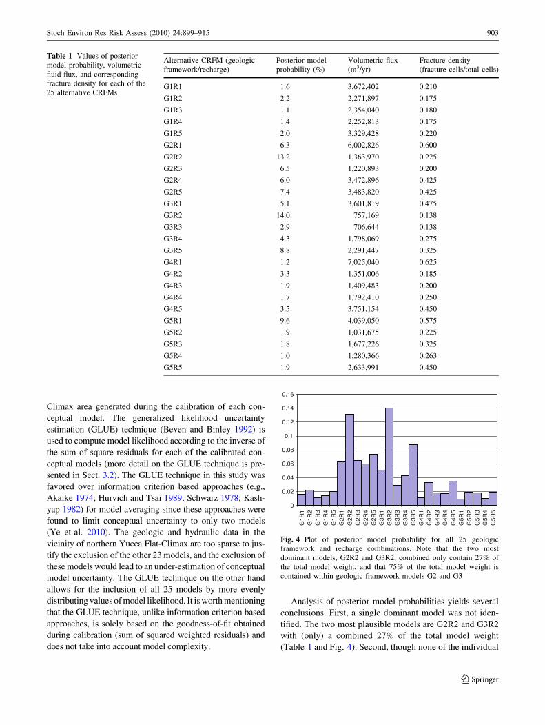
Analysis of posterior model probabilities yields several

conclusions. First, a single dominant model was not iden-

tified. The two most plausible models are G2R2 and G3R2

with (only) a combined 27% of the total model weight

(Table 1 and Fig. 4). Second, though none of the individual

Table 1 Values of posterior

model probability, volumetric

fluid flux, and corresponding

fracture density for each of the

25 alternative CRFMs

Alternative CRFM (geologic

framework/recharge)

Posterior model

probability (%)

Volumetric flux

(m3/yr)

Fracture density

(fracture cells/total cells)

G1R1 1.6 3,672,402 0.210

G1R2 2.2 2,271,897 0.175

G1R3 1.1 2,354,040 0.180

G1R4 1.4 2,252,813 0.175

G1R5 2.0 3,329,428 0.220

G2R1 6.3 6,002,826 0.600

G2R2 13.2 1,363,970 0.225

G2R3 6.5 1,220,893 0.200

G2R4 6.0 3,472,896 0.425

G2R5 7.4 3,483,820 0.425

G3R1 5.1 3,601,819 0.475

G3R2 14.0 757,169 0.138

G3R3 2.9 706,644 0.138

G3R4 4.3 1,798,069 0.275

G3R5 8.8 2,291,447 0.325

G4R1 1.2 7,025,040 0.625

G4R2 3.3 1,351,006 0.185

G4R3 1.9 1,409,483 0.200

G4R4 1.7 1,792,410 0.250

G4R5 3.5 3,751,154 0.450

G5R1 9.6 4,039,050 0.575

G5R2 1.9 1,031,675 0.225

G5R3 1.8 1,677,226 0.325

G5R4 1.0 1,280,366 0.263

G5R5 1.9 2,633,991 0.450

0

0.02

0.04

0.06

0.08

0.1

0.12

0.14

0.16

G1R

1G

1R2

G1R

3G

1R4

G1R

5G

2R1

G2R

2G

2R3

G2R

4G

2R5

G3R

1G

3R2

G3R

3G

3R4

G3R

5G

4R1

G4R

2G

4R3

G4R

4G

4R5

G5R

1G

5R2

G5R

3G

5R4

G5R

5

Fig. 4 Plot of posterior model probability for all 25 geologic

framework and recharge combinations. Note that the two most

dominant models, G2R2 and G3R2, combined only contain 27% of

the total model weight, and that 75% of the total model weight is

contained within geologic framework models G2 and G3


123

models are dominant, the geologic framework models,

specifically G2 and G3 that combined account for nearly

75% of the total model weight, have more influence on

posterior model probabilities than recharge models. This

should not be surprising because posterior probability is

heavily influenced by model likelihood values determined

during model calibration, and the geologic framework

exerts more control on flow than recharge (i.e., recharge

variations can be accommodated to some extent by the

range in hydraulic conductivity values assigned to different

hydrostratigraphic units). The broad distribution of pos-

terior probability across all alternative conceptual models

influence radionuclide flux estimates, yet these flux esti-

mates will clearly be most heavily influenced by geologic

framework models G2 and G3.

3 Simulation of flow and radionuclide transport

in the Climax stock

The Climax stock is a fractured intrusive body consisting

of low-permeability Cretaceous-age monzogranite and

granodiorite. The stock is nearly circular at depth, covering

an area of approximately 200 km2 and extending to a depth

of 7.5 km. The three underground nuclear tests at Climax

were conducted near or just below the water table. To

maintain consistency with the Underground Test Area

protocol, the tests and their radionuclide source term were

projected to the saturated zone due to their close proximity

to the water table and to avoid the complexity of radio-

nuclide migration in the vadose zone. This is a conserva-

tive measure with respect to the downstream migration of

radionuclides.

Local-scale modeling efforts consider the saturated

portion of the Climax stock exclusively and are based on

the discrete fracture network (DFN) conceptual model

where rock fractures embedded within a low permeability

matrix provide primary pathways for fluid flow and

radionuclide migration. Thus, according to this conceptual

model, potential radionuclide migration from the Hard Hat,

Pile Driver and Tiny Tot underground tests is controlled by

physical and hydraulic properties of interconnected frac-

ture networks. This conceptual model is supported by the

degree of fracturing observed at the Climax stock and the

large contrasts between field-scale hydraulic conductivity

estimates (10-7 to 10-10 m/s) and laboratory hydraulic

conductivity estimates of unfractured rock cores (10-12 to

10-15 m/s) (Murray 1980, 1981).

3.1 Fracture continuum model

The scale of the Climax stock (several kilometers) as

compared to the scale of individual fractures exceeds the

computational capacity of three-dimensional DFN models.

Instead, a fracture zone continuum approach, which

establishes a hierarchy between model cells by assigning

properties of either discrete fracture zones or an upscaled

rock matrix, is used to simulate steady-state, three-dimen-

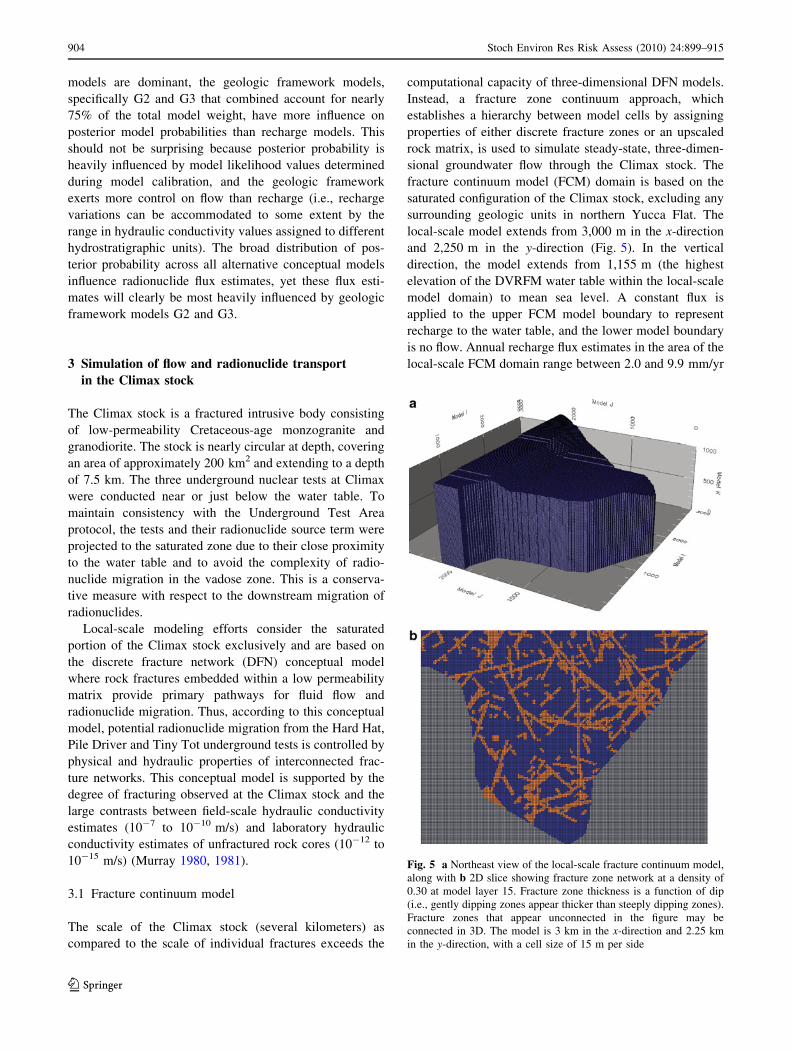
sional groundwater flow through the Climax stock. The

fracture continuum model (FCM) domain is based on the

saturated configuration of the Climax stock, excluding any

surrounding geologic units in northern Yucca Flat. The

local-scale model extends from 3,000 m in the x-direction

and 2,250 m in the y-direction (Fig. 5). In the vertical

direction, the model extends from 1,155 m (the highest

elevation of the DVRFM water table within the local-scale

model domain) to mean sea level. A constant flux is

applied to the upper FCM model boundary to represent

recharge to the water table, and the lower model boundary

is no flow. Annual recharge flux estimates in the area of the

local-scale FCM domain range between 2.0 and 9.9 mm/yr

Fig. 5 a Northeast view of the local-scale fracture continuum model,

along with b 2D slice showing fracture zone network at a density of

0.30 at model layer 15. Fracture zone thickness is a function of dip

(i.e., gently dipping zones appear thicker than steeply dipping zones).

Fracture zones that appear unconnected in the figure may be

connected in 3D. The model is 3 km in the x-direction and 2.25 km

in the y-direction, with a cell size of 15 m per side


123

(Table 2). The lack of an alluvial mask in the area of the

CRFM containing the local-scale FCM model domain

yields identical recharge estimates of 4.8 mm/yr for both

chloride mass-balance models. In general, recharge applied

to the local-scale FCM accounts for only 1% of the total

volumetric flux through the granite rock mass. All lateral

FCM boundaries are constant head using values interpo-

lated from each CRFM. A finite-difference groundwater

flow code, MODFLOW-2000 (Harbaugh et al. 2000),

solves the steady-state groundwater flow equation for both

fracture networks and rock matrix. A subset of 200 fracture

network zone realizations is generated for each of the 25

CRFM using standard Monte Carlo techniques to ade-

quately sample fracture network parameters while staying

within computational constraints.

Fracture zone networks are randomly generated for

seven fracture sets according to a compound Poisson pro-

cess for fracture location, a Fisher distribution for vari-

ability about mean fracture set orientations, a truncated

Pareto distribution for fracture length, a lognormal distri-

bution for fracture hydraulic conductivity, and an algo-

rithm, based on the ratio between fracture-occupied cells

and total cells in the model domain, to control fracture

density (Appendix). These random fracture zone networks

are then mapped onto a continuum grid with a constant cell

size of 15 m 9 15 m 9 15 m (Fig. 5). A novel mapping

algorithm, based on the equation of a plane, is used to

accurately map discrete fractures (as fracture zones) of any

strike and dip orientation as two-dimensional planar fea-

tures within a three-dimensional finite-difference model

domain. The use of a finite-difference grid to simulate

discharge in a fracture that is not aligned with the grid

requires an adjustment for longer flow paths (Botros et al.

2008; Reeves et al. 2008a):

KMODFLOW ¼ Kfracture � ½sin jhj þ cos jhj� ð2Þ

where the correction factor sin |h| ? cos |h| ensures a

correct amount of flux through grid mapped fractures ori-

ented at angle h to the grid. Fractures mapped onto the grid

are randomly assigned values of hydraulic conductivity

according to one of the two lognormal distributions

described in the Appendix. Cells unoccupied by fractures

represent an upscaled matrix with a small degree of

background fracturing and are assigned a hydraulic con-

ductivity value of 10-10 m/s. Interestingly, this upscaled

matrix hydraulic conductivity value is very close to the

mean hydraulic conductivity value used in the stochastic

continuum model of Hendricks Franssen and Gomez-

Hernandez (2002) to represent an upscaled granite rock

matrix with background fracturing.

3.2 Flow model calibration and weighting

There are no reliable head measurements in the Climax

stock; therefore, head values could not be used as cali-

bration targets. Instead, each of the 25 CRFMs was used to

provide both boundary conditions and target volumetric

flux values for each 200 realization subset of the 5,000 total

FCM flow realizations. The target volumetric flux is

defined as total annual flow [m3/yr] simulated through cells

of the CRFM grid that correspond to the local-scale FCM

domain. Calibration of the fracture continuum realizations

to all CRFMs was further complicated by the approximate

order-of-magnitude difference in the 25 CRFM volumetric

flux values (706,644 to 7,025,040 m3/yr) (Table 1).

The calibration of fracture network parameters to the

large range in volumetric flux values for the 25 conceptual

models could possibly occur by either adjusting mean

hydraulic conductivity or fracture density. Of these two

parameters, fracture density was deemed more uncertain as

the frequency of flowing fractures, defined as the inter-

connected network of fractures responsible for flow, is

completely unknown. While fracture hydraulic conductiv-

ity is also uncertain, Murray (1980, 1981) suggested a

range of fracture hydraulic conductivity values between

10-7 to 10-10 m/s based on bulk hydraulic conductivity

values obtained from hydraulic tests in the Climax stock.

The calibration of volumetric flux to fracture density

implies that each CRFM, through its flux value, represents

a different level of network connectivity as flow is

Table 2 Values of recharge

flux for each alternative

conceptual model in the local-

scale fracture continuum model

Recharge model Recharge rate (mm/yr) Recharge rate (m3/yr)

Modified Maxey-Eakin 6.8 24,655

Net infiltration I 9.9 36,262

Net infiltration II 2.0 7,173

Chloride mass-balance I 4.8 17,679

Chloride mass-balance II 4.8 17,679

Table 3 Statistics of fracture sets in the SFT-C database

Set1 Set2 Set3 Set4 Set5 Set6 Set7

Prior probability 0.03 0.13 0.10 0.14 0.13 0.32 0.15

Mean strike 125 317 360 321 289 48 N/A

Mean dip 19 25 85 83 82 80 N/A

Dispersion (j) 65 37 33 24 23 18 N/A


123

proportional to fracture connectivity (assuming the distri-

bution hydraulic conductivity is held equal), and increases

in fracture density in the fracture zone generation code lead

to greater levels of network connectivity.

Calibration of volumetric flux to fracture density using

least-square methods to minimize volumetric flux residuals

(e.g., Doherty 2000) proved unsuccessful due to objective

functions with several local minima, and the finding that

volumetric flux values through individual network real-

izations having the same density can vary over several

orders of magnitude. The variability in flux values for

randomly generated networks with identical density values

is attributed to the degree of network connectivity and the

hydraulic conductivity values assigned to individual frac-

ture segments. As an alternative to inverse methods, FCM

calibration was considered to be achieved when the geo-

metric mean of simulated flow for all 200 realizations is

within ± 5% of the CRFM target flux. Mean fracture set

hydraulic conductivity values of 10-7 and 10-8 m/s were

found to simulate the range in CRFM volumetric flux by

producing backbones above the percolation threshold at

lower volumetric flux values (necessary for network flow),

yet only occupy approximately half of the model grid

at higher volumetric flux values (necessary for the

implementation of the fracture continuum method). A trial-

and-error process was used to determine values of fracture

density.

In a standard Monte Carlo simulation, all of these real-

izations, regardless of flux values, would have equal weight.

However, given the extreme variability in flux across all

realizations, it is reasonable to assume that flow realizations

that more closely match the target flux value for a CRFM

should receive more weight than flow realizations that show

a poor match to the given target flux. Since the calibration of

flux was not achieved from a least-square or maximum

likelihood perspective, Bayesian model averaging tech-

niques (e.g., Neuman 2003; Vrugt et al. 2008) were not used.

Instead, a generalized likelihood uncertainty estimate

(GLUE) technique (Beven and Binley 1992) is used to assign

weights to each of the 200 individual flow realization subsets

for a given CRFM according to:

L Fjhijð Þ ¼ 1

Ei

� �N

ð3Þ

where L Fjhijð Þ is the likelihood of the vector of simulated

flux values for the local-scale FC realizations, F; given the

parameter set, h: Ei is an objective function and N is a

likelihood shape factor that can range from zero to infinity.

By assuming a weak correlation between flux in each

CRFM and the corresponding FCM realizations, the

objective function can be defined as: Ei ¼ ðFluxi �FluxtÞ2; where Fluxi are flux values for FCM realizations

with index i, and Fluxt is the target flux value for the

corresponding CRFM. The selection of N is central to the

GLUE weighting method. A value of zero describes a

standard Monte Carlo realization where all realizations

have equal weight. As N increases from zero toward

infinity, probability is shifted towards the realizations that

best match the objective function. Traditionally a value of

1 is used for N, but the shape factor can also be chosen by

the user (Beven and Binley 1992).

Flux values in the fracture zone networks are con-

strained only by the range and distribution of the network

parameters and the constant head boundary conditions

from the corresponding CRFM. As a consequence, the

degree of variability in values of flux for these networks is

much greater than would be expected if regional flow

constraints were placed on the local-scale FCM. To address

variability in volumetric flux through the Climax stock

while adhering to regional flow constraints, 200 regional-

scale flow realizations were generated for each CRFM. The

distribution of flux values from the regional-scale realiza-

tions, where parametric uncertainty is addressed by using a

covariance matrix for each of the 25 calibrated regional

models (i.e., for a given parameter, its calibrated value is

the mean and the deviation about the mean is described by

its covariance), are thought to better reflect the variability

in flow that is possible for the Climax stock. These regio-

nal-scale CRFM flux values are used in conjunction with

flux values from the local-scale FCM to define N.

Values of flux from the regional-scale realizations are

sorted and ranked to compute an empirical cumulative

distribution function (CDF). Next, given an arbitrary value

of N, an empirical CDF for the local-scale FCM flow

weights, L Fjhijð Þ is computed according to (3). Flux values

corresponding to the 95% confidence intervals, 0.025 and

0.975, are compared for both the regional-scale and local-

scale models. The value of N, which controls the distri-

bution of weights for the local-scale model, is then changed

until the difference in flux values corresponding to the

lower and upper 95% confidence intervals is minimized

(Franks et al. 1999; Beven and Freer 2001). By following

this procedure for all 25 CRFMs, N was found to range

between 0.44 and 1.0. The mean (and median) of the dis-

tribution of N is 0.69. The use of this value shifts proba-

bility weight to realizations that best match the target flux

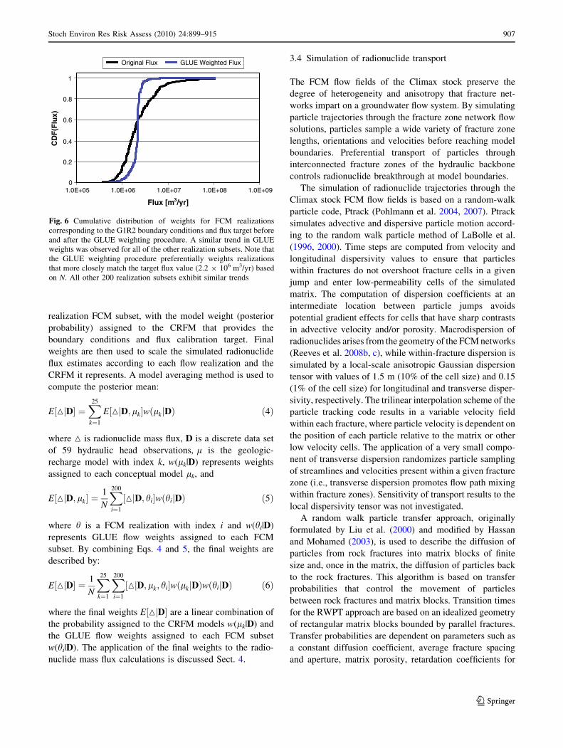
value. Figure 6 shows the influence of the cumulative

distribution of model weights based on flux for one of the

200 realization subsets.

3.3 Model averaging

Final weights for each FCM flow realization are a combi-

nation of the GLUE flow weights assigned to the 200-


123

realization FCM subset, with the model weight (posterior

probability) assigned to the CRFM that provides the

boundary conditions and flux calibration target. Final

weights are then used to scale the simulated radionuclide

flux estimates according to each flow realization and the

CRFM it represents. A model averaging method is used to

compute the posterior mean:

E½MjD� ¼X25

k¼1

E½MjD; lk�wðlkjDÞ ð4Þ

where M is radionuclide mass flux, D is a discrete data set

of 59 hydraulic head observations, l is the geologic-

recharge model with index k, w(lk|D) represents weights

assigned to each conceptual model lk, and

E½MjD; lk� ¼1

N

X200

i¼1

½MjD; hi�wðhijDÞ ð5Þ

where h is a FCM realization with index i and w(hi|D)

represents GLUE flow weights assigned to each FCM

subset. By combining Eqs. 4 and 5, the final weights are

described by:

E½MjD� ¼ 1

N

X25

k¼1

X200

i¼1

½MjD; lk; hi�wðlkjDÞwðhijDÞ ð6Þ

where the final weights E½MjD� are a linear combination of

the probability assigned to the CRFM models w(lk|D) and

the GLUE flow weights assigned to each FCM subset

w(hi|D). The application of the final weights to the radio-

nuclide mass flux calculations is discussed Sect. 4.

3.4 Simulation of radionuclide transport

The FCM flow fields of the Climax stock preserve the

degree of heterogeneity and anisotropy that fracture net-

works impart on a groundwater flow system. By simulating

particle trajectories through the fracture zone network flow

solutions, particles sample a wide variety of fracture zone

lengths, orientations and velocities before reaching model

boundaries. Preferential transport of particles through

interconnected fracture zones of the hydraulic backbone

controls radionuclide breakthrough at model boundaries.

The simulation of radionuclide trajectories through the

Climax stock FCM flow fields is based on a random-walk

particle code, Ptrack (Pohlmann et al. 2004, 2007). Ptrack

simulates advective and dispersive particle motion accord-

ing to the random walk particle method of LaBolle et al.

(1996, 2000). Time steps are computed from velocity and

longitudinal dispersivity values to ensure that particles

within fractures do not overshoot fracture cells in a given

jump and enter low-permeability cells of the simulated

matrix. The computation of dispersion coefficients at an

intermediate location between particle jumps avoids

potential gradient effects for cells that have sharp contrasts

in advective velocity and/or porosity. Macrodispersion of

radionuclides arises from the geometry of the FCM networks

(Reeves et al. 2008b, c), while within-fracture dispersion is

simulated by a local-scale anisotropic Gaussian dispersion

tensor with values of 1.5 m (10% of the cell size) and 0.15

(1% of the cell size) for longitudinal and transverse disper-

sivity, respectively. The trilinear interpolation scheme of the

particle tracking code results in a variable velocity field

within each fracture, where particle velocity is dependent on

the position of each particle relative to the matrix or other

low velocity cells. The application of a very small compo-

nent of transverse dispersion randomizes particle sampling

of streamlines and velocities present within a given fracture

zone (i.e., transverse dispersion promotes flow path mixing

within fracture zones). Sensitivity of transport results to the

local dispersivity tensor was not investigated.

A random walk particle transfer approach, originally

formulated by Liu et al. (2000) and modified by Hassan

and Mohamed (2003), is used to describe the diffusion of

particles from rock fractures into matrix blocks of finite

size and, once in the matrix, the diffusion of particles back

to the rock fractures. This algorithm is based on transfer

probabilities that control the movement of particles

between rock fractures and matrix blocks. Transition times

for the RWPT approach are based on an idealized geometry

of rectangular matrix blocks bounded by parallel fractures.

Transfer probabilities are dependent on parameters such as

a constant diffusion coefficient, average fracture spacing

and aperture, matrix porosity, retardation coefficients for

0

0.2

0.4

0.6

0.8

1

1.0E+05 1.0E+06 1.0E+07 1.0E+08 1.0E+09

Flux [m3/yr]

CD

F(F

lux)

Original Flux GLUE Weighted Flux

Fig. 6 Cumulative distribution of weights for FCM realizations

corresponding to the G1R2 boundary conditions and flux target before

and after the GLUE weighting procedure. A similar trend in GLUE

weights was observed for all of the other realization subsets. Note that

the GLUE weighting procedure preferentially weights realizations

that more closely match the target flux value (2.2 9 106 m3/yr) based

on N. All other 200 realization subsets exhibit similar trends


123

the matrix and fractures, and advection in the matrix and

fractures (refer to Hassan and Mohamed (2003) for more

detail). An average fracture spacing of 6 m, based on the

assumption that only 10% of the total fracture population

contributes to flow (Dershowitz et al. 2000), is used to

parameterize the random walk particle transfer algorithm.

A constant aperture value corresponding to the geometric

mean aperture from the SFT-C database and a constant

diffusion coefficient of 1.0 9 10-6 m2/d, representative of

a generic radionuclide, is used for all transport simulations.

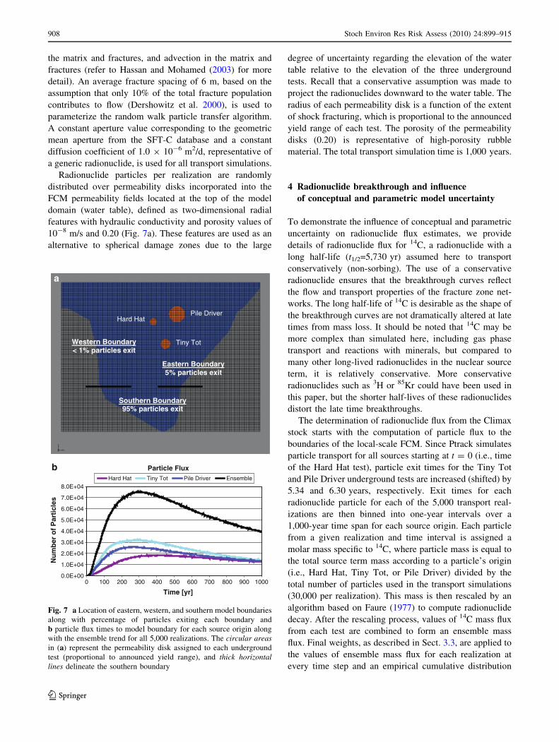
Radionuclide particles per realization are randomly

distributed over permeability disks incorporated into the

FCM permeability fields located at the top of the model

domain (water table), defined as two-dimensional radial

features with hydraulic conductivity and porosity values of

10-8 m/s and 0.20 (Fig. 7a). These features are used as an

alternative to spherical damage zones due to the large

degree of uncertainty regarding the elevation of the water

table relative to the elevation of the three underground

tests. Recall that a conservative assumption was made to

project the radionuclides downward to the water table. The

radius of each permeability disk is a function of the extent

of shock fracturing, which is proportional to the announced

yield range of each test. The porosity of the permeability

disks (0.20) is representative of high-porosity rubble

material. The total transport simulation time is 1,000 years.

4 Radionuclide breakthrough and influence

of conceptual and parametric model uncertainty

To demonstrate the influence of conceptual and parametric

uncertainty on radionuclide flux estimates, we provide

details of radionuclide flux for 14C, a radionuclide with a

long half-life (t1/2=5,730 yr) assumed here to transport

conservatively (non-sorbing). The use of a conservative

radionuclide ensures that the breakthrough curves reflect

the flow and transport properties of the fracture zone net-

works. The long half-life of 14C is desirable as the shape of

the breakthrough curves are not dramatically altered at late

times from mass loss. It should be noted that 14C may be

more complex than simulated here, including gas phase

transport and reactions with minerals, but compared to

many other long-lived radionuclides in the nuclear source

term, it is relatively conservative. More conservative

radionuclides such as 3H or 85Kr could have been used in

this paper, but the shorter half-lives of these radionuclides

distort the late time breakthroughs.

The determination of radionuclide flux from the Climax

stock starts with the computation of particle flux to the

boundaries of the local-scale FCM. Since Ptrack simulates

particle transport for all sources starting at t = 0 (i.e., time

of the Hard Hat test), particle exit times for the Tiny Tot

and Pile Driver underground tests are increased (shifted) by

5.34 and 6.30 years, respectively. Exit times for each

radionuclide particle for each of the 5,000 transport real-

izations are then binned into one-year intervals over a

1,000-year time span for each source origin. Each particle

from a given realization and time interval is assigned a

molar mass specific to 14C, where particle mass is equal to

the total source term mass according to a particle’s origin

(i.e., Hard Hat, Tiny Tot, or Pile Driver) divided by the

total number of particles used in the transport simulations

(30,000 per realization). This mass is then rescaled by an

algorithm based on Faure (1977) to compute radionuclide

decay. After the rescaling process, values of 14C mass flux

from each test are combined to form an ensemble mass

flux. Final weights, as described in Sect. 3.3, are applied to

the values of ensemble mass flux for each realization at

every time step and an empirical cumulative distribution

Pile Driver Hard Hat

Tiny Tot

Southern Boundary 95% particles exit

Eastern Boundary 5% particles exit

Western Boundary < 1% particles exit

Particle Flux

0.0E+00

1.0E+04

2.0E+04

3.0E+04

4.0E+04

5.0E+04

6.0E+04

7.0E+04

8.0E+04

0 100 200 300 400 500 600 700 800 900 1000

Time [yr]

Nu

mb

er o

f P

arti

cles

Hard Hat Tiny Tot Pile Driver Ensemble

a

b

Fig. 7 a Location of eastern, western, and southern model boundaries

along with percentage of particles exiting each boundary and

b particle flux times to model boundary for each source origin along

with the ensemble trend for all 5,000 realizations. The circular areasin (a) represent the permeability disk assigned to each underground

test (proportional to announced yield range), and thick horizontallines delineate the southern boundary


123

function (CDF) is computed from the final weights. Values

of ensemble mass flux corresponding to the median and the

upper and lower 95% confidence intervals (U95 and L95)

are then determined from the empirical CDF for each time

step. Mean mass flux for a given time interval is the

product sum of mass flux values and their corresponding

weights for all 5,000 FCM realizations.

Particle breakthroughs at model boundaries (the margins

of the Climax stock) for all 5,000 transport simulations are

presented in Fig. 7. Approximately one-third of the 14C

particles exit the model domain within the total transport

time of 1,000 years. Of the particles that leave the model

domain, 26% originate from the Hard Hat test, 41% orig-

inate from the Tiny Tot test, and 33% originate from the

Pile Driver test (Fig. 7b). Differences in particle break-

through are attributed to test location relative to the

southern boundary (transport distance) and size of the

permeability disks (larger permeability disks have a greater

chance of intersection by the hydraulic backbone).

Approximately 95% of all particles exit through the

southern model boundary (Fig. 7a). This demonstrates that

the general flow direction of northeast to southwest flow

through the Climax stock (Murray 1981) is preserved in the

local-scale FCM despite the randomness of the fracture

zone networks. Particle flux at the local-scale FCM

boundaries for the Hard Hat, Tiny Tot, and Pile Driver tests

peaks at 414, 276, and 263 years, respectively (this is

without consideration of radioactive decay) (Fig. 7b). The

peak arrival time for the ensemble of the three tests occurs

at 307 years.

The raw (i.e., unprocessed) particle flux times to model

domain boundaries (Fig. 7b) incorporate conceptual model

uncertainty propagated to local-scale FCM realizations

through constant head boundary conditions, a fluid flux

calibration target, and model weights that describe the

plausibility of each model. Parametric uncertainty in the

local-scale flow model is addressed by fracture zone net-

works with random zone placement, orientation, length and

hydraulic conductivity. Further parametric uncertainty is

introduced during the simulation of transport including an

anisotropic within-fracture dispersion tensor, fracture zone

porosity (correlated with fracture K), and the random walk

particle transfer approach used to simulate the motion of

radionuclide particles between fractures and the rock

matrix. Despite the inclusion of parametric uncertainty,

fracture density—obtained through calibration to the vol-

umetric flux target for each CRFM—is the only parameter

that differs between all 200 FCM realization subsets for

each of the 25 conceptual models. All other statistical

properties of the FCM are held equal.

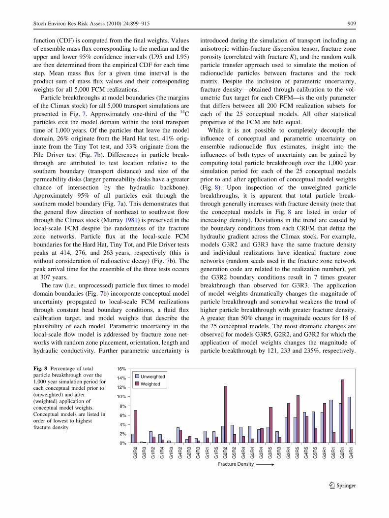
While it is not possible to completely decouple the

influence of conceptual and parametric uncertainty on

ensemble radionuclide flux estimates, insight into the

influences of both types of uncertainty can be gained by

computing total particle breakthrough over the 1,000 year

simulation period for each of the 25 conceptual models

prior to and after application of conceptual model weights

(Fig. 8). Upon inspection of the unweighted particle

breakthroughs, it is apparent that total particle break-

through generally increases with fracture density (note that

the conceptual models in Fig. 8 are listed in order of

increasing density). Deviations in the trend are caused by

the boundary conditions from each CRFM that define the

hydraulic gradient across the Climax stock. For example,

models G3R2 and G3R3 have the same fracture density

and individual realizations have identical fracture zone

networks (random seeds used in the fracture zone network

generation code are related to the realization number), yet

the G3R2 boundary conditions result in 7 times greater

breakthrough than observed for G3R3. The application

of model weights dramatically changes the magnitude of

particle breakthrough and somewhat weakens the trend of

higher particle breakthrough with greater fracture density.

A greater than 50% change in magnitude occurs for 18 of

the 25 conceptual models. The most dramatic changes are

observed for models G3R5, G2R2, and G3R2 for which the

application of model weights changes the magnitude of

particle breakthrough by 121, 233 and 235%, respectively.

0%

2%

4%

6%

8%

10%

12%

14%

16%

G3R

2

G3R

3

G1R

2

G1R

4

G1R

3

G4R

2

G2R

3

G4R

3

G1R

1

G1R

5

G2R

2

G5R

2

G4R

4

G5R

4

G3R

4

G3R

5

G5R

3

G2R

4

G2R

5

G4R

5

G5R

5

G3R

1

G5R

1

G2R

1

G4R

1

Unweighted

Weighted

Fracture Density

Fig. 8 Percentage of total

particle breakthrough over the

1,000 year simulation period for

each conceptual model prior to

(unweighted) and after

(weighted) application of

conceptual model weights.

Conceptual models are listed in

order of lowest to highest

fracture density


123

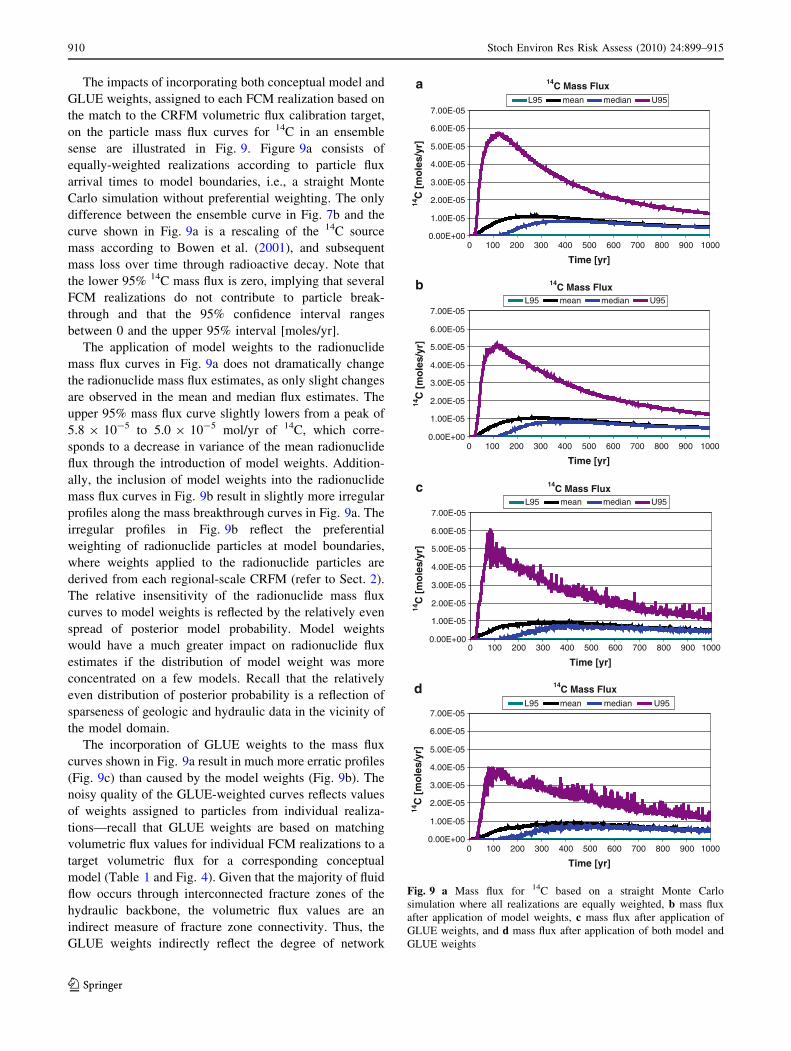
The impacts of incorporating both conceptual model and

GLUE weights, assigned to each FCM realization based on

the match to the CRFM volumetric flux calibration target,

on the particle mass flux curves for 14C in an ensemble

sense are illustrated in Fig. 9. Figure 9a consists of

equally-weighted realizations according to particle flux

arrival times to model boundaries, i.e., a straight Monte

Carlo simulation without preferential weighting. The only

difference between the ensemble curve in Fig. 7b and the

curve shown in Fig. 9a is a rescaling of the 14C source

mass according to Bowen et al. (2001), and subsequent

mass loss over time through radioactive decay. Note that

the lower 95% 14C mass flux is zero, implying that several

FCM realizations do not contribute to particle break-

through and that the 95% confidence interval ranges

between 0 and the upper 95% interval [moles/yr].

The application of model weights to the radionuclide

mass flux curves in Fig. 9a does not dramatically change

the radionuclide mass flux estimates, as only slight changes

are observed in the mean and median flux estimates. The

upper 95% mass flux curve slightly lowers from a peak of

5.8 9 10-5 to 5.0 9 10-5 mol/yr of 14C, which corre-

sponds to a decrease in variance of the mean radionuclide

flux through the introduction of model weights. Addition-

ally, the inclusion of model weights into the radionuclide

mass flux curves in Fig. 9b result in slightly more irregular

profiles along the mass breakthrough curves in Fig. 9a. The

irregular profiles in Fig. 9b reflect the preferential

weighting of radionuclide particles at model boundaries,

where weights applied to the radionuclide particles are

derived from each regional-scale CRFM (refer to Sect. 2).

The relative insensitivity of the radionuclide mass flux

curves to model weights is reflected by the relatively even

spread of posterior model probability. Model weights

would have a much greater impact on radionuclide flux

estimates if the distribution of model weight was more

concentrated on a few models. Recall that the relatively

even distribution of posterior probability is a reflection of

sparseness of geologic and hydraulic data in the vicinity of

the model domain.

The incorporation of GLUE weights to the mass flux

curves shown in Fig. 9a result in much more erratic profiles

(Fig. 9c) than caused by the model weights (Fig. 9b). The

noisy quality of the GLUE-weighted curves reflects values

of weights assigned to particles from individual realiza-

tions—recall that GLUE weights are based on matching

volumetric flux values for individual FCM realizations to a

target volumetric flux for a corresponding conceptual

model (Table 1 and Fig. 4). Given that the majority of fluid

flow occurs through interconnected fracture zones of the

hydraulic backbone, the volumetric flux values are an

indirect measure of fracture zone connectivity. Thus, the

GLUE weights indirectly reflect the degree of network

14C Mass Flux

0.00E+00

1.00E-05

2.00E-05

3.00E-05

4.00E-05

5.00E-05

6.00E-05

7.00E-05

0 100 200 300 400 500 600 700 800 900 1000

0 100 200 300 400 500 600 700 800 900 1000

0 100 200 300 400 500 600 700 800 900 1000

0 100 200 300 400 500 600 700 800 900 1000

Time [yr]

14C

[m

ole

s/yr

]

L95 mean median U95

14C Mass Flux

0.00E+00

1.00E-05

2.00E-05

3.00E-05

4.00E-05

5.00E-05

6.00E-05

7.00E-05

Time [yr]

14C

[m

ole

s/yr

]

L95 mean median U95

14C Mass Flux

0.00E+00

1.00E-05

2.00E-05

3.00E-05

4.00E-05

5.00E-05

6.00E-05

7.00E-05

Time [yr]

14C

[m

ole

s/yr

]

L95 mean median U95

14C Mass Flux

0.00E+00

1.00E-05

2.00E-05

3.00E-05

4.00E-05

5.00E-05

6.00E-05

7.00E-05

Time [yr]

14C

[m

ole

s/yr

]

L95 mean median U95

a

c

d

b

Fig. 9 a Mass flux for 14C based on a straight Monte Carlo

simulation where all realizations are equally weighted, b mass flux

after application of model weights, c mass flux after application of

GLUE weights, and d mass flux after application of both model and

GLUE weights


123

connectivity which represents parametric uncertainty pro-

duced by random fracture zone placement, orientation,

length and hydraulic conductivity. Despite the noise, the

GLUE weighted mass flux curves (Fig. 9c) follow the same

general trend as the equally weighted Monte Carlo mass

flux curves (Fig. 9a).

The final weights assigned to the mass flux curves are a

combination of both model and GLUE weights (refer to

Sect. 3.3). The multiplication of these weights increases the

amplitude of the noise as the final radionuclide mass flux

curves exhibit the most erratic profiles (Fig. 9d). The mag-

nitude of the mass flux curves subject to the final weights

shows a more dramatic decrease in peak magnitude for all

confidence intervals, except for the lower 95% confidence

interval which equals zero for all cases. The upper 95%

confidence interval decreases from approximately 5.8 9

10-5 mol/yr of 14C for the equally weighted curves in

Fig. 9a to 3. 8 9 10-5 mol/yr. The combined model weights

appear to exert the most influence on the magnitude of early

breakthroughs. The greatest decrease in the estimates of

mass flux, particulary the variance, is to be expected after the

application of the final weights since these weights prefer-

entially weight particle breakthroughs from conceptual

models that are most plausible and FCM realizations that

best match the volumetric flux calibration target.

5 Conclusions

Detailed numerical flow and transport simulations are used

to support CAU modeling efforts by predicting the flux of

radionuclides from three underground nuclear tests con-

ducted in a fractured granite rock mass on the Nevada Test

Site. A regional-scale model incorporates conceptual

model uncertainty through the inclusion of five models of

hydrostratigraphy and five models describing recharge

prcoesses for a total of 25 hydrostratigraphic–recharge

combinations. Uncertainty from each of the 25 models is

propagated to the local-scale model through boundary

conditions, a fluid flux calibration target, and model

weights that describe the plausibility of each conceptual

model. Radionuclide transport estimates for the Climax

stock are based on a local-scale fracture continuum model

parameterized according to analysis of site-specific rock

fracture data, and calibration of fracture density to volu-

metric flux. Each local-scale FCM is assigned a GLUE

weight according to the match between flux of the reali-

zation and the target volumetric flux.

The flux calibration target was found to correlate with

fracture density, and particle breakthroughs were generally

found to increase with increases in fracture density.

Boundary conditions extrapolated from the conceptual

models exerted a secondary influence on radionuclide

breakthrough for models with equal fracture density. The

incorporation of model and GLUE weights results in both

noise about the original (unweighted) mass flux curves and

decreases in the variance and expected value of radionuclide

mass flux. The moderate insensitivity of the radionuclide

flux estimates to the final weights is based on the more or less

even distribution of posterior model probability assigned to

each of the conceptual models due to sparse geologic and

hydraulic data. It is anticipated the concentration of model

weight around only two models would dramatically affect

the radionuclide mass flux estimates after weighting of

particle breakthroughs produced by each model.

Acknowledgements This research was supported by the U.S.

Department of Energy, National Nuclear Security Administration

Nevada Site Office under Contract DE-AC52-00NV13609 with the

Desert Research Institute. Special thanks goes to the guest editor Dr.

Yu-Feng Lin and Drs. Yonas Demissi, Abhishek Singh and Andrew

F.B. Tompson for constructive comments that greatly improved the

quality of the manuscript.

Appendix: Fracture characterization

Numerical modeling of fluid flow in fracture dominated

subsurface flow regimes requires statistical analysis of

fracture data for the determination of fracture properties,

such as fracture sets and their mean orientation, length,

spacing and distribution, density, and permeability of

individual fractures or zones (e.g., Munier 2004; Reeves

et al. 2008a). Fracture characterization at the Climax stock

is based on the Spent Fuel Test—Climax (SFT-C) Geologic

Structure Database (Yow 1984) that consists of data

describing joints, faults and shear zones (sample population

n = 2, 591) that were collected during fracture mapping

efforts in tunnel drifts constructed for the Climax Spent

Fuel Test.

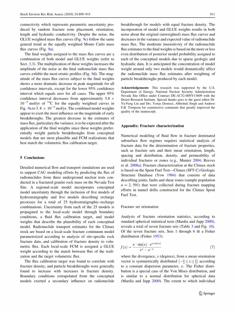
Fracture set orientation

Analysis of fracture orientation statistics, according to

standard spherical statistical tests (Mardia and Jupp 2000),

reveals a total of seven fracture sets (Table 3 and Fig. 10).

Of the seven fracture sets, Sets 1 through 6 fit a Fisher

distribution (Fisher 1953):

f ðxÞ ¼ j � sinðxÞ � ej�cosðxÞ

ej � e�jð7Þ

where the divergence, x (degrees), from a mean orientation

vector is symmetrically distributed ð�p2� x� p

2Þ according

to a constant dispersion parameter, j. The Fisher distri-

bution is a special case of the Von Mises distribution, and

is similar to a normal distribution for spherical data

(Mardia and Jupp 2000). The extent to which individual


123

fractures cluster around a mean orientation is proportional

to values of j (i.e., higher values of j describe higher

degrees of clustering). Values of j for natural rock frac-

tures range between 10 and 300 (Kemeny and Post 2003).

Stochastic simulation of Fisher random deviates is based

on a method by Wood (1994). The occurrence of each

fracture set is governed by the prior probabilities listed in

Table 3. The distribution of fracture orientation for Set 7 is

assumed uniform.

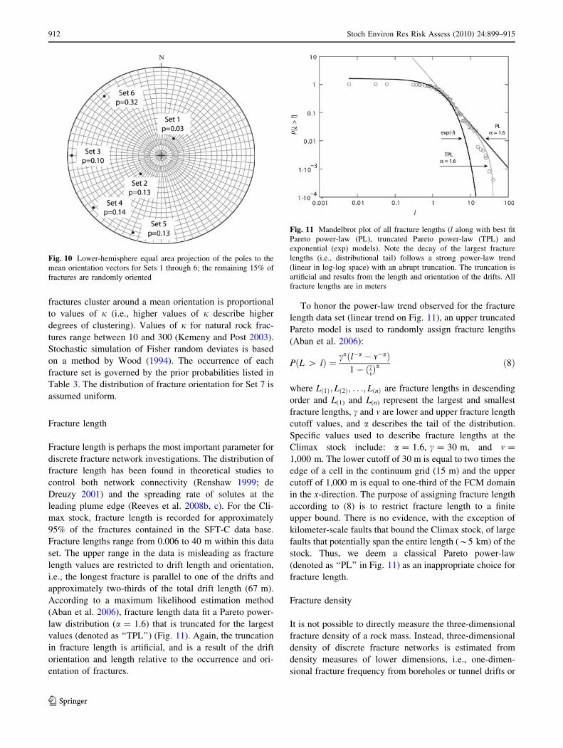
Fracture length

Fracture length is perhaps the most important parameter for

discrete fracture network investigations. The distribution of

fracture length has been found in theoretical studies to

control both network connectivity (Renshaw 1999; de

Dreuzy 2001) and the spreading rate of solutes at the

leading plume edge (Reeves et al. 2008b, c). For the Cli-

max stock, fracture length is recorded for approximately

95% of the fractures contained in the SFT-C data base.

Fracture lengths range from 0.006 to 40 m within this data

set. The upper range in the data is misleading as fracture

length values are restricted to drift length and orientation,

i.e., the longest fracture is parallel to one of the drifts and

approximately two-thirds of the total drift length (67 m).

According to a maximum likelihood estimation method

(Aban et al. 2006), fracture length data fit a Pareto power-

law distribution (a = 1.6) that is truncated for the largest

values (denoted as ‘‘TPL’’) (Fig. 11). Again, the truncation

in fracture length is artificial, and is a result of the drift

orientation and length relative to the occurrence and ori-

entation of fractures.

To honor the power-law trend observed for the fracture

length data set (linear trend on Fig. 11), an upper truncated

Pareto model is used to randomly assign fracture lengths

(Aban et al. 2006):

PðL [ lÞ ¼ caðl�a � m�aÞ1� ðcmÞ

a ð8Þ

where Lð1Þ; Lð2Þ; . . .; LðnÞ are fracture lengths in descending

order and L(1) and L(n) represent the largest and smallest

fracture lengths, c and m are lower and upper fracture length

cutoff values, and a describes the tail of the distribution.

Specific values used to describe fracture lengths at the

Climax stock include: a = 1.6, c = 30 m, and m =

1,000 m. The lower cutoff of 30 m is equal to two times the

edge of a cell in the continuum grid (15 m) and the upper

cutoff of 1,000 m is equal to one-third of the FCM domain

in the x-direction. The purpose of assigning fracture length

according to (8) is to restrict fracture length to a finite

upper bound. There is no evidence, with the exception of

kilometer-scale faults that bound the Climax stock, of large

faults that potentially span the entire length (*5 km) of the

stock. Thus, we deem a classical Pareto power-law

(denoted as ‘‘PL’’ in Fig. 11) as an inappropriate choice for

fracture length.

Fracture density

It is not possible to directly measure the three-dimensional

fracture density of a rock mass. Instead, three-dimensional

density of discrete fracture networks is estimated from

density measures of lower dimensions, i.e., one-dimen-

sional fracture frequency from boreholes or tunnel drifts or

Fig. 10 Lower-hemisphere equal area projection of the poles to the

mean orientation vectors for Sets 1 through 6; the remaining 15% of

fractures are randomly oriented

Fig. 11 Mandelbrot plot of all fracture lengths (l along with best fit

Pareto power-law (PL), truncated Pareto power-law (TPL) and

exponential (exp) models). Note the decay of the largest fracture

lengths (i.e., distributional tail) follows a strong power-law trend

(linear in log-log space) with an abrupt truncation. The truncation is

artificial and results from the length and orientation of the drifts. All

fracture lengths are in meters


123

two-dimensional density from outcrops or fracture trace

maps. Fracture frequency in the SFT-C database, based on

fracture mapping along tunnel drifts, is relatively high and

ranges between 2.0 to 5.5 fractures per meter. However, the

high fracture spacing in the SFT-C database is misleading

as the frequency of ‘‘flowing’’ or conductive fractures is

not considered.

Field observations for fractured rock masses indicate

that rock volumes are often intersected by only a few

dominant fractures and only approximately 10% (or less)

of the total fracture population contributes to flow (Der-

showitz et al. 2000). This implies that 90% of fractures in

the SFT-C database are not connected to the hydraulic

backbone. Two specific studies at Climax provide some

insight into the frequency of open fractures. In a tunnel

drift for the SFT-C experiments, a series of five boreholes

extending 9 to 12 meters below the tunnel drift yielded

permeability values typical of unfractured granite cores

(Ballou 1979). This indicates that the borehole array, which

is on the scale of a grid cell, only intersects either solid

rock or rock with ‘‘healed’’ fractures. ‘‘Healed’’ fractures

(i.e., veins) refer to fractures containing mineral precipi-

tates (e.g., calcite) and are, therefore, not open to flow.

Several instances of healed fractures were documented in

the SFT-C database by Yow (1984)—these fractures were

excluded from the frequency analysis when recorded. In

the permeability test conducted by Isherwood et al. (1982),

only 2 out of 10 (20%) fractures in a densely fractured zone

were open and had permeability values higher than the

background matrix.

Given the high level of uncertainty in fracture density,

this parameter is determined in the fracture continuum

model during calibration (Table 1). Refer to Sect. 3.2 for

additional discussion.

Hydraulic conductivity

Only a handful of field-scale hydraulic conductivity (K)

measurements exist for the Climax stock (on the order of

10-7 to 10-10 m/s) (Murray 1980, 1981). These values

describe the bulk hydraulic conductivity of the fractured

stock, and most likely underestimate variability in fracture

K since these estimates are based on hydraulic testing over

large open borehole intervals where properties of multiple

fractures are averaged. This narrow range (3 orders of

magnitude) is inconsistent with other studies of highly

characterized fractured granite rock masses where values

of fracture K encompass 5–8 orders of magnitude (Paillet

1998; Guimera and Carrera 2000; Andersson et al.

2002; Hendricks Franssen and Gomez-Hernandez 2002;

Gustafson and Fransson 2005).

Instead of relying on a handful of effective permeability

measurements to parameterize a probability distribution for

fracture K, the distribution of mechanical fracture apertures

in the SFT-C database is analyzed. Recorded aperture

values are lognormally distributed with a standard devia-

tion of 1.05 (not shown) and this value is used to describe

the variability in the fracture K distributions. This value is

identical to the standard deviation of the transmissivity

distribution used by Stigsson et al. (2001) at the Aspo Hard

Rock Laboratory. Though rock fracture hydraulic con-

ductivity is proportional to mechanical aperture, correla-

tions between mechanical and equivalent hydraulic

apertures are often unreliable (Bandis et al. 1985; Cook

et al. 1990); therefore, mean values of K are not computed

from the mechanical aperture distribution. Aperture data

are used only to gauge the suitability of a lognormal dis-

tribution for fracture K and to provide an estimate of

standard deviation.

To maintain a constant conceptual model for radio-

nuclide flux estimates (refer to Sect. 3.2 for more detail),

fracture K distributions were held constant at values of

-7 and -8 (the original values of K are in units of

meters per second prior to log transformation). Both

of these mean fracture K values are within the narrow

range defined by Murray (1981). The higher mean value

of -7 m/s is assigned to fractures that belong to fracture

set 6 (32% of the fractures) (Table 3). Fractures in this

set experience the least amount of compressive stress

normal to their fracture walls, suggesting that these

fractures are potentially more permeable than fractures

oriented at other directions to the regional stress field.

The remaining fracture sets (68% of the fractures) are

assigned K values according to the lower mean K of -8.

A log10 K standard deviation value of 1.05 is applied to

all fracture sets.

Fracture porosity

The computation of cell velocity from Darcy flux values

calculated in the FCM flow realizations requires values of

fracture and matrix cell porosity. Constant values of 0.006

are assigned to matrix cells (Murray 1981). Equivalent

porosity values of fracture cells are based on tracer test

results from a similar fractured granite rock mass where

equivalent porosity was found to be lognormally distrib-

uted within a range of 0.027 and 0.054 (Pohlmann et al.

2004). Given the hydraulic conductivity distribution for

fractures at Climax, an empirical power-law relationship:

n ¼ 0:04ðKfractureÞ0:25 ð9Þ

is used to correlate fracture cell porosity n with fracture

hydraulic conductivity Kfracture, while maintaining both the

range and distribution of the porosity values reported by

Pohlmann (2004).


123

References

Aban IB, Meerschaert MM, Panorska AK (2006) Parameter estima-

tion methods for the truncated Pareto distribution. J Amer Stat

Assoc 101:270–277

Akaike H (1974) A new look at statistical mdoel identification. IEEE

Trans Automat Contr AC-19:716–722

Andersson J, Dershowitz B, Hermanson J, Meier P, Tullborg E-L,

Winberg A (2002) Final report of the TRUE block scale project.

1. Characterization and model development, TR-02-13. Swedish

Nuclear Fuel and Waste Management Co. (SKB), Stockholm,

Sweden

Ballou L (1979) Field permeability measurements, Waste Isolation

Projects: FY 1978, UCRL-50050-78. Lawerence Livermore

National Laboratory, Livermore, California

Bandis SC, Makurat A, Vik G (1985) Predicted and measured

hydraulic conductivity of rock joints. In: Proceedings of the

international symposium on fundamentals of rock joints,

Bjordkliden, Norway, September 15–20

Bechtel Nevada (2006) A hydrostratigraphic model and alternatives

for the groundwater flow and contaminant transport model of

Corrective Action Unit 97: Yucca Flat-Climax Mine, Lincoln

and Nye Counties, Nevada, DOE/NV/11718-1119

Belcher WR (ed) (2004) Death Valley regional ground-water flow

system, Nevada and California—hydrgeologic framework and

transient ground-water flow model. U.S. Geological Survey

Scientific Investigations Report 2004–5205

Belcher WR, D’Agnese FA, O’Brien GM (2004) Introduction,

Chapter A. In: Belcher WR (ed) Death Valley regional

ground-water flow system, Nevada and California—hydrgeolog-

ic framework and transient ground-water flow model. U.S.

Geological Survey Scientific Investigations Report 2004–5205

Beven KJ, Binley AM (1992) The future of distributed models: model

calibration and uncertainty prediction. Hydrol Process 6:279–

298. doi:10.1002/hyp.3360060305

Beven KJ, Freer J (2001) Equifinality, data assimilation, and

uncertainty estimation in mechanistic modeling of complex

environmental systems using the GLUE methodology. Hydrol.

Process 6:279–298

Botros F, Hassan AE, Reeves DM, Pohll G (2008) On mapping

fracture networks onto continuum. Water Resour Res

44:WO8435. doi:10.1029/2007WR006092

Bowen S, Finnegan DL, Thompson JL, Miller CM, Baca PL, Olivaas

LF, Goffrion CG, Smith DK, Goishi W, Esser BK, Meadows JW,

Namboodiri N, Wild JF (2001) Nevada Test Site radionuclide

inventory 1951–1992, LA-13859-MS. Los Alamos National

Laboratory, Los Alamos, New Mexico

Cook AM, Myer LR, Cook NGW, Doyle FM (1990) The effect of

toruosity on flow through a natural fracture, Rock mecdhanics

contributions and challenges. In: Hustrulid WA, Johnson GA

(eds) Proceedings of the 31st U.S. symposium on rock mechan-

ics. A.A. Balkema, Rotterdam

de Dreuzy J-R, Davy P, Bour O (2001) Hydraulic properties of two-

dimensional random fracture networks follwoing a power law

length distribution. 1. Effective connectivity. Water Resour Res

37(8)2065–2078

Dershowitz WJ, Hermanson S, Follin S, Mauldon M (2000) Fracture

intensity measures in 1-D, 2-D, and 3-D at Aspo, Sweden. In:

Proceedings of the fourth North American rock mechanics

symposium, Pacific Rocks 2000, vol 4, Seattle, Washington,

pp 849–853

Doherty J (2000) PEST—model-independent parameter estimation—

user’s manual, 4th edn. Watermark Numerical Computing

Faure G (1977) Principles of isotope geology. John Wiley and Sons,

New York

Federal Facility Agreement and Consent Order (1996, as amended)

Agreed to by the State of Nevada, the U.S. Department of

Energy, and the U.S. Department of Defense

Fisher R (1953) Dispersion on a sphere. Proc R Soc Lond Ser A

217:295–305

Franks SW, Beven KJ, Gash JHC (1999) Multi-objective conditioning

of a simple SVAT model. Hydrol Earth Syst Sci 4:477–789

Guimera J, Carrera J (2000) A comparison of hydrualic and transport

parameters measured in low-permeability fractured media.

J Contam Hydrol 41:261–281

Gustafson G, Fransson A (2005) The use of the Pareto distribution for

fracture transmissivity assessment. Hydrogeol J. doi:10.1007/

s10040-005-0440-y

Harbaugh AW, Banta ER, Hill MC, McDonald MG (2000) MOD-

FLOW-2000, the U.S. Geological Survey Modular Ground-

Water Model—user guide to modularization concepts and the

ground-water flow process. U.S. Geological Survey Open–File

Report 00-92

Hassan AE, Mohamed MM (2003) On using particle tracking

methods to simulate transport in single-continuum and dual

continua porous media. J Hydrol 275:242–260

Hendricks Franssen HJWM, Gomez-Hernandez JJ (2002) 3D inverse

modelling of groundwater flow at a fractured site using a

stochastic continuum model with multiple statistical populations.

Stoch Environ Res Risk Assess 16:155–174. doi:10.1007/

s00477-002-0091-7

Hurvich CM, Tsai C-L (1989) Regression and time series model

selection in small sample, Biometrtika 76:99–104

Isherwood D, Harrar J, Raber E (1982) Characterization of Climax

granite ground water, UCRL-53309. Lawrence Livermore

National Laboratory, Livermore, CA

Kashyap RL (1982) Optimal choice of AR and MA parts in

autoregressive moving models. IEEE Trans Pattern Anal Mach

Intell 4:99–104

Kemeny J, Post R (2003) Estimating three-dimensional rock discon-

tinuity orientation from digitial images of fracture traces.

Comput Geosci 29:65–77

LaBolle E, Fogg G, Thompson AFB (1996) Random-walk simulation

of solute transport in heterogeneous porous media: local mass-

conservation and implementation methods. Water Resour Res

32:583–593

LaBolle E, Quastel J, Fogg G, Gravner J (2000) Diffusion processes

in composite porous media with their integration by numerical

walks: generalizated stochastic differential equations with dis-

continuous coefficients. Water Resour Res 36:651–662

Liu HH, Bodvarsson GS, Pan L (2000) Determination of particle

transfer in random walk methods for fractured porous media.

Water Resour Res 36:707–713

Mardia KV, Jupp PE (2000) Directional statistics. Wiley, New York

Munier R (2004) Statistical analysis of fracture data adopted for

modeling discrete fracture networks—version 2. Rep. R 04-66.

Swedish Nuclear Fuel and Waste Management, Co. (SKB).

Stockholm, Sweden

Murray WA (1980) Permeability testing of fractures in Climax stock

granite, NTS. In: Repository sealilng field testing workshop,

Santa Fe, New Mexico, September 18–19

Murray WA (1981) Geohydrology of the Climax stock granite and

surrounding rock formations, NTS, UCRL-53138. Lawrence

Livermore National Laboratory, Livermore, CA

Neuman SP (2003) Maximum likelihood Bayesian averaging of

uncertain model predictions. Stoch Environ Res Risk Assess

17:291–305. doi:10.1007/s00477-003-0151-7

Paillet FL (1988) Flow modeling and peremability estimation using

borehole flow logs in heterogeneous fractured formations. Water

Resour Res 34(5):997–1010


123

http://dx.doi.org/10.1002/hyp.3360060305

http://dx.doi.org/10.1029/2007WR006092

http://dx.doi.org/10.1007/s10040-005-0440-y

http://dx.doi.org/10.1007/s10040-005-0440-y

http://dx.doi.org/10.1007/s00477-002-0091-7

http://dx.doi.org/10.1007/s00477-002-0091-7

http://dx.doi.org/10.1007/s00477-003-0151-7

Pohlmann K, Pohll G, Chapman J, Hassan AE, Carroll R, Shirley C

(2004) Modeling to support groundwater contaminant bound-

aries for the Shoal underground nuclear test. Desert Research

Institute, Division of Hydrologic Sciences Publication No. 45184

Pohlmann K, Ye M, Reeves D, Zavarin M, Decker D, Chapman J

(2007) Modeling of groundwater flow and radionuclide transport

at the Climax mine sub-CAU, Nevada Test Site, DOE/NV/

26383-06. Nevada Site Office, National Nuclear Security

Administration, U.S. Department of Energy, Las Vegas, NV

Reeves DM, Benson DA, Meerschaert MM (2008a) Transport of

conservative solutes in simulated fracture networks. 1. Synthe-

thic data generation. Water Resour Res 44:W05401. doi:

10.1029/2007WR006069

Reeves DM, Benson DA, Meerschaert MM, Scheffler H-P (2008b)

Transport of conservative solutes in simulated fracture networks.

2. Ensemble solute transport and the correspondence to operator-

stable limit distributions. Water Resour Res 44:W05410. doi:

10.1029/2008WR006858

Reeves DM, Benson DA, Meerschaert MM (2008c) Influence of

fracture statistics on advective transport and implications for

geologic repositories. Water Resour Res 44:W08405. doi:

10.1029/2007WR006179

Renshaw CE (1999) Connectivity of joint networks with power law

length distributions. Water Resour Res 35(9):2661–2670

Russell CE, Minor T (2002) Reconnaissance estimates of recharge

based on an elevation-dependent cloride mass-balance approach,

DOE/NV11508-37. Nevada Site Office, National Nuclear Secu-

rity Administration, U.S. Department of Energy, Las Vegas, NV

Schwarz G (1978) Estimating the dimension of a model. Annu Stat

6(2):461–464

Stigsson M, Outters N, Hermanson J (2001) Aspo Hard Rock

Laboratory, Prototype repository hydraulic DFN model no. 2,

IPR-01-39. Swedish Nuclear Fuel and Waste Management Co.

(SKB), Stockholm, Sweden

U.S. Department of Energy (DOE) (2000a) United States Nuclear

Tests, July 1945 through September 1992, DOE/NV-209 (Rev.

15). Nevada Operations Office

U.S. Department of Energy (DOE) (2000b) Investigation Plan for

Corrective Action Unit 97: Yucca Flat/Climax Mine, Nevada

Test Site, Nevada. DOE/NV-659. Nevada Operations Office

Vrugt JA, ter Braak CJF, Gupta HV, Robinson BA (2008) Equifinality

of formal (DREAM) and informal (GLUE) Bayesian approaches

in hydrologic modeling. Stoch Environ Res Risk Assess. doi:

10.1007/s00477-008-0274-y

Wood ATA (1994) Simulation of the Von Mises distribution.

Commun Stat-Sim 23(1):157–164

Ye M, Pohlmann KF, Chapman JB (2008) Expert elicitation of

recharge model probabilities for the Death Valley regional

flow system. J Hydrol 354:102–115. doi:10.1016/j.jhydrol.

2008.03.001

Ye M, Pohlmann KF, Chapman JB, Pohll GM, Reeves DM (2010) A

model-averaging method for assessing groundwater conceptual

model uncertainty. Ground Water. doi:10.1111/j.1745-6584.

2009.00633.x

Yow JL (1984) Geologic structure mapping database, Spend Fuel

Test—Climax, Nevada Test Site, DE85006267


123

http://dx.doi.org/10.1029/2007WR006069

http://dx.doi.org/10.1029/2008WR006858

http://dx.doi.org/10.1029/2007WR006179

http://dx.doi.org/10.1007/s00477-008-0274-y

http://dx.doi.org/10.1016/j.jhydrol.2008.03.001

http://dx.doi.org/10.1016/j.jhydrol.2008.03.001

http://dx.doi.org/10.1111/j.1745-6584.2009.00633.x

http://dx.doi.org/10.1111/j.1745-6584.2009.00633.x

Incorporation of conceptual and parametric uncertainty ... · ORIGINAL PAPER Incorporation of...

Documents

Transcript of Incorporation of conceptual and parametric uncertainty ... · ORIGINAL PAPER Incorporation of...