Incorporating Uncertainty and Risk in Transportation ... Incorporating Uncertainty and Risk in...

1

Incorporating Uncertainty and Risk in Transportation Investment Decision

Making

Sabyasachee Mishra, Ph.D., P.E.

Assistant Professor

Department of Civil Engineering, 112D Engineering Science Building, University of Memphis,

Memphis, TN 38152, E-mail: [email protected]

Snehamay Khasnabis, Ph.D., P.E.

Professor Emeritus

Department of Civil and Environmental Engineering, Wayne State University, Detroit, MI

48202, E-mail: [email protected]

Subrat Swain

Assistant Professor

Department of Electrical, and Electronics Engineering, BIT Mesra, Ranchi, India 835215, E-

mail: [email protected]

mailto:[email protected]



2

Incorporating Uncertainty and Risk in Transportation Investment Decision

Making

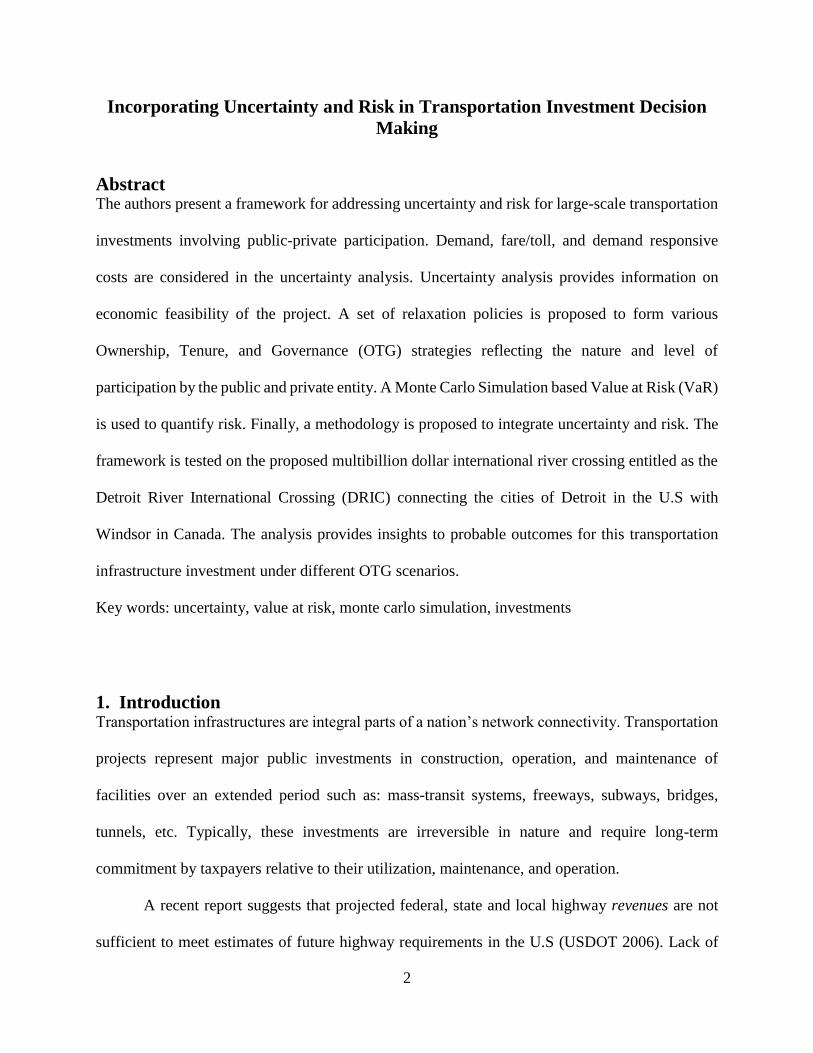
Abstract The authors present a framework for addressing uncertainty and risk for large-scale transportation

investments involving public-private participation. Demand, fare/toll, and demand responsive

costs are considered in the uncertainty analysis. Uncertainty analysis provides information on

economic feasibility of the project. A set of relaxation policies is proposed to form various

Ownership, Tenure, and Governance (OTG) strategies reflecting the nature and level of

participation by the public and private entity. A Monte Carlo Simulation based Value at Risk (VaR)

is used to quantify risk. Finally, a methodology is proposed to integrate uncertainty and risk. The

framework is tested on the proposed multibillion dollar international river crossing entitled as the

Detroit River International Crossing (DRIC) connecting the cities of Detroit in the U.S with

Windsor in Canada. The analysis provides insights to probable outcomes for this transportation

infrastructure investment under different OTG scenarios.

Key words: uncertainty, value at risk, monte carlo simulation, investments

1. Introduction Transportation infrastructures are integral parts of a nation’s network connectivity. Transportation

projects represent major public investments in construction, operation, and maintenance of

facilities over an extended period such as: mass-transit systems, freeways, subways, bridges,

tunnels, etc. Typically, these investments are irreversible in nature and require long-term

commitment by taxpayers relative to their utilization, maintenance, and operation.

A recent report suggests that projected federal, state and local highway revenues are not

sufficient to meet estimates of future highway requirements in the U.S (USDOT 2006). Lack of

3

capital funds to meet the needs of the country may result in increased private participation in

transportation infrastructure projects (Roth 1996). The potential of such projects to produce

economic benefits has become an increasingly important factor in investment decision making.

Such investments may involve the private enterprise in the construction, operation and

maintenance process along with the federal, state and local governments.

In traditional economic analysis, future cash flows are assumed to be fully deterministic in

nature. Thus, these are not designed to account for any risk and uncertainty in the assessment of

future returns. In reality, many of these infrastructure projects are associated with significant

uncertainties stemming from lack of knowledge about future cost and revenue streams. The term

“risk” refers to situations where the decision maker can assign mathematical probabilities to the

randomness relative to future outcomes. In contrast, the term “uncertainty” refers to situations

when this randomness cannot be expressed in terms of mathematical probabilities (Knight 1921).

Significant research on investment decision making under uncertainty and risk is reported

in the fields of economics and financial management. These include theoretical approaches on

capital investment considering the irreversibility of investment decisions and uncertainty of

economic environment (Dixit and Pindyck 1994), actual experience of users and policy makers in

an agent-based approach reflecting network management and financing policies (Zhang et al.

2008), investment decision making for a Build Operate and Transfer (BOT) problem using a multi-

objective genetic algorithm and a mean-variance model for BOT scheme under demand

uncertainty (Chen et al. 2003, Chen et al. 2006), capacity expansion using demand uncertainty and

simulated annealing (Sun and Turnquist 2007) and decision making under uncertainty for highway

development using real options approach (Zhao and Kockelman 2006).

4

2. Problem Statement

The problem investigated in this research relates to the need for a unified approach in

incorporating uncertainty and risk in transportation investment decision making. This paper

presents an analytic framework to explore the implications of a joint ownership of a transportation

infrastructure project, when cost/revenue and demand estimates are subject to significant

uncertainties. A case study is also presented to demonstrate the application of the framework.

The framework explores various forms of joint ownership associated with the public and

private enterprise. There are a number of reasons for the growing trend of private participation in

public projects. These include, the scarcity of fiscal resources at the public sector level, the

perception that the private sector is more efficient in managing large projects, and the advantage

of the public and the private sector jointly sharing risks and uncertainties, thereby reducing

exposure levels to financial losses for both entities. Joint ownership has become increasingly

popular in Europe, Australia and more recently in Asia, as it allows a part or the whole of the

capital funds from private resources in exchange of future revenues (Garber and Hoel 2002,

Khasnabis et al. 2010). Joint ownership is generally associated with three terms: Ownership,

Tenure and Governance (OTG). An OTG strategy can be looked upon as a mechanism to plan,

design, implement, operate, and maintain a project by developing various combinations of

ownership, tenure, and governance procedures, where:

The term ‘Ownership’ has embedded in it, the concept of ‘possession’ and ‘title’ related

to the property in question. Depending upon the nature of the joint project, its ownership

may belong to the public entity, private entity, or both during the concession period.

Ownership may also change at the end of the concession period (Merna and Njiru 1998).

5

‘Tenure’ refers to the status of holding a possession of a project for a specific period,

ranging from few days to a number of years. For most joint ownership projects, tenure is

likely to coincide with the concession period; however, exceptions to this general rule

may be encountered.

‘Governance’ refers to management, policy and decision making pertaining to an

organization with the intent of producing desired results.

The objective of this research is to propose a framework to incorporate uncertainty and risk,

and to evaluate the proposed framework with a real-world case study. The methodology proposed

in the paper is designed for major transportation infrastructure projects involving public private

participation. The case study is applied to an international toll bridge.

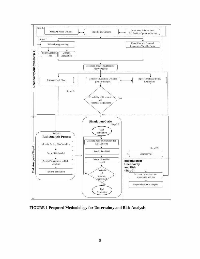
3. A Combined Framework for Uncertainty and Risk Analysis

The proposed framework to incorporate the concept of investment decisions under

uncertainty and risk is illustrated in Figure 1 and is categorized into three steps;

1. Step 1: Uncertainty Analysis

2. Step2: Risk Analysis

3. Step 3: Integration of uncertainty and risk

Step-1: Uncertainty Analysis

Uncertainty analysis is further divided into three sub-steps:

Step - 1.1: Policy Options

Step - 1.2: Bi-level Programming for uncertainty analysis

Step - 1.3: Feasibility Analysis

6

Step 1.1 is an examination of the investment policy options recommended by the relevant

public agencies relating to new transportation projects that may represent various combinations of

rights and responsibilities of public and private agencies (FHWA 2010). At one end of the

spectrum, the public entity may have all the major responsibilities, with the private agency playing

a minor role. At the other end, the roles may be reversed. Various other combinations may form

the intermediate range.

In Step 1.2, a bi-level approach is considered for evaluation of the proposed policy options.

The policy maker (upper level) is assumed to have some understanding of the road users’ likely

response (lower level) to a given strategy. However, the strategy set by the policy maker can only

influence (but not control) the road user behavior relative to choice of routes, modes, etc. In other

words, policy options and choice decisions can be represented as a bi-level program, where, the

upper level involves the policy maker’s decision to determine the toll value, while road users are

assigned to the proposed facility at the lower level. Further, the upper level may involve three

entities (1) private investor, (2) public investor, (3) road user. While the designed toll value for the

three perspectives maybe different at the upper level, a user equilibrium assignment process is

introduced at the lower level with an elastic demand feature designed to consider uncertainty in

travel pattern.

In Step 1.3 economic and financial feasibility of various policy options are examined.

Policy regulations such as construction cost subsidy, concession period extension, etc. can be

considered if necessary. The relaxations are embedded in a set of OTG strategies discussed later.

The viability of the project under different strategies can be tested using a set of pre-specified

criteria.

7

Step - 2: Risk Analysis

Three sub-steps are proposed in the risk analysis:

Step 2.1: Identification of risk variables

Step 2.2: Setting up the simulation process

Step 2.3: Estimation of Value at Risk (VaR)

Variables associated with different investment options are identified in step 2.1. For example, in

transportation investments, possible risk variables are related to demand, fare, and costs.

Probabilities are assigned to the risk variables in a simulation model. A number of simulation

approaches and risk measures are presented in the literature (Jorion 1997). In step 2.2, various

iterations of the simulation cycle are recorded. In step 2.3, a measure of risk is determined. One

such measure is “Value at Risk” (VaR), that can be used to denote the maximum expected loss

over a given horizon at a given confidence level for a specific policy option. This step is designed

to enable the decision maker avoid risky policy options, and to focus more on those options with

modest risk exposure.

8

FIGURE 1 Proposed Methodology for Uncertainty and Risk Analysis

State Policy Options

Bi-level programmingFixed Cost and Demand

Responsive Variable Costs

Measures of Effectiveness for

Policy Options

Estimate Cash Flow Consider Investment Options:

(OTG Strategies)

Impose (or Relax) Policy

Regulations

Feasibility of Economic

and

Financial Regulations

Yes

No

Investment Policies from

Toll Facility Operators SurveyUSDOT Policy Options

Step-1.1

Step-1.2

Step-1.3

Demand

Assignment

Policy Decision

(Toll)

Identify Project Risk Variables

Set up Risk Model

Assign Probabilities to Risk

Variables

Perform Simulation

Recalculate MOE

Record Simulation

Result

Generate Random Numbers for

Risk Variables

Start

Simulation

End

Simulation

Desired #

of

Iterations

Performed

Estimate VaR

Integrate the measures of

uncertainty and risk

Risk Analysis Process

Simulation Cycle

Un

ce

rta

inty

An

aly

sis

(Ste

p-1

)R

isk

An

aly

sis

(Ste

p-2

)

Yes

No

Integration of

Uncertainty and Risk(Step-3)

Propose feasible strategies

Step-2.1

Step-2.2

Step-2.3

9

Step 3: Integration of Uncertainty and Risk

In this step, Measures of Effectiveness (MOE) of uncertainty and risk analyses are combined.

Policy options to address the implications of uncertainty and risk can be proposed for further

consideration.

3.1 Uncertainty Analysis

Sources of uncertainty in the transportation infrastructure investment can arise from lack of

knowledge about future costs and revenues. Bulk of the cost element is from construction cost

incurred before the facility is opened to traffic; other cost elements such as operation and

maintenance costs (regular and periodic) depend on future travel demand. Revenue is directly

dependent on travel demand and toll. Thus, uncertainties related to cost and revenue is primarily

related to travel demand.

Investments in major transportation infrastructure are often complex, with a mix of public

and private finance with the respective agencies having different missions and motivations. The

public sector may consist of national, state and local agencies with a social welfare perspective.

Public and private entities are interested in exploring optimal tolling strategies that may yield

different solutions (Hyman and Mayhew 2008, Wong et al. 2005, Palma et al. 2006, Rouwendal

and Verhoef 2006). While the public entity’s primary interest is to maximize consumer surplus1

(social welfare), the private entity is interested in maximizing profit. Since the public sector is the

eventual owner and operator of the facility, it must ensure that the facility attracts users and serves

the needs of the community (Yang and Meng 2000). Thus, the optimal toll must be viable to the

1 The additional value or benefit received over and above the expenses actually made is known as consumer surplus.

10

ultimate end users. Hence, in the investment decision making process, three entities’ perspectives

should be considered: (1) the private, (2) the public, and (3) the user.

Private Investor’s Perspective

The objective of the private investor is to maximize profit. The annual profit for demand

uncertainty is the difference between benefit and cost and is presented as following (Chen and

Subprasom 2007):

n n nP ,x , B C (1)

Where, Pn is the profit generated in year n, which is a function of the demand (x) and toll

(). Bn and Cn are corresponding revenue and cost for year n respectively. The revenue generated

is a function of uncertain demand and toll, while the cost can be presented in the form of capital

and operation and maintenance cost.

Public Investor’s Perspective

The proposed framework is based on the premise that the primary objective of the public entity is

to maximize consumer surplus, typically measured as the additional monetary value over and

above the price paid (Wohl and Hendrickson 1984). There are other social benefits such as

improved traffic flow, environmental benefits, higher safety etc., that may be derived from major

infrastructure projects. These are not incorporated in the proposed framework and the classical

approach of maximization of consumer surplus was used as the only public benefit.

11

Road User’s Perspective

Ideally, project benefits should be uniformly distributed over the entire study area. If the

project only benefits a small section of travelers in the study area, then the distribution of such

benefits cannot be considered equitable. Theil’s index, one of the commonly used measures of

inequality distribution was used in this study because of its flexible structure (Theil 1967). The

Theil’s Index is considered as a minimization function and is based on the distribution of trips

among TAZs in the study area. Lower values of Theil’s index represent increasing levels of equity

in the distribution of benefits, and vice versa. A zero value of the index indicates a perfect equity

of distribution of benefits across the study area.

While the upper level program determines the toll for various perspectives considered, the

lower level determines the route choice of users for a designed toll value subjected to uncertain

demand. The lower level problem is a user equilibrium traffic assignment with elastic demand

(Sheffi 1985).

Necessary algorithms for maximization of profit for the private sector, for maximization

of consumers’ surplus for the public sector, and minimization of Theil’s Index for the road user

are discussed in detail in the project report (Khasnabis and Mishra 2009). A summarized version

of the formulation is presented in Appendix A.

Demand Elasticity and Uncertainty

Addition of new links or improvement of the road network will reduce the travel cost

between origin and destination. This improvement can result in increasing demand between the

corresponding OD pairs. An exponential demand function can be used to estimate the annual

demand (Sheffi 1985).

12

nn n

rs rsrsq q exp (2)

Where, n

rsq is the random potential demand between r-s,

n

rs is the minimum travel cost between

r-s which includes the designed toll value, is a positive constant, and n

rsq is the realized travel

demand for year n between the OD pair r-s.

Uncertainty in travel demand is incorporated through a random sampling approach with a

predefined mean and variance. Random numbers are generated with a predefined probability

distribution function (i.e. normal distribution). This is performed exogenously from the lower level

traffic assignment (Chen and Subprasom 2007)

n n n

rsrs rsq q z (3)

Where, n

rsq ,

n

rs are the mean and standard deviation of random potential demand for OD pair r-

s, and z is a random variable generated from normal distribution with mean zero and unity variance.

The link travel time used in the lower level traffic assignment problem is the Bureau of Public

Roads function, denoted as (Sheffi 1985):

4

nn n 0 aa a a n

a

xt x t 1 0.15

G

(4)

where, 0

at and aG is the free flow travel time and capacity for link a.

3.2 Risk Analysis

Risk is often defined as the probability of occurrence of an undesirable outcome (Jorion

1997). Risk analysis consists of simulating the various inputs over the life of the project and finding

13

the present value. This process is repeated a number of times using Monte Carlo Simulation (MCS)

to incorporate risks from multiple sources, both on revenues and on costs. The Measure of

Effectiveness (MOE) thus obtained would reflect the effect of risk.

In the proposed risk analysis, the simulation model employs pre-defined realizations of toll

and traffic volume to analyze the effect of indecisive inputs on the output of the modeled system.

Risk can be quantified and measured in different ways (Mun 2006). Value at Risk (VaR) is one

such that can be defined as the maximum expected loss (or the lower value of MOE) over a target

horizon, with a given level of confidence (Jorion 1997). VaR describes a quantile of the projected

distributions of gains and losses over the target horizon. If α is the selected confidence level, VaR

corresponds to the (1- α) lower tail level. For example, for 90 percent confidence level, VaR should

be such that it exceeds 10 percent of the total number of observations in the distribution.

4. Case Study

A proposed international bridge between the city of Detroit in the U.S and the city of

Windsor in Canada is selected as the case study. Surface trade between Southwestern Ontario and

Southeastern Michigan exceeded 200 billion in 2004 and is expected to increase by two-fold by

the year 2030 (MDOT 2003). 70 percent of trade movement between the US and Canada is by

trucks. Approximately 28 percent of surface trading is by trucks for the crossings between

Southeast Michigan and Southwest Ontario (MDOT 2008). Majority of the trade is for the

crossings in the Detroit River area, connecting the city of Detroit in the U.S and the city of Windsor

in Canada. This large trade volume has a significant positive effect on the local, regional and

national economies through cross-border employment opportunities.

14

The Central Business Districts (CBD) of the cities of Detroit and Windsor are currently

connected by four crossings: (1) The Ambassador Bridge (AB), (2) The Detroit Windsor Tunnel

(DWT), (3) a Rail Tunnel (RT), and (4) The Detroit Windsor Truck Ferry (DWTF). Both AB and

DWT are across the Detroit river, built during the late 1920s. AB is a privately owned four-lane

suspension structure, while DWT is a two-lane facility with height restriction, jointly owned by

the two cities and operated by a private corporation. . The RT and DWTF, both constructed under

the Detroit river, carry cargo between two cities. The Blue Water Bridge (BWB) across the St.

Clair River (100 km north of Detroit) that connects the cities of Port Huron in the U.S and Sarnia

in Canada. BWB is a six lane arch structure built in 1938 and renovated in 1999; and is jointly

owned by the two cities.

The Canada–U.S–Ontario–Michigan Transportation Partnership Study (Partnership Study)

attempted to develop long-term strategies to provide safe and efficient movement for people and

goods between Michigan and Ontario (MDOT 2008). Even though the current capacities of the

Ambassador Bridge and the Detroit-Windsor tunnel adequately serve the traffic needs during most

hours, on specific days during peak periods, the systems operates at full capacity. Considering

long-term traffic growth and the overall importance of the Detroit River crossings on the regional

economy, the need for a new crossing seems immensely justified. As a result of number of recent

studies, the Michigan Department of Transportation (MDOT), and the Ontario Ministry of

Transportation have identified a bridge known as X-10(B) as the most preferred alternative to build

in the vicinity of the Ambassador Bridge (MDOT 2008). The alternative has been referred to as

the Detroit River International Crossing (DRIC) in the case study (Figure 2). DRIC, with some

minor adjustments, has recently been renamed as the New International Trade Crossing (NITC)

(Detroit Free Press, 2012). For most up to date information on the case study please refer to the

15

FIGURE 2 Network of Study Area (Mishra 2009)

Blue Water Bridge

Detroit Windsor Tunnel

Entire Network

U.S.

Canada

16

project website2.

5. Results

Two alternative bridge structures are proposed for X-10(B); (1) a suspension bridge, or (2)

a cable-stay bridge. The preliminary cost estimates of the bridges along with associated

infrastructures are $1,809 million and $1,814 million respectively. The cost of $1,814

million includes construction cost of the bridge, toll plaza, access highway with a new

interchange, cost of property acquisition, planning and design (all for the US part of the

project). By the same token, all the toll revenue compiled to assess the benefits reflects the

fare collected at the Detroit end of the bridge that is expected to be open to traffic in the

year 2015.

5.1 Travel Demand Uncertainty

Travel demand data for the study area in the form of origin- destination (OD) matrices for

the study area are obtained from MDOT for the years 2015, 2025, and 2035. There are a

total of 960 Traffic Analysis Zones (TAZ) in the Detroit (U.S) side of the border and 527

TAZs in the Windsor (Canada) side of the border. Including 23 external TAZs, the study

area consists of a total of 1510 TAZs, making for a total of 1510 x 1510 possible

interchanges in the travel demand matrix. The analysis period for the case study is

considered as 35 years (2015-2050). The OD matrix for the year 2045 was projected by

considering the growth trends for each TAZ. A coefficient of variation3 of 0.15 is

2 https://www.michigan.gov/buildthisbridge

3The coefficient of variation (COV) is the ratio of the standard deviation and the mean. For this research a

COV of 0.15 is assumed by observing the variation in demand over time for ten years.

17

considered to incorporate variance in travel demand. A potential4 OD matrix was not

available. The base and horizon year projected OD matrices were increased by ten percent

to obtain the potential OD. The standard deviation of the OD matrix was obtained from the

coefficient of variation and the expected demand of the OD matrix.

Solution Approach for Demand Uncertainty

A Monte Carlo Simulation (MCS) procedure was used to simulate the OD matrix. The

potential OD matrix and the variance OD matrix served as the input to the MCS. The OD

matrices were subjected to 200 realizations and each realization was recorded (Equation

20). From the distribution of OD matrix, the median matrix was chosen for further analysis.

However, one can use any percentile from the distributed OD matrix. This procedure was

followed for all the horizon years. The resulting OD matrix from MCS incorporates the

variation and resulting uncertainties in travel demand, which is used in the elastic traffic

assignment procedure.

The proposed traffic assignment model was calibrated for the base year 2004.

Actual toll values for cars and trucks for the year 2004 are utilized to determine the assigned

volume on the existing river crossings in the network. The proposed elastic traffic

assignment model and the potential OD matrix for the year 2004 are utilized to determine

the assigned volume for cars and trucks. The observed car and truck volumes are obtained

from MDOT (MDOT 2003). The close correspondence between the assigned and observed

volumes at the respective crossings demonstrates the calibration of the model. Results of

4 The potential OD matrix contains the maximum possible trips that can be made if the travelers are not

sensitive to the user cost. In elastic traffic assignment the potential OD matrix is used to test the sensitivity

of demand with respect to the user cost (both travel time and travel cost).

18

the calibration are not presented in the paper for the sake of brevity. The details of

calibration of the model are discussed in the project report (Khasnabis and Mishra 2009).

5.2 Single Entity Perspective Decision Making Under Uncertainty

The objectives of the three entities from investment viewpoint are different, as discussed

earlier. Three entity objectives are used at the upper level and ridership is determined at

the lower level. The bi-level process is solved in TransCAD (Caliper 2008). A GISDK

script is written to solve the bi-level model in TransCAD. The output of the upper level

(toll value and the entity-specific objective function) served as the input to the lower level

(ridership estimation). The bi-level process can be viewed as a non-linear problem

reflecting the nature of the objective functions at the upper and the lower level. The elastic

traffic assignment problem is solved by user equilibrium method using Frank Wolfe

Algorithm (Sheffi 1985).

5.3 Results of Travel Simulation

Results of the travel simulation are presented for the three entities for different horizon

years in Table 1. For the private entity, the objective is profit maximization with the

assumption that the total cost (capital, operation and maintenance cost) will be borne by

the private entity. Revenue is considered as a surrogate for profit in this paper. As

explained earlier, the optimization processes for the three entities were solved by the bi-

level approach. Toll values are set at the upper level and ridership is determined at the

lower level. The toll values are obtained in an iterative manner with directional search5 to

5 Directional search is a technique for finding the optimal value of a unimodal function by successively

narrowing from the possible range of values.

19

obtain the optimum value of the objective function for profit maximization, consumer

surplus maximization and inequality minimization.

For example, in the profit maximization strategy, optimal toll values of $2 per car and $14

per truck resulted in annual revenue6 of $68.54 million in the year 2015. For the same toll

values the consumer surplus and Theil’s index are estimated to be $346.07 million and 0.86

respectively for the year 2015. The last two numbers are not, however, optimal values as

explained below.

When objective of the public entity is considered, the optimal toll is $0.5 per car

and $4.33 per truck (year 2015, second row, Table 1) that resulted in an optimal consumer

surplus of $730.36 million, which is higher than the estimated consumer surplus for profit

maximization. The consumer surplus allows more travelers7 to use the facility in lowering

the difference between willingness to pay and what the travelers actually pay. The revenue

and Theil’s index for toll value of $0.5 for cars and $4.33 for trucks are estimated to be

$25.78 million and 0.79 respectively (Non-optimal).

Similarly, when the perspective of the users is considered (year 2015, third row,

Table 1) the optimal toll values obtained are $0.25 per car and $ 1.04 per truck, resulting

in a Theil’s index of 0.70 (minimum of the three Theil’s index values) for the year 2015.

For the toll value of $0.25 per car and $ 1.04 per truck the corresponding revenue and

consumer surplus are estimated at $7.41 and $258.62 million respectively (Non-optimal).

6 Revenue is defined as the monetary benefit obtained by the toll/fare collection only and for a specific year

where as profit is for the analysis period.

7 It should be noted that more travelers using the facility do not necessarily increase the revenue, because

revenue is the product of toll value and the corresponding ridership.

20

TABLE Travel 1 Simulation Results (25) Year Car Toll

($)

Truck Toll

($)

Annual

Revenue

(Million $)

Annual

Consumer

Surplus

(Million $)

Theil’s

Inequalit

y Index

2015

Private Perspective 28 149 68.5410 346.07 0.86

Public Perspective 0.511 4.3312 25.78 730.3613 0.79

User Perspective 0.2514 1.0415 7.412 258.62 0.7016

2025

Private Perspective 3 15 118.22 550.98 0.88



2035

Private Perspective 4.5 19 199.30 681.45 0.88



2045

Private Perspective 6.00 21.00 281.95 802.24 0.86



2050

Private Perspective 8.73 22.25 330.63 936.19 0.88



Three distinct toll values are obtained for three different entities, each of which

represents the optimum values for the three objective functions defined in equations 6, 12,

and 15 in Appendix A. The highest toll value resulted for profit maximization and the least

8 Represents the Optimal value of car toll from the Private Perspective 9 Represents the Optimal value of truck toll from the Private Perspective 10 Represents the maximum value of Revenue from the Private Perspective 11 Represents the Optimal value of car toll from the Public Perspective 12 Represents the Optimal value of truck toll from the Public Perspective 13 Represents the maximum value of Consumer Surplus from the Public Perspective 14 Represents the Optimal value of car toll from the User Perspective 15 Represents the Optimal value of truck toll from the User Perspective 16 Represents the minimum value of Theil’s value from the User Perspective

21

toll value for Theil’s Index, thereby demonstrating that the objectives of the private

investor and the users are satisfied. Additionally, the toll value for the public entity

perspective is lower than that for the private perspective for all the years. Similar trends

are observed for the other horizon years during the analysis period presented in Table 1.

Increased travel demand in future years resulted in higher toll values, higher revenue and

higher consumer surplus in succeeding years. The same is generally true fort Theil’s Index,

although there are some exceptions.

5.4 Ownership, Tenure and Governance Strategies

The authors’ initial work on the concept of OTG scenarios was presented at the World

Conference on Transport Research at the University of California, Berkeley in 2007

(Khasnabis et al. 2007). Though single entity participation in large transportation projects

is important, their involvement with other entities is likely to increase the overall viability

of the project. Ownership, Tenure and Governance (OTG) are the three principal

components of joint ownership (Mishra et al. 2013; Mishra et al. 2014).

A number of OTG strategies are considered to represent varying levels and types

of public-private participation in the DRIC project. The strategies vary in the degree of

participation by the public and the private entity. Five types of OTG strategies are

considered:

1. OTG-1: Exclusive Private Participation

2. OTG-2: Major Private Participation

3. OTG-3: Moderate Private Participation

4. OTG-4: Major Public Participation

5. OTG-5: Exclusive Public Participation

22

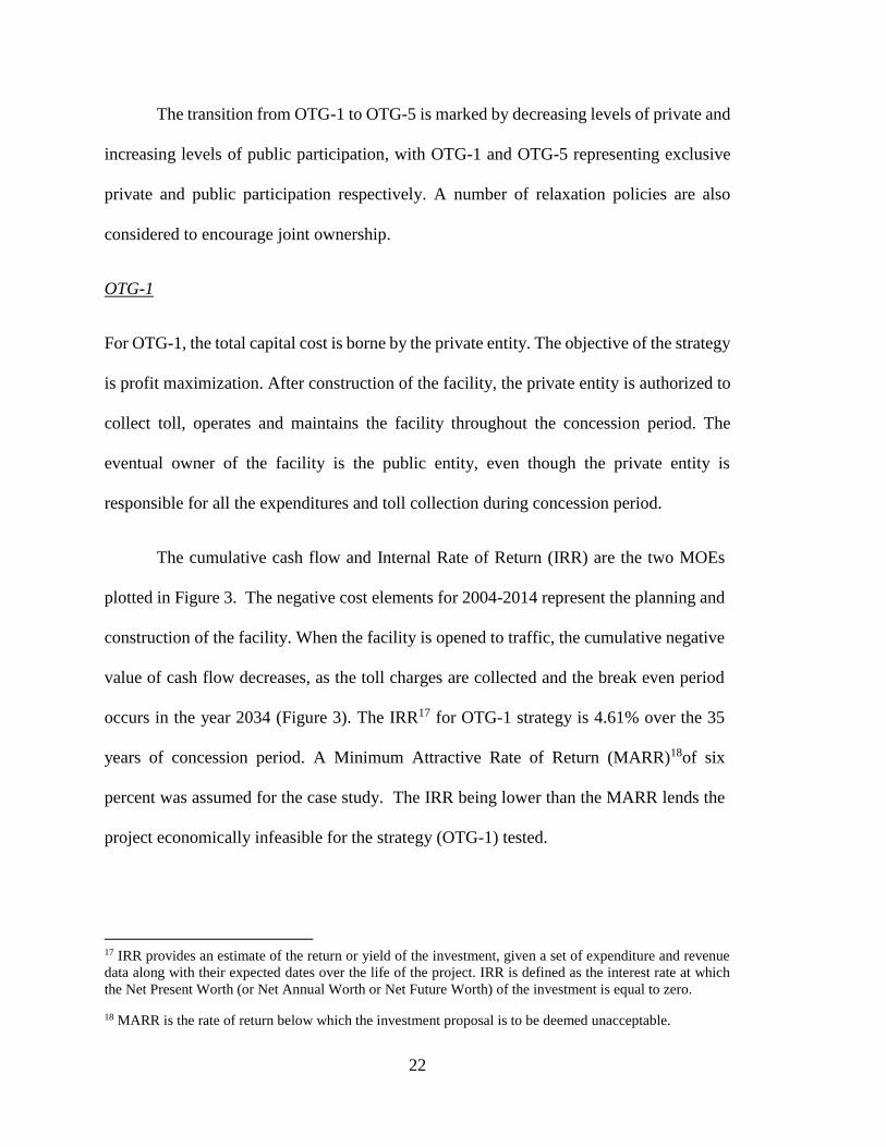
The transition from OTG-1 to OTG-5 is marked by decreasing levels of private and

increasing levels of public participation, with OTG-1 and OTG-5 representing exclusive

private and public participation respectively. A number of relaxation policies are also

considered to encourage joint ownership.

OTG-1

For OTG-1, the total capital cost is borne by the private entity. The objective of the strategy

is profit maximization. After construction of the facility, the private entity is authorized to

collect toll, operates and maintains the facility throughout the concession period. The

eventual owner of the facility is the public entity, even though the private entity is

responsible for all the expenditures and toll collection during concession period.

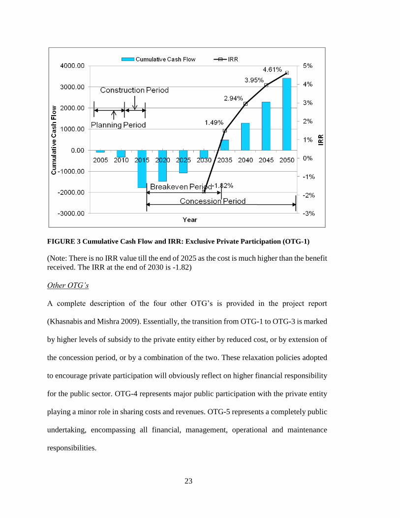
The cumulative cash flow and Internal Rate of Return (IRR) are the two MOEs

plotted in Figure 3. The negative cost elements for 2004-2014 represent the planning and

construction of the facility. When the facility is opened to traffic, the cumulative negative

value of cash flow decreases, as the toll charges are collected and the break even period

occurs in the year 2034 (Figure 3). The IRR17 for OTG-1 strategy is 4.61% over the 35

years of concession period. A Minimum Attractive Rate of Return (MARR)18of six

percent was assumed for the case study. The IRR being lower than the MARR lends the

project economically infeasible for the strategy (OTG-1) tested.

17 IRR provides an estimate of the return or yield of the investment, given a set of expenditure and revenue

data along with their expected dates over the life of the project. IRR is defined as the interest rate at which

the Net Present Worth (or Net Annual Worth or Net Future Worth) of the investment is equal to zero.

18 MARR is the rate of return below which the investment proposal is to be deemed unacceptable.

23

FIGURE 3 Cumulative Cash Flow and IRR: Exclusive Private Participation (OTG-1)

(Note: There is no IRR value till the end of 2025 as the cost is much higher than the benefit

received. The IRR at the end of 2030 is -1.82)

Other OTG’s

A complete description of the four other OTG’s is provided in the project report

(Khasnabis and Mishra 2009). Essentially, the transition from OTG-1 to OTG-3 is marked

by higher levels of subsidy to the private entity either by reduced cost, or by extension of

the concession period, or by a combination of the two. These relaxation policies adopted

to encourage private participation will obviously reflect on higher financial responsibility

for the public sector. OTG-4 represents major public participation with the private entity

playing a minor role in sharing costs and revenues. OTG-5 represents a completely public

undertaking, encompassing all financial, management, operational and maintenance

responsibilities.

24

TABLE 2 OTG Strategies, Relaxation Policies and IRR’s

OTG

Strategy

Explanation Relaxation Policy Entity

Objective

IRR (%)

(Private)

IRR (%)

(Public)

OTG-1 Exclusive

Private

Participation

1. No Relaxation Profit

Maximization

4.61

OTG-2 Major Private

Participation

2(a). Toll Plaza Cost Subsidy

2(b). Toll Plaza, Interchange, and

Inspection Plaza Cost Subsidy

2(c). Construction Cost Subsidy

Profit

Maximization

5.14

5.89

5.84

OTG-3 Moderate

Private

Participation

3(a). Construction Cost Subsidy

3(b). Concession Period Extension

3(c). Construction Cost Subsidy and

Concession Period Extension

Profit

Maximization

6.13

6.01

7.20

OTG-4 Major Public

Participation

4(a). Partly Construction Cost by

Private Entity

4(b) Operation and Maintenance Cost

–Public Entity

4(c). Construction Cost Subsidy-

Public Entity

Consumer

Surplus

Maximization

22.97*

3.27**

3.69**

3.95**

OTG-5 Exclusive

Public

Participation

No Relaxation Consumer

Surplus Max.

3.51**

Note: *: Private entity is only responsible for a part of the construction cost and receives all the benefits throughout the concession

period. Lesser investment and higher return for the private entity has resulted in relatively larger IRR. This OTG strategy is considered

as an attractive option for the private entity.**: IRR for the public entity (the remainder of the IRR are for the private entity).

25

Synthesis of Results for OTG Strategies

The objective of OTG strategy analysis is to assess the fiscal impact of varying levels of

joint ownership scenarios on the public and the private entities.OTG-1 and OTG-5

represent exclusive private and public projects respectively (with no role by the other

agency) as the two ends of the joint participation spectrum. OTG-2 and OTG-3 represent

various levels of relaxation policies designed to provide higher levels of subsidies to the

private agency with all the revenue committed to the agency. OTG-4 is a major public

program with minor participation by the private agency both in cost and revenue sharing.

Results of this analysis are presented in Table2 and can be summarized as follows:

For exclusive private participation (OTG-1), the project is not financially viable,

as the IRR generated (4.61 percent) is lower than the MARR (6.0 percent).

Further, varying degrees of relaxation are proposed in (OTG-2 and OTG-3) to

encourage private participation. None of the three relaxation policies within OTG-

2 resulted in IRR values higher than the MARR (6%). On the other hand, all of the

four relaxation policies in OTG-3 resulted in financially viable solutions with IRR

values exceeding the MARR (6%). The exceedingly high IRR (22.97 percent) for

OTG-3(d) is caused by a very large construction cost subsidy to the private agency.

For major and exclusive public participation (OTG-4 and OTG-5), the project is

not financially viable, with none of the IRR values exceeding the 6 percent mark.

OTG-4(a) and 4(b) represent small amounts of costs and revenue sharing by the

private agency with the public agency having the major financial responsibility.

OTG-5, on the other hand, is exclusive public participation and is not financially

viable.

26

In summary, the OTG strategies representing different joint ownership scenarios

generate varying returns ranging from a low of 4.61 percent to a high of 22.97

percent to the private agency, and from 3.27 percent to 3.69 percent for the public

agency. With an assumed MARR of 6 percent, all the four options within OTG-3

are found financially viable for the private agency. Unfortunately, none of the two

options in OTG-4, and the single option in OTG-5 is financially viable for the

public agency.

The implication of the above finding (that the project is not financially viable, with

the public agency sharing most of the fiscal responsibility using the MARR

criterion) needs additional discussion, even though this is somewhat irrelevant to

the focus of the paper, incorporation of uncertainty and risk in investment decision.

Recalling that the only revenue considered in the analysis is the toll collection, one

might argue that the real benefit of such a project to the public at-large manifests

itself in the form of “intangibles” such as: increased mobility, improved safety,

higher levels of comfort and reduced emissions. Further, for most highway projects

supported by taxpayers, no such revenue is ever collected, and only toll roads are

an exception in this regard, because of the funding mechanism. For large-scale

transit projects funded by tax dollars, the fare-box revenue typically covers a

portion of the operating cost, and there is no “payback” program for the capital

cost. Thus, one might further contend that an IRR of 3.51 percent for OTG-5 based

upon toll collection alone, should be considered an acceptable return, even though

it is lower than the MARR of 6 percent. Alternatively, the above mentioned

“intangibles” should be duly incorporated in the analysis. This topic can be a

27

subject of future research.

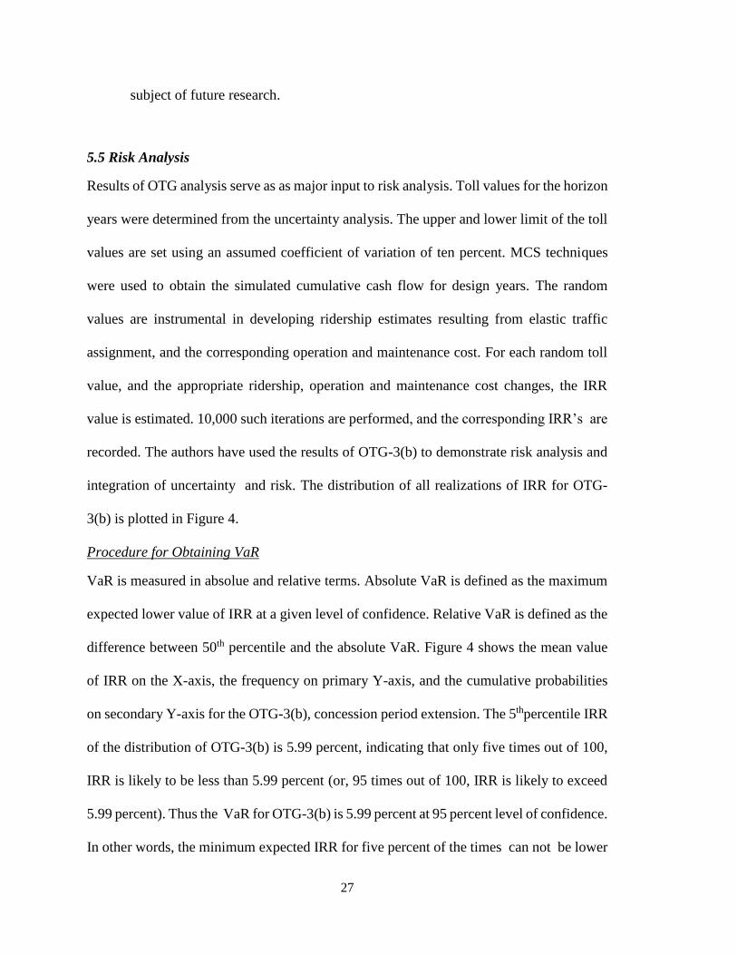
5.5 Risk Analysis

Results of OTG analysis serve as as major input to risk analysis. Toll values for the horizon

years were determined from the uncertainty analysis. The upper and lower limit of the toll

values are set using an assumed coefficient of variation of ten percent. MCS techniques

were used to obtain the simulated cumulative cash flow for design years. The random

values are instrumental in developing ridership estimates resulting from elastic traffic

assignment, and the corresponding operation and maintenance cost. For each random toll

value, and the appropriate ridership, operation and maintenance cost changes, the IRR

value is estimated. 10,000 such iterations are performed, and the corresponding IRR’s are

recorded. The authors have used the results of OTG-3(b) to demonstrate risk analysis and

integration of uncertainty and risk. The distribution of all realizations of IRR for OTG-

3(b) is plotted in Figure 4.

Procedure for Obtaining VaR

VaR is measured in absolue and relative terms. Absolute VaR is defined as the maximum

expected lower value of IRR at a given level of confidence. Relative VaR is defined as the

difference between 50th percentile and the absolute VaR. Figure 4 shows the mean value

of IRR on the X-axis, the frequency on primary Y-axis, and the cumulative probabilities

on secondary Y-axis for the OTG-3(b), concession period extension. The 5thpercentile IRR

of the distribution of OTG-3(b) is 5.99 percent, indicating that only five times out of 100,

IRR is likely to be less than 5.99 percent (or, 95 times out of 100, IRR is likely to exceed

5.99 percent). Thus the VaR for OTG-3(b) is 5.99 percent at 95 percent level of confidence.

In other words, the minimum expected IRR for five percent of the times can not be lower

28

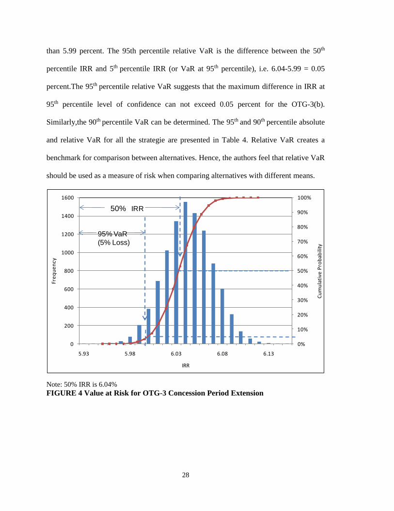
than 5.99 percent. The 95th percentile relative VaR is the difference between the 50th

percentile IRR and 5th percentile IRR (or VaR at 95th percentile), i.e. 6.04-5.99 = 0.05

percent.The 95th percentile relative VaR suggests that the maximum difference in IRR at

95th percentile level of confidence can not exceed 0.05 percent for the OTG-3(b).

Similarly,the 90th percentile VaR can be determined. The 95th and 90th percentile absolute

and relative VaR for all the strategie are presented in Table 4. Relative VaR creates a

benchmark for comparison between alternatives. Hence, the authors feel that relative VaR

should be used as a measure of risk when comparing alternatives with different means.

Note: 50% IRR is 6.04%

FIGURE 4 Value at Risk for OTG-3 Concession Period Extension

0%

10%

20%

30%

40%

50%

60%

70%

80%

90%

100%

0

200

400

600

800

1000

1200

1400

1600

5.93 5.98 6.03 6.08 6.13

Cu

mu

lati

ve P

rob

abili

ty

Fre

qu

en

cy

IRR

Mean IRR

95% VaR

(5% Loss)

50%

29

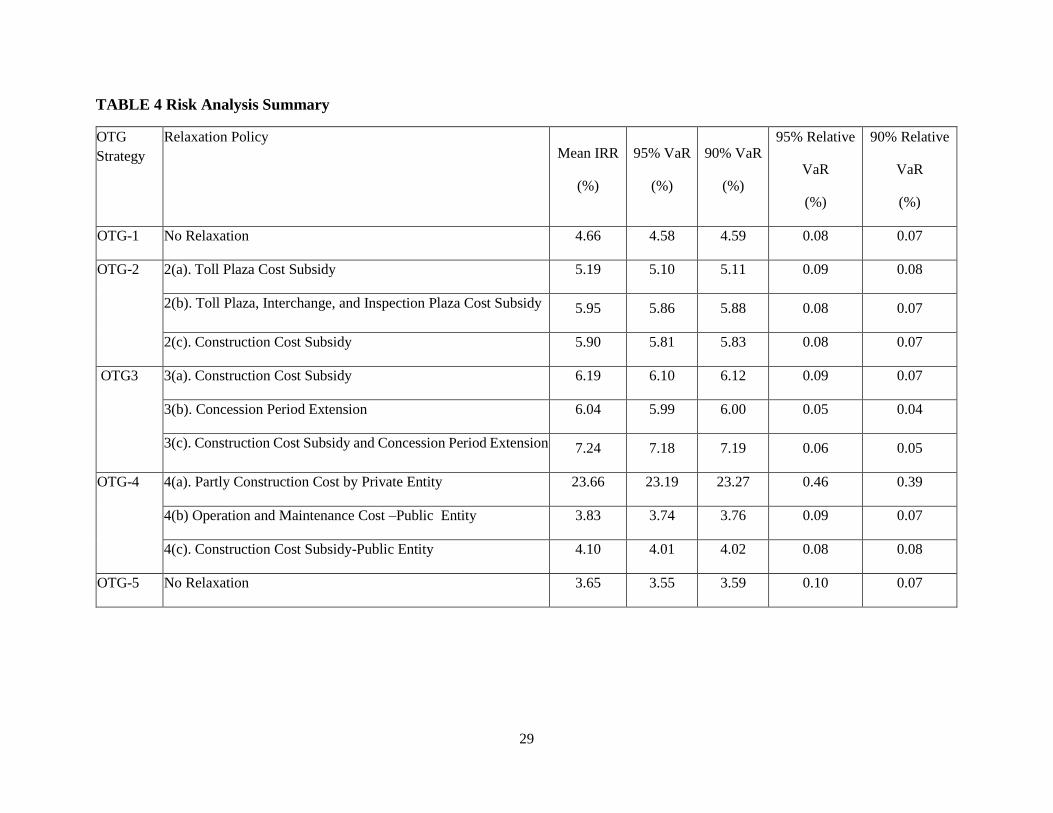
TABLE 4 Risk Analysis Summary

OTG

Strategy

Relaxation Policy Mean IRR

(%)

95% VaR

(%)

90% VaR

(%)

95% Relative

VaR

(%)

90% Relative

VaR

(%)

OTG-1 No Relaxation 4.66 4.58 4.59 0.08 0.07

OTG-2 2(a). Toll Plaza Cost Subsidy 5.19 5.10 5.11 0.09 0.08

2(b). Toll Plaza, Interchange, and Inspection Plaza Cost Subsidy 5.95 5.86 5.88 0.08 0.07

2(c). Construction Cost Subsidy 5.90 5.81 5.83 0.08 0.07

OTG3 3(a). Construction Cost Subsidy 6.19 6.10 6.12 0.09 0.07

3(b). Concession Period Extension 6.04 5.99 6.00 0.05 0.04

3(c). Construction Cost Subsidy and Concession Period Extension 7.24 7.18 7.19 0.06 0.05

OTG-4 4(a). Partly Construction Cost by Private Entity 23.66 23.19 23.27 0.46 0.39

4(b) Operation and Maintenance Cost –Public Entity 3.83 3.74 3.76 0.09 0.07

4(c). Construction Cost Subsidy-Public Entity 4.10 4.01 4.02 0.08 0.08

OTG-5 No Relaxation 3.65 3.55 3.59 0.10 0.07

30

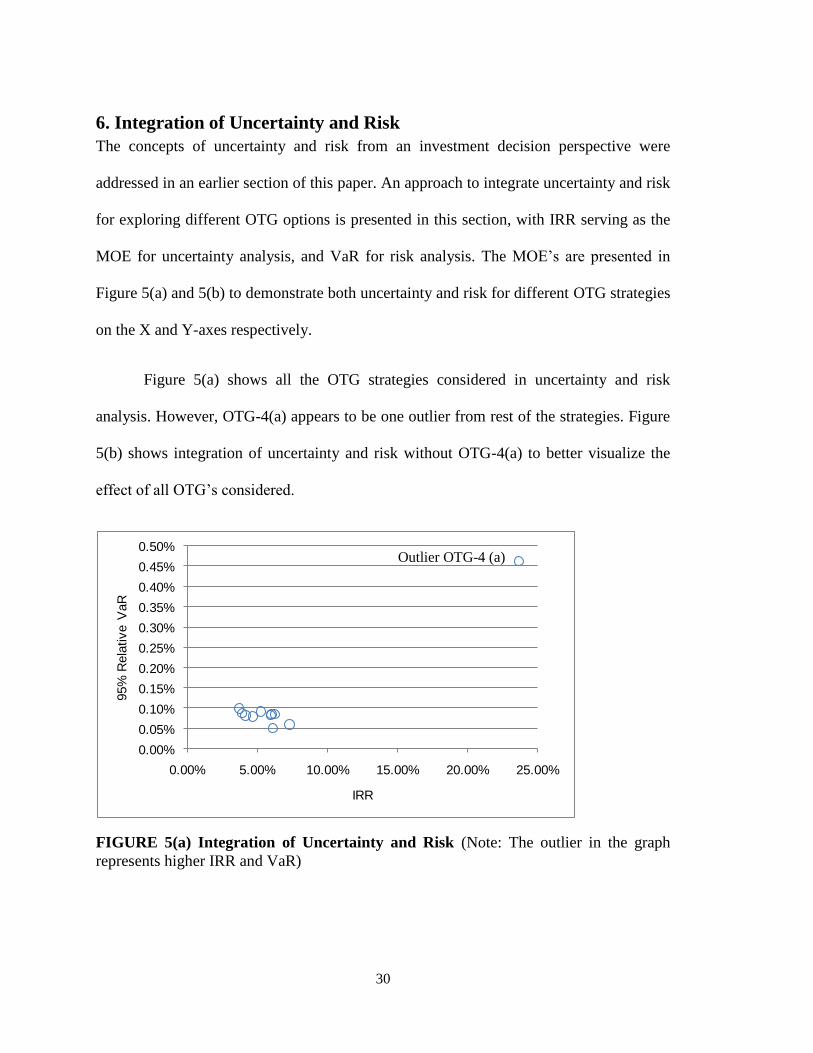
6. Integration of Uncertainty and Risk

The concepts of uncertainty and risk from an investment decision perspective were

addressed in an earlier section of this paper. An approach to integrate uncertainty and risk

for exploring different OTG options is presented in this section, with IRR serving as the

MOE for uncertainty analysis, and VaR for risk analysis. The MOE’s are presented in

Figure 5(a) and 5(b) to demonstrate both uncertainty and risk for different OTG strategies

on the X and Y-axes respectively.

Figure 5(a) shows all the OTG strategies considered in uncertainty and risk

analysis. However, OTG-4(a) appears to be one outlier from rest of the strategies. Figure

5(b) shows integration of uncertainty and risk without OTG-4(a) to better visualize the

effect of all OTG’s considered.

FIGURE 5(a) Integration of Uncertainty and Risk (Note: The outlier in the graph

represents higher IRR and VaR)

0.00%

0.05%

0.10%

0.15%

0.20%

0.25%

0.30%

0.35%

0.40%

0.45%

0.50%

0.00% 5.00% 10.00% 15.00% 20.00% 25.00%

95%

Rela

tive V

aR

IRR

Outlier OTG-4 (a)

31

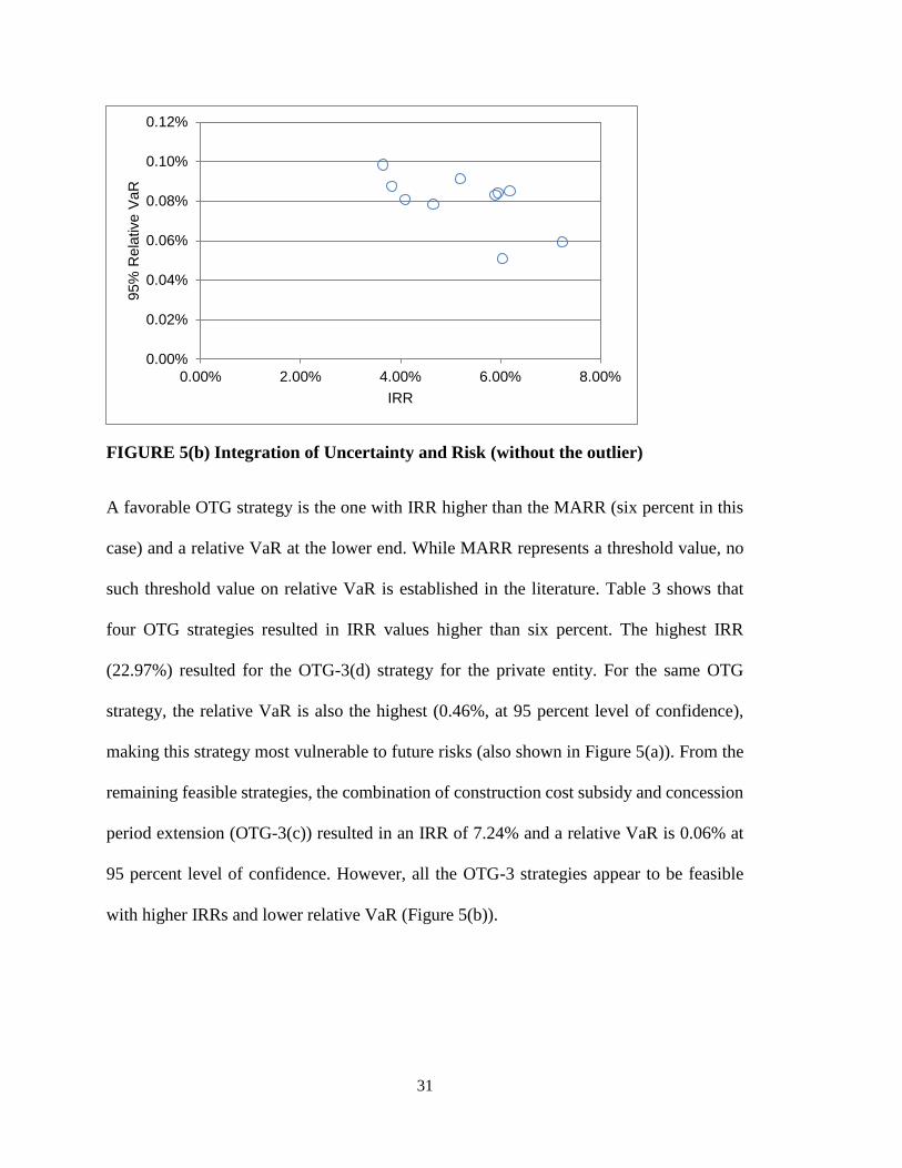
FIGURE 5(b) Integration of Uncertainty and Risk (without the outlier)

A favorable OTG strategy is the one with IRR higher than the MARR (six percent in this

case) and a relative VaR at the lower end. While MARR represents a threshold value, no

such threshold value on relative VaR is established in the literature. Table 3 shows that

four OTG strategies resulted in IRR values higher than six percent. The highest IRR

(22.97%) resulted for the OTG-3(d) strategy for the private entity. For the same OTG

strategy, the relative VaR is also the highest (0.46%, at 95 percent level of confidence),

making this strategy most vulnerable to future risks (also shown in Figure 5(a)). From the

remaining feasible strategies, the combination of construction cost subsidy and concession

period extension (OTG-3(c)) resulted in an IRR of 7.24% and a relative VaR is 0.06% at

95 percent level of confidence. However, all the OTG-3 strategies appear to be feasible

with higher IRRs and lower relative VaR (Figure 5(b)).

0.00%

0.02%

0.04%

0.06%

0.08%

0.10%

0.12%

0.00% 2.00% 4.00% 6.00% 8.00%

95%

Rela

tive V

aR

IRR

32

7. Conclusions

The primary objective of this study is to develop a framework to incorporate the concept

of uncertainties and risks in transportation investment decisions; and to apply the

framework on a real-world case-study to augment the decision making process. The entities

often involved in, or affected by such investment decision are enlisted as: private, public,

and users, each with different set of objectives and expectations; profit maximization,

consumer surplus maximization and inequality minimization, respectively. A procedure

for a single entity uncertainty analysis is presented as a bi-level process. The upper level

constitutes the preference of the policy maker, and the lower level determines the user’s

response to the policy. The output of uncertainty analysis serves as an input to risk analysis.

IRR and VaR are considered as the MOE’s for uncertainty and risk analysis respectively

and determined using MCS techniques. The objective of each entity, when subjected to

uncertainty, is considered in assessing the optimal demand and toll estimates.

Typically, economic analysis of infrastructure projects are based upon the

assumption of deterministic cash flows using the premise that all future costs and revenues

are fully “known”. In reality, there are significant uncertainties stemming from the lack of

knowledge about the future cash flow streams. The picture is further complicated by the

fact that transportation projects are typically long-term in nature, and that “the longer the

project, the higher the uncertainty”. The proposed framework is an attempt by the authors

to address the effect of uncertainty and risk on transportation investment decisions.

Uncertainty analysis can be used to determine the optimal value of the entity-

specific objective function (profit maximization or welfare maximization or inequality

minimization) in a joint ownership project in the face of variable travel demand, toll,

33

operation and maintenance costs. With no prior information on demand, toll, and cost, a

deterministic analysis can result into misleading conclusions, whereas uncertainty analysis

determines the optimal results from each entity perspective. Further, risk analysis considers

inputs from uncertainty analysis to determine the maximum expected lower value of MOE

at a given level of confidence.

If the single entity uncertainty analysis does not result in feasible solutions,

relaxation policies are proposed. Relaxation policies may include extension of the

concession period and financial support from the other entities involved in the decision

making process leading to the formulation of different OTG strategies to reflect multi-

entity operation of the proposed facility and various relaxation policies.

IRR is considered as the measure of feasibility for uncertainty analysis. Similarly,

VaR is recommended as a measure of risk analysis. A methodology for integrating

uncertainty and risk is proposed. It is observed that projects producing higher IRR may

also be associated with higher VaR. The integration of uncertainty and risk allows the

decision maker to choose from a set of alternative investment strategies to minimize

uncertainty and risk, subject to the IRR meeting the MARR criterion. The concept of

integrating uncertainties and risks demonstrated the need to consider not only the return on

the investment (IRR) in the decision making process, but also the risk factor (VaR). The

final decision should be based upon the joint consideration of both factors. Ideally, the

alternative with the highest IRR (provided it is higher than the MARR), and with the

minimum relative VaR is the most desired one.

The framework is applied to study the investment decision making of DRIC

connecting two countries US, and Canada; a project in the planning stage for over ten years.

34

Results of the case study indicate that the framework presented is viable; however

additional research is needed to integrate the perspectives of all the entities into a multi-

objective framework. The case study presented clearly demonstrates that a strategy

considered economically viable under deterministic scenario, may not be so when risk

factors are incorporated in the analysis. As another future task, the effect of changes in the

toll structure of the competing bridges on DRIC can be incorporated into the uncertainty

and risk analysis framework. The proposed procedure may be used by transportation and

financing professionals involved in infrastructure investment decisions. Such professionals

include: engineers/planners/economists, investment and cost analysts involved both in

private and public financing of infrastructure projects.

35

Acknowledgement

This research was supported by the U.S. Department of Transportation (USDOT) through

its University Transportation Center (UTC) program. The authors would like to thank the

USDOT and the University of Toledo for supporting this research through the UTC

program, and Wayne State University (WSU) for providing crucial matching support. The

authors would like to acknowledge the assistance of Michigan Department of

Transportation (MDOT) and Southeast Michigan Council of Governments (SEMCOG) for

their assistance during the course of the study. Lastly, the authors are immensely grateful

to the WSU Center for Legal Studies for supporting the preliminary research on this topic

in 2004-2006 (Khasnabis et al;. 2007). The comments and opinions expressed in this report

are entirely those of the authors, and do not necessarily reflect the programs and policies

of any of the agencies mentioned above.

36

Appendix

Private Investor’s Perspective

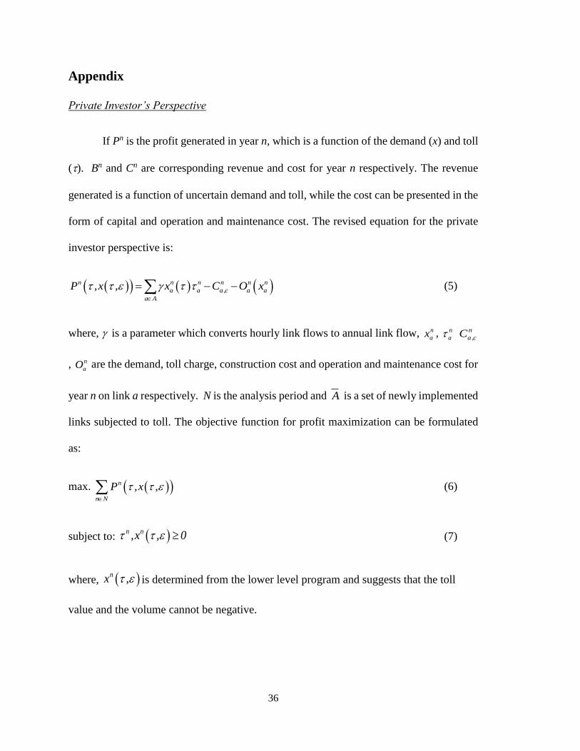
If Pn is the profit generated in year n, which is a function of the demand (x) and toll

(). Bn and Cn are corresponding revenue and cost for year n respectively. The revenue

generated is a function of uncertain demand and toll, while the cost can be presented in the

form of capital and operation and maintenance cost. The revised equation for the private

investor perspective is:

n n n n n n

a a a,c a a

a A

P ,x , x C O x

(5)

where, is a parameter which converts hourly link flows to annual link flow, n

ax , n

a n

a ,cC

, n

aO are the demand, toll charge, construction cost and operation and maintenance cost for

year n on link a respectively. N is the analysis period and A is a set of newly implemented

links subjected to toll. The objective function for profit maximization can be formulated

as:

max. n

n N

P ,x ,

(6)

subject to: n n,x , 0 (7)

where, nx , is determined from the lower level program and suggests that the toll

value and the volume cannot be negative.

37

Public Investor’s Perspective

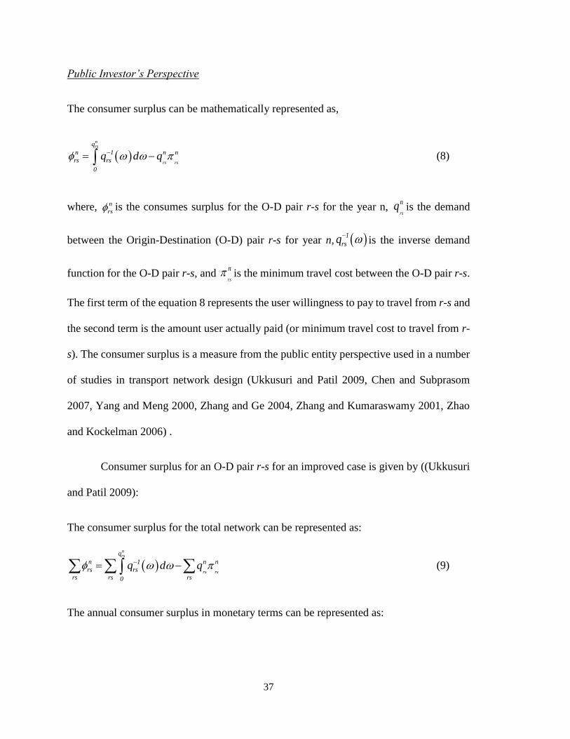
The consumer surplus can be mathematically represented as,

nrs

rs rs

q

n 1 n n

rs rs

0

q d q (8)

where, n

rs is the consumes surplus for the O-D pair r-s for the year n, rs

nq is the demand

between the Origin-Destination (O-D) pair r-s for year n, 1

rsq is the inverse demand

function for the O-D pair r-s, and rs

n is the minimum travel cost between the O-D pair r-s.

The first term of the equation 8 represents the user willingness to pay to travel from r-s and

the second term is the amount user actually paid (or minimum travel cost to travel from r-

s). The consumer surplus is a measure from the public entity perspective used in a number

of studies in transport network design (Ukkusuri and Patil 2009, Chen and Subprasom

2007, Yang and Meng 2000, Zhang and Ge 2004, Zhang and Kumaraswamy 2001, Zhao

and Kockelman 2006) .

Consumer surplus for an O-D pair r-s for an improved case is given by ((Ukkusuri

and Patil 2009):

The consumer surplus for the total network can be represented as:

nrs

rs rs

q

n 1 n n

rs rs

rs rs rs0

q d q (9)

The annual consumer surplus in monetary terms can be represented as:

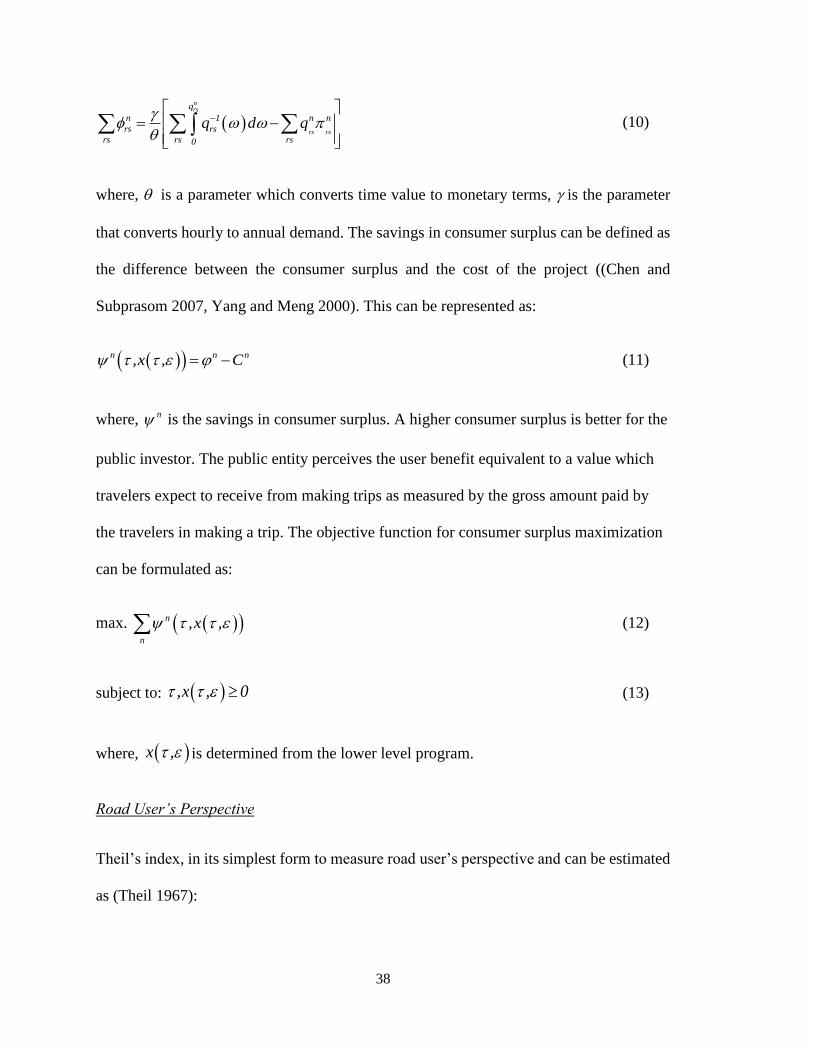
38

nrs

rs rs

q

n 1 n n

rs rs

rs rs rs0

q d q

(10)

where, is a parameter which converts time value to monetary terms, is the parameter

that converts hourly to annual demand. The savings in consumer surplus can be defined as

the difference between the consumer surplus and the cost of the project ((Chen and

Subprasom 2007, Yang and Meng 2000). This can be represented as:

n n n,x , C (11)

where, n is the savings in consumer surplus. A higher consumer surplus is better for the

public investor. The public entity perceives the user benefit equivalent to a value which

travelers expect to receive from making trips as measured by the gross amount paid by

the travelers in making a trip. The objective function for consumer surplus maximization

can be formulated as:

max. n

n

,x , (12)

subject to: ,x , 0 (13)

where, x , is determined from the lower level program.

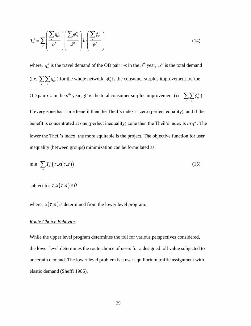
Road User’s Perspective

Theil’s index, in its simplest form to measure road user’s perspective and can be estimated

as (Theil 1967):

39

n n n

rs rs rsn s s s

b n n nr

q

T . .lnq

(14)

where, n

rsq is the travel demand of the OD pair r-s in the nth year, nq is the total demand

(i.e. n

rs

r s

q ) for the whole network, n

rs is the consumer surplus improvement for the

OD pair r-s in the nth year, n is the total consumer surplus improvement (i.e. n

rs

r s

) .

If every zone has same benefit then the Theil’s index is zero (perfect equality), and if the

benefit is concentrated at one (perfect inequality) zone then the Theil’s index is ln nq . The

lower the Theil’s index, the more equitable is the project. The objective function for user

inequality (between groups) minimization can be formulated as:

min. n

b

n

T ,x , (15)

subject to: ,x , 0

where, x , is determined from the lower level program.

Route Choice Behavior

While the upper level program determines the toll for various perspectives considered,

the lower level determines the route choice of users for a designed toll value subjected to

uncertain demand. The lower level problem is a user equilibrium traffic assignment with

elastic demand (Sheffi 1985).

40

a a rsx x q

1

a a rsx ,

rsa Aa A A 0 0 0

min t w dw t w dw q w dw

(16)

subject to:

rs

k rs

k

f q (17)

rs

kf 0 (18)

rsq 0 (19)

rs rs

a k a,k

r s k

x f (20)

if link is on path between O-D

Otherwise

rs

a,k

1 a k r - s

0

(21)

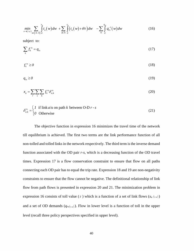
The objective function in expression 16 minimizes the travel time of the network

till equilibrium is achieved. The first two terms are the link performance function of all

non-tolled and tolled links in the network respectively. The third term is the inverse demand

function associated with the OD pair r-s, which is a decreasing function of the OD travel

times. Expression 17 is a flow conservation constraint to ensure that flow on all paths

connecting each OD pair has to equal the trip rate. Expression 18 and 19 are non-negativity

constraints to ensure that the flow cannot be negative. The definitional relationship of link

flow from path flows is presented in expression 20 and 21. The minimization problem in

expression 16 consists of toll value ( ) which is a function of a set of link flows (xa , )

and a set of OD demands (qrs , ). Flow in lower level is a function of toll in the upper

level (recall three policy perspectives specified in upper level).

41

References BTS (2008) '« Transportation statistics annual Report 1999»', US Department of

Transportation, Bureau of Transportation Statistics, Washington.

Caliper, C. (2008) Travel Demand Modeling with TransCAD, email to [accessed

Chen, A. and Subprasom, K. (2007) 'Analysis of regulation and policy of private toll roads

in a build-operate-transfer scheme under demand uncertainty', Transportation

Research Part A, 41(6), 537-558.

Chen, A., Subprasom, K. and Ji, Z. (2003) 'Mean-Variance Model for the Build-Operate-

Transfer Scheme Under Demand Uncertainty', Transportation Research Record,

1857(-1), 93-101.

Chen, A., Subprasom, K. and Ji, Z. W. (2006) 'A simulation-based multi-objective genetic

algorithm (SMOGA) procedure for BOT network design problem', Optimization

and Engineering, 7(3), 225-247.

Detroit Free Press. 2012. New bridge over Detroit River to Windsor could take 7 years to

complete. Detroit Free Press News, December 25, 2012, Detroit, Michigan, USA.

Dixit, A. K. and Pindyck, R. S. (1994) Investment under uncertainty, Princeton University

Press Princeton, NJ.

FHWA (2010) 'Public Private Partnership', [online], available: [accessed

Garber, N. and Hoel, L. (2002) 'Traffic and Highway Engineering. Brooks/Cole',

Hyman, G. and Mayhew, L. (2008) 'Toll optimisation on river crossings serving large

cities', Transportation Research Part A, 42(1), 28-47.

Johnson, C. L., Luby, M.J., and Kurbanov, S.I (2007) 'Toll Road Privatization

Transactions: The Chicago Skyway and Indiana Toll Road', [online], available:

http://www.cviog.uga.edu/services/research/abfm/johnson.pdf [accessed

Jorion, P. (1997) Value at risk: the new benchmark for controlling market risk, McGraw-

Hill.

http://www.cviog.uga.edu/services/research/abfm/johnson.pdf

42

Khasnabis, S., Dhingra, S. L., Mishra, S. and Safi, C. (2010) 'Mechanisms for

Transportation Infrastructure Investment in Developing Countries', Journal of

Urban Planning and Development-Asce, 136(1), 94-103.

Khasnabis, S. and Mishra, S. (2009) 'Developing and Testing a Framework for Alternative

Ownership, Tenure and Governance Strategies for the Proposed Detroit-Windsor

River Crossing - Phase II - Transport Research International Documentation -

TRID', II(162.

Khasnabis, S., Mishra, S., Brinkman, A. and Safi, C. (2007) A Framework for Analyzing

the Ownership, Tenure and Governance Issues for a Proposed International River

Crossing,presented at World Conference on Transport Research, University of

California Berkeley, CA, USA.

Knight, F. H. (1921) 'Risk, Uncertainty andProfit', New York: AM Kelley.

MDOT (2003) Canada-U.S.-Ontario-Michigan Transportation Partnership

Planning/Need andFeasibility Study: feasible Transportation Alternatives Working

Paper,

MDOT (2008) Final Environmental Impact Statement and Final Section 4(f) Evaluation:

The Detroit River International Crossing Study, Michigan Department of

Transportation.

Merna, T. and Njiru, C. (1998) Financing and Managing Infrastructure Projects, Asia Law

& Practice Publ. Ltd.

Mun, J. (2006) Modeling Risk: Applying Monte Carlo Simulation, Real Options Analysis,

Forecasting, and Optimization Techniques, Wiley.

Mishra, S. (2009). Transportation Infrastructure Investment Decision Making Under

Uncertainty and Risk, Doctoral Dissertation, Wayne State University, Detroit,

Michigan , USA.

Mishra, S., Khasnabis, S., and Swain, S. (2013). Multi Entity Perspective Transportation

Infrastructure Investment Decision Making, Transport Policy, vol.30, pp. 1-12.

Mishra, S., Iseki, H., and Moeckel, R. (2014). Multi Entity Perspective Freight Demand

Modeling Technique: Varying Objectives and Outcomes, Transport Policy, vol.35,

pp. 176-185.

43

Palma, A., Lindsey, R. and Proost, S. (2006) 'Research challenges in modelling urban road

pricing: An overview', Transport Policy, 13(2), 97-105.

Roth, G. (1996) Roads in a market economy, Avebury Technical.

Rouwendal, J. and Verhoef, E. T. (2006) 'Basic economic principles of road pricing: From

theory to applications', Transport Policy, 13(2), 106-114.

Sheffi, Y. (1985) Urban Transportation Networks: Equilibrium Analysis With

Mathematical Programming Methods, Prentice Hall.

Sun, Y. and Turnquist, M. A. (2007) 'Investment in transportation network capacity under

uncertainty - Simulated annealing approach', Transportation Research Record,

(2039), 67-74.

Theil, H. (1967) Economics and Information Theory, Rand McNally.

Ukkusuri, S. V. and Patil, G. (2009) 'Multi-period transportation network design under

demand uncertainty', Transportation Research Part B.

USDOT (2006) Manual for Using Public Private Partnerships on Highway Projects,

Wohl, M. and Hendrickson, C. (1984) 'Transportation Investment and Pricing Principles.

John Wiley&Sons',

Wong, W. K. I., Noland, R. B. and Bell, M. G. H. (2005) 'The theory and practice of

congestion charging', Transportation Research Part A, 39(7-9), 567-570.

Yang, H. and Meng, Q. (2000) 'Highway pricing and capacity choice in a road network

under a build–operate–transfer scheme', Transportation Research Part A, 34(3),

207-222.

Zhang, H. M. and Ge, Y. E. (2004) 'Modeling variable demand equilibrium under second-

best road pricing', Transportation Research Part B, 38(8), 733-749.

Zhang, L., Levinson, D. M. and Zhu, S. J. (2008) 'Agent-Based Model of Price

Competition, Capacity Choice, and Product Differentiation on Congested

Networks', Journal of Transport Economics and Policy, 42, 435-461.

44

Zhang, X. and Kumaraswamy, M. M. (2001) 'BOT-Based Approaches to Infrastructure

Development in China', Journal of Infrastructure Systems, 7(1), 18-25.

Zhao, Y. and Kockelman, K. M. (2006) 'On-line marginal-cost pricing across networks:

Incorporating heterogeneous users and stochastic equilibria', Transportation

Research Part B, 40(5), 424-435.

Incorporating Uncertainty and Risk in Transportation ... Incorporating Uncertainty and Risk in...

Documents

Transcript of Incorporating Uncertainty and Risk in Transportation ... Incorporating Uncertainty and Risk in...