1

Incorporating Systemic Influences Into Risk Measurements: A Survey of the Literature

Linda Allen

Zicklin School of Business, Baruch College, City University of New York

Anthony Saunders

Stern School of Business New York University

December 2002.

Abstract

Procyclicality has emerged as a potential drawback to adoption of risk-sensitive bank capital requirements. Systematic risk factors may result in increases (decreases) in bank capital requirements when the economy is depressed (overheated), thereby decreasing (increasing) bank lending capacity and exacerbating business cycle fluctuations. Procyclicality may result from systematic risk emanating from common macroeconomic influences or from interdependencies across firms as financial markets and institutions consolidate internationally. We describe cyclical effects on operational risk, credit risk and market risk measures.

2

Incorporating Systemic Influences Into Risk Measurements:

A Survey of the Literature

Bank regulations focus on individual institutions. The Basel Capital Accords

(both current and proposed) base international bank capital requirements on the

measurement of risk for each individual bank. Aggregate capital levels are then obtained

by simply adding each bank’s individual capital requirement. To the extent that there is

any attention paid to aggregate capital levels at all, it is only as a means to calibrate the

model so that aggregated overall capital requirements conform to the so-called “8 percent

rule” – that is, bank capital levels should sum to approximately 8 percent of all the risk-

adjusted on- and off-balance sheet assets in the banking system.

This micro-driven methodology is being debated as part of the controversy

regarding the proposed new Basel Capital Accord (hereinafter BIS II). That is, if there

are systemic cyclicalities in bank risk exposures, then aggregate bank capital

requirements that are based on individual bank risks may experience cyclical swings that

may have unintended, adverse impacts on the macroeconomy. For example, if credit

risk models overstate (understate) default risk in bad (good) times, then internal bank

capital requirements will be set too high (low) in bad (good) times, thereby forcing

capital-constrained banks to retrench on lending during recessions and expand lending

during booms.1 Since most banks are subject to the same cyclical fluctuations, the

overall macroeconomic effect of capital regulations is to exacerbate business cycles,

1 Hillegeist, et al. (2002) compare accounting-based credit risk measurement models (Altman’s Z-score and Ohlson’s O-score) to the market-based options pricing model of default risk and find that the addition of market factors (in this case, equity prices) significantly improves explanatory power, thereby indicating the presence of a systematic market risk factor in default probabilities. Bongini, et al. (2002) obtain similar results when comparing accounting data, stock prices and credit ratings as indicators of bank fragility.

3

thereby worsening recessions and overheating expanding economies – that is, risk-

adjusted capital requirements are procyclical.2 In this paper, we broaden the

procyclicality debate to incorporate the impact of systemic effects on the three major

components of risk that drive bank capital requirements - operational risk, credit risk and

market risk.

The paper is organized as follows. We begin with a formal definition of

procyclicality. The systemic factors affecting operational risk are discussed in Section 3.

The literature on procyclicality in credit risk measurement is summarized in Section 4. A

brief review of procyclicalities in market risk measurements is presented in Section 5 and

the paper concludes in Section 6.

2. What is Procyclicality?

It is almost axiomatic that defaults and credit problems would multiply in times of

distressed macroeconomic conditions. Thus, ex post realizations of credit problems

display clear procyclical patterns – increasing during recessions and decreasing during

expansions. However, these patterns may be consistent with fixed portfolio loss

distributions that have no systematic risk factors in either the default probabilities or the

loss given default. That is, realizations of credit losses (say, point A on loss distribution

1 in Figure 1) may increase during recessions, whereas economic expansions may, by

definition, yield ex post realizations such as point B on the same loss distribution 1.

2 Of course, prudential supervision could be used to mitigate these systemic factors, as in the case of “ring-fencing,” which is the supervisory process of “protecting a bank from adverse impact of events occurring in the wider corporate group, especially those engaging in unsupervised activities.” BIS, March (2002), p. 51.

4

INSERT FIGURE 1 AROUND HERE

In contrast to these shifts along a fixed distribution, procyclicality considers the

shift in the entire loss distribution to reflect ex ante changes in credit risk exposure;

shown in Figure 1 as the shift from loss distribution 1 in a “good” economy to loss

distribution 2 in a “bad” economy. That is, if point A is a bad ex post realization of

portfolio value on a stable loss distribution 1, then the portfolio’s ex ante risk exposure is

not affected by systematic risk factors. If, however, during good economic times we

observe a value of portfolio losses corresponding to point B on loss distribution 1 and

during bad economic times we observe a loss value corresponding to point A on loss

distribution 2, then there is an ex ante procyclical shift in risk exposure. That is, the

entire distribution of portfolio losses shifts in response to macroeconomic factors. Of

course, since point A lies on both loss distributions, it is empirically difficult to

disentangle ex ante procyclical shifts in risk from merely ex post realizations.3 This

survey focuses on studies that attempt to measure procyclicality by modeling systematic

shifts in the entire loss distribution in order to distinguish between the two

observationally identical representations of point A in Figure 1.

Procyclical shifts in credit risk exposure are evident in estimates of default

probabilities (PD), loss given default (LGD), and exposure at default (EAD).

Procyclicality is reflected in correlations between PD, LGD, EAD and systematic risk

factors. These correlated default parameters undermine the benefits of diversification of

3 Business cycle fluctuations drive shifts in the economy’s loss distribution. Lowe (2002) suggests that a business cycle view would result in recessions following expansions and vice versa in a pattern similar to a sine wave. In contrast, the poor track record of economic forecasting might lead to a conclusion that the economy’s loss distribution is essentially stationary. Lowe (2002) acknowledges the difficulties in distinguishing between these two alternatives. Most credit risk models assume that key parameters are independent of macroeconomic factors.

5

credit risk exposure. For example, Longin and Solnik (2001) observe that correlations

increase during periods of recession and economic crisis. Thus, the risk-reducing

benefits of diversification (across imperfectly correlated assets) tend to fall just at the

point in the business cycle that they are most needed.

In addition to creating procyclicality in credit risk exposure, systemic factors may

lead to procyclicality in operational risk exposures. Both credit and operational risk

events may be triggered by macroeconomic fluctuations, such as business cycles. For

example, increases in the volume of trades during periods of market crisis or collapse

may lead to procyclical fluctuations in operational errors. That is, the higher the volume

of transactions, the greater the likelihood of system or human operational errors.

Moreover, during recessions recovery rates (1-LGD) may decline because of the large

quantity of distressed securities supplied to the market during financial crises.

Credit, market and operational risk losses may exhibit systematic effects that are

not necessarily generated by macroeconomic and business cycle fluctuations. System-

wide operational losses may instead be triggered by contagion across linked financial

intermediaries that use the same systems and operational procedures. For example, a

shortcut in computer programming led to the Y2K potential disaster because of the

widespread usage of software based on the same programming foundations. As global

financial markets consolidate and harmonize their activities, the possibility of contagious

credit, market and operational risk increases.4 Thus, the greater efficiency and cost

effectiveness associated with globalization may also cause an upward shift in credit and

4 The Federal Reserve, the Office of the Comptroller of the Currency, the SEC and the New York State Banking Department issued a joint white paper (August 30, 2002) entitled “Sound Practices to Strengthen the Resilience of the US Financial System,” in which they contend that 15-20 major banks and 5-10 major securities firms dominate critical financial markets (defined to include Federal funds, foreign exchange, commercial paper, government bonds, corporate securities and mortgage-backed securities.

6

operational loss distributions. De Nicolo and Kwast (2002) show that consolidation

across large and complex banking organizations may generate interfirm dependencies

that resulted in a positive trend in stock return correlations over the period 1988-1999.

This micro-generated contagion is to be contrasted to contagion generated by

macroeconomic factors.

3. Systemic Fluctuations in Operational Risk

All business enterprises, but financial institutions in particular, are vulnerable to

losses resulting from operational failures that undermine the public’s trust and erode

customer confidence. The list of cases involving catastrophic consequences of

procedural and operational lapses is long and unfortunately growing. To see the

implications of operational risk events one need only look at the devastating loss of

reputation of Arthur Anderson in the wake of the Enron scandal, the failure of Barings

Bank as a result of Nick Leeson’s rogue trading operation, or UBS’ loss of US$100

million due to a trader’s error, just to name a few examples.5 One highly visible

operational risk event can suddenly end the life of an institution. Moreover, many,

almost invisible individual pinpricks of recurring operational risk events over a period of

time can drain the resources of the firm. Whereas a fundamentally strong institution can

often recover from market risk and credit risk events, it may be almost impossible to

recover from certain operational risk events. Marshall (2001) reports that the aggregate 5 Instefjord et al. (1998) examine four case studies of dealer fraud: Nick Leeson’s deceptive trading at Barings Bank, Toshihide Iguchi’s unauthorized positions in US Treasury bonds extending more than 10 years at Daiwa Bank New York, Morgan Grenfell’s illegal position in Guinness, and the Drexel Burnham junk bond scandal. They find that the incentives to engage in fraudulent behavior must be changed within a firm by instituting better control systems throughout the firm and by penalizing (rewarding) managers for ignoring (identifying) inappropriate behavior on the part of their subordinates. Simply punishing those immediately involved in the fraud may perversely lessen the incentives to control operational risk, not increase them.

7

operational losses over the past 20 years in the financial services industry total

approximately US$200 billion, with individual institutions losing more than US$500

million each in over 50 instances and over US$1 billion in each of over 30 cases of

operational failures.6 If anything, the magnitude of potential operational risk losses will

increase in the future as global financial institutions specialize in volatile new products

that are heavily dependent on technology.

Operational risk arises from breakdowns of people, processes and systems

(usually, but not limited to technology) within the organization.7 Strategic and business

risk originate outside of the firm and emanate from external causes such as political

upheavals, changes in regulatory or government policy, tax regime changes, mergers and

acquisitions, changes in market conditions, etc. Operational risk events can be divided

into high frequency/low severity (HFLS) events that occur regularly, in which each event

individually exposes the firm to low levels of losses. In contrast, low frequency/high

severity (LFHS) operational risk events are quite rare, but the losses to the organization

are enormous upon occurrence. An operational risk measurement model must

incorporate both HFLS and LFHS risk events. As shown in Figure 2, there is an inverse

relationship between frequency and severity so that high severity risk events are quite

rare, whereas low severity risk events occur rather frequently.

INSERT FIGURE 2 AROUND HERE

6 This result is from research undertaken by Operational Risk Inc. Smithson (2000) cites a PricewaterhouseCoopers study that showed that financial institutions lost more than US$7 billion in 1998 and that the largest financial institutions expect to lose as much as US$100 million per year because of operational problems. Cooper (1999) estimates US$12 billion in banking losses from operational risk over the last five years prior to his study. 7 The Basel Committee adopted a different definition that excludes strategic risk, reputational risk and basic business risk. See Section 3.1.

8

In order to calculate expected operational losses (EL), one must have data on the

likelihood of occurrence of operational loss events (PE) and the loss severity (loss given

event, LGE), such that EL = PE x LGE. Systemic factors can impact both PE and LGE.8

In the past, operational risk techniques, when they existed, estimated PE and LGE

utilizing a “top-down” approach. The top-down approach levies an overall cost of

operational risk to the entire firm (or to particular business lines within the firm). This

overall cost may be determined using past data on internal operational failures and the

costs involved. Alternatively, industry data may be used to assess the overall severity of

operational risk events for similar-sized firms as well as the likelihood that the events will

occur. The top-down approach aggregates across different risk events and does not

distinguish between HFLS and LFHS operational risk events. In a top-down model,

operational risk exposure is usually calculated as the variance in a target variable (such as

revenues or costs) that is unexplained by external market and credit risk factors. The

primary advantage of the top-down approach is its simplicity and low data input

requirements.

In contrast to top-down operational risk methodologies, more modern techniques

employ a “bottom-up” approach. As the name implies, the bottom-up approach analyzes

operational risk from the perspective of the individual business practices that make up the

firm’s production process. That is, individual processes and procedures are mapped to a

combination of risk factors and loss events that are used to generate probabilities of

8 For example, Cummins et al. (2002) show significant correlations between company and industry losses for property-liability insurance firms.

9

future scenarios.9 HFLS risk events are distinguished from LFHS risk events. Potential

changes in risk factors and events are simulated, so as to generate a loss distribution that

incorporates correlations between events and processes. Standard VaR and extreme

value theory are then used to represent the expected and unexpected losses from

operational risk exposure. Bottom-up models are forward looking in contrast to the more

backward looking top-down models and therefore can be used to measure systemic

operational risk effects. However, by overly disaggregating the firm’s operations,

bottom-up models may lose sight of some of the interdependencies across business lines

and processes. Therefore, neglecting correlations may lead to inaccurate results if

operational risk factors have a systematic component.

Goldberg, et al. (2002) offer one of the few academic discussions of the impact of

systemic change on operational risk. They describe recent consolidation in securities

clearing operations in Europe. As the formerly fragmented market has consolidated,

three trading centers have emerged – the London Stock Exchange, Euronext and the

Deutsche Bourse (in order of declining trading volume). This consolidation process has

been accompanied by demutualization of the exchanges so as to reduce costs and to

institute management structures that are more dynamic, open to change, with the ability

to issue equity to finance competitive market improvements. However, mutually-owned

stock exchanges have strong incentives to monitor and minimize operational risk since

the owners are also the users of the central securities depository. Demutualization allows

the separation between ownership and usage, thereby reducing some of the incentives to

invest in safeguards against operational failure since the owners of the exchange will not

9 The sheer number of possible processes and procedures may appear daunting, but Marshall (2001) notes the Pareto Principle that states that most risks are found in a small number of processes. The challenge, therefore, is to identify those critical processes.

10

necessarily bear the full costs of system disruptions. With the reduction in operational

safeguards and monitoring due to demutualization and consolidation, the risk of

operational loss events increased systematically across all of the European exchanges.

Thus, European regulators must weigh the benefits of enhanced liquidity and greater

market efficiency against the risk of higher operational losses in determining whether to

permit greater consolidation in Europe.

Bank regulators must also become more cognizant of the tradeoff between

efficiency and operational risks. International bank capital regulations designed to more

accurately measure risk foster enhanced competitiveness and efficiency as banks price

their products more accurately and set capital requirements that better approximate

economic capital levels. BIS II proposes both top-down and bottom-up models to

measure the operational risk component of bank capital requirements. Most of these

models incorporate some systemic risk effect.10

3.1 BIS Regulatory Models of Operational Risk

BIS (September 2001) defines operational risk to be “the risk of loss resulting

from inadequate or failed internal processes, people and systems or from external

events.” Explicitly excluded from this definition are systemic risk, strategic and

reputational risks, as well as all indirect losses or opportunity costs, which may be open-

ended and huge in size compared to direct losses. In the BIS II proposals, banks can

choose among three methods for calculating operational risk capital charges: (1) the

Basic Indicator Approach (BIA); (2) the Standardized Approach, and (3) the Advanced

10 However, BIS II as proposed in September 2001 excludes systemic risk from operational risk measurement. See Calomiris and Herring (2002).

11

Measurement Approach (AMA) which itself has three possible models. Banks are

encouraged to evolve to the more sophisticated AMA operational risk measurement

models.

3.1.1 The Basic Indicator Approach (BIA)

Banks using the Basic Indicator Approach (BIA) are required to hold capital for

operational risk set equal to a fixed percentage (denoted α) of a single indicator. The

proposed indicator is gross income,11 such that

KBIA = απ (1)

Where KBIA is the operational risk capital charge under the BIA, α is the fixed

percentage, and π is the exposure indicator variable, set to be gross income; defined as

net interest income plus net fees and commissions plus net trading income plus gross

other income excluding operational risk losses and extraordinary items.12

The Basel Committee is still gathering data in order to set the fixed percentage α

so as to yield a capital requirement that averages 12% of the current minimum regulatory

capital. The 12% target was set to conform to data obtained in a Quantitative Impact

Study (QIS) conducted by BIS (September 2001) that related operational risk economic

capital from unexpected operational losses to overall economic capital for a sample of 41

banks.13 The mean (median) ratio of operational risk capital to overall economic capital

was 14.9% (15.0%). However, as a proportion of minimum regulatory capital, the mean

11 Other proposed indicator variables are fee income, operating costs, total assets adjusted for off-balance sheet exposures, and total funds under management. However, Shih, et al. (2000) find that the severity of operational losses is not related to the size of the firm as measured by revenue, assets or the number of employees. 12 See discussion in Section 3.1.2 of possible procyclical fluctuations in the gross income indicator variable. 13 In surveying banks, the QIS did not explicitly define economic capital, but relied on the banks’ own definitions. Operational risk was defined as in the BIS II proposals and therefore banks were asked to exclude strategic and business risk from their estimates of operational risk capital.

12

(median) ratio of operational risk capital was 15.3% (12.8%). The figure of 12% was

chosen because “there is a desire to calibrate regulatory capital to a somewhat less

stringent prudential standard than internal economic capital.” (BIS, September 2001, p.

26.) This is an admission that simply aggregating individual bank capital requirements

may lead to excessive aggregate capital levels that display procyclical tendencies.

Once the overall 12% target was set, the QIS collected data on the relationship

between the target operational risk capital charges (i.e., 12% of the regulatory capital

minimums) and gross income in order to set the value of α.14 These data were collected

from 140 banks in 24 countries. The sample consisted of 57 large, internationally active

banks and 83 smaller institutions. Table 1 shows the September 2001 results of the QIS

designed to calibrate the α value. Means are in the 0.22 range, although BIS (September

2001) states that it is unlikely that α will be set equal to the simple mean. The proposals

conclude that “an α in the range of 17 to 20 percent would produce regulatory capital

figures approximately consistent with an overall capital standard of 12 percent of

minimum regulatory capital.” (BIS, September 2001, p. 28.)

INSERT TABLE 1 AROUND HERE

The design of the BIA illustrates a top down approach in that the BIS II proposals

are calibrated to yield an overall target capital requirement. The BIA operational risk

measure is clearly procyclical because gross profits (and other proposed indicator

variables) are highly correlated with systematic risk effects.

3.1.2 The Standardized Approach

14 If at a later date the 12% target ratio is changed to say X, then the α values in Table 7.4 can be adjusted by simply multiplying the existing value by X/12.

13

The BIA can be implemented by even relatively unsophisticated banks. Moving

to the Standardized Approach requires the bank to collect data about gross income by line

of business.15 The model specifies eight lines of business: Corporate finance, Trading

and sales, Retail banking, Commercial banking, Payment and settlement, Agency

services and custody, Asset management, and Retail brokerage. For each business line,

the capital requirement is calculated as a fixed percentage, denoted β, of the gross income

in that business line. The total capital charge is then determined by summing the

regulatory capital requirements across all 8 business lines as follows:

KSA = ii iI πβ∑ =

8

1 , (2)

Where KSA is the total operational risk capital requirement under the Standardized

Approach, πi is the gross income for business line i=1,…,8, and βI,i is the fixed

percentage assigned to business line i=1,…,8. The value of βI,i is to be determined using

the industry data presented in Table 2 (obtained from the QIS) for bank j operating in

business line i according to the following formula:

βj,i = ij

ijj eOpRiskSharMRC

,

,**12.0π (3)

Where MRCj is the minimum regulatory capital for bank j, OpRiskSharej,i is the share of

bank j’s operational risk economic capital allocated to business line i, and πj,i is the

volume of gross income in business line i for bank j. Using the estimates of βj,i for banks

in the industry, the parameter βI,i to be used in equation (2) is then determined using an

industry “average.” All banks will use the same measure of βI,i in equation (2) to

calculate their operational risk measure regardless of their individual measures of βj,i . 15 Out of the 140 banks participating in the QIS, only about 100 were able to provide data on gross income broken down by business line and only 29 banks were able to provide data on both operational risk economic capital and gross income by business line.

14

Table 2 shows that the median βI,i for i = retail brokerage is the lowest (0.113), whereas

the median βI,i for i = payment and settlement (0.208) is the highest across all 8 lines of

business. However, that ranking differs when comparing the means or the weighted

averages across the 8 business lines. For both the means and the weighted averages, the

retail banking βI,i is the lowest (a mean of 0.127 and a weighted average βI,i of 0.110)

and the βI,i for trading and sales is the highest (a mean of 0.241 and a weighted average

of 0.202). The wide dispersion in βj,i shown in Table 2 within each business line raises

questions regarding the calibration of the Standardized Approach model. Statistical tests

for equality of the means and medians across business lines do not reject the hypothesis

that the βj,i estimates are the same across all i business lines.16 Thus, it is not clear

whether the βI,i estimates are driven by meaningful differences in operational risk across

business lines or simply the result of differences in operational efficiency across banks,

data definition and measurement error problems, or small sample bias.

The methodology used by the BIS II proposals do not adjust the βj,i estimates for

systemic risk effects. However, systematic risk factors enter into the calculation of

capital requirements using equation (2) through the gross income, π, term. Most of the

BIS II proposals to measure operational risk capital requirements incorporate an exposure

indicator variable, such as gross income, in the calculations. Gross income is calculated

as net interest income plus net non-interest income (which comprises (i) net fees and

commissions, (ii) net income on financial operations, and (iii) other income), but

excludes extraordinary items. Thus, gross income measures operating income before the

16 The p-value of the test on the means is 0.178 and the test of the hypothesis that the medians are equal has a p-value of 0.062, considered to be statistically insignificant at conventional confidence levels. Statistical testing is complicated by the small number of observations in the data set.

15

deduction of operational losses. The most volatile component of gross income is net

income on financial operations, defined as net profits and losses from financial

operations, including proprietary trading activities. BIS (September 2001) cites that the

average coefficient of variation of profit on financial operations for EU banks was 56, as

compared to only 27 for total non-interest income. Thus, the net profitability of financial

operations injects volatility into the operational risk calculations. This volatility may

cause countercyclical fluctuations in capital requirements as losses mount during

financial crises.17 That is, the increased losses from financial operations during economic

downturns cause gross income to fall, thereby reducing operational risk capital

requirements (as shown in equation 2) and stimulating bank lending capacity. This

countercyclical effect reduces aggregate capital requirements during bad economic

periods, thereby somewhat mitigating business cycle fluctuations. However, there may

also be a procyclical component to the financial operations component of gross income if

net losses from financial operations also increase during economic boom periods that

result in exceptionally volatile, overheated financial markets and large increases in

trading volumes. That is, if losses from financial operations mount during economic

booms, then gross income will fall, thereby reducing operational risk capital

requirements, and increasing bank lending capacity at the point in the business cycle

when the economy is already overheated. To counter this volatility, the BIS is

considering a proposal to use a three year average of gross income as the exposure

indictor variable, π, in the calculations of operational risk capital.

17 Hoggarth, et al. (2002) find large cumulative output losses during crisis periods, averaging around 15-20 percent of GDP.

16

INSERT TABLE 2 AROUND HERE

3.1.3 The Advanced Measurement Approach (AMA)

The most risk sensitive of the three regulatory operational risk capital models is

the Advanced Measurement Approach (AMA) that permits banks to use their own

internal operational risk measurement systems to set minimum capital requirements,

subject to the qualitative and quantitative standards set by regulators. The AMA is

structured to resemble the Internal Models approach for market risk capital charges.18 To

be eligible, the bank must be able to map internal loss data into specified business lines

and event types. External industry data may be required for certain event types and to

supplement the bank’s loss experience database. This permits the institution to

incorporate some systemic effects into the internal estimate of operational losses.

There are three BIS II AMA operationally risk model approaches: (1) the internal

measurement approach; (2) the loss distribution approach; and (3) the scorecard

approach. The BIS II AMA proposals intentionally do not specify one particular

operational risk measurement model so as to encourage development across all three

major areas of operational risk modeling. However, there are several quantitative

standards proposed in BIS II. The first is the setting of a floor level constraining capital

requirements under AMA to be no lower than 75% of the capital requirement under the

Standardized Approach.19 The BIS II proposals also specify a one year holding period

and a 99.9% confidence level to delineate the tail of the operational risk loss distribution.

The bank must maintain a comprehensive database identifying and quantifying

18 BIS I was amended to incorporate a market risk measure into capital requirements. This amendment was adopted in the EU in December 1996 and in the US in January 1998. 19 BIS II states its intention to revisit this floor level with the aim of lowering or even eliminating it as the accuracy of operational risk measurement models improves over time.

17

operational risk loss data by each of the 8 business lines specified in the Standardized

Approach and by event in accordance with the BIS II proposal’s definitions and covering

a historical observation period of at least 5 years.20 The BIS II proposals specify the

following 7 operational risk events: internal fraud, external fraud, employment practices

and workplace safety, clients, products and business practices, damage of physical assets,

business disruption and system failures, execution, and delivery and process

management. Table 3 offers a definition of each of these operational risk events.

INSERT TABLE 3 AROUND HERE

3.1.2.1 The Internal Measurement Approach

The internal measurement approach (IMA) assumes a stable relationship between

expected losses and unexpected losses, thereby permitting the bank to extrapolate

unexpected losses from a linear (or nonlinear) function of expected losses. Since

expected losses (EL) equal the exposure indicator, π, times PE (the probability that an

operational risk event occurs over a given time horizon, usually assumed to be one year)

times LGE (the average loss given that an event has occurred), then the IMA capital

charge can be calculated as follows:

KIMA = iji j

ij EL∑∑γ = ijijiji j

ij LGEPEπγ∑∑ (4)

Where KIMA is the overall operational risk capital charge using the IMA for all 8 business

lines i and for all credit events j (such as listed in Table 3); πj,i is the bank’s exposure

indicator, e.g., the volume of gross income in business line i exposed to operational event

type j; ELij is the expected losses for business line i from event j, defined to be equal to

20 Upon adoption of the BIS II proposals, this requirement will be reduced to 3 years during an initial transition period only.

18

πj,i x PEijx x LGEij; and γij is the transformation factor relating expected losses to

unexpected losses in the tail of the operational loss distribution. The value of γij is to be

verified by bank supervisors. This value is assumed to be fixed regardless of the level of

expected losses. The inclusion of a procyclical indicator variable such as gross income

(πj,i) injects procyclicality into operational risk measure obtained using the IMA

methodology.

There is another form of equation (4) that incorporates a skewness factor denoted

RPI as follows:

KIMA = iji j

ijij ELRPI∑∑ γ = ijijiji j

ijij LGEPERPI πγ∑∑ (4’)

where RPIij = 1 if the business line i has an operational loss distribution that is the same

as the overall industry’s risk level j; RPIij>1 if the operational loss distribution for

business line i has a fatter tail (denoting more unexpected losses) than the industry risk

level j; and RPIij<1 if the tail of the operational loss distribution of business line i is less

fat than the industry average j. This may incorporate a systemic adjustment to

operational risk capital requirements to the extent that the RPI skewness factor is

impacted by systematic risk.

3.1.2.2 The Loss Distribution Approach

The loss distribution approach (LDA) estimates unexpected losses directly using a

VaR approach, rather than backing out unexpected losses using expected losses as in the

IMA. Thus, the LDA does not suffer from the shortcoming of the IMA that the

relationship between expected losses and the tail of the loss distribution (unexpected

losses) is assumed to be fixed regardless of the composition of operational losses. The

LDA directly estimates the operational loss distribution assuming specific distributional

19

assumptions (e.g., a Poisson distribution for the number of loss events and the lognormal

distribution for LGE, the severity of losses given that the event has occurred). Using

these assumptions, different operational loss distributions can be obtained for each risk

event. The operational risk charge for each event is then obtained by choosing the 99.9%

VaR from each event’s operational loss distribution. If all operational risk events are

assumed to be perfectly correlated, the overall operational risk capital requirement using

LDA is obtained by summing the VaR for all possible risk events. In contrast, if

operational risk events are not perfectly correlated, an overall operational loss distribution

can be calculated for all operational risk events. Then the overall operational risk charge

using LDA is the 99.9% VaR obtained from this overall operational loss distribution.

However, as of yet, there is no industry consensus regarding the shape and properties of

this loss distribution and the correlation coefficients.

When measuring operational risk exposure, it is often the case that the area in the

extreme tail of the operational loss distribution tends to be greater than would be

expected using standard distributional assumptions (e.g., lognormal or Weibull).

However, if management is concerned about catastrophic operational risks, then

additional analysis must be performed on the tails of loss distributions (whether

parametric or empirical) comprised almost entirely of LFHS operational risk events. Put

another way, the distribution of losses on LFHS operational risk events tends to be quite

different from the distribution of losses on HFLS events.

The Generalized Pareto Distribution (GPD) is most often used to represent the

distribution of losses on LFHS operational risk events.21 As will be shown below, using

21 For large samples of identically distributed observations, Block Maxima Models (Generalized Extreme Value, or GEV distributions) are most appropriate for extreme values estimation. However, the Peaks-

20

the same distributional assumptions for LFHS events as for HFLS events results in

understating operational risk exposure. The Generalized Pareto Distribution (GPD) is a

two parameter distribution with the following functional form:

Gξ,β (x) = 1 – (1 + ξx/β)-1/ξ if ξ ≠ 0, (5)

= 1 – exp(-x/β) if ξ = 0

The two parameters that describe the GPD are ξ (the shape parameter) and β (the scaling

parameter). If ξ > 0, then the GPD is characterized by fat tails.22 ???These parameter

values can be impacted by systematic risk factors. Citations – Bali and Neftci???

INSERT FIGURE 3 AROUND HERE

Figure 3 depicts the size of losses when catastrophic events occur.23 Suppose

that the GPD describes the distribution of LFHS operational losses that exceed the 95th

percentile VaR, whereas a normal distribution best describes the distribution of values for

the HFLS operational risk events up to the 95th percentile, denoted as the “threshold

value” u, shown to be equal to US$4.93 million in the example presented in Figure 3.24

The threshold value is obtained using the assumption that losses are normally distributed.

In practice, we observe that loss distributions are skewed and have fat tails that are

inconsistent with the assumptions of normality. That is, even if the HFLS operational

losses that make up 95 percent of the loss distribution are normally distributed, it is

Over-Threshold (POT) models make more efficient use of limited data on extreme values. Within the POT class of models is the generalized Pareto distribution (GPD). See McNeil (1999) and Neftci (2000). Bali (2001) uses a more general functional form that encompasses both the GPD and the GEV – the Box-Cox-GEV. 22 If ξ = 0, then the distribution is exponential and if ξ < 0 it is the Pareto type II distribution. 23 The example depicted in Figure 3 is taken from Chapter 6 of Saunders and Allen (2002). 24 The threshold value u=US$4.93 million is the 95th percentile VaR for normally distributed losses with a standard deviation equal to US$2.99 million. That is, using the assumption of normally distributed losses, the 95th percentile VaR is 1.65 x $2.99 = US$4.93 million.

21

unlikely that the LFHS events in the tail of the operational loss distribution will be

normally distributed. To examine this region, we use extreme value theory.

Suppose we had 10,000 data observations of operational losses, denoted

n=10,000. The 95th percentile threshold is set by the 500 observations with the largest

operational losses; that is (10,000 – 500)/10,000 = 95%; denoted as Nu =500. Suppose

that fitting the GPD parameters to the data yields ξ = 0.5 and β = 7.25 McNeil (1999)

shows that the estimate of a VAR beyond the 95th percentile, taking into account the

heaviness of the tails in the GPD (denoted VAR q) can be calculated as follows:

VAR q = u + (β/ξ)[(n(1 - q)/Nu)-ξ - 1] (6)

Substituting in the parameters of this example for the 99th percentile VAR, or VAR .99,

yields:

US$22.23 = $4.93 + (7/.5)[(10,000(1-.99)/500)-.5 – 1] (7)

That is, in this example, the 99th percentile VaR for the GPD, denoted VAR .99, is

US$22.23 million. However, VAR .99 does not measure the severity of catastrophic losses

beyond the 99th percentile; that is, in the bottom 1 percent tail of the loss distribution.

This is the primary area of concern, however, when measuring the impact of LFHS

operational risk events. Thus, extreme value theory can be used to calculate the Expected

Shortfall to further evaluate the potential for losses in the extreme tail of the loss

distribution.

25 These estimates are obtained from McNeil (1999) who estimates the parameters of the GPD using a database of Danish fire insurance claims. The scale and shape parameters may be calculated using maximum likelihood estimation in fitting the (distribution) function to the observations in the extreme tail of the distribution.

22

The Expected Shortfall, denoted ES .99, is calculated as the mean of the excess

distribution of unexpected losses beyond the threshold $22.23 million VAR .99. McNeil

(1999) shows that the expected shortfall (i.e., the mean of the LFHS operational losses

exceeding VAR .99) can be estimated as follows:

ES q = (VAR q/(1 - ξ )) + (β - ξu)/(1 - ξ) (8)

where q is set equal to the 99th percentile. Thus, in our example, ES q = ($22.23)/.5) +

(7 - .5(4.93))/.5 = US$53.53 million to obtain the values shown in Figure 3. As can be

seen, the ratio of the extreme (shortfall) loss to the 99th percentile loss is quite high:

ES .99 /VAR .99 = $53.53 / $22.23 = 2.4

This means that nearly 2 ½ times more capital would be needed to secure the bank

against catastrophic operational risk losses compared to (unexpected) losses occurring up

to the 99th percentile level, even when allowing for fat tails in the VaR.99 measure. Put

another way, coverage for catastrophic operational risk would be considerably

underestimated using standard VaR methodologies.

The Expected Shortfall would be the capital charge to cover the mean of the most

extreme LFHS operational risk events (i.e., those in the 1 percent tail of the distribution).

As such, the ES .99 amount can be viewed as the capital charge that would incorporate

risks posed by extreme or catastrophic operational risk events, or alternatively, a capital

charge that internally incorporates an extreme, catastrophic stress-test multiplier. Since

the GPD is fat tailed, the increase in losses is quite large at high confidence levels; that is,

23

the extreme values of ES q (i.e., for high values of q, where q is a risk percentile)

correspond to extremely rare catastrophic events that result in enormous losses.26

3.1.2.3 The Scorecard Approach

Both the IMA and the LDA rely heavily on past operational loss experience to

determine operational risk capital charges. However, these methodologies omit any

consideration of improvements in risk control or adoption of operational risk

management techniques that may alter future operational loss distributions. The

scorecard approach incorporates a forward-looking, predictive component to operational

risk capital charges.27 The bank determines an initial level of operational risk capital for

each business line i and then modifies these amounts over time on the basis of scorecards

that assess the underlying risk profile and risk control environment for each business line

i. The scorecards use proxies for operational risk events and severities. The initial

operational risk charge may be set using historical loss data, but changes to the capital

charges over time may deviate from past experience. However, the scorecards must be

periodically validated using historical data on operational losses both within the bank and

in the industry as a whole.

Scorecards break down complex systems into simple component parts to evaluate

their operational risk exposure. Then data are matched with each step of the process map

to identify possible behavioral lapses. Data are obtained using incident reports, direct

observation and empirical proxies. For example, Figure 4 shows a scorecard for a

transaction settlement. The transaction is broken into four steps. Then data regarding the

26 Some have argued that the use of EVT may result in unrealistically large capital requirements [see Cruz, et. al. (1998)]. 27 For more discussion of operational risk measurement models, see Allen, Boudoukh and Saunders (2003).

24

number of days needed to complete the step is integrated into the process map to identify

potential weak points in the operational cycle.

INSERT FIGURE 4 AROUND HERE

Scorecards require a great deal of knowledge about the nuts and bolts of each

activity. However, the level of detail in the process map is a matter of judgment. If the

process map contains too much detail, it may become unwieldy and provide extraneous

data, detracting from the main focus of the analysis. Moreover, an overly disaggregated

scorecard may miss the systematic risk factors that are correlated across firms, thereby

underestimating the procyclicality of operational risk. However, overly aggregated

scorecards may generate spurious correlations if unrelated events are not adequately

disentangled. Thus, the scorecard should identify the high risk steps of the operational

process that are the focus of managerial concern. Then all events and factors that impact

each high risk step are identified through interviews with employees and observation.

For example, the high risk steps in the transaction settlement scorecard shown in Figure 4

relate to customer interaction and communication. Thus, the scorecard focuses on the

customer-directed steps, i.e., detailing the steps required to get customer confirmation,

settlement instructions and payment notification. In contrast, the steps required to verify

the price and position are not viewed by management as particularly high in operational

risk and thus are summarized in the first box of the process map shown in Figure 4.

Mapping the procedures is only the first step in the scorecard model. Data on the

relationship between high risk steps and component risk factors must be integrated into

the process map. In the process map shown in Figure 4, the major operational risk factor

is assumed to be time to completion. Thus, data on completion times for each stage of

25

the process are collected and input into the scorecard in Figure 4. In terms of the number

of days required to complete each task, Figure 4 shows that most of the operational risk is

contained in the last two steps of the process – settlement instructions and payment

notification. These are likely to be most subject to systematic risk factors, particularly as

back office settlement systems consolidate internationally; see Goldberg, et al. (2002).

However, there may be several different component risk factors for any particular

process. If another operational risk factor were used, say the number of fails and errors

at each stage of the process, then the major source of operational risk would be at another

point of the process, say the position reconciliation stage.

Whichever of the BIS methodologies of operational risk regulatory capital is

chosen, the AMA is the only operational risk measurement model that permits banks to

utilize correlations and other risk-mitigating factors, such as insurance, in their

operational risk estimates, provided that the methodology is transparent to bank

regulators.28 Thus, the AMA can incorporate systemic risk factors that may lead to

correlated fluctuations in operational risk across individual institutions. However, there

has been virtually no academic work in this area.

4. Systemic Fluctuations in Credit Risk

The proliferation of credit risk measurement models in banking may accentuate

the procyclical tendencies of banking, with potential macroeconomic consequences. That

is, the models’ overly optimistic estimates of default risk during boom times reinforces

28 However, there may be limitations on the permissible level of insurance risk mitigation due to concerns about such factors as delays in insurance payment or legal challenges of contractual terms. The BIS II proposals have not fully resolved many of the issues surrounding insurance as a mitigating factor reducing operational risk exposure.

26

the natural tendency of banks to overlend just at the point in the business cycle that the

central bank prefers restraint. Moreover, if credit risk models are unduly pessimistic

during recessions, then even the most expansionary monetary policy may not encourage

banks to lend to obligors that are perceived to be poor credit risks. Recent BIS proposals

to utilize credit risk models such as CreditMetrics as a basis for bank capital requirements

may further accentuate the procyclical nature of banking unless the credit cycle and its

effect on credit risk are appropriately recognized in the model structure. If banks are

constrained by risk sensitive (as measured by internal models) capital allocations and

regulatory requirements, they may be unable to lend during low points in the business

cycle and overly encouraged to lend during boom periods.29 This is because risk

sensitive capital requirements (e.g., RAROC-based) increase (decrease) when estimates

of default risk increase (decrease).30 31 As stated by Andrew Crockett, the General

Manager of the BIS, in a lecture on February 13, 2001: “[U]nderlying risk builds up as

expansion and leverage continues, while apparent risk declines, with the rise in

collateral values….[R]isk increases during upswings, as financial imbalances build up,

and materialize in recessions.” Concern about the macroeconomic implications of the

29 To the extent that external credit ratings provide “through the cycle” estimates of default risk smoothed across the entire business cycle, it is the internal ratings-based approaches of the New Basel Capital Accord that is most likely to exacerbate the procylical tendencies of banking. However, if credit ratings behave procyclically [as shown by Ferri, Liu and Majnoni (2000), Monfort and Mulder (2000) and Reisen (2000)], then even the proposed standardized approach in the BIS New Capital Accord will exhibit cyclical fluctuations in capital requirements. 30 Most studies examine procyclicality in capital requirements. However, Ayuso, Perez and Saurina (2002) use data on Spanish banks to show that capital buffers in excess of requirements display significant procyclical tendencies, such that a 1% growth in GDP might reduce capital buffers by as much as 17%. 31 Borio, Furfine and Lowe (2001) demonstrate that assessed risk falls during economic booms and rises during economic busts, although bank capital cushions lag the business cycle.

27

procyclical nature of risk sensitive bank capital regulations has contributed to a delay

until 2006 in adoption of the BIS proposals for the new Basel Capital Accord.32

Aside from the systematic risk effects, structural factors may impact credit risk in

ways that exacerbate macroeconomic swings. For example, bankruptcy rules differ

across countries and across time periods. During periods of economic crisis, bankruptcy

rules are often leniently applied, as in Japan during the past two decades.33 Moreover, as

lenders prove more amenable to renegotiation during recessions, PD may decrease (since

insolvent firms are allowed forbearance in order to avoid default), but recovery rates also

may decrease. This results in procyclical increases in LGD, but countercyclical decreases

in PD during bad economic times.

The stringency of bankruptcy rules differs dramatically across countries. In the

US, management is granted an exclusivity period immediately upon entering Chapter 11

during which the management cannot be removed (unless the courts find evidence of

fraudulent behavior). During this exclusivity period (which may last as long as nine

months and may be renewed), the managers have a choice – they can either undertake

activities to increase firm value or they can pursue their own self-interest and allow firm

value to deteriorate further. To the extent that management concerns about future

employment prospects and personal reputation, as well as short term consumption of

perquisites, outweigh the manager’s long term interest in the distressed firm, the end of

the exclusivity period may find the firm’s creditors with substantially impaired assets,

32 For discussions of the procylical effects of regulatory and monetary policy across different countries, see BIS (2001). 33 In contrast, Korea did not extend similar forbearance to its insolvent banks, with the result that the Korean banking crisis of 1997 has been far less severe and short-lived than the decades-long Japanese banking crisis. Harr (2001) contends that the bursting of the Japanese real estate price bubble and the weak state of the Japanese government resulted in negative externalities that prevented the ezpeditious liquidation of the bad loans held by Japanese banks.

28

thereby reducing recovery rates and increasing LGD. To the extent that procyclicality

affects the likelihood of bankruptcy, then the legal and regulatory environment governing

bankruptcy administration is relevant for credit risk assessment.

Gross and Souleles (2002) examine the impact of bankruptcy regulations on

default rates for consumer debt. They find that changes in the legal and social costs of

bankruptcy significantly affect the propensity to default on credit card debt. Thus, as

bankruptcy costs (both pecuniary and nonpecuniary) decline, the PD increases, holding

macroeconomic factors constant. Gross and Souleles (2002) estimate that this

structurally induced increase in PD (resulting from greater leniency of US bankruptcy

laws) is equivalent to a one standard deviation increase in the credit risk (as measured by

credit risk scores) of the entire credit cardholder population.

Acharya, et al. (2002) incorporate strategic default into their pricing model. That

is, if liquidation is costly, firm shareholders may strategically choose to underperform on

their debt service obligations, knowing that debtholders will not force the firm into

bankruptcy because of the high costs of liquidation. Considered in isolation, this

strategic default option reduces the value of debt and increases the credit spread on

defaultable debt.34 Thus, structural shifts in bankruptcy laws that alter the costs of

liquidation will impact default probabilities.35 Acharya and Carpenter (2001) examine

the impact of endogenous default on risky bond pricing. Westphalen (2002) shows that

34 Acharya, et al. (2002) show that the presence of the strategic default option may not increase the credit spread on risky debt if one considers the presence of two other options: (1) the option to hold cash reserves (i.e., to self-insure against liquidity-generated default events) and (2) the option to issue equity. If optimal cash reserve policies are implemented and the cost of equity issuance is high, then the presence of the strategic default option may actually reduce credit spreads. Acharya, et al. (2002) show that credit spreads may decline by as much as 40 basis points under such conditions. 35 Structural shifts in bankruptcy costs may be induced by macroeconomic business cycle effects, such as increased liquidation costs during recessions when the supply of distressed assets is high, thereby leading to fire sale prices. See Altman, Resti and Sironi (2001).

29

these effects are stronger for sovereign debt than for corporate debt because sovereign

liquidation costs exceed corporate litigation costs.

In addition to the systemic credit risk generated by structural shifts in bankruptcy

and liquidation costs, procyclicality can be generated by counterparty effects. Giesecke

(2002) examines a structural model of default in which default thresholds are correlated

because of interfirm relationships such as parent-subsidiary relationships or mutual

capital holdings.36 Elsinger, et al. (2002) show that interbank borrowings can create a

network of interdependencies that create cyclical fluctuations in the credit risk of the

entire banking industry. In their model, systemic risk is the result of macroeconomic

shocks (i.e., interest rate, exchange rate and business cycle shocks) that are spread from

bank to bank by interbank transactions. Thus, the systemic component may be related to

interactions across firms, in addition to macroeconomic conditions.37

In one of the few studies using international data, Purhonen (2002) finds evidence

of considerable procyclicality in the Internal Ratings-Based (IRB) Foundation Approach

to the New Capital Accords. Using KMV empirical EDFs as a measure of internal

ratings, he examines minimum capital requirements over the period November 1996 –

June 2001 using both the January 2001 and November 2001 IRB calibrations. He finds

considerable cyclical effects across all regional portfolios: US, EU, Asia-Pacific and

Latin America. In particular, during the summer of 1998, during the Russian debt and

Long Term Capital Management crises, the US banking system would have needed either

36 In order to generate credit spreads that are consistent with those observed empirically, Giesecke (2002) assumes that assets and default thresholds are not observable and subject to exogenous jumps. Therefore, default is a surprise event event though the model is a structural, options theoretic model. 37 Elsinger, et al. (2002) decompose the system-wide credit risk exposure for the Austrian banking system and find that most defaults are a direct consequence of macroeconomic shocks; only a small fraction of the defaults were the result of interbank contagion.

30

significant infusions of capital or would have had to significantly reduce lending and sell

assets, thereby exacerbating the cyclical downturn. Similar procyclical patterns were

found for the EU and Latin American portfolios during the summer of 1998. In contrast,

the Asian portfolio experienced considerable increases in credit risk exposure in late

1996, then again during the second half of 1998, and again during 2001. Thus, the

increased capital requirements implied by the procyclical IRB could have exacerbated the

Japanese economic crisis.38

Concern about excessive procyclicality in the New Capital Accord is misplaced

according to Jordan, Peek and Rosengren (2002). They find evidence of procyclical

changes in capital requirements even in current regulations. That is, even in today’s less

risk sensitive environment, banks often experience declines (increases) in regulatory

capital requirements during economic upturns (downturns), thereby exacerbating cyclical

swings as capital-constrained banks cut down on lending during recessions and capital-

rich banks increase lending during expansions. The current regulatory mechanism for

these fluctuations is through mandated changes in provisioning for loan loss reserves.

Rather than the automatic and continuous credit risk capital adjustment envisioned in the

New Capital Accord, current credit risk adjustments to loan loss reserves often occur at

discrete intervals, most often after a bank examination takes place. That is, Jordan, Peek

and Rosengren (2002) document abrupt losses of bank capital during recessions that

occur around the time of bank examinations.39 For example, during the 1990 recession,

banks experienced declines in their capital ratios of over 4% within a one year period.

38 Within the Asian portfolio, Japan accounted for 47% of the companies and 75% of the debt outstanding as of October 2001. 39 Chiuri, Ferri and Majnoni (2002) find evidence of significant contractions in credit supply in emerging economies when regulatory capital requirements are more strictly enforced, although Saunders (2002) argues that risk-shifting could actually induce increases in the supply of credit.

31

Thus, greater credit risk sensitivity in the proposed new capital requirements may not

change the inherent procyclicality in bank capital regulations, but merely the timing of

the realization of the procyclical effects.40 This point of view is supported by proponents

of the contention that the cause of the 1990-1991 credit crunch and recession can be

attributed to increased capital requirements under the original BIS Basel Capital

Accord.41

The controversy over the impact of procyclicality on the stability of the banking

and financial system can only be resolved through careful study of all of the systematic

risk effects. Systemic risk effects impact PD, LGD and EAD differently. We survey the

literature examining procyclicality in each of these credit risk parameters in turn.

4.1 Cyclical Effects on the Probability of Default (PD)

There is substantial anecdotal evidence to suggest that macroeconomic conditions

impact the probability of default (PD). Fama (1986) and Wilson (1997) find cyclical

PDs, especially in the case of economic downturns when PDs increase dramatically.

Ferri, Liu and Majnoni (2001), Monfort and Mulder (2000) and Reisen (2000) find

evidence that ratings agencies behave cyclically, particularly with respect to setting credit

ratings for sovereign country debt. Bangia, Diebold and Schuermann (2000) and Nickell,

Perraudin and Varotto (2000) find evidence of macroeconomic and industry effects on

rating transitions. That is, ratings downgrades and defaults are more likely during

downturns in economic activity. Carey (1998) documents significant differences in

40 Estrella (2001) finds that optimal capital levels lag credit risk exposure (as measured by VaR) by about one quarter of a business cycle. Using data on US banks for 1984-1999, he finds procyclical patterns in external capital levels. 41 Proponents of this view include Bernanke and Lown (1991), Hancock and Wilcox (1993, 1995), Berger and Udell (1994), Peek and Rosengren (1995), and Lown and Peristiani (1996). In contrast, opponents [such as Sharpe (1996)] argue that observed decreases in lending during capital-constrained downturns in economic activity may be the result of reduced loan demand rather than limitations in credit supply.

32

default rates for “good” years, as compared to “bad” years. Falkenheim and Powell

(1999) find that 15 out of 21 industries in Argentina have positively correlated PDs.42

INSERT TABLE 4 AROUND HERE

Table 4, reproduced from Altman and Brady (2001), shows the apparent

relationship between PD and macroeconomic conditions. Default rates exceeded 10% in

the recession years 1990-1991. Moreover, the economic downturn in the year 2000

corresponded to significant increases in default rates as compared to the low default rates

experienced during the 1993-1998 boom period. While suggestive, the results in Table 4

cannot distinguish between the two possibilities shown in Figure 1 - an actual increase in

ex ante PD during recessions (i.e., a shift from loss distribution 1 to loss distribution 2 in

Figure 1) as opposed to simply an increase in the ex post realization of defaults during

bad times (i.e., a shift from point B to point A along a fixed loss distribution 1). That is,

it is unclear whether the default rates in Table 4 are indicators of the ex ante risk of

default. If so, they would indicate the existence of a cyclical component in PD.

Alternatively, however, the default rates in Table 4 may simply be ex post realizations of

defaults that are, by definition, in the upper (lower) range of the loss distribution during

bad (good) years. Moreover, Borio, Furfine and Lowe (2001) point out that the observed

cyclicality in default rates may be an artifact of timing in a mean reverting PD function.

That is, the “aging effect” stipulates that it takes around three or four years after

origination for defaults to be realized [see Altman and Kishore (1996)]. If more debt

instruments originate during cyclical upturns than during downturns, then a relatively

42 Most studies utilize US data to estimate credit risk exposure. It is unclear whether the results are generalizable for other countries, particularly those with different bankruptcy regulations. For example, Korea has higher bank closure rates than Japan, and therefore Korean banks have recovered more quickly than have Japanese banks from the effects of bad loans in their portfolios.

33

large number of bonds will reach “default age” three or four years after the end of the

expansionary period. Even if a fixed percentage of these bonds defaults, the absolute

number of defaults will rise. This increase in defaults is likely to coincide with a cyclical

decline in economic activity, thereby creating a spurious procyclical pattern.

To distinguish between the two alternatives shown in Figure 1, we must estimate

the PD conditional on macroeconomic factors. Academic models of credit risk are either

structural models (using Merton’s options pricing model) or reduced form intensity based

model (expressing default as a stochastic process). The consensus in both the structural

and reduced form branches of the literature is that asset values and PDs tend to be

positively correlated across obligors.43 Moreover, PD is time-varying and regime

dependent. Firm interdependence (such as industry effects) can produce correlated PDs.

In addition, cyclical effects in asset valuations and shifts in regime (due to structural,

43 For example, Fridson, Garman and Wu (1997) find a relation between macroeconomic conditions and PD. In particular, they find that as real interest rates increase, asset values decrease, thereby increasing the estimate of PD in a structural model. They find a two year lag in the interest rate effect because of the existence of a cushion of cash reserves or a lag until debt payment date that may allow even insolvent firms to delay default. Since risk-free interest rates are negatively are negatively correlated with the S&P 500 market index (Barnhill and Maxwell (2002) report a correlation coefficient of –0.33), the Fridson, Garman and Wu (1997) result implies a positive correlations between PD and the overall market index.

Geyer, Kossmeier and Pichler (2001) apply the Duffie and Singleton (1999) reduced form model to European government bond spreads, defined to be the spread over German sovereign bonds (assumed to be default risk-free) on sovereign government bonds issued by Austria, Belgium, Italy, The Netherlands and Spain. They find strong evidence of a global systematic risk factor as well as idiosyncratic country risk factors for each issuer over the period 1999-2000. The global risk factor represents the average level of yield spreads across all countries and across all maturities. Their results show that Belgium, Italy and Spain are more strongly related to the global factor than are Austria and the Netherlands.

Bakshi, Madan and Zhang (2001) estimate a three factor credit risk model that depends on systematic (observable economic) factors and firm-specific distress variables (such as leverage, book-to-market, profitability, lagged credit spread, and scaled equity price). The systematic factors are the default risk-free interest rate and its stochastic long run mean. Bakshi, Madan and Zhang (2001) find that the interest rate factors are important determinants of the credit spread. Moreover, the idiosyncratic factors representing firm distress (particularly the leverage and book-to-market variables) reduce out-of-sample fitting errors for a sample of US corporate bonds (without embedded options) issued from January 1973 to March 1998. However, the model performs better for high credit quality bonds than for higher risk bonds. For a more complete survey of procyclicality effects in structural and reduced form credit risk models, see Allen and Saunders (2002).

34

regulatory, or economic factors) impact PD. Reduced form models also find evidence of

a systematic risk factor that is pervasive throughout the world.44

An as yet unresolved point of controversy in the academic literature is the

relationship between systematic risk and PD levels. There is some evidence that default

correlations are higher for low credit quality firms than for highly rated firms. For

example, Barnhill and Maxwell (2002) simulate asset distributions that are conditional on

macroeconomic conditions.45 They find that systematic risk exposure increases as credit

quality deteriorates. Moreover, since average credit quality declines as economic

conditions deteriorate, there is an increased sensitivity to macroeconomic conditions in

downturns. The average level of systematic risk (as measured by the equity beta)

increases monotonically as credit quality (measured by simulated external credit

ratings46) deteriorates. Moreover, the beta (i.e., the systematic risk coefficient) for firms

with high volatility (i.e., higher than average historical volatility in stock price) is always

greater than or equal to the beta for low volatility firms. Thus, if external credit ratings

are accurate indicators of PD, Barnhill and Maxwell’s simulation results are consistent

with the existence of a cyclical effect on PD, particularly for poor credit quality firms.

44 Supporting this, Varotto (2002) finds evidence of a systematic global risk factor that is related to macroeconomic variables. 45 Although Barnhill and Maxwell (2002) incorporate a cyclical factor into their simulations of transmission matrices (including PD), they assume that recovery rates are stochastic with a known mean (34%) and standard deviation (25%) unrelated to macroeconomic factors. This recovery rate distribution is taken from Altman and Kishore (1996). 46 Barnhill and Maxwell (2002) simulate debt/equity ratios, which are then mapped into a simulated bond rating such that the bond rating indicates declines in quality as the debt ratio increases. This is equivalent to assuming a constant volatility for the value of the firm. Testing their simulations against actual US bond data over the period 1993-1998, they find that their model performs well for credit ratings Aaa through Baa, but poorly for the Caa/C category.

35

INSERT FIGURE 5 AROUND HERE

Indeed, the cyclical effect is stronger when the economy enters into a recession.

Figure 5 shows how the systematic risk factors impact the PD in a structural model.

Panel A (B) shows the stochastic process determining asset values over the credit horizon

for a low volatility/high credit quality (high volatility/low credit quality) firm. A

recession tends to reduce asset values for both firms, thereby increasing the area of the

default region, and thus increasing the PD. However, the downward shift in asset values

is greater for the high volatility/low credit quality firm, demonstrating that the procyclical

impact on PD is stronger than for the low volatility/high credit quality firm.

Gersbach and Lipponer (2000) also find that default correlations increase

(decrease) as credit quality deteriorates (improves). Following from their assumption that

the default distribution is derived from the jointly log normal asset distributions of each

pair of firms, the correlation between default probabilities is always less than the

correlation between asset values.47 They find that default correlations increase

monotonically as PD increases for both levels of asset correlation. Gersbach and

Lipponer (2000) also examine the impact of macroeconomic shocks (measured as interest

rate shocks) on default correlations for loan portfolios, holding constant both asset

correlations and default probabilities.48 They find that macroeconomic shocks increase

positive default correlations, thereby engendering procyclical effects as portfolio

47 Although the precise functional form presented by Gersbach and Lipponer (2000) for the PD correlation stems from the counterfactual assumption of log normally distributed asset returns, we can offer some economic intuition for the result that default correlations are less than asset correlations. Joint defaults occur only if the assets of both firms fall below each firm’s debt obligations. Thus, even if the two firms have positively correlated assets, the default of one firm may not coincide with asset returns in the other firm that are low enough to cause default in the other firm. 48 Gersbach and Lipponer (2000) assume a fixed recovery rate that is a percentage of the outstanding debt obligation. Their results present a lower bound of the impact of procyclicality because all of the fixed terms (PD, asset correlations and LGD) actually have procyclical components.

36

diversification benefits decline (i.e., both PD and default correlations increase) in

economic downturns. This procyclical effect is significant – on the order of 30% of the

increase in credit risk when initial PD is 5% for initial default correlations of 14.6%.

This result is supported by a paper by Collin-Dufresne and Goldstein (2001) that focuses

on the relationship between the market value of assets and the default point. Thus, as the

default risk-free rate increases, asset values decline, thereby causing an increase in PD, or

a positive correlation between changes in default risk-free interest rates and default risk.49

Zhou (2001) uses a first passage time model to ascertain the time until the asset

value reaches the default point (assumed to be fixed at the value of short term liabilities

plus one half of all long term liabilities); i.e., the expected time until default. Zhou’s

(2001) results are consistent with those of the previously cited studies in that he finds

stronger macroeconomic effects for low credit quality firms than for high credit quality

firms; that is, he finds that default correlations increase as the time to maturity increases50

and as the credit quality decreases. Lucas (1995) estimates that default correlations

between Ba rated firms are 2% for one year time horizons, 6% for 2 years and 15% for 5

years. However, the observed pattern in default correlations may or may not be a

function of business cycle effects, as Zhou (2001) finds evidence that default (particularly

for short maturity debt) is idiosyncratic and related to unexplained jumps in the asset

diffusion process.

49 Fruhwirth and Sogner (2001) find that default risk credit spreads on German bank bonds fluctuate over time and are significantly impacted by shifts in the default free term structure. 50 Using a standard Merton options pricing model, Zhou (2001) presents a similar term structure of default correlations (i.e., default correlations increase as the time to maturity increases), although the Merton model obtains significantly lower estimated default correlations than does the Zhou (2001) first passage time model. This is because the Merton model ignores the possibility of early default and only focuses on default at the fixed credit time horizon (the debt’s maturity date), whereas the first passage time model estimates the probability that asset values will fall below the default time at any time horizon.

37

Crouhy, Galai and Mark (2000, 2001) also find that the most speculative risk

classifications’ default probabilities are most sensitive to shifts in macroeconomic

conditions. That is, PD correlations are highest for low quality firms. In particular, they

find the existence of an asymmetric procyclical impact on PDs such that default

probabilities increase significantly during economic downturns, but do not decrease

significantly during economic upturns. That is, a recession is sufficient to force many

marginal firms into default, thereby causing large increases in both PDs and default

correlations for these firms. In contrast, an economic boom is insufficient to lift many of

these firms’ credit quality, thereby reducing the correlation across firm PDs. Stated

simply, business recovery is driven more by firm specific factors, whereas business

failure is more systematic.

Longin and Solnik (2001) also find evidence of asymmetric procyclicality.

Using extreme value theory, they find increases in correlations across international equity

markets during bear markets, but not in bull markets. Since structural models use equity

prices to estimate PD, Longin and Solnik’s (2001) results imply that default correlations

should increase during economic downturns, but not necessarily during economic

upturns.51

Jarrow and Yu (2001) consider a doubly stochastic Poisson intensity based

process.52 The default intensity depends on macroeconomic factors and an

interdependence term linking firms across industries and sectors. Thus, correlations

across PDs arise because of both a systematic risk factor and a counterparty risk factor

51 Longin and Solnik (2000) do not study PD and LGD correlations directly. However, if LGD is also a function of equity prices, then their results are consistent with increases in LGD correlation during bear markets, but not in bull markets. 52 In a doubly stochastic Poisson process (also known as a “Cox process”), the intensity of default (i.e., the PD per unit of time) is itself a stochastic process that depends on a set of macroeconomic state variables.

38

that is essentially an exposure to other firms’ idiosyncratic risk. This counterparty risk

may emanate from exposure to suppliers as in vertically integrated manufacturing

processes (e.g., GM’s exposure when Delphi’s workers went on strike in 1998), access to

capital (e.g., the Asian financial crisis stemming from nonperforming loans to several

industrial conglomerates), and contagion effects (e.g., the impact of Long Term Capital

Management’s potential default on its bankers). Jarrow and Yu (2001) find that

consideration of counterparty risk factors results in estimates of PD that exhibit the

observed clustering in defaults found during economic downturns.

Contradicting the above-cited literature are papers that find an inverse relationship

between PD and default correlations. For example, Das, Freed, Gang and Kapadia

(2001) and Das, Fong and Geng (2001) use an intensity-based model to detect cyclical

default probabilities. The results differ from Barnhill and Maxwell (2002), Gersbach

and Lipponer (2000), Erlenmaier and Gersbach (2001), Crouhy et al. (2000, 2001) and

Zhou (2001), in that Das, et al. (2001) find that default correlations increase as credit

quality improves. That is, PD across high credit quality firms may be higher at times

than for low credit quality firms because high quality firms have less idiosyncratic risk in

their balance sheets than do low quality firms. Moreover, Das, Freed, Geng and Kapadia

(2001) hypothesize that PD correlations fluctuate over time. They use US bond data over

the period 1987-2000 to estimate a switching of regression regimes model that

endogenizes the time period cut-off points. The time period regimes do not conform to

business cycles, suggesting that fluctuations in PD correlations are not necessarily

cyclical, although they do find that default correlations increase during periods of market

stress. Moreover, the highest correlation is found for the earliest period in their sample:

39

January 1987 – April 1990, a period that includes both recession and non-recession years.

Das, Fong and Geng (2001) show that ignoring these time-varying correlations in default

probabilities results in substantial underestimates of credit risk exposure.

The proposals for the new Basel Capital Accord incorporate the specification of

an inverse relationship between correlations and PD that is consistent with the results of

Das, et al. (2001). In the November 2001 proposed modifications, the specification of

the correlation coefficient was changed from a fixed 20% to a range between 10-20%.

The November 2001 proposals specify an inverse relationship between the PD and

default correlations (denoted R), as follows:

R = 0.10 x [(1-exp-50PD)/(1-exp-50)] + 0.20 x [1 – (1-exp-50PD)/(1-exp-50] (9)

The specification in equation (9) contradicts studies that show that correlations are

highest for the lowest quality (high PD) firms. Lopez (2002) adapts the KMV

proprietary model to a single factor model to show that average asset correlations are

inversely related to PD as shown in equation (9), although correlations are also found to

be directly related to firm size, a factor omitted from the BIS II specification of default

correlations.53

Erlenmaier and Gersbach (2001) may resolve some of the controversy about

whether default correlations are directly or inversely related to PD. Using a structural

model and a fixed, exogenous LGD, they divide the correlation effect into a skewness

effect (SE) and a distance-of-default effect (DDE). That is, systematic risk factors that

increase PD levels tend to move the observations into the extreme portions of the default

53 Lopez (2002) may obtain results that differ from those of other academic and proprietary models because of the strong assumptions required to fit the KMV estimates into a single factor model (assumed in the BIS II framework). In practice, KMV actually uses a three level model consisting of more than 100 global, regional, sectoral and industry risk factors.

40

distribution that are more highly skewed; that is, there is more divergence among the PDs

for individual firms.54 Since the greater the skewness, the less information is revealed

about the correlated underlying firm asset returns, then increases in skewness result in

decreases in default correlations. Thus, the relationship between default correlations and

the PD is shaped like an inverted U – it increases for the region up until PD=50% and

then decreases thereafter.55 However, there is a countervailing distance-of-default effect

(DDE), which is monotonically decreasing as PD increases. That is, if one firm’s PD

increases and the other firm’s PD stays the same, it is tautological that both firms’ PDs

will diverge and the correlation between their PDs will decrease. The observed

relationship between the level of PD and the default correlation nets the SE and the

offsetting DDE. Based on their simulation results, Erlenmaier and Gersbach (2001)

contend that the SE effect dominates the DDE effect in the relevant range. Therefore,

default correlations tend to increase as PD increases.

Erlenmaier and Gersbach (2001) also observe that the impact of cyclical effects

on PD levels and correlations is only part of the picture. They find that the standard

deviation of default rates vary throughout the business cycle. That is, extreme economic

conditions (booms and busts) are characterized by two and three fold increases in

portfolio standard deviation in addition to shifts in default correlations.

54 Alternatively, if extreme regions of the default distribution obtain from systematic risk factors that make idiosyncratic risk less important, then increases in skewness would result in increased default correlation. 55 Since a PD>50% is not economically reasonable, Erlenmaier and Gersbach (2001) only consider the upward sloping region of the skewness effect.

41

4.2 Cyclical Effects on Loss Given Default (LGD)

Anecdotal evidence suggests that systemic factors affect LGD as well as PD.56

Altman and Kishore (1996) find that recovery rates are time-varying. Altman (1989)

finds significant correlations between recovery rates and external credit ratings just prior

to default. Dalianes (1999) refers to empirical evidence that recovery rates fluctuate over

time and are negatively correlated with short term default risk-free interest rates because

increases in interest rates (usually consistent with economic downturns) generally depress

asset prices, thereby reducing recovery rates and increasing LGD. Gupton, Gates, and

Carty (2000) and Crouhy, Galai and Mark (2000) find LGD variability around a mean

value that is consistent with cyclical effects. Machlachlan (1999) finds that credit spreads

are highest and therefore bond prices lowest during low points in the business cycle. This

suggests a negative correlation between LGD and macroeconomic conditions because

bond prices for distressed debt can be viewed as a lower bound on recovery amounts.

Bangia, Diebold, and Schuermann (2000) use NBER designations of contractions and

expansions to find that economic capital is 30% higher in a contraction year than in an

expansion year, suggesting that loss rates (that is, PD x LGD) are procyclical.

INSERT TABLE 5 AROUND HERE

Table 5 shows some anecdotal evidence regarding the secular performance of

LGD taken from Altman and Brady (2001). Weighted average recovery rates for all

securities are lowest (below 30%) in the recession years 1990 and 2000.57 In all other

56 However, Houweling and Vorst (2001) use a reduced form model to show that default swap prices are insensitive to the assumption of recovery values, although they do find a positive correlation between recovery rates and PD. 57 Weighted average recovery rates are computed using closing bond prices on or as close to the default date as possible, weighted by the market value of defaulting debt issues for all publicly traded corporate bonds. Ed Altman administers a bond database consisting of about 1,000 bonds for which reliable quotes are available.

42

years, recovery rates exceed 30%. However, as in the case of PD, it is unclear whether

these results indicate that the higher LGD during a recession is only a bad realization on a

fixed loss distribution (i.e., point A on loss distribution 1 in Figure 1) or represents an

actual shift in ex ante LGD (i.e., point A on loss distribution 2 in Figure 1).

Structural models evaluate the PD as the likelihood that the market value of assets

will fall to the default point (the debt value). Once default occurs, debtholders receive

the market value of the firm’s assets. Thus, if there is a cyclical component built into

asset valuations, then it also impacts recovery rates. Despite this, most structural models

[e.g., Kim, Ramaswamy and Sundaresan (1993), Hull and White (1995), and Longstaff

and Schwartz (1995)] assume that LGD is exogenously determined. An exception to this

is a series of papers by Frye. Frye (2000b) uses a bond database to find evidence of

cyclical recovery rates. Table 6 shows that LGD increases dramatically for all levels of

credit risk in depressed states of the world, as compared to normal macroeconomic

conditions. Thus, collateral values fluctuate with economic conditions. Indeed, recovery

rates may decline 20-25% in severe economic downturns. Thus, Frye (2000b) cautions

that “collateral should not lead to complacency” on the part of lenders. Collateral values

are particularly sensitive to economic downturns for three reasons: (1) The direct effect

of systematic risk exposure; (2) An indirect effect if distressed obligors cut back on

asset/collateral maintenance and control; and (3) An indirect effect if distressed lenders

dump assets/collateral in fire sale liquidations.58

INSERT TABLE 6 AROUND HERE

Frye (2000a) models collateral values as a function of both idiosyncratic and

systematic risk factors, finding a considerable impact of cyclical factors on expected 58 Pulvino (1998) finds evidence of asset fire sales in the commercial aircraft market.

43

losses. Frye (2000b) estimates that the correlation between asset values and the

systematic risk factor (for a US bond database over the period 1983-1997) is 23% and

that the correlation between collateral values and the systematic risk factor is almost the

same: 17%.59 To illustrate the impact of cyclical factors on both PD and LGD, consider

that the unconditional expected loss (EL) is defined to be PD x LGD. Using an example

from Frye (2000a), suppose that PD=5% and expected LGD=10%; then the unconditional

EL is 0.5%. If only the PD is conditioned on an economic downturn, such that

PD=45.4% in a recession, then the EL increases to 4.5%. However, if both the PD and

LGD are conditioned on the economic downturn such that conditional LGD=26.1% [from

Frye (2000a)], then the conditional EL = 45.4% x 26.1% = 11.8% shows a considerable

increase over the unconditional EL.

In Frye’s (2000a,b) structural model, collateral and asset values are modeled

using a single index based on a systematic and an idiosyncratic risk factor. Correlations

between PD and LGD then are obtained by the joint factor loadings on the systematic risk

factor for both the asset and collateral valuation functions. Thus, correlations between

PD and LGD result from the joint dependence of collateral and asset values on systematic

risk factors. It is therefore not surprising that the correlation coefficients for both asset

and collateral values with the systematic risk factor are estimated to be almost identical:

23% vs. 17%. Conceptually, therefore, the correlation between PD and LGD emanates

from the assumption that recovery rates are determined by the valuation of all assets,

59 Frye (2000b) also estimates that the standard deviation of collateral values is 32%, suggesting that collateral values are very volatile. Conditional on a realization of the systematic risk factor, PD and LGD are assumed to be independent. Thus, for a given state of the economy, the conditional EL equals product of the conditional PD and the conditional LGD.

44

including the loan’s collateral. Thus, the collateral valuation function is based on the

single index asset valuation function.60

Jokivuolle and Peura (2000) model the recovery rate as a function of the PD and

show that the expected LGD is a decreasing function of the growth rate in the value of

collateral, an increasing function of the volatility of the collateral value, and an increasing

function of the correlation between the collateral value and the value of the borrower

firm’s total assets. Moreover, the expected LGD is a decreasing function of the default

probability of the borrower, given that the correlation between the collateral and the firm

values is positive. This counterintuitive result obtains because of the use of an options

theoretic structural model to depict default. That is, low PD firms must experience

abnormally large negative shocks to asset values to enter the default region and therefore

the value of their collateral is quite impaired. In contrast, high PD firms (with a low

distance-to-default) are thrown into default by only slight declines in asset values. Thus,

the recovery rates of low credit quality firms tend to be higher than recovery rates in high

credit quality firms in the Jokivuolle and Peura (2000) simulations.

Erlenmaier and Gersbach (2001) consider endogenous recovery rates that are a

fixed fraction of asset values. The impact of endogenous LGD is to increase default

correlations as compared to the exogenous case.61 Moreover, the relationship between

PD levels and default correlations is exacerbated when LGD is endogenously determined

by asset values. However, this result assumes that the cyclical effect is constant over

time. If instead there are regime shifts that affect the firm’s exposure to systematic and

60 Frye’a (2000a) model ignores a possible relationship between the asset idiosyncratic risk factor and collateral values or between the collateral idiosyncratic risk factor and asset values. 61 This is true whatever the sign of the correlation coefficient because loan repayments provide full information about realized returns when recovery rates are endogenous, thereby increasing default correlations as compared to the exogenous LGD case.

45

idiosyncratic risk factors, then the default correlation function will shift over time.

Indeed, extreme outcomes (i.e., boom or bust) may result in greater default correlations

because information is revealed about the underlying regime state. Thus, if PD and LGD

both increase in economic downturns and decrease in economic upturns, then the cyclical

effect (as measured by both default correlations and LGD correlations) will be more

pronounced.

In their reduced form model, Das and Tufano (1995) allow a proportional LGD to

vary over time, but maintain the assumption of independence between LGD and PD.

Duffie and Singleton (1999) allow for (economic) state-dependence of both LGD and

PD, as well as interdependence between LGD and PD; however, they assume

independence between firm asset value and the LGD and PD processes, an assumption

that does not hold if, for example, the debt obligation is a large part of the issuer’s capital

structure.

The pure recovery model of Unal, Madan and Guntay (2001) decomposes the

difference between the price of senior versus junior debt in order to obtain a measure of

recovery rates on senior debt relative to junior debt that is independent of default

probabilities. The recovery rate is conditioned on the business cycle (measured using

macroeconomic factors) and firm specific information. Their results show that the

estimated mean recovery rates (1-LGD) for the 11 companies in the sample62 are

extremely volatile both across time and cross-sectionally, thereby casting doubt on the

assumption of a constant LGD rate.

62 There would not have been enough observations for the Unal, Madan and Guntay (2001) study if the sample were limited to zero coupon, non-callable debt as is usually done in reduced form models; therefore, junior and senior debt issues were matched by choosing the closest possible duration and coupon rates. There were only 11 companies with enough data to fully estimate the model.

46

Altman , Resti and Sironi (2002) exhaustively investigate the correlation between

both ex post realized and simulated default rates and recovery rates. Using a US

corporate bond database covering the period 1982-2000, they empirically estimate the

relationship between PD and recovery rates. They find strong evidence of an inverse

relationship such that recovery rates fall (rise) when PD increases (decreases). The

explanation for this result stems from supply and demand considerations in the market for

distressed debt. When default rates increase, for instance in cyclical downturns, there is

likely to be more defaulted bonds available for sale on the distressed debt market. The

demand for such below investment grade instruments is relatively inelastic since buyers

are restricted to “vulture” funds and the few financial intermediaries that are permitted

invest in this paper.63 Thus, since supply increases during cyclical downturns whereas

demand is relatively stable, the price of distressed debt declines, thereby reducing

recovery values when defaults increase. Using parameter values consistent with the size

of the market in 2001, Altman, Resti and Sironi (2002) estimate that recovery rates are

20% assuming an 8.5% default rate as compared to a recovery rate of 18% assuming a

10% default rate.64 However, explicitly controlling for macroeconomic effects (using

variables like GDP and changes in GDP) yields insignificant and inconsistent results in

the Altman, Resti and Sironi (2002) model.

63 Altman (1991) attempted to measure the size of demand in this market for “alternative investments” and estimated that the vulture funds had at least $7 billion under management in 1991. In contrast, the supply of distressed and defaulted public and private bonds (selling at a credit spread at least 1000 basis points over 10 year Treasury bond rates) was approximately $300 billion during the 1990-1991 period. Given the ten to one disparity in size between the supply and demand sides of the market, Altman, Resti and Sironi. (2002) contend that even dramatic increases in demand would not be sufficient to absorb the increased supply during cyclical downturns. 64 The actual recovery rate in 2001 was 25.5% and the default rate in 2001 was 9.8%; see Altman and Arman (2002).

47

Despite the plausibility of an inverse relationship between PD and recovery rates,

the question may be posed as to its empirical significance. For example, is the above-

mentioned decrease in recovery rate from 20% to 18% economically significant?

Altman, Resti and Sironi (2002) demonstrate the important implications of correlated PD

and LGD in two ways: (1) Simulating three different recovery rate scenarios (only one of

which assumes correlated PD and LGD) and examining the impact on credit risk

measures; and (2) Simulating the impact of cyclical fluctuations on capital requirements

as proposed under the New Basel Capital Accord’s Internal Ratings-Based Foundations

Approach. Both show the considerable impact of correlated PD and LGD.

The first simulation analysis performed by Altman, Resti and Sironi (2002)

considers deterministic recovery rates (as in the basic model of Credit Risk Plus),

stochastic yet uncorrelated LGD (as in CreditMetrics), and stochastic and correlated

LGD.65 They find no significant differences in the VaR under the first two scenarios.

However, they find that consideration of correlated LGDs increase the estimates of VaR

by as much as 30%.

To test the implications of correlated PD and LGD on bank capital requirements,

Altman, Resti and Sironi (2002) compare the January 2001 proposals to the November

2001 proposals for the Internal Ratings-Based Foundation Approach. Two possible LGD

scenarios are used: (1) a fixed 50% LGD; and (2) LGDs fluctuate between 60% in high

default years and 40% in low default years. They find evidence of procyclical

fluctuations in minimum capital requirements such that loan portfolios can grow during

65 Under their specification, LGDs increase up to 50% in economic downturns and go down to 10% in economic boom periods. That is, Altman, Resti and Sironi (2002) use a single index model in which the systematic and idiosyncratic risk factors each receive a 50% weight. In contrast, the January 2001 Basel proposal assumes a 33-67% systematic-idiosyncratic weighting scheme.

48

economic upturns and are forced to shrink during downturns. Moreover, consideration of

correlated PD and LGD exacerbates these procyclical swings.66

4.3 Cyclical Effects on Exposure at Default (EAD)

Credit risk measures depend on PD, LGD and exposure at default (EAD). Both

regulatory and proprietary models typically define EAD to be the book value of assets

less any netting due to credit risk mitigation factors. Similarly, academic models take

exposures as given. However, there is anecdotal evidence of procyclicality in EAD,

particularly for loan commitments. That is, the likelihood of commitment takedown and

the extent of commitment usage increases during economic downturns when credit is

tight and credit-constrained firms are experiencing liquidity crises. Table 7 reproduces

the results of Asarnow and Marker (1995) showing the significant increase in takedown

rates upon default. This effect is particularly strong for firms that had better credit ratings

prior to default. Thus, if default is more sudden (and perhaps more likely to be triggered

by downturns in macroeconomic activity), then the increase in the lender’s EAD (through

increased loan exposure as a result of increased commitment takedown) is more

pronounced. More marginal firms are less likely to be permitted to take down large

percentages of their loan commitments after default, perhaps because of the lender’s

invocation of the material adverse change clause that permits the lender to alter the terms

of the commitment ex post. Thus, the procyclicality in EAD appears to be introduced

mostly through high credit quality obligations.

66 Interestingly, the procyclical tendencies are the same in both the January 2001 and November 2001 calibrations of the Basel capital proposals. This is because the November 2001 risk weighting function is steeper than the January 2001 risk weight function in the interior “normal” credit quality classifications, although the Janaury 2001 risk weight function is more convex over all default specifications.

49

INSERT TABLE 7 AROUND HERE

Academic models have only peripherally investigated procyclicality in EAD.

Mueller (2000), Collin-Dufresne and Goldstein (2001) and Baker and Wurgler (2000)

model leverage levels as a function of macroeconomic factors. That is, the level of

indebtedness may increase at the low point of the business cycle, as in the anecdotal

example that loan commitments are increasingly taken down by credit constrained firms.

The procyclicality in leverage levels leads to increased EAD just at the time that PD

increases. This procyclical effect exacerbates credit risk exposure. Moreover, Anderson

and Sundaresan (2000) use economy-wide measures of asset volatility and profitability in

order to compute a cyclical leverage ratio that results in increases (decreases) in EAD

during macroeconomic downturns (upturns). Incorporating this cyclically adjusted

leverage ratio improves the quality of model estimates of PD as compared to the Merton

(1974) model. In contrast, however, Ashcraft and Campello (2002) find constrained

lending during recessions, but not increased lending during expansions, leading to the

conclusion that procyclicality is asymmetric and concentrated on downturns in economic

activity only.

Credit supply and demand is further linked by Hofmann (2001) by including

property prices in a cointegration analysis. He finds that real GDP and real interest rates

are not sufficient to explain the long run development of credit availability. However,

including real property prices (measured as the weighted average of real residential and

real commercial property prices) results in a model that links credit availability to GDP,

property prices and interest rates. This model is procyclical and can generate financial

bubbles based on inflated property prices. That is, increases in property prices increase

50

lending and vice versa. Therefore, inflationary booms and deflationary busts are self-

sustaining.

Saunders and Mei (1997) also find evidence of cyclicality in the supply of real

estate loans. However, their findings can be interpreted as evidence of counter-

cyclicality. They find that past trends in real estate returns drive the supply of credit for

real estate purchases, such that lending increases (decreases) when past excess returns on

real estate increases (decreases), although future expected returns are decreasing

(increasing). This “trend chasing” behavior may actually insulate banks against

procyclicality in EAD if property prices fall before recessions. That is, banks reduce

(increase) their real estate lending exposure prior to the recession (expansion) because of

the trend chasing cyclicality in lending that alternates between booms and slumps in real

estate credit availability. However, if real estate price fluctuations lag macroeconomic

fluctuations, then bank trend chasing behavior would instead exacerbate the

procyclicality of EAD. Borio and Lowe (2002) propose the development of a signal of

speculative excess that would be comprised of the credit/GDP gap, the real asset price

gap, and the investment/GDP gap. If used to guide monetary and prudential policy, they

contend that this early warning system could prevent the boom/bust cycles in credit

markets.67

The relationship between lending activity and macroeconomic conditions is also

modeled by Lown and Morgan (2001) who find that bank lending standards display

counter cyclical tendencies as evidenced in a credit cycle. Lown and Morgan (2001)

show that fluctuations in commercial credit standards at banks lead to fluctuations in both

67 This suggests that central banks may set monetary policy by following property price fluctuations. Goodhart (1995) suggests that financial cycles of the late 1980s and early 1990s could have been avoided if central banks had targeted property prices in the conduct of their monetary policies.

51

the Fed Funds rate and in the level of commercial lending activity, which in turn lead to

fluctuations in credit quality. Using Federal Reserve surveys, they find that all recessions

since 1967 have been preceded by an increase in the percentage of loan officers reporting

tightening credit standards for commercial and industrial loans or credit lines.

Moreover, changes in the business failure rate account for about 10% of the change in

credit standards. Thus, bank EADs may decline as lending standards are tightened before

cyclical downturns, thereby providing a counter cyclical impact on bank credit risk

exposure. Of course, Lown and Morgan’s (2001) results apply only to the US. It is

unclear whether the counter cyclical effects are generalizable to other countries. In

particular, this effect might be more relevant in bank-dominated systems. However, it

may not be applicable in countries such as Japan in which the banking system has been

unable to efficiently perform the capital allocation process.

Cavallo and Majnoni (2001) and Borio, Furfine and Lowe (2001) also model

potential counter cyclical effects. They argue that if loan loss reserves are set to equal

expected losses, in a forward-looking predictive manner, rather than equal to ex post

realized losses, then the procyclical tendencies of banking can be mitigated somewhat.

That is, as economic conditions are forecast to deteriorate, the bank would be required to

reserve higher levels against the higher loan losses expected to occur because of the

cyclical sensitivity of both PD and LGD, thereby reducing lending activity (EAD) at

capital constrained banks in preparation for a cyclical downturn.

Chang and Sundaresan (1999) examine an equilibrium model of asset pricing in

which asset prices, the default risk-free term structure and the default premiums are all

determined endogenously. Borrowers optimally default when the cost of default

52

(forfeiture of assets) is lower than the savings from repudiated debt service. As economic

conditions deteriorate (and the value of assets falls), the PD increases, causing investors

to become more risk averse. This leads to the “flight to quality” observed in the low

point of the business cycle. Since cyclical variations lead to fluctuations in the default

risk-free rate of interest in the Chang and Sundaresan (1999) model, then changes in PD

are inversely related to changes in default risk-free interest rates. That is, as PD

increases, investors seek default risk-free investments, thereby bidding down the yield

and increasing EAD. Thus, as the value of assets declines (in a cyclical downturn), the

default premium increases, default risk-free interest rates decline and the default risk-free

term structure becomes steeper. The endogenous correlation structure between PD and

default risk-free interest rates is driven, in part, by fluctuations in EAD caused by the

procyclical flight to quality.

The results of Chang and Sundaresan (1999) are consistent with several reduced

form models that incorporate the correlation between default risk-free interest rates and

default risk. Longstaff and Schwartz (1995) utilize a two factor model that specifies a

negative relationship between the stochastic processes determining credit spreads and

default-free interest rates. Duffee (1998) finds that changes in credit spreads are

negatively related to changes in risk-free interest rates for lower credit quality bonds.

However, using a structural model, Collin-Dufresne, Goldstein and Martin (2001) find

little correlation between macroeconomic variables and changes in credit spreads. That

is, they find evidence of a common factor driving credit spreads, but cannot relate that

common factor to any of the standard macroeconomic variables that are used to measure

liquidity, changes in the business climate, changes in market volatility, changes in the

53

level of interest rates and the slope of the yield curve, leverage changes and other firm-

specific variables. Thus, they find evidence of the significant cross-correlations across

credit spread changes that would be consistent with procyclicality, but cannot find any

direct evidence of macroeconomic and systemic risk effects. Although they use two

separate databases on US bond prices, they conclude that their results may be due to

market imperfections (such as transaction costs and illiquidity) in the US bond market

that may inject noise into bond prices. However, they call for more research examining

the interaction between market risk and credit risk as a possible explanation for this

mysterious common factor affecting credit spreads.

5. Systemic Fluctuations in Market Risk

In 1995, the BIS proposed an amendment to international bank capital

requirements designed to incorporate a capital charge for the market risk on fixed-income

securities, foreign exchange and equities into international bank capital requirements.

This amendment was adopted in the EU in December 1996 and in the US in January

1998. “The objective in introducing this significant amendment to the Capital Accord is

to provide an explicit capital cushion for the price risks to which banks are exposed,

particularly those arising from their trading activities.” [BIS (1996), p. 1] The market

risk amendment applies to foreign exchange and commodity price risk throughout the

bank, although consideration of interest rate and equity price risk is limited to the trading

book only. Banks can choose to measure their market risk exposure either using the BIS

standardized framework or using an internal model that is approved by the bank

regulators and subject to a formalized methodology of backtesting and regulatory audit.

54

Whichever methodology they choose, bank capital requirements are designed to increase

as market volatility increases. Seminal studies (e.g., Levy and Sarnat (1970)) indicated

that there are benefits to international diversification as a result of low correlations across

markets worldwide. However, more recently, Solnik, Boucrelle and Le Fur (1996)

document an increase in the correlations across markets, reflecting a global systematic

risk factor. Bekaert, Harvey and Lumsdaine (2002) show that financial market

integration across developing markets has increased the volatility of stock returns, as well

as their correlation with world markets. De Nicolo and Kwast (2002) find that

consolidation of large and complex banking organizations has contributed to an increase

in correlations during the 1990s. In particular, these studies find that correlations

increase during the high volatility periods characteristic of financial crises. Thus, market

risk measurements (to be used in the context of bank capital regulations or for other

purposes) are subject to the same procyclicality concerns leveled at operational risk and

credit risk models.68

Market risk measurements are comprised of two components: portfolio exposure and

market volatility. For any given portfolio exposure, market risk increases as market

volatility increases. If markets are highly correlated, across geographic and product lines,

then volatilities will be highly correlated, resulting in systematic shifts in market risk

exposure. If, for instance, bank capital requirements include a market risk component,

then banks will have to increase their bank capital levels during the volatile periods

coinciding with financial crises, thereby exacerbating the market swings and engendering

procyclical effects. There is evidence that this process is asymmetric. That is, Longin

68 However, Bekaert and Harvey (1995) find that world markets did not become systematically more integrated over the period of 1975-1992.

55

and Solnik (2001) find that correlations increase during bear markets, but not in bull

markets. Using an extreme value theory approach, they find that correlations are not

affected by volatility per se, i.e., higher conditional correlations69 are not associated with

higher volatility, but rather with a declining market trend, which they denote a bear

market. Schwebach, Olienyk and Zumwalt (2002) also find that correlations increased in

the wake of the July 1997 devaluation of the bath by Thailand.

It is not clear how these findings impact the debate on procyclicality. If increases in

correlations during financial crises are contemporaneous, then greater market risk

sensitivity exacerbates cyclical swings. However, if these increases are predictive, in the

sense that they act as leading indicators of future business cycle fluctuations, then

cyclical increases in market correlations may have counter cyclical implications. That is,

if systematic risk increases before market downturns, thereby causing market risk

measures to increase and thus increasing bank capital requirements, then banks will be

forced to build up greater capital cushions to absorb the eventual impact of economic

downturns, thereby lessening their severity. De Nicolo and Kwast (2002) define systemic

financial events as “highly likely to induce undesirable real effects, such as substantial

reductions in output and employment.” (p. 863). Although this implies a predictive

relationship between financial crises and macroeconomic fluctuations, De Nicolo and

Kwast (2002) offer no evidence that this is the case for the risk events that they

69 Longin and Solnik (2001) show that correlations cannot be estimated simply by comparing correlations at different points in time, because these measures are conditional on the absolute levels of return. Even with constant underlying correlation, the observed correlation will be higher when estimated using large return observations as compared to small return observations.

56

consider.70 Academic research is required to distinguish between the procyclical and

countercyclical impacts of market risk.

6. Conclusion

This paper surveys what we know, and more importantly, what we don’t know about

procyclicality in operational, credit and market risk exposures. What is lacking in the

literature is an integrated approach to measurement of macroeconomic and cyclical risk

factors. Indeed, if market risk and credit risk tend to be procyclical, whereas operational

risk is more countercyclical, then independent measurement of each risk exposure (as

proposed for the Basel capital requirements) would overstate overall risk exposure for

financial intermediaries. Thus, in addition to research designed to more comprehensively

study the cyclical impacts of market risk, credit risk and operational risk measures, we

call for an integrated approach that would measure possible cyclical factors affecting

overall risk exposure.

70 De Nicolo and Kwast (2002) find a significant increase in correlations during the latter half of the 1990s (1996-1999), but do not hypothesize whether this is a leading indicator of the 2000 recession.

57

Figure 1

Portfolio Losses

B A

Loss distribution 1

Loss distribution 2

58

Figure 2

59

Figure 3

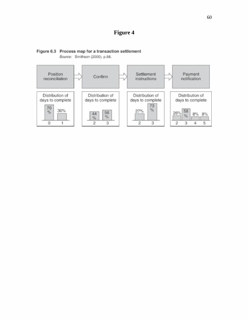
60

Figure 4

61

Figure 5, Panel A

Recession

Expansion

Low Volatility/ High Credit Quality

Assets

Time T = 1

B

62

Figure 5, Panel B

Recession

Expansion

High Volatility/ Low Credit Quality

Assets

Time T = 1

B

63

Table 1 Analysis of QIS Data: Basic Indicator Approach Based on 12% of Minimum Regulatory Capital

Median Mean Weighted Average

Std. Deviation

Weighted Aver. Std Deviation

Minimum 25th %-tile

75th %-tile

Maximum No. Of

Banks All

Banks 0.193 0.221 0.183 0.132 0.117 0.020 0.138 0.244 0.678 126

Large Banks

0.170 0.219 0.179 0.133 0.118 0.056 0.140 0.224 0.547 53

Small Banks

0.203 0.222 0.220 0.132 0.108 0.020 0.137 0.247 0.678 73

Source: BIS (September 2001), p. 27.

Table 2

Analysis of QIS Data: The Standardized Approach Based on 12% of Minimum Regulatory Capital

Lines

Of Business

Median Mean WeightedAverage

Std. Deviation

Weighted Aver. Std.

Deviation

Minimum 25th Percentile

75th Percentile

Ma

Corporate Finance

0.131 0.236 0.120 0.249 0.089 0.035 0.063 0.361 0

Trading & sales

0.171 0.241 0.202 0.183 0.129 0.023 0.123 0.391 0

Retail Banking

0.125 0.127 0.110 0.127 0.066 0.008 0.087 0.168 0

Commercial Banking

0.132 0.169 0.152 0.116 0.096 0.048 0.094 0.211 0

Payment & Settlement

0.208 0.203 0.185 0.128 0.068 0.003 0.100 0.248 0

Agency Services &

Custody

0.174

0.232

0.183

0.218

0.154

0.056

0.098

0.217 0

Retail Brokerage

0.113 0.149 0.161 0.073 0.066 0.050 0.097 0.199 0

Asset Management

0.133 0.185 0.152 0.167 0.141 0.033 0.079 0.210 0

Source: BIS (September 2001), p.29.

3

Table 3 Loss Event Type Classification: The Advanced Measurement Approach

Event Type Category

Definition Activity Examples

Internal Fraud Losses due to acts of a type in-tended to defraud, misappropriate property or

circumvent regulations, the law or company policy, excluding

diversity/discrimination events, which involves at least one internal party.

Unreported trans. (intentional); Unauthorized trans.; Mismarking of positions (intentional); credit fraud; worthless deposits; theft; extortion; embezzlement; misappropriation of

assets; forgery; check kiting; smuggling; impersonation; tax evasion (willful);

bribes; insider trading External Fraud Losses due to acts of a type intended to

defraud, misappropriate property or circumvent the law, by a third party.

Theft/robbery; forgery; check kiting; theft of information (with monetary loss);

hacking damage. Employment Practices and Workplace Safety

Losses arising from acts inconsistent with employment, health or safety laws

or agreements, from payment of personal injury claims, or from diversity/discrimination events.

Compensation, benefit, termination issues; organized labor activity; general liability; employee health & safety rules

events; workers compensation; all discrimination types.

Clients, Products, and Business Practices

Losses arising from an unintentional or negligent failure to meet a professional obligation to specific clients (including fiduciary and suitability requirements),

or from the nature or design of a product.

Fiduciary breaches; disclosure issues; breach of privacy; aggressive sales;

account churning; misuse of confidential information; lender liability; antitrust;

improper trade & market practices; market manipulation; insider trading (on

firm’s account); unlicensed activity; money laundering; product defects;

model errors; failure to investigate client per guidelines; exceeding client exposure limits; performance disputes for advisory

activities. Damage to Physical

Assets Losses arising from loss or damage to physical assets from natural disaster or

other events.

Natural disaster losses; human losses from external sources (terrorism,

vandalism). Business Disruption and System Failures

Losses arising from disruption of business or system failures.

Hardware; software; telecommunications; utility outage/disruptions.

Execution, Delivery and Process Management

Losses from failed transaction processing or process management,

from relations with trade counterparties and vendors.

Miscommunication; data entry, maintenance or loading error; missed deadline; system problem; accounting

error; delivery failure; collateral management failure; reference data

maintenance; failed mandatory reporting; inaccurate external report; client

disclaimers missing; legal documents missing; unapproved access given to

accounts; incorrect client records; negligent loss of client assets; non-client

counterparty misperformance; outsourcing vendor disputes.

Source: BIS (September2001), p. 21-23.

4

Table 4

The Relationship Between PD and Macroeconomic Conditions

Source: Altman (2002).

Year Default Rate Default Loss 3 Q 2001 6.92 % 5.29 %

2000 5.06 3.94 1999 4.15 3.21 1998 1.60 1.10 1997 1.25 0.65 1996 1.23 0.65 1995 1.90 1.24 1994 1.45 0.96 1993 1.11 0.56 1992 3.40 1.91 1991 10.27 7.16 1990 10.14 8.42

5

Table 5 The Relationship Between Recovery Rates

and Macroeconomic Conditions Altman with Brady (2001)

Year Senior Secured Senior Unsec. Subordinated All Securities 3Q2001 40.95 % 33.19 % 0 % 28.02%

2000 39.58 25.40 26.62 25.83 1999 26.90 42.54 13.88 31.14 1998 70.38 39.57 0 37.27 1997 74.90 70.94 60.00 53.89 1996 59.08 50.11 44.23 51.91 1995 44.64 50.50 20.00 41.77 1994 48.66 51.14 37.04 39.44 1993 55.75 33.38 28.38 38.83 1992 59.85 35.61 49.13 50.03 1991 44.12 55.84 24.30 40.67 1990 32.18 29.02 18.83 24.66

6

Table 6 Frye (2000b)

Paramter Values (1) (2) (3) (4) (5) Standard deviation

of recovery rate

0.32

0.32

0.32

0.25

0.25 PD 1.99% 2.00% 0.20% 2.00% 0.20%

Expected LGD 59.1%

30.7%

30.7%

30.7%

30.7%

Normal state PD 1.8%

1.7%

0.2%

1.7%

0.2%

Normal state LGD 55%

28%

27%

28%

28%

Depressed state PD 10.4%

14.8%

2.9%

14.8%

2.9%

Depressed state LGD

80%

52%

51%

47%

47%

Normal state Expected Loss

0.99%

0.48%

0.05%

0.48%

0.06%

Distressed state Expected Loss

8.32%

7.70%

1.48%

6.96%

1.36%

Note: For all model specifications, the systematic risk beta for assets (collateral) is 0.23 (0.17).

7

Table 7 Average Usage of Commitments to Lend

Asarnow and Marker (1995)

Credit Rating Prior to Default

Average Commitment Usage

Usage of normally unused commitment in the event

of default AAA 0.1 % 69 % AA 1.6 % 73 % A 4.6 % 71 %

BBB 20.0 % 65 % BB 46.8 % 52 % B 63.7 % 48 %

CCC 75.0 % 44 %

8

References

Acharya, V.V. and J.N. Carpenter, “Corporate Bond Valuation and Hedging with Stochastic Interest Rates and Endogenous Bankruptcy,” October 9, 2001, London Business School Working Paper. Acharya, V.V., J. Huang, M.G. Subramanhyam, and R.K. Sundaram, “When Does Strategic Debt Service Matter?” Working Paper, May 2, 2002. Allen, L., J. Boudoukh, A. Saunders, Value at Risk in Theory and Practice, Blackwell Publishing, 2003 forthcoming.

Allen, L., J. Jagtiani and Y. Landskroner, “Interest Rate Risk Subsidization in International Bank Capital Requirements,” Journal of Economics and Business, August 1996, 48, 251-267. Altman, E.I., Distressed Securities, Burr Ridge: Irwin Publishing, 1991 (reprinted by Beard Books, 1999). Altman, E.I., with P. Arman, “Defaults and Returns on High Yield Bonds: Analysis Through the First Quarter 2002,” Salomon Center Working Paper, April 2002. Altman, E.I., with B. Brady, “Explaining Aggregate Recovery Rates on Corporate Bond Defaults,” Salomon Center Working Paper, November 2001. Altman, E.I., A. Resti and A. Sironi, “Analyzing and Explaining Default Recovery Rates,” ISDA Resport, December 2001. Altman, E.I. and V. Kishore, “Almost Everything You Wanted to Know About Recoveries on Defaulted Bonds,” Financial Analysts Journal, 1996, vol. 52, no. 6, pp. 57-64 Altman, E.I., “Measuring Corporate Bond Mortality,” Journal of Finance, September 1989, vol. 44, no. 4, pp. 90-922. Anderson, R., S. Sundaresan, and P. Tychon, "Strategic Analysis of Contingent Claims." European Economic Review, April 1996, pp. 871-881. Anderson, R. and S. Sundaresan, “A Comparative Study of Structural Models of Corporate Bond Yields: An Exploratory Investigation,” Journal of Banking and Finance, vol. 24 (2000), pp. 255-269. Asarnow, E. and J. Marker, “Historical Performance of the US Corporate Loan Market 1988-1993,” Journal of Commercial Lending, vol. 10, no. 2, Spring 1995, pp. 13-32.

9

Ashcraft, A.B. and M. Campello, “Borrower’s Financial Constraints and the Transmission of Monetary Policy: Evidence from Financial Conglomerates,” Federal Reserve Bank of New York Staff Reports, No. 153, August 2002. Ayuso, J., D. Perez and J. Saurina, “Are Capital Buffers Procyclical?” Banco de Espana working paper, April 2002. Baker, M. and J. Wurgler, “The Equity Share in New Issues and Aggregate Stock Returns,” Journal of Finance, October 2000, vol. 55, no. 5, pp. 2219-2258. Bakshi, G., D. Madan, and F. Zhang, “Investigating the Sources of Default Risk: Lessons from Empirically Evaluating Credit Risk Models,” University of Maryland working paper, February 28, 2001. Bali, T., “The Generalized Extreme Value Distribution: Implications for the Value at Risk,” Working Paper, Baruch College Zicklin School of Business, February 2001. Bangia, A., F.X. Diebold, T. Schuermann, “Ratings Migration and the Business Cycle, With Applications to Credit Portfolio Stress Testing.” Wharton Financial Institutions Center, Working Paper 26, April 2000. Bank for International Settlements, Standardized Model for Market Risk. Basle, Switzerland: Bank for International Settlements, 1996. Bank for International Settlements, “Marrying the Macro- and Microprudential Dimensions of Financial Stability,” BIS Papers No. 1, March 2001. Bank for International Settlements, “Working Paper on the Regulatory Treatment of Operational Risk,” September 2001. Bank for International Settlements, “Supervisory Guidance on Dealing with Weak Banks: Report of the Task Force on Dealing with Weak Banks,” March 2002. Barnhill, T.M., Jr., and W. F. Maxwell, “Modeling Correlated Interest Rate, Spread Risk, and Credit Risk for Fixed Income Portfolios.” Journal of Banking and Finance, February 2002, vol. 26 2/3, pp. 347-374. Bekaert, G., and C.R. Harvey, “Time-Varying World Market Integration,” Journal of Finance, 50, 2, June 1995, pp. 403-444. Bekaert, G. C.R. Harvey, R.L. Lumsdaine, “Dating the Integration of World Equity Markets,” Journal of Financial Economics, 65, 2002, pp. 203-247. Belkin, B., S. Suchower, and L.R. Forest, “The Effect of Systematic Credit Risk on Loan Portfolio Value-at-Risk and Loan Pricing,” CreditMetrics Monitor, First Quarter 1998, pp. 17-28.

10

Berger, A.N. and G.F. Udell, “Institutional Memory, the Business Cycle and Bank Lending Behavior,” Presented at the Conference on Changes in Risk through Time: Measurement and Policy Options, March 6, 2002. Berger, A.N. and G.F. Udell, “Did Risk-Based Capital Allocate Bank Credit and Cause a ‘Credit Crunch’ in the United States?” Journal of Money, Credit and Banking, vol. 26, 1994, pp. 585-628. Bernanke, B.S. and C.S. Lown, “The Credit Cturnch,” Brookings Papers on Economic Activity, No. 2, 1991, pp. 205-248. Bhansali, V. and M.B. Wise, “Forecasting Portfolio Risk in Normal and Stressed Markets,” Journal of Risk, Fall 2001, vol. 4, no. 1, pp. 91-106. Bongini, P. L. Laeven, G. Majnoni, “How Good is the Market at Assessing Bank Fragility? A Horse Race Between Different Indicators,” Journal of Banking and Finance, vol. 26, 2002, pp. 1011-1028. Borio, C., C. Furfine, and P. Lowe, “Procyclicality of the Financial System and Financial Stability: Issues and Policy Options,” BIS working paper, February 2001. Borio, C. and P. Lowe, “Asset Prices, Financial and Monetary Stability: Exploring the Nexus,” BIS working paper, January 7, 2002. Calomiris, C.W. and R.J. Herring, “The Regulation of Operational Risk in Investment Management Companies,” Investment Company Institute Perspective, vol. 8, no. 2, September 2002, p. 2-19. Carey, M., "Credit Risk in Private Debt Portfolios." Journal of Finance, August 1998, pp. 1363-1387. Cavallo, M., and G. Majnoni, “Do Banks Provision for Bad Loans in Good Times? Empirical Evidence and Policy Implications.” World Bank, Working Paper 2691, June 2001. Chang, G. and S.M. Sundaresan, “Asset Prices and Default-Free Term Structure in an Equilibrium Model of Default.” Columbia University Working Paper, October 1999. Chiuri, M.C., G. Ferri, and G. Majnoni, “The Macroeconomic Impact of Bank Capital Requirements in Emerging Economies: Past Evidence to Assess the Future,” Journal of Banking and Finance, vol. 26, 2002, pp. 881-904. Collin-Dufresne, P. and B. Solnik, “On the Term Structure of Default Premia in the Swap and LIBOR Markets.” Journal of Finance, June 2001, pp. 1095-1115.

11

Collin-Dufresne, P. and Goldstein, R., “Do Credit Spreads Reflect Stationary Leverage Ratios?” Journal of Finance, October 2001, vol. LVI, no. 5, pp. 1929-1957. Collin-Dufresne, P., Goldstein, R. and J.S. Martin, “The Determinants of Credit Spreads Changes” Journal of Finance, December 2001, vol. LVI, no. 6, pp. 2177-2207 Crouhy, M., D. Galai, and R. Mark, “Prototype Risk Rating System.” Journal of Banking and Finance, January 2001, pp. 47-95. Crouhy, M., D. Galai, and R. Mark, "A Comparative Analysis of Current Credit Risk Models." Journal of Banking and Finance, January 2000, pp. 57-117. Cummins, J.D., N. Doherty and A. Lo, “Can Insurers Pay for the ‘Big one?’ Measuring the Capacity of the Insurance Market to Respond to Catastrophic Losses,” Journal of Banking and Finance, 2002, 26, pp. 557-583. Dalianes, P.C. “Credit Risk Pricing: Summary and Current Methodology,” Quantitative Models in Finance, 1999. Das, S.R., L. Freed, G. Geng, N. Kapadia, “Correlated Default Risk,” September 14, 2001 Working Paper, Santa Clara University. Das, S.R., G. Fong, G. Geng. “The Impact of Correlated Default Risk on Credit Portfolios,” September 14, 2001 Working Paper, Santa Clara University. De Nicolo, G. and M.L. Kwast, “Systemic Risk and Financial Consolidation: Are They Related?” Journal of Banking and Finance, vol. 26, 2002, pp. 861-880. Duffee, G.R., "Estimating the Price of Default Risk." The Review of Financial Studies, Spring 1999, pp. 197-226 Duffie, D. and K.J. Singleton, “Modeling the Term Structures of Defaultable Bonds,” Review of Financial Studies, 1999, vol. 12, pp. 687-720. Duffie, D., and K.J. Singleton, "Simulating Correlated Defaults." Paper presented at the Bank of England Conference on Credit Risk Modeling and Regulatory Implications, London, September 21-22,1998. Duffie, D. and Lando, D., “Term Structures of Credit Spreads with Incomplete Accounting Information,” Econometrica, vol. 69, 2001, pp. 663-664. Elsinger, H., A. Lehar, M. Summer, “The Risk of Interbank Credits: A New Approach to the Assessment of Systemic Risk,” February 2002, Austrian Central Bank Working Paper.

12

Erlenmaier, U. and H. Gersbach, “Default Probabilities and Default Correlations,” February 2001 Working Paper, University of Heidelberg, February 2001. Estrella, A., “The Cyclical Behavior of Optimal Bank Capital,” Federal Reserve Bank of New York Working Paper, December 2001. Falkenheim, M. and A. Powell, “The Use of Credit Bureau Information in the Estimation of Appropriate Capital and Provisioning Requirements.” Central Bank of Argentina, Working Paper, 2001. Fama, E., “Term Premiums and Default Premiums in Money Markets,” Journal of Financial Economics, 1986, vol. 17, np. 1, pp. 175-196. Ferri, G., L.G. Liu, and G. Majnoni, “The Role of Rating Agency Assessments in Less Developed Countries: Impact of the Proposed Basel Guidelines.” Journal of Banking and Finance , January 2001, pp. 115-148. Finger, C.C., “Conditional Approaches for CreditMetrics Portfolio Distributions.” Riskmetrics Monitor, April 1999. Fridson, M., C. Garman, and S. Wu, “Real Interst Rates and the Default Rates on High-Yield Bonds,” Journal of Fixed Income, September 1997, pp. 27-34. Fruhwirth, M. and L. Sogner, “The Jarrow/Turnbull Default Risk Model: Evidence from the German Market,” Vienna University Working Paper, October 8, 2001. Frye, J., “Collateral Damage,” Risk, April 2000a, 91-94. Frye, J., “Depressing Recoveries,” Risk, November 2000b, 108-111. Gersbach, H. and U. Wehrspohn, “Lean IRB Approaches and Transition Design: The Basel II Proposal,” University of Heidlberg working paper, October 2001. Geyer, A., S. Kossmeier, and S. Pichler, “Empirical Analysis of European Government Yield Spreads,” Vienna University of Technology Working Paper, March 2001. Giesecke, K., “Compensator-Based Simulation of Correlated Defaults,” April 30, 2002, Humboldt-Universitat zu Berlin Working Paper. Goldberg, L., J. Kambhu, J.M. Mahoney, L. Radecki, A. Sarkar, “Securities Trading and Settlement in Europe: Issues and Outlook,” Journal of Financial Transformation, the Capco Institute, vol. 5, 2002, pp. 83-89.

13

Goodhart, C., “Price Stability and Financial Fragility,” in K. Sawamoto, Z. Nakjima and H. Taguchi, eds., Financial Stability in a Changing Environment, St. Martin’s Press, 1995. Gordy, M., “A Risk Factor Model Foundation for Ratings-Based Bank Captial Rules,” Board of Governors of the Federal Reserve System Working Paper, February 2001. Gross, D.B. and N.S. Souleles, “An Empirical Analysis of Personal Bankruptcy and Delinquency,” The Review of Financial Studies, Spring 2002, vol. 15, no. 1, pp. 319-347. Gupton, G.M., D. Gates and L.V. Carty, “Bank-Loan Loss Given Default,” Moody’s Investors Service, Global Credit Research, November 2000. Hancock, D. and J.A. Wilcox, “Was There a ‘Capital Crunch’ in Banking? The Effects on Real Estate Lending of Business Conditions and Capital Shortfalls,” Journal of Housing Economics, vol. 3, no. 1, December 1993, pp. 75-105. Hancock, D. and J.A. Wilcox, “Bank Balance Sheet Shocks: Are There Dynamic Effects on Bank Capital and Lending?” Journal of Banking and Finance, vol. 19, 1995, pp. 661-677. Harr, T., “Bad Loans and Liquidation: The Case of Japan,” University of Copenhagen Working Paper, November 30, 2001. Hillegeist, S.A., D.P. Cram, E.K. Keating, K.G. Lundstedt, “Assessing the Probability of Bankruptcy,” Working Paper, April 2002. Hofmann, B., “The Determinants of Private Sector Credit in Industrialised Countries: Do Property Prices Matter,” Bank for International Settlements Monetary and Economic Department working paper, December 2001. Hoggarth, G., R. Reis, V. Saporta, “Costs of Banking System Instability: Some Empirical Evidence,” Journal of Banking and Finance, vol. 26, 2002, pp. 825-855. Houweling, P., and T. Vorst, “An Empirical Comparison of Default Swap Pricing Models,” Erasmus University working paper, December 21, 2001. Hull, J. and A. White, “The Impact of Default Risk on the Prices of Options and Other Derivative Securities,” Journal of Banking and Finance, 1995, vol. 19, pp. 299-322. Instefjord, N., P. Jackson and W. Perraudin, “Securities Fraud and Irregularities,” ,” in Operational Risk and Financial Institutions, Arthur Andersen Risk Books, 1998, pp. 147-158.

14

Jackson, P., W. Perraudin, and V. Saporta, “Setting Minimum Capital for Internationally Active Banks.” Paper presented at the Bank of England Conference on Banks and Systemic Risk, London, May 23-25, 2001. Jarrow, R.A., “Default Parameter Estimation Using Market Prices.” Financial Analysts Journal, September/October 2001, pp. 75-92. Jarrow, R.A. and F. Yu, “Counterparty Risk and the Pricing of Defaultable Securities,” Journal of Finance, October 2001, 1765-1799. Jarrow, R.A., Van Deventer, D.R., X. Wang, “A Robust Test of Merton’s Structural Model for Credit Risk,” Kamakura Corporation working paper, April 21, 2002. Jokivuolle, E. and S. Peura, “Incorporating Collateral Value Uncertainty in Loss-Given-Default Estimates and Loan-to-Value Ratios,” Bank of Finland Discussion Papers 2/2000. Jordan, J., J. Peek, and E. Rosengren, “Credit Risk Modeling and the Cyclicality of Capital,” BIS conference, March 6, 2002. Kim, J., “Conditioning the Transition Matrix.” Credit Risk, October 1999, pp. 37-40. Kim, I.J., K. Ramaswamy, S. Sundaresan, “Does Default Risk in Coupons Affect the Valuation of Corporate Bonds? A Contingent Claims Model,” Financial Management, 1993, vol. 22, no. 3, pp. 117-131. Lando, D., “On Cox Processes and Credit Risky Securities,” Review of Derivatives Research, 1998, vol. 2, pp. 99-120. Leland, H., "Corporate Debt Value, Bond Covenants and Optimal Capital Structure." Journal of Finance, September 1994, pp. 1213-1252. Levy, H. and M. Sarnat, “International Diversification of Investment Portfolios,” American Economic Review, 60, 1970, pp. 668-692. Longin, F., and B. Solnik, “Extreme Correlation of International Equity Markets,” Journal of Finance, April 2001, vol. LVI, no. 2, pp. 649-676. Longstaff, F.A., and E.F. Schwartz, "A Simple Approach to Valuing Risky Fixed and Floating Rate Debt." Journal of Finance, July 1995, pp.789-819. Lopez, J.A., “The Empirical Relationship Between Average Asset Correlation, Firm Probability of Default and Asset Size,” Federal Reserve Bank of San Francisco working paper, April 23, 2002.

15

Lowe, P., “Credit Risk Measurement and Procyclicality,” BIS Working Papers, No. 116, September 2002. Lown, C.S., and D.P. Morgan, “The Credit Cycle and the Business Cycle: New Findings Using the Survey of Senior Loan Officers.” Federal Reserve Bank of New York, Working Paper, June 25, 2001. Lown, C.S. and S. Peristiani, “The Behavior of Consumer Loan Rates During the 1990 Credit Slowdown,” Journal of Banking and Finance, vol. 20, 1996, pp. 1673-1694. Lucas, D., “Default Correlation and Credit Analysis,” Journal of Fixed Income, March 1995, pp. 76-87. Maclachlan, I., “Recent Advances in Credit Risk Management.” Ninth Melbourne Money and Finance Conference, June 19, 1999. Madan, D.B. and H. Unal, “A Two-Factor Hazard-Rate Model for Pricing Risky Debt and the Tern Structure of Credit Spreads.” Journal of Financial and Quantitative Analysis, March 2000, pp.43-65. Marshall, C. Measuring and Managing Operational Risk in Financial Institutions, John Wiley & Sons (Asia) Pte Ltd, Singapore: 2001. McNeil, A.J., “Extreme Value Theory for Risk Managers,” Working Paper, Department of Mathematics, Swiss Federal Technical University, Zurich, May 1999. Mei, J. and A. Saunders, “Have US Financial Institutions’ Real Estate Investments Exhibited “Trend Chasing” Behavior?” The Review of Economics and Statistics, 1997, pp. 248-258. Mella-Barral, P., and W. Perraudin, "Strategic Debt Service."' Journal of Finance, June 1997, pp. 531-556. Monfort, B. and C. Mulder, “Using Credit Ratings for Capital Requirements on Lending to Emerging Market Economies - Possible Impact of a New Basel Accord .“ International Monetary Fund, Working Paper WP/00/69, 2000. Mueller, C., “A Simple Multi-Factor Model of Corporate Bond Prices.” Doctoral Dissertation University of Wisconsin-Madison, October 29, 2000. Neftchi, S.N., “Value at Risk Calculations, Extreme Events, and Tail Estimation,” Journal of Derivatives 7, no. 3, Spring 2000, pp. 23-38. Nickell, P., W. Perraudin, and S. Varotto, “Stability of Rating Transitions.” Journal of Banking and Finance, vol. 24 no. 1/2, 2000, pp. 203-228.

16

Peek, J. and E.S. Rosengren, “The Capital Crunch: Neither a Borrower Nor a Lender Be,” Journal of Money, Credit and Banking, vol. 27, no. 3, August 1995, pp. 625-638. Pulvino, T.C., “Do Asset Fire Sales Exist? An Empirical Investigation of Commercial Aircraft Transactions,” Journal of Finance, June 1998, vol. LIII, no. 3, pp. 939-978. Purhonen, M., “New Evidence of IRB Volatility,” Risk, March 2002, pp. S21-S25. Pykhtin, M. and A. Dev, “Analytical Approach to Credit Risk Modeling,” Risk, March 2002, pp. S26-S32. Reisen, H., “Revisions to the Basel Accord and Sovereign Ratings.” in R. Hausmann and U. Hiemenz (eds.), Global Finance From a Latin American Viewpoint, IDB/OECD Development Centre, 2000. Saunders, A., “Comments on ‘The Macroeconomic Impact of Bank Capital Requirements in Emerging Economies: Past Evidence to Assess the Future,” Journal of Banking and Finance, vol. 26, 2002, pp. 905-907. Saunders, A. and L. Allen, Credit Risk Measurement: New Approaches to Value at Risk and Other Paradigms, New York: John Wiley and Sons, 2002. Schwebach. R.G., J.P. Olienyk, J.K. Zumwalt, “The Impact of Financial Crises on International Diversification,” Global Finance Journal, 13 June 2002, pp. 147-161. Solnik, B., Boucrelle, C. and Le Fur, Y., “International Market Correlation and Volatility,” Financial Analysts Journal, 52, 1996, pp. 17-34. Unal, H., D. Madan, and L. Guntay, “A Simple Approach to Estimate Recovery Rates with APR Violation from Debt Spreads.” Wharton Financial Institutions Center, Working Paper 7, February 2001, Journal of Banking and Finance, forthcoming. Varotto, S., “Credit Risk Diversification,” University of Reading Working Paper, 2002. Westphalen, M., “Valuation of Sovereign Debt with Strategic Defaulting and Rescheduling,” University of Lausanne Working Paper, February 26, 2002. Wilson, T., "Credit Risk Modeling: A New Approach." New York: McKinsey Inc., 1997a (mimeo). Wilson, T., "Portfolio Credit Risk (Parts I and II)." Risk Magazine, September and October, 1997b. Zhou, C., “An Analysis of Default Correlations and Multiple Defaults.” The Review of Financial Studies, Summer 2001, pp. 555-576.