Incorporating Liquidity Risk in Value ... -...

Incorporating Liquidity Risk in Value-at-Risk

Based on Liquidity Adjusted Returns∗

Lei Wu†

Research Institute of Economics and Management,

Southwestern University of Economics and Finance

Abstract

In this paper, based on Acharya and Pedersen’s [Journal of Financial Eco-

nomics (2006)] overlapping generation model, we show that liquidity risk could

influence the market risk forecasting through at least two ways. Then we argue

that traditional liquidity adjusted VaR measure, the simply adding of the two

risk measure, would underestimate the risk. Hence another approach, by mod-

eling the liquidity adjusted returns (LAr) directly, was employed to incorporate

liquidity risk in VaR measure in this study. Under such an approach, China’s

stock market is specifically studied. We estimate the one-day-ahead “standard”

VaR and liquidity adjusted VaR by forming a skewed Student’s t AR-GJR

model to capture the asymmetric effect, non-normality and excess skewness of

return, illiquidity and LAr. The empirical results support our theoretical ar-

guments very well. We find that for the most illiquidity portfolio, liquidity risk

represents more than 22% of total risk. We also find that simply adding of the

two risk measure would underestimate the risk. The accuracy testing show that

our approach is more accurate than the method of simply adding.

JEL Classification Codes: G11; G12; G18

Keywords: Value-at-Risk(VaR); Liquidity risk; Liquidity adjusted returns; Skewed

Student’s t; GJR model

∗This research was supported by a grant from the “Project 211 (Phase III )” of the Southwestern

University of Finance and Economics.†Research Institute of Economics and Management, Southwestern University of Economics and Fi-

nance, 55 Guanghuacunjie, Chengdu, Sichuan, 610074, China. Email address: [email protected]

3VaR�.¥i\6Ä5ºxµÄu6Ä5

N�ÂÃÇ��{∗

É [†

ÜHã²�Æ²L�+nïÄ�

ÁÁÁ ��

�©3Acharya and Pedersen (2006)�ªVU��.Ä:þ§y²6Ä5

ºx�±ÏL��ü«�ªK�½|ºx"âd§·�?�ÚØy§ÏLò½

|ºxÚ6Ä5ºx{ü�\ ¼�6Ä5N��VaR��{¬$�ºx"Ï

d§·�3ù�©Ù¥��é6Ä5N�ÂÃÇï�§l ýÿ6Ä5N�

�VaR§¿^ù«�{ïÄ¥I�¦½|"��ÂÃÇS�!�6Ä5¤

�S�Ú6Ä5N�ÂÃÇS�¥��é¡5!��5Ú 5A:§·�ï

á�� t©Ù�AR-GJR�.ýÿ/IO0VaRÚ6Ä5N��VaR"¢y

(JéÐ�|±·�nØ�.�ýÿ"·�uyé6Ä5��]�|Ü

ó§6Ä5ºx�±Ó�oºx�22%"·��uy{ü�\��{(¢$�

ºx"ÚOu��(Jy¢·��{'{ü�\��{��°("

JEL ©©©aaaÒÒÒ: G11; G12; G18

'''��ccc: 3xd�(VaR)¶6Ä5ºx¶6Ä5N�ÂÃÇ¶ t©Ù¶GJR�.

∗�©��ÜHã²�Æ/211ó§0nÏï��8]Ï"†oA�¤Ñ½1u~�55ÒÜHã²�Æ²L�+nïÄ�§610074"

>fe�µ[email protected]

1 Introduction

Value-at-Risk (VaR) has been widely used in risk measurement by many financial

institutions. But a fundamental assumption underlying the traditional VaR models

is that assets can be traded in a liquid market. In reality, however, the capital

market is not as liquid as we expect. Investors face not only the market risk but also

the liquidity risk. Moreover, the bankruptcy of Long-Term Capital Management

(LTCM) tell us that the illiquidity “is a big source of risk to an investor”1. Hence,

it is necessary to incorporate liquidity risk in the VaR measure.

Few studies has focused on this issue2. For instance, Bangia et al. (1999) esti-

mate the worst increase the bid-ask spread may suffer. They add it to the “standard”

VaR and then obtain a liquidity adjusted VaR measure. More recently, Angelidis

and Benos (2006) estimate a trade volume dependent model based on the com-

ponents of the bid-ask spread and then incorporate a parametric liquidity risk in

“standard” VaR measure. However, the most of these researches modeling the mar-

ket risk and liquidity risk separately, and then add the two risk measure—value at

market risk and value at liquidity risk. But recent development in asset pricing and

market microstructure theories point out that liquidity risk should be priced (see,

for example, Amihud and Mendelson, 1986; Holmstrom and Tirole, 2001; Acharya

and Pedersen, 2006). Most empirical evidences also show that illiquidity securities

should have higher expected returns (see, for instance, Brennan et al., 1998; Ami-

hud, 2002; Pastor and Stambaugh, 2003). Hence, it maybe inaccurate in calculating

liquidity adjusted VaR if we omit the relation between liquidity risk and market risk.

In this paper, based on Acharya and Pedersen’s (2006) overlapping generation

(OLG) model, we show that liquidity risk can influence the market risk forecasting

through two ways. Then the accuracy of simply adding of the two risk measure would

also be influenced through two ways: 1) First, as been shown in existed literatures,

returns are low when illiquidity increases. Therefore, the value at market risk would

increase and the simply adding would underestimate the risk. 2) Second, we show

that the volatility of returns would be amplified if the volatility of illiquidity risk

is large. Then the value at market risk would also increase and the simply adding

would underestimate the risk, too. At a word, just add the two risk measure would

underestimate the liquidity adjusted VaR.

1The Economist, September 23, 1999.2See the section 1 of Angelidis and Benos(2006) for a nice survey.

1

Hence, we employ another method to incorporate liquidity risk in VaR measure.

We modeling the liquidity adjusted returns (LAr) directly, where the LAr is equal to

returns minus illiquidity cost. Since LAr itself considering the market risk and the

liquidity risk simultaneously, this approach can avoid the underestimate problem in

the simply adding of value at market risk and value at liquidity risk. Moreover, LAr

satisfies Artzner et al ’s (1999) “future value” viewpoint because it is the actually

value of one unit of assets when investors need to liquidate the assets.

Under such an approach, China’s stock market is specifically studied, a market

considered as a very important emerging market. We form a skewed Student’s t AR-

GJR model to estimate the one-day-ahead “standard” VaR and liquidity adjusted

VaR. We find that for the most illiquidity portfolio, liquidity risk represents more

than 22% of total risk. We also find that simply adding of the two risk measure would

underestimate the risk. The accuracy testing based on Kupiec’s (1995) statistic show

that our approach is more accurate than the method of simply adding.

Three main contributions are belong to this paper. Firstly, we propose a more

accurate approach to modeling liquidity adjusted VaR. Secondly, this study adds

to the evidence on the importance of liquidity risk in VaR measure. Lastly, there

are rarely studies considering China’s stock market about such issue in international

journals. But China has became the most important emerging market and its stock

market has been opened to international investors. Hence we need more researches,

such as this paper, to study the characteristic of the risk in China’s stock market.

The remainder of this paper is organized as follows. In Section 2, we will show

the inaccuracy of the method of simply adding. Section 3 presents the data and

econometric model. In Section 4, we will report the empirical results. Section 5

concludes the paper.

2 Theoretic framework

2.1 market risk and liquidity risk

In this subsection, we would find the relation between liquidity risk and market

risk by simplifying Acharya and Pedersen’s (2006) OLG model. The model assumes

generation t, which is born at time t ∈ {...,−2,−1, 0,−1, 2, ...} and lives in period

t and t + 1, consists of N agents. Agent n of generation t only has an endowment

ent in period t. We assume he trades in period t and t + 1 and maximizes his expect

utility function −Et exp (−γxt+1), where γ is his constant absolute risk aversion and

2

xt+1 is his consumption at time t + 1. Since there is no other source of income, the

utility function is equal to −Et exp (−γWt+1), where Wt+1 is the derived wealth by

trading.

Suppose there are two kinds of asset, the risky asset with total of S shares and

the riskfree asset. At time t, the risky asset has a share price of Pt, and has a per-

share illiquidity cost of Ct. Hence, agents can buy the risky asset at Pt but must sell

it at Pt − Ct. Pt and Ct are both random variables. Uncertainty about Pt is what

generates the market risk in this model. Similarly, uncertainty about Ct generates

the liquidity risk. Moreover, the illiquidity cost Ct is assumed to be autoregressive

process of order one, that is

Ct = C + ρC(Ct−1 − C) + ηt, (1)

where C ∈ R+, ρC ∈ [0, 1], and ηt is an independent identically distributed process

with zero mean and variance V ar(ηt) = ΣC .

We assume the gross return of the riskfree asset is Rf (Rf > 1). For the the risky

asset’s (net) return

rt =Pt

Pt−1− 1 (2)

and its relative illiquidity cost

ct =Ct

Pt−1, (3)

we can obtain two implications3:

Proposition 1. 4 Returns are low when illiquidity increases,

Covt(ct+1, rt+1) < 0. (4)

There are lots of empirical evidences consistent with this proposition both in

developed markets and emerging markets. For examples, Amihud (2002) finds a

negative relation between the return on size portfolios traded in NYSE and their

corresponding unexpected illiquidity; Bekaert et al.(2007) finds a negative relation

between the returns and illiquidity for emerging markets.

Proposition 2. The conditional variance of returns increases with the conditional

variance of illiquidity,

∂V art(rt+1)

∂V art(Ct+1)> 0. (5)

3See appendix for proves.4This proposition is similar to Proposition 3 in Acharya and Pedersen(2006).

3

The relation between the second moments of returns and illiquidity always be

omitted in literatures. However, it is important to consider variance in risk mea-

surement. Practically, we would find that both kinds of relation could influence the

accuracy of the simply adding of the two risk measure.

2.2 Incorporating liquidity risk in VaR

Value-at-Risk (VaR) is defined as the worst outcome that is expected to occur

over a predetermined period and at a given confidence level (say 1 − α). The tra-

ditional VaR measure, VaR(r), focuses on the market risk but doesn’t consider the

liquidity risk. In fact, we should compute

VaR(r + (−c)) (6)

if we want to incorporate liquidity risk in VaR. Using −c here because c is defined as

illiquidity in the assumption. In most of literatures, the market risk and the liquidity

risk were modeled separately. The liquidity adjusted VaR was calculated by simply

adding of the two risk measure, that is

VaR(r + (−c)) = VaR(r) + VaR(−c). (7)

But as shown above, there exit at least two kinds of relation between the liquidity

risk and the market risk. We now analyze the impact of the two kinds of relationship

on the above method. Without loss generality, we focus on the one-step-ahead VaR

computed in time t

VaRt(rt+1 + (−ct+1)) = VaRt(rt+1) + VaRt(−ct+1). (8)

Firstly, according to proposition 1, we have Covt(ct+1, rt+1) < 0. Since VaRt(−ct+1)

refers to the worst increase the illiquidity may suffer, the probability that rt+1 would

be low will increase when we consider the liquidity risk. Therefore, if we isolate the

calculating of VaRt(rt+1) from the calculating of VaRt(−ct+1), we would underes-

timate the risk. Contrarily, since VaRt(rt+1) is defined as the worst outcome the

return may occur, the probability that ct+1 would be high will increase when we con-

sider the VaR measure of the market risk. Hence, we would also underestimate the

risk if we isolate the calculating of VaRt(−ct+1) from the calculating of VaRt(rt+1).

Secondly, according to proposition 2, we have ∂V art(rt+1)∂V art(Ct+1) > 0. We know that

the one-step-ahead VaR measure of the market risk is computed as

VaRt(rt+1) = µrt+1 + zr

ασrt+1, (9)

4

where µrt+1 is the conditional mean of the asset’s return and σr

t+1 the conditional

standard variance of the return. zrα is the left quantile at α for the empirical dis-

tribution of the return. Since σrt+1 increases with the conditional standard variance

of the illiquidity risk, VaRt(rt+1) would be high (in absolute value) when we con-

sider the liquidity risk5. Hence, we would underestimate the risk if we isolate the

calculating of VaRt(rt+1).

To sum up, the simply adding of the two risk measure would underestimate the

liquidity adjusted VaR. We suggest that it is more accurate to model the liquidity

adjusted returns (LAr) directly, where LAr is equal to returns minus illiquidity cost.

Since LAr itself considering the market risk and the liquidity risk simultaneously,

this approach can avoid the underestimate problem in the simply adding of value

at market risk and value at liquidity risk. Moreover, LAr satisfies Artzner’s (1999)

“future value” viewpoint because it is the actually value of one unit of assets when

investors need to liquidate the assets. Then we should calculate VaR(LAr) in this

paper. To highlight the importance of the liquidity risk, we define and compute the

relative liquidity risk proportion

ℓ =VaR(LAr) − VaR(r)

VaR(LAr). (10)

3 Data and econometric models

China’s stock market is specifically studied in this paper, transaction data cover

the period from 2 January 2001 to 31 December 2008. Before describing our data

set in detail, we first introduce the illiquidity measure used in this study.

3.1 The illiquidity measure

The concept of (il)liquidity is elusive. Literatures about liquidity focus on one

kind or several kinds of liquidity proxy because it is not observed directly. For

examples, Amihud and Mendelson (1986) use the bid-ask spread relating to trading

cost; Pastor and Stambaugh (2003) form a monthly liquidity measure by regressing

individual stock’s return minus the market return on the lagged individual stock’s

return and the lagged signed dollar trading volume using daily data; Amihud (2002)

defined illiquidity as the average ratio of the daily absolute return to the dollar

trading volume on that day; Bekaert et al.(2007) construct the proportion of zero

5If we don’t consider the liquidity risk, it is same to assume the mean and variance of illiquidity are

both equal to zero.

5

daily returns observed over the relevant month for emerging market as liquidity

measure. In the literatures of liquidity adjusted VaR, bid-ask spread is a widely used

illiquidity measure. For instance, Bangia et al. (1999) classify illiquidity into the

exogenous illiquidity and the endogeneous illiquidity and employ the bid-ask spread

to represent the former. Based on the components of the bid-ask spread, Angelidis

and Benos (2006) use order-based proxies of liquidity. In emerging markets, however,

detailed transaction data of the bid-ask spreads are not widely available, especially

for long time series. Hence, we employ Amihud (2002)’s illiquidity measure using

only daily data. Particularly, the illiquidity of stock i in day t is

ILLIQit =

|rit|

V it

, (11)

where rit and V i

t are the return and yuan6 volume (in ten millions) for stock i on

day t, respectively.

This illiquidity measure has been widely used in empirical studies, and has been

shown to be a valid instrument for the illiquidity. ILLIQ is positively related to

price impact to capture the price reaction to trading volume (Liu, 2006). Hasbrouck

(2002) finds that the Spearman (Pearson) correlation between ILLIQ and a measure

of Kyle’s (1985) lambda is 0.737 (0.473) in the USA. Yuan volume in ten millions

means that we assume the investor’s position is ten millions yuan, and the illiquidity

cost is positively related to trade demands. Therefore, ILLIQ captures both the

exogenous illiquidity and the endogeneous illiquidity in Bangia et al. (1999).

ILLIQ, in terms of return impact, can be viewed as the cost of 10 millions

yuan trade. But China’s stock market experiences a rapidly growth in the sample

period— the market capitalizations of the market portfolio increase by almost 832

percent from January 2001 to December 20087. Obviously, 10 millions yuan trade

was more substantial in January 2001 than December 2008, so ILLIQ tend to be

smaller in magnitude later in the period. Hence follow Pastor and Stambaugh (2003),

we construct the scaled series (mh/m1)ILLIQit, where mh is the total value of the

market at the end of month h corresponding to day t, and m1 is the total value of

the market at the end of January 2001. Finally, the illiquidity measure for stock i

at day t we used is

cit = min{mh

m1ILLIQi

t, 10.00}. (12)

6Yuan is the units of Renminbi (RMB, the Chinese currency).7The total value of the market at the end of January 2001 and at the end of December 2008 are

1567768 and 14602379 millions yuan, respectively.

6

3.2 Data

China has two stock exchanges, the Shanghai stock exchange (SHSE) and the

Shenzhen stock exchange (SZSE). The two were both inaugurated in the early 1990s,

and the SZSE is relatively smaller. Chinese company can raise funds through an A

or B share listing on one of the two exchanges. The A shares are held by Chinese

citizens and purchased in RMB, while B shares are held by foreign parties and

denominated in U.S. dollars. Since only a few firms offer B shares and the B shares

always experience a light trading, we focus on the A shares only. In the remainder of

this paper, the A shares market of the SHSE and the A shares market of the SZSE

are, respectively, abbreviated to SHSE-A and SZSE-A.

The data used in this paper for the two stock exchanges are from the CSMAR

China Stock Market Trading Database, which imitates CRSP and be widely used by

Chinese academe and financial companies. For each year t (2001-2008), we allocate

all the firms listed in the SHSE-A and the SZSE-A into five size-portfolios (from

small to big: S1, S2, S3, S4 and S5) based on their market capitalization at the

end of December of year t − 1. For all stocks, the days with no trading have been

eliminated from the sample. Value-weight daily returns (in percent) and illiquidity

costs (in percent) on the portfolios are calculated from the first trading day to the last

trading day of year t. Particularly, for each portfolio p (p ∈ {S1, S2, S3, S4, S5}),its return at day t is

rpt =

∑

i in p

witr

it, (13)

and the illiquidity cost at day t is

cpt =

∑

i in p

witc

it, (14)

where wit are value-based weights. Suppose month h is corresponding to the day t,

then we form the weights based on the market value for firm i at the end of month

h − 1. Similarly, we compute the LAr (in percent) of portfolio p at day t, as

LArpt =

∑

i in p

witLAri

t

=∑

i in p

wit(r

it − ci

t). (15)

The number of valid observation days in the sample for each portfolio is 1932.

We plot rpt , cp

t and LArpt in figure 1, figure 2 and figure 3, respectively. These

7

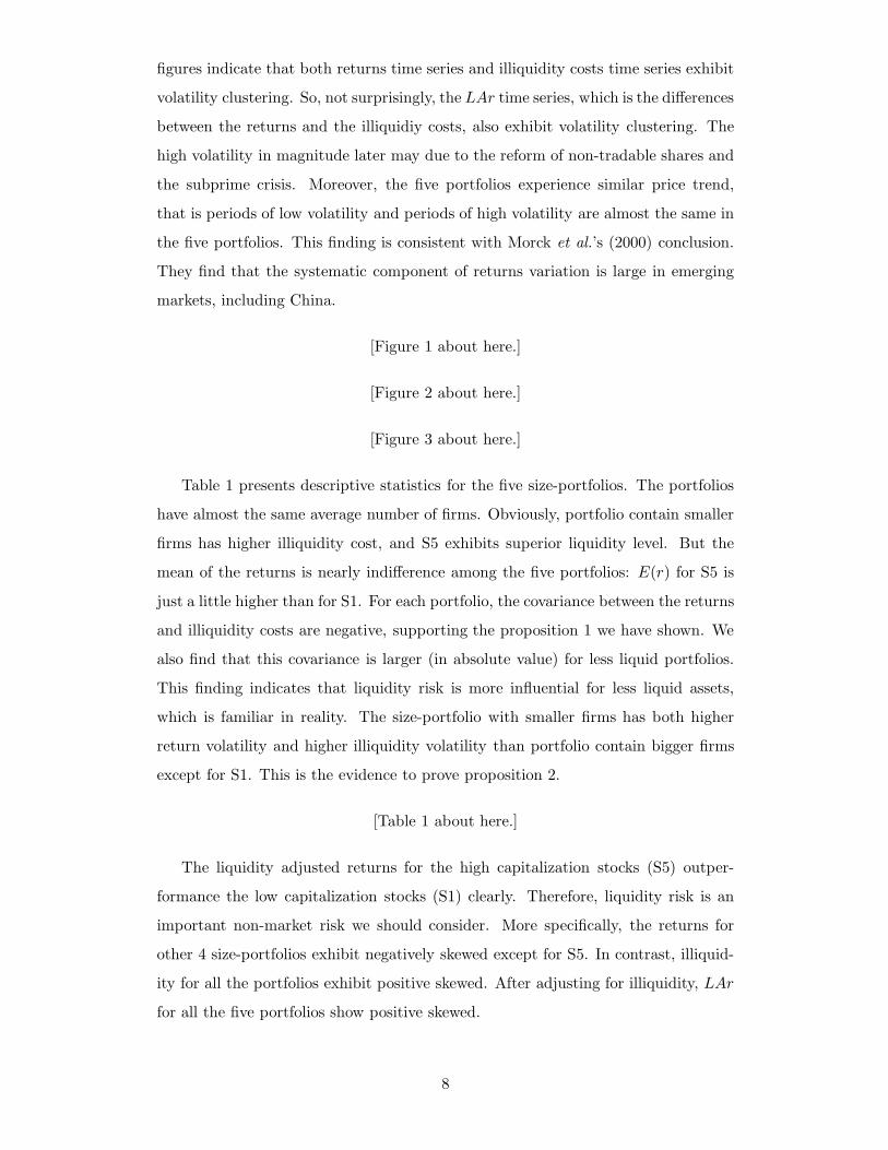
figures indicate that both returns time series and illiquidity costs time series exhibit

volatility clustering. So, not surprisingly, the LAr time series, which is the differences

between the returns and the illiquidiy costs, also exhibit volatility clustering. The

high volatility in magnitude later may due to the reform of non-tradable shares and

the subprime crisis. Moreover, the five portfolios experience similar price trend,

that is periods of low volatility and periods of high volatility are almost the same in

the five portfolios. This finding is consistent with Morck et al.’s (2000) conclusion.

They find that the systematic component of returns variation is large in emerging

markets, including China.

[Figure 1 about here.]



Table 1 presents descriptive statistics for the five size-portfolios. The portfolios

have almost the same average number of firms. Obviously, portfolio contain smaller

firms has higher illiquidity cost, and S5 exhibits superior liquidity level. But the

mean of the returns is nearly indifference among the five portfolios: E(r) for S5 is

just a little higher than for S1. For each portfolio, the covariance between the returns

and illiquidity costs are negative, supporting the proposition 1 we have shown. We

also find that this covariance is larger (in absolute value) for less liquid portfolios.

This finding indicates that liquidity risk is more influential for less liquid assets,

which is familiar in reality. The size-portfolio with smaller firms has both higher

return volatility and higher illiquidity volatility than portfolio contain bigger firms

except for S1. This is the evidence to prove proposition 2.

[Table 1 about here.]

The liquidity adjusted returns for the high capitalization stocks (S5) outper-

formance the low capitalization stocks (S1) clearly. Therefore, liquidity risk is an

important non-market risk we should consider. More specifically, the returns for

other 4 size-portfolios exhibit negatively skewed except for S5. In contrast, illiquid-

ity for all the portfolios exhibit positive skewed. After adjusting for illiquidity, LAr

for all the five portfolios show positive skewed.

8

3.3 Econometric models

VaR is an estimation of the tails of the empirical distribution (Angelidis et al.,

2004). The family of ARCH models are popularly used in modeling the daily VaR,

such as RiskMetricsTM or GARCH(1, 1) under specific distribution. We would also

use ARCH models in this study. Particularly, we set the conditional mean equation

by fitting an p orders autoregressive (AR(p)) process, that is

yt = φ0 +

p∑

i=1

φiy(t − i) + εt, (16)

where yt is the return series, illiquidity series or LAr series.

For many stocks, the “bad” news and the “good” news have different pronounced

effect on volatility— the so-called asymmetric effects. This asymmetric effects is

important in the accuracy of VaR estimation. Brooks and Persand (2003) find

that the VaR would be underestimated if the models leave asymmetric effects out

of account. Hence, we employ the GJR model, which was introduced by Glosten,

Jagannathan and Runkle (1993), to capture the asymmetric effects. On the other

hand, the Jarque-Bera tests in Tabel 1 show that all the series exhibit a non-normal

distribution. And all the series show either positively skewed or negatively skewed.

Therefore, to account for the non-normality and the excess skewness, we, follow

Giot and Laurent (2003), assume the residuals εt of the conditional mean equation

(16) have a skewed Student’s t-distribution. Finally, we set the conditional variance

equation to be a skewed Student’s t GJR model, that is

εt = σtzt (17)

σ2t = ω + α1ε

2t−1 + γ1λt−1ε

2t−1 + β1σ

2t−1, (18)

where λt is a dummy variable that take the value 1 when εt is negative and 0 when

it is positive. If γ1 > 0, negative shocks will have larger effects on volatility than

positive shocks— the so-called leverage effects.

Follow Lambert and Laurent (2001) and Giot and Laurent (2003), the innovation

process zt is assumed to be (standardized) skewed Student distributed, that is

f(z|ξ, ν) =

2

ξ + 1ξ

sg[ξ(sz + m)|ν], if z < −ms, (19)

2

ξ + 1ξ

sg[(sz + m)/ξ|ν], if z ≥ −ms, (19′)

9

where g(·|ν) is the standard Student’s t density with freedom ν and ξ is the asym-

metry coefficient: the density is skew to the right (left), if log(ξ) > 0(< 0)8. m

and s2 are respectively the mean and the variance of the non-standardized skewed

Student’t distribution:

m =Γ(

ν−12

)√ν − 2

√πΓ

(

ν2

) (ξ − 1

ξ), (20)

s2 =(

ξ2 +1

ξ2− 1

)

− m2. (21)

To estimate VaR, we need know the quantile function of the distribution. Lam-

bert and Laurent (2000) show that the quantile function of the standardized skewed

Student’s t distribution is

skstα,ν,ξ =skst∗α,ν,ξ − m

s, (22)

in which,

skst∗α,ν,ξ =

1

ξstα,ν[

α

2(1 + ξ2)], if α < 1

1+ξ2 , (23)

−ξstα,ν[1 − α

2(1 + ξ−2)], if α ≥ 1

1+ξ2 , (23′)

where stα,ν is the quantile function of the standard Student’s t density. Then given

confidence level 1 − α, the one-day-ahead VaR estimation is given by

V aRt(yt+1) = Et(yt+1) + skstα,ν,ξσt+1. (24)

4 Empirical results

Based on the estimation of the parametric model in subsection 3.3, we calculate

and compare the two kinds liquidity adjusted VaR— VaR(LAr), and the simply

adding of VaR(r) and VaR(−c). In addition, we will compute the liquidity compo-

nent in VaR(LAr) to highlight the importance of liquidity risk.

4.1 Skewed Student’s t AR-GJR model estimation

In this subsection, we firstly estimate the skewed Student’s t AR-GJR model (16)-

(21) for the five size-portfolios’ returns, illiquidity costs and LAr, respectively. All

the econometric models in this paper was estimated by G@RCH 5.0, an Ox package.

We only report the results for the volatility specification. Table 2 provides the

8See Giot and Laurent (2003) for a more detailed discussion.

10

parameters’ estimation for returns and illiquidity costs. we also compute the Pearson

correlation coefficient between the conditional variances of return and illiquidity.


The returns of five size-portfolios feature relatively similar volatility characteris-

tics. The conditional variances exhibit strong memory effects since the autoregressive

coefficient β1 is nearly 0.9. γ1 for returns is positive and significant for all portfolios,

which implies that the leverage effect for negative returns also exists in China’s stock

market. log(ξ) is negative for all portfolios and significant except for S5, indicating

a negative excess skewness.

For the illiquidity costs, memory effects of the conditional variance also exist in

each portfolio. But S5 show a high sensitivity to short run shock (α1 = 0.883). log(ξ)

is positive and significant for all portfolios, indicating a positive excess skewness. γ1

is negative and significant for each portfolio. Notice that a negative illiquidity shock

equal to a positive liquidity shock. Hence, there also exist a leverage effect for

negative liquidity shocks. Moreover, the absolute value of γ1 for illiquidity costs is

much larger than for returns, which implies that liquidity is much more sensitive.

The bankruptcy of LTCM is a suitable example. “. . . LTCM’s partners, calling in

from Tokyo and London, reported that their markets has dried up. There were no

buyers, no sellers. . . . ”9.

The Pearson correlation coefficient between the conditional variances of returns

and illiquidity costs is positive for all portfolios, supporting the proposition 2 we

have proved. Moreover, this correlation coefficient is larger for less liquid portfolios,

indicating that liquidity risk is more influential for less liquid assets, similar to the

conclusion in table 1.

Table 3 presents the estimation results for the conditional variance models of

LAr. All the portfolios exhibit relatively similar volatility characteristics for LAr.

The autoregressive coefficient β1 is close to 0.9, pointing out a memory effect of the

conditional variance for LAr. γ1 for LAr is positive and significant for each portfolio,

indicating a leverage effect for negative LAr in the conditional variance specification.

log(ξ) is negative and significant for all portfolios, which implies a negative excess

skewness.


9Wall Street Journal, November 16, 1998.

11

4.2 Liquidity adjusted VaR

In this subsection, we calculate and compare the two kinds one-day-ahead liq-

uidity adjusted VaR— VaR(LAr), and the simply adding of VaR(r) and VaR(−c).

We will also compute the liquidity component ℓ in equation (10) to emphasize the

importance of liquidity risk.

Table 4 provides that two kinds one-day-ahead liquidity adjusted VaR and the

liquidity component ℓ given α = 5% or 1% ( the confidence level 1 − α is 95% or

99%). We find that, without adjusting for liquidity risk, the VaR(r) is relatively

similar for S1, S2, S3 and S4. S5 has a smaller VaR(r). But after incorporating

liquidity risk in VaR, VaR(LAr) is larger for more illiquidity (lower capitalized)

portfolio. Also, S5 is much outperformance S1: the difference between VaR(LAr)

of S1 and S5 is 1.583 percent when α = 5% or 2.371 percent when α = 1%, but it

is 0.523 or 0.675 for VaR(r). Moreover, the liquidity component ℓ is more than 22%

for the low capitalization portfolios and almost 5% even for the high capitalization

ones. All the above results indicate that liquidity risk is even more important and

we must incorporate the liquidity risk in VaR measure.


By comparing VaR(LAr) with VaR(r)+VaR(−c), we find that VaR(LAr) is a

little larger than the simply adding for all portfolios whenever α = 5% or 1%. It

appears that the simply adding VaR(r)+VaR(−c) underestimates the risk. How-

ever, we couldn’t make the final judgement before testing the accuracy of the two

approaches. We will do the test in next subsection.

4.3 Accuracy testing

The accuracy testing is based on the statistic developed by Kupiec (1995). For

a T -day period, suppose N is the number of empirical failure days, which is the

number returns exceed (in absolute value) the forecasted VaR. If the VaR model

is correctly specified, N/T should be equal to the theoretical specified VaR level

α. Then the appropriate likelihood ratio statistic, under the null hypothesis that

N/T = α, is:

LRuc = −2[

log(

(1 − α)T−NαN)

− log(

(1 − N

T)T−N (

N

T)N

)]

∼ χ21 (25)

Table 5 presents the number of failure days for the two kinds liquidity adjusted

VaR model — VaR(LAr) and VaR(r)+VaR(−c) — for each portfolio in the sample

12

period. Based on equation (25), the 95% confidence intervals of the number of failure

days are (77.82, 115.38) and (10.75, 27.89) for α = 5% and α = 1%, respectively. In

all portfolios, whenever α = 5% or 1%, the number of failure days of the VaR(LAr)

model is closer to the theoretical number than the model of simply adding. Generally,

at the 95% confidence level, VaR(LAr) are more accurate than VaR(r)+VaR(−c),

even though the method of simply adding also generates adequate risk predictions.


In addition, the number of failure days predicted by VaR(r)+VaR(−c) are closer

to the expected number for S5 both at α = 5% and α = 1%. This finding supports

our arguments that the relationships between liquidity risk and market risk produce

the inaccuracy of the method of simply adding. In fact, we find that the negative

covariance and the positive correlation between returns and illiquidity costs, which

are the causations of the inaccuracy of the VaR(r)+VaR(−c) model, both are the

smallest (in absolute value) for S5 in table 1 and table 2. Then it is not surprising

that VaR(r)+VaR(−c) could predict more precise number of failure days for S5 than

for other portfolios.

5 Conclusions

In this paper, by simplifying Acharya and Pedersen’s (2006) overlapping gener-

ation model, we show that liquidity risk could influence the market risk forecasting

through two ways. Then the accuracy of the traditional liquidity adjusted VaR mea-

sure, the simply adding of the two risk measure, would also be influenced through

two ways: 1) First, returns are low when illiquidity increases. Therefore, the value

at market risk would increase and the simply adding would underestimate the risk.

2) Second, we show that the volatility of returns would be amplified if the volatility

of illiquidity risk is large. Then the value at market risk would also increase and the

simply adding would underestimate the risk, too. At a word, just add the two risk

measure would underestimate the liquidity adjusted VaR.

Hence, we employ another method to incorporate liquidity risk in VaR measure.

We modeling the liquidity adjusted returns (LAr) directly, where the LAr is equal

to returns minus illiquidity cost. Under such an approach, China’s stock market is

specifically studied. We first construct a skewed Student’s t AR-GJR model to cap-

ture the asymmetric effect, non-normality and excess skewness of return, illiquidity

13

and LAr. Then we estimate the one-day-ahead “standard” VaR and liquidity ad-

justed VaR. We find that for the most illiquidity portfolio, liquidity risk represents

more than 22% of total risk. We also find that simply adding of the two risk mea-

sure would underestimate the risk. The accuracy testing based on Kupiec’s (1995)

statistic show that our approach is more accurate than the method of simply adding.

The findings of this paper make three main contributions to literatures. Firstly,

we propose a more accurate approach to modeling liquidity adjusted VaR. Secondly,

this study adds to the evidence on the importance of liquidity risk in VaR measure.

Lastly, there are rarely studies considering China’s stock market about such issue in

international journals. But China has became the most important emerging market

and its stock market has been opened to international investors. Hence we need

more researches, such as this paper, to study the characteristic of the risk in China’s

stock market.

Appendix

We first solve the problem of investor n at time t. We assume the investor n

purchases yn shares of the risky asset. Then the agent’s problem is

maxyn∈R+

Et(Wnt+1) −

1

2γV art(W

nt+1), (A.1)

where

W nt+1 = (Pt+1 − Ct+1)y

n + Rf (ent − Pty

n). (A.2)

From the first order condition, we have

yn =1

γ[V art(Pt+1 − Ct+1)]

−1[Et(Pt+1 − Ct+1) − RfPt]. (A.3)

Since the total supply of risky asset S =∑

n yn, then we have equilibrium conditon

Pt =1

Rf[Et(Pt+1 − Ct+1) −

γS

NV art(Pt+1 − Ct+1)]. (A.4)

We can obtain the unique stationary linear equilibrium,

Pt = Υ + ΦCt, (A.5)

14

where

Υ = − 1

Rf − 1

[Rf (1 − ρC)

Rf − ρCC +

γS

NV art(−

Rf

RF − ρCηt)

]

, (A.6)

Φ = − ρC

Rf − ρC. (A.7)

Proof of Proposition 1

The conditional covariance between illiquidity and the gross return is

Covt(ct+1, Rt+1) =1

P 2t

Covt(Ct+1, Pt+1)

=1

P 2t

Covt

(

Ct+1,−ρC

Rf − ρCCt+1

)

=1

P 2t

(

− ρC

Rf − ρC

)

V art(Ct+1)

< 0, (A.8)

which yields the proposition. 2

Proof of Proposition 2

The conditional variance of the gross return is

V art(Rt+1) =1

P 2t

V art(Pt+1)

=1

P 2t

V art

(

− ρC

Rf − ρCCt+1

)

=1

P 2t

( ρC

Rf − ρC

)2V art(Ct+1). (A.9)

So we have

∂V art(Rt+1)

∂V art(Ct+1)=

1

P 2t

( ρC

Rf − ρC

)2> 0, (A.10)

which yields the proposition. 2

15

References

Acharya, V. V. and L. H. Pedersen, 2005. Asset pricing with liquidity risk. Journal

of Financial Economics, 77(2), 375–410.

Amihud, Y., 2002. Illiquidity and stock returns: cross-section and time-series effects.

Journal of Financial Markets, 5(1), 31–56.

Amihud, Y. and H. Mendelson, 1986. Asset pricing and the bid-ask spread. Journal

of Financial Economics, 17(2), 223–249.

Angelidis, T. and A. Benos, 2006. Liquidity adjusted value-at-risk based on the

components of the bid-ask spread. Applied Financial Economics, 16(11), 835 –

851.

Angelidis, T., A. Benos, and S. Degiannakis, 2004. The use of GARCH models in

VaR estimation. Statistical Methodology, 1(1-2), 105–128.

Artzner, P., F. Delbaen, J.-M. Eber, and D. Heath, 1999. Coherent measures of risk.

Mathematical Finance, 9(3), 203–228.

Bangia, A., F. X. Diebold, T. Schuermann, and J. Stroughair, 1999. Modeling

liquidity risk with implications for traditional market risk measurement and man-

agement.

Bekaert, G., C. R. Harvey, and C. Lundblad, 2007. Liquidity and expected returns:

lessons from emerging markets. Review of Financial Study, 20(6), 1783–1831.

Brennan, M. J., T. Chordia, and A. Subrahmanyam, 1998. Alternative factor speci-

fications, security characteristics, and the cross-section of expected stock returns.

Journal of Financial Economics, 49(3), 345–373.

Brooks, C. and G. Persand, 2003. The effect of asymmetries on stock index return

Value-at-Risk estimates. The Journal of Risk Finance, 4(2), 29–42.

Giot, P. and S. Laurent, 2003. Value-at-Risk for long and short trading positions.

Journal of Applied Econometrics, 18(6), 641–664.

Glosten, L. R., R. Jagannathan, and D. E. Runkle, 1993. On the relation between

the rxpected value and the volatility of the nominal excess return on stocks. The

Journal of Finance, 48(5), 1779–1801.

16

Hasbrouck, J., 2002. Inferring trading costs from daily data: US equities from 1962

to 2001. Unpublished working paper.

Holmstrom, B. and J. Tirole, 2001. LAPM: A liquidity-based asset pricing model.

The Journal of Finance, 56(5), 1837–1867.

Kupiec, P. H., 1995. Techniques for verifying the accuracy of risk measurement

models. The Journal of Derivatives, (3), 73–84.

Kyle, A. S., 1985. Continuous auctions and insider trading. Econometrica, 53(6),

1315–1335.

Lambert, P. and S. Laurent, 2000. Modelling skewness dynamics in series of financial

data. Unpublished working paper.

Lambert, P. and S. Laurent, 2001. Modelling financial time series using GARCH-

type models and a skewed Student density. Unpublished working paper.

Liu, W., 2006. A liquidity-augmented capital asset pricing model. Journal of Fi-

nancial Economics, 82(3), 631–671.

Morck, R., B. Yeung, and W. Yu, 2000. The information content of stock markets:

why do emerging markets have synchronous stock price movements? Journal of

Financial Economics, 58(1-2), 215–260.

Pastor, L. and R. F. Stambaugh, 2003. Liquidity risk and expected stock returns.

Journal of Political Economy, 111(3), 642–685.

17

0 300 600 900 1200 1500 1800

−5

0

5

10

r_S1 0 300 600 900 1200 1500 1800

0

10

r_S2

0 300 600 900 1200 1500 1800

0

10

r_S3 0 300 600 900 1200 1500 1800

0

10

r_S4

0 300 600 900 1200 1500 1800

0

10

r_S5

Figure 1. Daily Returns (in percent) of size-portfolios (from small to big: S1, S2,S3, S4 and S5) from 2 January 2001 to 31 December 2008.

18

0 300 600 900 1200 1500 1800

2

4

c_S1 0 300 600 900 1200 1500 1800

1

2

3

4

c_S2

0 300 600 900 1200 1500 1800

1

2

c_S3 0 300 600 900 1200 1500 1800

0.5

1.0

1.5

c_S4

0 300 600 900 1200 1500 1800

0.2

0.4

c_S5

Figure 2. Daily illiquidity costs (in percent) of size-portfolios (from small to big: S1,S2, S3, S4 and S5) from 2 January 2001 to 31 December 2008.

19

0 300 600 900 1200 1500 1800

−10

0

10

LAr_S1 0 300 600 900 1200 1500 1800

−10

0

10

LAr_S2

0 300 600 900 1200 1500 1800

−10

0

10

LAr_S3

0 300 600 900 1200 1500 1800

0

10

LAr_S4

0 300 600 900 1200 1500 1800

0

10

LAr_S5

Figure 3. Daily Liquidity adjusted returns (LAr, in percent) of size-portfolios (fromsmall to big: S1, S2, S3, S4 and S5) from 2 January 2001 to 31 December 2008.

20

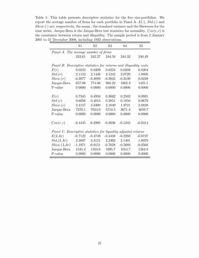
Table 1: This table presents descriptive statistics for the five size-portfolios. Wereport the average number of firms for each portfolio in Panel A. E(·), Std.(·) andSkew.(·) are, respectively, the mean , the standard variance and the Skewness for thetime series. Jarque-Bera is the Jarque-Bera test statistics for normality. Cov(r, c) isthe covariance between return and illiquidity. The sample period is from 2 January2001 to 31 December 2008, including 1932 observations.

S1 S2 S3 S4 S5

Panel A. The average number of firms

233.61 242.27 244.50 244.32 240.49

Panel B. Descriptive statistics for returns and illiquidity costs

E(r) 0.0222 0.0209 0.0224 0.0208 0.0204Std.(r) 2.1152 2.1446 2.1242 2.0729 1.8800Skew.(r) -0.3977 -0.3889 -0.3835 -0.3139 0.0228Jarque-Bera 657.08 774.06 988.22 1062.3 1425.1P-value 0.0000 0.0000 0.0000 0.0000 0.0000

E(c) 0.7345 0.4958 0.3662 0.2502 0.0931Std.(c) 0.6056 0.4015 0.2851 0.1850 0.0679Skew.(c) 2.4157 2.3300 2.1649 1.9721 2.0828Jarque-Bera 7270.1 7024.0 5710.5 3671.3 4659.7P-value 0.0000 0.0000 0.0000 0.0000 0.0000

Cov(r, c) -0.4445 -0.2995 -0.2036 -0.1245 -0.0314

Panel C. Descriptive statistics for liquidity adjusted returns

E(LAr) -0.7122 -0.4749 -0.3438 -0.2293 -0.0727Std.(LAr) 2.3937 2.3151 2.2362 2.1401 1.8979Skew.(LAr) -1.1971 -0.9151 -0.7628 -0.5689 -0.0568Jarque-Bera 1545.4 1104.6 1095.7 1014.7 1284.8P-value 0.0000 0.0000 0.0000 0.0000 0.0000

21

Table 2: This table presents the estimation results for the conditional variance models of returns and illiquidity costs. Robust standard errorsare reported in parentheses. Corr(σ2

r , σ2c ) is the Pearson correlation coefficient between the conditional variances of returns and illiquidity. The

sample period is from 2 January 2001 to 31 December 2008, including 1932 observations.

S1 S2 S3 S4 S5y r c r c r c r c r c

ω 0.062(0.024) 0.002(0.001) 0.051(0.021) 0.001(0.000) 0.042(0.017) 0.001(0.000) 0.037(0.016) 0.000(0.000) 0.031(0.013) 0.001(0.051)α1 0.093(0.023) 0.242(0.030) 0.092(0.022) 0.235(0.027) 0.089(0.021) 0.228(0.025) 0.085(0.021) 0.218(0.025) 0.069(0.017) 0.443(0.067)β1 0.878(0.023) 0.856(0.016) 0.883(0.020) 0.868(0.014) 0.887(0.018) 0.869(0.013) 0.889(0.018) 0.876(0.014) 0.899(0.017) 0.777(0.024)γ1 0.045(0.022) -0.324(0.040) 0.050(0.022) -0.358(0.038) 0.052(0.022) -0.342(0.036) 0.060(0.023) -0.335(0.032) 0.070(0.023) -0.441(0.066)log(ξ) -0.174(0.029) 0.602(0.054) -0.162(0.028) 0.610(0.048) -0.142(0.029) 0.615(0.041) -0.128(0.028) 0.629(0.038) -0.032(0.029) 0.548(0.035)ν 6.827(1.095) 4.251(0.411) 5.212(0.654) 4.240(0.403) 5.769(0.804) 4.167(0.395) 5.560(0.748) 4.133(0.381) 5.212(0.654) 2.527(0.025)

Corr(σ2r, σ2

c) 0.660 0.576 0.543 0.536 0.256

Log-likelihood -3883.364 37.526 -3882.678 688.234 -3831.761 1265.413 -3773.060 2069.560 -3575.176 3787.696

22

Table 3: This table presents the estimation results for the conditional variance modelof LAr. Robust standard errors are reported in parentheses. The sample period isfrom 2 January 2001 to 31 December 2008, including 1932 observations.

S1 S2 S3 S4 S5

ω 0.117(0.038) 0.079(0.027) 0.059(0.021) 0.046(0.018) 0.033(0.014)α1 0.092(0.030) 0.091(0.027) 0.088(0.024) 0.083(0.023) 0.067(0.017)β1 0.870(0.024) 0.880(0.021) 0.885(0.019) 0.887(0.018) 0.897(0.017)γ1 0.039(0.033) 0.043(0.029) 0.047(0.026) 0.060(0.026) 0.074(0.025)log(ξ) -0.364(0.030) -0.299(0.028) -0.252(0.029) -0.203(0.029) -0.056(0.029)ν 5.693(0.777) 5.742(0.825) 5.827(0.846) 5.678(0.794) 5.298(0.687)

Log-likelihood -3995.937 -3968.288 -3901.662 -3819.144 -3594.588

23

Table 4: This table presents the one-day-ahead liquidity adjusted VaR and the liq-uidity component ℓ. VaR(r) is the one-day-ahead VaR without considering liquidityrisk; VaR(LAr) is the liquidity adjusted VaR based on liquidity adjusted returns;the simply adding of VaR(r) and VaR(−c) is denoted as VaR(r)+VaR(−c).

S1 S2 S3 S4 S5

α = 5% VaR(r) 4.410 4.347 4.500 4.382 3.887VaR(LAr) 5.713 5.363 5.325 4.958 4.130ℓ 22.8% 18.9% 15.5% 11.6% 5.88%VaR(r)+VaR(−c) 5.659 5.343 5.215 4.888 4.022

α = 1% VaR(r) 7.118 7.152 7.452 7.280 6.443VaR(LAr) 9.151 8.665 8.652 8.123 6.780ℓ 22.2% 17.5% 13.9% 10.4% 4.97%VaR(r)+VaR(−c) 8.863 8.557 8.466 7.997 6.667

24

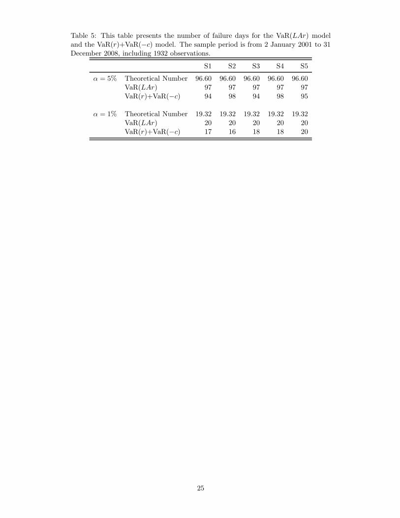
Table 5: This table presents the number of failure days for the VaR(LAr) modeland the VaR(r)+VaR(−c) model. The sample period is from 2 January 2001 to 31December 2008, including 1932 observations.

S1 S2 S3 S4 S5

α = 5% Theoretical Number 96.60 96.60 96.60 96.60 96.60VaR(LAr) 97 97 97 97 97VaR(r)+VaR(−c) 94 98 94 98 95

α = 1% Theoretical Number 19.32 19.32 19.32 19.32 19.32VaR(LAr) 20 20 20 20 20VaR(r)+VaR(−c) 17 16 18 18 20

25

Incorporating Liquidity Risk in Value ... -...

Documents

Transcript of Incorporating Liquidity Risk in Value ... -...