Incorporating Climate Change into the Design of

Water Crossing Structures

Washington Department of Fish and Wildlife in Cooperation with the Climate Impacts Group, University of Washington, with funding support

provided by the North Pacific Landscape Conservation Cooperative

FINAL PROJECT REPORT October 2016

George Wilhere (WDFW) Jane Atha (WDFW) Timothy Quinn (WDFW) Lynn Helbrecht (WDFW) Ingrid Tohver (Climate Impacts Group)

Figure 19 - Page 30

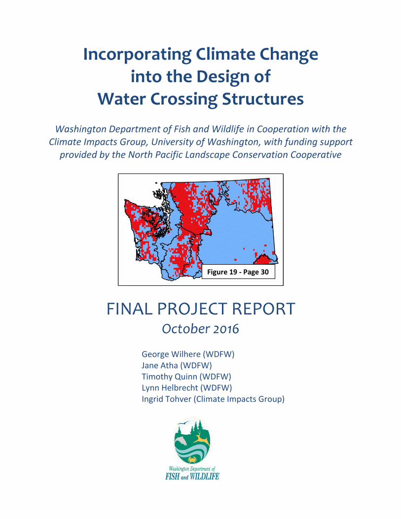
Incorporating Climate Change into the

Design of Water Crossing Structures

Table of Contents

1. Introduction ........................................................................................................................ 1 The Importance of Water Crossing Structures ..................................................................................... 1

Culvert Design ....................................................................................................................................... 2

Hydraulic Geometry .............................................................................................................................. 4

Climate Change Impacts on Stream Hydrology and Channel Morphology .......................................... 5

Addressing Climate Change Impacts to Fish Passage ........................................................................... 7

2. Methods − Projecting Future Bankfull Flows and Bankfull Widths ........................................ 8 Global Climate Models .......................................................................................................................... 8

VIC Hydrologic Model ......................................................................................................................... 11

Projected Streamflow Analyses .......................................................................................................... 13

Estimating Change in Bankfull Width.................................................................................................. 15

100-Year Flood Analysis ...................................................................................................................... 15

3. Results .............................................................................................................................. 17 Projected Changes in Bankfull Width ................................................................................................. 17

100-Flood Analysis .............................................................................................................................. 21

4. Information for Culvert Design ........................................................................................... 24 Uncertainty ......................................................................................................................................... 24

Risk and Actionable Risk .................................................................................................................... 24

Case Study: Climate-adapted Culverts for the Chehalis River Basin .................................................. 31

5. Discussion ......................................................................................................................... 37

6. Future Work ...................................................................................................................... 39 Dissemination of Project Results ........................................................................................................ 39

Updating Climate Science ................................................................................................................... 39

Understanding the Consequences of Undersized Culverts ................................................................ 40

Improving Information on risk and cost ............................................................................................. 40

7. Acknowledgements ........................................................................................................... 40

8. References ........................................................................................................................ 41

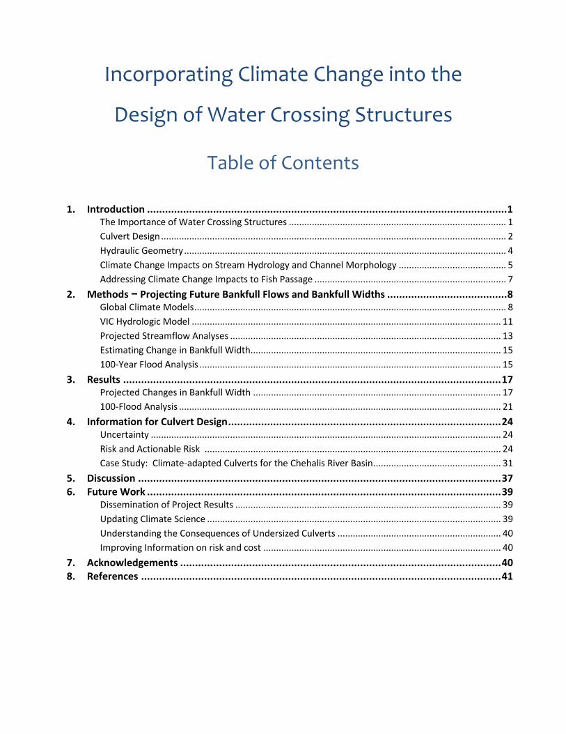
Figures Figure 1. The width of no-slope and stream simulation culverts compared to bankfull width. ................. 3

Figure 2. Causal relationships between culverts and climate change. ........................................................ 7

Figure 3. Major steps in the modelling process. ........................................................................................ 8

Figure 4. Future greenhouse gas scenarios ............................................................................................... 11

Figure 5. Components and modelled processes of the VIC hydrologic model. ......................................... 12

Figure 6. Validation of VIC streamflow estimates using ratio of 100-year flood and mean annual flood. 13

Figure 7. Three major ecoregion divisions used to assign bankfull flow recurrence intervals .................. 16

Figure 8. Frequency distribution of grid cells for mean projected percent change in bankfull width). .... 19

Figure 9. Coefficient of variation for 10 bankfull width projections versus mean percent change in

bankfull width for each of the 5270 grid cells. .......................................................................................... 19

Figure 10. The mean (of 10 models) projected percent change in bankfull width ................................... 20

Figure 11. Projected future mean % change in 100-year flood volume (Q100) relative to historical Q100 . 21

Figure 12. Frequency distribution of grid cells for mean projected percent change in 100-year flood .... 22

Figure 13. The distribution of grid cells within ecoregions for ratio of percent change in 100-year flood

volume to percent change in bankfull width .............................................................................................. 23

Figure 14. The ratio of percent change in 100-year flood volume to percent change in bankfull width .. 23

Figure 15. The range of percent change in bankfull width for each grid cell ............................................ 27

Figure 16. Number of models projecting an increase in bankfull width for each grid cell ........................ 28

Figure 17. Distribution of projected percent change in bankfull width (BFW) between historical and

2040s time periods ..................................................................................................................................... 29

Figure 18. Graphical depiction of relative risk. ........................................................................................ 30

Figure 19. Grid cells that lie within the actionable risk zone of Figure 18. . ............................................. 30

Figure 20. Grid cells on nonfederal lands where a culvert poses an actionable risk ................................. 31

Figure 21. The Polson Camp Road Culvert Project on Big Creek, a tributary of the Humptulips River. .. 33

Figure 22. Distribution of projected future percent change in bankfull widths and future bankfull width

for the Polson Camp Road Culvert Project on Big Creek (see Figure 21). ................................................. 34

Figure 23. Distribution of projected percent change in 100-year flood volume relative to the historical

estimate for the Polson Camp Road Culvert Project on Big Creek (see Figure 21). .................................. 35

Figure 24. Smallest current bankfull width (in feet) where a bridge (rather than a culvert) may be

warranted based on mean projected percent change in bankfull width ................................................... 36

Figure 25. Percent increase in culvert cost as a function of percent increase in culvert width. ............. 39

Tables Table 1. Ten global climate models used to project stream flows in the Pacific Northwest. ................... 10

Table 2. Downstream hydraulic geometry parameters from Castro and Jackson (2001). ...................... 16

Table 3. Mean percent change from historical to future projections of bankfull discharge………………… 18

Table 4. Example of how relative risk could be mapped for policy decisions. .......................................... 31

1

1. Introduction

The following report describes a study conducted by the Washington Department of Fish and Wildlife (WDFW or the Department) from 2014 to 2016. The study represents the Department’s initial attempt to explore climate-related changes to stream channel morphology with the intent of determining how climate change could be incorporated into the design of water crossing structures. The Department received a grant from the North Pacific Landscape Conservation Cooperative (NPLCC) that provided essential support for this work. This report fulfills a required deliverable of that grant. Using this Report Please note that this report is presented as informational only. It is intended to provide information that managers or engineers might consider when designing new or replacement water crossing structures. Use of this report and the information it provides is voluntary. Section 1 explains the importance of properly designed water crossing structures for fish movement, the basics of geomorphic culvert design, basics of channel hydraulic geometry, the projected impacts of future climate change on stream hydrology and channel morphology in Washington, and the motivations for this project. Section 2 describes our methods for translating climate projections to the key geomorphological parameter used in culvert design and permitting, and Section 3 presents the results and findings from our work. Section 4 explains how the information we have produced can be used for culvert design. Section 5 is a discussion of our results and the challenges of incorporating our projections into culvert design. Finally, Section 6 describes additional work needed to better address the information needs of policy makers, managers, and engineers.

The Importance of Water Crossing Structures Washington State regulations require that water crossing structures (i.e., culverts and bridges) “allow fish to move freely through them at all flows when fish are expected to move” (WAC 220-660-190). Furthermore, Washington State law (RCW 77.57) grants WDFW authority to regulate the construction of water crossing structures along with other activities that use, obstruct, divert, or change the natural flow or bed of state waters. The Department issues approximately 400 permits per year related to water crossings throughout the state (WDFW 2006). In addition, the Department designs or co-designs water crossing structures throughout the state and provides technical guidance (Barnard et al. 2013) that explains how to design water crossing structures that will comply with current regulations. Road crossings at rivers or streams are widely known to create barriers to fish movement when they are improperly designed or constructed (Price et al. 2010, Chelgren and Dunham 2015). Improperly designed or constructed culverts can become barriers for various reasons, including sediment aggradation at a culvert’s inlet, stream bed scour at a culvert’s outlet, and high flow velocity in the culvert . The consequences to fish populations associated with barriers at road crossings include the loss of habitat for various life history stages (Beechie et al. 2006, Sheer and Steel 2006), genetic isolation (Reiman and Dunham 2000, Wofford et al. 2005, Neville et al. 2009), inaccessibility to refuge habitats during disturbance events or warm water episodes (Lamberti et al. 1991, Reeves et al. 1995, Dunham et al. 1997), and local extirpation (Winston et al. 1991, Kruse et al. 2001). The importance of restoring fish passage at water crossings in Washington has been highlighted with Washington’s Salmon Recovery Act of 1998, the Forests and Fish Report (DNR 1999), and United States v. Washington (2013), which is also known as the “Culvert Case.” All regional recovery plans for salmon (Oncorhynchus spp.) in Washington State emphasize the importance of restoring fish passage at stream crossings for recovering federally-listed threatened salmon populations. Likewise, under the Forests and

2

Fish rules (WAC 222-24-051), large forest landowners are required to repair or replace all fish passage barriers before November 2016. Between 1999 and 2008, forest landowners replaced 3,500 fish passage barrier culverts with fish-passable structures, reportedly opening nearly 3,700 miles of fish habitat in Washington streams (Governor’s Salmon Recovery Office 2008). In the Culvert Case, Washington State government was ordered by a federal court to replace state-owned roadway culverts located on the Olympic Peninsula, in the Puget Sound Basin, or in the Chehalis River Basin that block salmon habitat (United States v. Washington 2013). About 1000 culverts are estimated to fit that description, and their replacement with culverts that pass fish is estimated to cost about $2.45 billion (Lovaas 2013). Recent studies describe the magnitude of the challenge presented by culverts both in terms of the sheer number of structures across the landscape and in the proportion of those culverts that may be barriers to fish passage. The U.S. Forest Service and Bureau of Land Management reported that over half of the estimated 10,215 culverts that exist on fish-bearing streams in federal lands of Washington and Oregon may be fish passage barriers (GAO 2001). The Washington State Department of Transportation (WSDOT) is responsible for about 3,000 culverts on fish-bearing streams, of which approximately 60% are complete or partial barriers (WDFW 2009). In 2015, WDFW estimated that there may be as many as 35,000 culverts blocking or impeding fish passage statewide (D. Price, WDFW, personal communication). The goal of WDFW, WSDOT, other state agencies, and tribes is to restore access to existing freshwater habitat by replacing all impassable culverts. Hence, over the coming decades thousands of culverts must be replaced. The cost to replace 35,000 culverts could be as much as $60 to $86 billion.

Culvert Design WDFW has published water crossing design guidelines (i.e., Barnard et al. 2013) that are used by state and local governments throughout the United States (NAACC 2016, USACE 2016). WDFW, nationally recognized as the inventor of the stream simulation culvert design (Cenderelli et al. 2011), believes that a geomorphic approach to culvert design is the best way to enable upstream and downstream movements of fish and other stream-associated species through culverts (Barnard et al 2013). A geomorphic culvert design seeks to maintain continuity of channel structure and composition by conveying water, sediment, and wood in the same way as the surrounding stream reach (Barnard et al 2013, Cenderelli et al. 2011). In contrast, the once prevalent hydraulic culvert design viewed culverts as simply pipes for conveying water, and fish passage was accommodated by limiting flow velocities within the pipe. Culverts based on a geomorphic design: i) are large enough to accommodate regular flood flows, ii) contain deformable channel beds with a shape and sediments resembling the up- and downstream channel, and iii) have channel beds similar in slope to the longitudinal profile of the channel reach.

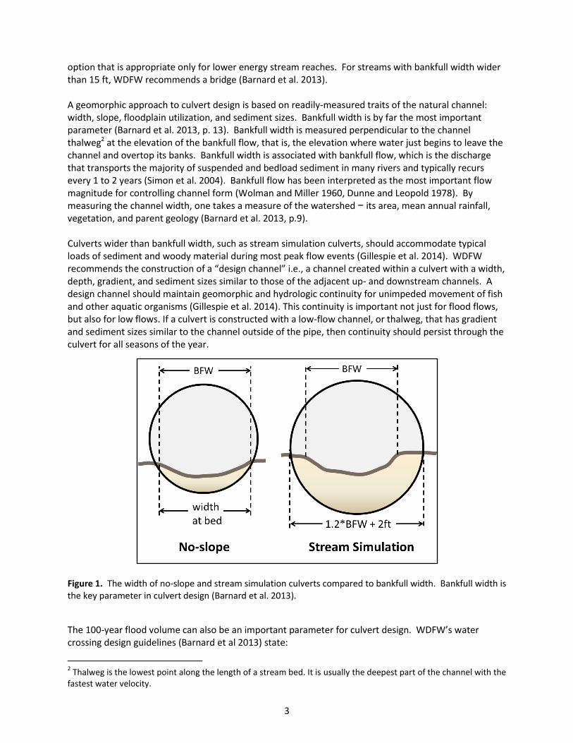
The Department currently endorses two types of culvert design: no-slope and stream simulation (Figure 1). The no-slope culvert is intended to be installed at 0% slope in small, low gradient streams (< 10 ft bankfull width, < 3% slope). No-slope culverts are countersunk1 to a minimum depth of 20% of the culvert height and the width of the no-slope culvert at the streambed elevation is at least bankfull width. Stream simulation culverts are intended for higher gradients and streams up to 15 ft bankfull width, and are sized to be 1.2 × bankfull width + 2 ft wide at the streambed and countersunk 30 to 50%. Stream simulation design is based on the assumption that if fish can migrate through the natural channel, then fish should also be able to migrate through an artificial channel that closely simulates the composition, structure, and fluvial processes of the natural channel. No-slope design is a less expensive

1 A countersunk culvert is installed with its bottom (i.e., invert) located below the existing channel elevation and

then filled with streambed material.

3

option that is appropriate only for lower energy stream reaches. For streams with bankfull width wider than 15 ft, WDFW recommends a bridge (Barnard et al. 2013). A geomorphic approach to culvert design is based on readily-measured traits of the natural channel: width, slope, floodplain utilization, and sediment sizes. Bankfull width is by far the most important parameter (Barnard et al. 2013, p. 13). Bankfull width is measured perpendicular to the channel thalweg2 at the elevation of the bankfull flow, that is, the elevation where water just begins to leave the channel and overtop its banks. Bankfull width is associated with bankfull flow, which is the discharge that transports the majority of suspended and bedload sediment in many rivers and typically recurs every 1 to 2 years (Simon et al. 2004). Bankfull flow has been interpreted as the most important flow magnitude for controlling channel form (Wolman and Miller 1960, Dunne and Leopold 1978). By measuring the channel width, one takes a measure of the watershed − its area, mean annual rainfall, vegetation, and parent geology (Barnard et al. 2013, p.9). Culverts wider than bankfull width, such as stream simulation culverts, should accommodate typical loads of sediment and woody material during most peak flow events (Gillespie et al. 2014). WDFW recommends the construction of a “design channel” i.e., a channel created within a culvert with a width, depth, gradient, and sediment sizes similar to those of the adjacent up- and downstream channels. A design channel should maintain geomorphic and hydrologic continuity for unimpeded movement of fish and other aquatic organisms (Gillespie et al. 2014). This continuity is important not just for flood flows, but also for low flows. If a culvert is constructed with a low-flow channel, or thalweg, that has gradient and sediment sizes similar to the channel outside of the pipe, then continuity should persist through the culvert for all seasons of the year. Figure 1. The width of no-slope and stream simulation culverts compared to bankfull width. Bankfull width is the key parameter in culvert design (Barnard et al. 2013).

The 100-year flood volume can also be an important parameter for culvert design. WDFW’s water crossing design guidelines (Barnard et al 2013) state:

2 Thalweg is the lowest point along the length of a stream bed. It is usually the deepest part of the channel with the

fastest water velocity.

4

“The standard of practice for culvert design dictates that the structure remains safe and serviceable up to a given design flood. WAC 220-110-070(3)(d) requires that the culvert must maintain structural integrity to the 100-year peak flow with consideration of debris likely to be encountered. Generally, sizing culverts using the no-slope method provides adequate conveyance for the 100-year peak flow. This does not absolve the designer of responsibility to determine that this is actually true.”3

The stream simulation culvert design is also assumed to provide adequate conveyance for the 100-year peak flow, and therefore, potential impacts of 100-year flood events are typically not an important design consideration. However, if a culvert is in a narrowly confined channel, likely to transport large woody debris, or downstream of high run-off areas (e.g., urban areas), then the designer should assess the potential impacts of 100-year flood events.

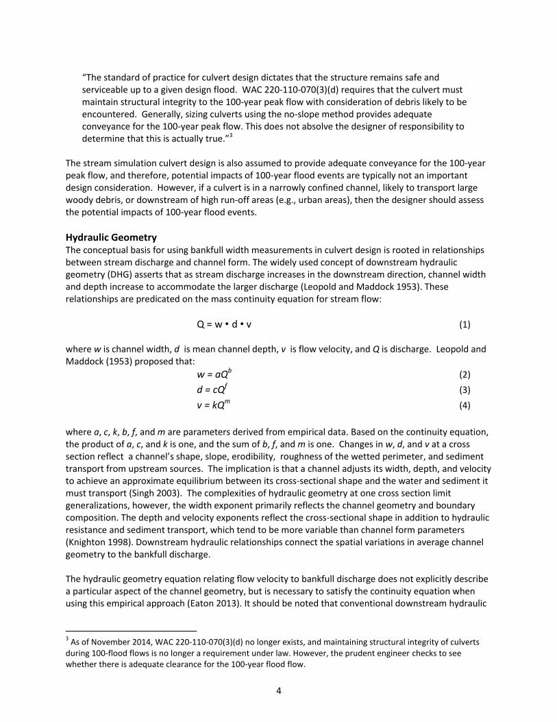
Hydraulic Geometry The conceptual basis for using bankfull width measurements in culvert design is rooted in relationships between stream discharge and channel form. The widely used concept of downstream hydraulic geometry (DHG) asserts that as stream discharge increases in the downstream direction, channel width and depth increase to accommodate the larger discharge (Leopold and Maddock 1953). These relationships are predicated on the mass continuity equation for stream flow:

Q = w • d • v (1) where w is channel width, d is mean channel depth, v is flow velocity, and Q is discharge. Leopold and Maddock (1953) proposed that:

w = aQb (2)

d = cQf (3)

v = kQm (4)

where a, c, k, b, f, and m are parameters derived from empirical data. Based on the continuity equation, the product of a, c, and k is one, and the sum of b, f, and m is one. Changes in w, d, and v at a cross section reflect a channel’s shape, slope, erodibility, roughness of the wetted perimeter, and sediment transport from upstream sources. The implication is that a channel adjusts its width, depth, and velocity to achieve an approximate equilibrium between its cross-sectional shape and the water and sediment it must transport (Singh 2003). The complexities of hydraulic geometry at one cross section limit generalizations, however, the width exponent primarily reflects the channel geometry and boundary composition. The depth and velocity exponents reflect the cross-sectional shape in addition to hydraulic resistance and sediment transport, which tend to be more variable than channel form parameters (Knighton 1998). Downstream hydraulic relationships connect the spatial variations in average channel geometry to the bankfull discharge. The hydraulic geometry equation relating flow velocity to bankfull discharge does not explicitly describe a particular aspect of the channel geometry, but is necessary to satisfy the continuity equation when using this empirical approach (Eaton 2013). It should be noted that conventional downstream hydraulic

3 As of November 2014, WAC 220-110-070(3)(d) no longer exists, and maintaining structural integrity of culverts

during 100-flood flows is no longer a requirement under law. However, the prudent engineer checks to see whether there is adequate clearance for the 100-year flood flow.

5

geometry obscures a key element of channel form – slope; however, slope is accounted for separately in culvert design. For purposes of culvert design, we focus on channel width. Castro and Jackson (2001) found strong relationship between bankfull discharge and both channel width and depth in the Pacific Northwest (r2 = 0.81 and 0.76, respectively). However, channel depth is strongly linked to upstream sediment supply, and therefore, uncertainty regarding future changes in upstream sediment supply precludes using the DHG depth relationship (equation 3) for predicting future channel depth adjustments due to climate change. The exponent b is almost always greater than f, because channels become wider more rapidly than they become deeper as bankfull discharge increases (Wohl 2014). Channel widening requires only bank erosion, and the resulting sediment may be stored in the channel. Channel deepening occurs through bed erosion, and bed erosion requires the bed sediment – which is often coarser than bank sediment – to both entrain (be lifted) and move downstream. Channel w/d ratios can reflect base level constraints (e.g., substrate), as well as changes or relative consistency in sediment inputs. As banks become more erodible, the ratio of channel width to mean flow depth (w/d) increases. In channels with bedrock, cohesive sediment on the banks, or effective bank stabilization from vegetation, the w/d ratios are lower. Forested channels tend to be wider than channels with grassy banks, however, to what degree varies (Allmendinger et al. 2005). An increase in sediment yield is likely to cause bed aggradation and channel widening, leading to a larger w/d ratio. A decrease in sediment yield can cause bed erosion, but is also likely to result in bank erosion, leading to less predictable changes in w/d ratio (Wohl 2014). The current no-slope culvert design that requires at least 20% countersink can accomodate small increases in channel depth, and stream simulation culverts (countersunk 30 to 50%) can accommodate somewhat larger increases in channel depth. Uncertainty regarding future sediment dynamics and deepening of channels could be accomodated by deeper countersinking.

Climate Change Impacts on Stream Hydrology and Channel Morphology Over the course of the 21st century, climate change is projected to cause major changes in hydrology across Washington. Scientists have already detected negative trends in glacier volume and snowpack (Granshaw and Fountain 2006, Sitts et al. 2010, Stoelinga et al. 2010) and in earlier peak streamflow in many rivers (Stewart et al. 2005). These trends are expected to continue in the future, along with increasing flood magnitudes, declining summer minimum flows, and rising stream temperatures (Elsner et al. 2010, Mantua et al. 2010). In the Pacific Northwest, two factors interact to cause increases in flood magnitudes: decreasing precipitation stored as snowpack and intensifying heavy rain events. Declining winter snow accumulation contributes to increased winter flood magnitudes via both an increase in the proportion of precipitation that falls as rain and a larger effective basin area as the snowline rises. A further driver of increasing flood magnitudes is the projected intensification of extreme precipitation events (Salathè et al. 2014, Warner et al 2015). Although seasonal and annual total precipitation is not projected to change substantially, climate models consistently project a substantial increase in the intensity of heavy rain events. Specifically, the heaviest 24-hour rain events in the Pacific Northwest (so-called “Atmospheric River” events, Neiman et al. 2011) will intensify by +22%, on average, by the 2080s (i.e., 2070-2099 relative to 1970-1999) (Mauger et al. 2015, Warner et al 2015). In Washington State, projected changes in future annual total precipitation are generally small compared to year-to-year fluctuations in seasonal and annual rainfall. Nonetheless, hydrological

6

projections for the mid to late 21st century show a shift in flood frequencies that results in larger peak flows at all recurrence intervals4, e.g., 2-year, 5-year, 10 year, etc. (Salathè et al. 2014). Furthermore, peak streamflow is projected to occur 4 to 9 weeks earlier by the 2080s (i.e., 2070-2099 relative to 1970-1999) in four central Puget Sound watersheds (Sultan, Cedar, Green, Tolt) and in the Yakima basin (Elsner et al. 2010). Changes are projected to be most pronounced in middle elevation basins, where a substantial proportion of the basin is located near the snowline (i.e., the “mixed rain and snow” zone). In these watersheds, warming will cause more precipitation to fall as rain instead of snow, which will decrease snow accumulation, hasten melt, and increase runoff (Hamlet and Lettenmaier 2007). Changes in stream flow are expected to alter sediment transport and channel morphology, however, published research analyzing the potential impact of future climate change on fluvial processes is limited. Researchers have conducted case studies on historical sediment and climate data records to infer future changes to erosion and deposition in rivers (Magilligan et al. 1998, Gomez et al. 2009); however, this approach has limitations because future climate may change stream hydrology in unprecedented ways. Modelling results from Coultard et al. (2012) for a rain-dominated river basin in the United Kingdom project a 100% increase in mean sediment yield between their baseline 30-year period and a future 30-year period (2070-2099) under a high emissions scenario. In addition, they found that the sediment increase was amplified relative to changes in stream discharge. Lane et al. (2007) also project increased sediment yields relative to discharge increases in upland rivers in the United Kingdom. Praskievicz (2015) modeled the effects of future climate on geomorphic responses in three snow-dominated river basins of Idaho and eastern Washington. The results from the first site on the Tucannon River indicate that net sediment deposition is likely to occur, with increasing mid-channel bars. The second study site on the Coeur d’Alene River undergoes net erosion, and results for the third site project minimal changes on the Red River. These varying results indicate that the impacts of climate on sediment movement also depend on local context, i.e., how reach traits, such as substrate or riparian vegetation affect a stream channel’s morphological stability or lateral mobility. Modelling by Lee et al (2016) for the upper Skagit River Basin project average annual sediment loading to increase from 2.3 to 5.8 teragrams (+ 149%) per year by the 2080s, and peak winter sediment loading to increase by 335% by the 2080s, in response to increasing winter flows. If the projected increases in future sediment yield occur in Washington, then sediment aggradation could create wider and shallower channels that require wider culverts to accommodate depositional features like point bars and taller culverts to accommodate increased flood water surface elevations. Culverts that create constrictions due to sediment and debris accumulation may cause further bed aggradation upstream and/or constrict flood waters, such that sediment scouring creates plunge pools that form barriers to fish. While changes in stream sediment dynamics are outside the scope of this study, results from these various studies suggest a need to consider designing culverts from a geomorphic perspective that can accommodate changing sediment dynamics caused by climate change. Many factors across a wide range of spatial scales affect the geomorphic response of river systems to climate change (Praskievicz 2015). Some of these factors include basin-scale geology and land-use, riparian or hillslope vegetation, sediment supply from hillslopes, channel form, and natural and anthropogenic disturbances. Consequently, models for predicting future climate change impacts on

4 Flood recurrence interval (or return period) is the average time in years between flood events equal to or

greater than a specified magnitude. A 50-year flood, for example, is one which will, on the average, be equaled or exceeded once in any 50-year period. It is usually estimated from long-term historical records of stream flow.

7

stream geomophology have high levels of parameter and structural uncertainty at multiple stages of analysis. The nonlinear nature and variability of these complex systems indicates the need for probabilistic approaches using multiple climate models and simulations (Coulthard 2012).

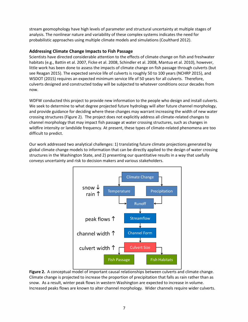
Addressing Climate Change Impacts to Fish Passage Scientists have directed considerable attention to the effects of climate change on fish and freshwater habitats (e.g., Battin et al. 2007, Ficke et al. 2008, Schindler et al. 2008, Mantua et al. 2010), however, little work has been done to assess the impacts of climate change on fish passage through culverts (but see Reagan 2015). The expected service life of culverts is roughly 50 to 100 years (NCHRP 2015), and WSDOT (2015) requires an expected minimum service life of 50 years for all culverts. Therefore, culverts designed and constructed today will be subjected to whatever conditions occur decades from now. WDFW conducted this project to provide new information to the people who design and install culverts. We seek to determine to what degree projected future hydrology will alter future channel morphology, and provide guidance for deciding where these changes may warrant increasing the width of new water crossing structures (Figure 2). The project does not explicitly address all climate-related changes to channel morphology that may impact fish passage at water crossing structures, such as changes in wildfire intensity or landslide frequency. At present, these types of climate-related phenomena are too difficult to predict. Our work addressed two analytical challenges: 1) translating future climate projections generated by global climate change models to information that can be directly applied to the design of water crossing structures in the Washington State, and 2) presenting our quantitative results in a way that usefully conveys uncertainty and risk to decision makers and various stakeholders.

Figure 2. A conceptual model of important causal relationships between culverts and climate change. Climate change is projected to increase the proportion of precipitation that falls as rain rather than as snow. As a result, winter peak flows in western Washington are expected to increase in volume. Increased peaks flows are known to alter channel morphology. Wider channels require wider culverts.

8

2. Methods − Projecting Future Bankfull Flows and Bankfull Widths

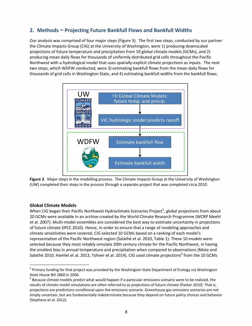
Our analysis was comprised of four major steps (Figure 3). The first two steps, conducted by our partner the Climate Impacts Group (CIG) at the University of Washington, were 1) producing downscaled projections of future temperature and precipitation from 10 global climate models (GCMs), and 2) producing mean daily flows for thousands of uniformly distributed grid cells throughout the Pacific Northwest with a hydrological model that uses spatially-explicit climate projections as inputs. The next two steps, which WDFW conducted, were 3) estimating bankfull flows from the mean daily flows for thousands of grid cells in Washington State, and 4) estimating bankfull widths from the bankfull flows.

Figure 3. Major steps in the modelling process. The Climate Impacts Group at the University of Washington (UW) completed their steps in the process through a separate project that was completed circa 2010.

Global Climate Models When CIG began their Pacific Northwest Hydroclimate Scenarios Project5, global projections from about 20 GCMs were available in an archive created by the World Climate Research Programme (WCRP Meehl et al. 2007). Multi-model ensembles are considered the best way to estimate uncertainty in projections of future climate (IPCC 2010). Hence, In order to ensure that a range of modeling approaches and climate sensitivities were covered, CIG selected 10 GCMs based on a ranking of each model’s representation of the Pacific Northwest region (Salathé et al. 2010, Table 1). These 10 models were selected because they most reliably simulate 20th century climate for the Pacific Northwest, in having the smallest bias in annual temperature and precipitation when compared to observations (Mote and Salathè 2010, Hamlet et al. 2013, Tohver et al. 2014). CIG used climate projections6 from the 10 GCMs

5 Primary funding for that project was provided by the Washington State Department of Ecology via Washington

State House Bill 2860 in 2006. 6 Because climate models predict what would happen if a particular emissions scenario were to be realized, the

results of climate model simulations are often referred to as projections of future climate (Parker 2010). That is, projections are predictions conditional upon the emissions scenario. Greenhouse gas emissions scenarios are not simply uncertain, but are fundamentally indeterminate because they depend on future policy choices and behavior (Stephens et al. 2012).

9

under the A1B greenhouse gas scenario, a moderate scenario that assumes “business as usual” emissions through the first half of the 21st century followed by substantial mitigation measures after 2050 (Nakicenovic et al. 2000, Figure 4). Climate projections were generated for two future 30-year time periods, intended to be representative of the statistics of the middle decade of each time period: 2030-2059 (referred to as the “2040s”) and 2070-2099 (“2080s”). GCMs are generally run at a spatial resolution of 100 to 300 km (Randall et al. 2007). CIG downscaled the projections from each of the 10 GCMs to 1/16-degree latitude x 1/16-degree longitude grid cells (≈ 5 x 7 km or ≈33 km2/cell), which divides Washington State into 5,270 grid cells. Downscaling requires a reference historical dataset. An observationally-based historical data set for daily precipitation, maximum and minimum daily temperature, and wind speed was developed at 1/16-degree spatial resolution for the years 1915 to 2006. CIG used the National Climatic Data Center Cooperative Observer network and Environment Canada daily station data as the primary sources for precipitation and temperature values (Elsner et al. 2010). Daily wind speed values for 1949–2006 were downscaled from National Centers for Environmental Prediction-National Center for Atmospheric Research reanalysis products (Kalanay et al. 1996). For years prior to 1949, a daily wind speed climatology was derived from the same 1949–2006 reanalysis. Downscaling was done with the hybrid delta method (Salathè et al 2007, Hamlet et al. 2010), which CIG developed specifically for the Pacific Northwest Hydroclimate Scenarios Project. It is designed to combine the most robust aspects of GCM projections (specifically, changes in the monthly probability distribution of temperature and precipitation) with the observed features of regional daily weather patterns (Hamlet et al. 2013). Global model projections are first bias-corrected to match historical observations; this is applied at the original coarse spatial resolution of each GCM. The bias-corrected GCM projections are then spatially interpolated to the 1/16-degree resolution. The monthly downscaling is completed by applying the model-projected change in the probability distributions of temperature and precipitation to each month in the historical record (1915-2006). Finally, this monthly time series is disaggregated to the daily time series needed for extremes analyses by applying each GCM's projected monthly change to the observed daily values separately for each grid cell (Tohver et al. 2014).

10

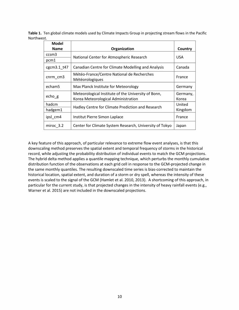
Table 1. Ten global climate models used by Climate Impacts Group in projecting stream flows in the Pacific Northwest.

Model Name Organization Country

ccsm3 National Center for Atmospheric Research USA

pcm1

cgcm3.1_t47 Canadian Centre for Climate Modelling and Analysis Canada

cnrm_cm3 Météo-France/Centre National de Recherches Météorologiques

France

echam5 Max Planck Institute for Meteorology Germany

echo_g Meteorological Institute of the University of Bonn, Korea Meteorological Administration

Germany, Korea

hadcm Hadley Centre for Climate Prediction and Research

United Kingdom hadgem1

ipsl_cm4 Institut Pierre Simon Laplace France

miroc_3.2 Center for Climate System Research, University of Tokyo Japan

A key feature of this approach, of particular relevance to extreme flow event analyses, is that this downscaling method preserves the spatial extent and temporal frequency of storms in the historical record, while adjusting the probability distribution of individual events to match the GCM projections. The hybrid delta method applies a quantile mapping technique, which perturbs the monthly cumulative distribution function of the observations at each grid cell in response to the GCM-projected change in the same monthly quantiles. The resulting downscaled time series is bias-corrected to maintain the historical location, spatial extent, and duration of a storm or dry spell, whereas the intensity of these events is scaled to the signal of the GCM (Hamlet et al. 2010, 2013). A shortcoming of this approach, in particular for the current study, is that projected changes in the intensity of heavy rainfall events (e.g., Warner et al. 2015) are not included in the downscaled projections.

11

A B

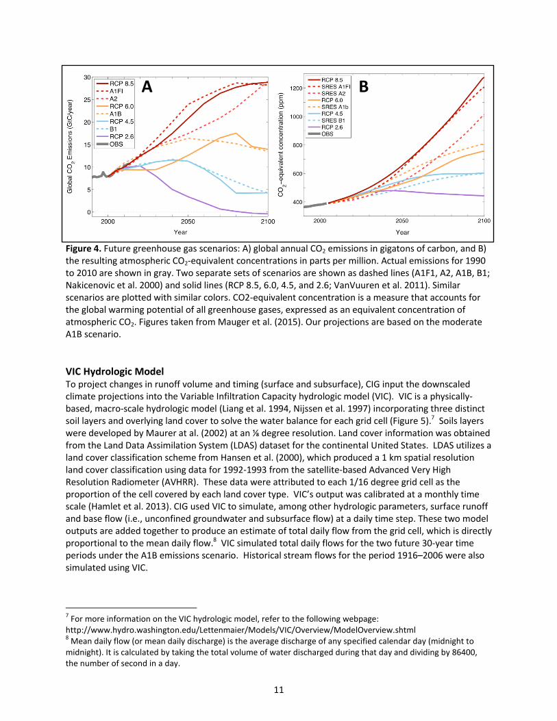
Figure 4. Future greenhouse gas scenarios: A) global annual CO2 emissions in gigatons of carbon, and B) the resulting atmospheric CO2-equivalent concentrations in parts per million. Actual emissions for 1990 to 2010 are shown in gray. Two separate sets of scenarios are shown as dashed lines (A1F1, A2, A1B, B1; Nakicenovic et al. 2000) and solid lines (RCP 8.5, 6.0, 4.5, and 2.6; VanVuuren et al. 2011). Similar scenarios are plotted with similar colors. CO2-equivalent concentration is a measure that accounts for the global warming potential of all greenhouse gases, expressed as an equivalent concentration of atmospheric CO2. Figures taken from Mauger et al. (2015). Our projections are based on the moderate A1B scenario.

VIC Hydrologic Model To project changes in runoff volume and timing (surface and subsurface), CIG input the downscaled climate projections into the Variable Infiltration Capacity hydrologic model (VIC). VIC is a physically-based, macro-scale hydrologic model (Liang et al. 1994, Nijssen et al. 1997) incorporating three distinct soil layers and overlying land cover to solve the water balance for each grid cell (Figure 5).7 Soils layers were developed by Maurer at al. (2002) at an ⅛ degree resolution. Land cover information was obtained from the Land Data Assimilation System (LDAS) dataset for the continental United States. LDAS utilizes a land cover classification scheme from Hansen et al. (2000), which produced a 1 km spatial resolution land cover classification using data for 1992-1993 from the satellite-based Advanced Very High Resolution Radiometer (AVHRR). These data were attributed to each 1/16 degree grid cell as the proportion of the cell covered by each land cover type. VIC’s output was calibrated at a monthly time scale (Hamlet et al. 2013). CIG used VIC to simulate, among other hydrologic parameters, surface runoff and base flow (i.e., unconfined groundwater and subsurface flow) at a daily time step. These two model outputs are added together to produce an estimate of total daily flow from the grid cell, which is directly proportional to the mean daily flow.8 VIC simulated total daily flows for the two future 30-year time periods under the A1B emissions scenario. Historical stream flows for the period 1916–2006 were also simulated using VIC.

7 For more information on the VIC hydrologic model, refer to the following webpage:

http://www.hydro.washington.edu/Lettenmaier/Models/VIC/Overview/ModelOverview.shtml 8 Mean daily flow (or mean daily discharge) is the average discharge of any specified calendar day (midnight to

midnight). It is calculated by taking the total volume of water discharged during that day and dividing by 86400, the number of second in a day.

12

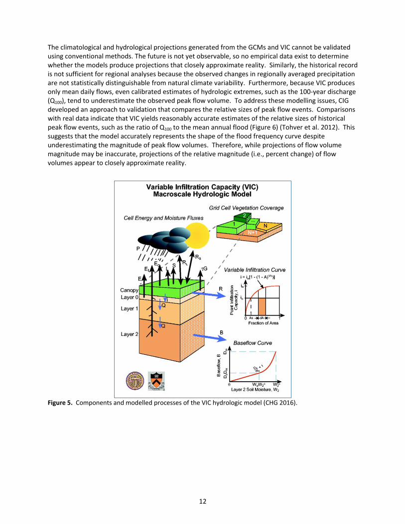
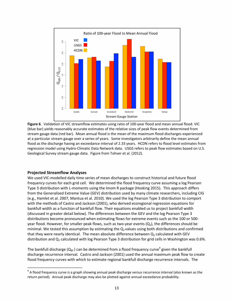
The climatological and hydrological projections generated from the GCMs and VIC cannot be validated using conventional methods. The future is not yet observable, so no empirical data exist to determine whether the models produce projections that closely approximate reality. Similarly, the historical record is not sufficient for regional analyses because the observed changes in regionally averaged precipitation are not statistically distinguishable from natural climate variability. Furthermore, because VIC produces only mean daily flows, even calibrated estimates of hydrologic extremes, such as the 100-year discharge (Q100), tend to underestimate the observed peak flow volume. To address these modelling issues, CIG developed an approach to validation that compares the relative sizes of peak flow events. Comparisons with real data indicate that VIC yields reasonably accurate estimates of the relative sizes of historical peak flow events, such as the ratio of Q100 to the mean annual flood (Figure 6) (Tohver et al. 2012). This suggests that the model accurately represents the shape of the flood frequency curve despite underestimating the magnitude of peak flow volumes. Therefore, while projections of flow volume magnitude may be inaccurate, projections of the relative magnitude (i.e., percent change) of flow volumes appear to closely approximate reality. Figure 5. Components and modelled processes of the VIC hydrologic model (CHG 2016).

13

Figure 6. Validation of VIC streamflow estimates using ratio of 100-year flood and mean annual flood. VIC (blue bar) yields reasonably accurate estimates of the relative sizes of peak flow events determined from stream gauge data (red bar). Mean annual flood is the mean of the maximum flood discharges experienced at a particular stream gauge over a series of years. Some investigators arbitrarily define the mean annual flood as the discharge having an exceedance interval of 2.33 years. HCDN refers to flood level estimates from regression model using Hydro-Climatic Data Network data. USGS refers to peak flow estimates based on U.S. Geological Survey stream gauge data. Figure from Tohver et al. (2012).

Projected Streamflow Analyses We used VIC-modelled daily time series of mean discharges to construct historical and future flood frequency curves for each grid cell. We determined the flood frequency curve assuming a log Pearson Type 3 distribution with L-moments using the lmom R package (Hosking 2015). This approach differs from the Generalized Extreme Value (GEV) distribution used by many climate researchers, including CIG (e.g., Hamlet et al. 2007, Mantua et al. 2010). We used the log Pearson Type 3 distribution to comport with the methods of Castro and Jackson (2001), who derived ecoregional regression equations for bankfull width as a function of bankfull flow. Their equations enabled us to project bankfull width (discussed in greater detail below). The differences between the GEV and the log Pearson Type 3 distributions become pronounced when estimating flows for extreme events such as the 100 or 500-year flood. However, for smaller peak flows, such as two-year events (Q2), the differences should be minimal. We tested this assumption by estimating the Q2 values using both distributions and confirmed that they were nearly identical. The mean absolute difference between Q2 calculated with GEV distribution and Q2 calculated with log Pearson Type 3 distribution for grid cells in Washington was 0.6%. The bankfull discharge (QBF ) can be determined from a flood frequency curve9 given the bankfull discharge recurrence interval. Castro and Jackson (2001) used the annual maximum peak flow to create flood frequency curves with which to estimate regional bankfull discharge recurrence intervals. The

9 A flood frequency curve is a graph showing annual peak discharge versus recurrence interval (also known as the

return period). Annual peak discharge may also be plotted against annual exceedance probability.

14

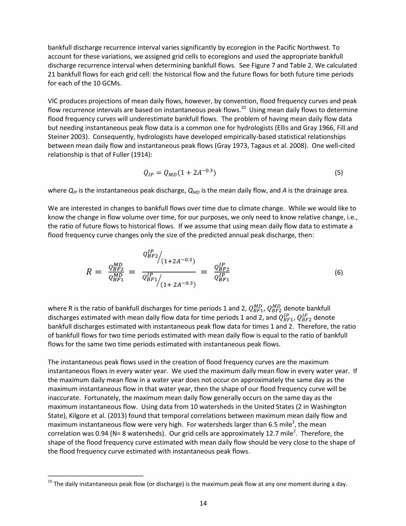
bankfull discharge recurrence interval varies significantly by ecoregion in the Pacific Northwest. To account for these variations, we assigned grid cells to ecoregions and used the appropriate bankfull discharge recurrence interval when determining bankfull flows. See Figure 7 and Table 2. We calculated 21 bankfull flows for each grid cell: the historical flow and the future flows for both future time periods for each of the 10 GCMs. VIC produces projections of mean daily flows, however, by convention, flood frequency curves and peak flow recurrence intervals are based on instantaneous peak flows.10 Using mean daily flows to determine flood frequency curves will underestimate bankfull flows. The problem of having mean daily flow data but needing instantaneous peak flow data is a common one for hydrologists (Ellis and Gray 1966, Fill and Steiner 2003). Consequently, hydrologists have developed empirically-based statistical relationships between mean daily flow and instantaneous peak flows (Gray 1973, Tagaus et al. 2008). One well-cited relationship is that of Fuller (1914):

𝑄𝐼𝑃 = 𝑄𝑀𝐷(1 + 2𝐴−0.3) (5) where QIP is the instantaneous peak discharge, QMD is the mean daily flow, and A is the drainage area. We are interested in changes to bankfull flows over time due to climate change. While we would like to know the change in flow volume over time, for our purposes, we only need to know relative change, i.e., the ratio of future flows to historical flows. If we assume that using mean daily flow data to estimate a flood frequency curve changes only the size of the predicted annual peak discharge, then:

𝑅 = 𝑄𝐵𝐹2

𝑀𝐷

𝑄𝐵𝐹1𝑀𝐷 =

𝑄𝐵𝐹2𝐼𝑃

(1+2𝐴−0.3)⁄

𝑄𝐵𝐹1𝐼𝑃

(1+ 2𝐴−0.3)⁄

= 𝑄𝐵𝐹2

𝐼𝑃

𝑄𝐵𝐹1𝐼𝑃 (6)

where R is the ratio of bankfull discharges for time periods 1 and 2, 𝑄𝐵𝐹1𝑀𝐷 , 𝑄𝐵𝐹2

𝑀𝐷 denote bankfull

discharges estimated with mean daily flow data for time periods 1 and 2, and 𝑄𝐵𝐹1𝐼𝑃 , 𝑄𝐵𝐹2

𝐼𝑃 denote bankfull discharges estimated with instantaneous peak flow data for times 1 and 2. Therefore, the ratio of bankfull flows for two time periods estimated with mean daily flow is equal to the ratio of bankfull flows for the same two time periods estimated with instantaneous peak flows. The instantaneous peak flows used in the creation of flood frequency curves are the maximum instantaneous flows in every water year. We used the maximum daily mean flow in every water year. If the maximum daily mean flow in a water year does not occur on approximately the same day as the maximum instantaneous flow in that water year, then the shape of our flood frequency curve will be inaccurate. Fortunately, the maximum mean daily flow generally occurs on the same day as the maximum instantaneous flow. Using data from 10 watersheds in the United States (2 in Washington State), Kilgore et al. (2013) found that temporal correlations between maximum mean daily flow and maximum instantaneous flow were very high. For watersheds larger than 6.5 mile2, the mean correlation was 0.94 (N= 8 watersheds). Our grid cells are approximately 12.7 mile2. Therefore, the shape of the flood frequency curve estimated with mean daily flow should be very close to the shape of the flood frequency curve estimated with instantaneous peak flows.

10

The daily instantaneous peak flow (or discharge) is the maximum peak flow at any one moment during a day.

15

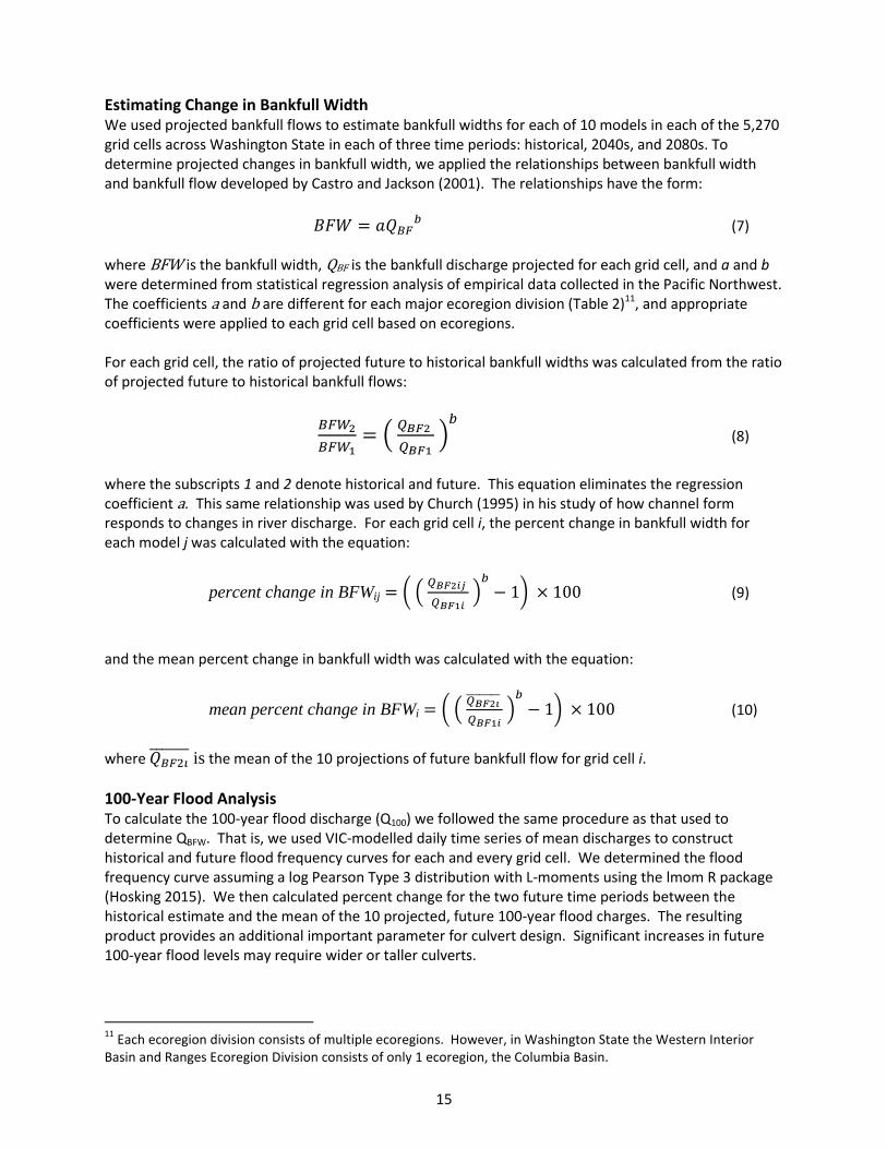
Estimating Change in Bankfull Width We used projected bankfull flows to estimate bankfull widths for each of 10 models in each of the 5,270 grid cells across Washington State in each of three time periods: historical, 2040s, and 2080s. To determine projected changes in bankfull width, we applied the relationships between bankfull width and bankfull flow developed by Castro and Jackson (2001). The relationships have the form:

𝐵𝐹𝑊 = 𝑎𝑄𝐵𝐹𝑏 (7)

where BFW is the bankfull width, QBF is the bankfull discharge projected for each grid cell, and a and b were determined from statistical regression analysis of empirical data collected in the Pacific Northwest. The coefficients a and b are different for each major ecoregion division (Table 2)11, and appropriate coefficients were applied to each grid cell based on ecoregions. For each grid cell, the ratio of projected future to historical bankfull widths was calculated from the ratio of projected future to historical bankfull flows:

𝐵𝐹𝑊2

𝐵𝐹𝑊1= (

𝑄𝐵𝐹2

𝑄𝐵𝐹1 )

𝑏 (8)

where the subscripts 1 and 2 denote historical and future. This equation eliminates the regression coefficient a. This same relationship was used by Church (1995) in his study of how channel form responds to changes in river discharge. For each grid cell i, the percent change in bankfull width for each model j was calculated with the equation:

percent change in BFWij = ( ( 𝑄𝐵𝐹2𝑖𝑗

𝑄𝐵𝐹1𝑖 )

𝑏

− 1) × 100 (9)

and the mean percent change in bankfull width was calculated with the equation:

mean percent change in BFWi = ( ( 𝑄𝐵𝐹2𝑖̅̅ ̅̅ ̅̅ ̅̅

𝑄𝐵𝐹1𝑖 )

𝑏

− 1) × 100 (10)

where 𝑄𝐵𝐹2𝑖̅̅ ̅̅ ̅̅ ̅ is the mean of the 10 projections of future bankfull flow for grid cell i.

100-Year Flood Analysis To calculate the 100-year flood discharge (Q100) we followed the same procedure as that used to determine QBFW. That is, we used VIC-modelled daily time series of mean discharges to construct historical and future flood frequency curves for each and every grid cell. We determined the flood frequency curve assuming a log Pearson Type 3 distribution with L-moments using the lmom R package (Hosking 2015). We then calculated percent change for the two future time periods between the historical estimate and the mean of the 10 projected, future 100-year flood charges. The resulting product provides an additional important parameter for culvert design. Significant increases in future 100-year flood levels may require wider or taller culverts.

11

Each ecoregion division consists of multiple ecoregions. However, in Washington State the Western Interior Basin and Ranges Ecoregion Division consists of only 1 ecoregion, the Columbia Basin.

16

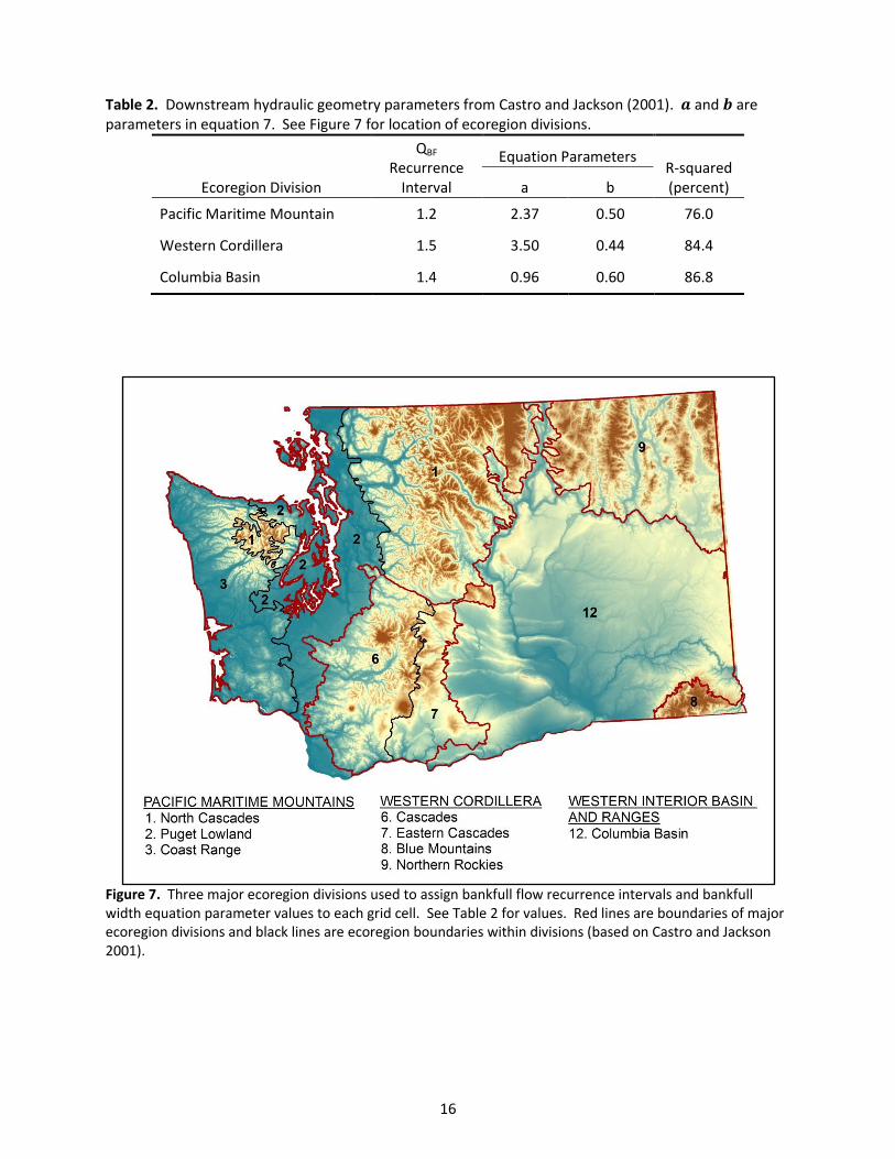
Table 2. Downstream hydraulic geometry parameters from Castro and Jackson (2001). 𝒂 and 𝒃 are parameters in equation 7. See Figure 7 for location of ecoregion divisions.

Ecoregion Division

QBF Recurrence

Interval

Equation Parameters R-squared (percent) a b

Pacific Maritime Mountain 1.2 2.37 0.50 76.0

Western Cordillera 1.5 3.50 0.44 84.4

Columbia Basin 1.4 0.96 0.60 86.8

Figure 7. Three major ecoregion divisions used to assign bankfull flow recurrence intervals and bankfull width equation parameter values to each grid cell. See Table 2 for values. Red lines are boundaries of major ecoregion divisions and black lines are ecoregion boundaries within divisions (based on Castro and Jackson 2001).

17

3. Results

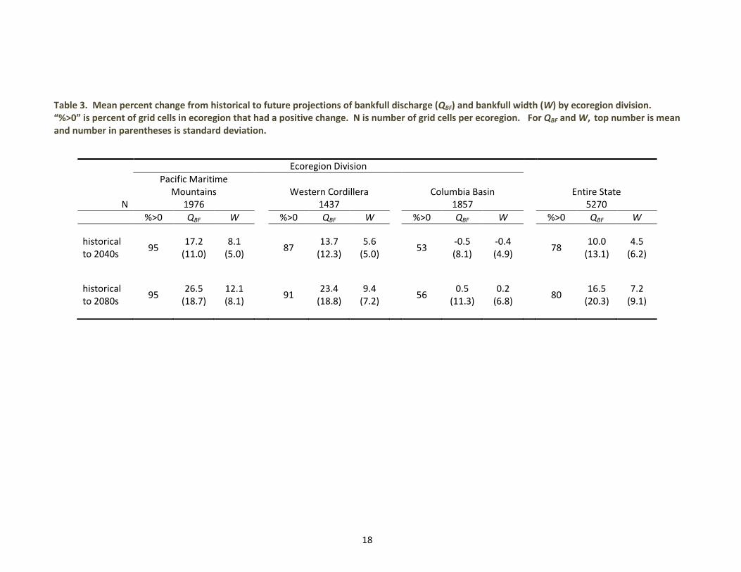
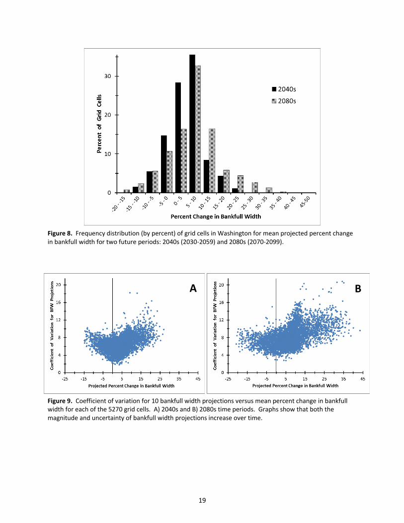
Projected Changes in Bankfull Width In both future time periods, about 80% of grid cells in Washington are projected to have an increase in bankfull discharge and a consequent increase in BFW (Table 3). Mean percent change in BFW increased over time. The mean for the 5,270 grid cells of mean percent change in bankfull width was 4.5 and 7.2% for the 2040s and 2080s time periods, respectively. In the 2040s, nearly half (49.8%) had a mean percent change in BFW greater that 5%, and 14% of grid cells had a change greater than 10% (Figure 8). In the 2080s, roughly two-thirds (64%) of grid cells had a mean percent change in BFW greater that 5%, and almost one-third (31%) had a change greater than 10%. The maximum mean percent change in BFW was 27.0% in the 2040s and 43.5% in the 2080s; both occur in the North Cascades Ecoregion. Mean percent change in bankfull discharge and consequent mean percent change in bankfull width varied by ecoregion (Table 3, Figure 10). For the Pacific Maritime Mountain Ecoregion Division in the 2080s, the average of mean percent change in bankfull width was 12.1 but almost zero (0.2) for the Columbia Basin. Furthermore, in the Pacific Maritime Mountain Ecoregion, 95% of grid cells are projected to exhibit wider bankfull widths in the 2080s, but in the Columbia Basin only 56% of cells are projected to exhibit an increase. Seventy-seven percent of grid cells with projected negative change in BFW in the 2080s occurred in the Columbia Basin. Mean percent changes in bankfull width varied by elevation, with the largest changes occurring in high elevation grid cells that have mixed rain-on-snow and snow dominated hydrographs. Consequently, the largest increases in mean percent change in bankfull width occurred in the most mountainous ecoregion, the North Cascades. The largest decreases in percent change in BFW occurred in the Columbia Basin. Variation amongst the 10 BFW projections for each grid cell, as expressed by the coefficient of variation (CV), was remarkably low. The median and maximum CVs for projected future BFW among 10 models across all grid cells was 6.4 and 16.1% for the 2040s and 8.1 and 20.7% for the 2080s (Figure 9). This indicates a high level of agreement amongst BFW projections. However, variability (i.e., disagreement amongst models) in projected BFW increases as the magnitude of mean percent change in BFW increases. This is especially evident in the 2080s time period. Model projections within a grid cell can range from negative change to positive change. In fact, in the 2080s, 70% of grid cells had some disagreement amongst models about the direction of change in BFW. However, 75% of grid cells had at least a moderate level of agreement amongst models (i.e., 7 to 10 models) on the direction of change. Furthermore, 30.1% of grid cells had consensus amongst all 10 models for the direction of change: 27.7% of grid cells had all 10 models project an increase and 2.4% of grid cells had all 10 models project a decrease.

18

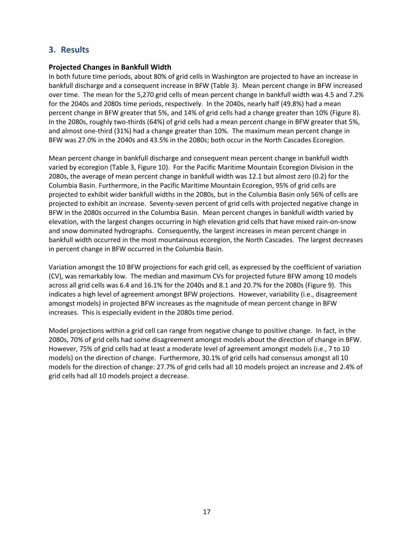
Table 3. Mean percent change from historical to future projections of bankfull discharge (QBF) and bankfull width (W) by ecoregion division. “%>0” is percent of grid cells in ecoregion that had a positive change. N is number of grid cells per ecoregion. For QBF and W, top number is mean and number in parentheses is standard deviation.

Ecoregion Division

Pacific Maritime Mountains

Western Cordillera

Columbia Basin

Entire State

N 1976 1437 1857 5270

%>0 QBF W %>0 QBF W %>0 QBF W %>0 QBF W

historical to 2040s

95 17.2

(11.0) 8.1

(5.0)

87 13.7

(12.3) 5.6

(5.0)

53 -0.5 (8.1)

-0.4 (4.9)

78 10.0

(13.1) 4.5

(6.2)

historical to 2080s

95 26.5

(18.7) 12.1 (8.1)

91 23.4

(18.8) 9.4

(7.2)

56 0.5

(11.3) 0.2

(6.8)

80 16.5

(20.3) 7.2

(9.1)

19

A

Figure 8. Frequency distribution (by percent) of grid cells in Washington for mean projected percent change in bankfull width for two future periods: 2040s (2030-2059) and 2080s (2070-2099).

Figure 9. Coefficient of variation for 10 bankfull width projections versus mean percent change in bankfull width for each of the 5270 grid cells. A) 2040s and B) 2080s time periods. Graphs show that both the magnitude and uncertainty of bankfull width projections increase over time.

B

20

Figure 10. The mean (of 10 models) projected percent change in bankfull width for the A) 2040s and B) 2080s time periods. Black lines are ecoregion boundaries. Grid cells are 1/16-degree latitude x 1/16-degree longitude (approximately 5 x 7 km).

A

B

21

A

B

z

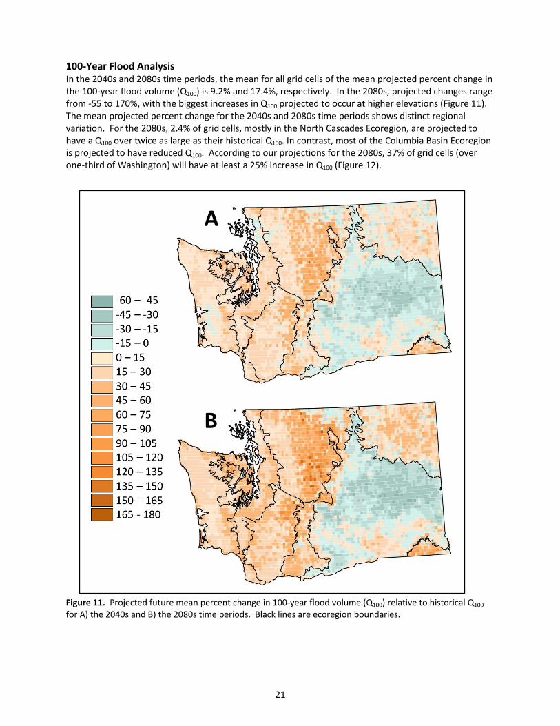
100-Year Flood Analysis In the 2040s and 2080s time periods, the mean for all grid cells of the mean projected percent change in the 100-year flood volume (Q100) is 9.2% and 17.4%, respectively. In the 2080s, projected changes range from -55 to 170%, with the biggest increases in Q100 projected to occur at higher elevations (Figure 11). The mean projected percent change for the 2040s and 2080s time periods shows distinct regional variation. For the 2080s, 2.4% of grid cells, mostly in the North Cascades Ecoregion, are projected to have a Q100 over twice as large as their historical Q100. In contrast, most of the Columbia Basin Ecoregion is projected to have reduced Q100. According to our projections for the 2080s, 37% of grid cells (over one-third of Washington) will have at least a 25% increase in Q100 (Figure 12).

Figure 11. Projected future mean percent change in 100-year flood volume (Q100) relative to historical Q100 for A) the 2040s and B) the 2080s time periods. Black lines are ecoregion boundaries.

22

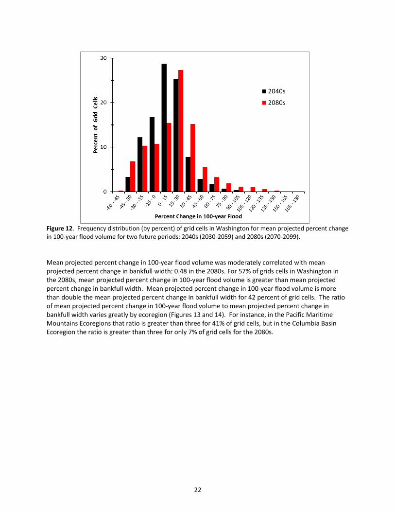
Figure 12. Frequency distribution (by percent) of grid cells in Washington for mean projected percent change in 100-year flood volume for two future periods: 2040s (2030-2059) and 2080s (2070-2099).

Mean projected percent change in 100-year flood volume was moderately correlated with mean projected percent change in bankfull width: 0.48 in the 2080s. For 57% of grids cells in Washington in the 2080s, mean projected percent change in 100-year flood volume is greater than mean projected percent change in bankfull width. Mean projected percent change in 100-year flood volume is more than double the mean projected percent change in bankfull width for 42 percent of grid cells. The ratio of mean projected percent change in 100-year flood volume to mean projected percent change in bankfull width varies greatly by ecoregion (Figures 13 and 14). For instance, in the Pacific Maritime Mountains Ecoregions that ratio is greater than three for 41% of grid cells, but in the Columbia Basin Ecoregion the ratio is greater than three for only 7% of grid cells for the 2080s.

23

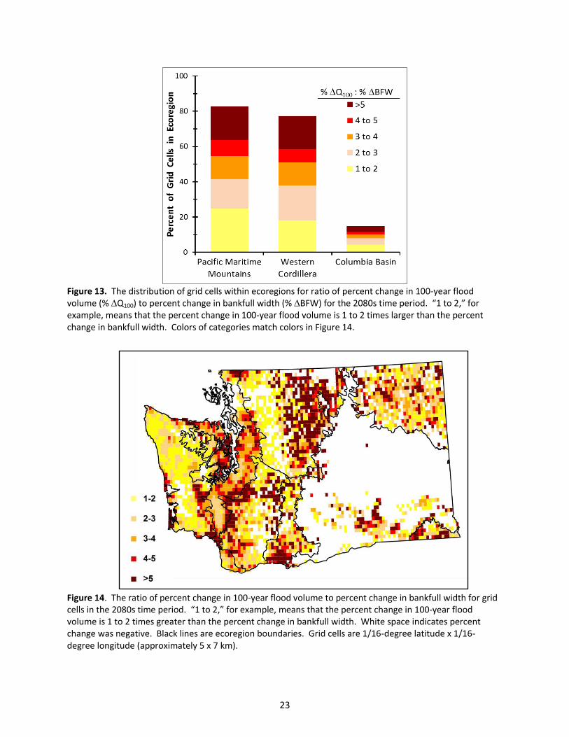
Figure 13. The distribution of grid cells within ecoregions for ratio of percent change in 100-year flood volume (% ∆Q100) to percent change in bankfull width (% ∆BFW) for the 2080s time period. “1 to 2,” for example, means that the percent change in 100-year flood volume is 1 to 2 times larger than the percent change in bankfull width. Colors of categories match colors in Figure 14.

Figure 14. The ratio of percent change in 100-year flood volume to percent change in bankfull width for grid cells in the 2080s time period. “1 to 2,” for example, means that the percent change in 100-year flood volume is 1 to 2 times greater than the percent change in bankfull width. White space indicates percent change was negative. Black lines are ecoregion boundaries. Grid cells are 1/16-degree latitude x 1/16-degree longitude (approximately 5 x 7 km).

24

4. Information for Culvert Design

Based on current engineering standards, culverts are expected to last 50 to 100 years (NCHRP 2015, WSDOT 2015). If culverts installed today do not accommodate increases in bankfull width caused by future increases in bankfull flow, then undersized culverts could create fish passage barriers and damage fish habitats, require increased maintenance and repairs, or undergo catastrophic structural failure during floods. A fiscally responsible approach to incorporating climate change projections into culvert design must weigh the trade-off between the certain costs of a wider culvert now, which accommodates projected changes in bankfull width versus the uncertain future costs of damages to natural resources and public infrastructure that could occur if projected future changes are not adequately accommodated. Because the decision to build or not to build wider culverts leads to an uncertain outcome with potentially adverse consequences, that decision involves risk. Decision makers should address this risk, and our analysis can serve as the basis for a simple risk assessment that informs decisions regarding culvert design.

Uncertainty All assessments in natural resources management, and the models they depend upon, are uncertain. Our assessment has three main sources of uncertainty, which correspond to the major steps of our assessment: 1) global climate models, 2) the hydrologic model and bankfull flow projections, and 3) bankfull width estimates using hydraulic geometry relationships. We addressed each source of uncertainty as follows. Relationships between stream discharge and channel geometry are very well understood (Singh 2003, Buffington 2012, Gleason 2015), and the empirical relationships we utilized (Castro and Jackson 2001) have high coefficients of determination (r2). Statistical regressions using data from three ecoregions produced r2 equal to 0.76, 0.84, and 0.87, which are very good fits to the data and perhaps as good as one could hope for in a study of natural systems. Furthermore, equation 8 for calculation of future to historical bankfull width ratios eliminated the regression coefficient a. Regression coefficients are parameter estimates with some uncertainty (i.e., a standard error). Hence, by eliminating one of the regression coefficients, we reduced uncertainty in our predictions based on hydraulic geometry. Therefore, while application of the hydraulic geometry relationships will result in some error, we believe that the error is small enough to be ignored for our purposes.

VIC is a model, and no model can generate error-free predictions. Furthermore, because VIC produces mean daily flows, it underestimates peak flow volumes. Despite these shortcomings, comparisons done by CIG indicate that VIC yields reasonably accurate estimates of the relative sizes of historical peak flow events, such as the ratio of Q100 to the mean annual flood (Tohver et al. 2012). Therefore, for the purposes of culvert design, we believe the error in the ratio of bankfull flow estimates (equation 8) is small enough to be ignored for our purposes.

The greatest uncertainty lies in the climate change projections. CIG used an ensemble of 10 GCMs to ensure that a range of modeling approaches and climate sensitivities were included. This ensemble was drawn from the larger pool of available GCMs based on an assessment of each model’s ability to capture key characteristics of the Pacific Northwest Region’s historical climate (Salathè et al. 2007, Mote and Salathè 2010). Multi-model averages for a variety of climate variables generally agree better with observations of present day climate than any single model (Knutti et al. 2010, IPCC 2010), and unweighted multi-model averages are often presented as “best guess” projections (Tebaldi and Knutti 2007). Multi-model ensembles have become standard practice for dealing with uncertainty in climate change projections (IPCC 2010), and more “robust” projections are those with more agreement amongst models within an ensemble (Parker 2013). Hence, we used CIG’s 10-model ensemble to describe uncertainty in future changes in bankfull width.

25

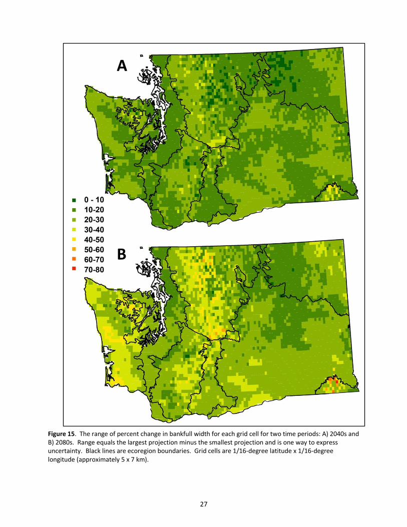
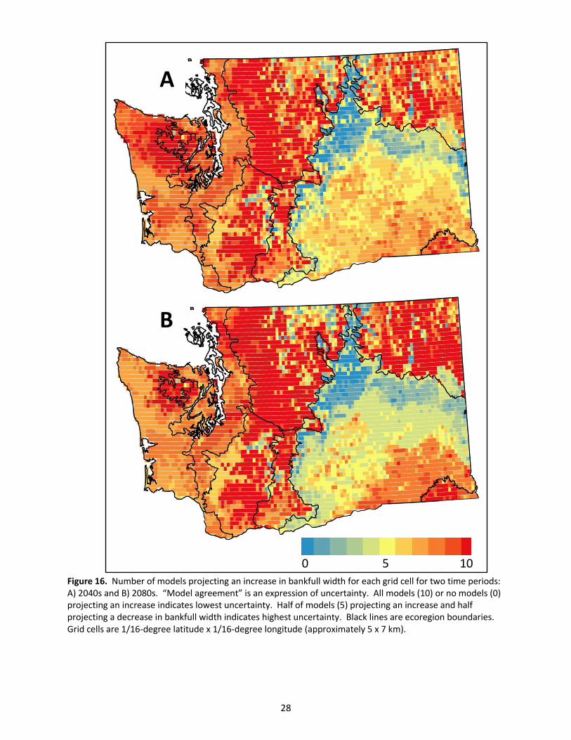
Because a multi-model ensemble is neither a random nor a systematic sample of GCMs, it is unclear how to interpret the uncertainty conveyed by an ensemble (Knutti 2010). Hence, the most credible ways to communicate uncertainty are often the simplest (Kandlikar et al. 2005). The range of projections (i.e., maximum minus minimum) for percent change in bankfull width produced by the 10 models is perhaps the simplest expression of uncertainty. Based on the range of projections, the greatest uncertainty in future changes in bankfull width occur in the higher elevations of the Olympic Mountains, the northern portion of the Cascade Mountains, and the Blue Mountains in southeast Washington (Figure 15A). As expected, the range of projections farther in the future becomes wider, i.e., more uncertain (Figure 15B). Another simple measure of uncertainty is the number of models that agree on the sign of change (Kandlikar et al. 2005, Tebaldi et al. 2011). We have the lowest uncertainty when all models or zero models project a positive change (i.e., an increase) in bankfull width. Half the models projecting a positive change and half projecting a negative change in bankfull width indicates highest uncertainty. In Washington, the highest model agreement occurs in mountainous regions – the Olympics, Cascades, Blues, and the Selkirks in northeastern Washington – where all models project a positive change in some grid cells, and along the margins of the Columbia Basin Ecoregion where all the models project a negative change in some grid cells (Figure 16). Throughout most of Washington model agreement does not change substantially between time periods, with the exceptions of southeastern Washington where model agreement increases, and the plains and foothills of the Coast Range Ecoregion where model agreement decreases.

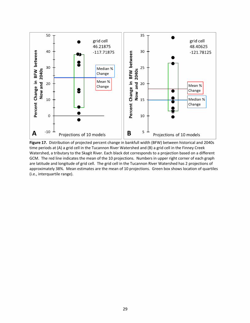
Because quantitative expressions of uncertainty are problematic for multi-model ensembles, we developed a graphical depiction of uncertainty. The graph simply shows the distribution of values projected by the 10 models along with the mean. In one example (Figure 17A), the distribution of future percent changes in bankfull width has a range of 48%, the distribution is evenly distributed around the mean with five projections above the mean and five below, and the mean (22.2%) lies roughly in the middle of the distribution (located at 21.7%). The wide range and relatively uniform distribution of values within that range indicate a lot of uncertainty regarding percent change in bankfull width for this grid cell. On the other hand, nine of ten models project an increase in bankfull width, and therefore, we can feel confident that an increase will occur between now and the 2040s.

In another example (Figure 17B), the distribution of future percent changes in bankfull width has a range of 25%, and the distribution is unevenly distributed around the mean, with three projections above the mean and seven below. The density of points between 9 and 18 percent shows relatively close agreement for 7 of 10 models. However, three models project an increase of at least 26%. The mean percent change is 18%, but this skewed distribution indicates the possibility, however unlikely, of more extremes increases in bankfull width. In this example, all ten models project an increase in bankfull width. Graphs such as these can help managers and engineers think about the chance that bankfull width at a particular location will increase over time due to climate change.

Risk and Actionable Risk Risk is a measure of the chance and the consequence of an uncertain future event (Yoe 2012, p. 1). Risk consists of two parts: an undesirable outcome and the probability of that outcome occurring. A common formula for risk is (Modarres et al. 1999, p. 466):

𝑅𝑖𝑠𝑘 = 𝑃𝑟𝑜𝑏𝑎𝑏𝑖𝑙𝑖𝑡𝑦 × 𝐶𝑜𝑠𝑡 (11)

Probability is one way to express uncertainty, and “cost” is a synonym for the potential amount of damage, harm, loss of value, or lost opportunity. Whenever uncertainty and “cost” coincide there is risk. Decisions about culvert design entail uncertainty about future changes to channel form and “cost” arising from potential future damages to fish habitats and public infrastructure.

26

When making decisions, managers should consider all risks, but actually eliminating or minimizing all risks may be impractical. Therefore, managers must decide which risks are “actionable.” An actionable risk has three characteristics: 1) it is described by information that is specific, unbiased, credible and usable (IGES 2012); 2) the risk exceeds the manager’s risk tolerance, and consequently, it gives cause or a reason for action; and 3) the risk can be acted upon, i.e., actions can be taken to eliminate or minimize the risk. We believe we have produced information that is actionable, i.e., based on the best available science that is specific to culvert design, unbiased, and credible. We have also created a graphical depiction of risk that makes our information useable for managers (Figure 18). Risk has two components: probability and cost. We lack estimates for both components; however, our bankfull width projections provide useful surrogates. Our surrogate for probability is our simple measure of uncertainty − the proportion or number of models that agree on the sign of change. Our surrogate for cost is the relative amount of undersizing. If a culvert built using today’s bankfull width is too narrow to accommodate future bankfull width, then we expect that culvert to become an impediment to fish passage. That is, as the disparity between channel width and culvert width increases, we expect the culvert’s capacity to pass fish to decrease. In other words, the channel-culvert width disparity and fish passability are assumed to be correlated. The ratio of future to historical bankfull widths (i.e., the projected percent change in bankfull width) is an estimate of the future channel-culvert width disparity at a particular location, and hence, this ratio may be used as a surrogate for future impediments to fish movement (i.e., costs) caused by not installing a wider culvert.

Because a multi-model ensemble is neither a random nor a systematic sample of GCMs, frequentist conceptions of probability are invalid (Stephenson et al. 2012). Consequently, we cannot construct a probability distribution from our projections of future percent change in bankfull width. The number of models that agree on the sign of change is a simple measure of uncertainty that does not imply a probability distribution (Tebaldi et al. 2011). This approach was used by the IPCC (2007), and hence, it is the approach that we’ve employed. Our surrogate for probability is the proportion of models that project an increase in future bankfull width.

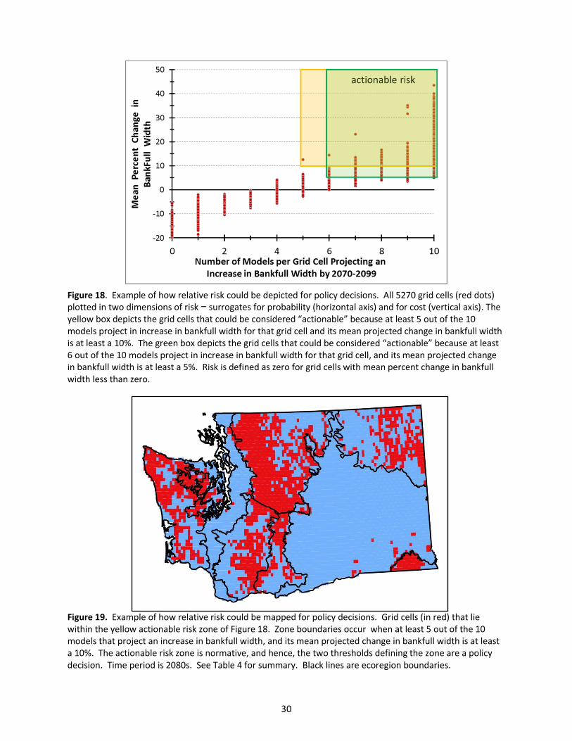
Our surrogates for probability and cost can be plotted in two dimensions for each grid cell (Figure 18). The relative locations of grid cells in the two-dimensional space represent the relative risk of culvert failure, i.e., the failure to pass fish during a particular time period. Within this space, managers can delineate their own zone of intolerable or actionable risk12, which is a policy decision based on normative values that will likely differ from one context to another. One manager, for instance, could believe that a culvert poses an actionable risk when the mean projected change in bankfull width is at least 10% and at least 5 models agree that bankfull width will increase. Another manager might want more certainty in the projections, and specify at least 6 models agreeing but also believe that 5% is a significant increase in bankfull width. These two actionable risk zones are shown in Figure 18. Grid cells in the actionable risk zone can then be mapped (Figures 19 and 20), and designs for new culverts built within those grid cells would incorporate projections of future percent change in bankfull width. Policy makers, managers, and engineers will ultimately need to decide how much projected change in bankfull width and how much certainty (i.e., model agreement) regarding increases in bankfull width equals an actionable risk.

12

We equate intolerable and actionable risk because the third characteristic of actionable risk is assumed to be true. That is, we assume that actions can be taken to eliminate or minimize the risk. Eliminating or minimizing risk of culvert failure entails installing a larger culvert.

27

Figure 15. The range of percent change in bankfull width for each grid cell for two time periods: A) 2040s and B) 2080s. Range equals the largest projection minus the smallest projection and is one way to express uncertainty. Black lines are ecoregion boundaries. Grid cells are 1/16-degree latitude x 1/16-degree longitude (approximately 5 x 7 km).

A

B

28

Figure 16. Number of models projecting an increase in bankfull width for each grid cell for two time periods: A) 2040s and B) 2080s. “Model agreement” is an expression of uncertainty. All models (10) or no models (0) projecting an increase indicates lowest uncertainty. Half of models (5) projecting an increase and half projecting a decrease in bankfull width indicates highest uncertainty. Black lines are ecoregion boundaries. Grid cells are 1/16-degree latitude x 1/16-degree longitude (approximately 5 x 7 km).

A

B

0 5 10

29

A

Figure 17. Distribution of projected percent change in bankfull width (BFW) between historical and 2040s time periods at (A) a grid cell in the Tucannon River Watershed and (B) a grid cell in the Finney Creek Watershed, a tributary to the Skagit River. Each black dot corresponds to a projection based on a different GCM. The red line indicates the mean of the 10 projections. Numbers in upper right corner of each graph are latitude and longitude of grid cell. The grid cell in the Tucannon River Watershed has 2 projections of approximately 38%. Mean estimates are the mean of 10 projections. Green box shows location of quartiles (i.e., interquartile range).

B

30

Figure 18. Example of how relative risk could be depicted for policy decisions. All 5270 grid cells (red dots) plotted in two dimensions of risk − surrogates for probability (horizontal axis) and for cost (vertical axis). The yellow box depicts the grid cells that could be considered “actionable” because at least 5 out of the 10 models project in increase in bankfull width for that grid cell and its mean projected change in bankfull width is at least a 10%. The green box depicts the grid cells that could be considered “actionable” because at least 6 out of the 10 models project in increase in bankfull width for that grid cell, and its mean projected change in bankfull width is at least a 5%. Risk is defined as zero for grid cells with mean percent change in bankfull width less than zero.

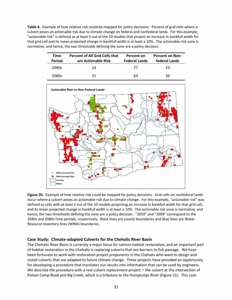
Figure 19. Example of how relative risk could be mapped for policy decisions. Grid cells (in red) that lie within the yellow actionable risk zone of Figure 18. Zone boundaries occur when at least 5 out of the 10 models that project an increase in bankfull width, and its mean projected change in bankfull width is at least a 10%. The actionable risk zone is normative, and hence, the two thresholds defining the zone are a policy decision. Time period is 2080s. See Table 4 for summary. Black lines are ecoregion boundaries.

31

Table 4. Example of how relative risk could be mapped for policy decisions. Percent of grid cells where a culvert poses an actionable risk due to climate change on federal and nonfederal lands. For this example, “actionable risk” is defined as at least 5 out of the 10 models that project an increase in bankfull width for that grid cell and its mean projected change in bankfull width is at least a 10%. The actionable risk zone is normative, and hence, the two thresholds defining the zone are a policy decision.

Time Period

Percent of All Grid Cells that are Actionable Risk

Percent on Federal Lands

Percent on Non-federal Lands

2040s 14 77 23

2080s 31 64 36

Figure 20. Example of how relative risk could be mapped for policy decisions. Grid cells on nonfederal lands occur where a culvert poses an actionable risk due to climate change. For this example, “actionable risk” was defined as cells with at least 5 out of the 10 models projecting an increase in bankfull width for that grid cell, and its mean projected change in bankfull width is at least a 10%. The actionable risk zone is normative, and hence, the two thresholds defining the zone are a policy decision. “2059” and “2099” correspond to the 2040s and 2080s time periods, respectively. Black lines are county boundaries and blue lines are Water Resource Inventory Area (WRIA) boundaries.

Case Study: Climate-adapted Culverts for the Chehalis River Basin The Chehalis River Basin is currently a major focus for salmon habitat restoration, and an important part of habitat restoration in the Chehalis is replacing culverts that are barriers to fish passage. We have been fortunate to work with restoration project proponents in the Chehalis who want to design and install culverts that are adapted to future climate change. These projects have provided an opportunity for developing a procedure that translates our results into information that can be used by engineers. We describe the procedure with a real culvert replacement project − the culvert at the intersection of Polson Camp Road and Big Creek, which is a tributary to the Humptulips River (Figure 21). This case

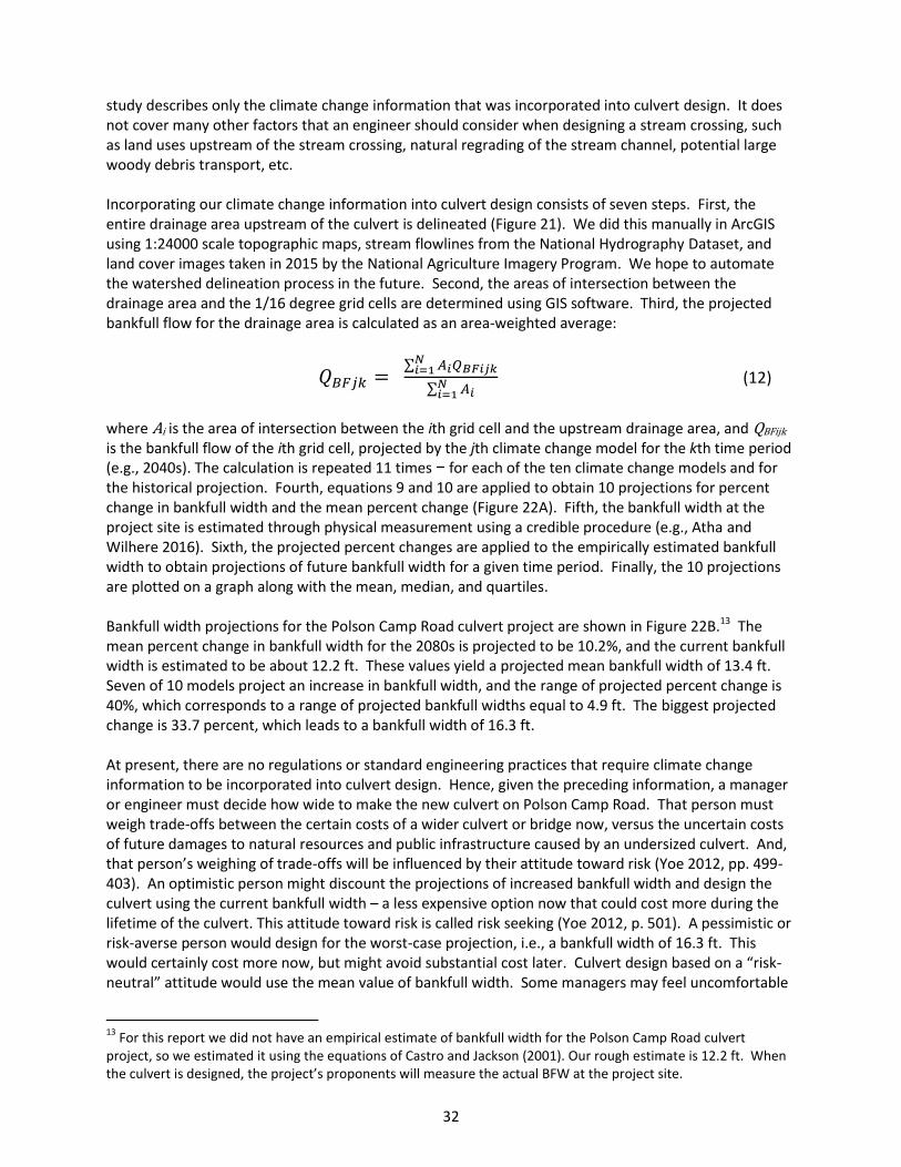
32

study describes only the climate change information that was incorporated into culvert design. It does not cover many other factors that an engineer should consider when designing a stream crossing, such as land uses upstream of the stream crossing, natural regrading of the stream channel, potential large woody debris transport, etc. Incorporating our climate change information into culvert design consists of seven steps. First, the entire drainage area upstream of the culvert is delineated (Figure 21). We did this manually in ArcGIS using 1:24000 scale topographic maps, stream flowlines from the National Hydrography Dataset, and land cover images taken in 2015 by the National Agriculture Imagery Program. We hope to automate the watershed delineation process in the future. Second, the areas of intersection between the drainage area and the 1/16 degree grid cells are determined using GIS software. Third, the projected bankfull flow for the drainage area is calculated as an area-weighted average:

𝑄𝐵𝐹𝑗𝑘 = ∑ 𝐴𝑖𝑄𝐵𝐹𝑖𝑗𝑘

𝑁𝑖=1

∑ 𝐴𝑖𝑁𝑖=1

(12)

where Ai is the area of intersection between the ith grid cell and the upstream drainage area, and QBFijk is the bankfull flow of the ith grid cell, projected by the jth climate change model for the kth time period (e.g., 2040s). The calculation is repeated 11 times − for each of the ten climate change models and for the historical projection. Fourth, equations 9 and 10 are applied to obtain 10 projections for percent change in bankfull width and the mean percent change (Figure 22A). Fifth, the bankfull width at the project site is estimated through physical measurement using a credible procedure (e.g., Atha and Wilhere 2016). Sixth, the projected percent changes are applied to the empirically estimated bankfull width to obtain projections of future bankfull width for a given time period. Finally, the 10 projections are plotted on a graph along with the mean, median, and quartiles. Bankfull width projections for the Polson Camp Road culvert project are shown in Figure 22B.13 The mean percent change in bankfull width for the 2080s is projected to be 10.2%, and the current bankfull width is estimated to be about 12.2 ft. These values yield a projected mean bankfull width of 13.4 ft. Seven of 10 models project an increase in bankfull width, and the range of projected percent change is 40%, which corresponds to a range of projected bankfull widths equal to 4.9 ft. The biggest projected change is 33.7 percent, which leads to a bankfull width of 16.3 ft. At present, there are no regulations or standard engineering practices that require climate change information to be incorporated into culvert design. Hence, given the preceding information, a manager or engineer must decide how wide to make the new culvert on Polson Camp Road. That person must weigh trade-offs between the certain costs of a wider culvert or bridge now, versus the uncertain costs of future damages to natural resources and public infrastructure caused by an undersized culvert. And, that person’s weighing of trade-offs will be influenced by their attitude toward risk (Yoe 2012, pp. 499-403). An optimistic person might discount the projections of increased bankfull width and design the culvert using the current bankfull width – a less expensive option now that could cost more during the lifetime of the culvert. This attitude toward risk is called risk seeking (Yoe 2012, p. 501). A pessimistic or risk-averse person would design for the worst-case projection, i.e., a bankfull width of 16.3 ft. This would certainly cost more now, but might avoid substantial cost later. Culvert design based on a “risk-neutral” attitude would use the mean value of bankfull width. Some managers may feel uncomfortable

13

For this report we did not have an empirical estimate of bankfull width for the Polson Camp Road culvert project, so we estimated it using the equations of Castro and Jackson (2001). Our rough estimate is 12.2 ft. When the culvert is designed, the project’s proponents will measure the actual BFW at the project site.

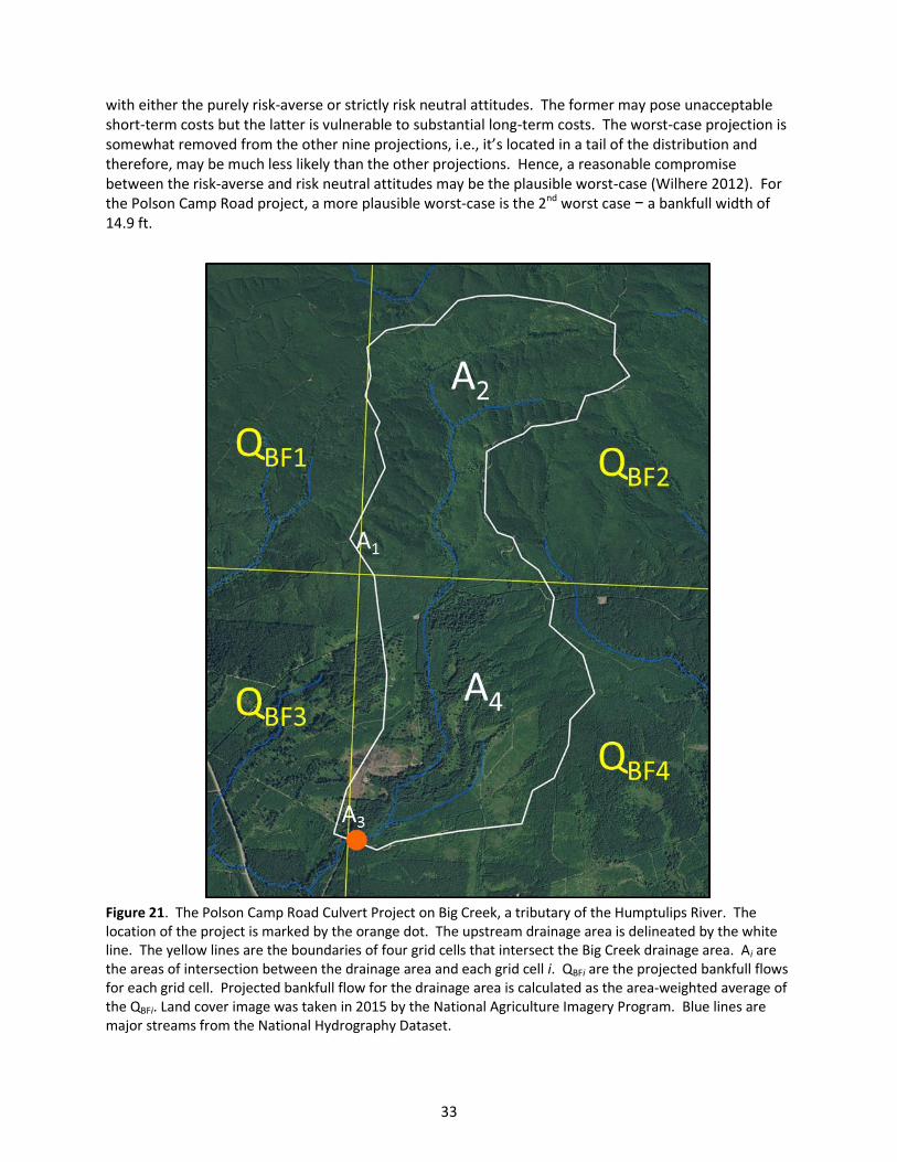
33

with either the purely risk-averse or strictly risk neutral attitudes. The former may pose unacceptable short-term costs but the latter is vulnerable to substantial long-term costs. The worst-case projection is somewhat removed from the other nine projections, i.e., it’s located in a tail of the distribution and therefore, may be much less likely than the other projections. Hence, a reasonable compromise between the risk-averse and risk neutral attitudes may be the plausible worst-case (Wilhere 2012). For the Polson Camp Road project, a more plausible worst-case is the 2nd worst case − a bankfull width of 14.9 ft.

Figure 21. The Polson Camp Road Culvert Project on Big Creek, a tributary of the Humptulips River. The location of the project is marked by the orange dot. The upstream drainage area is delineated by the white line. The yellow lines are the boundaries of four grid cells that intersect the Big Creek drainage area. Ai are the areas of intersection between the drainage area and each grid cell i. QBFi are the projected bankfull flows for each grid cell. Projected bankfull flow for the drainage area is calculated as the area-weighted average of the QBFi. Land cover image was taken in 2015 by the National Agriculture Imagery Program. Blue lines are major streams from the National Hydrography Dataset.

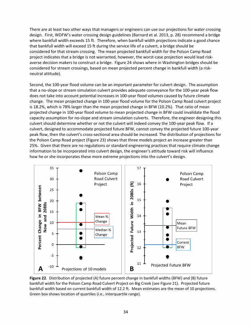
34

There are at least two other ways that managers or engineers can use our projections for water crossing design. First, WDFW’s water crossing design guidelines (Barnard et al. 2013, p. 28) recommend a bridge where bankfull width exceeds 15 ft. Therefore, when bankfull width projections indicate a good chance that bankfull width will exceed 15 ft during the service life of a culvert, a bridge should be considered for that stream crossing. The mean projected bankfull width for the Polson Camp Road project indicates that a bridge is not warranted, however, the worst-case projection would lead risk-averse decision makers to construct a bridge. Figure 24 shows where in Washington bridges should be considered for stream crossings, based on mean projected percent change in bankfull width (a risk-neutral attitude). Second, the 100-year flood volume can be an important parameter for culvert design. The assumption that a no-slope or stream simulation culvert provides adequate conveyance for the 100-year peak flow does not take into account potential increases in 100-year flood volumes caused by future climate change. The mean projected change in 100-year flood volume for the Polson Camp Road culvert project is 18.2%, which is 78% larger than the mean projected change in BFW (10.2%). That ratio of mean projected change in 100-year flood volume to mean projected change in BFW could invalidate the flood capacity assumption for no-slope and stream simulation culverts. Therefore, the engineer designing this culvert should determine whether or not the culvert will indeed convey the 100-year peak flow. If a culvert, designed to accommodate projected future BFW, cannot convey the projected future 100-year peak flow, then the culvert’s cross-sectional area should be increased. The distribution of projections for the Polson Camp Road project (Figure 23) shows that three models project an increase greater than 25%. Given that there are no regulations or standard engineering practices that require climate change information to be incorporated into culvert design, the engineer’s attitude toward risk will influence how he or she incorporates these more extreme projections into the culvert’s design. Figure 22. Distribution of projected (A) future percent change in bankfull widths (BFW) and (B) future bankfull width for the Polson Camp Road Culvert Project on Big Creek (see Figure 21). Projected future bankfull width based on current bankfull width of 12.2 ft. Mean estimates are the mean of 10 projections. Green box shows location of quartiles (i.e., interquartile range).

A B

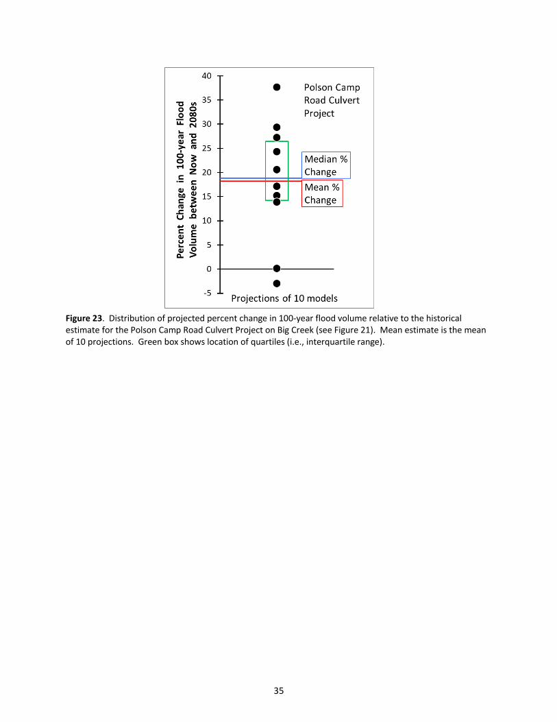
35

Figure 23. Distribution of projected percent change in 100-year flood volume relative to the historical estimate for the Polson Camp Road Culvert Project on Big Creek (see Figure 21). Mean estimate is the mean of 10 projections. Green box shows location of quartiles (i.e., interquartile range).

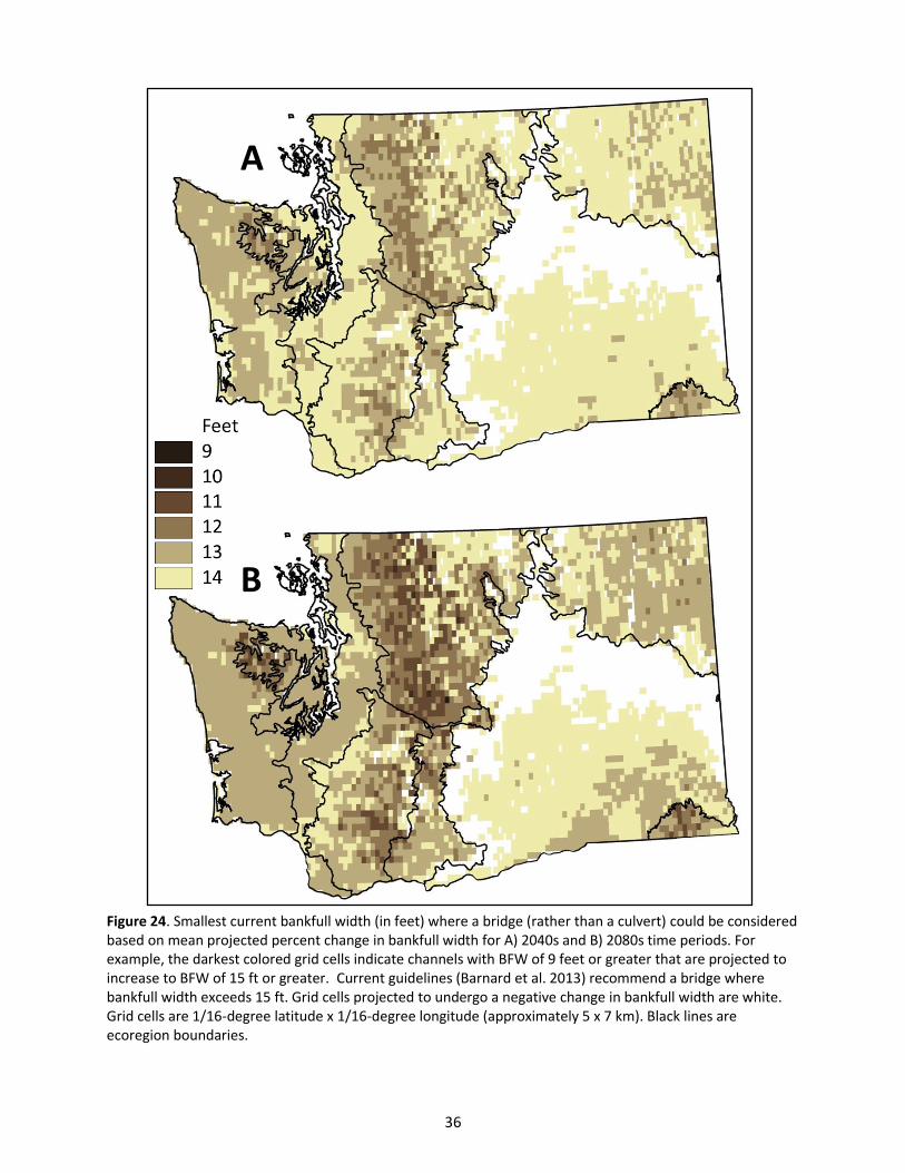
36

Figure 24. Smallest current bankfull width (in feet) where a bridge (rather than a culvert) could be considered based on mean projected percent change in bankfull width for A) 2040s and B) 2080s time periods. For example, the darkest colored grid cells indicate channels with BFW of 9 feet or greater that are projected to increase to BFW of 15 ft or greater. Current guidelines (Barnard et al. 2013) recommend a bridge where bankfull width exceeds 15 ft. Grid cells projected to undergo a negative change in bankfull width are white. Grid cells are 1/16-degree latitude x 1/16-degree longitude (approximately 5 x 7 km). Black lines are ecoregion boundaries.

A

B

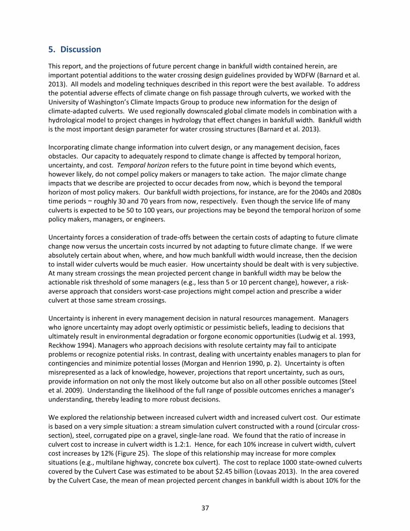
37

5. Discussion

This report, and the projections of future percent change in bankfull width contained herein, are important potential additions to the water crossing design guidelines provided by WDFW (Barnard et al. 2013). All models and modeling techniques described in this report were the best available. To address the potential adverse effects of climate change on fish passage through culverts, we worked with the University of Washington’s Climate Impacts Group to produce new information for the design of climate-adapted culverts. We used regionally downscaled global climate models in combination with a hydrological model to project changes in hydrology that effect changes in bankfull width. Bankfull width is the most important design parameter for water crossing structures (Barnard et al. 2013). Incorporating climate change information into culvert design, or any management decision, faces obstacles. Our capacity to adequately respond to climate change is affected by temporal horizon, uncertainty, and cost. Temporal horizon refers to the future point in time beyond which events, however likely, do not compel policy makers or managers to take action. The major climate change impacts that we describe are projected to occur decades from now, which is beyond the temporal horizon of most policy makers. Our bankfull width projections, for instance, are for the 2040s and 2080s time periods − roughly 30 and 70 years from now, respectively. Even though the service life of many culverts is expected to be 50 to 100 years, our projections may be beyond the temporal horizon of some policy makers, managers, or engineers. Uncertainty forces a consideration of trade-offs between the certain costs of adapting to future climate change now versus the uncertain costs incurred by not adapting to future climate change. If we were absolutely certain about when, where, and how much bankfull width would increase, then the decision to install wider culverts would be much easier. How uncertainty should be dealt with is very subjective. At many stream crossings the mean projected percent change in bankfull width may be below the actionable risk threshold of some managers (e.g., less than 5 or 10 percent change), however, a risk-averse approach that considers worst-case projections might compel action and prescribe a wider culvert at those same stream crossings. Uncertainty is inherent in every management decision in natural resources management. Managers who ignore uncertainty may adopt overly optimistic or pessimistic beliefs, leading to decisions that ultimately result in environmental degradation or forgone economic opportunities (Ludwig et al. 1993, Reckhow 1994). Managers who approach decisions with resolute certainty may fail to anticipate problems or recognize potential risks. In contrast, dealing with uncertainty enables managers to plan for contingencies and minimize potential losses (Morgan and Henrion 1990, p. 2). Uncertainty is often misrepresented as a lack of knowledge, however, projections that report uncertainty, such as ours, provide information on not only the most likely outcome but also on all other possible outcomes (Steel et al. 2009). Understanding the likelihood of the full range of possible outcomes enriches a manager’s understanding, thereby leading to more robust decisions. We explored the relationship between increased culvert width and increased culvert cost. Our estimate is based on a very simple situation: a stream simulation culvert constructed with a round (circular cross-section), steel, corrugated pipe on a gravel, single-lane road. We found that the ratio of increase in culvert cost to increase in culvert width is 1.2:1. Hence, for each 10% increase in culvert width, culvert cost increases by 12% (Figure 25). The slope of this relationship may increase for more complex situations (e.g., multilane highway, concrete box culvert). The cost to replace 1000 state-owned culverts covered by the Culvert Case was estimated to be about $2.45 billion (Lovaas 2013). In the area covered by the Culvert Case, the mean of mean projected percent changes in bankfull width is about 10% for the

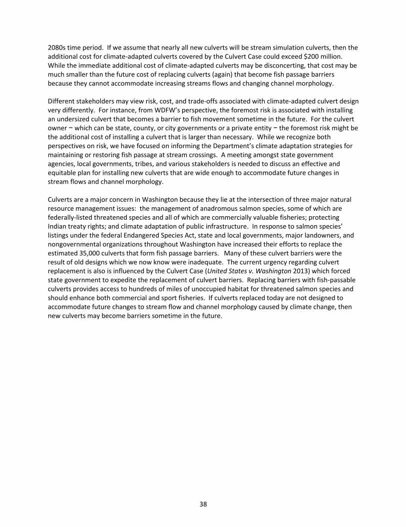
38

2080s time period. If we assume that nearly all new culverts will be stream simulation culverts, then the additional cost for climate-adapted culverts covered by the Culvert Case could exceed $200 million. While the immediate additional cost of climate-adapted culverts may be disconcerting, that cost may be much smaller than the future cost of replacing culverts (again) that become fish passage barriers because they cannot accommodate increasing streams flows and changing channel morphology. Different stakeholders may view risk, cost, and trade-offs associated with climate-adapted culvert design very differently. For instance, from WDFW’s perspective, the foremost risk is associated with installing an undersized culvert that becomes a barrier to fish movement sometime in the future. For the culvert owner − which can be state, county, or city governments or a private entity − the foremost risk might be the additional cost of installing a culvert that is larger than necessary. While we recognize both perspectives on risk, we have focused on informing the Department’s climate adaptation strategies for maintaining or restoring fish passage at stream crossings. A meeting amongst state government agencies, local governments, tribes, and various stakeholders is needed to discuss an effective and equitable plan for installing new culverts that are wide enough to accommodate future changes in stream flows and channel morphology. Culverts are a major concern in Washington because they lie at the intersection of three major natural resource management issues: the management of anadromous salmon species, some of which are federally-listed threatened species and all of which are commercially valuable fisheries; protecting Indian treaty rights; and climate adaptation of public infrastructure. In response to salmon species’ listings under the federal Endangered Species Act, state and local governments, major landowners, and nongovernmental organizations throughout Washington have increased their efforts to replace the estimated 35,000 culverts that form fish passage barriers. Many of these culvert barriers were the result of old designs which we now know were inadequate. The current urgency regarding culvert replacement is also is influenced by the Culvert Case (United States v. Washington 2013) which forced state government to expedite the replacement of culvert barriers. Replacing barriers with fish-passable culverts provides access to hundreds of miles of unoccupied habitat for threatened salmon species and should enhance both commercial and sport fisheries. If culverts replaced today are not designed to accommodate future changes to stream flow and channel morphology caused by climate change, then new culverts may become barriers sometime in the future.

39

Figure 25. Percent increase in culvert cost as a function of percent increase in culvert width. Relationship pertains to a stream simulation culvert for a gravel, single-lane road constructed with a round (circular cross-section), steel pipe.

6. Future Work

There are four categories of potential future work stemming from this project: 1) dissemination and use of this project’s products, 2) keeping abreast of relevant climate change science, 3) investigating the consequences of undersized culverts, and 4) developing more information to enrich the decision space. Nearly all future work related to this project is contingent upon new funding.

Dissemination of Project Results To more efficiently disseminate this project’s products we would like to develop an internet site. The simplest option is a website that allows users to download data files containing the projected percent changes in bankfull width for the entire state. A much more sophisticated option is a site that allows users to point-and-click on a culvert’s exact location. The site’s software then performs all of the calculations for determining projected percent change in bankfull width at that location (watershed delineation, area intersections, area-weighted average, etc.). Whatever internet-based service we develop, we will continue to work with proponents of culvert projects to help them design climate-adapted culverts. To encourage greater use of this project’s products, we hope to add a chapter on climate adaptation to WDFW’S current water crossing design guidelines (Barnard et al. 2013). That chapter would explain the information that we have developed and explain how to incorporate it into culvert or bridge design. It would also cover how to use the results of the 100-year flood analysis in water crossing design.

Updating Climate Science Climate change science is one of the hottest topics in science, and consequently, it is constantly advancing. New climate change projections are produced periodically, and we hope that CIG updates

40

their state-wide hydrological projections as new climate change projections become available. Updates are especially important because CIG’s current state-wide projections were generated with models that did not include extreme precipitation events. A major issue in climate change modelling is the best way to express uncertainty. We followed recommendations for expressing uncertainty (Kandlikar et al. 2005, Tebaldi et al. 2011), but current methods are not entirely satisfactory. As methods for expressing uncertainty advance, we hope to incorporate those advances. We could also explore enhancements to the hydrological modelling. Land cover is a major variable in VIC, but we currently use 1992-1993 land cover data which are also static in time. We could simulate changes in land use like increased urbanization, and the resulting hydrological response over time.

Understanding the Consequences of Undersized Culverts With respect to culverts and climate change, WDFW’s principal concern is the loss of fish passage and damage to fish habitat caused by undersized culverts. At present, we use the ratio of future to current bankfull width as a surrogate for future potential cost, i.e., harm to fish populations as a result of not installing a wider culvert or bridge. We must use a surrogate for damage or harm because we lack empirically-derived relationships that describe how fish passage changes as a function of the culvert-channel width disparity. In fact, there are no empirical studies describing stream channel behavior in no-slope culverts and only one inconclusive study on stream channel behavior in stream simulation culverts (Barnard et al. 2015). Hence, we do not fully understand how increases in the channel-culvert width disparity affect movement, scour, or aggradation of sediment and consequent fish passability. Lacking this knowledge, we cannot estimate the actual risk of undersized culverts due to climate change. There are two approaches for closing this knowledge gap. The first is modelling stream flow and sediment transport in culverts (e.g., Rowley et al. 2014). We have explored the acquisition and use of two-dimensional simulation models of sediment transport but currently lack funding to pursue such work. The second approach is empirical study. We are currently in the fourth year of long-term effective monitoring of recently installed no-slope and stream simulation culverts. Some questions about the relationships between culvert width and sediment transport can be answered through long-term monitoring.

Improving Information on risk and cost The information we have developed for designing climate adapted culverts should be considered the best-available science on this issue. However, we do not provide key information that many decision makers would like to have when considering the risk, cost, and trade-offs associated with climate-adapted culvert design. As explained above, we have only a simplistic estimate for the cost of installing wider culverts and we cannot currently project the all ecological consequences of an undersized culvert. To address the former, we could develop cost estimates for a wide variety of culvert replacement situations. To address the latter, computer modelling may be the best short-term approach. We would like to tackle both tasks, but that is contingent upon funding.

7. Acknowledgements The primary authors of this report were George Wilhere, Jane Atha and Timothy Quinn, all of WDFW. Other project team members and contributors were Lynn Helbrecht, Kevin Lautz and Don Ponder from WDFW, Jennie Hoffman (Adaptation Insight) and Ingrid Tohver (Climate Impacts Group). We also thank Sean Stanley, civil engineer at WDFW, who provided cost estimates for wider culverts and Bob Vadas Jr. at WDFW for reviewing the final draft manuscript. We thank Guillaume Mauger (Climate Impacts Group) who provided information and answered many of our questions about climate and hydrological projections. David Price, Restoration Section manager at WDFW, made essential contributions toward promoting climate-adapted culverts in the Chehalis River Basin. We thank him for giving us an opportunity to apply our results to actual culvert design. We also thank Janine Castro at U.S. Fish &

41

Wildlife Service for answering questions and offering advice on the use of her research results. Finally, we thank the North Pacific Landscape Conservation Cooperative for providing foundational funding for this project through a grant awarded to Timothy Quinn and Lynn Helbrecht.

8. References Allmendinger, N.W., J.E. Pizzuto, N. Potter, T.W. Johnson, W.C. Hession. 2005. The influence of riparian vegetation on stream width, eastern Pennsylvania, USA. Geological Society of America Bulletin 117:229-243. Atha, J.B., and G.F. Wilhere. 2015. Bankfull width estimation procedure for culvert design and monitoring. Habitat Program, Washington Department of Fish and Wildlife, Olympia, WA. Barnard, R.J., J. Johnson, P. Brooks, K.M. Bates, B. Heiner, J.P. Klavas, D.C. Ponder, P.D. Smith, and P.D. Powers. 2013. Water Crossings Design Guidelines. Washington Department of Fish and Wildlife, Olympia, WA. Barnard, R.J., S. Yokers, A. Nagygyor, and T. Quinn. 2015. An evaluation of the stream simulation culvert design method in Washington State. River Research and Applications. 31:1376-1387. Battin, J., M.W. Wiley, M.H. Ruckelshaus, R.N. Palmer, E. Korb, K.K. Bartz, and H. Imaki. 2007. Projected impacts of climate change on salmon habitat restoration. Proceedings of the National Academy of Sciences of United States of America 104:6720–6725. Beechie, T.J., M. Ruckelshaus, E. Buhle, A. Fullerton, and L. Holsinger. 2006. Hydrologic regime and the conservation of salmon life history diversity. Biological Conservation 130:560–572. Buffington, J.M. 2012. Changes in channel morphology over human time scales. pp. 435-463 in M. Church, P.M. Biron, and A.G. Roy (eds.). Gravel-bed rivers: processes, tools, environments. John Wiley & Sons, Hoboken, NJ. Castro, J. M. and P. L. Jackson. 2001. Bankfull discharge recurrence intervals and regional hydraulic geometry relationships: patterns in the Pacific Northwest, USA. Journal of the American Water Resources Association 37:1249–1262. Cenderelli, D., K. Clarkin, R. Gubernick and M. Weinhold. 2011. Stream simulation for aquatic organism passage at road-stream crossings. Transportation Research Record: Journal of the Transportation Research Board 2203:36-45. Chelgren, N.D. , and J.B. Dunham. 2015. Connectivity and conditional models of access and abundance of species in stream networks. Ecological Applications 25:1357–1372. CHG. 2016. VIC Model Overview. Computational Hydrology Group, Dept. of Civil and Enviromental Engineering, University of Washington, Seattle, WA. accessed at http://vic.readthedocs.io/en/master/Overview/ModelOverview/. Church, M. 1995. Geomorphic response to river flow regulation: case studies and time-scales. Regulated Rivers: Research and Management 11:3-22.

42

Coulthard, T., J. Ramirez, H. Fowler and V. Glenis. 2012. Using the UKCP09 probabilistic scenarios to model the amplified impact of climate change on drainage basin sediment yield. Hydrology and Earth System Sciences 16:4401-4416. DNR. 1999. Forests and Fish Report. Forest Practices Division, Washington State Department of Natural Resources, Olympia, WA. Dunham, J. B., G. L. Vinyard, and B. E. Rieman. 1997. Habitat fragmentation and extinction risk of Lahontan cutthroat trout. North American Journal of Fisheries Management 17:1126–1133. Dunne, T. and L. B. Leopold. 1978. Water in environmental planning. Macmillan, New Rork, NY. Eaton, B.C. 2013. Hydraulic geometry: empirical investigations and theoretical approaches. p. 313-329 in E. Wohl (ed.). Treatise on Fluvial Geomorphology. Elsevier, Amsterdam. Ellis, W.H., and D. M. Gray. 1966. Interrelationships between the peak instantaneous and average daily discharges of small prairie streams. Candian Agricultural Engineering February:1-4. Elsner, M.M., L. Cuo, N. Voisin, J.S. Deems , A.F. Hamlet , J.A. Vano , K.E.B. Mickelson , S.Y. Lee, D.P. Lettenmaier. 2010. Implications of 21st century climate change for the hydrology of Washington State. Climatic Change 102:225–260. Ficke A.D., C.A. Myrick, and L.J. Hansen . 2008. Potential impacts of global climate change on freshwater fisheries. Reviews in Fish Biology and Fisheries 17:581–613. Fill, H.D., and A.A. Steiner. 2003. Estimating instantaneous peak flow from mean daily flow data. Journal of Hydrological Engineering 8:365-370. Fuller, W.E., 1914. Flood flows. Transactions of the American Society of Civil Engineers 77:564-617. GAO. 2001. Land management agencies: restoring fish passage through culverts on Forest Service and BLM lands in Oregon and Washington Could Take Decades. GAO-02-136. General Accounting Office, Washington, DC. Gillespie, N., A. Unthank, L. Campbell, P. Anderson, R. Gubernick, M. Weinhold, D. Cenderelli, B. Austin, D. McKinley and S. Wells. 2014. Flood Eefects on road-stream crossing infrastructure: economic and ecological benefits of stream simulation designs. Fisheries 39(2):62-76. Gleason, C.J. 2015. Hydraulic geometry of natural rivers: a review and future directions. Progress in Physical Geography 39:337-360. Gomez, B., Y. Cui, A. Kettner, D. Peacock and J. Syvitski. 2009. Simulating changes to the sediment transport regime of the Waipaoa River, New Zealand, driven by climate change in the twenty-first century. Global and Planetary Change 67:153-166. Governor’s Salmon Recovery Office. 2008. State of the salmon in watersheds report. Governor’s Salmon Recovery Office, Olympia, WA.

43

Granshaw, F.D., and A.G. Fountain. 2006. Glacier change (1958–1998) in the North Cascades National Park Complex, Washington, USA. Journal of Glaciology 52:251−256. Gray, D.M. 1973. Handbook of the principles of hydrology. Water Information Center, Huntington, NY. Hamlet, A.F., P. Carrasco, J. Deems, M.M. Elsner, T. Kamstra, C. Lee, S.-Y. Lee, G. Mauger, E.P. Salathe, I. Tohver, and L.W. Binder, 2010. Final project report for the Columbia Basin climate change scenarios project. Climate Impacts Group, University of Washington, Seattle. Hamlet, A.F., M.M. Elsner, G. Mauger, S.-Y. Lee, and I.M. Tohver, 2013. An overview of the Columbia Basin climate change scenarios project: approach, methods, and summary of key results. Atmosphere-Ocean 51:392-415. Hamlet, A. F., P.W. Mote, M.P. Clark and D.P. Lettenmaier. 2007. Twentieth-century trends in runoff, evapotranspiration, and soil moisture in the western United States. Journal of Climate 20:1468-1486. Hansen, M.C., R.S. DeFries, J.R. G. Townshend, and R. Sohlberg. 2000. Global land cover classification at 1 km spatial resolution using a classification tree approach. International Journal of Remote Sensing, 21:1331-1364. Hosking, J.R.M. 2015. L-moments. R package, version 2.5. URL: http://CRAN.R-project.org/package=lmom. IGES. 2012. Executive roundtable on climate, private sector engagement, and strategic forecasting. Institute for Global Environmental Strategies, Arlington, VA. IPCC. 2007. Summary for policymakers. A report of Working Group I of the Intergovernmental Panel on Climate Change. pp. 1-18 in Climate Change 2007: The Physical Science Basis. Cambridge Univ. Press, Cambridge, U.K. IPCC. 2010. Good pratice guidance paper on assessing and combining multi model climate projections. Meeting report of IPCC expert meeting in assessing and combining multi model climate projections. IPCC Working Group I Techicnal Support Unit, University of Bern, Bern, Switzerland. Kalaney E et al. 1996. The NCEP/NCAR 40-year reanalysis project. Bulletin of the American Meteorological Society 77:437–471. Kandlikar M., J. Risbey, and S. Dessai. 2005. Representing and communicating deep uncertainty in climate change assessment. Comptes Rendus Geoscience 337:443–455. Kilgore, R.T., D.B. Thompson, D.T. Ford. 2013. Estimating joint probabilities of design coincident flows at stream confluences. National Cooperative Highway Research Program, Transportation Research Board, National Research Council, Washington, DC. Knighton, D. 1998. Fluvial Forms and Processes: A New Perspective. Arnold, London. Knutti, R. 2010. The end of model democracy? Climate Change 102:395-404.

44

Knutti R., R. Furrer, C. Tebaldi, J. Cermak and G.A. Meehl. 2010. Challenges in combining projections from multiple climate models. Journal of Climate 23:2739–2758. Kruse, C. G., W.A. Hubert, and F.J. Rahel. 2001. An assessment of headwater isolation as a conservation strategy for cutthroat trout in the Absaroka Mountains of Wyoming. Northwest Science 75:1–11. Lambereti, G.A., S.V. Gregory, L.R. Ashkenas, R.C. Wildman, K.M.S. Moore. 1991. Stream ecosystem recovery following a catastrophic debris flow. Canadian Journal of Fisheries and Aquatic Sciences 48: 196–208. Lane, S., V. Tayefi, S. Reid, D. Yu and R. Hardy. 2007. Interactions between sediment delivery, channel change, climate change and flood risk in a temperate upland environment. Earth Surface Processes and Landforms 32:429-446. Lee, S-Y, A.F. Hamlet, and E.E. Grossman. 2016. Impacts of climate change on regulated streamflow, hydrologic extremes, hydropower production, and sediment discharge in the Skagit River Basin. Northwest Science 90:23-43. Leopold, L. B. and T. Maddock. 1953. The hydraulic geometry of stream channels and some physiographic implications. U.S. Geological Survey Professional Paper 252. United States Government Printing Office, Washington, DC. Liang, X., D.P. Lettenmaier, E.F. Wood, S.J. Burges. 1994. A simple hydrologically based model of land wurface water and energy fluxes for general circulation models. Journal of Geophysical Research 99 (D7):14,415-14,428. Littell, J.S., M. McGuire Elsner, L.C. Whitely Binder, and A.K. Snover (eds). 2009. The Washington climate change impacts assessment: evaluating Washington's future in a changing climate. Climate Impacts Group, University of Washington, Seattle, WA. Lovass, J. 2013. ‘Culvert case’ could be costly issue for state. Olympian, April 13, 2013. Ludwig, D., R. Hilborn, and C. Walters. 1993. Uncertainty, resource exploitation, and conservation: lessons from history. Science 260:17-36. Magilligan, F. J., J. D. Phillips, L. A. James and B. Gomez. 1998. Geomorphic and sedimentological controls on the effectiveness of an extreme flood. The Journal of Geology 106:87-96. Mantua, N., I. Tohver and A. Hamlet. 2010. Climate change impacts on streamflow extremes and summertime stream temperature and their possible consequences for freshwater salmon habitat in Washington State. Climatic Change 102:187-223. Mauger, G.S., J.H, Casola, H.A. Morgan, R.L. Strauch, B. Jones, B. Curry, T.M. Busch Isaksen, L. Whitely Binder, M.B. Krosby, and A.K. Snover. 2015. State of knowledge: climate change in Puget Sound. Climate Impacts Group, University of Washington, Seattle, WA. Maurer, E. P., A.W. Wood, J.C. Adam, D.P. Lettenmaier, and B. Nijssen. 2002. A long-term hydrologically-based data set of land surface fluxes and states for the conterminous United States. Journal of Climate 15:3237–3251.

45

Meehl, G.A., C. Covey, T. Delworth, M. Latif, B. McAvaney, J.F.B. Mitchell, R.J. Stouffer, and K.E. Taylor 2007. The WCRP CMIP3 multi-model dataset: a new era in climate change research. Bulletin of the American Meteorological Society 88:1383-1394. Modarres, M., M. Kaminskiy, and V. Krivtsov. 1999. Reliability engineering and risk analysis: a practical guide. Marcel Dekker Inc., New York, NY. Morgan, M. G., and M. Henrion. 1990. Uncertainty: a guide to dealing with uncertainty in quantitative risk and policy analysis. Cambridge University Press, Cambridge, United Kingdom. Mote, P.W., and E.P. Salathé. 2010. Future climate in the Pacific Northwest. Climate Change 102:29-50. NAACC. 2016. Implementing Codes and Standards. North Atlantic Landscape Conservation Cooperative, University of Massachussets, Amherst, MA. accessed at https://streamcontinuity.org/resources/crossings_toolkit/impl_codes_standards.htm. Nakicenovic, N., J. Alcamo, G. Davis, B. de Vries, J. Fenhann, S. Gaffin, K. Gregory, A. Grübler et al. 2000. Emission scenarios. A Special Report of Working Group III of the Intergovernmental Panel on Climate Change. Cambridge University Press, Cambridge, UK. NCHRP. 2015. Service life of culverts: a synthesis of highway practice. National Cooperative Highway Research Program, Transportation Research Board, National Research Council, Washington, DC. Neiman P. J., L.J. Schick, F.M. Ralph, M. Hughes, and G.A. Wick. 2011. Flooding in western Washington: the connection to atmospheric rivers. Journal of Hydrometeorology 12:1337–58. Neville, H., J. B. Dunham, A. Rosenberger, J. Umek, and B. Nelson. 2009. Influences of wildfire, habitat size, and connectivity on trout in headwater streams revealed by patterns of genetic diversity. Transactions of the American Fisheries Society 138:1314–1327. Nijssen, B., D.P. Lettenmaier, X. Liang, S.W. Wetzel, and E.F. Wood. 1997, Streamflow simulations for continental-scale river basins. Journal of the American Water Resources Association 36:399-420. Parker, W.S. 2010. Predicting weather and climate: uncertainty, ensembles and probability. Studies in History and Philosophy of Modern Physics 41:263-272. Parker, W.S. 2013. Ensemble modeling, uncertainty, and robust predictions. WIREs Climate Change 4:213-223. Praskievicz, S. 2015. A coupled hierarchical modeling approach to simulating the geomorphic response of river systems to anthropogenic climate change. Earth Surface Processes and Landforms 40:1616-1630. Price, D.M., T. Quinn, and R.J. Barnard. 2010. Fish passage effectiveness of recently constructed road crossing culverts in the Puget Sound Region of Washington State. North American Journal of Fisheries Management 30:1110-1125.

46

Randall D.A., R.A. Wood, S. Bony, R. Colman, T. Fichefet, J. Fyfe, V. Kattsov, A. Pitman, J. Shukla, J. Srinivasan, R.J. Stouffer, A. Sumi, and K.E. Taylor. 2007. Climate models and their evaluation. pp. 591-662 in S. Solomon, D. Qin, M. Manning, Z. Chen, M. Marquis, K.B. Averyt, M.Tignor and H.L. Miller (eds). Climate change 2007: the physical science basis. Contribution of working group I to the fourth assessment report of the Intergovernmental Panel on Climate Change. Cambridge University Press, Cambridge, UK. Reagan, R.E. 2015 Where the stream meets the road: prioritizing culvert replacement for fish passage. Master’s Thesis. Oregon State University, Corvallis, OR. Reckhow, K. H. 1994. Importance of scientific uncertainty in decision making. Environmental Management 18:161–166. Reeves, G. H., L.E. Benda, K.M. Burnett, P.A. Bisson, and J.R. Sedell. 1995. A disturbance-based ecosystem approach to maintaining and restoring freshwater habitats of evolutionarily significant units of anadromous salmonids in the Pacific Northwest. pp. 334–349 in J.L. Nielsen (ed). Evolution and the aquatic ecosystem: defining unique units in population conservation. Symposium 17. American Fisheries Society, Bethesda, MD. Rieman, B.E., and J.B. Dunham. 2000. Metapopulations and salmonids: a synthesis of life history patterns and empirical observations. Ecology of Freshwater Fish 9:51-64. Rowley, K.J., and R.H. Hotchkiss. 2014. Sediment transport conditions near culverts. pp. 1402-1411 in Proceedings of World Environmental and Water Resources Congress, American Society of Civil Engineers. Salathé Jr., E.P., A.F. Hamlet, C.F. Mass, S.-Y. Lee, M. Stumbaugh, and R. Steed. 2014. Estimates of twenty-first-century flood risk in the Pacific Northwest based on regional climate model simulations. Journal of Hydrometeorology 15: 1881-1899. Salathè, E.P., P.W. Mote, and M.W. Wiley. 2007. Review of scenario selection and downscaling methods for the assessment of climate change impacts on hydrology in the United States Pacific Northwest. International Journal of Climatology 27:1611-1621. Schindler, D. E., X. Augerot, E. Fleishman, N. J. Mantua, B. Riddell, M. Ruckelshaus, J. Seeb, and M. Webster. 2008. Climate change, ecosystem impacts, and management for Pacific salmon. Fisheries 33(10):502–506. Sheer, M.B., and E.A. Steel. 2006. Lost watersheds: barriers, aquatic habitat connectivity, and salmon persistence in the Willamette and Lower Columbia River basins. Transactions of the American Fisheries Society 135:1654-1669. Simon, A., W. Dickerson and A. Heins (2004). Suspended-sediment transport rates at the 1.5-year recurrence interval for ecoregions of the United States: transport conditions at the bankfull and effective discharge? Geomorphology 58:243-262. Singh, V.P. 2003. On the theories of hydraulic geometry. International Journal of Sediment Research 18:196-218.

47

Sitts D., A.G. Fountain, and M. Hoffman. 2010. Twentieth century glacier change on Mount Adams, Washington, USA. Northwest Science 84:378–385. Steel, E.A., T.J. Beechie, M.H. Ruckelshaus, A.H. Fullerton, P. McElhany, and P. Roni. 2009. Mind the gap: uncertainty and model communication between mangers and scientists. American Fisheries Society Symposium 71:357–372. Stephens, E.M., T.L. Edwards, and D. Demeritt. 2012. Communicating probabilistic information from climate model ensembles − lessons from numerical weather prediction. WIREs Climate Change 3:409-426. Stephenson D.B., M. Collins, J.C. Rougier, and R.E. Chandler. 2012. Statistical problems in the probabilistic prediction of climate change. Environmetrics 23:364–372. Stewart, I.T., D.R. Cayan, and M.D. Dettinger. 2005. Changes toward earlier streamflow timing across western North America. Journal of Climate 18:1136-1155. Stoelinga, M.T.,M.D. Albright, and C. F.Mass. 2010. A new look at snowpack trends in the Cascade Mountains. Journal of Climate 23:2473-2491. Taugas, E.V., J.L. Ayuso, A. Pena, Y. Yuan, M.C. Sanchez, J.V. Giraldez, ansd R. Perez. 2008. Testing the relationship between instantaneous peak flow and mean daily flow in a Mediterranean area southeast Spain. Catena 75:129-137.

Tebaldi, C., J.M. Arblaster, and R. Knutti. 2011. Mapping model agreement on future climate projections, Geophysical Research Letters 38, L23701, doi:10.1029/2011GL049863.

Tebaldi, C., and R. Knutti. 2007. The use of the multi-model ensembel in probabilistic climate projections. Philosophical Transactions of the Royal Society (A) 365:2053-2075.

Tohver, I., A.F. Hamlet, and S-Y. Lee. 2014. Impacts of 21st century climate change on hydrologic extremes in the Pacific Northwest region of North America. Journal of the American Water Resources Association 50:1461-1476.

Tohver, I., S-Y. Lee, and A.F. Hamlet. 2012. Using physically based hydrology models to improve fine scale estimates of Q100 in complex mountain terrain. Final project report. Climate Impacts Group, Department of Civil and Environmental Engineering, University of Wahington, Seattle.

United States v. Washington. 1980. 506 F. Supp. 187 (W.D. Wash.).

United States v. Washington. 2013. Case No. CV 70-9213 (W.D. Wash.).

USACE. 2016. Special public notice: nationwide permit reissuance request for comments. U.S. Army Corps of Engineers, Seattle District, WA. Van Vuuren, D. P., Edmonds, J., Kainuma, et al. 2011. The representative concentration pathways: an overview. Climatic Change 109:5-31. Warner, M.D., C.F. Mass, and E.P. Salathé. 2015. Changes in winter atmospheric rivers along the North American west coast in CMIP5 climate models. Journal of Hydrometeorology. 16:118-128.

48

WDFW. 2006. Status of the hydraulic project approval administration: report to the Office of Financial Management. Washington Department of Fish and Wildlife, Olympia, WA. WDFW. 2009. Fish Passage and Surface Water Diversion Screening Assessment and Prioritization Manual. Washington Department of Fish and Wildlife, Olympia, WA. WSDOT. 2015. Hydraulics manual. Environmental and Engineering Program, Washington State Department of Transportation, Olympia, WA. Wilhere, G.F. 2012. Using Bayesian networks to incorporate uncertainty in habitat suitability index models. Journal of Wildlife Management 76:1298-1309. Winston, M.R., C. M. Taylor, and J. Pigg. 1991. Upstream extirpation of four minnow species due to damming of a prairie stream. Transactions of the American Fisheries Society 120:98–105. Wofford, J. E. B., R. E. Gresswell, and M. A. Banks. 2005. Influence of barriers to movement on within-watershed genetic variation of coastal cutthroat trout. Ecological Applications 15:628–637.

Wohl, E., 2014. Rivers in the landscape: science and management. John Wiley & Sons.

Wolman, M. G. and J. P. Miller (1960). Magnitude and frequency of forces in geomorphic processes. The Journal of Geology 68:54-74.

Yoe, C. 2012. Principles of risk analysis: decision making under uncertainty. CRC Press, Boca Raton, FL.