Incorporating Bioassessment Using Freshwater Algae into California’s Surface Water Ambient Monitoring Program (SWAMP)

May 2008

2008 Technical Report

This project was funded by SWAMP.

ACKNOWLEDGEMENTS

The authors wish to thank the members of our Technical Advisory Committee for assisting with the development of the content for this document and reviewing/commenting on draft versions. The committee members are listed below, in alphabetical order: E. Paulette Akers Kentucky Division of Water Quality Amanda Bern State Water Resources Control Board Lilian Busse San Diego Regional Water Quality Control Board Steve Camacho State Water Resources Control Board Matthew Cover University of California, Berkeley Clayton Creager North Coast Regional Water Quality Control Board David Herbst Sierra Nevada Aquatic Research Laboratory Emily Hollingsworth South Carolina Dept. of Health & Environmental Control Marc Los Huertos California State University, Monterey Bay Michael Lyons Los Angeles Regional Water Quality Control Board Peter Ode California Department of Fish and Game Emilie Reyes State Water Resources Control Board Fraser Shilling University of California, Davis Marco Sigala Moss Landing Marine Laboratories Eric Stein Southern California Coastal Water Research Project Thomas Suk Lahontan Regional Water Quality Control Board Martha Sutula Southern California Coastal Water Research Project Karen Taberski San Francisco Bay Regional Water Quality Control Board Karen Vargas Bureau Water Quality Planning, Nevada Div. Env. Protection Pavlova Vitale Santa Ana Regional Water Quality Control Board Christine Weilhoefer United States Environmental Protection Agency

i

LIST OF ACRONYMS

ABL Aquatic Bioassessment Laboratory AFDM Ash-free Dry Mass ALU Aquatic Life Uses BMI Benthic Macroinvertebrate CMAP California Monitoring and Assessment Program CRAM California Rapid Assessment Method CS Coastal Southern part of the State (currently developing algae indices) CWAM California Watershed Assessment Manual DO Dissolved Oxygen EMAP Environmental Monitoring and Assessment Program EU European Union HABs Harmful Algal Blooms IBI Index of Biotic Integrity LR Lahontan Region (where a preliminary algal index has been developed) MLOEs Multiple Lines of Evidence NAEMP National Aquatic Ecosystem Monitoring Program (South Africa) NAWQA National Water Quality Assessment Program NNE Nutrient Numeric Endpoint NPDES National Pollutant Discharge Elimination System O/E Observed/Expected PHab Physical Habitat PSA Perennial Stream Assessment QAPP Quality Assurance Project Plan RCMP Reference Condition Management Program RIVPACS River Invertebrate Prediction and Classification System RWQCB Regional Water Quality Control Board SAFIT Southwest Association of Freshwater Invertebrate Taxonomists SCCWRP Southern California Coastal Water Research Project SEM Scanning Electron Microscope/Microscopy SMC Stormwater Monitoring Coalition SNARL Sierra Nevada Aquatic Research Laboratory SWAMP Surface Water Ambient Monitoring Program SWRCB State Water Resources Control Board TAC Technical Advisory Committee TMDL Total Maximum Daily Load USEPA United States Environmental Protection Agency USGS United States Geological Survey WFD Water Framework Directive (European Union)

ii

TABLE OF CONTENTS

Acknowledgements........................................................................................................................ i List of Acronyms ........................................................................................................................... ii Table of Contents......................................................................................................................... iii Executive Summary ......................................................................................................................1 Introduction and Problem Statement ............................................................................................4 Objectives and Guiding Principles ................................................................................................6 Algal Assemblages as Bioindicators .............................................................................................8

Definition of Algae.....................................................................................................................8 Benefits of Algae-based Bioassessment...................................................................................9

Applications of Algae for Bioassessment....................................................................................12 Use of Algae by Other States and Countries ..........................................................................12 Development and Implementation of Algae-based Bioassessment in California....................13 Integration and Leveraging with Existing Bioassessment .......................................................15

Technical Issues and Recommendations for Indicator Development and Implementation.........17 Potential Indicators: Pros and Cons........................................................................................17 Types and Applications of Algal Indicators .............................................................................20

Measurement of biomass....................................................................................................20 Choice of algal assemblage ................................................................................................21 Laboratory and taxonomic issues .......................................................................................23

Sampling Issues......................................................................................................................24 Sampling design..................................................................................................................24 Additional parameters to measure in the field.....................................................................26

Analytical Issues .....................................................................................................................27 Assemblage data reduction and interpretation....................................................................27 Examples of metrics used in algal IBIs ...............................................................................27 Reference sites ...................................................................................................................29

Integration with Other Biomonitoring Data ..................................................................................31 Complementarity of Bioindicators – Responses to Stress ......................................................31 Complementarity of Bioindicators – Varying Temporal Scales ...............................................31

Summary of Recommendations..................................................................................................33 Appendix A: Summary of Algal Bioassessment in Other States............................................. A - 1 Appendix B: Summary of Algal Bioassessment in Selected Other Countries......................... B - 1 Appendix C: Example of a Protocol for Sampling Algae......................................................... C - 1

iii

EXECUTIVE SUMMARY

This document was written to assist California’s State Water Resources Control Board (SWRCB) with incorporating algae into the bioassessment toolbox of the Surface Water Ambient Monitoring Program (SWAMP). It represents a consensus among members of a Technical Advisory Committee (TAC) regarding the best next steps toward implementation of algal bioassessment in the State. Recommendations were based on a combination of 1) information gathered from an extensive literature review, 2) a survey of algal bioassessment efforts that have occurred in parts of California and of programs in other states and countries, and 3) the best professional judgment of TAC members. We recommend that the State include algae as a component of SWAMP monitoring, in terms of both algal biomass and taxonomic composition of algal assemblages, the latter of which can be used in Indices of Biotic Integrity (IBIs). Algae will provide information beyond that which is currently obtainable through bioassessment with benthic macroinvertebrates (BMIs) alone. The following are some of the advantages to including algae in SWAMP monitoring:

• Addition of an algal component to SWAMP bioassessment (in which BMIs are currently the sole bioindicator) will satisfy the United States Environmental Protection Agency (USEPA) recommendation to utilize multiple bioindicators, and will facilitate the “weight-of-evidence” approach to interpretation of biomonitoring results. This approach involves interpreting data from multiple sources to arrive at conclusions about an environmental system or stressor. Multiple lines of evidence (MLOEs) utilizing more than one bioindicator are valuable in corroborating critical levels of stress to stream biota.

• As primary producers, algae are the most directly responsive of the common bioindicators to nutrients, and can be very valuable for assessing nutrient impairment. Furthermore, incorporation of benthic algal biomass data into SWAMP biomonitoring will have the added benefit of supporting ongoing development and implementation of the California Nutrient Numeric Endpoints (NNE) framework, of which algal biomass is a key component.

• Algal assemblages are useful not only for detection of impairment, but can also be valuable for diagnosing the cause(s) of many types of impairment, such as heavy-metal contamination, organic enrichment, or siltation.

• Algae can colonize virtually any stream substratum, thus algal assemblages can be monitored throughout the diverse range of stream types found in California.

• Algal taxa tend to have high dispersal rates, growth rates, and relatively short generation times (on the order of days, for many taxa), thereby allowing rapid response to changes in their environment. Consequently they can provide a temporal window for assessment that is complementary to (shorter than) that for other common bioindicators, and may be valuable for application in streams with short flow durations (i.e., intermittent streams and some ephemeral streams).

The status of the science behind algal bioassessment is mature enough that initial implementation can occur immediately. It is recommended that integration of algae into SWAMP monitoring occur via a phased approach, adding layers of complexity to the program over time. Algae have already been incorporated into a number of bioassessment efforts throughout the State,

1

demonstrating that a user group exists for this bioindicator. However, these efforts have been largely localized and not coordinated. A coordinated statewide program would provide for a more structured and standardized approach to algal bioassessment. California’s program can take advantage of the infrastructure already in place from BMI indicator development and implementation, including: databases, methods standardization and field protocols, taxonomic standardization, and quality assurance procedures and standards. As such, California is poised to leverage these investments and move quickly toward a statewide algal bioassessment program. California can also benefit from the lessons learned and resources created by the many other states and countries that have developed tools and approaches for algal bioassessment. The TAC has articulated a number of principles to guide California as it proceeds with work toward statewide algal bioassessment, including:

• Develop algae primarily as a bioindicator for aquatic life use assessment, with other beneficial use types (such as those relating to algal nuisance, including recreational use and aesthetics) as secondary, albeit not mutually exclusive, drivers.

• Prioritize wadeable, perennial streams, and progress next to nonperennial systems. • Coordinate with other SWAMP bioassessment components, as well as with other

monitoring and assessment programs around the State, whenever possible. • Ensure that the algal indicator tools developed are applicable throughout the State.

Algal IBI development has already occurred in the Lahontan region, and is underway in coastal southern California and central California. Sampling of algae has occurred through programs such as the California Monitoring and Assessment Program (CMAP), the USEPA Environmental Monitoring and Assessment Program (EMAP), and the US Geological Survey (USGS) National Water Quality Assessment Program (NAWQA). Because considerable progress has been made in California in terms of foundational work toward algal bioassessment, the next steps for building a statewide program can begin immediately. High-priority, near-term recommendations include the following:

• Develop standard field and laboratory protocols for algae sampling, identification, and quantification

• Establish data-quality assurance measures including: o Formation of a workgroup for taxonomic harmonization of stream algae in the

southwest (analogous to the Southwest Association of Freshwater Invertebrate Taxonomists; SAFIT)

o Augmentation of the SWAMP database and bioassessment field forms to accommodate algal data

• Sample algae in conjunction with SWAMP and Perennial Stream Assessment (PSA) monitoring, starting this year (2008), including the following indicators: o Diatom and soft-bodied algal assemblages o Biomass based on chlorophyll-a and ash-free dry mass (AFDM) o Algal percent cover

2

These augments to standard SWAMP bioassessment (i.e., BMI) procedures can be incorporated through a moderate increase in effort in the field, a limited amount of additional training to field crews and the addition of laboratory analyses for algal biomass. If necessary (i.e., due to funding constraints or insufficient taxonomic expertise), diatom assemblage samples can be archived for laboratory work at a later date. Furthermore, initial investments in the applied research needed to develop statewide programmatic infrastructure and tools can be leveraged by testing existing and soon-to-be-developed algal IBIs on the new regional datasets generated through SWAMP and PSA monitoring, and assessing the need for additional work on IBI development thereby. The TAC has identified a need to resolve some technical issues for incorporation of algal bioassessment into SWAMP. One of the highest-priority decisions to be made by the Roundtable is the determination of which sampling protocol(s) to use throughout the State. As with BMIs, there are two general approaches to collecting quantitative algal samples: 1) targeted sampling, in which a specific type of substratum is sampled (e.g., scrapings are taken from cobbles) and 2) multihabitat/reachwide sampling, in which substrata are selected objectively, in proportion to their relative abundances within the stream reach. Each approach has its pros and cons. For the present, the TAC recommends that SWAMP/PSA utilize the multihabitat/reachwide approach for sample collection due to its versatility and anticipated applicability to a variety stream types regardless of dominant substrate. However, SWAMP should fund a methods-calibration study whereby targeted and reachwide methods are compared side-by-side in a set streams in the Lahontan Region, where a preliminary algal IBI was developed using material collected via targeted sampling from cobbles. This will facilitate an assessment of whether, and how, datasets derived from samples collected in different ways can be integrated. This is a high-priority study that should be conducted in the next year. In addition to sampling approach, there is also some disagreement among practitioners about the degree to which soft-bodied algae provide information beyond that provided by diatom data, and about the value of the various measures of algal biomass. SWAMP should use results from the first cycles of PSA and SWAMP algal monitoring, along with data from the Lahontan Region and from the coastal southern California and central California IBI development projects currently underway, to evaluate the cost/benefit of continuing to monitor all of these indicators.

3

INTRODUCTION AND PROBLEM STATEMENT

Algae-based stream bioassessment programs involve either an analysis of algal biomass, an assessment of algal taxonomic composition, or both. Biomass assessment of can be relatively inexpensive, and can provide insights into issues such as nuisance algal growth, eutrophication, and effects on beneficial uses. Assessment of algal assemblage is a more involved and costly process, in terms of both tool development and implementation. However, this information can also serve a much broader range of water-quality monitoring needs than can be addressed by biomass measurements alone. Algal taxonomic information, which is necessary for development and utilization of an Index of Biotic Integrity (IBI), can indicate many aspects of water quality, including “general pollution,” trophic status, organic enrichment, heavy-metal pollution, salinity, dissolved oxygen (DO), pH, and sedimentation (Stevenson 1996). It can also be used to directly assess aquatic life beneficial uses (ALUs), aid in the development of endpoints for Total Maximum Daily Loads (TMDLs), assist the State in evaluating the adequacy of permit requirements, and provide tools for evaluating the success of restoration efforts. In the course of generating this study’s recommendations for algal bioassessment in California, literature was reviewed and programs of other states and countries, as well as efforts conducted in California, were surveyed. The investigation revealed that many precedents exist for the effective utilization of algal assemblages in stream monitoring (Prygiel and Coste 1993, Pan et al. 1996, Hill et al. 2003, Berkman and Porter 2004, Ponander and Charles 2004, Wang et al. 2005), and in general, algal taxonomic information is widely accepted as a powerful assessment tool, especially when combined with other bioindicators such as benthic macroinvertebrates (BMIs) and/or fish. Different biological assemblages used in monitoring have been shown to exhibit complementary responses to stress. As such, the use of multiple bioindicators in stream assessment is of great value for understanding the causes of impairment (Sonneman et al. 2001, Fore 2003, Griffith et al. 2005, Feio et al. 2007). Whereas fish tend to be most sensitive to hydrological stress (Bain et al. 1988, Moyle and Randall 1998, Moyle and Marchetti 1999), BMIs exhibit sensitivity to, stream physical habitat characteristics, aspects of water-quality, and hydrology. Alternatively, algae tend to be most sensitive to specific water-chemistry parameters (Sonneman et al. 2001, Burton et al. 2005, Hering et al. 2006, Newall et al. 2006, Feio et al. 2007). From the standpoint of selecting a second bioindicator to complement BMIs in California, there are many challenges to using fish for statewide monitoring (Moyle and Marchetti 1999), such as low native species diversity, high endemism, barriers to (re)colonization, prevalence of non-native/invasive species, and a high occurrence of ephemeral streams in parts of the State. Algae are not subject to these kinds of constraints and would be highly amenable to broad application throughout the State. A survey of bioassessment programs in other states and countries was conducted in the course of preparing the recommendations in this document. The survey indicated that California is behind several other parts of the world in terms of algal bioindicator development and implementation; however, the State has taken several important steps through a number of monitoring, research, and development projects. The State Water Resources Control Board (SWRCB) has long recognized algae as an important indicator; this assemblage has been sampled for eight years through the California Monitoring and Assessment Program (CMAP; Ode and Rehn 2005) and

4

the data generated through this effort are ripe for analysis. Herbst and Blinn (2007) recently produced a preliminary IBI for the eastern Sierra Nevada using stream algae, and two projects with the goal of developing draft algal IBIs for use in coastal watersheds in the southern half of California were initiated in 2007. Many other, more localized studies and monitoring efforts in the State have also included algal components, particularly with respect to nutrient and/or algal TMDL studies. In addition to these monitoring efforts, guidance for watershed assessment that includes the use of algae has been prepared for use in California (Shilling 2005), as has a framework for the development of Nutrient Numeric Endpoints (NNEs), with algal biomass as a key indicator (Tetra Tech 2006.) While the various algae-related projects undertaken to date in California represent a substantial amount of effort and progress, they are mostly regional or ad hoc in nature. There is no coordinated statewide program for algal bioassessment nor has there been sufficient investment in developing the full infrastructure needed for adding algae to SWAMP monitoring. This lack of coordination and funding persists despite clear indications of strong regional and statewide interest in adding this bioindicator to the State’s toolbox. For example several Regional Water Quality Control Boards (RWQCBs; notably Regions 2, 6, and 9) have expressed a desire to pursue algal-assemblage based bioassessments. The current fragmented approach to algal bioassessment in California precludes statewide assessments, makes data comparability difficult or impossible, and requires repetition and reinvention during data analysis for each project. A coordinated statewide program would ameliorate these problems.

5

OBJECTIVES AND GUIDING PRINCIPLES

This document was written for the primary purpose of assisting California’s SWRCB with incorporation of algae into the bioassessment toolbox being developed by SWAMP. The recommendations presented are the result of three meetings of a Technical Advisory Committee (TAC). The TAC consists of staff members from the SWRCB, various RWQCBs, other agency personnel from within and outside of California, and scientists with expertise in bioindicator development, phycology, and nutrient cycling. We intend for this document to provide SWAMP with information to support implementation of algae-based bioassessment in conjunction with other bioassessment activities, such as benthic macroinvertebrate (BMI) monitoring and collection of physical habitat (PHab) and water-chemistry data. Continued investment in the development of recommendations for the use of algae in statewide bioassessment is anticipated, and as such, there may be additions to what is presented here. This report begins with a discussion of stream algae and its utility as a bioindicator for water-quality monitoring. It provides an overview of what has been done in some other states and countries, and in parts of California, and provides lessons learned that are of value for the statewide planning process. The document then examines methodology and uses of algae in bioassessment and discusses major decision points that will need to be addressed in the process of implementing algae as a bioindicator in statewide monitoring. Recommendations for specific actions are then provided. As guiding principles, actions recommended by the TAC had to be:

• Feasible and cost-effective • Relatively straightforward to integrate into existing SWAMP bioassessment practices by

leveraging existing infrastructure to the greatest extent possible • Supported by the literature as something that adds analytical value to monitoring efforts • Able to serve an immediate regulatory and/or management need, or to provide

information that can further aid the development of recommendations Identifying the primary goal of incorporating algae into monitoring efforts is important. This ensures that the tools developed are most appropriate to the priority tasks at hand. It is recommended that SWAMP prioritize the ongoing support, development, and implementation of algae-based tools geared toward assessing aquatic life uses (ALUs), as this is a primary interest for the State, and algal communities are well suited to this application. However, while it is useful to keep this goal in mind, it should also be noted that focusing on ALUs is not necessarily at odds with the development of algal bioassessment tools that are simultaneously applicable to other beneficial uses. For instance, algae can be a factor impacting recreation (contact and noncontact) uses. The presence of nuisance algae can alter water-chemistry parameters, such as DO and pH (Rankin et al. 1999), as well as contribute to production of algal toxins (Codd 2000), and all of these factors can adversely affect aesthetics as well as stream biota, and thus ALUs (Biggs 2000, Lembi 2003). On a related note, work toward the development of algal bioassessment tools could also yield information and methodology applicable to the implementation of the California NNE framework (Tetra Tech 2006). Sample collection methods can allow for determination of algal assemblage information for the assessment of water quality and stream health, as well as algal

6

biomass. The latter is a direct indicator of nuisance algal problems and impacts to aesthetic beneficial uses. It is also a key NNE indicator.

7

ALGAL ASSEMBLAGES AS BIOINDICATORS

Definition of Algae Bioassessment programs using benthic algae often refer to this community as “periphyton” (Biggs and Kilroy 2000, Moulton et al. 2002, Ponander and Charles 2004, Peck et al. 2006). For the purposes of TAC recommendations, this term is not used for several reasons. First, there are many definitions of the term “periphyton,” which can lead to confusion (Wehr and Sheath 2003). One of the more encompassing is that of a matrix, or biofilm, consisting of all the microscopic algae, bacteria, and fungi on (or associated with) substrata (Stevenson 1996). Despite this, many bioassessment efforts using periphyton examine only the algal (though sometimes also cyanobacterial) component of this biofilm. Furthermore, in some cases, “periphyton” also includes vascular plants (Shilling 2005), as they are also primary producers and can serve as valuable components of monitoring efforts (Tremp and Kohler 1995, WFD 2003, Hering et al. 2006, Vis et al. 2007). The lack of a consensus as to the practical meaning of “periphyton” is not the only problem associated with use of this term. Another consideration is that periphyton, as typically defined, is interpreted as strictly benthic. It therefore includes only what is attached to stream substrata at the time of assessment. This distinction is useful to juxtapose it with planktonic forms in the water column, but can become problematic when unattached floating macroalgal mats are present within a reach. Because such mats are generally benthic in origin (Biggs 2000, Lembi 2003, Wehr and Sheath 2003), they may justifiably be considered components of the benthic community. Floating algal mats also have the capacity to influence beneficial uses (Biggs 2000, Lembi 2003, Tetra Tech 2007), and as such, they should be included in monitoring efforts. For all these reasons, this report uses the term “algae” rather than “periphyton” in discussing recommendations for SWAMP bioassessment. As a matter of convenience, references to “soft-bodied algae” will henceforth include cyanobacteria, even though this is not a phylogenetically supported association. Cyanobacteria, although photosynthetic and historically called “blue-green algae,” are prokaryotic, and not actual algae (van den Hoek et al. 1995). Despite the fact that this is not a natural grouping, cyanobacteria are often identified and quantified in bioassessment efforts that include soft-bodied algae (Hill et al. 2000, Leland and Porter 2000, Leland et al., 2001, Burton et al. 2005, Parikh et al. 2006, Porter et al. 2008, Vis et al. 2008), as both sample collection and laboratory work can be conducted simultaneously for the two groups. In general, cyanobacteria are of interest as bioindicators because of nitrogen-fixing capability within certain genera (Wehr and Sheath 2003), the availability of autecological1 information for various taxa (Leland and Porter 2000, Potapova 2005, Porter et al. 2008), involvement of cyanobacteria (including benthic forms) in harmful algal blooms (HABs; Baker et al. 2001, Izaguirre et al. 2007), and contribution of cyanobacteria to water taste and/or odor problems (Watson and Ridal 2004; reviewed by Jüttner and Watson 2007). The New Zealand Stream Periphyton Monitoring Manual espouses this inclusivity based on the unifying attributes of stream algae and cyanobacteria as “chlorophyll-a containing organisms occurring in mixed communities in aquatic habitats” (Biggs

1 Refers to the ecological conditions under which the taxon in question is known to occur. This type of information is useful for bioassessment applications.

8

and Kilroy 2000). For the purposes of TAC recommendations, the term “algae” will therefore include benthic diatoms and soft-bodied algae, as well as unattached, floating macroalgae and any associated epiphytic2 diatoms (Kingston 2003). Benefits of Algae-based Bioassessment Bioassessment plays an important role in the measurement of stream health and water quality. The appeal of bioassessment comes from its ability to directly measure the effects of anthropogenic disturbances on biota (Karr 2006), an important factor for understanding connections between effects and beneficial uses. Organisms respond to single and multiple stressors; these responses can be interpreted as the result of singular or cumulative effects over some period of time. Thus, biota can be useful integrators of complex interactions over time and/or among stressors (Cairns et al. 1993). Finally, biotic assemblages may be sensitive to varying levels of stress, such as concentrations of certain water-chemistry constituents (Sonneman et al. 2001) that are too low to be detected by conventional instruments and methods, or to stressors that may not be anticipated and would otherwise go unmeasured. A number of biotic assemblages, such as fish, BMIs, algae, and macrophytes, have been employed for bioassessment purposes. They can vary widely in terms of the roles they play in the food web, their habitat niches, body sizes, life spans, motility, and home ranges/migratory behavior. Theses factors influence their practicality and utility for different monitoring applications, and the temporal scales at which they provide a signal. As such, consideration of these factors should form the basis of selection of bioindicators to develop and utilize, depending on the regional bioassessment needs. Planning of monitoring efforts and interpretation of monitoring data should also take into consideration the complex interactions that occur not only between the bioindicators and their physical and chemical environments, but also the way they interact with other biotic assemblages. For instance, excessive algal growth can result in hypoxia (Rankin et al. 1999), which can alter community composition of aquatic fauna and even result in phenomena such as “fish kills” (Biggs 2000, Lembi 2003). Alternatively, moderate increases in algal biomass in response to slightly elevated nutrient concentrations in a given reach may actually have a positive effect. For example, an algae study in the San Gabriel River (Tetra Tech 2007) found that in concrete channels, intermediate (as opposed to the lowest) values of algal percent cover were associated with the highest average BMI scores. Thus, although scores overall in concrete channels tend to be lower than in natural habitats, the presence of algae in concrete channels can have a positive effect on BMI scores, to a certain degree. The better complex interactions such as these can be characterized, the easier interpretation of bioassessment results becomes. For these reasons, TAC recommendations address assessment of algal communities within the context of other abiotic and biotic factors, rather than in isolation.

2 Referring to “plants” that grow on other plants.

9

There are several arguments for adding algae to California’s bioassessment toolkit. Algae would provide a valuable second bioindicator to corroborate BMI findings Currently, in California, BMIs are the only bioindicator developed for statewide use (Ode et al., 2005). The drawback of using a single bioindicator for water-quality assessment is that no indicator is expected to be responsive to all possible types of stressors (Hering et al. 2006) and across all different stream types and temporal scales (Johnson and Hering 2004). Furthermore, even in healthy streams, a given bioindicator may sometimes not perform well for reasons not necessarily resulting from anthropogenic impacts. It is therefore desirable to have additional tools to provide data capable of corroborating critical thresholds of stress on the biota (Fore 2003). The USEPA recommends the use of multiple assemblages for bioassessment (Barbour and Karr 1996), and an additional bioindicator to complement BMIs for use in California would provide for a weight-of-evidence approach. The weight-of-evidence approach involves utilizing data from multiple sources to arrive at conclusions about an environmental system or stressor (Linthurst et al. 2000, Burton et al. 2002, Smith et al. 2002). Several other states and countries successfully apply weight-of-evidence in their own programs, by conducting bioassessment using algae in conjunction with BMIs, and sometimes also fish and/or macrophytes (Appendices A and B). Numerous studies that have examined responsiveness of various assemblages, such as fish, BMIs and/or algae to anthropogenic stress have shown that different communities can have different sensitivities and therefore can provide complementary information for more powerful assessments (Fore 2003, Griffith et al. 2005, Feio et al. 2007). Algae have the potential to colonize any stream substratum Any surface within the streambed can potentially serve as a substratum supporting the growth of algae; as such, algal communities as bioindicators have applicability within the wide range of stream types with different dominant (or exclusive) habitats (Wehr and Sheath 2003). This is important because of the great diversity in California streams in terms of substrata (e.g., sandy-bottomed vs. cobble-rich vs. concrete channels, etc.) As a corollary to this, algae can provide a signal of response to water-chemistry parameters above background variation attributable to streambed physical characteristics (Soininen and Könönen 2004, Feio et al. 2007). Algal communities tend to respond relatively quickly to changes in their environment Algal taxa tend to have high dispersal and growth rates and relatively short generation times, which can be on the order of days for some taxa (Rott 1991, Lowe and Pan 1996, Hill et al. 2000, USEPA 2002). This affords algal assemblages rapid response to changes in their environment (Stevenson and Pan 1999, Rimet et al. 2005, Lavoie et al. 2008). Because algae tend to develop more rapidly than other aquatic assemblages typically employed for bioassessment (Stevenson and Smol 2003), such as vascular vegetation, BMIs, and fish, algae provide a temporal window for assessment that is complementary to (i.e., shorter than) that for the other assemblages (Johnson and Hering 2004). They can provide a particularly rapid means of detecting impacts to water quality, as well as a rapid indicator for stream recovery. However, it should be noted that a potential disadvantage of rapid response is increased sensitivity of algal assemblages to the timing of sampling.

10

Use of algae may also facilitate the expansion of bioassessment capability to include more ephemeral reaches that might not be appropriate for assessment using other bioindicators, because many algal taxa possess features allowing their survival in dry conditions (Davis 1972, Coleman 1983, Wehr and Sheath 2003). Desiccation-tolerant cells (which can persist in dry sediment or biofilms) as well as cells dispersed by wind may contribute to rapid reestablishment of algal communities upon inundation of seasonally dry reaches (Peterson 1996, Robson 2000, Robson and Matthews 2004). Algal assemblages could be useful for assessing nutrient impairment and quantifying algal nuisance Out of 14 pollutant categories, nutrients rank as the fourth most common cause for impairment of California streams, and are therefore a high-priority water-quality concern, both at the State and federal levels. Nutrients can limit algal growth (reviewed by Borchardt 1996), as can degree of sun exposure (Hill 1996). Other ambient factors can also influence stream algal communities, such as herbivory (Steinman 1996), flow velocity (Poff et al. 1990) and time of accrual (Jowett and Biggs 1997). While the interplay of all these factors can be complex, and nutrient-algal relationships cannot always be discerned, many studies have detected relationships both in terms of algal biomass (Dodds et al. 2002, Berkman and Porter 2004, Busse et al. 2006), as well as algal assemblage (Pan and Lowe 1994, Winter and Duthie 2000b, Ponander and Charles 2004, Potapova and Charles 2007, Lavoie et al. 2008, Vis et al. 2008). Investigators who have compared biotic assemblages in light of their nutrient relationships have found algae, primary producers, to be the most responsive (Sonneman et al. 2001, Hering et al. 2006). Various indices have been developed that classify diatom taxa with respect to trophic status of the streams they tend to inhabit (van Dam et al. 1994, Kelly and Whitton 1995). Some taxa, such as many cyanobacterial species, and diatoms that harbor cyanobacterial endosymbionts (Lowe 2003), can fix atmospheric nitrogen. This quality is valuable for assessment purposes because abundance of such taxa can provide insight into the level of nitrogen in the system (Berkman and Porter 2004). While current standard methods in the State examine chemical and/or physical indicators for nutrient impairment (e.g., nutrient concentrations and DO), an approach using bioindicators such as algae would more completely measure the net effect of nutrients on the ecological health of streams. An algae-based bioassessment tool could also be of value in supporting the development of nutrient numeric targets.

11

APPLICATIONS OF ALGAE FOR BIOASSESSMENT

Use of Algae by Other States and Countries In preparation for developing recommendations for integration of algal bioassessment into SWAMP monitoring, this study included a survey of programs in other states and countries. The goal of the effort was to determine the utility of algae in monitoring programs, and to benefit from any lessons learned by experienced practitioners. Phone and/or email interviews were conducted with key members of bioassessment program teams and investigators involved in index development and related research. When possible, information provided by program documents and posted on websites was reviewed. This study’s outreach effort involved all 50 states; however, it was not possible to obtain information for each state, and therefore the results should not be considered exhaustive. The survey revealed the involvement of nearly 30 states, and a multitude of other countries, in some form of algae-based bioassessment or development thereof (Figure 1). The approaches used are quite variable and continue to evolve as more and more knowledge is generated through each program’s experiences.

Pilot study/limited data

Early data analysis/Protocols established

SOPs set/ Developing IBI

Developed IBI

Routine Assessment

AL AZ DE FL ID IN KYMEMAMO NJNMNY OK PA SD TN VAWVWIWY Figure 1. Comparison of progress in development and implementation of algal IBI in stream monitoring by state. In general, state survey respondents reported that algae provide them with a valuable tool for bioassessment, particularly as an indicator for water-chemistry parameters. All states surveyed use, or plan to use, algae in conjunction with BMI bioassessment (and in some cases, with fish) in order to apply a weight-of-evidence, or multiple lines of evidence (MLOEs), approach in their assessments. All states expressed an interest in using algae not only for general bioassessment efforts, but also for application in development of nutrient criteria and TMDL studies.

12

With respect to the challenges of bioassessment using algae, some of the more common issues expressed by representatives in the states surveyed include:

• The importance of using a standardized taxonomy for diatoms and soft-bodied algae, and also the need for access to well trained taxonomists for conducting lab work

• Concerns about low repeatability of traditional algal biomass measures and weak relationships between biomass and other variables

• The impression that it is difficult to collect sufficiently quantitative data on percent cover of algae within a reach

• The opinion that soft-bodied algae are not as valuable an indicator as diatoms, and therefore of questionable worth for investment in development and implementation as a bioindicator

• Lack of certainty over whether targeted-substrate or multihabitat/reachwide is a better algae-sampling approach. In some states, targeted is preferred, but cannot be used in all systems due to the nature of available substrates across streams statewide. (A number of states noted that they are shifting from targeted substrates to multihabitat/reachwide sampling, because the latter is less restrictive)

• Difficulty assessing algal communities in shifting sandy- or silty-bottomed streams A more detailed account of the information gathered from state programs that use algal assemblages as bioindicators is provided in Appendix A, along with a distillation of “lessons learned” that can be taken into consideration in the development of California’s program. A survey was also conducted on biomonitoring programs in other parts of the world. Bioassessment using algae (diatoms) is known to have occurred in Europe as much as a century ago (Kolkwitz and Marsson 1908). Algal communities are a major component of the current Water Framework Directive (WFD) of the European Union (EU), as well as several types of monitoring efforts in New Zealand. Studies are currently being undertaken to inform the integration of diatoms into national monitoring efforts in South Africa, and algae have also been used in regional monitoring efforts and studies in Canada (Vis et al. 2007), Israel (Barinova et al. 2006), India (Nandan and Aher 2005), Brazil (Lobo et al. 2004a,b), Argentina (Lobo et al. 2004b, Gomez and Licursi 2001), Australia (Chessman et al. 2007), and other nations. Some countries have developed detailed protocols, including supporting materials such as descriptions and pictures of taxa from the local floras (Biggs and Kilroy 2000, Schaumburg et al. 2005, Gutowski and Foerster 2007, Pfister and Pipp 2007, Taylor et al. 2007), as well as approaches for using multiple assemblages in biomonitoring (Johnson and Hering 2004, Pfister and Pipp 2007). Appendix B provides an overview of some of the programs in other parts of the world, the indicators used, and recommendations that have come forth from some of these efforts. Development and Implementation of Algae-based Bioassessment in California For this study, past and current algal monitoring efforts within California were surveyed and carefully considered, in conjunction with findings from other states and countries, to provide the basis for recommending a coordinated strategy for advancing algal bioassessment in the State. Work toward developing algae for use in bioassessment has already begun in several areas in California. David Herbst of the Sierra Nevada Aquatic Research Laboratory (SNARL) and Dean

13

Blinn of Northern Arizona University recently completed a preliminary IBI using both diatoms and soft-bodied algae, for application in the eastern Sierra Nevada (Herbst and Blinn 2007). Two additional projects were initiated in early 2007 that are led by the Southern California Coastal Water Research Project (SCCWRP) and California State University, Monterey Bay. A common goal of these two projects is to produce one or more draft algal IBIs for use in coastal watersheds in southern California and the State’s central coast by 2010. Various agencies have embarked on algae-based bioassessment efforts in the State. The US Geological Survey (USGS) National Water Quality Assessment (NAWQA) program (Cohen et al. 1988, Berkman and Porter 2004) included assessment of benthic algal communities at a number of targeted sites in the San Joaquin River (Leland et al. 2001), the Santa Ana River basins (Burton et al. 2005), and the Truckee and Carson Rivers, which have headwaters in California (Lawrence and Seiler 2002). In addition, algal communities in California wadeable streams were sampled during the United States Environmental Protection Agency (USEPA) Environmental Monitoring and Assessment Program (EMAP; Stevens 1994) and the collaborative federal-state CMAP (Ode and Rehn 2005). Other algae-related projects in progress or being planned in the State are primarily localized, pertaining to regions, watersheds, or stream reaches. Many of these projects have focused on algal nuisance and/or nutrient relationships with algae, or the effects of algae on beneficial uses. Indicators assessed have often included at least biomass measured in terms of benthic chlorophyll-a, and/or ash-free dry mass (AFDM), and occasionally algal assemblage as well. In certain cases, percent cover of algae has also been assessed, and macroalgal mats and filaments sometimes identified to genus or species. The projects are not coordinated efforts, but rather have been undertaken by various institutions using a variety of methodologies. Several studies have been conducted with the goal of beneficial-use assessment following 303(d) listings and for TMDL studies relating to algae or nutrients. These include projects in Rainbow Creek (Busse 2007), the Pajaro, Santa Clara, Santa Margarita, and San Gabriel Rivers (Tetra Tech 2007), portions of the Newport Bay watershed, the Klamath River, Laguna de Santa Rosa, Chorro Creek, and the Big Bear Lake watershed. Furthermore, guidance documents have recently been prepared that include applications for algae as a bioindicator in watershed-assessment efforts, including the California Watershed Assessment Manual (CWAM; Shilling 2005) and the California NNE framework (Tetra Tech 2006)). Other programs are scheduled to begin conducting bioassessment using algal-biomass and assemblage data in the next year. These include RWQCB Regions 2, 4, and 9, and the southern California Stormwater Monitoring Coalition (SMC) efforts. In addition, the new National Pollution Discharge Elimination System (NPDES) stormwater permit in San Diego County (Order No. R9-2007-0001) now requires the incorporation of algae as part of their bioassessment monitoring. Sample collection for these efforts, as well as for the Perennial Stream Assessment (PSA), will be carried out using the multihabitat approach employed by current southern and central California IBI projects. As such, it should be possible to combine data from these various efforts in ways that could enhance the development of statewide algal bioassessment tools.

14

Integration and Leveraging with Existing Bioassessment The process of developing and implementing statewide algal bioassessment can benefit greatly from previous bioindicator work in California. Much has already been accomplished with regard to BMI and, to a lesser degree, algal bioassessment. As such there is a large body of information to draw upon to make decisions about how best to proceed. Furthermore, the many parallels between BMI- and algal- indicator development and implementation provide numerous opportunities to coordinate efforts and leverage resources. Table 1 provides a list of the major steps involved in developing and implementing a bioindicator, as well as the current status for both BMIs and algae in the State. TAC recommendations for funding needed to carry out some of the steps are indicated in italics and discussed in more detail later in the document.

Table 1. Steps and timeline for development of BMI and algal indices in California.

Step Status3 – Benthic Macroinvertebrates Status – Algae

Develop preliminary field and laboratory protocols

Posted peer-reviewed SWAMP protocols February 2007

Completed in LR and CS4

Identify initial study areas Boundaries set for statewide PSA5 survey regions, same for reference sites

Completed in LR and CS

Develop a Quality Assurance Project Plan (QAPP)

SNARL and ABL6 have QAPPs, no statewide bioassessment QAPP available yet

Completed in LR and CS

Collect samples; conduct laboratory work

Ongoing Completed in LR; Initiated in CS - completed in 2009

Conduct exploratory analyses; refine field and/or laboratory methods

Ongoing Completed in LR; Initiated in CS - completed in 2008

Conduct protocol-comparison studies

Two targeted riffle studies and one targeted riffle vs. multihabitat study completed and published in peer-review literature; low gradient comparison completed, manuscript in preparation

Pilot completed in CS; Recommended for funding in 2008 or 2009 to conduct a study in LR

Develop species lists; archive voucher specimens

SAFIT7 taxonomic standards group established, publishes regular editions of standard taxonomic effort levels and common taxa lists

Completed in LR; Initiated in CS – completed in 2009

Develop Standard Data Transfer Formats to facilitate sharing of monitoring data

Most components complete and in use; conversion to SWAMP database about 50-75% complete

Recommended for coordination with BMI efforts and supplemental funding

Create a forum for taxonomic harmonization and hold periodic meetings

SAFIT incorporated as a non-profit in 2006, 2-3 meetings held per year

Initiated in CS in 2008; Recommended for funding ongoing meetings of SAFIT-like group

3 As of March 2008 4 LR = Region 6 (Lahontan Region, where a preliminary algae IBI has been developed); CS = Regions 3, 4, 9, and coastal Region 8 (where current algae IBI-development projects are underway) 5 PSA = Perennial Stream Assessment 6 SNARL = Sierra Nevada Aquatic Research Laboratory; ABL = Aquatic Bioassessment Laboratory; QAPP = Quality Assurance Project Plan 7 SAFIT = Southwest Association of Freshwater Invertebrate Taxonomists

15

Table 1. Continued.

Step Status8 – Benthic Macroinvertebrates Status – Algae

Develop user-support materials (e.g., taxonomic keys and photo-databases) to build capacity

SAFIT develops and releases these periodically

Initiated in CS (to be completed by 2010 for coastal Southern California); Recommended for funding in 2009 or 2010 to expand to other parts of the State

Screen metrics and develop draft IBI; run models

IBIs completed for North Coast, South Coast, and Eastern Sierra Nevada.

Completed in LR; To be initiated in 2008 for CS (+ O/E9 model in Central Coast) – completed 2009

Validate draft IBI at new sites within regions where developed

Validation was part of all IBI development To be initiated and completed in CS in 2009

Standardize a statewide protocol for algae sampling and lab work; refine QAPP as necessary

SWAMP protocols in place February 2007 Recommended for funding to refine and standardize statewide protocols / QAPP

Identify suite of reference sites statewide

Reference strategy (RCMP10) in review, sampling starts 2008

Recommended for coordination with BMI reference site selection

Conduct field and taxonomy training workshops to build capacity

Ongoing Initial workshops scheduled for 2009 for CS; Recommended for funding to support additional workshops beyond 2010

Conduct studies on index period (i.e., appropriate times of year to sample) and stream type (e.g., applicability of IBI in intermittent streams, non-wadeable, etc.)

No formal documentation of index period for benthic macroinvertebrates; non-perennial stream studies underway

Pilots initiated in CS in 2007 (to be completed in 2009); Pending results of pilots, recommended for funding for additional studies in 2010

Test applicability of IBI(s) to new regions in the State

Some testing done, plan to develop new regional IBIs and O/E models for under-represented regions

Recommended sampling at PSA/SWAMP sites starting in 2008; can test preliminary IBIs (when complete) on this dataset

Create new metrics/IBIs as necessary to expand scope to statewide

Ongoing, see above Recommended for funding to start 2010 pending results of tests of the IBI(s) in other parts of the State

Implement IBI(s) statewide IBIs implemented regionally, O/E implemented statewide 2005

Recommended to start 2010

Identify thresholds/ endpoints for ALUs, NNE11, etc.

ALU threshold setting is part of index development

Recommended to start 2010

Define approach for integrating results of multiple indices Recommended for funding to start 2012

8 As of March 2008 9 O/E = Observed/Expected, refers the number of taxa observed at a site relative to the number expected under reference conditions. 10 RCMP = Reference Condition Management Plan 11 ALU = Aquatic Life Uses; NNE = Nutrient Numeric Endpoint

16

17

TECHNICAL ISSUES AND RECOMMENDATIONS FOR INDICATOR DEVELOPMENT AND IMPLEMENTATION

A number of technical issues need to be considered, and choices made, in the course of developing and implementing algal bioassessment. The following section addresses these issues and provides recommendations for SWAMP. The major issues include:

• Approaches to assessing algal biomass • Choice of algal assemblage(s) to monitor for taxonomic composition • Laboratory issues

o enumeration of specimens o taxonomic specificity (e.g., genus vs. species) o taxonomic congruence among datasets

• Sampling design and sample-collection methodology • Supplemental/explanatory parameters to measure • Data reduction and interpretation • Metric development • Reference sites

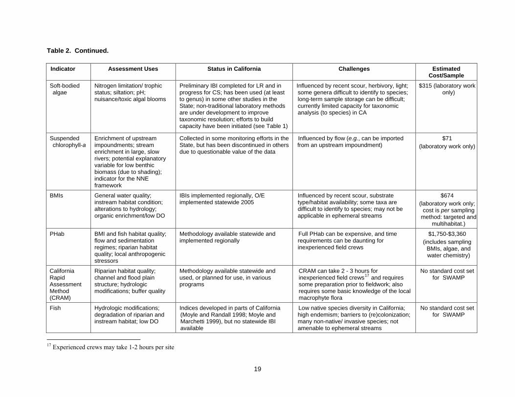
A number of issues related to bioindicator development and implementation are presented below, followed by recommendations for approaches and further applied research. Potential Indicators: Pros and Cons Developing and testing tools for bioassessment is a time-consuming and relatively expensive process. Decisions about how to invest limited dollars in development should involve a consideration of the benefits and challenges associated with potential indicators. Table 2 provides an overview of several types of indicators that could be used (or are already used, at least to some extent) in the State, along with the strengths of each, and some of the challenges and costs associated with their implementation. In the section that follows, technical issues specific to the various types of algal indicators are discussed in more depth.

Table 2. Comparison of algal and other indicators used, or under development, in California.

Indicator Assessment Uses Status in California Challenges Estimated Cost/Sample

(FY2007/2008)12

Chlorophyll a (from benthic and floating algae)

Stream productivity measured as abundance of microalgae13 (+ macroalgae14); key indicator for the NNE framework

Sampled in LR and CS; has been used in several types of studies throughout State; will be sampled for PSA; sampling methods not standardized – recommended for funding to standardize sampling approach

Influenced by recent scour, herbivory, light; content varies between species and within species depending on light and nutrients; may be difficult to draw conclusions based on these confounding factors

$71 (laboratory work

only)

Ash-free dry mass, AFDM (from benthic and floating algae)

Stream productivity measured as biomass of biofilm (+ macroalgae); key indicator for the NNE framework

Sampled in LR and CS; has been used in several types of studies throughout State; will be sampled for PSA; sampling methods not standardized – recommended for funding to standardize sampling approach (can co-occur with development of chlorophyll-a sampling standardization)

Influenced by recent scour, herbivory, light; confounded with non-algal organic matter (exacerbated with inclusion of depositional samples)

$43 (laboratory work

only)

Reach-wide algal percent cover

Amount of algae (microalgae + macrofilaments + floating mats) in the stream reach

Sampled in CS; conducted with a gridded viewing bucket, or as point-intercept concomitant with conducting PHab pebble counts – the latter is recommended

Difficult to assess in deep and/or swift and/or highly turbid streams

Included in PHab data collection, if part of pebble count

Diatoms Trophic status; organic enrichment; low DO; siltation; pH; metals

Preliminary IBI completed for LR15 and in progress for CS; has been used in some other studies in the State; efforts to build capacity have been initiated (see Table 1)

Influenced by recent scour, herbivory, light; may require SEM16 for some species and subspecies-level determinations; currently limited capacity for taxonomic analysis in CA

$315 (laboratory work only)

12 Values in boldface type are based on the list of prices for SWAMP program in the fiscal year 2007/2008 13 Microscopic, benthic algae that coat the surface of substrata 14 The macroalgal component of stream algae is not always included in sampling. 15 LR = Region 6 (where the preliminary algae IBI was developed, for the Lahontan Region); CS = Regions 3, 4, 9, and coastal part of Region 8 (corresponding to the current algae IBI-development projects underway on California’s central coast and in coastal southern California) 16 SEM = Scanning Electron Microscope

18

19

Table 2. Continued.

Indicator Assessment Uses Status in California Challenges Estimated Cost/Sample

Soft-bodied algae

Nitrogen limitation/ trophic status; siltation; pH; nuisance/toxic algal blooms

Preliminary IBI completed for LR and in progress for CS; has been used (at least to genus) in some other studies in the State; non-traditional laboratory methods are under development to improve taxonomic resolution; efforts to build capacity have been initiated (see Table 1)

Influenced by recent scour, herbivory, light; some genera difficult to identify to species; long-term sample storage can be difficult; currently limited capacity for taxonomic analysis (to species) in CA

$315 (laboratory work only)

Suspended chlorophyll-a

Enrichment of upstream impoundments; stream enrichment in large, slow rivers; potential explanatory variable for low benthic biomass (due to shading); indicator for the NNE framework

Collected in some monitoring efforts in the State, but has been discontinued in others due to questionable value of the data

Influenced by flow (e.g., can be imported from an upstream impoundment)

$71 (laboratory work only)

BMIs General water quality; instream habitat condition; alterations to hydrology; organic enrichment/low DO

IBIs implemented regionally, O/E implemented statewide 2005

Influenced by recent scour, substrate type/habitat availability; some taxa are difficult to identify to species; may not be applicable in ephemeral streams

$674 (laboratory work only;

cost is per sampling method: targeted and

multihabitat.)

PHab BMI and fish habitat quality; flow and sedimentation regimes; riparian habitat quality; local anthropogenic stressors

Methodology available statewide and implemented regionally

Full PHab can be expensive, and time requirements can be daunting for inexperienced field crews

$1,750-$3,360 (includes sampling

BMIs, algae, and water chemistry)

California Rapid Assessment Method (CRAM)

Riparian habitat quality; channel and flood plain structure; hydrologic modifications; buffer quality

Methodology available statewide and used, or planned for use, in various programs

CRAM can take 2 - 3 hours for inexperienced field crews17 and requires some preparation prior to fieldwork; also requires some basic knowledge of the local macrophyte flora

No standard cost set for SWAMP

Fish Hydrologic modifications; degradation of riparian and instream habitat; low DO

Indices developed in parts of California (Moyle and Randall 1998; Moyle and Marchetti 1999), but no statewide IBI available

Low native species diversity in California; high endemism; barriers to (re)colonization; many non-native/ invasive species; not amenable to ephemeral streams

No standard cost set for SWAMP

17 Experienced crews may take 1-2 hours per site

Types and Applications of Algal Indicators Measurement of biomass Indicators commonly used to measure algal biomass, and therefore productivity, in streams include chlorophyll-a, a photosynthetic pigment, and AFDM, which corresponds to the organic content of a given sample. Chlorophyll-a is determined by homogenizing the sample and extracting the chlorophyll from solid matter using acetone, then using photometric methods to detect the amount of chlorophyll-a. AFDM is determined by obtaining the total dry weight of a sample, combusting the sample to incinerate all the organic matter, and then reweighing the sample to determine its remaining ash content. The difference in weight before and after combustion represents the AFDM. Because it is presumed that algae comprise at least some portion of the sample, AFDM is considered to serve as an approximation of algal biomass (Steinman and Lamberti 1996). Algal abundance in a given reach, and therefore results for both types of biomass indicator, can be limited by nutrients (Francoeur 2001) and light (Hill 1996) and reduced by recent scour (Scrimgeour and Winterbourn 1989, Peterson 1996) and herbivory (Steinman 1996). Because of these potential confounding factors, it can be difficult to interpret the results of these assays. In addition, technical issues specific to chlorophyll-a include the fact that it can vary among different species of algae and can even vary within a species (e.g., as a function of exposure to light; Hill 1996). Furthermore, the method for AFDM is not selective for algae, and therefore other organisms such as bacteria, protozoans, and fungi can contribute to the AFDM measurement, as can fine organic debris from decaying leaves and wood (Steinman and Lamberti 1996). Programs in some states and countries have elected not to assess chlorophyll-a or AFDM because of uncertainty about the value of these measurements, not only because of confounding influences by various factors, but sometimes also because of dissatisfaction with the level of repeatability realized with these measures (Appendix A). Despite some technical issues that can present challenges to interpretation of biomass results, these indicators are very attractive for several reasons. The processes to collect and analyze biomass samples are relatively inexpensive and straightforward, and therefore reasonably accessible to a wide array of practitioners to address different assessment needs. In addition to this, measurements of chlorophyll-a and AFDM lend themselves well to assessments of beneficial uses thresholds that have been proposed (Dodds et al. 1998, Biggs 2000). Furthermore, various studies have indicated utility of these measures for assessment of biomass in relation to factors such as nutrient enrichment and/or surrounding land uses (Biggs 2000, Berkman and Porter 2004, Lavoie et al. 2004, Busse et al. 2006). Given some of the difficulties inherent in interpreting chlorophyll-a and AFDM, it is helpful to collect both types of data, and assess them in conjunction with one another for estimating biomass (Stevenson 1996). Collection of both types of biomass data also facilitates determination of the “autotrophic index,” which is calculated as the ratio of AFDM to chlorophyll-a and reflects the autotrophic component of the biomass contained in the sample (Collins and Weber 1978). If the benthic flora shifts to a more heterotrophic community in response to organic enrichment, the index value is expected to increase. Biggs (1989) found a strong relationship between the autotrophic index and biological oxygen demand. Moreover, from the standpoint of the California NNE, the ratio of the biomass values improves the

20

predictive capability of modeling tools for determination of nutrient numeric targets (Tetra Tech 2006). It should be noted that it is also beneficial to collect information on ambient parameters that may be influencing these biomass measures so that they can be evaluated in light of such factors. These parameters are discussed below. In addition to the quantitative laboratory methods described above to estimate algal biomass, techniques exist for assessing algal cover that are carried out entirely in the field. Cover estimates of algae, in terms of biofilms coating substrates, and attached filaments and floating mats, can be collected using gridded viewing buckets placed at specific points along a stream reach (EPA Rapid Bioassessment Protocol; Stevenson and Bahls in Barbour et al. 1999). Alternatively, during the course of conducting the pebble count that is part of the PHab portion of the SWAMP Bioassessment protocol (Ode 2007), algal abundance can be assessed via a point-intercept method by noting, for each piece of substrate where a sampling point falls, whether or not a “microalgal” layer is present, and if present, how thick the layer is. This approach has been used in NAWQA sampling (J. Berkman, pers. comm.) It can also be noted whether the sampling point falls onto macroalgae (e.g., in the form of attached filamentous algae or an unattached floating mat). These data can be compiled to provide a profile of the extent of algal cover in different strata within the steam. The field protocol used by the Southern and Central California IBI development projects incorporates this approach to algal-cover assessment (Appendix C). It should be noted that a more comprehensive assessment of reachwide algal biomass would require information about the thickness of the algal filaments and mats. This is difficult to measure in a meaningful way, because the mats vary in terms of density, thus obscuring thickness. Furthermore, it is not always clear what stratum a given algal specimen belongs to and therefore current methods still require some refinement. Despite these drawbacks, algal percent cover is an attractive approach to estimating productivity within a stream reach, because it involves a reasonably simple procedure that can economically be incorporated into existing SWAMP biomonitoring activities. Furthermore, thresholds for impacts to beneficial uses have been proposed for this parameter (Biggs 2000), and studies have indicated its utility in assessments of the effects of anthropogenic influences on algal nuisance (Busse et al. 2006, Busse 2007, Tetra Tech 2007). It is recommended that chlorophyll-a, AFDM, and algal percent cover assessment be included in SWAMP monitoring, and that biomass of detached, floating macroalgae (when present) be analyzed separately from attached/benthic, at least for the initial stages of developing the algae bioassessment program. We recommend that SWAMP fund an evaluation of the results of these initial assessments when sufficient data are available, in order to determine whether there is substantial value in continuing to collect each of the types of biomass data, and that protocols be refined and standardized for statewide use. Choice of algal assemblage In biomonitoring that involves assessment of algal assemblage, sometimes only benthic diatoms are used, and in other cases, soft-bodied algae are also included. Data collected for this latter assemblage may include only macroalgal forms, which are filaments and mats that we can easily see in the stream, or it may also include the “microalgal” coating on stream substrata.

21

While diatom communities have a history of extensive use for bioassessment in various parts of the world (Appendix B), and much has been accomplished to establish them as bioindicators (Round 1991, van Dam et al. 1994, Kelly and Whitton 1995, Stoermer and Smol 1999), opinions are more variable about the utility of soft-bodied algae assemblages, and they are not always included in algae-based bioassessment efforts. Furthermore, in at least one published case, soft-bodied algae were included but deemed, in retrospect, not to merit the extra effort (Lavoie et al. 2004). SWAMP will need to evaluate whether soft-bodied algal data provide sufficient information, beyond that which is provided by diatoms, in order to determine whether to continue to monitoring this assemblage over the long term. The preliminary algal IBI for the eastern Sierra Nevada (Herbst and Blinn 2007) utilizes both diatoms and soft-bodied algae; also, EMAP and NAWQA have both included this assemblage in their monitoring efforts. Of all the states surveyed that use algal assemblage measures as a component of their bioassessment programs, nearly half of them assess taxonomic composition of both diatoms and soft-bodied algae (Appendix A), and soft-bodied algae are also included in algae bioassessment efforts carried out in New Zealand and some parts of Europe (Appendix B). The remainder of states and countries surveyed use diatoms only, and none use soft-bodied microalgae alone in algal assemblage assessments. Some of the reasons for not including soft-bodied algae are based on laboratory considerations, and are discussed below. Because approaches exist for collecting soft-bodied algae concurrently with diatoms, there is minimal additional effort necessary in the field portion of the work in order to sample this assemblage18, and there are several reasons to include it in biomonitoring. From a biomass perspective, soft-bodied taxa are often the major component of the algal community in a given stream (Wehr and Sheath 2003), so to ignore them is to tell only part of the story about stream algae and productivity. Stevenson and Bahls (1999) recommend inclusion of soft-bodied algae because some impacts of interest may selectively affect, or be derivative of, this assemblage. For instance, soft-bodied algae (including cyanobacteria) are involved in toxic blooms (Baker et al. 2001, Izaguirre et al. 2007), and are frequently implicated in water taste and/or odor problems (Watson and Ridal 2004; reviewed by Jüttner and Watson 2007). However, Stevenson and Bahls (1999) also recommend that, if only one of the two assemblages can be assessed (due to financial constraints, for instance), diatoms should be chosen, because the diatom component of a given sample tends to be more species-rich and many metrics are based on differences in taxonomic composition. Herbst and Blinn (2007) found soft-bodied algae to provide a useful signal, and included a metric based on this assemblage (i.e., density of Stigeoclonium species) in their Eastern Sierra Nevada preliminary IBI. Other investigators have also found soft-bodied algae to be valuable indicators, particularly in relation to their responsiveness to nutrients (Douterelo et al. 2004, Berkman and Porter 2004, Parikh et al. 2006, Vis et al. 2008), and Foerster et al. (2004) were able to define reference stream classes in Germany based entirely on soft-bodied algal assemblages. Autecological information has been generated for many taxa in this assemblage (Leland and Porter 2000, Leland et al. 2001, Potapova 2005, Porter et al. 2008) and soft-bodied algal metrics 18 Additional effort involves collection of supplemental “qualitative” samples of macroalgae to assist in laboratory determinations.

22

have been included in a number of IBIs (e.g., Hill et al. 2000, Griffith et al. 2005, Herbst and Blinn 2007). Metrics exist for percent nitrogen fixers and percent seston19 in microalgae; both of these indicator types are largely represented by soft-bodied algae. Percent nitrogen-fixers can be used to identify sites with low nitrogen conditions, while increases in percent seston are useful in evaluating general stream condition in low-gradient agricultural areas. An advantage of these metrics is that they do not rely on species-specific information, further contributing to the attractiveness of soft-bodied algae as an indicator (J. Berkman, pers. comm.). The TAC recommends that both diatom and soft-bodied algal assemblages be included in SWAMP monitoring, at least for the initial stages of developing the State’s algal bioassessment program. The results from the first cycles of SWAMP/PSA algal monitoring, along with data from the Lahontan and Central and Southern California IBI development projects, should be used for an evaluation of the cost/benefit of continuing to assess both indicators. Laboratory and taxonomic issues There are a number of reasons why soft-bodied algae are not always included in bioassessment programs. For one thing, inclusion of this assemblage roughly doubles the laboratory labor associated with taxonomic analysis per site. Soft-bodied algae are more difficult than diatoms to preserve and store over long periods. They can also be more difficult to identify to species, and some taxa can be identified down to this level only if they happened to be in a sexual stage at the time of collection and fixation (Biggs 2000, Wehr and Sheath 2003), or if live material can be cultured in the laboratory and successfully induced into a sexual stage. Finally, soft-bodied algae can be challenging to enumerate when conducting quantitative assessment of the assemblage via commonly used approaches (e.g., Stevenson and Bahls 1999). However, an approach is currently being employed in southern California that addresses some of these issues. The time and expertise needed for species-level identification of algal taxa (both diatoms and soft-bodied algae) has compelled some investigators to examine the value of genus-level taxonomic information for assessment purposes. The appeal of an index using genus-level information is not only in that it reduces analysis time, but it could be much more accessible for application in lower-budget efforts like citizen’s watershed monitoring groups. Various investigators have created general pollution-assessment indices based on diatom genus-level taxonomic information (Rumeau and Coste 1988 and Coste and Ayphassorho 1991, both cited in Stevenson and Smol 2003). Hill et al. (2001) demonstrated that diatom assemblage attributes based on species- as well as genus-level sensitivity and tolerance values were “consistently and reliably related to gradients of human disturbance within a catchment.” However, the relative value of genus-level metrics was a function of the types of metrics used. For instance, when looking at attributes such as abundance of eutraphentic and pollution-tolerant diatoms, correlations between the calculated values at the genus and the species levels were weak, and the investigators concluded that a “significant loss of information” was realized when restricting identification to genus.

19 Suspended fine particulate material that can include planktonic algae.

23

Despite the potential appeal of genus-level metrics, many investigators have cautioned against such an approach (Round 1991) because of existence of sometimes-large ecological differences among congeners (Stevenson and Bahls 1999). Some have also cited intraspecific differences in autecologies as a reason to err toward taxonomic “splitting” rather than “lumping.” Potapova and Charles (2007) have suggested that some common species of diatom may actually constitute a group of multiple, indistinguishable de facto species or ecotypes. This was based on the discovery of differences in reported autecological characteristics for each of the species in question in different parts of the world. They therefore recommended erring toward more refined taxonomic treatment rather than lumping similar-looking taxa into morphospecies. As revealed in the lessons learned from other states surveyed (Appendix A), taxonomic congruence is a crucial element of an effective biomonitoring program. The TAC therefore recommends that SWAMP support the activities of an algal taxonomic workgroup, after the fashion of SAFIT, in order to foster the highest-quality taxonomic information possible for the implementation of algae bioassessment in the State. The main focus of this workgroup should be a standard algal taxonomic effort and it should include periodic workshops and development and maintenance of a webpage. The standard taxonomic information from algal assemblages, as well as all other biological data, should be stored together in the SWAMP database. Products of the taxonomic workgroup should include a standard taxonomic list and a standard taxonomic effort document. A preliminary workgroup has already been initiated through the southern California and central coast algal IBI-development projects. It is recommended that SWAMP take advantage of the opportunity to leverage this initial effort to build an algal taxonomy forum that will exist beyond the term of these grants. The southern California IBI project team is also developing preliminary taxonomic support resources for end users, such as a regional flora for diatoms and soft-bodied algae, specimen photos, and taxonomic keys. It is therefore also recommended that SWAMP build upon these support materials to expand their applicability to the flora of the State as a whole. Sampling Issues Sampling design One of the highest-priority decisions to be made early in the process of implementing algae-based bioassessment is what sampling protocol(s) to use throughout the State. As with BMIs, there are two general approaches to collecting quantitative samples of algae: 1) targeted sampling, in which specific types of substratum are sampled separately (e.g., the USGS NAWQA quantitative protocols; Moulton et al. 2002), and 2) multihabitat/reachwide sampling, in which substrata are selected objectively, in proportion to their relative abundances within the stream reach (e.g., the USEPA EMAP protocol; Peck et al. 2006). In the latter approach, algae from any number of substrata (e.g., from cobbles, sand, gravel, concrete, etc.) may be collected and composited into a single sample. Each approach has its pros and cons, and the decision about the protocol(s) to use statewide will depend upon a consideration of these differences because here are tradeoffs associated with adopting either method for statewide monitoring.

24

In the case of targeted sampling, because no single habitat type is present in all wadeable streams in the State, certain streams could be left out of ambient assessments, or it may not be feasible to compare data between certain stream types (for which different sampling methods would have to be applied, based on targeted substrate types.) Another disadvantage of targeted sampling is the need for a different set of reference sites for each targeted substrate type. There is also a possibility that indices might have to be fine-tuned for the different substrata (but see the discussion about substrate affinities below). Finally, there could be a greater potential for error associated with sampling bias, because of the potential for subjectivity inherent in identifying the richest targeted habitat. The multihabitat/reachwide approach, on the other hand, would mean one method is used everywhere, which could allow for a single database and assessment methodology for all California sites, and could therefore facilitate comparison of sites across the State. Benefits include the fact that dischargers and/or consultants would need to know only one method, which would make it much easier for Water Board permit writers to incorporate bioassessments into permit requirements. An important statistical argument for using a multihabitat sampling approach is that, because the sampling points are assigned objectively, the resulting composite sample is representative of the stream reach. However, a problem with this method is the fact that sampling points may sometimes fall upon spots in the stream that cannot be sampled (e.g., deep pools). While algal taxa can have substrate affinities (Burkholder 1996), literature on the topic indicates that algal metrics can be developed that are not highly sensitive to the method of sample collection (Pan et al. 1996, Potapova and Charles 2005, and Weilhoefer and Pan 2007), or habitat type (Winter and Duthie 2000a, Fore 2002). This suggests that either method might be acceptable in terms of its ability to generate results that would be useful for our purposes. A pilot sampling-method comparison study is being conducted by the southern California algae IBI project team. Results of this study should provide some insight into the sensitivity of the metrics/IBI that will be developed to the sampling methods employed, at least in that region. In the interim, until the results of these studies are available, the TAC recommends that algae be collected by SWAMP using at least the multihabitat/reachwide approach. It is further recommended that SWAMP fund, as a high priority, a “calibration” study of the targeted vs. reachwide algae-sampling methods in the Lahontan Region (LR). This is where the first algae-based IBI in California was developed. The results of such a study would allow us to determine whether existing datasets from that region, based on materials collected using a targeted-sampling approach, are comparable to data collected using a multihabitat approach, and if not, what additional steps may be necessary to be able to combine these data. Funding and contracting for such a study should begin as soon as possible. It is also recommended that SWAMP fund studies to refine the index period for algae sampling; however, in the interim, sampling should be conducted concurrently with BMIs, and should occur at least 30 days after any large storm or flow event. Also with regard to sampling period, it should be recognized that there are periods in some parts of the State when access for sampling may be limited or precluded (e.g., periods of high snow and ice cover in the high Sierra, periods

25

of high spring runoff in all parts of the State), and these periods should be accounted for both when planning sampling events and in the course of data interpretation. Additional parameters to measure in the field A number of environmental parameters can influence benthic algal communities, and an understanding of the factors at play can enhance interpretation of algal biomass and assemblage results. For instance, high-velocity flows can scour the benthos and remove biomass from the stream (Scrimgeour and Winterbourn 1989, Peterson 1996). Shading by a riparian canopy, or by suspended matter in the water column, can limit the amount of light accessible to the streambed, therefore curtailing biomass accrual. This may also select for taxa that are more tolerant of low-light conditions (Hill 1996). The effects of environmental factors can also manifest themselves by virtue of the various growth forms of different taxa. For example, diatom taxa that grow on stalks, and filamentous algae, can form canopies over prostrate taxa (those appressed to the substrate) that occupy the biofilm understory. Such characteristics influence patterns of recolonization post-disturbance and community succession, and can also confer differential resistance to high-velocity flows/scour, vulnerability to herbivory, and exposure to light (Poff et al. 1990, Hill 1996, Peterson 1996, Steinman 1996). Important environmental indicators to assess in conjunction with the collection of algal samples include many of the same data already collected for the PHab component of standard SWAMP bioassessment (Ode 2007), such as flow habitats and flow velocity/discharge, canopy cover, and water depth and turbidity, which can shade the benthos (Hill 1996). Pebble count data are valuable because of the responsiveness of the benthic algal assemblage to siltation (indicated by percent fines), which can select for motile taxa that are able to migrate to the surface when buried. A higher proportion of such taxa could reflect higher reproduction because of competitive dominance of these “fugitive” taxa. The “siltation index” based on prevalence of motile taxa can be used as a metric (Bahls 1993). In the course of conducting the pebble count, information about reachwide algal percent cover can also be collected. Information about the BMI assemblage can be helpful to explain algae bioassessment results by providing an indicator of herbivore pressure in the system. For example, Hirst et al. (2002) found grazer abundance to be a significant predictor of diatom assemblage characteristics. Water-chemistry parameters, including turbidity, alkalinity, conductivity, nutrients (e.g., total nitrogen, nitrate, total phosphorus, orthosphosphate), pH, and DO (preferably diel), help in the interpretation of algal data. Water-column chlorophyll-a can provide a means of identifying potential eutrophication in larger slow-moving systems, or upstream impoundments (Wehr and Sheath 2003). It can also serve as a potential explanatory variable for low benthic algae biomass (due to shading of the benthos; Hill 1996). The importance of measuring this parameter may vary depending on location of the monitoring. For example, it is likely less important in shaded, high-gradient streams than in more open, lowland systems with surrounding agricultural land uses. It should be noted that some monitoring programs in the State measured this parameter historically, but have since eliminated it because it did not seem to provide sufficiently useful information (e.g., San Francisco Bay RWQCB monitoring efforts, San Gabriel River watershed monitoring program).

26

The TAC recommends measuring all of the parameters indicated above in bold to accompany algal bioassessment. Water-column chlorophyll-a, however, should be measured only in larger, slow-moving systems and those downstream of impoundments. Analytical Issues Assemblage data reduction and interpretation Various approaches can be used to summarize information about algal communities for bioassessment purposes; many are similar to those commonly used in BMI studies. A thorough discussion of analytical approaches is beyond the scope of this document, so the main focus of this section will be on basic aspects of IBI development and application. A preliminary algal IBI has already been developed for use in the eastern Sierra Nevada (Herbst and Blinn 2007), and additional algal IBIs are currently under development in coastal watersheds of central and southern California. It should be noted that in addition to the IBI a second, very different, analytical approach to site assessment will also be used by at least the central California study group: An algae-based analog of the River Invertebrate Prediction and Classification System (RIVPACS; Wright 1995). This latter approach has been successfully applied to algal data in a recent study by Mazor et al. 2006. RIVPACS employs a predictive model to assess the degree to which the assemblage at a given site reflects that which would be expected in the absence of anthropogenic influences. It is, however, still unclear how widely applicable this approach may be, and both approaches to utilization of biomonitoring data have their strengths and weakness, as discussed by Karr and Chu (2000) and by Norris and Hawkins (2000). Examples of metrics used in algal IBIs Algal IBIs consisting of metrics using diatoms only, or including information about soft-bodied algae, have been employed for bioassessment by numerous practitioners (Hill et al. 2000, Fore 2002, Fore and Grafe 2002, Hill et al. 2003, Griffith et al. 2005, Wang et al. 2005, Herbst and Blinn 2007). Stoermer and Smol (1999) define metrics as “attributes of assemblages that change in response to human alterations of watersheds.” As with BMI assemblages, there are many different classes of metric that can be used to describe the nature of the algal assemblage of interest. For example, some metrics address “guilds” that may describe the autecological20, or morphological, aspects of the various taxa that comprise the sample. Other metrics relate to the relative tolerance, sensitivity, or requirements of taxa with respect to specific water-quality parameters (such as DO or pH ranges), or to more general factors such as “general pollution,” eutrophication, or organic pollution. A substantial amount of autecological information for the more common diatom species has been generated by numerous investigators (e.g., Lowe 1974, Lange-Bertalot 1979, Bahls 1993, van Dam et al. 1994), and an increasing body of knowledge is being developed for soft-bodied algae as well (Leland and Porter 2000, Leland et al. 2001, Potapova 2005, Porter et al. 2008).

20 Refers to the ecological conditions under which the taxon in question is known to occur. This type of information is useful for bioassessment applications.

27

Several metrics have been developed for using algae as indicators of eutrophication and organic pollution. Examples include percent eutrophic taxa, percent nitrogen heterotrophs, and percent saprobic taxa (van Dam et al. 1994). Nitrogen heterotrophs can use, or even require, organic nitrogen, and therefore tend to increase in relative abundance with increasing organic enrichment. Prevalence of saprobic taxa is indicative of high organic matter and low oxygen conditions. As mentioned previously, percent nitrogen fixers (i.e., nitrogen-fixing cyanobacteria taxa + diatom taxa that have cyanobacterial endosymbionts) is indicative of stream nitrogen status (Berkman and Porter 2004), with higher values corresponding to more nitrogen-poor systems. Although algae are often recognized and utilized for their high value as indicators for trophic status and organic wastes, they also have applications for assessment of other pollutant classes. Several studies have identified toxic effects of certain metals to algal taxa (reviewed by Genter 1996), and others have demonstrated relationships between metals and benthic algal communities (Hill et al. 2000, Hirst et al. 2002, Ivorra et al. 2002, Griffith et al. 2005). Hirst et al. (2002) generated a list of diatom species’ relative tolerances to metals based on results of their study. Diatoms can be particularly useful as indicators for metals, because at least some taxa can manifest the effects of metal stress through easily observed morphological deformations. This phenomenon forms a basis for the metric defined by percent aberrant diatoms (McFarland et al. 1997). The “siltation index” (Bahls 1993) is calculated based on the relative abundance of motile diatom taxa in the sample. When covered by sediment, individuals in these genera can migrate toward the surface. As such, higher values of this index correspond to increased siltation. The percent of live diatoms (Hill 1996) is reflective of health of the diatom assemblage, and can be used as an indicator for siltation. There are also diatom metrics more geared toward general water quality. These include the Pollution Tolerance Index (PTI; Kentucky DEP 2002), which is based on pollution-tolerance values assigned to diatom taxa. This index is calculated as the weighted average of the tolerance values represented by the taxa in the sample. Other examples are the Specific Polluosensitivity Index (SPI; Coste in CEMAGREF 1982) and the standardized Biological Diatom Index (BDI; Lenoir and Coste 1996). A software package called “Omnidia,” that was developed in France, is available for calculation of these and other diatom indices (Lecointe et al. 1993). It should be noted that, while it can be useful to conduct exploratory analyses using taxon-specific autecological information that has been developed in other regions, there may be a need for local fine-tuning as these values may vary geographically (Potapova and Charles 2007). It is anticipated that the algal data that have and will be generated throughout the State will form the basis of a database that can be used to begin validating/determining autecologies of the taxa by region. Once a surplus of metrics has been calculated using the taxonomic data, the metrics are screened according to a variety of criteria that reflect their potential utility for bioassessment purposes. Examples of screening criteria include how well the metrics correlate with measures of disturbance, their signal-to-noise ratios, the degree to which they are redundant with other metrics, and whether a given metric’s calculated values cover a range of values sufficient to be

28

useful for discriminatory purposes (Fore 2003). After a suite of viable metrics has been selected, they can be aggregated into multimetric indices for testing of index responsiveness to disturbance and selection of a final set of the appropriate number of metrics to comprise the index. Reference sites There are many factors capable of influencing stream algal communities that are not necessarily related to anthropogenic stress. These can include geologic setting (Biggs 1996, Stevenson 1997), which in turn can influence hardness, conductivity, and alkalinity (Foerster et al. 2004). Stream physical attributes relating to canopy cover, slope, and stream order can also come into play (Mazor et al. 2006). It will be important for a statewide program to determine how such factors influence algal communities in California, and what allowances will need to be made, perhaps in addition to what is required for BMIs, in order to define and utilize reference sites. The European Union’s Water Framework Directive (WFD) provides an example of defining criteria for a reference-site network that is sensitive to the biota used for monitoring. It requires that stream types be classified in order to facilitate the comparison of “apples to apples” when evaluating monitoring results vis-à-vis reference expectations. To fulfill this requirement for monitoring activities in Germany, Foerster et al. (2004) empirically defined three types of rivers and streams based on benthic algal assemblage information: 1) organic sites (influenced by peat), and 2) siliceous and 3) calcareous sites (influenced by basin geology). Foerster et al. (2004) found that, even among stream reaches that are essentially unimpacted by human activities, stream type was a significant determinant of algal assemblage. Without this kind of knowledge it would be difficult to establish whether deviations of algal assemblage taxonomic composition among assessed reaches were attributable to human activities alone, or natural variation in parameters unrelated to anthropogenic stress. Atmospheric deposition of nitrogen is also a potential concern in reference-site identification, at least for stream algae. It has been shown to contribute to nitrogen loading of streams in certain parts in the state (Fenn and Poth 1999) and may influence the algal flora even in otherwise “reference”-quality reaches in undeveloped catchments. Atmospheric deposition is likely to be most important in the vicinity of major metropolitan areas (such as the Los Angeles Basin). While modeling and on-the-ground deposition assessment can be used to identify hotspots of deposition, knowledge of the extent and magnitude of this phenomenon throughout the state is still limited. An interesting advantage of using diatoms for bioassessment is the amenability of this assemblage to historical reconstruction. Diatom frustules21 can remain well preserved over time, facilitating taxonomic identification even after cells die and their contents decompose. Diatoms on herbarium macrophyte specimens have been used to reconstruct the diatom assemblage of certain streams prior to major anthropogenic impacts (van Dam and Mertens 1993), thus providing insights into expected assemblage composition under reference conditions. In Canada, diatoms in the stomach contents of museum fish specimens are now being used for this same

21 The siliceous covering of a diatom cell.

29

purpose (I. Lavoie, pers. comm.). Techniques such as these may become increasingly important as true reference streams, particularly in certain landscapes, become rarer. Ode and Schiff (2008) recently drafted a Reference Condition Management Plan (RCMP) for California streams. Algal bioassessment in the State should take advantage of this effort to the greatest extent possible for opportunities to coordinate reference site selection and utilization with BMI and other bioassessment. Reference sites will need to be identified that cover the range of values of parameters found to influence algal assemblages under natural conditions. Sites should be classified in a way that allows comparison of monitoring reaches to reference reaches within the same class, allowing the signal of response to anthropogenic factors to be distinguished from background variation. Work toward development of a reference network for algae should include research that uses existing and newly generated datasets to establish patterns of occurrence of taxa across important chemical and physical gradients within the variety of reference reach settings that occur across the State. As the stream algal flora of the western United States becomes better defined through ongoing research and monitoring efforts in California and neighboring states, the nature of communities in pristine and minimally impacted reaches will come into focus. Partnerships should be formed with scientists in institutions in the State that study atmospheric deposition of nitrogen (e.g., the US Forest Service) in order to begin understanding where this phenomenon could most likely influence algal communities in reference reaches. Finally, other techniques, such as historical reconstruction of algal assemblages, should be undertaken for stream types for which it is now difficult to understand what reference conditions were like prior to human influences, such as low-gradient, high order systems.

30

INTEGRATION WITH OTHER BIOMONITORING DATA

SWAMP will eventually need to determine whether to assess all potential bioindicators at every site, or customize a suite of assessment tools on a case-by-case basis. It will also be necessary to determine how to integrate algae data with other types of data being collected, such as BMIs, PHab, and water chemistry. Complementarity of Bioindicators – Responses to Stress Selection of bioindicators depends on the goals of the assessment and the stressor type being assessed (Sonneman et al. 2001, Fore 2003, Hering et al. 2006, Newall et al 2006). Johnson and Hering (2004) acknowledge that, of BMIs, diatoms, macrophytes, and fish, the various assemblages can provide somewhat redundant information, and not all need to be assessed in every monitoring circumstance. They provide suggestions about which assemblages to monitor depending on the goal(s) of the monitoring (e.g., surveillance monitoring, operational monitoring, or investigations of catchment land-use effects) and the type of stream. Hering et al. (2006) stated that, of the four assemblages, diatoms were most responsive to eutrophication and nutrients. Diatoms also responded most strongly to land-use gradient, but it was suggested that this could be attributed, at least in part, to differences in life histories between the various assemblages. Hering et al. (2006) stated that, of the four above-mentioned assemblages if all cannot be used, then BMIs and benthic diatoms should be prioritized, because these assemblages are the most diverse and best reflect the major stress gradients. (It should be noted that soft-bodied algae were not considered in their assessment.) They further stated that, in small (European) mountain streams, fish assemblages were usually too species-poor, thus limiting the ability to construct metrics able to detect stressors. They also found patchy distribution patterns to limit applicability of macrophytes in some systems. If the interest of the investigation is on nutrient enrichment, Hering et al. (2006) recommended that algae and/or macrophytes be used. If the focus is on organic pollution, then BMIs and/or fish should be used, because of their more direct responsiveness to low DO. In justifying the value of using multiple assemblages, Newall et al. (2006) provided the example of a nutrient-rich discharge entering a rural or urban stream with low physical/habitat quality. Under such a scenario, BMIs might not perform well above or below the discharge, but diatoms could likely still detect a water-quality difference, as they are less prone to yield a low index value based on habitat considerations. Another argument for using multiple assemblages was noted by Hirst et al. (2002), who included information about grazer abundance in analyses and found it to be a significant predictor of diatom assemblage characteristics, suggesting the importance of understanding interactions among biotic factors in interpreting monitoring results. Complementarity of Bioindicators – Varying Temporal Scales Temporal patterns of responsiveness to changes in the environment should influence the choice of bioindicator for different assessment needs. Johnson and Hering (2004) consider diatom communities to be “early warning indicators.” Fore (2003) found that most of the variance in diatom assemblage associated with repeat visits to a given site was between site visits within a

31

year, rather than year-to-year. The opposite was true for fish and BMIs. These differences were interpreted as arising from differences in life cycles, with diatoms’ being the shortest, in general. Rimet et al. (2005) determined that different diatom metrics can have different “integration intervals,” meaning they require different periods of time to show response to changes in the environment. These investigators took sandstone blocks colonized with diatoms from a set of streams subject to different levels of human influence and transferred them all to a reference site, for subsequent analysis at varying time intervals. Depending on the index, it took anywhere from under 40, to as long as 60, days for indices calculated for the assemblages on the transferred blocks to “equilibrate” to their new environments. Lavoie et al. (2008) found that the integration times for diatom assemblages could vary from less than one week to as much as five weeks, and found stream trophic state to be a significant determinant of integration time.

32

33

SUMMARY OF RECOMMENDATIONS

Below is a summary of recommended general guiding principles for the development and implementation of algal bioindicators for California:

• Develop algal indicators with the primary goal of application in ALU assessment. • Prioritize development for use in wadeable, perennial streams. • Ensure that the algal indicator tools developed are applicable throughout the State. • Coordinate with other SWAMP bioassessment components whenever possible, as well as

with other monitoring and assessment programs around the State. • Use results from the first cycles of State algal monitoring, along with data from recent

IBI development projects in the State, to evaluate the cost/benefit of continuing to assess the full suite of TAC-recommend algal indicators: taxonomic composition of diatom and soft-bodied algal assemblages, chlorophyll-a, ash-free dry mass, and algal percent cover.

• Use the multihabitat/reachwide method for algae collection at all sites and recommend its use by other monitoring programs. (Note: A method-calibration study that assesses compatibility between results from this method, and the targeted-habitat method is also recommended to be carried out in the Lahontan Region; see Table 3).

• Sample algae during spring/summer, concurrently with BMIs sampling, and waiting at least 30 days after any large storm/flow events. (Note: Research on optimal index periods, and frequency, for sampling algae in different ecoregions of the State is recommended; see Table 3).

Table 3 provides a breakdown of specific recommendations regarding the algal indicators to develop for SWAMP monitoring, how to begin implementing them, and some of the anticipated research needs to address as the program matures.

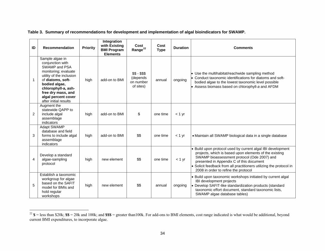
Table 3. Summary of recommendations for development and implementation of algal bioindicators for SWAMP.

ID Recommendation Priority Integration

with Existing BMI Program

Elements

Cost Range22

Cost Type Duration Comments

1

Sample algae in conjunction with SWAMP and PSA monitoring; evaluate utility of the inclusion of diatoms, soft-bodied algae, chlorophyll-a, ash-free dry mass, and algal percent cover after initial results

high add-on to BMI

$$ - $$$ (depends

on number of sites)

annual ongoing

• Use the multihabitat/reachwide sampling method • Conduct taxonomic identifications for diatoms and soft-

bodied algae to the lowest taxonomic level possible • Assess biomass based on chlorophyll-a and AFDM

2

Augment the statewide QAPP to include algal assemblage indicators

high add-on to BMI $ one time < 1 yr

3

Adapt SWAMP database and field forms to include algal assemblage indicators

high add-on to BMI $$ one time < 1 yr • Maintain all SWAMP biological data in a single database

4 Develop a standard algae-sampling protocol

high new element $$ one time < 1 yr

• Build upon protocol used by current algal IBI development projects, which is based upon elements of the existing SWAMP bioassessment protocol (Ode 2007) and presented in Appendix C of this document

• Solicit feedback from all practitioners utilizing the protocol in 2008 in order to refine the protocol

5

Establish a taxonomic workgroup for algae based on the SAFIT model for BMIs and hold regular workshops

high new element $$ annual ongoing

• Build upon taxonomic workshops initiated by current algal IBI development projects

• Develop SAFIT-like standardization products (standard taxonomic effort document, standard taxonomic lists, SWAMP algae database tables)

22 $ = less than $20k; $$ = 20k and 100k; and $$$ = greater than100k. For add-ons to BMI elements, cost range indicated is what would be additional, beyond current BMI expenditures, to incorporate algae.

34

Table 3. Continued.

ID Recommendation Priority Integration with

Existing BMI Program Elements

Cost Range23

Cost Type Duration Comments

6

Fund/conduct a method “calibration” study to determine compatibility of results from targeted and reachwide algae-sampling methods

high new element $$$ one time 1 - 2 years • Conduct the study in the Lahontan Region, where a

preliminary IBI has been developed based on data collected via targeted sampling

7

Fund/conduct research on optimal index periods, and frequency, for sampling algae in different ecoregions of the State

high new element $$$ one time 1 - 2 years • Build upon results of the pilot study initiated under the southern California IBI project

8

Identify a suite of reference sites statewide, including a definition of “stream types” if necessary (see Foerster et al. 2004)

medium add-on to BMI $$ one time 1 - 2 years • Coordinate with current Reference Condition Management Program (RCMP) efforts

9 Standardize laboratory protocols medium new element $ one time < 1 yr • Build upon protocols used by current algal IBI

development projects

10 Conduct field / taxonomy training workshops

medium new element $$ periodic ongoing • Build upon workshop materials created by current southern California algal IBI development project

11

Determine applicability of existing and soon-to-be-developed metrics/IBIs to statewide and/or appropriate ecoregional levels

medium new element $$ periodic ongoing • Can use algal data from PSA and SWAMP regional

monitoring (and other more local efforts, where applicable)

23 $ = less than $20k; $$ = 20k and 100k; and $$$ = greater than 100k. For add-ons to BMI elements, cost range indicated is what would be additional, beyond current BMI expenditure, to incorporate algae.

35

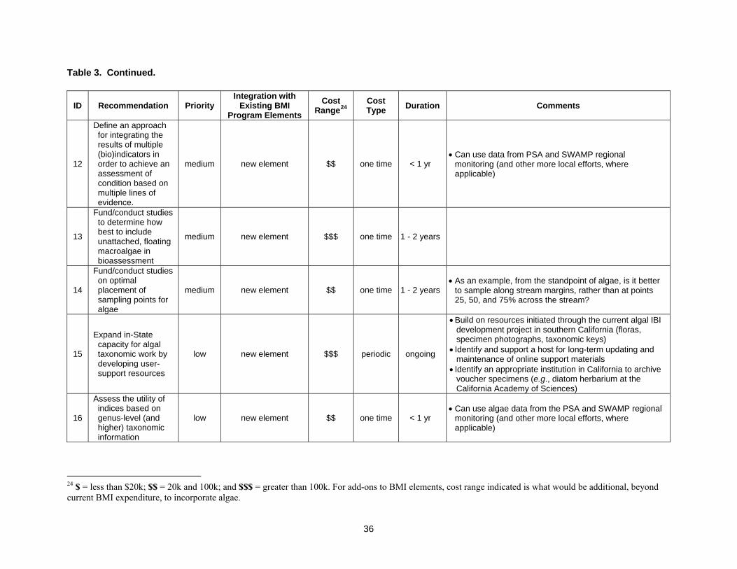
36

Table 3. Continued.

ID Recommendation Priority Integration with

Existing BMI Program Elements

Cost Range24

Cost Type Duration Comments

12

Define an approach for integrating the results of multiple (bio)indicators in order to achieve an assessment of condition based on multiple lines of evidence.

medium new element $$ one time < 1 yr • Can use data from PSA and SWAMP regional

monitoring (and other more local efforts, where applicable)

13

Fund/conduct studies to determine how best to include unattached, floating macroalgae in bioassessment

medium new element $$$ one time 1 - 2 years

14

Fund/conduct studies on optimal placement of sampling points for algae

medium new element $$ one time 1 - 2 years • As an example, from the standpoint of algae, is it better

to sample along stream margins, rather than at points 25, 50, and 75% across the stream?

15

Expand in-State capacity for algal taxonomic work by developing user-support resources

low new element $$$ periodic ongoing

• Build on resources initiated through the current algal IBI development project in southern California (floras, specimen photographs, taxonomic keys)

• Identify and support a host for long-term updating and maintenance of online support materials

• Identify an appropriate institution in California to archive voucher specimens (e.g., diatom herbarium at the California Academy of Sciences)

16

Assess the utility of indices based on genus-level (and higher) taxonomic information

low new element $$ one time < 1 yr • Can use algae data from the PSA and SWAMP regional

monitoring (and other more local efforts, where applicable)

24 $ = less than $20k; $$ = 20k and 100k; and $$$ = greater than 100k. For add-ons to BMI elements, cost range indicated is what would be additional, beyond current BMI expenditure, to incorporate algae.

Additional studies may be necessary in order to tailor bioassessment approaches for region-specific needs as algal bioassessment capability is developed statewide. These include research to address the following questions: • How do natural gradients in physical, chemical, and environmental aspects of California

streams influence algal monitoring results, and potentially our interpretation of the data? • Do algal assemblages in a specific reach respond more to local, or watershed-level

conditions? • Do different metrics/indices respond to factors at different spatial scales? • What were “reference” diatom communities like in lowland California streams prior to major

anthropogenic impacts? • On what time scale (e.g., days, weeks, months) do benthic algal assemblages shift in

response to changes in their environment (e.g., stressors)? • Is there utility in using artificial substrates for monitoring (e.g., to normalize across different

stream types that have different dominant substrata)?

37

REFERENCES Baker, P.D., D.A. Steffenson, A.R. Humpage, B.C. Nicholson, I.R. Falconer, B. Lanthois, K.M.

Fergusson and C.P. Saint. 2001. Preliminary evidence of toxicity associated with the benthic cyanobacterium Phormidium in South Australia. Environmental Toxicology 16:506-511.

Bahls, L.L. 1993. Periphyton bioassessment methods for Montana streams. Montana Water Quality Bureau, Department of Health and Environmental Science. Helena, MT.

Bain, M.B., J.T. Finn and H.E. Booke. 1988. Streamflow regulation and fish community structure. Ecology 69:382-392.

Barbour, M.T. and J.R. Karr. 1996. Biological Criteria: Technical Guidance for Streams and Small Rivers (revised edition) EPA-822-R-02-048. US Environmental Protection Agency. Washington, DC.

Barbour, M.T., J. Gerritsen, B.D. Snyder and J.B. Stribling. 1999. Rapid Bioassessment Protocols for Use in Streams and Wadeable Rivers: Periphyton, Benthic Macroinvertebrates and Fish. Second Edition. EPA 841-B-99-002. US Environmental Protection Agency, Office of Water. Washington, DC.

Barinova, S.S., M. Tavassi and E. Nevo. 2006. Algal indicator system of environmental variables in the Hadera River basin, central Israel. Plant Biosystems 140:65-79.

Berkman, J.A.H. and S.D. Porter. 2004. An overview of algal monitoring and research in the US Geological Survey’s National Water Quality Assessment (NAWQA) Program. Diatom 20:13-22.

Biggs, B.J.F. 1989. Biomonitoring of organic pollution using periphyton. South Branch, Canterbury, New Zealand. New Zealand Journal of Marine and Freshwater Research 23:263-274.

Biggs, B.J.F. 2000. New Zealand Periphyton Guideline: Detecting, Monitoring, and Managing Enrichment of Streams. New Zealand Ministry for the Environment. Christchurch, New Zealand.

Biggs, B.J.F. and C. Kilroy. 2000. Stream Periphyton Monitoring Manual. The New Zealand Ministry for the Environment, NIWA. Christchurch, New Zealand.

Borchardt, M.A. 1996. Nutrients. pp. 183-227 in: R.J. Stevenson, M.L. Bothwell and R.L. Lowe (eds.), Algal Ecology: Freshwater Benthic Systems. Academic Press. San Diego, CA.

Burkholder, J.M. 1996. Interactions of benthic algae with their substrata. pp. 253-297 in: R.J. Stevenson, M.L. Bothwell and R.L. Lowe (eds.), Algal Ecology: Freshwater Benthic Systems. Academic Press. San Diego, CA.

38

Burton, C.A., L.R. Brown and K. Belitz. 2005. Assessing water source and channel type as factors affecting benthic macroinvertebrate and periphyton assemblages in the highly urbanized Santa Ana River Basin, California. American Fisheries Society Symposium 47:239-262.

Burton, G.A., Jr., P.M Chapman and E.P Smith. 2002. Weight-of-evidence approaches for assessing ecosystem impairment. Human and Ecological Risk Assessment 8:1657-1673.

Busse, L.B., J.C. Simpson and S.D. Cooper. 2006. Relationships among nutrients, algae, and land use in urbanized southern California streams. Canadian Journal of Fisheries and Aquatic Sciences 63:2621-2638.

Busse, L.B. 2007. Algal nuisance in Rainbow Creek – Final Report. San Diego, CA.

Cairns, J., Jr., P.V. McCormick and B.R. Niederlehner. 1993. A proposed framework for developing indicators of ecosystem heath. Hydrobiologia 263:1-44.

CEMAGREF. 1982. Etude des methodes biologiques quantitatives d'appreciation de la qualite des eaux. Rapport Division Qualite des Eaux Lyon - Agence de l'Eau Rhone – Mediterranee - Corse, Pierre - Benite, 28 pp .

Chessman, B.C., N. Bate, P.A. Gell, and P. Newall. 2007. A diatom species index for bioassessment of Australian rivers. Marine and Freshwater Research 58:542–557.

Codd, G.A. 2000. Cyanobacterial toxins, the perception of water quality, and the prioritization

of eutrophication control. Ecological Engineering 16:51-60.

Cohen, P., W.M. Alley and W.G. Wilber. 1988. National Water-Quality Assessment: Future directions of the U.S. Geological Survey. Water Resources Bulletin 24:1147-1151.

Coleman, A.W. 1983. The roles of resting spores and akinetes in chlorophyte survival. pp. 1-21 in: Fryxel, G.A. (ed.), Survival Strategies of the Algae. Cambridge University Press. Cambridge, United Kingdom.

Collins, G.B. and C.T. Weber. 1978. Phycoperiphyton (algae) as indicators of water quality. Transactions of the American Microscopical Society 97:36-43.

Coste, M. and H. Ayphassorho. 1991. Étude de la qualité des eaux du Bassin Artois-Picardie à l’aide des communautés de diatomées benthiques (application des indices diatomiques). Rapport CEMAGREF. Bordeaux - Agence de l’Eau Artois-Picardie. Douai, France.

Davis, J.S. 1972. Survival records in the algae, and the survival role of certain algal pigments, fat, and mucilaginous substances. Biologist 45:52-93.

39

Dodds, W.K., J.R. Jones and E.B. Welch. 1998. Suggested classification of stream trophic state: distributions of temperate stream types by chlorophyll, total nitrogen, and phosphorus. Water Research 32:1455-1462.

Dodds, W.K., V.H. Smith and K. Lohman. 2002. Nitrogen and phosphorus relationships to benthic algal biomass in temperate streams. Canadian Journal of Fisheries and Aquatic Sciences 59:865-874.

Douterelo, I., E. Perona, and P. Mateo. 2004. Use of cyanobacteria to assess water quality in running waters. Environmental Pollution 127:377-384.

Feio, M.J., S.F.P. Almeida, S.C. Craveiro and A.J. Calado. 2007. Diatoms and macroinvertebrates provide consistent and complementary information on environmental quality. Fundamental and Applied Limnology/Archive für Hydrobiology 168:247-258.

Fenn, M.E. and M.A. Poth. 1999. Temporal and spatial trends in streamwater nitrate concentrations in the San Bernardino Mountains, Southern California. Journal of Environmental Quality 28:822-836.

Foerster, J., A. Gutowski and J. Schaumburg. 2004. Defining types of running waters in Germany using benthic algae: A prerequisite for monitoring according to the Water Framework Directive. Journal of Applied Phycology 16:407-418.

Fore, L.S. 2002. Response of diatom assemblages to human disturbance: Development and testing of a multimetric index for the Mid-Atlantic Region (USA). pp. 445-480 in: T.P. Simon (ed.), Biological Response Signatures: Indicator Patterns Using Aquatic Communities. CRC Press. Boca Raton, FL.

Fore, L.S. and C. Grafe. 2002. Using diatoms to assess the biological condition of large rivers in Idaho (U.S.A.). Freshwater Biology 47:2015-2037.

Fore, L.S. 2003. Developing biological indicators: Lessons learned from Mid-Atlantic streams. EPA 903/R-003/003. US Environmental Protection Agency, Office of Environmental Information and Mid-Atlantic Integrated Assessment Program, Region 3. Fort Meade, MD.

Francoeur, S.N. 2001. Meta-analysis of lotic nutrient amendment experiments: detecting and quantifying subtle responses. Journal of the North American Benthological Society 20:358-368.

Genter, R.B. 1996. Ecotoxicology of inorganic chemical stress. pp. 403-468 in: R.J. Stevenson, M.L. Bothwell and R.L. Lowe (eds.), Algal Ecology: Freshwater Benthic Systems. Academic Press. San Diego, CA.

Gomez, N. and M. Licursi. 2001. The Pampean Diatom Index (IDP) for assessment of rivers and streams in Argentina. Aquatic Ecology 35:173-181.

40

Griffith, M.B., B.H. Hill, F.H. McCormick, P.R. Kaufmann, A.T. Herlihy and A.R. Selle. 2005. Comparative application of indices of biotic integrity based on periphyton, macroinvertebrates, and fish to southern rocky Mountain streams. Ecological Indicators 5:117-136.

Gutowski, A. and J. Foerster. 2007. Benthische Algen ohne Kieselalgen und Armleuchteralgen – Feldführer. Landesamt für Natur, Umwelt und Verbraucherschutz Nordrhein Westfalen (LANUV NRW). Recklinghausen, Deutschland.

Herbst, D.B. and D.W. Blinn. 2007. Preliminary Index of Biological Integrity (IBI) for periphyton in the Lahontan Region, Eastern Sierra Nevada, California – Draft Report. Sacamento, CA.

Hering, D., R.K. Johnson, S. Kramm, S. Schmutz, K. Szoszkiewicz and P.F.M. Verdonshcot. 2006. Assessment of European stream with diatoms, macrophytes, macroinvertebrates and fish: a comparative metric-based analysis of organism response to stress. Freshwater Biology 51:1757-1785.

Hill, W. 1996. Effects of light. pp. 121-148 in: R.J. Stevenson, M.L. Bothwell and R.L. Lowe (eds.), Algal Ecology: Freshwater Benthic Systems. Academic Press. San Diego, CA.

Hill, B.H., A.T. Herlihy, P.R. Kaufmann, R.J. Stevenson, F.H. McCormick and C. Burch Johnson. 2000. Use of periphyton assemblage data as an index of biotic integrity. Journal of the North American Benthological Society 19: 50-67.

Hill, B.H., R.J. Stevenson, Y. Pan, A.T. Herlihy, P.R. Kaufmann, and C. Burch Johnson. 2001. Comparison of correlations between environmental characteristics and stream diatom assemblages characterized at genus and species levels. Journal of the North American Benthological Society 20:299-310.

Hill, B.H., A.T. Herlihy, P.R. Kaufmann, S.J. DeCelles, M.A. Vander Borgh. 2003. Assessment of streams of the eastern United States using a periphyton index of biotic integrity. Ecological Indicators 2:325-338.

Hirst, H.I., I. Jüttner and S.J. Ormerod. 2002. Comparing the responses of diatoms and macroinvertebrates to metals in upland streams of Wales and Cornwall. Freshwater Biology 47:1752-1765.

Ivorra, N., J. Hettelaar, M.H.S. Kraak, S. Sabater and W. Admiraal. 2002. Responses of biofilms to combined nutrient and metal exposure. Environmental toxicology and chemistry 21:626-632.

Izaguirre, G., A.D. Jungblut and B.A Neilan. 2007. Benthic cyanobacteria (Oscillatoriaceae) that produce microcystin-LR, isolated from four reservoirs in southern California. Water Research 41:492-498.

41

Johnson, R. and D. Hering. 2004. Standardisation of river classifications: Framework method for calibrating different biological survey results again ecological quality classifications to be developed for the Water Framework Directive. London, England.

Jowett, I.G. and B.J.F. Biggs. 1997. Flood and velocity effects on periphyton and silt accumulation in two New Zealand rivers. New Zealand Journal of Marine and Freshwater Research 31:287-300.

Jüttner, F. and S.B. Watson. 2007. Biochemical and Ecological Control of Geosmin and 2-Methylisoborneol in Source Waters. Applied and Environmental Microbiology 73:4395-4406.

Karr, JR. and E.W. Chu. 2000. Sustaining living rivers. Hydrobiologia 422/423:1-14.

Karr, J.R. 2006. Seven foundations of biological monitoring and assessment. Biologia Ambientale 20:7-18.

Kelly, M.G. and B.A. Whitton. 1995. The trophic diatom index: a new index for monitoring eutrophication in rivers. Journal of Applied Phycology 7:433-444.

Kentucky Department of Environmental Protection (DEP). Methods for assessing biological integrity of surface waters. Kentucky DEP, Division of Water, Ecological Support Section. Frankfort, KY.

Kingston, J.C. 2003. Araphid and monoraphid diatoms. pp. 595-636 in: J.D. Wehr and R.G. Sheath (eds.). Freshwater Algae of North America: Ecology and Classification. Academic Press. San Diego, CA.

Kolkwitz, R. and M. Marsson. 1908. Ecology of plant saprobia. [Translated 1967]. pp. 47–52 in: L.E. Keup, W.M. Ingram, and K.M. MacKenthum (eds.), Biology of Water Pollution. Federal Water Pollution Control Administration. Washington, DC.

Lange-Bertalot, H. 1979. Pollution tolerance of diatoms as a criterion for water quality estimation. Nova Hedwigia 64:285-304.

Lavoie, I., W.F. Vincent, R. Pienitz and J. Painchaud. 2004. Benthic algae as bioindicators of agricultural pollution in the stream and rivers of southern Quebec (Canada). Aquatic Ecosystem Health and Management Society 7:43-58.

Lavoie, I., S. Campeau, F. Darchambeau, G. Cabana and P.J. Dillon. 2008. Are diatoms good integrators of temporal variability in stream water quality? Freshwater Biology 53:827-841.

Lawrence, S.J. and R.L Seiler. 2002. Physical Data and Biological Data for Algae, Aquatic Invertebrates, and Fish from Selected Reaches on the Carson and Truckee Rivers, Nevada and California, 1993–97. US Geological Survey Open-File Report 02–012. USGS. Carson City, NV.

42

Lecointe, C., M. Coste and J. Prygiel. 1993. “Omnidia” software for taxonomy, calculation of diatom indices and inventories management. Hydrobiologia 269/270:509-513.

Leland, H.V. and S.D. Porter. 2000. Distribution of benthic algae in the upper Illinois River basin in relation to geology and land use. Freshwater Biology 44:279-301.

Leland, H.V., L.R. Brown and D.K. Mueller. 2001. Distribution of algae in the San Joaquin River, California, in relation to nutrient supply, salinity, and other environmental factors. Freshwater Biology 46:1139-1167.

Lembi, C.A. 2003. Control of nuisance algae. pp. 805-834 in: J.D. Wehr and R.G. Sheath (eds.), Freshwater Algae of North America: Ecology and Classification. Academic Press. San Diego, CA.

Lenoir, A. and M. Coste. 1996. Development of a practical diatom index of overall water quality applicable to the French National Water Board Network. pp. 29-43 in: B.A. Whitton and E. Rott (eds.), Use of Algae in Monitoring Rivers II. Institut für Botanik. Universität Innsbruck. Innsbruck, Austria.

Linthurst, R.A., L.A. Mulkey, M.W. Slimak, G.D. Veith and B.M. Levinson. 2000. Ecological research in the Office of Research and Development at the US Environmental Protection Agency: An overview of new directions. Environmental Toxicology and Chemistry 19:1222–1229.

Lobo, E.A., D. Bes, L. Tudesque and L. Ector. 2004a. Water quality assessment of the Pardinho River, RS, Brazil, using epilithic diatom assemblages and faecal coliforms as biological indicators. Vie Milieu 54:115-125.

Lobo, E.A., V.L.M. Callegaro, G. Hermany, N. Gomez and L. Ector. 2004b. Review of the use of microalgae in South America for monitoring rivers, with special reference to diatoms. Vie Milieu 54:105-114.

Lowe, R.L. 1974. Environmental Requirements and Pollution Tolerance of Freshwater Diatoms. EPA-670/4-74-005. US Environmental Protection Agency, National Environmental Research Center, Office of Research and Development. Cincinnati, OH.

Lowe, R.L. and Y. Pan. 1996. Benthic algal communities as biological monitors. pp. 705-739 in: R.J. Stevenson, M.L. Bothwell and R.L. Lowe (eds.), Algal Ecology: Freshwater Benthic Systems. Academic Press. San Diego, CA.

Lowe, R.L. 2003. Araphid and monoraphid diatoms. pp. 669-684 in: J.D. Wehr and R.G. Sheath (eds.). Freshwater Algae of North America: Ecology and Classification. Academic Press. San Diego, CA.

43

Mazor, R.D., T.B. Reynoldson, D.M. Rosenberg and V.H. Resh. 2006. Effects of biotic assemblage, classification, and assessment method on bioassessment performance. Canadian Journal of Fisheries and Aquatic Sciences 63:394-411.

McFarland, B.H., B.H. Hill and W.T. Willingham. 1997. Abnormal Fragilaria spp. (Bacillariophyceae) in streams impacted by mine drainage. Journal of Freshwater Ecology 12:141-149.

Moulton, S.R., II, J.G. Kennen, R.M. Goldstein and J.A. Hambrook. 2002. Revised protocols for sampling algal, invertebrate, and fish communities in the National Water-Quality Assessment program. U.S. Geological Survey Open-File Report 02-150. USGS. Reston, VA.

Moyle, P.B. and P.J. Randall. 1998. Evaluating the biotic integrity of watersheds in the Sierra Nevada, California. Conservation Biology 12:1318-1326.

Moyle, P.B. and M.P. Marchetti. 1999. Applications of indices of biotic integrity to California streams and watersheds. pp. 367-380 in: T.P. Simon and R. Hughes (eds.), Assessing the Sustainability and Biological Integrity of Water Resources Using Fish Communities. CRC Press. Boca Raton, FL.

Nandan, S.N. and N.H. Aher. 2005. Algal community used for assessment of water quality of Haranbaree dam and Mosam river of Maharashtra. Journal of Environmental Biology 26:223-227.

Newall, P., N. Bate and L. Metzeling. 2006. A comparison of diatom and macroinvertebrate classification of sites in the Kiewa River system, Australia. Hydrobiologia 572:131-149.

Norris R.H. and C.P. Hawkins. 2000. Monitoring river health. Hydrobiologia 435: 5-17.

Ode, P.R, A.C. Rehn and J.T. May. 2005. A quantitative tool for assessing the integrity of southern coastal California streams. Environmental Management 35:493-504.

Ode, P.R. and A.C. Rehn. 2005. Probabilistic assessment of the biotic condition of perennial streams and rivers in California. Report to the State Water Resources Control Board. California Department of Fish and Game Aquatic Bioassessment Laboratory. Rancho Cordova, CA.

Ode, P.R. 2007. Standard operating procedures for collecting macroinvertebrate samples and associated physical and chemical data for ambient bioassessments in California. California State Water Resources Control Board Surface Water Ambient Monitoring Program (SWAMP) Bioassessment SOP 001. State Water Resources Control Board. Sacramento, CA.

Ode, P.R. and K. Schiff. 2008. Recommendations for the development and maintenance of a reference condition management program (RCMP) to support biological assessment of

44

California’s wadeable streams. Southern California Coastal Water Research Project. Costa Mesa, CA.

Pan, Y. and R. Lowe. 1994. Independent and interactive effects of nutrients on benthic algae community structure. Hydrobiologia 291:201-209.

Pan, Y., R.J. Stevenson, B.H. Hill, A.T. Herlihy and G.B. Collins. 1996 Using diatoms as indicators of ecological conditions in lotic Systems: A regional assessment. Journal of the North American Benthological Society 15:481-495.

Parikh, A., V. Shah and D. Madamwar. 2006. Cyanobacterial flora from polluted industrial effluents. Environmental Monitoring and Assessment 116:91-102.

Peck, D.V., A.T. Herlihy, B.H. Hill, R.M. Hughes, P.R. Kaufmann, D. Klemm, J.M. Lazorchak, F.H. McCormick, S.A. Peterson, P.L. Ringold, T. Magee and M. Cappaert. 2006. Environmental Monitoring and Assessment Program-Surface Waters Western Pilot Study: Field Operations Manual for Wadeable Streams. EPA/620/R-06/003. US Environmental Protection Agency. Washington, DC.

Peterson, C.G. 1996. Response of algae to natural physical disturbance. pp. 375-402 in: R.J. Stevenson, M.L. Bothwell and R.L. Lowe (eds.), Algal Ecology: Freshwater Benthic Systems. Academic Press. San Diego, CA.

Pfister, P. and E. Pipp. 2007. Leitfaden zur Erhebung der Biologischen Qualitätselemente: Teil A3–Phytobenthos. Bundesministerium für Land- und Forstwirtschaft, Umwelt und Wasserwirtschaft, 89. Vienna, Austria.

Poff, N.L. N.J. Voelz and J.V. Ward. 1990. Algal colonization under four experimentally-controlled current regimes in a high mountain stream. Journal of the North American Benthological Society 9:303-318.

Ponander, K.C. and D.F Charles. 2004. Understanding the relationship between natural conditions and loadings on eutrophication: Algal indicators of eutrophication for New Jersey streams. Patrick Center for Environmental Research, Academy of Natural Sciences. Philadelphia, PA.

Porter, S.D., D.K. Mueller, N.E. Spahr, M.D. Munn and N.M. Dubrovsky. 2008. Efficacy of algal metrics for assessing nutrient and organic enrichment in flowing waters. Freshwater Biology 53:1036–1054.

Potapova, M. 2005. Relationships of soft-bodied algae to water-quality and habitat characteristics in U.S. rivers: Analysis of the NAWQA program data set. Report No. 05-08. Academy of Natural Sciences Patrick Center for Environmental Research – Phycology Section. Philadelphia, PA.

45

Potapova, M. and D.F. Charles. 2005. Choice of substrate in algae-based water-quality assessment. Journal of the North American Benthological Society 24:415-427.

Potapova, M.G. and D.F. Charles. 2007. Diatom metrics for monitoring eutrophication in rivers of the United States. Ecological Indicators 7: 48–70.

Prygiel, J. and M. Coste. 1993. The assessment of water quality in the Artois-Picardie water basin (France) by the use of diatom indices. Hydrobiologia 269/270:343-349.

Rankin, B. Miltner, C. Yoder and D. Mishne. 1999. Association between Nutrients, Habitat, and the Aquatic Biota in Ohio Rivers and Streams. Technical Bulletin MAS/1999-1-1; E. Ohio Environmental Protection Agency. Columbus, OH.

Rimet, F., H-M. Cauchie, L. Hoffman and L. Ector. 2005. Response of diatom indices to simulated water quality improvements in a river. Journal of Applied Phycology 17:119-128.

Robson, B. 2000. Role of residual biofilm in the recolonization of rocky intermittent streams by benthic algae. Marine and Freshwater Research 51:725-732.

Robson, B. and T. Matthews. 2004. Drought Refuges Affect Algal Recolonisation in Intermittent Streams. River Research and Applications 20:753–763.

Rott, E. 1991. Methodological aspects and perspectives in the use of periphyton for monitoring and protecting rivers. pp. 9-16 in: B.A. Whitton and E. Rott (eds.), Use of Algae in Monitoring Rivers II. Institut für Botanik, Universität Innsbruck. Innsbruck, Austria.

Round, F.E. 1991. Diatoms in river water-monitoring studies. Journal of Applied Phycology 3:129-145.

Rumeau, A. and M. Coste. 1988. Initiation a la systematique des Diatomees d'eau douce pour l'utilisation pratique d'un indice diatomique generique. Bulletin Francais de la peche et de la Pisciculture 309:1-69.

Schaumburg, J., U. Schmedtje, C. Schranz, B. Köpf, S.Schneider, P.Meilinger, G. Hofmann, A. Gutowski and J. Foerster. 2005. Instruction protocol for the ecological assessment of running waters for implementation of the EU Water Framework Directive: macrophytes and phytobenthos. Bavarian Water Management Agency. Munich, Germany.

Scrimgeour, G.J. and M.J. Winterbourn. 1989. Effects of floods on epilithon and benthic macroinvertebrate populations in an unstable New Zealand river. Hydrobiologia 171:33-44.

Shilling, F. 2005. Using periphyton in watershed assessment. in: F. Shilling (ed.), California Watershed Assessment Manual: Volume II. Prepared for the California Resources Agency and the California Bay-Delta Authority. Davis, CA.

46

Smith, E.P., I. Lipkovich and K. Ye. 2002. Weight-of-Evidence (WOE): Quantitative estimation of probability of impairment for individual and multiple lines of evidence. Human and Ecological Risk Assessment 8:1585-1596.

Soininen, J. and K. Könönen. 2004. Comparative study of monitoring South-Finnish rivers and streams using macroinvertebrate and benthic diatom community structure. Aquatic Ecology 38:63-75.

Sonneman, J.A., C.J. Walsh, P.F. Breen and A.K. Sharpe. 2001. Effects of urbanization on streams of the Melbourne region, Victoria, Australia. II. Benthic diatom communities. Freshwater Biology 46:553-565.

Steinman, A.D. 1996. Effects of grazers on freshwater benthic algae. pp. 341-373 in: R.J. Stevenson, M.L. Bothwell and R.L. Lowe (eds.), Algal Ecology: Freshwater Benthic Systems. Academic Press. San Diego, CA.

Steinman, A.D. and G.A. Lamberti. 1996. Biomass and pigments of benthic algae. pp. 295-313 in: F.R. Hauer and G.A. Lamberti (eds.), Methods in Stream Ecology. Academic Press. San Diego, CA.

Stevens, D.L., Jr. 1994. Implementation of a national environmental monitoring program. Journal of Environmental Management 42:1-29.

Stevenson, R.J. 1996. An introduction to algal ecology in freshwater benthic habitats. pp. 3-30 in: R.J. Stevenson, M.L. Bothwell and R.L. Lowe (eds.), Algal Ecology: Freshwater Benthic Systems. Academic Press. San Diego, CA.

Stevenson, R.J. 1997. Scale-dependent determinants and consequences of benthic algal heterogeneity. Journal of the North American Benthological Society 16:248-262.

Stevenson, R.J. and L.L. Bahls. 1999. Periphyton protocols. Chapter 6 in: M.T. Barbour, J. Gerritsen, B.D. Snyder, and J.B. Stribling (eds.), Rapid Bioassessment Protocols for use in Streams and Wadeable Rivers. Second Edition. EPA/841-B-99-002. US Environmental Protection Agency, Office of Water. Washington, DC.

Stevenson, R.J. and Y. Pan. 1999. Assessing environmental conditions in rivers and streams with diatoms. pp. 11-40 in: E.F. Stoermer and J.P. Smol (eds.), The Diatoms: Application for the Environmental and Earth Sciences. Cambridge University Press. Cambridge, United Kingdom.

Stevenson, R.J. and J.P. Smol. 2003. Use of algae in environmental assessments. pp. 775-804 in: J.D. Wehr and R.G. Sheath (eds.). Freshwater Algae of North America: Ecology and Classification. Academic Press. San Diego, CA.

Stoermer E.F. and J.P. Smol. 1999. The Diatoms: Application for the Environmental and Earth Sciences. Cambridge University Press. Cambridge, United Kingdom.

47

Taylor, J.C., W.R. Harding and C.G.M. Archibald. 2007. A methods manual for the collection, preparation and analysis of diatom samples. WRC Report TT 281/07. Water Research Commission Gezina. Pretoria, South Africa.

Tetra Tech. 2006. Technical Approach to Develop Nutrient Numeric Endpoints for California. Prepared for USEPA Region 9 and California State Water Resource Control Board. Tetra Tech, Inc. Lafayette, CA.

Tetra Tech. 2007. San Gabriel River Algae Study – Final Report. Tetra Tech, Inc. Lafayette, CA.

Tremp, H. and A. Kohler. 1995. The usefulness of macrophyte monitoring-systems, exemplified on eutrophication and acidification of running waters. Acta Botanica Gallica 142:541-550.

United State Environmental Protection Agency (USEPA). 2002. Methods for evaluating wetland condition: Using algae to assess environmental conditions in wetlands. EPA-822-R-02-021. US Environmental Protection Agency, Office of Water. Washington, DC.

van Dam, H. and A. Mertens. 1993. Diatoms on herbarium macrophytes as indicators for water quality. Hydrobiologia 269/270: 437-445

van Dam, H., A. Mertens and J. Sinkeldam. 1994. A coded checklist and ecological Indicator values of freshwater diatoms from The Netherlands. Netherlands Journal of Aquatic Ecology 28:117-133.

van den Hoek, C., D.G. Mann and H.M. Jahns. 1995. Algae: An Introduction to Phycology. Cambridge University Press. Cambridge, United Kingdom.

Vis, C., B. Upsdell, P. Chambers, D. McGoldrick, S. Jubeau, L-T. Pak, S. Sanchez, M. Souvignet and J. Wierdsma. 2007. Evaluation of various plant and dissolved oxygen metrics as indicators of eutrophication in agricultural watersheds in southern Ontario. National Agri-Environmental Standards Initiative Technical Series Report No. 3-51. Environment Canada. Gatineau, Quebec, Canada.

Vis., C., A. Cattaneo and C. Hudon. 2008. Shift from chlorophytes to cyanobacteria in benthic macroalgae along a gradient of nitrate depletion. Journal of Phycology 44:38-44.

Wang, Y-K., R.J. Stevenson and L. Metzmeier. 2005. Development and evaluation of a diatom-based Index of biotic Integrity for the Interior Plateau Ecoregion, USA. Journal of the North American Benthological Society 24:990-1008.

Watson, S.B. and J. Ridal. 2004. Periphyton: a primary source of widespread and severe taste and odour. Water Science and Technology 49:33-39.

48

Wehr, J.D. and R.G. Sheath. 2003. Freshwater habitats of algae. pp. 11-57 in: J.D. Wehr and R.G. Sheath (eds.). Freshwater Algae of North America: Ecology and Classification. Academic Press. San Diego, CA.

Weilhoefer, C.L. and Y. Pan. 2007. A comparison of diatom assemblages generated by two sampling protocols. Journal of the North American Benthological Society 26:308-318.

Winter, J.G. and H.C. Duthie. 2000a. Stream epilithic, epipelic and epiphytic diatoms: habitat fidelity and use in biomonitoring. Aquatic Ecology 34:345-353.

Winter, J.G. and H.C. Duthie. 2000b. Epilithic diatoms as indicators of stream total N and total P concentration. Journal of the North American Benthological Society 19:32-49.

Wright, J.F. 1995. Development and use of a system for predicting macroinvertebrate fauna in flowing waters. Australian Journal of Ecology 20:181-197.

49

APPENDIX A: SUMMARY OF ALGAL BIOASSESSMENT IN OTHER STATES

Introduction This appendix provides a summary of feedback from program directors and other staff involved in algae work in several other states in the U.S. The algae programs in these states are either currently being implemented (a minority of those surveyed) or are under development. The information was obtained in mid-to-late 2007 through interviews with staff members (generally via phone and email) and a review of pertinent documents and online resources. The states that currently have some form of algae bioassessment in progress, and for which information could be gathered for the present survey are: Alabama Alaska Arizona Delaware Florida Idaho Indiana Kentucky

Maine Massachusetts Missouri Montana New Jersey New Mexico New York Oklahoma

Pennsylvania South Dakota Tennessee Virginia West Virginia Wisconsin Wyoming

Most existing algae bioassessment programs, as well as those currently under development, aim to establish expectations for algae abundance and characteristics of the assemblage along a gradient of human disturbance. This gradient generally includes minimally disturbed reference sites as well as highly altered urban sites. The result is a taxonomic tolerance scale from which multiple metrics can be derived to establish a biological index using algae. While all state programs seek ultimately to utilize algal indices for stream monitoring, there are slight differences in approach from state to state. These differences can be categorized as follows:

• taxonomic focus • biomass assessment • percent cover assessment • sampling methodology • physical habitat assessment

A - 1

Taxonomic Focus Unless cost prohibitive, all states surveyed utilize diatoms in their algae biomonitoring programs, and a subset utilize both diatoms and soft-bodied algae. Diatoms are classified to the lowest possible level, typically species or variety, whereas soft-bodied algae are classified to family or genus. Diatoms are generally considered to be a more robust and consistent indicator of the integrity of the stream. Some respondents commented that soft-bodied algae seem to be more affected by confounding factors, which result in variability in abundance and taxonomic composition unrelated to anthropogenic disturbance. Because of this, some states have abandoned development of soft-bodied algae as an indicator. Those states that continue to pursue development of soft-bodied algae for bioassessment reasoned that it is too prevalent to be ignored. They are therefore taking steps to eliminate confounding factors. Budgetary constraints often dictate what data can be collected. As a result of insufficient funding, some states are unable to generate taxonomic data and are restricted to chlorophyll-a and/or density surveys. Table 1 shows the taxonomic focus of each state surveyed. Table 1. Taxonomic focus by state.

Diatoms Only Diatoms + Soft-bodied Algae

No Taxonomy (Chlorophyll or

Density only)

State AL, AZ, ID, MO, NJ, NM, NY, WV, WI

DE, FL, ME, MA, MT, PA, SD, VA, WY IN, OK, TN

Several states mentioned that they have experienced problems related to taxonomic inconsistencies between laboratories. To ameliorate this, the Phycology Section of the Patrick Center for Environmental Research at the Academy of Natural Sciences in Philadelphia is leading an effort to generate a national taxonomic guide and is providing taxonomic training to several state algae programs. Biomass assessment State algae programs are divided on the issue of how to assess algal biomass within a stream reach. The primary methods used are chlorophyll-a, ash-free dry mass (AFDM), or a combination of both. While many states collect biomass data, most reported that they are not seeing any significant correlation with their taxonomic metrics or with stream chemistry. Furthermore, the variability between duplicate samples is often large, which casts some doubt on the reliability of the measures. In addition, while chlorophyll-a is straightforward to collect from cobbles and other hard substrates, it is difficult to collect from fine-grained streams and the variability between duplicate samples in such systems is often so large as to make the values uninterruptible. As a result many states have abandoned the biomass assessments and others are considering abandoning it. Florida uses an assessment protocol that allows for the collection of both biomass and percent cover simultaneously. Their protocol lays out 99 points over a 100-meter reach. At each point

A - 2

they assess whether algae are present and the thickness of the mat at that location. Biomass assessment approaches for the various states are summarized in Table 2. Table 2. Biomass assessment by state. Chl a AFDM Chl a + AFDM Other None

State AL, MT, NM, NY, OK, WY WV, WI DE, IN, NJ, PA,

SD, VA, WV FL AZ, ID, KY, ME, TN

Percent Cover Assessment To assess percent cover of algae in a stream reach, most states are using either the Rapid Periphyton Survey, which creates visual estimates with the aid of a viewing bucket with 50-dot grid marked on the bottom (Stevenson and Bahls 1999), or a protocol that generates an estimate of percent cover by presence/absence at points along transects. Some of the RBP states are thinking of switching to the transect approach; however, this is considered to be more time-consuming and costly. Due to budgetary constraints, some states are only able to conduct a rough visual estimate in quartiles (0-25%, 25-50%, 50-75%, 75-100% cover) across the reach as a whole, and some are unable to collect percent cover data in any form. All states agreed that a more comprehensive and quantitative protocol would be more valuable. Table 3 provides a summary of the approaches used to assess algal percent cover by various states. Table 3. Percent cover assessment by state. RBP method

(viewing bucket)25Transects, point

intercept Rough Visual

Estimate None

State AL, KY, ME, NJ, OK, PA, TN, WI FL, NM, SD AZ, KY, MO, NY,

VA, WV, WY DE, ID, IN

Sampling Approach There are two basic approaches to collection of algae samples: targeted substrates, and reachwide/multihabitat. These methods are described in more detailed in the main body of this document. Of the algae programs that target a specific substrate, cobbles located in riffles and runs that have low canopy cover are the preferred substrate type for the states surveyed. Typically programs target cobbles, wood, and emergent plants in that order, which is congruent with the approach used by the USGS NAWQA Program (Moulton et al., 2002.) This particular set of substrates, which represent the “richest targeted habitat” for stream algae, is preferred for ease of comparability between sites that possess these habitats. Furthermore, cobbles in riffles are often the habitat targeted for benthic macroinvertebrate (BMI) sampling, so it is deemed efficient to send a single field team to assess both algae and BMIs. Such coordinated sampling is cost-effective and facilitates comparisons between the data sets. 25 Stevenson and Bahls 1999 in Barbour et al. 1999

A - 3

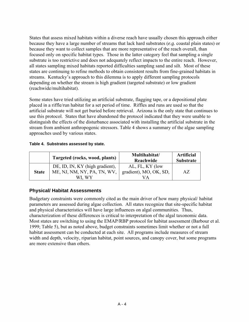
States that assess mixed habitats within a diverse reach have usually chosen this approach either because they have a large number of streams that lack hard substrates (e.g. coastal plain states) or because they want to collect samples that are more representative of the reach overall, than focused only on specific habitat types. Those in the latter category feel that sampling a single substrate is too restrictive and does not adequately reflect impacts to the entire reach. However, all states sampling mixed habitats reported difficulties sampling sand and silt. Most of these states are continuing to refine methods to obtain consistent results from fine-grained habitats in streams. Kentucky’s approach to this dilemma is to apply different sampling protocols depending on whether the stream is high gradient (targeted substrate) or low gradient (reachwide/multihabitat). Some states have tried utilizing an artificial substrate, flagging tape, or a depositional plate placed in a riffle/run habitat for a set period of time. Riffles and runs are used so that the artificial substrate will not get buried before retrieval. Arizona is the only state that continues to use this protocol. States that have abandoned the protocol indicated that they were unable to distinguish the effects of the disturbance associated with installing the artificial substrate in the stream from ambient anthropogenic stressors. Table 4 shows a summary of the algae sampling approaches used by various states. Table 4. Substrates assessed by state. Targeted (rocks, wood, plants) Multihabitat/

Reachwide Artificial Substrate

State DE, ID, IN, KY (high gradient), ME, NJ, NM, NY, PA, TN, WV,

WI, WY

AL, FL, KY (low gradient), MO, OK, SD,

VA AZ

Physical/ Habitat Assessments Budgetary constraints were commonly cited as the main driver of how many physical/ habitat parameters are assessed during algae collection. All states recognize that site-specific habitat and physical characteristics will have large influences on algal communities. Thus, characterization of these differences is critical to interpretation of the algal taxonomic data. Most states are switching to using the EMAP/RBP protocol for habitat assessment (Barbour et al. 1999; Table 5), but as noted above, budget constraints sometimes limit whether or not a full habitat assessment can be conducted at each site. All programs include measures of stream width and depth, velocity, riparian habitat, point sources, and canopy cover, but some programs are more extensive than others.

A - 4

Table 5. Types of physical/habitat assessments by state. Full Habitat Assessment* Limited Habitat Assessment+

State AL, FL, ID, KY, MO, NJ, NM, PA, SD, WV, WI, WY AZ, DE, IN, ME, OK, VA

*Full EMAP physical/habitat assessment +Limited EMAP: canopy cover, pebble counts, flow, stream width, depth, point sources only. Algae IBI Development Among the states surveyed, there were a variety of approaches to developing algal indices of biotic integrity (IBI), and many of the states surveyed are still very early in the process (Figure 1).

Pilot study/limited data

Early data analysis/Protocols established

SOPs set/ Developing IBI

Developed IBI

Routine Assessment

AL AZ DE FL ID IN KYMEMAMO NJNMNY OK PA SD TN VAWVWIWY Figure 1. Comparison of State’s progress in development and implementation of an algal IBI in their stream monitoring. The following section discusses the approaches of various states with respect to the following aspects of their algal index development efforts:

• Determination of reference conditions and/or gradients of human disturbance • Inclusion/exclusion of nonperennial streams • Coordinated sampling with other bioindicators • Linkages to nutrient criteria development, 303(d) listings, and TMDLs

A - 5

Reference Sites/ Gradients of Human Disturbance For most states, determination of reference sites is still largely based on best professional judgment. However, some states have begun development of statistical filters for a more quantitative and objective approach, and others are planning to follow suite. Most states are currently using watershed characteristics such as land-use, extent of hydrologic alteration, presence of discharges, and other human disturbances to identify reference locations. This is typically done using GIS layers that are verified in the field. Many states that have access to sufficient historical data are able to further refine reference site designations by assessing changes in stream chemistry and biological communities over time. Table 6 indicates how the various states identify reference sites. Table 6. Reference condition determination by state. Best Professional Judgment Statistical Filter None

State ID, IN, KY, ME, NJ, NM, PA, TN, WV, WI, WY

AL, AZ, FL, MO, VA

DE, NY, OK, SD

In addition to sampling streams across a gradient of human disturbance for algal index development, several states noted the importance of stratifying streams based on similarities in climate, habitat, geology, and geomorphology. Examples of classification strata include ecoregions, warm water vs. cold water, and gradient. Other factors used by some states when segregating streams for the purposes of data interpretation include the extent of light penetration, flow velocity/discharge, density of grazers, and water chemistry (dissolved oxygen, hardness, conductivity, and alkalinity.) Assessment of Nonperennial Streams While nonperennial streams represent a significant portion of stream miles in many states, most states have avoided sampling nonperennial streams due to the difficulties involved in distinguishing “natural” stresses due to seasonal dry periods from anthropogenic stresses. Of concern to the non-arid, eastern states, was the fact that it is difficult to define what is “intermittent.” Some streams may be dry in a drought year, but typically flow during other years. Nonperennial streams are considered a unique water body type and the main reason for not including these systems in bioassessment efforts is that there is no budget to develop an IBI for a second water body type. However, most of the arid states surveyed (MO, AZ, ID, WY, NM) recognize the importance of including nonperennial streams in bioassessment activities and hope to develop protocols for them in the future. Coordinated Sampling All states plan to coordinate algae collection with sampling for benthic macroinvertebrates, nutrient chemistry, and habitat assessment. Some will coordinate with fish collection as well. Most states envision having multiple indicators for nutrient criteria development, 303d listings,

A - 6

and TMDLs such that decisions for listings and remediation are firmly supported by the best available science. Nutrient Criteria All states surveyed plan to link algal bioassessment to nutrient criteria. However, most states are still in the early stages of this process, and actual “criteria” have not been set by any state. All states prefer to set thresholds at “biologically meaningful” values rather than percentiles, but determination of these thresholds is not anticipated in the near future. Most states have only conducted initial surveys and are still conducting their data analysis and establishing their IBIs. All states surveyed plan to utilize expert panels, statistical methods, and stakeholder input when establishing their algae nutrient criteria. Most states mentioned that they would use algae together with a habitat assessment, benthic macroinvertebrates, nutrient concentrations, and/or fish in a “weight of evidence” approach. 303(d) Listings and TMDLs Most states plan to use the algal bioassessment for 303(d) listing and TMDLs but they do not have enough data to support criteria for listings yet. However, a few states have expressed concern that algal metrics might not work consistently or with sufficient confidence. Summary of Lessons Learned One of the primary precautionary notes made by survey respondents related to the importance of taxonomic consistency. Different laboratories were sometimes found to produce significantly different results when examining the same sample. States agreed that there is a need to develop a universal taxonomy that everyone can use to expedite comparisons among states and regions. As a corollary to this, personnel need consistent training in identification. As a first step to resolving this issue, it was noted that the Philadelphia Academy of Sciences has taken the lead in offering training courses and developing taxonomies for several states. Several difficulties have been discovered with respect to common algae sampling approaches. For all these reasons, protocols in the states surveyed are continuously being refined and updated as new information becomes available.

• Many states noted that biomass measurements (chlorophyll-a and ash-free dry mass) are not producing consistent or highly useful results.

• Percent cover measurements do not seem to be very quantitative or consistent. • Artificial substrates have been found not to produce results consistent with human

disturbance or nutrient enrichment. • Sampling in shifting sandy- or silty-bottomed streams presents a challenge for algal

assessment, both in the field collection phase, and in the laboratory analysis phase. • There is some disagreement over whether sampling a targeted substrate or reach-wide is a

better approach. • Despite their potential relationship to nutrient enrichment, soft-bodied algae are not as

consistent an indicator as diatoms.

A - 7

Despite some shortcomings noted by respondents, algal assemblages are seen as a powerful tool, especially when combined with other bioindicators, such as macroinvertebrates and/or fish. Respondents felt that algal assemblages are most sensitive to stream chemistry, whereas fish are most sensitive to physical stress, and macroinvertebrates are sensitive to both chemistry and physical stress. Thus, the combination of indicators can be a very valuable for assessing stream condition and providing insights into the causes of impairment.

A - 8

REFERENCES Barbour, M.T., J. Gerritsen, B.D. Snyder and J.B. Stribling. 1999. Rapid Bioassessment

Protocols for Use in Streams and Wadeable Rivers: Periphyton, Benthic Macroinvertebrates and Fish. Second Edition. EPA 841-B-99-002. US Environmental Protection Agency, Office of Water. Washington, DC.

Moulton, S.R., II, J.G. Kennen, R.M. Goldstein and J.A. Hambrook. 2002. Revised protocols for sampling algal, invertebrate, and fish communities in the National Water-Quality Assessment program. U.S. Geological Survey Open-File Report 02-150. USGS. Reston, VA.

Stevenson, R.J. and L.L. Bahls. 1999. Periphyton protocols. Chapter 6 in: M.T. Barbour, J. Gerritsen, B.D. Snyder, and J.B. Stribling (eds.), Rapid Bioassessment Protocols for use in Streams and Wadeable Rivers. Second Edition. EPA/841-B-99-002. US Environmental Protection Agency, Office of Water. Washington, DC.

A - 9

APPENDIX B: SUMMARY OF ALGAL BIOASSESSMENT IN SELECTED

OTHER COUNTRIES

Bioassessment efforts incorporating algal indicators are undertaken in many parts of the world. In order to understand some of the motivations for algal bioassessment, approaches used, and insights gained through experiences of others, we conducted a survey of activities and programs in regions outside the United States. This appendix provides a summary of survey findings; it is not meant to be an exhaustive account of all applicable monitoring programs or efforts. European Union The history of utilization of benthic algae for water-quality assessment purposes goes back 100 years in Europe (Kolkwitz and Marsson 1908). The continued widespread application of algae in stream monitoring in many parts of Europe today testifies to the fact that algae remain highly valued as bioindicators. According to the European Union’s (EU) Water Framework Directive (WFD), all member countries are required to evaluate waters and meet WFD criteria, which include all water bodies achieving “good Ecological Status” by 2015. The WFD expressly includes “Composition and Abundance of Aquatic Flora” as “Quality Elements” to be used for the assessment of Ecological Status and potential in rivers and streams. “Flora” in their definition includes both macrophytes and benthic algae, and encompasses higher aquatic plants, mosses, and water ferns, as well as diatoms and cyanobacteria (WFD 2003). In order to best utilize algal indicators to facilitate monitoring per the WFD, some countries have developed detailed bioassessment protocols. These sometimes include supporting materials such as descriptions and pictures of algal taxa from the local floras (Schaumburg et al. 2005, Gutowski and Foerster 2007, Pfister and Pipp 2007). Approaches for integration of algae with other assemblages in biomonitoring (Johnson and Hering 2004, Pfister and Pipp 2007) have also been developed. Within the general guidelines of the WFD, different countries design and implement their own algal bioassessment programs. For instance, while most countries for which survey data were gathered regularly use taxonomic composition of diatom assemblages alone (e.g., Poland, Spain, Sweden, United Kingdom), a minority (e.g., Austria, Germany) also include soft-bodied algae. With respect to biomass, there appears to be a strong preference for estimation of percent cover (if anything) as opposed to analysis of chlorophyll-a and AFDM. None of the respondents reported regular use of the latter in their programs, but most assess percent cover in some manner. While an exhaustive survey of all algal biomonitoring programs in Europe is beyond the scope of this appendix, the program in Austria will be highlighted as an example of one country’s decisions about what to monitor and how, within the WFD framework. In Austria, the primary goals for the algal component of biomonitoring efforts are for assessing organic enrichment and nutrient impairment. Cobbles are considered the preferred substratum from which to sample, but if they are not present, then the sediment surface is sampled. While biomass measurement in terms of chlorophyll-a and AFDM are not included in the assessments, percent algal cover is estimated using a viewing bucket, as is thickness of microalgal layers on

B - 1

substrata. Both diatom and non-diatom algal assemblages (minus Charaphytes) are assessed, along with cyanobacteria. Taxonomic identifications are to species level, or as low as possible without having to use more involved techniques (such as scanning electron microscopy or culturing) for finer taxonomic resolution. Soft-bodied algal taxa and diatoms are given equal weight in analyses, and relative abundances of the taxa in each assemblage are determined. Three types of index are calculated from the algal assemblage data: 1.) tropic state, 2.) saprobic state, and 3.) observed/expected (O/E) taxa, using assemblages from reference sites for comparison. An Ecological Quality Ratio is calculated based on the worst performer of the three indices, and ultimately, a single value is derived based on the algae and other bioindicators. The WFD requires a comparison of the benthic algal assemblage of each monitored stream with a reference community from the same type of water body. To facilitate this, sites are stratified by physical and geographic variables (such as stream type, ecoregion, and elevation), and reference sites are identified within each stratum. The more “reference” species (and the fewer “tolerant” species) that are found in a given stream, the higher the assigned Ecological Status for that water body. Conversely, the greater the deviation of species composition in the assessed stream from reference assemblages, the more degraded it is deemed, and the lower the Ecological Status category assigned. As is the case with California, the issue of how to deal with sampling and interpreting data from intermittent streams is a major concern in the semi-arid region of Mediterranean Europe, which includes parts of Italy, France, Spain, Portugal, and Greece. However, no standardized approach has been developed to address any specials needs of intermittent systems. As such, they are sometimes excluded from bioassessment efforts. Lessons learned and recommendations from the European Union component of this survey include the following:

• Some respondents expressed the importance of identifying algal taxa to species whenever possible. It has been estimated that when ~30% or more of taxa cannot be identified to species, taxonomic resolution tends to be insufficient for use of the data in bioassessment analyses (Pfister and Pipp 2007).

• Sampling of algae should be conducted at the end of the dry season, and at least 30 days should be allowed to pass following the most recent storm.

• Assessment and reference sites should be stratified according to physical and geographic factors that can influence algal communities but are relatively insensitive to anthropogenic influences. This will provide a stronger signal to stressors above background variation.

In addition, Johnson and Hering (2004) made the following specific recommendations about using multiple assemblages for biomonitoring: • In small mountain streams, benthic diatoms (soft-bodied algae were not considered) should

be used for eutrophication and acidification effects, and BMIs for “various stressors”

B - 2

• In medium-sized mountain streams and lowland streams, benthic diatoms or macrophytes should be used for eutrophication and land-use effects, and BMIs or fish for hydromorphological and land-use effects

However, it was also noted that benthic diatoms and macrophytes might serve as good complementary indicators for nutrient enrichment, due to different temporal ranges, with diatoms serving as early-warning indicators and macrophytes as late-warning. The same would be true for using BMIs (which, depending on the taxon, could be considered either early- or late-warning) in conjunction with fish (late-warning) for hydromorphological and land-use effects. New Zealand Algae are an important component of biomonitoring activities in New Zealand pursuant to the Resource Management Act (RMA) of 1991, which states that the life-supporting capacity of the environment must be maintained, and that “there shall be no undesirable biological growths as a result of any discharge of a contaminant into water”. Major goals of the RMA include protection of aquatic ecosystem purposes, fish spawning, contact recreation, water supply, irrigation, and industrial abstraction. Because of the emphasis on control of nuisance algae to protect these uses, algal biomass is a cornerstone of many types of monitoring efforts in New Zealand; however other bioindicators are also employed, depending upon the goals of the assessment. These can include diatom and soft-bodied algal assemblages, as well BMIs and/or fish. Biggs (2000) produced a guideline document to help water managers with facilitating the intent of the RMA by determining human impacts on stream algae. This was accompanied by a comprehensive methods manual (Biggs and Kilroy 2000) that discusses a variety of assessment needs, such as ambient surveys or upstream-vs.-downstream monitoring at a point-source discharge point, and recommendations for the appropriate sampling method for each. While algae sampling in New Zealand generally focuses on targeted substrata, allowances are made for collections from either erosional (e.g., rock or macrophyte) habitats, or depositional areas (e.g., sand), and multihabitat sampling is even included in some bioassessment efforts. For routine assessments, algal percent cover and thickness are most commonly measured, while biomass analyses of chlorophyll-a are generally included only when there are issues of eutrophication. Some types of monitoring efforts, such as pre-development environmental impact assessments, often incorporate synoptic assessments of algal assemblage as well. When taxonomic enumerations are carried out, both diatoms and soft-bodied algae are considered, as the full complement of algal assemblage information is deemed much more informative for environmental resource decision-making than that of diatoms alone. Calculation of indices based on the taxonomic information is generally not undertaken due to the perception that a significant amount of information is lost in the data-reduction process. Rather, there is a tendency to use other ways of summarizing the data, such as basic graphing of results (B. Biggs, pers. comm.) Lessons learned in New Zealand include the recognition of a need for repeated sampling to give useful biomass results. While biomass has been found to serve as a good indicator for some questions, such data are perceived to be particularly valuable when a time series of samples is collected. Pooling of such samples for analysis has been found to provide valuable information

B - 3

while affording an economy of resources to help offset the need for large sample sizes over time (B. Biggs, pers. comm.) Canada While benthic algae are routinely monitored in some parts of Canada (such as the Province of Alberta), the assemblage is not currently used as standard bioindicator in any national water quality monitoring programs. It is, however, used as a eutrophication indicator in the development of nutrient standards. There is currently an effort to develop national (and regional) standards and sampling approaches to satisfy the goals of the National Agri-Environmental Standards Initiative (NAESI) which seeks, in part, to identify/validate robust and reliable bioindicators of stream trophic status. Studies have been conducted in recent years with the goal of providing guidance pursuant to the NAESI in terms of indicators of, and targets for, “aquatic plant” abundance, composition, or production that define trophic status of streams (Vis et al., 2007). Data collected have included cover of macrophytes and mosses, diatom species composition and soft-bodied algal genus composition, as well as biomass measurements. With respect to algae, cobbles have been targeted for taxonomic analysis as well as for determination of chlorophyll-a and AFDM, however, a multi-habitat approach has also been used for a semi-quantitative sampling of the soft-bodied algae. Several methods have also been piloted for assessing algal percent cover. Some of the lessons learned and recommendations that have been generated from the studies of Vis et al. (2007) are as follows:

• Since filamentous algal length was found to be correlated with total phosphorus and cover total nitrogen, the utility of metrics based on filamentous algae should be tested further in a larger number of streams

• Data on macroalgal genera should be combined with percent cover data to develop quantitative models and metrics of eutrophication.

• The effects of riparian zone vegetation on light availability should be considered when setting stream eutrophication guidelines.

• Benthic samples for biomass determination should be collected from both open and closed canopy areas within the same site.

South Africa The South African National Aquatic Ecosystem Monitoring Program (NAEMP) is multi-institutional in scope and has the overall goal of delivering “the ecological information for rivers and the broader aquatic ecosystems required to support the rational management of these systems”. The River Health Programme (RHP) that supports the NAEMP seeks to generate information required to report on the ecological state of South Africa’s river systems. Along with physical and chemical indicators, the RHP program has traditionally focused on the following bioindicators: 1) benthic macroinvertebrates, 2) fish, 3) riparian vegetation, and 4) habitat integrity. More recently, however, diatoms have been developed for inclusion into the suite.

B - 4

For the purposes of the RHP, diatoms are identified to species. The results are currently summarized in a generic biological diatom index, but development of a specific diatom index is currently underway. Data on algal biomass and percent cover are not included in the monitoring. Taylor et al. 2007 produced a methods manual for collection and analysis of diatom samples for bioassessment. While sampling is generally from cobbles in riffles or stems of vegetation, methods have been developed for sampling from other substrata, when necessary, such that all stream types can be included in assessment. Both perennial streams and intermittent streams are sampled for diatoms, however there are currently no special sampling or analytical methods in place that distinguish between the two stream types. With respect to lessons learned, investigators in South Africa expressed finding that genus-level information about diatom assemblages is of little if any value for bioassessment purposes, while species-level information is very powerful (W.R. Harding, pers. comm.) Other Countries Benthic algae have also been used in regional monitoring efforts and water-quality studies in many other nations, such as Israel (Barinova et al. 2006), India (Nandan and Aher 2005), Brazil (Lobo et al. 2004a,b), Argentina (Gomez and Licursi 2001, Lobo et al. 2004b), and Australia (Chessman et al. 2007).

B - 5

REFERENCES

Barinova, S.S., M. Tavassi and E. Nevo. 2006. Algal indicator system of environmental variables in the Hadera River basin, central Israel. Plant Biosystems 140:65-79.

Biggs, B.J.F. 2000. New Zealand Periphyton Guideline: Detecting, Monitoring, and Managing Enrichment of Streams. New Zealand Ministry for the Environment. Christchurch, New Zealand.

Biggs, B.J.F. and C. Kilroy. 2000. Stream Periphyton Monitoring Manual. The New Zealand Ministry for the Environment, NIWA. Christchurch, New Zealand.

Chessman, B.C., N. Bate, P.A. Gell, and P. Newall. 2007. A diatom species index for bioassessment of Australian rivers. Marine and Freshwater Research 58:542–557.

Gomez, N. and M. Licursi. 2001. The Pampean Diatom Index (IDP) for assessment of rivers

and streams in Argentina. Aquatic Ecology 35:173-181.

Gutowski, A. and J. Foerster. 2007. Benthische Algen ohne Kieselalgen und Armleuchteralgen – Feldführer. Landesamt für Natur, Umwelt und Verbraucherschutz Nordrhein Westfalen (LANUV NRW). Recklinghausen, Deutschland.

Johnson, R. and D. Hering. 2004. Standardisation of river classifications: Framework method for calibrating different biological survey results again ecological quality classifications to be developed for the Water Framework Directive. London, England.

Kolkwitz, R. and M. Marsson. 1908. Ecology of plant saprobia. [Translated 1967]. Pages 47–52 in L.E. Keup, W.M. Ingram, and K.M. MacKenthum, eds. Biology of water pollution. Federal Water Pollution Control Administration, Washington, DC.

Lobo, E.A., D. Bes, L. Tudesque and L. Ector. 2004a. Water quality assessment of the Pardinho

River, RS, Brazil, using epilithic diatom assemblages and faecal coliforms as biological indicators. Vie Milieu 54:115-125.

Lobo, E.A., V.L.M. Callegaro, G. Hermany, N. Gomez and L. Ector. 2004b. Review of the use of microalgae in South America for monitoring rivers, with special reference to diatoms. Vie Milieu 54:105-114.

Nandan, S.N. and N.H. Aher. 2005. Algal community used for assessment of water quality of Haranbaree dam and Mosam river of Maharashtra. Journal of Environmental Biology 26:223-227.

Pfister, P. and E. Pipp. 2007. Leitfaden zur Erhebung der Biologischen Qualitätselemente: Teil A3–Phytobenthos. Bundesministerium für Land- und Forstwirtschaft, Umwelt und Wasserwirtschaft, 89. Vienna, Austria.

B - 6

Schaumburg, J., U. Schmedtje, C. Schranz, B. Köpf, S.Schneider, P.Meilinger, G. Hofmann, A. Gutowski and J. Foerster. 2005. Instruction protocol for the ecological assessment of running waters for implementation of the EU Water Framework Directive: macrophytes and phytobenthos. Bavarian Water Management Agency. Munich, Germany.

Taylor, J.C., W.R. Harding and C.G.M. Archibald. 2007. A methods manual for the collection, preparation and analysis of diatom samples. WRC Report TT 281/07. Water Research Commission Gezina. Pretoria, South Africa.

Vis, C., B. Upsdell, P. Chambers, D. McGoldrick, S. Jubeau, L-T. Pak, S. Sanchez, M. Souvignet and J. Wierdsma. 2007. Evaluation of various plant and dissolved oxygen metrics as indicators of eutrophication in agricultural watersheds in southern Ontario. National Agri-Environmental Standards Initiative Technical Series Report No. 3-51. Environment Canada. Gatineau, QC, Canada.

Water Framework Directive (WFD). 2003. Overall Approach to the Classification of Ecological Status and Ecological Potential. Water Framework Directive Common Implementation Strategy Working Group 2 A Ecological Status (ECOSTAT).

B - 7

APPENDIX C: EXAMPLE OF A PROTOCOL FOR SAMPLING ALGAE

DRAFT

A Reachwide/Multihabitat Approach for Stream Algae and Associated Physical Habitat

Sample and Data Collection

Based on Elements from the Standard Operating Procedure

for SWAMP Bioassessment by Ode (2007)

May 2008

C - 1

Table of Contents List of Field Supplies - Algae Sample and PHab Data Collection ..................................... 3 1. Getting started ................................................................................................................ 5

1.1 Before Setting Out for the Field................................................................................ 5 1.2 Before Leaving Vehicle for Site ............................................................................... 5 1.3 Upon Arriving at the Site.......................................................................................... 5 1.4 Determining whether the site is appropriate for sampling........................................ 5

2. Preparing for Sample and Data Collection .................................................................... 6 2.1 Documenting the Reach............................................................................................ 6 2.2 Delineating the Study Reach..................................................................................... 6 2.3 Marking the Transects............................................................................................... 7 2.4 Notable Field Conditions .......................................................................................... 8

3. Algae Sample Collection................................................................................................. 9 3.1 Multihabitat Sample Collection ................................................................................ 9 3.2 Sample Processing .................................................................................................. 12 3.3 Qualitative Algae Sample Collection...................................................................... 15

4. PHab Transect-Based Measurements........................................................................... 17 4.1 Wetted Width .......................................................................................................... 17 4.2 Bankfull Width........................................................................................................ 17 4.3 Bankfull Height....................................................................................................... 17 4.4 “Pebble Count”: Transect Substrates ...................................................................... 18 4.5 Depth....................................................................................................................... 18 4.6 Particle Size Class................................................................................................... 18 4.7 Cobble Embeddedness ............................................................................................ 19 4.8 CPOM ..................................................................................................................... 20 4.9 Algal Cover............................................................................................................. 20 4.10 Dry Portions of Stream ......................................................................................... 22 4.11 Bank Stability........................................................................................................ 22 4.12 Human Influence................................................................................................... 22 4.13 Densiometer Readings (Canopy Cover) ............................................................... 23

5. PHab Inter-Transect-Based Measurements.................................................................. 25 5.1 Inter-transect Wetted Width.................................................................................... 25 5.2 Inter-transect Substrates and Algal Percent Cover ................................................. 25 5.3 Flow Habitats .......................................................................................................... 25 5.4 Photographs............................................................................................................. 26

6. Reachwide Measurements............................................................................................. 27 6.1 Gradient................................................................................................................... 27 6.2 Stream discharge..................................................................................................... 28

6.2.1 Discharge: Velocity Area Method ................................................................... 29 6.2.2 Discharge: Neutrally Buoyant Object Method ................................................ 30

7. References ..................................................................................................................... 32

C - 2

LIST OF FIELD SUPPLIES FOR ALGAE SAMPLE AND ASSOCIATED PHAB DATA COLLECTION

General

• Full sets of datasheets on Rite-in-the-Rain paper (including at least one spare set) • Fine-tipped and thick-tipped, waterproof pens • Clipboards (at least two) • Clipboard carriers (optional) • Site dossiers containing site maps, aerials, etc. • Thomas Guides and regional maps • Batteries (AA, 9-volt) • Ice chests with wet ice • Dry ice (if not returning to lab immediately following the day’s fieldwork) • First-aid kit • Cell phones • Sunscreen/hats/sunglasses • Bug repellant • Tecnu (for poison oak) • Snake chaps • Drinking water, snacks

Algae sample collection

• White washtub, rectangular, plastic • Composite sample receiving bottle, 1 L, plastic (one per site) • Graduated cylinder, 250 mL and 25 mL, plastic • PVC delimiter with 4-cm diameter • Spatula • Rubber delimiter with 4-cm diameter • Algae brushes (clean toothbrushes) • Syringe scrubber, 60 mL syringe barrel with end cut off and plunger fitted with Velcro • White (non-pigmented) scrubby pads cut to size for the syringe scrubber (several circles

per site) • Metric calipers • Scissors • Calculator • Snapping Petri dishes, 47 mm (2 per site) • Filter forceps • Glass fiber filters, 47 mm, 0.7 μm pore size (including foil-wrapped, pre-combusted

filters for AFDM) (2 of each type per site) • Filtering tower, 47 mm • Aluminum foil • Wash bottles • DI water

C - 3

• Hand vacuum pump • 25% glutaraldehyde solution (at least 10 mL per site) • Latex gloves, powder-free (at least 1 pair per site) • Razor blades or Swiss army knife • Turkey baster • Sample labels (4 per site) • Clear plastic tape (5 cm wide) • Centrifuge tubes, 50 mL, plastic (2 per site) • Whirl-pak bags, 100 mL (at least 2 per site) • Viewing bucket (gridded not necessary)

PHab data collection

• GPS receiver • Measuring tape • Lengths of rope (7.5 m and 12.5 m) • Small metric ruler (waterproof) • Digital watch and random number table • Digital camera • Stadia rod • Clinometer • Autolevel and tripod • Current velocity meter and top-setting rod • Convex spherical densiometer, taped to expose only 17 intersections of the grid • Transect flags, orange and yellow, labeled with transect and inter-transect names,

respectively • Rangefinder

C - 4

1. GETTING STARTED

1.1 Before Setting Out for the Field • Use the equipment checklist to make sure all necessary supplies are brought along. • Have in mind at least 3 sites to visit that day (target 2 and have another site in mind as a

back up if one of the first two sites is not useable.) • Check site dossiers to make sure they are complete with maps/directions to sites and

aerial photo. Bring along county maps, atlases, and Thomas Guides to further aid location of sites. Also bring along any site access permits, passes, and/or keys, as needed.

1.2 Before Leaving Vehicle for Site Make sure car is parked in a safe spot and there are no “No Parking” signs. Stick a business card with cell phone number in the driver’s window. Be sure to display the brown administrative pass placard if you are on National Forest land (or the letter of permission that is in your site dossier, if applicable). 1.3 Upon Arriving at the Site Your site dossier contains maps, an aerial photograph, and in some cases, a USGS quad sheet, all of which indicate the approximate location of the area of stream intended for our assessment. These coordinate may come from previous monitoring efforts where investigators may have taken GPS readings in adjacent parking lots or from nearby roads or bridges, or using a GPS unit with poor reception/low accuracy. Because of this, they may not have a very high level of accuracy, and should not be interpreted literally. If you are conducting a repeat visit at a site where data were collected previously for this project, your dossier should contain an aerial with the upstream and downstream transect locations indicated so that you may return to them and collect from the same area collected from previously. Site photos of transects A and K should also be included to assist identification of upstream and downstream limits of the reach. Finally, coordinates corresponding to transects A and K should be pre-programmed into the GPS. 1.4 Determining whether the site is appropriate for sampling Once the site has been located, make an initial survey of the reach from the stream banks (being sure to not disturb the instream habitat). Ensure that there is sufficient flowing water along the length of the reach of interest to collect water samples and algae. If there is insufficient water, document this, but do not use this site for the study at this time. Before leaving, take some photographs of the site, and fill out information on the Site Reconnaissance datasheet. This site may be suitable for use during a subsequent sampling period if there is water in the channel at some later date. The information recorded will be useful for determining whether the site may be of interest for incorporation into the study at that time.

C - 5

2. PREPARING FOR SAMPLE AND DATA COLLECTION

It is imperative that you confirm throughout the data collection effort at each site that all necessary data have been recorded correctly, by double-checking values, and confirming spoken values with your partner(s). As a general practice, you should conduct a final check across all datasheets that there are no missing values before you leave the site, and rectify any blanks.

2.1 Documenting the Reach If the site is deemed useable for the day of the visit, fill out the Reach Documentation section of the field forms. Determine the geographic coordinates of the downstream or upstream end of the reach (wherever you’re at at that time) with a GPS set for the NAD83 datum. Record in decimal degrees to five decimal places. Note: Later, once you have established all your transects, you will also record the coordinates for the other end of the reach. Be aware that some GPS units re-set themselves to factory default settings when the batteries are changed. This can include the datum. Therefore, anytime you remove batteries from your unit, double check that the unit is still using the NAD83 datum once the batteries are replaced.

2.2 Delineating the Study Reach Staying out of the channel, you’ll need to scout the study reach in its entirety in order to make sure that it is of adequate length for our purposes (150m or 250m-long26.) Conversely, if the reach cannot be that long (for reasons stated below), you’ll need to determine the useable length of the reach, and how to space your transects so that you can fit in 11 of them at equal distances from one to the next. Start out a little bit outside of what you anticipate will be the outer boundary of the reach (based on aerials and maps), count at least 150 large paces (for most adults, a large step is roughly equal to a meter.) Note what average wetted width27 appears to be. If the average wetted width is ≤ 10 m, you will end up using a 150-m study reach for your data collection. If the average wetted width is > 10 m, you’ll use a 250-m reach length. You can either estimate this by eye as you go along, or make your determination by a few taking cross-sectional width measurements at a locations along the way that are “representative” of the reach at large. However, if you choose the latter method, try to avoid stepping into the water in the channel as you pull the tape measure across the channel. Only cross where there are rocks or other emergent objects you can walk upon. 26 The standard sampling layout consists of a 150-m reach (length measured along the bank) divided into 11 equidistant transects that are arranged perpendicularly to the direction of flow. Ten additional transects (designated “inter-transects” here) located between the main transects give a total of 21 transects per reach. Main transects are designated A through K while inter-transects are designated by their nearest upstream and downstream transects (e.g., AB, BC, etc.). “A” is the downstream most transect. In extreme circumstances, reach length can be shorter than 150 m (e.g., if upstream and downstream barriers preclude a 150-m reach), but this should be avoided whenever possible. Streams > 10 m wetted width should use a reach length of 250 m. If the actual reach length is other than 150 m or 250 m this should be noted and explained on the field forms. This approach is based on the guidance for SWAMP bioassessment collection of Physical Habitat data (Ode 2007.) 27 Wetted Width~ The wetted channel is the zone that is inundated with water and the wetted width is the distance between the sides of the channel at the point where substrates are no longer surrounded by surface water. Measure the wetted stream width and record this in the box at the top of each transect form.

C - 6

A study reach should be free of any hydrologic inputs that could potentially modify the water-chemistry environment across the reach. Thus, there should be no tributaries or “end-of-pipe” outfalls feeding into the channel along the study reach. Look for any such features along the banks as you are pacing off the reach length, and if any occur, decide whether to define the reach as occurring entirely above or entirely below that feature. Alternatively, if you encounter such a feature when you have nearly reached the 150m (or 250m) target length of your study reach, then record what the current pace count is, and use that as your study reach length. Divide the paced reach length by 20. This will be the distance between the alternating adjacent Main, and Inter-, transects. Other features that should also not be present within a study reach are: bridge crossings, changes between natural and man-made (i.e., concrete) channel bottoms, waterfalls, impoundments (dams and weirs), etc. Whatever your study reach length turns out to be (150m, 250m, or other), record it on the datasheet under “Reach Length.” 2.3 Marking the Transects Once you have determined that the study site will provide a reach of adequate length, record the upstream or downstream GPS point (depending on where you are when you start out) and include it on the datasheet under “Reach Documentation”. Put down an orange flag at water’s edge on one of the banks to indicate the first “Main Transect”. Establish the positions of the remaining transects by heading along the entire length of the study reach (again, staying out of the water/channel as much as possible) and using the segment of rope of appropriate length to measure off successive segments of 7.5 m (for streams of wetted width ≤ 10 m), or 12.5 m (for streams > 10 m wetted width), or use the tape measure for whatever alternative length you calculated, based your measured study-reach length (see above). As you measure, always follow the curvature, or sinuosity, of the stream channel, not the water’s edge”, which may be irregular, and not reflective of the true stream linear footage. Estimate transect positions (and where on the banks to place the flags) by visually projecting perpendicularly from the mid-channel to the banks. (Refer to Figure 1 for a visual clarification of transect alignment relative to the stream’s direction of flow.) At the end of each measured segment as you head along the stream, mark the transect location on the bank with flag. Alternate between two different flag colors (orange will correspond to “Main Transects”, and yellow to “Intertransects”.) When you have finished, the downstream-most flag will correspond to Main Transect “A”, and the upstream-most flag (the 21st in the entire series of Main and Inter- transects) will correspond to Main Transect “K”.

C - 7

Figure 1. Reach layout geometry for physical habitat and biological sampling showing positions of 11 main transects (A – K) and the 10 supplemental inter-transects (AB- JK). The area highlighted in the figure is expanded in Figure 8. Note: reach length = 150 m for streams ≤ 10-m average wetted width, and reach length = 250 m for streams > 10-m average wetted width. 2.4 Notable Field Conditions Record under “Notable Field Conditions” any evidence of recent flooding, fire, or other disturbances that might influence algae samples. Especially note if flow conditions have been affected by recent rainfall, which can cause significant under-sampling of algae biomass and diversity. If you are unaware of recent fire or rainfall events, select the “no” option on the forms. Record the dominant land use and land cover in the area surrounding the reach by evaluating land cover within 50 m of either side of the stream reach. You can use your scaled aerial photograph of the site and vicinity to guide you. (Note that a yellow line corresponding to 150m has been drawn on the aerial photograph for each site roughly along a portion of the stream. This can be used to give the assessors a rough idea of scale of the aerial, which is useful for scoring several of the field parameters.)

C - 8

3. ALGAE SAMPLE COLLECTION

Algae should be collected from each transect prior to PHab data collection, so as not to disturb the algae by “trampling” the transects before the samples are collected. Furthermore, to avoid disturbing the transects for the collection of PHab data, collect algae at a distance of 1 m downstream of each transect. Algae (and PHab) data collection begins at Transect A and proceeds upstream to Transect K. This protocol focuses on collection of algae from multiple habitats composited into one sample. This “reachwide” method seeks to sample from the variety of microhabitats that exist in the stream reach, in proportion to which those microhabitats occur. For this method, we use as guidance the approach followed by EPA’s Environmental Monitoring and Assessment Program (EMAP; Peck, et al., 2006.) The “multihabitat” procedure for algae collection employs an objective method for selecting subsampling locations that is built upon the 11 Main Transects used for benthic macroinvertebrate collection and PHab measurements in SWAMP bioassessment (Ode 2007.). This procedure can be used to sample any wadeable stream reach, since it does not target specific habitats. Because sampling locations are defined by the transect layout, the position of individual sub-samples may fall within a variety of “erosional” or “depositional” habitats. For the multihabitat method, the sampling position within each transect is alternated between the left, center, and right positions along a transect (defined as the points at 25%, 50% and 75% of wetted width, respectively) as you move upstream from transect to transect. Starting with the downstream transect (Transect A), identify a point that is 25% of the stream width from the left bank (as you are facing downstream). Note: The actual sampling location should be displaced one meter downstream of the Main Transects in order to avoid disturbing substrates for subsequent PHab assessments. During algae collection and processing, make every attempt to keep the sample material out of the sun as much as possible. Try to do most or all work in the shade, and process samples as quickly as possible, because chlorophyll a begins to degrade when exposed to light. Also, before you begin sampling at any given site, make sure that the washtub has been very carefully cleaned since the last site, so that no algal material is carried over to contaminate the current sample. The same applies to all other algae collection apparati (brushes for scrubbing, graduated cylinder, turkey baster, PVC and rubber delimiters, spatulas, syringe scrubber, etc.) 3.1 Multihabitat Sample Collection Step 1: 1) Starting with Transect A, determine whether the selected sampling point is located in an erosional (e.g., riffle) habitat or a depositional (slack-water, pool) habitat. Based on this, collect a single sample at the point using the appropriate procedure outlined in Step 2. You will gather substrates into the plastic washtub as you proceed from one transect to the next. Depending on the types of substrate encountered, you may end up with a washtub containing cobbles, and/or

C - 9

sand, and/or gravel, and/or pieces of wood, etc. As you collect, tally the number of samples from each substrate type on the Algae Sample Collection Worksheet, as well as what apparatus was used to delimit the sampling area for each. Step 2:

a. Erosional habitats (e.g., rock, wood, etc.): 1) If the erosional substrate that falls beneath your sampling point is small enough, pick it

up and place it in the CLEAN plastic washtub. 2) Once all 11 transects have been sampled (see below), it is time to isolate the algae from

the pieces of substrate in the washtub. For erosional samples, use a CLEAN rubber delimiter (made from a bicycle tire; Figure 2) to define a 12.6 cm2 area on the upper surface of the substrate. Take care to ensure that the surface that is being scrubbed is truly the upper (generally at least somewhat “slimy”) surface of the substrate as it had been oriented in the stream. Dislodge attached algae from the portion of substrate within the delimiter by brushing it with a CLEAN stiff-bristled toothbrush. If there is a thick mat of algae, use a forceps or razor blade first to dislodge the larger matter, then scrub with the brush.

3) Fill a wash bottle or turkey baster with stream water. Using as minimal a volume of water as possible, rinse the scrubbed algae from the substrate, the delimiter, and the brush into the washtub. Use water sparingly. Attempt to use no more than 500 mL total for the 11 samples to be collected along the transects; however, sometimes it will be necessary to use a little more than this, when there is a lot of material in the sample to be cleaned. Make sure that the entire surface within the delimiter has been scrubbed and rinsed well in order to remove all the algae in that area. It should feel relatively rough when you have finished, meaning that essentially all of the algae have been removed.

b. Depositional habitats (e.g., sediment, sand, gravel, etc.): 1) Using a CLEAN PVC delimiter (plastic coring device with an internal diameter of 4 cm;

Figure 3), sample algae from depositional habitats by pressing into the top 1 cm of sediment, sand, or gravel. (To facilitate consistent sampling, it is useful to paint a bright line indicating a depth of 1 cm around the bottom of the sampling device.)

2) Gently slide a masonry or kitchen spatula beneath the delimiter, being careful to keep the collected sediment contained within the delimiter.

3) Remove extra sediment from the spatula around the outside of the delimiter.

4) Transfer the contents held in the delimiter by the spatula to the washtub. Once material corresponding to all 11 Main Transects has been collected, any sand, gravel, silt, or portions of leaves in the tub will need to be massaged gently with the fingers in order to dislodge any clinging algae.

C - 10

Follow Steps 2a/b for all transects to produce an algae composite sample for the stream reach by rotating through the 3 collection positions as you move from transect to transect heading upstream in the following order: left at one transect (e.g., Transect A), center at the next transect (e.g., Transect B), then right at the next transect (e.g., Transect C), and so on. In the end, you want a total of 11 samples to have been included in the composite. Remember to tally substrate type collected as you go. If the substrate that is “hit” along a sampling transect cannot be removed from the water (as in the case of bedrock, a partially buried boulder, or a concrete channel bottom), use a “syringe scrubber” (Davies and Gee 1993; Figure 4) to collect an algae sample from it. To do this, affix a NEW scrubby pad circle onto the bottom of the syringe plunger using the Velcro hooks on the end of the plunger. With the scrubby pad flush with the edge of the syringe, cover it with a clean spatula, and submerge it into the water. Position the end of the syringe just above the spot to be sampled. Gently slide the spatula away without disturbing the algae on the surface of the submerged substrate. Press the barrel of syringe firmly against the substrate, and “grind” the scrubby pad against the substrate by rotating the syringe sampler 3 times. Gently retract the plunger just slightly, so it’s not up against the substrate anymore, but not so much that it pulls a lot of water into the barrel. Carefully slide the spatula back under the syringe barrel, trying not to allow too much water to rush into the barrel, and pull the instrument back up out of the water. Hold the instrument over the washtub and then remove the spatula, allowing any water to fall into the tub. Carefully detach the pad from the plunger, and place the pad in the washtub. Remove as much algal material from the pad as possible by rinsing it off and wringing it into the washtub before discarding the used pad.

If the substrate you hit on a given transect is a mat of macroalgae that is native to the reach being sampled (i.e., it is obviously not imported from upstream), use the PVC delimiter and the spatula to “cut” a circle out of the macroalgae. Remove any extra material from around the edges of the delimiter before adding the sample to the washtub. Likewise, if the substrate hit is part of an immersed macrophyte, or old, dead leaves settled at the bottom of a pool, use the PVC delimiter/spatula combination to isolate a constant-area section of those substrates, and discard the extra material that falls outside the delimiter. A razor blade can be used for cutting this away. As with the sand and gravel, the pieces of macrophyte or dead leaves isolated with the PVC delimiter should be massaged in the washtub in order to remove all algae coating them. If other substrate types are encountered, they can be sampled from as long as there is good reason to believe that they were not recently introduced into the stream, either by flowing from the upstream regions, or by recently falling into the stream, as they would then not be representative of the local instream environment. Use the collection instrument you deem to be most appropriate to sample the substrate and be sure to indicate the type of substrate, and the collection instrument used, on the data sheet. This will be important for calculating total area sampled for the composite.

C - 11

Once algae have been removed from all substrates in the washtub, gently agitate the washtub and then start pouring the liquid portion of its contents into a graduated cylinder, leaving all substrate material behind. Make note of the volume of the liquid poured off, and then transfer this liquid into a CLEAN 1L plastic bottle. Repeat this process (regularly agitating the mixture in order to keep the microalgae in the sample in suspension as much as possible, while minimizing the amount of suspended sand and silt) until all the liquid has been measured in the graduated cylinder and poured off into the sample bottle. Rinse the sand, etc, with the squirt bottle to remove as much as possible of the residual algae, and also measure the rinsate and add to the sample bottle. Because you are leaving as much as possible of silt, sand, and any large substrate material behind, the final composite volume should reflect only the liquid component of the sample. Record the volume of the composite sample on the Algae Sample Collection Worksheet. This value will also be recorded on all algae sample labels (i.e., for the diatom and soft-bodied algae taxonomic ID samples, the ash-free dry mass, and the chlorophyll-a; see below.) Step 3: Four different types of laboratory samples are prepared from the composite sample:

• ID/enumeration samples o 1 for identification of diatoms o 1 for identification of soft-bodied algae

• 1 chlorophyll a (“chl a”) sample (or two, if collecting duplicates at that site) • 1 biomass (ash-free dry mass, of “AFDM”) sample (or two, if collecting duplicates at that

site) These samples are prepared as described below. 3.2 Sample Processing The ID/enumeration samples will each be aliquoted into 50-mL centrifuge tubes, chemically preserved, and refrigerated, whereas the chlorophyll-a and AFDM samples will be collected on filters and stored on wet ice in the field, and then frozen as soon as possible after returning from the field. The filters are to be kept frozen until analysis (which should occur within 30 days of collection). If you are spending the night in a hotel, you will need to buy dry ice to freeze the filters upon finishing the day’s fieldwork, and keep on dry ice until the samples can be transferred to the freezer back at the lab. Record on each sample label the volume of the composite sample, as well as the volume aliquoted (for the taxonomic ID samples) or filtered (for the chlorophyll-a and ADFM samples). All of these volumes should also be recorded on the Algae Sample Collection Worksheet. On the sample labels, also circle the sample type: “diatom”, “soft”, “per chl” (for “periphyton” = benthic algal chlorophyll-a), and “AFDM”. Finally, complete all the remaining information on each label, like Site Code, Date, and Sample ID. ID/enumeration samples: For the two taxonomic ID/enumeration samples, material from the composite sample will be aliquoted into CLEAN, plastic centrifuge tubes and the samples will be preserved with glutaraldehyde. To set up the tubes, completely fill out a label for each, and designate one for diatoms and one for soft-bodied algae, as indicated above. Remove the backs of the labels and affix the sticky sides to the sample tubes. Cover the labels completely with clear

C - 12

plastic tape to prevent the writing on the label from smearing when it is later placed in the wet-ice chest. The following procedure is used to make the taxonomic ID/enumeration samples. Sometimes there is a clump of macroalgae in the composite sample. If this is the case, the clump is first removed from the composite liquid, squeezed out gently, and rolled into a cylinder shape that is relatively even in thickness along its length. If there is more than one type of macroalgae in the sample, they should be layered on top of one another lengthwise so that they are represented in roughly constant proportions across the length of the “cylinder”. A quarter of the cylinder, lengthwise, is cut off and put into the (still empty) soft-bodied algae ID centrifuge tube. The clump is pushed down into the tube, and the top is flattened, so that the volume of the clump can be estimated using the graduations on the tube. The estimated volume of this clump will be used in a calculation (see below). The remaining three-quarters length of cylinder is set aside in the shade/cool. The liquid portion of the composite is agitated to suspend the microalgae, and is poured into the soft-bodied algae sample tube (on top of the clump of macroalgae, if present) to the 45 mL mark; however, midway through pouring, the composite sample should be swirled some more to ensure that the material is still fully suspended. Once the sample in the tube is at the 45 mL mark, add 5 mL of a 25% solution of glutaraldehyde for a total volume of 50 mL in the tube (and a final glutaraldehyde concentration of 2.5%). Note: Be sure to wear latex gloves and glasses or goggles before opening the glutaraldehyde, as it should never be touched with bare hands or allowed to splash into eyes. Also make sure you open it only in a very well-ventilated place (like outdoors) and avoid breathing in fumes. Glutaraldehyde from the sample must not be allowed to ooze outside the tube, as it could cause the ink on the bottle label to smear if it came into contact with it. Cap the tube tightly and agitate to mix the glutaraldehyde into the sample as thoroughly as possible. Note: if there is a clump of macroalgae stuck in the bottom of the sample tube, it helps to dislodge it before adding the glutaraldehyde, because once the volume in the tube is the full 50mL, it is more difficult to mix. After the soft-bodied algae sample has been dispensed, in preparation for dispensing the diatom, chlorophyll-a, and AFDM samples, the volume in the remaining composite sample must be reduced to equal three-quarters of the original volume. This is done by pouring off excess composite sample. For example, if the original composite volume was 480mL, you will be discarding enough composite sample to get down to 360 mL. For convenience, you can use this formula to calculate how many mL to pour off and discard from the composite:

volume (mL) of composite to pour off = (0.25 * C) – 45 + A where “C” is the original composite volume and “A” is the approximate volume of the clump of macroalgae that was placed in the soft-bodied algae sample tube (tamped down and flattened). As always, be sure to agitate the composite adequately in order to ensure that the sample is properly suspended before pouring off the calculated volume. Once the required amount has

C - 13

been discarded, the remaining three quarters of the macroalgal clump (“cylinder”) is cut into very fine pieces with a scissors, and these are added back to the composite liquid. Cap the composite bottle and shake vigorously to homogenize the bits into the liquid as much as possible, while not agitating so hard as to risk busting cells and releasing chlorophyll. Aliquot 45mL of this homogenate into the diatom ID sample tube, again swirling the bottle midway through pouring, and add 5mL of 25% glutaraldehyde, as was done for the soft-bodied algae sample. Cap tightly and store both the diatom and soft-bodied algae sample tubes on wet ice in the field. Refrigerate them upon return to the lab. The remaining composite sample will be used to prepare the chlorophyll-a and AFDM filters, as described below. Note: If no macroalgal clumps were present in the composite sample, then simply aliquot 45 ml of the well-mixed composite sample into each of the labeled centrifuge tubes for diatoms and soft-bodied algae, preserve with the glutaraldehyde, and put on ice, as described above. Then proceed to filtering the composite sample for chlorophyll-a and AFDM. Chlorophyll-a samples: Note: The procedure to filter chlorophyll samples should be carried out quickly, and in the shade as much as possible, to minimize exposure of the sample to light, and minimize chlorophyll degradation thereby. For the chlorophyll-a samples, use a CLEAN filter forceps to center a glass-fiber filter onto the mesh platform of a CLEAN filtering tower apparatus, and rinse the filter a little with DI water to seat it well into the mesh before attaching the filter reservoir on top. Never touch the filters with hands or anything other than a clean forceps. Agitate the algae composite sample to suspend all the algal material in the sample. Carefully measure 25 mL from the composite sample using a small, clean graduated cylinder. Midway through pouring the 25 mL, swirl the composite sample again to ensure that the material is still fully suspended. Pour the remainder of the 25 mL, and then pour the measured sample into the filter reservoir. Once empty, rinse the graduated cylinder with a few mL of DI water, and add this to the reservoir. To filter the sample, create a gentle vacuum with the hand pump. Be sure to proceed very slowly, and pump only one stroke at a time until all of the liquid in the sample is passed through the filter. If it becomes impossible to filter a whole 25 mL of the sample and remove the water efficiently, discard the filter and try again with a smaller volume (e.g., 10 mL.) For all samples, be sure to record the volume of the composite sample that was actually filtered, both on the Algae Sample Collection Worksheet, and on the sample label. Rinse the sides of the filter reservoir with a few mL of DI water, and continue filtering until the water is drawn down. The filter should not be sucked dry, but rather left slightly moist, in order to avoid applying excessive pressure to the sample, which could cause algal cells to burst and consequent loss of chlorophyll. After all the liquid has passed through, check the filter to see if there are any bits of non-algal plant matter (like tiny seedlings or bits of leaves). If so, remove them with a clean forceps, being careful not to remove any algae in the process. Then remove the filter from the filtering device, fold the filter in half using the forceps, and place it inside a clean, snap-top Petri dish. Envelope the Petri dish completely in a small sheet of aluminum foil in order to prevent any light from reaching the filter. Place the covered Petri dish and its corresponding, completely filled-out sample label (face outward) into a Whirl-pak bag, purge as much of the air out of the bag as possible, “whirl” it shut, and seal it tightly with its wire tabs, so that water in the cooler cannot enter the bag. Shove the sample packet down into the ice in your cooler and go on to the next

C - 14

sample to filter. Collect a duplicate benthic algal chlorophyll-a sample at at least 5% of your sites. Always thoroughly rinse the sides of the filter reservoir and the interface between the mesh filter seating and the screw-on part of the reservoir with DI water between samples. Also periodically dump the filtrate from the receiving chamber so it doesn’t overflow during filtration. Ash-free dry mass (AFDM) samples: For the AFDM samples, you must use glass-fiber filters that have been precombusted. Never touch the filters with hands or anything other than a clean forceps. The filters to use should be labeled “for AFDM”, and stored in aluminum sleeves. Follow the same process as that used for chlorophyll-a sample filtering. After all the liquid has passed through, check the filter to see if there are any bits of non-algal plant matter (bits of leaves or wood). If so, remove them with a clean forceps, being careful not to remove any algae in the process. Then use the forceps to fold the AFDM filter in half and wrap each filter individually, loosely in a small sleeve of clean aluminum foil. Be careful not to squeeze the filter, which could cause the sample to ooze from the filter onto the aluminum sleeve. Store each wrapped AFDM filter in a sealed Whirl-pak bag containing a completely filled-out sample label, including the volume that was filtered (i.e., 25mL or otherwise). As with the chlorophyll-a, purge as much of the air out of each bag as possible, “whirl shut”, and seal tightly with the wire tabs. Submerge all filter packages well into the ice inside your cooler immediately upon preparation, and keep them as cold as possible until the samples can be frozen back at the lab that evening, or placed on dry ice, until they can be put into the lab freezer. Note that if the Whirl-pak bags contain a lot of air, they will float on top of the ice water in the cooler, and they then run the risk of not being kept cold enough. As with the chlorophyll-a, collect duplicate samples of ADFM at at least 5% of sites. The holding time for the chlorophyll a and AFDM samples is 30 days from collection, when kept frozen. NOTE: If the project calls for determining the contribution to biomass of unattached, floating algal mats relative to truly benthic algal biomass (i.e., if it requires separate estimates for unattached vs. truly benthic algae) then you will need to collect a duplicate set of unattached, floating macroalgal samples at every transect where that is the substrate type upon which the sampling point falls. Sample the duplicates so that they are as similar as possible to the originals in terms of thickness and density. Composite the macroalgal duplicates into a bottle, separately from the original composite sample, and make note of how many duplicates were collected in total across the transects, as this information will be needed for calculation of unattached vs. truly-benthic algal biomass. 3.3 Qualitative Algae Sample Collection At every study reach, also collect a “qualitative” sample for both soft-bodied algae and diatoms. The qualitative samples consist of a composite of all types of algae visible within the reach. This is of value because it can provide a fairly exhaustive list of algae taxa present at the site. It is also very important for soft-bodied algae identification later in the laboratory, because it allows larger, more intact specimens to be collected than those that may end up in the more “homogenized” quantitative sample (described above), and it facilitates culturing of specimens, which can also aid identifications.

C - 15

For qualitative samples, collect specimens of all obviously different types of macroalgal filaments and mats, microalgae (in the forms of scrapings using a razor blade or knife), and depositional samples (sucked up from along the surface of sediments using a clean turkey baster). Collect from as many distinct locations as possible throughout the reach so as to capture as much of the apparent diversity in the reach as possible. Also, for macroalgae, when possible, try to grab part of the holdfast structures that attached the algae to the substrate, as theses structures can be useful for taxonomic identification. Since these samples are merely qualitative, and not quantitative, you needn’t worry about collecting them in a manner that is representative of their relative abundances within the reach. Note, however that if there is only a small amount of macroalgae in the stream, it should be allocated preferentially to the soft-bodied algae laboratory sample, as opposed to the diatoms, because it is primarily needed for the soft-bodied algal identification work (although diatoms can live as epiphytes on macroalgae, so macroalgal samples are also of values for the diatom work.) Using a thick, waterproof marker, label each of two Whirl-pak bags with the Site Code, Date, Sample ID, and either “diatom” or “soft”. Fill each with a total volume of up to 100 mL of qualitative algae sample + water. Purge any extra air from the bags, seal with the wire tabs by twisting them together (not just folding them, as this can result in leakage), and store in the cooler on wet ice in the field. Refrigerate the samples immediately upon return to the lab. Unlike with the quantitative samples, do not add glutaraldehyde (or any other preservative) to these qualitative samples. Because they are not preserved, these samples should be examined by a taxonomist as soon as possible (within a week at most), as they can decompose fairly rapidly. Decomposition is of particular concern for the soft-bodied algae sample.

C - 16

4. PHAB TRANSECT-BASED MEASUREMENTS TO ACCOMPANY ALGAE BIOASSESSMENT

Once all algae samples have been collected at a given transect, PHab data collection can begin there. Data for the following parameters will all be entered on Transect-specific datasheets (one corresponding to each of the 11 Transects). Be sure to label each transect data sheet with the appropriate transect name. The guidance for the parameters below have been adapted from the SWAMP Bioassessment protocol (Ode 2007). 4.1 Wetted Width The wetted channel is the zone that is inundated with water and the wetted width is the distance between the sides of the channel at the point where substrates are no longer surrounded by surface water. Measure the wetted stream width and record this in the box at the top of the Transect data form. 4.2 Bankfull Width The bankfull channel is the zone of maximum water inundation in a normal flow year (one-to-two year flood events). Since most channel formation processes are believed to act when flows are within this zone, bankfull dimensions provide a valuable indication of relative size of the waterbody. Scout along the stream margins to identify the location of the bankfull margins on either bank by looking for evidence of annual or semi-annual flood events. Examples of useful evidence include topographic, vegetative, or geologic cues (changes in bank slope, changes from annual to perennial vegetation, changes in the size distribution of surface sediments). While the position of drift material caught in vegetation may be a helpful aid, this can lead to very misleading measurements. Note: The exact nature of this evidence varies widely across a range of stream types and geomorphic characteristics. It is helpful to investigate the entire reach when attempting to interpret this evidence because the true bankfull margin may be obscured at various points along the reach. Often the bankfull position is easier to interpret from one bank than the other; in these cases, it is easiest to infer the opposite bank position by projecting across the channel. Additionally, height can be verified by measuring the height from both edges of the wetted channel to the bankfull height (these heights should be equal). Stretch a tape from bank to bank at the bankfull position. Measure the width of the bankfull channel from bank to bank at bankfull height and perpendicular to the direction of stream flow. 4.3 Bankfull Height Measure bankfull height (the vertical distance between the water surface and the height of the bank, Figure 3) and record in the boxes at the top of the Transect data form under “Bankfull Width” and “Bankfull Height”.

C - 17

Figure 6. Cross sectional diagram of a typical stream channel showing locations of substrate measurements, wetted and bankfull width measurements, and bank stability visual estimates. 4.4 “Pebble Count”: Transect Substrates Particle size frequency distributions often provide valuable information about instream habitat conditions that affect benthic communities. The Wolman pebble count technique is a widely used and cost-effective method for estimating the particle size distribution and produces data that correlate with costly, but more quantitative bulk sediment samples. Coarse particulate organic matter (CPOM, particles of organic material such as leaves that are greater than 1.0 mm in diameter) is a general indicator of the amount of allochthonous organic matter available at a site, and its measurement can provide valuable information about the basis of the food web in a stream reach. The presence of CPOM associated with each particle is quantified at the same time that particles are measured for the pebble counts. Transect substrate measurements are taken at five equidistant points along each transect (Figure 6). Divide the wetted stream width by four to get the distance between the five points (Left Bank, Left Center, Center, Right Center and Right Bank) and use a measuring device to locate the positions of these points (e.g., a stadia rod or measuring tape). Once the positions are identified, lower a folding meter stick though the water column perpendicular to both the flow and the transect to identify the particle located at the tip of the meter stick. It is important that you are not subjective about selecting a particle, as this will result in failing to generate an accurate assessment of the size class distribution of particles present in that stream reach. 4.5 Depth With the folding meter stick, measure the depth from the water surface to the top of the particle to the nearest cm and record on the datasheet. 4.6 Particle Size Class Remove the particle from the streambed. Assign the particle to one of the size classes listed in Table 1 (these are also provided in a box on the transect form), based on its intermediate axis length (Figure 7). All particles less than 0.06 mm should be recorded as fines, and all particles

C - 18

between 0.06 mm and 2.0 mm recorded as sand, etc. Record this information under Substrate size class.

Table 1. Particle size class codes, descriptions, and measurements.

Size Class Code Size Class Description Common Size Reference Size Class Range RS bedrock, smooth larger than a car > 4 m RR bedrock, rough larger than a car > 4 m XB boulder, large meter stick to car 1 - 4 m SB boulder, small basketball to meter stick 25 cm - 1.0 m CB cobble tennis ball to basketball 64 - 250 mm GC gravel, coarse marble to tennis ball 16 - 64 mm GF gravel, fine ladybug to marble 2 – 16 mm SA sand gritty to ladybug 0.06 – 2 mm FN fines not gritty < 0.06 mm HP Hardpan (consolidated fines) < 0.06 mm WD wood RC concrete/ asphalt OT other

Be sure to use only the established codes for particle size class. Confirm the 2-letter codes for the particles as you call them out to your partner recording the data.

Figure 7. Diagram of three major perpendicular axes of substrate particles. The intermediate axis is recorded for pebble counts. 4.7 Cobble Embeddedness It is generally agreed that the degree to which fine particles fill interstitial spaces has a significant impact on the ecology of benthic organisms and fish, but techniques for measuring this impact vary greatly. Here we define embeddedness as the volume of cobble-sized particles (64-250 mm) that is buried by fine and sand particles (<2.0 mm diameter).

C - 19

Every time a cobble-sized particle is encountered during the pebble count, remove the cobble from the streambed and visually estimate the percentage of the cobble’s volume that has been buried by fine/sand particles. Record the embeddedness of all cobble-sized particles encountered during the pebble count. Embeddedness should be recorded to the nearest 5%. The cobble embeddedness scores do not have to correspond with the specific particles in the pebble count cells, but are merely a convenient place to record the data. If 25 cobbles are not encountered during the pebble count, supplement the cobbles by conducting a “random walk” through the reach. Starting at a random point in the reach, follow a transect from one bank to the other at a randomly chosen angle. Once at the other bank reverse the process with a new randomly chosen angle. Record embeddedness of cobble-sized particles in the cobble embeddedness boxes on the transect forms until you reach 25 cobbles. If 25 cobble sized particles are not present in the entire reach, then record the values for however many cobbles are present. 4.8 CPOM Record the presence or absence of Coarse Particulate Organic Matter (CPOM) that is > 1 mm diameter, and within 1 cm of the particle. 4.9 Algal Cover For each piece of substrate “hit” along the transects, also record information about algal cover on that substrate. For any film of algae (“Micro Algae” on the datasheet), estimate the presence / thickness category according to the scheme in Table 2. For thicker microalgal layers, a calipers or ruler can be used for measurement. For layers too thin to measure, use the diagnostic criteria listed in the last column of the table.

Table 2. Microalgal thickness codes and descriptions.

Code Thickness Diagnostics 0 None No layer is visible, and the surface of the substrate feels rough.

0.5 Present, but not visible

No layer is visible, and scraping a fingernail scraped across the surface leaves no visible trail, BUT the surface of the substrate feels slimy.

1 <0.5mm Layer is visible. Rubbing fingers on surface may produce a brownish tint on them, and scraping with a fingernail produces a visible trail.

2 0.5-1mm 3 1-5mm 4 0.5-2cm 5 >2cm

NA (can’t tell) (see explanation below) In the case of fine sediments and sand, it may not always be possible to determine conclusively whether there is a layer of algae on the grains. If no film is visible on the surface of the sediment, and there is no sliminess when grains are rubbed between your fingers, score as “NA”.

C - 20

In addition to marking cover of algae on the surfaces of substrate, mark the presence of algae in the water column, and floating mats on the water’s surface, if they are intercepted by the sampling point. For submerged filamentous macroalgae that is intercepted at some point in the water column by a sampling point along a transect, estimate the length (in cm) of the filament, and fill this value in the appropriate cell on the data sheet. If no filaments are intercepted, enter “A” for “absent.” For macroalgal floating mats that are unattached to the channel substrates, mark “P” for present and “A” for absent. Also, if a vascular plant (“macrophyte”) is intercepted, mark “P” for “present”. Otherwise, mark “A” for absent.

C - 21

4.10 Dry Portions of Stream If in the course of recording data at the 5 points along a given transect, a dry particle (substrate) is encountered, score size class, CPOM, and presence of macrophytes, as described above, but code everything else as follows (and shown as highlighted/bold examples on the table below): % embedded = ND; Depth = 0; micro algae (thickness code) = “DRY”; macro-/filament = “DRY”; macro-/floating = “DRY”.

Substrate Size Class GC GC SB GF GC % Embedded (if a cobble) ND ND ND ND ND Depth (cm) 10 4.5 0 1 3 CPOM (P/A) P A A P P Micro Algae (thickness code) 1 0.5 DRY 2 0 Macro-/Filament (length/units, “A” if absent) A A DRY A A Macro-/Floating (P/A) A A DRY A A Macrophytes (P/A) A A A P A

4.11 Bank Stability The vulnerability of stream banks to erosion is often of interest in bioassessments because of its direct relationship with sedimentation. For each transect, record a visual assessment of bank vulnerability in the region between the wetted width and bankfull width of the stream margins and between the upstream and downstream inter-transects. Choose one of three vulnerability states: eroded (evidence of mass wasting), vulnerable (obvious signs of bank erosion or unprotected banks), or stable. 4.12 Human Influence For the left and right banks, estimate a 10 x 10 m riparian area centered on the edges of the transect (see Figure 8). In the “Human Influence” section of the Transect data sheet, record the presence of 11 human influence categories in three spatial zones relative to this 10 x 10 m square (between the wetted edge and bankfull margin, between the bankfull margin and 10 m from the stream, and between 10 m and 50 m beyond the stream margins): 1) walls/rip-rap/dams, 2) buildings, 3) pavement/cleared lots, 4) roads/railroads, 5) pipes (inlets or outlets), 6) landfills or trash, 7) parks or lawns (e.g., golf courses), 8) row crops, 9) pasture/ rangelands, 10) logging/ timber harvest activities, 11) mining activities, 12) vegetative management (herbicides, brush removal, mowing), 13) bridges/ abutments, 14) orchards or vineyards. Circle all combinations of impacts and locations that apply, but be careful to not double-count any human influence observations.

C - 22

Figure 8. Section of the standard reach expanded from Figure 1 showing the appropriate positions for collecting algae samples (the white square, labeled “RWB” in the legend box) and flow habitat proportion measurements. Record the presence of any of the 11 human influence categories in the stream channel within a zone 5 m upstream and 5 m downstream of the transect. 4.13 Densiometer Readings (Canopy Cover) The densiometer is read by counting the number of line intersections that are obscured by overhanging vegetation. Before using, the densiometer should be modified by taping off the lower left and right portions of the mirror in order to emphasize overhead vegetation over foreground vegetation (the main source of bias in canopy density measurements; see Figure 9.)

C - 23

Figure 9. Representation of the mirrored surface of a convex spherical densiometer showing the position for taping the mirror and the intersection points used for the densiometer reading. The score for the hypothetical condition in (b) is 10 covered intersection points out of 17 possible. Note the position of the bubble level in (b) when the densiometer is leveled. All densiometer readings should be taken with the bubble leveled, and 0.3 m (1 ft) above the water surface. The densiometer should be held just far enough from the squatting observer’s body so that his/her forehead is just barely obscured by the intersection of the two pieces of tape. Take and record four 17-point readings from the center of each transect: a) facing upstream, b) facing downstream, c) facing the left bank, d) facing the right bank.

C - 24

5. PHAB INTER-TRANSECT-BASED MEASUREMENTS

While most measures are taken at or relative to the Main Transects, a few measures are recorded at transects located at the midpoint between Main Transects. These are called “Inter-transects”. The following measurements are taken relative to the Inter-transects: 1) Wetted Width, 2) Flow Habitats, and 3). “Pebble Count”: Transect Substrates (CPOM, and algal cover, as before) 5.1 Inter-transect Wetted Width Measure the same way that Transect wetted width was measured. 5.2 Inter-transect Substrates and Algal Percent Cover Collect these data the same way that Transect substrates and algal percent cover data were collected, except, in the case of Inter-transects, do not assess Cobble Embeddedness unless a total of at least 25 cobbles were not encountered across the Main Transects. 5.3 Flow Habitats Because many benthic organisms prefer specific flow and substrate microhabitats, the proportional representation of these habitats in a reach is often of interest in bioassessments. There are many different ways to quantify the proportions of different flow habitats. This procedure produces a semi-quantitative measure consisting of 10 transect-based visual estimates. At each Intertransect, identify the percentage of six different habitat types in the region between the upstream Transect and downstream Transect: 1) cascades, 2) falls, 3) rapids, 4) riffles, 5) runs, 6) glides, 7) pools, and 8) dry areas. Record percentages to the nearest 5% — the total percentage of surface area for each section must equal 100%. A description of each of these flow habitat types is provided below:

• cascades: short, high-gradient drops in stream bed elevation often accompanied by boulders and considerable turbulence

• falls: high-gradient drops in elevation of the stream bed associated with an abrupt change in the bedrock

• rapids: sections of stream with swiftly flowing water and considerable surface turbulence (rapids tend to have larger substrate sizes than riffles)

• riffles: “shallow/fast”; riffles are shallow sections where the water flows over coarse stream bed particles that create mild to moderate surface turbulence (< 0.5 m deep, > 0.3 m/s)

• runs: “deep/fast”; long, relatively straight, low-gradient sections without flow obstructions. The stream bed is typically even and the water flows faster than it does in a pool (> 0.5 m deep, > 0.3 m/s)

• glides: “shallow/slow”; sections of stream with little or no turbulence, but faster velocity than pools (< 0.5 m deep, < 0.3 m/s)

C - 25

• pools: “deep/slow”; a reach of stream that is characterized by deep, low-velocity water and a smooth surface (> 0.5 m deep, < 0.3 m/s)

• dry: any surface area within the channel’s wetted width that is above water After you have collected all the above Transect-, and Inter-transect-, based measurements, collect data on Gradient. Also, if you haven’t already done so, take photographs at specific Transects, as indicated below. After you have collected Gradient data at each Transect, and have taken photographs where indicated, remove the corresponding flag from the stream bank. Also, as you make your final trip along your study reach, keep your eyes open for a good section within which to take velocity measurements for calculating stream discharge (see below). 5.4 Photographs Take a minimum of four (4) photographs of the reach at the following locations: a) Transect A facing upstream, b) Transect F facing upstream, c) Transect F facing downstream, and d) Transect K facing downstream. It is also desirable to take a photograph at Transect A facing downstream and Transect K facing upstream to document conditions immediately adjacent to the reach. Digital photographs should be used. Record the image numbers on the front page of the field form under “Photographs”. NOTE: An easy way to keep track of which site each series of photographs belongs to is to take a close-up of the front data sheet (containing legible site code and date) for that site prior to taking the series of photos.

C - 26

6. REACHWIDE MEASUREMENTS

6.1 Gradient The gradient of a stream reach is one of the major stream classification variables, giving an indication of potential water velocities and stream power, which are in turn important controls on aquatic habitat and sediment transport within the reach. The data collected for gradient are recorded on the “Slope and Bearing” form. Note: An autolevel should be used for reaches with a percent slope of less than or equal to 1%. Either a clinometer or an autolevel may be used for reaches with a percent slope of greater than 1%, and sometimes a clinometer is preferable in really steep areas that are also heavily vegetated. The following description is for clinometer-based slope measurements. In reaches that are close to 1%, you will not know whether you are above or below the 1% slope cutoff. In these cases, default to use of an autolevel, which is described further below. Clinometer method: Transect to transect measurements taken with a clinometer are used to calculate the average slope through a reach. This measurement works best with two people, one taking the readings at the upstream transect (“backsighting”) and the other holding a stadia rod at the downstream transect. If you cannot see the mid point of the next transect from the starting point, use the supplemental sections (indicating the proportion of the total length represented by each section). Otherwise, leave these blank. Beginning with the upper transect (Transect K), one person (the measurer) should stand at the water margin with a clinometer held at eye level. A second person should stand at the margin of the next downstream transect (Transect J) with a stadia rod flagged at the eye level of the person taking the clinometer readings. Be sure you mark your eye level while standing on level ground! Adjust for water depth by measuring from the same height above the water surface at both transects. This is most easily accomplished by holding the base of the stadia rod at water level. Note: an alternative technique is to use two stadia rods pre-flagged at the eye-height of the person taking the readings. Use a clinometer to measure the percent slope of the water surface (not the streambed) between the upstream transect and the downstream transect by sighting to the flagged position on the stadia rod. The clinometer reads both percent slope and degree of the slope. Be careful to read and record percent slope rather than degrees slope (the measurements differ by a factor of ~2.2). Percent slope is the scale on the right hand side as you look through most clinometers. Note: If an autolevel or hand level is used, record the elevation difference (rise) between transects and the segment length (run) instead of the percent slope. If the stream reach geometry makes it difficult to sight a line between transects, divide the distance into two or three sections and record the slope and the proportion of the total segment length between transects for each of these sections in the appropriate boxes on the slope form (supplemental segments). Do not measure slope across dry land (e.g., across a meander bend). Proceed downstream to the next transect pair (I-J) and continue to record slope and bearing between each pair of transects until measurements have been recorded for all transects. If you

C - 27

have finished all the other transect and inter-transect based measurements for PHab, you may remove the transect flags as you go. Autolevel method (preferred): To measure gradient using an autolevel, identify a good spot to set up the autolevel, preferably somewhere around the center of the reach (if there is good visibility from this location to both the upstream and downstream ends of the reach.) Set up the autolevel on very stable, and preferably fairly flat, ground. Set the height of the autolevel to comfortable eye level for the operator. Level the plane of view of the autolevel by balancing it using the bubble. Start by adjusting the legs, and then fine-tune the adjustment using the knobs. Once balanced, begin “shooting” the height of the water level of the stream at each of the transects. Try to start with one of the outer transects (like A). Have a field partner at Transect A hold the Stadia rod at water’s edge and perpendicular to the ground. Viewing through the autolevel (and focusing as necessary), look at the Stadia rod and note to the smallest demarcation on the stadia rod the height at which the autolevel line of view (i.e., the middle line in the viewfinder) hits. Record this information, and then have the Stadia rod holder proceed to the next transect (e.g., Transect B), again holding the base of the Stadia rod at water’s edge. Very carefully, rotate the head of the autolevel so that it points to the new Stadia rod location. Do not bump the autolevel out of its position, because if this happens, you will not be able to take a height measurement of Transect B’s water surface relative to that of Transect A, to determine the slope between the two transects. If the autolevel is bumped out of position before all the measurements are done, or if there is a point along the reach at which there is no longer a clear line of site from the autolevel to the Stadia rod positioned at the transect, at water’s edge, a new location must be set up for the autolevel. In order to maintain a relationship between water heights of the various transects already measured, it will be necessary to “re-shoot” the height of the water at the last transect for which a valid measurement was attained. From there, assuming there is no more disturbance to the position of the autolevel, you can continue cycling through the remaining transects from the new position. On the Slope Form corresponding to Autolevel use, indicate all the times that the autolevel’s position was changed. This can be done by numbering them as “Position 1”, “Position 2”, etc. The same position number will be used for all transects whose water height was measured from that same autolevel position. If the autolevel is never moved through the entire series of transects, then position # will be “1” for all 11 of them. If it is necessary to move the autolevel at some point, the trasect that was measured from the original and the new position will be listed twice on the datasheet: once for the original position, and once for the new. After all transects have been satisfactorily shot with the autolevel, determine the differences in water height between each pair of transects within groupings based on autolevel position and enter on the form. Also indicate what distance was used between transects when setting up the reach. These pieces of information will later be used to determine the slopes between transects and for the reach as a whole. 6.2 Stream Discharge Stream discharge is the volume of water that moves past a point in a given amount of time and is generally reported as either cubic meters per second (cms) or cubic feet per second (cfs). Because discharge is directly related to water volume, discharge affects the concentration of nutrients, fine sediments and pollutants; and discharge measurements are critical for

C - 28

understanding impacts of disturbances such as impoundments, water withdrawals and water augmentation. Discharge is also closely related to many habitat characteristics including temperature regimes, physical habitat diversity, and habitat connectivity. As a direct result of these relationships, stream discharge is often also a strong predictor of biotic community composition. Since stream volume can vary significantly on many different temporal scales (diurnal, seasonal, inter-annually), it can also be very useful for understanding variation in stream condition. It is preferable to take discharge measurements in sections where flow velocities are greater than 0.15 m/s and most depths are greater than 15 cm, but slower velocities and shallower depths can be used. If flow volume is sufficient for a transect-based “velocity-area” discharge calculation, this is by far the preferred method. If flow volume is too low to permit this procedure or if your flow meter fails, use the “neutrally buoyant object/ timed flow” method. 6.2.1 Discharge: Velocity Area Method The layout for discharge measurements under the velocity-area (VA) method is illustrated in Figure 7. Flow velocity should be measured with either a Swoffer Instruments propeller-type flow meter or a Marsh-McBirney inductive probe flow meter. Select the best location in the reach for measuring discharge. To maximize the repeatability of the discharge measurement, choose a transect with the most uniform flow (select hydraulically smooth flow whenever possible) and simplest cross-sectional geometry. It is acceptable to move substrates or other obstacles to create a more uniform cross-section before beginning the discharge measurements. Data for this parameter will be entered in the “Discharge Measurements” section of the datasheet with the basic site information at the top (“Reach Documentation”). Measure the wetted width of the discharge transect and divide this into 10 to 20 equal segments. The use of more segments gives a better discharge calculation, but is impractical in small channels. A minimum of 10 intervals should be used when stream width permits, but interval width should not be less than 15 cm. Record the distance from the bank to the end of the first interval. Using the top-setting rod that comes with the flow velocity meter, measure the median depth of the first interval. Standing downstream of the transect to avoid interfering with the flow, use the top-setting rod to set the probe of the flow meter at the midpoint of each interval, at 0.6 of the interval depth (this position generally approximates average velocity in the water column), and at right angles to the transect (facing upstream). See Figure 10 for positioning detail.

C - 29

Figure 10. Diagram of layout for discharge measurements under the velocity-area method showing proper positions for velocity probe (black dots). Allow the flow velocity meter to equilibrate for 10-20 seconds then record velocity to the nearest m/s. If the option is available, use the flow averaging setting on the flow meter. Note: Under very low flow conditions, flow velocity meters may register readings of zero even when there is noticeable flow. In these situations, record a velocity of 0.5x the minimum flow detection capabilities of the instrument. Complete Steps 3 through 5 on the remaining intervals. Note: The first and last intervals usually have depths and velocities of zero. 6.2.2 Discharge: Neutrally Buoyant Object Method If streams are too shallow to use a flow velocity meter, the neutrally buoyant object (NBO) method should be used to measure flow velocity. However, since this method is less precise than the flow velocity meter it should only be used if absolutely necessary. A neutrally buoyant object (one whose density allows it to just balance between sinking and floating) will act as if it were nearly weightless, thus its movement will approximate that of the water it floats in better than a light object. A piece of orange peel works well. To estimate the flow velocity through a reach, three transects are used to measure the cross-sectional areas within the test section sub-reach and three flow velocity estimates are used to measure average velocity through the test reach. To improve precision in velocity measurements, the reach segment should be long enough for the float time to last at least 10-15 seconds.

C - 30

The position of the discharge sub-reach is not as critical as it is for the velocity-area method, but the same criteria for selection of a discharge reach apply to the neutrally buoyant object method. Identify a section that has relatively uniform flow and a uniform cross sectional shape. The cross sectional area is estimated in a manner that is similar but less precise than that used in the velocity area method. Measure the cross sectional area in one to three places in the section designated for the discharge measurement (three evenly-spaced cross sections are preferred, but one may be used if the cross section through the reach is very uniform). Record the width once for each cross section and measure depth at five equally-spaced positions along each transect. Record the length of the discharge reach.

C - 31

7. REFERENCES

Davies A.L. and J.H.R. Gee. 1993. A simple algae sampler for algal biomass estimates in

streams. Freshwater Biology 30: 47-51. Moulton II, S.R., J.G. Kennen, R.M. Goldstein, and J.A. Hambrook. 2002. Revised Protocols for

Sampling Algal, Invertebrate, and Fish Communities as Part of the National Water-Quality Assessment Program, Open-File Report 02-150

Ode, P.R. 2007. Standard operating procedures for collecting macroinvertebrate samples and

associated physical and chemical data for ambient bioassessments in California. California State Water Resources Control Board Surface Water Ambient Monitoring Program (SWAMP) Bioassessment SOP 001.

Peck, D. V., A. T. Herlihy, B. H. Hill, R. M. Hughes, P. R. Kaufmann, D. Klemm, J. M.

Lazorchak, F. H. McCormick, S. A. Peterson, P. L. Ringold, T. Magee, and M. Cappaert. 2006. Environmental Monitoring and Assessment Program-Surface Waters Western Pilot Study: Field Operations Manual for Wadeable Streams. U.S. Environmental Protection Agency, Washington, D.C. EPA/620/R-06/003.

C - 32

7. REFERENCES

Davies A.L. and J.H.R. Gee. 1993. A simple algae sampler for algal biomass estimates in

streams. Freshwater Biology 30: 47-51. Moulton II, S.R., J.G. Kennen, R.M. Goldstein, and J.A. Hambrook. 2002. Revised Protocols for

Sampling Algal, Invertebrate, and Fish Communities as Part of the National Water-Quality Assessment Program, Open-File Report 02-150

Ode, P.R. 2007. Standard operating procedures for collecting macroinvertebrate samples and

associated physical and chemical data for ambient bioassessments in California. California State Water Resources Control Board Surface Water Ambient Monitoring Program (SWAMP) Bioassessment SOP 001.

Peck, D. V., A. T. Herlihy, B. H. Hill, R. M. Hughes, P. R. Kaufmann, D. Klemm, J. M.

Lazorchak, F. H. McCormick, S. A. Peterson, P. L. Ringold, T. Magee, and M. Cappaert. 2006. Environmental Monitoring and Assessment Program-Surface Waters Western Pilot Study: Field Operations Manual for Wadeable Streams. U.S. Environmental Protection Agency, Washington, D.C. EPA/620/R-06/003.

C - 32