Incomplete markets, indivisible labor,

and social class

Jørgen Heibø Modalsli, University of Oslo∗

April 29, 2010

Preliminary version — please do not cite

Abstract

This paper argues that the existence of competitive labor markets, incombination with imperfect capital markets, can lead to increasing in-equality. Formulating an infinite-horizon neoclassical growth model withmissing capital markets and indivisible labor, I show that the populationwill group into three occupations, denoted capitalists, independents, andworkers. Following a labor market improvement, income increases for peo-ple everywhere in the wealth distribution. However, while labor marketsdecrease inequality in the very short run, poorer agents will move towardhaving zero wealth in the long run, even with perfect foresight.

The results are discussed mainly in light of the development of theWestern world during industrial transition, but the model also has rel-evance for understanding the development process of today’s developingcountries in the twentieth century.

∗This paper is part of the research activities at the centre of Equality, Social Organization,and Performance (ESOP) at the Department of Economics at the University of Oslo. ESOPis supported by the Research Council of Norway.

1

1 Introduction

How to understand high inequality in transitioning economies? Stereotypicalimages of nineteenth-century Western countries conjure up images of impover-ished, oppressed workers working in factories owned by rich, decadent capital-ists. Even in today’s developing countries, growth often seems to be followed byincreased polarization. In this paper, I will assume a departure from the “freelyflowing” capital market models used in modern macroeconomics. The benefitsgiven by two important institutions in modern economies will be assumed away:the banks, giving most of the population indirect access to capital markets, andwell-defined frameworks for the rental of capital. Combined with labor effortbeing indivisible, this leads to the emergence of distinct social classes and highinequality in equilibrium.

1.1 Increasing inequalities

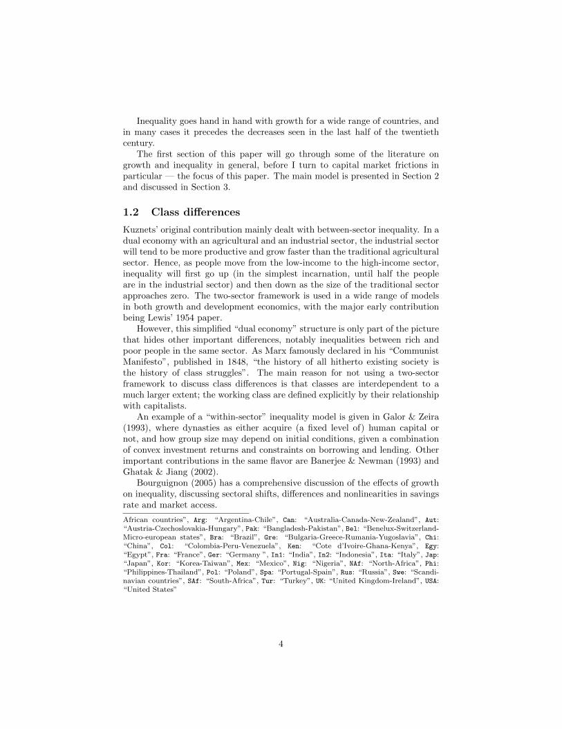
The inverse U-shape of inequality over time was pointed out by Kuznets (1955),and is illustrated in Figure 1 with data from Milanovic et al. (2007). Theupward-sloping part of this curve corresponds to the topic of this paper. Theearly Industrial Revolution saw a move from independent households to wagework. At the same time, capital markets as we know them today were notavailable for the larger part of the population. The theory behind this paper isthat this asymmetry in the institutional arrangement for the two major compo-nents of production — capital and labor — were strong drivers of the increasinginequality.

Documenting the increasing inequality in Europe during the early modernperiod is challenging because of the sparsity of data. However, most studiesargue that inequality was increasing, at least after 1500. Van Zanden (1995)argues that economic growth and inequality growth largely went together inEurope between 1500 and 1800. Hoffman et al. (2002) agree, and further dif-ferentiate the trend by looking at the price of various items in the consumptionbasket, identifying a general inequality-increasing trend in England, France andHolland between 1500 and 1650, as well as later inequality increases in all coun-tries.

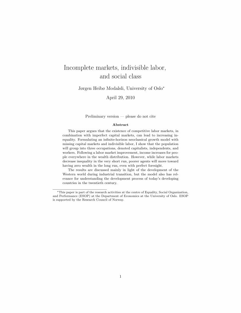
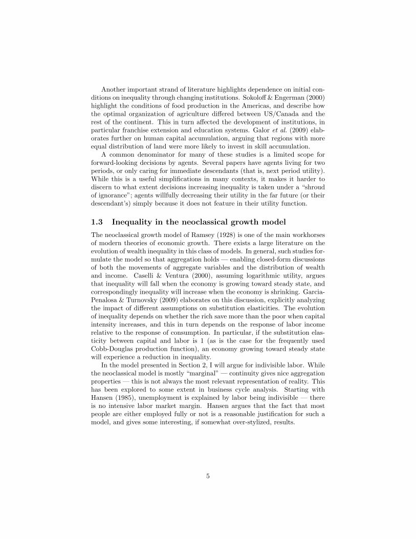
Moving to (comparatively) later periods, Figure 2 shows changes in theincome distribution in 33 different regions, as reported by Bourguignon & Mor-risson (2002).

The upper panel shows changes, where recorded, of the income share of thehighest 20%. It is evident that before 1910, all recorded changes are towardshigher shares for the rich, except for the United Kingdom and France. After1910 there are developments in both directions. The lower panel of Figure 2shows the income share of the poorest 20%. There is also here a clear trendtowards higher inequality; again only UK and France show a trend towards lessinequality in the early phase. 1

1Only points with recorded changes shown in the figure. Changes are in percentage points.Country key: Lat: “37 Latin American countries”, Asi: “45 Asian countries”, Afr: “46

2

30

40

50

60

70

Gin

i co

eff

icie

nt

(est

ima

ted

by

Mil

an

ov

ic e

t a

l (2

00

8))

UK

Netherlands

India

0

10

20

1200 1300 1400 1500 1600 1700 1800 1900 2000

Gin

i co

eff

icie

nt

(est

ima

ted

by

Mil

an

ov

ic e

t a

l (2

00

8))

Figure 1: The Kuznets curve — data from Milanovic et al. (2007)

AfrArg

Can

CanCan

Aut Aut

Aut

Aut

Bel Bel

Bel

Bel

Bra

Gre

Chi

Chi

Chi

Chi

ChiCol

KenKen

EgyFraFra

Fra Fra Fra Fra

Fra FraIn1 In1 In1

In2 In2 In2 In2In2

In2

Ita

Ita

Ita Ita

Jap

Jap

JapKor Kor

Kor

Mex

Mex

NigNig

NigNAfNAf

NAfNAf

Phi

Pol

Spa Spa

Spa Spa

Rus

Rus

Swe

Swe Swe

SweSAfSAf

SAfUK UK

UK

UK UK

UKUSAUSA

USA

USA

USA

USA

−.1

5−

.1−

.05

0.0

5C

hang

e in

sha

re o

f ric

hest

20%

1820−1850

1850−1870

1870−1890

1890−1910

1910−1929

1929−1950

1950−1960

1960−1970

1970−1980

1980−1992

Year

Afr Arg

CanCan

Aut AutAut

Aut

Bel Bel

Bel

Bel

Gre

ChiChi

Chi ChiKen

Ken

EgyFra Fra

Fra Fra Fra FraIn1 In1 In1

In2 In2In2 In2 In2

In2

Ita Ita Ita

Jap

Jap

JapKor

KorMex

MexNig Nig NigNAf

NAfPhi

Pol

Spa Spa

Rus

Swe

Swe SweSAfUK UK

UK UKUK

UKUSA USA

USA USAUSA

−.0

20

.02

.04

Cha

nge

in s

hare

of p

oore

st 2

0%

1820−1850

1850−1870

1870−1890

1890−1910

1910−1929

1929−1950

1950−1960

1960−1970

1970−1980

1980−1992

Year

Figure 2: Worldwide inequality — changes in income shares of rich and poor.Data from Bourguignon & Morrisson (2002)

3

Inequality goes hand in hand with growth for a wide range of countries, andin many cases it precedes the decreases seen in the last half of the twentiethcentury.

The first section of this paper will go through some of the literature ongrowth and inequality in general, before I turn to capital market frictions inparticular — the focus of this paper. The main model is presented in Section 2and discussed in Section 3.

1.2 Class differences

Kuznets’ original contribution mainly dealt with between-sector inequality. In adual economy with an agricultural and an industrial sector, the industrial sectorwill tend to be more productive and grow faster than the traditional agriculturalsector. Hence, as people move from the low-income to the high-income sector,inequality will first go up (in the simplest incarnation, until half the peopleare in the industrial sector) and then down as the size of the traditional sectorapproaches zero. The two-sector framework is used in a wide range of modelsin both growth and development economics, with the major early contributionbeing Lewis’ 1954 paper.

However, this simplified “dual economy” structure is only part of the picturethat hides other important differences, notably inequalities between rich andpoor people in the same sector. As Marx famously declared in his “CommunistManifesto”, published in 1848, “the history of all hitherto existing society isthe history of class struggles”. The main reason for not using a two-sectorframework to discuss class differences is that classes are interdependent to amuch larger extent; the working class are defined explicitly by their relationshipwith capitalists.

An example of a “within-sector” inequality model is given in Galor & Zeira(1993), where dynasties as either acquire (a fixed level of) human capital ornot, and how group size may depend on initial conditions, given a combinationof convex investment returns and constraints on borrowing and lending. Otherimportant contributions in the same flavor are Banerjee & Newman (1993) andGhatak & Jiang (2002).

Bourguignon (2005) has a comprehensive discussion of the effects of growthon inequality, discussing sectoral shifts, differences and nonlinearities in savingsrate and market access.

African countries”, Arg: “Argentina-Chile”, Can: “Australia-Canada-New-Zealand”, Aut:“Austria-Czechoslovakia-Hungary”, Pak: “Bangladesh-Pakistan”, Bel: “Benelux-Switzerland-Micro-european states”, Bra: “Brazil”, Gre: “Bulgaria-Greece-Rumania-Yugoslavia”, Chi:“China”, Col: “Colombia-Peru-Venezuela”, Ken: “Cote d’Ivoire-Ghana-Kenya”, Egy:“Egypt”, Fra: “France”, Ger: “Germany ”, In1: “India”, In2: “Indonesia”, Ita: “Italy”, Jap:“Japan”, Kor: “Korea-Taiwan”, Mex: “Mexico”, Nig: “Nigeria”, NAf: “North-Africa”, Phi:“Philippines-Thailand”, Pol: “Poland”, Spa: “Portugal-Spain”, Rus: “Russia”, Swe: “Scandi-navian countries”, SAf: “South-Africa”, Tur: “Turkey”, UK: “United Kingdom-Ireland”, USA:“United States”

4

Another important strand of literature highlights dependence on initial con-ditions on inequality through changing institutions. Sokoloff & Engerman (2000)highlight the conditions of food production in the Americas, and describe howthe optimal organization of agriculture differed between US/Canada and therest of the continent. This in turn affected the development of institutions, inparticular franchise extension and education systems. Galor et al. (2009) elab-orates further on human capital accumulation, arguing that regions with moreequal distribution of land were more likely to invest in skill accumulation.

A common denominator for many of these studies is a limited scope forforward-looking decisions by agents. Several papers have agents living for twoperiods, or only caring for immediate descendants (that is, next period utility).While this is a useful simplifications in many contexts, it makes it harder todiscern to what extent decisions increasing inequality is taken under a “shroudof ignorance”; agents willfully decreasing their utility in the far future (or theirdescendant’s) simply because it does not feature in their utility function.

1.3 Inequality in the neoclassical growth model

The neoclassical growth model of Ramsey (1928) is one of the main workhorsesof modern theories of economic growth. There exists a large literature on theevolution of wealth inequality in this class of models. In general, such studies for-mulate the model so that aggregation holds — enabling closed-form discussionsof both the movements of aggregate variables and the distribution of wealthand income. Caselli & Ventura (2000), assuming logarithmic utility, arguesthat inequality will fall when the economy is growing toward steady state, andcorrespondingly inequality will increase when the economy is shrinking. Garcia-Penalosa & Turnovsky (2009) elaborates on this discussion, explicitly analyzingthe impact of different assumptions on substitution elasticities. The evolutionof inequality depends on whether the rich save more than the poor when capitalintensity increases, and this in turn depends on the response of labor incomerelative to the response of consumption. In particular, if the substitution elas-ticity between capital and labor is 1 (as is the case for the frequently usedCobb-Douglas production function), an economy growing toward steady statewill experience a reduction in inequality.

In the model presented in Section 2, I will argue for indivisible labor. Whilethe neoclassical model is mostly “marginal” — continuity gives nice aggregationproperties — this is not always the most relevant representation of reality. Thishas been explored to some extent in business cycle analysis. Starting withHansen (1985), unemployment is explained by labor being indivisible — thereis no intensive labor market margin. Hansen argues that the fact that mostpeople are either employed fully or not is a reasonable justification for such amodel, and gives some interesting, if somewhat over-stylized, results.

5

1.4 Capital market imperfections

The question of saving is at the core of neoclassical growth theory (Ramsey’s1928 paper is titled “A Mathematical Theory of Saving”) and usually one of twoassumptions is taken on capital markets: they are internationally open, whichgives a convenient constant interest rate, or internationally closed, but nationallyopen, which usually gives a unique domestic interest rate. For the purpose ofsolving a model which heterogeneous agents, a lot of whom are very poor, Iwill argue that another assumption is more natural: that capital markets arenot accessible. True, for the rich, advanced instruments for facilitating capitalusage have existed for at least half a millennium. But for the poor, this is notthe case.2

I have not found much evidence of how poor farmers and workers saved inprevious centuries. There does, however, exist a growing literature on miss-ing financial markets in today’s developing countries, and there is no reason tobelieve that conditions in, for example, fourteenth-century England were anybetter than in twentieth-century Bangladesh. Rutherford & Arora (2009) ar-gues that there is a huge, unmet demand for saving services by poor people indeveloping countries. They give examples of savings products where adminis-trative fees would correspond to an annualized interest rate of minus 30% (withthe depositor still bearing all risk for “bank failure” of the informal deposit col-lector) — which are envied by residents of neighboring areas who have no accessto semiformal saving at all. Similar stories — of how financial instruments haveto be improvized for 40% of the people alive today — is given in Collins et al.(2009).

The contribution of capital market frictions to firm and growth dynamicsis being steadily more explored in the literature. Song et al. (2009) argue thatraising capital internally — financing investment out of savings — is an impor-tant feature of the private sector in China, and that differences in capital accessexplain why low-productivity state-run firms coexist with high-productivity pri-vate firms.

1.5 A capital market theory of economic development

Though the model presented in this paper can be used to analyze any economywith insufficient credit market institutions, it is conceived to fit into the upward-sloping part of the Kuznets curve, as a transition state between a subsistenceeconomy (Phase I in the list below) and a modern market economy (PhaseIII). The polarizing results of the model are best understood within such aframework:

• Phase I: Capital ownership is fixed (for example as farms; no institu-tion for purchase and sale of land titles). If there is no labor market

2In the model to be presented in Section 2, the “no credit market” assumption is notbinding for the rich; it would not change the outcome of the model if the credit marketassumptions were restricted to the poor. For clarity, I therefore postulate a model with nocredit markets altogether.

6

(because of big distances between farms, missing institutions, serfdom, orland abundance) production and income is fixed. The fixed distribution ofthis phase (depending on geographical, social and economic mechanismsoutside the model) gives the initial conditions for the transition discussedin this paper.

• Phase II: Labor can be freely “rented” (that is, employed). Capital can bebought and sold but no rental. This can be thought of as the early frame-work of the Industrial Revolution, or as today’s reality for poor people indeveloping countries. This is the “transition to inequality” presented inthis paper; the upward-sloping part of the Kuznets curve.

• Phase III: Capital rental allowed. This gives credit market access for all,and a modern society with inequality, but without marked class differ-ences. This is the “neoclassical model” that is well discussed in the liter-ature as mentioned in Section 1.3 (Garcia-Penalosa & Turnovsky (2009)and others). This is the downward-sloping part of the Kuznets curve,where some of the inequalities of Phase II will be reversed. I will returnto this in the final section of the paper.

This evolution of institutions is not meant to explain all aspects of inequalitydevelopment over time. There is clearly merit to Kuznets’ story of the dual econ-omy, and other mechanisms at work as well. The contribution of this discussionis the emergence of inequality in interdependent relationships; both workers andcapitalists becoming more defined as groups precisely by interacting with eachother.

2 Model

The main feature distinguishing this model from most other heterogeneous-agent models is an assumption that capital can only be successfully used by itsowner. In a society of limited trust and institutional enforcement, how can thelender know that the borrower will use the capital in a sustainable way? I takethe representation of the moral hazard problem “all the way” in the sense thatI do not allow for rental of capital at all. In addition, I assume that the capitalowners cannot split their own time between working with their own capital andbeing regular wage workers in someone else’s firm. 3 These assumptions canalternatively be rationalized from a geographic point of view: given location-bound capital (land, farm buildings, resource claims) capital may not be easilytransportable, and the labor markets (in cities or at larger farms) may not besituated in the same place as the agent’s own capital. As will be shown, theresult of these restrictions is the emergence of three distinct occupations, which Iwill identify with social class: Workers, for whom it’s more profitable to work atsomeone else’s firm than using their own capital; capitalists, who own enough

3If they could, it can be shown that the previous restriction would not lead to a departurefrom the capital-rental model.

7

capital to make hiring workers profitable, and independents, who work usingtheir own capital but do not hire other workers. 4 While the first two groups areeasily identifiable with nineteenth-century stereotypes, the independent groupis not as easy to conceptualize; later, I will discuss interpretations of this groupas subsistence farmers and as independent “professionals”.

As there are no credit markets in the model, the “capital” discussed can justas easily be human capital as physical capital, provided that mass-market jobsdo not permit use of this human capital. For simplicity, the language below willrefer to physical capital.

The choice of modeling utility with an infinite horizon makes the model morecomplex. This decision is partly motivated by the fact that one of the charac-teristics of the working class is low return to capital. Even within one’s ownlifetime, saving enough to escape this position may not be possible. However,there is a possibility of passing on to future generations a slightly improvedposition in society, leading to potential upward mobility. To incorporate suchmechanisms, the unit of decision-making in the model presented here will be thedynasty; with the presently active agent caring for all future generations, deci-sions that sacrifice some consumption today for potential future improvementswill be important.

2.1 Production, consumption and saving

Agents are infinitely lived dynasties that maximize expected discounted utilityof consumption.

max{ci,τ}∞τ=t

Et

∞∑τ=t

βτ−tu(ci,τ ) (1)

The function u(c) is concave and satisfies the Inada conditions. In the equi-

librium solutions below, I will use the CRRA function form u(ct) = (ct)1−η

1−ηProduction takes place in a continuum of constant-returns-to-scale firms with

the Cobb-Douglas production function

yi,t = (ki,t)α(Ztli,t)

1−α (2)

where Zt is level of technological progress, growing at a constant rate. Inthe following exposition, Z will be assumed constant. It is shown in Section 2.3that the result carries over to the case of constant technological growth.

The budget constraint for the individual is

ci,t + ai,t+1 = m(ai,t, si,t, wt) (3)

4A similar three-occupation result is found in Banerjee & Newman (1993).

8

The function m defines the agent’s income as a function of wealth a, occu-pation s (worker or entrepreneur, to be defined below), a variable representingindividual uncertainty ε and the going wage level w.

As discussed above, there are two possible “labor market outcomes”:A wage worker gets the going market wage w times his labor productivity

level. For this exercise, I will assume constant labor productivities, normalizedto 1. In addition to labor income, the wage worker’s capital can be stored, witha return ν ≤ 1. The income function hence is

m(ai,t,worker, wt) = wt + νai,t (4)

An entrepreneur does not work for hire and uses his wealth for production,and is hence denoted as the owner of a firm.

There is only one type of capital, hence ki,t = ai,t when production is chosen.The entrepreneur’s maximization problem is to hire the amount of labor ι thatmaximizes output minus wage costs:

maxιi,t

aαi,tZ1−αt (1 + ι)1−α − wι (5)

From this, optimal labor demand can be shown to be

ι∗i,t = w− 1α

t (1− α)1αZ− 1−α

αt ai,t − 1 (6)

and a corresponding income (profit) function can be derived. However, asentrepreneurs cannot be workers at the same time, ι cannot be negative. If

If ι∗ < 0, that is w− 1α

t (1 − α)1αZ

1−αα

t ai − 1 < 0, meaning wealth is below thethreshold

ac(wt, Zt) = w1αt (1− α)−

1αZ− 1−α

αt (7)

no labor is hired, and income is just the production function with the agent’sown labor inserted. This constrained type of agent (with a < ac) is hence notparticipating in the labor market, and is identified with the “independent” agentdiscussed above.

When capital is used productively, it depreciates uniformly at a rate δ.To sum up, the income of the entrepreneur is given by

m(ai,t, entrepreneur, wt) = (1− α)1−αα αZ

1−αα

t w− 1−α

αt ai,t + w + (1− δ)ai,tif ai,t ≥ ac(wt, Zt) (“independent”)

(8)

m(ai,t, entrepreneur, wt) = aαi,tZ1−αt + (1− δ)ai,t if a < ac(wt, Zt) (“capitalist”)

(9)

9

The lower bound on a is set to 0 (no borrowing allowed), to be consistentwith the assumptions on capital rental.

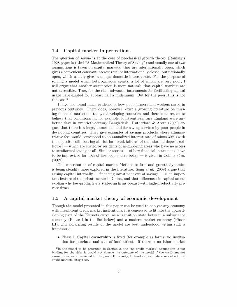
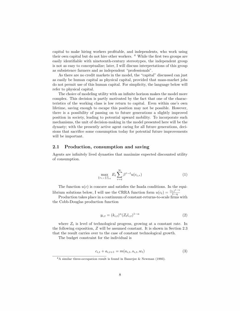
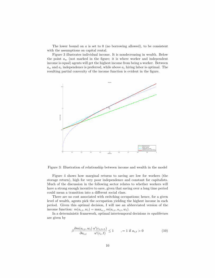
Figure 3 illustrates individual income. It is nondecreasing in wealth. Belowthe point aw (not marked in the figure; it is where worker and independentincome is equal) agents will get the highest income from being a worker. Betweenaw and ac independence is preferred, while above ac hiring labor is optimal. Theresulting partial convexity of the income function is evident in the figure.

0 0.1 0.2 0.3 0.4 0.5 0.6 0.7 0.8 0.9 10

0.5

1

1.5

Assets a

Inco

me

m(a

)

Income

¬ ac

Realized incomeWorker incomeIndependent incomeCapitalist income (only if a>a

c)

Figure 3: Illustration of relationship between income and wealth in the model

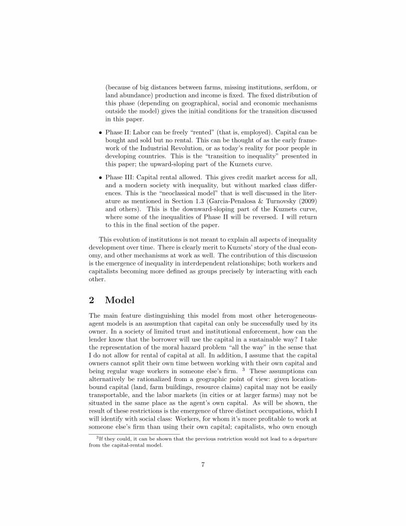
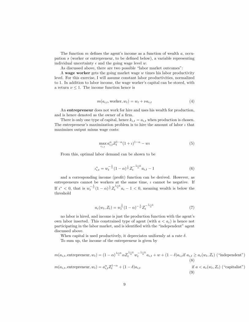
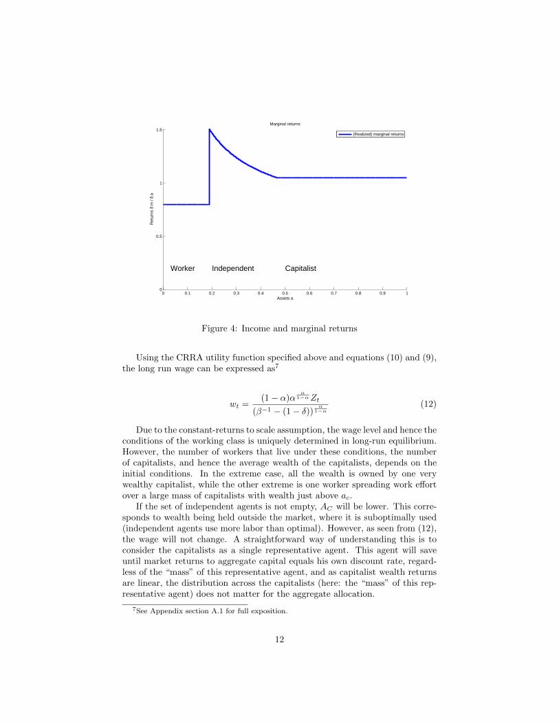
Figure 4 shows how marginal returns to saving are low for workers (thestorage return), high for very poor independence and constant for capitalists.Much of the discussion in the following sector relates to whether workers willhave a strong enough incentive to save, given that saving over a long time periodcould mean a transition into a different social class.

There are no cost associated with switching occupations; hence, for a givenlevel of wealth, agents pick the occupation yielding the highest income in eachperiod. Given this optimal decision, I will use an abbreviated version of theincome function: m(ai,t, wt) = maxsi,t m(ai,t, si,t, wt).

In a deterministic framework, optimal intertemporal decisions in equilibriumare given by

β∂m(ai,t, wt)

∂ai,t

u′(ci,t+1)

u′(ci, t)≤ 1 ,= 1 if ai,t > 0 (10)

10

However, outside equilibrium, agents’ wealth might not be stationary. As∂m∂a is not continuous, this leads to problems with derivative methods, and op-timization is better characterized by value function methods, as illustrated in alater section.

2.2 Wage determination and labor market clearing

Following the discussion above, there are three groups of agents (“occupations”)in the economy. I will denote the workers, independents and capitalists asbelonging to the sets LW , LI and LC respectively. The mass of agents in eachgroup is denoted Lj , with LW + LI + LC = 1 — no population growth. I willdenote the total wealth holdings of each group as Aj =

∑i∈Lj ai.

As there is no rental market for capital, the interest rate r will not beobserved in the market.5 There are two markets that clear each period: themarket for the final good (divided between consumption and investment), andthe market for labor. As is conventional, the price of the consumption andinvestment good is normalized to 1. The wage rate is determined in the labormarket.

The supply of labor is given by∑LW 1 = LW . The demand for labor is

given by∑i∈LC ι

∗i . Setting supply equal to demand yields the market clearing

wage

wt = (1− α)Z1−αt

(AC,t

LC,t + LW,t

)α(11)

Note that the mass and wealth holdings of the independent group does notfeature in the wage equation. The workers’ stored capital, not part of produc-tion, also does not influence the market wage.

2.3 Steady state

Assuming that at least some capitalists and workers exist in the long-run equilib-rium,6 it follows from concavity of utility (Equation 1) and linearity of capitalistreturns (Equation 9, see also Figure 4) that at some point the marginal utility ofsaving will equal the marginal utility from consumption. As shown by Chatter-jee (1994), the within-group distribution of wealth is not required to calculatethe aggregate behavior of this group. Because the labor market smooths sav-ing for this group, they act as if there was full capital market access, and thecorresponding theoretical price of capital — the return rate in Equation (9) —will have a determined value in the long run. Hence, the long-run equilibriumwage can also be easily calculated.

5However, for the capitalist agents return to capital is still linear, so even without tradereturns will be uniform for rich agents.

6This has not been shown in detail. Theoretically there can be only independents in thelong run, but this requires a very compressed wealth distribution and would likely be unstableto small perturbations

11

0 0.1 0.2 0.3 0.4 0.5 0.6 0.7 0.8 0.9 10

0.5

1

1.5

Assets a

Ret

urns

δ m

/ δ

a

Marginal returns

Worker Independent Capitalist

(Realized) marginal returns

Figure 4: Income and marginal returns

Using the CRRA utility function specified above and equations (10) and (9),the long run wage can be expressed as7

wt =(1− α)α

α1−αZt

(β−1 − (1− δ))α

1−α(12)

Due to the constant-returns to scale assumption, the wage level and hence theconditions of the working class is uniquely determined in long-run equilibrium.However, the number of workers that live under these conditions, the numberof capitalists, and hence the average wealth of the capitalists, depends on theinitial conditions. In the extreme case, all the wealth is owned by one verywealthy capitalist, while the other extreme is one worker spreading work effortover a large mass of capitalists with wealth just above ac.

If the set of independent agents is not empty, AC will be lower. This corre-sponds to wealth being held outside the market, where it is suboptimally used(independent agents use more labor than optimal). However, as seen from (12),the wage will not change. A straightforward way of understanding this is toconsider the capitalists as a single representative agent. This agent will saveuntil market returns to aggregate capital equals his own discount rate, regard-less of the “mass” of this representative agent, and as capitalist wealth returnsare linear, the distribution across the capitalists (here: the “mass” of this rep-resentative agent) does not matter for the aggregate allocation.

7See Appendix section A.1 for full exposition.

12

To this point, the model has been discussed as if the technology level Z wasconstant. It is straightforward to show that with appropriate variable substitu-tion, the results hold for constant exogenous technological growth; see Appendix(A.1).

Denoting the growth rate of Z as g, the relevant substitutions are to multiplythe initial technological level Z0 as well as the variables a and w with exp(gt)in all time periods.

The discount rate β in Equation (1) is replaced with β = β exp(g(1 − η)).For η > 1, this sets an lower bound to technological growth for any value of β— if β is higher than 1, agents would want to move consumption forward intime beyond consumption smoothing motivations, and some of the results inthe model would not hold. In the following, constant technological level Z willbe assumed in the exposition, and the relevant substitutions will be made whencalibration is discussed.

While the steady-state can serve as a discussion platform for some inequal-ity issues, my main interest in this paper is the transition to this steady state.Primarily, the model has a multi-generation interpretation that allows for thetransition to take a long time (up to several hundred years). As the institutionalsetup does not correspond to that observed today in rich countries, it is reason-able to believe that at some point capital markets will be improved, increasingsavings opportunities for the poor. To solve for this transition, I have to relyon numerical methods. This will be the scope of the next section.

3 Economic transition

The transition to steady state is a period of increasing inequality and an emer-gence of new social classes. Poorer people become poorer over time, while thosewith higher wealth consolidate into a capitalist group.

The dynamics of the transition can be characterized as three-stage process:Initial adjustment. As the labor market opens, individuals immediately

adjust, with the poorest becoming workers instead of independent producers.This happens before capital can be adjusted.

Workers’ wealth adjustment. Over time, those who are going to end upas workers in the long run will run down their wealth.

Capitalists’ wealth adjustment. Over time (usually a longer time framethan for the workers, as discussed below), overall capitalist wealth adjusts to thesteady-state level. The distribution among capitalists in steady state dependson the initial distribution.

As mentioned above, because the income function is not smooth, solvingfor the transition cannot rely on taking derivatives; I will therefore solve foroptimal decisions using the value function directly. Because switching betweenoccupations from period to period is frictionless, the wealth level a fully sumsup any individual’s possibilities. For a given wage path w, the value functionV (a,w) denotes present utility of all future consumption. At any time, theindividual faces the choice

13

maxat+1

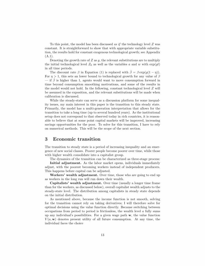
u(m(at, wt)− at+1) + βV (at+1,w) (13)

Proposition 1 Agents’ paths of wealth over time will not cross.

Proof: See appendix (A.1).[add section on potential “all-autarky” solution here; requires some simple

calculations on initial conditions]

3.1 Calibration

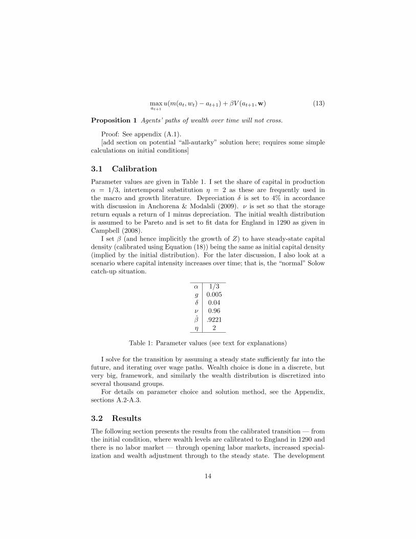
Parameter values are given in Table 1. I set the share of capital in productionα = 1/3, intertemporal substitution η = 2 as these are frequently used inthe macro and growth literature. Depreciation δ is set to 4% in accordancewith discussion in Anchorena & Modalsli (2009). ν is set so that the storagereturn equals a return of 1 minus depreciation. The initial wealth distributionis assumed to be Pareto and is set to fit data for England in 1290 as given inCampbell (2008).

I set β (and hence implicitly the growth of Z) to have steady-state capitaldensity (calibrated using Equation (18)) being the same as initial capital density(implied by the initial distribution). For the later discussion, I also look at ascenario where capital intensity increases over time; that is, the “normal” Solowcatch-up situation.

α 1/3g 0.005δ 0.04ν 0.96

β .9221η 2

Table 1: Parameter values (see text for explanations)

I solve for the transition by assuming a steady state sufficiently far into thefuture, and iterating over wage paths. Wealth choice is done in a discrete, butvery big, framework, and similarly the wealth distribution is discretized intoseveral thousand groups.

For details on parameter choice and solution method, see the Appendix,sections A.2-A.3.

3.2 Results

The following section presents the results from the calibrated transition — fromthe initial condition, where wealth levels are calibrated to England in 1290 andthere is no labor market — through opening labor markets, increased special-ization and wealth adjustment through to the steady state. The development

14

is described in Section 1.5, where I hypothesize that either before or after thesteady state in this model is reached, modern capital markets start to improve,leading to savings opportunities for the poor in the long run, outside this model.

3.2.1 Occupational choice

0 10 20 30 40 50 600

0.1

0.2

0.3

0.4

0.5

0.6

0.7

0.8

0.9

1

WorkerIndependentCapitalist

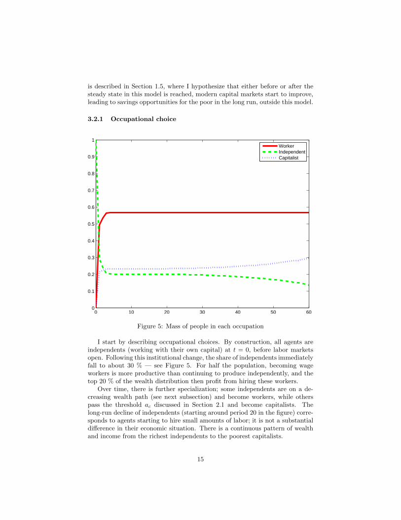
Figure 5: Mass of people in each occupation

I start by describing occupational choices. By construction, all agents areindependents (working with their own capital) at t = 0, before labor marketsopen. Following this institutional change, the share of independents immediatelyfall to about 30 % — see Figure 5. For half the population, becoming wageworkers is more productive than continuing to produce independently, and thetop 20 % of the wealth distribution then profit from hiring these workers.

Over time, there is further specialization; some independents are on a de-creasing wealth path (see next subsection) and become workers, while otherspass the threshold ac discussed in Section 2.1 and become capitalists. Thelong-run decline of independents (starting around period 20 in the figure) corre-sponds to agents starting to hire small amounts of labor; it is not a substantialdifference in their economic situation. There is a continuous pattern of wealthand income from the richest independents to the poorest capitalists.

15

The figure as shown is for constant capital density; I will return to the caseof increasing capital density below (Section 3.2.5).

3.2.2 Wealth accumulation

0 50 100 1500

0.5

1CDF, wealth. t=1

0 50 100 1500

0.5

1CDF, wealth. t=2

0 50 100 1500

0.5

1CDF, wealth. t=3

0 50 100 1500

0.5

1CDF, wealth. t=4

0 50 100 1500

0.5

1CDF, wealth. t=6

0 50 100 1500

0.5

1CDF, wealth. t=10

0 50 100 1500

0.5

1CDF, wealth. t=20

0 50 100 1500

0.5

1CDF, wealth. t=30

0 50 100 1500

0.5

1CDF, wealth. t=60

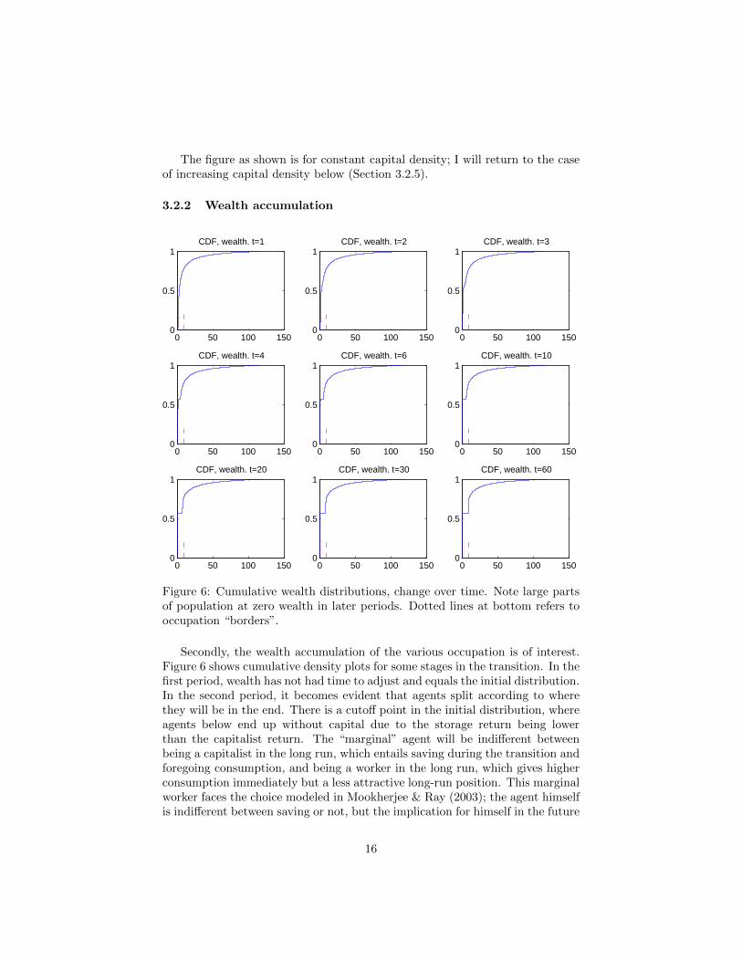
Figure 6: Cumulative wealth distributions, change over time. Note large partsof population at zero wealth in later periods. Dotted lines at bottom refers tooccupation “borders”.

Secondly, the wealth accumulation of the various occupation is of interest.Figure 6 shows cumulative density plots for some stages in the transition. In thefirst period, wealth has not had time to adjust and equals the initial distribution.In the second period, it becomes evident that agents split according to wherethey will be in the end. There is a cutoff point in the initial distribution, whereagents below end up without capital due to the storage return being lowerthan the capitalist return. The “marginal” agent will be indifferent betweenbeing a capitalist in the long run, which entails saving during the transition andforegoing consumption, and being a worker in the long run, which gives higherconsumption immediately but a less attractive long-run position. This marginalworker faces the choice modeled in Mookherjee & Ray (2003); the agent himselfis indifferent between saving or not, but the implication for himself in the future

16

(or his descendants) are different depending on the choice taken. Those belowthe choice threshold start to run down their wealth, even if they are still wealthyenough not to choose wage labor in the short run; in the long run, they will alsobecome wage workers. This group explains the increase in the worker occupationin period 1-4 as shown in Figure 5. Over time, the wealth of workers approachzero.

0 10 20 30 40 50 600

1

2

3

4

5

6

7

8

Capital held by workersCapital held by independentsCapital held by capitalists

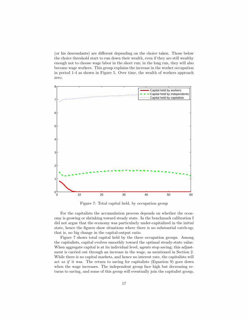
Figure 7: Total capital held, by occupation group

For the capitalists the accumulation process depends on whether the econ-omy is growing or shrinking toward steady state. In the benchmark calibration Idid not argue that the economy was particularly under-capitalized in the initialstate, hence the figures show situations where there is no substantial catch-up;that is, no big change in the capital-output ratio.

Figure 7 shows total capital held by the three occupation groups. Amongthe capitalists, capital evolves smoothly toward the optimal steady-state value.When aggregate capital is at its individual level, agents stop saving; this adjust-ment is carried out through an increase in the wage, as mentioned in Section 2.While there is no capital markets, and hence no interest rate, the capitalists willact as if it was. The return to saving for capitalists (Equation 9) goes downwhen the wage increases. The independent group face high but decreasing re-turns to saving, and some of this group will eventually join the capitalist group,

17

as shown in Figure 5, while others will stay just below the limit. As statedabove, and seen in Figure 6, the move from independent to capitalist does notentail a jump in wealth.

3.2.3 Within-group inequality

0 20 40 600

0.5

1

1.5

2

2.5

3Workers

0 20 40 602

4

6

8

10Independents

0 20 40 600

20

40

60

80

100

120Capitalists

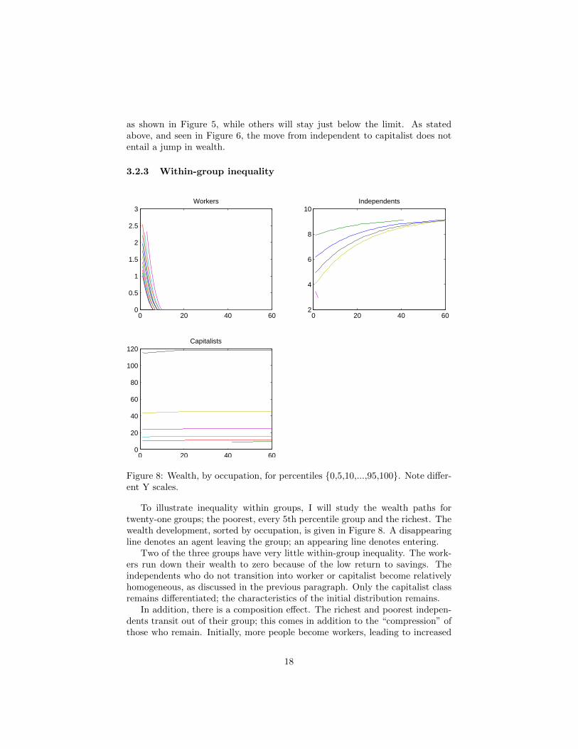
Figure 8: Wealth, by occupation, for percentiles {0,5,10,...,95,100}. Note differ-ent Y scales.

To illustrate inequality within groups, I will study the wealth paths fortwenty-one groups; the poorest, every 5th percentile group and the richest. Thewealth development, sorted by occupation, is given in Figure 8. A disappearingline denotes an agent leaving the group; an appearing line denotes entering.

Two of the three groups have very little within-group inequality. The work-ers run down their wealth to zero because of the low return to savings. Theindependents who do not transition into worker or capitalist become relativelyhomogeneous, as discussed in the previous paragraph. Only the capitalist classremains differentiated; the characteristics of the initial distribution remains.

In addition, there is a composition effect. The richest and poorest indepen-dents transit out of their group; this comes in addition to the “compression” ofthose who remain. Initially, more people become workers, leading to increased

18

wealth dispersion in this group as people enter, but dispersion goes down overtime as wealth stabilizes at zero and no more entries occur. Similarly, for capi-talists, there is an inflow of people at the bottom, but here this effect is dwarfedsomewhat by the overall dispersion of wealth.

3.2.4 Wage path

0 10 20 30 40 50 601.37

1.38

1.39

1.4

1.41

1.42

1.43

wage

Figure 9: Wage

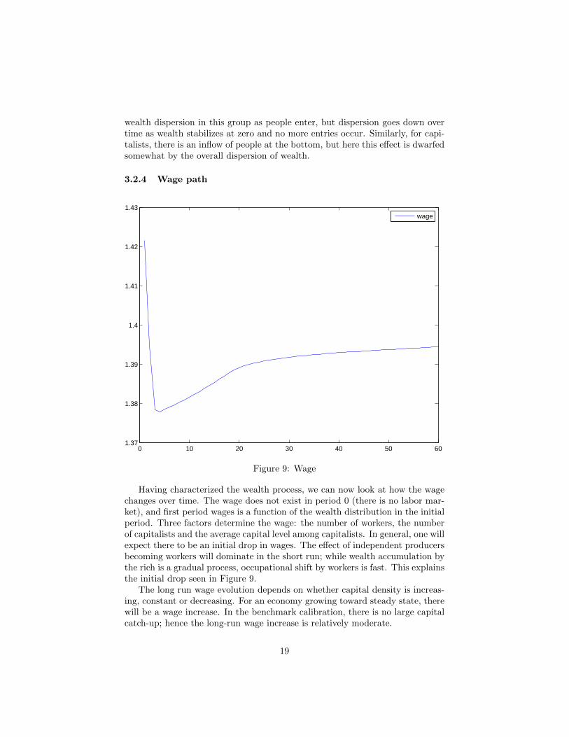
Having characterized the wealth process, we can now look at how the wagechanges over time. The wage does not exist in period 0 (there is no labor mar-ket), and first period wages is a function of the wealth distribution in the initialperiod. Three factors determine the wage: the number of workers, the numberof capitalists and the average capital level among capitalists. In general, one willexpect there to be an initial drop in wages. The effect of independent producersbecoming workers will dominate in the short run; while wealth accumulation bythe rich is a gradual process, occupational shift by workers is fast. This explainsthe initial drop seen in Figure 9.

The long run wage evolution depends on whether capital density is increas-ing, constant or decreasing. For an economy growing toward steady state, therewill be a wage increase. In the benchmark calibration, there is no large capitalcatch-up; hence the long-run wage increase is relatively moderate.

19

3.2.5 The effects of changing capital density

The above discussion is for a result where capital density is not increasing towardequilibrium. This would mean that all growth in the period covered by themodel was technological, and that aggregate capital accumulation did not playan important role.

If one alternatively argue that capital accumulation was important, thatis that the economy is under-capitalized in period 0, the long-run paths looksomewhat different.

The long-run wage development will be increasing; the short-run drop willgenerally be seen, but can be dwarfed by later increases. This is similar toa model without frictions, where increased capital density drives up wages.The effect on occupational choice is ambiguous; while wages are higher, so arecapitalist returns, and as higher long-run capital density implies more forward-looking agents, higher weight will be attached to the future and less to thepresent, making the “capitalist” role more attractive for given wealth.

All wages and wealth sizes in the figures are given for constant technology; asdiscussed in Section 2.3, individual wealth and wage grows at the same rate asthe exogenous technology growth, both during the transition and in equilibrium.The growth-adjusted values are found by multiplying the shown values withZ0 exp(gt).

3.3 Discussion

In this section I will present a more general discussion of the mechanisms atwork in the model. I will also draw some comparisons to modern developingcountries, and discuss the relevance of the model.

3.3.1 Polarization

Even though wages increase during the transition to steady state, inequalityis increasing. Because the capitalists are also supplying labor effort, wage in-creases (which are results of capital accumulation) cannot help in closing the gapbetween rich and poor.8 Even with the human capital interpretation of modelwealth, where a is interpreted more broadly as both human and non-humancapital, there is a component of “raw” labor (l) of which the rich get the samereward for any wage increase as the poor do.

There is no explicit “subsistence income” in the model. However, if theequilibrium wage is at a very low level — corresponding to a low equilibriumcapital density — one could imagine that employers would get productivity gainsby increasing wages, for example through workers eating better. This higherwage would then correspond to a “job lottery” and unemployment would arise.This is similar to the mechanisms in Harris & Todaro (1970), and would herebe explained through low savings propensities. These could again be caused by

8The only way to have wage increases lowering inequality would be to have several typesof labor with imperfect substitutability (such as high- and low-skill labor).

20

high systemic uncertainty — risk of expropriation, war or disease — increasingprobability of a future state where current saving don’t matter effectively workslike a lower discount rate, and hence a reduced focus on the future.

If, in modern society, there are some jobs that do not require human capitalat all, we can imagine an inequality-inducing process like the one portrayedin this paper. Those using human capital in their daily work have a higherincentive to accumulate more. Those who do not have daily use of humancapital choose not to accumulate — not because they have different preferences,but simply because they do not earn the same return to it. In this example the“initial wealth” would be human capital “inherited” by parents. If this line ofthought holds, it means that low-paid low-skill jobs are not likely to disappearwith economic growth; while markets for physical capital and monetary wealthare now relatively well-developed in many parts of the world, markets for humancapital (where a person holds his low-skill job while renting his human capitalto a person in a high-skill job) do not seem likely to appear.

3.3.2 Rational poverty

A key element of the model results is “rational poverty” — by the standarddefinitions, it is optimal for the agents in the lower end of the wealth spectrumto run down their wealth and become workers in the long run, even if saving andbecoming a capitalist is feasible by reducing current consumption. Of course,in real world applications, many other factors are responsible for poverty, andthis paper does not address any of those. If uncertainty was introduced to themodel, for example through stochastic labor productivity or wealth returns,some mobility could ensue, and there would be savings also among poor people;such precautionary savings are reported for example by Collins et al. (2009) andwill be discussed in a later paper.9

However, the model does capture an important point: if returns for poorpeople are lower, they will save less. Is this a “poverty trap”? On the individuallevel, perhaps; if one person was initially given a large transfer, he would haveended up a capitalist instead. But the existence of the working class can not bedone away with. In this model, for any equilibrium, there will be some peoplefor whom it is profitable to work, and these people will have zero wealth in thelong run.

3.3.3 Who are the independents?

In the model, “workers” work full-time for wages and have no capital income,and “capitalists” own firms and get the residual income from them. It shouldnot be difficult for the reader to conjure images of members of these groups, beit in eighteenth century England or twentieth century Uganda. But who are the“independents”?

I have been intentionally vague on the interpretation of the “capital” measurein this model. Starting with a predominantly agricultural economy, land and

9There is presently some discussion on this in the Appendix, section A.4.1.

21

farms are the most important elements in production. Independents wouldhence be self-sufficient farmers; a group with great heterogeneity. Improvinglabor markets would then “eat away” at the bottom of this distribution, aspoor farmers seek employment on big farms or in cities. They would also “eataway” at the top, as large farms could expand their production by hiring labor.Hence, the decline in subsistence agriculture is consistent with the model.

The notion of “independent” in this model also has a counterpart in moderndeveloped countries. While markets for physical capital are fairly well developed(the recent financial crisis notwithstanding), there are still no markets for rentinghuman capital. Hence, many professional workers — doctors, lawyers, artists,others — organize their work independently, through self-employment or smallpartnerships. They can be contrasted from those holding large wealth, andhence owning big companies, and those who work in these big companies.

3.3.4 The scope for equalizing policies

A one-time lump-sum transfer to a worker can be so big as to lift the workerout of his class. This does, however, for the current calibration correspondto several times the per-period wage. [note: calculate this exactly]. Smallertransfers will improve welfare in the short run and have no effect in the longrun. It follows that in order to work, poverty alleviating policies needs to be inforce continuously, for example in the form of tax-and-transfer schemes.

[Feasibility of tax-and-transfer schemes here]As an alternative to tax-and-transfer schemes, one could consider other poli-

cies such as regulating the wage level. Assuming that this could be done andenforced properly, which is not a trivial matter, this would largely work in thesame way as taxes; wage costs would go up, leading to reduced capital accumu-lation.

3.4 The effects of different initial conditions

Overall capital density in steady state follows directly from the model parame-ters. This illustrates that high-wealth agents can “crowd out” moderate-wealthagents from the steady-state wealth distribution. If, initially, some agents havehigh capital levels, more of the capital will be used in firms participating in thelabor market, bidding up wages. This will lead to some intermediate agentschoosing the “wage path” instead of the “capitalist path”, giving a higher frac-tion of workers in the long run.

There should be some scope for dependence on the initial distribution. Buthow much? If capital density is initially high, wages should be higher in thetransition period, decreasing the utility of being a capitalist. The marginal agentshould hence be expected to be richer if capital density is higher, as returns tosaving are lower. In a sense, the existence of more rich agents “crowd out” thesavings incentives of intermediate agents.

However, marginal agents tend to be independents for quite a large periodof the transition. When independent, the wage does not affect their income,

22

only their eventual transition out of the group. This should work to make theeffect smaller.

To see if the effect is quantitatively big, I rescaled the initial distribution usedin Section 3.2 to be 98 % of its original size. The remaining 2 % got a wealthhigher than the previous maximum. Then, I compare two different values forthis higher group. This means that the main part of the distribution is fixed,only at the top is there a small change. I denote as the “low” scenario thecase where the wealthiest 2 % have a wealth of 130, and as the “high” scenariowhere the wealth is 160. I do this for both the “constant capital density” and“increasing capital density” cases.

It turns out that the resulting wealth and occupation distribution is notmuch affected by this change. Wages are always lower in the “low” scenario,but only by fractions of a percentage point. Similarly, the resulting occupationdistributions do not differ much: for example, in the “constant capital” scenario,the share of workers in steady state only increases from 63.3% to 63.7%.

[also: Varying mean and SD of initial distribution. To be written]

4 Summing up

Though the main focus in this paper has been on historical inequality, themechanisms also have relevance in today’s developing countries. The main pol-icy implication is that capital market access for the poor should be improved;indeed there has been a major push in this direction in development policiesover the last decades (see for example Collins et al. (2009)).

The model has accounted for one reason while inequality can have increasedover the centuries leading up to and including the Industrial Revolution. In-divisibilities in labor, combined with a missing capital markets, lead to a largegroup of the population not holding wealth in the long run, instead choosingwage work for themselves and their descendants. While the standard mecha-nisms of the neoclassical growth model operates for the richer part of the wealthdistribution, it does not apply to the poor.

The model predicts a relatively sharp transition into a homogeneous workingclass. While the emergence of industrial cities in Great Britain in the eighteenthcentury was fast, the model probably does overstate this effect to some extent;after all, agricultural labor markets were in existence before the Industrial Rev-olution. In addition, power politics has always played a role in the allocation ofproductive factors, and when looking at any given country over a time periodof this length, wars, revolutions and other “shocks”, as well as technologicaldevelopments, are likely to interact with any economic process. However, theoverall picture — that of increasing occupational polarization — seems a goodfit, and I will argue that this model, combined with the “capital market theoryof economic development” discussed in Section 1.5, is a substantial contributiontoward understanding this process.

Apart from capital market improvements there does not seem to be muchscope for permanent improvements to the conditions of the working class in

23

this model. Removing the indivisibility of labor would allow small-scale en-trepreneurship beside wage work. However, most places in the world, workseems to take place in only one occupation, or a set of occupations with similarskill requirements, suggesting that it is not easy to achieve such a result.

According to the arguments presented in this paper, transfers to the poorwill have an effect and increase welfare in the short run. Provided that capitalmarket access is substandard, the effect will, however, disappear over time.

Touching upon historical issues, the model predicts an increase in “estab-lished” groups (labor and capitalist) and a corresponding decrease in indepen-dent actors, cf. Figure 5. This helps explain the emergence of the working class,and suggests a fundamentally Marxist (that is, based on production structures)explanation of the emergence of worker-capitalist conflicts in the nineteenth andearly twentieth century.

4.1 Extensions

The model as presented here follows most of the assumptions of the mainstreamneoclassical growth literature. In particular, it features constant returns to scale.It should be straightforward to allow for limited increasing returns to scale,opening up for much larger inequality at the top end of the wealth distribution— the largest companies would be even more profitable. However, this couldmean a departure from the wage equals marginal product paradigm.

Do the capitalists of this model have any reason to oppose improved capitalaccess for the poor? In general, I find the question of capitalists’ “rationalopposition” to development very interesting.

The increase in the number of capitalists and workers combined with the de-creasing numbers of independents leads to an interesting analogue to the emer-gence of coordinated wage bargaining in the Scandinavian countries — withindustrialization, capitalists and workers could have common interests (such aspro-worker laws and low capital taxation) and align against self-employed. Ihope to explore the political economy dynamics of a three-class society in laterworks — perhaps in a related fashion to the two-group dynamics in Galor &Moav (2006). As an example a simple model could have each group having onepolitical party (“conservatives” for LC , “agrarians” (or liberals?) for LI , “so-cialists” for LW ) and try to replicate historical demands for taxes and transfers(as in Krusell & Rıos-Rull (1999), Corbae et al. (2009)), subsidies, and socialinsurance (as in Moene & Wallerstein (2001)).

The assumption of the household as one unit plays an important role forthe effect of capital market limitations. This can be interpreted (as has oftenbeen the case historically) as men working in the marketplace, and women inhome production. An increase in female formal labor force participation (as hasbeen seen continuously since the Industrial Revolution) would mean that thehousehold had more opportunity to diversify labor effort, somewhat improvinghouseholds’ adjustment possibilities.

Finally, as discussed in the previous section, the model could allow for en-dogenous policies, most notably taxation. Would the model be able to replicate

24

the increase in labor taxes, public sector size, and franchise extension seen overthe last two hundred years?

In the stochastic mobility version of the model, a large variety of shockscan be introduced. What happens to inequality and class structure in the caseof large-scale immigration? This would be an interesting discussion for urbanChina. A large influx of poor workers will work differently than an influx ofwell-educated people, and for some parameter values, it is likely that this couldpush the economy in a different direction altogether. A “preview” of the modelwith stochastic shocks, that may be incorporated into a different paper, is givenin the Appendix (Section A.4.1).

25

A Appendix: Model

A.1 Model calculations and propositions

Calculating the long run wage and capital level.Denoting the steady-state consumption level cc:

β((1− α)1−αα αZ

1−αα

t w− 1−α

αt + (1− δ))u

′(cc)

u′(cc)= 1

(1− α)1−αα αZ

1−αα

t w− 1−α

αt + = β−1 − (1− δ)

w1−αα

t =(1− α)

1−αα αZ

1−αα

t

β−1 − (1− δ)

wt =(1− α)α

α1−αZt

(β−1 − (1− δ))α

1−α

This is denoted as Equation (12) in the main text. Combined with Equation(11), we get

(1− α)Z1−αt

(AC,t

LC,t + LW,t

)α=

(1− α)αα

1−αZt

(β−1 − (1− δ))α

1−α(AC,t

LC,t + LW,t

)α=

αα

1−αZαt(β−1 − (1− δ))

α1−α

AC,t =α

11−αZt

(β−1 − (1− δ))1

1−α(LC,t + LW,t) (14)

which yields aggregate capitalist wealth AC as a function of model parame-ters and the distribution of the labor force.

Handling technological growth: Technological growth is determinis-tic and characterized by Zt = Z0 exp(gt), where g is the period-to-periodgrowth rate. Denote “individual adjusted wealth level” at = at exp(gt). Byequation (12), defining wt appropriately, the wage can be written as wt =(1−α)α

α1−α Z0

(β−1−(1−δ))α

1−αexp(gt) = wt exp(gt). It can then be shown that m(at, wt) =

exp(gt)m(at, wt). Reinserting into the individuals’ optimization problem, wethen get (suppressing i subscripts for clarity)

max{at+1}∞t=τ

∞∑t=τ

βτ−tu(exp(gτ)m(at, wt)− exp(gτ)at+1)

26

Setting u(ct) =c1−ηt −11−η , this becomes

max{at+1}∞t=τ

∞∑t=τ

βτ−t(exp(gτ))1−ηu(m(at, wt)− at+1)

max{at+1}∞t=τ

exp(gt)

∞∑t=τ

βτ−t(exp(g(τ − t)))1−ηu(m(at, wt)− at+1)

max{at+1}∞t=τ

exp(gt)

∞∑t=τ

(βeg(1−η)

)τ−tu(m(at, wt)− at+1)

I then define β = β exp(g(1− η)).For η > 1, this means that high technological growth (high g) leads agents

to act as if they care less about the future. For a given β higher growth meanshigher income in the future for given savings today, and consumption smoothinghence leads to higher consumption today.

Using (Z0, a, w) instead of (Z, a,w) in the exposition of the model in Section2, the model then fully characterizes a situation with exogenous technologicalgrowth, and the calibration of β will have to take into account the effect of thegrowth rate.

Proof of Proposition 1: Consider, for a given wage path w, two agentswith wealth aH and aL at time t, with aH > aL. Assume the correspondingutility-maximizing choices for the two agents (the t + 1 wealth level) to be a′Hand a′L. For these to be optima, it must be the case that

u(m(aL, wt)− a′L) + βV (a′L,w) ≥ u(m(aL, wt)− a′H) + βV (a′H ,w)

u(m(aH , wt)− a′H) + βV (a′H ,w) ≥ u(m(aH , wt)− a′L) + βV (a′L,w)

Reordering gives

u(m(aL, wt)− a′H)− u(m(aL, wt)− a′L) ≤ βV (a′L,w)− βV (a′H ,w)

u(m(aH , wt)− a′H)− u(m(aH , wt)− a′L) ≥ βV (a′L,w)− βV (a′H ,w)

Combining gives

u(m(aL, wt)− a′H)− u(m(aL, wt)− a′L) ≤ u(m(aH , wt)− a′H)− u(m(aH , wt)− a′L)

This inequality compares the utility difference between the two choices forthe two agents. From the optimality assumptions, the utility gain in pickinga′H over a′L for Low must be lower (in absolute terms) than for High. Due tothe concavity of u, the utility difference between choices is greater the loweru is, meaning that the inequality will only hold if both sides are non-positive,implying that u(m(aL, wt) − a′H) ≤ u(m(aL, wt) − a′L) giving a′H ≥ a′L. Thisproof holds without any assumptions on V .

27

A.2 Calibration

A.2.1 Parameter choice

[note: trim down to remove overlap with main text]

• Technology: α = 13 as benchmark. Try also higher values ( 1

2? 23?) for

human capital interpretation.

• Growth of Z: Calibrate to average tech. growth of country. From AngusMaddison’s series for various Western countries, 0,25% annual technolog-ical growth seems widespread. However, there is a clear measurementissue, and in the 1800s growth was higher, so I’ll use 0,5% annually tostart with. Note that, as per the above discussion, assumptions on thelevel of technological growth does not affect the solution of the model.

• Depreciation δ: As per Anchorena & Modalsli (2009) , use 4% annually.

• Utility: Risk aversion / intertemporal substitution parameter η: 2 seemsto be a standard choice in the literature, I will start with this.

• Utility: Discount rate β: I will calibrate β to match the steady-statecapital level, as discussed above. This actually calibrates β, which is whatis used in the numerical calculations.

• Technology: ν: Calibrate to SS number of workers? To micro evidence oncapital constraints? I will start with ν = 1− δ.

A.2.2 Initial wealth distribution

This section explains how the initial wealth distribution is chosen to correspondto Campbell (2008).

Setup.Note: Symbols here are not consistent with symbols in main paper.Define s as vector of N group sizes (summing to 1), µ as the income of each

group. si is size of group i, µi is income of group i.The Pareto distribution has two parameters: minimum wealth xm and cur-

vature α. I choose to pick the minimum wealth value by qualitative criteria; forconsistency, it has to be below or equal to µ1 (the average income of the poorestgroup in the data). I denote corresponding point in the empirical distributionas x0.

Assumptions on the empirical distribution.Assume the empirical cumulative distribution to be continuous and bounded

(x0 is the lower bound), and the within-group distribution to be uniform. Findthe upper (denoted xi) and lower (denoted xi−1) wealth bounds for each groupsthat correspond to these assumptions. By the continuity assumption the lowerbound of a group will be the upper bound of the group below. The bounds willbe unique and given by the system

28

µ1 =x1 + x0

2

µ2 =x2 + x1

2...

µN =xN + xN−1

2

This is solved by finding the x that solves Ax = B, where

A =

1 0 0 . . . 0 01 1 0 . . . 0 00 1 1 . . . 0 0...

......

. . ....

...0 0 0 . . . 1 1

and

B =

2µ1 − x0

2µ1

2µ2

...2µN

Denote the linear function between xi−1 and xi as aix + bi, where yi is∑ij=1 sj and

ai =yi − yi−1xi − xi−1

(15)

bi = yi−1 − axi−1 (16)

This gives the linearly interpolated distribution.Fitting a distribution function. I choose the Pareto distribution with

the CDF closest resembling that of the empirical distribution, as defined by thesum of the squared distance.

The Pareto cumulative is

y = 1−(xmx

)αThe squared distance is

29

D(α) =

N∑i=1

∫ xi

xi−1

(1−

(xmx

)α− aix− bi

)2dx

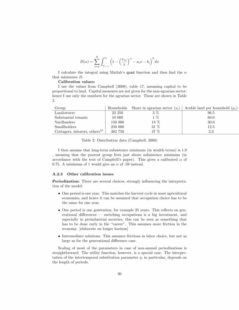
I calculate the integral using Matlab’s quad function and then find the αthat minimizes D.

Calibration values:I use the values from Campbell (2008), table 17, assuming capital to be

proportional to land. Capital measures are not given for the non-agrarian sector;hence I use only the numbers for the agrarian sector. These are shown in Table2.

Group Households Share in agrarian sector (si) Arable land per household (µi)Landowners 22 250 3 % 96.5Substantial tenants 10 000 1 % 60.0Yardlanders 150 000 18 % 30.0Smallholders 250 000 31 % 12.5Cottagers, laborers, others10 382 750 47 % 2.3

Table 2: Distribution data (Campbell, 2008)

I then assume that long-term subsistence minimum (in wealth terms) is 1.9, meaning that the poorest group lives just above subsistence minimum (inaccordance with the text of Campbell’s paper). This gives a calibrated α of0.75. A minimum of 1 would give an α of .59 instead.

A.2.3 Other calibration issues

Periodization: There are several choices, strongly influencing the interpreta-tion of the model:

• One period is one year. This matches the harvest cycle in most agriculturaleconomies, and hence it can be assumed that occupation choice has to bethe same for one year.

• One period is one generation, for example 25 years. This reflects on gen-erational differences — switching occupations is a big investment, andespecially in preindustrial societies, this can be seen as something thathas to be done early in the “career”. This assumes more friction in theeconomy. [elaborate on longer horizon]

• Intermediate solutions. This assumes frictions in labor choice, but not aslarge as for the generational difference case.

Scaling of most of the parameters in case of non-annual periodizations isstraightforward. The utility function, however, is a special case. The interpre-tation of the intertemporal substitution parameter η, in particular, depends onthe length of periods.

30

Scaling: y, k, and l: The production function y = z1−αkαl1−α gives therelationship of the measurements of capital, labor and output. As the laborinput is scaled to 1, the scaling of the other two will have to take this intoaccount. [more on this later. easiest is probably to set Z0 = 1]

Aggregates: Aggregate GDP11 and aggregate capital are relevant for cali-bration.

Output:By the output approach:

Yt = (AC,t)α(Zt(LC,t + LW,t))

1−α + Z1−αt

∑i∈LI

(aαi,t)− δA− (1− ν − δ)AW

(17)

Using instead the income approach, inserting for wt from (11), I can verifythat I get the same result as for the output approach.12

Capital: 13 To calculate for capital-output ratio, first derive the ratio fromEquation (17), assuming that in the long run the number of independents, LI

11As total population is indexed to 1, I do not differentiate between gross and per capitavariables

12

Yt =∑i

(m(ai,t, wt)− ai,t)

=∑i∈LW

(wt + (ν − 1)ai,t) +∑i∈LI

(aαi,tZ1−αt − δai,t) +

∑i∈LC

((1− α)1−αα αZ

1−αα

t w− 1−α

αt ai,t + wt − δai,t)

= (LW,t + LCt )wt + (η − 1)AW,t + Z1−αt

∑i∈LI

aαi,t

− δ(AI,t +AC,t) + (1− α)1−αα αZ

1−αα

t w− 1−α

αt AC,t

Yt = (LW,t + LCt )((1− α)Z1−αt

(AC,t

LC,t + LW,t

)α) + (η − 1)AW,t + Z1−α

t

∑i∈LI

aαi,t

− δ(AI,t +AC,t) + (1− α)1−αα αZ

1−αα

t

((1− α)Z1−α

t

(AC,t

LC,t + LW,t

)α)− 1−αα

AC,t

Yt = (LW,t + LCt )1−α((1− α)Z

(1−α)t (AC,t)

α) + (η − 1)AW,t + Z1−αt

∑i∈LI

aαi,t

− δ(AI,t +AC,t) + (1− α)1−αα αZ

1−αα

t (1− α)−1−αα Z

(− 1−αα

)(1−α)t Aα−1

C,t (LC,t + LW,t)1−αAC,t

Yt = (LW,t + LCt )1−α(1− α)Z

(1−α)t (AC,t)

α + αZ1−αt (LC,t + LW,t)

1−αAαC,t + (η − 1)AW,t + Z1−αt

∑i∈LI

aαi,t

− δ(AI,t +AC,t)

Yt = (LW,t + LCt )1−αZ

(1−α)t (AC,t)

α + (η − 1)AW,t + Z1−αt

∑i∈LI

aαi,t

− δ(AI,t +AC,t)

13Any “capital stock” measure for pre-1850 periods will be highly uncertain, and thatuncertainty is likely to dwarf definition questions about whether aggregate capital shouldequal AC , AC +AI or AC +AI +AW . If I have wealth distribution data for a period I havethis measure directly.

31

will be close to zero, as will the wealth of workers AW . This gives the expressionto calibrate β to a given capital-output ratio in steady state: 14

β =

(α

(ACY

)−1+ (1− δ) + αδ

)−1(18)

A.3 Solution method

Discrete state space. I discretize the state space for individual wealth a, witha large number of discrete points (now. 1024 points). Denote this grid A. I alsodefine a discrete initial distribution of wealth over this space, typically with alarger space between agents.

Defining the long run. I impose that in the long run the wealth of eachgroup should be constant. This follows from the discussion on steady statesabove. Following Auerbach and Kotlikoff (1987) as referred in Heer & Maussner(2009), I set this “long run” as starting at t = T , with T being a sufficientlylarge number.

Initial and end conditions. The wage in the initial period follows fromthe initial distribution. The wage in the end period follows from Equation(12).I then guess a wage path w ≡ {wt}Tt=0 between these points.

Iterative solution. For a given guess w:

• Calculate the long run utility∑∞t=T β

tu(m(a,wLR)− a) for all a ∈ A

• For each period t < T , calculate optimal at+1 at all points in the grid:maxat+1

u(m(at, wt)− at+1) + βV (at+1,w)15

• When all optimal at+1 at all points in the grid have been found, simulatethe path of all agents in the initial distribution from t = 1 to t = T and

14

K

Y=AC

Y=

AC

AαCZ1−α11−α − δAC

=1

Aα−1C Z1−α − δ

Reinserting for AC from Equation (14):

AC

Y=

1β−1−(1−δ)

α− δ

To calibrate β for given capital-output ratio in steady state:

β =

(α

(AC

Y

)−1

+ (1− δ) + αδ

)−1

15explain speedup (use of non-crossing) here

32

keep track of the size of each group and capital stock(LW , LI , LC , AW , AI , AC)in each period

• Calculate the wage in each period using Equation (11) and use this toupdate the wage guess w

Iterate on this until the initial and updated guess are sufficiently close.

A.4 Extension: The model with stochastic returns

[note to reader: I am uncertain of whether this should be in this paper. For thisreason it is placed in the appendix for the time being.]

Up to this point, I have focused on a deterministic model. In this model thereis no relative mobility — as everyone is equal, there is no way to “climb past”someone further up in the wealth distribution. As discussed in the introductorychapter, a framework with idiosyncratic, uninsurable individual shocks is oneway to study economies where agents are mobile.

As the emphasis of the model is on production rather than labor market fric-tions, I will focus on uncertainty in the process of production itself. Concretely,the assumption will be made that each firm receives a idiosyncratic shock to theefficiency parameter Z:

Zi,t = Zt + εi,t (19)

I will interpret this as uneven technological process: while all goods are per-fectly substitutable, each firm is producing different goods with slightly differenttechnologies. While the overall technological trend is deterministic, the exactspeed of progress in any one technology at a given time is stochastic. For thatreason, firms experience random productivity.

To simplify the exposition, I will assume that the capital any individual putsinto storage is of the same type that is used in production. That means thata person that has low Z if choosing to be an entrepreneur in any given periodwill also experience a lower storage return this period.

For simplicity, the realized shock can take one of two values: high or low.This corresponds to aggregate productivity being Zt + εL or Zt + εH , and thestorage return being νL = ν(εL) and νH = ν(εH).

With uncertainty, it becomes most convenient to study the intertemporaldecision using recursive methods. The value function is

V (a, ε;w,Z) = maxa′

(u(m(a, ε;w)− a′) + βE[V (a′, ε′;w′, Z ′)|ε]) (20)

This can then be solved using well-established algorithms. 16

16Pending some proofs that might be needed due to the non-convexity of returns. Thealgorithm is:

33

A.4.1 Equilibrium with stochastic mobility

For low levels of uncertainty, a result similar to the previous sections can beexpected; returns for workers with a good storage shock are not high enoughto make increased saving optimal. However, for some sets of parameters what Iwill term “perfect mobility” will ensue — given an infinitely long strike of goodshocks, the poorest agent will always save, and end up being the richest. Withperfect mobility the final distribution is independent of the initial conditions.

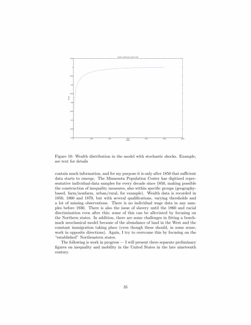
The numerical solution to the nondeterministic problem is work in progress.To illustrate, I give one example of an equilibrium is given in Figure 10. As isevident from the figure, the economy is “split”; around 96% of the populationare workers with zero wealth. The remaining group have a conventional left-skewed wealth distribution.17 The resulting group sizes in this simulation areL1 = 0.9629, L2 = 0.0092, L3 = 0.0279 and the wage level is 1.8390.

B Appendix: Applications

[Note: I am still not sure to what extent I will focus on these issues in themain paper. For that reason these sections are placed in the appendix. Parts ofthe text here is not updated to be in accordance with some of the more recenttheoretical results in the paper. Some of this will be dropped altogether andsome will be extended and included in the main text.]

In this section I discuss some applications of the model. Though evidencefor the overall pattern exists (as discussed in the introduction), I would liketo do a more thorough within-country examination. Unfortunately, data frombefore 1800 (where Figure 1 has its kink) is hard to come by. This section willtry to overcome that difficulty by looking at somewhat more recent data. Istart with some preliminary work on the United States, and go on to discussmore generally the scope for using contemporary developing-country data, andwhether the model can have some application on a global scale.

B.1 A within-country example: United States, 1860-70

The United States is unique in having good data for very early periods, withcensuses being held every ten years since 1790. However, early censuses do not

• Guess a wage w

• Calculate value function V (a, ε) to get optimal savings rule a′(a, ε)

• For a given initial distribution, simulate agents’ behavior until the wealth distributionconverges

• From the resulting ergodic distribution, calculate wnew. Return w − wnew• With the above as the function f(w), search for f(w) = 0

When mobility is not perfect (as discussed in the next paragraph), the result will be depen-dent on the initial distribution (point 3 in the list above).

17The parameters used in this solution are: α = .33, β = 0.9999, η = 2, δ = 0.05, Zl =0.6, Zh = 1.4, νl = 0.85, νh = 0.95. The transition matrix is πii = .7, πij = .3, i, j = {l, h}.The model is simulated on a grid that is uniform on exp(a) with 101 grid points.

34

0 2000 4000 6000 8000 10000 120000.96

0.965

0.97

0.975

0.98

0.985

0.99

0.995

1

1.005

Wealth

Den

sity

Wealth, cumulative plot, dynamic model

Figure 10: Wealth distribution in the model with stochastic shocks. Example,see text for details

contain much information, and for my purpose it is only after 1850 that sufficientdata starts to emerge. The Minnesota Population Center has digitized repre-sentative individual-data samples for every decade since 1850, making possiblethe construction of inequality measures, also within specific groups (geography-based, farm/nonfarm, urban/rural, for example). Wealth data is recorded in1850, 1860 and 1870, but with several qualifications, varying thresholds anda lot of missing observations. There is no individual wage data in any sam-ples before 1930. There is also the issue of slavery until the 1860 and racialdiscrimination even after this; some of this can be alleviated by focusing onthe Northern states. In addition, there are some challenges in fitting a bench-mark neoclassical model because of the abundance of land in the West and theconstant immigration taking place (even though these should, in some sense,work in opposite directions). Again, I try to overcome this by focusing on the“established” Northeastern states.

The following is work in progress — I will present three separate preliminaryfigures on inequality and mobility in the United States in the late nineteenthcentury.

35

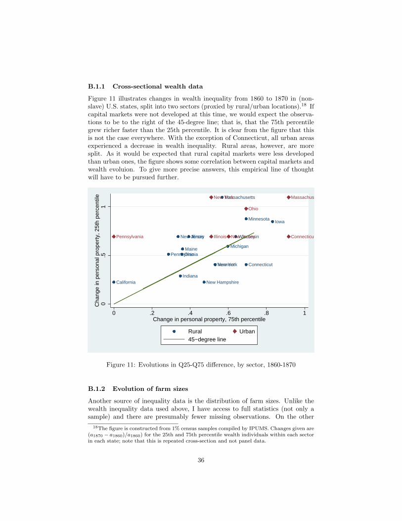
B.1.1 Cross-sectional wealth data

Figure 11 illustrates changes in wealth inequality from 1860 to 1870 in (non-slave) U.S. states, split into two sectors (proxied by rural/urban locations).18 Ifcapital markets were not developed at this time, we would expect the observa-tions to be to the right of the 45-degree line; that is, that the 75th percentilegrew richer faster than the 25th percentile. It is clear from the figure that thisis not the case everywhere. With the exception of Connecticut, all urban areasexperienced a decrease in wealth inequality. Rural areas, however, are moresplit. As it would be expected that rural capital markets were less developedthan urban ones, the figure shows some correlation between capital markets andwealth evoluion. To give more precise answers, this empirical line of thoughtwill have to be pursued further.

Connecticut

Maine

Massachusetts

New Hampshire

Vermont

New Jersey

New York

Pennsylvania

Illinois

Indiana

Michigan

Ohio

Wisconsin

IowaMinnesota

California

Connecticut

Massachusetts

New Jersey

New York

Pennsylvania Illinois

Ohio

0.5

1C

hang

e in

per

sona

l pro

pert

y, 2

5th

perc

entil

e

0 .2 .4 .6 .8 1Change in personal property, 75th percentile

Rural Urban45−degree line

Figure 11: Evolutions in Q25-Q75 difference, by sector, 1860-1870

B.1.2 Evolution of farm sizes

Another source of inequality data is the distribution of farm sizes. Unlike thewealth inequality data used above, I have access to full statistics (not only asample) and there are presumably fewer missing observations. On the other

18The figure is constructed from 1% census samples compiled by IPUMS. Changes given are(a1870 − a1860)/a1860) for the 25th and 75th percentile wealth individuals within each sectorin each state; note that this is repeated cross-section and not panel data.

36

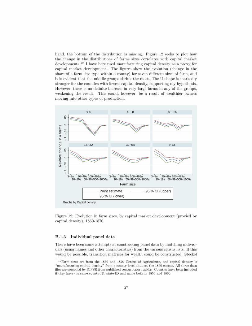
hand, the bottom of the distribution is missing. Figure 12 seeks to plot howthe change in the distributions of farms sizes correlates with capital marketdevelopments.19 I have here used manufacturing capital density as a proxy forcapital market development. The figures show the evolution (change in theshare of a farm size type within a county) for seven different sizes of farm, andit is evident that the middle groups shrink the most. The U-shape is markedlystronger for the counties with lowest capital density, supporting my hypothesis.However, there is no definite increase in very large farms in any of the groups,weakening the result. This could, however, be a result of wealthier ownersmoving into other types of production.

−.1

−.0

50

.05

−.1

−.0

50

.05

3−9a10−19a

20−49a50−99a

100−499a500−1000a

3−9a10−19a

20−49a50−99a

100−499a500−1000a

3−9a10−19a

20−49a50−99a

100−499a500−1000a

< 4 4 − 8 8 − 16

16−32 32−64 > 64

Point estimate 95 % CI (upper)95 % CI (lower)

Rel

ativ

e ch

ange

in #

farm

s

Farm size

Graphs by Capital density

Figure 12: Evolution in farm sizes, by capital market development (proxied bycapital density), 1860-1870

B.1.3 Individual panel data

There have been some attempts at constructing panel data by matching individ-uals (using names and other characteristics) from the various census lists. If thiswould be possible, transition matrices for wealth could be constructed. Steckel

19Farm sizes are from the 1860 and 1870 Census of Agriculture, and capital density is“manufacturing capital density” from a county-level data set the 1860 census. All three datafiles are compiled by ICPSR from published census report tables. Counties have been includedif they have the same county-ID, state-ID and name both in 1850 and 1860.

37

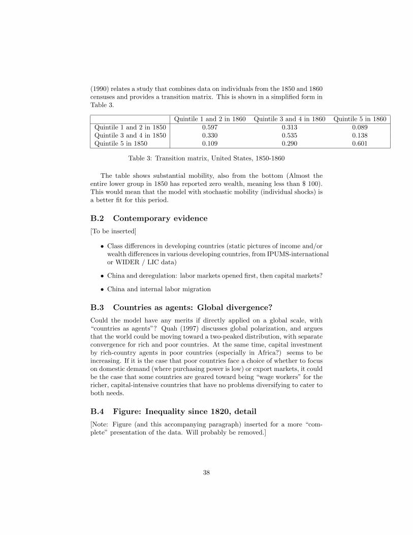
(1990) relates a study that combines data on individuals from the 1850 and 1860censuses and provides a transition matrix. This is shown in a simplified form inTable 3.

Quintile 1 and 2 in 1860 Quintile 3 and 4 in 1860 Quintile 5 in 1860Quintile 1 and 2 in 1850 0.597 0.313 0.089Quintile 3 and 4 in 1850 0.330 0.535 0.138Quintile 5 in 1850 0.109 0.290 0.601

Table 3: Transition matrix, United States, 1850-1860

The table shows substantial mobility, also from the bottom (Almost theentire lower group in 1850 has reported zero wealth, meaning less than $ 100).This would mean that the model with stochastic mobility (individual shocks) isa better fit for this period.

B.2 Contemporary evidence

[To be inserted]

• Class differences in developing countries (static pictures of income and/orwealth differences in various developing countries, from IPUMS-internationalor WIDER / LIC data)

• China and deregulation: labor markets opened first, then capital markets?

• China and internal labor migration

B.3 Countries as agents: Global divergence?

Could the model have any merits if directly applied on a global scale, with“countries as agents”? Quah (1997) discusses global polarization, and arguesthat the world could be moving toward a two-peaked distribution, with separateconvergence for rich and poor countries. At the same time, capital investmentby rich-country agents in poor countries (especially in Africa?) seems to beincreasing. If it is the case that poor countries face a choice of whether to focuson domestic demand (where purchasing power is low) or export markets, it couldbe the case that some countries are geared toward being “wage workers” for thericher, capital-intensive countries that have no problems diversifying to cater toboth needs.

B.4 Figure: Inequality since 1820, detail

[Note: Figure (and this accompanying paragraph) inserted for a more “com-plete” presentation of the data. Will probably be removed.]

38

Figure 13 shows the data from Bourguignon & Morrisson (2002) in moredetail. 20

It is clear that inequality can increase with growth. Going beyond whetherit can, it is interesting to look at the different types of pattern across regions:

For Argentina/Chile, Benelux/Switzerland, Brazil, Cote d’Ivoire/Ghana/Kenya,Italy, Nigeria, North Africa, Scandinavia and the United States the first move-ment in the graph is an increase in inequality over the whole lower 90 %. Itis worth noting the wide selection of countries exhibiting this feature - Scan-dinavia and Brazil are placed at opposite ends of the contemporary inequalityspectrum. For several of these countries inequality decreases in later phases, inaccordance with the overall Kuznets curve hypothesis.

For Australia/Canada/NZ, France, Germany, Korea/Taiwan, Portugal/Spainand UK/Ireland there is a similar movement, but inequality increases mainlyat the top — yielding movements at the top but not at the bottom.

Austria/CZ/Hungary, the Balkan countries, China, Egypt, India, Japan,Poland, Russia, South Africa experience decreasing inequality as the first change,and hence counteract the overall story in this paper. It is worth noting thata majority of these countries have been Communist for long time periods. Forothers I am somewhat uncertain as to whether the figures give accurate repre-sentations — though this objection must of course be raised also for the groupswith increasing inequality.

The remaining countries (Indonesia, Mexico, Philippines/Thailand) are hardto interpret in such a simple scheme.

20The regions “37 Latin American countries”, “45 Asian countries”, “Bangladesh-Pakistan”and “Turkey” are not shown in the figure because they were assumed constant by Bour-gouignon and Morrison, presumably due to insufficient time variation in the sources theyused. The authors make it clear that a lot of assumptions and interpolation underlies thedata; this is also evident for the figure, and the reason for why I show 29 different regions toillustrate the overall point. The upper decile is not shown in the figure for clarity (its share isso much higher than the others and inequality at the top is not a central topic for this paper)

39

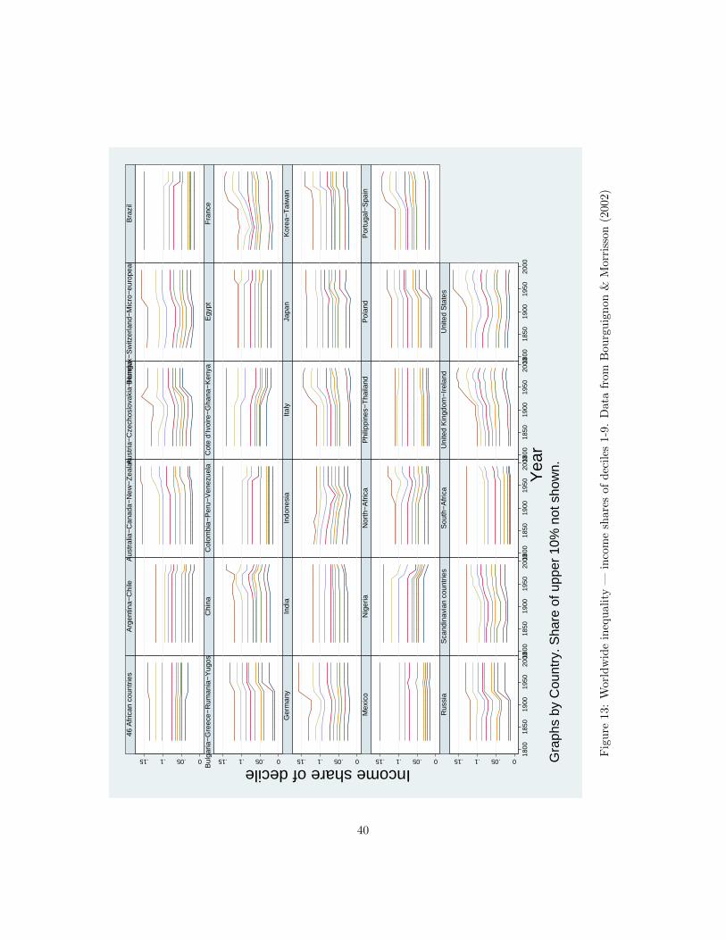
0.05.1.15 0.05.1.15 0.05.1.15 0.05.1.15 0.05.1.15 1800

1850

1900

1950

20001

800

1850

1900

1950

20001

800

1850

1900

1950

20001

800

1850

1900

1950

20001

800

1850

1900

1950

2000

46 A

fric

an c

ount

ries

Arg

entin

a−C

hile

Aus

tral

ia−

Can

ada−

New

−Z

eala

ndAus

tria

−C

zech

oslo

vaki

a−H

unga

ryB

enel

ux−

Sw

itzer

land

−M

icro

−eu

rope

an s

tate

sB

razi

l

Bul

garia

−G

reec

e−R

uman

ia−

Yug

osla

via

Chi

naC

olom

bia−

Per

u−V

enez

uela

Cot

e d’

Ivoi

re−

Gha

na−

Ken

yaE

gypt

Fra

nce

Ger

man

y In

dia

Indo

nesi

aIta

lyJa

pan

Kor

ea−

Tai

wan

Mex

ico

Nig

eria

Nor

th−

Afr

ica

Phi

lippi

nes−

Tha

iland

Pol

and

Por

tuga

l−S

pain

Rus

sia

Sca

ndin

avia

n co

untr

ies

Sou

th−

Afr

ica

Uni

ted

Kin

gdom

−Ir

elan

dU

nite

d S

tate

s

Income share of decile

Yea

rG

raph

s by

Cou

ntry

. Sha

re o

f upp

er 1

0% n

ot s

how

n.

Fig

ure

13:

Wor

ldw

ide

ineq

ual

ity

—in

com

esh

are

sof

dec

iles

1-9

.D

ata

from

Bou

rgu

ign

on

&M

orr

isso

n(2

002)

40

References

Anchorena, Jose, & Modalsli, Jørgen H. 2009. Factor-augmenting technicalchange and the British Industrial Revolution. Working paper.

Banerjee, Abhijit V., & Newman, Andrew F. 1993. Occupational Choice and theProcess of Development. The Journal of Political Economy, 101(2), 274–298.

Bourguignon, Francois, & Morrisson, Christian. 2002. Inequality among WorldCitizens: 1820-1992. The American Economic Review, 92(4), 727–744.

Bourguignon, Francois. 2005. The Effect of Economic Growth on Social Struc-tures. Handbook of Economic Growth, 1(2), 1701–1747.

Campbell, Bruce M. S. 2008. Benchmarking medieval economic development:England, Wales, Scotland, and Ireland, c.1290. The Economic History Review,61(4), 896–945.

Caselli, Francesco, & Ventura, Jaume. 2000. A Representative Consumer Theoryof Distribution. The American Economic Review, 90(4), 909–926.

Chatterjee, Satyajit. 1994. Transitional dynamics and the distribution of wealthin a neoclassical growth model. Journal of Public Economics, 54(1), 97–119.

Collins, Daryl, Morduch, Jonathan, Rutherford, Stuart, & Ruthven, Orlanda.2009. Portfolios of the Poor: How the World’s Poor Live on $2 a Day.Princeton University Press.

Corbae, Dean, D’Erasmo, Pablo, & Kuruscu, Burhanettin. 2009. Politico-economic consequences of rising wage inequality. Journal of Monetary Eco-nomics, 56(1), 43–61.

Galor, Oded, & Moav, Omer. 2006. Das Human-Kapital: A Theory of theDemise of the Class Structure. Review of Economic Studies, 73(1), 85–117.

Galor, Oded, & Zeira, Joseph. 1993. Income Distribution and Macroeconomics.The Review of Economic Studies, 60(1), 35–52.

Galor, Oded, Moav, Omer, & Vollrath, Dietrich. 2009. Inequality in Landowner-ship, the Emergence of Human-Capital Promoting Institutions, and the GreatDivergence. The Review of Economic Studies, 76(1), 143–179.

Garcia-Penalosa, Cecilia, & Turnovsky, Stephen J. 2009. The dynamics of wealthinequality in a simple Ramsey model: A note on the role of production flexi-bility. Macroeconomic Dynamics, 13(02), 250–262.

Ghatak, M., & Jiang, N. 2002. A simple model of inequality, occupational choice,and development. Journal of Development Economics, 69(1), 205–226.

Hansen, G. 1985. Indivisible labor and the business cycle. Journal of MonetaryEconomics, 16(3), 309–327.

41

Harris, John R., & Todaro, Michael P. 1970. Migration, Unemployment andDevelopment: A Two-Sector Analysis. American Economic Review, 60(1),126–142.

Heer, Burkhard, & Maussner, Alfred. 2009. Dynamic General Equilibrium Mod-eling: Computational Methods and Applications. Second edn. Springer.

Hoffman, Philip T., Jacks, David S., Levin, Patricia A., & Lindert, Peter H.2002. Real Inequality in Europe since 1500. The Journal of Economic History,62(2), 322–355.

Krusell, Per, & Rıos-Rull, Jose-Victor. 1999. On the Size of U.S. Government:Political Economy in the Neoclassical Growth Model. American EconomicReview, 89(5), 1156–1181.

Kuznets, Simon. 1955. Economic Growth and Income Inequality. The AmericanEconomic Review, 45(1), 1–28.

Milanovic, Branko, Lindert, Peter H., & Williamson, Jeffrey G. 2007. MeasuringAncient Inequality. National Bureau of Economic Research Working PaperSeries, 13550(October).

Moene, Karl O., & Wallerstein, Michael. 2001. Inequality, Social Insurance, andRedistribution. American Political Science Review, 95(4), 859–874.

Mookherjee, Dilip, & Ray, Debraj. 2003. Persistent Inequality. Review of Eco-nomic Studies, 70(2), 369–393.

Quah, Danny T. 1997. Empirics for Growth and Distribution: Stratification,Polarization, and Convergence Clubs. Journal of Economic Growth, 2(1),27–59.

Ramsey, F. P. 1928. A Mathematical Theory of Saving. The Economic Journal,38(152), 543–559.

Rutherford, Stuart, & Arora, Sukhwinder S. 2009. The Poor and Their Money:Microfinance From a Twenty-First Century Consumers Perspective. Secondedn. Practical Action.

Sokoloff, Kenneth L., & Engerman, Stanley L. 2000. History Lessons: Insti-tutions, Factors Endowments, and Paths of Development in the New World.The Journal of Economic Perspectives, 14(3), 217–232.

Song, Z., Storesletten, K., & Zilibotti, F. 2009. Growing like China. Workingpaper, November.

Steckel, Richard H. 1990. Poverty and Prosperity: A Longitudinal Study ofWealth Accumulation, 1850-1860. The Review of Economics and Statistics,72(2), 275–285.

42

Van Zanden, J. L. 1995. Tracing the Beginning of the Kuznets Curve: WesternEurope during the Early Modern Period. The Economic History Review,48(4), 643–664.

43