Income Redistribution in a Federal System of Governments

Roger H. Gordon, University of California, San Diego Julie Berry Cullen*, University of California, San Diego

ABSTRACT: Though the traditional literature in fiscal federalism argues that the Federal government should have primary responsibility for income redistribution, U.S. states are in fact actively engaged in redistribution. This paper develops a positive model of the respective roles of state and Federal governments that can rationalize this observation. Redistribution by states creates positive horizontal fiscal externalities to other states due to migration, but negative vertical fiscal externalities to the national government due to changes in reported taxable income. We forecast that states will engage in at least some redistribution, though to a lesser degree the greater are mobility relative to taxable income elasticities. The Federal government can then choose the degree of Federal redistribution to assure that the net externalities are zero. Given such policies, we then estimate the welfare weights and migration elasticities for different income groups that would generate the effective net tax schedules observed in the U.S. The parameter estimates are broadly plausible, suggesting that the model can help explain the division of responsibilities for redistribution between state and Federal governments. KEYWORDS: Fiscal federalism; Income redistribution; Fiscal externalities JEL CODES: H2; H7 * Corresponding author. University of California, San Diego, 9500 Gilman Drive, La Jolla, CA, 92093-0508. E-mail addresses: rogordon@ucsd.edu (R.H. Gordon), jbcullen@ucsd.edu (J.B. Cullen).

1

1. Introduction

There is a well-cited literature in public finance that discusses how fiscal functions should be divided among different levels of government.1 The resulting conventional wisdom is that the Federal government should take primary if not sole responsibility for redistribution. The national government does not need to worry about mobility across regions in response to redistribution, while such mobility can seriously hamper redistribution by state and local governments. Given this, why do we see states in the U.S. engaged so actively in redistribution? Most state revenue comes from personal income and sales taxes, rather than from user fees, and a number of key transfer programs are administered at the state level, including Medicaid and TANF.

The objective of this paper is to shift from a normative to a positive perspective. What is the equilibrium allocation of fiscal functions across different levels of government? Using a standard description of the objectives pursued by different levels of government,2 we find that sub-national governments will be actively involved in redistribution regardless of the amount of redistribution undertaken by the national government. Given this inevitability, the national government will choose policies to correct for any deviations between the redistribution already done by the states and the overall amount of redistribution desired.

This limited role for the national government in redistribution is most stark when there are no mobility pressures, the setting we start with in section 2. Here, the Federal government will entirely cede responsibility for redistribution to state governments.3 To see this, consider what happens when the national government chooses any particular tax structure. Taking this policy as given, state governments have an incentive to intervene to redistribute further: at the margin, additional redistribution generates further equity gains while the efficiency costs show up entirely as a drop in Federal tax revenue. If a state is small relative to the nation, then it would ignore these offsetting losses in Federal revenue, and continue to expand redistribution until the equity gains are offset by those efficiency costs reflected in the resulting drop in state revenue due to behavioral responses.

The drop in reported taxable income due to state taxes also reduces Federal revenue, so that there will be excessive redistribution to the extent that the Federal government engages in any redistribution.4 As a result, the Federal government in equilibrium would not choose to redistribute: the extent of redistribution chosen by state governments is also optimal from the national perspective, given the assumed lack of mobility and therefore lack of fiscal externalities to other states.

In section 3, we reexamine the joint choice of redistribution by state and Federal governments when individuals are mobile across states. Now, the equilibrium level of redistribution by state governments will be less than would be chosen if the state governments could coordinate, or if only the Federal government took responsibility for redistribution. In particular, redistribution by a state imposes a positive “horizontal” fiscal externality on other

1 See, for example, Musgrave (1971, 1999), Oates (1972, 1977), and Stigler (1957). 2 The underlying objectives of the national and state governments are assumed to take the same form, though the national government is concerned with the welfare of all residents while each state government is concerned with the welfare of residents in that state. 3 This may, for example, explain the very limited role of the European Union in redistributing income within the EU, deferring instead to member states to engage in redistribution. 4 The presence of negative vertical externalities when multiple levels of government share the same tax base has received considerable attention in the literature (e.g., Keen (1998)), and appears to have been first noted by Flowers (1988).

2

states, due to the emigration of net payers to other states and the immigration of net recipients from other states.5 Counteracting this, it also continues to impose a negative “vertical” fiscal externality on the Federal government to the extent that Federal taxable income falls. If these positive horizontal and negative vertical externalities just offset, through the judicious choice of the extent of Federal redistribution, then the equilibrium outcomes are in fact jointly optimal.

The most closely related analysis to ours, Boadway et al. (1998), solves for the optimal use of a linear income tax by both state and national governments. Like us, the authors find that without mobility the Federal government will defer to state governments to handle redistribution, and with mobility will set policy so that vertical and horizontal externalities just offset. They, however, do not make much progress in characterizing the resulting Federal policies: the Federal government is assumed to have few instruments available, but faces potentially different migration responses for individuals with different incomes. Our paper differs in that we allow governments to make use of non-linear tax schedules, creating enough policy flexibility to address the potential variety of migration responses and yielding easily interpreted expressions for the resulting equilibrium policies for both state and Federal governments. We are then able to take the model to the data to evaluate its practical import.

In section 4, we use the framework and estimates in Gruber and Saez (2002) to infer the model parameters needed to rationalize the observed overall state plus Federal redistribution and the observed composition of state vs. Federal redistribution.6 Gruber and Saez (2002) characterize the optimal extent of redistribution considering only one level of government, which is implicitly the combined equilibrium redistribution undertaken by all levels of government in our extended framework. We take as inputs their estimates of the taxable income elasticities and the observed Federal and state tax schedules across each of five tax brackets for joint filers in 1990. The brackets and year are chosen to match their analysis, and we account for state sales taxes and Federal and state assistance programs in addition to Federal and state income taxes in calculating the effective net tax schedules. Using our formulas for the equilibrium tax schedules, we then solve for the welfare weight and migration elasticity within each bracket that would generate the observed schedules. The welfare weights are pinned down by the combined schedules, and the migration elasticities are then identified from comparing the state and Federal schedules.

The inferred parameters seem broadly plausible, suggesting the model does help explain the respective roles of different levels of government in income redistribution. The resulting welfare weights imply that a dollar to the bottom group provides as much welfare as two dollars in tax revenue, while a dollar to the richest group provides only as much welfare as one-half dollar in tax revenue. We infer very high migration elasticities in the two highest income brackets, and very low elasticities in the bottom three brackets—a pattern that is broadly consistent with migration propensities for different skill groups (U.S. Census, 2003).

The above analysis of shared responsibility for redistribution applies in a closely parallel fashion to a variety of other policies jointly chosen by state and Federal governments. Section 5 5 These horizontal externalities have also been well recognized in the literature. Most relevant to us, Wildasin (1991) characterizes the optimal use of Pigovian subsidies in addressing horizontal externalities from state redistribution, but in a setting without vertical externalities, so one in which states would not in fact choose to redistribute given optimal Federal redistribution. Other papers that solve for optimal Pigovian subsidies to address various interstate spillovers include Boadway and Hayashi (2001), Bucovetsky and Smart (2006), Buettner (2006), Dahlby (1996), Esteller and Sole (2002), Gordon (1983), Inman and Rubinfeld (1996), and Köthenbürger (2002). 6 For another recent attempt to infer welfare weights from estimated labor supply elasticities and observed tax rates, see Bargain et al. (2011).

3

provides a brief sketch of a general model determining when government functions are pursued only by the Federal government, only by state governments, or by both levels of government. Finally, section 6 provides some brief conclusions. 2. Equilibrium redistribution in a Federal system with no mobility

We begin by laying out the general assumptions of the model. We then derive state and Federal redistribution policies when people do not relocate in response to these policies. In the next section, we reexamine these policies when relocation can occur. 2.1 Basic assumptions of the model

Assume that state governments and the Federal government share the same form of objective. In particular, the state government chooses policies to maximize the sum of individual utilities of residents in the state, while the Federal government chooses policies to maximize the sum of individual utilities of residents in the nation as a whole. The key assumption is that government policy is Pareto optimal, so that all feasible opportunities are used to aid some individuals with no harm to others. We make no assumptions about relative welfare weights, allowing the government’s perceived social marginal utility of income to vary arbitrarily with income.7

The national population is N, while the population of state s is denoted by

€

ns . Individuals differ in skill levels, denoted by their wage rate w. The national marginal distribution function for wage rates equals

€

f (w) with

€

∫ f (w)dw = N , and equals

€

∫ fs(w)dw = ns in each state s. To simplify the analysis, we will later impose the assumption that all states are identical, implying the same population n in each state as well as

€

fs(w) = nf w( ) N . For now, though, we allow for heterogeneous states.

We take relative wage rates as fixed throughout the analysis.8 One common assumption justifying fixed relative wage rates is that workers with different skill levels are perfect substitutes in production, with the skilled simply providing more labor input per hour than the less skilled. Even if workers are not perfect substitutes in production, though, we still would predict fixed relative wage rates under the assumptions used in the Heckscher-Ohlin model. In particular, factor prices in a state are equalized to those prevailing in the national market if the optimal skill composition within an industry given these national factor prices differs enough by industry, there are at least as many industries as there are skill types, and the actual skill composition of workers is in the span of optimal skill compositions across industries. State policies affect industrial composition, but relative wages are determined by the set of equilibrium output prices in the national market.

Each government is assumed to have available the same set of policies. Each is choosing a personal income tax schedule equal to

€

TF (y) for the Federal government and

€

Ts(y) in each state,

7 The political economy literature has developed models that generate such an objective function, by assuming probabilistic voting and a desire by politicians to maximize their vote shares. For a general discussion of these voting models, see Hettich and Winer (1999) and Lindbeck and Weibull (1987). These models forecast greater welfare weights for those whose votes are more affected by alternative policies. Chen (2000) provides an application of these results to the political choice of the overall tax schedule. 8 Though theoretical support for this assumption seems strong, we should note the conflicting claim in Feldstein and Wrobel (1998) that state income taxes are fully offset by changes in pre-tax wage rates.

4

where

€

y = wL(w) denotes an individual’s labor income and

€

L(w) her labor supply.9 The resulting revenue is used to finance lump-sum transfers

€

aF and

€

as by the Federal and state governments, respectively. Budget balance then requires that

€

∫TF wL(w)( ) f (w)dw = NaF for the national government and

€

∫Ts wL(w)( ) f s(w)dw = nsas for state governments.10 We assume that each state is small enough that it ignores the effects of its decisions on

Federal tax revenue and policy. Each state receives too small a fraction of extra Federal revenue to matter, and its policies affect too small a fraction of national residents to have a noticeable effect on Federal tax policy.11 The Federal government, though, needs to take into account not only how individuals but also how state governments respond to Federal policy choices. Formally, we therefore assume that the Federal government is a Stackelberg leader, setting its tax policy first while taking into account how state governments respond.12 2.2 Optimal overall tax schedule

Before we examine the policy choices by state and Federal governments, we first examine the optimal choice of overall redistribution from the perspective of the national government as context. Consider the choice of

€

a = aF + as and

€

T (y) = TF (y) + Ts(y). If the national government controlled both tax schedules, it would choose the overall tax schedule to maximize13

€

∫U wL −T (wL) + a,L( ) f (w)dw (1)

We characterize the optimal tax schedule following the logic in Saez (2001). Begin by mapping the original distribution of skill levels into the distribution of pretax income arising under the optimal policies. The resulting density is denoted

€

g(y), and the implied cumulative distribution is denoted

€

G(y) . The government budget constraint can be expressed by

€

∫ T (y) − a( )g(y)dy = 0, with an associated Lagrangian multiplier of

€

λ . Assuming based on the empirical evidence in Gruber and Saez (2002) that there are no

income effects on labor supply, the first-order condition for the lump-sum grant a is

€

v(y)g(y)dy0

∞

∫ = Nλ , or

€

ω(y)g(y)dy0

∞

∫ = N (2)

9 For simplicity we assume that y is non-negative, ignoring for example losses among the self-employed. 10 For now, we assume that these lump-sum transfers are in cash, but discuss below how results change when each government can make transfers either in cash or in kind (through public services). 11 We implicitly assume that the Federal tax schedule does not vary depending on state of residence. While we know of no examples of national tax schedules varying by state, intergovernmental transfers certainly do. We will briefly discuss below the possible role of such state-specific transfers. 12 Equilibrium policies would be unchanged if we instead assumed a Nash equilibrium, in which both Federal and state governments take policies elsewhere as given when setting their own policies. To see this, note that the Federal government is maximizing an implicit objective function

€

W (F,S(F)) over Federal policies F under a Stackelberg equilibrium, where S is the resulting state policies, whereas it is maximizing

€

W (F | S) in a Nash equilibrium. For any given S, the choice for F is the same in the two cases if

€

∂W /∂S = 0 at the equilibrium. This condition holds in our setting since, at the optimal Federal policies, state choices generate no net externalities. 13 Results would be the same if, instead of an additive function, we specified a general Bergsonian welfare function

€

W ({U h}) . The marginal utility of income of individual h would simply be reinterpreted to equal

€

Whvh(y) .

5

Here,

€

v(y) denotes the marginal utility of income for those with income level y,14 while

€

ω(y) is the marginal utility of income relative to the welfare value of additional tax revenue. Under the optimal policies, the welfare value of the marginal dollar of revenue equals the average marginal utility of income across individuals.

We can characterize the optimal schedule of marginal tax rates by calculating the impact of a perturbation to the schedule for T, recognizing that the change must leave social welfare unaffected starting from the optimal tax schedule. Consider raising the marginal tax rate by

€

dT over the interval z to

€

z + dz. This tax change is equivalent to a lump sum tax of

€

dTdz on the

€

N −G(z) individuals earning at least

€

z + dz, leading to a loss in utility for those individuals and a gain in revenue for the government. In contrast, those earning less than z are unaffected by the tax change. However, the

€

g(z)dz individuals with incomes between z and

€

z + dz now face a higher marginal tax rate, inducing a drop in their labor supply and a resulting loss in tax revenue.15 This loss in tax revenue varies directly with the elasticity of labor supply with respect to the after-tax wage rate for individuals with labor income of z, which we denote by

€

ε(z) .16 The initial tax schedule is optimal if these three welfare effects sum to zero, implying that

€

− v(y)g(y)dy + λ N −G(z)( )z

∞

∫ − λ ʹ′ T (z)1− ʹ′ T (z)

ε (z)zg(z)⎡

⎣ ⎢

⎤

⎦ ⎥ × dTdz = 0 (3)

Simplifying, we find the following expression determining the optimal overall marginal tax rate at any income level z:

€

ʹ′ T (z)1− ʹ′ T (z)

=N −G(z)( ) 1−ω (z)( )

ε(z)g(z)z (4)

Here,

€

ω (z) ≡ ωz

∞

∫ (y)g(y)dy / N −G(z)( ) is the average relative marginal utility of income for all

those with income above z. Note that equation (2) implies that

€

ω (0) =1. The expression in equation (4) reflects the classic tradeoff between the equity gains and

efficiency costs of taxation.17 Assuming that the marginal utility of income declines with income,

€

ω (z) is also a declining function of z, with

€

ω (z) <1 for

€

z > 0. The equity gains then depend on

14 Starting from the utility function

€

U (C, y /w) , individuals maximize this utility subject to their budget constraint

€

C = y −T (y) + a . The marginal utility of income is defined to equal the value of the Lagrangian multiplier on this budget constraint, which also equals the marginal utility of consumption. 15 Labor supply changes continuously with the tax rate, as we assume, as long as the initial budget constraint is concave throughout (or at least less convex than the indifference curves). If there are discrete changes in tax rates at some level of income, though, as might occur when the population density is not smooth, then individuals with different wage rates may bunch at a kink point in the tax schedule.

16 This loss is equal to

€

ʹ′ T (z) ∂z∂ ˜ w

×∂ ˜ w

∂ ʹ′ T (z)⎛

⎝ ⎜

⎞

⎠ ⎟ dTg(z)dz , where

€

˜ w ≡ w(z) 1− ʹ′ T (z)( ) is the after-tax wage rate.

Expanding yields

€

ʹ′ T (z) ∂z∂ ˜ w

ט w z

⎛

⎝ ⎜

⎞

⎠ ⎟

z˜ w ×

∂ ˜ w ∂ ʹ′ T (z)

⎛

⎝ ⎜

⎞

⎠ ⎟ dTg(z)dz =

ʹ′ T (z)1− ʹ′ T (z)

ε (z)zg(z)dTdz .

17 Note that redistribution will never be complete, since as incomes become more equal the marginal equity gains from further redistribution go to zero but the marginal efficiency costs grow with the tax rate.

6

the value of the extra tax revenue compared to the average foregone utility among those paying the extra lump-sum tax,

€

1−ω (z) , times the number of people,

€

N −G(z), paying the extra lump-sum tax. The efficiency costs of taxes are captured by the denominator in this expression: the more elastic the labor supply, the greater the number of people affected by the tax change, and the higher their incomes, the larger are the efficiency costs generated by tax distortions and the lower optimal tax rates will be. The relative importance of the equity and efficiency terms depends on the shape of the income distribution, as captured by the ratio

€

N −G(z)( ) g(z)z( ). Diamond (1998) argues that the optimal tax rates will tend to have a U-shaped pattern, reflecting the implications of the hump-shaped distribution of

€

g(z) for the distribution of this ratio. Two commonly cited results in this literature are that the optimal tax rate at the lowest level

of income (Seade (1977)) and the highest level of income (Sadka (1976)) are both zero. With nonzero and finite minimum and maximum income levels, both conditions hold in the above expression.18 However, consistent with the data, we assume that some individuals choose not to work, simply consuming their lump-sum transfer, and assume that incomes can be arbitrarily large. With these assumptions, optimal tax rates will be positive at all positive levels of income. 2.3 Optimal state tax schedules without mobility

What redistribution will each state choose, taking as given the tax policies in other states and also the Federal income tax schedule? Each state maximizes the sum of utilities of state residents subject to the state’s budget constraint,

€

∫ Ts(y) − as( )gs(y)dy = 0 . Retracing the steps in the preceding section using the state’s objective and budget constraint in place of the national versions, we find that the condition characterizing the state’s optimal schedule for an arbitrary Federal schedule equals

€

Tsʹ′(z)

1− ʹ′ T (z)=

ns −Gs(z)( ) 1−ω s(z)( )ε s(z)gs(z)z

(5)

One important implication of equation (5) is that state tax rates are positive, regardless of the Federal tax schedule, since all of the terms on the right-hand side of this equation are positive. The equilibrium does not involve just the Federal government participating in redistribution, contrary to the conventional wisdom.19

This observation also rules out an equilibrium in which the Federal government itself undertakes the overall optimal amount of redistribution. In response, states would redistribute further according to equation (5), so that redistribution will be excessive from a joint perspective. The problem is that the states ignore the impact of their redistribution on Federal tax revenue, trading off the marginal equity gains from further redistribution with the offsetting losses in state revenue due to the resulting behavioral responses. However, the same behavioral changes also result in a loss in Federal revenue, creating a “vertical” fiscal externality, a loss ignored by each state since that state’s residents bear a negligible fraction of this loss. In particular, to measure all of the efficiency costs of the change in the marginal tax rate in any given tax bracket, the 18 At the minimum income

€

ymin ,

€

ω (ymin ) =1, while at the maximum income

€

N −G(ymax ) = 0 , in both cases leading to a zero optimal tax rate according to equation (4). 19 Johnson (1988) appears to have been the first to note that states have an incentive to engage in income redistribution, given the resulting negative vertical fiscal externalities, at least when there is no migration.

7

numerator on the left-hand side of equation (5) would need to be

€

ʹ′ T (z) rather than just

€

Tsʹ′(z) .

Note that optimal tax schedules can vary across states for a number of reasons. For one, differences in the income distribution across states enter in multiple ways in equation (5), affecting in particular the fraction of people paying an extra lump-sum tax (

€

ns −Gs(z)) and the fraction facing more distorted marginal incentives (

€

gs(z) ) when the marginal tax rate is changed in any given tax bracket. Differences in the income distribution also affect the average marginal utility of those paying the extra lump-sum tax,

€

ω s(z) , as would any differences in welfare weights across states. Finally, the elasticity of labor supply (

€

εs(z)) could in general vary by state, due for example to differences in the types of jobs or in patterns of monetary vs. non-monetary compensation across states.20 2.4 Optimal Federal tax schedule without mobility

We next consider the choice of Federal tax schedule given how states choose their own tax schedules. To simplify the discussion of optimal Federal policy, we assume that states are fully symmetric, implying for example the same income distribution across states and the same labor supply elasticities.

Given symmetry, we easily find that if there is no Federal redistribution at all, then the state’s optimal redistribution is optimal overall, since equation (5) then replicates equation (4). Intuitively, when there is no migration and no Federal taxation, the state is maximizing national utility in choosing its tax policies, since its choices generate no fiscal externalities. Anticipating these optimal policies, there is no need for Federal intervention.

Proceeding more mechanically, for any given tax schedule chosen by the Federal government, equation (5) characterizes the resulting state tax schedule. The objective of the Federal government is then to choose the Federal tax schedule so that the overall tax schedule satisfies equation (4). Since

€

ʹ′ T (y) = TFʹ′(y) + Ts

ʹ′(y), we can subtract equation (5) from equation

(4) to find that

€

TFʹ′(y) = 0: it is optimal for the Federal government to cede full responsibility to

states for redistribution if there is no migration. How would the Federal government respond instead if states are heterogeneous? Here, the

answer depends on the source of heterogeneity. If states simply differ in their populations, nothing changes. If states instead differ in their labor supply elasticities, then states adjust their tax schedules in response. As long as the Federal government cannot differentiate tax schedules by state, then states on their own do better and, as above, the Federal government would not make use of an income tax. However, if the Federal government can make state specific lump-sum transfers,21 then it would do so. The aim would be to target transfers so as to increase tax rates in states where labor supply elasticities are low and decrease them in states where these elasticities are high, in order to reduce the overall efficiency costs of redistribution.

What if states simply differ in their local price level, but not in their distributions of real income? States would then all adopt the same tax schedule on real incomes, a schedule that the Federal government could not replicate. Again, the Federal government fully cedes responsibility

20 While we do not attempt it in this study, it would be of interest to see to what degree differences in state tax schedules can be explained by each of these sources of heterogeneity across states, including as well differences in the migration elasticities introduced in the next section. 21 These can involve differential intergovernmental grants to states rather than differential transfers to households.

8

for redistribution to the states. There would be no grounds in this case for intergovernmental grants.

When differences in the income distribution (or welfare weights) in each state are the reason for different choices for the states’ tax schedules, how would the Federal government respond? Tax rates on high income residents in wealthy states will likely be too low from a national perspective, as will net transfers to poor residents in poor states. Now, the Federal tax schedule responds to the “average” state schedule. Since some states have rates exceeding the rate desired by the national government and some have rates that are too low, the average could well be close to the desired level, still leaving little role for a Federal income tax. However, if Federal lump-sum transfers can vary by state, there would be a role for transfers from high income to low income states. Another possible federal response would be a constitutional mandate prohibiting redistributive taxation at the state level, with all redistribution occurring through the Federal government. 3. Equilibrium redistribution in a Federal system with mobility

How do the above results change when we allow for mobility of residents across states? To begin with, the overall optimal policies do not change at all, at least if we ignore international migration so that policy choices do not affect the national distribution of skill types. State policies do change, however, and this will induce a change in Federal policies. States now affect one another, since changes in state tax structures induce migration across state lines. A higher tax rate within a state will induce some of those paying the extra taxes to leave, and will induce some of those who would be eligible for the extra transfers to relocate to the state.

When making policy choices, we assume that states take as given the policies chosen by other states as well as the Federal tax schedule. We also assume that the objective function of each state depends on the welfare of the residents living in the state at the time the policy is under consideration.22

In order to model explicitly the factors determining household location, assume that the utility of any individual equals

€

˜ γ s U (C,L) if the individual locates in state s.23 Here,

€

˜ γ s is an idiosyncratic taste parameter, drawn from a distribution

€

Γs(γ) .24

3.1 Optimal state tax schedules given mobility

Begin by considering the first-order condition for a state’s lump sum transfer. Any increase in

€

as again provides utility benefits to all residents and costs the government in proportion to the size of the local population. In addition, it now induces migration at a net cost in government

22 In particular, we assume that the set of people entering the government’s objective function does not change in response to a possible policy change, even though there is migration in and out of the state. A complication we then ignore is that the population relevant for future policy decisions is affected by current decisions. See Epple and Platt (1998), Epple and Romer (1991), and Hamilton and Pestieau (2005) for examples of analyses that take account of this endogeneity in the population whose welfare enters the government’s objective. 23 Mansoorian and Myers (1993) appears to be the first study to have used this approach to capture variation in mobility propensities. 24 One special case has everyone receiving the same utility regardless of which state they locate in. Then a state’s population is infinitely elastic—to attract any residents it must offer the highest utility available in any other state. Another special case has extremely diverse tastes and almost no migration in response to policy changes.

9

revenue of

€

Ts(y) − as( ) ∂gs(y) ∂as( )0

∞

∫ dy . Attracting net payers is a fiscal benefit, and conversely

attracting net recipients is a fiscal cost. Combining terms, the resulting first-order condition is:

€

vs(y)gs(y)dy0

∞

∫ − nsλs + λsTs(y) − as

Is(y)ηs(y)gs(y)dy

0

∞

∫ = 0 (6)

Here,

€

Is(y) measures the individual’s net income in state s,

€

ηs(y) denotes the elasticity of the number of individuals at any given level of income in the state with respect to the size of their net income, and is the Lagrangian multiplier on the state’s budget constraint. At least if migration elasticities do not vary with income, the migration term will be negative, making a lump sum transfer more expensive due to the disproportionate in-migration of those with low skills, who impose a net fiscal burden.25

Let

€

M s(z) ≡Ts(y) − as

Is(y)ηs(y)gs(y)dy / ns −Gs(z)( )

z

∞

∫ measure the weighted average impact of

migration on the budget for individuals with incomes above z. Also denote the average marginal

utility of income for all those with income above z by

€

v s(z) ≡ vsz

∞

∫ (y)gs(y)dy / ns −Gs(z)( ) .

Equation (6) then implies that

€

λs = v s(0) / 1− M s(0)( ) . Since

€

M s(0) < 0 is expected, the average marginal utility of income across residents now exceeds the welfare value of additional state revenue. The marginal value of revenue is lower under the optimal policies in the presence of migration because distributing these revenues has negative feedback effects on the budget.

Consider next the expression characterizing the welfare effects of a perturbation in marginal tax rates in the interval z to

€

z + dz. This tax change imposes a lump-sum tax on those with incomes above z, inducing migration for this subset of residents. This migration generates a

revenue loss proportional to

€

Ts(y) − as

Is(y)ηs(y)gs(y)dy

z

∞

∫ , which simplifies to

€

ns −Gs(z)( ) M s(z) .

Solving for the optimal tax rates, now including the migration-induced revenue cost and recalling that

€

ω s(z) ≡ vs(z) /v s(0) given our prior normalization, we find that

€

Tsʹ′(z)

1− ʹ′ T (z)=

ns −Gs(z)( ) 1−ω s(z) 1− M s(0)( ) − M s(z)[ ]ε s(z)gs(z)z

(7)

Relative to the situation without migration, there are two new terms. The first,

€

ω s(z)M s(0) , captures the net revenue loss due to the immigration resulting from a higher lump-sum transfer.26 The other,

€

−M s(z), captures the net revenue loss due to the resulting emigration of those with

25 While

€

∫ Ts(y) − as( )gs(y)dy = 0 , the term in equation (6) weights those with low net income more heavily, and

these are the individuals for whom

€

Ts(y) − as < 0 . 26 In particular,

€

ω s(z) measures the size of the extra lump-sum transfer due to the marginal tax change, as this extra transfer is set equal to

€

ω s(z) under the optimal polices. Per dollar of transfer, the resulting revenue loss due to immigration is measured by

€

M s(0) .

10

incomes above z who now face higher state tax payments. Together, these new terms reduce tax rates at all positive incomes. Their net effect is larger the higher the income.27

Ignoring migration, state tax rates are positive, as is clear from inspection of equation (5). Intuitively, if any marginal tax rate is negative, then raising this tax rate towards zero and then reducing a positive tax rate at a lower level of income so as to preserve overall tax revenue creates both equity and efficiency gains. With migration, there is no longer an assurance that marginal tax rates are positive. Now, raising a negative tax rate towards zero and reducing a positive tax rate at a lower level of income together result in adverse migration effects. More formally, there is no guarantee that the two new migration terms, that together lower optimal rates, are smaller in absolute value than

€

1−ω s(z) . Even with these migration terms, we still conclude that states will always engage in some

redistribution, regardless of the amount of Federal redistribution. If, to the contrary, they engage in no redistribution, then the migration terms are zero, leaving a net welfare benefit from raising marginal tax rates at each income. Redistribution takes place to take advantage of these equity gains until the offsetting efficiency losses due to migration and labor supply responses are weighted by high enough tax rates that these efficiency costs just offset the equity gains. 3.2 Optimal Federal tax schedule given mobility

In order to characterize Federal policy, we again make the simplifying assumption that states are fully symmetric. Therefore, if all states choose the same tax policy, the equilibrium will result in an equal division of each skill group across states. However, if any state deviates from the common tax policy, shifting towards more redistribution, then some of the rich will leave and some of the poor will enter. A sufficient condition for a symmetric equilibrium in which all states adopt the same tax structure, characterized by equation (7), is that the solution to this equation is unique for any given policies in other states. We proceed assuming such a unique solution.

Given the state policies forecast by equation (7), we can proceed mechanically as we did without migration to derive an equation characterizing the optimal Federal tax rate at any given income level by subtracting equation (7) from equation (4). We now find that

€

TFʹ′(z)

1− ʹ′ T (z)=

N −G(z)( )[M (z) −ω (z)M (0)]ε (z)g(z)z

(8)

The numerator in equation (8) measures the positive horizontal externalities provided to other states when state s raises the marginal tax rate at income level z, due to the out-migration from state s of those facing higher tax payments (as measured by

€

M (z)) and the in-migration to state s of those now receiving a larger transfer (as measured by

€

ω (z)M (0)). At the optimal Federal policy, these positive horizontal externalities will just equal the negative vertical fiscal externality generated by the resulting fall in labor supply times the Federal marginal tax rate (as measured by the denominator times the left-hand side of equation (8)).28 27 The combined term

€

ω s(z)M s(0) − M s(z) equals zero at

€

z = 0, and declines with income if

€

ω s '(z) < 0 and

€

M s '(z) > 0 . The latter holds if the net tax grows as a fraction of income as z increases and if migration elasticities do not fall with income. 28 Wilson and Janeba (2005) note that this result of exactly offsetting horizontal and vertical externalities under

11

While the migration response lowered state tax rates, these terms raise Federal tax rates, since

€

M (z) > M (0) and

€

ω z( ) <1. The migration expression grows with z, in itself leading to a progressive Federal schedule with increasing marginal tax rates. The larger are migration effects, the smaller are state tax rates relative to Federal rates. As the migration elasticity increases without bound, state tax rates shrink towards zero,29 so that only the Federal government engages in redistribution. But conversely, we know from the prior section, that if the migration elasticities equal zero, then Federal rates equal zero.

As in the case without mobility, any heterogeneity across states affects the choice of Federal tax policy, with specific results depending on the source of this heterogeneity. The one source of heterogeneity we did not discuss before is differences in migration elasticities. In states with higher migration elasticities at any given income level, horizontal externalities are larger.30 In principle, therefore, the optimal Federal income tax schedule should vary by state. 3.3 Omitted issues

To keep the above discussion as transparent as we could, we omitted a variety of complications. In this subsection, we briefly comment on two.

3.3.a Optimal Federal use of Pigovian subsidies given mobility We assumed above that the only tool available to the Federal government to address

horizontal externalities across states was a Federal income tax. In the setting with symmetric states, the Federal government could achieve its overall desired outcome (as characterized by equation (4)) with this policy, so there was no welfare loss from this restriction in the set of tools. Nonetheless, the Federal government could also address these horizontal externalities generated by state redistribution through use of Pigovian subsidies encouraging redistribution by states. Within our current setting, there would exist a subsidy schedule as a function of income that would also be sufficient in itself to fully internalize the horizontal externalities across states. For any arbitrary schedule of Pigovian subsidies, there is a suitable choice for the Federal income tax schedule that again generates the overall desired redistribution.31

When states are heterogeneous, though, the two policies are no longer perfect substitutes. Consider for example the case when migration elasticities differ by state, e.g. those who choose to live in New York City or California may be very reluctant to leave, but those in some other states may quickly relocate in response to changes in their after-tax income. A uniform Federal income tax cannot fully address these differences in the fiscal spillovers generated in different states. However, a subsidy rate that declines with the amount of state income tax payments at any given income level has the potential to do better.32 In particular, states where there is less of a optimal policies no longer holds when countries compete for a mobile tax base. While their focus was a tax on capital, the same argument applies to taxes on labor income when movement of labor across borders is allowed. 29 As migration elasticities increase without bound, the net tax

€

Ts(y) − as must shrink towards zero for equation (7) to hold. For redistribution to shrink toward zero at all income levels, marginal tax rates must also. 30 Brülhart and Jametti (2006) attempt an empirical test of the relative importance of horizontal vs. vertical externalities in Switzerland. Their key assumptions are that smaller jurisdictions face more pressures from mobility, leading to lower tax rates, but bear a smaller fraction of any resulting drop in Federal revenue, leading to higher tax rates. They find that smaller jurisdictions tend to have higher tax rates. 31 See Sato (2000) for a recognition of this redundancy in policies. 32 The U.S. has a version of this through the implicit cap on itemized deductions for state and local tax payments

12

migration response will choose higher tax rates, and generate smaller externalities at the margin. Their residents would then face the desired smaller marginal subsidy rate if the subsidy rate declines with the size of state income tax payments.

3.3.b Transfers in kind as well as in cash So far, we have assumed that both state and Federal tax revenue is fully paid out in the form

of lump-sum cash transfers. How do results change when we recognize that governments can use revenue to finance both cash transfers and public services? Consider that transfers can be in cash, c, or in kind as government expenditures per capita on socially provided private goods, e, where

€

aF = cF + eF and

€

as = cs + es. Given overall tax revenue, we now face an added choice for each level of government between transfers in cash or in kind.

If the dollar value of public services is the same for all residents,33 the above results are unaffected. In particular, assume that the dollar value of the combined transfers equals

€

cF + cs +κ(es,eF ) . In this case, each government provides services so that

€

κ i ≡ ∂κ(es,eF ) ∂ei =1, with all remaining revenue paid out as cash-transfers, or any deficit financed with a lump-sum tax.

What if the dollar value of public services,

€

cF + cs +κ y(es,eF ), varies with income? From the Federal perspective, optimal service provision for either or is characterized by

€

v(y)g(y)dy = v(y)κ iyg(y)dy

0

∞

∫0

∞

∫ (9)

Here, the weighted average dollar benefit from public services still equals a dollar, with weights equal to the marginal utility of income.

Each state, though, needs to take into account the implications for mobility when deciding on public service provision. The state’s optimal service provision is characterized by

€

v(y)gs(y)dy = v(y)κ sygs(y)dy

0

∞

∫0

∞

∫ + λsTs(y) − as

Is(y)η(y)(κ s

y −1)gs(y)dy0

∞

∫ (10)

From a Federal perspective, states provide too many public services benefiting higher income residents, and too few benefiting poorer residents, due to mobility pressures.

How should the Federal government best respond to these misallocations? We comment only briefly here, since this question goes beyond the intended focus of our paper. If Federal and state expenditures are substitutes, then the Federal government should focus its expenditures on services benefiting primarily the poor. Alternatively, the Federal government can implement matching subsidies for expenditures on services benefiting the poor or mandate state spending on services benefiting the poor. One way to discourage services benefiting the rich is to provide subsidies for lump-sum cash transfers, favoring cash subsidies over those public services not qualifying for explicit subsidies.

because these deductions are not allowed under the Alternative Minimum Tax. 33 For example, if public services are perfect substitutes for privately available goods, then the value of

€

ei equals the cost of the equivalent private goods for all residents.

13

4. Solution for key parameters, given observed policies

In this section, we show how the observed state and Federal tax structures can be used to solve for both the distributional tastes and the migration elasticities that would generate the observed policies. These estimates can serve to assess the plausibility of the above model for the behavior of governments. For example, the inferred migration elasticities can be compared with the admittedly limited empirical evidence on these elasticities to judge whether they seem reasonable. The inferred distributional weights can similarly be compared with those implied by conventional specifications for the utility function, again to judge plausibility.

In estimating these parameters, we build on the procedure used in Gruber and Saez (2002). First, we consider five brackets for the income tax schedule, corresponding to the four taxable income intervals used in their study,34 plus a fifth category for those who currently owe no personal income taxes. Second, we make use of their estimates for the elasticity of taxable income in the top three tax brackets of 0.284, 0.265, and 0.484,35 and follow their assumption for remaining individuals by using the estimate from Moffitt (1992) of 0.4 for the labor supply elasticity of individuals in the bottom two brackets.36

We next need to measure the combined actual (average) state and Federal tax schedules, focusing on 1990 to correspond to the figures used in Gruber and Saez (2002). Our estimation sample is a nationally representative sample of tax-filers and non-filers for that year drawn from the Statistics of Income individual tax returns and Current Population Survey, respectively. We limit the sample to nonelderly married couples filing jointly, so that we have clearly defined Federal and state tax schedules to match with the theory. For each taxpaying unit, we calculate effective taxes paid accounting for Federal and state personal income taxes, state sales taxes, and implicit taxes embodied in the Federal and state transfer programs available to married couples. More details on these calculations are provided in the Appendix. The resulting Federal and state tax revenue from all sources is then paid back as lump-sum transfers to each household, capturing both transfer payments and the benefits arising from expenditures on public services. Implicit here is the simplifying assumption that the aggregate dollar benefits from expenditures on public services equal the expenditures, and that these dollar benefits are equal for all households.

We approximate the resulting net tax payments, both overall and separately for Federal and state governments, with a five-bracket schedule of “adjusted income.” Adjusted income is defined to equal taxable income, ignoring any capital gains income, plus the standard deduction and the couple’s exemptions. The first tax bracket ranges from $0 to $10,000 in adjusted income.

34 The intervals they used varied by year. In 1992, they equaled $0 to $10,000, $10,000 to $32,000, $32,000 to $75,000, and above $75,000 in taxable income. The intervals were adjusted in other years to correct for income growth across years, implying for example that break points in 1990 were 92.9% of the above values. 35 The elasticity of taxable income includes more behavioral responses than just changes in labor supply. As argued by Feldstein (1995), all that matters is the effects of any behavioral responses on tax revenue, so that our formula is robust to any type of behavioral response affecting personal income tax revenue in that tax year. These calculations, though, ignore any implications of changes in behavior for personal income tax revenue in other tax years, for corporate or payroll tax revenue, for future tax penalties resulting from increased current evasion, or for any compensating welfare benefits from extra itemized deductions (due to possible externalities from increased charity, home ownership, or state and local spending). See Saez, Slemrod, and Giertz (Forthcoming) for further discussion. 36 The Gruber-Saez elasticities measure the responsiveness of taxable income to taxes. The remaining elasticity for the two lowest tax brackets we treat as measuring the responsiveness of AGI to taxes.

14

The remaining brackets are defined as in Gruber and Saez (2002), but adding the standard deduction plus average exemptions to each break point. We regress tax payments net of lump-sum transfers for each individual against a constant (to capture lump-sum transfers) and five variables measuring the amount of a couple’s adjusted income falling into each of the tax brackets. The estimated coefficients on these income variables approximate the schedule of effective marginal tax rates.

The resulting estimated overall, Federal and state combined tax and transfer schedules are shown in Table 1. The average state is estimated to have a U-shaped schedule of tax rates, while the federal schedule is more strictly progressive. The high effective marginal tax rate of 19.1% in the bottom bracket at the state level reflects implicit taxes due to lost transfer benefits. These are offset somewhat by EITC subsidies at the federal level, explaining the lower 11.5% effective federal marginal tax rate in this bracket. Couples in the four remaining tax brackets are estimated to face Federal marginal tax rates ranging from 15.0% to 31.2%. Estimated state marginal tax rates (combining state income and sales taxes) are much smaller, ranging between 3.5% and 6.2% in the four remaining brackets.

To solve for the distributional parameters that would lead to the observed overall net tax schedule, we make use of an analogue to equation (4), where we solve for the optimal marginal tax rates in each of five tax brackets rather than for a continuous optimal schedule. The specific formulas are shown in the Appendix. The tax brackets correspond to those used in the estimation of actual tax schedules, and we measure each individual’s economic position by their adjusted income. Using our estimates in column 1 in Table 1 as the tax rates on the left-hand side of equation (4), we then solve the implied system of five equations for the welfare weights,

€

ω i, within each of the five brackets.

The estimates for these welfare weights are reported in column 2 in Table 2. Here, we find that, except for the second lowest income bracket, welfare weights fall with income. The anomaly in the second lowest bracket reflects a somewhat higher tax rate in this bracket than would have been expected given monotonic welfare weights, perhaps reflecting the phase-out of the EITC in the second bracket.37 In deriving these figures, no use was made of the additional first-order condition for the optimal lump-sum tax, which implies that

€

ω =1. Yet, when we calculate

€

ω using the above estimates, we find that

€

ω =1.02 . Given these estimates for the welfare weights, we can now solve for the five migration

elasticities that would generate the state tax rates estimated in column 3 of Table 1, taking as given the Federal tax rates and labor supply elasticities. Here, we make use of equation (A2), derived in the Appendix, which is an analogue to equation (7) when there are only five brackets rather than a continuous schedule. The resulting estimates are reported in column 3 in Table 2. Qualitatively, the results imply very high migration elasticities among higher income couples and very low elasticities for the rest of the population, a pattern that is consistent with other evidence.38 Since there is a strong prior presumption that migration elasticities are positive (higher benefits and lower taxes make the state more attractive), the negative estimates in the bottom three brackets imply at least some inconsistency between the observed tax schedules and

37 If the welfare weights reflect the concerns of politicians to maximize their vote share, as in Chen (2000), then more weight would be given to those whose votes are more in play, which presumably includes the median voter (so the middle income bracket) and perhaps the bottom bracket where turnout can be more responsive. 38 For example, these patterns match differences in cross-state migration rates across skill groups reported in the U.S. Census (2003). Note, though, that differences in overall rates of migration do not necessarily map to differences in responsiveness of these rates to changes in economic incentives.

15

those that would be implied by the theory.39 To provide a sense of the degree of inconsistency between forecasted and observed tax rates,

we tried imposing a migration elasticity of 0.5 for the lower three income groups, consistent with the evidence for high-school graduates in Kennan and Walker (2008). We then solved for the migration elasticities in the upper two brackets so as to replicate the observed state tax rates for these two groups. The estimated migration elasticities for the top two groups are now 15.7 and 7.4, still high but not quite as dramatic as the figures in Table 2. The forecasted tax rates for the bottom three groups are 0.14, 0.04, and -0.07, compared with the actual rates of 0.19, 0.04, and 0.05. Except for the middle group, the figures closely correspond. To replicate the observed tax rates, we would therefore need to adjust some of the labor supply elasticities, particularly that for the middle group. The reported standard errors on these estimates were large, so that such adjustments are easily consistent with the evidence. We should emphasize, however, that these calculations are simply meant to be illustrative as they ignore a variety of relevant complications. 5. General results on roles for Federal and state governments

The above results on the respective roles for Federal and state governments in redistributive policies are a special case of a more general analysis. The aim of this section is to sketch out this general analysis for which levels of government will actively be involved in handling any particular policy. The equilibrium policy “assignment” can take one of three possible forms: only the Federal government, only state governments, or both levels of government undertake an activity. When both levels are involved, the Federal government intervenes to offset interstate spillovers generated by state policy choices.

To assess the equilibrium assignment for any given policy, we undertake the following sequence of thought experiments. First, let the Federal government choose the optimal value of a policy from its perspective, assuming no state provision of this policy. Given this policy choice, will states choose to intervene? If not, then this policy is solely a Federal function. Second, let state governments choose the optimal value of a policy from their perspective, assuming no Federal provision of the policy. Given these policy choices, will the Federal government choose to intervene? If not, then this policy is solely a state function. In all other cases, both levels of government will be involved and the Federal government will choose a level of intervention to best achieve the optimal combined policies from a national perspective.

Consider then the first thought experiment. Assume that the national government chooses some policy intervention, X, to maximize national welfare

€

W = V h(wh;T (.),c,e)h

∑ , where

€

V h represents the indirect utility of individual h as a function of her wage rate and the set of government policies. Here, we assume that tax revenue is entirely used to finance either financial transfers, c, or government provided goods, e. We then know that

€

∂W /∂X = 0 . When will a particular state government r have an incentive to intervene? Each state is

assumed to maximize

€

Wr = V hh∈r

∑ , where

€

W =Wr + Wss≠r∑ . State r will undertake no

supplementary expenditures

€

X r only if

€

∂Wr /∂X r < 0 .40 If this condition holds, we can infer that 39 The specific values in brackets 3 and 4 mean little, however. In these brackets, net taxes as a share of net income are close to zero, so large variation in the elasticity is needed to induce small changes in forecasted tax rates. 40 An implicit assumption here is that states cannot provide a negative amount of

€

X r , thereby undoing some of the Federal provision. There may be examples of such negative provision, though, such as if states divert funds the Federal government allocates for a specific purpose to other state uses.

16

€

∂Ws /∂X rs∉r∑ > 0 , since the national policy was chosen so that

€

∂Ws /∂Xs

∑ = 0 . States then fully cede provision to the Federal government only if any additional provision creates a net positive externality for other states.

Consider, for example, the choice of funding for some pure public good, e, that provides dollar benefits to each resident in the country equal to

€

κ(e) , where

€

κ(.) is a positive concave function with

€

κ(0) = 0. Assume this good is financed with a lump-sum tax,

€

τ . From a national perspective, the optimal choice of

€

τ is characterized by

€

N ʹ′ κ (e) =1. Given the level of provision that is optimal from the national perspective, any additional provision by some state r generates net welfare from its perspective of

€

nr ʹ′ κ (e) −1 < 0. The state will not choose to intervene – this intervention creates a positive externality to other states. Here, the equilibrium outcome is that the national government chooses the jointly optimal policy, with no further state intervention.

If each state has intervened optimally from its perspective, when will the Federal government choose not to intervene further? If states are all identical, then the national government would not gain from any change in a state’s policy choice only if

€

∂Ws /∂X rs∉r∑ = 0 , so that each state’s

policy choice has no net effect on the welfare of other states. Otherwise, the Federal government has an incentive to intervene, possibly through increased expenditures or Pigovian taxes or subsidies.

For an example, consider the choice by each state of a lump-sum tax

€

τr to finance a local public service

€

er . From a state’s perspective, the optimal choice of

€

τr satisfies

€

nr ʹ′ κ (er ) =1. If there are no interstate spillovers of benefits, then this choice is also the optimal one from the perspective of the national government, and it would have no incentive to intervene.41

In all other cases, we expect to see joint involvement by both state and Federal governments. In particular, the Federal government will not be the only provider of an activity if supplementary provision by the state imposes a negative externality on the Federal government. Environmental policy is one example of such an activity, as shown in Williams (2010), where state policies impose a negative fiscal externality on the Federal government due to the resulting fall in any Pigovian tax revenue. Redistribution by a state is another example, which in addition creates a positive externality on other state governments. In that setting and more generally, the optimal Federal policy should be chosen so that there are no net fiscal externalities. 6. Conclusion

This paper has examined the equilibrium allocation of fiscal responsibilities between Federal and state governments, focusing on income redistribution. The traditional presumption, dating back to work by Musgrave (1971) and Oates (1972), is that the national government should take sole responsibility for redistribution. Compared to the national government, states face the handicap when undertaking redistribution that net payers can leave the state and net recipients can migrate to the state.

Equilibrium choices, though, lead to a very different allocation of responsibilities across different levels of government. In particular, we find that states will in equilibrium play an active role in redistribution, regardless of the amount of redistribution undertaken by the national government. When states are identical, the role of the national government in equilibrium is

41 Note, in particular, that a marginal change in this policy starting from the optimal policy does not lead to migration since the utility of residents is unaffected.

17

confined to correcting for the effects of interstate migration on a state’s choice of tax structure. These results reflect a form of “subsidiarity.” The Federal government must recognize that

states will intervene in many settings, regardless of the level of intervention by the Federal government. Given this, our model forecasts that the Federal government in equilibrium will confine its focus to assuring sufficient supplementary provision so that the total provision is appropriate. If there are no interstate spillovers, then the national government will play no role. Acknowledgements

We benefited from feedback from seminar participants at Cambridge University, Claremont-McKenna, Harris School, NBER Public Economics program meeting, NBER Fiscal Federalism Conference, National Tax Association Meetings, Stanford, and UC San Diego, and are particularly grateful to Stephen Coate, Therese McGuire, and John Wilson for valuable detailed comments on an earlier draft of this paper. Appendix

Our estimation sample starts with joint filers from the cross-section Individual Master File of individual tax returns from the Statistics of Income (SOI) for 1990. We then supplement this sample with a sample of married non-filers drawn from the 1991 March Current Population Survey (CPS), which surveys respondents regarding prior-year income. We identify non-filers as those who would not be required to file and who would not be eligible for the earned income tax credit. We scale this group up or down to match the total number in the CPS by income group net of the number of filers in the SOI, and append these individuals to the SOI sample. Since labor supply and migration responses of the elderly can be very different, we drop couples that report an exemption for being 65 or older. Finally, to ensure adjusted income is non-negative, we drop couples with AGI below $100 (1.4% of the weighted sample) and those with excess itemized deductions (beyond the standard deduction) exceeding AGI (0.1% of the weighted sample).

We draw on several sources to develop a comprehensive estimate of Federal and state taxes paid by each unit. We make use of TAXSIM, as described in Feenberg and Coutts (1993), to calculate the Federal and state personal income tax payments for each couple.42 To calculate state sales tax liabilities, we make use of the optional state sales tax tables from 1986, with all figures adjusted to reflect income growth to 1990. To infer implicit taxes associated with assistance programs, we combine program participation rates in the CPS with evidence from the literature on the rate at which these transfers are reduced with income. Married couples with AGI below $10,000 (in 1992 dollars) most commonly received Federal transfers through Food Stamps (29.1%), energy assistance (11.4%), and public housing (6.5%), state transfers through general assistance (14.2%), and combined transfers through Medicaid (28.0%). We assume benefit reduction rates of 100% for general assistance and 30% for all other programs, and that the Federal and state governments share responsibility for Medicaid evenly.43 These assumptions

42 For confidentiality reasons, state of residence is not reported for those with AGI greater than $200,000 in the SOI. These taxpayers were assigned randomly to states to reproduce the location pattern observed for those with AGI between $100,000 and $200,000. 43 The survey evidence from Moffitt (1992) provides support for these assumptions. Medicaid differs from the other programs in that eligibility is means-tested but benefits conditional on eligibility are not, so in this case we are

18

yield a combined implicit tax rate of 36% that we assume applies to the first $10,000 in AGI, with half of the resulting revenue going to the Federal government and half going to the states.44 We then proceed to estimate the effective Federal and state net tax schedules as a five-part function of adjusted income,45 as described in section 4.

In order to characterize the optimal five-part tax schedules, we recast the conditions described by equations (4) and (7) by perturbing the marginal tax rate in a discrete interval rather than at a specific level of income. Let

€

bji denote the average adjusted income falling in bracket

€

i for individuals in bracket

€

j and

€

gi denote the fraction of the population in bracket

€

i . If we then solve for the first-order condition for

€

Ti' , the overall optimal marginal tax rate in bracket

€

i , we find that

€

Ti'

1−Ti' =

g j(1−ω j)bji

j≥ i∑

ε igi y iA (A1)

Here,

€

y iA denotes average taxable income for individuals in the top three brackets, but average

AGI in the bottom two brackets, accounting for the different sources of elasticity estimates. The additional term in the numerator relative to equation (4),

€

bji, arises because an increase in the

marginal tax rate leads to an increase in taxes paid by individuals in that and all higher brackets proportional to the amount of their taxable income in the bracket. From equation (A1) and the system of five equations it implies, we are able to calculate the implied set of welfare weights,

€

ω i’s, since all other components of the equation are observed in the available data. Now, in order to infer the migration elasticities consistent with observed tax schedules, let

€

ηi denote the migration elasticity for individuals in bracket

€

i . Also let

€

yim and

€

yiM denote minimum

and maximum adjusted income within bracket

€

i , respectively. Finally, let

€

τ j =Ts(y) − as( )

Is

g(y)dyy j

m

y jM

∫ g j and

€

τ ji ≡ bi(y) Ts(y) − as

Is

g(y)dyy j

m

y jM

∫ bjig j( ) denote the average

taxes net of transfers as a fraction of net income for individuals in tax bracket j, with

€

τ ji weighted

by the amount of income in tax bracket . Given these definitions, we can express the optimal state tax rates in each tax bracket by

€

Tsi '1−Ti

' =

g j 1−ω j 1− gkηkτ kk∑

⎛

⎝ ⎜

⎞

⎠ ⎟ −η jτ j

i⎡

⎣ ⎢

⎤

⎦ ⎥ bj

i

j≥ i∑

ε igi y iA (A2)

This is the analogue to equation (7). Given the estimated values for the welfare weights, we can

smoothing what is in practice a step function. 44 Given our assumptions, the average implicit federal marginal tax rate linked to transfers for couples in this income range is 0.3 × (0.291 + 0.114 + 0.065 + 0.5 × 0.280) = 0.183, and is 0.3 × 0.5 × 0.280 + 1 × 0.142 = 0.184 for states. 45 In interpreting the pattern of estimated effective marginal tax rates, note that some of those with adjusted income below $10,000 have AGI above $10,000, so are not subject to the implicit tax rate of 36%. These individuals have large itemized deductions relative to their AGI.

19

now solve this system of five equations for the five migration elasticities that would generate the observed state tax rates. References Bargain, Olivier, Mathias Dolls, and Dirk Neumann. 2011. Tax-Benefit Systems in Europe and

the US: Between Equity and Efficiency. Mimeo. Boadway, Robin W. and Mawayoshi Hayashi, 2001. An empirical analysis of intergovernmental

tax interaction: the case of business income taxes in Canada. Canadian Journal of Economics 34, 481–503.

Boadway, Robin, Maurice Marchand, and Marianne Vigneault, 1998. The consequences of overlapping tax bases for redistribution and public spending in a federation. Journal of Public Economics 68, 453–78.

Brülhart, Marius and Mario Jametti. 2006. Vertical versus Horizontal Tax Externalities: An Empirical Test. Journal of Public Economics 90, pp. 2027-62.

Bucovetsky, Samuel and Michael Smart, 2006. The efficiency consequences of local revenue equalization: tax competition and tax distortions. Journal of Public Economic Theory 8, 119–44.

Buettner, Thiess, 2006. The incentive effect of fiscal equalization transfers on tax policy. Journal of Public Economics 90, 477–99.

Chen, Yan. 2000. Electoral systems, legislative process and income taxation. Journal of Public Economic Theory 2, 71–100.

Dahlby, Bev. 1996. Fiscal Externalities and the Design of Intergovernmental Grants. International Tax and Public Finance 3, pp. 397-412.

Diamond, Peter, 1998. Optimal income taxation: an example with a U-shaped pattern of optimal marginal tax rates. American Economic Review 88, 83–95.

Epple, Dennis and Glenn J. Platt, 1998. Equilibrium and Local Redistribution in an Urban Economy when Households Differ in Both Preferences and Incomes. Journal of Urban Economics 43, 23–51.

Epple, Dennis and Thomas Romer, 1991. Mobility and Redistribution. Journal of Political Economy 99, 828–58.

Esteller, Alex and Albert Sole, 2002. Tax Setting in a Federal System: The Case of Personal Income Taxation in Canada. International Tax and Public Finance 9, 235–57.

Feenberg, Daniel and Elizabeth Coutts, 1993. An Introduction to the TAXSIM Model. Journal of Policy Analysis and Management 12, 189–94.

Feldstein, Martin S., 1995. The Effect of Marginal Tax Rates on Taxable Income: A Panel Study of the 1986 Tax Reform Act. Journal of Political Economy 103, 551–572.

Feldstein, Martin and Marian Vaillant Wrobel, 1998. Can State Taxes Redistribute Income? Journal of Public Economics 68, 369–96.

Flowers, M.R., 1988. Shared Tax Sources in a Leviathan Model of Federalism. Public Finance Quarterly 16, 67–77.

Gordon, Roger. 1983. An Optimal Taxation Approach to Fiscal Federalism. Quarterly Journal of Economics 98, pp. 567-586.

Gruber, Jon and Emmanuel Saez, 2002. The Elasticity of Taxable Income: Evidence and Implications. Journal of Public Economics 84, 1–32.

20

Hamilton, Jonathan and Pierre Pestieau, 2005. Optimal Income Taxation and the Ability Distribution: Implications for Migration Equilibria. International Tax and Public Finance 12, 29–45.

Hettich, Walter and Stanley Winer. 1999. Democratic Choice and Taxation: A Theoretical and Empirical Investigation. Cambridge University Press, Cambridge.

Inman, Robert and Daniel Rubinfeld. 1996. Designing Tax Policies in Federalist Economies: An Overview. Journal of Public Economics 60, pp. 307-34.

Johnson, William R., 1988. Income Redistribution in a Federal System. American Economic Review 78, 570–3.

Keen, Michael. 1998. Vertical Tax Externalities in the Theory of Fiscal Federalism. Staff Papers – International Monetary Fund 45, pp. 454-485.

Kennan, John, and James R. Walker, 2008. The Effect of Expected Income on Individual Migration Decisions. Mimeo.

Köthenbürger, Marko, 2002. Tax Competition and Fiscal Equalization. International Tax and Public Finance 9, 391–408.

Lindbeck, Assar and Jörgen W. Weibull. 1987. Balanced-Budget Redistribution as the Outcome of Political Competition. Public Choice 52, pp. 273-97.

Mansoorian, A. and G.M. Myers, 1993. Attachment to Home and Efficient Purchases of Population in a Fiscal Externality Economy. Journal of Public Economics 52, 117–32.

Moffitt, Robert, 1992. Incentive Effects of the U.S. Welfare System: A Review. Journal of Economic Literature 30, 1–61.

Musgrave, Richard A., 1971. Economics of Fiscal Federalism. Nebraska Journal of Economics and Business 10, 3–13.

Musgrave, Richard A. 1999. “Fiscal Federalism.” In Public Finance and Public Choice: Two Contrasting Visions of the State, edited by James Buchanan and Richard Musgrave, pp. 155-175.

Oates, Wallace, 1972. Fiscal Federalism. New York: Harcourt Brace Jovanovich. Oates, Wallace. 1977. “An Economist's Perspective on Fiscal Federalism.” In W.E. Oates, ed.,

The Political Economy of Fiscal Federalism, Lexington, MA: D.C. Heath, pp. 3-20. Sadka, Efraim. 1976. On Income Distribution, Incentive Effects and Optimal Income Taxation.

Review of Economic Studies 43, pp. 261-267. Saez, Emmanuel, 2001. Using Elasticities to Derive Optimal Income Tax Rates. Review of

Economic Studies 68, 205–29. Saez, Emmanuel, Joel Slemrod, and Seth H. Giertz, Forthcoming. The Elasticity of Taxable

Income with Respect to Marginal Tax Rates: A Critical Review. Journal of Economic Literature.

Sato, Motohiro. 2000. Fiscal Externalities and Efficient Transfers in a Federation. International Tax and Public Finance 7, pp. 119-39.

Seade, Jésus. 1977. On the Shape of Optimal Tax Schedules. Journal of Public Economics 7, pp. 203-235.

Stigler, George J. 1957. “The Tenable Range of Functions of Local Government.” In Joint Economic Committee, Federal Expenditure Policy for Economic Growth and Stability, Washington, D.C.: U.S. Government Printing Office, pp. 213-9.

U.S. Census, 2003. Migration of the Young, Single, and College Educated: 1995 to 2000. Census 2000 Special Report.

Wildasin, David, 1991. Income Redistribution in a Common Labor Market. American Economic

21

Review 81, 757–74. Williams, Roberton, 2010. Growing State-Federal Conflict of Interest in Environmental Policy:

The Role of Market-Based Regulation, mimeo. Wilson, John Douglas and Eckhard Janeba, 2005. Decentralization and International Tax

Competition. Journal of Public Economics 89, 1211–29.

22

Table 1. Estimated effective combined tax and transfer schedules for joint filers in FY 1990 Combined Federal State (1) (2) (3) Lump-sum transfer 12,508

(46) 8,772

(2) 3,736 (46)

Implicit tax rate on adjusted income:

Below $10,000 0.306 (0.010)

0.115 (0.002)

0.191 (0.009)

Between $10,000 and $23,000 0.194 (0.006)

0.159 (0.002)

0.035 (0.005)

Between $23,000 and $45,000 0.200 (.002)

0.150 (0.001)

0.049 (0.001)

Between $45,000 and $88,000 0.323 (0.001)

0.268 (<0.001)

0.055 (0.001)

Above $88,000 0.374 (0.001)

0.312 (<0.001)

0.062 (0.001)

Notes: These results are based on OLS regressions of net taxes paid on the amount of adjusted income falling into each of the five brackets shown, with the dependent and all independent variables normalized by AGI to address heteroskedasticity. Adjusted income is equal to taxable income plus the standard deduction and exemption amount. The sample is the combined FY 1990 sample of SOI filers and CPS non-filers, and the regressions are weighted using the appropriate sampling weights. The values shown in columns 1-3 are the estimated coefficients on the constant term (multiplied by negative one) and the amount of income in each bracket for the combined, Federal, and state tax systems, respectively. Robust standard errors are in parentheses. Note that the top three brackets map to taxable income brackets with minimums of $10,000, $32,000 and $75,000, respectively, since the standard deduction plus the average exemption amount is about $13,000. All figures are in 1992 dollars.

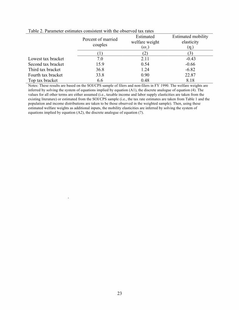
23

Table 2. Parameter estimates consistent with the observed tax rates Percent of married

couples

Estimated welfare weight

€

(ω i)

Estimated mobility elasticity

€

(ηi) (1) (2) (3) Lowest tax bracket 7.0 2.11 -0.43 Second tax bracket 15.9 0.54 -0.66 Third tax bracket 36.8 1.24 -6.82 Fourth tax bracket 33.8 0.90 22.87 Top tax bracket 6.6 0.48 8.18 Notes: These results are based on the SOI/CPS sample of filers and non-filers in FY 1990. The welfare weights are inferred by solving the system of equations implied by equation (A1), the discrete analogue of equation (4). The values for all other terms are either assumed (i.e., taxable income and labor supply elasticities are taken from the existing literature) or estimated from the SOI/CPS sample (i.e., the tax rate estimates are taken from Table 1 and the population and income distributions are taken to be those observed in the weighted sample). Then, using these estimated welfare weights as additional inputs, the mobility elasticities are inferred by solving the system of equations implied by equation (A2), the discrete analogue of equation (7).