Incentives to Improve Teaching—Lessons from Latin America
456
Incentives to Improve Teaching Lessons from Latin America EMILIANA VEGAS, Editor DIRECTIONS IN DEVELOPMENT DIRECTIONS IN DEVELOPMENT Public Disclosure Authorized Public Disclosure Authorized Public Disclosure Authorized ublic Disclosure Authorized
Transcript of Incentives to Improve Teaching—Lessons from Latin America

Incentives toImprove TeachingLessons from Latin America
EMILIANA VEGAS, Editor
D I R E C T I O N S I N D E V E L O P M E N TD I R E C T I O N S I N D E V E L O P M E N T
Pub
lic D
iscl
osur
e A
utho
rized
Pub
lic D
iscl
osur
e A
utho
rized
Pub
lic D
iscl
osur
e A
utho
rized
Pub
lic D
iscl
osur
e A
utho
rized


Incentives toImprove TeachingLessons from Latin America
Emiliana Vegas Editor
THE WORLD BANKWashington, D.C.

© 2005 The International Bank for Reconstruction and Development / The World Bank1818 H Street, NWWashington, DC 20433Telephone 202-473-1000Internet www.worldbank.orgE-mail [email protected]
All rights reserved.
1 2 3 4 08 07 06 05
The findings, interpretations, and conclusions expressed herein are those of theauthor(s) and do not necessarily reflect the views of the Board of Executive Direc-tors of the World Bank or the governments they represent.
The World Bank does not guarantee the accuracy of the data included in thiswork. The boundaries, colors, denominations, and other information shown onany map in this work do not imply any judgment on the part of the World Bankconcerning the legal status of any territory or the endorsement or acceptance ofsuch boundaries.
Rights and PermissionsThe material in this work is copyrighted. Copying and/or transmitting portions
or all of this work without permission may be a violation of applicable law. TheWorld Bank encourages dissemination of its work and will normally grant per-mission promptly.
For permission to photocopy or reprint any part of this work, please send arequest with complete information to the Copyright Clearance Center, Inc., 222Rosewood Drive, Danvers, MA 01923, USA, telephone 978-750-8400, fax 978-750-4470, www.copyright.com.
All other queries on rights and licenses, including subsidiary rights, should beaddressed to the Office of the Publisher, World Bank, 1818 H Street NW, Wash-ington, DC 20433, USA, fax 202-522-2422, e-mail [email protected].
Cover photo: Curt Carnemark/World Bank, 1994ISBN 0-8213-6215-1 e-ISBN 0-8213-6216-XEAN 978-0-8213-6215-0 DOI 10.1596/978-0-8213-6215-0
Library of Congress Cataloging-in-Publication Data
Incentives to improve teaching : lessons from Latin America / Emiliana Vegas, editor.p. cm. — (Directions in development)
Includes bibliographical references and index.ISBN 0-8213-6215-11. Teachers—Salaries, etc.—Latin America—Cross-cultural studies. 2. Rewards and
punishments in education—Latin America—Cross-cultural studies. 3. School improvementprograms—Latin America—Cross-cultural studies. I. Vegas, Emiliana II. World Bank. III.Directions in development (Washington, D.C.)
LB2844.L29I53 2005331.2'813711'0098—dc22
2005047500

Contents
Preface
Acknowledgments
1 Improving Teaching and Learning through Effective Incentives
Lessons from Education Reforms in Latin America
Emiliana Vegas and Ilana Umansky
IntroductionWhy and How Do Incentives Matter?Incentives as a Broad and Complex ConceptTeacher Effectiveness and Student PerformanceA Wide System Affecting Teaching and LearningEducation Reforms, Teaching Quality, and Student LearningReview of ChaptersImproving Teaching Quality and Student Learning
through Incentives An Agenda for Further Research on Teacher Incentives
2 A Literature Review of Teacher Quality and IncentivesTheory and Evidence
Ilana Umansky
IntroductionPrincipal–Agent Theory: Description and CritiquesTeacher Quality and Its DeterminantsCurrent Educational Investment and Policies and
Their Embedded IncentivesMerit PaySchool OrganizationPolitical Economy of ReformSummary and Conclusions
ii i
xiii
xv
1
1 3 4 4 6 6 7
1315
21
212225
2835434749
3 Are Teachers Well Paid in Latin America and the Caribbean?
Relative Wage and Structure of Returns of Teachers
Werner Hernani-Limarino
IntroductionHow Can We Determine If Teachers Are Well Paid?Are Teachers Well Paid?Conclusions
4 Teachers’ Salary Structure and Incentives in Chile
Alejandra Mizala and Pilar Romaguera
IntroductionWho Are Chile’s Teachers?How Teachers’ Salaries Are DeterminedChanges in Teachers’ SalariesEffect of Salary Trends on Individuals Applying to Study
EducationAnalysis of Relative Teacher PayIncentives Embedded within Teachers’ Salary StructureEffect of the SNED on Schools’ Academic Achievement:
A Preliminary EvaluationEvaluating Performance and Incentives: Teachers’ and
Principals’ PerceptionsConclusions
5 Educational Finance Equalization, Spending, Teacher Quality, and Student Outcomes
The Case of Brazil’s FUNDEF
Nora Gordon and Emiliana Vegas
IntroductionBackground on Brazil’s Education System and FUNDEFDataEmpirical StrategyFindingsConclusions and Policy Implications
6 Arbitrary Variation in Teacher SalariesAn Analysis of Teacher Pay in Bolivia
Miguel Urquiola and Emiliana Vegas
Introduction
IV CONTENTS
63
63 65 74 96
103
103 104 105 107
110 115 127
131
141 144
151
151 154 158 168 173 182
187
187

DataTeacher Pay in BoliviaWhat Does the Pay Scale Reward?The Flow of Teachers through the Salary StructureArbitrary Variation in Teacher SalariesConclusions
7 Teacher and Principal Incentives in Mexico
Patrick J. McEwan and Lucrecia Santibáñez
IntroductionThe Carrera Magisterial ProgramDataAllocation of PromotionsEmpirical StrategyResults for TeachersResults for PrincipalsConclusions
8 Decentralization of Education, Teacher Behavior, and Outcomes
The Case of El Salvador’s EDUCO Program
Yasuyuki Sawada and Andrew B. Ragatz
IntroductionThe Case of El Salvador’s EDUCO ProgramEmpirical Analysis of the EDUCO ProgramConclusions
9 Teacher Effort and Schooling Outcomes in Rural Honduras
Emanuela di Gropello and Jeffery H. Marshall
IntroductionAnalytical FrameworkResultsConclusions
10 Teacher Incentives and Student Achievement in Nicaraguan Autonomous Schools
Caroline E. Parker
IntroductionNicaraguan Context
VCONTENTS
189189192197200210
213
213216217222228235245249
255
255257262300
307
307308314353
359
359359

Nicaraguan AutonomyMethodsResultsConclusions
11 Political Economy, Incentives, and Teachers’ UnionsCase Studies in Chile and Peru
Luis Crouch
BackgroundCase Study of Chile: Reforms Designed and Implemented,
Effect Yet to Be SeenCase Study of Peru: Incentives Reforms Underdesigned,
UnimplementedToward a Conclusion: Unions, Incentives, and Educational
Progress in Latin America
Figures1.1 Many Types of Teacher Incentives Exist3.1 Unconditional Log Hourly Wage and Monthly Earnings
Differential3.2 Hours Worked Per Week3.3 Unconditional Log Wage Differential between Teachers and
Different Samples of Nonteachers3.4 Conditional Log Wage Differential between Teachers and
Different Samples of Nonteachers: Estimated Coefficient for the Teachers’ Dummy
3.5 Productivity Log Wage Differential between Teachers andDifferent Samples of Nonteachers: Estimated Endowment Effect from the Oaxaca Decomposition
3.6 Conditional Log Wage Differential between Teachers and Different Samples of Nonteachers: Estimated Price Effect from the Oaxaca Decomposition
3.7 Contribution of the Difference in the Return to Schooling to the Conditional Log Wage Differential
3.8 Contribution of the Difference in the Returns to PotentialExperience to the Conditional Log Wage Differential
3.9 Contribution of the Difference in Women’s Wage Premiumsto the Conditional Log Wage Differential
3.10 Contribution of the Difference in Rural Residence Wage Premium to the Conditional Log Wage Differential
3.11 Contribution of the Difference in Initial Wage to the Conditional Log Wage Differential
VI CONTENTS
360 367 378 383
389
389
390
405
417
5
66 67
78
80
83
85
88
89
91
92
93

3.12 Conditional Log Wage Differential between Teachers andNonteachers by Quantile of the Conditional Wage Distribution
4.1a Hourly Income Distribution of Teachers and All Nonteachers, 1998
4.1b Hourly Income Distribution of Teachers and Nonteachers with 13 or More Years of Schooling, 1998
4.1c Hourly Income Distribution of Teachers and Nonteachers with 17 or More Years of Schooling, 1998
4.2a Hourly Income Distribution of Teachers and All Nonteachers, 2000
4.2b Hourly Income Distribution of Teachers and Nonteachers with 13 or More Years of Schooling, 2000
4.2c Hourly Income Distribution of Teachers and Nonteachers with 17 or More Years of Schooling, 2000
4.3a Salary Differentials between Female Teachers and Nonteachers, 1998
4.3b Salary Differentials between Male Teachers andNonteachers, 1998
4.4 Allowances and Monetary Incentives for Teachers,2002/03
4.5 Responses of Principals: “I Agree or Strongly Agreewith MINEDUC Regularly Evaluating SchoolsReceiving State Subsidies”
4.6 Responses of Principals: “I Agree or Strongly Agree ThatMINEDUC Should Provide Resources for RegularlyRewarding the Best Performing Schools”
4.7 Responses of Principals: “It Is ‘Very Useful,’ ‘SomewhatUseful,’ ‘Useful’ to Principal’s Work That There Is aMonetary Award to Teachers, Associated with SchoolPerformance, Financed and Designed to MINEDUCStandards”
5.1 Evolution of Enrollment in Basic Education, by Leveland Region, 1996–2002: EF1
5.2 Evolution of Enrollment in Basic Education, by Leveland Region, 1996–2002: EF2
5.3 Gross Primary Enrollment Rates by Region, 1994–20005.4 Net Primary Enrollment Rates by Region, 1994–20005.5 Percentage of Qualified Teachers by Region, 1996–20026.1 Salary Progression for Urban Teachers of All Training Levels6.2 Distributions of Salaries for Urban and Rural Teachers6.3 GIS Data for Santa Cruz Schools7.1 Fitted Values of Promotion on Final Points, by Year,
for Teachers
VIICONTENTS
95
118
118
119
119
120
120
128
128
130
143
143
144
159
160 160 161 162 194 203 209
225

7.2 Fitted Values of Promotion on Final Points, by Year,for Principals
7.3 Stylized Portrayal of Empirical Strategy7.4 Fitted Values of Classroom Test Scores on Initial Points,
by Bandwidth for Teachers7.5 Kernel Densities of Test Score for Teachers7.6 Fitted Values of Classroom Test Scores on Initial Points,
by Bandwidth and State, for Teachers7.7 Test Scores and Pupil–Teacher Ratios in Year 10 for Teachers7.8 Fitted Values of Classroom Test Scores on Initial Points,
by Bandwidth for Principals7.9 Fitted Values of Classroom Test Scores on Initial Points,
by Bandwidth and State8.1 Comparison of EDUCO and Traditional Governance
Structures8.2 OLS Estimated Coefficients on the EDUCO Variable for
Major Influence Level of Key Administrative Processes8.3 Estimated Coefficients for EDUCO Perceived Amount of
Influence Compared with Traditional Schools9.1 Model of Effective Community School, With (Some)
Testable Hypotheses
Tables3.1 Household Surveys3.2 Occupational Codes Included in the Definition of Teachers3.3 Size of Teachers’ Sample3.4 Alternative Definitions of Nonteachers3.5. Unconditional Log Wage Differential between Teachers and
Different Samples of Nonteachers: ln(GTN + 1)3.6 Conditional Log Wage Differential between Teachers and
Different Samples of Nonteachers: Estimated Price Effectfrom the Oaxaca Decomposition:E[ln(wT)\X] – E[ln(wN)\X]
3.7 Conditional Log Wage Differential between Teachers andDifferent Samples of Nonteachers: Estimated Price Effectfrom the Oaxaca Decomposition: ln(DTN + 1)
3.8 Productivity Log Wage Differential between Teachers and Different Samples of Nonteachers: Estimated Endowment Effect from the Oaxaca Decomposition: ln(QTN + 1)
3.9 Conditional Log Wage Differential between Teachers andSample 1 of Nonteachers by Quantile
4.1 Monthly Real Salaries of Full-Time (44 Hours) Teachers4.2 Comparison of Teachers’ Salaries with the Average Wage
and Professionals’ Salaries
VIII CONTENTS
227232
235239
241245
246
248
259
274
275
310
73757777
79
81
84
86
96 107
108

4.3 Comparison of Teachers’ Starting Salary with theNational Minimum Wage
4.4 International Comparisons of Teachers’ Salaries, 20014.5 Total Expenditures of the Ministry of Education, 1990–20014.6 Average Score for Admission to Teaching Programs4.7 Means and Standard Deviations of Selected Variables
in a Comparison of Teachers and Nonteachers, 1998and 2000
4.8 Determinants of Labor Income, Teachers Comparedwith Nonteachers, 1998
4.9 Factors Determining Labor Income, Teachers Comparedwith Nonteachers, 2000
4.10 Breakdown of the Wage of an Average Municipal SectorTeacher, 2003
4.11 SNED: Beneficiaries and Resources4.12 Trends in SNED Award Amounts4.13 SNED’s Effect on Effectiveness4.14 SNED Relationship to Effectiveness5.1 Mean Per Pupil Spending and Enrollment Rates by Region5.2 Share of Teachers in Grades 1–4 with Credentials Higher
Than Primary Education, 19965.3 Sources and Distribution Mechanisms of FUNDEF Funds,
by Government Level5.4 Number of Teachers by Level, Region, and Year5.5 Mean Pupil-to-Teacher Ratio by Level, Region, and Year5.6 Age-by-Grade Distortion by Region, Level, and Year5.7 Annual FUNDEF Per Pupil Allocations by Region, State,
and Year5.8 Mean Per Pupil Spending, by Region and Year5.9 Mean Net FUNDEF Per Pupil Allocation and Mean Per
Pupil Expenditures, 1998–20025.10 Means, Standard Deviations, and Gini Coefficients for
SAEB Language Scores in 1995, 20015.11 Means, Standard Deviations, and Gini Coefficients for
SAEB Mathematics Scores in 1995, 20015.12 Stage 1: Effect of Mandated Educational Spending on
Actual Educational Spending5.13 Stage 1: Effect of Mandated Educational Spending on
Actual Per Pupil Educational Spending, by Geographic Region
5.14 Stage 1: With Year-Specific Predictors5.15 State-Level Effects of Spending on Enrollment, by Level5.16 Effects of Educational Spending Per Pupil on Class Size,
by Level
IXCONTENTS
109 111113115
117
122
123
130132133139140155
156
157161162163
165166
167
167
168
173
174174175
177

5.17 Effects of Educational Spending Per Pupil on Share ofTeachers with Credentials Higher Than PrimaryEducation, by Level
5.18 Effects of Educational Spending Per Pupil on Age-by-Grade Distortion, by Level
5.19 Effects of Education Inputs on Age-by-Grade Distortion,by Level
5.20 Estimated Effect of Changes in State-Level Mean Per Pupil Spending on Mathematics Student Achievement by Percentile
5.21 Estimated Effect of Changes in State-Level Inequality in PerPupil Spending on Mathematics Student Achievementby Percentile
6.1 Base Salaries by Geographic Region and Training Status6.2 Seniority-Based Pay Increases: Escalafón6.3 Salary Structure6.4 A Hypothetical Decomposition of the Teacher Wage Bill6.5 A Decomposition of the Teacher Wage Bill6.6 Distribution of Teachers by Geographic Region
and Training Status6.7 Distribution of Teachers by Training and Experience6.8 Types of Schools in the Three Largest Cities6.9 Descriptive Statistics on Teachers6.10 Hours Worked and the Probability of Holding a Second
Teaching Job6.11 Student Characteristics in Urban and Rural Schools6.12 Hours Worked by Teachers and Probability of Holding a
Second Job7.1 Evaluation Scheme for Carrera Magisterial7.2 Teacher Promotions in Carrera Magisterial7.3 Principal Promotions in Carrera Magisterial7.4 Descriptive Statistics for Teachers7.5 Descriptive Statistics for Principals7.6 Determinants of Teacher Promotion, by State7.7 Determinants of Principal Promotion, by State7.8 Teachers’ Initial Points and Classroom Test Scores7.9 Teachers’ Initial Points and Classroom Test Scores,
within Narrow Bands7.10 Teachers’ Initial Scores and Classroom Test Scores:
Difference-in-Differences7.11 Principals’ Initial Points and School Performance Scores7.12 Principals’ Initial Scores and Classroom Test Scores:
Difference-in-Differences8.1 Means and Standard Deviations of Municipality-Level
Socioeconomic Variables
X CONTENTS
178
179
180
181
181 190 191 192 195 196
199 199 201 202
204 206
207 217 219 220 221 222 226 229 237
238
242 247
249
261

8.2 Means and Standard Deviations of Child and HouseholdVariables, by School Type
8.3 Means and Standard Deviations of School, Teacher,Classroom, and Community Variables, by School Type
8.4 The Format of Questions on the Administrative Process8.5 Means and Standard Deviations of Decentralization and
Perceived Influence Variables8.6 Means and Standard Deviations for Control Variables
Used in Administrative Process Regressions8.7 Level of Decentralization: Comparison of OLS Results
to Propensity Score and Treatment Effects Results8.8 Influence Level by Group: Comparison of OLS Results
to Propensity Score and Treatment Effects Results8.9 Means and Standard Deviations of Control Variables Used
in Teacher Behavior Regressions8.10 Means and Standard Deviations of Control Variables Used
in Teacher Behavior Regressions8.11 Comparison of OLS Results to Treatment Effects and
Propensity Score Matching Results8.12 Means and Standard Deviations of Student Achievement
Test Scores8.13 Estimated EDUCO Effects on Mathematics Scores8.14 Estimated EDUCO Effects on Spanish Scores8.15 Estimated Effects on Days of Absence9.1 Sample Overview: Number of Students and Schools
(in Parentheses), by Department9.2 Comparisons of Student and Family Characteristics among
PROHECO and Control Samples9.3 Comparisons of School Characteristics between PROHECO
and Control Samples9.4 Comparisons of Teachers’ Characteristics9.5 Comparisons of Teacher Work Hours and Absences9.6 Comparisons of Teacher Salaries and Payment “Issues”9.7 Teacher Earnings Equations9.8 Comparisons of Teaching Strategies9.9 Comparisons of Teacher Planning Strategies, Part 19.10 Comparisons of Teaching Strategies, Part 29.11 Comparisons of Teacher Attitudes, Part 19.12 Comparisons of Teacher Attitudes, Part 29.13 Comparisons of School Environments According to
Students9.14 School Characteristics According to Directors9.15 PROHECO Parameter in Regressions of Teacher and
School Effort on Various Groupings of Variables9.16 Summary of Test Scores
XICONTENTS
262
263 265
269
271
278
279
287
290
292
297 298 299 300
316
317
318 319 320 322 323 325 326 327 328 329
330 332
334 336

9.17 OLS Estimates of Determinants of Spanish Achievement,2002 and 2003
9.18 OLS Estimates of Determinants of MathematicsAchievement, 2002 and 2003
9.19 OLS Estimates of Determinants of Science Achievement,2002 and 2003
9.20 Breakdown of PROHECO and Control SchoolAchievement Differences, 2003
9.21 First-Stage Equations: Binary Probit Estimates ofPROHECO Participation, 2002 and 2003
9.22 Comparison of PROHECO Achievement Effect UsingPredicted and Actual Measure of PROHECOParticipation, 2002 and 2003
9.23 Ordered Probit Estimates of Student-Reported Absences,2002 and 2003
9.24 OLS Estimates of Determinants of School Average Repetitionand Dropout Rates, 2002 and 2003
10.1 Control Variables: Third-Grade Mean Values, by School Type10.2 Years of School Autonomy, Third Grade10.3 Third-Grade Descriptive Statistics for Incentive Variables10.4 Third-Grade Descriptive Statistics for Infrastructure and
Material Resources, by School Type10.5 Third-Grade Descriptive Statistics for Professional
Development, by School Type10.6 Third-Grade Achievement Scores, by School T10.7 Third-Grade Spanish and Math Scores, by Years of Autonomy 10.8 Control Variables: Sixth-Grade Mean Values, by School Type10.9 Years of School Autonomy, Sixth Grade10.10 Sixth-Grade Descriptive Statistics for Incentive Variables10.11 Sixth-Grade Descriptive Statistics for Infrastructure/
Material Resources, by School Type10.12 Sixth-Grade Descriptive Statistics for Professional
Development, by School Type10.13 Sixth-Grade Achievement Scores, by School Type10.14 Spanish and Math Scores, by Years of Autonomy10.15 Third-Grade Spanish Achievement10.16 Third-Grade Mathematics Achievement10.17 Third-Grade Mean Difference in Scores between
Autonomous and Centralized Schools, by Process10.18 Sixth-Grade Spanish Achievement10.19 Sixth-Grade Math Achievement10.20 Sixth-Grade Mean Difference in Scores between
Autonomous and Centralized Schools, by Process11.1 Relationship of Incentives to Attributability of Results11.2 Promotion Criteria According to Ley del Profesorado
XII CONTENTS
337
339
341
346
348
349
352
354371372372
373
374ype 374
374 375 376 376
377
377 378 378 379 380
380 381 382
382 403 408

Preface
This book is about one of the most pressing challenges in improving edu-cation quality in Latin America: designing and implementing effectiveincentives for enhancing teaching practice as a means for raising studentlearning outcomes. The various evaluations presented in the volumetackle this issue using the best available data and latest methodologicalapproaches to provide insights into why and how education reforms canaffect who chooses to enter and remain in the teaching profession and howeffective are teachers in fostering student learning.
By providing well-researched evidence on diverse education reformsaffecting teacher incentives in the region, the book makes an importantcontribution to the literature on teacher incentives in general and, espe-cially, to the education literature in Latin America. Perhaps more impor-tant, the lessons on teacher incentive reforms from this research can beuseful to policy makers in Latin America and in the rest of the world.
The research in this book provides evidence that teachers respond toincentives, and that these vary in nature: some incentives affect whodecides to enter and remain in the teaching profession, while other incen-tives affect the work teachers do in classrooms. How well teachers are paidrelative to similar workers in other professions affects teaching quality.Additionally, changes in the structure of pay—in which teachers arerewarded for doing specific things, such as mentoring new teachers orhaving students perform better in tests, can lead to higher student learn-ing. But pay incentives appear to be more powerful when teachers can losetheir jobs as a result of poor performance. As in most policy reforms, in thecase of teacher incentive reforms, too, the devil is in the details. The casesin this volume show that clarity in the behaviors that are being motivated,as well as real differentiation in the rewards to teachers who adopt thedesired behaviors and those who do not, can have a big impact on theeffectiveness of teacher incentive reforms.
Changes in other aspects of teacher contracts can also have a greatimpact on teaching quality and student learning. Education reforms, eventhose not specifically designed to affect teachers, can influence—andsometimes have even greater effects than changes in compensation—thecharacteristics of those who choose to enter and remain in teaching and,
xii i

importantly, their work in classrooms. For example, school-based man-agement reforms that devolve decision-making authority to the schoolwere found to have had an important impact on teacher performance andstudent learning.
Although Latin American countries are continuously reforming theireducation systems, it is rare to find examples in which findings fromsound evaluations inform reform design. This study is an important con-tribution to fill this void.
Guillermo Perry Ariel FiszbeinChief Economist Lead EconomistLatin America and the Caribbean Human Development
Region DepartmentThe World Bank Latin America and the Caribbean
RegionThe World Bank
XIV PREFACE

Acknowledgments
This publication is possible thanks to the collaboration and support frommany colleagues and friends. I am indebted to Beth King, who first en-visioned this project with me, and with whom I co-authored the initialproposals to obtain funding for this research. For their constant supportthroughout the various stages to produce this book, I am grateful to ArielFiszbein, Marito Garcia, Guillermo Perry, Luis Serven, and Eduardo VelezBustillo.
Special thanks go to the authors of each of the chapters, including: LuisCrouch, Emanuela Di Gropello, Nora Gordon, Werner Hernani-Limarino,Jeffery Marshall, Patrick McEwan, Alejandra Mizala, Carrie Parker, AndyRagatz, Pilar Romaguera, Lucrecia Santibáñez, Yasuyuki Sawada, IlanaUmansky, and Miguel Urquiola.
Many individuals contributed to improve the research, and its presen-tation, with very helpful comments and suggestions. Among them:Charles Abelmann, Jishnu Das, Andrea Guedes, Gustavo Ioschpe, PeterMoock, Richard Murnane, Vicente Paqueo, Harry Patrinos, Jeff Puryear,Alberto Rodríguez, Halsey Rogers, Jaime Saavedra, Carolina SánchezPáramo, Luis Serven, Sergei Soares, and Kristian Thorn. As usual, only theauthors and the editor are responsible for any remaining errors.
xv


1Improving Teaching
and Learning through Effective Incentives
Lessons from Education Reforms in Latin America
Emiliana Vegas and Ilana UmanskyThe World Bank
As a region, Latin America faces tremendous challenges, particularly thoseof development, poverty, and inequality. Education is widely recognized asone of the most critical means of defeating those challenges. Democratizingeducation—by improving both its coverage and its quality—is critical toovercoming the social and economic inequality that plagues Latin Amer-ica. Ensuring that all children have the opportunity to learn critical skills atthe primary and secondary level is paramount to overcoming skill barriersthat perpetuate underdevelopment and poverty.
Although most people recognize the importance of improving the qual-ity of education systems for reducing poverty and inequality and forincreasing economic development, how to do so is less clear. A growingbody of evidence supports the intuitive notion that teachers play a key rolein what, how, and how much students learn (see, for example, Hanushekand others 2005; Park and Hannum 2001; Rivkin, Hanushek, and Kain1998; Rockoff 2004; Sanders and Rivers 1996; Wright, Horn, and Sanders1997). Attracting qualified individuals into the teaching profession, retain-ing those qualified teachers, providing them with the necessary skills andknowledge, and motivating them to work hard and to do the best job theycan is arguably the key education challenge.
This book, Incentives to Improve Teaching—Lessons from Latin America,focuses on the effect of education reforms that alter teacher incentives toachieve teaching quality and to enhance student learning. The goals of ourbook are, first, to broaden and deepen our conception of how educationreforms affect teachers in Latin America and, second, to shed light on how
1

reforms can be designed and implemented to maximize their beneficialeffects on teaching and learning. We hope to demonstrate which teacherincentive reforms have been most successful at improving teaching andlearning in the region, as well as to shed some light on the importance ofhow reforms are negotiated in the larger society, particularly by lookingat the important role of teachers’ unions.
The reforms explored in this volume represent efforts by several coun-tries in the region to increase teachers’ accountability and to introduce incen-tives to motivate teachers so they raise student learning. Some countries—such as Bolivia, Chile, and Mexico—have established salary differentials,thereby rewarding teachers for working in rural areas, or have introducedsalary structures that reward teachers for improved performance andstudent learning. Brazil changed the resources available for educationgenerally and for teacher salaries more specifically, as well as the mecha-nisms by which the resources are made available to municipality and state-level education systems. El Salvador, Honduras, and Nicaragua devolvedtheir authority to communities, thus granting professional autonomy toschools and teachers in the belief that the increased accountability wouldlead to higher teaching quality and student outcomes.
Policy options to improve teaching quality can be grouped into threemain clusters: (a) policies to improve teacher preparation and professionaldevelopment, (b) policies that affect who becomes a teacher and how longhe or she remains in the field, and (c) policies that affect the work thatteachers do in the classroom. This volume focuses entirely on the secondand third options, both of which can be understood as policies that createincentives to positively affect teachers and their work.
Teacher training and professional development have received atten-tion in the past from educators, policymakers, researchers, and the inter-national donor community.1 In contrast, the literature on policies thatgenerate teacher incentives in Latin America is not very extensive.Although previous studies have addressed questions related to teachingquality and incentives in Latin America,2 ours is the first study that weare aware of in which researchers sought to learn about the effect of vari-ous policy reforms affecting teachers on teaching quality and studentachievement in multiple Latin American countries.
Because teacher incentive reforms are frequently politically contestedand are difficult to implement, many countries have shied away fromchanging their prevailing structures of teacher incentives. The selection
2 INCENTIVES TO IMPROVE TEACHING
1. For a review of the literature and assessment of current teacher preparation systems inLatin America, see Villegas-Reimers (1998); for a review of recent trends and innovations inteacher preparation programs in the region, see Navarro and Verdisco (2000).
2. See, for example, Navarro (2002) for various case studies that describe many aspectsof teacher contracts and teacher characteristics in several Latin American countries.
of case studies in our volume was largely determined by the presence ofa reform affecting the teaching profession. Our methodological approachentails using existing data and econometric techniques to shed light on theeffect of such reforms on teaching quality and incentives. Our analyseshave been limited by the quality of the data available, and we have usedalternative econometric and statistical techniques in an attempt to overcomesome of the shortcomings of existing data.
Why and How Do Incentives Matter?
A substantial amount of the literature on incentives in firms has empha-sized that the interests of workers (teachers) and their employers (princi-pals, education authorities, or school boards) are often not aligned. Forexample, although school administrators and education authorities maybe interested in attracting more students to their schools, teachers maywant to keep some difficult-to-teach students out of their classrooms.Compensation contracts may be designed to include incentives that willlead workers (teachers) to operate in the interest of the firms (schools).3
In the example above, school administrators could devise incentives(such as extra pay or promotion possibilities) so that teachers will keep allstudents in their classrooms.
Evidence suggests that changes in teacher incentive structures can affectwho chooses to enter and remain in the teaching profession, as well as thoseteachers’ daily work in the classroom. For example, in the United States,where there is growing concern about the declining quality of teachers,recent research shows that the increase in labor market opportunities forwomen led to a decrease in the pool of qualified applicants for teachingpositions.4 At the same time, research suggests that teacher salary scales inthe United States are so compressed that the best teachers are likely to leavethe profession for higher-salaried jobs in other occupations.5
In less industrial countries, recent research indicates that teachersrespond to incentives. For example, an evaluation of a randomized teacherincentives program in Kenya found that teachers increased their effort toraise student test scores by offering more test-preparation sessions(Glewwe, Ilias, and Kremer 2003). In this program, a financial bonus was
3IMPROVING TEACHING AND LEARNING
3. For a review of the literature about providing incentives in firms, see Prendergast(1999).
4. Corcoran, Evans, and Schwab (2004) and Hoxby and Leigh (2004) present evidence thatthe quality of teachers in the United States has declined over time because of changing labormarket opportunities.
5. Hoxby and Leigh (2004) present evidence that the decline in teacher quality in theUnited States is a result not only of increased opportunities for women outside of teaching,but also of the highly compressed structure that deals with teaching wages.

offered to teachers whose students achieved higher scores on a standard-ized examination. Although student test scores of teachers who were can-didates for the bonus did increase in the year it was applied, the learninggains disappeared once the application of the financial bonus ended andteachers had no longer a chance of earning additional pay. More promising,a recent evaluation of a performance-based pay bonus for teachers in Israelconcluded that the incentive led to increases in student achievement, pri-marily through changes in teaching methods, after-school teaching, andteachers’ increased responsiveness to students’ needs (Lavy 2004).
Because teachers respond to incentives, education policymakers canimprove the quality of teaching and learning by designing effective incen-tives that will attract, retain, and motivate highly qualified teachers. Buthow teacher incentives are designed—and implemented—also matters.In various cases, teachers have been found to respond adversely to incen-tives by, for example, reducing collaboration among teachers themselves,excluding low-performing students from classes, cheating on or manipu-lating the indicator on which rewards are based, decreasing the academicrigor of classes, or “teaching to the test” to the detriment of other subjectsand skills (see Cullen and Reback 2002; Figlio and Getzler 2002; Figlioand Winicki 2002; Jacob and Levitt 2003; Murnane and Cohen 1986).
Incentives as a Broad and Complex Concept6
Many people think of teacher incentives exclusively as salary differen-tials and other monetary benefits. Indeed, differences in pay can act as anincentive to attract and retain qualified teachers or, conversely, can dis-courage qualified applicants and talented practitioners who are alreadyin the profession. But many other kinds of incentives exist, both mone-tary and nonmonetary, including—among others—adequate school infra-structure and educational materials, the internal motivation to improvechildren’s lives, the opportunity to grow professionally, pensions andother nonsalary benefits, and job stability. Figure 1.1 displays many typesof incentives that may exist for attracting highly qualified teachers andfor motivating them to be effective in their jobs.
Teacher Effectiveness and Student Performance
Who is a good teacher? What makes a good teacher? Everyone who hasbeen through school can remember a great teacher. People usually providea variety of reasons for what makes that teacher great—from being “loving
4 INCENTIVES TO IMPROVE TEACHING
6. We are grateful to Jeff Puryear, whose comments at the conference titled, “Learning toTeach in the Knowledge Society,” which was held in Seville, Spain, in June 2004, greatlyinformed this section.

and caring,” “knowledgeable,” or a “good communicator,” to being“tough” and “pushing me to work hard and expand my horizons.” Thesecomplex behaviors are not easily measured. In fact, measuring the factorsthat effective teachers have—or that ineffective teachers do not have—has proved imprecise, technically difficult, and expensive. This measure-ment problem creates one of the challenges for designing effective teacherincentives.
Ultimately, what society should care about is whether teachers are gen-erating learning within their students. In other words, although having theteachers show affection for the student and command knowledge of thesubject they are teaching are behaviors that are likely to stimulate studentsto learn, not all teachers who are affectionate or knowledgeable are alsoeffective teachers.
In our study, we use a specific definition of teachers’ effectiveness. Weconsider a teacher to be effective when there is evidence that his or herstudents have acquired adequate knowledge and skills. To measure theeffectiveness of teachers, we rely primarily on available indicators of studentlearning from national assessments of subject-matter (usually languageand mathematics) knowledge. Because student learning takes multipleforms and is difficult to measure, and because tests are an imperfect
5IMPROVING TEACHING AND LEARNING
Intrinsicmotivation
Salarydifferentials
Mastery
Job stability
Recognitionand prestige
Respondingto clients
Pensions and
benefits
Professionalgrowth
Adequate infrastructure andteaching materials
Qualified,motivated,
effectiveteachers
Figure 1.1 Many Types of Teacher Incentives Exist

measure of learning, we recognize that test scores are an incomplete andimperfect proxy for teaching quality.7 However, given the absence of a bet-ter understanding of what factors make a good teacher and given thepaucity of systematic and comparable data on student learning, nationalassessments are our best option for shedding light on the quality of teach-ing and learning.
A Wide System Affecting Teaching and Learning
Although teacher incentive reforms are a promising option to improveteaching quality and student learning, they do not operate alone butinstead are part of a broader system that affects teaching and learning. Asa result, reforms to teacher incentives may be more effective in raisingstudent learning when other parts of the broader system affecting teachingand learning are in place. For example, tying salary increases to teacherperformance may be effective only in raising student achievement whenteachers have clarity about what knowledge and pedagogical skills areneeded to improve student learning. Similarly, the benefits of increasedteacher accountability reforms are possible only when teachers know towhom they are accountable and when those individuals, in turn, haveauthority to reward and sanction teachers on the basis of their perfor-mance. In short, effective incentives are a necessary, but not sufficient, con-dition for ensuring teaching quality and student achievement.
Education Reforms, Teaching Quality, and Student Learning
Just as there are many types of teacher incentives, various educationreforms may affect teachers even if not originally planned as teacher incen-tive reforms. Policy changes in the level or structure of compensation, aswell as changes in teachers’ professional autonomy, can significantly affectthe teaching profession. The chapters included in our volume approachthe question of the effect of teacher incentive reforms on teaching qualityand on student learning from various angles. Each chapter explores one orseveral aspects of a teacher incentive reform in Latin America andattempts to identify its effect on teaching quality and student learning.
Conducting impact evaluations of education programs is challenginggiven the impossibility of knowing what would have happened to thoseaffected by the program if the program were not present. For example, tounderstand the effect of school attendance on labor market outcomes, we
6 INCENTIVES TO IMPROVE TEACHING
7. Kane and Staiger (2001) and Koretz (2002) provide evidence of the multiple problems inassessing the knowledge of students.
would need to compare two identical individuals at the same time in thesame place, one who attended school and one who did not. Because thiscomparison is impossible in practice, a challenge for the impact evaluationis to construct groups of individuals who can be convincingly compared.In this sense, for evaluation purposes, all participants of education pro-grams should ideally be selected in a randomized fashion. Although, inmany cases, randomized assignment to participate in education pro-grams is not possible, creative ways of analyzing good data about edu-cation programs can yield results that are of comparable quality to thosefrom randomized trials. This approach is the one we took in the chaptersof our volume.
Review of Chapters
The second chapter in our book, by Ilana Umansky, reviews the earlierliterature about teacher incentives. Incentives, in general, and teacherincentives, in particular, have been the subject of much academic andpolicy debate. It is clear that “Incentives do matter, for better or forworse” (Prendergast 1999). That is, incentives have direct implicationson teachers’ characteristics and behavior. However, it is much less clearhow incentives work and under what conditions teachers create thetypes of changes desired. Similarly, it is intuitively clear that teachingquality affects student learning, but it is less evident what qualities makea good teacher or what precise behavior composes good teaching. Chap-ter 2 provides a review of the literature on incentives as they relate toteaching quality, characteristics, and behavior, as well as their relation-ships to student development and learning. It also presents the variousarguments and findings on many of the types of incentives that teachersfrequently face.
Because differences in salary between teachers and nonteachers can havea great effect on who chooses to enter the teaching profession, the thirdchapter, by Werner Hernani-Limarino, addresses the question of how wellteachers are paid relative to comparable workers in other occupations. As inother parts of the world, people in Latin America have a widely held beliefthat teachers are not well paid and that, in general, teachers earn less thanthey would in other professions. Yet, previous research has found that, inmany cases, teachers in Latin America may be paid more than workers withsimilar characteristics in many countries (see Liang 1999, for example). Inhis study of teachers’ salaries in 17 Latin American countries, Hernani-Limarino, however, demonstrates that relative salaries for teachers varywidely across Latin America and depend largely on to whom teachers arecompared and what methods are used to make those comparisons.
He finds that teachers in Argentina, Chile, Colombia, El Salvador,Honduras, Panama, Paraguay, and Peru are, on average, paid more than
7IMPROVING TEACHING AND LEARNING

comparable workers in other occupations. Teachers in Nicaragua earnlower average wages than do workers in other fields. But in Bolivia, Brazil,Costa Rica, the Dominican Republic, Ecuador, Mexico, Uruguay, andVenezuela whether teachers are well paid varies depending on the com-parison group used in the analysis. Hernani-Limarino develops severalcomparison groups but finds that when compared to workers in office,technical, and professional occupations—arguably the most appropriatecomparison group because the workers tend to have similar educationallevels as teachers—teachers do not have a pay advantage in any of thoseeight countries.
Chapter 3 also compares the structures of teachers’ salaries with those ofworkers’ salaries in other occupations. In the 17 Latin American countriesexamined, the teachers’ wage structure is flatter and begins at a higher levelthan the salary structure of nonteachers. Although teachers throughoutthe region receive higher base salaries than do comparable workers in otheroccupations, teachers receive lower returns than do nonteachers when wecompare their improved characteristics, such as higher education or train-ing plus additional years of experience. In practice, then, teachers earn com-paratively higher salaries than they would outside of teaching when theyare at the lower end of the wage distribution (that is, have less educationand experience), while teachers with more education and experience earnthe same or less than they would in other professions.8
Chapter 4, by Alejandra Mizala and Pilar Romaguera, explores theteachers’ salary structure in Chile and its related incentives. In Chile,changes in wage levels were accompanied by changes in the overallnumber, as well as the quality, of applicants to the teaching profession.Teachers experienced a 32 percent decline in real salaries in the 1980s as aresult of government budget reductions. Over this same period, the num-ber of students entering education programs dropped 43 percent. In the1990s, both trends reversed. Between 1990 and 2002, real teachers’ salariesincreased 156 percent, and as a result teachers in Chile are now paid highersalaries than comparable workers in other occupations. At the same time,there was a 39 percent increase in the number of education students, andthe average score for applicants to education programs increased 16 per-cent. This improvement in applicant quality did not take place across alldegree programs, such as engineering, where the average entrance examscore remained more or less constant. Those patterns suggest that changesin salary level can affect individuals’ choices to become a teacher.
8 INCENTIVES TO IMPROVE TEACHING
8. Note that teachers’ pensions and other nonsalary benefits are not dealt with in thisdiscussion. Pensions are, however, widely believed to be quite high when compared withnonteachers’ pensions, to be earned at an earlier age, and to be fiscally secure. High, early,and secure pensions may be a strong incentive for teachers to enter and remain in the field.

In 1996, Chile introduced the SNED (Sistema Nacional de Evaluaciónde Desempeño de los Establecimientos Educacionales, or National Systemof School Performance Assessment), which offers monetary bonuses toschools that show excellent performance in terms of student achievement.Teachers in winning schools receive what has typically amounted to one-half of one month’s salary, or between 5 and 7 percent of a teacher’s annualsalary. Although impact evaluations of the SNED are difficult owing to theabsence of a natural control group, this chapter provides some preliminaryevidence that the incentive has had a cumulative positive effect on studentperformance for those schools facing relatively good chances of winningthe award.
In Chapter 5, Nora Gordon and Emiliana Vegas evaluate the effect thata large reform of educational finance has had in Brazil on educationalspending, teaching quality, and student outcomes. Brazil is a vast countrycharacterized by large inequalities in educational spending and educa-tional outcomes. Those inequalities exist between states and also betweenthe different municipalities within each state. The Fundo de Manutenção eDesenvolvimento do Ensino Fundamental e de Valorização do Magistério(Fund for the Maintenance and Development of Basic Education andTeacher Appreciation, or FUNDEF) reform was implemented in 1998.FUNDEF is a national reform for finance equalization on behalf of primaryeducation in which each state and municipal government in Brazil pools apercentage of educational funds at the state level. Those funds are thenredistributed equally, on a per student basis, to each governmental educa-tion authority (state and municipal). Addressing a long-standing inequalityin educational finance, this reform tends to increase per pupil educationalfunding in municipality-run schools and to decrease per pupil educationalfunding in state-run schools, particularly in the poor northern and north-eastern regions of Brazil.
Among FUNDEF funds, 60 percent is earmarked specifically for teach-ers. Those funds are used to hire new teachers, to train underqualifiedteachers, and to increase teachers’ salaries. Some evidence shows that thegovernments that experienced increases in mandated per pupil spendingactually hired new teachers and decreased class sizes. Gordon and Vegasalso document a sharp rise in teacher educational levels although they findthat this rise was caused less by the FUNDEF reform and more by a leg-islative mandate enacted around the same time.
The FUNDEF reform and the changes it created in educational inputshave, in turn, generated changes in outcomes. More students are nowattending school in the poorer states of Brazil as a result of the reform,specifically in the higher grades of basic education. Additionally, hav-ing teachers who have reached higher educational levels is related tolower levels of overaged students in the classroom. This finding suggeststhat having qualified teachers helps students stay on track in school,
9IMPROVING TEACHING AND LEARNING

repeat less, drop out less, and perhaps also enter first grade on time. Fur-thermore, low-performing students suffer most from inequalities in perpupil spending. This result may indicate that finance equalizationreforms that decrease the spending inequalities may also decrease theperformance gap between high-performing and low-performing studentsand between white and nonwhite students. While the exact mechanismis not clear, giving teachers more competitive salaries, hiring moreteachers, and ensuring that teachers have adequate educational levelsappears to have particularly benefited low-performing and disadvan-taged students in Brazil.
In Chapter 6, Miguel Urquiola and Emiliana Vegas analyze the teachers’salary system in Bolivia and, in particular, the effect of a teacher bonus towork in rural areas. As in many other countries, the rural teacher pay dif-ferential in Bolivia is intended to compensate teachers for the perceivedhardship of living and working in a rural area. As a result of recent urban-ization and demographic growth within cities, some designated ruralschools have been incorporated into urban areas. In those cases, urban andrural teachers work in neighboring schools, sometimes even the sameschool, with indistinguishable groups of students. This chance occurrencecreates a situation in which teaching quality can be compared betweenteachers who are classified as rural (and thus earn higher wages) and thoseclassified as urban.
Urquiola and Vegas found no meaningful differences between the testscores and other educational outcomes of students of urban-classifiedand rural-classified teachers with the same background characteristics.This result suggests that the rural pay differential is not successful atattracting and retaining teachers who are more effective than averageurban teachers. In further support of this finding, rural teachers nationallyare twice as likely as urban teachers to lack full teacher preparation, andthey are also more likely to abandon the profession.
In Chapter 7, Patrick J. McEwan and Lucrecia Santibáñez evaluate theeffect on teaching quality and student outcomes of a teacher pay reform inMexico. Mexico’s Carrera Magisterial Program, which began in 1993, cre-ated a means by which teachers can move up consecutive levels of higherpay on the basis of year-long assessments of a series of factors, includingtheir professional development and education, their years of experience, apeer review, and, most important, their students’ performance. The pur-pose of the reform was to establish incentives for teachers to improve theirqualifications and effectiveness in the classroom and to create a means bywhich teachers could receive promotions without being promoted out ofthe classroom and into administrative positions. The size of the bonusesoffered by Carrera Magisterial are quite substantial, amounting to between24.5 percent of teachers’ base wage for the first promotion and 197 per-cent of base wage for the highest (fifth) promotion.
10 INCENTIVES TO IMPROVE TEACHING

Despite the program’s promise, McEwan and Santibáñez find noapparent effect of the Carrera Magisterial program on student perfor-mance as measured by a standardized exam. Teachers who face greaterincentives because of the reform do not tend to have students with higherachievement. Test scores do not capture the spectrum of ways in whichteaching and learning can improve. The fact (a) that Carrera Magisterialmeasures test scores specifically—thereby creating a strong incentive forteachers to focus on improving scores—and (b) that, nonetheless, testscores have not gone up under the reform suggests that it is unlikely thatany major unmeasured improvements in Mexico’s classrooms resultedfrom the reform.
The next three chapters explore the effect of school-based managementreforms on teaching quality and student outcomes in three Central Amer-ican countries: El Salvador, Honduras, and Nicaragua. Many peoplehypothesize that school-based management generates several incentivesand conditions that can improve teaching quality and teaching. Thoseimprovements include greater accountability to local stakeholders, directcommunication between communities and schools concerning their needsand interests, and more flexible and meritocratic pay and advancementstructures associated with closer-to-the-source evaluation and weakerteachers’ unions.
Chapter 8, by Yasuyuki Sawada and Andrew Ragatz, analyzes theeffect on teaching quality and student learning of the EDUCO program(Programa de Educación con Participación de la Comunidad, or Educationwith Community Participation Program) in El Salvador. They find that thisschool-based management reform has had important effects on manage-ment practices, teacher behavior, and student outcomes although not allof those changes are precisely the ones that were expected or desired. Interms of management practices, Sawada and Ragatz find that although afew important powers have been relocated to the school level, mostnotably the ability to hire and fire teachers, many other decisions appear tocontinue to be made primarily by central authorities. Next, they find thatmost of the local decisionmaking power has been given to parents asopposed to principals. They also find important behavioral differencesbetween EDUCO and control schools, such as fewer school closings, lessteacher absenteeism, more meetings between teachers and parents, andlonger work hours for teachers. The changes, in turn, are related to higherachievement in Spanish in EDUCO schools.
Chapter 9, by Emanuela di Gropello and Jeffery H. Marshall, finds someeffects of the Honduran PROHECO (Proyecto Hondureño de EducaciónComunitaria, or Honduran Community Education Project) that are simi-lar to those found in El Salvador. Like EDUCO, PROHECO is a school-based management reform for rural primary schools. As in reports fromEl Salvador, di Gropello and Marshall present evidence that teacher
11IMPROVING TEACHING AND LEARNING

behavior and characteristics differ between PROHECO and control groupschools. Specifically, they find that PROHECO teachers are less frequentlyabsent because of union participation, although they are more frequentlyabsent as a result of teacher professional development. They also find evi-dence that PROHECO teachers are paid less than are comparison teachersand have fewer years of experience. Similar to El Salvador, evidence showsthat PROHECO teachers teach more hours in an average week than docomparison teachers and that they have smaller classes and assign morehomework. The examples lend credence to the idea of greater efficiencyand teacher effort in decentralized schools. Yet, school-based manage-ment in Honduras has not had much effect in some important areaswhere people expected it would. Namely, little evidence was found thatteachers in community-managed schools differ from their colleagues inconventional schools in terms of their classroom processes, planning,or motivation.
Nevertheless, PROHECO students score higher on math, science, andSpanish exams than do students in similar non-PROHECO schools. Thebenefits of PROHECO are, in part, explained by the qualities and charac-teristics found to be different in PROHECO schools. Specifically, the morehours per week that a teacher works, the higher the student achievementin all three subjects. The frequency of homework is associated with higherachievement in Spanish and math. Finally, smaller classes and fewerschool closings are related to higher student achievement in science.
Chapter 10 covers Caroline E. Parker’s findings from her analysis ofNicaragua’s Autonomía Escolar (School Autonomy) program. Her find-ings from the Nicaragua reform differ considerably from those of the othertwo Central American reforms. To a large degree, those differences mayresult from the major differences in reform design and objectives. UnlikePROHECO and EDUCO, Autonomía Escolar was aimed initially at urbansecondary schools and, in particular, at schools with higher than averageresources. In contrast to their peers in neighboring El Salvador and Hon-duras, parent associations and teachers in Nicaragua’s autonomous schoolsreport little decisionmaking power. A decade after the reform was firstimplemented, very few differences existed between autonomous and non-autonomous schools that were not present in those same schools before thereform. Student background continues to be one of the most important fac-tors explaining differences in student achievement in Nicaragua, and thereis no systematic effect of the reform on student learning. Although third-grade students in autonomous schools have higher average test scores inmathematics than students in traditional schools, by the sixth grade, studentsat autonomous schools score lower than students in traditional schools inboth Spanish and mathematics tests. Furthermore, very little evidence existsin Nicaragua that the observed differences between autonomous and tradi-tional schools are responsible for the differences in test scores.
12 INCENTIVES TO IMPROVE TEACHING

In the final chapter of our volume, Luis Crouch explores how the politi-cal economy of reforms to teacher incentives affect their design, their imple-mentation, and, ultimately, their effect. He focuses on the role of teachers’unions as critical stakeholders in the education sector in Latin America.Teachers’ unions typically oppose teacher incentive mechanisms, particu-larly those that generate competition among teachers and those that linkpay to testing outcomes or other proxies for student learning or teachingquality. When powerful teachers’ unions oppose teacher incentive mecha-nisms, the unions can thwart effective reform implementation. Yet, in sev-eral cases, including Chile’s SNED and Mexico’s Carrera Magisterial(discussed earlier), powerful unions not only have consented to teacherincentive programs but also have collaborated in the design of the pro-grams. Improving teaching and learning through effective incentives willrequire this type of collaboration.
Improving Teaching Quality and Student Learningthrough Incentives
Many types of education reforms affect teaching quality and student learn-ing. When we think about the structure of teacher incentives, we oftenthink of the level and structure of teacher compensation. Our findings sup-port the intuitive notion that teaching quality is sensitive to the level andstructure of compensation. For example, Chile’s more-than-doubling ofaverage teacher salaries in the past decade is associated with an increasein the quality of entering students to teacher education programs. Similarly,the increased and more equitable distribution of resources resulting fromFUNDEF in Brazil led to improvements in student outcomes. While theChilean school-based teacher bonus for student performance did not ini-tially have a great impact on student performance, it is associated withbetter student performance in its most recent available application. More-over, average student achievement is increasing in schools that have had achance of winning the SNED bonus in each of the three applications, sug-gesting that the program is having some of the expected results.
Changes in other aspects of teacher contracts can also have a greatimpact on teaching quality and student learning. Education reforms, eventhose not specifically designed to affect teachers, can influence—andsometimes have even greater effects than changes in compensation—thecharacteristics of those who choose to enter and remain in teaching and, importantly, their work in classrooms. For example, EDUCO andPROHECO, two school-based management reforms that devolved decision-making authority to the school, were found to have had an importantimpact on teacher performance and student learning. In particular, theauthority on the part of EDUCO school councils to hire and fire teachers
13IMPROVING TEACHING AND LEARNING

was found to be an important factor in EDUCO students’ better out-comes as compared to traditional schools serving similar populations inEl Salvador.
A key lesson from previous research and from the evaluations in thisstudy is that teachers do not always respond to incentives in predictableways. Although teachers generally respond to incentives, they do notalways do so in ways we would expect or hope. Sometimes, programs thatare specifically designed to reward teachers who adopt specific behaviorsor achieve higher results fail to generate a behavioral response from teach-ers. Bolivia’s bonus for teaching in rural areas is not resulting in higherquality rural teachers. Carrera Magisterial, Mexico’s innovative teachercareer system specifically designed to reward teachers with better perfor-mance, was found not to result in changes in teacher performance, andthus has not led to improved student outcomes. These cases highlight theimportance of design and implementation of teacher incentive reforms.
The cases discussed in this volume point to three design flaws inteacher incentive reforms: (1) only a small proportion of teachers facegreater incentives to improve learning in their classrooms (i.e., most teach-ers would either receive the award regardless of performance or have nochance at all of receiving it); (2) the size of the award may be so small thatteachers feel it is not worth the extra effort; and (3) the award may not besufficiently linked to teacher performance. First, even though Mexico’sCarrera Magisterial and Chile’s SNED are both nationwide programsinvolving most of the country’s teachers, in each program application, aminority of teachers face any real likelihood of receiving a promotion inthe case of Carrera Magisterial, or a bonus in the case of SNED. In otherwords, for the majority of teachers in a given application, there are noreal incentives to improve performance. These findings point to the impor-tance of crafting teacher incentives that affect a majority of, if not all, teachers.Only when the majority of teachers are susceptible to receiving the bene-fits of hard work and improved outcomes, will the resources invested inboth designing and implementing the reform as well as in the incentivemechanism itself have the potential to result in improved outcomes in amajority of students.
It is important to distinguish between being susceptible to receive areward and actually earning it. Although all teachers should be suscepti-ble to earning the incentive reward, only a subset of them should receiveit. For an incentive scheme to work effectively, it must recognize only theshare of teachers who truly exhibit the desired performance and results.Weak links between desired performance and, for example, extra pay, tendto result in misallocation of rewards.
Second, the size of the reward matters for its impact on improvingteaching quality and student learning. Often, a teacher’s base salaryaccounts for a large share of her total compensation, and incentives for
14 INCENTIVES TO IMPROVE TEACHING

specific behaviors (e.g. working in rural schools, serving children withspecial needs) account for only a small proportion of total pay. In thesecases, the compensation may be strongly linked to the desired outcomeor behavior, but the reward size may be too small for teachers to beinduced to adopt the desired behavior.
Third, incentives are most effective when there is a tight link betweenteacher performance and rewards. Faced with pressures from teacherunions to increase salaries for all teachers and with countervailing pres-sures to improve the efficiency of education spending and improve incen-tives for teacher performance, education policymakers run the risk ofdoling out numerous bonuses for different behaviors and characteristics(e.g. working in rural areas, attendance, time for preparing classes, etc.).A typical Peruvian teacher, for example, receives compensation for about15 different “behaviors,” though these are not monitored and awarded toall teachers. In Peru, as in many other countries, each bonus is small in sizeand accrues to most or all teachers, and thus together amount to increasesin pay without any strong association with teacher performance or clearmessages to teachers regarding specific behaviors.
Finally, the case studies in this volume suggest that school-based man-agement reforms strengthen the accountability relationship betweenteachers (and schools) and communities. The Central American experi-ences show that these reforms can result in, among others, less teacherabsenteeism, more teacher work hours, more homework assigned, andcloser parent-teacher relationships. These are promising changes, espe-cially in contexts of low educational quality where teacher absenteeism ishigh and schools are often not functioning at all.
An Agenda for Further Research on Teacher Incentives
Together, the studies contained in this volume affirm the centrality ofteacher incentives in any education system. They challenge us to think care-fully and critically about both the explicit and implicit incentives that affectwho teaches and how they teach. It is our hope that the studies also pro-vide insights into designing and implementing successful education reformsthat will boost learning in a region that increasingly recognizes educationalquality as a fundamental pillar of national development and competitive-ness. Although we hope to have shed light on the important question of howto design effective teacher incentive reforms to improve teaching and learn-ing, there are still many areas in need of further investigation.
First, few countries have experimented with performance-based schemesfor teachers in the region, and thus we could only learn from the (verydifferent) Chilean and Mexican experiences in this area. As more countriesfeel the pressure to improve educational quality under fiscal constraints,linking teacher incentives to student performance is likely to become more
15IMPROVING TEACHING AND LEARNING

popular. More and more varied performance-based teacher incentivereforms will give us opportunities to better understand their impact onteaching quality and student outcomes.
Second, although education reforms are common in the region, it is rareto find cases where findings from sound evaluations inform reformdesign. Our hope is that this book will contribute to fill this void.
Third, important issues affecting who enters and remains in teachingwere not addressed in this book, such as non-salary benefits includingpensions, insurance, etc. These non-salary teacher expenditures are sub-stantial in the majority of Latin American countries, and their impact onteaching quality is likely to be non-trivial. Future research should addresstheir role in attracting, developing, and retaining effective teachers.
Finally, we hope that education policymakers incorporate plans to con-duct impact evaluations in the process of reform design, so that it becomescommon practice to learn from one’s (and others’) experiences. As men-tioned in the Introduction, conducting impact evaluations of education pro-grams is challenging given the impossibility of knowing what would havehappened to those affected by the program in its absence. This evaluationproblem plagues all social programs, and is particularly problematic whenassignment of the program to participants is based on factors that could alsoaffect the outcome of the program. Separating the effects on outcomes ofvariables that impact who (or what school) participates in a specific pro-gram from the program itself is known as the selection problem in theimpact evaluation literature. For example, the team conducting the evalua-tion of Mexico’s Carrera Magisterial program had to address the issue thatprogram participation by teachers is voluntary, and thus teachers whochoose to participate in Carrera Magisterial may be different from teacherswho choose not to participate in ways that also affect their students’ learn-ing. These issues need to be taken into consideration when designingteacher incentive reforms and their impact evaluations.
16 INCENTIVES TO IMPROVE TEACHING

References
Corcoran, S., W. Evans, and R. Schwab. 2004. “Changing Labor-MarketOpportunities for Women and the Quality of Teachers, 1995–2000.”American Economic Review 94(2): 230–35.
Cullen, J. B., and R. Reback. 2002. “Tinkering toward Accolades: SchoolGaming under a Performance Accountability System.” University ofMichigan, Ann Arbor. Processed.
Figlio, D. N., and L. Getzler. 2002. “Accountability, Ability, and Disability:Gaming the System.” NBER Working Paper 9307. National Bureau ofEconomic Research, Cambridge, Mass.
Figlio, D. N., and J. Winicki. 2002. “Food for Thought: The Effects of SchoolAccountability Plans on School Nutrition.” NBER Working Paper 9319.National Bureau of Economic Research, Cambridge, Mass.
Glewwe, P., N. Ilias, and M. Kremer. 2003. “Teacher Incentives.” NBERWorking Paper 9671. National Bureau of Economic Research, Cam-bridge, Mass.
Hanushek, E. A., J. F. Kain, D. M. O’Brien, and S. G. Rivkin. 2005. “TheMarket for Teacher Quality.” Stanford University, Stanford, Calif.Processed.
Hoxby, C. M., and A. Leigh. 2004. “Pulled Away or Pushed Out? Explain-ing the Decline of Teacher Aptitude in the United States.” AmericanEconomic Review 94(2): 236–46.
Jacob, B. A., and S. D. Levitt. 2003. “Rotten Apples: An Investigation ofthe Prevalence and Predictors of Teacher Cheating.” Quarterly Journalof Economics 118(3): 843–77.
Kane, T. J., and D. O. Staiger. 2001. “Improving School AccountabilityMeasures.” NBER Working Paper 8156. National Bureau of EconomicResearch, Cambridge, Mass.
17

Koretz, D. 2002. “Limitations in the Use of Achievement Tests as Mea-sures of Educators’ Productivity.” Journal of Human Resources 37: 752–77.
Lavy, V. 2004. “Performance Pay and Teachers’ Effort, Productivity, andGrading Ethics.” NBER Working Paper 10622. National Bureau of Eco-nomic Research, Cambridge, Mass.
Liang, X. 1999. “Teacher Pay in 12 Latin American Countries: How DoesTeacher Pay Compare to Other Professions, What Determines TeacherPay, and Who Are the Teachers?” Latin America and the CaribbeanRegion Human Development Department Paper 49. World Bank, Wash-ington, D.C.
Murnane, R. J., and D. K. Cohen. 1986. “Merit Pay and the EvaluationProblem: Why Most Merit Pay Plans Fail and a Few Survive.” HarvardEducation Review 56: 1–17.
Navarro, J. C., ed. 2002 ¿Quiénes son los maestros? Carreras e incentivos enAmérica Latina. Washington, D.C.: Inter-American Development Bank.
Navarro, J. C., and A. Verdisco. 2000. “Teacher Training in Latin Amer-ica: Innovations and Trends.” Sustainable Development Depart-ment, Technical Papers Series. Inter-American Development Bank,Washington, D.C.
Park, A., and E. Hannum. 2001. “Do Teachers Affect Learning in Devel-oping Countries? Evidence from Matched Student–Teacher Data fromChina.” Paper prepared for the conference on Rethinking Social ScienceResearch on the Developing World in the 21st Century, Park City, Utah,June 7–11.
Prendergast, C. 1999. “The Provision of Incentives in Firms.” Journal of Eco-nomic Literature 37 (March): 7–63.
Rivkin, S., E. Hanushek, and J. Kain. 1998. “Teachers, Schools, and Aca-demic Achievement.” NBER Working Paper 6691. National Bureau ofEconomic Research, Cambridge, Mass.
Rockoff, J. 2004. “The Impact of Individual Teachers on Student Achieve-ment: Evidence from Panel Data.” American Economic Review 94(2):247–57.
Sanders, W., and J. Rivers. 1996. Cumulative and Residual Effects of Teacherson Future Student Academic Achievement. Knoxville: University of Ten-
18 INCENTIVES TO IMPROVE TEACHING

nessee Value-Added Research and Assessment Center. Available athttp://www.heartland.org/pdf/21803.
Villegas-Reimers, E. 1998. “The Preparation of Teachers in Latin Amer-ica: Challenges and Trends.” Latin America and the CaribbeanRegion Human Development Department Paper 15. World Bank,Washington, D.C.
Wright, S. P., S. Horn, and W. Sanders. 1997. “Teacher and ClassroomContext Effects of Student Achievement: Implications for Teacher Eval-uation.” Journal of Personnel Evaluation in Education 11: 57–67.
19IMPROVING TEACHING AND LEARNING

2A Literature Review of Teacher
Quality and IncentivesTheory and Evidence
Ilana UmanskyThe World Bank
Incentives in general and teacher incentives in particular have been thesubject of much academic and policy debate. It is clear that “Incentivesdo matter, for better or for worse” (Prendergast 1999). That is, incentiveshave direct implications on teachers’ characteristics and behavior. How-ever, it is much less clear how incentives work and under what condi-tions they create the types of changes desired (see, for example, Clotfelterand others 2004; Dee and Keys 2004; Eberts, Hollenbeck, and Stone 2002;Hanushek 2003; Jacob and Levitt 2002; Koretz 2002; Lavy 2002, 2003, 2004;Prendergast 1999). Similarly, it is intuitively clear that teaching qualityaffects student learning, but it is less clear what qualities make a goodteacher or what precise behavior composes good teaching (see, for instance,Darling-Hammond 2000; Goldhaber and Anthony 2004; Goldhaber, Brewer,and Anderson 1999; Jacob and Levitt 2002; Rice 2003; Rivkin, Hanushek,and Kain 1998; Wright, Horn, and Sanders 1997). This chapter provides areview of the literature on incentives as they relate to teacher quality, char-acteristics, and behavior, as well as to student development and learning.The chapter presents the various arguments and findings on many of thetypes of incentives that teachers frequently face.
The chapter begins with a review of the Principal-Agent Theory, whichis the economic rationale behind the provision of incentives by employersto employees. After presenting the theory, the chapter examines someresearch on the determinants of teacher quality. Next, it reviews literatureon the efficacy of current educational spending. In particular, it looks atthe incentives embedded in teacher pay level, relative pay, and salary
21
I wish to thank Emiliana Vegas for her ongoing suggestions, comments, and guidanceon this paper. I also am grateful to Luis Crouch for his help and input for the section onteacher unions. Any remaining errors are entirely my own.
structure. Then, we examine the literature dealing with alternative com-pensation schemes, namely merit pay conditioned on either performanceor some other skill or behavior. Here the chapter examines how incentivesand disincentives affect teachers, their decisions to enter and remain inthe field, their characteristics, and their behavior. The chapter then looksat teacher incentives generated by larger school management reforms,specifically decentralization and demand-side financing. Last, beforeconcluding, it discusses the role and effect of the larger political econ-omy, focusing on the role of teacher unions, on teacher quality, and onincentive reforms.
Wherever possible this literature review draws on research conductedin developing countries in general and Latin America in particular. Unfor-tunately, the preponderance of scholarship on teacher quality and incen-tives has focused on industrial countries. Some sections, therefore, reportfindings coming largely from industrial nations, the United States in par-ticular. We hope that the case studies included in this study will contributeto the acute need for more research on this subject in less affluent nations.
Principal–Agent Theory: Description and Critiques
Principal–Agent Theory has been a dominant economic theory concerninghow principals, such as employers, design compensation structures to getagents, such as employees, to work in the principals’ interest (Ross 1973).In education, the principal–agent relationship can take multiple forms inthe sense that teachers, as agents, can be considered as working on behalfof multiple principals, including parents, school principals, or educationofficials. Principal–Agent Theory rests on the assumption that the inter-ests of principals and agents are frequently not aligned. Instead, employ-ers want high employee productivity and efficiency while employeeswant high compensation for little effort. Principal–Agent Theory statesthat employers design schemes to motivate their employees to behave incertain ways that employers believe will result in high productivity andefficiency. Those schemes are often, but not exclusively, monetary incen-tives that reward or sanction specific behaviors (Prendergast 1999).
To what extent an agent will alter his or her behavior, theorists claim,depends, in part, on the agent’s degree of risk aversion, his or her assess-ment of the risk involved in the behavior, and the desirability of thereward or aversion to the sanction (Baker 2002; Prendergast 1999). Ateacher offered a potentially large reward is more likely to put substantialeffort into changing his or her behavior than a teacher offered a smallreward. Likewise, a teacher offered a reward based on behavior thatrequires little effort or risk is more likely to change his or her behavior thana teacher offered a reward for behavior that requires substantial effort orinvolves significant risk.
22 INCENTIVES TO IMPROVE TEACHING

The success of incentive schemes depends on the employers’ ability toaccurately determine and evaluate the desired behavior of employees. Mak-ing this determination is one of the foremost challenges in designing incen-tive schemes. Principals use a variety of measures of agent output, effort,or input depending on the type of work, facility of measurement, and out-come goals. Measures can be quantitative, such as student test scores, orqualitative, such as in-class teacher evaluations (Murnane and Cohen 1986).
The designs of teacher incentive schemes vary enormously.
• Individual merit pay rewards individual teachers with pay bonuses thatare based on particular outcomes or behaviors, such as improvementsin student test scores.
• Group performance-based incentives reward or sanction a group of teachers,frequently a school, on the basis of some measure(s) of performance.
• Competitive incentives, such as tournaments, put teachers or schools incompetition with one another for a limited prize, such as job promo-tion or cash.
• Automatic incentives are incentives such as seniority pay or job securitythat teachers receive irrespective of performance measurements. Manyincentives are not exclusively monetary; they may offer educational andtraining opportunities, increased decisionmaking authority, or othernonmonetary rewards or sanctions (Prendergast 1999).
As does any influential theory, Principal–Agent Theory has received muchattention and critique over the past 30 years. First, some argue that theassumptions that underlie Principal–Agent Theory are faulty, specificallyin that they fail to address agents’ intrinsic motivation. Advocates of thiscritique argue that incentives, as they are designed when followingPrincipal–Agent Theory, actually undermine worker productivity (Bén-abou and Tirole 2000, 2003; Holmström and Milgrom 1991; Kohn 1993).Bénabou and Tirole (2003) assert that extrinsic incentives can damageagents’ perception of their own capacity, as well as damage interest in thedesired task or behavior. Kohn (1993) posits that rewards and punishmentsin the workplace undermine worker interest, discourage risk-taking, ignorethe underlying reasons for suboptimal performance, and damage workrelationships. In an influential paper, Murnane and Cohen (1986) arguethat this critique is particularly applicable to the work of teachers. Theyassert that individual merit-pay plans harm the important multidimen-sional and cooperative aspects of teachers’ work.
Second, others hypothesize that although the idea behind creating incen-tives for employees may be a good one, in practice identifying and mea-suring employees’ work is too difficult, complex, or expensive to be ableto create the appropriate incentives for the desired behavior. Weaknesses inmeasurement and evaluation make incentives particularly vulnerable to
23A LITERATURE REVIEW OF TEACHER QUALITY AND INCENTIVES

employee manipulation and ‘gaming’ (Heckman, Heinrich, and Smith2002; Holmström and Milgrom 1991; Prendergast 1999). Holmström andMilgrom (1991) write: “Given a highly incomplete set of performance mea-sures and a highly complex set of potential responses from the agent, howcan the agent be motivated to act in the social interest?” Most employeeshave multiple tasks and responsibilities, many of which are difficult orexpensive to measure. In many cases incentives that are meant to increasea desired behavior or outcome may result instead in unintended behav-ioral responses on the part of employees, such as a reallocation of effort, achange in use of resources, or other gaming of the incentive scheme toreceive greater compensation.
Findings on manipulations of merit pay and undesired behaviorresponses by teachers are discussed at length in the section of this chap-ter on merit pay. They include behaviors such as cheating on exams (Jacoband Levitt 2002), increasing student caloric intake on the day of the exam(Figlio and Winicki 2002), offering out-of-class test preparation tutorials(Glewwe, Ilias, and Kremer 2003), and removing low-achieving studentsfrom the classroom (Murnane and Cohen 1986).
Those findings suggest that merely looking at changes in the measuredoutput, such as improvements in student test scores, may not tell thewhole story of the effect of incentive reforms. More important, changes inthe measured output do not necessarily correlate with changes in thedesired outcome. Rather, observed and measured output changes maymask unintended effects, such as damage to assets, reallocation of effort,or manipulation of measurement indicators.
Although some authors have theorized that broadening or changinghow and what indicators are measured could overcome this problem,Prendergast (1999) argues that “dysfunctional behavioral responses” maybe impossible to overcome. She reviews impact studies of responses toboth objective and subjective measurement systems and concludes thatobjective measurements are often too rigid, making them vulnerable toefforts at gaming. Simultaneously, subjective measurements can damageworking relationships and are subject to biases.
Holmström and Milgrom (1991) suggest that in fields where perfor-mance of any of the activities of workers is difficult to measure, fixed wagesand salaries may themselves be the most optimal and appropriate incentivestructure. They point out that the costs to quality teaching—which may bemanifested, for example, in a reallocation of effort toward test-taking skillsand away from creative and critical thinking skills, in damage to teachers’intrinsic motivation and collaborative efforts, or in increased cheating—may far outweigh any potential benefits, such as increased teacher effortor accountability. They suggest that this countervailing effect may explainwhy, despite the promise of the Principal–Agent Theory, most occupationsdo not use performance incentives.
24 INCENTIVES TO IMPROVE TEACHING

The teaching profession is no exception. Murnane and Cohen (1986)report that although the 1960s and 1970s witnessed a surge of interest inteacher merit-pay reforms in the United States, by the 1980s more than99 percent of teachers were back to being paid on the basis of uniformsalary scales. In recent years, however, concern has revived regarding theimplicit incentives in rigid salary structures, seniority pay, and high jobsecurity in the teaching profession (see section on Salary Scales). Thoseconcerns have prompted renewed interest in and experimentation withalternative compensation structures such as merit pay and skill- orbehavior-based pay (Ballou and Podgursky 1993; Conley, Muncey, andGould 2002; Kerchner, Koppich, and Weeres 1998; Solomon 2004).
In summary, Principal–Agent Theory has begun to unearth the complexdynamics of how employers affect employees’ work. On one hand, incen-tives clearly do affect agents’ behavior. On the other hand, incentives fre-quently do not succeed in generating the specific behaviors desired byemployers.
Teacher Quality and Its Determinants
A large body of literature investigates the role of teachers and the char-acteristics and behaviors of teachers that are most beneficial to studentlearning. Studies generally confirm common knowledge that teachersare extremely important in children’s success or failure in schools. Yetstudies on the determinants of teacher quality have not been able to agreeon what specifically makes a teacher successful. The lack of any clearmeasurable variables that predict teacher quality makes it difficult andproblematic to design pay structures and compensation schemes that arebased on measurable indicators.
That good teachers are one of the pillars of student success is intu-itively obvious but statistically difficult to prove. The easily observablevariables logically linked to teacher quality, such as years of experienceor educational level, are often not clearly associated with improved edu-cational outcomes. Measuring the effect of individual teachers usingtechniques such as value-added modeling or matching requires largelyunavailable detailed panel data. Several recent studies have used justsuch data and techniques to test the hypothesis of a teacher quality effect(Park and Hannum 2001; Rivkin, Hanushek, and Kain 1998; Rockoff2004; Sanders and Rivers 1996; Wright, Horn, and Sanders 1997). All ofthe studies indicate both that a teacher effect exists and that the effect ispotentially quite large.
Those studies take advantage of panel data in China and in New Jersey,Tennessee, and Texas in the United States. Their methods vary somewhat,as do their findings of the size of the teacher effect. Rivkin, Hanushek, andKain (1998) find that at a minimum teachers account for 7.5 percent of the
25A LITERATURE REVIEW OF TEACHER QUALITY AND INCENTIVES

variation in student achievement. Sanders and Rivers (1996) concludethat teacher sequencing from grades 3–5 accounts for differences in studentachievement of 50 percentile points. Wright, Horn, and Sanders (1997) findthat teacher effects are the single largest factor affecting student academicgain in 20 of 30 analyses in Tennessee.
Sanders and Rivers (1996) study two metropolitan districts in Tennesseeand find that teacher effects are not only large but also cumulative—observable 2 years later, regardless of the effectiveness of later teachers.They also find that on the scale of teacher effectiveness, low-performingstudents are the first to benefit from more-effective teachers. This last find-ing, however, has been methodologically questioned (see McCaffrey andothers 2003).
Most of the empirical literature investigating the specific factors thataffect teacher quality is limited to looking at the effect of measurable vari-ables of teacher characteristics. Typically, studies look at variables such asyears of schooling, years of experience, salary levels, and certification.Although most of this research has found that one or more variables testedare positively associated with student achievement, no common threadamong the studies indicates that certain variables are undeniably linked toteacher quality (Hanushek 1986; Rice 2003; Rockoff 2004; Velez, Schiefel-bein, and Valenzuela 1993).
Although the evidence is mixed, certain teacher attributes do tend tobe more likely to emerge internationally as significant in education pro-duction functions. Those attributes include teacher experience, educa-tional level, subject preparation, certification, time-on-task, and test scores(Hanushek 1986, 1995; Ingersoll 2003; Rice 2003; Rockoff 2004; Velez,Schiefelbein, and Valenzuela 1993).
Yet, Hanushek (1986) reviews 147 studies of the determinants of stu-dent achievement and finds that no teacher characteristics are consistentlysignificant and unidirectional in explaining student performance.Although the quality of education production function studies varies sig-nificantly, Hanushek suggests that the major inconsistencies in findingsindicate that teacher quality is not easily pinned down by observable char-acteristics. In a later piece, Hanushek (1995) reports on education produc-tion function studies in developing countries and finds again that resultsacross studies are inconsistent.
Similarly, Velez, Schiefelbein, and Valenzuela (1993) in a review of edu-cation production function studies in Latin America find that observableteacher characteristics are only statistically significant about 50 percent ofthe time.
Studies that look at both teacher effect and teacher characteristics sup-port the hypothesis that unobservable teacher characteristics, such aseffort in the classroom, may have a greater effect on student achievementthan the variables we can commonly observe. Goldhaber, Brewer and
26 INCENTIVES TO IMPROVE TEACHING

Anderson’s (1999) study of U.S. teachers finds that teacher quality explainsonly 8.4 percent of the variation in student achievement and that only3 percent of this 8.4 percent is attributable to observable teacher character-istics. In their study in Texas, Rivkin, Hanushek, and Kain (1998) also findthat observable characteristics represent very little of the variation inteacher quality. Their finding suggests that policies or reforms that targetselecting teachers with certain characteristics or increasing a certainteacher input (that is, providing ongoing professional development) maynot result in improvements in teaching quality.
Some researchers argue that large investments in improving teachercharacteristics are not a cost-effective means of increasing student achieve-ment. Jacob and Lefgren (2004), for example, look at the effect of in-serviceteacher education using regression discontinuity and find that it has nosignificant effect on elementary math and reading test scores in Chicago.But Angrist and Lavy’s (1998) paper on in-service teacher education inJerusalem came to the exact opposite conclusion—that in-service trainingsare an effective and relatively inexpensive means of improving teacherpractice. Those two studies are one example of the conflicting reports onwhat matters for good teaching. The different findings could result frommethodological or data differences, from differences in the Chicago andJerusalem settings, or from differences in the content or quality of the in-service trainings. (For informative discussions on teacher education and itsevaluation, see Tatto 1997, 2002.)
Some evidence also shows that, even with additional resources, thoseemployers hiring teachers may not be able to identify high-quality teach-ers in order to hire them. Hanushek and others (2004) use data from Texasto show that school districts with higher salaries and more attractive work-ing conditions do not systematically hire teachers with better track recordsof improving student test scores.
Still others suggest that perhaps researchers are looking at the wrongteacher characteristics. In response to the difficulty in isolating specificteacher background characteristics that are associated with teacher qualityand in recognizing the importance of classroom teacher practices,researchers have begun to investigate classroom practices as determinantsof teacher quality. Those variables, such as one-on-one interactions withstudents, assignment of homework, and parent-teacher conferences, arecostly to observe and difficult to measure accurately. Darling-Hammond(2000) reviews findings of U.S. production function research on classroompractices and reports that creative, flexible teacher practice that adaptsto students and teaching context frequently will tend to result in higherstudent learning.
Ingersoll (2003) argues that whereas teacher educational level may notbe a determinant of teacher quality, whether or not a teacher was educatedin the same field that he or she subsequently teaches is critical to how
27A LITERATURE REVIEW OF TEACHER QUALITY AND INCENTIVES

well a teacher can teach. He finds that although most U.S. teachers havebachelor’s degrees, many teach subject areas that they did not study. In the1999/2000 school year, 38 percent of all 7th–12th graders were taught mathby a teacher who did not major or minor in math or a math-related field.He warns that this situation has seriously detrimental implications.
Villegas-Reimers and Reimers (1996) report that largely because of thelack of clarity on what characteristics make a good teacher, educationreforms in recent decades have tried to circumvent the work of teachers.They criticize this tendency while hypothesizing that the lack of coherentfindings on teacher quality does not reflect the irrelevance of teacherattributes so much as it reflects the methodological and data limitationsof the analyses. It also reflects the critical significance of the quality andcontext of teacher characteristics and practices. Methodologically, theyhighlight a frequent lack of variation, of confounded and unobservablevariables, and of mediating conditions. Practically, they assert that unlesseducation is designed to function without the central role of the teacher,the question should not be whether teachers affect learning but how tomaximize their effect.
The debate on teacher quality aside, Latin America and many other partsof the world face a serious problem in education and teaching quality(Alvarez and Majmudar 2001; Eurydice 2004; Glewwe and Kremer forth-coming; Government of Chile 2003; Villegas-Reimers 1998; World Bank2001). Teaching quality and student learning are low throughout the LatinAmerican region (with Cuba as a notable exception). In regional and globalcomparative examinations, Latin American countries have nearly univer-sal subpar achievement (OECD 2001; UNESCO 1998). Achievement gapsbetween rich and poor students are also at their worst in Latin Americancountries (OECD 2003). There is evidence that teacher quality may bedeclining because of increased employment opportunities for women out-side of education, low salaries, and rigid pay structures (Hoxby and Leigh2003). In the United States, for example, Lakdawalla (2001) demonstratesthat between 1900 and 1950 the relative educational level of teachers com-pared to nonteachers declined approximately 3 years. Despite their inter-nal challenges, many of the ministries and secretariats of education inLatin America are actively researching the barriers to high teaching qual-ity in their countries and are developing policies to combat them (see, forexample, Government of Chile 2003).
Current Educational Investment and Policies and Their Embedded Incentives
There is significant evidence that the current policies and structures gov-erning investments in education are not producing results efficiently oreffectively, especially in lower-income countries (Eberts and Stone 1984;
28 INCENTIVES TO IMPROVE TEACHING

Glewwe 2002; Hanushek 2002; Lee and You 2000; Loeb and Reininger2004; Pritchett and Filmer 1997). Hanushek (2002) and Eberts and Stone(1984) document how, despite relatively dramatic increases in educationalinvestment, student achievement remains stagnant or low. Hanushek(2002) and Pritchett and Filmer (1997) suggest that the failure of financialresources to boost learning lies at least in part in the fact that educationalinvestments have tended to be linked to educational inputs rather than tooutputs or outcomes.
Pritchett and Filmer (1997) explore this subject in their discussion ofrelative investments in educational inputs. They argue that inputs directlyor indirectly benefiting teachers, such as wage increases or smaller classsizes, are disproportionately favored in public education in many coun-tries because of the lobbying power of teachers and teacher unions,despite the fact that alternative inputs such as textbook provision are fre-quently found to be more cost-effective in improving student learning(Fuller and Clark 1994; Hanushek 1995; Michaelowa 2002; Pritchett andFilmer 1997; Velez, Schiefelbein, and Valenzuela 1993). Pritchett and Filmer(1997) argue that political mechanisms, such as teachers’ bargainingpower in public education systems, have negatively affected educationalinvestments.
Overinvestment in inputs favored by teacher unions appears not toincrease teacher quality by increasing teacher satisfaction. Michaelowa(2002) finds that the primary determinants of teacher satisfaction—jobsecurity and small class sizes, for example—are not key determinants ofstudent achievement in Sub-Saharan Africa. In fact, some determinantshave opposing effects on the dependent variables. For example, teachereducational level, teacher control systems, and teacher incentive structuresare positively related to student achievement but negatively related toteacher job satisfaction in her study. Interestingly, she finds that teachersatisfaction itself is positively and significantly related to student out-comes. Salary levels and small class size appear to be less beneficial thanexpected overall for both student achievement and teacher satisfaction,while simple school equipment such as textbooks has a positive effect onboth students and teachers.
A recent study by Wils and O’Connor (2004) also questions an overlyfinancial investment-based theory of educational improvement. Specifi-cally, they argue that the most critical constraint to full primary enrollmentis not insufficient investment in education but the shortage of medium tohighly educated adults in the population of many low-income countries.Most Latin American countries may have significantly less of a shortagethan other regions. However, the authors show that to attain universal pri-mary enrollment more than 5 percent of all secondary education gradu-ates in countries such as El Salvador, Guatemala, and Haiti would haveto work as primary school teachers. Countries can compensate for their
29A LITERATURE REVIEW OF TEACHER QUALITY AND INCENTIVES

low levels of secondary graduates by employing a greater percentage ofeducated adults as teachers or by increasing class size.
The next three subsections review scholarship on the incentives embed-ded in the widespread current forms of teacher pay level, relative pay,and salary structure.
Teacher Pay Level and Working Conditions
Salary itself may be the most powerful and direct teacher incentive(Chapman, Snyder, and Burchfield 1993). It influences who goes intoteaching, how long they stay, and how they perform their day-to-daywork. There is a fair amount of disagreement among researchers, however,on the relative importance of salary level. Many researchers find that highersalaries can result in increased teacher retention (Guarino and others 2004;Hanushek, Kain, and Rivkin 2001; Murnane and others 1991).
Some researchers also find that higher salaries can attract more teachersof higher quality and can improve teacher effort and daily practice (Figlio1997; Kingdon and Teal 2002; Loeb and Page 2000). In their view, higherteacher salaries could relieve serious problems in Latin America, wheretoo few people go into teaching and those who do frequently are not themost promising candidates or end up working more than one job (Bennell2004; Villegas-Reimers 1998). Others assert that salary levels themselvesdo not ensure higher quality teachers and that other factors such as thecharacteristics of students and school systems are often more importantthan salaries (Ballou and Podgursky 1997; Bennell 2004; Hanushek, Kain,and Rivkin 2001; Hoxby 1996).
Figlio (1997) conducts a cross-sectional analysis of the relationshipbetween salaries and teacher quality in metropolitan areas in the UnitedStates. He finds that metropolitan areas with higher salaries and districtswithin metropolitan areas with higher salaries have a greater likelihood ofrecruiting a teacher who attended a selective university and who has subject-matter expertise. The findings support the hypothesis that salary levelshave a sorting effect within the teaching profession, between teaching andother professions, or both.
Similarly, Kingdon and Teal (2002), using a relatively small data set of30 public and private schools in India, find evidence that higher pay in pri-vate schools is associated with higher student achievement, controlling forstudent, teacher, and school observables. They hypothesize that the greaterflexibility of private schools to reward teachers with higher pay and tothreaten teachers with weaker job security increases teacher effort, which,in turn, increases student achievement.
But other researchers argue that pay level is not a sufficient incentive toattract and retain good teachers. Ballou and Podgursky (1997) find littleevidence of improved teacher quality resulting from the across-the-board
30 INCENTIVES TO IMPROVE TEACHING

salary increases that took place in the United States in the 1980s. Theyhypothesize that the salary improvement’s lack of effect on quality iscaused by characteristics of the teacher labor market in which teachershave high job security and receive pay increments based on experience,independent of performance. Those qualities lead older teachers to remainin teaching, thus limiting positions for new teachers who might beattracted by the higher salaries (Murnane and others 1991). Ballou andPodgursky (1997) also argue that high salaries increase the overall numberof applicants to teaching, making it more difficult for any single applicantto get a job. Because it is often difficult to predict who will be a goodteacher, they argue that higher salaries may even decrease the overall qual-ity of entering teachers.
Hanushek, Kain, and Rivkin (2001) also address the incentives createdby pecuniary and nonpecuniary aspects of teaching. They find thatalthough salaries do influence teacher retention and turnover, they are aless powerful predictor of labor market trends than other, nonmonetary,indicators. Teachers tend to leave their jobs less frequently in school dis-tricts with higher salaries in Texas. But the effect on teacher mobility ofother characteristics, including a school’s average academic performanceand the percentages of African American and Latino students in a school,is greater than the effect of salary. Specifically, they find that districts withhigher percentages of African American and Latino students and districtswith lower average academic performance have much greater teacherturnover, especially among new teachers. They also find, however, thatAfrican American teachers tend to move to schools with more AfricanAmerican students rather than the reverse. The authors estimate that low-performing, high-minority districts would have to provide salary increasesof between 20 and 50 percent to offset the high teacher attrition rates inthose schools.
In a subsequent study, Hanushek and others (2004) find that evenwithin an urban school district, schools with higher proportions of blackand Latino students have significantly lower-quality teachers as definedby student test score improvement. This finding holds true even whencontrolling for teacher experience.
In the Latin American context, Vegas’s (2002) study of school choicefinds that only limited correspondence exists between those school sectorswith the highest teacher salaries and those with characteristics we identifywith quality teachers: high school grade point average, years of experi-ence, and higher-education degree.
Overall, although analysts disagree as to the relative importance ofsalary levels as a useful tool for improving teacher quality, they agree thatboth wage levels and other work rules and conditions affect the work anddecisions of prospective and active teachers. Loeb and Page (2000) findevidence of the importance of nonpecuniary job characteristics in their
31A LITERATURE REVIEW OF TEACHER QUALITY AND INCENTIVES

study, and the findings of Hanushek, Kain, and Rivkin (2001) indicatethat salaries matter. Differences in the relative findings surely result, atleast in part, from different methodologies, data sets and variables, andresearch focus.
Relative Salaries
In a recent paper Loeb and Page (2000) critique the hypothesis that salary isnot a powerful incentive for teachers. They suggest that studies with thosefindings overlook two important factors: the relative wage of teachers as itrelates to comparable workers, and nonpecuniary returns to teaching.Controlling for those factors in their state-level analysis of the UnitedStates, they find that higher salaries are related to lower student dropoutrates and higher college enrollment rates.
Research has also examined how relative wages and rules concerningseniority, salary scale, and teacher autonomy affect teacher characteris-tics and behavior. In general, there is wide concurrence in the literaturethat the current rigid determinants of salary scale and work rules inmuch of the world have negative implications for who goes into teach-ing and the quality of the work those teachers perform (Ballou andPodgursky 2002; Delannoy and Sedlacek 2001; Morduchowicz 2002;Odden and Kelley 1997).
It is widely recognized that to attract the most promising and qualifiedcandidates to teaching, teachers’ salaries must be competitive with thoseof comparable occupations (López-Acevedo 2002; Odden and Kelley 1997;Psacharopoulos, Valenzuela, and Arends 1996; Temin 2002; Waterreus 2003).In many countries, that requirement is not met (Delannoy and Sedlacek2001; Odden and Kelley 1997). Psacharopoulos, Valenzuela, and Arends(1996) find that whereas relative salaries of primary teachers vary exten-sively across the 12 Latin American countries in their study, those salarieshave almost universally declined since 1979 relative to those of comparisonoccupations.
There is also evidence that the relative quality of teachers has declinedas labor opportunities for women have widened. (Teachers in the UnitedStates have consistently been about three-quarters female from the 1960sthrough 2000.) Corcoran, Evans, and Schwab (2004) demonstrate that inthe United States the average cognitive ability, as measured by standard-ized exams, of female teachers has fallen slightly over the past severaldecades. More pronounced has been the decline in top-achieving womenwho choose teaching as their profession. Interestingly, the authors findthat the opposite is true for men; more top-achieving men choose teach-ing now than did so in the 1960s. Because of the high proportion of femaleteachers, however, this trend has not counterbalanced the decline in skilledteachers caused by changes in women’s professional decisions.
32 INCENTIVES TO IMPROVE TEACHING

In many countries, nonmonetary benefits of teachers’ work such as highpensions, job stability, and fewer annual work hours may substantiallyoffset uncompetitive salaries (Kimball, Heneman, and Kellor 2003; Liang1999). Liang’s (1999) review of teacher pay in 12 Latin American countries,for example, finds that when days and hours worked are factored intoteachers’ salaries, teachers earn as much as or more than workers in com-parable fields. This finding is corroborated by other studies, such as López-Acevedo’s (2004) analysis of teacher remuneration in Mexico.
Delannoy and Sedlacek (2001) look not only at starting salaries of teach-ers and comparable occupations but also at relative salary growth rates inBrazil. They find that although base salaries for teachers with low educa-tional levels are similar or superior to those of other professions, salarygrowth for teachers with higher levels of education and experience islower than in comparable occupations. The authors argue that this struc-ture creates incentives for people with little experience and low educa-tional levels to work as teachers while serving as a disincentive forindividuals with high educational levels to enter teaching.
Similar undesired incentives have been documented in Mexico. López-Acevedo (2002) looks at profiles showing differences in earnings of teach-ers and other comparable groups. Like Delannoy and Sedlacek, she findsthat although beginning teachers are paid significantly better than compa-rable occupations, the growth of earnings with greater experience is signif-icantly less than that of workers in the public or private sector. Santibáñez(2002) concurs in her paper on teacher salary structure, also in Mexico. Shefinds that although hourly income is higher for teachers than those in com-parable occupations—especially for women, total income is generally lowerfor teachers and there are fewer opportunities for advancement.
Salary Scales
Throughout Latin America and the United States, most teacher salaryscales are rigidly determined by formulas involving seniority, years ofexperience, and educational level. Several studies have found that thosedeterminants do not create the appropriate incentives for recruiting andretaining high-quality teachers or for improving student achievement (Bal-lou and Podgursky 2002; Coolahan and others 2004; Government of Chile2003; Hanushek 1986; Hoxby 2002; Lankford, Loeb, and Wyckoff 2002;Morduchowicz 2002, Vegas 2000).
In Hanushek’s (1986) review of international education productionfunction studies, teacher education and experience are not consistentlyfound to be associated with higher student achievement. Faced with thisevidence, Hanushek and others have argued that even though teacherquality is important for student learning, basing salary growth on charac-teristics that do not systematically correspond with improved teaching cre-
33A LITERATURE REVIEW OF TEACHER QUALITY AND INCENTIVES

ates problematic incentives that reward teachers for things other than theirteaching.
Ballou and Podgursky (2002) support this argument. They make thesame case concerning the prevalence of seniority-linked pay in the teach-ing profession in the United States. The United States spends an estimatedUS$24.4 billion—17 percent of instructional expenditures—on senioritypay each year. Ballou and Podgursky argue that despite this enormousinvestment, seniority pay is not an efficient response to the teacher labormarket because there is no systematic evidence that teachers’ skillsincrease progressively with experience. The Latin American LaboratoryStudy of the United Nations Educational, Scientific, and Cultural Organi-zation, for example, found no significant relationship between teacherexperience and student achievement (Casassus and others 2002). Ballouand Podgursky posit that seniority pay emerged not from an effort to pro-mote high-quality teaching but rather from collective bargaining withteacher unions. They further warn that seniority pay may decrease teacherquality by reducing the number of positions and salary levels for newand talented teachers.
Hoxby (2002) also finds that the current determinants of salary scale—in this case, masters’ degrees and teaching credentials—may not be goodpredictors of teacher quality and should not be heavily rewarded inteacher salary structures. In her study of the effect of school choice onteacher quality in the United States, she finds that greater school choice isassociated with decreased demand for teachers with masters’ degrees andteaching credentials. Hoxby hypothesizes that with school choice, schoolsbecome more responsive to parents’ interests and that parents’ interestsfundamentally lie in quality education for their children. She suggests,therefore, that masters’ degrees and teaching credentials may not be goodpredictors of quality teachers.
Rigid salary scales may also contribute to educational inequalities.Lankford, Loeb, and Wyckoff (2002) find that schools serving low-income,low-achieving, and nonwhite students in New York state tend to haveless qualified teachers. They assert that salaries do not compensate forthe more challenging settings and that, in some instances, beginning teach-ers serving low-income populations are paid less than their counterpartsin more affluent areas. Similarly, Loeb and Reininger (2004) find thatschools with low-income and low-performing students in the UnitedStates “systematically employ less experienced teachers with weak edu-cation background and academic skills.”
Morduchowicz (2002) analyzes teacher remuneration in Latin Americaand argues that the current structure fails to “incentivize” appropriate ordesired teacher characteristics and behavior. He discusses, for example,how promotions typically distance teachers from the classroom, and hecriticizes the lack of linkages between pay and actual teacher practice.
34 INCENTIVES TO IMPROVE TEACHING

López-Acevedo’s (2004) study of teacher remuneration in Mexico cameto a slightly different conclusion, however. She argues that the high rela-tive hourly salary identified in Liang (1999)—combined with a steadyincrease in wages throughout a teacher’s career, high job security, and goodretirement income—has a positive benefit on the recruitment and retentionof quality teachers. Vegas (2000), however, in her study of teachers in Brazil,argues that despite the relatively high hourly salaries of teachers in mostareas of Brazil, low monthly and annual salaries relative to comparableworkers in Brazil (because teachers generally work fewer hours and daysthan other workers) create a disincentive for quality teachers and teaching.
The next section of this study looks at evidence on the effect of alterna-tive compensation schemes that attempt to create incentives by reward-ing teachers who demonstrate promising behavior, outcomes, or skills.
Merit Pay
The critiques of the problematic incentives embedded in typical compen-sation systems for teachers lead some to conclude that incentives shouldbe altered to reward particular teacher performance, skills, or behavior(Ballou 2001; Coolahan and others 2004; Hanushek 2003; Odden and Kel-ley 1997; Rockoff 2004; World Bank 2001). Rewards to good teachers couldattract more promising candidates to the field, keep them teaching,increase teacher effort, and improve teaching (Lavy 2002, 2004; López-Acevedo 2002). Other theorists and analysts, however, critique those per-formance-based incentives. Those authors argue that (a) such incentivescan damage teachers’ intrinsic motivation and effort, and (b) they oftenelicit inappropriate teacher behavior and result in lower teaching qualityand inferior student learning and development, especially in the long run(Clotfelter and others 2004; Dee and Keys 2004; Eberts, Hollenbeck, andStone 2002; Glewwe, Ilias, and Kremer 2003; Jacob and Levitt 2002; Kohn1993; Koretz 2002; Murnane and Cohen 1986). The main debates concern-ing performance-based pay are discussed next.
Performance-Based Pay Incentives
There is evidence that certain performance-based incentives positivelyaffect student learning, particularly in the short term and in those curric-ular areas or indicators that the incentives target. By and large, however,studies find that merit-pay schemes cause unintended behavioral distor-tions and do not result in long-term or generalizable learning gains.
Lavy (2002) finds that a performance-based incentive positively affectsstudent outcomes. This Israeli school-level group incentive offered mone-tary bonuses to the top one-third of participating schools on the basis ofimprovements in a variety of educational outcomes including test scores,
35A LITERATURE REVIEW OF TEACHER QUALITY AND INCENTIVES
credits taken, and matriculation exam completion. Lavy finds that thereform had a significantly positive effect on each of the measured outcomesat the end of the 2 years of the program. In addition, Lavy finds that the pro-gram effect was significantly larger for students from lower socioeconomicbackgrounds and for students whose parents had lower levels of education.The results suggest that incentives can have positive effects, at least in theshort term, and that they can target lower-performing children.
López-Acevedo’s (2002) study of the Carrera Magisterial program inMexico also finds a positive association between student achievement andenrollment in the horizontal promotion reform. This reform grants incre-mental pay increases to teachers on the basis of a series of factors, includ-ing a teacher exam and student achievement. (Other studies of CarreraMagisterial, including the one contained in this volume, however, havenot found a positive program effect.)
Nonetheless, Lavy’s and López-Acevedo’s studies do not investigateseveral issues. The studies attempt to estimate effects of the teacher incen-tive reforms by examining their effect on student outcomes such as testscores. This method has been critiqued as “the black-box approach”because it does not identify what changes in behavior elicited the programeffects and, therefore, cannot be used to judge whether those effects werethe result of improvements in teaching and learning or were caused by dis-tortions and manipulations. Furthermore, the studies do not examine thelonger-term effects of the incentives.
Some recent studies have attempted to address those issues. In particu-lar, three studies—Glewwe, Ilias, and Kremer (2003); Lavy (2003, 2004)—examine how incentive reforms affect or are correlated with teachers’pedagogical practices. Lavy (2003) investigates another teacher incentivereform in Israel, a rank-order tournament that offered bonuses to individ-ual teachers on the basis of improvements in student matriculation examsin a set of schools. He finds that the reform led to a 3.3 percent increase in thematriculation rate. Lavy uses teacher surveys to examine teacher pedagog-ical behavior for participating and nonparticipating teachers. Although self-reporting of teaching methods is not ideal, his findings suggest thatparticipating teachers were more likely to use small-group and individu-alized instruction, more likely to adapt instruction to students’ abilities, andmore likely to work more hours outside the regular classroom schedule,especially in the weeks leading up to the exam. Although the first twochanges in behavior represent possible improvements in instructionalmethods, the last change—working more hours outside school hours—may represent test-taking tutorials offered by teachers for a fee to students.
Lavy’s 2004 study of a similar individual-teacher incentive comes tosimilar conclusions, although again, it relies on teachers’ reports ratherthan on classroom observations of teaching methods. Using regression-discontinuity and propensity-score matching techniques (to address the
36 INCENTIVES TO IMPROVE TEACHING
challenge of nonrandom assignment to the program), Lavy again findsthat the reform was successful in improving high school matriculationrates. In this case, he finds that teachers who participated in the competi-tive incentive were more likely to report that they teach in small groups,use within-class ability tracking, give individualized instruction, andadapt their methods to student ability. As in Lavy’s previous study (2003),teachers were also more likely to offer tutorials outside of regular classtime in the weeks and months just before the exam.
Glewwe, Ilias, and Kremer’s (2003) study of a performance-basedincentive experiment in Kenya also investigates changes elicited in teacherpractice and student outcomes. In this experiment, teachers were given afinancial bonus if their students’ performance in standardized test scoresincreased. As in Lavy (2003), Glewwe, Ilias, and Kremer investigatechanges in specific teacher behaviors, particularly teacher absenteeism,homework assignment, pedagogy, and test preparation tutorials. Theyfind no significant changes in how often teachers are absent, in the likeli-hood of homework being assigned, or in teaching styles or attitudes dur-ing the years of the reform compared with control schools. There is,however, a statistically significant positive difference in the amount of test-taking tutorials in the treatment schools.
The repeated findings of teachers’ offering extended teaching hours inKenya and Israel can be interpreted as a potential benefit and a potentialhazard of teacher-incentive reforms. On one hand, the findings indicategreater teacher effort and more hours of schooling. On the other hand, thefindings reflect a possible manipulation of the reform in which teachers,rather than improving their teaching, offer fee-based, private test-preparationclasses after school. The special classes may further inequalities betweenmore and less affluent students without improving education.
The randomized teacher incentive experiment analyzed by Glewwe,Ilias, and Kremer (2003) had several safeguards in place to prevent thepossible adverse behavioral responses that were exposed in earlierresearch. The safeguards prevented schools from benefiting by changingtheir teaching force or removing weak students. Here, too, the authors findthat the chosen outcome indicator—test scores—improves over the courseof the reform compared with a control group of similar schools. Uponfurther examination, however, they find that the improvement lasted onlythe length of the incentive and was not generalizable to other tests, even ofthe same subject material. The short duration of the test score improve-ments and the inability to generalize to similar exams suggest that testtutorials were a method of “gaming” the incentive without improvingteaching or learning.
A recent study by Clotfelter and others (2004) indicates that incentives,particularly accountability systems that both reward and sanction teacherson the basis of student performance, can negatively affect teacher quality
37A LITERATURE REVIEW OF TEACHER QUALITY AND INCENTIVES

in those schools that are most in need of excellent teachers. They studieda school accountability system in North Carolina that provided cashbonuses to schools that met growth targets for test scores. The study findsthat teacher turnover was significantly higher in low-performing schoolsafter the accountability system was implemented. Clotfelder and othersalso find that after implementation, low-performing schools did notincrease their likelihood of hiring in-district transfers (that is, teachers withexperience) or decrease their likelihood of hiring novice teachers relativeto higher-performing schools. That is, there was no evident attempt tocompensate low-performing schools for their loss of teachers after theaccountability system began. Finally, they find mixed evidence as to thequality of the stock of teachers in low-performing schools. Although they donot find that the quality of the teachers declined after implementation, theydo find evidence that relative to higher-performing schools the quality ofteachers in low-performing schools may have declined. In conclusion, theauthors warn that even very carefully designed teacher incentives, such asthe one they studied, can end up harming the quality of education of themost-needy students.
The findings from Glewwe, Ilias, and Kremer (2003) and Clotfelter andothers (2004) give credence to Holmström and Milgrom’s (1991) criticismsof the application of Principal–Agent Theory to teachers. Those paperssuggest that teachers’ actual behavioral responses—charging studentsfor after-school tutorials or transferring out of low-performing schools—are, in many cases, quite different from the behavioral responses thatthe incentives attempt to generate.
The evidence is also mixed regarding how accurately incentive schemescan effectively identify high-quality teachers for rewards. Dee and Keys(2004) investigate whether teachers rewarded by an incentive policy inTennessee were actually more effective than those who did not apply forthe rewards or who did not receive them. They find that whereas rewardedteachers have students with significantly higher math scores, the same isnot true for reading. Furthermore, they find that although the incentiveoffers pecuniary and nonpecuniary benefits to teachers in a scaled laddermechanism, the teachers who received awards and who had the strongest-performing students were actually those teachers on the lower rungs of theladder rather than those at the top. The findings indicate that even thisvery carefully designed incentive that evaluates teachers in a number ofareas and by different actors is only partially successful at identifyinghigh-quality teachers.
As Murnane and Cohen (1986) reason, teachers support a broad rangeof forms of child development that includes but is not limited to social,personal, creative, physical, and intellectual development. Objective com-pensation systems promising bonuses or punishment based on unidimen-sional measurements encourage teachers to focus their attention on those
38 INCENTIVES TO IMPROVE TEACHING

indicators at the expense of other educational outcomes. The authors dis-cuss two frequent distortions associated with merit pay: (a) teachers whoteach only the material that is covered in the measured indicator, and(b) teachers who teach only to those students who they think will be mostable to improve their results on the indicator (resulting in the exclusion ofboth low-performing and high-performing students).
Although test scores are increasingly used as the primary measure ofeducational outcomes, several researchers and theorists raise concernsabout the validity and reliability of standardized assessments. Koretz(2002), for example, argues that using test scores to judge student learningand teacher performance tends to result in counterproductive behaviors,including the shifting of instructional resources, cheating, and coachingor “teaching to the test.”
Test scores, he explains, measure only very limited areas of knowledge.They are samples of certain areas of learning that, in turn, comprise only cer-tain areas of educational outcomes (for example, a history exam measuresonly a small sample of history knowledge, which, in turn, comprises only afraction of all the knowledge and skills that are or can be taught in school).Those limitations leave tests vulnerable to both measurement error andcorruption or inflation. Test score gains are frequently not generalizable,meaning they do not indicate that a real increase in learning has occurred.Koretz discusses numerous other problems inherent in teacher evaluationthat is based on test scores. Accountability schemes such as teacher incen-tives, as well as familiarity, can inflate test scores. Moreover, test score gainsare not necessarily attributable to a specific teacher’s behavior; exogenousfactors in students’ lives heavily influence test scores. Also, because learningis largely cumulative, test score gains may result more from the behavior ofprevious teachers than from that of current teachers.
Kane and Staiger (2001) bring up a different criticism of testing as thebasis of performance-based awards. Analyzing test score data from NorthCarolina, they argue that test scores cannot precisely measure long-termdifferences in school and student outcomes because of sampling varia-tion caused by small sample sizes (class size or grade size) and because ofone-time factors such as loud construction on the day of the test.
Supporting Koretz’s (2002) and Kane and Staiger’s (2001) critiques of stan-dardized assessments, Jacob and Levitt (2002) find that the introduction ofperformance incentives is positively related to cheating in Chicago. Even moretroubling, they find that among schools with high-stakes testing the incidenceof cheating is highest in low-performing and high-poverty schools. Withinschools, the incidence is highest with low-performing students.
Incentive reforms may not always have those adverse effects, however.In Lavy’s (2004) study, he looks for evidence of manipulation of test scoresand of potential negative spillover onto other subjects. He does not find anyevidence of either of the potential negative effects of teacher incentive
39A LITERATURE REVIEW OF TEACHER QUALITY AND INCENTIVES

schemes—particularly those that reward bonuses to individuals ratherthan to schools. Although he does not measure cheating per se, Lavy com-pares the gap between national subject test scores and subject grades givenby teachers in participating and nonparticipating schools to see whetherthere is evidence of teachers inflating subject grades because those gradescontribute to teacher ranking for the bonus. He finds that participatingteachers tend to grade their students lower than nonparticipating teachersfor any given test score. Similarly, in terms of negative spillover into othersubjects, Lavy finds no evidence of any negative effect of the incentive onhistory or biology attempted credits or exam scores. There is a possibleindication of positive spillovers on attempted credits, as well as on testscores, for low-achieving students.
The diverse findings point to the important conclusion that educationpolicies and reforms, such as performance-based pay, do not have homoge-nous effects across countries, schools, population groups, or time. Boozer(1999) suggests that, given the heterogeneity of program effects, a princi-pal task of researchers is to see if there are systematic ways of accountingfor the heterogeneity. In his analysis of merit pay reforms in South Car-olina in the 1980s and 1990s, he suggests that merit pay may be more desir-able in earlier grades than it is in higher grades. Finding preliminaryevidence of test score gains attributable to the reforms in primary schoolgrades but none in higher grades, he posits that there may be significantcomplementarity between basic skills (typically measured by standard-ized tests) and higher-order skills in the earlier grades, whereas in latergrades basic and higher-order skills become substitutes.
A qualitative study of teachers’ opinions about a performance-basedpay incentive in a school district in North Carolina sheds light on anotheraspect of merit pay. Although teachers in Heneman’s (1997) study gener-ally feel positive about the merit-pay plan, they are insecure about theirpedagogical ability to meet the required student achievement goals. Theyfeel that they have sufficient resources at the school but that other teaching“enablers” are not in place. These enablers include team teaching andplanning, curriculum alignment, best practices information, professionaldevelopment activities, and parental support. This study indicates thatmerit-pay plans may need to ensure that teachers have the tools neces-sary to meet performance objectives. If accurate, this finding has importantimplications for Latin American schools, where even basic resources areoften scarce or nonexistent.
Partly in reaction to the critiques, some people have advocated variationsin the structure of merit pay. Most typically, the variations include subjec-tive, rather than objective, performance evaluations and group awards thatare distributed to an entire school rather than to individual teachers. Exam-ples of a subjective performance assessment that is designed to replace orcomplement objective measures include classroom observations, interviews
40 INCENTIVES TO IMPROVE TEACHING

with teachers, and teacher portfolios (Porter, Youngs, and Odden 2001;Youngs, Odden, and Porter 2003). But those adaptations themselves have, inturn, received critique. Subjective evaluation incentives, which most fre-quently base merit pay on the evaluations of teachers by their supervisors,face the risk of demoralizing teachers because no clear standard or under-standing exists of what behavior is necessary to obtain the merit pay or ofwhy some receive it and others do not (Murnane and Cohen 1986). Pren-dergast (1999) also highlights that subjective performance evaluations aresubject to the compression of ratings by evaluators in the form of leniency or“centrality bias,” as well as by rent-seeking activities such as bribes.
Murnane and Cohen (1986) argue that individual compensation incen-tives are particularly detrimental in the education sector, where teachersand students alike benefit from cooperation and working together. Indi-vidual bonuses create incentives for teachers to compete rather than coop-erate and can result in confusion, opportunistic behavior, and resentment.Murnane and Cohen suggest that group incentives that reward entireschools may avoid this problem by encouraging teachers to work together.Other theorists, however, have warned that group-level bonuses can cre-ate incentives for certain workers to take a “free ride” (Prendergast 1999).
The private education sector offers an interesting counterperspective onMurnane and Cohen’s theory. Private schools typically have more-flexiblepay structures and are more likely to use forms of performance-relatedpay. Ballou (2001) reports that in 1993 in the United States, 12 percent ofpublic school districts had merit-pay plans, while 35 percent of nonsec-tarian private schools had those plans. He suggests that this finding mayindicate that merit pay is not wholly inappropriate in the education sec-tor but rather that political or technical difficulties may be impeding itssuccess in public schools.
In conclusion, the findings concerning performance-based compensationincentives illuminate several challenges common to merit pay. First, theydemonstrate that, as Bénabou and Tirole (2003) outlined, external incen-tives can have negative effects on long-term and internal motivation. Sec-ond, research indicates that although outcome measures, such as test scores,may improve, the actual educational improvements that the measure issupposed to proxy, such as increased learning and better teaching, often donot improve and may even decline. Third, the findings indicate that meritpay can promote perverse incentives in which agents change their behav-ior in negative ways to manipulate measurements and awards.
Skill-Based or Condition-Based Pay
Merit pay and group performance incentives are the most frequent, butnot the only, types of compensation incentives. Odden and Kelley (1997)outline alternative incentive strategies that they argue avoid many of the
41A LITERATURE REVIEW OF TEACHER QUALITY AND INCENTIVES

dangers and difficulties associated with merit pay and group performanceincentives. Specifically, they suggest competency-based pay and contin-gency pay (activity-based pay). Rather than select outcomes, those types ofincentives reward teachers who expand and diversify teacher competen-cies in certain desired skills or who participate in certain desired activities.Odden and Kelley reason that those kinds of incentives, rather than jeop-ardizing intrinsic incentives, can expand intrinsic incentives by broaden-ing teachers’ skill sets, experiences, and capacity, factors that they believewill increase teacher interest and motivation.
Odden and Kelley suggest that competencies often can be fairly easilymeasured by using tests, evaluations, and certifications. Examples of typesof competencies they discuss include classroom instructional competen-cies plus leadership and management competencies. Activities that theysuggest may be worthy of rewarding include participating in professionaldevelopment activities, participating in leadership positions, and initiat-ing or conducting special projects. Although those types of incentives havea different measurement focus, they usually have the same overall goalas other incentives—to improve teacher quality and to enhance studentlearning. Substantially less research has been done on those types ofreforms, but the research that exists indicates that many of the character-istic effects of performance-based incentives are present in behavior-,knowledge-, or skill-based incentives as well.
There is evidence that alternative compensation incentives also result inimprovements in the specific indicator measured. Jacobson (1989) looksat the effect of an attendance incentive in one New York school district.This incentive provided a monetary bonus “share” to every teacher forevery day fewer than 7 the teacher was absent in a school year. Comparingabsences that year with absences the previous year in the same districtusing a paired sample t-test, Jacobson finds that absenteeism droppedsignificantly during the year of the incentive. The average total numberof days absent dropped from 7.21 to 5.34, and the median dropped from6.5 to 3.25 days. He also finds that the number of teachers with perfectattendance quadrupled in the year of the incentive. Although Jacobsonfinds the decrease in sick days was partially counterbalanced by anincrease in the number of personal days taken by teachers, he concludesthat targeted incentive reforms can contribute to reducing teacher absen-teeism. He cautions that his research did not address whether the increasein teacher attendance outlasted the year of the reform or whether itaffected student learning.
Evidence also exists that behavioral distortions emerge from alternativecompensation reforms. Eberts, Hollenbeck, and Stone (2002) find signifi-cant evidence of distortions arising from a student retention–based reformin a Michigan school. That reform offered merit pay to teachers on thebasis of student attendance on a random day in the last quarter of the
42 INCENTIVES TO IMPROVE TEACHING

school year. Attendance in the last quarter was used as a proxy for howmany students had remained in school for the entire year. The authorscompare educational outcomes at a school subject to the reform to thoseat a school with similar characteristics but no such reform. The authorsfind that the incentive succeeded in increasing student retention in theschool undergoing the reform compared with the control school. But likeGlewwe, Ilias, and Kremer (2003), they find that the specific measure thatdetermined merit pay—attendance in the last quarter—was not suffi-ciently correlated or related to the actual behavioral changes that thereformers hoped to elicit. Grade point average, attendance, and passingrates all declined in the school undergoing the reform compared within the control school. Eberts, Hollenbeck, and Stone dismiss the possi-bility that the negative changes are caused by the changes in class com-position from increased retention of lower-performing students. Rather,the authors find evidence that the declines may be caused by changes inthe rigor and depth of the curricula that teachers offered. Those changesin curricula, they gather from interviews with teachers and school offi-cials, may have been an attempt to encourage more students to remain inschool. If this finding is the case, the more fundamental goal of increas-ing student achievement may have been negatively affected by the merit-pay bonus.
School Organization
In later chapters in this volume, we will look at a range of reforms thataffect teacher incentives. Some of those reforms, such as Mexico’s CarreraMagisterial or Chile’s Sistema Nacional de Evaluación de Desempeño delos Establecimientos Educacionales (National System of School Perfor-mance Assessment, or SNED) are clear examples of performance-basedincentive programs. Others, such as Nicaragua’s Autonomía Escolar(School Autonomy) decentralization reform or Brazil’s school financeequalization reform, the Fundo de Manutenção e Desenvolvimento doEnsino Fundamental e de Valorização do Magistério (Fund for the Main-tenance and Development of Basic Education and Teacher Appreciation,or FUNDEF), have also changed the incentives affecting teachers but arenot purely teacher incentive reforms. These later reforms have not typicallybeen analyzed in terms of the behavioral changes they have prompted. Inthe section that follows, we begin to look at those more atypical reformsaffecting teacher incentives. We review the literature on school organizationand management reforms, focusing particularly on findings regarding howthose reforms affect teachers and why. The main focus in this section is onschool organization and management broadly and on educational decen-tralization, school-based management, and demand-side financing partic-ularly. As in previous sections, we are particularly interested in what types
43A LITERATURE REVIEW OF TEACHER QUALITY AND INCENTIVES

of changes in teacher quality the reforms are designed to promote andwhether, in point of fact, they do so.
Decentralization
Decentralization reforms take many different forms, have many differentgoals, and focus on different areas, levels of educational responsibility, orboth (McGinn and Welsh 1999). In any form, decentralization can createpowerful changes that create incentives to improve or weaken teacher andteaching quality. Research evidence indicates that greater teacher or schoolaccountability to local communities and teacher autonomy with supervi-sion and support can improve teacher quality and student outcomes(Sawada 2003; Vegas 2002). At the same time, decentralization policies thatplace financial or managerial burdens on systems, schools, and communi-ties that lack the capacity to handle the added responsibility can result inadded stress and crises that may damage teacher morale and effort and,ultimately, may undermine student learning (Fuller and Rivarola 1998;Gunnarson and others 2004; McGinn and Welsh 1999).
Several studies have indicated that greater teacher and school account-ability to local communities and parents can have a positive effect onteacher quality. Vegas’s (2002) study of the Chilean voucher system pro-vides evidence that certain management strategies in schools are associ-ated with higher student performance when controlling for studentsocioeconomic background. She finds that for her sample of schools inthe Santiago metropolitan area, student test scores are positively associ-ated with local decisionmaking power (for example, when the main deci-sionmaker is a lead teacher or curricular guide) and stricter work ruleenforcement. She also finds that greater teacher autonomy in implement-ing projects and designing teaching plans is associated with higher stu-dent outcomes when school decisionmaking power is close to the level ofthe teacher. Paralleling the work of Heneman (1997), this finding likelyindicates that teachers are more able to improve their teaching throughgreater autonomy if they have significant support from supervisors. Vegasfinds that the most powerful predictors of student achievement are schoolmanagement characteristics rather than observable teacher characteristics.This finding suggests that school management reforms, such as decen-tralization, have the potential to create significant incentives affectingteacher quality.
Jimenez and Sawada (2003) and Sawada (2003) demonstrate thatdirect community management of schools can improve teacher effort andstudent achievement. Sawada (2003) finds that teachers in El Salvador’scommunity-managed Educación con Participación de la Comunidad(Education with Community Participation, or EDUCO) schools show
44 INCENTIVES TO IMPROVE TEACHING

significantly higher levels of effort than teachers in centrally managedschools. Sawada hypothesizes that community control over the schoolbudget allows community members to exert meaningful pressure onteachers and to design compensation systems that serve as an incentivefor greater teacher effort. This local accountability, in turn, he argues, isthe base for higher student academic outcomes in EDUCO schools ascompared with traditional schools.
Nevertheless, other studies of decentralized school systems do notdemonstrate such positive associations with teacher quality. Gunnarsonand others (2004) look at school-based management in 12 countries acrossLatin America. They find that although a positive and significant associa-tion exists between school-based management and test scores, this rela-tionship is reversed after controlling for endogeneity. This findingsuggests that schools in which principals, staff members, or communitieshave the capacity and will to manage their schools will, in fact, benefitfrom decentralization. Where this condition is not met, however, studentsactually do worse in decentralized systems. The authors conclude thatdecentralization does not seem to work well when coming from a centralmandate but rather only when emerging from local capacity and interest.
Evidence from the Nicaraguan decentralization reform, School Auton-omy, leads to a similar conclusion. King and others (1996) find that teach-ers in autonomous schools report that they have less influence in schooldecisions than they had in traditional public schools. Although the authorsdo not investigate this phenomenon further, their study may hint thatschool autonomy can have a demoralizing effect on teachers. In contrast,teachers reported in surveys that they were more punctual and less fre-quently absent in autonomous schools than in traditional schools. If accu-rate, this finding could have a positive effect on student learning. It couldalso reflect inaccurate self-reporting caused by perceptions of less job secu-rity in autonomous schools. Such findings were preliminary as the reformhad only been in effect a few years when the study was conducted. At thetime, there was no empirical evidence on effects of the reform on studenttest scores.
Fuller and Rivarola (1998) also investigated the Nicaraguan decentral-ization reform. Their qualitative study of 12 autonomous schools indi-cates that teachers’ financial difficulties associated with the reform maybe causing out-of-class paid tutorials to increase and that teachers, whounder the reform receive part of their salary from school fees charged tostudents, are having to spend considerable instructional time elicitingfees. This situation may be having a negative effect not only on theamount of instructional time but also on the relationship between teachersand students.
The results of studies of decentralized and community-managed schoolsdemonstrate the diversity in decentralization reforms, as well as the
45A LITERATURE REVIEW OF TEACHER QUALITY AND INCENTIVES

powerful implications of seemingly small details of planning and imple-mentation. Whereas in El Salvador local accountability to parents seems tobe improving teacher practice, in Nicaragua evidence suggests that user feesare worsening classroom instructional time and morale. The broad range ofresults of those studies also surely reflects the different research questions ofthe authors, as well as the methodologies and data used. The next sectionlooks at the incentives created by demand-side financing.
Demand-Side Financing
A current trend in school management reform is the introduction ofdemand-side financing, such as school choice or vouchers. There is emerg-ing evidence that demand-side financing, in much the same way as decen-tralization, can create incentives that change teacher characteristics andstudent outcomes (Angrist and others 2002; Hoxby 2002; Hsieh andUrquiola 2003; McEwan 2001; Mizala and Romaguera 2000). Hoxby (2002)examines teacher attributes across the United States and finds that thoseattributes differ according to levels of school choice (Tiebout choice,9 moreprivate schools, and availability of charter schools). She hypothesizes thatby relocating management and authority away from distant educationofficials and closer to principals and parents, schools become moreaccountable and, therefore, more effective. She argues that when parentscan choose where to send their children, schools must compete to attractstudents. She finds that schools in systems with greater parental choicehave higher demand for teacher effort and independence, math and sci-ence skills, and high-quality prior schooling. This competition results inschools paying more for those teachers’ characteristics and hiring moreteachers who exhibit those qualities.
But Hsieh and Urquiola (2003) argue that the Chilean school choicereform has not resulted in improved educational achievement. Rather,the primary effect of the reform has been one of student sorting as wealth-ier students migrate to private schools. In their study, student achievementdoes not improve in areas of greater school choice (more schools to choosefrom) compared to areas of less school choice. Repetition and age-by-gradedistortion worsen comparatively. They reject Hoxby’s hypothesis thatgreater parental choice results in schools competing for better teachers.Instead, they propose that parents may choose schools based not so muchon teachers as on peer groups. Schools, therefore, compete for the beststudents rather than for the best teachers or best teaching, resulting inincreased socioeconomic segregation.
46 INCENTIVES TO IMPROVE TEACHING
9. Tiebout choice refers to parents choosing their place of residence in order to enroll theirchildren in particular public schools.

Political Economy of Reform
The larger political, social, and economic contexts within countries haveprofound implications for education systems and their reform. The finalsection of this chapter examines literature that deals primarily with therole of teacher unions in the development, implementation, and effect ofeducation reforms that affect teacher incentives. Because they are power-ful organizations in Latin America, there is consensus that teacher unionsaffect educational inputs, outputs, and outcomes. In Latin America andbeyond, however, there is debate over whether and in what ways thoseunions help or harm student learning (Loveless 2000; Murillo 2002).
A few studies have examined the relationship between teacher union-ization and indicators of student achievement or teaching quality. Murilloand others (2002) investigate how teacher unions affect several “interme-diate variables” that are thought to affect student achievement in theirprovincial-level analysis of Argentina. The analysis looks at the effect ofteacher unions on lost days (from strikes), teacher tenure, class size, bud-get size and composition, and teacher satisfaction. They examine how thosevariables, in turn, explain variations in student test scores. The results aremixed, implying that unions can have both negative and positive effectson student learning, depending on the specific characteristics of the unionsand on the characteristics of the environment surrounding the unions, suchas political antagonism with provincial governments and per capita grossdomestic product. They find, for example, that certain attributes of unionsand their environment are associated with more strikes, and that strikeshave a negative effect on student performance. They also find that higherunion participation is negatively correlated with job satisfaction, while jobsatisfaction is positively correlated with student achievement. Job tenure,however, is a major goal of teacher unions and is positively correlated withstudent achievement according to their findings.
Hoxby (1996) finds that although teachers’ unions have increased schoolinputs—primarily through higher teacher salaries and lower student-teacher ratios—their development is negatively associated with studentlearning. She shows that in the United States higher teacher salaries since1980 in unionized schools are associated with higher student dropoutrates.
Zegarra and Ravina (2003) adapt Hoxby’s education production func-tion for their analysis of the effect of unionization on the quality of teach-ing in Peru. Unlike Hoxby, they do not find evidence that the Peruvianteachers’ union negatively affects student learning. Complementing theirstatistical analysis, they conducted classroom evaluations and student sur-veys. Those results suggest that unionized teachers have better classroommanagement skills and that unionized teachers use corporal punishmentless frequently than nonunionized teachers. Finally, Zegarra and Ravina
47A LITERATURE REVIEW OF TEACHER QUALITY AND INCENTIVES
show that there is a positive correlation between access to infrastructureand to teacher unionization in multigrade (rural) schools.
Other studies have looked at how unionization affects resource alloca-tion and wage structures in education. Pritchett and Filmer (1997) find thatunion bargaining power has shifted resources away from those inputsmost frequently associated with increased learning and into inputs thatteachers favor. Eberts and Stone (1984) find that unionized districts in theUnited States spend on average 15 percent more than nonunionized dis-tricts but do not exhibit significant differences overall in student achieve-ment. Disaggregating students into low, middle, and high achievers,however, they find that unionized districts do better with middle achiev-ers, whereas nonunionized districts do better with low and high achievers.The authors suggest that this result is caused by more differentiatedinstruction in nonunion districts.
Hoxby and Leigh (2003) find that in the United States much of thedecline in teacher aptitude since 1960 is caused by unions’ success at com-pressing teacher wages. Compressed wages means that two teachers in thesame district with the same educational level and same years of experienceare paid more or less the same wage irrespective of their effort, skill, oreffectiveness. As discussed earlier, this system fails to reward good teach-ing, thereby pushing the high-aptitude teachers out of the field.
Indeed, in the past, teacher unions typically have tended to be againstperformance-based pay incentives or other incentives that make salarystructures more flexible in response to differences in teacher behavior andattributes. Many of their stated reasons correspond to weaknesses inincentive schemes described earlier in this chapter (Ballou and Podgursky1993). Other reasons also reflect unions’ fear that performance pay couldjeopardize unions’ influential position in determining pay structures andcould weaken teachers’ sense of solidarity, as well as their need and sup-port for unions.
Nevertheless, both unions and teachers are showing increased interestin innovative pay structures as a method of enhancing teaching and learn-ing outcomes (Ballou and Podgursky 1993; Conley, Muncey, and Gould2002; Kerchner, Koppich, and Weeres 1998; Solomon 2004). Working froma national survey in 1987–88 in the United States, Ballou and Podgursky(1993) find that 55 percent of teachers are in favor of merit pay, that teach-ers of low-performing students are not less inclined toward merit pay thanother teachers, and that teachers who themselves are part of a merit-paysystem are, in general, more supportive of merit pay than teachers whomay have never been a part of such a reform. They also find that attitudestoward merit pay are much more positive among private school teachersthan those of public schools.
Solomon (2004) and Murillo and Maceira (2002) suggest that the criti-cal challenge ahead is not to convince unions to support merit pay but
48 INCENTIVES TO IMPROVE TEACHING

rather to bring unions and other doubtful stakeholders to the table todesign effective and fair compensation schemes. Conley, Muncey, andGould’s (2002) paper exploring the role of the American Federation ofTeachers in the design of alternative pay structures in three U.S. citiesoffers concrete examples of how unions can remain central actors in payschemes that include performance or skill-based incentives.
This trend in which unions are increasingly less hostile toward andmore engaged in bargaining complex pay structures parallels a largertrend in which teacher unions, whose roots are in industrial unionism,are taking on more qualities of professional organizations (Bascia 1998;Conley, Muncey, and Gould 2002). Raelin (1989), in his analysis of union-ism in the United States, suggests that unionization of professions, includ-ing the teaching profession, most typically is a response to, rather than acause of, declines in occupational professionalism. Bascia (1998) discussesthe involvement of teacher unions in education reform in the United Statesand Canada. Until the 1980s, teacher unions focused primarily on “breadand butter” issues like salary scales and work rules. Since then, however,unions are increasingly involved in more “educational” decisions, suchas those involving education reform, pedagogy, teacher professionalization,and curriculum. She argues that two main factors have contributed to thisevolving shift. The first is an effort on the part of the unions to improve theirpublic image and to gain credibility and leverage. The second is the result ofthe natural evolution of unions from more basic (though not unimportant)concerns such as working conditions to deeper involvement in moreaspects of education policy.
Summary and Conclusions
This chapter has offered a review of both the theoretical and empiricalliterature on education plans and reforms that alter the incentives thatteachers face. It has attempted to articulate the main policy debates con-cerning incentives, as well as to look at broader education reforms in lightof the incentives they create for teachers. The incentives within currenteducation policies and practices, as well as future reforms and innova-tions, fundamentally affect who teaches and how they teach. Whethersuch incentives are specifically structured reforms that are designed toincrease student achievement or to attract more promising young teachers,or whether they are unforeseen consequences of community managementor fiscal policies, their effects on teachers must be carefully taken intoaccount. This literature review has revealed not only that incentives arepresent throughout the educational system and that they have enormousconsequences on the teaching profession, but also that teachers’ logicalbehavioral responses are often quite different from those that policymakershad hoped for and analysts had predicted.
49A LITERATURE REVIEW OF TEACHER QUALITY AND INCENTIVES

The fundamental question that remains, therefore, is how and whetherincentive structures can be designed to support improved teacher qualityand student learning and development. Several factors have importantimplications for the success or failure of incentive structures. These factorsinclude the indicators that are used to measure performance and their rela-tionship to the precise outcomes desired, the ways those indicators aremeasured, the understanding of those schemes and the evaluation of theirfairness by the teachers themselves and the unions that represent them, theencouragement by the schemes for cooperation or competition amongteachers, and the distance between the teachers and the bodies evaluat-ing their work. As experiential and analytic understanding of teacherincentives grows, there is hope that stakeholders can come together to planand implement reforms that can truly improve both teaching and learn-ing in Latin American schools.
50 INCENTIVES TO IMPROVE TEACHING

References
Alvarez, B., and J. Majmudar. 2001. “Teachers in Latin America: Who IsPreparing Our Children for the Knowledge Century?” Latin Amer-ica and the Caribbean Region Human Development DepartmentPaper 67. World Bank, Washington, D.C.
Angrist, J., and V. Lavy. 1998. “Does Teacher Training Affect Pupil Learn-ing? Evidence from Matched Comparisons in Jerusalem PublicSchools.” NBER Working Paper 6781. National Bureau of EconomicResearch, Cambridge, Mass.
Angrist, J., E. Bettinger, E. Bloom, E. King, and M. Kremer. 2002. “Vouchersfor Private Schooling in Colombia: Evidence from a Randomized Nat-ural Experiment.” American Economic Review 92(5): 1535–58.
Baker, G. 2002. “Distortion and Risk in Optimal Incentive Contracts.” Jour-nal of Human Resources 37: 728–51.
Ballou, D. 2001. “Pay for Performance in Public and Private Schools.” Eco-nomics of Education Review 20(1): 51–61.
Ballou, D., and M. Podgursky. 1993. “Teachers’ Attitudes toward MeritPay: Examining Conventional Wisdom.” Industrial and Labor RelationsReview 47(1): 50–61.
———. 1997. Teacher Pay and Teacher Quality. Kalamazoo, Mich.: W. E.Upjohn Institute for Employment Research.
———. 2002. “Returns to Seniority among Public School Teachers.” Journalof Human Resources 37: 892–912.
Bascia, N. 1998. “Teacher Unions and Educational Reform.” In A. Har-greaves, A. Lieberman, M. Fullan, and D. Hopkins, eds., InternationalHandbook of Educational Change. Boston: Kluwer Academic Publishing.
Bénabou, R., and J. Tirole. 2000. “Self-Confidence and Social Interactions.”NBER Working Paper 7585. National Bureau of Economic Research,Cambridge, Mass.
51

———. 2003. “Intrinsic and Extrinsic Motivation.” Review of Economic Stud-ies 70: 489–520.
Bennell, P. 2004. Teacher Motivation and Incentives in Sub-Saharan Africa andAsia. Brighton, U.K.: Knowledge and Skills for Development.
Boozer, M. 1999. “The Design and Evaluation of Incentive Schemes forSchools: Evidence from South Carolina’s Teacher Incentive Pay Project.”Paper prepared for the National Academy of Sciences Conference onDevising Incentives to Improve Human Capital, Irvine, Calif., Decem-ber 17–18.
Casassus, J., S. Cusato, J. E. Froemel, and J. C. Palafox. 2002. First InternationalComparative Study of Language, Mathematics, and Associated Factors for Stu-dents in the Third and Fourth Years of Primary School: Second Report. Santiago:United Nations Educational, Scientific, and Cultural Organization.
Chapman, D., C. Snyder, and S. Burchfield. 1993. “Teacher Incentives inthe Third World.” Teacher and Teacher Education 9(3): 301–16.
Clotfelter, C., H. Ladd, J. Vigdor, and R. Aliaga Diaz. 2004. “Do SchoolAccountability Systems Make It More Difficult for Low-PerformingSchools to Attract and Retain High-Quality Teachers?” Journal of PolicyAnalysis and Management 23(2): 251–71.
Conley, S., D. Muncey, and J. Gould. 2002. “Negotiating Teacher Compen-sation: Three Views of Comprehensive Compensation Reform.” Educa-tional Policy 16(5): 675–706.
Coolahan, J., P. Santiago, R. Phair, and A. Ninomiya. 2004. “Attracting,Developing, and Retaining Effective Teachers—Country Note: Korea.”Organisation for Economic Co-operation and Development Directoratefor Education, Education and Training Policy Division, Paris.
Corcoran, S., W. Evans, and R. Schwab. 2004. “Women, the Labor Market,and the Declining Relative Quality of Teachers.” Journal of Policy Analy-sis and Management 23(3): 449–70.
Darling-Hammond, L. 2000. “Teacher Quality and Student Achievement:A Review of State Policy Evidence.” Center for the Study of Teachingand Policy, Seattle, Wash.
Dee, T., and B. Keys. 2004. “Does Merit Pay Reward Good Teachers? Evi-dence from a Randomized Experiment.” Journal of Policy Analysis andManagement 23(3): 471–88.
52 INCENTIVES TO IMPROVE TEACHING

Delannoy, F., and G. Sedlacek. 2001. Brazil: Teachers Development and Incen-tives: A Strategic Framework. Washington, D.C.: World Bank.
Eberts, R. W., and J. A. Stone. 1984. Unions and Public Schools: The Effect ofCollective Bargaining and American Education. Lexington, Mass.: LexingtonBooks.
Eberts, R. W., K. Hollenbeck, and J. A. Stone. 2002. “Teacher PerformanceIncentives and Student Outcomes.” Journal of Human Resources 37: 913–27.
Eurydice. 2004. The Teaching Profession in Europe: Profiles, Trends, and Con-cerns; Report IV: Keeping Teaching Attractive for the 21st Century—GeneralLower Secondary Education. Brussels.
Figlio, D. N. 1997. “Teacher Salaries and Teacher Quality.” Economics Letters55: 267–71.
Figlio, D. N., and J. Winicki. 2002. “Food for Thought: The Effects of SchoolAccountability Plans on School Nutrition.” NBER Working Paper 9319.National Bureau of Economic Research, Cambridge, Mass.
Fuller, B., and P. Clark 1994. “Raising School Effects While Ignoring Cul-ture? Local Conditions and the Influence of Classroom Tools, Rules, andPedagogy.” Review of Education Research 64(1): 119–57.
Fuller, B. and M. Rivarola. 1998. “Nicaragua’s Experiment to DecentralizeSchools: Views of Parents, Teachers and Directors.” Working Paper onImpact Evaluation of Education Reforms 5. World Bank, Washington, D.C.
Glewwe, P. 2002. “Schools and Skills in Developing Countries: EducationPolicies and Socioeconomic Outcomes.” Journal of Economic Literature40(2): 436–82.
Glewwe, P., and M. Kremer. Forthcoming. “Schools, Teachers, and EducationOutcomes in Developing Countries.” In E. Hanushek and F. Welch, eds.,Handbook on the Economics of Education. Amsterdam: North-Holland.
Glewwe, P., N. Ilias, and M. Kremer. 2003. “Teacher Incentives.” NBERWorking Paper 9671. National Bureau of Economic Research, Cam-bridge, Mass.
Goldhaber, D., and E. Anthony. 2004. “Can Teacher Quality Be EffectivelyAssessed?” CRPE Working Paper. Center on Reinventing Public Edu-cation, University of Washington, Seattle.
53A LITERATURE REVIEW OF TEACHER QUALITY AND INCENTIVES

Goldhaber, D., D. Brewer, and D. Anderson, 1999. “A Three-Way ErrorComponents Analysis of Educational Productivity.” Education Econom-ics 7(3): 199–208.
Government of Chile. 2003. Attracting, Developing, and Retaining EffectiveTeachers: OECD Activity, Country Background Report for Chile. Santiago.
Guarino, C., L. Santibáñez, G. Daley, and D. Brewer. 2004. “A Review ofthe Research Literature on Teacher Recruitment and Retention.” Tech-nical Report 164-EDU. RAND, Los Angeles.
Gunnarson, V., P. Orazem, M. Sánchez, and A. Verdisco. 2004. “DoesSchool Decentralization Raise Student Outcomes? Theory and Evidenceon the Roles of School Autonomy and Community Participation.”Department of Economics Working Paper 04005. Iowa State Univer-sity, Ames.
Hanushek, E. A. 1986. “The Economics of Schooling: Production and Effi-ciency in Public Schools.” Journal of Economic Literature 24(3): 1141–77.
———. 1995. “Interpreting Recent Research on Schooling in DevelopingCountries.” World Bank Research Observer 10(2): 227–46.
———. 2002. “The Failure of Input-Based Schooling Policies.” NBERWorking Paper 9040. National Bureau of Economic Research, Cam-bridge, Mass.
———. 2003. “The Failure of Input-Based Schooling Policies.” EconomicJournal 113: F64–F98.
Hanushek, E. A., J. Kain, and S. Rivkin. 2001. “Why Public Schools LoseTeachers.” NBER Working Paper 8599. National Bureau of EconomicResearch, Cambridge, Mass.
Hanushek, E. A., J. F. Kain, D. M. O’Brien, and S. G. Rivkin. 2004. “TheMarket for Teacher Quality.” (preliminary version). Paper prepared forthe American Economics Association meetings, Philadelphia, January6–8, 2005.
Heckman, J., C. Heinrich, and J. Smith. 2002. “The Performance of Perfor-mance Standards.” Journal of Human Resources 37: 778–811.
Heneman, H. 1997. “Assessment of the Motivational Reactions of Teachersto a School-Based Performance Award Program.” Paper presented at
54 INCENTIVES TO IMPROVE TEACHING
the American Educational Research Association Annual Conference,Chicago, March 24–28.
Holmström, B., and P. Milgrom. 1991. “Multitask Principal–Agent Analy-ses: Incentive Contracts, Asset Ownership, and Job Design.” Journal ofLaw, Economics, and Organization 7: 24–51.
Hoxby, C. M. 1996. “How Teachers’ Unions Affect Education Production.”Quarterly Journal of Economics 111(3): 671–718.
———. 2002. “Would School Choice Change the Teaching Profession?”Journal of Human Resources 37: 846–91.
Hoxby, C. M., and A. Leigh. 2003. “Pulled Away or Pushed Out? Explain-ing the Decline of Teacher Aptitude in the United States.” Available athttp://post.economics.harvard.edu/faculty/hoxby/papers/hoxbyleigh_pulledaway.pdf.
Hsieh, C.-T., and M. Urquiola. 2003. “When Schools Compete, How DoThey Compete? An Assessment of Chile’s Nationwide School VoucherProgram.” NBER Working Paper 10008. National Bureau of EconomicResearch, Cambridge, Mass.
Ingersoll, R. 2003. Out-of-Field Teaching and the Limits of Teacher Policy.Seattle, Wash.: Center for the Study of Teaching and Policy.
Jacob, B. A., and L. Lefgren. 2004. “The Impact of Teacher Training on Stu-dent Achievement: Quasi-Experimental Evidence from School ReformEfforts in Chicago.” Journal of Human Resources 39(1): 50–79.
Jacob, B. A., and S. D. Levitt. 2002. “Rotten Apples: An Investigation ofthe Prevalence and Predictors of Teacher Cheating.” NBER WorkingPaper 9413. National Bureau of Economic Research, Cambridge, Mass.
Jacobson, S. 1989. “The Effects of Pay Incentives on Teacher Absenteeism.”Journal of Human Resources 24(2): 280–86.
Jimenez, E., and Y. Sawada. 2003. “Does Community Management HelpKeep Kids in School? Evidence Using Panel Data from El Salvador’sEDUCO Program.” Discussion Paper CIRJE-F-236. Center for Interna-tional Research on the Japanese Economy, Tokyo.
Kane, T. J., and D. O. Staiger. 2001. “Improving School AccountabilityMeasures.” NBER Working Paper 8156. National Bureau of EconomicResearch, Cambridge, Mass.
55A LITERATURE REVIEW OF TEACHER QUALITY AND INCENTIVES

Kerchner, C. T., J. E. Koppich, and J. G. Weeres. 1998. Taking Charge of Qual-ity. San Francisco: Jossey-Bass.
Kimball, S., H. Heneman, and E. Kellor. 2003. “Pensions for Teachers: Pos-sible Changes and Implications.” Consortium for Policy Research inEducation Working Paper TC-03-09. University of Wisconsin, Madison.
King, E., L. Rawlings, B. Ozler, P. Callejas, N. Gordon, N. Mayorga de Caldera, W. López, R. López, Z. López, and Adolfo Huete. 1996.“Nicaragua’s School Autonomy Reform: A First Look.” Impact Evaluation of Education Reforms Working Paper 1. World Bank,Washington, D.C.
Kingdon, G., and F. Teal. 2002. “Does Performance-Related Pay for Teach-ers Improve Student Performance? Some Evidence from India.” Work-ing Paper 165. Center for the Study of African Economies, Oxford, U.K.
Kohn, A. 1993. Punished by Rewards: The Trouble with Gold Stars, IncentivePlans, A’s, Praise, and Other Bribes. Boston: Houghton Mifflin.
Koretz, D. 2002. “Limitations in the Use of Achievement Tests as Mea-sures of Educators’ Productivity.” Journal of Human Resources 37: 752–77.
Lakdawalla, D. 2001. “The Declining Quality of Teachers.” NBER WorkingPaper 8263. National Bureau of Economic Research, Cambridge, Mass.
Lankford, H., S. Loeb, and J. Wyckoff. 2002. “Teacher Sorting and thePlight of Urban Schools: A Descriptive Analysis.” Education Evaluationand Policy Analysis 24(1): 37–62.
Lavy, V. 2002. “Evaluating the Effect of Teachers’ Group PerformanceIncentives on Pupil Achievement.” Journal of Political Economy 110(6):1286–317.
———. 2003. “Paying for Performance: The Effect of Teachers’ FinancialIncentives.” Discussion Paper 3862. Center for Economic PolicyResearch, Washington, D.C.
———. 2004. “Performance Pay and Teachers’ Effort, Productivity, andGrading Ethics.” NBER Working Paper 10622. National Bureau of Eco-nomic Research, Cambridge, Mass.
Lee, J.-H., and K.-J. You. 2000. “The Political Economy of Linear EarningsProfile for Teachers in Korea.” Korea Development Institute, Seoul.Processed.
56 INCENTIVES TO IMPROVE TEACHING
Liang, X. 1999. “Teacher Pay in 12 Latin American Countries: How DoesTeacher Pay Compare to Other Professions, What Determines TeacherPay, and Who Are the Teachers?” Latin America and the CaribbeanRegion Human Development Department Paper 49. World Bank,Washington, D.C.
Loeb, S., and M. Page. 2000. “Examining the Link between Teacher Wagesand Student Outcomes: The Importance of Alternative Labor MarketOpportunities and Non-pecuniary Variation.” Review of Economics andStatistics 82: 393–408.
Loeb, S., and M. Reininger. 2004. Public Policy and Teacher Labor Markets.East Lansing, Mich.: Education Policy Center at Michigan State University.
López-Acevedo, G. 2002. “Teachers’ Incentives and Professional Devel-opment in Schools in Mexico.” Policy Research Working Paper 2777.World Bank, Washington, D.C.
———. 2004. “Teachers’ Salaries and Professional Profile in México.” Pol-icy Research Working Paper 3394. World Bank, Washington, D.C.
Loveless, T. 2000. Conflicting Missions? Teachers Unions and EducationalReform. Washington, D.C.: Brookings Institution.
McCaffrey, D., J. R. Lockwood, D. Koretz, and L. Hamilton. 2003. Evaluat-ing Value-Added Models for Teacher Accountability. Santa Monica, Calif.:RAND.
McEwan, P. 2001. “The Effectiveness of Public, Catholic, and Non-religiousPrivate Schools in Chile’s Voucher System.” Education Economics 9:103–28.
McGinn, N., and T. Welsh. 1999. Decentralization of Education: Why, When,What, and How? Paris: United Nations Educational, Scientific, andCultural Organization.
Michaelowa, K. 2002. “Teacher Job Satisfaction, Student Achievement,and the Cost of Primary Education in Francophone Sub-SaharanAfrica.” Hamburgisches Welt-Wirtschafts Archiv Discussion Paper 188.Hamburg Institute of International Economics, Hamburg, Germany.
Mizala, A., and P. Romaguera. 2000. “School Performance and Choice: TheChilean Experience.” Journal of Human Resources 35(2): 392–417.
57A LITERATURE REVIEW OF TEACHER QUALITY AND INCENTIVES

Morduchowicz, A. 2002. Carreras, incentivos y estructura salariales, docentes.Buenos Aires: Programa de Reforma Educativa en América Latina.
Murillo, M. V., ed. 2002. Carreras magisteriales, desempeño educativo ysindicato de maestros en América Latina. Buenos Aires: Facultad Latino-Americana de Ciencias Sociales.
Murillo, M. V., and D. Maceira. 2002. “Markets, Organizations, and Poli-tics: Social Sector Reform and Labor in Latin America.” Yale Univer-sity, New Haven, Conn. Processed.
Murillo, M. V., M. Tommasi, L. Ronconi, and J. Sanguinetti. 2002. The Eco-nomic Effects of Unions in Latin America: Teachers’ Unions and Educationin Argentina. Washington, D.C.: Inter-American Development Bank.
Murnane, R. J., and D. K. Cohen. 1986. “Merit Pay and the EvaluationProblem: Why Most Merit Pay Plans Fail and a Few Survive.” HarvardEducation Review 56: 3–17.
Murnane, R. J., J. Singer, J. Willet, J. Kemple, and R. Olsen. 1991. Who WillTeach? Policies That Matter. Cambridge, Mass.: Harvard University Press.
Odden, A., and C. Kelley. 1997. Paying Teachers for What They Know andDo. Thousand Oaks, Calif.: Corwin Press.
OECD (Organisation for Economic Co-operation and Development). 2001.Knowledge and Skills for Life: First Results from the OECD Programme forInternational Student Assessment (PISA) 2000. Paris.
———. 2003. Literacy Skills for the World of Tomorrow: Further Results fromPISA 2000. Paris.
Park, A., and E. Hannum. 2001. “Do Teachers Affect Learning in Devel-oping Countries? Evidence from Matched Student–Teacher Data fromChina.” Paper prepared for the conference on Rethinking Social ScienceResearch on the Developing World in the 21st Century, Park City, Utah,June 7–11.
Porter, A., P. Youngs, and A. Odden. 2001. “Advances in Teacher Assess-ment and Their Uses.” In V. Richardson, ed., Handbook of Research onTeaching. 4th edition. Washington, D.C.: American Education ResearchAssociation, 259–97.
58 INCENTIVES TO IMPROVE TEACHING

Prendergast, C. 1999. “The Provision of Incentives in Firms.” Journal of Eco-nomic Literature 37 (March): 7–63.
Pritchett, L., and D. Filmer. 1997. “What Education Production FunctionsReally Show: A Positive Theory of Education Spending.” PolicyResearch Working Paper 1795. World Bank, Washington, D.C.
Psacharopoulos, G., J. Valenzuela, and M. Arends. 1996. “Teacher Salariesin Latin America: A Review.” Economics of Education Review 15(4): 401–6.
Raelin, J. A. 1989. “Unionization and Deprofessionalization: Which ComesFirst?” Journal of Organizational Behavior 10(2): 101–15.
Rice, J. 2003. Teacher Quality: Understanding the Effectiveness of Teacher Attrib-utes. Washington, D.C.: Economic Policy Institute.
Rivkin, S. G., E. A. Hanushek, and J. F. Kain. 1998. “Teachers, Schools,and Academic Achievement.” NBER Working Paper 6691. NationalBureau of Economic Research, Cambridge, Mass.
Rockoff, J. 2004. “The Impact of Individual Teachers on Student Achieve-ment: Evidence from Panel Data.” American Economic Review 94(2):247–57.
Ross, S. 1973. “The Economic Theory of Agency: The Principal’s Problem.”American Economic Review 63(2): 134–39.
Sanders, W., and J. Rivers. 1996. Cumulative and Residual Effects of Teacherson Future Student Academic Achievement. Knoxville: University of Ten-nessee Value-Added Research and Assessment Center. Available athttp://www.heartland.org/pdf/21803.
Santibáñez, L. 2002. “¿Están los maestros en México mal pagados? Esti-mado de los salarios relativos del magisterio.” Revista Latinoamericana deEstudios Educativos 32(2): 9–41.
Sawada, Y. 2003. “Community Participation, Teacher Effort, and Educa-tional Outcomes in a Developing Country.” University of Tokyo Grad-uate School of Economics, Tokyo. Processed.
Solomon, L. 2004. “What’s Fair about Performance Pay?” Phi Delta Kappan( January): 407–8.
59A LITERATURE REVIEW OF TEACHER QUALITY AND INCENTIVES

Tatto, M. T. 1997. “Limits and Constraints to Effective Teacher Education.”In W. Cummings and N. McGinn, eds., International Handbook of Educa-tion and Development. Oxford, U.K.: Pergamon.
———. 2002. “The Value and Feasibility of Evaluation Research on TeacherDevelopment: Contrasting Experiences in Sri Lanka and Mexico.” Inter-national Journal of Educational Development 22(6): 637–57.
Temin, P. 2002. “Teacher Quality and the Future of America.” NBER Work-ing Paper 8891. National Bureau of Economic Research, Cambridge,Mass.
UNESCO (United Nations Educational, Scientific, and Cultural Organi-zation). 1998. First International Comparative Study of Language, Mathe-matics, and Associated Factors in Third and Fourth Grades. Santiago.
Vegas, E. 2000. “Teachers in Brazil: Who Are They and How Well Do TheyFare in the Labor Market?” Harvard Graduate School of Education,Cambridge, Mass. Processed.
———. 2002. “School Choice, Student Performance, and Teacher and Stu-dent Characteristics: The Chilean Case.” Washington, D.C.: World Bank.
Velez, E., E. Schiefelbein, and J. Valenzuela. 1993. “Factors AffectingAchievement in Primary Education.” Human Capital Working Paper12186. World Bank, Washington, D.C.
Villegas-Reimers, E. 1998. “The Preparation of Teachers in Latin Amer-ica: Challenges and Trends.” Latin America and the CaribbeanRegion Human Development Department Paper 15. World Bank,Washington, D.C.
Villegas-Reimers, E., and F. Reimers. 1996. “Where Are 60 Million Teach-ers? The Missing Voice in Educational Reforms around the World.”Prospects 26(3): 469–92.
Waterreus, J. 2003. “Lessons in Teacher Pay: Studies on Incentives andthe Labor Market for Teachers.” Doctoral dissertation, University ofAmsterdam, Netherlands. Processed.
Wils, A., and R. O’Connor. 2004. “Teachers Matter: Teachers Supply as aConstraint on the Global Education Agenda.” Working Paper 04-01.Education Policy and Data Center, Washington, D.C.
60 INCENTIVES TO IMPROVE TEACHING

World Bank. 2001. Brazil Teachers Development and Incentives: A StrategicFramework. Washington, D.C.
Wright, S. P., S. Horn, and W. Sanders. 1997. “Teacher and Classroom Con-text Effects of Student Achievement: Implications for Teacher Evalua-tion.” Journal of Personnel Evaluation in Education 11: 57–67.
Youngs, P., A. Odden, and A. Porter. 2003. “State Policy Related to TeacherLicensure.” Educational Policy 17(2): 217–36.
Zegarra, E., and R. Ravina. 2003. “Teacher Unionization and the Quality ofEducation in Peru: An Empirical Evaluation Using Survey Data.”Research Network Working Paper R-474. Inter-American DevelopmentBank, Washington, D.C.
61A LITERATURE REVIEW OF TEACHER QUALITY AND INCENTIVES


3Are Teachers Well Paid in Latin
America and the Caribbean?Relative Wage and Structure
of Returns of Teachers
Werner Hernani-LimarinoUniversity of Pennsylvania
Education is the output of a complex production process. Teachers’ valueadded to this process is directly related to the person’s overall quality. Inturn, teachers’ quality is determined by what kinds of people are attractedto the profession, what incentives they have to perform on the job, andwhether high-ability teachers will stay. Whether teachers are well paid is,arguably, the most important determinant of recruitment, performance,and retention.
This chapter analyzes whether teachers in Latin America and theCaribbean are well paid. Although the general perception is that the teach-ers are underpaid, empirical research suggests that this may not be thecase, at least in some countries. Psacharopoulos, Valenzuela, and Arends(1996) use 1989 household survey data from 12 Latin American countriesto compare teachers’ average wages with those of public and private sec-tor employees above 15 years old, excluding agricultural workers. Theirresults show that teachers receive lower wages than do other employeesin Argentina, Bolivia, Brazil, Peru, and Uruguay (21 percent lower onaverage), whereas teachers in Chile, Colombia, Costa Rica, Ecuador,Honduras, Panama, and Venezuela receive higher wages (31 percenthigher on average). They also report conditional wage differentials forChile, where they find positive but not statistically significant wage dif-ferentials between teachers and nonteachers.
Liang (1999) uses 1995 and 1996 household survey data from 12 LatinAmerican countries to calculate conditional wage differentials betweenteachers and employees who are in the formal sector, who are more than
63
Readers may send comments to [email protected].

15 years old, and who work more than 20 hours in the week of reference.Her results show that, once the differences for observed characteristicsare accounted for, teachers in Colombia, Costa Rica, El Salvador, Hon-duras, Panama, Uruguay, and Venezuela receive higher wages than thoseof formal sector employees. Teachers in Brazil and Ecuador receive lowerwages. The coefficients for Bolivia, Chile, and Paraguay were not statisti-cally significant and were not reported.
Vegas, Experton, and Pritchett (1998) use data from the 1994 house-hold survey from Argentina and the National Census of Teachers fromthe same year to show that more than a third of the teachers receive wageslower than wages they would receive in other occupations. Piras andSavedoff (1998) use the 1993 household survey from Bolivia to show thatthe wages of teachers are at least as high as the wages they would havereceived if working in other sectors of the labor market. Urquiola and oth-ers (2000) use the 1997 household survey from Bolivia to show thatwhether teachers are well paid depends on the comparison group, evenwhen differences in observable characteristics are accounted for. Condi-tional wage differentials are favorable to teachers when they are comparedwith all other workers or with workers who are not self-employed. How-ever, the differentials are not favorable to teachers when they are com-pared with employees who have completed at least a secondary educationor with employees in office or technical occupations.
Mizala and Romaguera (2004) use 1998 and 2000 household surveysfrom Chile to show that, once differences in observed characteristics areaccounted for, the wages of teachers are at least as high as the wages theywould have received if working in other sectors of the labor market.Mulcahy-Dunn and Arcia (1996) use household survey data from Ecuadorto show that teachers’ wages are similar to those of other professionalswith similar observed characteristics. Carnoy and McEwan (1997) use 1990household survey data from Honduras to show that primary teacherswould have received a wage premium of 32 percent in urban areas and of19 percent in rural areas.
Grupo de Economistas y Asociados (1998) shows that, once differencesin observable characteristics are accounted for, primary teachers in theFederal District of Mexico receive higher wages than 89 percent of theworkers who have 13 to 15 years of schooling. López-Acevedo and Salinas(2000) use data from the Encuesta Nacional de Empleo Urbano (NationalUrban Employment Survey, or ENEU) of Mexico to show that conditionalwage differentials are favorable to teachers. Santibáñez (2002) uses the1998 ENEU of Mexico to calculate conditional wage differentials betweenteachers and public and private employees who work in office, adminis-trative, technical, or professional occupations; who are above 12 yearsold; and who have at least 10 years of schooling. Her results show thatteachers in the public sector receive higher wages after differences inobservable characteristics are accounted for.
64 INCENTIVES TO IMPROVE TEACHING

This chapter contributes to the earlier studies. First, it completes thesample of Latin American countries and, in most cases, updates the year ofthe survey used in the analysis.10 Second, it examines the robustness ofconditional wage differentials when compared to the methods used and tothe definition of the control group. A complete and updated sample mightbe useful to get a better picture of teachers’ relative wage, given that teach-ers’ average wages had increased significantly during the 1990s. The Eco-nomic Commission for Latin America and the Caribbean (ECLAC 1999)shows that, during this period, teachers’ average wages have increasedbetween 3 percent and 9 percent in Bolivia, Brazil, Chile, Costa Rica,Ecuador, Panama, Paraguay, and Uruguay. A robustness analysis mightalso be useful to determine whether we can rely on conditional wage dif-ferentials when studying whether teachers are well paid. As Urquiola andothers (2000) note, the sensitivity of the sign and the magnitude of theteachers’ wage differential shown next to alternative definitions of thecomparison group may suggest important selection biases. At the least,important differences in unobserved characteristics appear that are notaccounted for in conventional conditional wage differentials.
The structure of the chapter is as follows. The next section describesthe methods used to determine whether teachers are well paid, as well asthe data and the definition of teachers and comparison groups. The fol-lowing section presents the results. The final section concludes the study.
How Can We Determine If Teachers Are Well Paid?
Recruitment, performance, and retention of teachers are directly relatedto their opportunity cost. In most papers, the definition of opportunity costis restricted to the wage teachers would receive in an alternative occupa-tion. However, it is important to note that this definition leaves out manyother factors that may also affect the type of people who are attracted tothe profession, the incentives they have to perform on the job, and the like-lihood that high-ability teachers will stay.
Hours Worked and Nonmonetary Benefits
Wages are, arguably, the most important dimension of the labor contract,but they are not the only one. As noted in many of the public debates aboutteachers’ salaries, many factors need to be considered to determinewhether teachers are well paid. The stability of the job, the number ofhours required at work, the flexibility of schedules, and all kinds of non-
65ARE TEACHERS WELL PAID?
10. My study excludes Guatemala from the analysis because the sample of teachers wastoo small in the Encuesta de Condiciones de Vida (National Survey of Living Conditions, orENCOVI) and because there is not information about hours worked in the Encuesta de Ingre-sos y Gastos Familiares (National Survey on Family Income and Expenses, or ENIGFAM).

monetary benefits (such as vacations and in-kind payments) are alsoimportant dimensions of the labor contract.
Clearly, the sign and the magnitude of the teachers’ relative wage willbe sensitive to the inclusion or exclusion of those factors. For example,because teachers tend to work fewer hours than nonteachers (see figure 3.1),differences in monthly earnings will be less favorable to teachers thandifferences in hourly wages (see figure 3.2). Or as noted by Liang (1999),because teachers have longer vacations, the differences in vacation-adjusted wages will be less favorable to teachers than the differences inunadjusted ones.
A broader definition of the opportunity cost may provide more infor-mation about whether teachers are well paid and about the magnitudesof compensating wage differentials between teachers and other profes-sions. However, it is important to note that the broader the definition ofopportunity cost, the more information we require about nonwage dimen-
66 INCENTIVES TO IMPROVE TEACHING
0.0 0.5 1.0 1.5 0.0 0.5 1.0 1.5
Dom. Rep.
Mexico
Uruguay
Argentina
Ecuador
Brazil
Venezuela
Costa Rica
Paraguay
Nicaragua
Bolivia
Chile
Panama
El Salvador
Peru
Colombia
Honduras
Hourly wage Monthly earnings
Figure 3.1. Unconditional Log Hourly Wage and Monthly Earnings Differential

sions of the labor contract. For example, if we want to compare salariesadjusted by the length of vacations, we need to know not only the lengthof teachers’ vacations but also the length of vacations for all members inthe comparison group.
A broader definition of the opportunity cost may also complicate theanalysis. For example, if we want to compare monthly earnings insteadof wages, we should bear in mind that one part of the difference in earn-ings is due to differences in wages and another part is due to differencesin labor supply. This chapter analyzes hourly wage differentials by tak-ing labor supply as given and then excluding all types of nonmonetarybenefits.
67ARE TEACHERS WELL PAID?
20 30 40 50 60 70
Sample 1Sample 2Sample 3
20 30 40 50 60 70
Peru
Bolivia
Venezuela
Argentina
Uruguay
Honduras
Panama
Brazil
Paraguay
Mexico
Colombia
El Salvador
Ecuador
Nicaragua
Dom. Rep.
Chile
Costa Rica
Note: Sample 1 includes all workers other than teachers who declared their labor earnings and hours worked. Sample 2 restricts sample 1 to those who have completed at least a secondary education. Sample 3 includes all workers other than teachers who are in office, technical, or professional occupations.
Teachers
Figure 3.2. Hours Worked Per Week

Wage Differentials
Once we restrict our definition of teachers’ opportunity cost to the relativewage of teachers, the next step is to define how to estimate the wage thatteachers would receive in an alternative occupation. In other words, howcan we determine whether teachers are well paid?
Gross (Unadjusted) Wage DifferentialsOne alternative for determining the teachers’ opportunity cost is to com-pare gross wages of teachers and of nonteachers. Let WT and WN be theaverage hourly wage of teachers and of nonteachers, respectively. The pro-portional (average) wage differential between teachers and nonteacherswill be given by
which is approximately equal to the (average) log wage differential:
Note that this measure is sensitive to the definition of the comparisongroup. Gross wage differentials between teachers and nonteachers reflectnot only differences in the structure of returns, but also differences in pro-ductive endowments. Therefore, to use gross wage differentials as mea-sures of teachers’ opportunity cost, one must restrict the definition of thecomparison group to individuals with similar productive endowments.
Conditional (Adjusted) Wage DifferentialsIn a competitive labor market, wages are equal to the value of the marginalproduct of labor. In other words, wages are a function of the worker ’sproductive endowments and the returns (the prices) of those endowmentsin the labor market. Therefore, gross wage differentials reflect not only dif-ferences in productive endowments, but also differences in the structure ofreturns. Let WT0 and WN0 be the average wages that teachers and non-teachers, respectively, would receive if both groups faced the same struc-ture of returns to their productive endowments (that is, if there were noprice differences between the education sector and the nonteachers’ labormarket). The productivity (average) wage differential—the part of the(average) gross wage differential that can be attributed to differences inendowments—will be given by
Therefore, the conditional (average) wage differential—the part that can beattributed to a different structure of returns—will be given by the differ-ence between the gross and the productivity wage differentials:
( . )3 3 10 0Q W WTN T N= ( )−
( . ) ln ln ln3 2 1G G W WTN TN T N≈ +( ) = ( )− ( )
( . )3 1 1G W WTN T N= ( )−
68 INCENTIVES TO IMPROVE TEACHING
Using equations 3.1, 3.3, and 3.4, one can decompose the gross wage dif-ferential as
TEACHERS’ WAGE PREMIUM. To estimate the conditional wage differentialbetween teachers and nonteachers, one can assume that the relationshipbetween wages, endowments, and prices takes this form:
where X represents the productive endowments vector, β the marketprices of those endowments, T a dummy variable for teachers, and δ theconditional (average) wage differential between teachers and nonteachers.To see equivalence more clearly, note that
To obtain a consistent estimation of δ requires that
In other words, the unobserved characteristics captured by the residualmust be orthogonal to the decision to work as a teacher and to observedproductive endowments. Otherwise, ordinary least squares (OLS) esti-mates of the conditional wage differential may be biased and inconsistent.
THE OAXACA DECOMPOSITION. An alternative method of estimating theconditional wage differential between teachers and nonteachers is toassume that the relationship between wages, endowments, and pricestakes this form:
where i = T, N. Equation 3.8 assumes that teachers and nonteachers face adifferent structure of returns to their productive endowments. Using equa-tion 3.8, one can decompose the (average) gross wage differential as follows:
Equation 3.9 decomposes the gross wage differential in two components.The first term on the right-hand side captures the part that can be attrib-
( . ) ln ln ln3 9 1 1 1G Q D
X X
TN TN TN
T N
+( ) = +( )+ +( )= −( )βNN T T NX+ −( )β β
( . ) ln3 8 W Xi i i i( ) = +β ε
E E T E Xε ε ε[ ] = [ ] = [ ] = 0
( . ) ln ln ln3 7 1 0 0D D W W W WTN TN T T N N≈ +( ) = ( )− ( ) = δ
( . ) ln3 6 W T X( ) = + +δ β ε
( . ) ln ln ln3 5 1 1 1G Q DTN TN TN+( ) = +( ) + +( )
( . )3 4 0 0 0 0D W W W W W WTN T N T N T N= ( )− ( )[ ] ( )
69ARE TEACHERS WELL PAID?

uted to differences in the productive endowments—that is, an endowmenteffect. The second term on the right-hand side captures the part that canbe attributed to differences in the structure of the returns of thoseendowments—that is, a price effect.
Whereas the price effect reveals the part of the wage differential thatcan be attributed to differences in the structure of returns between teach-ers and nonteachers, it does not reveal whether returns are higher in theeducation sector (that is, whether teachers are overpaid) or whetherreturns are lower in other sectors of the labor market (that is, whether non-teachers are underpaid). Conceptually, it is possible to further decomposethe price effect to make the contribution of those two factors explicit.
Using equation 3.4, one can define a favoritism effect (δT0) as the differ-ence between the (average) wage that teachers receive and the wage theywould receive in a competitive labor market as follows:
One can also define a nondiscriminatory effect as the difference betweenthe (average) wage that non-teachers would receive in a competitive labormarket and the wage they receive (δ0N) as follows:
Hence, the price effect can be decomposed further into
Replacing equation 3.12 into equation 3.9 results in
where β* are the competitive prices (that is, the market prices that would pre-vail if both teachers and nonteachers faced the same structure of returns).11
Equation 3.13 identifies the three components of the (average) grosswage differential: (a) a productivity effect—that is, the wage differential thatcan be attributed to differences in productive endowments evaluated atmarket prices; (b) a favoritism effect—that is, the wage differential that canbe attributed to a better structure of returns for teachers; and (c) a non-discriminatory effect—that is, the part of the wage differential that can beattributed to worst structure of returns for nonteachers.
( . ) ln ln ln ln3 13 1 1 1 10 0G QTN TN T N+( ) = +( )+ +( )+ +δ δ(( )= −( ) −( )+ −( )X X X XT N T T N Nβ β β β β* * *
( . ) ln ln ln
ln ln
3 12 1
1 1
0 0
0 0
D W W W WTN T T N N
T N
+( ) = ( ) + ( )= +( ) + +( )δ δ
( . )3 11 10 0δ N N NW W= ( ) −
( . )3 10 10 0δT T TW W= ( ) −
70 INCENTIVES TO IMPROVE TEACHING
11. The market structure of returns is usually estimated using the pooled sample to esti-mate equation 3.8. See Oaxaca and Ransom (1994).
As before, a key assumption for consistent estimates of the structure ofreturns for teachers and nonteachers is that
where i = T, N.
Accounting for Unobserved HeterogeneityThe presence of unobserved heterogeneity not only may bias the estimatedstructure of returns, but also may affect the magnitude and the sign of theteachers’ wage differential. The methods described in the previous sec-tion are useful in calculating average wage differentials; however, aver-ages are not informative of the situation at other parts of the distribution.The fact that average teachers are well paid does not imply that all teach-ers are well paid.
To see this point more clearly, note that among the factors picked upby the residual in equation 3.8, there will typically be, in addition to theusual purely random component (u), the unobserved productivity com-ponents (ϕ):
where i = T, N.These unobserved productivity factors are important because they usu-
ally account for more than half of the variation in wages, as measured bythe R squared coefficient. In the presence of unobserved heterogeneity, it ispossible for the conditional wage differentials to be biased even when suchheterogeneity is not related to the observed productive endowments. Ifwages are determined according to equation 3.15, then gross wage differ-entials will be given by
where the last term on the right-hand side stands for both the differencesin unobserved productivity endowments and their prices. Note that, whenusing OLS methods to estimate the parameters, this unobserved hetero-geneity effect is constrained to be zero at the average. However, at all otherquantiles of the conditional wage distribution, this effect may be differentfrom zero and may affect the magnitude and the sign of the teachers’ wagedifferentials.
Although it is possible to compute the unobserved heterogeneity effectat different quantiles, it is not possible to distinguish the part that is due todifferences in unobserved productivity endowments from the part that isdue to differences in their returns. One alternative is to use quantile regres-sions to estimate a relationship that is between wages and observable
( . ) ln3 16 1G X X XTN T N N T T N T N+( ) = −( ) + −( ) + −( )β β β ϕ ϕ
( . ) ln3 15 W X ui i i i i( ) = + +β ϕ
( . )3 14 0E E Xi i iε ε[ ] = [ ] =
71ARE TEACHERS WELL PAID?

endowments and that is conditional on the position of the individual inthe conditional wage distribution (see Koenker and Bassett 1978). Thus,
where i = T, N. Because quantile regression constrains the residual of theθth quantile to be zero, so that Qθ [ln(Wi)] = Xi βθi, it allows us to com-pare teachers and nonteachers with the same level of unobserved pro-ductive endowments. For example, teachers who have unobservedcharacteristics and who situate their conditional wage expectation willcompare themselves with nonteachers whose wage is also above their con-ditional wage expectation. In the same spirit of the Oaxaca decomposition,one can identify a productivity and a price effect by using the estimatedcoefficients of equation 3.17.
As this section illustrates, determining whether teachers are well paid isnot straightforward. The analysis of wage differentials between teachersand nonteachers may be sensitive to the method used to calculate thewage between teachers and nonteachers. Another set of factors that mayaffect the results are (a) the source of the data, (b) the definition of teachers,and (c) the definition of the comparison group. As we see in the next threesections, all answers to the question of whether teachers are well paiddepend on those three factors in a significant way.
The Data
Almost all papers that estimate teachers’ relative wages rely on householdsurveys to obtain data on labor earnings, hours worked, and other socio-demographic characteristics. This chapter is not an exception. Table 3.1describes the countries, years, and geographic coverage of the householdsurveys used for the analysis.
It is important to note that the teachers’ relative wage and the struc-ture of returns obtained from one type of household survey may be dif-ferent from similar information obtained from other sources ofinformation. For example, women’s average wages are 12 percent higherthan men’s in the survey data, but they are only 1 percent higher in thepayroll data. Wages of teachers living in rural areas are 8 percent lowerthan those of teachers living in urban areas in the survey data, whereasthey are 16 percent higher in the payroll data. Finally, all observable char-acteristics included in the regression account for 20 percent of the variation
( . ) ln ln ln3 18 1 1 1Q G Q Q Q D
X X X
TN TN TN
T N N T T N
θ θ θ
θ θ θβ β β
+( )[ ] = +( )[ ] + +( )[ ]
= −( ) + −( )
( . ) ln3 17 W Xi i i i( ) = +β εθ θ
72 INCENTIVES TO IMPROVE TEACHING

in teachers’ wages in the survey data, but they account for 60 percent of thevariation in the payroll data.
In addition, one should be extremely careful when making internationalcomparisons using household survey data, especially when using incomedata. Household surveys usually differ in sample design among countries.
73ARE TEACHERS WELL PAID?
Table 3.1. Household SurveysExecuting Geographic
Country Year agency Survey name coverage
Argentina 2000 INDEC Encuesta Permanente de Hogares (EPH) Urban
Bolivia 1997 INE Encuesta Nacional de Empleo (ENE) National
Brazil 2001 IBGE Pesquisa Nacional por Amostra de NationalDomicilios (PNAD)
Chile 2000 INE Encuesta Nacional del Empleo (ENE) Urban
Colombia 2000 DNP Encuesta Continua de Hogares National
Costa Rica 2000 DGEC Encuesta Permanente de Hogares National de Propositos Multiples (EHPM)
Dom. Rep. 1998 BCRD Encuesta Nacional de Fuerza de Trabajo National
Ecuador 2001 INEC Encuesta Periodica de Empleo y National Desempleo (EPED)
El 2001 DGEC Encuesta de Hogares de Propositos National Salvador Multiples (EHPM)
Honduras 2001 DGEC Encuesta Permanente de Hogares National de Propositos Multiples (EPHPM)
Mexico 2000 INEGI Encuesta Nacional de Ingreso-Gasto National de los Hogares (ENIGH)
Nicaragua 2001 INEC Encuesta Nacional de Hogares sobre National Medicion de Niveles de Vida (EMN)
Panama 2000 DEC Encuesta de Hogares (EH) National
Paraguay 2000 DGEEC Encuesta Permanente de Hogares (EPH) National
Peru 2000 CUANTO Encuesta Nacional de Hogares sobre National Medicion de Niveles de Vida (ENN)
Uruguay 1999 INE Encuesta Continua de Hogares (ECH) Urban
Venezuela 1998 OCEI Encuesta de Hogares por National Muestreo (EHM)

Table 3.1 shows that at least three different types of surveys were used inthe analysis: employment surveys, Living Standards Measurement Surveys(LSMS), and income and expenditure surveys. There are also important dif-ferences in the definition of the variables, especially with respect to income,when the sources and periods of reference are very heterogeneous. Finally,there are obvious differences in the quality of household surveys.
The Definition of Teachers
Who is included in the definition of teachers may also affect the estimatedrelative wage. Some authors have found significant differences betweenthe relative wages of primary teachers and those of compared to sec-ondary teachers (see Psacharopoulos, Valenzuela, and Arends 1996). Todefine who are teachers, I used the declared occupation in the primary job.In most countries, I included in the definition of teachers those who wereworking in preschool, primary, or secondary education. In the cases ofArgentina, Colombia, and Mexico, I also included those who were work-ing in special, technical, or higher education. Table 3.2 describes the cate-gories included in the definition of teachers for each country. Table 3.3shows the size of the teacher sample for each country.
The Definition of the Comparison Group
Who is included in the comparison group may also affect the estimatedrelative wage. Conditional wage differentials account for differences onlyin observed productive endowments. They do not account for differencesin all productive endowments. The definition of the comparison group isimportant because of the presence of unobserved heterogeneity. To test thesensitivity of the conditional wage differentials to the definition of thecomparison group, I used three different samples of nonteachers. Table 3.4describes them.
Are Teachers Well Paid?
In this section, we analyze how well teachers are paid relative to compa-rable workers. First, we explore wage differentials between these twogroups of workers, and second, we evaluate differences in the salary struc-tures of teachers and nonteachers.
Wage Differentials
Gross Wage DifferentialsFigure 3.3 and table 3.5 present the gross wage differentials between teach-ers and different samples of nonteachers. The results show that the sign
74 INCENTIVES TO IMPROVE TEACHING

75ARE TEACHERS WELL PAID?
Table 3.2. Occupational Codes Included in the Definition of TeachersCountry Code Description
Argentina 441 Trabajadores de la educación, de calificación profesional442 Trabajadores de la educación, de calificación técnica443 Trabajadores de la educación, de calificación operativa449 Trabajadores de la educación, de calificación ignorada
Bolivia 332 Profesores de enseñanza de ciclo medio333 Profesores de enseñanza de ciclo intermedio334 Profesores de enseñanza de ciclo basico335 Profesores de enseñanza pre-escolar
Brazil 213 Professor de ensino do segundo grau214 Professor de ensino do primeiro grau (de quinta a
oitava serie)215 Professor de ensino do primeiro grau (de primeira a
quarta serie)216 Professor de ensino do primeiro grau (sem especificação
de serie)217 Professor de ensino pre-escolar
Chile OF Profesor de enseñanza media o secundariaOG Profesor de enseñanza básica primaria
Colombia 13 Profesores de universidades y otros centros de educaciónsuperiorProfesores de colegios, escuelas y demás centros de edu-cación formal y no formal
Costa Rica 61 Profesores de enseñanza media, académica, técnica ycomercial
62 Maestros de enseñanza primaria63 Maestros de enseñanza preescolar
Dom. Rep. 232 Profesores de la enseñanza secundaria233 Maestros de nivel superior de la enseñanza primaria y
preescolar332 Maestros de nivel meido de la enseñanza preescolar333 Maestros de nivel medio de la enseñanza especial334 Otros maestros e instructores de nivel medio
Ecuador 232 Profesores de la enseñanza secundaria233 Maestros de nivel superior de la enseñanza primaria y
preescolar331 Maestros de nivel medio de la enseñanza primaria332 Maestros de nivel medio de la enseñanza preescolar
(Continued)

of the unconditional wage differential depends on the definition of thecomparison group. Note that when compared with all other workers in thelabor market (sample 1), teachers receive higher average hourly wages inall countries analyzed. However, when teachers are compared with work-ers who have completed at least a secondary education (sample 2), thegross wage differential becomes favorable to nonteachers in Brazil, theDominican Republic, and Nicaragua. When teachers are compared with
76 INCENTIVES TO IMPROVE TEACHING
El Salvador 232 Profesores de la enseñanza secundaria233 Maestros de nivel superior de la enseñanza primaria y
preescolar
331 Maestros de nivel medio de la enseñanza primaria332 Maestros de nivel medio de la enseñanza preescolar
Honduras 1228 Director o subdirector de Colegio, Escuela1231 Maestro de Colegio1249 Maestro de Escuela Primaria1250 Supervisores y similares Educación Primaria1273 Maestro de Enseñanza Preescolar1274 Supervisores y similares Educación Preescolar
Mexico 13 Trabajadores en la educaciónNicaragua 232 Profesores de la enseñanza secundaria
233 Maestros de nivel superior de la enseñanza primaria ypreescolar
331 Maestros de nivel medio de la enseñanza primaria332 Maestros de nivel medio de la enseñanza preescolar
Panama 189–199 Profesores de Escuelas Secundarias y Vocacionales200–207 Profesores y Maestros de Enseñanza Primaria y Parvularia
Paraguay 360–370 Profesor de Escuelas Secundarias y Vocacionales380–387 Profesores y Maestros de Enseñanza Primaria y Parvularia
Peru 242 Profesores de educacion secundaria y basica243 Profesores y/o maestros de primaria244 Profesores de educacion inicial o pre-escolar
Uruguay 232 Profesores de la enseñanza secundaria233 Maestros titulados de la enseñanza primaria y preescolar331 Maestros no titulados de la enseñanza primaria332 Maestros no titulados de la enseñanza preescolar
Venezuela 5 Profesores y Maestros
Table 3.2. Occupational Codes Included in the Definition of Teachers (Continued)Country Code Description

77ARE TEACHERS WELL PAID?
Table 3.3. Size of Teacher SamplePercent of teachers
Number of teachers (in employed pop.)
Argentina* 1,972 7.0
Bolivia 553 3.3
Brazil 4,719 2.8
Chile* 1,304 3.0
Colombia 2,138 3.8
Costa Rica 419 2.6
Dom. Rep. 346 4.1
Ecuador 578 2.2
El Salvador 349 2.7
Honduras 589 3.5
Mexico 198 1.2
Nicaragua 505 3.5
Panama 329 3.5
Paraguay 220 3.3
Peru 573 2.2
Uruguay* 783 3.3
Venezuela 1,355 4.8
Note: *Urban surveys.
Table 3.4. Alternative Definitions of NonteachersComparison Categories group included Schooling levels included Occupations included
Sample 1 All All All
Sample 2 All At least complete secondary All
Sample 3 All All Office; Technical/Professional

Sample 1 Sample 2 Sample 3
–1.0 –0.5 0.0 0.5 1.0 1.5–1.0 –0.5 0.0 0.5 1.0 1.50.0 0.5 1.0 1.5
Note: Sample 1 includes all workers other than teachers who declared their labor earnings and hours worked. Sample 2 restricts sample 1 to those who have completed at least a secondary education. Sample 3 includes all workers other than teachers who are in office, technical, or professional occupations.
Bolivia
Venezuela
Argentina
Uruguay
Honduras
Panama
Brazil
Paraguay
Mexico
Peru
Colombia
El Salvador
Ecuador
Nicaragua
Dom. Rep.
Chile
Costa Rica
78 INCENTIVES TO IMPROVE TEACHING
Figure 3.3. Unconditional Log Wage Differential betweenTeachers and Different Samples of Nonteachers
workers in office, technical, and professional occupations (sample 3), thegross wage differential also becomes favorable to nonteachers in Boliviaand Ecuador.
Notice that even for the countries where the sign of the gross wage dif-ferential is robust to the definition of the comparison group, the estimatedmagnitude is not. Teachers receive wages 93 percent higher than those ofall other workers in the labor market (sample 1). However, the propor-tional gross wage differential decreases to 39 percent when teachers arecompared with workers who have completed at least a secondary educa-tion (sample 2) and to 33 percent when teachers are compared with work-

ers in office, technical, or professional occupations (sample 3). It is evi-dent that the sign and magnitude of the estimated wage differencebetween teachers and nonteachers is affected by the choice of comparisongroup. Because significant differences in productive endowments existbetween alternative definitions of nonteachers, gross wage differentialswill tend to be higher when teachers are compared with workers withlower-productive endowments. Thus, gross wage differentials do not fullyindicate whether teachers are well paid or not, although they may help usdetermine whether teachers’ average wages are high or low relative to aspecific group of workers. Recall that to determine whether teachers arewell paid, one must compare their wages with those they would havereceived in other segments of the labor market. Can adjusted wage differ-entials help us answer this question?
79ARE TEACHERS WELL PAID?
Table 3.5. Unconditional Log Wage Differential betweenTeachers and Different Samples of Nonteachers: ln(GTN + 1)Country Sample 1 Sample 2 Sample 3
Argentina 0.65 0.35 0.20
Bolivia 0.88 0.14 −0.11
Brazil 0.69 −0.03 −0.44
Chile 0.95 0.62 0.44
Colombia 1.25 0.27 0.57
Costa Rica 0.77 0.24 0.23
Dom. Rep. 0.37 −0.06 −0.02
Ecuador 0.66 0.19 −0.14
El Salvador 1.20 0.59 0.42
Honduras 1.15 0.19 0.48
Mexico 1.26 0.52 0.24
Nicaragua 0.44 −0.66 −0.68
Panama 0.85 0.46 0.26
Paraguay 0.78 0.20 0.69
Peru 1.08 0.67 0.26
Uruguay 0.51 0.20 0.05
Venezuela 0.70 0.32 0.15

Adjusted Wage Differentials: Teachers’ Wage PremiumFigure 3.4 and table 3.6 present the adjusted wage differentials that arebetween teachers and different samples of nonteachers and were obtainedfrom a regression of hourly wages on observed productive endowments(years of schooling and potential experience), socioeconomic factors (sexand place of residence), and a teachers’ dummy. The results show that thesign and the magnitude of the conditional wage differential also dependon the definition of the comparison group.
In almost all countries (except Bolivia, Brazil, the Dominican Repub-lic, and Nicaragua), the conditional wage differential is favorable to
80 INCENTIVES TO IMPROVE TEACHING
Nicaragua
Brazil
Bolivia
Dom. Rep.
Costa Rica
Ecuador
Uruguay
Venezuela
Argentina
Paraguay
Colombia
Panama
Mexico
El Salvador
Peru
Honduras
Chile
Sample 1 Sample 2 Sample 3
–1.0 –0.5 0.0 0.5 1.0–1.0 –0.5 0.0 0.5 1.0–0.5 0.0 0.5 1.0
Note: Sample 1 includes all workers other than teachers who declared their labor earnings and hours worked. Sample 2 restricts sample 1 to those who have completed at least a secondary education. Sample 3 includes all workers other than teachers who are in office, technical, or professional occupations.
Figure 3.4. Conditional Log Wage Differential betweenTeachers and Different Samples of Nonteachers: Estimated Coefficient for the Teachers’ Dummy

81ARE TEACHERS WELL PAID?
Table 3.6. Conditional Log Wage Differential between Teachersand Different Samples of Nonteachers: Estimated Price Effectfrom the Oaxaca Decomposition: E[ln(wT)\X] − E[ln(wN)\X]Country Sample 1 Sample 2 Sample 3
Argentina 0.21 0.16 0.05
Bolivia −0.06 −0.12 −0.22
Brazil −0.11 −0.19 −0.48
Chile 0.66 0.43 0.10
Colombia 0.30 0.18 0.13
Costa Rica 0.11 −0.03 −0.04
Dom. Rep. −0.06 −0.05 −0.10
Ecuador 0.04 0.00 −0.15
El Salvador 0.42 0.26 0.14
Honduras 0.32 0.28 0.25
Mexico 0.28 0.23 −0.05
Nicaragua −0.28 −0.24 −0.75
Panama 0.22 0.19 0.07
Paraguay 0.23 0.17 0.16
Peru 0.36 0.26 0.05
Uruguay 0.07 0.06 −0.16
Venezuela 0.16 0.11 −0.04
teachers when they are compared with all other workers in the labormarket (sample 1). However, it becomes favorable to nonteachers inCosta Rica and both groups are equal in Ecuador when teachers are com-pared with workers who have completed at least a secondary education(sample 2). Moreover, it becomes favorable to nonteachers in Mexico,Uruguay, and Venezuela when teachers are compared with workers inoffice, technical, and professional occupations (sample 3). Thus, for 5 ofthe 17 countries analyzed, the answer to whether teachers are well paiddepends on the definition of the comparison group, even when condi-tional wage differentials are used to control for differences in observableproductive endowments.
For countries where the sign of the conditional wage differential is robustto the definition of the comparison group, the estimated magnitude is not.For Bolivia, Brazil, the Dominican Republic, and Nicaragua, the conditional
wage differentials are favorable to nonteachers in all samples. However, onaverage, teachers earn 13 percent less when the comparison group includesall other workers in the labor market (sample 1). They earn 15 percent lesswhen the comparison group includes workers who have completed at leasta secondary education (sample 2) and 39 percent less when the compari-son group includes workers in office, technical, or professional occupa-tions (sample 3). For Argentina, Chile, Colombia, El Salvador, Honduras,Panama, Paraguay, and Peru conditional wage differentials are favorableto teachers in all samples. Nevertheless, on average, the estimated teach-ers’ wage premium is 39 percent when the comparison group includes allother workers in the labor market (sample 1); 24 percent when it includesworkers who have completed at least a secondary education (sample 2);and 12 percent when it includes workers in office, technical, or professionaloccupations (sample 3).
The fact that conditional wage differentials vary with the definition ofthe comparison group suggests that, even though we control for differencesin observable productive endowments and socioeconomic characteristics,there are differences in unobserved characteristics between teachers andnonteachers that are related to the decision to work as a teacher and toother observed productive endowments.
Adjusted Wage Differentials: The Oaxaca DecompositionThe method described earlier allows us to decompose the gross wagedifferential into two components: (a) the part that can be attributed to dif-ferences in the productive endowments (that is, an endowment effect), and(b) the part that can be attributed to differences in the structure of returnsof those endowments (that is, a price effect).
Figure 3.5 and table 3.7 present the part of the gross wage differentialthat can be attributed to differences in productive endowments. Noticethat this measure accounts only for differences in observed productiveendowments. The results show that, when teachers are compared to allother workers in the labor market (sample 1), they have better productiveendowments in all countries, which account, on average, for 75 percent ofthe gross wage differential. When compared with workers who have com-pleted at least a secondary education (sample 2), teachers have better pro-ductive endowments in 14 of the 17 countries (the Dominican Republic,Honduras, and Nicaragua are exceptions), which accounts for 50 percentof the gross wage differential. Finally, when compared with workers inoffice, technical, and professional occupations (sample 3), teachers havebetter productive endowments in 14 of the 17 countries (Brazil, Ecuador,and Nicaragua are exceptions), which accounts for 64 percent of the grosswage differential.
It is important to note that most of the productivity wage differential isdue to differences in schooling levels. On average, teachers have between
82 INCENTIVES TO IMPROVE TEACHING

83ARE TEACHERS WELL PAID?
Honduras
Dom. Rep.
Paraguay
Brazil
Colombia
Uruguay
Chile
Ecuador
Bolivia
Argentina
Panama
Venezuela
Costa Rica
Mexico
El Salvador
Sample 1 Sample 2 Sample 3
–1.0 –0.5 0.0 0.5 1.0–1.0 –0.5 0.0 0.5 1.00.0 0.5 1.0
Note: Sample 1 includes all workers other than teachers who declared their labor earnings and hours worked. Sample 2 restricts sample 1 to those who have completed at least a secondary education. Sample 3 includes all workers other than teachers who are in office, technical, or professional occupations.
Peru
Nicaragua
Figure 3.5. Productivity Log Wage Differential between Teachers and Different Samples of Nonteachers: Estimated Endowment Effect from the Oaxaca Decomposition
12 and 16 years of education, whereas all other workers in the labor mar-ket have between 5 and 10 years of education. Workers who have com-pleted at least a secondary education have between 12 and 14 years ofeducation, and workers in office, technical, and professional occupationshave between 10 and 14 years of education.
Figure 3.6 and table 3.8 present the estimated conditional wage differ-ential between teachers and different samples of nonteachers obtainedfrom the Oaxaca decomposition (that is, the part of the gross wage differ-ential that can be attributed to a different structure of returns). Notice that

this measure accounts only for differences in the returns to observed pro-ductive endowments.
The results show that the sign and the magnitude of the conditional wagedifferential depend on the definition of the comparison group. When teach-ers are compared with all other workers in the labor market (sample 1), theconditional wage differentials are favorable to teachers in all countriesexcept Nicaragua. However, when teachers are compared with workerswho have completed at least a secondary education (sample 2), conditionalwage differentials become favorable to nonteachers in Brazil and Bolivia.When they are compared with workers in office, technical, and professionaloccupations (sample 3), the conditional wage differentials become zero orfavorable to nonteachers in Costa Rica, the Dominican Republic, Ecuador,Uruguay, Venezuela, and Mexico. Therefore, for 8 of the 17 countries ana-
84 INCENTIVES TO IMPROVE TEACHING
Table 3.7. Conditional Log Wage Differential between Teachersand Different Samples of Nonteachers: Estimated Price Effectfrom the Oaxaca Decomposition: ln(DTN + 1)Country Sample 1 Sample 2 Sample 3
Argentina 0.21 0.18 0.08
Bolivia 0.14 −0.03 −0.11
Brazil 0.04 −0.05 −0.32
Chile 0.69 0.49 0.15
Colombia 0.29 0.17 0.12
Costa Rica 0.17 0.02 0.00
Dom. Rep. 0.05 0.02 −0.05
Ecuador 0.10 0.04 −0.11
El Salvador 0.47 0.28 0.15
Honduras 0.44 0.29 0.23
Mexico 0.35 0.27 0.00
Nicaragua −0.23 −0.06 −0.46
Panama 0.32 0.26 0.12
Paraguay 0.32 0.19 0.24
Peru 0.40 0.28 0.09
Uruguay 0.13 0.08 −0.11
Venezuela 0.16 0.12 −0.03

lyzed, the direction of the wage differential depends on the definition ofthe comparison group.
For the countries where the sign of the conditional wage differentialdoes not change when the definition of the comparison group changes, theestimated magnitude is, however, affected by the definition of the com-parison group. Although the conditional wage differential is favorable tononteachers in all samples, in Nicaragua the magnitude of the differentialvaries with the comparison group. Teachers earn 23 percent less when thecomparison group includes all other workers in the labor market (sample 1),
85ARE TEACHERS WELL PAID?
Brazil
Bolivia
Dom. Rep.
Costa Rica
Ecuador
Uruguay
Venezuela
Argentina
Paraguay
Colombia
Panama
Mexico
El Salvador
Peru
Honduras
Nicaragua
Chile
Sample 1 Sample 2 Sample 3
–1.0 –0.5 0.0 0.5 1.0–1.0 –0.5 0.0 0.5 1.0–0.5 0.0 0.5 1.0
Note: Sample 1 includes all workers other than teachers who declared their labor earnings and hours worked. Sample 2 restricts sample 1 to those who have completed at least a secondary education. Sample 3 includes all workers other than teachers who are in office, technical, or professional occupations.
Figure 3.6. Conditional Log Wage Differential between Teachers and Different Samples of Nonteachers:Estimated Price Effect from the Oaxaca Decomposition
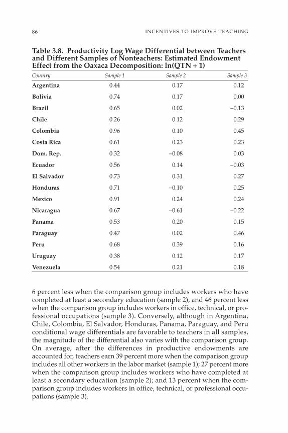
6 percent less when the comparison group includes workers who havecompleted at least a secondary education (sample 2), and 46 percent lesswhen the comparison group includes workers in office, technical, or pro-fessional occupations (sample 3). Conversely, although in Argentina,Chile, Colombia, El Salvador, Honduras, Panama, Paraguay, and Peruconditional wage differentials are favorable to teachers in all samples,the magnitude of the differential also varies with the comparison group.On average, after the differences in productive endowments areaccounted for, teachers earn 39 percent more when the comparison groupincludes all other workers in the labor market (sample 1); 27 percent morewhen the comparison group includes workers who have completed atleast a secondary education (sample 2); and 13 percent when the com-parison group includes workers in office, technical, or professional occu-pations (sample 3).
86 INCENTIVES TO IMPROVE TEACHING
Table 3.8. Productivity Log Wage Differential between Teachersand Different Samples of Nonteachers: Estimated EndowmentEffect from the Oaxaca Decomposition: ln(QTN + 1)Country Sample 1 Sample 2 Sample 3
Argentina 0.44 0.17 0.12
Bolivia 0.74 0.17 0.00
Brazil 0.65 0.02 −0.13
Chile 0.26 0.12 0.29
Colombia 0.96 0.10 0.45
Costa Rica 0.61 0.23 0.23
Dom. Rep. 0.32 −0.08 0.03
Ecuador 0.56 0.14 −0.03
El Salvador 0.73 0.31 0.27
Honduras 0.71 −0.10 0.25
Mexico 0.91 0.24 0.24
Nicaragua 0.67 −0.61 −0.22
Panama 0.53 0.20 0.15
Paraguay 0.47 0.02 0.46
Peru 0.68 0.39 0.16
Uruguay 0.38 0.12 0.17
Venezuela 0.54 0.21 0.18
87ARE TEACHERS WELL PAID?
Again, the fact that conditional wage differentials vary with the defini-tion of the comparison group suggests that—even though one controlsfor differences in observable productive endowments and socioeconomiccharacteristics—there are differences in unobserved heterogeneitybetween teachers and nonteachers that are related to both the wages andthe decision to work as a teacher.
In summary, when I combine my two estimates of the conditional wagedifferential, the results suggest that—after the differences in observed pro-ductive endowments are accounted for—teachers receive higher wagesthan nonteachers in Argentina, Chile, Colombia, El Salvador, Honduras,Panama, Paraguay, and Peru. They receive lower wages in Nicaragua.However, the sensitivity of the magnitudes of the conditional wage differ-entials to the alternative definitions of the comparison group also suggeststhat teachers are not a random sample of the population. Thus the esti-mates may be biased because of the presence of unobserved heterogeneity.In the cases of Bolivia, Brazil, Costa Rica, the Dominican Republic,Ecuador, Mexico, Uruguay, and Venezuela, it is not possible to determinewhether teachers receive higher or lower wages without choosing a par-ticular comparison group and method.
Differences in the Structure of Returns
The Oaxaca decomposition allows one not only to decompose the grosswage differential into an endowment and a price effect, but also to identifywhich returns explain most of the conditional wage differential: schooling,potential experience, women’s wage premium, rural residence wage pre-mium, or initial wage.
Returns to SchoolingFigure 3.7 shows how much the difference in the returns to schooling con-tributes to the conditional wage differential between teachers and differentsamples of nonteachers. In almost all countries, teachers’ returns for anadditional year of schooling are lower. When teachers are compared withall other workers in the labor market (sample 1), only Venezuela is anexception. When they are compared with workers who have completedat least a secondary education (sample 2), only Chile is an exception. Whenthey are compared with workers in office, technical, or professional occu-pations (sample 3), only Venezuela is an exception. An additional year ofschooling increases the wages of teachers by 5 percent on average, whereasit increases the wages of nonteachers by 8 percent to 14 percent, depend-ing on the sample used.
It is important to note that, in most Latin American countries, significantdifferences exist in the character and quality of teachers’ education comparedwith other types of higher education. Therefore, it may be inappropriate to

conclude that teachers would receive better returns for their education inother sectors of the labor market.
Potential ExperienceFigure 3.8 shows how much the difference in returns to 5 years of potentialexperience contributes to the conditional wage differential between teach-ers and different samples of nonteachers. The results reveal that, in thecases of El Salvador, Honduras, Nicaragua, Paraguay, and Peru, teachers’expected wage growth after 5 years is higher compared with that of allother workers in the labor market (sample 1); with that of workers who
88 INCENTIVES TO IMPROVE TEACHING
El Salvador
Bolivia
Brazil
Paraguay
Dom. Rep.
Peru
Panama
Honduras
Costa Rica
Ecuador
Colombia
Uruguay
Argentina
Mexico
Venezuela
Nicaragua
Chile
Sample 1 Sample 2 Sample 3
–3 –2 –1 0 1–3 –2 –1 0 1–2 –1 0 1
Note: Sample 1 includes all workers other than teachers who declared their labor earnings and hours worked. Sample 2 restricts sample 1 to those who have completed at least a secondary education. Sample 3 includes all workers other than teachers who are in office, technical, or professional occupations.
Figure 3.7. Contribution of the Difference in the Return to Schooling to the Conditional Log Wage Differential

89ARE TEACHERS WELL PAID?
Uruguay
Costa Rica
Chile
Panama
Bolivia
Argentina
Mexico
Brazil
Ecuador
Colombia
Dom. Rep.
Venezuela
Paraguay
Nicaragua
Honduras
Peru
El Salvador
Sample 1 Sample 2 Sample 3
–2 –1 0 1 2–2 –1 0 1 2–2 –1 0 21
Note: Sample 1 includes all workers other than teachers who declared their labor earnings and hours worked. Sample 2 restricts sample 1 to those who have completed at least a secondary education. Sample 3 includes all workers other than teachers who are in office, technical, or professional occupations.
Figure 3.8. Contribution of the Difference in the Returns toPotential Experience to the Conditional Log Wage Differential
have completed at least a secondary education (sample 2); and with that ofworkers in office, technical, and professional occupations (sample 3). In thecase of the Dominican Republic, Mexico, and Venezuela, the contribution ofthe difference in returns to potential experience depends on the definitionof the comparison group.
Conversely, in the cases of Argentina, Bolivia, Brazil, Chile, Colombia,Costa Rica, Ecuador, Panama, and Uruguay, teachers’ expected wagegrowth after 5 years is lower compared with that of all other workers inthe labor market (sample 1); with that of workers who have completed atleast a secondary education (sample 2); and with that of workers in office,technical, and professional occupations (sample 3).

90 INCENTIVES TO IMPROVE TEACHING
One would expect a steeper wage–age profile for teachers given that,in most Latin American countries, job experience is the most important deter-minant for promotions. However, note that, although age may be a goodproxy of the years of job experience, the correlation between age and jobexperience may differ between teachers and nonteachers. For example,because teachers include a greater percentage of women, and becausewomen tend to spend longer periods out of the labor force, potential experi-ence may be a better proxy of job experience in the comparison groups.
Sex DiscriminationFigure 3.9 shows how much the difference in women’s wage premiumscontributes to the conditional wage differential between teachers and dif-ferent samples of nonteachers. For most countries (excluding Hondurasand Nicaragua), the difference in women’s wage premiums contributespositively to the conditional wage differential. This fact suggests that theeducation sector does not discriminate against women, or at least that,if it does, the discrimination is lower compared with that in other sectorsof the labor market. However, we must note that the contribution ofwomen’s wage premiums to the conditional wage differential is secondorder compared with the contribution of the returns to education orpotential experience.
In the teacher sample, the estimated women’s wage premiums are neg-ative and significant in Argentina, Brazil, Chile, Colombia, Ecuador, Hon-duras, Mexico, and Nicaragua (from −0.07 to −0.31). The DominicanRepublic, Paraguay, Peru, and Uruguay exhibit estimates that are also neg-ative but not statistically significant (from −0.07 to −0.16). Costa Rica, ElSalvador, Panama, and Venezuela exhibit positive but not statistically sig-nificant estimates (from 0 to 0.04). Bolivia is the only country where theestimates were positive and statistically significant (0.13). Conversely, con-sistent with the presence of discrimination against women in the labormarket, the estimated women’s wage premiums are negative and statisti-cally significant in all nonteacher samples and countries.
Although it is possible that there is discrimination against women in theeducation labor market, it is also possible that the dummy for women iscorrelated with other unobservable characteristics, particularly in the caseof teachers. As noted earlier, because a greater percentage of women areteachers, and because women tend to spend longer periods out of the laborforce, it may be the case that the dummy for women is capturing differ-ences associated with the levels of job experience (and not captured bythe age) instead of discrimination.
Rural ResidenceFigure 3.10 shows how much the difference in rural residence wage pre-miums contributes to the conditional wage differential between teachers
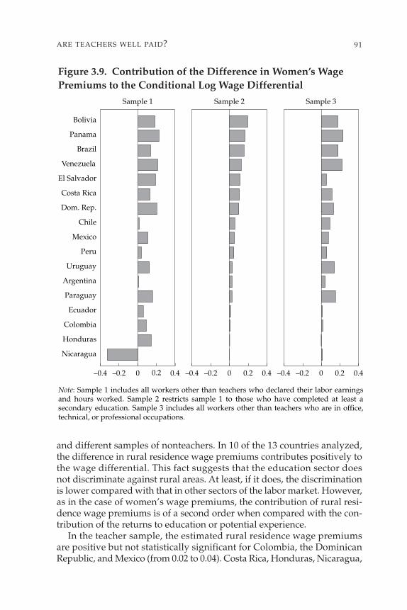
and different samples of nonteachers. In 10 of the 13 countries analyzed,the difference in rural residence wage premiums contributes positively tothe wage differential. This fact suggests that the education sector doesnot discriminate against rural areas. At least, if it does, the discriminationis lower compared with that in other sectors of the labor market. However,as in the case of women’s wage premiums, the contribution of rural resi-dence wage premiums is of a second order when compared with the con-tribution of the returns to education or potential experience.
In the teacher sample, the estimated rural residence wage premiumsare positive but not statistically significant for Colombia, the DominicanRepublic, and Mexico (from 0.02 to 0.04). Costa Rica, Honduras, Nicaragua,
91ARE TEACHERS WELL PAID?
Nicaragua
Honduras
Colombia
Ecuador
Paraguay
Argentina
Uruguay
Peru
Mexico
Chile
Dom. Rep.
Costa Rica
El Salvador
Venezuela
Brazil
Panama
Bolivia
Sample 1 Sample 2 Sample 3
–0.4 –0.2 0 0.2 0.4–0.4 –0.2 0 0.2 0.4–0.4 –0.2 0 0.40.2
Note: Sample 1 includes all workers other than teachers who declared their labor earnings and hours worked. Sample 2 restricts sample 1 to those who have completed at least a secondary education. Sample 3 includes all workers other than teachers who are in office, technical, or professional occupations.
Figure 3.9. Contribution of the Difference in Women’s WagePremiums to the Conditional Log Wage Differential

92 INCENTIVES TO IMPROVE TEACHING
Honduras
El Salvador
Ecuador
Brazil
Colombia
Bolivia
Costa Rica
Mexico
Nicaragua
Panama
Dom. Rep.
Peru
Paraguay
Sample 1 Sample 2 Sample 3
–0.4 –0.2 0.0 0.2 0.4–0.4 –0.2 0.0 0.2 0.4–0.2 0.0 0.2 0.4
Note: Sample 1 includes all workers other than teachers who declared their labor earnings and hours worked. Sample 2 restricts sample 1 to those who have completed at least a secondary education. Sample 3 includes all workers other than teachers who are in office, technical, or professional occupations.
Figure 3.10. Contribution of the Difference in Rural ResidenceWage Premium to the Conditional Log Wage Differential
Panama, Paraguay, and Peru exhibit negative but not statistically signifi-cant estimates, whereas Bolivia, Brazil, Ecuador, and El Salvador exhibitnegative and statistically significant estimates (from −0.08 to −0.25). How-ever, all countries exhibit negative rural residence wage premiums in thenonteacher samples, which are statistically significant in almost all cases.
Note that the negative estimates for rural wage premiums in the teachersample cannot be related to the presence of wage discrimination againstteachers who work in rural areas. Most schools in rural areas in LatinAmerica and the Caribbean are public, and in the public sector, there isgenerally no differentiation between urban and rural areas with respectto wages. If such differentiation does exist, wages are higher in rural areas.Therefore, it is possible that the rural dummy is also correlated with otherunobservable characteristics. For example, the negative estimates of ruralwage premiums may be related to the lower levels of qualification ofteachers in rural areas that are not captured by the years of schooling orpotential experience.
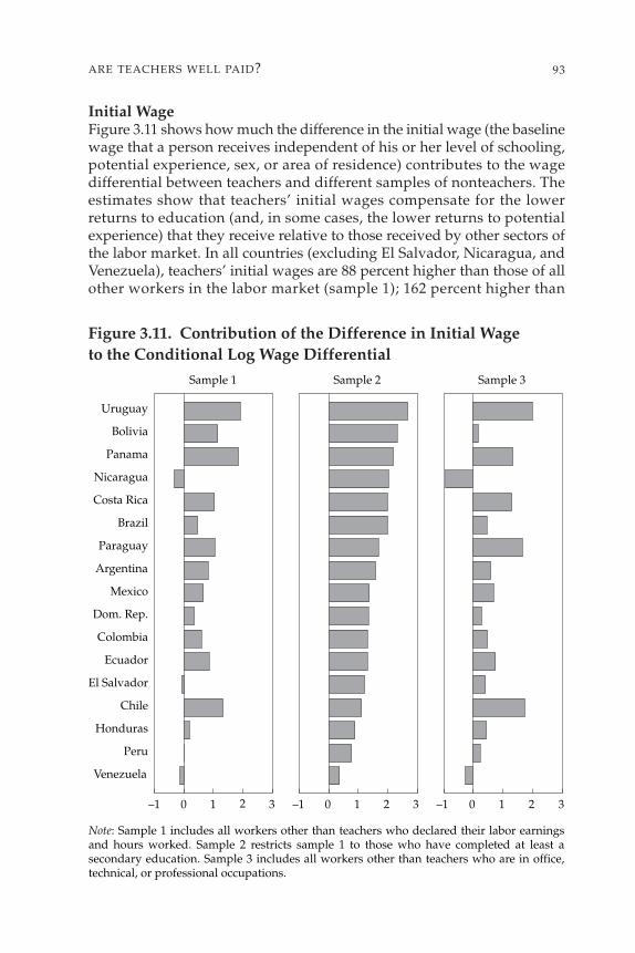
Initial WageFigure 3.11 shows how much the difference in the initial wage (the baselinewage that a person receives independent of his or her level of schooling,potential experience, sex, or area of residence) contributes to the wagedifferential between teachers and different samples of nonteachers. Theestimates show that teachers’ initial wages compensate for the lowerreturns to education (and, in some cases, the lower returns to potentialexperience) that they receive relative to those received by other sectors ofthe labor market. In all countries (excluding El Salvador, Nicaragua, andVenezuela), teachers’ initial wages are 88 percent higher than those of allother workers in the labor market (sample 1); 162 percent higher than
93ARE TEACHERS WELL PAID?
Venezuela
Peru
Honduras
Chile
El Salvador
Ecuador
Colombia
Dom. Rep.
Mexico
Argentina
Paraguay
Brazil
Costa Rica
Nicaragua
Panama
Bolivia
Uruguay
Sample 1 Sample 2 Sample 3
–1 0 1 2 3–1 0 1 2 3–1 0 1 32
Note: Sample 1 includes all workers other than teachers who declared their labor earnings and hours worked. Sample 2 restricts sample 1 to those who have completed at least a secondary education. Sample 3 includes all workers other than teachers who are in office, technical, or professional occupations.
Figure 3.11. Contribution of the Difference in Initial Wage to the Conditional Log Wage Differential

those of workers who have completed at least a secondary education(sample 2); and 86 percent higher than workers in office, technical, or pro-fessional occupations (sample 3).
The fact that teachers’ hourly wages are independent of their levels ofschooling, years of potential experience, sex, area of residence, and distrib-ution of observed productive endowments explains why teachers’ wagedistributions are much more compressed. The coefficient of variation forthe wage distribution is 58 percent for the teacher sample; 99 percent forall other workers of the labor market (sample 1); 91 percent for those work-ers who have completed at least a secondary education (sample 2); and 85percent for those workers in office, technical, and professional occupations(sample 3).
Although higher initial wages and lower returns are important inexplaining why we observe less inequality in teachers’ wage distribution,the distribution of productive endowments is also more homogenous forthe teacher sample. For example, the standard deviation of years ofschooling levels is around 2.3 years for the teacher sample; 4.5 yearsfor all other workers in the labor market (sample 1); 2.1 for all other work-ers who have completed at least a secondary education (sample 2); and3.5 years for workers in office, technical, and professional occupations(sample 3).
Note that the variation in observed productive endowments accountsfor only a small proportion of the total variation in teachers’ wages. The R2
coefficients of the estimated wage regressions for teachers are between 5 percent and 37 percent, and they are around 18 percent on average. Thisresult suggests that unobserved heterogeneity plays an important role inthe analysis of the teachers’ relative wages.
Unobserved Heterogeneity and Wage Differentials
To compare people with similar levels of unobserved heterogeneity, I usedLeast Absolute Deviation (LAD) estimates to calculate conditional wagedifferentials for different quantiles of the conditional wage distribution.Figure 3.12 and table 3.9 present the estimates. Following Juhn, Murphy,and Pierce (1993), I interpreted the position in the conditional distribu-tion of the logarithm of the wage as a measure of unobserved ability.
The estimates suggest that the answer to the question of whetherteachers are well paid or not depends on the teachers’ positions in theconditional wage distribution. After differences in productive endow-ments are accounted for, wage differentials tend to be positive and higherfor low-ability teachers (teachers in the lower parts of the conditionalwage distribution), whereas wage differentials tend to be zero or negativefor high-ability teachers (teachers in the upper part of the conditionalwage distribution).
94 INCENTIVES TO IMPROVE TEACHING

95ARE TEACHERS WELL PAID?
Bolivia
Venezuela
Argentina
Uruguay
Panama
Brazil
Paraguay
Mexico
Peru
Colombia
Ecuador
Nicaragua
Dom. Rep.
Costa Rica
1.0 0.5 0.0 –0.5 –1.0
10th 25th 50th 75th 90th
TeachersNonteachers
Figure 3.12. Conditional Log Wage Differential between Teachersand Nonteachers by Quantile of the Conditional Wage Distribution
On average, after differences in productive endowments are accountedfor, teachers in the 10th percentile of the conditional wage distributionreceive wages 60 percent higher than their counterparts in the same per-centile, teachers in the 25th percentile receive wages 43 percent higher, andteachers in the 50th percentile receive wages 24 percent higher (except inNicaragua, where teachers’ wages are 20 percent lower). At the other sideof the conditional wage distribution, teachers in the 75th percentile receivewages at least as high as nonteachers (slightly higher in Argentina, Chile,Colombia, Costa Rica, El Salvador, Honduras, Mexico, Panama, Paraguay,and Peru and lower in Bolivia, Brazil, the Dominican Republic, Ecuador,Uruguay, and Venezuela). Teachers in the 90th percentile receive wages14 percent lower (except in Argentina, Colombia, El Salvador, Honduras,Mexico, and Paraguay).

Conclusions
Teachers’ value added to the education production process is directlyrelated to their overall quality. Teachers’ quality is, in turn, determinedby what type of people are attracted to the profession, what incentivesthey have to perform on the job, and whether highly productive teacherswill stay. Recruitment, performance, and retention are directly related toteachers’ opportunity cost (that is, the wage teachers would receive in analternative occupation).
It is important to note that although age is (arguably) the most importantfactor that affects recruitment, performance, and retention, it is not the onlyone. The stability of the job, the number of hours required at work, theflexibility of the schedule, and all kinds of nonmonetary benefits (vacations,
96 INCENTIVES TO IMPROVE TEACHING
Table 3.9. Conditional Log Wage Differential between Teachersand Sample 1 of Nonteachers by QuantileCountry 10th 25th 50th 75th 90th Mean
Argentina 0.40 0.30 0.19 0.10 0.06 0.21
Bolivia 0.84 0.48 0.18 −0.14 −0.50 0.14
Brazil 0.33 0.25 0.07 −0.11 −0.31 0.04
Chile 1.19 0.82 0.43 0.14 −0.12 0.69
Colombia 0.47 0.35 0.29 0.24 0.13 0.29
Costa Rica 0.35 0.24 0.25 0.10 −0.02 0.17
Dom. Rep. 0.27 0.23 0.13 −0.05 −0.18 0.05
Ecuador 0.42 0.31 0.14 −0.03 −0.23 0.10
El Salvador 0.92 0.68 0.51 0.31 0.08 0.47
Honduras 0.86 0.67 0.43 0.25 0.03 0.44
Mexico 0.61 0.52 0.41 0.26 0.06 0.35
Nicaragua 0.36 0.09 −0.20 −0.59 −0.86 −0.23
Panama 0.69 0.56 0.33 0.10 −0.09 0.32
Paraguay 0.58 0.47 0.21 0.02 0.37 0.32
Peru 0.84 0.63 0.42 0.16 −0.18 0.40
Uruguay 0.58 0.38 0.11 −0.15 −0.33 0.13
Venezuela 0.55 0.32 0.17 −0.02 −0.30 0.16

in-kind payments, and so forth) are also important dimensions of the laborcontract. Therefore, the positive or negative sign and the magnitude of theteachers’ relative wage may be affected by the inclusion or exclusion ofthose factors. For example, because teachers tend to work fewer hours andhave longer periods of vacation, earnings differentials that account forthose factors will be higher than hourly wage differentials. This chapteranalyzes wage differentials by taking labor supply as given and excludingall kinds of nonmonetary benefits.
The estimates of teachers’ relative wages rely on data from recenthousehold surveys. When using household surveys, one should bear inmind that teachers’ relative wages and the structure of returns obtainedfrom alternative sources of information may be different from thosedescribed in this chapter. One should also be cautious when making inter-national comparisons, because household surveys usually have importantdifferences in the sample design, the definition of some variables (partic-ularly income), and the quality.
The data reveal that not only the direction, but also the magnitude ofthe unconditional and conditional wage differential depends on the defi-nition of the comparison group. The fact that unconditional wage differ-entials vary with the definition of the comparison group is obvious,because significant differences exist in productive endowments betweenteachers and alternative definitions of nonteachers. Therefore, uncondi-tional wage differentials tend to be higher when teachers are comparedwith workers who have lower productive endowments. Differences inobserved productive endowments account for 75 percent of the grosswage differential when teachers are compared to all other workers in thelabor market (sample 1); for 50 percent when they are compared withworkers with at least a secondary education (sample 2); and for 64 per-cent when they are compared to workers in office, technical, and profes-sional occupations (sample 3).
However, the fact that conditional wage differentials are also sensitiveto the definition of the comparison group suggests that—even thoughone controls for differences in observable productive endowments andsocioeconomic characteristics—differences in unobserved characteristicsare related to wages and the decision to work as a teacher. The sign andmagnitude of the adjusted or conditional wage differential also depend onthe definition of the comparison group. This result suggests that eventhough differences in observable productive endowments and socioeco-nomic characteristics are accounted for, differences in unobserved hetero-geneity exists between teachers and nonteachers and are related to bothwages and the decision to work as a teacher. When one combines the twoalternative estimates of the conditional wage differential, the results suggestthat teachers receive higher wages than nonteachers in Argentina, Chile,
97ARE TEACHERS WELL PAID?

Colombia, El Salvador, Honduras, Panama, Paraguay, and Peru; theyreceive lower wages in Nicaragua. In the cases of Bolivia, Brazil, CostaRica, the Dominican Republic, Ecuador, Mexico, Uruguay, and Venezuela,it is not possible to determine whether teachers receive higher or lowerwages without choosing a particular comparison group and method.
About the structure of returns, the data reveal that, in most Latin Ameri-can countries, the difference in initial wages compensates for the lower returnto education (and, in some cases, the lower return to potential experience)that teachers receive. Being a woman and living in a rural area also con-tribute positively to the conditional wage differential. This result suggeststhat the education sector does not discriminate against women or thosein rural areas. If it does, the discrimination is lower compared with thatfound in other sectors of the labor market. However, one must note thatthe contribution of these factors to the conditional wage differential is ofa second order when compared with the contribution of the returns toeducation or potential experience.
Note that, when analyzing teachers’ relative structure of returns, oneshould be cautious about the presence of unobserved heterogeneity. It maybe the case that the estimated coefficients are biased because of correla-tion between productive endowments and unobserved characteristics,particularly in the case of teachers. For example, because a higher per-centage of women work as teachers and because women tend to spendlonger periods out of the labor force, the lower returns to potential expe-rience and the negative wage premiums estimated for female teachers maybe capturing differences in the levels of job experience and not necessar-ily the flatter wage–age profiles or sex discrimination in the educationsector. It may also be the case that the negative estimates for rural wagepremiums for teachers are capturing the lower levels of qualification ofteachers in the rural area and not necessarily the wage discriminationagainst teachers in those areas.
To compare people with similar levels of unobserved heterogeneity, I usedLeast Absolute Deviation (LAD) estimates to calculate conditional wage dif-ferentials for different quantiles of the conditional wage distribution, and Iinterpreted the position in the conditional distribution of the logarithm of thewage as a measure of unobserved ability. The estimates suggest that theanswer to the question of whether teachers are well paid depends on theteachers’ position in the conditional wage distribution. After differences inproductive endowments are accounted for, wage differentials tend to bepositive and higher for low-ability teachers, and they are zero or negative forhigh-ability teachers. On average, after differences in productive endow-ments are accounted for, teachers in the 10th percentile of the conditionalwage distribution receive wages 60 percent higher than their counter-parts in the same percentile, teachers in the 25th percentile receivewages 43 percent higher, and teachers in the 50th percentile receive
98 INCENTIVES TO IMPROVE TEACHING

wages 24 percent higher (except in Nicaragua, where teachers’ wagesare 20 percent lower). At the other side of the conditional wage distrib-ution, teachers in the 75th percentile receive wages at least as high asnonteachers (slightly higher in Argentina, Chile, Colombia, Costa Rica,El Salvador, Honduras, Mexico, Panama, Paraguay, and Peru and lowerin Bolivia, Brazil, the Dominican Republic, Ecuador, Uruguay, andVenezuela). Finally, teachers in the 90th percentile receive wages 14 percentlower (except in Argentina, Colombia, El Salvador, Honduras, Mexico,and Paraguay).
99ARE TEACHERS WELL PAID?


References
Carnoy, M., and P. McEwan. 1997. “La educación y el mercado laboral enHonduras.” Report for the Secretaría de Educación–ASED Project.Stanford University, Stanford, Calif. Processed.
ECLAC (Economic Commission for Latin America and the Caribbean).1999. Panorama social de América Latina 1998. Santiago.
Grupo de Economistas y Asociados. 1998. “Análisis de las percepcionesmonetarias de los maestros de educación primaria.” Mexico City.Processed.
Juhn, C., Murphy, K. M., and Pierce, B. 1993. “Wage Inequality and theRise in Returns to Skill.” Journal of Political Economy 101: 410–42.
Koenker, R., and G. Bassett. 1978. “Regression Quantiles.” Econometrica46: 33–50.
Liang, X. 1999. “Teacher Pay in 12 Latin American Countries: How DoesTeacher Pay Compare to Other Professions, What Determines TeacherPay, and Who Are the Teachers?” Latin America and the CaribbeanRegion Human Development Department Paper 49. World Bank,Washington, D.C.
López-Acevedo, G., and A. Salinas. 2000. “Teachers’ Salaries and Profes-sional Profile in Mexico.” Latin America and the Caribbean Region,World Bank, Washington, D.C. Processed.
Mizala, A., and P. Romaguera. 2004. “Teachers’ Salary Structure andIncentives in Chile.” World Bank, Washington D.C. Processed.
Mulcahy-Dunn, A., and G. Arcia. 1996. “Teachers’ Salaries and LivingStandards in Ecuador.” Center for International Development,Research Triangle Institute, Research Triangle Park, N.C.
Oaxaca, R., and M. Ransom. 1994. “On Wage Discrimination and the Decomposition of Wage Differentials.” Journal of Econometrics16(1): 5–21.
101
Piras, C., and W. Savedoff. 1998. “How Much Do Teachers Earn?” IDB Work-ing Paper 375. Inter-American Development Bank, Washington, D.C.
Psacharopoulos, G., J. Valenzuela, and M. Arends. 1996. “Teacher Salariesin Latin America: A Review.” Economics of Education Review 15(4): 401–6.
Santibáñez, L. 2002. “¿Están los maestros en México mal pagados? Esti-mado de los salarios relativos del magisterio.” Revista Latinoamericana deEstudios Educativos 32(2): 9–41.
Urquiola, M., W. Jiménez, W. Hernani, and M. L. Talavera. 2000. “Losmaestros en Bolivia: Impacto, incentivos y desempeño.” Maestrías parael Desarrollo Universidad Católica Boliviana, La Paz.
Vegas, E., W. Experton, and L. Pritchett. 1998. “Teachers in Argentina: Under-(Over) Worked? Under- (Over) Paid?” World Bank, Washington, D.C.Processed.
102 INCENTIVES TO IMPROVE TEACHING

4Teachers’ Salary Structure
and Incentives in Chile
Alejandra Mizala and Pilar RomagueraCenter for Applied Economics, Department of Industrial Engineering,
University of Chile
The purpose of this chapter is to analyze the level, trends, and structure ofteachers’ salaries in Chile and to compare the salaries with those of otherworkers who have similar characteristics. Analyzing what is going on withteachers’ salaries is interesting because, in many countries—and Chile is noexception—teachers’ salaries are often perceived to be low and less thanthose of other professionals. If this perception were the case, it would havethree possible effects on the efficiency of the educational process.
First, lower salaries would affect the effort and the quality of teachers’work. Second, low salaries would negatively affect the quality of educationstudents and, therefore, the pool of future teachers. Third, it would be hardto keep good teachers in the profession, because they would seek betterincome elsewhere. Those effects would produce significant inefficiencies inthe educational process and negative effects in students’ learning.
A question that arises is why debate occurs more about teachers’ salariesthan about salaries of other kinds of workers. In particular, many studiesask whether teachers are underpaid. We think the explanation lies in thefact that, in education, the quality of teaching cannot be observed directlyand, therefore, teachers’ productivity cannot be directly measured either.This fact affects how teachers’ salaries are determined and structured.
One way of dealing with this issue is to introduce incentive systems thatmotivate teachers to give the best quality service they can. This approachrequires study not only of the level and structure of teachers’ salaries butalso of the incentives embedded within teachers’ salary structure.
This chapter is organized in the following manner. The first sectionbriefly summarizes the main characteristics of Chilean teachers. The second
103
We acknowledge the support of the World Bank. We are grateful for valuable commentsfrom Emiliana Vegas and the participants at the World Bank workshop on Teacher Qualityand Incentives in Latin America. We also thank Marcelo Henríquez for collaborating with us.

analyzes the institutional context of the teachers’ labor market. The thirdanalyzes trends in salaries from 1990 on. In the fourth section, we analyzehow salaries affect the behavior of those applying to study teaching. Thefifth section provides an econometric analysis of teachers’ salaries, whichmakes it possible to compare them with those of other similar workers. Inthe sixth section, we study the incentives implicit in the current salarystructure for teachers. The seventh section describes the National System ofPerformance Assessment (Sistema Nacional de Evaluación de Desempeñode los Establecimientos Educacionales, SNED) and offers a preliminaryassessment of the effect of the SNED on student’s outcomes. We examinethe SNED for two reasons. Until recently, it was the sole monetary incentiveassociated with evaluating teachers’ performance. Similarly, it is the soleincentive that evaluates teachers’ performance according to students’results on standardized tests. The eighth section presents the opinions ofteachers and principals about performance evaluation and monetary incen-tive payments associated with such evaluations, and the ninth section sum-marizes the conclusions.
Who Are Chile’s Teachers?
Figures from the Ministry of Education (MINEDUC) for 2001 indicate atotal of 146,918 teachers were in the country. Of those, 55 percent work inmunicipal (public) schools, 31 percent work in subsidized private schools,and the rest work in fee-paying private schools. Within this total group,86 percent of teachers work in urban schools. In terms of educational lev-els, 59 percent work in primary education, 27 percent work in secondaryeducation, 8 percent work in preschool education, 4 percent work in spe-cial education, and 1.6 percent work in adult education. In terms ofresponsibilities, 85.5 percent are classroom teachers, 6.5 percent are prin-cipals, 2.9 percent are principals of rural schools with fewer than threeteachers, and 3.5 percent are technical–pedagogical personnel.12
Education is dominated by women, with 70 percent of teachers beingwomen. Most are concentrated in preschool and primary education. Insecondary education, the distribution of men and women is more even.Despite the high percentage of women teachers, 51 percent of principalsare men; figures are similar for the leadership of the national teachers’association (Colegio de Profesores).
With respect to education and experience, the vast majority of teachers(90 percent) have a university degree. One-third (33 percent) have fewerthan 10 years of experience, 25 percent have 10 to 19 years of experience,27 percent have from 20 to 29 years of experience, and 15 percent have30 years of experience or more.
104 INCENTIVES TO IMPROVE TEACHING
12. The rest consist of unclassified others.

As with most countries, teachers work fewer hours than the averageChilean worker. Just 22 percent of teachers work 44 hours a week (thisamount is the maximum number of hours of work allowed with the sameemployer in the subsidized system) whereas the work week defined by theChilean Labor Code currently amounts to 48 hours per week and willfall to 44 hours in 2005. Of the remaining teachers, 35 percent work from 31 to 43 hours, 29 percent work 30 hours, and 15 percent work fewer than30 hours. Just 10 percent work more than 44 hours a week, which is con-sistent with the fact that just 13 percent of teachers work in more than oneschool.
How Teachers’ Salaries Are Determined
Chile has three types of schools: municipal (public) schools, subsidizedprivate schools, and fee-paying private schools.13 Therefore, the Chileanschool system has three types of employment contracts. The first type con-sists of those corresponding to the municipal sector, governed by theTeachers’ Statute (Estatuto Docente) established in 1991.14 The second typeincludes those in the subsidized private sector, governed by the LaborCode, which covers all private sector workers, but for which certain rulesin the Teachers’ Statute are binding. Among the rules are minimumsalaries, length of the working day, legal holiday periods, and termination.Finally, the third type of contracts is those in the fee-paying private sec-tor, also governed by the Labor Code, but for which the rules in theTeacher Statute are not binding.15
In the case of municipal schools in Chile, the Teachers’ Statute estab-lishes a common salary structure that is based on the Basic National Wage(Remuneración Básica Mínima Nacional, or RBMN) per teaching hour.This basic wage is increased by a series of allowances, many of whichare linked to the RBMN. Those allowances reflect years of experience,responsibility, training, and work in difficult conditions, among otherthings.
105TEACHERS’ SALARY STRUCTURE AND INCENTIVES IN CHILE
13. Municipal schools are financed through a per student subsidy that is provided by thestate and run by municipalities (local governments); they serve some 56 percent of enroll-ment. Subsidized private schools are financed by the per student subsidy that is providedby the state but are owned and operated by the private sector; they account for 34 percent ofenrollment. Fee-paying private schools operate on the basis of fees paid by parents and rep-resent approximately 10 percent of enrollment. For more information about the Chileaneducation system, see Mizala and Romaguera (2000b).
14. In the early 1980s, the Chilean education system was decentralized, with publicschools becoming dependent on municipal governments. Teachers thus ceased to be publicemployees and came under the private Labor Code. With the return of democratic rule, a spe-cial statute was created that defined new labor conditions for teachers.
15. See Mizala and others (2002) for a detailed analysis of the different types of teachers’contracts in Chile.
In the municipal sector, control over contracts and salaries is, nonetheless,centralized in the Ministry of Education. Likewise, centralized collectivebargaining is not established by law but is a consequence of the creation ofa national scale that standardizes teachers’ pay. In practice, wage negotia-tions have the characteristics of a bilateral monopoly (González 1998).
In the private sector, teachers enjoy collective bargaining rights accord-ing to private sector regulations, although parties may agree to functionunder the rules governing the municipal sector.
As a result of the Teachers’ Statute of 1991, the number of studentswhom schools managed to retain in their classrooms ceased to affect teach-ers’ job security. For this reason, Law 19410 of 1995 attempted to restoresome flexibility to the system. This legislation abolished lifetime employ-ment, making it possible to adjust staffing, to transfer teachers betweenschools in the same municipality, to rationalize resources, and even tomerge schools. In addition, the law introduced periodic competitions formanagement posts in municipal schools, which is important becauseschool principals can exert leadership that has a significant effect on aschool’s results.
In addition, the wage agreement that ended the dispute between theteachers’ union and the Ministry of Education in 1994 established a bonuspayment that was unrelated to teachers’ years of service but was inverselyproportional to excess staffing levels in the school or municipality. Thislegislation also set up the SNED, which awards an excellence bonus tothe best schools in each region of the country.16 Also, in 2000, a parallelteaching excellence bonus (Asignación de Excelencia Pedagógica) was addedfor those teaching the first 4 years of primary education. This bonus con-sists of a voluntary, individual evaluation that is associated with a moneyaward. To receive this award, teachers must successfully pass knowledge-based examinations, present their curricula, and submit a sample record-ing of a class they have taught.
The shift toward more flexibility has been difficult because the teachers’association has embraced the Teachers’ Statute as an historic aspirationthat protects teachers from job insecurity and arbitrary actions by admin-istrators.17 However, in recent years and independent of the teachers’ asso-ciation stance, signs of a change have been evident in teachers’ attitudetoward greater acceptance of elements such as evaluation and payment forperformance (see last section of this chapter). This change is importantbecause, for good management of human and financial resources, it is nec-essary to design more flexible labor regulations that make managerialefficiency possible and that encourage the improvements required for edu-cational quality.
106 INCENTIVES TO IMPROVE TEACHING
16. See Mizala and Romaguera (2002) for further details on the SNED.17. For more details, see Belleï (2001).
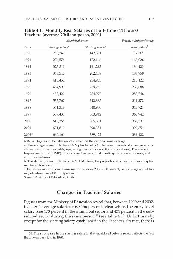
Table 4.1. Monthly Real Salaries of Full-Time (44 Hours) Teachers (average Chilean pesos, 2001)
Municipal sector Private subsidized sector
Years Average salarya Starting salaryb Starting salaryb
1990 258,242 142,591 73,337
1991 276,574 172,166 160,026
1992 323,311 191,293 184,123
1993 363,540 202,458 187,950
1994 413,452 234,933 210,122
1995 454,991 259,263 253,888
1996 488,420 284,977 283,746
1997 533,762 312,885 311,272
1998 561,318 340,970 340,721
1999 589,431 363,942 363,942
2000 615,368 385,331 385,331
2001 631,813 390,354 390,354
2002c 660,161 389,422 389,422
Note: All figures in the table are calculated on the national zone average.a. The average salary includes RBMN plus benefits (10 two-year periods of experience plusallowances for responsibility, upgrading, performance, difficult conditions), ProfessionalImprovement Unit (UMP), proportional bonuses, total handicap, excellence bonuses, andadditional salaries.b. The starting salary includes RBMN, UMP base; the proportional bonus includes comple-mentary allowances.c. Estimates, assumptions: Consumer price index 2002 = 3.0 percent; public wage cost of liv-ing adjustment in 2002 = 3.0 percent.Source: Ministry of Education, Chile.
Changes in Teachers’ Salaries
Figures from the Ministry of Education reveal that, between 1990 and 2002,teachers’ average salaries rose 156 percent. Meanwhile, the entry-levelsalary rose 173 percent in the municipal sector and 431 percent in the sub-sidized sector during the same period18 (see table 4.1). Unfortunately,except for the starting salary established in the Teachers’ Statute, there is
107TEACHERS’ SALARY STRUCTURE AND INCENTIVES IN CHILE
18. The strong rise in the starting salary in the subsidized private sector reflects the factthat it was very low in 1990.
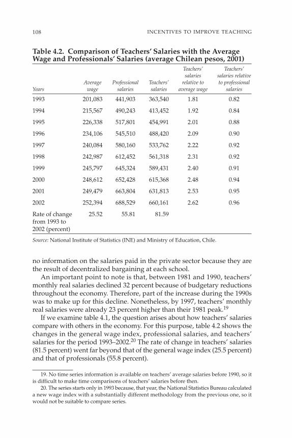
no information on the salaries paid in the private sector because they arethe result of decentralized bargaining at each school.
An important point to note is that, between 1981 and 1990, teachers’monthly real salaries declined 32 percent because of budgetary reductionsthroughout the economy. Therefore, part of the increase during the 1990swas to make up for this decline. Nonetheless, by 1997, teachers’ monthlyreal salaries were already 23 percent higher than their 1981 peak.19
If we examine table 4.1, the question arises about how teachers’ salariescompare with others in the economy. For this purpose, table 4.2 shows thechanges in the general wage index, professional salaries, and teachers’salaries for the period 1993–2002.20 The rate of change in teachers’ salaries(81.5 percent) went far beyond that of the general wage index (25.5 percent)and that of professionals (55.8 percent).
108 INCENTIVES TO IMPROVE TEACHING
19. No time series information is available on teachers’ average salaries before 1990, so itis difficult to make time comparisons of teachers’ salaries before then.
20. The series starts only in 1993 because, that year, the National Statistics Bureau calculateda new wage index with a substantially different methodology from the previous one, so itwould not be suitable to compare series.
Table 4.2. Comparison of Teachers’ Salaries with the AverageWage and Professionals’ Salaries (average Chilean pesos, 2001)
Teachers’ Teachers’salaries salaries relative
Average Professional Teachers’ relative to to professional Years wage salaries salaries average wage salaries
1993 201,083 441,903 363,540 1.81 0.82
1994 215,567 490,243 413,452 1.92 0.84
1995 226,338 517,801 454,991 2.01 0.88
1996 234,106 545,510 488,420 2.09 0.90
1997 240,084 580,160 533,762 2.22 0.92
1998 242,987 612,452 561,318 2.31 0.92
1999 245,797 645,324 589,431 2.40 0.91
2000 248,612 652,428 615,368 2.48 0.94
2001 249,479 663,804 631,813 2.53 0.95
2002 252,394 688,529 660,161 2.62 0.96
Rate of change 25.52 55.81 81.59from 1993 to 2002 (percent)
Source: National Institute of Statistics (INE) and Ministry of Education, Chile.

In 1993, teachers earned 1.8 times the income of an average worker withinthe economy whereas, by 2001, teachers were averaging 2.6 times thatincome. It is important to compare teachers’ earnings with those of otherworkers in the economy. If we compare teachers with professionals, whichis the occupational group whose salaries rose the most in this period (seeCowan and others 2002), we see that teachers’ salaries went from 82 per-cent of professionals’ salaries in 1993 to 96 percent in 2001. In other words, in2001, teachers on average earned practically the same as professionals.21
Table 4.3 compares the evolution of starting salaries for teachers in themunicipal sector22 with the minimum wage within the economy. Teachers’starting salary in 2002 was about 3.6 times the general minimum wage. Until1998, teachers’ starting salary grew more than the minimum wage everyyear. Only as the country’s growth slowed (in 1999) because of the effect of
109TEACHERS’ SALARY STRUCTURE AND INCENTIVES IN CHILE
21. At this point, we compared only the evolution of teachers’ salaries vis à vis other occu-pational groups. In a later section of the chapter, we analyzed teachers’ salaries comparedwith those of workers with similar characteristics.
22. From 1998 on, teachers’ minimum wage became the same for both the municipal andthe private subsidized sector.
Table 4.3. Comparison of Teachers’ Starting Salary with the National Minimum Wage (Chilean pesos of each year)
Municipal teachers’ Municipal
National Municipal starting salary National teachers’minimum teachers’ relative to minimum starting
Year wage starting salary minimum wage wage salary
1993 42,917 126,039 2.94
1994 49,588 163,024 3.29 15.54 29.34
1995 56,088 194,703 3.47 13.11 19.43
1996 62,750 229,793 3.66 11.88 18.02
1997 68,942 267,825 3.88 9.87 16.55
1998 76,708 306,794 4.00 11.26 14.55
1999 86,333 338,409 3.92 12.55 10.30
2000 96,042 372,057 3.87 11.25 9.94
2001 103,208 390,344 3.78 7.46 4.92
2002 111,420 401,087 3.60 7.96 2.75
Source: National Institute of Statistics (INE) and Ministry of Education, Chile.
Rate of annual change(percent)

the Asian crisis did teachers’ starting salary decrease to less than the gen-eral minimum wage.
Comparing teachers’ salaries in Chile with those of Organisation for Eco-nomic Co-operation and Development (OECD) and developing countriessuch as Chile provides a helpful context. Table 4.4 provides information for2001 on starting salaries and for teachers with 15 years’ experience in pri-mary and secondary education in U.S. dollars comparable for purchasingpower parity (PPP). The ratio between salaries and per capita gross domes-tic product (GDP) in each country is provided for the purpose of compari-son. When compared with the OECD mean, a selection of OECD countries,and some developing countries, Chile pays relatively similar salaries in rela-tion to its per capita GDP.
The rise in teachers’ salaries documented in table 4.1 explains a signifi-cant part of the increase in the Ministry of Education’s expenditures duringthe period 1990–2001 (see table 4.5). This increase is confirmed by notingthat total MINEDUC spending tripled between 1990 and 2001 and that thecorresponding expenditure on the per student voucher that the ministrypays to schools also tripled, maintaining a share of about 64 percent oftotal expenditure of the ministry during the decade.
The information available indicates that a significant part of theresources transferred by means of vouchers goes to pay teachers’ wages inthe municipal system.23 A study by González, Mizala, and Romaguera(2001) estimates that, on average at the municipal level, spending on remu-neration absorbs about 85 percent of voucher income, with a standard devi-ation of 14 percent.
Thus, one can conclude that the rise in teachers’ salaries does to a largedegree explain the significant rise in MINEDUC spending for the periodstudied.
Effect of Salary Trends on IndividualsApplying to Study Education
Despite a significant rise in teachers’ salaries in the past 13 years, teacherscontinue to say that their salaries are lower than those of other profes-sionals. This perception of low salaries is worrisome because it directlyaffects the quality of students entering education programs. All thingsbeing equal, the best students would prefer other fields.
In fact, from 1980 to 1994, the number of students training for the edu-cation field fell by about 43 percent (Ormeño 1996). Many reasons couldexplain this behavior, one being the plunge in teachers’ salaries, whichoccurred as monthly real salaries declined 32 percent in real terms during
110 INCENTIVES TO IMPROVE TEACHING
23. No information is available on what percentage of the subsidy received by privatesubsidized schools goes to salaries.
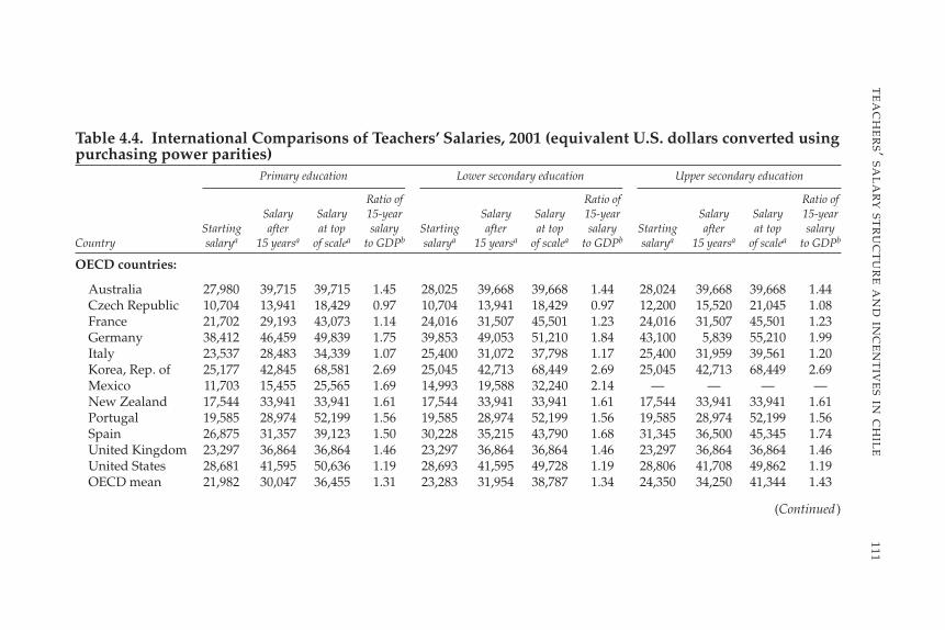
111T
EA
CH
ER
S’ SAL
AR
YST
RU
CT
UR
EA
ND
INC
EN
TIV
ES
INC
HIL
E
Table 4.4. International Comparisons of Teachers’ Salaries, 2001 (equivalent U.S. dollars converted usingpurchasing power parities)
Primary education Lower secondary education Upper secondary education
Ratio of Ratio of Ratio of Salary Salary 15-year Salary Salary 15-year Salary Salary 15-year
Starting after at top salary Starting after at top salary Starting after at top salary Country salarya 15 yearsa of scalea to GDPb salarya 15 yearsa of scalea to GDPb salarya 15 yearsa of scalea to GDPb
OECD countries:
Australia 27,980 39,715 39,715 1.45 28,025 39,668 39,668 1.44 28,024 39,668 39,668 1.44Czech Republic 10,704 13,941 18,429 0.97 10,704 13,941 18,429 0.97 12,200 15,520 21,045 1.08France 21,702 29,193 43,073 1.14 24,016 31,507 45,501 1.23 24,016 31,507 45,501 1.23Germany 38,412 46,459 49,839 1.75 39,853 49,053 51,210 1.84 43,100 5,839 55,210 1.99Italy 23,537 28,483 34,339 1.07 25,400 31,072 37,798 1.17 25,400 31,959 39,561 1.20Korea, Rep. of 25,177 42,845 68,581 2.69 25,045 42,713 68,449 2.69 25,045 42,713 68,449 2.69Mexico 11,703 15,455 25,565 1.69 14,993 19,588 32,240 2.14 — — — —New Zealand 17,544 33,941 33,941 1.61 17,544 33,941 33,941 1.61 17,544 33,941 33,941 1.61Portugal 19,585 28,974 52,199 1.56 19,585 28,974 52,199 1.56 19,585 28,974 52,199 1.56Spain 26,875 31,357 39,123 1.50 30,228 35,215 43,790 1.68 31,345 36,500 45,345 1.74United Kingdom 23,297 36,864 36,864 1.46 23,297 36,864 36,864 1.46 23,297 36,864 36,864 1.46United States 28,681 41,595 50,636 1.19 28,693 41,595 49,728 1.19 28,806 41,708 49,862 1.19OECD mean 21,982 30,047 36,455 1.31 23,283 31,954 38,787 1.34 24,350 34,250 41,344 1.43
(Continued)

112IN
CE
NT
IVE
ST
OIM
PR
OV
ET
EA
CH
ING
Table 4.4. International Comparisons of Teachers’ Salaries, 2001 (equivalent U.S. dollars converted usingpurchasing power parities) (Continued)
Primary education Lower secondary education Upper secondary education
Ratio of Ratio of Ratio of Salary Salary 15-year Salary Salary 15-year Salary Salary 15-year
Starting after at top salary Starting after at top salary Starting after at top salary Country salarya 15 yearsa of scalea to GDPb salarya 15 yearsa of scalea to GDPb salarya 15 yearsa of scalea to GDPb
Non-OECD countries:
Argentina 8,181 11,362 13,568 0.92 10,617 15,249 18,454 1.23 10,617 15,249 18,454 1.23Brazil 7,922 10,695 11,628 1.45 14,900 17,263 18,800 2.35 16,701 17,777 20,326 2.42Chile 11,631 12,902 17,310 1.37 11,631 12,902 17,310 1.37 11,631 13,487 18,107 1.43Peruc 5,597 5,597 5,597 1.22 5,536 5,536 5,536 1.20 5,536 5,536 5,536 1.20Philippines 10,777 11,896 12,811 3.06 10,777 11,896 12,811 3.06 10,777 11,896 12,811 3.06Uruguayd 5,734 6,872 8,295 0.76 5,734 6,872 8,295 0.76 6,240 7,378 8,801 0.82
Note: — = not available.a. With minimum training.b. Ratio of salary after 15 years of experience to GDP per capita.c. Year of reference 2000.d. Salaries for a position of 20 hours per week. Most teachers hold two positions.Source: OECD (2003).

113T
EA
CH
ER
S’ SAL
AR
YST
RU
CT
UR
EA
ND
INC
EN
TIV
ES
INC
HIL
E
Table 4.5. Total Expenditures of the Ministry of Education, 1990–2001, in Millions of 2001 Chilean pesos (and percentages)
Current transfers
Total Higher Scholarshipsc Researchd Total Total operational education Learning and and Other capital
Year expenditures expenditures Total Vouchers expenses resourcesa Programsb categorical aid development transfersexpenditurese
1990 556,474 53,349 502,783 355,070 88,645 589 1,448 45,531 9,465 2,035 341(%) (100) (9.6) (90.4) (63.8) (15.9) (0.1) (0.3) (8.2) (1.7) (0.4) (0.1)
1991 605,500 57,547 547,606 364,449 103,181 1,587 4,853 58,850 11,643 3,043 347(%) (100) (9.5) (90.4) (60.2) (17.0) (0.3) (0.8) (9.7) (1.9) (0.5) (0.1)
1992 685,751 66,194 612,973 403,986 109,519 2,406 2,056 74,217 10,931 9,859 6,584(%) (100) (9.7) (89.4) (58.9) (16.0) (0.4) (0.3) (10.8) (1.6) (1.4) (1.0)
1993 766,272 77,326 685,955 442,076 115,399 4,841 2,718 80,371 21,878 18,673 2,991(%) (100) (10.1) (89.5) (57.7) (15.1) (0.6) (0.4) (10.5) (2.9) (2.4) (0.4)
1994 831,749 76,310 755,405 501,751 120,108 2,747 4,328 82,935 25,416 18,121 33(%) (100) (9.2) (90.8) (60.3) (14.4) (0.3) (0.5) (10.0) (3.1) (2.2) (0.0)
1995 959,779 73,395 886,406 607,521 134,545 3,651 4,946 84,013 22,371 29,359 −22(%) (100) (7.6) (92.4) (63.3) (14.0) (0.4) (0.5) (8.8) (2.3) (3.1) (0.0)
1996 1,088,436 85,417 989,349 685,526 137,655 9,598 4,322 92,773 22,171 37,304 13,670(%) (100) (7.8) (90.9) (63.0) (12.6) (0.9) (0.4) (8.5) (2.0) (3.4) (1.3)
1997 1,221,888 91,870 1,100,674 777,612 142,758 8,882 6,580 90,635 23,265 50,942 19,343
(Continued)

114IN
CE
NT
IVE
ST
OIM
PR
OV
ET
EA
CH
ING
Table 4.5. Total Expenditures of the Ministry of Education, 1990–2001, in Millions of 2001 Chilean pesos (and percentages) (Continued)
Current transfers
Total Higher Scholarshipsc Researchd Total Total operational education Learning and and Other capital
Year expenditures expenditures Total Vouchers expenses resourcesa Programsb categorical aid development transfersexpenditurese(%) (100) (7.6) (90.8) (64.2) (11.8) (0.7) (0.5) (7.5) (1.9) (4.2) (1.6)
1998 1,335,315 106,363 1,206,914 836,220 157,648 11,793 9,832 97,002 24,662 69,757 22,038(%) (100) (8.0) (90.4) (62.6) (11.8) (0.9) (0.7) (7.3) (1.8) (5.2) (1.7)
1999 1,453,084 102,231 1,311,213 905,325 162,899 14,799 11,078 106,771 31,067 79,273 39,640(%) (100) (7.0) (90.2) (62.3) (11.2) (1.0) (0.8) (7.3) (2.1) (5.5) (2.7)
2000 1,570,038 97,614 1,386,094 988,769 164,912 20,377 9,295 112,945 26,173 63,623 86,330(%) (100) (6.2) (88.3) (63.0) (10.5) (1.3) (0.6) (7.2) (1.7) (4.1) (5.5)
2001 1,687,861 105,500 1,495,466 1,080,992 171,262 16,333 14,969 119,168 29,051 63,690 86,894(%) (100) (6.3) (88.6) (64.0) (10.1) (1.0) (0.9) (7.1) (1.7) (3.8) (5.1)
Note: MECE = Program for the Improvement of the Quality of Education; JUNAEB = National School Support and Scholarship Board; CONICYT =National Scientific and Technological Research Commission.a. The category includes textbooks, pedagogical resources, learning guides, classroom libraries, computers, and software. It does not include theexpenses of specific programs.b. Programs considered: Intercultural Bilingual Education; Drug Addiction and Alcoholism; Preschool Education; PEBM Workers, P900; Know YourChild; Elementary School MECE; Adult Education; Anticipation High School; Elementary Rural School.c. Scholarships considered: Indigenous Scholarships, Outstanding Students in Pedagogy, Secondary Education Scholarships and Categorical Aid,JUNAEB Scholarships, Higher Education Scholarships.d. Research here corresponds to research funds managed by CONICYTe. The category corresponds to capital contributions to the following: Full day school, High school for all, Higher Education infrastructure, andFinancial investment.
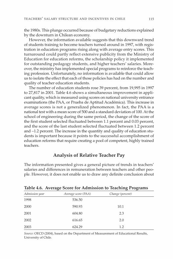
the 1980s. This plunge occurred because of budgetary reductions explainedby the downturn in Chilean economy.
However, the information available suggests that this downward trendof students training to become teachers turned around in 1997, with regis-tration in education programs rising along with average entry scores. Thisturnaround could partly reflect extensive publicity from the Ministry ofEducation for education reforms, the scholarship policy it implementedfor outstanding pedagogy students, and higher teachers’ salaries. More-over, the ministry has implemented special programs to reinforce the teach-ing profession. Unfortunately, no information is available that could allowus to isolate the effect that each of those policies has had on the number andquality of teacher education students.
The number of education students rose 39 percent, from 19,995 in 1997to 27,817 in 2001. Table 4.6 shows a simultaneous improvement in appli-cant quality, which is measured using scores on national university entranceexaminations (the PAA, or Prueba de Aptitud Académica). This increase inaverage scores is not a generalized phenomenon. In fact, the PAA is anational test with a mean score of 500 and a standard deviation of 100. At theschool of engineering during the same period, the change of the score ofthe first student selected fluctuated between 1.1 percent and 0.03 percent,and the score of the last student selected fluctuated between 1.2 percentand −1.2 percent. The increase in the quantity and quality of education stu-dents is important because it points to the successful accomplishment ofeducation reforms that require creating a pool of competent, highly trainedteachers.
Analysis of Relative Teacher Pay
The information presented gives a general picture of trends in teachers’salaries and differences in remuneration between teachers and other peo-ple. However, it does not enable us to draw any definite conclusion about
115TEACHERS’ SALARY STRUCTURE AND INCENTIVES IN CHILE
Table 4.6. Average Score for Admission to Teaching ProgramsAdmission year Average score (PAA) Change (percent)
1998 536.50
2000 590.93 10.1
2001 604.80 2.3
2002 616.65 2.0
2003 624.29 1.2
Source: OECD (2004), based on the Department of Measurement of Educational Results,University of Chile.

teachers’ pay compared to that of other workers. To be able to answer thequestion of whether teachers are overpaid or underpaid, we need to com-pare individuals with similar characteristics in terms of both human capitaland the jobs they perform.
It is, therefore, worthwhile to explore in more depth the differences be-tween teachers’ salaries and those of workers with similar characteristics.24
This analysis is based on data from the 1998 and 2000 Encuesta Nacionalde Caracterización Socioeconómica (National Socioeconomic Characteriza-tion Survey, or CASEN).25 The CASEN provides information on personalcharacteristics and individuals’ occupations. Table 4.7 gives information onthe income, human capital characteristics, and employment of teachers andnonteachers.26
One first important element to point out is that the hourly wageobtained from the 1998 CASEN is very similar to the one teachers declaredin a survey conducted by the authors of this study in Greater Santiagobetween November 1998 and January 1999.27 The hourly income from theirmain job was 1,849 pesos, according to the 1998 CASEN, and 1,805 pesos,according to the authors’ survey, both expressed in 1998 Chilean pesos(Ch pesos). The exchange rate stood at 460.3 pesos per U.S. dollar in 1998and 539.5 pesos per U.S. dollar in 2000.
The comparative analysis between teachers and other nonagriculturalworkers shows that hourly earnings from the main occupation are higherfor teachers than for other occupational groups. The same is true for totalearnings from the main job and earnings from all sources of labor income(see table 4.7).
116 INCENTIVES TO IMPROVE TEACHING
24. In recent years, several studies have examined the issue of teachers’ salaries in LatinAmerica; appendix 4.B summarizes the main findings. The results are mixed, indicatingthat no robust empirical evidence has proven that teachers receive lower salaries than acomparative group receives. Nonetheless, not all the studies control for workers’ character-istics. Many of the studies consist of a relatively aggregate comparison of salaries betweenteachers and other groups. Similarly, studies based on econometric analyses, except forthose of Piras and Savedoff (1998) and López-Acevedo and Salinas (2000), assume thatreturns are similar for teachers and other workers.
Other studies also address this issue for non–Latin American countries. For instance,Komenan and Grootaert (1990) study differences in pay for teachers and nonteachers in theCôte d’Ivoire, and Zymelman and DeStephano (1989) study teaching salaries in Sub-SaharanAfrican countries. In the case of the United States, this issue was analyzed by Ballou andPodgursky (1997), Flyer and Rosen (1996), and Lankford and Wyckoff (1997), among others.
25. The analysis using the 1998 CASEN survey was published in Mizala and Romaguera(2000a).
26. In 1998, 1,791 people employed as teachers in either elementary or secondary schoolswere identified according to their job and profession. The comparison group consists of58,006 people who were over the age of 15 years and who reported receiving income fromwork in either the public or private sector, excluding agricultural workers. In 2000, 2,394 peo-ple employed as teachers were identified; the comparison group comprised 51,917 people.
27. For more details about the survey, see Mizala and others (2002).
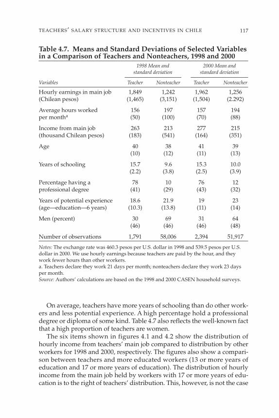
On average, teachers have more years of schooling than do other work-ers and less potential experience. A high percentage hold a professionaldegree or diploma of some kind. Table 4.7 also reflects the well-known factthat a high proportion of teachers are women.
The six items shown in figures 4.1 and 4.2 show the distribution ofhourly income from teachers’ main job compared to distribution by otherworkers for 1998 and 2000, respectively. The figures also show a compari-son between teachers and more educated workers (13 or more years ofeducation and 17 or more years of education). The distribution of hourlyincome from the main job held by workers with 17 or more years of edu-cation is to the right of teachers’ distribution. This, however, is not the case
117TEACHERS’ SALARY STRUCTURE AND INCENTIVES IN CHILE
Table 4.7. Means and Standard Deviations of Selected Variablesin a Comparison of Teachers and Nonteachers, 1998 and 2000
1998 Mean and 2000 Mean and standard deviation standard deviation
Variables Teacher Nonteacher Teacher Nonteacher
Hourly earnings in main job 1,849 1,242 1,962 1,256(Chilean pesos) (1,465) (3,151) (1,504) (2.292)
Average hours worked 156 197 157 194per montha (50) (100) (70) (88)
Income from main job 263 213 277 215(thousand Chilean pesos) (183) (541) (164) (351)
Age 40 38 41 39(10) (12) (11) (13)
Years of schooling 15.7 9.6 15.3 10.0(2.2) (3.8) (2.5) (3.9)
Percentage having a 78 10 76 12professional degree (41) (29) (43) (32)
Years of potential experience 18.6 21.9 19 23(age—education—6 years) (10.3) (13.8) (11) (14)
Men (percent) 30 69 31 64(46) (46) (46) (48)
Number of observations 1,791 58,006 2,394 51,917
Notes: The exchange rate was 460.3 pesos per U.S. dollar in 1998 and 539.5 pesos per U.S.dollar in 2000. We use hourly earnings because teachers are paid by the hour, and theywork fewer hours than other workers.a. Teachers declare they work 21 days per month; nonteachers declare they work 23 daysper month.Source: Authors’ calculations are based on the 1998 and 2000 CASEN household surveys.

118 INCENTIVES TO IMPROVE TEACHING
Log hourly income0 5 10 15
0
.2
.4
.6
.8
Source: CASEN 1998.
Perc
enta
ge o
f wor
kers
TeachersNonteachers (all)
Figure 4.1a. Hourly Income Distribution of Teachers and All Nonteachers, 1998
Log hourly income0 5 10 15
0
.2
.4
.6
.8
Source: CASEN 1998.
Perc
enta
ge o
f wor
kers
Teachers
Nonteachers (13)
Figure 4.1b. Hourly Income Distribution of Teachers and Nonteachers with 13 or More Years of Schooling, 1998

119TEACHERS’ SALARY STRUCTURE AND INCENTIVES IN CHILE
Log hourly income0 5 10 15
0
.2
.4
.6
.8
Source: CASEN 1998.
Perc
enta
ge o
f wor
kers
Teachers
Nonteachers (17)
Figure 4.1c. Hourly Income Distribution of Teachers and Nonteachers with 17 or More Years of Schooling, 1998
Log hourly income0 5 10 15
0
.2
.4
.6
.8
Source: CASEN 2000.
Perc
enta
ge o
f wor
kers
Teachers
Nonteachers (all)
Figure 4.2a. Hourly Income Distribution of Teachers and All Nonteachers, 2000

120 INCENTIVES TO IMPROVE TEACHING
Log hourly income0 5 10 15
0
.2
.4
.6
.8
Source: CASEN 2000.
Perc
enta
ge o
f wor
kers
Teachers
Nonteachers (13)
Figure 4.2b. Hourly Income Distribution of Teachers and Nonteachers with 13 or More Years of Schooling, 2000
Teachers
Nonteachers (17)
Log hourly income0 5 10 15
0
.2
.4
.6
.8
Source: CASEN 2000.
Perc
enta
ge o
f wor
kers
Figure 4.2c. Hourly Income Distribution of Teachers and Nonteachers with 17 or More Years of Schooling, 2000

when we compare teachers with workers with 13 or more years of educa-tion who on average have the same years of schooling as teachers have.28
To compare the earnings of different workers, we estimated a Mincer(1974) type earnings equation for the complete sample of people whoreported receiving income in the 1998 and 2000 CASEN, distinguishingbetween teachers and other workers.
The estimated equation is
where Ln(W/hr) is the logarithm of hourly earnings from primary employ-ment, X is a vector of personal and job characteristics of individual i, Trepresents teachers, and N represents nonteachers (comparison group). Tand N are dummy variables used to distinguish teachers from nonteachers.T = 1 if the individual is a teacher; N = 1 if the individual is a nonteacher.
The reason for estimating a full interaction earnings equation is toexplore whether the return on human capital, mainly education and expe-rience, varies between teachers and nonteachers. We also estimate a singlemodel in which the coefficients are assumed to be the same for teachers andnonteachers. In this case, the dummy variable for being a teacher wouldcapture overpayment or underpayment to the teaching profession.
The dependent variable is the logarithm of hourly earnings from primaryemployment. We use hourly earnings (a) because, as mentioned, teacherswork fewer hours than other workers and (b) because, in Chile, teachersare paid by the hour. It can be argued that teachers probably do not declarein the survey the amount of hours they work at home preparing lectures orcorrecting exams. However, in this study, we have not corrected for thelarger number of vacation days that teachers enjoy. They have 8 weeks ofvacation per year, whereas other workers have 3 weeks. Therefore, if there isa bias, it tends to overestimate the number of hours that teachers work.
Tables 4.8 and 4.9 give the results obtained from estimating equation 4.1with data for 1998 and 2000. These tables indicate whether or not the esti-mated coefficients for the two groups are statistically different. The resultsare similar for both years.
Considerable differences are apparent between the earnings profiles ofthe two groups. The constant term is higher for teachers than for otherworkers. However, the return on schooling is less for teachers, as is thereturn on holding a professional degree, which means that the earningsprofile for teachers starts above the profile for nonteachers but is flatter.
Also, unlike that of other workers, teachers’ pay does not vary accord-ing to gender. Similarly, men’s and women’s rate of return on experience
( ) = + + +Ln W hr N X TXi N i T i iβ β β ν4 1.( )
121TEACHERS’ SALARY STRUCTURE AND INCENTIVES IN CHILE
28. Workers with 13 or more years of education are people with postsecondary—but notnecessarily university—education.

122 INCENTIVES TO IMPROVE TEACHING
Table 4.8. Determinants of Labor Income, Teachers Comparedwith Nonteachers, 1998 (dependent variable: logarithm ofhourly earnings from primary employment)
Teacher Nonteacher
Variable Coefficient t-test Coefficient t-test
Constanta 6.704 38.75** 5.227 258.57**
Years of schoolinga 0.024 2.09* 0.095 88.15**
Potential experiencea −0.003 −0.55 0.013 11.10**
Potential experience 0.0003 2.35* −0.00004 −1.79squareda
With professional qualification 0.277 4.87** 0.469 48.67**(degree)a
Male × potential experiencea −0.008 −0.79 0.006 3.95**
Male × potential experience 0.0003 1.47 −0.0001 −4.16**squareda
Single person −0.073 −1.95* −0.102 −14.37**
Malea 0.088 0.93 0.110 7.14**
Urbana −0.002 −0.02 0.153 16.49**
Owner 0.758 4.79** 1.176 86.16**
Self-employeda 1.125 13.67** 0.567 80.62**
Domestic service, living out — — −0.139 −10.02**
Unpaid family member — — 0.159 0.41
Armed forces — — 0.166 6.57**
Region 1a −0.088 −0.94 −0.167 −9.72**
Region 2a 0.125 1.30 0.015 0.91
Region 3a −0.031 −0.29 −0.168 −7.82**
Region 4a −0.150 −1.92 −0.207 −14.09**
Region 5a −0.099 −2.10* −0.192 −20.91**
Region 6 −0.188 −2.49* −0.177 −13.77**
Region 7a −0.099 −1.55 −0.233 −19.05**
Region 8a −0.066 −1.54 −0.264 −28.99**
Region 9a −0.122 −2.04* −0.278 −20.93**
Region 10a −0.039 0.67 −0.332 −28.47**
(Continued)

123TEACHERS’ SALARY STRUCTURE AND INCENTIVES IN CHILE
Region 11a 0.226 1.31 −0.038 −1.11
Region 12a 0.133 0.95 0.082 3.15**
Adjusted R2 0.49
F 1,130.0**
N 59,791
Notes: This regression considers all nonagricultural workers who are age 15 years and older.Reference dummy variables: 13th Region (Santiago Metropolitan Region); employees. * = statistically significant at 5 percent; ** = statistically significant at 1 percent.a. Difference between coefficients significant at 1 percent.Source: 1998 CASEN household survey.
Table 4.8. Determinants of Labor Income, Teachers Comparedwith Nonteachers, 1998 (dependent variable: logarithm ofhourly earnings from primary employment) (Continued)
Teacher Nonteacher
Variable Coefficient t-test Coefficient t-test
Table 4.9. Factors Determining Labor Income, Teachers Compared with Nonteachers, 2000 (dependent variable: logarithm of hourly earnings from primary employment)
Teacher Nonteacher
Variable Coefficient t-test Coefficient t-test
Constant 6.237 56.37** 5.458 228.83**
Years of schoolinga 0.055 7.79** 0.091 77.47**
Potential experiencea 0.007 1.61 0.010 8.86**
Potential experience 0.000 1.55 −0.000 −2.06*squareda
With professional qualification 0.327 8.66** 0.462 47.28**(degree)a
Male × potential experiencea 0.002 0.30 0.010 7.03**
Male × potential experiencea 0.000 −0.34 0.000 −6.20**squared
Single person −0.045 −1.67 −0.113 −14.37**
Malea 0.115 1.47 0.074 4.43**
Urbana −0.075 −1.48 0.068 4.96**
Owner 0.142 0.78 1.083 74.52**
(Continued)
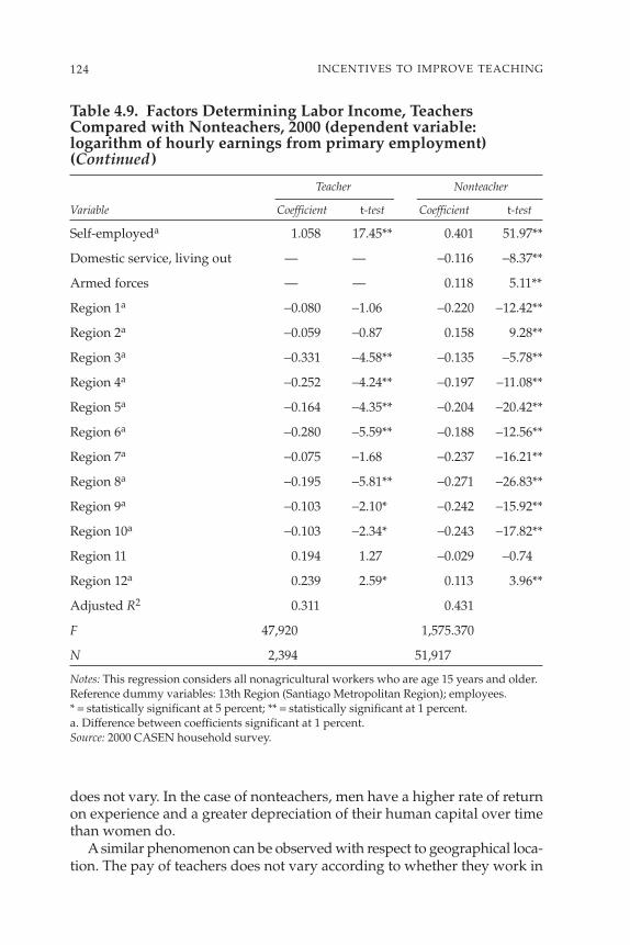
124 INCENTIVES TO IMPROVE TEACHING
Self-employeda 1.058 17.45** 0.401 51.97**
Domestic service, living out — — −0.116 −8.37**
Armed forces — — 0.118 5.11**
Region 1a −0.080 −1.06 −0.220 −12.42**
Region 2a −0.059 −0.87 0.158 9.28**
Region 3a −0.331 −4.58** −0.135 −5.78**
Region 4a −0.252 −4.24** −0.197 −11.08**
Region 5a −0.164 −4.35** −0.204 −20.42**
Region 6a −0.280 −5.59** −0.188 −12.56**
Region 7a −0.075 −1.68 −0.237 −16.21**
Region 8a −0.195 −5.81** −0.271 −26.83**
Region 9a −0.103 −2.10* −0.242 −15.92**
Region 10a −0.103 −2.34* −0.243 −17.82**
Region 11 0.194 1.27 −0.029 −0.74
Region 12a 0.239 2.59* 0.113 3.96**
Adjusted R2 0.311 0.431
F 47,920 1,575.370
N 2,394 51,917
Notes: This regression considers all nonagricultural workers who are age 15 years and older.Reference dummy variables: 13th Region (Santiago Metropolitan Region); employees. * = statistically significant at 5 percent; ** = statistically significant at 1 percent.a. Difference between coefficients significant at 1 percent.Source: 2000 CASEN household survey.
Table 4.9. Factors Determining Labor Income, Teachers Compared with Nonteachers, 2000 (dependent variable: logarithm of hourly earnings from primary employment) (Continued)
Teacher Nonteacher
Variable Coefficient t-test Coefficient t-test
does not vary. In the case of nonteachers, men have a higher rate of returnon experience and a greater depreciation of their human capital over timethan women do.
A similar phenomenon can be observed with respect to geographical loca-tion. The pay of teachers does not vary according to whether they work in

125TEACHERS’ SALARY STRUCTURE AND INCENTIVES IN CHILE
urban or rural areas or in other administrative regions within the country.29
This improved degree of earning equality by gender and location amongteachers reflects how teachers’ pay is calculated, especially for those workingin the municipal school sector, as set out in the Teachers’ Statute.
An interesting point to note is that—when we run a single equation inwhich the returns are assumed to be the same for both groups—we obtaina dummy variable for being a teacher that is equal to 0.028 (for 1998),which is statistically significant at a 10 percent level, and another variableequal to 0.044 (for 2000), which is statistically significant at a 5 percentlevel. The results imply that, on average, teachers earn salaries similar toworkers with the same characteristics, although this difference is slightlymore positive for 2000.
However, if we allow the returns to be different for teachers and non-teachers, the analysis shows that the earnings profile for teachers is differentfrom the earnings of other workers. Although gender and region have sta-tistically significant effects on the earnings of nonteachers, those factors donot affect teachers’ pay. In addition, although the return on years of school-ing and on having a professional degree is statistically significant, it is less sofor teachers than for nonteachers. However, the constant term is higher forteachers, so the earnings profile for teachers starts above the profile for non-teachers but is flatter.30
To better understand the results obtained from estimating equation 4.1,we first broke down earning differentials between teachers and nonteach-ers. Second, we simulated earnings that were predicted by the estimatedmodel, distinguishing between men and women.
Breakdown of Earning Differentials between Teachers and Nonteachers
The exercise to break down earning differentials enabled us to determinethe extent to which earning differentials reflect differences in individualcharacteristics and the returns on those characteristics. For this purpose,we applied the Oaxaca (1973) decomposition formula. This formula can bewritten as
4 2.( ) ( ) − ( ) = −( ) + −( )Ln W hr Ln W hr X X XT N N T N T N Tβ β β
29. The country is divided into 13 administrative regions. Santiago, the capital city, is inthe Metropolitan Region.
30. These results do not change when the income equation takes into account only teach-ers (937) and nonteachers (2,696) with 17 or more years of schooling. The constant termremains higher for teachers than for other workers, but the return on years of schooling is notstatistically significant for teachers. Only the variable of having a professional degree signif-icantly affects teachers’ hourly income.
In other words, the difference predicted by the regression model in the logof hourly earnings between teachers and nonteachers can be broken downin two parts. One part is explained by the differences in individual charac-teristics between the two groups (years of schooling, experience, and soforth) weighted by the coefficients estimated for nonteachers in the incomeequation. The other part is explained by the differences in rates of return oneach of those characteristics between teachers and other workers.
Equation 4.2 can be broken down still further. The first term on the right-hand side can be separated into (a) factors relating to personal characteris-tics (P) such as employee, self-employed, or owner and (b) characteristics ofthe job (J) such as geographic location (that is, urban or rural). The resultsfrom carrying out this exercise are shown in equation 4.3:
The results show that the difference in the log of main-job hourly earningsbetween teachers and nonteachers favors teachers in both years (0.70 for1998 and 0.54 for 2000). This finding is explained by differences in the per-sonal characteristics of teachers such as years of schooling, holding a pro-fessional title, and so forth (0.81 for 1998 and 0.64 for 2000). Moreover,characteristics that can be attributed to the job rather than to the teachersthemselves (mainly occupational category) reduce this differential (−0.14).
The final term in the equation shows the fraction of the earnings differ-ential between teachers and nonteachers that are attributed to differencesin returns on personal characteristics. The result obtained (+0.03 in 1998and +0.04 in 2000) indicates that teachers receive a little bit more in returnfor their personal characteristics than nonteachers do.
This result occurs despite the fact that the return on education and expe-rience for teachers is lower than for other workers. Several elements com-bine to explain this situation. First is the fact that teachers start with highersalaries than other workers with similar characteristics.31 Second, salariesare similar for male and females teachers; this fact does not occur for salariesof other men and women in the labor market. In most occupations, womenreceive lower yields than men for their human capital. Third, unlike otherworkers, teachers do not earn less because they are single or work outsidethe Metropolitan Region. All those elements tend to offset the differencesbetween teachers and nonteachers when it comes to their returns on educa-tion and experience.
4 3.( ) ( ) − ( ) = −( )+ −( ) + −( )
Ln W hr Ln W hr X X
X X X
T N Np
Tp
Np
NJ
TJ
NJ
T N T
β
β β β
126 INCENTIVES TO IMPROVE TEACHING
31. This element is reflected in the constant term of the estimated model (see tables 4.7and 4.8).

Earning Differentials between Teachers and Nonteachers
The above results show that researchers must pay attention to differencesbetween men and women when we compare salaries of teachers and non-teachers. In this section, we explore the issue in more detail.
Figure 4.3 presents the differences obtained from the estimated equa-tion 4.1 in the log of main-job hourly earnings between teachers and non-teachers in 1998, for different levels of schooling and potential experience.Figure 4.3a presents the case of women and figure 4.3b that of men. Theestimates for 2000 is similar, although a small improvement occurs formale teachers.32
Female teachers with up to 16 years of schooling earn more than femalenonteachers for any level of experience. Only female teachers with morethan 17 years of schooling (with graduate studies) earn less than non-teachers. Of female teachers, 64.9 percent receive higher salaries than non-teachers do.
For male teachers, the situation is different. Only male teachers with 13years of schooling or less earn more than male nonteachers for any level ofexperience. With 14 or 15 years of schooling, they earn more than non-teachers only at the beginning of their working lives and then again aftermany years of experience. Male teachers with 16 or more years of school-ing earn less than nonteachers, given their education and experience. Only21.8 percent of male teachers receive higher salaries than nonteachers.
The differences found between men and women reflect the fact that, incontrast with what happens in the rest of the Chilean labor market, nowage discrimination occurs against women in the teaching profession.33
Incentives Embedded within Teachers’ Salary Structure
The previous section shows that the basic issue with respect to teachers’salaries in Chile is not their average level but the fact that salaries are excep-tionally uniform from one teacher to another. Our analysis reveals thatthis characteristic occurs because the returns on education and experienceare low, comparably speaking, for teachers.
127TEACHERS’ SALARY STRUCTURE AND INCENTIVES IN CHILE
32. The figures start at 8 years of education because some teachers are trained at normalschools with that level of education (see appendix 4.F).
33. This lack of discrimination can be better explained by the regulated pay scalesintended to ensure teachers’ pay equity than by the fact that the teaching profession is afemale-dominated occupation. Verdugo and Schneider (1994) examined earning differentialsbetween male and female teachers in the United States and found that the latter appear toexperience wage discrimination. The cost associated with being a woman is approximately5 percent of the average annual salary.

128 INCENTIVES TO IMPROVE TEACHING
89
101112131415161718192021
0 5 10 15 20 25 30 35 40 45 50Potential experience
Year
s of
sch
oolin
g
Teachers Wages < Nonteachers Wages(35.1% of teachers)
Teacher Wages ≥ Nonteachers Wages(64.9% of teachers)
Source: Authors’ calculations.
Figure 4.3a. Salary Differentials between Female Teachersand Nonteachers, 1998
Teachers Wages < Nonteachers Wages (78.2% of teachers)
Teacher Wages ≥ Nonteachers Wages(21.8% of teachers)
89
101112131415161718192021
0 5 10 15 20 25 30 35 40 45 50Potential experience
Year
s of
sch
oolin
g
Source: Authors’ calculations.
Figure 4.3b. Salary Differentials between Male Teachersand Nonteachers, 1998

Permitting a more flexible salary structure in which part of salariesdepends on teachers’ performance could decompress the salary structurefor teachers, allowing the government to pay better salaries to those whoperform better. Since 1996, Chile has had a mechanism, the SNED, whichmakes it possible to adjust the salaries of teachers to their performance inthe country’s publicly financed schools. This mechanism is a collectiveincentive open to all schools receiving government funding (that is,municipal and subsidized private schools).
The amount of money that teachers receive under the SNED, however,is the lowest of all the monetary incentives to which they can aspire. In fig-ure 4.4, we compare the average increase received by a teacher at a schoolwith a SNED award (23,000 Chilean pesos per month) with other availableincentives. In each case, we compare the maximum amounts of theallowances.
An interesting point to note is that, since 2002, two incentives have beenprovided to reward individual excellence among teachers: (a) an individ-ual allowance for teaching excellence and (b) an allowance for the teach-ers’ tutor program. In the case of the former, teachers must voluntarilyparticipate in having their files evaluated and must take a test of theirknowledge. Teachers obtaining the reward receive double the SNEDaward, that is, 46,000 pesos per month.34 Moreover, if the teacher is willingto participate in peer training, then he or she may receive an additional50,000 pesos per month.
Despite the recent appearance of those collective and individual perfor-mance incentives, the most important incentive offered to teachers is senior-ity: a teacher with 30 years of service receives an additional 275,000 pesosper month. The second most significant incentive is the pursuit of furtherprofessional training, in which case teachers’ monthly income may increaseby 110,000 pesos. If teachers work in difficult conditions, for example, ingeographic isolation or with poor students, marginal students, or both,then they receive an additional 80,000 pesos per month. Finally, if teachersleave the classroom to assume management or technical positions, theirmonthly income rises 55,000 pesos.
Table 4.10 demonstrates the importance of different wage incentives tothe average teacher working in the municipal sector. The table presents therelative importance of the different kinds of bonuses in 2003. In each case,except for the basic national wage, the allowance has been calculated asthe total amount of money allocated to the municipal sector for this pur-pose, divided by the total number of municipal teachers.35 The first note-worthy element here is the complex salary structure.
129TEACHERS’ SALARY STRUCTURE AND INCENTIVES IN CHILE
34. See appendix 4.A for more details on the amounts paid for this purpose—in particular,pedagogical excellence allowance and variable allowance for individual performance.
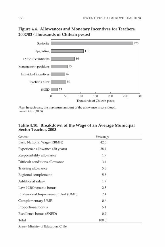
130 INCENTIVES TO IMPROVE TEACHING
Table 4.10. Breakdown of the Wage of an Average MunicipalSector Teacher, 2003
Concept Percentage
Basic National Wage (RBMN) 42.5
Experience allowance (20 years) 28.4
Responsibility allowance 1.7
Difficult conditions allowance 3.4
Training allowance 5.3
Regional complement 5.5
Additional salary 1.7
Law 19200 taxable bonus 2.5
Professional Improvement Unit (UMP) 2.4
Complementary UMP 0.6
Proportional bonus 5.1
Excellence bonus (SNED) 0.9
Total 100.0
Source: Ministry of Education, Chile.
Thousands of Chilean pesos
23
50
46
55
80
110
275
SNED
Teacher’s tutor
Individual incentives
Management positions
Difficult conditions
Upgrading
Seniority
Note: In each case, the maximum amount of the allowance is considered.Source: Cox (2003).
0 50 100 150 200 250 300
Figure 4.4. Allowances and Monetary Incentives for Teachers,2002/03 (Thousands of Chilean pesos)

One can conclude that—despite the inclusion of performance incentives—traditional incentives continue to be extremely important to Chilean teachers’salaries. Seniority is the main way of increasing income, which ultimatelymeans that loyalty rather than actual job performance is rewarded in theteaching profession. Undoubtedly, this situation has limited the SNED’sability to effectively change teachers’ behavior.
Nonetheless, some significant changes have occurred recently, andthose changes have boosted the importance of variable, performance-linked salaries. Specifically, in 2003 during the last round of collective bar-gaining between the teachers’ association and the Ministry of Education,both parties agreed that salary increases would be variable and assignedthrough the SNED, an agreement that became Law 19933 and came intoeffect on February 12, 2004. In the next section, we describe this system inmore detail, along with the changes that will take place in coming years.This system also established a new individual incentive for rewardingthose with distinguished or competent skills under individual evaluationprocesses currently under way. (In contrast to the teaching excellencebonus, this evaluation is compulsory.) Notwithstanding, the only evalu-ation under way that links teachers’ salaries to students’ performance isthe SNED.
Effect of the SNED on Schools’ Academic Achievement: A Preliminary Evaluation
In this section,36 we first describe the SNED and then estimate its effect onschools’ academic achievement after the first four applications. This study ispreliminary, so the results presented here are still of an exploratory nature.
The SNED rewards teachers for their performance and seeks to improvetheir motivation. The schools that perform with excellence are chosen every2 years and receive an excellence bonus as an incentive. The bonus isdefined on a per student basis, so the amount each school receives dependson the number of students in attendance. Schools representing up to 25 per-cent of each region’s enrollment receive awards. One requirement is that90 percent of the amounts assigned must go directly to the school’s teach-ers, in proportion to their hours of employment; each school decides the
131TEACHERS’ SALARY STRUCTURE AND INCENTIVES IN CHILE
35. For instance, in the case of the SNED, approximately 27 percent of municipal teach-ers receive the award, but the figure (0.9 percent) in table 4.10 assumes that the total amountof excellence bonus allocated to municipal teachers is divided by the total number of munic-ipal teachers.
36. This section is based on Mizala, Romaguera, and Henríquez (2004). More details onthe SNED can be found in Mizala and Romaguera (2002).

distribution of the remaining 10 percent. The SNED has been applied fourtimes since 1996.37
On average, 20 percent of the schools and approximately 27 percent ofthe teachers received awards in different applications of the SNED. Thosefigures varied for each year (see table 4.11).38 The subsidy for excellencethat teachers received during 2002/03 was 279,000 Chilean pesos per year(US$439.40),39 slightly more than the 219,000 pesos they obtained in 1996when the system began. This figure currently amounts to 87 percent of themonthly starting salary for teachers and a little more than an additional halfsalary per year for a teacher working 36.3 hours per week. The SNED’sexcellence award implies a salary increase that ranges from 7.2 percent peryear among those receiving the teachers’ starting salary to 4.7 percent forthose earning an average salary for 36.3 hours per week. As already men-tioned, the additional income involved in the award is relatively low, whichcould seriously limit the effect of this policy on teachers’ behavior.
The changes covered by the law that was recently approved by Congresssignificantly increase the excellence subsidy paid per student and, there-fore, the average annual amount that teachers at prize-winning schools willreceive. Table 4.12 shows that the amount of the per student excellenceaward will rise 91 percent between 2004 and 2006, which means that teach-
132 INCENTIVES TO IMPROVE TEACHING
Table 4.11. SNED: Beneficiaries and Resources
1996/97 1998/99 2000/01 2002/03
Schools receiving awards 2,274 1,832 1,699 1,863
Percentage of schools receiving — 20.2 18.4 19.7awards
Teachers receiving awards 30,600 31,400 32,600 34,400
Percentage of teachers receiving — 27.3 27.7 27.7awards
Excellence subsidy per teacher 345.2 364.4 428.3 439.4(annual in 2001 US$)
Total SNED budget (in thousands 10,563 11,442 13,963 15,115of 2001 US$)
Note: The average exchange rate in 2001 was 634.9 Chilean pesos per U.S. dollar.Source: Ministry of Education, Chile.
37. In March 2004, the results from the fifth application SNED were published.38. For the total number of SNED applications, 50.9 percent of schools have never received
the award; 27.7 percent have won once, 13.7 percent twice, 5.8 percent three times, and just1.8 percent every time the SNED has been applied.
39. This amount is paid quarterly during a period of 2 years.

ers working in a SNED prize-winning school will receive about doublewhat they are receiving today.
At the same time, the law establishes that more schools and teachers willreceive awards because the share of regional enrollment covered by awardswill rise from 25 percent to 35 percent in 2006. Schools ranking in the upper25 percent of regional enrollment will receive 100 percent of the excellencesubsidy, while those in the next 10 percent will receive 60 percent of theexcellence subsidy.
The Effect of the SNED on Schools’ Academic Achievement
We had to deal with several methodological challenges before we couldevaluate the SNED’s effect. In the first place, by definition, all Chileanschools receiving state funding participate in the SNED, with no need tocompete formally, so no schools are available for a comparison group.Because of this situation, the only feasible design to evaluate the SNED’seffect in schools is a reflexive comparison.40
Second, we had to deal with a problem of endogeneity. We are trying toevaluate the SNED’s effect on schools’ academic achievement, but theschool’s performance on students’ standardized tests is precisely one of themain variables considered (with a weight of 65 percent—factors “Effective-ness” and “Improvement”) to calculate the SNED index, which ranksschools and selects those to receive awards.
133TEACHERS’ SALARY STRUCTURE AND INCENTIVES IN CHILE
Table 4.12. Trends in SNED Award Amounts (2001 U.S. dollars)
January January January Years 1996/97 1998/99 2000/01 2002/03 2004 2005 2006
Per student 1.27 1.39 1.60 1.63 1.79 2.77 3.42excellence subsidy
Average 345.20 364.40 428.30 439.40 512.80a 827.00a —annual amount for award-winning teachers
Note: The average exchange rate in 2001 was 634.9 Chilean pesos per U.S. dollar.a. Based on the number of teachers who will receive the SNED award during 2004/05. — = not available.Source: Ministry of Education, Chile.
40. In a reflexive comparison, the counterfactual state is given by the pre-program par-ticipation of participants (prefactual scenario). See Duflo (2002), Grossman (1994), Heckmanand Smith (1995), Ravallion (2001), and Regalia (1999).
At the international level, some studies have estimated the effect ofaccountability systems that are associated with incentive payments. Amongthem are Ladd (1999), Lavy (2002a, 2002b), and Henry and Rubinstein(2002). In Chile’s case, virtually no studies have evaluated the SNED’s effecton educational achievement. One exception is Contreras and others (2003),which analyzes the effect of the 1998/99 SNED application on schools’ edu-cational achievement, measured by the results obtained on the 2000 Sistemade Medición de la Calidad de la Educación (Education Quality Measure-ment System, or SIMCE) test. Using ordinary least square (OLS) estimatesand the matching propensity score method, they found that the SNEDincreased SIMCE scores by an amount that fluctuates from 4 to 18 points.However, Contreras and others (2003) did not correct for the problem ofendogeneity when estimating the SNED’s effect on schools’ academic out-put, so their results might be biased.
The problem of endogeneity is common when evaluating programs,and the literature reveals different attempts to resolve it. The most widelyused solution is the use of instrumental variables, which would mean, inthe case of the SNED, finding a variable highly correlated to winning theSNED award but not highly correlated with the school’s ability to obtainhigh scores on the SIMCE test. Finding the right instrumental variable isnot easy, and the use of variables that do not totally satisfy the require-ments leads to biases greater than those already existing.41
An alternative strategy for dealing with the problem of endogeneity is toestimate a model with fixed effects for each school, which makes it possibleto model its heterogeneity. Schools’ fixed effects can vary or not over time.In this case, we consider only schools’ fixed effects that do not change overtime. Therefore, there may still be biases caused by changes that are notcontrolled by the fixed effects.
In this study, we apply a general fixed-effect model that makes it pos-sible for the (SNED) policy effects and biases to vary over time. Traditionalfixed-effect models, which assume coefficients that are constant over timeand that assume a bias caused by the also-constant, nonrandom selectionof schools, can be nested in this more general model.
In the case of the SNED, one could assume that the treatment effectsare the same every year because the methodology that has been applied (atleast in the past three applications) and even the resources that have beenallocated have not changed significantly. In other words, the same pro-
134 INCENTIVES TO IMPROVE TEACHING
41. In the case of the SNED, it is natural to think of the other SNED index factors as instru-mental variables. This strategy works only if one seeks to evaluate the effect of the SNED ofone period on achievements of the next period. However, when one considers an analysis ofseveral periods, it becomes difficult to use the other SNED indicators because they are allrelative to each application and are not comparable (in value) from one period to another.
gram has been applied every 2 years since 1996. However, schools’ aware-ness of the SNED, its reception, and its level of acceptance may eventu-ally change over time, and that change would make it possible for adifferent effect to occur for each period.
The traditional, fixed-effect model assumes a constant bias because ofthe nonrandom selection of schools, a selection that is based on fixed char-acteristics. This constant bias tends to be true in the SNED’s case becauseschools that perform well tend to always receive rewards, just as otherschools that have never received awards will probably not receive themin the future. Moreover, criteria for awards have remained stable overtime. Therefore, it would seem that the assumption holds true in theSNED’s case. Nonetheless, as in the previous case, it might be interestingto consider a model that relaxes this restriction, assuming instead that thecriteria for allocating the awards change between applications. The advan-tage of using this kind of “relaxed” model is that the different SNED appli-cations can be considered in a single regression, thereby producing moreprecise and robust estimates than other methods such as the difference-in-difference method.
The Model
We consider the following type of model for the production function42 aswe evaluate the SNED’s effect on schools’ educational achievement (effec-tiveness measured by SIMCE scores):
In this model, Est represents effectiveness of school s over time t, Xst rep-resents characteristics of school s over time t, SNEDs,t−1 represents theSNED award (dummy variable) of school s over time t − 1, Cs representsunobservable fixed characteristics of school s, and Fs represents observablefixed characteristics of school s.
This model assumes that the unobserved fixed effect (Cs) of school sdoes not correlate with the error term (εst), although it may correlate withother characteristics of the school, whether fixed (Fs) or variable (Xst). Ourmain interest is in the relationship between unobservable characteristics(Cs) and the SNED selection variable (SNEDst). Note that the model con-siders the effect of the SNED award from the previous period because,when the next period starts, the granting of the award has been completed.
4 4 1. ,( ) = ′ + ′ + ′ +−E X SNED Cst t st t s t t s stα β γ ε
135TEACHERS’ SALARY STRUCTURE AND INCENTIVES IN CHILE
42. Jakubson (1991) uses this model to estimate unions’ effects on salaries. Meanwhile,Tokman (2002) uses a similar model to analyze the effects of the P900 program on schools’educational performance.

If we assume that Cs can be correlated with the SNEDst variable, wecan model the SNED’s effect on unobservable school characteristics asfollows:
where t, as 0, 1, 2, refers to the 1996/97, 1998/99, and 2000/01 SNED appli-cation periods. Note that the coefficients λj may vary with the period,thus incorporating the possibility that schools’ unobservable characteris-tics affect the award differently in each period, thereby incorporating abias in estimated effects that may vary over time.
Substituting the expression for Cs from equation 4.5 in equation 4.4, weget the following specification:
in which γ and λ together determine the bias.Equation 4.6 is a restricted version of the following more general model:
where
Depending on our assumptions, we find different specifications of matrixII and, therefore, different specifications of equation 4.7. Consider two pos-sibilities in particular. First, if we consider that the SNED effect, the effectof unobservable characteristics, and the effect of biases change over time,then the coefficients βj, γj, and λj are different for each period, yielding thefollowing specification for Π, which corresponds to equation 4.3:
4 8
1 1 1
2 1
3 1
1 2
2 2 2
3 2
1 3
2 3
3 3 3
. ˜( ) =
+
+
+
Π
β γ λ
γ λ
γ λ
γ λ
β γ λ
γ λ
γ λ
γ λ
β γ λ
E
E
E
E
X
F X
F X
F X
SNED
SNED
SNED
SNED
and e
e
e
e
s
s
s
s
s
s s
s s
s s
s
s
s
s
s
s
s
s
=
=
=
=
1
2
3
1
2
3
0
1
2
1
2
3
, , .
4 7.( ) = + +E X SNED es s s sΦ Π
4 6 1. ,( ) = ′ + ′
+ ′ ′ + + +( )−E X SNED
SNED F
st t st t s t
t s s t s st
α β
γ λ δ γξ ε
4 5 1 0 2 1 3 2.( ) = + +
+ = ′ +
C SNED SNED SNED
SNED
s s s s
st s st
λ λ λ
ξ λ ξ
136 INCENTIVES TO IMPROVE TEACHING
Second, if we consider that the SNED effect (βj) is the same for each period,but that the effect of unobservable characteristics and biases changes overtime, then the coefficients γj and λj are different for each period, yieldingthe following specification for Π:
To evaluate the admissibility of those different restrictions, we can useminimum distance estimators (Chamberlain 1982, 1990) and can estimateparameters using generalized least squares with (nonlinear) restrictions.
As mentioned, the models estimated use effectiveness as a dependentvariable. This variable is defined as a valid average43 of each school’s scoreon the SIMCE tests closest to the year being considered.44 The explanatoryvariable is whether or not the school won a SNED award. The control vari-ables are school characteristics such as socioeconomic level, which is mea-sured using an index that combines parental income, household income,and the Junta Nacional de Auxilio Escolar y Becas (National School Supportand Scholarship Board, or JUNAEB) vulnerability index; size, which ismeasured by enrollment; full or partial school day (jornada escolar completa);participation in other programs such as the P900; educational level (pri-mary or secondary); location (urban or rural); students’ gender; regionwhere the school is located; type (municipal or private subsidized); andeffectiveness in previous years (we used 1996 as our base year).45
The variables are available for each school in a panel-type data setwhere the observations correspond to schools that have participated inall SNED applications since 1998 and have taken the SIMCE tests, so thoseschools have data for the effectiveness variable.
One important issue to consider is that the SNED may not be an incen-tive for all schools, although the system does allow for some turnover in
4 9
1 1
2 1
3 1
1 2
2 2
3 2
1 3
2 3
3 3
. ˜( ) =
+
+
+
Π
β γ λ
γ λ
γ λ
γ λ
β γ λ
γ λ
γ λ
γ λ
β γ λ
137TEACHERS’ SALARY STRUCTURE AND INCENTIVES IN CHILE
43. A valid average is defined as the average of scores for the tests to which the schoolmust submit, depending on the school type.
44. It is important to note that the effectiveness variable included in the SNED index fortime t and the effectiveness variable used in the model (Est) are not the same, although oneof the tests is included in both indicators in each period.
45. Finally, given the possibility that “noise” in the results of standardized tests maylimit using the tests in school rankings and in accountability systems (Chay, McEwan, andUrquiola 2003; Kane and Staiger 2002), we analyze to what degree the effectiveness variablemay present more variability in smaller schools. However, the effectiveness variable is simi-lar in every decile of school size (see appendix 4.H). This similarity may reflect the fact thatthe effectiveness variable includes language and mathematics tests given to different grades(4th, 8th, and 10th) in different years.
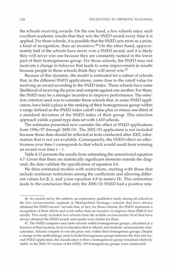
the schools receiving awards. On the one hand, a few schools enjoy suchexcellent academic results that they win the SNED award every time it isapplied. For those schools, it is possible that the SNED acts more as a prize,a kind of recognition, than an incentive.46 On the other hand, approxi-mately half of the schools have never won a SNED award, and it is likelythey will never win one because they are constantly ranked in the lowerpart of their homogeneous group. For those schools, the SNED may notmotivate a change in behavior that leads to some improvement in resultsbecause people in those schools think they will never win.47
Because of this dynamic, the model is estimated for a subset of schoolsthat, in the different SNED applications, come close to the cutoff value forreceiving an award according to the SNED index. Those schools have somelikelihood of receiving the prize and compete against one another. For them,the SNED may be a stronger incentive to improve performance. The selec-tion criterion used was to consider those schools that, in some SNED appli-cation, have held a place in the ranking of their homogeneous group withina range defined as the SNED index cutoff value plus or minus one-third ofa standard deviation of the SNED index of their group. This selectionapproach yields a panel-type data set with 1,610 schools.
The estimates presented next consider the effect of SNED applicationsfrom 1996/97 through 2000/01. The 2002/03 application is not includedbecause those data should be reflected in tests conducted after 2002, infor-mation that is not yet available. Consequently, the SNED effect on effec-tiveness over time t corresponds to that which would result from winningan award over time t − 1.
Table 4.13 presents the results from estimating the unrestricted equation4.7. Given that there are statistically significant elements outside the diag-onal, the data validate the specification of equation 4.6.
We then estimated models with restrictions, starting with those thatinclude nonlinear restrictions among the coefficients and allowing differ-ent values for β, λ, and γ (see equation 4.8 in matrix Π). This estimationleads to the conclusion that only the 2000/01 SNED had a positive rela-
138 INCENTIVES TO IMPROVE TEACHING
46. As carried out by the authors, an exploratory qualitative study among all schools inthe low socioeconomic segment in Metropolitan Santiago—schools that have alwaysobtained the SNED award—reveals that, in fact, for those schools, the SNED represents arecognition of their efforts and work rather than an incentive to improve their SIMCE testresults. This study included two schools from the middle socioeconomic level that havealways obtained the SNED award, and results were similar for them.
47. The SNED compares and ranks schools within homogeneous groups, calculated as afunction of their location, level of education that is offered, and students’ socioeconomic char-acteristics. Schools compete to win the prize only within their homogenous groups. Despitea change in the methodology used to build homogeneous groups between the first and sec-ond SNED application, the classification within a homogeneous group remained relativelystable. In the 2002/03 version of the SNED, 109 homogeneous groups were constructed.
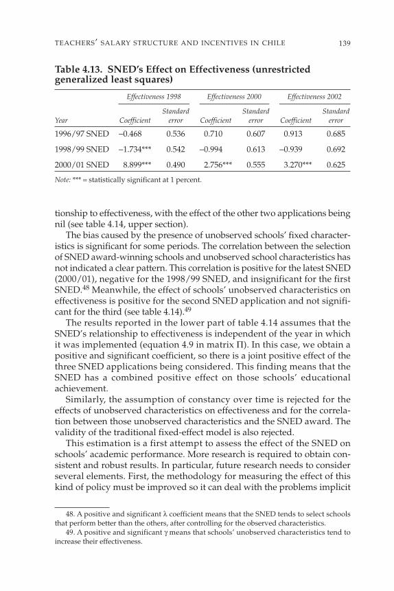
tionship to effectiveness, with the effect of the other two applications beingnil (see table 4.14, upper section).
The bias caused by the presence of unobserved schools’ fixed character-istics is significant for some periods. The correlation between the selectionof SNED award-winning schools and unobserved school characteristics hasnot indicated a clear pattern. This correlation is positive for the latest SNED(2000/01), negative for the 1998/99 SNED, and insignificant for the firstSNED.48 Meanwhile, the effect of schools’ unobserved characteristics oneffectiveness is positive for the second SNED application and not signifi-cant for the third (see table 4.14).49
The results reported in the lower part of table 4.14 assumes that theSNED’s relationship to effectiveness is independent of the year in whichit was implemented (equation 4.9 in matrix Π). In this case, we obtain apositive and significant coefficient, so there is a joint positive effect of thethree SNED applications being considered. This finding means that theSNED has a combined positive effect on those schools’ educationalachievement.
Similarly, the assumption of constancy over time is rejected for theeffects of unobserved characteristics on effectiveness and for the correla-tion between those unobserved characteristics and the SNED award. Thevalidity of the traditional fixed-effect model is also rejected.
This estimation is a first attempt to assess the effect of the SNED onschools’ academic performance. More research is required to obtain con-sistent and robust results. In particular, future research needs to considerseveral elements. First, the methodology for measuring the effect of thiskind of policy must be improved so it can deal with the problems implicit
139TEACHERS’ SALARY STRUCTURE AND INCENTIVES IN CHILE
Table 4.13. SNED’s Effect on Effectiveness (unrestricted generalized least squares)
Effectiveness 1998 Effectiveness 2000 Effectiveness 2002
Standard Standard Standard Year Coefficient error Coefficient error Coefficient error
1996/97 SNED −0.468 0.536 0.710 0.607 0.913 0.685
1998/99 SNED −1.734*** 0.542 −0.994 0.613 −0.939 0.692
2000/01 SNED 8.899*** 0.490 2.756*** 0.555 3.270*** 0.625
Note: *** = statistically significant at 1 percent.
48. A positive and significant λ coefficient means that the SNED tends to select schoolsthat perform better than the others, after controlling for the observed characteristics.
49. A positive and significant γ means that schools’ unobserved characteristics tend toincrease their effectiveness.
140IN
CE
NT
IVE
ST
OIM
PR
OV
ET
EA
CH
ING
Table 4.14. SNED Relationship to Effectiveness (N = 1,610 schools)
β1 β2 β3 λ1 λ2 λ3 γ2 γ3
Coefficient 0.0727 0.2652 2.5883 −0.8189 −1.6101 8.9477 0.2753 0.0106
Standard error 1.9328 0.5576 3.0571 1.9525 0.5221 0.4763 0.0586 0.3377
Significance * *** *** ***
χ2 (1) 7.56
Coefficient 0.7576 −1.3708 −1.7387 8.7119 0.2235 0.0752
Standard error 0.5260 0.7293 0.5149 0.4758 0.0582 0.0900
Significance ** ** *** *** ***
χ2 (3) 14.14
Note: * = statistically significant at 10 percent; ** = statistically significant at 5 percent; *** = statistically significant at 1 percent.
Nonlinear restrictionson coefficients
Constant SNEDcoefficient: Singleimpact of the program

in the lack of a control group and endogeneity. Second, data from the mostrecent SNED application must be included because obtaining reliableresults requires lengthy time series, particularly given that the SNED wasnot at first widely publicized among schools. Third, key evaluations willbe those that measure the SNED’s effects after the amounts allocated risein 2005 and again in 2006, when SNED coverage will increase to 35 percentof each region’s enrollment. This increment will be important becausetoday, as mentioned, the SNED offers only a modest monetary incentive towhich teachers can aspire.
Evaluating Performance and Incentives: Teachers’ and Principals’ Perceptions
Despite the fact that, when compared with other monetary incentives todate, the SNED is not notably significant, it has affected teachers’ attitudes.In fact, teachers seem more open today to performance evaluations andthe associated incentive payments. This apparent openness explains to alarge degree why the teachers’ association agreed to increase the variableportion of performance-linked salaries. Likewise, the experience with theSNED likely helped in reaching the agreement in 2000 in which individualperformance evaluations were accepted as a criterion for teaching careers.
Several surveys of teachers reveal this change in teachers’ traditionalresistance to evaluation systems. A first survey was done of a random sam-ple of Greater Santiago teachers to find out what they thought of the edu-cation system, and it included some questions about the SNED.50 In termsof their acceptance of performance evaluations and awards, responseswere positive. There was a high degree of consensus:
• Among teachers, 74.7 percent agreed or strongly agreed with the state-ment that the Ministry of Education should apply a performance eval-uating mechanism to subsidized private and public schools.
• Also among teachers, 87.6 percent agreed or strongly agreed with thestatement that it is important to recognize schools that perform betterthan others.
The sample group showed less agreement, although still more than half,with statements about the effect of the excellence award on the quality ofeducation and, therefore, on the link between salaries and evaluation:
141TEACHERS’ SALARY STRUCTURE AND INCENTIVES IN CHILE
50. Field work took place from November 26, 1998, to January 6, 1999, using surveyors.A random sample of 400 teachers in Greater Santiago was selected in two stages: (a) ran-domly selecting 50 award-winning schools and 50 schools that had never received the SNEDaward (42 municipal schools and 58 subsidized private schools) and (b) selecting four teach-ers per school at random. Of the selected sample of 400 teachers, 355 were actually inter-viewed (at 48 award-winning schools and at 50 with no award). See Mizala and others (2002).

• Among teachers, 55.6 percent agreed or strongly agreed with the state-ment that the excellence award for performance contributes to improv-ing the quality of education.
• Also among teachers, 58.3 percent agreed or strongly agreed with thestatement that the rise in teachers’ salaries should be linked to an evalu-ation of each person’s teaching.
Similarly, national surveys done by the Centro de Investigación yDesarrollo de la Educación (Center for Educational Research and Devel-opment, or CIDE) confirm the idea that teachers have greater acceptanceof performance evaluations. In the first survey (CIDE 2000), conducted in1999 with 1,053 teachers, 78.6 percent of teachers strongly agreed with anindividual evaluation of teaching performance. In the second survey, con-ducted in 2000 with 1,060 teachers, 70.3 percent said they strongly agreedwith individual evaluation of teaching performance. If replies are brokendown by type of school, the data reveal that 62 percent of teachers inmunicipal schools; 76.7 percent of teachers in private subsidized schools;and 84.8 percent of teachers in private, fee-paying schools agree with indi-vidual performance evaluations (Mella and Ostoic 2001). In the fourth sur-vey (CIDE 2003), of 1,154 teachers, 64 percent of those surveyed indicatedthat they agreed with implementing a teaching performance evaluationsystem that included incentives and sanctions. Again, the strongest agree-ment was among teachers in private, fee-paying schools (75 percent), fol-lowed by teachers in private subsidized schools (63 percent), and finallyby teachers in municipal schools (58 percent).
Moreover, a voluntary survey of principals of private subsidized andmunicipal schools in Chile, with responses from 3,338 out of 9,684 schools,found significant support for performance evaluations and performance-related monetary incentive payments.51 Moreover, most principals indi-cated that it is very useful to their work as principals to have a monetaryreward that is for teachers and is associated with school performance.
Figures 4.5, 4.6, and 4.7 present the results of the survey of principals,differencing according to the number of times the school has obtained theSNED award. Note that the answers tend to be more positive the moretimes the school has received the reward. Nonetheless, even principals ofschools that have never won the SNED show considerable acceptance ofperformance evaluations and payment of monetary incentives. Among
142 INCENTIVES TO IMPROVE TEACHING
51. Although this survey design with voluntary participation implies self-selection ofthose responding, no bias is apparent after comparing characteristics of schools that partici-pated with the characteristics of the total group of schools. Characteristics compared were theregion where the school is located, type (public or private), and level of education (primaryor secondary, adults, preschool, and so forth). Although the respondents’ sample is slightlyskewed in favor of schools that have received an award, this deviation is not worrisome(see appendix 4.J). More details can be found in Mizala and Romaguera (2004).

143TEACHERS’ SALARY STRUCTURE AND INCENTIVES IN CHILE
3.5
37.7
54.9
3.0
37.0
56.4
1.7
33.8
62.1
3.5
28.2
67.1
0.019.1
77.7
3.0
35.7
58.0
0
20
40
60
80
100
0 1 2 3 4 Total
Neither agree nor disagree Agree Strongly agree
Note: Other response options were “Strongly disagree” and “Disagree.” Source: Ministry of Education, Chile, 2003.
Perc
enta
ge o
f sch
ools
Number of times school won the SNED award
Figure 4.5. Responses of Principals: “I Agree or Strongly Agreewith MINEDUC Regularly Evaluating Schools Receiving StateSubsidies”
3.6
29.8
60.8
2.5
26.3
67.1
1.1
24.0
72.3
0.818.4
78.4
0.06.4
93.6
2.6
26.3
66.7
0
20
40
60
80
100
0 1 2 3 4 Total
Neither agree nor disagree Agree Strongly agree
Note: Other response options were “Strongly disagree” and “Disagree.” Source: Ministry of Education, Chile, 2003.
Perc
enta
ge o
f sch
ools
Number of times school won the SNED award
Figure 4.6. Responses of Principals: “I Agree or Strongly AgreeThat MINEDUC Should Provide Resources for RegularlyRewarding the Best Performing Schools”

principals, 78.5 percent consider this policy rather useful or very useful totheir work (see figure 4.7).
Conclusions
In this chapter, we have tried to look at teachers’ salaries in Chile and theincentives available to teachers from different perspectives. We have ana-lyzed the evolution and structure of teachers’ salaries, along with differ-entials that may exist when salaries are compared with those of otherprofessionals with similar characteristics.
An important point to emphasize is that most of the information avail-able refers to salaries paid in the municipal sector. No data are available onthe private sector because those salaries are negotiated at the individualschool level. The only information on the private sector is the startingsalary, plus some allowances that are valid for teachers in both public andprivate sectors.
This analysis makes it possible to conclude that—early in the 1990s—with the return of democracy, teachers’ salaries rose significantly in realterms, over and above the average wage of the economy and more thanthe average salary for professionals. This conclusion is also apparent in the
144 INCENTIVES TO IMPROVE TEACHING
15.2
19.2
59.3
13.8
18.0
63.7
11.9
17.9
66.2
8.2
20.4
68.6
4.37.4
86.2
13.5
18.4
63.1
0
20
40
60
80
100
0 1 2 3 4 Total
Useful Somewhat useful Useful
Note: Other response options were “Not useful at all” and “Not very useful.” Source: Ministry of Education, Chile, 2003.
Perc
enta
ge o
f sch
ools
Number of times school won the SNED award
Figure 4.7. Responses of Principals: “It Is ‘Very Useful,’‘Somewhat Useful,’ ‘Useful’ to Principal’s Work That There Is a Monetary Award to Teachers, Associated with SchoolPerformance, Financed and Designed to MINEDUC Standards”

starting salary for teachers, which has risen by more than the minimumwage within the economy. This rise in salaries may be one reason behindthe turnaround in the number of students going into training for the edu-cation field and the turnaround in their scores because both have risen sig-nificantly since 1998.
Given that comparing teachers’ and other workers’ salaries may not beappropriate because of the differences in human capital involved, we alsocarried out an econometric analysis that allowed us to compare similarworkers. This analysis showed that, on average, teachers’ earnings aresimilar to those of nonteachers with the same characteristics. However, theearnings profile for teachers is different from that of other workers becauseof how teachers’ salaries are calculated, especially for those in municipalschools. The return on schooling and on having a professional degree,though statistically significant, is lower for teachers than for other work-ers. The same is true with the return on experience.
Moreover, the income profile for teachers starts at a higher point thanfor other similar workers, but is flatter. Thus, teachers with less educationand experience earn more than they would in other sectors, whereas teach-ers with more education and experience earn less than similar workers inother occupations.
This salary structure suggests that teaching probably attracts peoplewith a preference for job stability and discourages the entry of people will-ing to take more risks. In this sense, even more educated teachers wouldnot necessarily be underpaid but, rather, could be accepting a compen-satory differential in exchange for job stability and security.
Similarly, we analyzed the incentives embedded in the salary structurefor teachers. We found that, despite the recent appearance of collective andindividual performance incentives, the main incentive to teachers contin-ues to be seniority and professional training. The SNED is the oldest ofthe performance evaluations that are linked to monetary incentives andthe only one that uses students’ academic achievement as the basic crite-rion. This incentive currently accounts for a small percentage of teachers’average monthly salary.
Preliminary estimates reveal that the SNED has had a positive effecton educational achievement in those schools that have been involved in itsdifferent applications and are close to (higher or lower than) the cutoffpoint between SNED award winners and losers. For this group of schools,it can be concluded that, on the one hand, the effect of an individual SNED(2000/01 being the most recent one considered) is significant. On the otherhand, there is a cumulative effect from the different SNED applicationson schools’ academic achievement.
Also, the SNED has had an effect on teachers’ attitudes. In fact, teach-ers today are more open to performance evaluation and the payment ofmonetary incentives linked to it. Principals consider evaluations and mon-etary incentives useful in carrying out their work.
145TEACHERS’ SALARY STRUCTURE AND INCENTIVES IN CHILE
This change in attitude explains to a large degree why the teachers’union recently accepted a proposal to boost the variable part of salarieslinked to performance. The experience with the SNED made it easier toreach agreement in 2000 about including voluntary accreditation of class-room skills, which is associated with a payment (pedagogical excellenceallowance). Similarly, in the recent round of collective bargaining in 2003,parties agreed to create an allowance to reward (a) those who qualified asdistinguished or competent in their compulsory individual performanceevaluation and (b) those who demonstrated their disciplinary and peda-gogical knowledge in a written test. The parties also agreed that part ofwage increases will be variable and will be allocated through the SNED.This agreement means that, from now until 2006, the monthly amountreceived by teachers working at a SNED-winning school will double. Atthe same time, the percentage of school enrollment receiving an award willrise from 25 percent to 35 percent, which means that more teachers andschools will receive this monetary incentive. It will be interesting to assessthe SNED’s effect on schools’ academic performance after these changeshave been implemented.
Such changes are very important because they represent significantprogress toward a more flexible salary structure in which part of salariesdepends on teachers’ performance. This change would decompress teach-ers’ salary structure, allowing the government to pay better salaries tothose who perform better. This wage policy would also encourage bettercandidates to enter and remain in the teaching profession.
146 INCENTIVES TO IMPROVE TEACHING

147
References
Ballou, D., and M. Podgursky. 1997. Teacher Pay and Teacher Quality. Kala-mazoo, Mich.: W. E. Upjohn Institute for Employment Research.
Belleï, C. 2001. “El talón de Aquiles de la reforma. Análisis sociológicode la política de los 90 hacia los docentes en Chile.” In S. Martinic andM. Pardo, eds., Economía política de las reformas educativas en AméricaLatina. Centro de Investigación y Desarrollo de la Educación–Programade Promoción de la Reforma Educativa en América Latina, Santiago.
Chamberlain G. 1982. “Multivariate Regression Models for Panel Data.”Journal of Economics 18: 5–46.
———. 1990. “Panel Data.” In Z. Griliches and M. Intriligator, eds., Hand-book of Econometrics (vol. 2). Amsterdam: Elsevier/North-Holland.
Chay, K. Y., P. J. McEwan, and M. Urquiola. 2003. “The Central Role ofNoise in Evaluating Interventions That Use Test Scores to RankSchools.” NBER Working Paper 10118. National Bureau of EconomicResearch, Cambridge, Mass.
CIDE (Centro de Investigación y Desarrollo de la Educación). 2000.“Encuesta nacional a los actores del sistema educativo 1999.” Centrode Investigación y Desarrollo de la Educación. Santiago. Processed.
———. 2003. “IV encuesta nacional a los actores del sistema educativo:Medición 2003.” Centro de Investigación y Desarrollo de la Educación,Santiago. Processed.
Contreras D., L. Flores, F. Lobato, and V. Macías. 2003. “Monetary Incentivesfor Teachers and School Performance: Evidence for Chile.” University ofChile, Department of Economics, Santiago. Processed.
Cowan, K., A. Micco, A. Mizala, C. Pages, and P. Romaguera. 2002. “Undiagnóstico del desempleo en Chile.” Inter-American DevelopmentBank, Washington, D.C. Processed.
Cox, C. 2003. “Las políticas educacionales de Chile en las últimas dosdécadas del siglo XX.” In C. Cox, ed., Políticas educacionales en el cambiode siglo. Santiago: Editorial Universitaria.
Duflo, E. 2002. “Empirical Methods.” Handout of courses MIT 14.771 andHarvard 2390b. Department of Economics, Massachusetts Institute ofTechnology, Boston. Processed.
ECLAC (Economic Commission for Latin America and the Caribbean).1999. Panorama social de América Latina 1998. Santiago.
Flyer, F., and S. Rosen. 1996. “Some Economies of Precollege Teaching.”In W. Becker and W. Baumol, eds., Assessing Educational Practices: TheContribution of Economics. Cambridge, Mass.: MIT Press.
González, P. 1998. Financiamiento de la educación en Chile. Santiago: Pro-grama de Promoción de la Reforma Educativa–United Nations Educa-tional, Scientific, and Cultural Organization.
González, P., A. Mizala, and P. Romaguera. 2001. “Recursos diferencia-dos para la educación subvencionada en Chile.” Centro de EconomíaAplicada, Departamento de Ingeniería Industrial, University of Chile,Santiago.
Grossman, J. B. 1994. “Evaluating Social Policies: Principles and U.S. Expe-rience.” World Bank Research Observer 9(2): 159–80.
Heckman, J., and J. Smith. 1995. “Assessing the Case for Social Experi-ments.” Journal of Economic Perspectives 9(2): 85–110.
Henry, G., and R. Rubinstein. 2002. “Paying for Grades: Impact of Merit-Based Financial Aid on Educational Quality.” Journal of Policy Analysisand Management 21(1): 93–109.
Jakubson, G. 1991. “Estimation and Testing of the Union Wage EffectUsing Panel Data.” Review of Economic Studies 58(5): 971–91.
Kane, T. J., and D. O. Staiger. 2002. “The Promises and Pitfalls of Impre-cise School Accountability Measures.” Journal of Economic Perspectives16(4): 91–114.
Komenan, A. G., and C. Grootaert. 1990. “Pay Differences betweenTeachers and Other Occupations: Some Empirical Evidence from Côted’Ivoire.” Economics of Education Review 9(3): 209–17.
Ladd, H. 1999. “The Dallas School Accountability and Incentive Program:An Evaluation of Its Impacts on Student Outcomes.” Economics of Edu-cation Review 18(1): 1–16.
148 INCENTIVES TO IMPROVE TEACHING

Lankford, H., and J. Wyckoff. 1997. “The Changing Structure of TeacherCompensation, 1970–94.” Economics of Education Review 16(4): 371–84.
Lavy, V. 2002a. “Evaluating the Effect of Teachers’ Group PerformanceIncentives on Pupil Achievement.” Journal of Political Economy 110(6):1286–317.
———. 2002b. “Paying for Performance: The Effect of Teachers’ FinancialIncentives on Students’ Scholastic Outcomes.” Hebrew University ofJerusalem, Department of Economics, Jerusalem. Processed.
Liang, X. 1999. “Teacher Pay in 12 Latin American Countries: How DoesTeacher Pay Compare to Other Professions, What Determines TeacherPay, and Who Are the Teachers?” Latin America and the CaribbeanRegion Human Development Department Paper 49. World Bank, Wash-ington, D.C.
López-Acevedo, G., and A. Salinas. 2000. “Teachers’ Salaries and Profes-sional Profile in Mexico.” Latin America and the Caribbean Region,World Bank, Washington, D.C. Processed.
Mella, O., and D. Ostoic. 2001. “II encuesta nacional a los actores del sis-tema educativo 2000.” Centro de Investigación y Desarrollo de la Edu-cación, Santiago. Processed.
Mincer, J. 1974. Schooling, Experience, and Earnings. New York: ColumbiaUniversity Press.
Mizala, A., and P. Romaguera. 2000a. “Remuneraciones al pizarrón.” Per-spectivas en Política, Economía y Gestión 4(1): 65–88.
———. 2000b. “School Performance and Choice: The Chilean Experience.”Journal of Human Resources 35(2): 392–417.
———. 2002. “Evaluación del desempeño e incentivos en la educaciónChilena.” Cuadernos de Economía 39(118): 353–94.
———. 2004. “Encuesta acerca del SNED a directores de establecimientossubvencionados.” Ministerio de Educación de Chile, Santiago. Processed.
Mizala, A., P. Romaguera, and M. Henríquez. 2004. “El SNED y el logroeducativo de los establecimientos educacionales en Chile.” Centro deEconomía Aplicada, Departamento de Ingeniería Industrial, Universityof Chile, Santiago. Processed.
149TEACHERS’ SALARY STRUCTURE AND INCENTIVES IN CHILE

Mizala, A., P. González, P. Romaguera, and A. Guzmán. 2002. “Chile: Larecuperación de la profesión docente es possible.” In J. C. Navarro, ed.,¿Quiénes son los maestros? Carreras e incentivos docentes en América Latina.Washington, D.C.: Inter-American Development Bank.
Mulcahy-Dunn, A., and G. Arcia. 1996. “Teachers’ Salaries and LivingStandards in Ecuador.” Center for International Development, ResearchTriangle Institute, Research Triangle Park, N.C. Processed.
Oaxaca, R. 1973. “Male-Female Wage Differentials in Urban Labor Mar-kets.” International Economic Review 14(3): 693–709.
Ormeño, A. 1996. “Evolución de la formación de profesores en Chile:Análisis por región, dependencia y nivel del sistema educacional.”Working Paper. Corporación de Promoción Universitaria, Santiago.
Piras, C., and W. Savedoff. 1998. “How Much Do Teachers Earn?” IDB Work-ing Paper 375. Inter-American Development Bank, Washington, D.C.
Psacharopoulos, G. 1987. “Are Teachers Overpaid? Some Evidence fromBrazil.” Teaching and Teacher Education 3: 315–18.
Psacharopoulos, G., J. Valenzuela, and M. Arends. 1996. “Teacher Salariesin Latin America: A Review.” Economics of Education Review 15(4): 401–6.
Ravallion, M. 2001. “The Mystery of the Vanishing Benefits: An Introduc-tion to Impact Evaluation.” World Bank Economic Review 15(1): 115–40.
Regalia, F. 1999. “Impact Evaluation Methods for Social Programs.”Poverty and Inequality Technical Note 2. Inter-American DevelopmentBank, Washington, D.C.
Tokman, A. 2002. “Evaluation of the P900 Program: A Targeted EducationProgram for Underperforming Schools.” Working Paper 170. BancoCentral de Chile, Santiago.
Vegas, E., W. Experton, and L. Pritchett. 1998. “Teachers in Argentina:Under- (Over-) worked? Under- (Over-) paid?” World Bank, Washington,D.C. Processed.
Verdugo, R., and J. Schneider. 1994. “Gender Inequality in Female-Dominated Occupation: The Earnings of Male and Female Teachers.”Economics of Education Review 13(3): 251–64.
Zymelman, M., and J. DeStephano. 1989. “Primary School Teachers’Salaries in Sub-Saharan Africa.” Discussion Paper 45. World Bank,Washington, D.C.
150 INCENTIVES TO IMPROVE TEACHING

5Educational Finance
Equalization, Spending, Teacher Quality, and
Student OutcomesThe Case of Brazil’s FUNDEF
Nora GordonUniversity of California at San Diego
and Emiliana VegasWorld Bank
Improving access to and quality of basic education for all children is aprimary concern of policymakers throughout the world. Expanding accessto basic education is still needed in many developing countries, and doingso while raising the quality of schooling has proved to be a challenge. Justwhich policy reforms are most effective at expanding access and improv-ing school quality is still an open question. The reform of the Fundo deManutenção e Desenvolvimento do Ensino Fundamental e de Valoriza-ção do Magistério (known as the Fund for the Maintenance and Develop-ment of Basic Education and Teacher Appreciation, or FUNDEF) is aneducational finance reform to improve access to and quality of basic edu-cation for all Brazilian children. The recent experience of FUNDEF can pro-vide useful evidence with respect to the effect that strategies to equalizeeducational finance have on access, quality, and equity of schooling.
The federal government of Brazil implemented FUNDEF in 1998. Itsmain objective was to promote greater equity in educational opportunitiesamong states and across the municipalities within states by guaranteeinga minimum per pupil expenditure in primary schools throughout thecountry and by partially equalizing per pupil funding within states. Before1998, education in Brazil was financed by a mandated share of subnationalgovernments’ revenue (both own source and revenue sharing), withoutconsidering the variation in enrollment or costs, which led to widespread
151

inequalities in per pupil financing among municipalities not only withinstates but also across states (Soares 1998).52
FUNDEF consists of funds for each state. State and municipal govern-ments contribute a proportion of their tax revenues to that fund; thoserevenues are then redistributed to the state and municipal governmentsin each state on the basis of the number of students enrolled in theirrespective basic education systems. The per capita nature of the fundingmechanism is a central part of the reform and introduces incentives forschools to enroll more students. The federal government supplements theper pupil allocation in states where FUNDEF revenues per student arebelow a yearly established spending floor. The law requires that at least60 percent of the additional funds provided by FUNDEF be allocated toteacher wages.
Previous research on FUNDEF has found that, after 3 years of carryingout the reform, its use was associated with substantial increases in enroll-ment in municipal basic education systems, especially in the poorestregions of the north and northeast sections of Brazil (World Bank 2002).Studies have also documented positive trends in repetition, dropout, andage-by-grade distortion that correspond to the reform’s fulfillment andhave predicted a reduction in inequality in educational expendituresamong states (Abrahão de Castro 1998; World Bank 2002).
This paper continues the investigation of the FUNDEF reform on enroll-ment, school spending, and age-by-grade distortion and makes two newcontributions. First, in estimating the effect of the FUNDEF revenue onschool spending, inputs, and student outcomes, we allow for the possibil-ity that local revenue streams will respond directly to the new FUNDEFgrants. Second, we use state-level data from student achievement tests tomore directly evaluate the effect of the reform on the achievement gap. Wenext discuss the relevance of those two innovations.
Research on educational finance reforms in the United States has foundthat it is important to explore the extent to which previously allocatedrevenues for education are redirected to other areas as a result of thereform (Hoxby 2001). For example, Gordon (2004) found that districts inthe United States that receive federal funds under the Title I program tendto redirect own-source revenues that had previously been targeted foreducation. Those findings suggest that, in evaluating the effect of educa-tional finance reforms, one must take into account the possibility thatreforms may crowd out other sources of financing.
152 INCENTIVES TO IMPROVE TEACHING
52. Brazil consists of 26 states (and the federal district), and within those states are morethan 5,000 municipalities. Unlike many countries, however, municipalities are largely inde-pendent of the states in which they are located. State and municipal governments run sepa-rate and parallel education systems throughout the country.

The choice of student achievement scores as a dependent variable is anintuitive one; this reform—and most education reforms—are motivatedprimarily by a desire to improve student achievement rather than to pre-scribe particular levels or mixes of educational inputs. Because achieve-ment data are available at the state but not the municipal level, weexamine the effect that within-state equalization of inputs have on thestate’s distribution of student achievement. Research in the United Stateshas presented mixed evidence about the merits of such reforms and aboutwhether the educational finance equalization really reduces inequality instudent test scores. For example, while Card and Payne (2002) find evi-dence that equalization of educational expenditures across U.S. school dis-tricts led to less dispersion in student test scores on the SAT amongchildren of diverse socioeconomic backgrounds, Clark (2003) finds noevidence that the equalization of educational expenditures resulting fromthe Kentucky Education Reform Act led to a narrowing of the gap in testscores between rich and poor districts.
In this paper, we explore further how FUNDEF affected educationalexpenditures by municipal and state governments. We examine the effectof the reform on enrollment levels within states.
Next, we focus on the effects of the reform on aspects related toteachers—their credentials and the numbers of students per class—and onhow those variants translate into student outcomes. Further, we evaluatethe extent to which the reduction in spending inequality among states ledto a decrease in inequality in student test scores. Unlike previous work thathas evaluated the effect of FUNDEF, we explore the extent to which thereform crowded out other tax revenues that had been designated foreducational expenditures.
From this research, three findings become clear. First, we find thatFUNDEF-induced spending increases raised enrollment modestly in thehigher grades of basic education (grades 5–8) in states most affected by thereform (those that would fall below the minimum per pupil revenue levelwithout federal intervention through FUNDEF).
Second, we find that changes in educational spending that wereinduced by the reform were used to reduce class size and did not signifi-cantly affect the share of teachers with credentials higher than primaryeducation. Although we find important increases in the share of quali-fied primary teachers, this increase was more the result of accompany-ing legislation mandating that teachers be qualified than the result of thechanges in educational finance that were induced by FUNDEF. Thereduction in class size and the increase in the share of qualified teachersin primary grades are, in turn, associated with reducing the student age-by-grade distortion.
Third, we find that state-level inequality in per pupil spending is asso-ciated with a wider distribution of student achievement, with lower
153EDUCATIONAL FINANCE EQUALIZATION

achievement at the bottom of the distribution and higher achievement atthe median and above. To the extent that FUNDEF or other reforms helpequalize per pupil spending within states, one may observe a narrowing ofthe gap between high- and low-achieving students.
In the next section of this presentation, we list relevant backgroundinformation on Brazil and FUNDEF, highlighting characteristics that thereform was designed to affect. In the third section, we describe the dataused in our analyses, and the fourth section discusses our empirical strat-egy. The fifth section presents our findings on the effect of FUNDEF oneducational expenditures, teacher training, class size, and student out-comes. In the final section, we draw conclusions from our results and dis-cuss policy implications.
Background on Brazil’s Education System and FUNDEF
Brazil’s education system historically has been characterized by high lev-els of inequality and overall low levels of achievement. The recent reformefforts were designed to address both of these conditions.
Main Features of the Brazilian Education System
In the mid-1990s, education in Brazil was characterized by enormousinequality in terms of finance, access, and quality. In part, this inequalitywas the result of a highly decentralized governance structure in which,historically, 26 state governments and more than 5,000 municipal govern-ments independently had administered basic education systems. Basiceducation (Ensino Fundamental, or EF) in Brazil comprises two levels: EF1and EF2. EF1 includes grades 1–4 and is stipulated to include childrenaged 7–10; EF2 includes grades 5–8 and, notionally, children aged 11–14.Because of late entry and particularly high repetition and dropout rates,however, many children enrolled in school are attending grades for whichthey are overaged, which thus results in high age-by-grade distortion ratesin some regions.53
As shown in table 5.1, before FUNDEF, the relatively wealthy regions inthe South (S), Southeast (SE), and Central West (CW) had mean per pupilexpenditures that were almost twice the figures for the poor regions inthe North (N) and Northeast (NE). Similarly, gross and net enrollmentrates in primary education varied greatly among regions; for example,
154 INCENTIVES TO IMPROVE TEACHING
53. Age-by-grade distortion is the average difference between students’ actual ages andthe age appropriate for their level of education. For example, the average age for EF1 wouldbe 8.5 if all students entered at age 7 and progressed one grade per year. If the actual aver-age age for EF1 were 10, then the age-by-grade distortion for EF1 would be 1.5 years.

the poor NE region had a net enrollment rate of only 77.3 while the SEregion had a net enrollment rate of 94.4 in 1994.54
Table 5.2 shows great disparities in teacher qualifications by region,especially among municipal systems. While only about 66 percent of grade1–4 teachers in municipal schools of the N and NE regions in 1996 hadcompleted more than primary education, the figures in the S and SEregions were 93 percent and 95 percent, respectively.
Assessment results of Brazilian students have been mixed in interna-tional assessments. In student assessments of mathematics and language in13 Latin American countries by the First International Comparative Studyof the Latin American Laboratory for Assessment of Quality in Education(Casassus and others 2002), Brazilian students performed slightly abovethe average in math and language. But in the 2002 Programme for Inter-national Student Assessment (PISA), which assessed 15-year-old studentson reading, mathematics, and scientific literacy from 43 countries, Brazilianstudents were the worst performers in mathematics. Students from only 4 countries (Albania, Indonesia, Peru, and the former Yugoslav Republicof Macedonia,) performed worse in reading than Brazilian 15-year-olds.
Educational Finance in Brazil before and after FUNDEF
In the mid-1990s, the Brazilian government launched a wide-ranging edu-cation reform to decrease inequalities in access and finance, as well as to
155EDUCATIONAL FINANCE EQUALIZATION
54. Late school entry and grade repetition can make gross enrollment rates exceed 100 percent because those rates are the ratio of all enrolled students in an education gradeor level in relation to the age-appropriate population. The net enrollment ratio includes in thenumerator only those students who are of the appropriate age and who are enrolled inschool. In the denominator is the population in the relevant age group.
Table 5.1. Mean Per Pupil Spending and Enrollment Rates by Region
Mean per pupil Gross enrollment Net enrollmentRegion expenditure, 1996 rate, 1994 rate, 1994
N 742 106.9 81.5
NE 565 104.5 77.3
S 1,146 111.8 93.8
SE 1,045 113.0 94.4
CW 991 122.7 92.0
Sources: INEP Web site (http://www.inep.gov.br/) and STN Web site (http://www.stn.fazenda.gov.br/).

improve the quality of education. FUNDEF was at the center of the pro-gram. The Lei de Diretrizes e Bases da Educação Nacional (Law of Guide-lines and Foundations of Education, or LDB), approved in 1996, laid thefoundations for the reform by assigning to the federal government the leadrole in national policy and in guaranteeing equity and quality of education(World Bank 2002). The LDB enabled Brazilian officials to revise nationalcurriculum standards and to establish minimum standards for teachereducation. The law mandated that state and municipal governments sharethe responsibility of providing primary education (grades 1–8), thatmunicipal governments assume responsibility over providing preschooleducation, and that state governments take authority over providing sec-ondary education.
Before FUNDEF, 25 percent of all state- and municipal-level taxes andtransfers were mandated to be spent on education. As a result, access andquality of education varied enormously not only by region, as shownabove, but also across systems (municipal- or state-level) within any givenstate. As mentioned in the introduction, the main feature of FUNDEF is thecreation of a state fund to which state and municipal governments con-tribute a proportion of their tax and transfer revenues. Those revenuesare then redistributed to the state and municipal governments in each stateon the basis of the number of students enrolled in their respective basiceducation systems. Thus, the reform addresses spending inequalitieswithin the state. The federal government supplements the allocation instates where FUNDEF revenues per student are below a yearly establishedspending floor, thereby promoting adequacy across all states. Imbedded inthe reform is a requirement that at least 60 percent of the additional fundsprovided by FUNDEF must be allocated to teachers. Table 5.3 summa-rizes the sources and distribution mechanisms of FUNDEF.
156 INCENTIVES TO IMPROVE TEACHING
Table 5.2. Share of Teachers in Grades 1–4 with Credentials Higher Than Primary Education, 1996
Both state Region State Municipal and municipal
N 0.87 0.66 0.83
NE 0.96 0.66 0.82
S 0.98 0.93 0.96
SE 0.99 0.95 0.98
CW 0.97 0.83 0.93
All regions 0.97 0.80 0.92
Source: INEP Web site (http://www.inep.gov.br/).

Table 5.3. Sources and Distribution Mechanisms of FUNDEF Funds, by Government Level
Sources of funding Ways of distributing funds
Federal government
States and federal district
Municipalities
a. Salário-educação is a proportion of income tax earmarked for education. Specifically, it is2.5 percent of wages in the formal sector, but companies have the choice of spending thisamount on the education of their own employees. If they do not have in-company educationprograms, as most do not, then they pay the tax to the federal government, which thentransfers two-thirds to the government of the state in which it was collected. The remainingone-third that stays with the federal government is used as a potential source of governmentcontributions.b. Imposto sobre operações relativas a circulação de mercadorias e sobre prestações de services detransporte interestadual e intermunicipal e de comunicação (ICMS) is the tax on goods andservices (similar to value added tax).c. Fundo de Participação dos Estados (FPE) and Fundo de Participação dos Municípios (FPM)are the transfers to states and municipalities, respectively, from the federal government.d. Fundo de Exportação (FPEX) is a compensation given to states for losing ICMS on exportsoriginating in each state. Because of political negotiations, it is driven by a complex formulathat involves, among other things, compensation for taxes that would not be collected (taxbreaks given by states to attract industries), instead of just calculating the total value addedof exports.Sources: Abrahão de Castro (n.d.); Soares (1998).
• Salário-educaçãoa
• 18 percent of federaltax revenues (exclud-ing the Social Securitybudget)
• Others
• At least 15 percent ofICMS owed to statesor Federal Districtb
• At least 15 percent ofFPEc
• At least 15 percent ofFPEXd
• At least 15 percent ofICMS owed tomunicipalities
• At least 15 percentof FPMc
• Provide complemen-tary funding to statesthat do not reach theminimum per pupilexpenditure average.
• Distribute betweenstates and munici-palities proportionalto the number ofstudents enrolled ineach system.
• Appropriate at least 60 percent ofFUNDEF funds topay for salaries ofactive teachers inbasic education.(During the first 5 years, some of this funding can beused for professionaldevelopment ofuntrained teachers.)

Not all previously earmarked tax and transfer revenues for educa-tion are included in FUNDEF. Instead, states and municipalities arerequired by law to spend on education an additional 10 percent of theFUNDEF sources of funding and 25 percent of revenue sources not tappedby FUNDEF. The FUNDEF legislation stipulated that the program wouldhave a 10-year duration; thus, it will end in the year 2007 unless it isextended (World Bank 2002). Most analysts believe that the program willbe extended, both in time and in scope. One of President Luiz Inacio Lulada Silva’s main education objectives is to develop Fundo de Manutençãoe Desenvolvimento do Ensino Básico (Fund for the Maintenance and theDevelopment of Basic Education, or FUNDEB)—the extension of theFUNDEF to secondary schools.
Aside from the equalization of educational resources, one of the keydifferences between FUNDEF and the previous mechanism for educationalfinance is that resources are now available to municipal and state educationsecretariats on a timely basis in their respective accounts with the Bancodo Brasil. In general, accrual into the account ranges from 10 to 30 days,depending on the revenue source, and no intermediaries are involved inthe distribution of FUNDEF resources, thus enabling a more efficient andtimely flow of resources for education (World Bank 2002).
Data
For the 1996–2002 period, we used a panel data set that includes educationindicators and financial data on the FUNDEF reform for all municipalitiesand states in Brazil. We used data on public municipal and state schoolsonly. Because the reform began in 1998, we have data for two pre-programyears and five post-program years. Our data came from several sourcesand are publicly available. We describe our data below and present means ofthe key variables used in our analyses, by level of basic education (EF1 andEF2) for (a) the years 1996 (pre-reform) and (b) 2000 and 2002, which repre-sent 2 and 4 years after reform implementation, respectively.
Education Indicators
The education data used in our analyses came primarily from the InstitutoNacional de Estudos e Pesquisas Educacionais (National Institute for Edu-cation Statistics and Research, or INEP). INEP collects a school censusannually, which is our primary data source. We used the survey for years1996–2002, which is filled out at the school level. We aggregated the infor-mation to the government-type level. School census data include infor-mation on student enrollment, numbers of teachers, teachers’ educationalattainment, and student age-by-grade distortion for each year. Because of
158 INCENTIVES TO IMPROVE TEACHING

potential errors in reporting enrollment data in the census, we used INEP’sown calculations of enrollment and enrollment rates. All INEP data arepublicly available on its Web site.
Substantial changes took place in key education indicators during the1996–2002 period. In addition, great regional variability exists in thosechanges. First, although the number of students enrolled in EF1 declinedslightly, likely because of demographic factors, impressive increasesoccurred in enrollment in EF2. On average, enrollment in EF2 increasedby about 19 percent in the 1997–2002 period. This increase is shown in fig-ures 5.1 and 5.2. As can be seen in figure 5.2, the average enrollmentincrease was generated by enormous increases in enrollment in the NEand N regions—61 percent and 32 percent, respectively, during 1997–2002.Thus, the poorest regions appear to have benefited the most from FUNDEFin terms of the ability to incorporate children—particularly relatively olderchildren—into the education system.
Second, net enrollment rates increased while gross enrollment ratesdecreased in all regions during 1994–2000, the most recent years for whichdata are available (see figures 5.3 and 5.4). However, those trends, whichsuggest internal efficiency improvements, appear to be reversing towardthe end of the period.
Third, a large increase also occurred in the number of teachers in EF2,especially in the poorest regions of the N and NE (see table 5.4). In fact,the number of teachers in EF2 increased at a faster rate during 1997–2002than did the number of students—by an average of 29 percent for Brazil
159EDUCATIONAL FINANCE EQUALIZATION
1,000,000
2,000,000
3,000,000
4,000,000
5,000,000
6,000,000
1st-
to 4
th-g
rad
e en
rollm
ent
1996 1998 2000 2002
N
S
CW
NE
SE
Figure 5.1. Evolution of Enrollment in Basic Education, by Level and Region, 1996–2002: EF1 (grades 1–4)
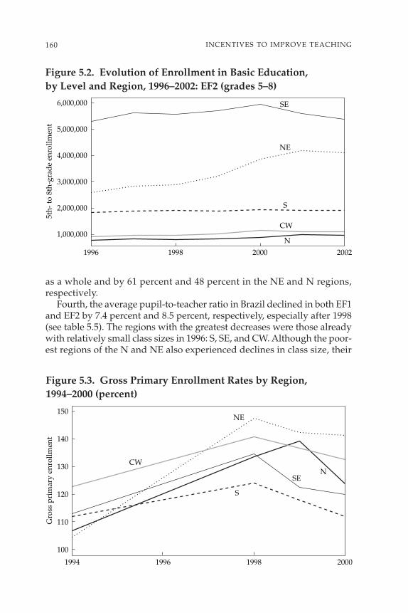
160 INCENTIVES TO IMPROVE TEACHING
1,000,000
2,000,000
3,000,000
4,000,000
5,000,000
6,000,000
5th-
to 8
th-g
rad
e en
rollm
ent
1996 1998 2000 2002
N
NE
S
SE
CW
Figure 5.2. Evolution of Enrollment in Basic Education, by Level and Region, 1996–2002: EF2 (grades 5–8)
100
110
120
130
140
150
Gro
ss p
rim
ary
enro
llmen
t
1994 1996 1998 2000
N
NE
S
SE
CW
Figure 5.3. Gross Primary Enrollment Rates by Region,1994–2000 (percent)
as a whole and by 61 percent and 48 percent in the NE and N regions,respectively.
Fourth, the average pupil-to-teacher ratio in Brazil declined in both EF1and EF2 by 7.4 percent and 8.5 percent, respectively, especially after 1998(see table 5.5). The regions with the greatest decreases were those alreadywith relatively small class sizes in 1996: S, SE, and CW. Although the poor-est regions of the N and NE also experienced declines in class size, their

average pupil-to-teacher ratios in basic education in 2002 were the high-est in the country and, in some cases, were as high as the 1996 values of themore industrial regions.
Fifth, as shown in figure 5.5, the poorest regions of the N and NE madegreat strides to catch up with the more industrial regions of the S, SE, andCW in terms of the percentage of teachers for grades 1–4 (EF1) who hadcompleted credentials of higher than primary education. By 2002, almostall teachers in Brazil had acquired the minimum required training.
161EDUCATIONAL FINANCE EQUALIZATION
75
80
85
90
95
100
Net
pri
mar
y en
rollm
ent
1994 1996 1998 2000
N
NE
S
SE
CW
Figure 5.4. Net Primary Enrollment Rates by Region, 1994–2000 (percent)
Table 5.4. Number of Teachers by Level, Region, and YearEF1 EF2
1997–2002 1997–2002 change change
Region 1997 2000 2002 (percent) 1997 2000 2002 (percent)
N 67,678 72,463 72,090 6.52 32,202 41,684 47,795 48.42
NE 250,184 262,443 245,511 −1.87 116,315 158,923 187,660 61.34
SE 225,779 226,882 234,357 3.80 226,576 262,693 264,404 16.70
S 105,146 102,018 101,124 −3.83 99,877 107,002 114,427 14.57
CW 44,950 48,334 47,699 6.12 41,287 52,241 53,343 29.20
Total 693,737 712,140 700,781 1.02 516,257 622,543 667,629 29.32

162 INCENTIVES TO IMPROVE TEACHING
Table 5.5. Mean Pupil-to-Teacher Ratio by Level, Region, and YearEF1 EF2
1996–2002 1996–2002 change change
Region 1996 2000 2002 (percent) 1996 2000 2002 (percent)
N 31.2 31.0 30.0 −3.8 26.1 28.0 24.4 −6.5
NE 30.0 29.5 28.5 −5.0 24.7 27.7 26.7 8.1
S 22.8 22.2 21.8 −4.4 17.8 16.9 16.0 −10.1
SE 31.3 29.6 28.2 −9.9 26.9 22.3 20.8 −22.7
CW 30.3 26.4 25.4 −16.2 23.1 22.5 21.8 −5.6
All regions 29.6 28.4 27.4 −7.4 24.6 23.8 22.5 −8.5
0
0.2
0.4
0.6
Perc
enta
ge o
f unt
rain
ed te
ache
rs
1996 1998 2000 2002
N
NE
S
SE
CW
Figure 5.5. Percentage of Qualified Teachers by Region, 1996–2002
Finally, the average years of age-by-grade distortion declined in EF1 andincreased in EF2 (see table 5.6). This shift could reflect a possible reformeffect in which more age-appropriate children began to enroll in the firstyear of the primary level, thus decreasing late entry into first grade. In addi-tion, more older children may have returned to the higher grades of basiceducation after abandoning school, thus increasing age-by-grade distortionin EF2. This shift may reflect changes in demographic patterns. The trend
Table 5.6. Age-by-Grade Distortion by Region, Level, and Year(mean and standard deviation)
EF1 EF2
1996–2002 1996–2002 change change
Region 1996 2000 2002 (percent) 1996 2000 2002 (percent)
N 2.46 2.14 1.86 −24.4 1.99 2.95 2.72 36.7(0.47) (0.70) (0.71) (0.23) (0.67) (0.84)
NE 2.86 2.87 2.36 −17.5 2.21 3.66 3.35 51.6(0.61) (0.95) (0.99) (0.27) (0.64) (0.66)
S 0.83 0.70 0.62 −25.3 1.12 1.4 1.24 10.7(0.21) (0.31) (0.32) (0.25) (0.33) (0.40)
SE 1.16 0.98 0.84 −27.6 1.42 1.74 1.48 4.2(0.28) (0.49) (0.48) (0.17) (0.61) (0.64)
CW 1.73 1.50 1.38 −20.2 1.79 2.71 2.35 31.3(0.40) (0.44) (0.48) (0.24) (0.49) (0.48)
Total 1.77 1.68 1.43 −19.2 1.68 2.51 2.25 33.9(0.92) (1.11) (1.00) (0.46) (1.09) (1.08)
Note: Standard deviations are in parentheses.
163EDUCATIONAL FINANCE EQUALIZATION
toward lower fertility rates means that new cohorts of children are smallerin number as time goes by and that the demographic pressure in lower pri-mary is easing up at the same time as the “bulge” is entering upper pri-mary and secondary levels. We will explore these dynamics further in thediscussions that follow.
Financial Data
Our primary resource for financial data in 1996–2002 was the BrazilianSecretariat of the National Treasury (Secretaria do Tesouro Nacional, orSTN). The STN Web site offers information on annual state and munici-pal revenue from a number of federal transfers. Those transfers includethe State Participation Fund (Fundo de Participação dos Estados, orFPE); the Municipal Participation Fund (Fundo de Participação dosMunicípios, or FPM); and various transfers that go to both states andmunicipalities, including the tax on financial operations (imposto sobreoperações financeiras, or IOF), the tax on industrialized products relativeto exports (imposto sobre produtos industrializados, or IPI-exp), the taxon rural territorial property (imposto sobre a propiedade territorial rural,

or ITR), and various components of the Complementary Law 87 (LC87/96).55
STN also gives information on FUNDEF revenue to each municipalityand state as well as on state and municipal spending. We used the Educa-tion and Culture spending to calculate per pupil expenditure. In only oneyear (2002) and for only the states was information available separately forEducation and Culture expenditure. In that year, state spending on culturewas on average 2.2 percent of Education and Culture spending (rangingfrom 0.06 percent to 7.25 percent).
Table 5.7 reports the FUNDEF state allocations from 1998 through 2002and the minimum spending floor mandated each year. The table showsthat FUNDEF may be more effective in addressing within-state inequal-ity in educational spending than inequality across states. Substantialinequalities in per pupil FUNDEF revenue exist along historical lines ofregional economic and social inequalities in the country. The NE states ofBrazil, specifically, tended to have smaller per pupil FUNDEF allocationsthan wealthier and more industrial states.
Table 5.8 shows the mean per pupil spending in constant values, byregion and year. The means provide evidence of the great inequality in perpupil spending across regions in Brazil while the large standard deviationsreveal within-region inequality. The table also indicates that educationalexpenditures in all regions increased in the 1996–2002 period, especially inthe SE, N, and NE. Given that the N and NE regions are the two poorestof the country, the substantial increase in real per pupil spending in thoseregions suggests that the reform is having much of the desired effect.However, because the reform establishes only a minimum spending perpupil, wealthy areas such as the SE region have been able to increasespending at a faster rate than less advantaged areas.
Table 5.9 reports mean net FUNDEF allocations in per pupil terms andmean per pupil expenditures by year (a) for the top and bottom 20 per-cent of municipalities in terms of FUNDEF net allocations in 1998 and (b) for the full sample. The figures suggest that FUNDEF losers were, forthe most part, mature systems with high per pupil expenditures. Thus, inlosing resources, they were unable to reduce educational expenditures.FUNDEF winners were able to substantially increase their per pupil expen-ditures in 1998–2002, which suggests that the reform led to a crowd-in of
164 INCENTIVES TO IMPROVE TEACHING
55. The only tax that contributes to FUNDEF but is not available from STN is the statetax on the circulation of goods and the tendering of interstate and intermunicipal trans-portation and communication services (imposto sobre operações relativas à circulação demercadorias e sobre serviços de transporte interestadual e intermunicipal e de comunicação,ainda que as operações se iniciem no exterior, or ICMS). The revenue generated from thisstate tax was available on the Web site of the Central Bank. The data are available by state andyear from 1996 to 2002. One-fourth of the revenue generated from the ICMS tax is distributedby each state to its municipalities. We used those data in our calculations of FUNDEF and ofrevenue earmarked for education.
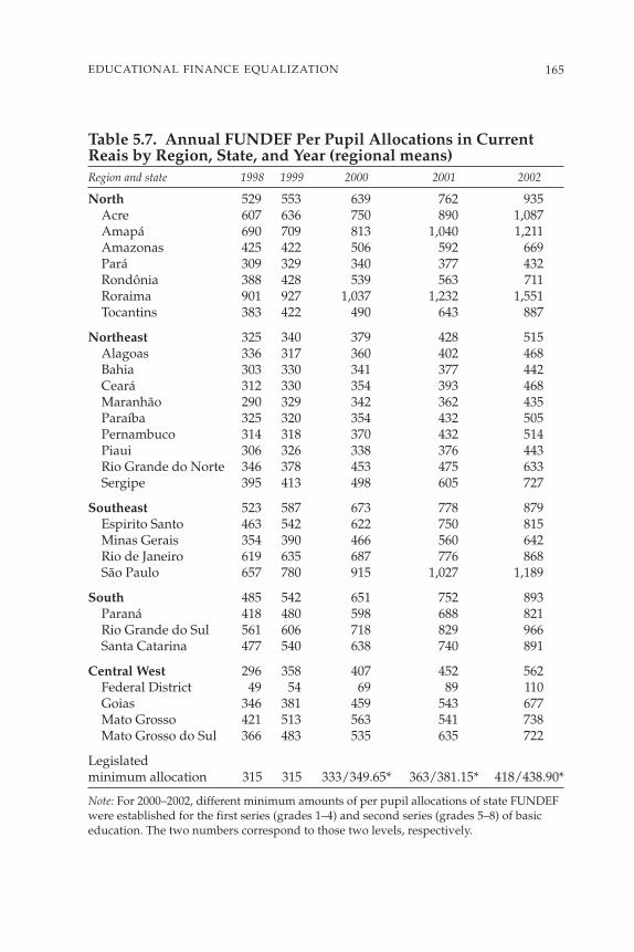
165EDUCATIONAL FINANCE EQUALIZATION
Table 5.7. Annual FUNDEF Per Pupil Allocations in CurrentReais by Region, State, and Year (regional means)Region and state 1998 1999 2000 2001 2002
North 529 553 639 762 935Acre 607 636 750 890 1,087Amapá 690 709 813 1,040 1,211Amazonas 425 422 506 592 669Pará 309 329 340 377 432Rondônia 388 428 539 563 711Roraima 901 927 1,037 1,232 1,551Tocantins 383 422 490 643 887
Northeast 325 340 379 428 515Alagoas 336 317 360 402 468Bahia 303 330 341 377 442Ceará 312 330 354 393 468Maranhão 290 329 342 362 435Paraíba 325 320 354 432 505Pernambuco 314 318 370 432 514Piaui 306 326 338 376 443Rio Grande do Norte 346 378 453 475 633Sergipe 395 413 498 605 727
Southeast 523 587 673 778 879Espirito Santo 463 542 622 750 815Minas Gerais 354 390 466 560 642Rio de Janeiro 619 635 687 776 868São Paulo 657 780 915 1,027 1,189
South 485 542 651 752 893Paraná 418 480 598 688 821Rio Grande do Sul 561 606 718 829 966Santa Catarina 477 540 638 740 891
Central West 296 358 407 452 562Federal District 49 54 69 89 110Goias 346 381 459 543 677Mato Grosso 421 513 563 541 738Mato Grosso do Sul 366 483 535 635 722
Legislated minimum allocation 315 315 333/349.65* 363/381.15* 418/438.90*
Note: For 2000–2002, different minimum amounts of per pupil allocations of state FUNDEFwere established for the first series (grades 1–4) and second series (grades 5–8) of basiceducation. The two numbers correspond to those two levels, respectively.

educational expenditures. We will further address this question in ourregression analyses.
Student Achievement Data
The Sistema Nacional de Avaliação da Educação Básica (National Systemfor Basic Education Evaluation, or SAEB) is a national educational assess-ment system administered approximately every 2 years beginning in 1995.It contains standardized exams in math and Portuguese, as well as ques-tionnaires to students, teachers, and school directors. In 2003, it wasadministered to 300,000 students and 17,000 teachers.
With respect to our study, one limitation of SAEB is that—although theassessment is conducted in all 26 states (and the Federal District) ofBrazil—the data cannot be disaggregated at the municipal level. Instead,the test results are representative only for state, municipal, and privateschools at the state level.
Tables 5.10 and 5.11 present means, standard deviations, and the Giniinequality coefficient56 of SAEB language and mathematics test scores by
166 INCENTIVES TO IMPROVE TEACHING
Table 5.8. Mean Per Pupil Spending, by Region and Year (in constant 1995 reais)
1996–2002Region 1996 2000 2002 change (percent)
N 614 777 880 43.4(275) (278) (370)
NE 466 562 673 44.4(218) (256) (411)
S 978 1,226 1,277 30.6(391) (382) (357)
SE 890 1,354 1,513 70.0(498) (720) (501)
CW 844 1,005 1,055 25.0(450) (518) (466)
All regions 751 1,010 1,120 49.1(450) (626) (572)
Note: To convert current per pupil spending into constant values, we used the gross domesticproduct deflator in constant national currency from the IMF’s International Financial Statistics(2004). The real-to-U.S. dollar exchange rate devaluated substantially during this period. In 1996, the exchange rate was approximately 1:1; by 2002, it was 2.92:1 (IMF 2004).
56. The Gini inequality coefficient (or concentration ratio) expresses the overall inequalitypresent in a distribution. It has a theoretical range from 0 (perfect equality) to 1 (perfectinequality).

167EDUCATIONAL FINANCE EQUALIZATION
Table 5.9. Mean Net FUNDEF Per Pupil Allocation and MeanPer Pupil Expenditures, 1998–2002 (in reais)
Top 20 percent of Bottom 20 percent ofmunicipalities by net municipalities by net
Year Full sample FUNDEF per pupil in 1998 FUNDEF per pupil in 1998
Mean net FUNDEF per pupil:1998 −76.73901 242.0814 −704.92581999 −80.96458 254.6308 −666.40012000 −33.41097 280.7323 −640.70482001 −12.48755 313.1553 −667.68352002 28.05855 388.3044 −635.4375Average 1998–2002 −34.51019 288.6141 −665.3754
Mean per pupil expenditure:1996 1,295.196 525.0750 2,621.6891998 1,528.070 679.7418 3,118.2981999 1,646.889 772.7175 3,028.9612000 1,737.586 894.8524 3,274.6382001 1,834.941 1,001.1100 3,504.2722002 1,791.767 1,057.6790 3,153.661Average 1996–2002 1,718.390 869.5564 3,209.397
Table 5.10. Means, Standard Deviations, and Gini Coefficientsfor SAEB Language Scores in 1995, 2001
1995 2001
Region Mean Gini Mean Gini
N 174.90 0.14 164.57 0.16(42.54) (46.28)
NE 181.26 0.14 161.85 0.17(45.35) (47.92)
SE 197.71 0.13 187.92 0.16(46.37) (52.62)
S 197.11 0.13 188.98 0.15(45.81) (48.39)
CW 193.92 0.13 175.19 0.17(43.20) (51.29)
National 187.17 0.14 171.71 0.17(45.72) (50.27)
Note: Standard deviations are in parentheses.

168 INCENTIVES TO IMPROVE TEACHING
Table 5.11. Means, Standard Deviations, and Gini Coefficientsfor SAEB Mathematics Scores in 1995, 2001
1995 2001
Region Mean Gini Mean Gini
N 176.24 0.10 172.63 0.14(31.96) (42.72)
NE 182.28 0.12 172.90 0.15(38.20) (45.50)
SE 199.92 0.12 200.28 0.15(42.14) (51.71)
S 193.91 0.11 201.53 0.13(38.94) (46.09)
CW 193.54 0.11 187.56 0.15(39.06) (49.65)
National 187.85 0.12 182.85 0.15(39.18) (48.37)
Note: Standard deviations are in parentheses.
region for 1995 (pre-FUNDEF) and 2001 (post-FUNDEF). As expected,students in the N and NE regions have lower average test scores than dostudents in the wealthier regions of the country. Overall, the Gini coeffi-cients are small in relative terms, indicating that the variation in studenttest scores among and between regions is not substantial. Surprisingly,given the equalization objectives of the reform, there appears to have beena slight increase in test score inequality in all regions during 1995–2001.
Empirical Strategy
We used various strategies to address our set of research questions. Wegrouped our empirical strategies by the nature of our three mainresearch objectives: (a) assessing the effect of FUNDEF-induced spend-ing on state-level enrollment, (b) evaluating system-level mean effects ofFUNDEF-induced spending on educational inputs and outcomes, and(c) evaluating the distributional effects of FUNDEF-induced resourceson student achievement.
Although the FUNDEF reform was a major force underlying shifts inthe allocation of educational resources beginning in 1998, as discussedearlier, it took place at a time of much education reform in Brazil. Thus, thediscussion of pre- and post-reform effects does not solely explain the effectof the reform. For example, as FUNDEF overhauled the educationalfinance in Brazil, the government mandated that teachers must have at

least a secondary education degree, thus eliminating the existence ofleigos teachers—teachers who had completed only primary school. Thecombination of increased resources for some municipalities and of thismandate is associated with a sharp increase in some states and munici-palities in their share of teachers with higher than primary education cre-dentials in the late 1990s, as shown earlier. The policy evaluation problemis complicated by the fact that the two mandates were implementednationally and at the same time. Any uniform effect of the teacher educa-tion mandate will be captured with the year fixed effects. However, if theeffect of that mandate varies with FUNDEF-induced spending (for exam-ple, if systems with higher spending can more easily eliminate untrainedteachers), then our ordinary least squares (OLS), instrumental variable(IV), and reduced-form regression frameworks will attribute that varyingeffect—along with the direct effects of spending—to FUNDEF.
Assessing the Effect of FUNDEF-Induced Spending on State-Level Enrollment
One of the explicit goals of FUNDEF is to increase enrollment throughoutBrazil by guaranteeing the availability of the minimum level of resourcesneeded to meet the legal mandate of mandatory schooling in grades 1–8 inall municipal and state systems. Although narrowing the enrollment rategap was not explicitly a goal of FUNDEF, it is a fundamental concern notonly for education policymakers throughout the world but also for theinternational donor community in the context of the Millennium Devel-opment Goals.57
As shown in table 5.1, enrollment rates varied considerably withinBrazil before the FUNDEF reform. The net enrollment rate, which is thepercentage of age-appropriate children enrolled in fundamental educa-tion, ranged from 77.3 percent in the NE region to 94.4 percent in the SEregion in 1994. This difference reflects both wide regional disparities andan overall enrollment rate that is far from universal (the countrywide fun-damental education enrollment rate is 87.5 percent).
Figures 5.1 and 5.2 show that the timing of the FUNDEF reform coin-cided with both increased average enrollment and decreased inequality inenrollment rates across regions. Enrollment rates are influenced by a num-ber of factors beyond the school finance environment, however, so we can-not interpret those trends as indicative of a causal relationship. Figure 5.1shows that enrollment increased in the early 1990s and in the mid- and late-1990s, which cannot be explained by FUNDEF (Duryea, Lam, and Levinson2003). Duryea, Lam, and Levinson point out the intuitive and empirically
169EDUCATIONAL FINANCE EQUALIZATION
57. In September 2000, members of the United Nations unanimously adopted the Millennium Declaration, which establishes eight Millennium Development Goals to beachieved by 2015, including universal primary education.

observed tradeoff between child labor and schooling, and they describedeclining child labor in the 1990s (including declines before the introduc-tion of FUNDEF). Lam and Marteleto (2002) analyze the decision to enrollstudents in school at the individual level, and they find that increasinglevels of parental education, decreasing family size, and decreasing cohortsize all contributed to increasing enrollment rates in the 1990s.
To avoid conflating the effects of the reform with these other contribu-tors to enrollment growth, we focused on how the amount of spendingattributable to the FUNDEF reform affects enrollment. Because the reformalso has been associated with shifts from state schools to municipalschools, we conducted our analysis at the state rather than system level.(Note that shifts from municipal schools to state schools within a state willshow up as no change in state-level enrollment, so state-level totals willmore accurately reflect changes in the number of children enrolled in anypublic school.) Our approach is quite similar to the empirical strategiesalready described, with the main difference being that the data are aggre-gated up to the state level. We estimated the following specifications:
We calculated results separately for enrollment in levels EF1 and EF2(grades 1–4 and grades 5–8, respectively). Ed Exps,y is aggregate spend-ing on fundamental education (total, not per pupil spending) in state s inyear y. The parameters αs and βy control for state and year fixed effects.In the specification from equation 5.2, we allow the effect of spending onenrollment to differ according to whether or not a state was bound by thefederal revenue floor instituted by FUNDEF. Those states (7 of the 27 total)were the only ones to receive positive net transfers from the federal gov-ernment as a result of the program. We first estimated equation 5.1 usingOLS. Then, to isolate spending changes that are within a state and are attrib-utable to the reform, we used the same instrumental variable approach asdescribed earlier, in which mandated spending under the current policyregime serves as an instrumental variable for actual spending.
Evaluating System-Level Mean Effects of FUNDEF-Induced Spending on Educational Inputs and Outcomes
We investigated the effect of the FUNDEF reform on educational inputsand outcomes first in an OLS regression, then with IV and reduced formapproaches that use the funding formula to isolate changes in inputs that
( . ) *
* *, ,
, ,
5 2 Enrollment y Ed Exp
Ed Exp BOUND
s y s y s y
s y s s y
= + +
+ +
α β
δ ε
( . ) *, , ,5 1 Enrollment y Ed Exps y s y s y s y= + + +α β ε
170 INCENTIVES TO IMPROVE TEACHING
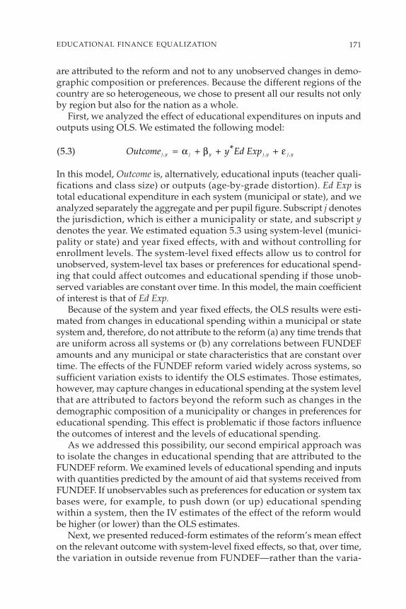
are attributed to the reform and not to any unobserved changes in demo-graphic composition or preferences. Because the different regions of thecountry are so heterogeneous, we chose to present all our results not onlyby region but also for the nation as a whole.
First, we analyzed the effect of educational expenditures on inputs andoutputs using OLS. We estimated the following model:
In this model, Outcome is, alternatively, educational inputs (teacher quali-fications and class size) or outputs (age-by-grade distortion). Ed Exp istotal educational expenditure in each system (municipal or state), and weanalyzed separately the aggregate and per pupil figure. Subscript j denotesthe jurisdiction, which is either a municipality or state, and subscript ydenotes the year. We estimated equation 5.3 using system-level (munici-pality or state) and year fixed effects, with and without controlling forenrollment levels. The system-level fixed effects allow us to control forunobserved, system-level tax bases or preferences for educational spend-ing that could affect outcomes and educational spending if those unob-served variables are constant over time. In this model, the main coefficientof interest is that of Ed Exp.
Because of the system and year fixed effects, the OLS results were esti-mated from changes in educational spending within a municipal or statesystem and, therefore, do not attribute to the reform (a) any time trends thatare uniform across all systems or (b) any correlations between FUNDEFamounts and any municipal or state characteristics that are constant overtime. The effects of the FUNDEF reform varied widely across systems, sosufficient variation exists to identify the OLS estimates. Those estimates,however, may capture changes in educational spending at the system levelthat are attributed to factors beyond the reform such as changes in thedemographic composition of a municipality or changes in preferences foreducational spending. This effect is problematic if those factors influencethe outcomes of interest and the levels of educational spending.
As we addressed this possibility, our second empirical approach wasto isolate the changes in educational spending that are attributed to theFUNDEF reform. We examined levels of educational spending and inputswith quantities predicted by the amount of aid that systems received fromFUNDEF. If unobservables such as preferences for education or system taxbases were, for example, to push down (or up) educational spendingwithin a system, then the IV estimates of the effect of the reform wouldbe higher (or lower) than the OLS estimates.
Next, we presented reduced-form estimates of the reform’s mean effecton the relevant outcome with system-level fixed effects, so that, over time,the variation in outside revenue from FUNDEF—rather than the varia-
( . ) *, , ,5 3 Outcome y Ed Expj y j y j y j y= + + +α β ε
171EDUCATIONAL FINANCE EQUALIZATION

tion in spending or input levels—within each municipal or state systemidentifies changes in other variables. The simplest way to think of the dis-tinction between the IV and the reduced-form approaches is that the IVapproach uses policy-induced, exogenous variation to identify the effect ofspending on student outcomes whereas the reduced-form approach iden-tifies the effect of the revenue from the policy itself on outcomes. We esti-mated the following model:
In this model, Outcome and all subscripts are defined as before. Mandatedis the total revenue mandated to be spent on basic education, which variesdepending on whether the year is before or after realization of FUNDEF.Before 1998, Mandated equaled 25 percent of all contributing taxes andtransfers. In 1998 and after, it equaled 10 percent of the taxes and trans-fers that contribute to the FUNDEF account, 25 percent of the noncon-tributing taxes and transfers, and payments from FUNDEF. Also note thatactual payments to municipal and state systems from FUNDEF vary withenrollment or, more specifically, with a school system’s share of total currentenrollment in that state. Estimating the effect of the reform on enrollment,however, is of independent interest to our study. We, therefore, estimatedthe effect of the Mandated variable on inputs and outputs by holding theenrollment share of each school system (within its state) constant over timeat its level before the realization of the reform. As before, we estimatedequation 5.4 using system-level (municipality or state) fixed effects, withand without controlling for enrollment levels. We also estimated per pupilvariations of that equation in which educational spending and revenuemandated for education are both in per pupil terms. In this model, the maincoefficient of interest is that of Mandated.
In addition to exploring the effects of spending on inputs to and outputsfrom the education production function, we also directly examined theproduction function itself. We did this by analyzing the effect of inputs(again, class size and teacher training) on student outcomes. The setupwas the same as in the previous analyses: (a) variables are year and systemfixed effects, (b) OLS looks at direct effects of inputs, and (c) the IVapproach uses mandated spending as an instrument for actual inputs.
Evaluating the Distributional Effects of FUNDEF-Induced Resources on Student Achievement
Because our student achievement data are representative only at the stateand not at the municipal level, we explored the effect of the distributionalchanges in resources on student achievement, asking whether more equal-ized spending and inputs help to close the gap in student outcomes. Thus,
( . ) *, , ,5 4 Outcome y Mandatedj y j y j y j y= + + +α β ε
172 INCENTIVES TO IMPROVE TEACHING
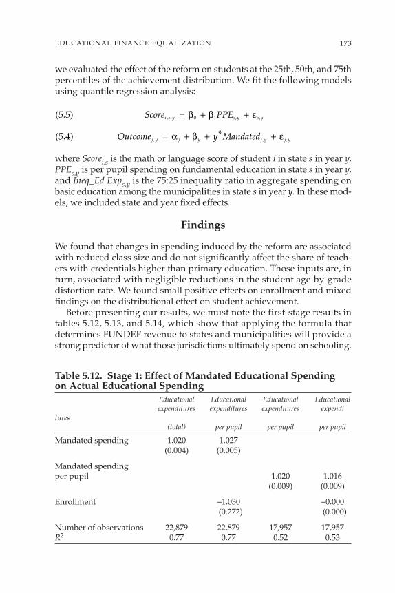
we evaluated the effect of the reform on students at the 25th, 50th, and 75thpercentiles of the achievement distribution. We fit the following modelsusing quantile regression analysis:
where Scorei,s is the math or language score of student i in state s in year y,PPEs,y is per pupil spending on fundamental education in state s in year y,and Ineq_Ed Exps,y is the 75:25 inequality ratio in aggregate spending onbasic education among the municipalities in state s in year y. In these mod-els, we included state and year fixed effects.
Findings
We found that changes in spending induced by the reform are associatedwith reduced class size and do not significantly affect the share of teach-ers with credentials higher than primary education. Those inputs are, inturn, associated with negligible reductions in the student age-by-gradedistortion rate. We found small positive effects on enrollment and mixedfindings on the distributional effect on student achievement.
Before presenting our results, we must note the first-stage results intables 5.12, 5.13, and 5.14, which show that applying the formula thatdetermines FUNDEF revenue to states and municipalities will provide astrong predictor of what those jurisdictions ultimately spend on schooling.
( . ) *, , ,5 4 Outcome y Mandatedj y j y j y j y= + + +α β ε
( . ) , , , ,5 5 0 1Score PPEi s y s y s y= + +β β ε
173EDUCATIONAL FINANCE EQUALIZATION
Table 5.12. Stage 1: Effect of Mandated Educational Spending on Actual Educational Spending
Educational Educational Educational Educationalexpenditures expenditures expenditures expendi
tures(total) per pupil per pupil per pupil
Mandated spending 1.020 1.027(0.004) (0.005)
Mandated spending per pupil 1.020 1.016
(0.009) (0.009)
Enrollment −1.030 −0.000(0.272) (0.000)
Number of observations 22,879 22,879 17,957 17,957R2 0.77 0.77 0.52 0.53

Tables 5.12, 5.13, and 5.14 show results from estimating equation 5.4 withactual educational spending, either total spending or per pupil spending,as the dependent variable as opposed to other inputs or outcomes.
For ease of interpretation, we prefer the per pupil specification ofinputs on outcomes, so our preferred specifications in table 5.12 are incolumns 3 and 4. The inclusion of enrollment as a control does not affectthe strength with which formula-driven, mandated spending predictsactual spending (compare columns 3 and 4). The coefficient on mandatedspending (in column 3) is 1.02, which is highly statistically significant witha standard error of 0.009. The R2 for the specification is 0.52. Table 5.13shows that this predictive power holds across all regions of the country,and table 5.14 shows that it is also robust across all post-reform years forwhich we have data.
The fact that mandated spending per pupil predicts actual spendingper pupil with such strong t statistics is important for the validity of theinstrumental variables and reduced-form estimations that follow. Thatmandated spending predicts actual spending with coefficients so close to
174 INCENTIVES TO IMPROVE TEACHING
Table 5.13. Stage 1: Effect of Mandated Educational Spending on Actual Per Pupil Educational Spending, by Geographic Region
N NE S SE CW
Mandated spending 1.134 1.065 1.046 1.138 0.799 per pupil (0.057) (0.022) (0.019) (0.014) (0.038)
Enrollment −0.000 −0.000 −0.001 −0.000 −0.001(students) (0.000) (0.000) (0.000) (0.000) (0.000)
Number of observations 1,253 7,022 6,000 6,690 1,914
R2 0.63 0.59 0.51 0.70 0.43
Note: Standard errors are in parentheses.
Table 5.14. Stage 1: With Year-Specific Predictors1998 1999 2000 2001 2002
Mandated spending per pupil 0.984 1.005 0.962 0.979 1.012(0.016) (0.015) (0.015) (0.016) (0.016)
Enrollment −0.001 −0.000 −0.000 −0.000 −0.000(0.000) (0.000) (0.000) (0.000) (0.000)
Number of observations 6,091 6,121 6,649 6,730 6,294
R2 0.62 0.64 0.60 0.63 0.65
Note: Standard errors are in parentheses.
one is informative independently. States and municipalities can devotesome additional revenue beyond that mandated for educational spending.A coefficient less than 1 (for example, 0.8) would suggest that jurisdictionsreduced their voluntary educational revenue efforts by 20 percent of anincrease in mandated spending per pupil, whereas a coefficient greater than1 (for example, 1.5) would suggest that jurisdictions increased their volun-tary educational revenue efforts by 50 percent of an increase in mandatedspending per pupil. Our results suggest quite small and statistically insignif-icant crowd-out, with a point estimate of under 2 percent in 1998, the firstyear of implementation. For each year that follows, the coefficients are sta-tistically insignificantly different from 1, suggesting that the reform led tothe planned increase in educational expenditures. That those coefficients areso close to 1 also explains why the OLS estimates are so similar to the IV esti-mates: FUNDEF allocations by the state, rather than unobserved changesin preferences or local responses to the reform, were largely responsible forchanges in spending at the local level over this period.
Effects of FUNDEF-Induced Spending on State-Level Enrollment
Table 5.15 presents OLS and IV results for the state-level analysis of theeffect that FUNDEF-induced spending has on enrollment levels (estimatedfrom equation 5.1). FUNDEF appears to be driving the bulk of the varia-tion over time within jurisdictions (here, within states), so the OLS andIV estimates are quite similar. We have aggregated the data used in ourestimates from all the municipalities and the state system for each year.The number of municipal systems reporting varies by year. This variationmay reflect not only changes in school system organization such as con-solidation but also missing data. Missing data are not a problem in themunicipal-level analyses, which contain municipal fixed effects. In the
175EDUCATIONAL FINANCE EQUALIZATION
Table 5.15. State-Level Effects of Spending on Enrollment, by LevelEF1 (grades 1–4) EF2 (grades 5–8)
OLS IV OLS IV
Educational spending −0.004 −0.005 −0.002 −0.001(0.001) (0.001) (0.001) (0.001)
Educational spending × bound 0.007 0.004 0.022 0.025 by FUNDEF floor (0.004) (0.004) (0.002) (0.003)
State-year observations 162 162 162 162
State observations 27 27 27 27
Note: Standard errors are in parentheses.

aggregated case, the state observation will not be missing, even if there aremissing components. More municipalities reported in 1996 than in lateryears. If this decrease is driven by systematically lower reporting ratesafter the reform, then the results will be biased toward finding declines inenrollment. Another impetus for the aggregation is that an effect of thereform appears to have been that municipal systems now focus on pro-viding basic education (grades 1–8), while state education systems areincreasingly focusing on post-basic education. By aggregating to the statelevel, therefore, we are evaluating the effect of the reform on actualchanges in enrollment and not on transfers between municipal systemsor flows of students from state systems to municipal, or vice versa.
Table 5.15 describes the type of result for EF1 that could be attributedto decreases in reporting rates by municipal systems: The OLS and IVestimates both report statistically significant but economically negligibleeffects of spending on enrollment. Because our financial data are in hun-dreds of reais, the −0.005 coefficient on spending for EF1 enrollment inthe IV specification means that a R$100,000 increase in spending,statewide, would reduce EF1 enrollment by five students. For EF1 enroll-ment, there is no differential effect for whether or not a state is bound bythe federal floor of educational revenue per pupil (the coefficient on edu-cational spending × bound by floor is insignificant).
The results for EF2 enrollment, however, present a different picture. Forstates that are not bound by the FUNDEF floor, the effect of FUNDEF-induced spending on enrollment is statistically insignificant for the IVspecification. For states that are bound by the floor, however, enrollmentincreases with spending. To interpret the 0.025 coefficient, we should con-sider the mean total spending increase of about R$190 million from 1996 to1998 among states bound by the floor. An increase of this kind predicts anincrease in EF2 enrollment to slightly fewer than 5,000 students. Mean EF2enrollment for those states was 353,935 in 1996 and 386,672 in 1998. Thepredicted increase is, therefore, less than 2 percent of base enrollment andaccounts for 15 percent of the total observed increase in EF2 enrollmentsfrom 1996 to 1998. Although this effect is not huge, the data do indicatethat spending was more positively associated with enrollment gains ingrades 5–8 in the states that benefited the most from the reform. (Thosestates also had the lowest initial enrollment rates, but analyzing the inter-action between spending and pre-FUNDEF enrollment rates, not shown,yields statistically insignificant responses.)
System-Level Mean Effects of FUNDEF-Induced Spending on Educational Inputs and Outcomes
In the paragraphs that follow, we evaluate the effect of FUNDEF on edu-cational inputs and outcomes. In particular, we focus on how systems
176 INCENTIVES TO IMPROVE TEACHING

responded to the changed levels of resources available for educationresulting from FUNDEF in decisions about class sizes and teacher qualifi-cations. In addition, we explore the effect of the reform on student out-comes, specifically age-by-grade distortion rates and the distribution ofstudent achievement.
Effects of FUNDEF-Induced Spending on InputsHow did school systems spend the money they received from FUNDEF?Conversely, for those systems losing money, how did they cut back? Wefocused on two key variables: the teacher-to-pupil ratio and the share ofteachers with credentials of only primary education.58 We analyzed bothvariables at the EF1 and EF2 levels separately. We presented estimatesfrom the OLS, IV, and reduced-form specifications of spending on classsize in table 5.16 and on the share of teachers with credentials higher thanprimary education in table 5.17.
Table 5.16 shows that increasing mandated spending has a statisticallysignificant and negative effect on class size at both the EF1 and EF2 levels.If we interpret the coefficients, the IV point estimate of −0.184 for EF1class size implies that an increase of R$1,000 in mandated spending perpupil is associated with a reduction in class size of 1.84 students. (Recallthat mean spending per pupil, in all levels combined, increased fromabout R$750 to a little more than R$1,100 from 1996 to 2000.) For EF2, anincrease of R$1,000 in mandated spending per pupil would lead to a pre-dicted decrease in class size by 2.1 students.
The findings on teacher training generally are not statistically significant,and the point estimates are not economically significant. From the com-parison of means, we know that the share of teachers with more educationbackground was rising over this period, especially in EF1 and in the N and
177EDUCATIONAL FINANCE EQUALIZATION
Table 5.16. Effects of Educational Spending Per Pupil on Class Size, by Level
EF1 (grades 1–4) EF2 (grades 5–8)
OLS IV Reduced form OLS IV Reduced form
Spending −0.127 −0.184 −0.166 −0.208per pupil (0.004) (0.007) (0.031) (0.044)
Mandatedexpenditures −0.185 −0.218per pupil (0.007) (0.047)
Number of observations 23,460 17,954 18,002 16,445 12,873 12,903
R2 0.14 0.14 0.01 0.02
Note: Standard errors are in parentheses.

NE regions where the proportion of untrained teachers was highest. Thistrend is likely to be a direct result of the new requirement that teachers havesecondary degrees. The IV estimates for EF1 in table 5.17 show us that anadditional R$1,000 of spending per pupil increased the share of EF1 teacherswith credentials higher than primary education by 1.8 percentage points.The increase in the share of teachers with credentials higher than primaryeducation far exceeded this estimate: Teachers without secondary degreeswere nearly completely eliminated over this period in all areas of Brazil,so the mandate was likely influential beyond the scope of the FUNDEFrevenue received by a jurisdiction.
Effects of FUNDEF-Induced Spending and Inputs on Student OutcomesWe have seen that the revenue redistributed by the FUNDEF system cor-responds with changes in educational inputs and, in particular, to changesin class size. At the same time, teacher qualification rates changed, but thiswas independent of the FUNDEF redistribution. In this section of the chap-ter, we initially show how, first, spending and, then, class size and teacherqualification rates correlate with student outcomes. We used the averagenumber of years of age above the norm for a specific grade (known as age-by-grade distortion) as our outcome variable. Age-by-grade distortion usu-ally reflects not only late school entry but also repetition and periodic schooldropout and reentry. All three (late entry, dropout, reentry) have beenidentified as major obstacles in education in Brazil, as well as in the South
178 INCENTIVES TO IMPROVE TEACHING
Table 5.17. Effects of Educational Spending Per Pupil on Share of Teachers with Credentials Higher Than Primary Education, by Level
EF1 (grades 1–4) EF2 (grades 5–8)
OLS IV Reduced form OLS IV Reduced form
Spending 0.0001 0.0018 −0.0002 −0.0000 per pupil (0.0002) (0.0003) (0.0001) (0.0003)
Mandated expenditures 0.0018 −0.0000 per pupil (0.0003) (0.0003)
Number of observations 23,516 17,954 18,002 16,482 12,873 12,903
R2 0.32 0.34 0.02 0.02
Note: Standard errors are in parentheses.
58. We were unable to analyze how FUNDEF allocation is associated with teacher salariesbecause we could not find any municipal-level data on teacher salaries.
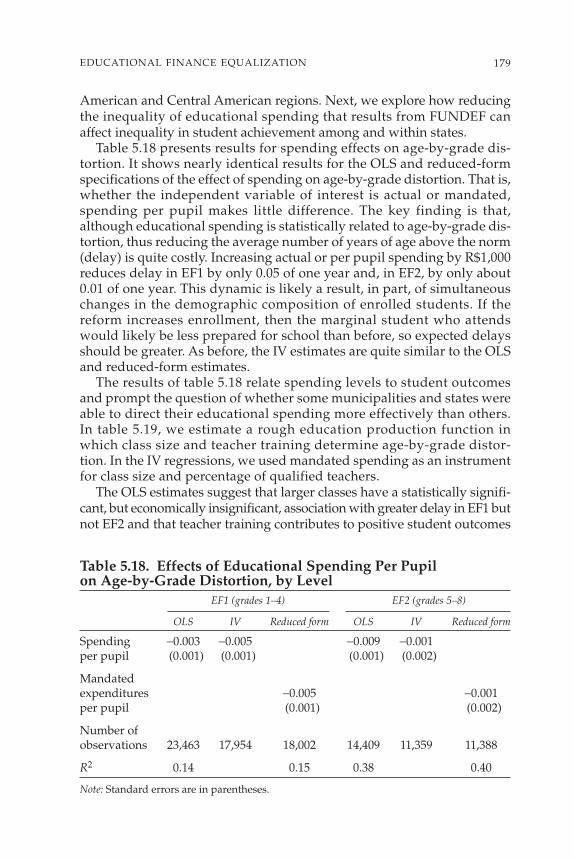
American and Central American regions. Next, we explore how reducingthe inequality of educational spending that results from FUNDEF canaffect inequality in student achievement among and within states.
Table 5.18 presents results for spending effects on age-by-grade dis-tortion. It shows nearly identical results for the OLS and reduced-formspecifications of the effect of spending on age-by-grade distortion. That is,whether the independent variable of interest is actual or mandated,spending per pupil makes little difference. The key finding is that,although educational spending is statistically related to age-by-grade dis-tortion, thus reducing the average number of years of age above the norm(delay) is quite costly. Increasing actual or per pupil spending by R$1,000reduces delay in EF1 by only 0.05 of one year and, in EF2, by only about0.01 of one year. This dynamic is likely a result, in part, of simultaneouschanges in the demographic composition of enrolled students. If thereform increases enrollment, then the marginal student who attendswould likely be less prepared for school than before, so expected delaysshould be greater. As before, the IV estimates are quite similar to the OLSand reduced-form estimates.
The results of table 5.18 relate spending levels to student outcomesand prompt the question of whether some municipalities and states wereable to direct their educational spending more effectively than others.In table 5.19, we estimate a rough education production function inwhich class size and teacher training determine age-by-grade distor-tion. In the IV regressions, we used mandated spending as an instrumentfor class size and percentage of qualified teachers.
The OLS estimates suggest that larger classes have a statistically signifi-cant, but economically insignificant, association with greater delay in EF1 butnot EF2 and that teacher training contributes to positive student outcomes
179EDUCATIONAL FINANCE EQUALIZATION
Table 5.18. Effects of Educational Spending Per Pupil on Age-by-Grade Distortion, by Level
EF1 (grades 1–4) EF2 (grades 5–8)
OLS IV Reduced form OLS IV Reduced form
Spending −0.003 −0.005 −0.009 −0.001 per pupil (0.001) (0.001) (0.001) (0.002)
Mandated expenditures −0.005 −0.001 per pupil (0.001) (0.002)
Number of observations 23,463 17,954 18,002 14,409 11,359 11,388
R2 0.14 0.15 0.38 0.40
Note: Standard errors are in parentheses.
in EF1 but not in EF2. A 10 percent increase in the share of teachers with cre-dentials higher than primary education corresponds to a statistically signifi-cant 0.05-year decline in average delay in EF1 and to a 0.005-year decline inEF2. The weaker result for EF2 reflects the small variation in the share ofEF2 teachers with credentials higher than primary education both before andafter the teacher education mandate. An increase of one student per teacheris associated with a 0.002-year increased delay in EF1, but there is no effect forEF2. The IV estimates are a bit stronger than the OLS estimates for EF2 andare quite similar for EF1. Interpreting the welfare effects of the estimateswould require valuing the negative effects of age-by-grade distortion andthen comparing them with local costs of class-size reduction.
Distributional Effects of FUNDEF-Induced Resources on Student Achievement
Because the SAEB standardized test scores are not representative at themunicipal level but they are at the state level, our evaluation of the effectof FUNDEF on student achievement necessarily focused on FUNDEF’seffect on the distribution of achievement among and within states. Ideally,we would have wished to analyze how the FUNDEF-induced, student-specific change in resources affected achievement. We analyzed the effectof the reform on the distribution of student achievement in math and lan-guage among states. We used quantile regression analysis to assess thedifferential effect of the reform at various levels of the achievement distri-bution. We conducted the same analyses for math and language, and theresults do not differ substantively. For ease of presentation herein, weinclude only the math achievement results.
Table 5.20 presents the effect of changes in mean actual per pupil spend-ing across states on the distribution of achievement among states. Ouranalyses included the effect of mean actual per pupil spending on the 25th,
180 INCENTIVES TO IMPROVE TEACHING
Table 5.19. Effects of Education Inputs on Age-by-Grade Distortion, by Level
EF1 (grades 1–4) EF2 (grades 5–8)
OLS IV OLS IV
Class size 0.002 0.023 0.000 0.005(0.001) (0.005) (0.000) (0.013)
Share of teachers with −0.488 −0.551 −0.049 −0.107 at least primary education (0.025) (0.031) (0.064) (0.079)
Observations 23,516 18,002 14,388 11,343
R2 0.16 0.38
Note: Standard errors are in parentheses.

50th, and 75th percentiles of the mathematics achievement distribution.The results in the table show that the effect of state-level, actual average,per pupil spending on student achievement does not differ by percentilesof the achievement distribution and that the effect is economicallyinsignificant. To interpret the coefficients, we must recall that the meanmathematics score for Brazil fell from 188 (standard deviation 39) in 1995to 183 (standard deviation 48) in 2002 and that mean spending per pupil inBrazil rose R$369, from R$751 in 1996 to R$1,120 in 2002. Applying thecoefficient at the median—the q(0.50) column—suggests that the meanR$369 increase in per pupil spending is associated with a 0.00369-point(or less than one-thousandth of a standard deviation) decline in mathachievement for the typical student. Though precisely estimated, thiseffect clearly is not behaviorally or economically significant.
Table 5.21 presents the results from an analysis of the effect that changesin actual spending inequality among states had on the distribution ofachievement. We use the ratio of the 75th to the 25th percentiles in meanactual per pupil expenditures as our measure of spending inequality. Thisratio was equal to 1.51 for all of Brazil in 1996 and equal to 2.35 in 2002(weighting school systems by their current enrollments).
The results in table 5.21 suggest that inequality in actual per pupilspending is associated with lower scores for students in the bottom per-
181EDUCATIONAL FINANCE EQUALIZATION
Table 5.20. Estimated Effect of Changes in State-Level Mean Per Pupil Spending on Mathematics Student Achievement by Percentile
q(0.25) q(0.50) q(0.75)
Actual mean per pupil spending −0.001 −0.001 −0.001(4.66e−11) (4.90e−17) (2.68e−11)
Pseudo R2 0.787 0.784 0.797
Number of observations 78 78 78
Notes: Standard errors are in parentheses. All models include year and state dummies.
Table 5.21. Estimated Effect of Changes in State-Level Inequality in Per Pupil Spending on Mathematics Student Achievement by Percentile
q(0.25) q(0.50) q(0.75)
Actual per pupil expenditure −1.213 0.843 1.135 inequality 75/25 (6.31e−09) (1.25e−14) (5.58e−15)
Pseudo R2 0.786 0.784 0.8
Number of observations 78 78 78
Notes: Standard errors in parentheses. All models include year and state dummies.
centiles of the achievement distribution and is associated with positiveeffects for students at the top. For example, the second panel of the tableshows that an increase of 1 in the state-level ratio of per pupil expendituresof the 75th to the 25th percentile is associated with a reduction of about1.2 points in student achievement of the students in the 25th percentile.In contrast, the same increase in this state-level inequality ratio is associ-ated with an increase of about 1.1 points in mean student achievement ofstudents in the 75th percentile. The direction of those effects is not sur-prising given that schools with higher socioeconomic status students tendto spend more and to have higher achievement levels. The unexpectedresult is, rather, that the magnitude of the relationship is so small.
Conclusions and Policy Implications
We find that the revenue flows from FUNDEF translated fully into educa-tional spending, suggesting that municipal and state governments used thenew funds as supplemental, thus not as substitutes, for their own revenue.From a policy perspective, this finding alone is important. Unlike many edu-cational finance reforms, FUNDEF succeeded in its goal of ensuring that theresources allocated to education by the reform were indeed used as intended.
We find that some part of the new influxes of revenue through the FUN-DEF system were used to reduce class size and that the federal legislationmandating that teachers have at least a secondary education degree wassuccessful. The improvements in both teacher education and class size arenegatively correlated with age-by-grade distortion, but we note that themagnitude of those correlations is quite small, particularly given their costs.
Although assessing the effect and cost-effectiveness of the class sizereduction on student achievement is beyond the scope of this paper, it is notclear that reductions in average class sizes would result in improvements instudent achievement in Brazil. First, compared with other middle-incomecountries, Brazil already has relatively small average class sizes. Second,the literature on the effect of class size on student achievement in theUnited States has shown, at best, inconclusive evidence that class sizereductions are associated with improvements in student learning.59 More-over, given the current average class size in Brazil, pursuing further reduc-tions in class size is probably not warranted from a fiscal standpoint.
182 INCENTIVES TO IMPROVE TEACHING
59. Measuring the effect of class size on student achievement is made difficult because thepreponderance of variations in class size results from choices made by parents, schools, orpolicymakers. As a result, most of the observed variation in class size is correlated withother determinants of student achievement, which leads to biased estimates of the effect ofclass size (Hoxby 2000). For reviews of the evidence on class size, see Betts (1995), Card andKrueger (1996), and Hanushek (1996, 1986). Hoxby (2000) uses natural population variationto identify the effect of class size on student achievement and finds that reductions in classsize have no effect on achievement.
Furthermore, though the per capita–based funding system makes it dif-ficult to draw causal inference from the relationship between spendingand enrollment, the timing of the FUNDEF system has coincided withsignificant increases in enrollment for grades 5–8. Our analyses indicatethat FUNDEF had the greatest effect on increasing enrollment in munici-palities that were spending below the reform-mandated minimum perpupil. Thus, a policy implication is that educational finance reforms thatinclude required minimum spending floors can have a positive effect onimproving access to education.
Our analyses of the effect of the reform on student achievement providesome evidence that the reduction in spending inequality resulting fromFUNDEF may have positive effects on nonwhites and students at the bot-tom of the achievement distribution. Consistent with most research onthe relationship between spending and student outcomes, the relationshipthat we found between mean spending and student achievement is quiteweak throughout the distribution of achievement. However, this findingmay simply reflect insufficient variation in mean spending within statesover time. The development of a restricted-access version of the SAEBachievement data with more specific geographic identifiers would greatlyaid in research efforts such as this study and others.
183EDUCATIONAL FINANCE EQUALIZATION


References
Abrahão de Castro, J. 1998. “O fundo de manutenção e desenvolvimientodo ensino e valorização do magisterio e seu impacto no financiamentodo ensino fundamental.” Texto para Discussão 604. Instituto dePesquisa Económica Aplicada, Brasília.
———. n.d. “Financiamento da educação no Brasil.” Instituto de PesquisaEconómica Aplicada, Brasília. Processed.
Betts, J. 1995. “Is There a Link between School Inputs and Earnings?Fresh Scrutiny of an Old Literature.” In G. Burtless, ed., Does MoneyMatter? The Link between Schools, Student Achievement, and Adult Suc-cess. Washington, D.C.: Brookings Institution.
Card, D., and A. B. Krueger. 1996. “Labor Market Effects of School Qual-ity: Theory and Evidence.” In G. Burtless, ed., Does Money Matter? TheLink between Schools, Student Achievement, and Adult Success. Washing-ton, D.C.: Brookings Institution.
Card, D., and A. A. Payne. 2002. “School Finance Reform, the Distributionof School Spending, and the Distribution of Student Test Scores.” Jour-nal of Public Economics 83: 49–82.
Casassus, J., S. Cusato, J. E. Froemel, and J. C. Palafox. 2002. First Inter-national Comparative Study of Language, Mathematics, and Associated Fac-tors for Students in the Third and Fourth Years of Primary School: SecondReport. Santiago: United Nations Educational, Scientific, and CulturalOrganization.
Clark, M. A. 2003. “Education Reform, Redistribution, and StudentAchievement: Evidence from the Kentucky Education Reform Act.”Mathematica Policy Research, Princeton, N.J. Processed.
Duryea, S., D. Lam, and D. Levinson. 2003. “Effects of Economic Shockson Children’s Employment and Schooling in Brazil.” PSC ResearchReport 03-541. Population Studies Center at the Institute for SocialResearch, University of Michigan, Ann Arbor.
185

Gordon, N. 2004. “Do Federal Grants Boost School Spending? Evidencefrom Title I.” Journal of Public Economics 88(9–10): 1771–92.
Hanushek, E. A. 1986. “The Economics of Schooling: Production and Effi-ciency in Public Schools.” Journal of Economic Literature 24(3): 1141–77.
———. 1996. “Measuring Investment in Education.” Journal of EconomicPerspectives 10: 9–30.
Hoxby, C. M. 2000. “The Effects of Class Size on Student Achievement:New Evidence from Natural Population Variation.” Quarterly Journal ofEconomics 115(4): 1239–85.
———. 2001. “All School Finance Equalizations Are Not Created Equal.”Quarterly Journal of Economics 116(4): 1189–231.
International Monetary Fund. 2004. International Financial Statistics. Elec-tronic database. Washington, D.C.
Lam, D., and L. Marteleto. 2002. “Small Families and Large Cohorts: TheImpact of the Demographic Transition on Schooling in Brazil.” PSCResearch Report 02-519. Population Studies Center at the Institute forSocial Research, University of Michigan, Ann Arbor.
Soares, S. 1998. “The Financing of Education in Brazil: With Special Ref-erence to the North, Northeast, and Center-West Regions.” LatinAmerican and the Caribbean Social and Human Development PaperSeries 17. Latin America and the Caribbean Regional Office, WorldBank, Washington, D.C.
World Bank. 2002. Brazil Municipal Education: Resources, Incentives, andResults. Vols. I and II. Washington, D.C.
186 INCENTIVES TO IMPROVE TEACHING

6Arbitrary Variation in Teacher Salaries:
An Analysis of Teacher Pay in Bolivia
Miguel UrquiolaColumbia University
Emiliana VegasWorld Bank
Understanding teacher compensation is important in developing countries,where teacher pay accounts for most educational expenditures. Althoughteacher compensation schemes have been criticized by economists, largelybecause of their perceived rigidity, only a limited set of studies seem toconsider their details. Most research on teacher compensation has focusedon how well teachers are paid relative to comparable individuals in otheroccupations.60 One exception is Morduchowicz (2002), which reviews thesalary structures of several Latin American countries and describes themost common determinants of teacher pay.
This study differs from the previous literature in that we are less con-cerned with how well teachers are paid and more interested in exactlywhat is remunerated in a specific salary structure—that of Bolivia. As inMorduchowicz (2002), we focus on understanding the incentives embeddedin teacher pay. We not only provide a description of its structure, but also
187
For useful comments and suggestions, we thank Daniel Cotlear, Patrick McEwan, OrlandoMurillo, John Newman, Carolina Sanchez-Páramo, Maria Luisa Talavera, Eric Verhoogen, andTill Von Wachter. We are grateful to the Bolivian Ministry of Education for providing data, andto Rafael Joffré at Geosystems for coordinating the collection of the geo-coded school data.Miguel Urquiola can be contacted at [email protected]. Emiliana Vegas can be con-tacted at [email protected].
60. See for instance Ballou and Podgursky (1997); Lankford and Wyckoff (1997); Liang(1999); Mizala and Romaguera (2001); Piras and Savedoff (1998); Podgursky (2000); andVegas, Pritchett, and Experton (1999).
decompose teacher pay to assess the extent to which it rewards traits suchas training and experience. In doing so, we find some arbitrary variation inteacher pay by location, and we exploit it to better understand the effectof teacher pay incentives on teacher quality and student performance.
More specifically, this chapter carries out four tasks. We first provide adetailed description of Bolivia’s teacher compensation scheme as we pointout that it essentially rewards three characteristics in teachers: their train-ing, their location of work (urban or rural), and their experience or seniority.Further, it does so in a relatively mechanistic fashion: a regression ofsalaries on dummy variables characterizing teachers along those dimen-sions produces an R-squared statistic in excess of 0.9.
Second, we present a simple decomposition to calculate the extent towhich those three components are emphasized. It allows one to addressquestions, such as “Does the pay scale implicitly place more emphasis ontraining or on seniority than on location of work?” Such information is rel-evant, for instance, because the Bolivian government has implementedspecial bonus payments to address a perceived shortage of certified teach-ers in the rural area. To evaluate such policies, one must understand theincentives that encourage teachers to work in rural areas and that alreadyexist in the pay scale.
Third, we analyze the movement of teachers through the salary struc-ture, particularly in light of recent changes to the regulations that governsalaries. This exercise reveals some contradictions in the compensationpolicy, as well as significant budgetary implications.
A fourth set of analyses is necessary because the Bolivian Ministry ofEducation makes a distinction between urban and rural schools. In prac-tice, the growth of cities has meant that some rural schools have beenabsorbed into an urban area. The Ministry, however, has not stripped thoseschools of their rural status, which generates arbitrary variation in teachersalaries. Two teachers who have similar training and who work the samenumber of hours in nearby schools may have different salaries simplybecause one school is classified as urban and the other as rural. We findthat this variation is associated with teachers’ labor supply behavior, butwe find no evidence that it affects student performance.
Our findings are, of course, specific to Bolivia. Nonetheless, the exer-cises we present may provide a useful template for analyzing teacher com-pensation in other developing countries with relatively centralized andrigid compensation schemes.
The chapter is organized as follows. The following section describes thedata. Then, we detail the structure of teacher compensation. Next, wedecompose teacher pay to identify the extent to which certain teachertraits are actually remunerated. The next section analyzes the flow ofteachers through the salary structure and assesses budgetary implications.Then, we analyze the effect of arbitrary variation in teacher salaries on
188 INCENTIVES TO IMPROVE TEACHING

the labor supply of teachers and on student outcomes. Finally, we presentsome conclusions.
Data
To consider such issues, we have assembled the following data, all ofwhich we are able to match to the school, the teacher level, or both forapproximately the year 2002:
• Payroll information on the universe of teachers for March 2002. Thisinformation comes from the actual payroll database used by the Ministryof Education. It includes the amount paid to each teacher, as well as hisor her essential training and experience characteristics, hours worked,and schools worked in.
• Administrative data on schools’ physical characteristics and on theirperformance in a school-level incentive scheme. This informationcomes from the ministry’s Educational Information System (Sistemade Información Educacional, or SIE) tabulations for 2002.
• Third-grade language and math test scores for a sample of schools for1999. These data are from Bolivia’s Educational Quality MeasurementSystem (Sistema de Medición de la Calidad Educativa, or SIMECAL).
• Geographic Information System (GIS) information on the universe ofschools in one city, Santa Cruz. We collected these data specifically forthis project.
Teacher Pay in Bolivia
Bolivia’s national pay scale for teachers is fairly rigid. Compensation islargely determined by three characteristics: formal credentials of preservicetraining, location of work, and years of experience. First, to calculate basesalaries, divide teachers into four groups according to their training:
• Interim teachers (interinos) are those who have not completed formal train-ing and have fewer than 9 years of experience in public schools. Particu-larly in rural areas, they may not even have graduated from high school.
• Experience-certified teachers (titulares por antigüedad) are in a categorythat is composed of individuals who are not trained but to whom thestate accords a special status in view of experience—a minimum of 9 years of work in public schools.
• All but degree (ABD) teachers (egresados) have completed their formalpreservice training but are missing some requirement for certification.Frequently, the (nontrivial) missing prerequisite is the completion of2 years of service in rural or provincial areas.
• Certified teachers (normalistas) are those who have graduated fromteacher training and who have completed 2 years of service in a rural orprovincial school.
189ARBITRARY VARIATION IN TEACHER SALARIES

As this discussion suggests, the Ministry of Education assigns each pub-lic school to one of three geographical areas: urban, provincial, and rural.Urban schools are those in the major cities, typically department capitals(of which the country has nine). Rural schools are in sparsely populatedareas, while provincial ones are typically in towns linked to a larger urbancenter by a major road. As we discuss below, those distinctions are nothard and fast.
Training and location of work determine base salaries. The salaries (seetable 6.1) are standardized relative to those of an urban interim instructor.This lowest-paid teacher, as of early 2002, received a monthly base salaryof about US$65.
As these data illustrate, the more trained teachers are, the more theyare paid; the farther away they work from an urban area, the more theyare paid. The highest-paid teacher (in terms of base salaries only) makes60 percent more than an urban interim instructor.
The pay scale, furthermore, makes a distinction between a teacherand an “item,” or teaching position. Until 2001, the standard, or full-time-equivalent, position required that a teacher work for 72 hours permonth.61 In practice, this measurement refers to pedagogic hours, whichare defined as 45 minutes of teaching time and 15 minutes of prepara-tion. Teachers who have 72-hour positions, therefore, need to spendonly about 4 hours daily in school, which allows them to hold more thanone position, although in practice most teachers do work 72 hours. Thebase salaries in table 6.1 refer to the 72-hour benchmark item.
To arrive at total compensation, we see that a key additional factor iseach teacher’s position in the scheme known as the Escalafón Docente. Thissystem, originally instituted in the 1950s, creates a scale based primarily onseniority. The possible classifications and the salary increases over the basesalary that these classifications accord are listed in table 6.2.
190 INCENTIVES TO IMPROVE TEACHING
Table 6.1. Base Salaries by Geographic Region and Training Status
Location of work
Training status Urban Provincial Rural
Interim 100 110 120
Experience-certified 110 121 131
ABD 121 134 145
Certified 133 146 160
Note: Salaries are given as a percentage of the amount paid to an urban interim teacher.
61. In late 2002, this standard was extended to 96 hours.

191ARBITRARY VARIATION IN TEACHER SALARIES
Table 6.2. Seniority-Based Pay Increases: EscalafónCategory Percentage increase
Without category 0
Interim 10
Fifth 30
Fourth 45
Third 60
Second 75
First 100
Zero 125
Merit 150
62. An exception is the first one, which requires 5 years.63. Although table 6.3 includes an entry for each possible cell, in practice teachers with
certain types of training cannot attain certain seniority categories, an issue we will return tolater in this chapter.
In the worst-case scenario, a teacher can be “without category,” inwhich case he or she makes only a base salary. This status is transitional,usually for teachers straightening out their paper work. The next categoryentails a 10 percent increase over the base salary and is labeled “interim,”which is not to be confused with the training category of the same name.Indeed, it is possible for relatively trained teachers (such as an ABD) to bein this category; likewise, interim (by training) teachers can attain higherseniority categories.
When the Escalafón was first instituted, the transition between cate-gories was purely a matter of years of experience, with 4 years required foreach transition.62 The Educational Reform Law (1994) introduced an examthat must be passed to switch to a higher category, and teachers have theoption of taking the exam every 4 years. The pass rate seems to be high,but, in practice, not all teachers who are eligible will take the exam.
Combining the three described criteria yields a comprehensive relativesalary structure, as summarized in table 6.3. As these data indicate, theadditions to the lowest salary (shown in bold) range from 10 to 300 per-cent. To again benchmark these numbers to an absolute amount, we seethat the highest-paid teacher (by the criteria considered thus far) receiveda monthly salary of about US$260 in early 2002. Again, those amountsrefer to individuals in full-time-equivalent positions; in practice, someteachers earn more by working more than one position.63
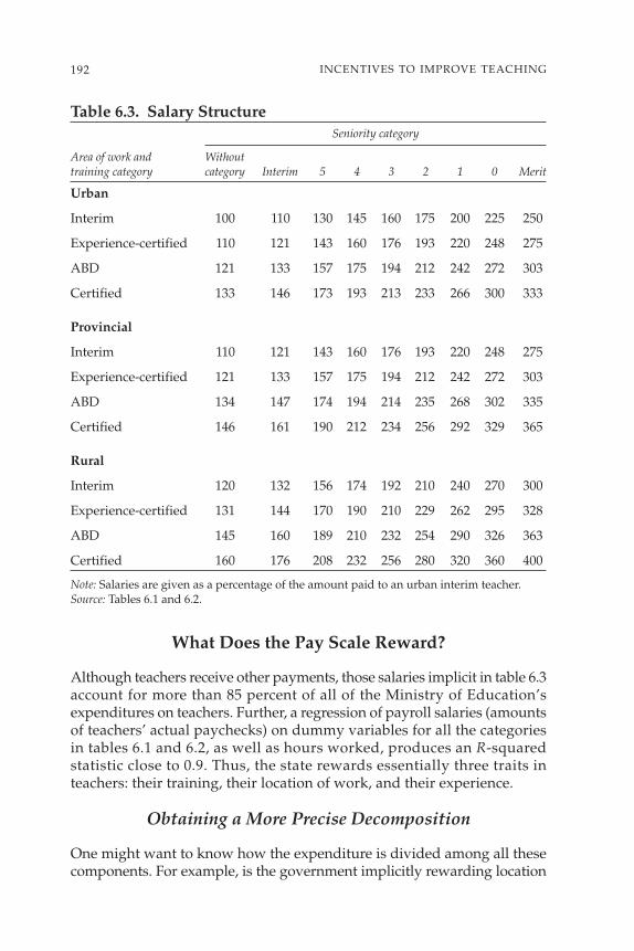
What Does the Pay Scale Reward?
Although teachers receive other payments, those salaries implicit in table 6.3account for more than 85 percent of all of the Ministry of Education’sexpenditures on teachers. Further, a regression of payroll salaries (amountsof teachers’ actual paychecks) on dummy variables for all the categoriesin tables 6.1 and 6.2, as well as hours worked, produces an R-squaredstatistic close to 0.9. Thus, the state rewards essentially three traits inteachers: their training, their location of work, and their experience.
Obtaining a More Precise Decomposition
One might want to know how the expenditure is divided among all thesecomponents. For example, is the government implicitly rewarding location
192 INCENTIVES TO IMPROVE TEACHING
Table 6.3. Salary StructureSeniority category
Area of work and Withouttraining category category Interim 5 4 3 2 1 0 Merit
Urban
Interim 100 110 130 145 160 175 200 225 250
Experience-certified 110 121 143 160 176 193 220 248 275
ABD 121 133 157 175 194 212 242 272 303
Certified 133 146 173 193 213 233 266 300 333
Provincial
Interim 110 121 143 160 176 193 220 248 275
Experience-certified 121 133 157 175 194 212 242 272 303
ABD 134 147 174 194 214 235 268 302 335
Certified 146 161 190 212 234 256 292 329 365
Rural
Interim 120 132 156 174 192 210 240 270 300
Experience-certified 131 144 170 190 210 229 262 295 328
ABD 145 160 189 210 232 254 290 326 363
Certified 160 176 208 232 256 280 320 360 400
Note: Salaries are given as a percentage of the amount paid to an urban interim teacher.Source: Tables 6.1 and 6.2.
of work more than training? In this section, we address this issue in a simpleway. Specifically, we split the salary associated with every possible combi-nation of training, area of work, and seniority (each cell in table 6.3) into fourcomponents: (a) a base payment (in some sense) made simply to put anadult in each classroom, (b) a payment for training, (c) a reward for loca-tion of work, and (d) a payment for experience. We can then add up thecomponents to calculate how much the state spends on each of those traits.
Figure 6.1 illustrates the idea behind this exercise. In it, we focus only onurban areas and, therefore, consider only payments for training and experi-ence (recall that the urban area is the benchmark; teachers receive greaterpay for working outside of it). The figure shows how urban teachers’salaries evolve with experience for each of the four training categories (thatis, it essentially graphs the first panel of table 6.3). As one moves to the right,the steps reflect seniority increases. This graph implicitly assumes, therefore,that teachers move between the Escalafón categories purely on the basis ofexperience. It abstracts from the exams in place since 1994 and from anyother factors that may impede their progress (some of which we discusslater in the chapter). For this reason, the following calculations should beseen as providing an approximation rather than a fully precise accounting.
To see the spirit of the decomposition, consider the highest-paid teacherin this figure: the certified instructor who earns 332.50. What portion ofthis payment is attributable to training and what portion to seniority? Onecan divide the 332.50 into three components as follows:
• A base salary of 100 (the payment to an interim instructor withoutseniority), which is the minimum any teacher receives regardless of hisor her characteristics.
• An additional 150 payment for seniority. This calculation reflects thedifference between 100 and 250, where the latter is the payment made toan interim teacher who is also in the highest experience category. Thus,this payment is made for a teacher’s experience, regardless of his orher training.
• Finally, 82.50 is a reward this teacher receives for training. This figurecomes from the difference between 332.50 and 250, which is the amountpaid to a teacher who is certified, that is, the amount paid over andabove the salary of an interim instructor who has just as many years ofexperience.64
193ARBITRARY VARIATION IN TEACHER SALARIES
64. This calculation might overstate the payment to training and underestimate the pay-ment for seniority somewhat. With experience, interim teachers should eventually becomecertified by experience, although, as we discuss later, this certification does not alwayshappen. In other words, one might expect the two bottom lines in figure 6.1 to merge, butin practice this does not always happen. Thus, we carry out calculations as if it never did.Again, because of the necessity for such simplifying assumptions, our results should beinterpreted as an approximation.

194 INCENTIVES TO IMPROVE TEACHING
0
50
100
150
200
250
300
350
Years of experience
Sala
ry (b
ase
+ “
Esc
alaf
ón”
incr
ease
)
Interim
Experience-certified
ABD
Certified
0 5 10 15 20 25 30 35 40
Figure 6.1. Salary Progression for Urban Teachers of All Training Levels
65. Mechanically, the easiest way of making these calculations is to regress the log ofsalaries on dummies for each of the training, seniority, and location of work categories, wherethe excluded categories are those corresponding to the teacher with the lowest base pay(urban, interim, and no seniority). Not surprisingly, the R-squared statistic on this hypothet-ical decomposition is close to 1. The exponents of the coefficients (in column 2) indicate thepercentage increase over the base salary that accrues to teachers with the associated charac-teristics. For instance, one can see that those for seniority essentially correspond to table 6.2.To obtain the decomposition in table 6.4, we see that the increments implicit in column 2 arethen multiplied by the number of teachers who receive them. For example, the incrementsattributed to provincial and rural status accrue to 36 (each) of the 108 cells in table 6.3. Simi-larly, the increments attributed to the highest seniority accrue to only 12. We then add allthese increments to obtain the decomposition in table 6.4. The results of this exercise are, ofcourse, close to those one obtains doing a manual calculation such as that illustrated usingfigure 6.1.
We carried out a similar calculation for every cell in table 6.3 (for now underthe unrealistic assumption that there is an equal number of teachers in eachcell). Then we aggregated the payments across cells.65
Table 6.4 presents the results of the decomposition for the data intable 6.3. If this were the case, almost half the total wage bill would go tothe base payment (equal to the salary of an urban interim teacher). Of the

remaining half, the majority (about 31 percent) are payments for experi-ence, followed by payments for training (13 percent) and for location ofwork (9 percent).
Factoring in Other Payments
To further flesh out table 6.4, one must consider other payments thatteachers receive. The key additions fall into two categories: bonuses(bonos) and incentive payments. In the first case, two mutually exclusivepayments accrue to some teachers according to their location of work:the Zone and Frontier bonuses. Each of those is equal to 20 percent of theteacher’s base salary. In the first case (Zone), the payment goes to teacherswho work in schools classified as being in inaccessible areas. In the second(Frontier), the payment is for instructors in schools within 50 kilometers ofinternational borders.
Another class of bonus payments, unlike those first two, consists of fixedamounts paid to all qualifying teachers regardless of their base salaries. Thefirst two of those are the Pro-book bonus and the Economic bonus, which in2002 were equal to one monthly minimum wage and 726 bolivianos (Bs.)(about US$100), respectively.
In addition, there is the Attendance bonus, earned by teachers whowork at least 200 days per year. In practice, almost all instructors receive it.Until March 2002, this payment consisted of a lump sum of Bs. 303 peryear (about US$42). As a result of negotiations that ended a 3-week-longstrike, that amount was doubled. None of those amounts enter teachers’base pay; therefore, they do not lead to seniority-related pay increases.
Additionally, at the time of our analysis the Ministry of Education hadthree broadly understood incentive schemes targeted at teachers:
• A payment for teachers who work in and remain in poor, rural regions,called the IPR (Incentivo a la Permanencia en el Area Rural Pobre).
• A payment for teachers who work in bilingual instruction programs,called the IMB (Incentivo a la Modalidad Bilingue).
195ARBITRARY VARIATION IN TEACHER SALARIES
Table 6.4. A Hypothetical Decomposition of the Teacher Wage BillPercentage Category
52.1 Base payment
5.2 Location of work
8.3 Training (preservice)
34.4 Seniority (experience component of the Escalafón)
100.0 Total

• A payment for teachers who engage in certified training, test-takingactivities, or both, called the IAD (Incentivo a la Actualización Docente).
Table 6.5 presents a decomposition that considers all payments. Addition-ally, those results are now weighted to reflect the actual number of teachersin each cell of table 6.3.
Each of the categories in table 6.4 is now broken down into its compo-nents. Base payments cover not only the payments made to an interimteacher in the lowest seniority category, but also the Economic and Pro-book bonuses. Those flat amounts are paid regardless of teachers’ charac-teristics or behavior. Furthermore, the location of work category nowincludes not only the rewards implicit in the Escalafón, but also those thatarise from the Zone, Frontier, and IPR bonuses. Finally, we add an entryfor other behaviors: payments made for traits not rewarded implicitly orexplicitly in the base salary, or Escalafón, calculations.
Despite being purely descriptive, those analyses have several implica-tions. For instance, they reveal that the Ministry of Education spendsabout half of its salary budget in what are essentially lump-sum paymentsto teachers, payments that leave no latitude for rewarding training, expe-rience, or location of work, let alone effort or other behaviors.
196 INCENTIVES TO IMPROVE TEACHING
Table 6.5. A Decomposition of the Teacher Wage BillPercentage Category
47.0 Base payments
40.0 Payments to an urban interim teacher without category4.3 Economic bonus2.5 Pro-book bonus
12.5 Location of work
7.7 Rewards to geography implicit in the Escalafón1.7 Zone bonus2.0 Frontier bonus1.1 IPR (bonus for rural area work)
15.2 Training (preservice)
21.9 Seniority (experience component of the Escalafón)
3.4 Other behaviors
1.0 Administrative bonus0.3 IMB (bonus for bilingual education)2.0 IAD (bonus for in-service training)
100.0 100.0 Total

Additionally, the payments for location of work do not loom large; theyaccount for only about 13 percent of all salary expenditures. Furthermore,the IPR bonus for work in rural areas, which was implemented 2 years ago(and recently abolished), is unlikely to have influenced teachers’ locationchoices very much. Rather, it introduced a marginal change on the overallcompensation pattern. That change accounts for about 1 percent of over-all compensation and only one-tenth of the overall payments for locationof work. Those results also suggest that it might be possible to keep thetotal wage bill constant and yet reduce the base payment while allocatinggreater rewards to encourage teachers to work in rural locations.
Determining whether the allocations in table 6.5 are high or low, or whateffects changing them would have, is beyond the scope of this chapter.Nonetheless, policymakers should find such decompositions useful.
The Flow of Teachers through the Salary Structure
Understanding the movement of teachers through the salary structure isuseful in assessing the structure’s budgetary implications. For this analy-sis, we use the payroll data and limit our analysis to teachers in standard72-hour-per-month positions. This restriction simplifies the analysis, andour sample still accounts for 78 percent of all teaching positions (theremainder of our analyses refer to about 83,000 positions).
Table 6.6 shows the distribution of those teachers by area of work andtraining status. Looking at training status, we see that roughly half theteachers (48 percent) are fully certified. As discussed, ABD teachers oftenhave as much formal preparation as certified instructors, and if we countthem as such, the “trained” share exceeds 75 percent. The remainder ismade up of interim and experience-certified instructors.
197ARBITRARY VARIATION IN TEACHER SALARIES
Table 6.6. Distribution of Teachers by Geographic Region andTraining Status
Location of work
Training status Urban Provincial Rural Totals
Interim 3,144 (3.8) 3,080 (3.7) 9,095 (10.9) 15,319 (18.4)
Experience-certified 1,840 (2.2) 1,031 (1.2) 1,370 (1.6) 4,241 (5.0)
ABD 5,515 (6.6) 6,863 (8.2) 11,902 (14.2) 24,280 (29.0)
Certified 19,930 (23.9) 6,037 (7.2) 13,749 (16.5) 39,716 (47.5)
Totals 30,429 (36.4) 17,011 (20.4) 36,116 (43.2) 83,556 (100.0)
Note: Absolute numbers of department capital are in each category, followed by percentageshares in parentheses.

198 INCENTIVES TO IMPROVE TEACHING
66. The lone position in the fourth category may reflect a coding error.67. At this point they come to be known as interinos inscritos al Escalafón.68. There is one position in the fourth category—again, this might be a coding error.
The data also show a significant variation in the prevalence of trainedinstructors across areas: 16 percent of urban teachers lack formal training,whereas in the provincial and rural areas, 24 and 29 percent, respectively,are in a similar situation. Table 6.6 also shows that about 4 percent of allteachers earn the lowest base salary, while 17 percent earn the highest.
Now consider the distribution according to training and seniority cate-gory, as presented in table 6.7. More than half of the teachers are in the bot-tom three experience categories, largely in the interim and fifth categoryof the Escalafón. This situation is important to keep in mind—it highlightsthat despite the significant returns to experience implicit in the pay struc-ture, more than half of all public school teachers receive relatively smallseniority-related payments. This “bunching up” of teachers at the bottomof the Escalafón has important implications to which we return later.
Note also that there are no teachers in a number of training-experiencecombinations (shaded in gray). For instance, the first column shows thatthe highest seniority category that interim teachers reach is the fifth one.66
As the untrained teachers enter the profession, they go into the interimcategory in the Escalafón, and receive a 10 percent increase over the basesalary (see table 6.2). After 5 years, they can transition into the fifth categoryand receive a 30 percent increase.67 After those 9 years of service, interimteachers can become experience-certified. This transition is visible intable 6.7, where the number of experience-certified teachers jumps from30 to 1,472 between the fifth and the fourth categories, while the numberof interim teachers drops from 2,708 to essentially zero.68
These numbers are also consistent with the presence of high attritionamong the interim teachers. Although the numbers are not sufficient toprove this impression, they are in line with anecdotal evidence suggestingthat eventually many interim teachers find other forms of employment,and very few make it (as experience-certified instructors) into the upperreaches of the Escalafón. This attrition rate may partially reflect that for thefirst 9 years of their careers, those individuals dwell in the lowest-payingparts of the scale.
There are also shaded cells in the column for ABD teachers. In particu-lar, ABD instructors do not progress past the fifth Escalafón category;indeed, being a certified teacher is a requirement for attaining the fourthcategory. This evidence suggests that to the extent some teachers havedifficulties in fulfilling all the certification requirements, a significant num-ber of them get “stuck” in the fifth category—almost one of every fourteachers (not just the ABDs) is in this cell.
The existence of this bottleneck is a key characteristic of the teachercompensation system. Although we do not have direct evidence, the prob-
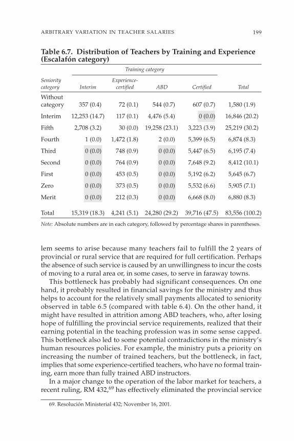
Table 6.7. Distribution of Teachers by Training and Experience(Escalafón category)
Training category
Seniority Experience-category Interim certified ABD Certified Total
Without category 357 (0.4) 72 (0.1) 544 (0.7) 607 (0.7) 1,580 (1.9)
Interim 12,253 (14.7) 117 (0.1) 4,476 (5.4) 0 (0.0) 16,846 (20.2)
Fifth 2,708 (3.2) 30 (0.0) 19,258 (23.1) 3,223 (3.9) 25,219 (30.2)
Fourth 1 (0.0) 1,472 (1.8) 2 (0.0) 5,399 (6.5) 6,874 (8.3)
Third 0 (0.0) 748 (0.9) 0 (0.0) 5,447 (6.5) 6,195 (7.4)
Second 0 (0.0) 764 (0.9) 0 (0.0) 7,648 (9.2) 8,412 (10.1)
First 0 (0.0) 453 (0.5) 0 (0.0) 5,192 (6.2) 5,645 (6.7)
Zero 0 (0.0) 373 (0.5) 0 (0.0) 5,532 (6.6) 5,905 (7.1)
Merit 0 (0.0) 212 (0.3) 0 (0.0) 6,668 (8.0) 6,880 (8.3)
Total 15,319 (18.3) 4,241 (5.1) 24,280 (29.2) 39,716 (47.5) 83,556 (100.2)
Note: Absolute numbers are in each category, followed by percentage shares in parentheses.
lem seems to arise because many teachers fail to fulfill the 2 years ofprovincial or rural service that are required for full certification. Perhapsthe absence of such service is caused by an unwillingness to incur the costsof moving to a rural area or, in some cases, to serve in faraway towns.
This bottleneck has probably had significant consequences. On onehand, it probably resulted in financial savings for the ministry and thushelps to account for the relatively small payments allocated to seniorityobserved in table 6.5 (compared with table 6.4). On the other hand, itmight have resulted in attrition among ABD teachers, who, after losinghope of fulfilling the provincial service requirements, realized that theirearning potential in the teaching profession was in some sense capped.This bottleneck also led to some potential contradictions in the ministry’shuman resources policies. For example, the ministry puts a priority onincreasing the number of trained teachers, but the bottleneck, in fact,implies that some experience-certified teachers, who have no formal train-ing, earn more than fully trained ABD instructors.
In a major change to the operation of the labor market for teachers, arecent ruling, RM 432,69 has effectively eliminated the provincial service
199ARBITRARY VARIATION IN TEACHER SALARIES
69. Resolución Ministerial 432; November 16, 2001.

requirement to become a certified teacher. Because of regular bureaucraticdelays and the number of years it takes to move between Escalafón cate-gories, the effects of RM 432 are only starting to be observed, and the rul-ing’s complete consequences will be evident only after several years.
What effects will it ultimately have? RM 432 is likely to eliminate somecontradictions in the ministry’s compensation policies, as well as to intro-duce others. At a purely financial level, RM 432 will allow large numbersof ABD teachers to become fully certified, which in a few years might placesignificant pressure on the ministry’s budget (this potential outcome doesnot seem to have been carefully analyzed).
At the same time, RM 432 removes what was perhaps the strongestincentive that teachers had for working in the rural area. To the extentthat the ministry is seeking to increase the presence of trained teachers inthe rural area through initiatives like the IPR bonus, these initiatives seemto be contradictory. More specifically, RM 432 seems to remove one of themost powerful (and largely unexploited) policy levers that the ministryhad, because it could have used the eligibility of certain provincial schoolsto direct teachers to relatively poor rural areas (as it tried to do with the IPR).For instance, the ministry could have reclassified schools or announcedthat 1 year of provincial service in particularly poor rural schools wouldbe equivalent to 2 in others. Importantly, such measures could have beenimplemented without modifying any part of the Escalafón, with respect towhich the teacher unions seem to favor the status quo. Those initiativesmight well have been more powerful than incentive payments like the IPR.
Arbitrary Variation in Teacher Salaries
As noted, one source of variation in teacher salaries is the classification ofschools into urban and rural areas, and the concomitant higher compen-sation given to instructors in the latter. A final set of exercises arisesbecause, in practice, the growth of cities has meant that some rural schoolshave been absorbed into an urban setting. One might expect such institu-tions to be reclassified, but given the pay scale, that reclassification wouldamount to lowering the instructors’ salaries. Apparently fearing unionopposition, the Ministry of Education has rarely stripped those schools oftheir rural status. As a result, two teachers with similar training and expe-rience, working in physically very proximate schools, can now earn sig-nificantly different salaries.
Urban Rural Schools
The prevalence of this phenomenon is described in table 6.8 for the threemain districts in the country: La Paz/El Alto, Cochabamba, and Santa
200 INCENTIVES TO IMPROVE TEACHING
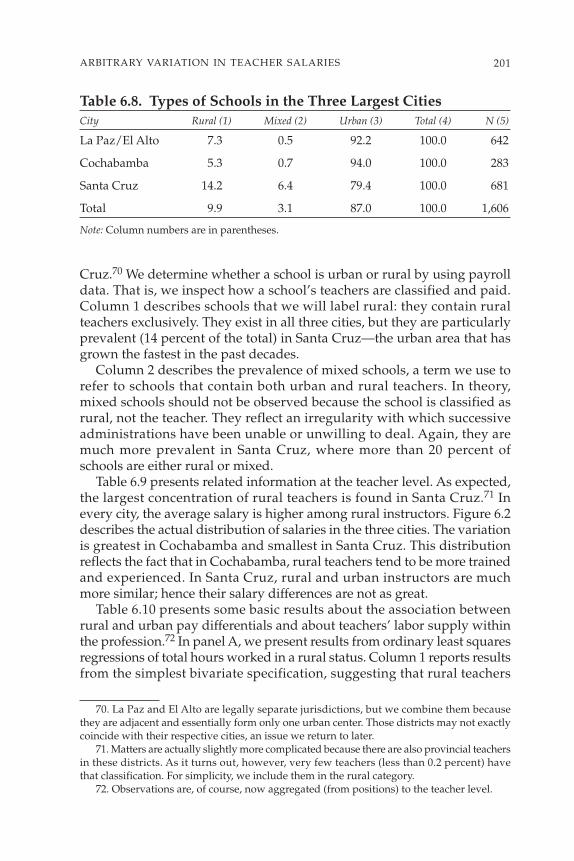
Cruz.70 We determine whether a school is urban or rural by using payrolldata. That is, we inspect how a school’s teachers are classified and paid.Column 1 describes schools that we will label rural: they contain ruralteachers exclusively. They exist in all three cities, but they are particularlyprevalent (14 percent of the total) in Santa Cruz—the urban area that hasgrown the fastest in the past decades.
Column 2 describes the prevalence of mixed schools, a term we use torefer to schools that contain both urban and rural teachers. In theory,mixed schools should not be observed because the school is classified asrural, not the teacher. They reflect an irregularity with which successiveadministrations have been unable or unwilling to deal. Again, they aremuch more prevalent in Santa Cruz, where more than 20 percent ofschools are either rural or mixed.
Table 6.9 presents related information at the teacher level. As expected,the largest concentration of rural teachers is found in Santa Cruz.71 Inevery city, the average salary is higher among rural instructors. Figure 6.2describes the actual distribution of salaries in the three cities. The variationis greatest in Cochabamba and smallest in Santa Cruz. This distributionreflects the fact that in Cochabamba, rural teachers tend to be more trainedand experienced. In Santa Cruz, rural and urban instructors are muchmore similar; hence their salary differences are not as great.
Table 6.10 presents some basic results about the association betweenrural and urban pay differentials and about teachers’ labor supply withinthe profession.72 In panel A, we present results from ordinary least squaresregressions of total hours worked in a rural status. Column 1 reports resultsfrom the simplest bivariate specification, suggesting that rural teachers
201ARBITRARY VARIATION IN TEACHER SALARIES
70. La Paz and El Alto are legally separate jurisdictions, but we combine them becausethey are adjacent and essentially form only one urban center. Those districts may not exactlycoincide with their respective cities, an issue we return to later.
71. Matters are actually slightly more complicated because there are also provincial teachersin these districts. As it turns out, however, very few teachers (less than 0.2 percent) havethat classification. For simplicity, we include them in the rural category.
72. Observations are, of course, now aggregated (from positions) to the teacher level.
Table 6.8. Types of Schools in the Three Largest CitiesCity Rural (1) Mixed (2) Urban (3) Total (4) N (5)
La Paz/El Alto 7.3 0.5 92.2 100.0 642
Cochabamba 5.3 0.7 94.0 100.0 283
Santa Cruz 14.2 6.4 79.4 100.0 681
Total 9.9 3.1 87.0 100.0 1,606
Note: Column numbers are in parentheses.
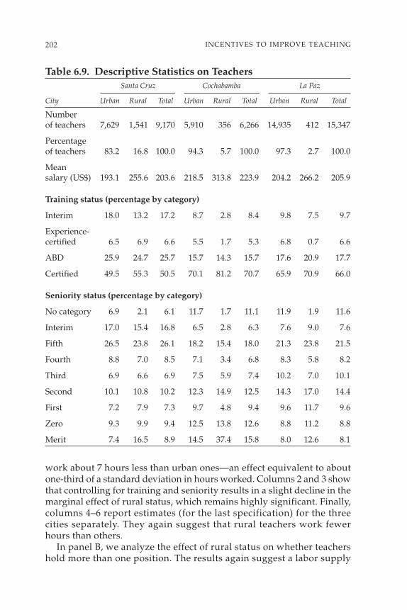
202 INCENTIVES TO IMPROVE TEACHING
Table 6.9. Descriptive Statistics on TeachersSanta Cruz Cochabamba La Paz
City Urban Rural Total Urban Rural Total Urban Rural Total
Numberof teachers 7,629 1,541 9,170 5,910 356 6,266 14,935 412 15,347
Percentage of teachers 83.2 16.8 100.0 94.3 5.7 100.0 97.3 2.7 100.0
Mean salary (US$) 193.1 255.6 203.6 218.5 313.8 223.9 204.2 266.2 205.9
Training status (percentage by category)
Interim 18.0 13.2 17.2 8.7 2.8 8.4 9.8 7.5 9.7
Experience-certified 6.5 6.9 6.6 5.5 1.7 5.3 6.8 0.7 6.6
ABD 25.9 24.7 25.7 15.7 14.3 15.7 17.6 20.9 17.7
Certified 49.5 55.3 50.5 70.1 81.2 70.7 65.9 70.9 66.0
Seniority status (percentage by category)
No category 6.9 2.1 6.1 11.7 1.7 11.1 11.9 1.9 11.6
Interim 17.0 15.4 16.8 6.5 2.8 6.3 7.6 9.0 7.6
Fifth 26.5 23.8 26.1 18.2 15.4 18.0 21.3 23.8 21.5
Fourth 8.8 7.0 8.5 7.1 3.4 6.8 8.3 5.8 8.2
Third 6.9 6.6 6.9 7.5 5.9 7.4 10.2 7.0 10.1
Second 10.1 10.8 10.2 12.3 14.9 12.5 14.3 17.0 14.4
First 7.2 7.9 7.3 9.7 4.8 9.4 9.6 11.7 9.6
Zero 9.3 9.9 9.4 12.5 13.8 12.6 8.8 11.2 8.8
Merit 7.4 16.5 8.9 14.5 37.4 15.8 8.0 12.6 8.1
work about 7 hours less than urban ones—an effect equivalent to aboutone-third of a standard deviation in hours worked. Columns 2 and 3 showthat controlling for training and seniority results in a slight decline in themarginal effect of rural status, which remains highly significant. Finally,columns 4–6 report estimates (for the last specification) for the threecities separately. They again suggest that rural teachers work fewerhours than others.
In panel B, we analyze the effect of rural status on whether teachershold more than one position. The results again suggest a labor supply

203ARBITRARY VARIATION IN TEACHER SALARIES
0100 200 300 400
Relative salary
La Paz/El Alto
rural
urban
0100 200 300 400
Relative salary
Cochabamba
rural
urban
0100 200 300 400
Relative salary
Santa Cruz
rural
urban
Figure 6.2. Distributions of Relative Salaries for Urban and Rural Teachers

204IN
CE
NT
IVE
ST
OIM
PR
OV
ET
EA
CH
ING
Table 6.10. Hours Worked and the Probability of Holding a Second Teaching JobAll cities
La Paz/El Alto Cochabamba Santa Cruz(1) (2) (3) (4) (5) (6)
Panel A. Dependent variable = Total hours worked
Rural status –7.2*** –7.3*** –4.2*** –6.9*** –6.0*** –3.7***(0.5) (0.5) (0.4) (0.8) (0.9) (0.6)
[−0.35] [−0.36] [−0.21] [−0.34] [−0.30] [−0.18]
Controls: Teacher and school characteristics No Yes Yes Yes Yes Yes
Dummies for experience categories No No Yes Yes Yes Yes
N 24,973 24,973 24,973 12,230 4,719 8,024
R2 0.010 0.018 0.342 0.411 0.401 0.220
Panel B. Dependent variable = Dummy for holding more than one job (linear probability)
Rural status –0.16*** –0.16*** –0.09*** –0.10*** –0.16*** –0.06***(0.01) (0.01) (0.01) (0.02) (0.02) (0.01)
Dummies for training categories No Yes Yes Yes Yes Yes
Dummies for experience categories No No Yes Yes Yes Yes
N 24,973 24,973 24,973 12,230 4,719 8,024
R2 0.013 0.015 0.408 0.470 0.357 0.302
Note: Column numbers are in parentheses in the column heads. *** indicates significance at the 1 percent level. Huber-white standard errors are inparentheses. Brackets contain the proportion of a standard deviation change in the dependent variable.

205ARBITRARY VARIATION IN TEACHER SALARIES
effect: having rural status is associated with a reduction of about 15 per-cent in the probability that the teacher has a second teaching position. Thisconclusion is robust to the addition of training and experience controls,and to the estimation within cities.73
There are several things to note when interpreting the results. First,although it seems clear that rural teachers work less, we are unable to ascer-tain the mechanism behind this finding. In a conventional interpretation,one might think that having rural status and, hence, enjoying higher earn-ings would induce substitution and income effects on labor supply, andthat the latter would dominate. In some sense, this assumption might notbe shocking, given that, as elsewhere, a significant proportion of Bolivianteachers seem to be mothers and secondary earners who express a prefer-ence for spending part of the day at home (Urquiola and others 2000).
Such an inference, however, requires an assumption that the individu-als who select into rural schools are not systematically different from thosein urban institutions, so that any differences in the hours or the numberof positions they work might plausibly be caused by variations in theirpay. This assumption is strong, given that into the mid-1990s the route intothe two types of schools was somewhat different. Specifically, in the past,urban and rural teachers were trained in different institutions and belongedto different unions.
Furthermore, to the extent that attaining rural status might require“gaming the system” (for example, the existence of mixed schools whenthey should not occur), then teachers who attain such positions might bedifferent from others in unobserved ways. Another concern arises if it isadministratively harder for rural teachers to increase either their hours orthe number of positions they teach in, because, presumably, there is higherdemand for those higher-paying posts. Finally, we note that our resultsoriginate in administrative data that capture only teachers’ labor supplywithin the profession. The data do not tell us whether rural teachers might beengaging any more or less in outside activities, such as driving a cab.
Urban and Rural Pay Differentials and Achievement
A related question is whether rural teachers, perhaps because they arepaid more, exert more effort and thus produce better outcomes. Again,using the urban and rural pay differences to address this issue requires sig-nificant assumptions. First, urban and rural teachers in these cities ideallyshould be similar except for their rural or urban status. In some of the fol-lowing analyses, we focus on Santa Cruz; although the variation in teacher
73. Logit regression results, which we omit, yield qualitatively similar conclusions.
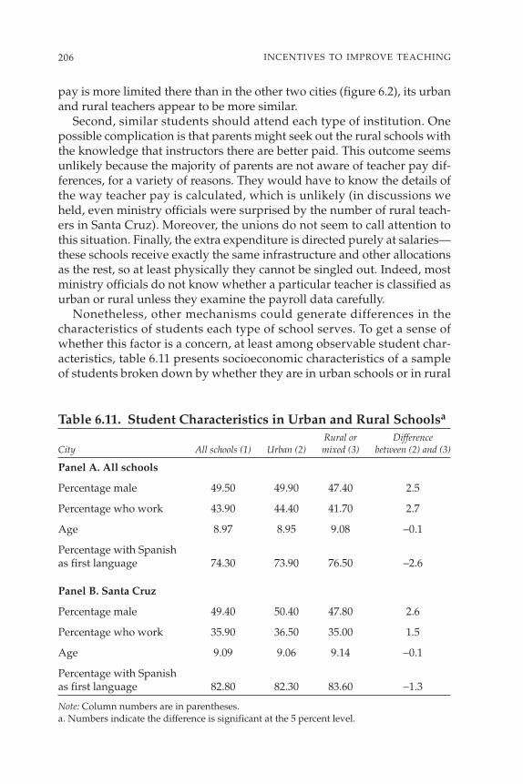
pay is more limited there than in the other two cities (figure 6.2), its urbanand rural teachers appear to be more similar.
Second, similar students should attend each type of institution. Onepossible complication is that parents might seek out the rural schools withthe knowledge that instructors there are better paid. This outcome seemsunlikely because the majority of parents are not aware of teacher pay dif-ferences, for a variety of reasons. They would have to know the details ofthe way teacher pay is calculated, which is unlikely (in discussions weheld, even ministry officials were surprised by the number of rural teach-ers in Santa Cruz). Moreover, the unions do not seem to call attention tothis situation. Finally, the extra expenditure is directed purely at salaries—these schools receive exactly the same infrastructure and other allocationsas the rest, so at least physically they cannot be singled out. Indeed, mostministry officials do not know whether a particular teacher is classified asurban or rural unless they examine the payroll data carefully.
Nonetheless, other mechanisms could generate differences in thecharacteristics of students each type of school serves. To get a sense ofwhether this factor is a concern, at least among observable student char-acteristics, table 6.11 presents socioeconomic characteristics of a sampleof students broken down by whether they are in urban schools or in rural
206 INCENTIVES TO IMPROVE TEACHING
Table 6.11. Student Characteristics in Urban and Rural Schoolsa
Rural or Difference City All schools (1) Urban (2) mixed (3) between (2) and (3)
Panel A. All schools
Percentage male 49.50 49.90 47.40 2.5
Percentage who work 43.90 44.40 41.70 2.7
Age 8.97 8.95 9.08 −0.1
Percentage with Spanish as first language 74.30 73.90 76.50 −2.6
Panel B. Santa Cruz
Percentage male 49.40 50.40 47.80 2.6
Percentage who work 35.90 36.50 35.00 1.5
Age 9.09 9.06 9.14 −0.1
Percentage with Spanish as first language 82.80 82.30 83.60 −1.3
Note: Column numbers are in parentheses.a. Numbers indicate the difference is significant at the 5 percent level.

and mixed schools. These variables are drawn from a student question-naire administered to students along with the standardized examinations.They include the student’s gender, age, whether she or he works outsideof school, and whether Spanish is his or her native language. As the tableshows, for none of these variables is the difference across types of schoolsstatistically significant.
Table 6.12 presents results on whether student outcomes vary acrossthese two sectors. Panels A and B refer to language and math test scores
207ARBITRARY VARIATION IN TEACHER SALARIES
Table 6.12. Hours Worked by Teachers and Probability ofHolding a Second Job
All cities Santa Cruz
(1) (2) (3) (4)
Panel A. Average third-grade language score
Rural status −0.10 −0.11 0.03 0.08(0.12) (0.12) (0.18) (0.19)
[−0.10] [−0.11] [0.03] [0.08]
Controls: Teacher and school characteristics No Yes No Yes
N 698 698 225 225
R2 0.001 0.009 0.000 0.021
Panel B. Average third-grade math score
Rural status 0.06 0.09 0.15 0.27(0.12) (0.12) (0.20) (0.21)[0.12] [0.12] [0.20] [0.21]
Controls: Teacher and school characteristics No Yes No Yes
N 698 698 225 225
R2 0.000 0.005 0.002 0.041
Panel C. Repetition rate
Rural status −0.006** −0.004 −0.000 −0.000(0.003) (0.003) (0.004) (0.004)[−0.13] [0.09] [−0.00] [−0.00]
Controls: Teacher and school characteristics No Yes No Yes
N 1,220 1,220 477 477
R2 0.003 0.043 0.000 0.007(Continued)

208 INCENTIVES TO IMPROVE TEACHING
Table 6.12. Hours Worked by Teachers and Probability ofHolding a Second Job (Continued)
All cities Santa Cruz
(1) (2) (3) (4)
Panel D. Pass rate
Rural status 0.014*** 0.00*** 0.010** 0.009**(0.004) (0.004) (0.005) (0.00)[0.28] [0.24] [0.20] [0.18]
Controls: Teacher and school characteristics No Yes No Yes
N 1,187 1,187 467 467
R2 0.010 0.044 0.010 0.024
Panel E. Dropout rate
Rural status 0.009*** 0.006*** 0.004 0.003(0.001) (0.001) (0.001) (0.001)[0.56] [0.38] [0.25] [0.19]
Controls: Teacher and school characteristics No Yes No Yes
N 975 975 412 412
R2 0.055 0.340 0.018 0.276
Note: Column numbers are in parentheses in the column heads. **, *** indicate significanceat the 5 and 1 percent level, respectively. Huber-white standard errors are in parentheses.Brackets contain the proportion of a standard deviation change in the dependent variable.
and contain no significant evidence that scores are significantly differentbetween rural and urban schools. Columns 1 and 2 present pooled resultsfor schools in all three cities, and columns 3 and 4 refer to Santa Cruz only.
The results in panels C–E draw on administrative data to examine towhat extent repetition, pass, or dropout rates differ across the two types ofschools. We find some contradictory evidence. Rural schools appear tohave lower repetition and higher pass rates, but also higher dropoutrates—although those results are not always significant. The bottom lineis that, given the strong assumptions required and the weak results, wecannot draw substantial conclusions from our regressions.
In an attempt to identify better comparison groups for this analysis,we collected GIS information on the location of all schools in Santa Cruz.Figure 6.3 presents those data; the dots represent urban schools, and thetriangles stand for rural institutions. We carried out analyses by using

comparison groups for each rural school and by selecting the urbanschools closest to that school (for example, within a certain radius). Thelogic behind this method is that, to the extent schools serve neighborhoodhouseholds, the surrounding schools might provide better comparisongroups. We again do not find consistent evidence of performance differ-ences for urban and rural schools using this classification criterion.
In short, we find no systematic differences in achievement betweenurban and rural schools. Although this result may be because our empiri-cal strategies do not successfully identify those differences, it leaves openthe possibility that the extra expenditure in this area is not really buyingbetter outcomes.
209ARBITRARY VARIATION IN TEACHER SALARIES
= Urban schools= Rural schools
Figure 6.3. GIS Data for Santa Cruz Schools

210 INCENTIVES TO IMPROVE TEACHING
Conclusions
In many developing countries, the teacher wage bill accounts for the vastmajority of recurrent educational expenditures. Additionally, teacher payscales are frequently fairly rigid and have features that governments findpolitically very costly to change. In such contexts, it is important to under-stand well the details of the pay scheme. What is the state implicitly pay-ing for and obtaining? What implicit and explicit incentives does the payscale contain?
In this chapter, we have addressed such questions for Bolivia. We haveprovided a detailed characterization of teacher compensation and of theteacher traits—training, location of work, and experience—that the salarystructure seems to reward. Additionally, we analyzed the flow of teachersthrough the pay scale, highlighting budgetary implications and potentialcontradictions in the ministry’s human resources policy. Finally, weattempted to determine whether the arbitrary variation in teacher salariesthat the pay scale generates in some cities has any effect on teachers orstudent outcomes (as measured by standardized test scores). Although ourfindings indicate that the rural and urban teacher pay differential is asso-ciated with a variation in the labor supply for teachers, we do not findany systematic relation with student achievement.
All of our conclusions are, of course, specific to Bolivia. Nonetheless, theexercises we present may provide a useful template for analyses in otherdeveloping countries that also have fairly centralized and rigid teachercompensation schemes.

References
Ballou, D., and M. Podgursky. 1997. Teacher Pay and Teacher Quality.Kalamazoo, Mich.: W. E. Upjohn Institute for Employment Research.
Lankford, H., and J. Wycoff. 1997. “The Changing Structure of TeacherCompensation, 1970–94.” Economics of Education Review 16(4): 371–84.
Liang, X. 1999. “Teacher Pay in 12 Latin American Countries: How DoesTeacher Pay Compare to Other Professions, What Determines TeacherPay, and Who Are the Teachers?” Latin America and the CaribbeanRegion Human Development Department Paper 49. World Bank,Washington, D.C.
Mizala, A., and P. Romaguera. 2001. “Are Teachers Underpaid? Evidencefrom Chile.” Center for Applied Economics, Department of IndustrialEngineering, University of Chile, Santiago. Processed.
Morduchowicz, A. 2002. Carreras, incentivos y estructura salariales, docentes.Buenos Aires: Programa de Reforma Educativa en América Latina.
Piras, C., and W. Savedoff. 1998. “How Much Do Teachers Earn?” IDB Work-ing Paper 375. Inter-American Development Bank, Washington, D.C.
Podgursky, M. 2000. “The Relative Pay and Contractual Work Hours ofNew York City Teachers.” Department of Economics, University ofMissouri–Columbia. Processed.
Urquiola, M., W. Jiménez, M. L. Talavera, and W. Hernany. 2000. Los mae-stros en Bolivia: Impacto, incentivos y desempeño. La Paz: Sierpe.
Vegas, E., L. Pritchett, and W. Experton. 1999. “Attracting and RetainingQualified Teachers in Argentina: Impact of the Level and Structure ofCompensation.” Latin America and the Caribbean Region HumanDevelopment Department Paper 38. World Bank, Department ofHuman Development, Latin America and the Caribbean RegionalOffice, Washington, D.C.
211


7Teacher and Principal Incentives in Mexico
Patrick J. McEwanWellesley College
and Lucrecia SantibáñezRAND Corporation
Across the world, teacher pay is overwhelmingly determined by teachers’levels of education and years of experience. There is mounting concern thatrigid compensation structures weaken teachers’ incentives to exert effortand to improve student performance. In the United States and elsewhere,such concerns have led to the use of monetary performance incentives,often based on the level or growth of students’ test scores. Nonetheless, payfor performance is relatively rare, and existing plans are often small scaleand short lived.74
In contrast, since 1993, Mexican public school teachers and principalshave been eligible for large financial awards that are based on students’ testscores, among other factors. Under the Carrera Magisterial program,75
personnel voluntarily participate in a year-long assessment process thatawards 100 points for education, experience, students’ test scores, and otherfactors. In recent years, personnel scoring above a nationally specified cut-off score (70) have a sharply higher probability of receiving an award. Theawards are substantial, and they persist for the teacher’s entire career.
213
We would like to thank Felipe Martínez Rizo and Alfredo González V. from InstitutoNacional para la Evaluación Educativa (INEE) for supplying data and replying to manyinquiries. Victor Sastré from Carrera Magisterial was also very helpful in answering our ques-tions. The research received financial support from the World Bank, Wellesley College, andRAND. Those individuals and institutions are not responsible for any errors or interpreta-tions. Patrick J. McEwan can be contacted at [email protected]. Lucrecia Santibáñezcan be contacted at [email protected].
74. Only nine U.S. states have laws that encourage such policies (Education Week 2004).On the short-lived nature of early merit pay plans, see Murnane and Cohen (1986). For recentreviews, see Glewwe, Ilias, and Kremer (2003) and Lavy (2002).
75. Carrera Magisterial roughly translates into English as Teachers’ Career Ladder.

This chapter examines whether the incentives provided by CarreraMagisterial have induced teachers and principals to improve students’ testscores.76 One avenue by which improvements could have occurred wasincreased effort, although the recent literature on accountability hasemphasized that a variety of gaming behaviors could also produceimprovements in test scores.77 In either case, the essential challenge is tocompare a group of personnel who are receiving incentives—or rather,their students’ outcomes—to a reasonable counterfactual.78 At first glance,there is no obvious counterfactual against which to gauge the program’seffects on students’ test scores. The Mexican data were collected for theadministrative purpose of allocating rewards. As such, they includeobservations on only those teachers and principals who are putatively con-sidered to receive incentives and who participated in the assessmentprocess (our first group).
This chapter argues that many teachers and principals within theCarrera Magisterial program (our second group) faced weak incentivesand that these educators provide useful counterfactuals. Among teachers,for example, 80 points are determined by background characteristics (suchas education and experience) and by a teacher’s test score. Those pointsare determined before the students’ tests, which account for the remaining20 points, are administered. A significant number of teachers obtained sofew points from their background characteristics that even perfectly scor-ing students would not place them above the cutoff. Other teachers scoredabove the cutoff even without the additional points from students’ testscores. Both groups of teachers had little incentive to exert much effort toraise their students’ test scores.
214 INCENTIVES TO IMPROVE TEACHING
76. Because the Carrera Magisterial reform is so far reaching, it resembles an across-the-board wage increase for personnel. Thus, a substantial effect might be that the quality ofentering cohorts of teachers has increased in the past decade. In the United States, Figlio(2002) examines whether higher teacher salaries attracted high-quality new teachers.
77. We will remain agnostic about the exact mechanisms by which such an improvementmight occur. One possibility is that teachers exert greater effort in the classroom over thecourse of the school year. Others are that cheating occurs (see Jacob and Levitt 2003); that low-achieving students are excluded from high-stakes testing (see, for example, Cullen andReback 2002; Figlio and Getzler 2002); that students receive coaching on test-taking (see, forexample, Glewwe, Ilias, and Kremer 2003); or even that schools increase students’ caloricintake on the day of the test (see Figlio and Winicki forthcoming). For a recent overview ofthis literature, see Hanushek and Raymond (2002).
78. A small body of literature has applied experimental and quasi-experimentalapproaches. In a recent evaluation of a pilot teacher incentive scheme in Kenya, incentiveswere allocated to 50 schools, which were randomly selected from a group of 100 (Glewwe,Ilias, and Kremer 2003). Lavy (2002) examined a small-scale program in Israel that providedincentives to teachers in 62 secondary schools. He used a regression-discontinuity approachto compare student outcomes in the 62 schools to those of schools that just missed treatmentbecause of eligibility rules.
A third group of teachers face a stronger incentive to improve studenttest scores, because they are close to—but not assured of—receiving anaward.79 We argue that the nonlinear structure of the awards introduces adiscontinuity in the relationship between a teacher’s initial point score(excluding points from students’ test scores) and his or her classroom testscore. Our initial focus is on testing for existence of such as a discontinuity,which could be plausibly attributed to a program-induced improvementin test scores.
As an additional empirical strategy, we note that many teachers’ proba-bilities of being promoted—even when conditional on scoring above thenational cutoff—are not the same across Mexico’s 32 states. (Each state isresponsible for allocating promotions.) In some states, teachers scoringabove the cutoff have lower promotion probabilities. We argue that suchteachers perceive the expected value of the monetary award to be lower.Hence, they face relatively weaker incentives than teachers working in stateswith a higher probability. We use teachers in lower-probability states as acounterfactual for other teachers in a difference-in-differences framework.
In addition to analyzing incentives for teachers, we consider those forprincipals.80 Principals are subject to the same annual evaluations as teach-ers, but instead of the students’ test score, they receive a school perfor-mance score, which reflects the student performance score for participatingteachers, as well as teachers’ test scores. We use empirical strategies simi-lar to the ones previously described for teachers to analyze whether theincentives offered by Carrera Magisterial to school principals had any effecton school performance.
215TEACHER AND PRINCIPAL INCENTIVES IN MEXICO
79. A related phenomenon has been noted in other pay-for-performance systems inwhich awards are a nonlinear function of a performance measure, such as fixed sales quotas(for a review, see Prendergast 1999). Prendergast (1999, p. 26) notes that “an agent who isclose to winning the prize will have greater incentive . . . than one who has either exceededthe quota or is unlikely to reach that quota.” Courty and Marschke (2004) provide recentevidence of such incentives—and the gaming response of participants—in the national JobTraining Partnership Act program, in which bonuses received by local job training centerswere a nonlinear function of their graduation rates.
80. Research on school effectiveness has shown that school principals play a key role inimproving schools. For example, see Zigarelli’s (1996) review on school effectiveness. It citesthe leadership and involvement of principals as one of the three constructs that define schooleffectiveness. Other researchers who argue that principals play a key role in school effective-ness are Bossert and others (1982), Eberts and Stone (1988), and Hallinger and Murphy (1986).However, incentive programs for school principals are extremely rare. In Mexico, schoolprincipals are unionized and are subject to uniform salary schedules in the same way thatteachers are. In the United States and other countries, principals in larger or otherwisemore difficult schools receive higher salaries (Gates and others 2003). However, school prin-cipals in Mexico who work in very large urban schools will receive almost the same com-pensation as those in very small, suburban schools. Mexican principals, therefore, have verylittle incentive to perform outside their assigned duties under this uniform structure.

The empirical analysis for teachers and principals, relying on bothcounterfactuals, does not provide strong, robust evidence that personnelimprove their outcomes when they face stronger incentives. The discus-sion explores several possible reasons for this finding. The next sectionprovides institutional background on the Carrera Magisterial program.
The Carrera Magisterial Program
Carrera Magisterial was instituted in January 1993 as one component of alarge education reform known as the National Agreement for the Mod-ernization of Basic Education.81 Before the reform, teacher and schooladministrator pay was determined by levels of education and years ofexperience. Since the reform, teachers and principals are eligible for sub-stantial and permanent wage increases if they perform well in a year-longassessment process that emphasizes many factors, including students’ testscores or school performance. Teachers and principals consent to theassessment process in October, near the beginning of the school year. Theprocess is voluntary, but the vast majority of Mexico’s eligible teachers andprincipals have participated.82 Personnel are evaluated in six areas and areawarded points in each. These areas are (a) education degrees; (b) yearsof experience; (c) professional development, including federal and state in-service training courses; (d) peer review; (e) teacher (or principal) knowl-edge, which is based on a test score; and (f) student performance, whichis based on students’ test scores.
Table 7.1 describes the points that are currently awarded for each factor,summing to 100 points.83 The assessment process places substantial weighton individuals’ formal education and experience, awarding up to 25 pointsfor those two areas. Another 17 points is awarded for participation in shorttraining courses offered by the federal or state governments, and 28 points
216 INCENTIVES TO IMPROVE TEACHING
81. Besides Carrera Magisterial, the reform instituted a massive administrative decen-tralization of Mexico’s public schools from the nation to its 32 states, as well as revised cur-ricula and textbooks. For details, see Presidency of the Republic of Mexico (1992). The CarreraMagisterial program is jointly managed by the Ministry of Education (Secretaría de EducaciónPública, or SEP) and the teachers’ union, Sindicato Nacional de Trabajadores de la Educación(National Education Workers’ Union, or SNTE).
82. To be eligible, teachers must belong to the SNTE and must meet a minimum senior-ity requirement that varies by education degree. In addition, both teachers and principalsmust hold specific kinds of contracts with SEP (such as a permanent teaching position, orplaza, which is roughly analogous to a tenured position in the United States, or a contractposition that can be renewed indefinitely, which is called interinato ilimitado).
83. The program has experienced a number of administrative modifications during thepast 10 years, including the weighting of the factors. We will argue that the program’s fea-tures before its ninth year (the 1999/2000 academic year) complicate our efforts to crediblyidentify its effect. Hence, the following discussion and empirical analysis will focus on thelater years of the program.

are awarded for a teacher (or principal) knowledge test that is administeredin early March (SEP n.d.). Also, 10 points are awarded for supervisorreview, in which principals rate teachers’ performance and inspectors rateprincipals’ performance. This element has little variation, because mostteachers and principals receive very high ratings. Finally, the unadjustedmean test score of a teacher’s students is worth 20 points.84 The students’tests are administered at the end of the school year, in mid-June (SEP n.d.).Principals receive 20 points that are based on school performance, whichis a composite of the teacher-specific scores of the participating teachers inthe principal’s school. These 20 points are made up of up to 10 points forthe average of teachers’ knowledge scores in the school and up to 10 pointsfor the average of students’ test scores in the school.
There are five levels of promotion in Carrera Magisterial, denoted A,B, C, D, and E. Each level represents a successively larger wage bonus.The levels must be pursued sequentially, beginning with level A.85 Oncepromoted to a given level, individuals cannot be demoted, and their
217TEACHER AND PRINCIPAL INCENTIVES IN MEXICO
Table 7.1. Evaluation Scheme for Carrera MagisterialTeachers’ Principals’
Factor maximum points maximum points
Education 10 10
Experience 15 15
Supervisor evaluation 10 10
Federal in-service training courses 12 12
State in-service training courses 5 5
Professional knowledge:Teacher test score 28Principal test score 28
Performance:Classroom test scores 20School average scores 20
Total 100 100
Source: National Coordinating Committee of Carrera Magisterial.
84. Some teachers are given a small bonus in this factor (up to 4 points) as an ad hoccompensation for working with students with disabilities or for having students place in thetop positions in various regional and national competitions.
85. In the initial years of the program, some teachers skipped level A and were promotedautomatically to levels B and upward. This possibility was eliminated in the eighth year ofthe program.

wage bonus remains constant throughout their careers. They must waitfor a specified number of years before they can attempt promotion tohigher levels.86 The wage bonuses for participants are substantial, con-sisting of a percentage of the base wage (determined from a standardwage schedule that emphasizes education and experience). In recentyears, level A teachers receive 24.5 percent of their base wage, whereaslevel E teachers receive 197 percent (Ortiz Jiménez 2003). The bonuses arelarge when compared with those available under teacher incentive plansin other countries, particularly given that they are not simply one-timepayments.87
Promotion opportunities are determined by each participant’s final pointscore, which is calculated by the national office of Carrera Magisterial. Thefinal point totals are distributed through an electronic spreadsheet to eachof Mexico’s 32 state-level offices, where the final selection is conducted.In the early years of the program, states were given much leeway in deter-mining the cutoff score above which teachers and principals were pro-moted. Hence, the cutoffs apparently varied by state and, from year toyear, within states. Since the program’s ninth year (the 1999/2000 schoolyear), each state has been constrained by a well-publicized national cut-off score (Ortiz Jiménez 2003).88 No individual scoring below 70 points iseligible for promotion to levels A–E. Our evidence suggests that statesoverwhelmingly complied with this rule. Individuals scoring above 70comprise the eligible pool of participants in each state, although not allof those scoring above the cutoff are actually awarded promotion. We willexplore the possible determinants of promotion among high-scoringteachers in later sections.
Since 1992, the program has promoted a large number of Mexicanteachers and principals (see tables 7.2 and 7.3). Close to 600,000 preschool,
218 INCENTIVES TO IMPROVE TEACHING
86. Participants in levels A and B must wait 3 years before they are eligible for a promo-tion to the next level. If they work in specified poor areas, they must wait only 2 years. Thosein levels C and D must wait 4 years before being eligible for a promotion. That timeframe islowered to 2 years for individuals working in poor areas. Teachers and principals can par-ticipate in the assessment process each year while they are waiting to become eligible and canchoose the highest score to use for their promotion.
87. For example, Glewwe, Ilias, and Kremer (2003) note that incentive plans in the UnitedStates typically offer one-time payments of 10 to 40 percent of the monthly wage. Israel hasoffered payments of 60 to 300 percent of the monthly wage, but they were still only one-time payments (Lavy 2002).
88. Up until the program’s eighth-year, there appeared to be few rigid rules governingeach state’s approach to allocating the awards. Each state was provided a yearly budget thatconstrained the number of promotions that could be awarded. Once the number of promo-tions was determined, most states apparently relied heavily on the final point score to allo-cate rewards. However, it is not clear whether states adhered to a deterministic cutoff (that is,all teachers scoring above a given point value would receive a promotion).

primary, and secondary teachers and about 85,000 principals have beenpromoted to level A, although fewer promotions have been awarded inrecent years because the pool of eligible participants is declining.89
Data
In each year since the program’s inception, the national office of CarreraMagisterial has collected data used in the assessment process describedabove. This chapter uses data from recent years (years 9–11) of the pro-gram. We do so principally because the program began relying on asharp, national assignment cutoff in year 9. The sample of teachers islimited to primary teachers in grades 3–6, because teachers in grades 1–2did not participate in the student assessment. The sample of principals is
219TEACHER AND PRINCIPAL INCENTIVES IN MEXICO
Table 7.2. Teacher Promotions in Carrera MagisterialPromotions Promotions Percentage of
Program to level A to level A teachers promoted year School year (in that year) (cumulative) Total teachers (cumulative/total)
1 and 2 1991/92 315,773 315,773 764,796 41and 1992/93
3 1993/94 87,743 403,516 785,023 51
4 1994/95 58,391 461,907 812,358 57
5 1995/96 40,066 501,973 831,573 60
6 1996/97 32,033 534,006 858,054 62
7 1997/98 26,518 560,524 869,632 64
8 1998/99 10,468 570,992 888,126 64
9 1999/2000 9,210 580,202 896,917 65
10 2000/01 8,964 589,166 910,919 65
11 2001/02 6,808 595,974 921,588 65
Notes: The total for teachers includes preschool, primary, and secondary teachers in publicschools. Carrera Magisterial promotion figures are for the teacher program category only(primera vertiente). Promotions refer to a teacher entering level A of the program for thefirst time.Source: Secretaría de Educación Pública (http://www.sep.gob.mx) and Ortiz Jiménez (2003).
89. Over half of the promotions occurred in the first 2 years of the program. It should benoted that these initial promotions occurred automatically—a diplomatic way of saying thatthe assessment process was not fully functional until the third year; thus, all applicants werepromoted. As a result, the first 2 years of the program amounted to an across-the-board wageincrease for many teachers and principals.

limited to primary school principals. Finally, in both cases, the sampleincludes only participants seeking promotion to level A.
Table 7.4 reports descriptive statistics on the teacher sample. The sam-ple contained 76,567 teacher observations in 27,213 schools.90 The vari-ables include the same ones used to construct each teacher’s final score(see table 7.1). Note that a relatively small percentage of the sample (3 percent) received a final score above 70; we will corroborate that amajority of those teachers were the same ones promoted to level A. Thedata include a small number of other variables that we will use as controls,including the teacher’s gender, the grade level of instruction, and the ses-sion of instruction. (Most Mexican primary classes are taught in a morning
220 INCENTIVES TO IMPROVE TEACHING
Table 7.3. Principal Promotions in Carrera MagisterialPromotions Promotions Percentage of
Program to level A to level A Total principals promoted year School year (in that year) (cumulative) principals (cumulative/total)
1 and 2 1991/92 52,565 52,565 76,724 69and 1992/93
3 1993/94 14,606 67,171 78,544 86
4 1994/95 5,479 72,650 82,671 88
5 1995/96 3,333 75,983 85,360 89
6 1996/97 2,105 78,088 86,270 91
7 1997/98 2,017 80,105 87,864 91
8 1998/99 553 80,658 89,161 90
9 1999/2000 520 81,178 88,457 92
10 2000/01 2,224 83,402 89,107 94
11 2001/02 1,420 84,822 89,307 95
Notes: The number of total primary school principals in the system is estimated from SEP(2003). It is estimated by taking the total number of public and private primary schools andmultiplying by 90 percent (the assumed proportion of public primary schools). The calculationassumes that there is one principal per school; hence, the number of schools represents thenumber of principals. Carrera Magisterial promotion figures are for the principal programcategory only (segunda vertiente). Promotions refer to principals entering level A of the programfor the first time. Principals who were later promoted into levels B–E would still be included inthe cumulative level A figure. In years 1–7, some principals were promoted directly to levels Band higher; this provision was later eliminated. Figures for year 11 are estimated.Source: SEP (2003); Carrera Magisterial (Estadística Básica Etapas 3–10 available athttp://www.sep.gob.mx); and Ortiz Jiménez (2003).
90. Mexican teachers can hold positions in more than one school. In a given year, there-fore, some teachers are observed more than once. The same is true for school principals.

221TEACHER AND PRINCIPAL INCENTIVES IN MEXICO
Table 7.4. Descriptive Statistics for TeachersVariable Mean Minimum Maximum Description
Education 7.94 0 15 Points awarded for educational (2.24) degrees
Experience 5.31 0 10 Points awarded for years of (2.65) experience
Peer review 9.17 0 10 Points awarded for peer (1.06) review by teacher colleagues
Federal 1.19 0 12 Points awarded for participation training (2.85) in federal-level training courses
State 3.01 0 5 Points awarded for participationtraining (2.39) in state-level training courses
Teacher 15.18 0 28 Points awarded for teacher test (3.89) knowledge test
Disability 0.04 0 4 Additional points awarded to (0.36) teachers whose students have
disabilities
Initial points 41.84 5 75.45 Sum of the 7 previous variables
Initial points < 50 0.85 0 1
Initial points 50–70 0.15 0 1
Initial points ≥ 70 < 0.01 0 1
Test score 10.77 0.25 20 Points awarded for mean score (2.78) of students in classroom
Final points 52.61 16.81 88.84 Sum of initial points and test (8.71) score
Final points ≥ 70 0.03 0 1
Promoted 0.03 0 1 Promoted to level A
Attempts 3.23 1 10 Number of attempts at (2.26) promotion to level A, including
current attempt
Male 0.48 0 1
Grade 3 0.28 0 1
Grade 4 0.26 0 1(Continued)
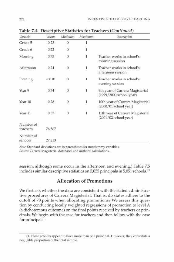
session, although some occur in the afternoon and evening.) Table 7.5includes similar descriptive statistics on 5,055 principals in 5,051 schools.91
Allocation of Promotions
We first ask whether the data are consistent with the stated administra-tive procedures of Carrera Magisterial. That is, do states adhere to thecutoff of 70 points when allocating promotions? We assess this ques-tion by conducting locally weighted regressions of promotion to level A(a dichotomous outcome) on the final points received by teachers or prin-cipals. We begin with the case for teachers and then follow with the casefor principals.
222 INCENTIVES TO IMPROVE TEACHING
Grade 5 0.23 0 1
Grade 6 0.22 0 1
Morning 0.75 0 1 Teacher works in school’s morning session
Afternoon 0.24 0 1 Teacher works in school’s afternoon session
Evening < 0.01 0 1 Teacher works in school’s evening session
Year 9 0.34 0 1 9th year of Carrera Magisterial (1999/2000 school year)
Year 10 0.28 0 1 10th year of Carrera Magisterial(2000/01 school year)
Year 11 0.37 0 1 11th year of Carrera Magisterial(2001/02 school year)
Number of teachers 76,567
Number of schools 27,213
Note: Standard deviations are in parentheses for nondummy variables.Source: Carrera Magisterial databases and authors’ calculations.
Table 7.4. Descriptive Statistics for Teachers (Continued)Variable Mean Minimum Maximum Description
91. Three schools appear to have more than one principal. However, they constitute anegligible proportion of the total sample.

223TEACHER AND PRINCIPAL INCENTIVES IN MEXICO
Table 7.5. Descriptive Statistics for PrincipalsVariable Mean Minimum Maximum Description
Education 8.40 0 15 Points awarded for educational (1.62) degrees
Experience 7.78 0 10 Points awarded for years of (2.25) experience
Peer review 9.09 0 10 Points awarded for peer review (1.44) by principals’ colleagues
Federal 0.89 0 11.11 Points awarded for participationtraining (2.53) in federal-level training courses
State 2.78 0 5 Points awarded for participation training (2.41) in state-level training courses
Principal test 17.33 5 28 Points awarded for principal (3.71) knowledge test
Initial points 46.27 9.8 74.31 Sum of the previous 7 variables(7.25)
Initial points < 50 0.74 0 1
Initial points 50–70 0.25 0 1
Initial points ≥ 70 <0.01 0 1
School 11.73 5.76 20 Points awarded for meanperformance (1.79) score of students and teachers
in school
Final points 58.00 16.8 85.91 Sum of initial points and school (7.79) performance
Final points ≥ 70 0.07 0 1
Promoted 0.04 0 1 Promoted to level A
Attempts 3.40 1 9 Number of attempts at (2.37) promotion to level A, including
current attempt
Male 0.65 0 1
Morning 0.77 0 1 School meets in the morning
Afternoon 0.23 0 1 School meets in the afternoon
(Continued)

Teachers
Figure 7.1 graphs the fitted values against final points for various sam-ples (sample sizes are available in table 7.4). Panel A includes the samplefrom 3 later years of the program. It suggests that the probability of beingpromoted to level A is essentially zero for teachers scoring below 70. Forteachers scoring above 70, the probability sharply rises to just below 0.8,and it appears quite steady regardless of the score. Similar results areobtained when dividing the sample by year (see panels B, C, and D).
Similar results were obtained by estimating a linear probability model,in which promotion was regressed on the final point score and its square,as well as on a dummy variable indicating whether the score is 70 orhigher. The coefficient on this last variable is reported in the first row oftable 7.6, and it suggests that the probability of promotion rises by 0.73for teachers above the cutoff. In other specifications, which are notreported here, we conditioned on other observable teacher variables,including gender, grade level, and session of instruction, but their coeffi-cients were not statistically significant.92
224 INCENTIVES TO IMPROVE TEACHING
Evening <0.01 0 1 School meets in the evening
Year 9 0.39 0 1 9th year of Carrera Magisterial(1999/2000 school year)
Year 10 0.26 0 1 10th year of Carrera Magisterial(2000/01 school year)
Year 11 0.35 0 1 11th year of Carrera Magisterial(2001/02 school year)
Number of principals 5,055
Number of schools 5,051
Note: Standard deviations are in parentheses for nondummy variables.Source: Carrera Magisterial databases and authors’ calculations.
Table 7.5. Descriptive Statistics for Principals (Continued)Variable Mean Minimum Maximum Description
92. Because the final allocation of promotions really occurs at the state level, the previ-ous results might occur if 32 states applied 32 different—but deterministic—cutoffs above 70(for example, Chiapas applying a cutoff of 74, above which 100 percent of teachers are pro-moted, and so on). Thus, we conducted the exercise in figure 7.1 again, dividing the sample byeach year and state. The results (which are not reported here) suggested that teachers in indi-vidual states almost always experience a sharp rise in the probability of promotion above 70,but that the probability is rarely 1 for such teachers.
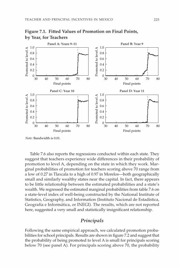
Table 7.6 also reports the regressions conducted within each state. Theysuggest that teachers experience wide differences in their probability ofpromotion to level A, depending on the state in which they work. Mar-ginal probabilities of promotion for teachers scoring above 70 range froma low of 0.27 in Tlaxcala to a high of 0.97 in Morelos—both geographicallysmall and similarly wealthy states near the capital. In fact, there appearsto be little relationship between the estimated probabilities and a state’swealth. We regressed the estimated marginal probabilities from table 7.6 ona state-level index of well-being constructed by the National Institute ofStatistics, Geography, and Information (Instituto Nacional de Estadística,Geografía e Informática, or INEGI). The results, which are not reportedhere, suggested a very small and statistically insignificant relationship.
Principals
Following the same empirical approach, we calculated promotion proba-bilities for school principals. Results are shown in figure 7.2 and suggest thatthe probability of being promoted to level A is small for principals scoringbelow 70 (see panel A). For principals scoring above 70, the probability
225TEACHER AND PRINCIPAL INCENTIVES IN MEXICO
0
0.2
0.4
0.6
0.8
1.0
Prom
oted
to le
vel A
30 40 50 60 70 80Final points
0
0.2
0.4
0.6
0.8
1.0
Prom
oted
to le
vel A
30 40 50 60 70 80Final points
0
0.2
0.4
0.6
0.8
1.0
Prom
oted
to le
vel A
30 40 50 60 70 80Final points
0
0.2
0.4
0.6
0.8
1.0Pr
omot
ed to
leve
l A
30 40 50 60 70 80Final points
Panel A: Years 9–11 Panel B: Year 9
Panel C: Year 10 Panel D: Year 11
Note: Bandwidth is 0.01.
Figure 7.1. Fitted Values of Promotion on Final Points, by Year, for Teachers

226 INCENTIVES TO IMPROVE TEACHING
Table 7.6. Determinants of Teacher Promotion, by StateCoefficient on Standard
Sample final points ≥ 70 error N R2
Full sample 0.73 (0.01) 76,567 0.69
State subsample (> 0.73) 0.83 (0.01) 37,283 0.80
State subsample (< 0.73) 0.63 (0.02) 39,284 0.59
Aguascalientes 0.92 (0.06) 657 0.88
Baja California 0.61 (0.05) 2,696 0.60
Baja California Sur 0.57 (0.11) 283 0.73
Campeche 0.95 (0.05) 698 0.95
Chiapas 0.80 (0.10) 2,008 0.70
Chihuahua 0.88 (0.03) 2,289 0.84
Coahuila 0.88 (0.05) 1,589 0.86
Colima 0.75 (0.10) 389 0.62
Distrito Federal 0.57 (0.04) 5,648 0.51
Durango 0.71 (0.08) 1,648 0.69
Guanajuato 0.74 (0.04) 5,200 0.74
Guerrero 0.71 (0.07) 4,500 0.71
Hidalgo 0.85 (0.06) 1,557 0.82
Jalisco 0.69 (0.04) 4,453 0.65
State of Mexico 0.80 (0.02) 11,529 0.78
Michoacán 0.82 (0.05) 2,696 0.82
Morelos 0.97 (0.03) 773 0.97
Nayarit 0.76 (0.10) 526 0.72
Nuevo León 0.87 (0.03) 2,787 0.84
Oaxaca 0.89 (0.06) 2,313 0.87
Puebla 0.66 (0.09) 4,343 0.63
Querétaro 0.70 (0.11) 653 0.75
Quintana Roo 0.48 (0.06) 835 0.46
San Luis Potosí 0.72 (0.08) 1,446 0.64
Sinaloa 0.58(Continued)

227TEACHER AND PRINCIPAL INCENTIVES IN MEXICO
(0.06) 2,557 0.59
Sonora 0.68 (0.07) 1,510 0.67
Tabasco 0.90 (0.07) 1,086 0.89
Tamaulipas 0.59 (0.05) 2,004 0.68
Tlaxcala 0.27 (0.10) 514 0.37
Veracruz 0.63 (0.05) 5,170 0.59
Yucatán 0.82 (0.06) 1,186 0.77
Zacatecas 0.62 (0.09) 1,024 0.60
Notes: Robust standard errors are corrected for school-level clustering. Each row reports a
Table 7.6. Determinants of Teacher Promotion, by State (Continued)Coefficient on Standard
Sample final points ≥ 70 error N R2
0
0.2
0.4
0.6
0.8
1.0
Prom
oted
to le
vel A
30 40 50 60 70 80Final points
0
0.2
0.4
0.6
0.8
1.0
Prom
oted
to le
vel A
30 40 50 60 70 80Final points
0
0.2
0.4
0.6
0.8
1.0
Prom
oted
to le
vel A
30 40 50 60 70 80Final points
0
0.2
0.4
0.6
0.8
1.0
Prom
oted
to le
vel A
30 40 50 60 70 80Final points
Panel A: Years 9–11 Panel B: Year 9
Panel C: Year 10 Panel D: Year 11
Note: Bandwidth is 0.05.
Figure 7.2. Fitted Values of Promotion on Final Points, by Year, for Principals

sharply rises to just below 0.6. Similar results are obtained when dividingthe sample by year (see panels B, C, and D). Table 7.7 suggests that theprobability of promotion rises by 0.44 for principals above the cutoff.
Table 7.7 also includes regression results divided by state. They sug-gest that principals experience wide differences in their probability ofpromotion to level A, depending on the state in which they work. Mar-ginal probabilities of promotion for principals scoring above 70 range froma low of zero in Campeche, Tlaxcala, and Zacatecas to a perfect probabilityin Nayarit. All of those states rank in the middle or lower end of the wealthdistribution. As with teachers, there is little relationship between the esti-mated probabilities and a state’s wealth. We again regressed the marginalprobabilities from table 7.7 on a state-level index of well-being. The results,which are not reported here, suggested a small and statistically insignifi-cant relationship.
Empirical Strategy
This section describes two empirical strategies that will be used to estimatewhether the incentives offered by Carrera Magisterial to teachers and prin-cipals were related to any changes in student or school performance. Tosimplify the exposition, we will fully describe the strategies for the teachercase only. However, in the last part of this section, we note differencesthat arise in the analysis of principals.
Incentives in Carrera Magisterial
The objective of this chapter is to assess whether Carrera Magisterialcaused increases in the mean of classroom achievement, perhaps byimproving teachers’ incentives to exert effort in the classroom. The datacontain observations only on teachers who have consented to be assessedin a given year. However, we argue next that subgroups of teachers—which are often quite large—experienced weaker incentives to improvetheir classroom’s mean achievement. Those teachers will serve as theneeded counterfactual.
As we previously described, 70 points are determined by the teacher’sbackground characteristics, such as formal education, experience, train-ing courses, and teacher’s test score. Another 10 points are determined bypeer review, but those ratings are generally high (the sample mean is 9.2).All of those factors are assessed in advance of collecting the students’ testscores. The scoring procedure is well publicized through materials dis-tributed to teachers and through national and state-level Web sites.93
228 INCENTIVES TO IMPROVE TEACHING
93. See http://www.sep.gob.mx/wb2/sep/sep_617_carrera_magisterial.

229TEACHER AND PRINCIPAL INCENTIVES IN MEXICO
Table 7.7. Determinants of Principal Promotion, by StateCoefficient on Standard
Sample final points ≥ 70 error N R2
Full sample 0.44 (0.01) 5,055 0.34
State subsample (> 0.44) 0.67 (0.02) 1,939 0.54
State subsample (< 0.44) 0.29 (0.02) 3,116 0.22
Aguascalientes 0.98 (0.20) 28 0.67
Baja California 0.41 (0.10) 133 0.29
Campeche 0.00 — 31 —
Chiapas 0.26 (0.05) 138 0.25
Chihuahua 0.45 (0.12) 98 0.31
Coahuila 0.69 (0.10) 125 0.44
Colima 0.51 (0.16) 45 0.35
Distrito Federal 0.41 (0.05) 452 0.34
Durango 0.25 (0.07) 114 0.18
Guanajuato 0.27 (0.07) 169 0.4
Guerrero 0.43 (0.04) 398 0.27
Hidalgo 0.79 (0.05) 135 0.83
Jalisco 0.15 (0.05) 228 0.09
State of Mexico 0.72 (0.03) 1,076 0.61
Michoacán 0.34 (0.05) 341 0.19
Morelos −0.23 (1.00) 10 0.14
Nayarit 1.00 — 23 —
Nuevo León 0.99 (0.11) 65 0.68
Oaxaca 0.37 (0.05) 244 0.36
Puebla 0.02 (0.11) 174 0.1
Querétaro 0.03 (0.12) 43 0.69
Quintana Roo 0.53 (0.11) 41 0.52
San Luis Potosí 0.37 (0.09) 83 0.25
Sinaloa 0.26 (0.07) 156 0.24
Sonora 0.29(Continued)
230 INCENTIVES TO IMPROVE TEACHING
(0.14) 35 0.16
Tabasco 0.77 (0.08) 94 0.75
Tamaulipas 0.54 (0.10) 158 0.46
Tlaxcala 0.00 — 33 —
Veracruz 0.17 (0.04) 297 0.14
Yucatán 0.6 (0.11) 51 0.53
Zacatecas 0.00 — 31 —
Notes: Robust standard errors are corrected for school-level clustering. Each row reports a
Table 7.7. Determinants of Principal Promotion, by State (Continued)
Coefficient on StandardSample final points ≥ 70 error N R2
94. Ortiz Jiménez (2003) refers to the issue disapprovingly in an official publication ofCarrera Magisterial that was distributed free of charge to all teachers.
Given the large number of teachers promoted, even within particularschools, it is likely that teachers share information about procedures andoutcomes. Finally, there is anecdotal evidence that teachers are aware oftheir position in the scoring process; therefore, many suffer from a maladyreferred to as “point-itis.”94
In this context, let us consider how the program might alter teachers’incentives to improve student achievement. The final assessment score(the final points received) can be expressed as f(X, A), where X is a vectorof the teacher’s background characteristics and A is the mean achievementof the teacher’s students. Likewise, A = a(X, Z, e), where Z is a vector ofstudents’ background characteristics (such as parental schooling) thatdetermine achievement and e is the chosen effort of each teacher. Addi-tional effort is presumed to be costly for teachers.
A substantial portion of teachers’ scores is determined before students’test scores are collected. These are the initial points received. Assume thatteachers possess sufficient knowledge to calculate the initial points as f(X, 0),or the score they would receive when A = 0. From this calculation, it isapparent that some teachers face weak incentives to improve their stu-dents’ achievement. If the initial points are greater or equal to 70, thenteachers already fall above the promotion cutoff and have no additionalincentive to exert costly effort over the course of the year. Similarly, if theinitial points are below 50, then teachers cannot be promoted, even if theyobtain the full 20 points awarded for students’ test scores. Again, theirincentives to exert additional effort to improve those test scores are weak.

Table 7.4 suggests that the first group is quite small. The mean of thedummy variable initial points greater than or equal to 70 is less than 0.01.The group was larger in earlier years of the program, when more experi-enced and highly educated teachers vied for promotion. In contrast, thesecond group constitutes the majority of the sample (the mean of thedummy variable of initial points below 50 is 0.85). The essential premise ofthis paper is to show that teachers were unlikely to exert effort towardthe pursuit of an unattainable reward.
When initial points are between 50 and 70, teachers may face strongerincentives to improve their students’ test scores. More specifically, theyare assumed to choose a level of effort, e*, so that their final points aref(X, a(X, Z, e*)) = 70. As teachers’ initial points cross the 50-point threshold,one would anticipate a tipping point in effort. Such teachers would movefrom minimum effort to maximum effort. This hypothesis forms the basisof the first empirical strategy, which is akin to a regression-discontinuitydesign.
Empirical Strategy 1
Panel A in figure 7.3 portrays a stylized version of this approach. In theabsence of Carrera Magisterial, there would likely be a positive relation-ship between the initial points—an index of teacher observables—andthe mean classroom test score of teachers. This relationship is portrayedwith a straight line in panel A, although the functional form is indeter-minate. One source of this relationship is the causal effect of teacherattributes on student outcomes. It is also rooted in correlations betweenobservable teacher attributes and unobserved teacher or student attrib-utes. For example, one might anticipate that better teachers—gauged bytheir degrees or experience—sort into the classrooms of higher-achievingstudents, as measured by socioeconomic status. Although this sortingwould alter the functional form of the relationship, one would still anticipatea smooth relationship.
As teachers cross the 50-point threshold, they face incentives to sub-stantially increase their achievement and, hence, their effort. This situationwould be evidenced by a break in the relationship between their initialpoints and test scores, which is illustrated by the dotted line segment. Asteachers’ initial points increase, however, the additional achievement andeffort required to reach the promotion cutoff becomes progressivelysmaller. Eventually, close to 70, the achievement and effort required toreach the promotion cutoff is minimal, and there will be little break, if any.
The magnitude of the break at 50 will likely vary across teachers, whosurely recognize that some classroom achievement will result from theirown background characteristics (the X’s) and the characteristics of theirstudents (the Z’s). Thus, some teachers whose initial points equal 50 will
231TEACHER AND PRINCIPAL INCENTIVES IN MEXICO

find that less effort is required to reach 70 (for example, those with highersocioeconomic status and higher-achieving students). Others will find thatsubstantial effort is required (such as those with lower socioeconomic sta-tus and lower-achieving students).
As an initial test, we will estimate
where the points from the classroom test score of the ith teacher are a func-tion of the initial points, a dummy variable indicating a value between 50and 70, and an error term. Further specifications will divide the 50–70 inter-val into a smaller series of dummy variables (in which the dummy vari-able indicating the leftmost interval should capture the break). We willalso add controls for a limited number of observed teacher variables, aswell as school fixed effects that control for unobserved school, teacher, andstudent variables that are constant within schools.
( . )7 1 500 1 2Testscorei i i= + + ≤( ) +β β β εInitialpoints Initialpoints < 70i
232 INCENTIVES TO IMPROVE TEACHING
Weakincentives
Strongerincentives
Weakincentives
All states
9
10
11
12
Tes
t sco
re
30 50 70 90Initial points
Weakincentives
Strongerincentives
Weakincentives
9
10
11
12
Tes
t sco
re
30 50 70 90Initial points
Panel A: Empirical strategy 1
States withweaker incentives
States withstronger incentives
Panel B: Empirical strategy 2
Figure 7.3. Stylized Portrayal of Empirical Strategy

As a sharper test of the presence of a break in classroom test scoresaround the discontinuity, we will further estimate
within subsamples of teachers whose values of the initial points fall withinsuccessively narrower bands around 50. Again, additional specificationswill control for observed teacher variables and school fixed effects.
A plausible explanation for a discontinuous relationship between theinitial points and the test scores—gauged by β2—would be a programeffect. Yet it is possible that a sharp break would not be observed, even inthe presence of an effect for many individual teachers. Suppose that someteachers whose initial points equal 50 will derive substantial disutilityfrom the effort required to obtain higher test scores; thus, the expectedaward would not outweigh the disutility. Such teachers would need toattain a higher value of initial points (thus exerting a smaller e*) beforethe disutility of effort was outweighed. In the extreme, some teachersmight find the required effort so onerous that they would exert no effortat any value of initial points between 50 and 70. If a teacher’s preferencesregarding effort are heterogeneous, then the dotted segment in panel Amay resemble a hump-like spline.
It would be difficult to convincingly attribute a smooth relationship(albeit a curiously nonlinear one) to the effects of Carrera Magisterial. Analternative explanation, for example, is that the nature of student andteacher sorting intensifies at higher values of initial points. Perhapshigher-achieving students in a school opt into the classrooms of betterteachers—in part, because the latter are observed to exert more effort.Anecdotally, at least, parents have little control over classroom assignmentin the Mexican public school system. However, it would still be desirableto corroborate any program effect (or lack thereof) with another empiricalstrategy.
Empirical Strategy 2
The evidence on the state-level allocation of promotions provides onealternative. Recall that teachers receiving a final score of 70 or above haddifferent probabilities of being promoted, depending on their state of res-idence. Thus, the expected value of the awards was different. We willassume that teachers in states with higher probabilities face relativelystronger incentives to exert effort than their counterparts in states withlower probabilities. Nonetheless, teachers in all states whose initial pointsare lower than 50 are assumed to face weak incentives.
The empirical strategy is illustrated in panel B of figure 7.3. It adds adashed line, representing states where teachers face lower probabilities of
( . )7 2 0 1 2Testscorei i i= + + ≥( ) +β β β εInitialpoints Initialpoints 50i
233TEACHER AND PRINCIPAL INCENTIVES IN MEXICO

promotion (and weaker incentives) below the solid line that now repre-sents states where teachers have higher probabilities of promotion (andstronger incentives). The former serves as a counterfactual for the latterin a difference-in-differences framework. If we observe a hump between50 and 70 in the strong-incentive group, the same relationship shouldbe attenuated in the counterfactual group. The empirical strategy restson the assumption that the functional form of relationship of the strong-incentive group would be the same as the weak-incentive group in theabsence of the incentive difference. We estimate the difference-in-differencesin a regression framework:
where Highprob is a dummy variable indicating that the ith teacher livesin a state with relatively higher promotion probabilities. The coefficient onthe interaction (β4) identifies the effect of the differential incentivesbetween the two groups. Other specifications are further conditioned onteacher observables and school fixed effects.
Differences in Empirical Strategy in the Principal Case
Similar to our case of teachers, we argue in the case of principals that sub-groups experienced weaker incentives to improve their classrooms’ meanachievement. Those principals will serve as the needed counterfactual.
Also similar to our case of teachers, if the principals’ initial points aregreater than or equal to 70, then the principals already fall above the pro-motion cutoff and have no additional incentive to exert costly effort overthe course of the year. If their initial points are below 50, principals can-not be promoted, even if they obtain the full 20 points awarded for schoolperformance. Again, their incentive to exert additional effort to improvethose scores is weak. Table 7.5 suggests that the group of principals fac-ing stronger incentives is quite small. The mean of the dummy variableof initial points ≥70 is again less than 0.01. The group of principals facingweaker incentives constitutes the majority of the sample (the mean of thedummy variable of initial points < 50 is 0.74).
As we described, 70 points are determined by the principal’s backgroundcharacteristics, such as formal education, experience, training courses, anda principal test score. Another 10 points are determined by supervisor eval-uations, but those ratings are generally high (the sample mean is 9.1). Allof those elements are assessed in advance of collecting the students’ testscores. Unlike the case for teachers, however, a portion of the principal’s 20-point school performance score is assessed at the same time that princi-pals are obtaining part of their initial points score. Specifically, half theschool performance points are awarded for teacher-specific test scores,
TestscoreHighprob
Highprob
i
i i
i i i
= ++ ≤ ≥( ) + ( )+ ≤ <( ) ∗ ( ) +
β ββ ββ ε
0 1
2 3
4
Initialpoints50 Initialpoints 7050 Initialpoints 70
i
234 INCENTIVES TO IMPROVE TEACHING

which are collected each year in March. Thus, the principals have a year-long incentive (or at least one lasting until March) to encourage teachers toprepare better for their own test scores. Thus, it will be difficult to determinewhether any effects for principals stem from efforts to improve students’achievement or from efforts to improve teachers’ test scores. Unfortunately,our school performance data are not broken down into the two 10-pointcomponents.
Results for Teachers
Empirical Strategy 1
Figure 7.4 reports preliminary evidence that can be used to visually iden-tify an effect. We performed locally weighted, smoothed regressions of testscores on initial points at various bandwidths. Panel A graphs the fittedvalues obtained from a bandwidth of 0.01, whereas panels B, C, and Duse successively wider ones. There is a positive and apparently linear rela-tionship between the index of teacher observables and test scores. How-ever, there is little evidence of a discontinuity in the relationship wheninitial points equal 50. A very small hump is observed between 50 and 55,
235TEACHER AND PRINCIPAL INCENTIVES IN MEXICO
Tes
t sco
re
Initial points Initial points
Tes
t sco
re
Tes
t sco
reT
est s
core
Initial points Initial points
Panel A: Bandwidth = 0.01 Panel B: Bandwidth = 0.03
Panel C: Bandwidth = 0.05 Panel D: Bandwidth = 0.1
10
10.5
11
11.5
12
30 40 50 60 70 8010
10.5
11
11.5
12
30 40 50 60 70 80
10
10.5
11
11.5
12
30 40 50 60 70 8010
10.5
11
11.5
12
30 40 50 60 70 80
Figure 7.4. Fitted Values of Classroom Test Scores on InitialPoints, by Bandwidth for Teachers

most notably in panels B and C. If one attributes this hump to a programeffect—and we do not hazard such an interpretation—it would be quitesmall. The “effect” appears roughly equal to 0.2 test score points for aclassroom in this narrow range of initial points, equivalent to less than 0.1standard deviations.
Table 7.8 reports regression evidence on these points. Column 1 regressestest scores on initial points and initial points between 50 and 70. All othercontrols are omitted, providing the best analogue to the previous visualevidence. The statistically significant coefficient on initial points (0.04)implies that a one standard deviation increase will lead to a 0.12 stan-dard deviation in classroom test scores. The dummy variable is positive,though small and statistically insignificant. It represents an averageacross all individuals in this interval. Column 2 adds more controls forteacher observables as well as state-level dummies, but the results arequite similar. Column 3 further controls for school-level dummies, relyingon within-school variation that appears to be substantial. The coeffi-cient on initial points falls by more than half, although it is still signifi-cant. This result suggests that school-level fixed effects are absorbingsome variation in teacher or student unobservables that are correlatedwith teacher observables.
Columns 4 through 6 control for initial points between 50 and 55, inan effort to better capture any perturbation in the functional form. Thecoefficients on the dummy variables are small though statistically signifi-cant in the first two specifications, roughly consistent with figure 7.4.However, the effect disappears upon controlling for school fixed effects.One might be concerned that this result occurs simply because little vari-ation exists within schools, but this absence does not appear to be the case.Overall, 46,209 teacher observations are made in a school where all teach-ers have initial points below 50 and 2,248 are made in a school where allteachers have initial points greater than or equal to 50. The remaining28,110 observations are from schools with teachers on either side of 50.
Columns 7 through 9 report less restrictive specifications, splitting the50–70 interval into four dummy variables. There is an even smaller, mar-ginally significant coefficient on initial points between 50 and 55 that againdisappears on the inclusion of school dummies. The other coefficients arenot statistically significant (although the thinness of the sample, especiallywhen initial points are greater than 65, does not suggest that we wouldbe able to precisely estimate these coefficients).95
Table 7.9 reports estimates of equation 7.2 that focus more intently on thevicinity of the hypothesized discontinuity. The samples are limited toteachers whose initial points are close to 50—within 10, 5, and 3 points,respectively. Panel A reports coefficients on a dummy variable that is equalto 1 when initial points are above 50 (all regressions also control for a con-
236 INCENTIVES TO IMPROVE TEACHING
95. Only 204 observations have values of initial points above 65.

237T
EA
CH
ER
AN
DP
RIN
CIPA
LIN
CE
NT
IVE
SIN
ME
XIC
O
Table 7.8. Teachers’ Initial Points and Classroom Test ScoresDependent variable: test score
(1) (2) (3) (4) (5) (6) (7) (8) (9)
Initial points 0.043** 0.037*** 0.016*** 0.042** 0.036*** 0.017*** 0.044** 0.038*** 0.015***(0.002) (0.002) (0.003) (0.002) (0.001) (0.002) (0.002) (0.002) (0.003)
Initial points 50–70 0.026 0.020 0.013 — — — — — —(0.042) (0.039) (0.054)
Initial points 50–55 — — — 0.129** 0.083** −0.012 0.090* 0.060 0.008(0.042) (0.040) (0.054) (0.045) (0.043) (0.058)
Initial points 55–60 — — — — — — −0.104 −0.063 −0.002(0.062) (0.058) (0.079)
Initial points 60–65 — — — — — — −0.158 −0.085 0.224(0.107) (0.101) (0.139)
Initial points 65–70 — — — — — — −0.284 −0.189 0.264(0.231) (0.225) (0.357)
R2 0.02 0.13 0.56 0.02 0.13 0.56 0.02 0.13 0.56
Controls? No Yes Yes No Yes Yes No Yes Yes
State fixed effects? No Yes No No Yes No No Yes No
School fixed effects? No No Yes No No Yes No No Yes
Note: The total number of regressions is 76,567. *** indicates statistical significance at 1 percent, ** at 5 percent, and * at 10 percent. Robust standard errorsare in parentheses, adjusted for school-level clustering. Controls include Male, Afternoon, Evening, Year 10, Year 11, Grade 4, Grade 5, and Grade 6.

238IN
CE
NT
IVE
ST
OIM
PR
OV
ET
EA
CH
ING
Table 7.9. Teachers’ Initial Points and Classroom Test Scores, within Narrow BandsDependent variable: test score
±10 points from cutoff ±5 points ±3 points
(1) (2) (3) (4) (5) (6) (7) (8) (9)
Panel AInitial points ≥ 50 0.015 −0.051 −0.129 −0.021 −0.028 −0.122 −0.086 −0.095 −0.179
(0.062) (0.058) (0.097) (0.089) (0.084) (0.216) (0.117) (0.111) (0.434)[43,491] [43,491] [43,491] [18,134] [18,134] [18,134] [10,162] [10,162] [10,162]
Panel BInitial points ≥ 51.2 0.006 −0.031 −0.115 0.086 0.063 −0.039 −0.048 −0.066 −0.154
(0.065) (0.061) (0.107) (0.093) (0.089) (0.242) (0.120) (0.114) (0.427)[38,273] [38,273] [38,273] [15,720] [15,720] [15,720] [8,994] [8,994] [8,994]
Panel CInitial points ≥ 54.1 −0.180* −0.086 −0.027 −0.176 −0.087 −0.003 −0.166 −0.085 −0.124
(0.076) (0.072) (0.146) (0.110) (0.104) (0.307) (0.141) (0.133) (0.570)[25,830] [25,830] [25,830] [11,283] [11,283] [11,283] [6,852] [6,852] [6,852]
Panel DInitial points ≥ 55.4 −0.227** −0.158** 0.041 −0.277* −0.296*** −0.227 −0.045 −0.119 −0.589
(0.084) (0.079) (0.173) (0.119) (0.113) (0.363) (0.154) (0.147) (0.642)[21,513] [21,513] [21,513] [9,683] [9,683] [9,683] [5,822] [5,822] [5,822]
Controls? No Yes Yes No Yes Yes No Yes Yes
State fixed effects? No Yes No No Yes No No Yes No
School fixed effects? No No Yes No No Yes No No Yes
Notes: *** indicates statistical significance at 1 percent, ** at 5 percent, and * at 10 percent. Robust standard errors are in parentheses, adjusted forschool-level clustering. The N of each regression is in brackets. All regressions control for a continuous measure of initial points. Additional controlsinclude Male, Afternoon, Evening, Year 10, Year 11, Grade 4, Grade 5, and Grade 6.
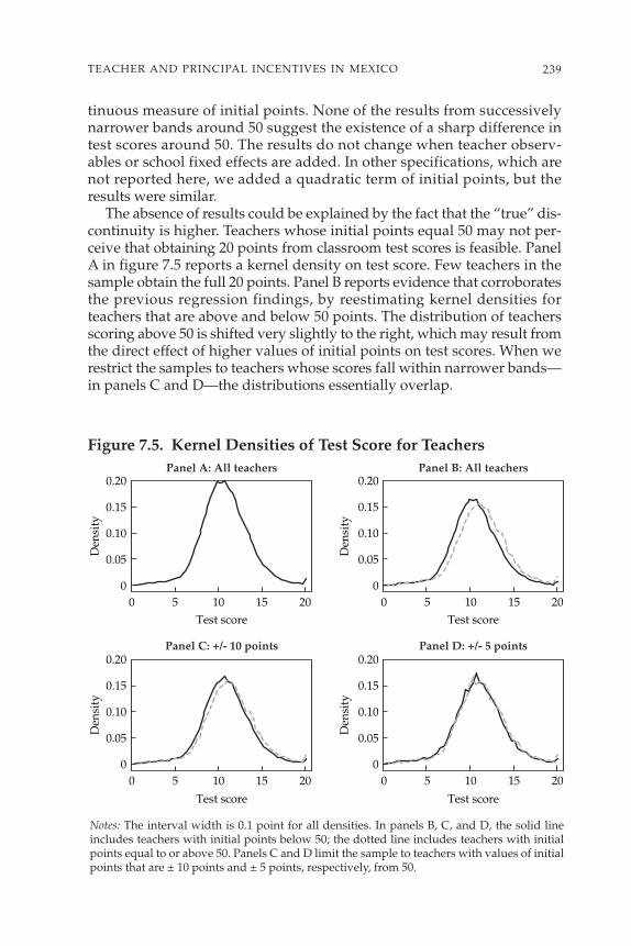
tinuous measure of initial points. None of the results from successivelynarrower bands around 50 suggest the existence of a sharp difference intest scores around 50. The results do not change when teacher observ-ables or school fixed effects are added. In other specifications, which arenot reported here, we added a quadratic term of initial points, but theresults were similar.
The absence of results could be explained by the fact that the “true” dis-continuity is higher. Teachers whose initial points equal 50 may not per-ceive that obtaining 20 points from classroom test scores is feasible. PanelA in figure 7.5 reports a kernel density on test score. Few teachers in thesample obtain the full 20 points. Panel B reports evidence that corroboratesthe previous regression findings, by reestimating kernel densities forteachers that are above and below 50 points. The distribution of teachersscoring above 50 is shifted very slightly to the right, which may result fromthe direct effect of higher values of initial points on test scores. When werestrict the samples to teachers whose scores fall within narrower bands—in panels C and D—the distributions essentially overlap.
239TEACHER AND PRINCIPAL INCENTIVES IN MEXICO
Den
sity
Test score Test score
Den
sity
Den
sity
Den
sity
Test score Test score
Panel A: All teachers Panel B: All teachers
Panel C: +/- 10 points Panel D: +/- 5 points
00 5 10 15 20
0.05
0.10
0.15
0.20
00 5 10 15 20
0.05
0.10
0.15
0.20
00 5 10 15 20
0.05
0.10
0.15
0.20
00 5 10 15 20
0.05
0.10
0.15
0.20
Notes: The interval width is 0.1 point for all densities. In panels B, C, and D, the solid line includes teachers with initial points below 50; the dotted line includes teachers with initial points equal to or above 50. Panels C and D limit the sample to teachers with values of initial points that are ± 10 points and ± 5 points, respectively, from 50.
Figure 7.5. Kernel Densities of Test Score for Teachers

Teachers might implicitly consider a higher discontinuity. To explorethis possibility, we note that the 99th, 95th, and 90th percentiles in the testscore sample are 18.8, 15.9, and 14.6, respectively. The three values implydiscontinuities of 51.2, 54.1, and 55.4, respectively. Panels B, C, and D intable 7.9 report additional regression results using these discontinuities,but none of the coefficients are positive and significant. The same resultshold when we control for a quadratic term of initial points.
One might also posit that teachers, in assessing the “maximum” value ofclassroom test scores that is feasible, rely on their knowledge of the statedistribution in test scores, rather than on their knowledge of the nationalone. Thus, we repeated the previous exercise by estimating the 99th per-centile of test scores within each of Mexico’s states. Then, we constructeda dummy variable equal to 1 if a teacher’s value of initial points fell abovethe discontinuity implied by the state-specific test score. This variable wasused in the same regressions reported in table 7.9. The same exercise wasrepeated for the 95th and 90th percentiles. None of the results suggestedthat teachers scoring above discontinuities, however defined, would obtainhigher classroom test scores.
Empirical Strategy 2
The first strategy did not turn up positive and robust effects. However, thelack of a sharp break could result from heterogeneous teacher preferences. Toexamine this possibility, we identified two groups of teachers: (a) thoseworking in states where scoring above 70 increases the probability of pro-motion by 0.73 or more (the estimated probability in the full sample) and(b) those working in states with probabilities of less than 0.73. The probabil-ities for each group, estimated separately, are 0.83 and 0.63, respectively(see table 7.6). The difference of 0.2 implies that the expected value of scoringabove 70 is 32 percent higher for teachers in the first group. Hence, we dubthe two groups the “stronger-incentive” and “weaker-incentive” groups.
We repeat the previous section’s visual exercise by obtaining separate fit-ted values for each group (see figure 7.6). The solid and dashed lines in eachpanel indicate the strong- and weak-incentive groups, respectively. Wheninitial points are below 50, we surmise that both groups face weak incen-tives and should have similar functional forms. That similarity seems tobe the case in all panels, and it is also the case in a formal test.96 Above 50,one might anticipate a divergence in the lines in the presence of a program
240 INCENTIVES TO IMPROVE TEACHING
96. We limited the samples to observations with initial points below 50. We then regressedthe test score variable on (a) the initial points variable, (b) a continuous variable containingthe state-specific probability, and (c) the interaction between the two variables (with robuststandard errors adjusted for school-level clustering). We could not reject the null that thecoefficient on the interaction is zero.
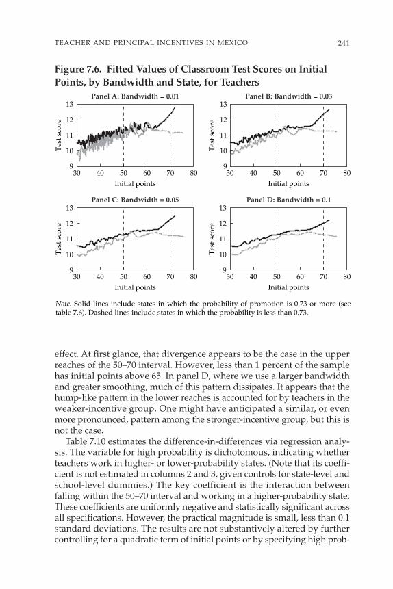
effect. At first glance, that divergence appears to be the case in the upperreaches of the 50–70 interval. However, less than 1 percent of the samplehas initial points above 65. In panel D, where we use a larger bandwidthand greater smoothing, much of this pattern dissipates. It appears that thehump-like pattern in the lower reaches is accounted for by teachers in theweaker-incentive group. One might have anticipated a similar, or evenmore pronounced, pattern among the stronger-incentive group, but this isnot the case.
Table 7.10 estimates the difference-in-differences via regression analy-sis. The variable for high probability is dichotomous, indicating whetherteachers work in higher- or lower-probability states. (Note that its coeffi-cient is not estimated in columns 2 and 3, given controls for state-level andschool-level dummies.) The key coefficient is the interaction betweenfalling within the 50–70 interval and working in a higher-probability state.These coefficients are uniformly negative and statistically significant acrossall specifications. However, the practical magnitude is small, less than 0.1standard deviations. The results are not substantively altered by furthercontrolling for a quadratic term of initial points or by specifying high prob-
241TEACHER AND PRINCIPAL INCENTIVES IN MEXICO
9
10
11
12
13
9
10
11
12
13
9
10
11
12
13
9
10
11
12
13
Tes
t sco
re
30 40 50 60 70 80Initial points
Tes
t sco
re
30 40 50 60 70 80Initial points
Tes
t sco
re
30 40 50 60 70 80Initial points
Tes
t sco
re
30 40 50 60 70 80Initial points
Panel A: Bandwidth = 0.01 Panel B: Bandwidth = 0.03
Panel C: Bandwidth = 0.05 Panel D: Bandwidth = 0.1
Note: Solid lines include states in which the probability of promotion is 0.73 or more (see table 7.6). Dashed lines include states in which the probability is less than 0.73.
Figure 7.6. Fitted Values of Classroom Test Scores on InitialPoints, by Bandwidth and State, for Teachers

242 INCENTIVES TO IMPROVE TEACHING
Table 7.10. Teachers’ Initial Scores and Classroom Test Scores:Difference-in-Differences
Dependent variable: test score
(1) (2) (3)
Initial points 0.042*** 0.037*** 0.016***(0.002) (0.002) (0.003)
Initial points 50–70 0.141*** 0.094* 0.118*(0.052) (0.049) (0.067)
Higher probability 0.404*** — —(0.029)
(Initial points 50–70) × (Higher probability) −0.213*** −0.142** −0.204**(0.063) (0.059) (0.082)
Controls? No Yes Yes
State fixed effects? No Yes No
School fixed effects? No No Yes
Notes: The N of all regressions is 76,567. Robust standard errors are in parentheses, adjustedfor school-level clustering; *** indicates statistical significance at 1 percent, ** at 5 percent,and * at 10 percent. Additional controls include Male, Afternoon, Evening, Year 10, Year 11,Grade 4, Grade 5, and Grade 6.
ability as a continuous variable—measuring state-specific probabilities—rather than a dichotomous variable.
One might further posit that, in some states, the probabilities are morestable across time, perhaps suggesting that such teachers are more respon-sive to such information in determining their level of effort. We identifieda subset of 15 states in which three estimated probabilities—estimated sep-arately across each year of data—were never more than 0.2 apart. Theregression results were similar.
Robustness Checks
Thus far, the results do not indicate that teachers with stronger incentivesproduce higher achievement than teachers with weaker incentives. Thissection probes this conclusion further by carrying out a number of robust-ness checks.
First, it is possible that effects are heterogeneous across groups of teachers.We reestimated the regressions from the discontinuity specification incolumns 4–6 of table 7.9 and from the difference-in-differences specifica-tion in columns 1–3 in table 7.10. The regressions were estimated withinsubsamples defined by year of the sample (9, 10, and 11); by the teacher’sgender; by the teacher’s educational level; and by the socioeconomic index
of the community where the school is located.97 None of the coefficientswere positive, and they were statistically significant at 5 percent.
Second, it is possible for teachers to reenter the assessment process insubsequent years, even if they are denied promotion in the current year.About one-third of our sample is attempting promotion for the first time,while the rest are appearing for the second time or more. The latter groupis older and, hence, more likely to fall within the 50–70 interval. That factmay lead to higher or lower achievement among their students, perhapsbecause of experience or demoralization. Thus, we reestimated the samespecifications as in the previous paragraph, while including a series ofdummy variables that control for promotion attempts (ranging from thesecond to the tenth attempt, relative to the first). In other regressions, welimited the sample to first-timers. None of those results altered the previousconclusions.
Third, one might question whether all components of the initial pointsthat a teacher receives are exogenous. The most likely candidate is the teach-ers’ test that is administered in March, which contributes 28 points to thescore. Suppose that teachers can allocate their effort across two activities:(a) classroom teaching and (b) “cramming” for the teachers’ test, which isbased on subject matter. If cramming is a successful strategy, then onemight expect that teachers who retake the test—as described in the lastparagraph—would experience test score gains.98 To test this hypothesis,we regressed the teacher test data on a series of dummy variables that con-trol for promotion attempts (again, ranging from the second to the tenthattempt), in addition to dummy variables indicating the assessment yearand teacher fixed effects. None of the coefficients on the promotion attemptdummy variables were statistically significant. This result provides somelimited evidence that—at least among a subsample of teachers who tookthe test multiple times—that teachers’ test scores are relatively stable.
Nonetheless, imagine that additional effort might influence one’s owntest score. In such a case, the relevant initial points measure, from theteacher’s perspective, would include all the previous components exceptfor the teachers’ test. The outcome variable would now be the sum of thestudents’ test score and the individual teacher’s test score (ranging from0 to 48). The relevant discontinuity, in this case, is 22. Teachers scoringbelow 22 face weak incentives, because they cannot score above 70, even
243TEACHER AND PRINCIPAL INCENTIVES IN MEXICO
97. We defined three levels of education: (a) no higher-education degree, (b) a teacher’scollege degree or equivalent, and (c) a university degree or higher. The socioeconomic indexis by INEGI. It is at the community level and is based on a range of variables, including illit-eracy, utility access of homes, and income. We divided the sample into three groups, whichare based on terciles of the index.
98. In a similar vein, Vigdor and Clotfelter (2003) demonstrate gains on SAT scoresamong students who take the test multiple times, perhaps because of learning or greaterfamiliarity with the test format.

with the full 48 points on the tests for teachers and students. If their scoresare above 22, teachers allocate their efforts across teaching effort and cram-ming effort. To assess that possibility, we reestimated all regressions withthe revised dependent and independent variables, but there was still noevidence of a positive effect.
Discussion
In a program as large and costly as Carrera Magisterial, it is important toask why there is no apparent effect. There are several possible explanations.First, teachers may perceive that the mean test score of their class is a noisymeasure. Analyses of test score data in the United States and Chile sug-gest that the error variance of school-level mean test scores is substantiallylarger when the school enrollment is smaller, because of sampling variation(Chay, McEwan, and Urquiola 2003; Kane and Staiger 2001). In the presentcase, individual classroom means are assessed. The smaller samples implyrelatively noisier measures. The original Carrera Magisterial data do notcontain either class sizes or school enrollments, but we obtained thepupil–teacher ratio of each school in grades 3–6 (the grades correspond-ing to our sample) in program year 10. We then graphed the test score ofeach classroom against its school’s pupil–teacher ratio (see figure 7.7). Apattern emerges, as in prior research, in which mean performance is morevariable in smaller classrooms (as proxied by the pupil–teacher ratio). Ofcourse, the vast majority of observations are drawn from schools withpupil–teacher ratios of less than 50.
Suppose teachers perceive that the mean test score in a given year isindeed a noisy measure that fluctuates widely from year to year. Becauseteachers are allowed to participate in the assessment more than once—andpoints received from other factors appear stable—teachers may simplydecide that it is better to reduce costly effort and to wait for a year in whichtheir class receives a transitorily high mean score.
Second, it is possible that the disutility of additional effort always out-weighs the expected utility of receiving an award. Nevertheless, the extra-ordinarily generous awards—more than 20 percent of subsequent careerwages—render this argument somewhat less plausible.
Third, it is possible that teachers do not have a clear understanding ofthe classroom production technology. They may be willing to increaseeffort but are unsure of how to fruitfully expend effort toward improv-ing their students’ test scores. This scenario might be likely if the teach-ers are not aware of the content of the student test. However, the testsare grade specific and are designed to reflect the content of the existingcurriculum and textbooks (Ortiz Jiménez 2003). Another possibility is thatthere is not enough time—in the 2 to 3 months between the teacher test(when teachers more or less can calculate their “exogenous” score) and the
244 INCENTIVES TO IMPROVE TEACHING

student test—for them to be able to substantially improve their students’performance, even with high levels of effort.
Results for Principals
Empirical Strategy 1
Figure 7.8 reports evidence that can be used to visually identify an effect.Panel A graphs the fitted values obtained from a bandwidth of 0.01,whereas panels B, C, and D use successively wider ones. There is a positiveand apparently linear relationship between the index of observables forprincipals and school performance scores. However, there is little evidenceof a discontinuity in the relationship when initial points equal 50. A smallhump is observed just before 60, roughly equal to 0.4 test score points fora classroom in this narrow range of initial points, which is equivalent toless than a quarter of a standard deviation.
Table 7.11 reports regression evidence on these points. Column 1regresses test scores on initial points and on initial points between 50 and 70.All other controls are omitted, providing the best analogue to the previousvisual evidence. The statistically significant and positive coefficient on ini-
245TEACHER AND PRINCIPAL INCENTIVES IN MEXICO
0
5
10
15
20
Tes
t sco
re
0 50 100 150Pupil–teacher ratio in grades 3–6
Figure 7.7. Test Scores and Pupil–Teacher Ratios in Year 10 for Teachers
Note: The horizontal line is located at the sample mean (10.8).

tial points (0.044) implies that an increase of one standard deviation in ini-tial points (7.25 units) is associated with an increase of close to one-fifthof a standard deviation in the school performance variable. The dummyvariable for the 50–70 interval is positive, though small and statisticallyinsignificant. Column 2 adds more controls for observables of principals, aswell as for state-level dummies, but the results are quite similar. Column 3further controls for school fixed effects, which are, in fact, individual fixedeffects. The coefficient on initial points becomes insignificant as fixed effectsabsorb most of the variation between principals and, as expected, explaina large proportion (0.82) of the variation in school performance scores.Columns 4–6 report less restrictive specifications, splitting the 50–70 intervalinto four dummy variables. There is a larger, albeit negative, coefficient oninitial points between 60 and 65.
Empirical Strategy 2
We next identified two groups of principals: (a) those working in stateswhere scoring above 70 increases the probability of promotion by 0.44 ormore (the estimated probability in the full sample), and (b) those workingin states with probabilities of less than 0.44. The probabilities for eachgroup, estimated separately, are 0.67 and 0.29, respectively (see table 7.7).
246 INCENTIVES TO IMPROVE TEACHINGT
est s
core
Initial points Initial points
Tes
t sco
re
Tes
t sco
reT
est s
core
Initial points Initial points
Panel A: Bandwidth = 0.01 Panel B: Bandwidth = 0.03
Panel C: Bandwidth = 0.05 Panel D: Bandwidth = 0.1
10.0
10.5
11.0
11.5
12.0
30 40 50 60 70 8010.0
10.5
11.0
11.5
12.0
30 40 50 60 70 80
10.0
10.5
11.0
11.5
12.0
30 40 50 60 70 8010.0
10.5
11.0
11.5
12.0
30 40 50 60 70 80
Figure 7.8. Fitted Values of Classroom Test Scores on InitialPoints, by Bandwidth for Principals

The difference of 0.38 implies that the expected value of scoring above70 is more than 130 percent higher for principals in the first group. Hence,we dub the two groups the “stronger-incentive” and “weaker-incentive”groups.
We repeat the previous section’s visual exercise, obtaining separatefitted values for each group (see figure 7.9). The solid and dashed lines ineach panel indicate the strong-incentive and weak-incentive groups,respectively. When initial points are below 50, we surmise that bothgroups face weak incentives and should have similar functional forms.That similarity seems to be the case in all panels, and it is also the case ina formal test.99 When the initial points are above 50, one might anticipate
247TEACHER AND PRINCIPAL INCENTIVES IN MEXICO
Table 7.11. Principals’ Initial Points and School Performance Scores
Dependent variable: school performance
(1) (2) (3) (4) (5) (6)
Initial points 0.044** 0.037*** 0.011 0.050** 0.043*** 0.012(0.005) (0.005) (0.009) (0.006) (0.005) (0.01)
Initial points 50–70 0.06 0.074 −0.092 — — —(0.083) (0.081) (0.119)
Initial points 50–55 — — — 0.059 0.07 −0.085(0.086) (0.084) (0.121)
Initial points 55–60 — — — 0.062 0.077 −0.124(0.128) (0.125) (0.191)
Initial points 60–65 — — — −0.370* −0.363** −0.333(0.174) (0.17) (0.297)
Initial points 65–70 — — — −0.472 −0.507* 0.176(0.272) (0.266) (0.494)
R2 0.04 0.10 0.82 0.04 0.10 0.82
Controls? No Yes Yes No Yes Yes
State fixed effects? No Yes No No Yes No
School fixed effects? No No Yes No No Yes
Notes: The N of all regressions is 5,055. *** indicates statistical significance at 1 percent, ** at5 percent, and * at 10 percent. Standard errors are in parentheses. Controls include Male,Afternoon, Evening, Year 10, and Year 11.
99. We limited the samples to observations with initial points below 50. We thenregressed the test score variable on (a) the initial points variable, (b) a continuous variablecontaining the state-specific probability, and (c) the interaction between the two variables(with robust standard errors adjusted for school-level clustering). We could not reject the nullthat the coefficient on the interaction is zero.

a divergence in the lines in the presence of a program effect. At first glance,that divergence appears to be the case close to 50 (where most of the sam-ple is concentrated). In panel D, which uses a larger bandwidth andgreater smoothing, much of this pattern dissipates.
Table 7.12 estimates the difference-in-differences via regression analysis.The variable for high probability is dichotomous, indicating whether prin-cipals work in higher- or lower-probability states. (Note that its coefficientis not estimated in columns 2 and 3, given controls for state-level andschool-level dummies.) The key coefficient is the interaction betweenfalling within the 50–70 interval and working in a higher-probability state.The coefficients are positive, but they are small in magnitude and statisti-cally insignificant across all specifications.
Overall, the results do not suggest that principals improved school per-formance in their promotion years. In addition, there is limited evidence tosuggest that after reaching an initial point score of 60, principals tend to beassociated with lower school performance. Those results include animportant caveat, however. A more thorough analysis of those and otherpossibilities would necessitate more data to be able to separate the schoolperformance score into its two components: the students’ scores and the
248 INCENTIVES TO IMPROVE TEACHING
9
10
11
12
14
13
9
10
11
12
13
9
10
11
12
13
9
10
11
12
13
Tes
t sco
re
30 40 50 60 70 80Initial points
Tes
t sco
re
30 40 50 60 70 80Initial points
Tes
t sco
re
30 40 50 60 70 80Initial points
Tes
t sco
re
30 40 50 60 70 80Initial points
Panel A: Bandwidth = 0.01 Panel B: Bandwidth = 0.03
Panel C: Bandwidth = 0.05 Panel D: Bandwidth = 0.1
Note: Solid lines include states in which the probability of promotion is greater than 0.44 (see table 7.7). Dashed lines include states in which the probability is less than 0.44.
Figure 7.9. Fitted Values of Classroom Test Scores on Initial Points, by Bandwidth and State

teachers’ scores. It might be that principals have somewhat more control(or power to affect) teachers’ scores than students’ scores. For example,principals could give teachers time to prepare for the Carrera Magisterialtests or could provide guidance and training. The possibility must also beconsidered that principals exert control over which teachers participatein any given year. In so doing, they may be able to select higher-scoringteachers or teachers with the highest-scoring students. This chapter hasnot investigated that possibility.
Conclusions
This chapter has provided empirical evidence on the student and schoolperformance effects of Mexico’s Carrera Magisterial program for teachersand principals. In estimating the effects, we relied on the fact that some par-ticipating teachers and principals face weaker incentives, because they faceinsurmountable barriers to promotion in a given year or simply because theylive in a state where high-scoring participants face a lower probability of pro-motion. For both teachers and principals, the chapter did not find robustevidence that Mexican teachers facing stronger incentives actually improvedstudent achievement in the year in which they were assessed.
These results have several potential implications. First, an essentialpremise of this chapter is that many Mexican teachers and principals—
249TEACHER AND PRINCIPAL INCENTIVES IN MEXICO
Table 7.12. Principals’ Initial Scores and Classroom Test Scores:Difference-in-Differences
Dependent variable: school performance
(1) (2) (3)
Initial points 0.043*** 0.037*** 0.01(0.005) (0.005) (0.009)
Initial points 50–70 0.061 0.024 −0.217(0.095) (0.094) (0.146)
Higher probability (dichotomous) 0.224*** — —(0.059)
(Initial points 50–70) × (Higher probability) 0.038 0.122 0.265(0.117) (0.116) (0.193)
Controls? No Yes Yes
State fixed effects? No Yes No
School fixed effects? No No Yes
Notes: The N of all regressions is 5,055. Standard errors in parentheses; *** indicates statisti-cal significance at 1 percent. Additional controls include Male, Afternoon, Evening, Year 10,and Year 11.
85 percent and 74 percent of our sample respectively—faced weaker incen-tives, even when participating in the Carrera Magisterial assessment. Evendisregarding the subsequent empirical findings, this conclusion is sober-ing. It suggests that a revised assessment process could restrict eligibilityto groups of participants that are most likely to face strong incentives (thusincurring savings from a reduced assessment burden). Similarly, onemight place increasing weight on students’ test scores in the promotionformula (for both teachers and principals), thus expanding the “treated”range of initial points beyond the 50–70 interval.
Second, one could imagine a scenario under which student test scoresdid improve in the case of teachers or where evidence of improvementsin school performance was much stronger. Even under this optimisticscenario, the cost of a one-shot gain in students’ test scores or school per-formance is clearly high. After receiving their promotions, particularly atthe highest level, teachers and principals once again face weak incentivesto improve the achievement of later student cohorts.100 Yet they continueto receive substantial monetary rewards throughout their careers. It isunclear, for example, why Mexico should not simply invest in a relativelycheap tutoring program and obtain a 0.2 standard deviation gain, as wasdone in Chile (Chay, McEwan, and Urquiola 2003).
Third, it would be appropriate to base a permanent and costly promotionon more than a single classroom’s test scores or on the average scores of par-ticipating Carrera Magisterial teachers in the school, which in some yearscan mean only one or two teachers. On the one hand, combining variousyears’ test scores might diminish the noise of a mean test score measurethat is based on a small sample of students or teachers. On the other hand,it would provide added incentives for participants to exert effort in morethan the particular year in which they are being considered for promotion.
Fourth, it is possible that large and permanent wage increases have suc-ceeded in attracting a more qualified pool of teacher applicants (and per-haps teacher hires) in the past decade, in part because they link teacherwages to teacher test scores.101 That research question was not addressed inthis chapter. Even if this possibility were the case, however, it might havebeen accomplished at a lower administrative cost by simply implement-ing across-the-board wage increases or by modifying the wage scheduleto place greater weight on teacher competencies.
250 INCENTIVES TO IMPROVE TEACHING
100. Teachers may, however, decide to participate each year so they can obtain a highscore that they can use later for promotion. However, once a teacher or principal obtains asufficiently high score in any given year, the incentive to keep participating in the program(and thus to improve in the school or classroom) diminishes.
101. Teachers’ test scores generally have more demonstrable links to student achievementin Mexico and elsewhere (see, for example, Hanushek 2002; Santibáñez 2003). We are inter-ested here only in the effects on the teacher applicant pool, because all public school princi-pals in Mexico must be first hired as teachers.

References
Bossert, S. T., D. C. Dwyer, B. Rowan, and G. V. Lee. 1982. “The Instruc-tional Management Role of the Principal.” Educational AdministrationQuarterly 18(3): 34–64.
Chay, K. Y., P. J. McEwan, and M. Urquiola. 2003. “The Central Role ofNoise in Evaluating Interventions That Use Test Scores to RankSchools.” NBER Working Paper 10118. National Bureau of EconomicResearch, Cambridge, Mass.
Courty, P., and G. Marschke. 2004. “An Empirical Investigation of Gam-ing Responses to Explicit Performance Incentives.” Journal of LaborEconomics 22: 23–56.
Cullen, J. B., and R. Reback. 2002. “Tinkering toward Accolades: SchoolGaming under a Performance Accountability System.” University ofMichigan, Ann Arbor. Processed.
Eberts, R. W., and J. A. Stone. 1988. “Student Achievement in PublicSchools: Do Principals Make a Difference?” Economics of EducationReview 7(3): 291–99.
Education Week. 2004. Quality Counts 2004. Bethesda: Editorial Projects inEducation.
Figlio, D. N. 2002. “Can Public Schools Buy Better Teachers?” Industrialand Labor Relations Review 55: 686–99.
Figlio, D. N., and L. S. Getzler. 2002. “Accountability, Ability, and Dis-ability: Gaming the System.” Working Paper 9307. National Bureauof Economic Research, Cambridge, Mass.
Figlio, D. N., and J. Winicki. Forthcoming. “Food for Thought: The Effectsof School Accountability Plans on School Nutrition.” Journal of PublicEconomics 89(2): 381–94.
Gates, S. M., J. S. Ringel, L. Santibáñez, K. E. Ross, and C. H. Chung. 2003.Who Is Leading Our Schools? An Overview of School Administrators andTheir Careers. Santa Monica, Calif.: Rand.
251

Glewwe, P., N. Ilias, and M. Kremer. 2003. “Teacher Incentives.” WorkingPaper 9671. National Bureau of Economic Research, Cambridge, Mass.
Hallinger, P., and J. Murphy. 1986. “Instructional Leadership in EffectiveSchools.” Elementary School Journal 86: 217–47.
Hanushek, E. A. 2002. “Publicly Provided Education.” In A. J. Auerbach andM. Feldstein, eds., Handbook of Public Economics (vol. 4). Amsterdam:North-Holland.
Hanushek, E. A., and M. E. Raymond. 2002. “Improving EducationalQuality: How Best to Evaluate Our Schools?” In Y. K. Kodrzycki, ed.,Education in the 21st Century: Meeting the Challenges of a Changing World.Boston: Federal Reserve Bank of Boston.
Jacob, B. A., and S. D. Levitt. 2003. “Rotten Apples: An Investigation ofthe Prevalence and Predictors of Teacher Cheating.” Quarterly Journalof Economics 118: 843–78.
Kane, T. J., and D. O. Staiger. 2001. “Improving School Accountability Mea-sures.” Working Paper 8156. National Bureau of Economic Research,Cambridge, Mass.
Lavy, V. 2002. “Evaluating the Effect of Teachers’ Group PerformanceIncentives on Pupil Achievement.” Journal of Political Economy 110(6):1286–317.
Murnane, R. J., and D. K. Cohen. 1986. “Merit Pay and the EvaluationProblem: Why Most Merit Pay Plans Fail and a Few Survive.” HarvardEducational Review 56: 1–17.
Ortiz Jiménez, M. B. 2003. Carrera Magisterial: Un proyecto de desarrollo pro-fesional. Cuadernos de Discusión 12. Secretaría de Educación Pública,Mexico City.
Prendergast, C. 1999. “The Provision of Incentives in Firms.” Journal ofEconomic Literature 37 (March): 7–63.
Presidency of the Mexican Republic. 1992. Decreto para la celebración de con-venios en el marco del acuerdo nacional para la modernización de la educaciónbásica (ANMEB). Diario Oficial de la Federación, May 19.
Santibáñez, L. 2003. “Why We Should Care if Teachers Get A’s: TeacherCharacteristics and Student Achievement in Mexico.” RAND, SantaMonica. Processed.
252 INCENTIVES TO IMPROVE TEACHING
SEP (Secretaría de Educación Pública). No date. Cronograma de actividadespara la operación de Carrera Magisterial, décimatercera etapa (ciclo escolar2003–2004). Mexico City.
———. 2003. Informe de labores 2003. Anexo 3. Mexico City.
Vigdor, J. L., and C. T. Clotfelter. 2003. “Retaking the SAT.” Journal ofHuman Resources 38: 1–33.
Zigarelli, M. A. 1996. “An Empirical Test of Conclusions from EffectiveSchools Research.” Journal of Educational Research 90(2): 103–10.
253TEACHER AND PRINCIPAL INCENTIVES IN MEXICO

8Decentralization of Education,
Teacher Behavior, and OutcomesThe Case of El Salvador’s EDUCO Program
Yasuyuki Sawada
and Andrew RagatzUniversity of Tokyo
El Salvador’s model for decentralized schools, Educación con Partici-pación de la Comunidad (Education with Community Participation, orEDUCO), presents a unique opportunity to evaluate the effect of decen-tralization on education. This chapter builds on a study by Jimenez andSawada (1999) that measured the effects on student outcomes of decen-tralizing educational responsibility to communities and schools. It fur-ther explores the effect of decentralization, this time focusing on how itaffects administrative processes and teacher behavior, and on how thosechanges affect student achievement and the quality of education.
In our empirical implementations, we control for school, community,and school participant (teacher, director, student) characteristics. We alsocontrol for sample selection bias using two methods. First, we use propen-sity score matching in an attempt to eliminate selection bias. Then we usea standard sample selection model to determine whether the level of biasin our model resulting from unobserved variables is significant. Theresults indicate that, interestingly, most administrative processes in EDUCOhave not shifted to the local level, if we compare it to traditional schools, butthat certain key administrative activities such as hiring and firing decisionsdo, in fact, differ significantly between EDUCO and traditional schools.
The more striking finding is that school associations tend to feel theyhave greater influence in virtually every administrative activity. Ourresults also indicate that decentralization may have a positive influence onteacher behavior. Although certain concerns exist in ability to measure
255
We would like to thank all the participants of the World Bank workshop on April 22, 2004.The many insightful comments we received were helpful in bringing out key messages andgreatly improved the content of our paper.

the abstract concept of teacher behavior, there does seem to be a statisti-cally significant “EDUCO effect.” This effect, in turn, may have a positiveinfluence on student performance.
Teachers play a central role in education. From a financial standpoint,teachers account for a large share of the total educational budget. From aquality of education standpoint, a talented, motivated teacher can have apositive effect on students. Conversely, a teacher who does not put mucheffort into creating a positive learning environment or who is frequentlyabsent can have a detrimental effect on student outcomes. Many studieshave demonstrated that, controlling for differences in students’ socioeco-nomic background, teachers constitute the most important determinantof student achievement.102 Creating an environment and providing incen-tives that promote positive teacher behavior, then, can be a critical com-ponent of improving education.
Many developing countries have recently adopted various models ofdecentralized school management, where communities play a larger rolein running the school (Bardhan 2002; Conning and Kevane 2002; Rai 2002;Stiglitz 1999; World Bank 2003). Theory suggests that decentralizationcan ease the problem that results from imperfect information, enable thepoor to amplify their voice in policymaking and strengthen the incentivesfor providers to serve effectively (World Bank 2003).103 This model ofschooling could potentially have a significant influence on teacher behav-ior and motivation. El Salvador’s decentralized school management pro-gram, EDUCO, provides a unique opportunity to explore the issue ofteacher behavior in a decentralized schooling model. This chapter exam-ines the EDUCO program in an attempt to better understand how theschooling model has affected teacher motivation and behavior, as well ashow those behavioral changes have affected student achievement.
This chapter builds on the study by Jimenez and Sawada (1999) that mea-sured the effects on student outcomes of decentralizing educational respon-sibility to communities and schools. We compare administrative activitiesand teacher behavior in EDUCO schools to those in traditional schools. Wecontrol for school, community (socioeconomic), and participant (teacher,director, and student) characteristics. We also control for sample selectionbias, using both propensity score matching and an exogenously determinedformula for targeting EDUCO schools as an instrumental variable.
Interestingly, the results indicate that many administrative processesin EDUCO have not dramatically shifted to the local level when comparedwith traditional schools. Yet, selective administrative activities such as hir-
256 INCENTIVES TO IMPROVE TEACHING
102. For recent examples, see Ehrenberg and Brewer (1995); Monk (1994); and Rivkin,Hanushek, and Kain (forthcoming).
103. In practice, in many centrally run government programs, the employees mightbecome accountable not to local beneficiaries but to central authorities. Because compensa-tion of teachers and doctors usually is not linked to their performance, their work incentivesare likely to be weak. As a result, salaried teacher absenteeism and tardiness are prevalentin many developing countries, especially in rural areas (Lockheed and others 1991, p. 101).

ing and firing decisions do, in fact, differ significantly between the twosystems. But striking decentralization differences emerged when measuringperceived amount of influence. School associations in EDUCO tend to feelthey have greater influence in virtually every administrative activity, eventhough many of those processes may still be carried out primarily at thenational level.
The results also indicate (a) that decentralization may have had a positiveeffect on teacher behavior, with teachers tending to show more motivationin EDUCO schools, and (b) that this increased motivation may, in turn, havehad a positive effect on student performance, as measured by mathematicsand Spanish achievement test scores and by school attendance.
The chapter is organized as follows. In the next section, we describe thebackground of the EDUCO program and give a simple comparison ofEDUCO and traditional schools. Then we make an empirical study of theEDUCO program. The section shows empirical evidence on how decentral-ization has changed the process for teacher management, how decentraliza-tion changes have affected teacher behavior, and to what extent changes inteacher behavior have affected the educational outcome. Finally, we concludewith a brief discussion of the policy implications of our empirical findings.
The Case of El Salvador’s EDUCO Program
Background
The EDUCO program is based on an inventive decentralized schoolingmodel that evolved during El Salvador’s civil war. In the 1980s, many ruralcommunities were cut off from, or had only limited access to, the traditionaleducation system. In many areas, the communities themselves took respon-sibility for providing educational opportunities for their children. By thelate 1980s, the national government saw the community model that hademerged as having great potential for efficiently and effectively providingeducation, particularly to isolated rural communities. With the support ofinternational agencies, the national government implemented the EDUCOprogram in 1990. The program is for both pre-primary and primary educa-tion and aims at decentralizing education by strengthening direct involve-ment and participation of parents and community groups (Jimenez andSawada 1999, 2001; Reimers 1997; World Bank 2003).
The EDUCO program was designed to achieve several goals. A primarygoal was to provide access to schools in the country’s poorest and most-isolated rural communities. Other goals included supporting and encour-aging community participation in education, improving the quality ofpre-primary and primary schooling, and improving school-level manage-ment and administration by allowing the communities—who best knowtheir own schooling needs—to create and manage school priorities.
In EDUCO schools, the Community Education Association (AsociaciónComunal para la Educación, or ACE) plays a central role in school admin-
257DECENTRALIZATION OF EDUCATION

istration and management. The selection process of ACE members isdemocratic: ACE members are selected by votes of parents of all studentsat a biannual general assembly. ACEs are contracted by the Ministry ofEducation (MINED) to deliver a given curriculum to an agreed numberof students. ACEs are then responsible for contracting and removingteachers by closely monitoring teachers’ performance and for equippingand maintaining the schools. In short, the ACE members have power todecide the allocation of school resources and employment of teachers (fig-ure 8.1). The partnership between MINED and ACEs is expected toimprove school administration and management by reflecting localdemand needs more appropriately than that of traditional public schools.Conversely, a parents’ association (sociedad de padres de familia, or SdPF) incentrally managed traditional public schools has little or no administrativecapability over school personnel or budget.104
The initial indications are that the EDUCO program has accomplishedits primary goal of rapidly expanding access to education in remote ruralareas by using the demonstrated community interest as a platform (WorldBank 1997). One concern is whether this rapid expansion using a decentral-ized model has come at the expense of quality of education as the systemmoves away from traditional programs that provide education centrally.The theory favoring the decentralized model is that education quality willimprove because communities can better identify needs of the school andcan quickly respond. This increased sense of ownership could also fosterpride and greater dedication to ensuring that the school operates properly.
Similar to other decentralization studies in Latin America, a 1997 studyof the EDUCO program found that student achievement was positivelyaffected by decentralization (World Bank 1997). Jimenez and Sawada(1999) concluded that student achievement has not been adverselyaffected by the rapid deployment of EDUCO schools.
An area that is still not well understood for this type of decentralizationmodel is how it influences teacher behavior. This chapter focuses specifi-cally on differences in administrative processes and teacher behavior, aswell as on how teacher behavior affects student outcomes.
Data
The data were collected in October 1996 by MINED of El Salvador withthe assistance of the World Bank and the U.S. Agency for International
258 INCENTIVES TO IMPROVE TEACHING
104. In 1996, School Management Councils (Consejos Directivos Escolares, or CDEs) wereintroduced to the traditional schools in order to increase participation and democracy inschool management. The council is composed of a school director, teachers, parents of stu-dents, and students. Since 1998, CDEs have become legally mandatory for all traditionalschools. In the future, MINED intends to introduce community management into all tradi-tional schools through CDEs.

259DECENTRALIZATION OF EDUCATION
School Inputs — Management — TEACHER
ACE
Parents
Output
MINED
Input Decision
EmploymentDecision
Parent-TeacherMeetings
Home Teaching
Schooling
Strong InfluenceWeak Influence
EDUCO Schools
School Inputs — Management — TEACHER
SdPF
Parents
Output
MINED
Input Decision
EmploymentDecision
Parent-TeacherMeetings
Home Teaching
Schooling
Strong InfluenceWeak Influence
Traditional Schools
Source: Author’s illustration.
Figure 8.1. Comparison of EDUCO and Traditional Governance Structures
Development. The data set includes 311 primary schools, with data of1,555 students, and 596 ACE committee members, which were randomlysampled from the 3,634 primary schools (Jimenez and Sawada 1999).105
The surveys focused on third-grade sections for each school.
105. The survey was conducted again in 1998, with slightly different questionnaires anddifferent respondents. In the 1998 survey, the students in the 1996 survey were interviewedas well. See Jimenez and Sawada (2001).
The survey covered 162 of El Salvador’s 262 municipalities. Thosemunicipalities share responsibility with the central government for thedelivery of social services. The original sample was selected to capturedata for four types of schools—EDUCO, traditional, “mixed” (havingsome school sections under the EDUCO system and other sections underthe traditional system), and private. In this study, we dropped samplesfor private schools and traditional public schools located in urban areasbecause those samples are not comparable with rural EDUCO schools. Tohave the clearest distinction possible between EDUCO and traditional sys-tems, we also dropped the mixed schools. We were left with 37 pureEDUCO schools and 96 pure traditional rural schools.
The survey is composed of five questionnaires: student, parents, schooldirector, teacher, and parents’ association. In addition, we use variousmunicipality-level socioeconomic indicators, such as municipality-levelpoverty indices, infant mortality rates, and illiteracy rates.
Variables and Descriptive Statistics
Following are simple statistics that present a general picture of the differ-ences between EDUCO and traditional schools.
The selection criteria used for placing EDUCO schools target primarilythe poorest, most isolated rural communities. Acomparison of municipality’ssocioeconomic characteristics in table 8.1 reflects these criteria. In everycategory, community characteristics for the EDUCO schools show higherpoverty and lower education characteristics, with the exception of overagestudents in grades 7–9. This difference is most likely because in most of thepoorest communities schooling is not even offered for grades 7–9, so moststudents in those communities do not continue their education.
The descriptive statistics in table 8.2 show household socioeconomiccharacteristics to be much better for traditional school students than forEDUCO students. The parents of traditional school students have moreeducation than those of EDUCO students, with 54 percent of mothers orfemale guardians of traditional students having basic education, com-pared with 50 percent for EDUCO students. The same is true of the fathers’education. The educational differences are reflected also in the asset indi-cators. Fewer EDUCO parents have access to home ownership, electricity,sanitary services, and running water. These data all suggest that EDUCOstudents come from poorer backgrounds than traditional school students.Therefore, the EDUCO program has been successful in targeting poorersegments of the population.
Basic school characteristics found in table 8.3 are consistent with thepattern for the socioeconomic characteristics of students and households.Although the availability of sanitation is similar in both types of schools,fewer EDUCO schools have access to electricity or piped water.
260 INCENTIVES TO IMPROVE TEACHING

Data on teachers’ characteristics indicate that EDUCO teachers aremore likely to have finished a university education but are less experi-enced because EDUCO teachers typically are relatively young recent grad-uates. Although EDUCO teachers earn less without controlling for anydifferences in age, experience, or educational level, they tend to receivemore benefits than traditional school teachers.
As for classroom characteristics, there are no differences in accessibilityto textbooks in the two types of schools, but an EDUCO classroom typicallyhas fewer pupils and a larger number of books in the classroom library thana traditional school classroom has. Moreover, a multigrade setting is foundmore frequently in EDUCO schools than in traditional schools.
Regarding community participation issues, parents of EDUCO studentsparticipate more in school affairs. ACE members in EDUCO schools visitclassrooms about four times more often than their traditional counterparts.
261DECENTRALIZATION OF EDUCATION
Table 8.1. Means and Standard Deviations of Municipality-Level Socioeconomic VariablesVariable definitions EDUCO schools Traditional schools All schools
Poverty decile (1–10, with 1 3.59 4.82 4.48being poorest decile) (1.77) (2.00) (2.01)
Mortality rate (%) 38.44 34.68 35.72(17.45) (14.57) (15.45)
Illiteracy rate (%) 35.49 29.66 31.28(11.41) (10.75) (11.21)
Improvisational housing (%) 46.01 39.6 41.38(9.52) (11.72) (11.48)
Education rate, grades 1–6 (%) 38.42 46.04 43.92(10.92) (13.93) (13.56)
Education rate, grades 7–9 (%) 17.35 20.41 19.56(9.08) (10.78) (10.39)
Overage students, grades 1–6 (%) 53.00 50.37 51.10(5.62) (8.72) (8.05)
Overage students, grades 7–9 (%) 49.45 51.20 50.71(8.45) (12.61) (11.6)
Rural population (%) 71.96 67.74 68.94(21.3) (19.82) (20.26)
Number of observations 37 96 133
Note: Standard deviations in parentheses.Source: Author calculations using data from the 1996 MINED survey.
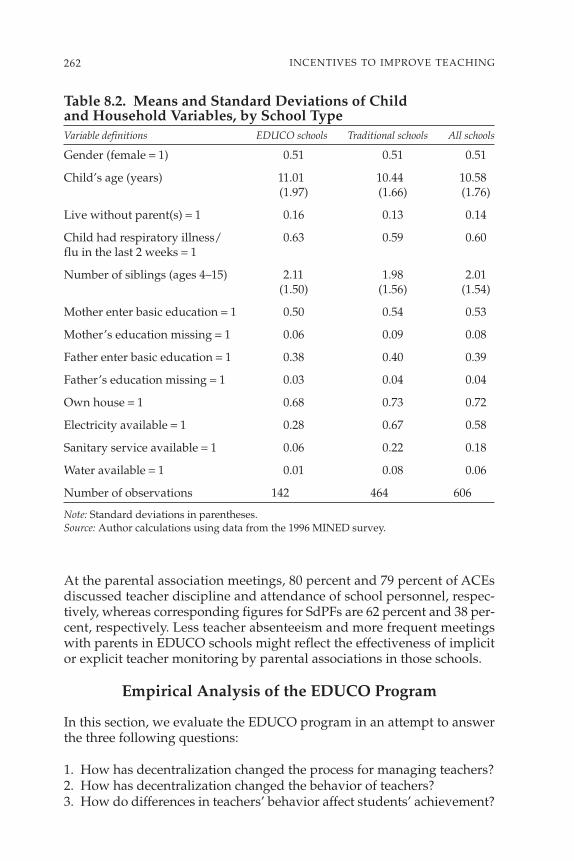
At the parental association meetings, 80 percent and 79 percent of ACEsdiscussed teacher discipline and attendance of school personnel, respec-tively, whereas corresponding figures for SdPFs are 62 percent and 38 per-cent, respectively. Less teacher absenteeism and more frequent meetingswith parents in EDUCO schools might reflect the effectiveness of implicitor explicit teacher monitoring by parental associations in those schools.
Empirical Analysis of the EDUCO Program
In this section, we evaluate the EDUCO program in an attempt to answerthe three following questions:
1. How has decentralization changed the process for managing teachers?2. How has decentralization changed the behavior of teachers?3. How do differences in teachers’ behavior affect students’ achievement?
262 INCENTIVES TO IMPROVE TEACHING
Table 8.2. Means and Standard Deviations of Child and Household Variables, by School TypeVariable definitions EDUCO schools Traditional schools All schools
Gender (female = 1) 0.51 0.51 0.51
Child’s age (years) 11.01 10.44 10.58(1.97) (1.66) (1.76)
Live without parent(s) = 1 0.16 0.13 0.14
Child had respiratory illness/ 0.63 0.59 0.60flu in the last 2 weeks = 1
Number of siblings (ages 4–15) 2.11 1.98 2.01(1.50) (1.56) (1.54)
Mother enter basic education = 1 0.50 0.54 0.53
Mother’s education missing = 1 0.06 0.09 0.08
Father enter basic education = 1 0.38 0.40 0.39
Father’s education missing = 1 0.03 0.04 0.04
Own house = 1 0.68 0.73 0.72
Electricity available = 1 0.28 0.67 0.58
Sanitary service available = 1 0.06 0.22 0.18
Water available = 1 0.01 0.08 0.06
Number of observations 142 464 606
Note: Standard deviations in parentheses.Source: Author calculations using data from the 1996 MINED survey.

Table 8.3. Means and Standard Deviations of School, Teacher,Classroom, and Community Variables, by School TypeVariable definitions EDUCO schools Traditional schools All schools
School variables:
Teacher–pupil ratio (school level) 0.05 0.03 0.04(0.09) (0.041) (0.056)
If sanitation or latrine is available 0.89 0.94 0.93 at school = 1
If electricity is available at 0.30 0.80 0.68school = 1
If piped water is available 0.12 0.38 0.32 at school = 1
Teacher and classroom variables:
If teacher finished a university 0.75 0.37 0.46 education = 1
Years of teaching experience 4.37 8.89 7.83(2.71) (6.87) (6.44)
Monthly base salary of 2,919.23 3,070.71 3,035.21 teacher (colon) (269.40) (574.84) (523.38)
If teacher receives bonus = 1 0.74 0.61 0.64
If all students have math 0.58 0.62 0.61 textbook = 1
If math textbook information 0.25 0.07 0.11 is missing = 1
If all students have language 0.59 0.59 0.59textbook = 1
If language textbook information 0.28 0.07 0.12 is missing = 1
If teacher teaches in multigrade 0.39 0.20 0.24classroom = 1
If multigrade information is 0.04 0.00 0.01missing = 1
Number of books in classroom 114.63 61.98 74.32 library (272.84) (166.42) (197.59)
If classroom library information 0.24 0.54 0.47 is missing = 1
Community participation variable:
Number of ACE or SpDF visits 5.65 1.56 2.52to classroom (6.59) (3.63) (4.82)
Number of observations 31 102 133
Note: Standard deviations in parentheses.Source: Author calculations using data from the 1996 MINED survey.

Each question is a logical progression that builds on the results of the pre-vious one. If one first better understands how EDUCO administrativeprocesses differ from those of traditional schools, then teacher behaviordifferences can be analyzed with a clearer lens, especially when evaluatingthe effects on student achievement.
In each section, we first form hypotheses, driving the structure of themodel used. Those hypotheses are discussed in more detail within eachsection, but here we provide a brief summary. First, EDUCO has thecharter of decentralizing administrative processes. Our hypothesis inanalyzing administrative processes, then, is that they would be moredecentralized in EDUCO schools and that participants at the local levelwould feel they have more influence. Second, for teacher behavior, ourhypothesis is based on the principal–agent model. In a more decentralizedschool, the teacher (agent) is being closely monitored by the school associa-tion (principal) rather than by a centralized body, as is the case in tradi-tional schools with the Ministry of Education. The hypothesis is that thisclose monitoring in EDUCO schools would lead to more-motivated teacherbehavior. Finally, regarding student achievement, our hypothesis is thatmore motivated teachers will have a positive effect on student achievement.
How Has Decentralization Changed the Process of Teacher Management?
To evaluate the effect of EDUCO program on teacher behavior, one mustfirst understand how administrative processes differ between EDUCOand traditional schools. The surveys of director, teacher, and schoolassociation members contain questions covering 29 administrative pro-cesses. For each process, the interviewees were asked whether theybelieve the major influence level of the process is at the national, depart-mental, or school level and how much influence they believe they havein the process, allowing for a comparison of perspectives by the differ-ent key participants (table 8.4). The former question gives an imperfectbut supportive measure of decentralization, while the latter questiongives a subjective assessment of one’s own influence in administrativeprocesses.
Our hypothesis is that administrative processes in EDUCO schools aremore decentralized than in traditional schools and that participants inEDUCO schools, particularly school association members, feel they havemore influence. Although this shift in influence is expected to be primarilyfrom the central to the local level, we also hypothesize that gains in influenceby one group within the schools (particularly school associations) could takeaway influence from other school members (particularly directors).
The survey questions give nice insights into perspectives of differentschool members and can create a clearer picture of how the EDUCO and
264 INCENTIVES TO IMPROVE TEACHING

traditional systems operate differently, but some issues should first benoted. First, the responses are subjective. The fact that we have responsesfrom three different perspectives allows a more objective picture to emerge,but subjective responses are generally not as reliable as hard data. Second,the question of major influence does not give an accurate measure of levelof decentralization. For example, a process that takes place at the nationallevel, such as determining teacher salary, may be answered as “national”by both traditional and EDUCO respondents. It may be, however, thatthe schools in one system do, in fact, have much more influence in theprocess, even though the final decision is made at the national level. Thisdifference would not be captured in the decentralization-level question butmight be reflected more in the amount of influence question. Finally,although the surveys are comprehensive and allow us to control for manyvariables, it is still likely that bias exists from unobserved characteristics.The issue of sample selection and unobserved bias, as well as how weaddress it, is discussed in detail in subsequent sections.
The Model of Administrative Process MeasurementThe models of EDUCO and traditional schools are structured so that theadministrative processes between the two systems may function differentlyand that the roles of different participants—directors, teachers, and schoolassociations—may also differ. To compare differences between EDUCO andtraditional schools, we first start with the following simple model:
where Yij is the decentralization measure by school i in an administrativeprocess j; D is an indicator variable of school type, where D equals 1 foran EDUCO school and D equals 0 for a traditional school; Z denotes avector of observed physical school-level characteristics; X represents a vec-
( . ) ,8 1 Y D Z X uij i i z i X i= + + +δ β β
265DECENTRALIZATION OF EDUCATION
Table 8.4. The Format of Questions on the Administrative ProcessQ1. The major influence of the process j is at what level?
1. National2. Departmental3. School
Q2. How much influence do you (as director, teacher, or association member) have inthe process j?
1. None2. A little3. Some4. A lot
Source: 1996 MINED Survey.

tor of characteristics of employees within the school; and C is a vector ofmunicipality m’s specific variables. In equation 8.1, the estimated coeffi-cient δ captures the “EDUCO effect” after controlling for observed differ-ences between EDUCO and traditional schools in school-level, employee,and community characteristics. The coefficient can be interpreted as theunobserved effect in EDUCO schools generated by the difference in schoolgovernance, organization, and resulting incentive mechanism, which areidentified by Hanushek (1995) and Kremer (1995) as important factors inproducing education.
This simple ordinary least squares (OLS) model may suffer from sampleselection and unobserved variable bias. To address that issue, we used twotechniques: propensity score matching and endogenous sample selection.
Propensity Score Matching106
In equation 8.2, denote that Y1 and Y0 represent outcome with and withouttreatment, respectively. Because an individual cannot be in both states,we cannot observe both Y1 and Y0. Instead, what we observe is
To measure the effect of treatment, the literature focused on the followingtwo quantities: average treatment effect (ATE) and average treatmenteffect on the treated (ATT). The ATE and ATT, respectively, are
There are several approaches to quantify the treatment effects. In thischapter, we use the propensity score matching method for the ATT and thesample selection method for the ATE.107
In the propensity score matching method, the comparison group ismatched to the treatment group on the basis of propensity score, wherepropensity score is defined as the conditional probability of receiving a treat-ment given pretreatment characteristics (Woodridge 2002). The propensityscore is estimated by using the probit model. Then we use a matchingmethod called weighted nearest-neighbor matching. Under this method,each treated unit is matched with the control unit with the closest propen-sity score.108
( . ) , , ,8 4 11 0E Y Y D Z X Ci i m− =( )
( . ) , ,8 3 1 0E Y Y Z X Ci i m−( )
( . )8 2 11 0Y D Y D Y≈ + −( )
266 INCENTIVES TO IMPROVE TEACHING
106. This section is based on Becker and Ichino (2002) and Woodridge (2002).107. Other methods include randomized experiments that became extremely popular in
development economics (Angrist and others 2002; Kremer 2003; Miguel and Kremer 2004;Schultz 2004).
108. We also use kernel matching, under which all treated units are matched with aweighted average of all control units with weights that are inversely proportional to the dis-tance between the propensity scores of treated units and controls. The results are not pre-sented in this chapter but are available upon request from the authors.

Endogenous Sample SelectionPlacement of EDUCO schools is not randomly determined. Program par-ticipation is affected by the targeting procedure in EDUCO schools. Fromthe beginning of the program in 1991–1992 to the time of the survey, theestablished policy is that the EDUCO schools function exclusively in themost distant, inaccessible rural areas. The government established a pri-ority list of municipalities that were to receive an EDUCO program accord-ing to poverty and education deficiency characteristics. To open a newEDUCO school, the community needed to have a student population atthe preschool and first-grade level, and the location of the new schoolcould not have another school within at least 4 kilometers. Finally andmore important, the community had to show interest in participating inthe administration of the school.
This endogenous placement procedure might generate an endogeneitybias if we estimate the model of equation 8.2 by using only OLS. For exam-ple, it is likely that a community highly motivated in educating its childrenreceived an EDUCO school. In that case, the error term of equation 8.2 and anunobserved factor affecting placements are likely to be positively correlated.
Hence, we also model explicitly the endogenous placement of EDUCOschools as follows:
where D* is a latent variable of the propensity of EDUCO placement. Theeconometric model of equations 8.2, 8.5, and 8.6 is called “treatment effectsmodel” in the literature (Greene 2003, pp. 787–89).109
Suppose that the error terms in equations 8.2 and 8.5 follow a jointNormal distribution with var(u) = σ2, var(v) = 1, and cov(u, v) = λ. Letthe functions, φ(•) and Φ(•) represent density and cumulative densityfunctions, respectively, of standard Normal distribution. Then there areseveral ways to estimate the model of equations 8.2, 8.5, and 8.6. We applyJames Heckman’s two-step estimation method to estimate the followingaugmented regression model:110
( . )*
*8 6
1 0
0 0D
if D
if Di
i
i
=>
>
( . ) *8 5 D W vi i i= +γ
267DECENTRALIZATION OF EDUCATION
109. A generalized version of the model is also called self-selection model (Lee 1978),switching regression model (Maddala 1983, pp. 117–22), Type 5 Tobit model (Amemiya 1985),and the model with dummy endogenous regressor (Angrist 1999).
110. We adjusted and estimated the consistent variance–covariance matrix because OLSestimation of the second step in the two-step procedure does not provide the consistentvariance–covariance matrix. We can also use the nonlinear least squares method to estimateequation 8.7.

When we estimate equation 8.7, we use estimated γ by the first-step pro-bit model of equations 8.5 and 8.6.
In equation 8.2, the critical focus is on the coefficient δ on the EDUCOdummy variable, D, where—controlling for community, school, andemployee characteristics—the effect of the EDUCO model on the givenadministrative process Y can be measured relative to the traditional schoolmodel. A crucial point to keep in mind is that the D gives an account ofhow EDUCO schools compare for the given administrative process rela-tive to traditional schools but does not show to what extent the processhas been decentralized in absolute terms.
Variables Used in AnalysisWe use the first question in table 8.4 to quantify the degree of decentral-ization for each school. The questions on major influence were answeredseparately by the three participants (directors, teachers, and associationmembers). We combine those responses by school to make an integratedindicator of decentralization for each school.111 The coefficient on theEDUCO dummy variable is interpreted to be the degree of decentralizationin EDUCO schools compared with traditional schools.
We use the second question in table 8.4 to quantify how much influ-ence the group or individual has on the process. The range of options isfrom 1 (no influence) to 4 (a lot of influence).112 In the regressions, a pos-itive coefficient in the EDUCO dummy variable indicates that in EDUCOschools the amount of influence is greater than in traditional schools,whereas a negative coefficient indicates that the influence is greater in tra-ditional schools.
Table 8.5 shows mean and standard deviation for both level of decen-tralization and perception of influence. The numbers allow for comparisonbetween EDUCO and traditional schools, as well as show magnitudes ofthe responses. For example, determine salary is extremely low for bothEDUCO and traditional schools, indicating that the activity occurs pri-marily at the national or departmental level in almost all cases, whereasspend school money occurs primarily at the school level in almost all casesfor both school systems.
( . )ˆˆ
ˆˆ
˜8 7 11
Y D Z X C DWW
DW
Wuz x m c= + + + + ( )
( ) + −( ) ( )− ( ) +δ β β β λ φ γ
γλ φ γ
γΦ Φ
268 INCENTIVES TO IMPROVE TEACHING
111. We constructed two indicators of the degree of decentralization. First, the administra-tive process takes place at the school level or not at the school level, so that if a response ofnational or department is given, then it receives a value of 0, whereas a response of school levelreceives a value of 1. We take the average of this binary indicator over three participants.
112. The survey originally used 1 = a lot of influence to 4 = no influence, but we flipped theresponses so that a higher number would represent more influence.

269D
EC
EN
TR
AL
IZA
TIO
NO
FE
DU
CA
TIO
N
Table 8.5. Means and Standard Deviations of Decentralization and Perceived Influence VariablesDecentralization Amount of perceived own influence
Weighted average Association Director Teacher
EDUCO Traditional Total EDUCO Traditional Total EDUCO Traditional Total EDUCO Traditional Total
Determine salary 0.14 0.06 0.08 3.00 2.89 2.96 1.05 1.36 1.27 1.28 1.17 1.20(0.24) (0.15) (0.18) (0.84) (0.78) (0.80) (0.23) (0.94) (0.82) (0.81) (0.62) (0.68)
Determine teacher incentives 0.42 0.34 0.36 2.44 1.83 1.99 2.26 2.17 2.20 2.00 1.40 1.55(0.35) (0.31) (0.32) (1.08) (1.03) (1.07) (1.26) (1.32) (1.30) (1.31) (0.84) (1.00)
Evaluate teacher 0.44 0.53 0.51 2.61 1.65 1.91 3.08 3.35 3.27 1.84 1.66 1.70(0.33) (0.31) (0.32) (1.11) (0.86) (1.02) (1.09) (1.00) (1.03) (1.13) (1.05) (1.07)
Give teacher incentives 0.35 0.37 0.36 2.41 1.91 2.05 2.13 2.28 2.24 1.85 1.39 1.50(0.33) (0.32) (0.32) (1.00) (1.05) (1.06) (1.31) (1.32) (1.32) (1.22) (0.79) (0.93)
Hire and fire administration 0.47 0.24 0.30 2.35 1.45 1.71 1.63 1.57 1.59 1.21 1.30 1.27(0.32) (0.31) (0.33) (1.17) (0.86) (1.04) (0.97) (0.99) (0.98) (0.57) (0.85) (0.78)
Hire and fire director 0.45 0.14 0.22 2.76 1.52 1.87 1.18 1.30 1.27 1.06 1.21 1.17(0.37) (0.24) (0.31) (1.02) (0.89) (1.08) (0.64) (0.81) (0.77) (0.25) (0.69) (0.61)
(Continued)

Table 8.5. Means and Standard Deviations of Decentralization and Perceived Influence Variables (Continued)Decentralization Amount of perceived own influence
Weighted average Association Director Teacher
EDUCO Traditional Total EDUCO Traditional Total EDUCO Traditional Total EDUCO Traditional Total
Hire and fire teacher 0.51 0.07 0.20 2.79 1.52 1.88 1.30 1.40 1.37 1.19 1.18 1.18(0.36) (0.17) (0.31) (1.13) (0.91) (1.13) (0.74) (0.84) (0.81) (0.54) (0.63) (0.60)
Spend school money 0.94 0.99 0.97 3.47 3.18 3.26 3.28 3.30 3.30 2.66 2.36 2.43(0.14) (0.07) (0.09) (0.84) (0.92) (0.90) (1.11) (0.91) (0.96) (1.23) (1.14) (1.17)
Observe teachers’ 0.38 0.54 0.49 2.36 1.89 2.03 2.45 2.91 2.79 1.88 2.16 2.08association relations (0.31) (0.35) (0.35) (0.99) (1.00) (1.02) (1.20) (1.24) (1.24) (1.16) (1.25) (1.23)
Observe teacher supervision 0.38 0.51 0.47 2.39 1.57 1.81 3.19 3.28 3.26 1.81 1.71 1.74(0.28) (0.33) (0.32) (1.00) (0.76) (0.91) (0.91) (1.09) (1.04) (1.20) (1.15) (1.16)
Number of observations 37 95 132 33 79 111 31 91 122 34 89 123
Notes: Standard deviations in parentheses. For decentralization: The possible range for decentralization is from 0 to 1, with 1 representing that theactivity occurs primarily at the school level and 0 indicating that the activity occurs primarily at the departmental or national level. The decentralizationnumber is a weighted average of director, teacher, and association responses, each given one-third value. For influence: The possible range is from 1 to 4,with 4 being “A lot,” 3 “Some,” 2 “A little,” and 1 “None.”Source: Author calculations using data from the 1996 MINED survey.
270IN
CE
NT
IVE
ST
OIM
PR
OV
ET
EA
CH
ING
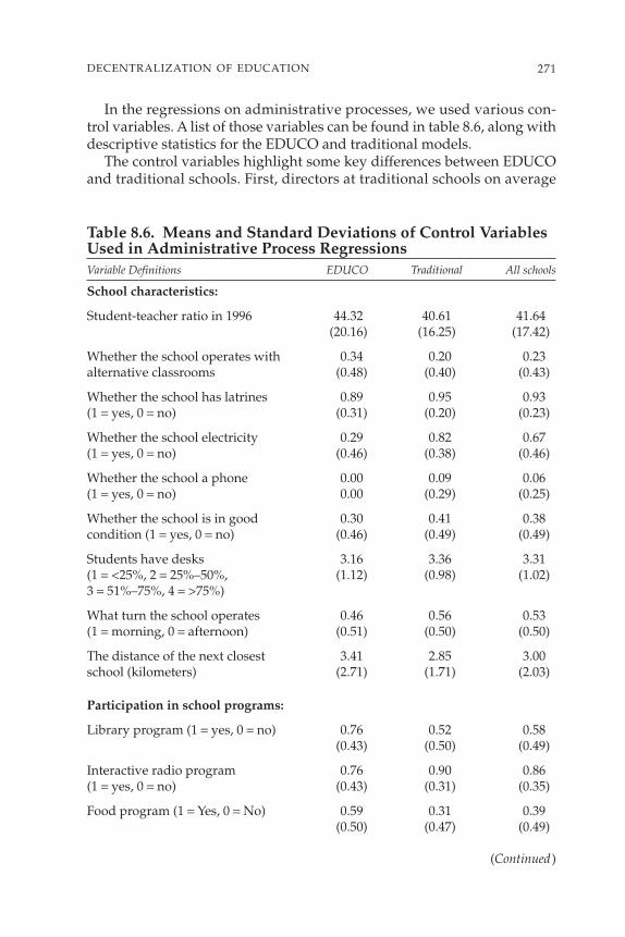
In the regressions on administrative processes, we used various con-trol variables. A list of those variables can be found in table 8.6, along withdescriptive statistics for the EDUCO and traditional models.
The control variables highlight some key differences between EDUCOand traditional schools. First, directors at traditional schools on average
271DECENTRALIZATION OF EDUCATION
Table 8.6. Means and Standard Deviations of Control VariablesUsed in Administrative Process RegressionsVariable Definitions EDUCO Traditional All schools
School characteristics:
Student-teacher ratio in 1996 44.32 40.61 41.64(20.16) (16.25) (17.42)
Whether the school operates with 0.34 0.20 0.23alternative classrooms (0.48) (0.40) (0.43)
Whether the school has latrines 0.89 0.95 0.93 (1 = yes, 0 = no) (0.31) (0.20) (0.23)
Whether the school electricity 0.29 0.82 0.67 (1 = yes, 0 = no) (0.46) (0.38) (0.46)
Whether the school a phone 0.00 0.09 0.06 (1 = yes, 0 = no) 0.00 (0.29) (0.25)
Whether the school is in good 0.30 0.41 0.38 condition (1 = yes, 0 = no) (0.46) (0.49) (0.49)
Students have desks 3.16 3.36 3.31 (1 = <25%, 2 = 25%–50%, (1.12) (0.98) (1.02) 3 = 51%–75%, 4 = >75%)
What turn the school operates 0.46 0.56 0.53 (1 = morning, 0 = afternoon) (0.51) (0.50) (0.50)
The distance of the next closest 3.41 2.85 3.00 school (kilometers) (2.71) (1.71) (2.03)
Participation in school programs:
Library program (1 = yes, 0 = no) 0.76 0.52 0.58(0.43) (0.50) (0.49)
Interactive radio program 0.76 0.90 0.86 (1 = yes, 0 = no) (0.43) (0.31) (0.35)
Food program (1 = Yes, 0 = No) 0.59 0.31 0.39(0.50) (0.47) (0.49)
(Continued)
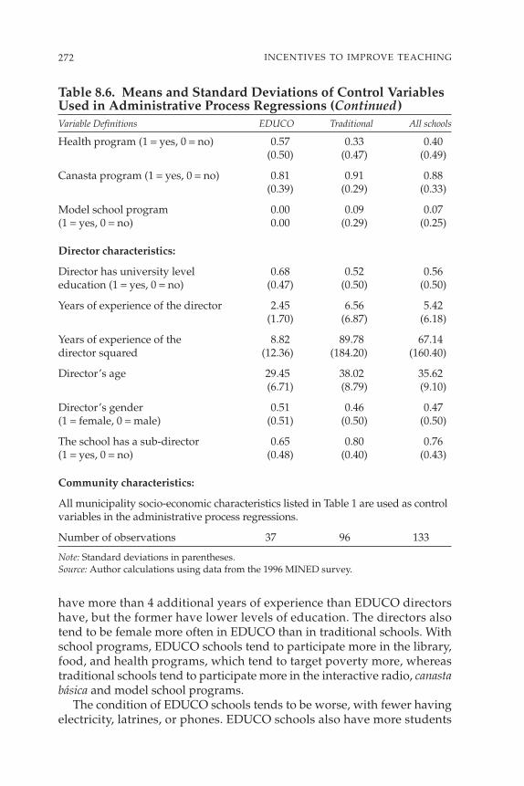
272 INCENTIVES TO IMPROVE TEACHING
Health program (1 = yes, 0 = no) 0.57 0.33 0.40(0.50) (0.47) (0.49)
Canasta program (1 = yes, 0 = no) 0.81 0.91 0.88(0.39) (0.29) (0.33)
Model school program 0.00 0.09 0.07 (1 = yes, 0 = no) 0.00 (0.29) (0.25)
Director characteristics:
Director has university level 0.68 0.52 0.56education (1 = yes, 0 = no) (0.47) (0.50) (0.50)
Years of experience of the director 2.45 6.56 5.42(1.70) (6.87) (6.18)
Years of experience of the 8.82 89.78 67.14 director squared (12.36) (184.20) (160.40)
Director’s age 29.45 38.02 35.62(6.71) (8.79) (9.10)
Director’s gender 0.51 0.46 0.47(1 = female, 0 = male) (0.51) (0.50) (0.50)
The school has a sub-director 0.65 0.80 0.76 (1 = yes, 0 = no) (0.48) (0.40) (0.43)
Community characteristics:
All municipality socio-economic characteristics listed in Table 1 are used as controlvariables in the administrative process regressions.
Number of observations 37 96 133
Note: Standard deviations in parentheses.Source: Author calculations using data from the 1996 MINED survey.
Table 8.6. Means and Standard Deviations of Control VariablesUsed in Administrative Process Regressions (Continued)Variable Definitions EDUCO Traditional All schools
have more than 4 additional years of experience than EDUCO directorshave, but the former have lower levels of education. The directors alsotend to be female more often in EDUCO than in traditional schools. Withschool programs, EDUCO schools tend to participate more in the library,food, and health programs, which tend to target poverty more, whereastraditional schools tend to participate more in the interactive radio, canastabásica and model school programs.
The condition of EDUCO schools tends to be worse, with fewer havingelectricity, latrines, or phones. EDUCO schools also have more students

without desks. Overall subjective rating of school condition reflects thoseresults, with the school condition tending to be lower in EDUCO schools.EDUCO schools tend to be in more isolated areas, with the next-closestschool tending to be farther away.
Although the results are controlled for in the regression analysis, thepoorer conditions of EDUCO schools would most likely have a negativeeffect on administrative processes, as well as on teacher behavior andstudent achievement. In this sense, a downward bias in unobserved vari-ables may exist when measuring the EDUCO effect.
Empirical Results for Administrative ProcessesThe results for administrative processes are broken out into three sepa-rate sections. First, a summary of the results for degree of decentraliza-tion (whether the major influence level is at the school, departmental, ornational level) is given. Second, a summary of the results for percep-tion of own influence for directors, teachers, and school associations ispresented. Third, the main conclusions of the administrative analysisare summarized.
Because of the large number of regressions, the full regression resultscould not be easily shown.113 To focus on one common and importantresult of all the regressions, we presented the OLS coefficient found onthe EDUCO dummy variable, δ, in equation 8.1. In most of the followingtables and figures, we show OLS coefficient of δ and indicate which coef-ficients are statistically significant. To conserve space in the main body ofthis chapter, we focus on only the 10 administrative processes that aremost likely to influence a teacher’s behavior.
DEGREE OF DECENTRALIZATION
The results for the degree of overall decentralization are mixed, with a fairlyeven distribution of positive and negative coefficients. Of the 29 adminis-trative processes, only 7 are statistically significant. Those results on thelevel of decentralization do not confirm the hypothesis that EDUCOschools are more decentralized than traditional schools when measured bymajor influence. For many administrative processes, the major decisionsare still made at the national or departmental level for both EDUCO andtraditional schools.
Figure 8.2 illustrates the OLS coefficient values of the 10 administra-tive processes most likely to affect teacher behavior.
When one looks at administrative processes as a whole, EDUCO schoolsdo not seem much more decentralized when compared with traditionalschools, but one administrative process that could arguably have the most
273DECENTRALIZATION OF EDUCATION
113. Detailed regression results are available from the authors upon request.
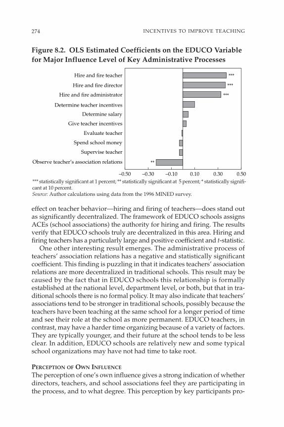
effect on teacher behavior—hiring and firing of teachers—does stand outas significantly decentralized. The framework of EDUCO schools assignsACEs (school associations) the authority for hiring and firing. The resultsverify that EDUCO schools truly are decentralized in this area. Hiring andfiring teachers has a particularly large and positive coefficient and t-statistic.
One other interesting result emerges. The administrative process ofteachers’ association relations has a negative and statistically significantcoefficient. This finding is puzzling in that it indicates teachers’ associationrelations are more decentralized in traditional schools. This result may becaused by the fact that in EDUCO schools this relationship is formallyestablished at the national level, department level, or both, but that in tra-ditional schools there is no formal policy. It may also indicate that teachers’associations tend to be stronger in traditional schools, possibly because theteachers have been teaching at the same school for a longer period of timeand see their role at the school as more permanent. EDUCO teachers, incontrast, may have a harder time organizing because of a variety of factors.They are typically younger, and their future at the school tends to be lessclear. In addition, EDUCO schools are relatively new and some typicalschool organizations may have not had time to take root.
PERCEPTION OF OWN INFLUENCE
The perception of one’s own influence gives a strong indication of whetherdirectors, teachers, and school associations feel they are participating inthe process, and to what degree. This perception by key participants pro-
274 INCENTIVES TO IMPROVE TEACHING
–0.50 –0.30 –0.10 0.10 0.30 0.50
Spend school money
Determine salary
***
***
***
**Observe teacher’s association relations
Supervise teacher
Evaluate teacher
Give teacher incentives
Determine teacher incentives
Hire and fire administrator
Hire and fire director
Hire and fire teacher
*** statistically significant at 1 percent; ** statistically significant at 5 percent; * statistically signifi-cant at 10 percent.Source: Author calculations using data from the 1996 MINED survey.
Figure 8.2. OLS Estimated Coefficients on the EDUCO Variablefor Major Influence Level of Key Administrative Processes

vides a good indication of whether a process is relatively decentralized inEDUCO compared with traditional schools. At the same time, becausethe perspectives are subjective rather than hard data, there is the poten-tial that respondents understood the questions differently or may havehad reason to respond according to what they felt they should say ratherthan their giving a truthful answer. Even looking at the responses with askeptical eye, we see some interesting results emerge.
Figure 8.3 summarizes the results of the perception of own influence fordirector, teacher, and school association for the 10 processes that are mostlikely to influence a teacher’s behavior. The figure illustrates the followingkey findings:
• First, the most striking results of influence come from the school associ-ation responses. Of the 29 questions related to administrative processes,all estimated coefficients were positive, and 26 were statistically sig-nificant (note that determine salary was dropped because almost allresponses were “national”). The reduced graph of the 10 key adminis-trative processes is illustrative of the overall results, indicating thatassociations in EDUCO schools tend to feel that they have significantlymore influence than associations in traditional schools.
275DECENTRALIZATION OF EDUCATION
Hire and fire teacher
Hire and fire administrator
Give teacher incentives
Determine teacher incentives
Evaluate teacher
Spend school money
Determine salary
–1.00 –0.50 0.00 0.50 1.00 1.50 2.00
DirectorTeacherAssociation
***
***
***
**
******
*
****
*****
Observe teacher’s association relations
Supervise teacher
Hire and fire director
*** statistically significant at 1 percent; ** statistically significant at 5 percent; * statistically signifi-cant at 10 percent.Source: Author calculations using data from the 1996 MINED survey.
Figure 8.3. Estimated Coefficients for EDUCO PerceivedAmount of Influence Compared with Traditional Schools

• Second, the results for director influence tend to be negative but are notstatistically significant except for the administrative process of hiring andfiring of director. Those negative coefficients may indicate that directorsin EDUCO schools tend to feel that they have less influence than their tra-ditional counterparts. This finding could be the result of some responsi-bility in administrative processes shifting toward the school associations.
• Third, teacher responses tended to be positive, though often not statis-tically significant, with 16 of the 29 processes having a positive coeffi-cient. This finding brings up an interesting aspect of the EDUCO schoolsystem: although teachers act as agents in the EDUCO structure—withtheir activities being monitored and hiring and firing decisions beingmade by the ACE—the results indicate that teachers in EDUCO schoolsmay also feel that they can influence the processes more than their tra-ditional counterparts.
Addressing Bias IssuesAs mentioned earlier, there is a strong likelihood of selection bias and unobservable variable bias. A few key areas of concern include thefollowing:
• Likelihood of sample selection bias to exist: Because part of the selectionprocess for placement of EDUCO schools includes a demonstrationof interest from the community, EDUCO schools are more likely to beplaced in more-motivated communities. This motivation factor may playan important role in the operation of the school, in teachers’ behavior,and in students’ achievement. This form of bias would result in over-stating the EDUCO effect.
• The newness effect: The fact that EDUCO schools tend to be newer couldcreate both positive and negative unobserved effects. A newer schoolmay receive more attention and care from the community. EDUCOschools, thus, may benefit from what is known as the “Hawthorne”effect—schools that have more recently entered the program have staffand students who are motivated and ready to undertake more reforms.However, this enthusiasm may wane over time.
• Negative aspect of the newness effect: On the flip side, newer schools maystruggle if administrative processes are not well established or if par-ents are not as capable of operating the school. This weakness couldhave a negative effect on teachers’ behavior, administrative process,and, ultimately, students’ achievement.
Many of the control variables that are used will help to capture some ofthose factors, but there is a high likelihood that bias still exists. To check
276 INCENTIVES TO IMPROVE TEACHING
whether the sample selection or unobservable bias is serious, we use twoeconometric methods: propensity score matching114 and Heckman’smodel of endogenous sample selection.115
Results and Interpretation of the Propensity Score and Treatment EffectsThe propensity score and treatment effects model look at the bias issuefrom different angles. In this case, both arrive at the same conclusionthat the OLS model, in general, does not suffer from serious bias. First,the propensity scores are similar to the OLS results. There are a few OLSresults, however, that are statistically significant, but that the propensityscore, treatment-effects model, or both have identified as containingbias.
Two exceptions stand out for the results in level of decentralization.First, the hiring and firing of administration has strong statistical signifi-cance in the OLS model. However, that significance disappears in thepropensity score model, indicating that this administrative process is, infact, not more decentralized in EDUCO schools. Second, the determinationof teacher salaries was not statistically significant using OLS, but itbecomes statistically significant using propensity score matching.
One striking result emerges for the influence results. In the OLS model,teachers had statistically significant results for determining teacher incen-tives and giving teacher incentives. The statistical significance disappearswith propensity score matching. This finding seems to indicate that teachersdo not tend to feel they have more influence in EDUCO schools.
In table 8.7 and table 8.8, in the Heckman two-step model columns, z-stat and λz-stat represent z-statistics of EDUCO coefficient and t-statisticsof λ in the case of the Heckman’s two-step estimation procedure. The treat-ment effects model does not have any statistically significant λz-statisticsfor the decentralization level results, which indicates that the model doesnot suffer from serious sample selection bias. For influence level, three λz
277DECENTRALIZATION OF EDUCATION
114. Propensity score matching helps address the selection bias problem by “correcting”the estimation of treatment effects. It does so by controlling for the existence of unobservedcharacteristics that are based on the idea that the bias is reduced when the comparison ofoutcomes is performed using treated and control subjects who are as similar as possible.
115. To implement this technique, we used the treatment-effects model command, treatreg,using the Heckman two-step option. A critical factor in using the treatreg command is to beable to identify the ingredients that go into deciding which schools receive the treatment(become EDUCO schools). We used community-specific, socioeconomic, and school distancevariables as instruments for the endogenous sample selection for equation 8.5, because thosecharacteristics are used in determining the placement of EDUCO schools. Using this tech-nique, we can determine whether bias exists in our model.
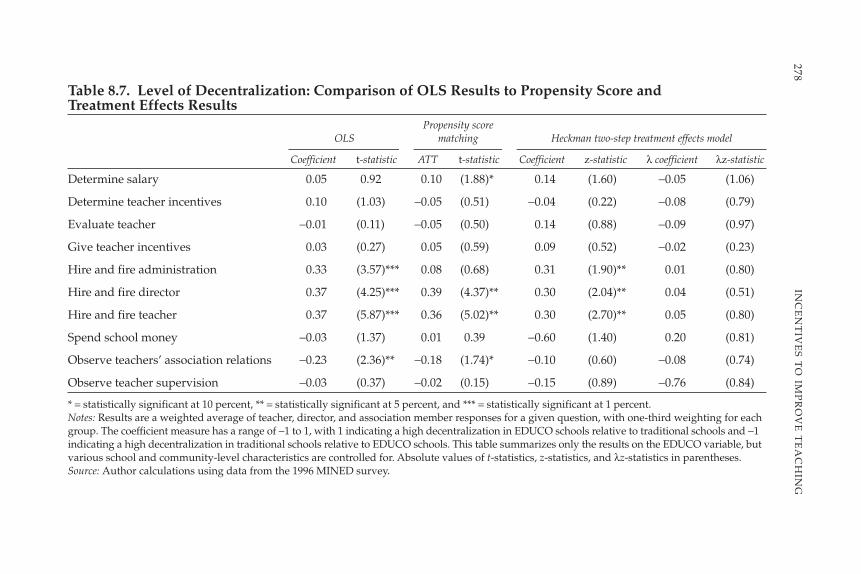
278IN
CE
NT
IVE
ST
OIM
PR
OV
ET
EA
CH
ING
Table 8.7. Level of Decentralization: Comparison of OLS Results to Propensity Score and Treatment Effects Results
Propensity score OLS matching Heckman two-step treatment effects model
Coefficient t-statistic ATT t-statistic Coefficient z-statistic λ coefficient λz-statistic
Determine salary 0.05 0.92 0.10 (1.88)* 0.14 (1.60) −0.05 (1.06)
Determine teacher incentives 0.10 (1.03) −0.05 (0.51) −0.04 (0.22) −0.08 (0.79)
Evaluate teacher −0.01 (0.11) −0.05 (0.50) 0.14 (0.88) −0.09 (0.97)
Give teacher incentives 0.03 (0.27) 0.05 (0.59) 0.09 (0.52) −0.02 (0.23)
Hire and fire administration 0.33 (3.57)*** 0.08 (0.68) 0.31 (1.90)** 0.01 (0.80)
Hire and fire director 0.37 (4.25)*** 0.39 (4.37)** 0.30 (2.04)** 0.04 (0.51)
Hire and fire teacher 0.37 (5.87)*** 0.36 (5.02)** 0.30 (2.70)** 0.05 (0.80)
Spend school money −0.03 (1.37) 0.01 0.39 −0.60 (1.40) 0.20 (0.81)
Observe teachers’ association relations −0.23 (2.36)** −0.18 (1.74)* −0.10 (0.60) −0.08 (0.74)
Observe teacher supervision −0.03 (0.37) −0.02 (0.15) −0.15 (0.89) −0.76 (0.84)
* = statistically significant at 10 percent, ** = statistically significant at 5 percent, and *** = statistically significant at 1 percent.Notes: Results are a weighted average of teacher, director, and association member responses for a given question, with one-third weighting for eachgroup. The coefficient measure has a range of −1 to 1, with 1 indicating a high decentralization in EDUCO schools relative to traditional schools and −1indicating a high decentralization in traditional schools relative to EDUCO schools. This table summarizes only the results on the EDUCO variable, butvarious school and community-level characteristics are controlled for. Absolute values of t-statistics, z-statistics, and λz-statistics in parentheses.Source: Author calculations using data from the 1996 MINED survey.
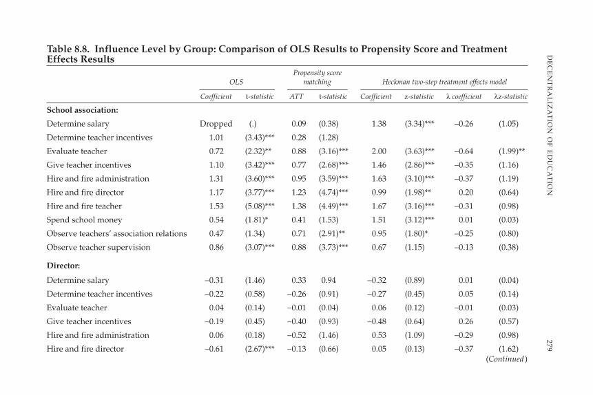
279D
EC
EN
TR
AL
IZA
TIO
NO
FE
DU
CA
TIO
NTable 8.8. Influence Level by Group: Comparison of OLS Results to Propensity Score and TreatmentEffects Results
Propensity score OLS matching Heckman two-step treatment effects model
Coefficient t-statistic ATT t-statistic Coefficient z-statistic λ coefficient λz-statistic
School association:
Determine salary Dropped (.) 0.09 (0.38) 1.38 (3.34)*** −0.26 (1.05)
Determine teacher incentives 1.01 (3.43)*** 0.28 (1.28)
Evaluate teacher 0.72 (2.32)** 0.88 (3.16)*** 2.00 (3.63)*** −0.64 (1.99)**
Give teacher incentives 1.10 (3.42)*** 0.77 (2.68)*** 1.46 (2.86)*** −0.35 (1.16)
Hire and fire administration 1.31 (3.60)*** 0.95 (3.59)*** 1.63 (3.10)*** −0.37 (1.19)
Hire and fire director 1.17 (3.77)*** 1.23 (4.74)*** 0.99 (1.98)** 0.20 (0.64)
Hire and fire teacher 1.53 (5.08)*** 1.38 (4.49)*** 1.67 (3.16)*** −0.31 (0.98)
Spend school money 0.54 (1.81)* 0.41 (1.53) 1.51 (3.12)*** 0.01 (0.03)
Observe teachers’ association relations 0.47 (1.34) 0.71 (2.91)** 0.95 (1.80)* −0.25 (0.80)
Observe teacher supervision 0.86 (3.07)*** 0.88 (3.73)*** 0.67 (1.15) −0.13 (0.38)
Director:
Determine salary −0.31 (1.46) 0.33 0.94 −0.32 (0.89) 0.01 (0.04)
Determine teacher incentives −0.22 (0.58) −0.26 (0.91) −0.27 (0.45) 0.05 (0.14)
Evaluate teacher 0.04 (0.14) −0.01 (0.04) 0.06 (0.12) −0.01 (0.03)
Give teacher incentives −0.19 (0.45) −0.40 (0.93) −0.48 (0.64) 0.26 (0.57)
Hire and fire administration 0.06 (0.18) −0.52 (1.46) 0.53 (1.09) −0.29 (0.98)
Hire and fire director −0.61 (2.67)*** −0.13 (0.66) 0.05 (0.13) −0.37 (1.62)(Continued)

280IN
CE
NT
IVE
ST
OIM
PR
OV
ET
EA
CH
ING
Table 8.8. Influence Level by Group: Comparison of OLS Results to Propensity Score and TreatmentEffects Results (Continued)
Propensity score OLS matching Heckman two-step treatment effects model
Coefficient t-statistic ATT t-statistic Coefficient z-statistic λ coefficient λz-statistic
Hire and fire teacher −0.25 (0.92) −0.37 (1.26) −0.42 (0.96) 0.10 (0.38)
Spend school money 0.07 (0.22) −0.30 (0.96) 0.31 (0.61) −0.16 (0.53)
Observe teachers’ association relations −0.51 (1.30) −0.88 (2.40)** −0.75 (1.12) 0.10 (0.25)
Observe teacher supervision 0.15 (0.43) −0.33 (1.00) −0.09 (0.15) 0.21 (0.59)
Teacher:
Determine salary −0.08 (0.40) 0.16 0.66 0.67 (1.84)* −0.44 (2.08)**
Determine teacher incentives 0.61 (1.89) 0.00 0.01 0.97 (1.88)* −0.19 (0.63)
Evaluate teacher 0.48 (1.53) 0.13 0.35 −0.09 (0.17) 0.31 (0.96)
Give teacher incentives 0.63 (2.18)** 0.21 0.75 −0.54 (0.95) 0.72 (2.23)**
Hire and fire administration −0.17 (0.79) −0.29 (1.17) 0.00 (0.01) −0.11 (0.55)
Hire and fire director −0.26 (1.53) −0.22 (1.05) 0.00 (0.01) −0.16 (0.91)
Hire and fire teacher −0.03 (0.19) 0.14 0.83 0.23 (0.76) −0.15 (0.86)
Spend school money 0.14 (0.40) 0.20 0.55 −0.66 (1.01) 0.53 (1.39)
Observe teachers’ association relations 0.11 (0.27) −0.44 (1.19) 0.38 (0.58) −0.17 (0.45)
Observe teacher supervision 0.43 (1.28) 0.32 0.80 0.08 (0.14) 0.20 (0.60)
* = statistically significant at 10 percent, ** = statistically significant at 5 percent, and *** = statistically significant at 1 percent.Notes: The coefficient measure has a range of −1 to 1, with 1 indicating a high decentralization in EDUCO schools relative to traditional schools and −1indicating a high decentralization in traditional schools relative to EDUCO schools. This table summarizes only the results on the EDUCO variable,but various school and community-level characteristics are controlled for. Absolute values of t-statistics, z-statistics, and λz-statistics in parentheses.Source: Author calculations using data from the 1996 MINED survey.

results are statistically significant: evaluate teacher for school associationand determine salary and give teacher incentives for teacher. In this case, therule is to use the z-statistic and coefficient of the treatment effects modelin place of OLS. The z-statistics for the school association evaluate teacherand teacher determine salary are similar to the OLS result, so no change ismade, but the result for teacher give teacher incentives becomes statisticallyinsignificant.
Overall Conclusion of Administrative ProcessesWhen we compare EDUCO and traditional schools from the perspective ofwhere decisions primarily occur (at the school, departmental, or nationallevel), the overall results suggest that the EDUCO program does notenhance the degree of decentralization as much as might be expected in adecentralization program. Still, significant decentralization does emergein the area of hiring and firing decisions. When comparing EDUCO andtraditional schools from the perspective of perceived influence, much moredistinct differences emerge between the two programs. Actually, associa-tions in EDUCO schools feel they have greater influence than their tradi-tional counterparts. For some of those processes, teachers, directors, andassociation members in EDUCO schools all feel they have more influencethan in traditional schools, signaling more decentralization. For processeswhere associations feel they have more influence, directors tend to feel theyhave less influence. This finding indicates that there may be a reallocationof influence, where associations have been given more power in areas tra-ditionally performed by the director.
The check for sample selection bias using propensity score matchingand the treatment effects model uncovered some areas where the OLSresults appeared to be statistically significant but, in fact, contained sam-ple selection bias, unobservable variable bias, or both. We can be more con-fident that the results that survived both the propensity score and thetreatment effects check capture an “EDUCO effect.”
Of the results that emerged, two points are critical for analysis in thefollowing sections. First, school associations in EDUCO schools do tend tofeel they have significantly more influence in virtually every administrativeprocess. Second, although we did not find it to be the case that all admin-istrative processes have shifted to the school level under the EDUCOmodel, hiring and firing authority does seem to be much more decen-tralized in EDUCO schools. This variable could arguably be the biggestpotential influence on teacher behavior because teachers are closelymonitored by school associations and because teachers realize their con-tract renewal depends on the decision of the school associations. Thosetwo points lead to the argument that EDUCO schools do, in fact, repre-sent a classical principal–agent model, which could address some of
281DECENTRALIZATION OF EDUCATION
the moral hazard and information problems faced by microdevelop-ment programs.116
How Has Decentralization Changed Teachers’ Behavior?
The results from the previous section indicate that EDUCO administra-tive processes show some marked differences from those of traditionalschools. EDUCO associations tend to feel they have more influence inalmost all administrative matters examined. A key administrative processthat could influence teacher behavior—hiring and firing of teachers—seems to be much more decentralized in EDUCO when compared withtraditional schools. With this understanding, what sort of effect does theEDUCO model have on teachers’ behavior?
A comparison of the EDUCO and traditional models presents a classicexample of the principal–agent economic model. The teachers in this caseare the agents. In EDUCO schools, the ACE plays the role of principal,whereas in traditional schools the principal is typically at the departmen-tal or national level. Economic theory suggests that because the principal,who plays a role in evaluating and determining the agent’s incentivesand future employment, is much closer to the agent in the EDUCO modeland can closely monitor the agent’s activities, the agent will be motivatedto work harder. The following section analyzes how the more-decentralizedEDUCO model affects teacher behavior.
The Model of Endogenous Teacher EffortTeachers in EDUCO schools are selected and dismissed according to theirteaching performance by the community associations drawn from theparents of the students (ACEs). Therefore, we can plausibly suppose thatthe “principal” is either the Ministry of Education in traditional schools orthe community association in EDUCO schools, and the “agent” is a teacher.
In El Salvador’s traditional public primary schools, specific governmentregulations (Escalafón Magisterial) ensure a teacher’s job stability, andteachers’ wage levels are determined by MINED (World Bank 1994, 1995).Hence, we can model the teacher wage scheme in traditional schools asbasically a fixed-wage system. In contrast, the ACEs supervise and evalu-ate EDUCO teachers according to their performance (World Bank 1995).Teachers in EDUCO schools receive yearly contracts and their contract
282 INCENTIVES TO IMPROVE TEACHING
116. Moral hazard is the risk that one party to a contract can change his or her behaviorto the detriment of the other party once the contract has been concluded. In this case, themoral hazard is that a teacher who does not feel that poor performance on her or his part willlead to firing (or that good performance will be rewarded) lacks incentive to work hard. Themore secure contract of a traditional school teacher and the inability of the national govern-ment to observe the teacher’s activities could lead to poor performance.

renewal depends on their performance (MINED 1999). Hence, we canplausibly represent that a teacher, particularly an EDUCO school teacher,will be paid according to the “observed” level of teaching effort, which isestimated by the principal. The model constructed in this section followsSawada (1999), who constructed a standard principal–agent model with alinear compensation scheme (Hart and Holmström 1987; Holmström andMilgrom 1991).
If we denote the observed effort level of a teacher as OE, then we canrepresent the teacher payment scheme by a linear function of the observedeffort level as follows:117
where W is the present value of a teacher’s expected wage rate. Note thata2 > 0 denotes a de facto piece-rate contract of EDUCO schools, while acase of a1 > 0 and a2 = 0 can be interpreted as a fixed-wage contract in tra-ditional schools.
The community association can observe an imperfect indicator, OE,of the true teacher effort, e, where OE provides some information aboutthe teacher’s effort but is contaminated by random events beyond thecontrol of the teacher. Formally, we can write
where z indicates a measurement error with E(z) = 0. Although the princi-pal cannot observe e and z separately, a more-involved community asso-ciation allows the observation of teacher effort with higher precisionthrough close and frequent monitoring of a teacher’s behavior. This con-sideration can be represented as var(z) = σz
2, which theoretically is smallerfor EDUCO schools than for traditional schools.118
Suppose that a teacher is risk-averse with the coefficient of absolute riskaversion, γ. Then, we obtain the following incentive compatibility con-straint of a teacher from the first-order condition of a teacher’s utility max-imization problem:
( . )8 10 2aCS e
e= ∂ ( )
∂
( . )8 9 OE e z= +
( . )8 8 1 2W a a OE= +
283DECENTRALIZATION OF EDUCATION
117. Although we can simply interpret the linearity with respect to effort level as anapproximation of a general nonlinear wage-payment formula, the linear compensationscheme is shown theoretically to be adequate and optimal (Hart and Holmström 1987).
118. This variance, V(z), can be interpreted as the inverse of the precision of estimatingteachers’ efforts, thereby reflecting the monitoring technology adopted by the communityassociation.

where the cost created by effort, CS, is assumed to be a convex function ofeffort level, e. Accordingly, we have the optimal level of effort as a functionof the slope of the wage scheme parameter, that is, e* = e (a2), where it iseasily verified that ∂e*/∂a2 > 0.
THE ROLE OF COMMUNITY IN DESIGNING AN OPTIMAL
TEACHER PAYMENT SCHEME
If the community association has full administrative and managementability, the coefficient, a2, is determined endogenously by the communityassociation in order to “discipline” teachers. The community associationwill be concerned with the social benefit of education, which is measuredby a weighted average of students’ educational achievements and of ateacher’s benefit. A community association maximizes the sum of the cer-tainty equivalent incomes of the principal (community association) and theagent (teacher), subject to the incentive compatibility constraint. Then,we obtain the following optimal intensity of incentives condition, that is,the optimal slope of the wage compensation scheme as a function of σz
2
and other parameters (Milgrom and Roberts 1992, pp. 221–23):
where it is easily verified that ∂a2*/∂(σz2) < 0.119
Equation 8.11 indicates the important role of community monitoring.In EDUCO schools, intensive community participation improves the pre-cision of measuring teacher effort. When a teacher’s performance is easyto identify, strong incentives are likely to be optimal. Under the central-ized system, in contrast, community participation is minimal and thusthe precision-of-effort estimation is quite low. When effort measure ishighly imprecise, it is unfruitful to use a wage incentive scheme. As aresult, the fixed teacher compensation scheme in traditional schools canbe rationalized.
Finally, combining equation 8.10 with equation 8.11, we have the opti-mal level of effort as a function of the level of community participation andschool type:
where ∂e*/∂(σz2) < 0. Equation 8.12 represents that in EDUCO schools—
where the precision of monitoring teacher behavior is higher (σz2 is
smaller) than that in traditional schools—teacher effort level is higher. In
( . ) *8 12 2e e g z= ( )[ ]σ
( . ) *8 11 22a g z= ( )σ
284 INCENTIVES TO IMPROVE TEACHING
119. This optimal intensity of incentives condition indicates that the community associa-tion will choose a2 optimally to induce the teacher to set the marginal cost of effort equal to itsmarginal social value of effort.

a typical case, the slope of equation 8.8 is higher for EDUCO schools thanfor traditional schools because EDUCO schools have lower σz
2. From theseresults, we can hypothesize that the level of teacher effort is systematicallyhigher in EDUCO schools than in traditional schools because of the dif-ference in the intensity of community participation. This theoretical gap inthe level of teacher effort suggests the moral hazard problem of teachereffort in traditional schools.
ESTIMATING TEACHER EFFORT
According to equation 8.10, the de facto piece-rate payment scheme inEDUCO schools is thought to enhance teacher effort. Moreover, thechoice of payment scheme should be related to the intensity of communityparticipation according to the optimal intensity of incentives condition(equation 8.11). Hence, the observed level of teacher effort must be a func-tion of the precision of monitoring the teachers’ behavior (equation 8.12).
To investigate this mechanism empirically, we estimated a linearizedversion of the teacher-effort function along with teacher-specific variables.By combining equations 8.9 and 8.12, we have
By linearizing equation 8.13, we get an estimation model of the observedeffort level:
where D is a dummy variable that takes one if the school is an EDUCOschool and zero otherwise, and where X is a set of other control vari-ables. Thus, we focus on the major difference in σz
2 between EDUCO andtraditional schools, because we take the EDUCO dummy as a proxy vari-able for σz
2.In equation 8.14, the observed measure of teacher effort, OE, is not
observed by the econometrician. Therefore, we have used various mea-sures to quantify it. If the estimated coefficient, α1, of equation 8.14 is pos-itive and statistically significant, the finding indicates that—with thehigher degree of community participation—the teacher effort measure inEDUCO schools is better than that in traditional schools. This result can beinterpreted as finding that community participation enhances the teachereffort level, possibly through designing an appropriate wage compensa-tion scheme for teachers.
Moreover, in EDUCO schools, teacher candidates are interviewed byACE. Then ACE determines who is hired on a 1-year contract. Hence,unobserved factors affecting teacher assignments or self-selection toEDUCO schools might be correlated with unobserved factors in determining
( . )8 14 0 1OE D X zj j i j= + + +α α β
( . ) *8 13 2OE e zz= ( ) +σ
285DECENTRALIZATION OF EDUCATION

teacher behavior. This endogeneity of teacher assignments might gener-ate an endogeneity bias if we estimate the model of equation 8.14 by usingOLS. We also model the endogenous assignment of teachers to EDUCOor traditional schools as follows:
where D*S is a latent variable of the propensity of becoming an EDUCO
teacher. As before, we can estimate the model of (8.14), (8.14′), and (8.14″)by using Heckman’s two-step estimation procedure.
Survey Questions Related to Teacher BehaviorTeacher behavior is an abstract concept that is extremely difficult to quan-tify or measure. The survey questions cover behavior that can be measuredto a certain extent and that, although not perfect measures of a teacher’smotivation level, can give an indication of how teachers tend to behaveas a result of working within the different school systems.
To determine what effect the EDUCO program has had on teacher per-formance, we used 19 questions that may provide insights into teacherbehavior and effort. The following is a brief explanation of the data, as wellas an explanation of how it relates to the hypothesis of how monitoringinfluences teacher behavior.
First, a more-motivated teacher would tend to spend more time interact-ing with other members of the school, including students, other teachers, thedirector, and the parents. Hence, we use the following five meeting timevariables to quantify this aspect: separate meeting hours with (a) students,(b) parents, (c) teachers, and (d) a director, plus (e) total meeting hours.
Second, if a teacher is increasingly motivated, she or he might demon-strate an effort by dedicating more time to teaching. Hence, we use threevariables of (a) hours preparing for class, (b) hours grading homework,and (c) hours teaching.
Third, a more-motivated teacher would tend to be more concerned andresponsive when students are not participating in education, includingextended absences. The survey included a question about what the teacherdoes when a student is absent for an extended period of time. Possibleresponses were (a) visiting family, (b) meeting with family, (c) talking tostudents, and (d) talking to the director.
Fourth, a more-motivated teacher would tend to miss fewer days ofschool. Therefore, we include days missed by students because of theteacher’s absence as one of the dependent variables.
( . )*
*8 14
1 0
0 0′′ =
>
<
D
if D
if DS
s
s
i
i
i
( . ) *8 14′ = +D Ws is
s si iγ ν
286 INCENTIVES TO IMPROVE TEACHING
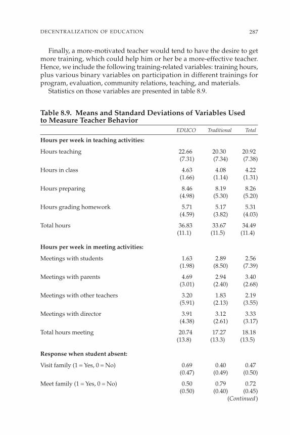
Finally, a more-motivated teacher would tend to have the desire to getmore training, which could help him or her be a more-effective teacher.Hence, we include the following training-related variables: training hours,plus various binary variables on participation in different trainings forprogram, evaluation, community relations, teaching, and materials.
Statistics on those variables are presented in table 8.9.
287DECENTRALIZATION OF EDUCATION
Table 8.9. Means and Standard Deviations of Variables Used to Measure Teacher Behavior
EDUCO Traditional Total
Hours per week in teaching activities:
Hours teaching 22.66 20.30 20.92(7.31) (7.34) (7.38)
Hours in class 4.63 4.08 4.22(1.66) (1.14) (1.31)
Hours preparing 8.46 8.19 8.26(4.98) (5.30) (5.20)
Hours grading homework 5.71 5.17 5.31(4.59) (3.82) (4.03)
Total hours 36.83 33.67 34.49(11.1) (11.5) (11.4)
Hours per week in meeting activities:
Meetings with students 1.63 2.89 2.56(1.98) (8.50) (7.39)
Meetings with parents 4.69 2.94 3.40(3.01) (2.40) (2.68)
Meetings with other teachers 3.20 1.83 2.19(5.91) (2.13) (3.55)
Meetings with director 3.91 3.12 3.33(4.38) (2.61) (3.17)
Total hours meeting 20.74 17.27 18.18(13.8) (13.3) (13.5)
Response when student absent:
Visit family (1 = Yes, 0 = No) 0.69 0.40 0.47(0.47) (0.49) (0.50)
Meet family (1 = Yes, 0 = No) 0.50 0.79 0.72(0.50) (0.40) (0.45)
(Continued)

The measures of teacher behavior are certainly not ideal measures andmust be looked at in context. First, the responses were given by the teachersthemselves. The responses may be subjective or the teacher may attempt togive the response that she or he believes is best to give. Very often theresponses are on an amount of time spent over a given period. It is unlikelythat teachers keep precise records, so there is a risk that the answers are notcompletely accurate. One exception is the measure of a teacher’s absence, forwhich parents say how often their children miss school because the teacheris absent. This response is potentially more objective, but parents may notkeep accurate records of actual days of absence.
288 INCENTIVES TO IMPROVE TEACHING
Talk to student’s friends (1 = Yes, 0 = No) 0.92 0.93 0.93(0.27) (0.25) (0.25)
Talk to the Director (1 = Yes, 0 = No) 0.62 0.74 0.71(0.49) (0.44) (0.45)
Teacher absence according to parent
Days of school missed due to teacher absence 1.19 1.40 1.35(1.15) (1.43) (1.36)
Training variables:
Training hours 7.77 9.12 8.77(11.2) (12.1) (11.9)
Training—program 0.86 0.69 0.73(0.35) (0.46) (0.44)
Training—evaluation 0.91 0.95 0.94(0.28) (0.22) (0.23)
Training—community relations 0.63 0.41 0.47(0.49) (0.49) (0.50)
Training—materials 0.60 0.43 0.48(0.49) (0.49) (0.50)
Training—teaching 0.79 0.64 0.68(0.84) (0.74) (0.77)
Total observations 35 99 134
Note: Standard deviations in parentheses.Source: Author calculations using data from the 1996 MINED survey.
Table 8.9. Means and Standard Deviations of Variables Used toMeasure Teacher Behavior (Continued)
EDUCO Traditional Total
But the argument can also be made that because EDUCO and traditionalteachers have no reason to give different answers (that is, one should notexaggerate more than the other), then the overall results should give a fairlyreasonable picture of level of effort and motivation.
Control Variables Used in RegressionsThe analysis controlled for various teacher, school, and community charac-teristics. Table 8.10 gives descriptive statistics of the control variables used.
Results of Empirical AnalysisThe OLS results for teacher behavior are presented in table 8.11. A num-ber of teacher behavior measures tend to indicate that there may be anEDUCO effect on teacher behavior. When addressing bias issues throughpropensity score matching and Heckman two-step procedures, some ofthe statistically significant OLS results are weeded out, but many statisti-cally significant results remain.
Addressing Bias IssuesWe estimated the model by considering possibilities of the endogenoussample selection. Here, we explicitly model a teacher’s choice of EDUCOor traditional schools by a system of equations 8.14, 8.14′, and 8.14″. Weestimate this model by using Heckman’s two-step procedure. Estimationresults are represented in table 8.11. Most of the z-statistics of the sampleselection coefficient, λ, are not statistically significant. This finding indi-cates that potential bias generated by endogeneity of teacher assignmentsis not serious. Two exceptions are the school program and the commu-nity relations training. For these variables, the λ is statistically significant,indicating that we should use the Heckman result rather than the OLS. TheEDUCO dummy variables for those measures are statistically significantusing OLS but become insignificant under Heckman.
In running the propensity score matching, we were unfortunately notable to get results using our full regression. Because we used 42 differentcontrol variables and had a total of only 134 observations with Stata,120 ourresults were unable to satisfy the balancing check in order to do nearest-neighbor matching. Although we believe this problem is caused by thelarge number of control variables used, we must also consider the possi-bility that Stata could not find neighbors because the control and treatmentgroups are too different. In running the regression after removing 10 of whatseemed to be the least-important control variables and leaving the 32 mostimportant, Stata was able to complete the nearest-neighbor matching. Thisoption is certainly second-best, but we considered that having imperfectresults will give more insight than having no results.
289DECENTRALIZATION OF EDUCATION
120. Stata is a statistical analysis program that was used in performing the regressionanalysis for this study.

290 INCENTIVES TO IMPROVE TEACHING
Table 8.10. Means and Standard Deviations of Control VariablesUsed in Teacher Behavior RegressionsVariable definitions EDUCO schools Traditional schools All schools
Teacher characteristics:
Years of experience 3.91 9.46 8.01(2.64) (7.05) (6.66)
Years of experience squared 22.14 138.86 108.37(29.68) (216.18) (193.15)
Years of experience at school 2.17 6.17 5.15 where currently teaching (1.29) (5.69) (5.24)
Teacher who has a university 0.74 0.30 0.41 education level (1 = yes, 0 = no) (0.44) (0.46) (0.49)
Wage of teacher (salary and bonus) 3,815.00 4,002.00 3,947.00(251.00) (559.00) (494.00)
One who teaches in alternative 0.35 0.19 0.23classroom (1 = yes, 0 = no) (0.48) (0.39) (0.42)
Number of students in classroom 20.80 28.00 26.10(7.71) (11.10) (10.80)
Teacher’s age 27.37 34.41 32.57(4.47) (7.83) (7.74)
Teacher who has class in morning 1.62 1.46 1.50 (1 = morning, 0 = afternoon) (0.49) (0.50) (0.50)
Teacher’s gender 1.37 1.27 1.29 (1 = female, 0 = male) (0.49) (0.44) (0.45)
Teacher’s residence 2.68 2.46 2.52(1 = town, 2 = different town in (1.05) (0.95) (0.97)municipality, 3 = other municipality but same department, 4 = other department)
Time it takes to commute to school 2.08 2.10 2.09 (1 = 30 min, 2 = 30 min−1 hour, (0.88) (0.82) (0.83) 3 = more than 1 hour)
Frequency of commute to school 1.28 1.12 1.16per week (1 = daily, 2 = weekly) (0.45) (0.32) (0.37)
Incentives received by teacher in past year:
Diploma (1 = yes, 0 = no) 0.31 0.16 0.20(0.47) (0.36) (0.40)
Raise (1 = yes, 0 = no) 0.00 0.16 0.110.00 (0.36) (0.32)
(Continued)

291DECENTRALIZATION OF EDUCATION
Scholarship (1 = yes, 0 = no) 0.02 0.02 0.02(0.16) (0.14) (0.14)
Economic (1 = yes, 0 = no) 0.14 0.11 0.11(0.35) (0.31) (0.32)
Benefits received by teacher:
Life insurance (1 = yes, 0 = no) 0.57 0.90 0.82(0.50) (0.28) (0.38)
Medical (1 = yes, 0 = no) 1.00 0.93 0.950.00 (0.23) (0.20)
Vacation (1 = yes, 0 = no) 0.94 0.94 0.94(0.23) (0.22) (0.22)
Housing (1 = yes, 0 = no) 0.88 0.80 0.82(0.32) (0.39) (0.37)
School characteristics:
School is part of library program 0.74 0.48 0.55 (1 = yes, 0 = no) (0.44) (0.50) (0.49)
School is part of interactive radio 0.62 0.79 0.75 program (1 = yes, 0 = no) (0.49) (0.40) (0.43)
School is part of Canasta program 0.74 0.84 0.82(1 = yes, 0 = no) (0.44) (0.36) (0.38)
School is part of food program 0.54 0.35 0.40(1 = yes, 0 = no) (0.50) (0.48) (0.49)
School is part of health program 0.57 0.31 0.38 (1 = yes, 0 = no) (0.50) (0.46) (0.48)
School is part of model school 0.00 0.12 0.08 program (1 = yes, 0 = no) 0.00 (0.32) (0.28)
Number of visits per month by 3.85 4.72 4.50 departmental director (6.76) (6.63) (6.65)
Community characteristics:
All municipality socioeconomic characteristics listed in table 8.1 are used as con-trol variables in the administrative process regressions.
Number of observations 35 99 134
Note: Standard deviations in parentheses.Source: Author calculations using data from the 1996 MINED survey.
Table 8.10. Means and Standard Deviations of Control VariablesUsed in Teacher Behavior Regressions (Continued)Variable definitions EDUCO schools Traditional schools All schools

292IN
CE
NT
IVE
ST
OIM
PR
OV
ET
EA
CH
ING
Table 8.11. Comparison of OLS Results to Treatment Effects and Propensity Score Matching ResultsOriginal OLS with Revised OLS with 32 Propensity score with
42 dependent variables Heckman two-step procedure dependent variables 32 dependent variables
Output variable Coefficient t-statistic Coefficient z-statistic λ coefficient λz-statistic Coefficient t-statistic Coefficient t-statistic
Meeting time (hours/week):
With students −1.07 (0.78) −0.92 (0.40) 0.03 (0.02) −0.45 (0.48) −1.65 (0.50)
With parents 2.20 (2.44)** 4.25 (0.53) −0.92 (0.78) 2.31 (3.53)*** 1.97 (2.10)**
With other teachers 4.24 (2.21)** 5.65 (1.76)* −0.96 (0.46) 2.87 (2.23)** 1.09 (1.48)
With director 1.26 (0.79) 3.97 (1.20) −1.59 (0.89) 2.15 (1.96)* −1.24 (1.38)
Total meeting time 13.12 (1.99)** 22.27 (2.33)** −6.32 (0.77) 11.29 (2.48)** 1.42 (0.29)
Teaching activities (hours/week):
Classroom teaching 3.06 (0.91) 10.13 (1.84)* −4.70 (1.09) 3.51 (1.31) 5.79 (1.91)**
Preparation for class 1.49 (0.66) −4.75 (0.67) 3.04 (1.16) 0.75 (0.46) 1.95 (0.99)
Grade homework 2.18 (1.35) −0.36 (0.08) 1.69 (0.94) 1.54 (1.30) 1.93 (1.21)
Total hours 6.73 (1.49) 5.01 (1.19) 0.02 (0.00) 5.80 (1.52) 9.66 (2.29)**
Response to student absence:
Visit family −0.04 (0.12) −0.81 (1.40) 0.50 (1.63) 0.19 (0.77) 0.27 (1.63) (1 = yes, 0 = no)
Meet family −0.32 (1.02) 0.11 (0.73) −0.10 (0.39) −0.14 (0.65) −0.08 (0.54)(1 = yes, 0 = no)

293D
EC
EN
TR
AL
IZA
TIO
NO
FE
DU
CA
TIO
N
Talk to friends 0.15 (0.78) 0.69 (0.70) −0.26 (1.49) 0.10 (0.83) 0.12 (1.62)(1 = yes, 0 = no)
Visit director −0.07 (0.22) 0.20 (0.42) −0.08 (0.29) 0.03 (0.17) −0.30 (1.99)* (1 = yes, 0 = no)
Teacher absence:
Days missed −1.37 (1.95)** −0.51 (0.64) −0.55 (0.63) −1.12 (2.26)** −0.79 (1.86)*
Training:
Total hours 2.99 (0.48) 7.94 (1.67)* −3.89 (0.54) 4.23 (1.03) −3.91 (0.87)
School program 0.36 (1.74)* −0.44 (1.25) 0.52 (1.88)* 0.47 (3.56)*** 0.44 (3.12)***(1 = yes, 0 = no)
Evaluation 0.13 (1.31) 0.43 (2.02)** −0.20 (1.63) 0.07 (0.94) 0.02 (0.29)(1 = yes, 0 = no)
Community relations 0.38 (1.67)* −0.49 (1.20) 0.52 (1.76)* 0.33 (2.02)** 0.37 (2.15)** (1 = yes, 0 = no)
Materials 0.48 (2.14)** 0.36 (0.11) 0.08 (0.31) 0.38 (2.32)** 0.24 (1.34) (1 = yes, 0 = no)
Teaching 0.32 (0.83) 0.46 (0.29) −0.37 (0.81) −0.14 (0.61) −0.52 (1.94)* (1 = yes, 0 = no)
* = statistically significant at 10 percent, ** = statistically significant at 5 percent, and *** = statistically significant at 1 percent.Notes: The reduced OLS contains the same control variables as the original OLS, except for health program, Canasta program, model school program,transit frequency, life insurance benefits, vice director, municipal mortality, municipal percent rural, phone, electricity, and latrine. Absolute values oft-statistics, z-statistics, and λz-statistics in parentheses.Source: Author calculations using data from the 1996 MINED survey.

The results for propensity score matching indicate that there is bias in theOLS results for a few measures. The measures of meeting with other teach-ers, meeting with the director, total meeting time, and teaching materialstraining were statistically significant under OLS but were insignificant withpropensity score matching. Conversely, the results for time teaching totalhours and for student absent—talk to director were insignificant usingOLS, but become significant under propensity score matching.
So what are we left with? For meeting time, some statistically significantOLS meeting variables become only marginally significant, but the mea-sure of meeting with parents remains strong through all tests. EDUCOteachers do tend to dedicate more time to meetings.
The strong statistical significance that emerges for time dedicated to teach-ing (particularly with propensity score matching) indicates that teachersmay also dedicate more time to teaching. The propensity score results havea coefficient indicating 9.7 hours more per week.
The teacher absence variable also stays statistically significant throughall tests, indicating that EDUCO teachers may be absent less than tradi-tional school teachers. Because teacher absence is a big issue in rural com-munities and can potentially have a negative effect on students’ learning,this result is important.
A few statistically significant results emerge about how the teacherresponds to a student’s extended absence, but those results seem invalid.For example, while one teacher may answer that she or he visits the student’sfamily, another may respond that she or he talks to the director. Is onereally better than the other? Because no strong differences emerged in thisarea, it seems better not to draw any conclusions from the results.
Finally, with respect to training, although OLS had many statisticallysignificant results indicating that EDUCO teachers are more motivated toget training, the Heckman and propensity score matching results indicatethat they are, in fact, not statistically significant. No strong differencesemerge in the area of training.
Overall Conclusions on Teacher BehaviorAs mentioned earlier, the measures used here for teacher behavior areimperfect indicators because behavior and motivation are difficult con-cepts to capture statistically and because it is difficult to know whetherresponses to questions asking amount of time dedicated to activities actu-ally are accurate. Those limitations should be kept in mind, but some inter-esting results do emerge, indicating that teacher behavior and motivationmay be influenced by differences between the EDUCO and traditionalschool programs.
Simple OLS showed many statistically significant results, all indicat-ing that EDUCO teachers are more motivated and active than teachers intraditional schools. Some of the results proved to be caused by sample
294 INCENTIVES TO IMPROVE TEACHING

selection or unobservable bias, but many key measures survived the biastests, including meeting with parents, teacher absence, and hours dedi-cated to teaching.
Although we have to be careful not to jump to conclusions, the resultsindicate that community participation seems to enhance the teacher effortlevel, possibly because of intensive monitoring of teacher behaviors andthe implicit threat that exists because hiring and firing of teachers occurs atthe community level. The measures used are directly observable to bothteachers and parents by nature. Thus, teachers might be interested inimproving them. Close teacher monitoring by communities rather than byexternal supervisors can be less costly than teacher evaluations by externalsupervisors. Even in a small rural school with only one teacher, frequentand close teacher monitoring becomes possible if the supervisor is drawnfrom the same community.
Moreover, teachers may become accountable to the community groupthat monitors, supervises, and evaluates their performance. Accordingly,when members of the community association are elected from the parents ofthe students, inconsistency between the teachers’ behavior and the welfareobjective of the beneficiaries is likely to disappear. Community participa-tion not only uses relevant information that outside government agenciesare not likely to have, but also imposes commitment on teachers, whichleads them to exert greater effort.
How Do Differences in Teacher Behavior Affect Student Achievement?
Although the previous analysis helps to shed light on the effects of decen-tralization on teacher behavior, the second-order effects on studentachievement and learning are not necessarily clear. We would expect thatpositive teacher behavior would result in positive student outcomes. Inpractice, this link is extremely difficult to establish. Our teacher behaviormeasures—such as time spent meeting with parents and other teachers,decreased teacher absence, and working hours—are not perfect measuresof teacher behavior and can at best be linked tentatively to student out-come. If we think of the teacher behavior variables as representing themore-general unobservables of teacher behavior, however, and of a teacherdemonstrating those observable characteristics as being more likely to bemotivated, we can attempt to link teacher behavior and student outcomes.Although imperfect, this approach may shed some light on teacher behav-ior and student outcome.
In an attempt to get a complete picture of this link, we approach ouranalysis from various angles. First, we estimate student outcomes—as mea-sured by student absence and student test scores in math and Spanish—without including teacher behavior variables but controlling for child and
295DECENTRALIZATION OF EDUCATION

household characteristics. (Those control variables can be found in table 8.2.)Then we bring in teacher behavior characteristics. We use some character-istics that emerged as statistically significant in the previous section—teacher absence, teacher working hours, and teacher meeting time withparents. Those variables are first treated as exogenous and then as endoge-nous. By looking at student achievement from the different angles, we hopeto capture the effects of teacher behavior on student outcomes. In all cases,the EDUCO dummy is included to separate the interaction betweenEDUCO and teacher behavior, as well as to separate the teacher behavioreffect from the program effects.
Measure of Student AchievementFor measurement of student outcomes, the achievement tests for varioussubjects were applied by MINED in October 1996 with the assistance of theIntercultural Center for Research in Education (MINED 1997). The testswere applied nationally in the third, fourth, and sixth grades. We use thethird-grade results, and we focus only on the results for the mathematicsand Spanish tests in the analysis.121
According to table 8.12, the average student was able to master 3.70 outof 10 subjects in mathematics, but only 1.75 out of 9 in languages. Theresults are comparable to national averages (MINED 1997). BetweenEDUCO and traditional schools, no statistically significant difference existsin the test scores in spite of the poorer background of EDUCO students.This finding suggests an advantage for community participation in educa-tion. In days of child absence, there is no difference between EDUCO andtraditional schools.
The Model of Teacher Behavior Effects on Educational OutcomesTo examine the complex interaction in the schooling process of the behav-iors of various agents such as students, groups of parents, teachers, andadministrators in creating educational output (Glewwe 2002; Hanushek1995), we use a reduced-form of an education production function. Withrespect to the output measure, we focus on student scores on standardizedachievement tests.122 Suppose that the educational achievement, Qij, of achild i, who is studying at a school j in municipality m, can be representedby the following production function:123
296 INCENTIVES TO IMPROVE TEACHING
121. The mathematics test is composed of 30 questions on 10 key subjects—that is, threeitems for each subject. A student passed a subject if she or he answered two out of three ques-tions right. For the Spanish test, there are 36 questions on nine subjects—that is, four itemseach. A student has passed a subject if she or he answered three out of four questions right.
122. Most studies measure educational output by students’ achievement scores, schoolattendance rates, repetition rates, and school continuation or dropout rates, which arethought to capture prospects of future earnings in the labor market (Hanushek 1995).
123. Gaynor and Pauly (1990) called this function the “efficient” or “maximum (observed)effort” production function.
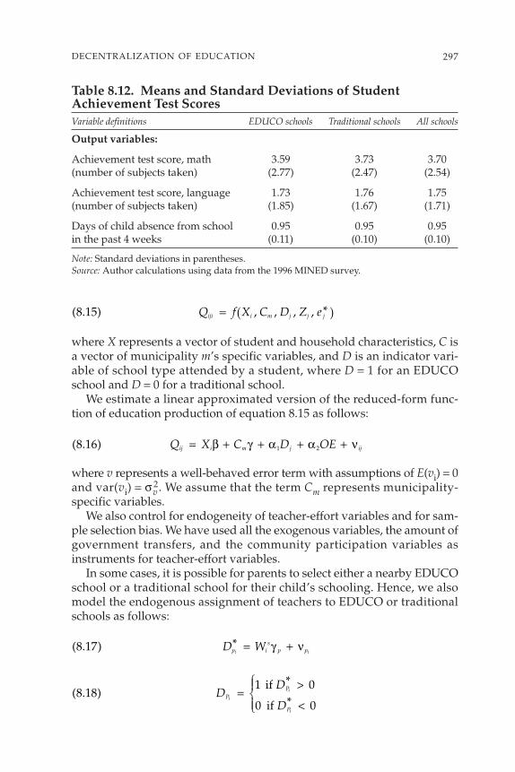
where X represents a vector of student and household characteristics, C isa vector of municipality m’s specific variables, and D is an indicator vari-able of school type attended by a student, where D = 1 for an EDUCOschool and D = 0 for a traditional school.
We estimate a linear approximated version of the reduced-form func-tion of education production of equation 8.15 as follows:
where v represents a well-behaved error term with assumptions of E(vi) = 0and var(vi) = σv
2. We assume that the term Cm represents municipality-specific variables.
We also control for endogeneity of teacher-effort variables and for sam-ple selection bias. We have used all the exogenous variables, the amount ofgovernment transfers, and the community participation variables asinstruments for teacher-effort variables.
In some cases, it is possible for parents to select either a nearby EDUCOschool or a traditional school for their child’s schooling. Hence, we alsomodel the endogenous assignment of teachers to EDUCO or traditionalschools as follows:
( . )*
*8 18
1 0
0 0D
D
DP
P
P
i
i
i
=>
<
if
if
( . ) *8 17 D Wp is
p pi i= +γ ν
( . )8 16 1 2Q X C D OEij i m j ij= + + + +β γ α α ν
( . ) , , , , *8 15 Q f X C D Z eiji i m j j j= ( )
297DECENTRALIZATION OF EDUCATION
Table 8.12. Means and Standard Deviations of StudentAchievement Test ScoresVariable definitions EDUCO schools Traditional schools All schools
Output variables:
Achievement test score, math 3.59 3.73 3.70 (number of subjects taken) (2.77) (2.47) (2.54)
Achievement test score, language 1.73 1.76 1.75 (number of subjects taken) (1.85) (1.67) (1.71)
Days of child absence from school 0.95 0.95 0.95 in the past 4 weeks (0.11) (0.10) (0.10)
Note: Standard deviations in parentheses.Source: Author calculations using data from the 1996 MINED survey.

where D*Pi is a latent variable of the propensity of selecting an EDUCO
school. As before, we estimate the model of equations 8.16, 8.17, and 8.18by using Heckman’s two-step estimation procedure to control for schoolselection of students (parents). For the selection equation, we have usedhousehold and school characteristics, as well as densities of EDUCO andtraditional schools as identifying instruments.
Results of the Empirical AnalysisTables 8.13, 8.14, and 8.15 represent the estimation results of productionfunction 16 for mathematics test score, Spanish test score, and days ofabsence, respectively. All tables contain the following four different speci-fications. In specification 1, we use the propensity score matching method.In specification 2, we estimate the model without teacher behavior vari-ables, controlling for the child and household characteristics in table 8.2. Inspecification 3, we treat two variables as exogenous, and we control for
298 INCENTIVES TO IMPROVE TEACHING
Table 8.13. Estimated EDUCO Effects on Mathematics ScoresSpecification 1 Specification 2 Specification 3a Specification 4b
Coefficient Coefficient Coefficient Coefficient (z-statistic) (z-statistic) (z-statistic) (z-statistic)
Sample Sample Sample selection (2 stage)
Propensity selection selection instrumental Estimation method score (2 stage) (2 stage) variable
Coefficients on:
EDUCO dummy 0.165 0.253 0.04 0.447(0.401) (0.19) (0.03) (0.21)
Teacher’s absence 0.039 0.052days (past 2 weeks) (0.75) (0.03)
Working hours 0.214 −0.235(per day) (1.90)* (0.13)
Hours meeting with 0.06 0.569parents (per month) (0.95) (1.67)*
Lambda −0.342 −0.305 −0.631
(0.42) (0.38) (0.52)
* = statistically significant at 10 percentNote: Absolute values of t-statistics reported in parentheses.a. Specification 3: Treating three variables of teacher behavior as exogenous and controllingfor child and household characteristics.b. Specification 4: Treating three variables of teacher behavior as endogenous and controllingfor child and household characteristics.Source: Author calculations using data from the 1996 MINED survey.

child and household characteristics listed in tables 8.2 and 8.3. Finally, inspecification 4, we treat two variables as endogenous, controlling for childand household characteristics in tables 8.2 and 8.3.
According to tables 8.13, 8.14, and 8.15, most of the coefficients are inline with our theoretical predictions, but the results are not particularlystrong. The Spanish score findings in table 8.14 do have some strong resultswhere the coefficients that are based on the sample selection methods areall statistically significant. There seem to be positive EDUCO effects, a partof which can be explained by positive effects of teacher effort on educa-tional outputs. The results for mathematics and Spanish test scores that arebased on specification 4 show the statistically significant positive effectsof teacher–parent meetings. The results tend to support the theoreticalhypothesis that EDUCO program governance leads to better effort ofteachers, which improves educational outcome, even after controlling forobserved student, household, and community characteristics, as well as
299DECENTRALIZATION OF EDUCATION
Table 8.14. Estimated EDUCO Effects on Spanish ScoresSpecification 1 Specification 2 Specification 3a Specification 4b
Coefficient Coefficient Coefficient Coefficient (z-statistic) (z-statistic) (z-statistic) (z-statistic)
Sample Sample Sample selection (2 stage)
Propensity selection selection instrumental Estimation method score (2 stage) (2 stage) variable
Coefficients on:
EDUCO dummy 0.021 2.481 2.357 2.498(0.081) (2.71)** (2.57)** (1.78)*
Teacher’s absence −0.042 0.159 days (past 2 weeks) (1.15) (0.12)
Working hours (per day) 0.074 0.159(0.94) (0.12)
Hours meeting with 0.027 0.457 parents (per month) (0.60) (1.93)**
Lambda −1.331 −1.303 −1.528(2.49)** (2.43)** (2.00)**
* = statistically significant at 10 percent, and ** = statistically significant a 5 percent.Note: Absolute values of t-statistics reported in parentheses.a. Specification 3: Treating three variables of teacher behavior as exogenous and controllingfor child and household characteristics.b. Specification 4: Treating three variables of teacher behavior as endogenous and controllingfor child and household characteristics.Source: Author calculations using data from the 1996 MINED survey.

possible endogeneity and sample selection biases. Yet, we do not obtainrobust results for the statistical significance. Particularly, the propensityscore matching estimations do not give us significant results. Hence, thefindings are only suggestive and are by no means conclusive.
As for sample selection aspects, we observe a significantly negative sam-ple selection at the student or household level in the case of the Spanish testscores (table 8.14). These negative coefficients suggest that those whoselect EDUCO schools have unobserved characteristics that lead to sys-tematically lower Spanish test scores. Poor family background of EDUCOstudents might be captured by these negative coefficients.
Conclusions
In this chapter, we investigated the effects of decentralization of an educa-tion program by closely examining the example of El Salvador’s EDUCOprogram, which was designed to rapidly expand rural education follow-ing the country’s civil war. Our focus was on how decentralization altersadministration processes and teacher behavior and how those changesmight affect the quality of education.
300 INCENTIVES TO IMPROVE TEACHING
Table 8.15. Estimated Effects on Days of AbsenceSpecification 1 Specification 2 Specification 3a Specification 4b
Coefficient Coefficient Coefficient Coefficient (z-statistic) (z-statistic) (z-statistic) (z-statistic)
Sample Sample Sample selection (2 stage)
Propensity selection selection instrumental Estimation method score (2 stage) (2 stage) variable
Coefficients on:
EDUCO dummy 0.021 −0.896 −0.766 −0.201(0.081) (0.86) (0.73) (0.18)
Working hours (per day) −0.111 −0.640(1.27) (1.30)
Hours meeting with −0.043 0.018 parents (per month) (0.83) (0.14)
Lambda −0.321 0.299 0.102(0.51) (0.47) (0.18)
Note: Absolute values of t-statistics reported in parentheses.a. Specification 3: Treating three variables of teacher behavior as exogenous and controllingfor child and household characteristics.b. Specification 4: Treating three variables of teacher behavior as endogenous and controllingfor child and household characteristics.Source: Author calculations using data from the 1996 MINED survey.

We compared administrative activities and teacher behavior in EDUCOschools with those activities and behaviors in traditional schools, control-ling for characteristics of school, community, and school participants(teacher, director, and student). We also attempted to control for sampleselection bias, using an exogenously determined formula for targetingEDUCO schools as an instrumental variable. As an additional step inaddressing bias issues, we also used propensity score matching techniquesto evaluate the EDUCO program effects.
The results indicate that, interestingly, most of administrative processesin EDUCO schools have not yet shifted to the local level. Nevertheless,selective administrative activities, such as hiring and firing decisions, dodiffer significantly between EDUCO and traditional schools. A large dif-ference is seen when observing perceptions of amount of influence. Keyplayers in the EDUCO schools—especially school associations—tend tofeel they have greater influence in many of the administrative activities.
The results also indicate that decentralization has possibly had a positiveeffect on teacher behavior. Although some results that seemed statisticallysignificant under the OLS model disappeared when other techniques wereused to control for sample selection and unobservable bias, many key mea-sures survived. There are indications that EDUCO teachers may have moremotivation, as measured (a) by spending more time meeting with parentsand other school members, (b) by being absent less, and (c) by dedicatingmore time to teaching. Although it is difficult to directly link teacher moti-vation and student outcomes, the increased motivation may have had apositive effect on student performance. Such results indicate that decen-tralized management programs, when designed correctly, may be able toprovide an incentive structure that leads to greater teacher motivation andperformance.
Policymakers should consider three important issues carefully whenthey apply our analysis in practice. First, the optimal form of community-managed development programs is specific to the development level of acountry (Conning and Kevane 2002, p. 389).
Second, we should resist the temptation to romanticize the value of thelocal community as a social and economic organization (Bardhan andUdry 1999). In reality, mere decentralization does not guarantee the suc-cessful community-based management. One of the more serious prob-lems lies in program implementation caused by a distant, uncoordinated,and corrupt bureaucracy (Bardhan and Udry 1999, pp. 149–50). In thatcase, even if the government aims at allocating its budget to alleviatepoverty, aid does not reach the real poor. Moreover, the superior infor-mation and monitoring technologies in the hands of communities alsomeans that there are potential information rents to be captured (Conningand Kevane 2002, p. 383). Therefore, there is a risk that the local rich can“capture” the local community institutions (Reinikka and Svensson 2004).
301DECENTRALIZATION OF EDUCATION

Finally, regarding efficiency, there could be a major tradeoff between theneed for central policy coordination because of externalities or scaleeconomies and the need for local information and accountability (Bardhan2002, p. 190). With externalities across communities, decentralization leadsto underprovision of public goods. With strong economies of scale, thecentral government can play an important role. For example, it is better tolet the government construct infrastructure such as electric power genera-tion and telecommunication facilities. In primary education, the govern-ment has an absolute advantage in designing curricula and in preparingtextbooks. But as the results of this study suggest, decentralization of cer-tain education management functions has advantages over a centralizedmodel and can have positive effects on important factors such as teacherbehavior and student performance.
In any case, further research on this theme should be directed towardmodeling the complicated incentive problems in micro-development pro-grams to derive structures of appropriate governance of such programs.At the same time, serious efforts should be made in evaluating the effect ofvarious ongoing experiments of micro-development programs by usingmicro data.
302 INCENTIVES TO IMPROVE TEACHING

References
Amemiya, T. 1985. Advanced Econometrics. Cambridge, Mass.: HarvardUniversity Press.
Angrist, J. 1999. “Estimation of Limited Dependent Variable Models withDummy Endogenous Regressors: Simple Strategies for Empirical Prac-tice.” Journal of Business and Economic Statistics 19(1): 2–16.
Angrist, J., E. Bettinger, E. Bloom, E. King, and M. Kremer. 2002. “Vouch-ers for Private Schooling in Colombia: Evidence from a RandomizedNatural Experiment.” American Economic Review 92(5): 1535–58.
Bardhan, P. 2002. “Decentralization of Governance and Development.”Journal of Economic Perspectives 16(4): 185–205.
Bardhan, P., and C. Udry. 1999. Development Microeconomics. Oxford, U.K.,and New York: Oxford University Press.
Becker, S. and A. Ichino. 2002. “Estimation of Average Treatment EffectsBased on Propensity Scores.” Stata Journal 2(4): 358–77.
Conning, J., and M. Kevane. 2002. “Community-Based Targeting Mecha-nisms for Social Safety Nets: A Critical Review.” World Development30(3): 375–94.
Ehrenberg, R. G., and D. J. Brewer. 1995. “Did Teachers’ Verbal Ability andRace Matter in the 1960s? Coleman Revisited.” Economics of EducationReview, 14(1): 1–21.
Gaynor, M., and M. V. Pauly. 1990. “Compensation and Productive Effi-ciency in Partnerships: Evidence from Medical Group Practice.” Journalof Political Economy 98(3): 544–73.
Glewwe, P. 2002. “Schools and Skills in Developing Countries: EducationPolicies and Socioeconomic Outcomes.” Journal of Economic Literature40(2): 436–82.
303

Greene, W. 2003. Econometric Analysis. 5th ed. Upper Saddle River, N.J.:Prentice Hall.
Hanushek, E. A. 1995. “Interpreting Recent Research on Schooling inDeveloping Countries.” World Bank Research Observer 10(2): 227–46.
Hart, O., and B. Holmström. 1987. “The Theory of Contract.” In T. Bewley,ed., Advances in Economic Theory—Fifth World Congress. Cambridge, U.K.:Cambridge University Press.
Holmström, B., and P. Milgrom. 1991. “Multitask Principal–Agent Analyses:Incentive Contracts, Asset Ownership, and Job Design.” Journal of Law,Economics, and Organization 7: 24–52.
Jimenez, E., and Y. Sawada. 1999. “Do Community-Managed SchoolsWork? An Evaluation of El Salvador’s EDUCO Program.” World BankEconomic Review 13(3): 415–41.
———. 2001. “Does Community Management Help Keep Kids in Schools?Evidence Using Panel Data from El Salvador’s EDUCO Program.” Paperpresented at the Economists Forum 2001, World Bank, Washington, D.C.
Kremer, M. R. 1995. “Research on Schooling: What We Know and WhatWe Don’t—A Comment on Hanushek.” World Bank Research Observer10(2): 247–54.
———. 2003. “Randomized Evaluations of Educational Programs inDeveloping Countries: Some Lessons.” AEA Papers and Proceedings93(2): 102–6.
Lee, L.-F. 1978. “Unionism and Wage Rates: A Simultaneous EquationModel with Qualitative and Limited Dependent Variables.” InternationalEconomic Review 19: 415–33.
Lockheed, M., A. Verspoor, and others. 1991. Improving Primary Educationin Developing Countries. New York: Oxford University Press.
Maddala, G. S. 1983. Limited-Dependent and Qualitative Variables in Econo-metrics. Cambridge, U.K.; New York; and Sydney: Cambridge UniversityPress.
Miguel, E., and M. Kremer. 2004. “Worms: Identifying Impacts on Educa-tion and Health in the Presence of Treatment Externalities.” Econometrica72(1): 159–217.
304 INCENTIVES TO IMPROVE TEACHING

Milgrom, P., and J. Roberts. 1992. Economics, Organizations and Management.Englewood Cliffs, N.J.: Prentice-Hall.
MINED (Ministerio de Educación), El Salvador. 1997. “Informe de evalu-ación del rendimiento en 3o, 4o, 6o grado de educación básica enlenguaje, matemática, estudios sociales y ciencia, salud y medio ambi-ente basado en la aplicación nacional de pruebas de octubre de 1996.”Dirección Nacional de Evaluación e Investigación, San Salvador.
———. 1999. “Orientaciones para el trabajo de las ACE.” San Salvador.
Monk, D. H. 1994. “Subject Area Preparation of Secondary Mathematicsand Science Teachers and Student Achievement.” Economics of EducationReview 13(2): 125–45.
Rai, A. 2002. “Targeting the Poor Using Community Information.” Journalof Development Economics 69: 71–84.
Reimers, F. 1997. “The Role of the Community in Expanding EducationalOpportunities: The EDUCO Schools in El Salvador.” In J. Lynch, C. Modgil, and S. Modgil, eds., Education and Development: Tradition andInnovation: Equity and Excellence. Vol. 2. London: Cassell.
Reinikka, R., and J. Svensson. 2004. “Local Capture, Evidence from aCentral Government Transfer Program in Uganda.” Quarterly Journalof Economics 119(2): 679–705.
Rivkin, S. G., E. A. Hanushek, and J. F. Kain. Forthcoming. “Teachers,Schools, and Academic Achievement.” Econometrica.
Sawada, Y. 1999. Community Participation, Teacher Effort, and EducationalOutcome: The Case of El Salvador’s EDUCO Program.” Davidson Insti-tute Working Paper Series 307. University of Michigan Business School,Ann Arbor.
Schultz, T. P. 2004. “School Subsidies for the Poor: Evaluating the Mexi-can Progresa Poverty Program.” Journal of Development Economics 74:199–259.
Stiglitz, J. 1999. “Incentives and Institutions in the Provision of HealthCare in Developing Countries.” Paper presented at InternationalHealth Economics Association Meetings, Rotterdam, Netherlands,June 7, 1999.
305DECENTRALIZATION OF EDUCATION
Woodridge, J. M. 2002. Econometric Analysis of Cross Section and Panel Data.Cambridge, Mass.: MIT Press.
World Bank. 1994. “El Salvador: Community Education Strategy: Decentral-ized School Management.” Country Report 13502-ES. Washington, D.C.
———. 1995. “Staff Appraisal Report El Salvador Basic Education Mod-ernization Project.” IBRD Report 14129-ES. Washington, D.C.
———. 1997. “El Salvador’s EDUCO Program: A First Report on Parents’Participation in School-Based Management.” Working Paper Series onImpact Evaluation of Education Reforms Paper No. 4. Washington, D.C.
———. 2003. World Development Report 2004: Making Services Work for PoorPeople. Washington, D.C.
306 INCENTIVES TO IMPROVE TEACHING

9Teacher Effort and SchoolingOutcomes in Rural Honduras
Emanuela di GropelloWorld Bank
and Jeffery H. MarshallStanford University
In recent years, community school programs have been expanded in anumber of developing countries. Part of the justification for empoweringparents and local communities is simply to expand access. In CentralAmerica, this objective has clearly been met. Hundreds of remote andisolated communities throughout the region now have a school, thanksto initiatives like the EDUCO program (Programa de Educación con Par-ticipación de la Comunidad, or Education with Community ParticipationProgram) in El Salvador; PRONADE (Programa Nacional de Autogestiónpara el Desarrollo Educativo, or National Program for Educational Self-Management) in Guatemala; and PROHECO (Proyecto Hondureño deEducación Comunitaria, or Honduran Community Education Project) inHonduras. In addition to expanding access, community schools are fre-quently touted as being more efficient than “traditional” public schools.Given the nonrandom nature of selection for those schools, the task ofevaluating the relative quality of each school is a difficult one. However,the initial work—coming mainly from the EDUCO experience—is gener-ally favorable (Jimenez and Sawada 1999; Sawada 1999). This chaptercontinues in this vein by analyzing a new and extensive data set collectedin Honduras with the purpose of assessing the effect of the PROHECOcommunity schools. The sample includes more than 200 rural schools fromall regions of the country, divided between PROHECO community schoolsand regular public schools during the 2002 and 2003 school years.
307
The authors want to thank the participants who attended the World Bank’s April 22 work-shop on teachers’ incentives for their comments, which helped improve the first draft of thispaper.

Using a variety of statistical techniques, we compare PROHECO andnon-PROHECO schools along two general dimensions. The first considers“first-order” differences in teaching and learning environments and reliesheavily on simple comparisons of means between control and treatment(PROHECO), although multivariate analysis on the determinants of mea-sures of teacher effort is also presented. We then ask how those observeddifferences translate into improvements in second-order outcomes likestudent learning. To answer the question, we bring in multivariate analy-sis and make use of extensions to the basic linear model that account forsample selection bias.
The chapter proceeds as follows. In the next section, we detail our ana-lytical framework, beginning with a hypothetical model of the mechanismsthat improve efficiency in community schools, as well as explaining the dataand econometric methods we used to test those ideas. Then, we present theresults for the comparisons of PROHECO and non-PROHECO schools,beginning with the first-order differences in teaching and learning environ-ments and then showing the indirect (second-order) effects of PROHECOinvolvement on student learning and grade promotion. The final sectionsummarizes the findings and provides additional policy analysis.
Analytical Framework
Below, we detail a hypothetical model of the mechanisms that improveefficiency in community schools and then explain the data and empiricalmethodology we used to test this model.
Model of an Effective Community School with Testable Hypotheses
Why should we expect community schools to be better run than their reg-ular, public school counterparts? The mere fact of hiring teachers locallywould generate (a) more efficiency by introducing a simpler paymentmodel, (b) more accountability by making use of fixed-term contracting,and (c) more responsiveness to local conditions by using local information.Additionally, community schools are expected to operate as if in an edu-cation market because the producers (namely, the teachers) are moreresponsive to the consumers (namely, parents and students), given thelatter’s ability to hire and fire teachers. The expectation is that clearer sig-nals between producer and consumer will improve the quality of the prod-uct. More specifically, increasing parents’ participation maximizes the useof local information and leads to greater involvement of participants in theway that the educational process is actually carried out. This participation,in turn, can lead to a better use of school capacity, to higher teacher effortthrough higher teacher accountability to the parents, and to teacher selec-
308 INCENTIVES TO IMPROVE TEACHING

tion and pedagogical techniques that are more suitable and responsive tolocal needs and characteristics.
Figure 9.1 provides a simple overview of this process, together withsome of the proximate mechanisms linking (in theory) community school-ing with improved student outcomes. For now, only three componentsare included: management processes, classroom processes, and studentoutcomes. When parents are empowered, the school is managed differ-ently compared with the average public school that is run by a schooldirector who answers directly to district supervisors and indirectly toparents. Parents, parental councils, or both are more actively involved inthe day-to-day operation of the school and are responsible for monitoringteacher performance. For example, parent councils can keep records ofdays and hours worked or can note complaints registered by studentsor other parents. Parents may also be more attuned to environmentalproblems in the school, the community, or both and may take actions toimprove the school climate in general.
With greater parental involvement—especially through monitoring—teacher effort is expected to increase. Working more and longer days aretwo obvious examples, but teacher effort has many dimensions, such asthe use of homework, meetings with parents and students, and incorpo-ration of more “active” and personalized teaching methodologies. Par-ents may also instigate changes in the curriculum. Examples includeindigenous communities demanding more instruction in Spanish or theindigenous language, plus school activities that are more relevant to thedaily lives of the residents.
Community schools are also expected to use a more efficient businessmodel simply because of the benefits that decentralization confers. Teach-ers are paid directly at the school level, so they do not have to travel tostate or municipal capitals to retrieve paychecks.124 Teachers are moreaccountable because they are hired locally, their contracts are renewable,and their pay scale is set by the school. Local hiring also makes it possibleto select the teacher who is best suited for the job.
By fundamentally altering the management structure of the school,community school initiatives are expected to affect classroom processes. Infigure 9.1, the “first-order” effects are readily apparent and take the formof teachers working more days, having more dynamic classrooms, teach-ing locally determined curricula, and having better preparation. But thepurpose of decentralized control is not only to create a better school butalso to improve student learning. Given those changes in classrooms, the
309TEACHER EFFORT AND SCHOOLING OUTCOMES
124. It is not uncommon for teachers in isolated areas to be given days off to retrieve andcash their paychecks (Marshall and White 2002). However, note that, although communityschool pay plans may reduce the necessity to go and pick up one’s check, they do not neces-sarily reduce the need to go somewhere to cash or deposit it.

310IN
CE
NT
IVE
ST
OIM
PR
OV
ET
EA
CH
ING
Figure 9.1. Model of Effective Community School, With (Some) Testable Hypotheses
Management Processes Classroom Processes Outcomes/Outputs
More Teacher/School Effort � More days attended � Longer days � More homework � More dynamic class � More questions � More individualized attention, meetings with parents
More Relevant Schooling � Curriculum � Activities
More Capable Teachers � Better subject-matter knowledge � Teaching skill
Increase Learning Effort – Student attendance – Parental help– Parental expenditure
Student Learning
Grade Attainment
Increasing Parental Participation � Instigating changes in classrooms � Monitoring teacher work � Improving school climate � Monitor student violence � Make it safer for teacher
Better Management Model � Less inefficiency � Fewer levels of bureaucracy � More flexibility, responsiveness � School chooses best teacher � Higher teacher accountability
EXOGENOUS AND ENDOGENOUS COMPLICATIONS � Unobserved community “quality” and � Parental tastes for education � Interaction � Unobserved community characteristics that work against schooling
second-order effects come naturally and include increased student effort,more learning, and higher grade-level attainment. Those outcomes are,from the standpoint of the communities and funding agencies, the mostimportant ones. But from the standpoint of evaluators, the identification offirst-order changes is important to fully understand any observed differ-ences between schools with respect to student outcomes.
The processes depicted in figure 9.1 are an idealized version of reality.As evaluators, we have to consider a less-than-ideal world for three rea-sons. First, decentralization initiatives are likely to be affected by the meth-ods used to implement them and by the larger, national, institutional, andpolitical settings. Simply stated, the devolution of control to parent councilsand communities either may not go as smoothly as figure 9.1 may implyor may be carried out to achieve goals other than maximizing teacher effi-ciency. Other possible constraints may be related to the design of themodel itself. Some evidence from Central America (Fuller and Rivarola1998, for Nicaragua) indicates that unintended consequences can resultfrom decentralization. A related concern is capacity. It is common in edu-cation circles to think of capacity as being a teacher issue, a school directorissue, or both. But parental capacity is an important—if rarely discussed—component of the educational process. The need for parental capacitybecomes especially true when parent councils are given more power to runschools. In many of those communities, educational levels are low, whichraises questions about the ability of parents to instigate positive changes insome dimensions of schooling (such as teaching methodologies).
Finally, evaluating the true effect of community schools is greatly com-plicated by nonrandom selection that, in turn, raises the possibility ofselection bias. For example, if a community with highly motivated parentsstarts a community school and if those motivated parents have succeededin improving other aspects of life in the community, then observed differ-ences in teaching behaviors or student learning may not necessarily beattributable to the community school structure per se. Conversely, com-munity schools that are located in communities with unobserved charac-teristics that are especially pejorative to learning may appear to be muchless effective than they really are.
Data and Sample
The Unidad de Medición de la Calidad Educativa (UMCE) evaluation proj-ect has created two samples to conduct PROHECO-control comparisons.The first is based on a survey conducted in October 2003 in 120 schools withroughly 1,100 third-grade students. Teachers were asked to complete a ques-tionnaire detailing their personal characteristics (age, gender, experience),education, form of teaching contract, and a range of dimensions of theirprofessional experience (working conditions, teaching strategies, and so
311TEACHER EFFORT AND SCHOOLING OUTCOMES

forth). Students were given exams in Spanish, mathematics, and science,and they answered questions on family background and schooling histo-ries as part of a questionnaire. Additional data came from questionnairescompleted by school directors about the school and community.
Because of a lack of accurate information about PROHECO schools and,therefore, about the control schools during the sample design, the result-ing sample of control schools (in 2003) appears not to be the best possiblematch for the PROHECO sample. This issue is addressed in more detail inthe following sections. To address these concerns about the 2003 controlgroup of schools, we matched an additional group of schools from the 2002UMCE data application with PROHECO schools from 2003 (in otherwords, we conducted an ex post matching exercise). Because those schools,as a group, are a better match with the PROHECO schools, they are alsoincluded in the comparisons. But the data collected in 2002 contain lessinformation than the 2003 questionnaires and are from a different year,which raises some concerns with respect to validity. Overall, however, wewill see consistency in the multivariate analysis that was conducted usingthose two control groups.
Empirical Methodology
The data analysis proceeded in two stages. In the first, simple t-tests wereused to compare teacher answers with a range of questions about workingconditions, teaching strategies, personal characteristics (and qualifications),and so forth. This approach was an imperfect way to measure the extentof first-order differences in classroom environments in PROHECOschools when compared with public schools. But in the absence of obser-vational data, they are the main tools we had available. By comparing dif-ferences in socioeconomic status between the various groups of schools(PROHECO, Control 2002, Control 2003), we could also begin to assess thecomparability of the various samples. Multivariate analysis was also con-ducted to analyze the determinants of measures of teacher effort.
In the second stage, we used multivariate analysis to isolate a causaleffect of PROHECO participation on student outcomes such as achieve-ment. Our most basic model of the PROHECO effect took the form of
where achievement for student i on test subject j is measured as a func-tion of a vector of individual and family characteristics X (student gen-der, age, parental education, and so forth) and a single 0–1 control forwhether or not the school is in the PROHECO program. This approachwas hardly sufficient, however, for two reasons. First, if the PROHECOschools are significantly affecting academic achievement when controlling
( . )9 1 A X PROHECOij j X i ij= + ′ + ( ) +α β β ε
312 INCENTIVES TO IMPROVE TEACHING

for student background, then the model in equation 9.1 provides no infor-mation about the mechanisms.
A more complete model of the form
enabled us to identify characteristics of PROHECO schools that explainthe differences. For example, a 10-point value for the PROHECO dummy inequation 9.1 may become much smaller in equation 9.2 once the variablesthat account for the first-order changes in PROHECO schools (teacherattendance, teaching methodology, and so forth) are controlled. Thisapproach not only provided a more valid assessment of the PROHECOprogram but also provided policymakers with important informationabout the kinds of factors that affect student achievement. This strategy canbe extended by estimating separate equations (such as equation 9.2) forPROHECO and control schools (without the PROHECO dummy) and bybreaking down the total differences in achievement into means and slopes.
However, even the more complete model in equation 9.2 did not guar-antee a causal argument. The principal problem, already referred to, wasselection bias. The nature of this bias is far from certain. Three possibilitiesdeserve mention.
First, if PROHECO schools are being targeted in poor communitieswhere parental tastes for education are low and low levels of education arecorrelated with other environmental problems in the community (crime,isolation, and so forth), then the PROHECO school effect is likely to beunderestimated. With additional controls in equation 9.2 for communitycharacteristics such as average levels of parental education or the presenceof services, those unobserved components of poverty can be controlled.Second, a more troubling kind of selection bias involves poor communitiesthat are particularly motivated to have a school and improve the lives oftheir children, for whatever reasons. Again, with additional controls forcommunity characteristics such as the presence of services, it may be pos-sible to measure the degree of community “activeness.”
The main econometric solution to these two forms of selection bias, espe-cially the second variety, is to use a two-equation model. In the first-stageequation, the probability that the individual is enrolled in a PROHECOschool is modeled as (a) a function of all of the exogenous variables inequation 9.2 and (b) an identifying instrument that predicts attending aPROHECO school but is uncorrelated with the error term in equation 9.2.The second-stage equation is now identical to equation 9.2, only instead ofa 0–1 PROHECO dummy, a transformed measure of the probability of par-ticipation is used as a regressor. The challenge for this method is findingsuitable instruments.
( . )9 2 A X S PROHECOij j X i S ij ij= + ′ + ′ + ( ) +α β β β ε
313TEACHER EFFORT AND SCHOOLING OUTCOMES
Finally, a third form of selection bias that has received very little atten-tion in the literature can also affect the test score equation in equation9.2. If PROHECO schools have done a better job of retaining students,then the PROHECO achievement effect may be washed out by a positivePROHECO attainment effect. In other words, by retaining students whomay otherwise drop out, the average achievement of those students thatremain may be lower. The converse is also possible, of course, becauseeither PROHECO schools may enroll fewer students in the communityinitially or more students may leave prematurely. Marshall (2003) showsthat the PRONADE schools in rural Guatemala have higher promotionand retention rates. Furthermore, schools that have higher rates of reten-tion, ceteris paribus, score lower on standardized exams. Controlling thisform of bias can be done with data taken from school rolls on enrollment,passing rates, and desertion rates. Even better for this purpose is infor-mation on households that is taken from census data.
Results
We present below a comparison of preexisting differences betweenPROHECO and non-PROHECO schools, followed by an analysis offirst-order differences in the teaching and learning environment andsecond-order differences in educational achievement and student flows.
Preliminary Comparisons: “Preexisting” Differences among Schools and Students
Before moving on to comparisons of teaching behaviors and student learn-ing among the various groups of schools, some preliminary comparisonsare in order. In this section, we provide a brief overview of the sampleschools, as well as the characteristics of their respective “clientele.” We willsee that, in spite of the effort that was made, there really is no correspond-ing group of non-PROHECO schools with characteristics identical to thoseof PROHECO, a condition that made multivariate analysis essential.
By comparing things like parental education and household socioeco-nomic status, we can begin to assess the “equalness” of the various schoolgroupings. How important is it that the PROHECO schools have similarstudent and community characteristics when compared with the 2002 and2003 control groups? In the next section, we proceed as if we had experi-mental data by comparing the means of teacher and student responses tovarious questions. However, the validity of those comparisons may becalled into question if the background characteristics of the respectivesamples are very different. For the multivariate analysis in later sections,the existence of observable differences among the various categories forthings like parental education is less problematic if we assume that those
314 INCENTIVES TO IMPROVE TEACHING
variables capture all of the systematic differences between the variouscategories of schools. This assumption is probably strong, but given thenature of PROHECO participation, it is impossible to construct a sample ofPROHECO and control schools that allows for a “clean” comparisonbetween the two groups.
In table 9.1, we summarize the schools by geography. All departmentshave at least one school in the three school groupings (PROHECO, Control2002, and Control 2003), except for Atlántida where the only schools inthe sample are in the Control 2003 sample. For logistic reasons, the BayIslands (Islas de la Bahía) and Gracias a Diós are not included in any ofthe samples. The departments that have the most students and schoolsin the sample come from Choluteca, El Paraíso, Intibuca, and Olancho.
One result that stands out is the high number of students per school inthe Control 2003 sample. This high number is an indication that the controlschools in this year are different from the PROHECO “treatment” schoolsthat appear to be (much) smaller. The second result that stands out is thesimilarity between the Control 2002 and PROHECO samples, at least interms of their respective distributions by department. This similarity is notsurprising because the Control 2002 sample was created post hoc to matchthe PROHECO sample. Even so, once again, we see that the PROHECOschools are comparatively small because their total number of students isless than the Control 2002 total, despite the fact that they have four moreschools with student data (91 versus 87).
The data in table 9.1 provide some useful information, but to reallyassess the comparability of the samples, we need to do more. In table 9.2,we present a series of t-tests comparing the PROHECO schools from 2003,first with the Control 2003 sample and then with the Control 2002 sam-ple. The t-test scores refer to comparisons of the PROHECO sample meanwith only one category at a time, which means that the asterisks in theControl 2003 and Control 2002 columns refer to individual comparisonsbetween each control sample and the PROHECO schools.
The results in table 9.2 highlight the difficulty of matching PROHECOschools with control schools serving similar kinds of students. For the Con-trol 2003 sample, the problems—already referred to—were related to theaccuracy of information available during the sample design. Ministry datawere not always accurate. For the Control 2002 sample, a post hoc samplewas created where several variables—collected by UMCE and not the min-istry data files—were used to match PROHECO and control schools. Inboth cases, in spite of the effort to select similar schools, the control schoolsserve relatively affluent populations compared with PROHECO, especiallyin the Control 2003 sample. This result is not that surprising because weknow that community schools frequently spring up in the communitiesthat are most needy and poor. In other words, there really is no corre-sponding group of non-PROHECO schools with identical characteristics.
315TEACHER EFFORT AND SCHOOLING OUTCOMES

316 INCENTIVES TO IMPROVE TEACHING
Table 9.1. Sample Overview: Number of Students and Schools (in Parentheses), by DepartmentDepartment PROHECO Control 2003 Control 2002 Total
Atlántida 0 35 0 35(0) (3) (0) (3)
Choluteca 82 14 100 196(11) (0) (10) (21)
Colón 9 37 5 51(1) (3) (1) (5)
Comayagua 41 51 75 167(5) (3) (5) (13)
Copan 39 24 63 126(6) (1) (6) (13)
Cortés 50 47 99 196(6) (3) (5) (14)
El Paraíso 55 25 86 166(9) (1) (9) (19)
Francisco Morazán 49 33 32 114(5) (3) (5) (13)
Intibucá 60 37 80 177(8) (2) (8) (18)
La Paz 26 28 31 85(3) (3) (2) (8)
Lempira 51 25 67 143(7) (2) (7) (16)
Ocotepeque 23 45 29 97(3) (1) (2) (6)
Olancho 86 45 106 237(13) (3) (13) (29)
Santa Barbara 26 46 19 91(3) (3) (3) (9)
Valle 18 22 10 50(2) (2) (2) (6)
Yoro 64 25 103 192(9) (1) (9) (19)
Total 679 539 905 2,123(91) (34) (87) (212)
Source: UMCE (2003).

317TEACHER EFFORT AND SCHOOLING OUTCOMES
Table 9.2. Comparisons of Student and Family Characteristicsamong PROHECO and Control SamplesVariable PROHECO Control 2003 Control 2002
Student characteristics:
Female 0.51 0.52 0.52
Age in years 10.60 9.80*** 10.10***
Did not attend preschool 0.65 0.49*** 0.53***
Has ever repeated grade 0.51 0.45* 0.44**
Is currently repeating 0.07 0.07 0.08
Commute time in minutes 21.80 19.50** —
Does homework alone 0.79 0.67*** 0.73***
Wants to go to secondary 0.89 0.88 —
Works outside of home 0.26 0.30 0.79***
Household characteristics:
Home has dirt floor 0.61 0.34*** 0.56*
Average physical condition 2.77 2.83*** —
Ratio of people to rooms 4.62 3.88*** 4.68
Mother’s education in years 2.51 3.43*** —
Mother can read 0.65 0.79*** 0.76***
Father’s education in years 2.60 2.95** —
Father can read 0.67 0.73** 0.76***
Mother works 0.46 0.39** 0.54***
Sum of household items 1.95 3.40*** 2.33***
Household has books 0.43 0.64*** 0.21***
Number of books in home 2.05 3.71*** —
SES factor 1 −0.35 0.53*** —
SES factor 2 −0.25 0.73*** −0.22
SES = socioeconomic status.Notes: Asterisks refer to significance (two-tail) for t-test comparisons of independent samplemeans assuming equal variances (* = significant at 10 percent; ** = significant at 5 percent;*** = significant at 1 percent). For Control 2002, the applied questionnaires were not as complete as in the Control 2003 sample, so it is not always possible to compare their meanswith PROHECO.Source: UMCE (2003).

Of the two control samples, the 2002 sample is generally a better refer-ence group because the means are generally closer to PROHECO for thevarious student and family characteristics. In most cases, the differencesare still statistically significant, but the size of the difference when usingthe 2002 sample is generally smaller than the 2003 control sample.
One very important difference that will be returned to again and again inthis paper concerns class size. This issue is a commonly debated policy leverin the policy environments of both developing and industrialized countries.The results here are consistent with those detailed elsewhere, and they showthat community schools have lower ratios of students to teachers. This find-ing could have important implications for comparisons of efficiency later on.
Table 9.3 considers some other dimensions of the PROHECO–non-PROHECO comparison. We see that the PROHECO and Control 2002schools are a better fit in terms of size because the two data sets showno significant differences in total enrollment, even though both controlgroups show no significant differences for school type (which is encour-aging). The control schools are generally better equipped. Because thePROHECO schools are very new (most were built after 1998) their phys-ical condition is significantly better. Finally, we see no significant differ-
318 INCENTIVES TO IMPROVE TEACHING
Table 9.3. Comparisons of School Characteristics between PROHECO and Control SamplesVariable PROHECO Control 2003 Control 2002
School type:
Single teacher 0.34 0.29 0.34
Two teachers 0.45 0.34 0.44
More than two teachers 0.22 0.37 0.22
Total enrollment 68.70 98.50** 77.20
Average student-teacher ratio 29.70 37.60*** 37.60***
School library size 1.07 2.71*** —
Sum of classroom materials 2.38 3.00* —
Sum of school services 1.75 3.78*** 4.51***
Physical condition 2.66 2.40*** 2.52*
Sum of community services 0.91 2.10*** 1.01
Notes: Asterisks refer to significance (two-tail) for t-test comparisons of independent samplemeans assuming equal variances (* = significant at 10 percent; ** = significant at 5 percent;*** = significant at 1 percent). For Control 2002, the applied questionnaires were not ascomplete as in the Control 2003 sample, so it is not always possible to compare their meanswith PROHECO.Source: UMCE (2003).

ences between the sum of community services (water, post office, andso forth) for PROHECO communities and Control 2002 communities.
First-Order Effects: Teaching and Learning Processes
In the previous section, some preliminary descriptive and comparativestatistics were used to help set up the work we are most interested in: com-paring teachers’ behaviors and students’ outcomes between PROHECOand non-PROHECO schools. We now turn to this first group of variablesrelating to the teaching and learning environment. How valid are sim-ple comparisons of means when we know from the previous sectionsthat the various school categories are significantly different in manyaspects? Caution is clearly necessary, but as we stated earlier, it is impos-sible to find a group of schools in rural Honduras that will have student,family, and community characteristics identical to PROHECO. Further-more, because both control school samples come from comparativelyaffluent communities, we are, in effect, “raising the bar” in terms of expec-tations for the PROHECO schools.
Table 9.4 shows that PROHECO teachers are different from their control-school counterparts. PROHECO teachers have much less experienceand, not surprisingly, are younger. They are also much less likely to
319TEACHER EFFORT AND SCHOOLING OUTCOMES
Table 9.4. Comparisons of Teachers CharacteristicsPROHECO Control 2003 Control 2002
Variable (N = 90) (N = 38) (N = 107)
Teacher is female 0.62 0.66 0.63
Teacher age 27.80 34.90*** 30.10***
Teacher experience (years) 2.20 11.50*** 7.60***
Teacher attended normal school 0.40 0.70*** 0.93***
Teacher attended UPN 0.04 0.30*** 0.05
Teacher did not attend normal school 0.55 0.00*** 0.04***
Teacher is from area 0.56 0.53 —
Teacher is currently studying 0.45 0.60 —
Notes: Sample sizes at top refer to the number of teachers who are in each school type andwho answered the questions. Those totals vary only by one or two teachers per variable.Unless otherwise noted, all variables are 0–1 where 1 indicates Yes. The p-values refer to t-test comparisons of independent sample means assuming equal variances. Asterisks referto significance (two-tail) for t-test comparisons of independent sample means assumingequal variances (*** = significant at 1 percent).Source: UMCE (2003).
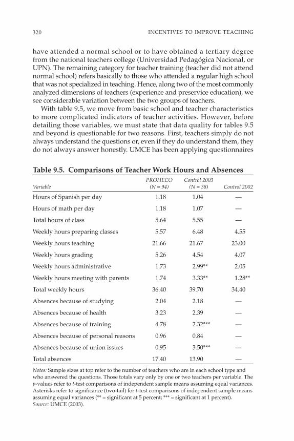
have attended a normal school or to have obtained a tertiary degreefrom the national teachers college (Universidad Pedagógica Nacional, orUPN). The remaining category for teacher training (teacher did not attendnormal school) refers basically to those who attended a regular high schoolthat was not specialized in teaching. Hence, along two of the most commonlyanalyzed dimensions of teachers (experience and preservice education), wesee considerable variation between the two groups of teachers.
With table 9.5, we move from basic school and teacher characteristicsto more complicated indicators of teacher activities. However, beforedetailing those variables, we must state that data quality for tables 9.5and beyond is questionable for two reasons. First, teachers simply do notalways understand the questions or, even if they do understand them, theydo not always answer honestly. UMCE has been applying questionnaires
320 INCENTIVES TO IMPROVE TEACHING
Table 9.5. Comparisons of Teacher Work Hours and AbsencesPROHECO Control 2003
Variable (N = 94) (N = 38) Control 2002
Hours of Spanish per day 1.18 1.04 —
Hours of math per day 1.18 1.07 —
Total hours of class 5.64 5.55 —
Weekly hours preparing classes 5.57 6.48 4.55
Weekly hours teaching 21.66 21.67 23.00
Weekly hours grading 5.26 4.54 4.07
Weekly hours administrative 1.73 2.99** 2.05
Weekly hours meeting with parents 1.74 3.33** 1.28**
Total weekly hours 36.40 39.70 34.40
Absences because of studying 2.04 2.18 —
Absences because of health 3.23 2.39 —
Absences because of training 4.78 2.32*** —
Absences because of personal reasons 0.96 0.84 —
Absences because of union issues 0.95 3.50*** —
Total absences 17.40 13.90 —
Notes: Sample sizes at top refer to the number of teachers who are in each school type andwho answered the questions. Those totals vary only by one or two teachers per variable. Thep-values refer to t-test comparisons of independent sample means assuming equal variances.Asterisks refer to significance (two-tail) for t-test comparisons of independent sample meansassuming equal variances (** = significant at 5 percent; *** = significant at 1 percent).Source: UMCE (2003).

of this kind for almost 10 years, and with each successive data collection,the process is improving. But the reality is that a culture of evaluation doesnot exist in Honduras (or in many places), and teachers may feel the needto tailor their responses to what they think they “should” be saying. Orthey may simply not answer, which will become more apparent as, forsome kinds of questions, more missing cases arise. Again, UMCE hasmade great strides in reducing the quantity of missing answers. Comparedwith most data collection projects, the number of missing student andteacher answers is not large. But if certain kinds of teachers are notanswering the questions, or are falsifying their answers, then those kindsof comparisons will have little validity, hence the difficulty of relying onteacher responses instead of observing actual actions.
A commonly cited justification for empowering parental councils is thatteachers’ effort will increase with greater parental participation. Table 9.5shows mixed results for this rationale. PROHECO teachers report spend-ing more time teaching the basic subjects (math and Spanish), but the dif-ferences are not statistically significant, and their overall reported classtime is identical. The same is true with overall weekly hours; the Control2003 school teachers actually report more time spent in the school (butthe differences are insignificant). However, the individual time categoriesshow some interesting differences. First, Control 2003 school teachersspend almost twice as much time as PROHECO teachers in administrativetasks. So the image of a more “streamlined” delivery in PROHECO findssupport. However, PROHECO teachers report significantly less time eachweek meeting with parents compared with Control 2003 and significantlymore time than Control 2002 teachers. Table 9.2 showed that mothers workmore in the Control 2002 sample, which may, in turn, have affected theirability to meet with teachers.
Do PROHECO teachers work more days? The tentative answer is no, butthe breakdown of teacher absences (available only with the 2003 data)shows some important differences.125 PROHECO teachers appear to missmore days because of training. This finding is perhaps not unexpected,given their comparatively low levels of preservice education. Not surpris-ingly, Control 2003 teachers miss almost four times as many days becauseof meetings with their union. Unfortunately, the most valid comparison ofteacher attendance requires data on unexcused absences that are not likelyto be reported by teachers in these kinds of questions. Unexcused absencesappear to be a severe problem in rural Honduras (Bedi and Marshall 2002),and with a payment schedule based on days worked, it would seem thatPROHECO schools are well equipped to reduce these kinds of absences.
321TEACHER EFFORT AND SCHOOLING OUTCOMES
125. The 2002 teacher questionnaire has data on teachers’ absences, but it uses a differentmeasurement scale so it cannot be compared with the data collected in 2003 for PROHECO.

The fact that the data in table 9.5 imply otherwise should not be taken tooliterally because the absences in table 9.5 are probably restricted to theones the teacher is comfortable reporting. We will return to this issue belowwhen we compare student responses about teacher absences.
An imperfect way of assessing teacher quality and parental valuation ofschool quality is by comparing teachers’ salaries in PROHECO and thecontrol school (in 2003 only). The results in table 9.6 show that Control2003 teachers earn significantly more than PROHECO teachers. This find-ing is not surprising when considering their higher levels of education andexperience, although it should be pointed out that only about half of thecontrol teachers responded to this question. Interestingly, PROHECOteachers report more problems with receiving their pay than do controlteachers. This statistic does cast some doubt on the effectiveness of thePROHECO business model, at least in terms of payment delivery. In bothschool types, teachers report late pay in about half of the cases, but in thePROHECO schools, the delays are much longer.
With multivariate analysis, we can make even more specific com-parisons between PROHECO and Control 2003 teachers’ salaries. Theresults in table 9.7 show that, when controlling experience and education,PROHECO teachers earn about 10 percent less than their counterparts.Again, because less than half of the control school teachers responded, thiscomparison may be meaningless in reality. But the result is intriguing. First,it suggests that PROHECO parents are not necessarily interested in recruit-ing the best teachers available. Or, because of supply-side restrictions(namely, teacher availability), the teachers they do get to work in their com-munities are of lower quality. The difference in quality (as defined bysalary) becomes even greater between PROHECO teachers and control
322 INCENTIVES TO IMPROVE TEACHING
Table 9.6. Comparisons of Teacher Salaries and Payment “Issues”PROHECO Control 2003
Variable (N = 90) (N = 17) Control 2002
Teachers’ salary in school 3,046.10 3,846.60*** —
Teachers’ salary outside school 867.70 1,302.10 —
Salary ever arrived late 0.50 0.53 —
How many days late? 26.60 4.70*** —
Notes: Sample sizes at the top of the table refer to the number of teachers who are in eachschool type and who answered the questions. Those totals vary only by one or two teachersper variable. Unless otherwise noted, all variables are 0–1 where 1 indicates Yes. The p-valuesrefer to t-test comparisons of independent sample means assuming equal variances. Asterisksrefer to significance (two-tail) for t-test comparisons of independent sample means assumingequal variances (*** = significant at 1 percent).Source: UMCE (2003).

teachers if we consider the possibility that those communities are moredifficult places to work. This assumption may not hold, for any number ofreasons.126 However, if it is true, then those communities will, in theory,have to pay more to get the same level of quality.
Making inferences about teacher quality on the basis of salary is purelyspeculative at this point, and more important issues remain. Note thatteacher quality in Honduras is determined more by bureaucratic fiat thanby performance, as demonstrated in table 9.7 by the returns to variableslike experience and education that may in reality have little to say aboutquality. The data analysis of student outcomes will, presumably, shedmore light on teacher quality. Furthermore, by transforming the manage-
323TEACHER EFFORT AND SCHOOLING OUTCOMES
Table 9.7. Teacher Earnings EquationsVariable PROHECO teachers Control 2003 teachers
PROHECO school −0.10 (−1.99)** −0.12 (−2.27)**
Teacher is female 0.01 (0.77) 0.01 (0.53)
Teacher is from area 0.03 (1.55) 0.02 (1.12)
Teachers’ experience (months) 0.001 (3.55)*** 0.001 (3.69)***
Teacher has post in school −0.04 (−0.87) −0.04 (−0.85)
Teacher attended normal school 0.15 (7.14)*** 0.15 (6.34)***
Teacher attended UPN 0.17 (4.76)*** 0.18 (4.61)***
School is single teacher 0.05 (1.98) 0.05 (1.76)*
School is double teacher 0.06 (2.85)*** 0.06 (2.42)***
State fixed effects? No Yes (1.29)
Sample size 96.00 96.00
R2 0.69 0.76
Notes: Dependent variable is natural log of monthly (teacher reported) salary in lempiras. Twoteachers who reported 0 were dropped from this sample. Teacher attended normal school andUPN dummies are interpreted in relation to non-normal and non-UPN teachers. Single anddouble teacher school dummies are interpreted in relation to multidocente schools. Asterisksrefer to significance (two-tail) for t-test comparisons of independent sample means assumingequal variances (* = significant at1 0 percent; ** = significant at 5 percent; *** = significantat 1 percent). Figures shown in parentheses are t-statistics. For the estimation of state fixedeffects, the number in parentheses is the F-test for significance of state effects (p = 0.23).Source: UMCE (2003).
126. Very likely, the PROHECO communities are, on average, more isolated than tradi-tional school locations. But teachers may see those jobs as more attractive along other dimen-sions such as nonpecuniary remuneration (meals and so forth) or safer living arrangements.

ment process, the PROHECO schools may be more efficient, which wouldresult in equal learning for less money. This outcome, of course, echoesFriedman’s original argument for school choice in which he found the result-ing system will be cheaper if not necessarily better. PROHECO parents maynot be looking to build the best schools in Honduras; they may simply wantthe most efficient schools. Finally, these data say nothing about class size.Because PROHECO schools are keeping the student–teacher ratio low (seetable 9.3), one could argue that the overall workload for teachers is lower andthat less quality is needed overall. In other words, the total per pupil expen-diture on quality may be more equal than what is implied by the results.
One of the most challenging aspects of comparing teachers concernsthe methodologies they use in the classroom. Observational data on teach-ing processes are time-consuming data to collect and are very difficult towork into multivariate analysis (for example, see Marshall 2003). Soinstead, most researchers ask teachers to describe their methods. UMCEefforts have achieved some success using student responses about teachingstrategies (UMCE, UPN, and SE 2003), and these data are also incorporatedhere (see table 9.8). Table 9.8 begins this line of analysis by comparingteacher responses about teaching methods from PROHECO and Control2003 samples. The results reveal few significant differences. PROHECOteachers indicate that they use circles rather than groups (or rows) more fre-quently than control teachers, but the importance of this result is not clear.As for teaching strategies (for example, the frequency they have studentsworking in pairs, by themselves, with worksheets, and so forth), no signif-icant differences were found between the two groups of teachers.
Table 9.9 also reveals few differences in teaching processes betweenPROHECO and control samples. In general, teachers base their plans onthe textbooks and the learning objectives. The only significant difference isfor real-life situations, where the control group teachers indicate they aremore likely to use examples from real life in their planning. The remainingvariables are nearly identical for both groups.
In table 9.10, we continue the comparisons of teaching behaviors, asreported by teachers. In the first exercise, each teacher was asked to rankfrom 1 (most frequent) to 7 (least frequent) the methods they most fre-quently use in the classroom. Therefore, the lower the mean, the morefrequently teachers use the strategy. The results show that PROHECOteachers report more dictation (p-value = 0.15), give fewer examples, andare less likely to use a learning dynamic (definition is uncertain). Thosedata are hardly sufficient for making sweeping conclusions about class-room processes. But they do not paint a picture of more active teachingstrategies. Previous UMCE data have shown that teachers who use moredictation appear to be less effective. PROHECO teachers also continue toreport less interaction with parents, although this difference is statisti-cally insignificant. In addition, they do not report giving more homework.
324 INCENTIVES TO IMPROVE TEACHING

The only other differences in means that approach statistical significanceare for the frequency with which teachers let students grade homework(more in PROHECO) and the frequency with which teachers use shortanswer tests (more in PROHECO).
How do PROHECO teachers compare with control school teachers interms of their evaluation of the work environment? Table 9.11 presentsdata about teacher opinions, although it should be noted once again thata large group (about 20) of Control 2003 teachers did not respond. If thosewho did not respond chose not to participate because they are generallyunhappy with teaching, then the comparisons have no meaning. Theresults once again reveal few significant differences. It is interesting thatPROHECO teachers report getting along better with parents (the defini-tion of this question is not exact), which would appear to contradict theearlier data indicating less frequent contact. However, the two things arenot necessarily the same. The only significant difference is related to pay;
325TEACHER EFFORT AND SCHOOLING OUTCOMES
Table 9.8. Comparisons of Teaching StrategiesPROHECO Control 2003
Variable (N = 94) (N = 38) Control 2002
Does the teacher—
Organize students in rows? 0.11 0.11 —
Organize students in circle? 0.18 0.00*** —
Organize students in groups? 0.71 0.89** —
Frequency teacher has students—
Work alone 0.81 0.94 —
Work alone with help from teacher 1.53 1.44 —
Listen to teacher 1.66 1.64 —
Work in pairs 0.88 1.06 —
Work in pairs with help from teacher 1.66 1.60 —
Work with worksheets 0.96 1.06 —
Have contests 1.17 1.35 —
Notes: Sample sizes at the top of the table refer to the number of teachers who are in eachschool type and who answered the questions. Those totals vary only by one or two teachersper variable. The p-values refer to t-test comparisons of independent sample means assumingequal variances. For frequency, the options are coded 0 (Never), 1 (Sometimes), 2 (Always).Asterisks refer to significance (two-tail) for t-test comparisons of independent sample meansassuming equal variances (** = significant at 5 percent; *** = significant at 1 percent).Source: UMCE (2003).
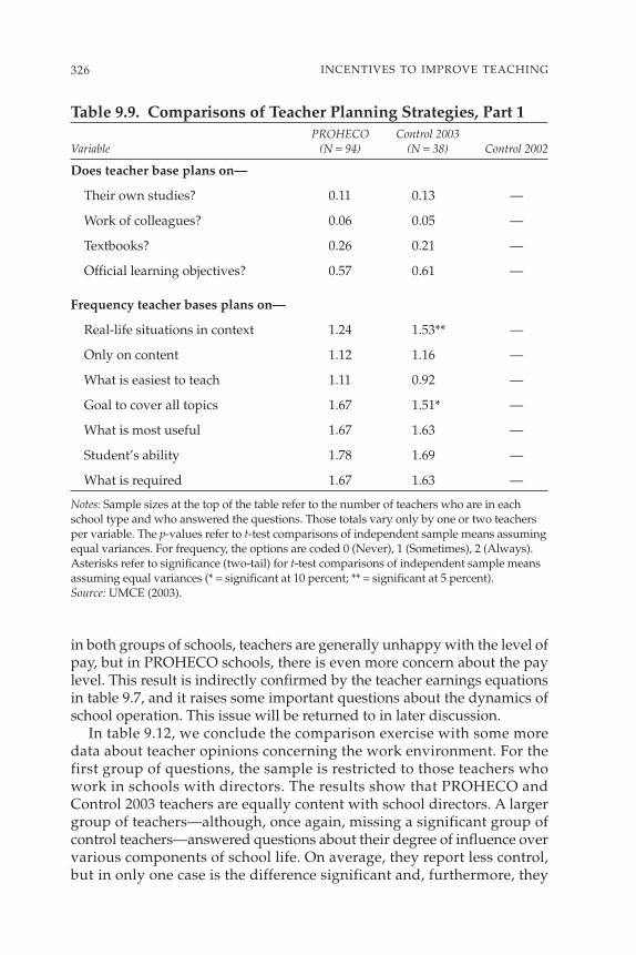
in both groups of schools, teachers are generally unhappy with the level ofpay, but in PROHECO schools, there is even more concern about the paylevel. This result is indirectly confirmed by the teacher earnings equationsin table 9.7, and it raises some important questions about the dynamics ofschool operation. This issue will be returned to in later discussion.
In table 9.12, we conclude the comparison exercise with some moredata about teacher opinions concerning the work environment. For thefirst group of questions, the sample is restricted to those teachers whowork in schools with directors. The results show that PROHECO andControl 2003 teachers are equally content with school directors. A largergroup of teachers—although, once again, missing a significant group ofcontrol teachers—answered questions about their degree of influence overvarious components of school life. On average, they report less control,but in only one case is the difference significant and, furthermore, they
326 INCENTIVES TO IMPROVE TEACHING
Table 9.9. Comparisons of Teacher Planning Strategies, Part 1PROHECO Control 2003
Variable (N = 94) (N = 38) Control 2002
Does teacher base plans on—
Their own studies? 0.11 0.13 —
Work of colleagues? 0.06 0.05 —
Textbooks? 0.26 0.21 —
Official learning objectives? 0.57 0.61 —
Frequency teacher bases plans on—
Real-life situations in context 1.24 1.53** —
Only on content 1.12 1.16 —
What is easiest to teach 1.11 0.92 —
Goal to cover all topics 1.67 1.51* —
What is most useful 1.67 1.63 —
Student’s ability 1.78 1.69 —
What is required 1.67 1.63 —
Notes: Sample sizes at the top of the table refer to the number of teachers who are in eachschool type and who answered the questions. Those totals vary only by one or two teachersper variable. The p-values refer to t-test comparisons of independent sample means assumingequal variances. For frequency, the options are coded 0 (Never), 1 (Sometimes), 2 (Always).Asterisks refer to significance (two-tail) for t-test comparisons of independent sample meansassuming equal variances (* = significant at 10 percent; ** = significant at 5 percent).Source: UMCE (2003).

327TEACHER EFFORT AND SCHOOLING OUTCOMES
Table 9.10. Comparisons of Teaching Strategies, Part 2PROHECO Control 2003
Variable (N = 83) (N = 35) Control 2002
Frequency (1 = most, 7 = least) with which the teacher
Dictates to class 3.94 4.63 —
Reviews with class 3.63 3.74 —
Gives examples 4.11 3.31** —
Uses chalkboard 4.20 4.22 —
Uses learning dynamic 4.14 3.19** —
Uses exercises 4.64 4.44 —
Uses questions 4.73 4.44 —
Frequency of parent meetings 2.49 2.67 —
Frequency with which teacher gives homework 2.75 2.68 —
Frequency (0 never, 1 = sometimes, 2 = always) with which the teacher
Records homework 1.97 2.00 —
Grades homework 1.58 1.58 —
Reviews homework 1.71 1.78 —
Lets students grade homework 1.46 1.29 —
Focuses on errors from homework 1.66 1.58 —
Uses homework in grading 1.56 1.67 —
Frequency with which teacher bases evaluation on
Standardized tests 0.54 0.57 —
Short answer tests 1.60 1.43* —
Classroom observations 1.90 1.84 —
Classroom questions 1.76 1.76 —
Homework 1.54 1.78* —
Multiple-choice tests 1.68 1.73 —
Notes: Sample sizes at the top of the table refer to the number of teachers who are in eachschool type and who answered the questions. Those totals vary only by one or two teachersper variable. The p-values refer to t-test comparisons of independent sample means assum-ing equal variances. For frequency, the teachers were asked to rank the seven options from1 (most frequent) to 7 (least frequent), so higher values mean this strategy is less frequentlyincorporated in the classroom. Asterisks refer to significance (two-tail) for t-test comparisonsof independent sample means assuming equal variances (* = significant at 10 percent; ** = significant at 5 percent).Source: UMCE (2003).
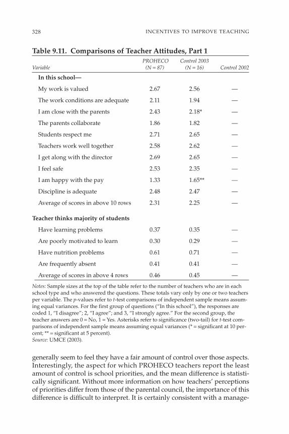
generally seem to feel they have a fair amount of control over those aspects.Interestingly, the aspect for which PROHECO teachers report the leastamount of control is school priorities, and the mean difference is statisti-cally significant. Without more information on how teachers’ perceptionsof priorities differ from those of the parental council, the importance of thisdifference is difficult to interpret. It is certainly consistent with a manage-
328 INCENTIVES TO IMPROVE TEACHING
Table 9.11. Comparisons of Teacher Attitudes, Part 1PROHECO Control 2003
Variable (N = 87) (N = 16) Control 2002
In this school—
My work is valued 2.67 2.56 —
The work conditions are adequate 2.11 1.94 —
I am close with the parents 2.43 2.18* —
The parents collaborate 1.86 1.82 —
Students respect me 2.71 2.65 —
Teachers work well together 2.58 2.62 —
I get along with the director 2.69 2.65 —
I feel safe 2.53 2.35 —
I am happy with the pay 1.33 1.65** —
Discipline is adequate 2.48 2.47 —
Average of scores in above 10 rows 2.31 2.25 —
Teacher thinks majority of students
Have learning problems 0.37 0.35 —
Are poorly motivated to learn 0.30 0.29 —
Have nutrition problems 0.61 0.71 —
Are frequently absent 0.41 0.41 —
Average of scores in above 4 rows 0.46 0.45 —
Notes: Sample sizes at the top of the table refer to the number of teachers who are in eachschool type and who answered the questions. These totals vary only by one or two teachersper variable. The p-values refer to t-test comparisons of independent sample means assum-ing equal variances. For the first group of questions (“In this school”), the responses arecoded 1, “I disagree”; 2, “I agree”; and 3, “I strongly agree.” For the second group, theteacher answers are 0 = No, 1 = Yes. Asterisks refer to significance (two-tail) for t-test com-parisons of independent sample means assuming equal variances (* = significant at 10 per-cent; ** = significant at 5 percent).Source: UMCE (2003).

ment framework where parents are empowered. But knowing more aboutthe kinds of priorities that teachers think are important would be inter-esting, especially in terms of how they differ from what priorities parentsthink are important.
For most of the comparisons made in this section, we have relied onthe teacher questionnaire. However, as mentioned before, there are somereasons to be suspicious about the validity of teacher responses. Anotherway of getting at teaching and learning environments is by aggregating
329TEACHER EFFORT AND SCHOOLING OUTCOMES
Table 9.12. Comparisons of Teacher Attitudes, Part 2PROHECO Control 2003
Variable (N = 43) (N = 11) Control 2002
Teacher appraisal (1 = inefficient, 4 = very good) of school director’s management of
Materials 3.19 2.82 —
Teacher training 2.51 2.64 —
Coordination 3.14 3.00 —
Organization of school 2.86 2.80 —
Conflicts 3.02 3.00 —
Commissions 3.32 3.45 —
Average of scores in above 6 rows 2.99 2.98 —
Teacher assessment (1 = little, 2 = some, 3 = a lot) of control over
Teaching methodology 2.64 2.82 —
Use of materials 2.41 2.59 —
School priorities 2.19 2.59** —
Decisions 2.72 2.66 —
Rules 2.64 2.76 —
Planning 2.64 2.71 —
Average of scores in above 6 rows 2.54 2.66 —
Would you leave teaching if giventhe opportunity? 0.15 0.22 —
Notes: Sample sizes at the top of the table refer to the number of teachers who are in eachschool type and who answered the questions. Those totals vary only by one or two teachersper variable. The p-values refer to t-test comparisons of independent sample means assumingequal variances. Asterisks refer to significance (two-tail) for t-test comparisons of independentsample means assuming equal variances (** = significant at 5 percent).Source: UMCE (2003).

student responses concerning some of these dimensions. Table 9.13 presentsthe results of comparisons among the three types of schools (when possible),using several questions that appear on the student interview. The resultsreveal some interesting differences. First, according to students, Control2003 teachers were more frequently absent in 2003 than the PROHECOteachers. Results also seem to indicate that PROHECO teachers make moreuse of dictation and chalkboard examples when teaching. Student responsescorroborate the teachers and show that Control 2003 school teachers makemore use of homework, but given the differences in socioeconomic sta-tus between Control 2003 and PROHECO, this finding may simply reflectstudents’ ability to do homework rather than teachers’ effort. Control 2003students also report more physical problems with classrooms and schoolenvironments than do students in PROHECO schools, which is consistentwith previous comparisons. However, a surprising finding is that the Con-trol 2002 students actually report fewer problems. Finally, for 2003, we see
330 INCENTIVES TO IMPROVE TEACHING
Table 9.13. Comparisons of School Environments According to StudentsVariable PROHECO Control 2003 Control 2002
How frequently is the teacher absent? 1.54 1.94*** —
Predominant teaching methodology:
Dictation 0.23 0.20** 0.19**
Teacher works at chalkboard 0.44 0.37*** 0.41
Students work in groups 0.10 0.15*** 0.14***
Question and answer 0.07 0.09 0.25***
Other 0.17 0.20 0.01
Frequency of homework:
In Spanish 3.38 3.47** —
In mathematics 3.50 3.58** —
Number of problems in classroom 0.93 1.14*** 0.80***
Frequency of fights with students 0.16 0.31*** —
Notes: Sample sizes at the top of the table refer to the number of teachers who are in eachschool type and who answered the questions. Those totals vary only by one or two teachersper variable. The p-values refer to t-test comparisons of independent sample means assumingequal variances. For frequency, the options are coded 0 (Never), 1 (Sometimes), 2 (Always).Asterisks refer to significance (two-tail) for t-test comparisons of independent sample meansassuming equal variances (** = significant at 5 percent; *** = significant at 1 percent).Source: UMCE, 2003.
that PROHECO school environments are less chaotic; PROHECO studentsreport fewer fights with other students. Previous work in Central America(Marshall 2003) has identified student violence as a significant predictor ofgrade attainment and has found that PRONADE schools in Guatemalahad less violence among students. The result in table 9.13 suggests that onemechanism that may link community schooling with better student out-comes is an increased awareness of how students are getting along.
First-Order Effects: Teacher and School Effort
The previous section showed little evidence that teacher effort in PROHECOschools is greater than in the control schools. But this data point is a verydifficult one to measure, so we should be wary of making sweeping con-clusions. Furthermore, given the differences between treatment and con-trol in this sample, we also cannot rule out the possibility that realdifferences exist. In this section, we continue this discussion, first withadditional simple comparisons using the Director questionnaire and thenin a more demanding framework using multivariate analysis.
Table 9.14 concludes the comparisons of means analysis with the direc-tor responses. Once again, we have the problem of “equalizing” the databetween two years, and the result is that, for 2002, only some of the dataare available. Table 9.14 shows some interesting differences. Not surpris-ingly, directors in control schools are more likely to have universitydegrees, and the control schools receive more frequent visits from districtsupervisors. Not many differences are apparent in directors’ use of time.
Another unsurprising finding is that PROHECO schools are closed lessfrequently for work stoppages than control schools, although the averagesare about even for the remaining categories. Work stoppages can occurbecause of lack of teachers, teachers’ absences, teachers’ strikes, and soforth. Our evidence shows that fewer work stoppages occur in PROHECOschools, that work stoppages do not translate into school closings, or both.Fewer work stoppages may be attributed to the fact that teachers are hireddirectly by the school, that they are hired according to yearly renewablecontracts (with, therefore, the threat not to be rehired), and that commu-nities are involved in the monitoring of the school. Fewer school closingsafter work stoppages may be attributed to community “activeness” thatmakes sure an absent teacher is replaced. In any case, PROHECO schoolsgain some work days.
PROHECO directors report significantly less autonomy than Control2002 directors. This finding is an interesting one, but it is not inconsistentwith what teachers indicated earlier. In PROHECO schools, the parentshave more responsibility (in theory), and this dynamic appears to retardthe degree of autonomy felt by school personnel.
331TEACHER EFFORT AND SCHOOLING OUTCOMES

Finally, a particularly surprising finding is that Control 2003 schoolsreport more frequent parent meetings. Some caution is urged here, how-ever, because a large group (about 20) of control schools reported no datafor this question. So we cannot rule out the possibility that the only oneswho reported are the ones with the most active parent associations. An
332 INCENTIVES TO IMPROVE TEACHING
Table 9.14. School Characteristics According to DirectorsVariable PROHECO Control 2003 Control 2002
Director has a university degree 0.06 0.28*** 0.08
Frequency district supervisor visits 1.16 1.71** 1.71**
Percentage of time director spends
Administrating issues 10.9 9.9 16.1***
Organizing activities 15.7 12.8* 18.7
Meeting with community 5.1 5.5 9.6**
Meeting with teachers 9.2 8.7 10.2
Meeting with parents 13.4 11.2 12.8
Teaching 41.7 44.7 43.5
Number of school closings because of
Holidays 6.1 6.9 —
Bureaucratic processes 2.2 2.3 —
Work stoppages 0.4 6.2*** —
Union meetings 2.1 3.2 —
Training sessions 4.5 4.1 —
Parties 0.6 0.7 —
SEP 0.7 2.0*** —
Total closings 20.5 29.5*** —
Average director autonomy 1.3 1.2 1.7***
Average parental capacity and involvement 1.7 1.7 —
Frequency of parent meetings 1.7 2.6*** —
Notes: The p-values refer to t-test comparisons of independent sample means assumingequal variances. Asterisks refer to significance (two-tail) for t-test comparisons of indepen-dent sample means assuming equal variances (* = significant at 10 percent; ** = significantat 5 percent; *** = significant at 1 percent).Source: UMCE (2003).

additional problem—already referred to with teachers—is definitional.PROHECO directors may not consider the PROHECO parent associa-tions to be associations per se; they may use a different terminology thanthat used in the public system. It seems hard to believe that parents inPROHECO schools have fewer meetings. Nevertheless, this issue hasalready been raised earlier, and we cannot discard the possibility thatPROHECO schools are run by parent councils that are not necessarilymore involved in day-to-day operations than control school parents.
We now turn to the multivariate analysis of teacher and school effort.This analysis is an important component of this study, because we expectthe mechanism linking PROHECO with improved student outcomes tobe a more efficient workplace environment. In other words, existing capac-ity should be better maximized in PROHECO schools. Unfortunately, theresults from these analyses (presented in table 9.15) reveal little in theway of a significant systematic relationship between PROHECO partici-pation and outcomes of teacher and school effort. Caution is urged whendrawing conclusions from those estimations, however, because of the mea-surement problems with most of the dependent variables and the smallsample sizes.
The results in table 9.15 include a total of 11 different outcomes chosenfrom the student, teacher, and director questionnaires. The only parameterthat is presented is for the PROHECO dummy. Interested readers canobtain the full results on request, but the reality is that very few variablesof any kind are significant predictors of those outcomes. For example,the independent variable for frequency of parental meetings (according tothe director) is never a significant predictor of any of the dependent vari-ables for teacher or school effort. The only indicator of accountabilitythat approaches significance in at least some of the estimations is the vari-able for the frequency of district supervisor visits. So given the insignifi-cance of the other predictors and the quantity of outcomes considered(13 dependent variables with three models), those other variables areexcluded from table 9.15.
All data are taken from the 2003 data collection, and each of the depen-dent variables is detailed in the previous section when we comparedmeans. Three models are estimated for each outcome. The first includesonly the PROHECO dummy and basic teacher (when it is a teacher-specificoutcome) and school characteristics such as experience, gender, and schooltype (single teacher, and so forth). In the second model, we add additionalschool characteristics such as the frequency of district supervisor visits,parental meetings (when the outcome is not parental meetings), and schoolsize. Finally, in model 3, the department dummies and socioeconomiccontrols are added. All estimations are done at the school or teacher level,which involves sample sizes of between 95 and 130. Those are very smallsamples from which to obtain efficient and robust parameters.
333TEACHER EFFORT AND SCHOOLING OUTCOMES
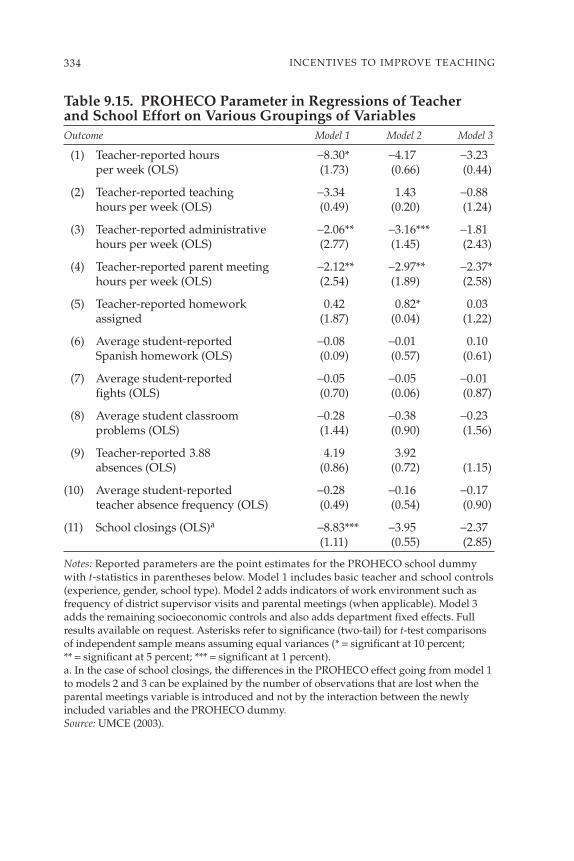
334 INCENTIVES TO IMPROVE TEACHING
Table 9.15. PROHECO Parameter in Regressions of Teacher and School Effort on Various Groupings of VariablesOutcome Model 1 Model 2 Model 3
(1) Teacher-reported hours −8.30* −4.17 −3.23 per week (OLS) (1.73) (0.66) (0.44)
(2) Teacher-reported teaching −3.34 1.43 −0.88 hours per week (OLS) (0.49) (0.20) (1.24)
(3) Teacher-reported administrative −2.06** −3.16*** −1.81 hours per week (OLS) (2.77) (1.45) (2.43)
(4) Teacher-reported parent meeting −2.12** −2.97** −2.37* hours per week (OLS) (2.54) (1.89) (2.58)
(5) Teacher-reported homework 0.42 0.82* 0.03 assigned (1.87) (0.04) (1.22)
(6) Average student-reported −0.08 −0.01 0.10 Spanish homework (OLS) (0.09) (0.57) (0.61)
(7) Average student-reported −0.05 −0.05 −0.01 fights (OLS) (0.70) (0.06) (0.87)
(8) Average student classroom −0.28 −0.38 −0.23 problems (OLS) (1.44) (0.90) (1.56)
(9) Teacher-reported 3.88 4.19 3.92 absences (OLS) (0.86) (0.72) (1.15)
(10) Average student-reported −0.28 −0.16 −0.17 teacher absence frequency (OLS) (0.49) (0.54) (0.90)
(11) School closings (OLS)a −8.83*** −3.95 −2.37 (1.11) (0.55) (2.85)
Notes: Reported parameters are the point estimates for the PROHECO school dummywith t-statistics in parentheses below. Model 1 includes basic teacher and school controls(experience, gender, school type). Model 2 adds indicators of work environment such asfrequency of district supervisor visits and parental meetings (when applicable). Model 3adds the remaining socioeconomic controls and also adds department fixed effects. Fullresults available on request. Asterisks refer to significance (two-tail) for t-test comparisonsof independent sample means assuming equal variances (* = significant at 10 percent; ** = significant at 5 percent; *** = significant at 1 percent).a. In the case of school closings, the differences in the PROHECO effect going from model 1to models 2 and 3 can be explained by the number of observations that are lost when theparental meetings variable is introduced and not by the interaction between the newlyincluded variables and the PROHECO dummy.Source: UMCE (2003).

As mentioned earlier, table 9.15 provides little in the way of systematicevidence to link PROHECO participation with increased teacher effort,although some evidence indicates a positive PROHECO effect. Worthmentioning is that those dependent variables are very difficult to measure.The significant parameters are in both directions. For example, PROHECOteachers report fewer hours of work per week. Not surprisingly, they reportsignificantly fewer hours per week in administrative duties. But they alsoreport significantly less time devoted to meetings with parents. This issue hasalready been addressed, and it seems surprising that PROHECO teachershave less interaction with parents. One explanation may be that, instead,PROHECO teachers interpret the term parent meeting differently. Never-theless, this issue is an open question that deserves more attention in thefuture. On the positive side, PROHECO students report fewer problems inthe classroom than non-PROHECO students, although the point estimatesonly approach statistical significance. Additionally, PROHECO teachersreport more homework, with point estimates that reach significance inmodel 2. Finally, evidence confirms that the PROHECO schools are asso-ciated with fewer closings according to the director.
Taken together, the results in table 9.15 highlight the importance ofcollecting more and better data on first-order, procedural outcomes inHonduran schools. This emphasis is not to say that the UMCE data areinappropriate for evaluating the effect of PROHECO. But the real chal-lenge in identifying the effect of a program like PROHECO lies in explain-ing differences in classroom and school environments because those are, intheory, the mechanisms that link increased parental participation withimprovements in student outcomes.
Second-Order Effects: Academic Achievement and Student Flows
We review below second-order effects of PROHECO schools. In the firsttwo subsections, we provide an analysis of academic achievement levelsand variance decomposition. In the third subsection, we analyze academicachievement while controlling for selection bias. Finally, we analyze theeffect of PROHECO schools on student flows.
Academic AchievementIf PROHECO schools have succeeded in transforming the teaching andlearning environment, then we should expect second-order—or indirect—effects to turn up in student outcomes. Test scores are the most commonlyused measure of school production, in addition to pass rates and desertion.With multivariate analysis, as detailed in the methodology section, we canbegin to form a causal argument relating PROHECO participation withstudent outcomes. The previous section relied largely on simple t-tests, but
335TEACHER EFFORT AND SCHOOLING OUTCOMES
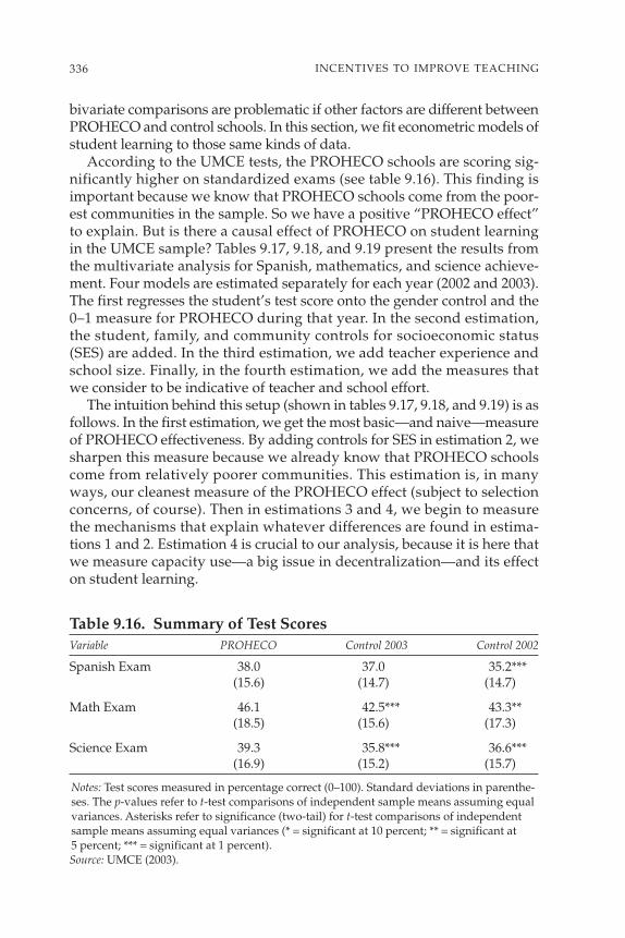
bivariate comparisons are problematic if other factors are different betweenPROHECO and control schools. In this section, we fit econometric models ofstudent learning to those same kinds of data.
According to the UMCE tests, the PROHECO schools are scoring sig-nificantly higher on standardized exams (see table 9.16). This finding isimportant because we know that PROHECO schools come from the poor-est communities in the sample. So we have a positive “PROHECO effect”to explain. But is there a causal effect of PROHECO on student learningin the UMCE sample? Tables 9.17, 9.18, and 9.19 present the results fromthe multivariate analysis for Spanish, mathematics, and science achieve-ment. Four models are estimated separately for each year (2002 and 2003).The first regresses the student’s test score onto the gender control and the0–1 measure for PROHECO during that year. In the second estimation,the student, family, and community controls for socioeconomic status(SES) are added. In the third estimation, we add teacher experience andschool size. Finally, in the fourth estimation, we add the measures thatwe consider to be indicative of teacher and school effort.
The intuition behind this setup (shown in tables 9.17, 9.18, and 9.19) is asfollows. In the first estimation, we get the most basic—and naive—measureof PROHECO effectiveness. By adding controls for SES in estimation 2, wesharpen this measure because we already know that PROHECO schoolscome from relatively poorer communities. This estimation is, in manyways, our cleanest measure of the PROHECO effect (subject to selectionconcerns, of course). Then in estimations 3 and 4, we begin to measurethe mechanisms that explain whatever differences are found in estima-tions 1 and 2. Estimation 4 is crucial to our analysis, because it is here thatwe measure capacity use—a big issue in decentralization—and its effecton student learning.
336 INCENTIVES TO IMPROVE TEACHING
Table 9.16. Summary of Test ScoresVariable PROHECO Control 2003 Control 2002
Spanish Exam 38.0 37.0 35.2*** (15.6) (14.7) (14.7)
Math Exam 46.1 42.5*** 43.3** (18.5) (15.6) (17.3)
Science Exam 39.3 35.8*** 36.6*** (16.9) (15.2) (15.7)
Notes: Test scores measured in percentage correct (0–100). Standard deviations in parenthe-ses. The p-values refer to t-test comparisons of independent sample means assuming equalvariances. Asterisks refer to significance (two-tail) for t-test comparisons of independentsample means assuming equal variances (* = significant at 10 percent; ** = significant at 5 percent; *** = significant at 1 percent).Source: UMCE (2003).
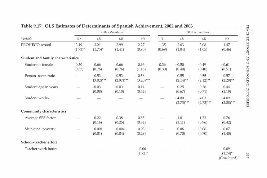
337T
EA
CH
ER
EF
FO
RT
AN
DSC
HO
OL
ING
OU
TC
OM
ES
Table 9.17. OLS Estimates of Determinants of Spanish Achievement, 2002 and 20032002 estimations 2003 estimations
Variable (1) (2) (3) (4) (1) (2) (3) (4)
PROHECO school 3.19 3.21 2.99 2.27 1.35 2.63 3.08 1.47(1.73)* (1.75)* (1.41) (0.90) (0.69) (1.04) (1.05) (0.46)
Student and family characteristics
Student is female 0.50 0.66 0.66 0.96 0.36 −0.50 −0.49 −0.61(0.57) (0.76) (0.76) (1.16) (0.30) (0.40) (0.40) (0.51)
Person–room ratio — −0.53 −0.53 −0.56 — −0.55 −0.55 −0.57(3.02)*** (2.97)*** (3.20)*** (2.14)** (2.12)** (2.29)**
Student age in years — −0.03 −0.03 0.14 — 0.25 0.26 0.44(0.08) (0.10) (0.42) (0.67) (0.71) (1.19)
Student works — — — — — −4.00 −4.03 −4.09(2.73)*** (2.73)*** (2.88)***
Community characteristics
Average SES factor — 0.22 0.38 −0.55 — 1.81 1.72 0.76(0.16) (0.25) (0.32) (1.11) (0.96) (0.42)
Municipal poverty — −0.001 −0.004 0.03 — −0.06 −0.06 −0.07(0.01) (0.04) (0.29) (0.70) (0.70) (1.40)
School–teacher effort
Teacher work hours — — — 0.06 — — — 0.09(1.72)* (1.74)*
(Continued)

338IN
CE
NT
IVE
ST
OIM
PR
OV
ET
EA
CH
ING
Table 9.17. OLS Estimates of Determinants of Spanish Achievement, 2002 and 2003 (Continued)2002 estimations 2003 estimations
Variable (1) (2) (3) (4) (1) (2) (3) (4)
Average class size — — — −0.12 — — — −0.11(0.77) (1.07)
Frequency of homework — — — — — — — 4.82(1.69)*
School closings — — — — — — — −0.01(0.12)
Remaining controls
Teacher experience — — −0.02 0.01 — — 0.06 0.06(0.13) (0.06) (0.22) (0.23)
Total enrollment — — −0.003 −0.002 — — 0.01 0.02(0.27) (0.17) (0.40) (0.27)
PROHECO dummy — — — — 1.07 — 2.88 0.54after removing (0.56) (1.04) (0.17)outliersa [1] [0] [7] [37]
Fixed effects p-value 0.000 0.000 0.000 0.000 0.000 0.000 0.000 0.000
Sample size 1,257 1,257 1,257 1,257 975 975 975 975
R2 0.050 0.058 0.058 0.073 0.097 0.125 0.125 0.153
Notes: Asymptotic t-statistics in parentheses are based on robust standard errors. All estimations use fixed effects at department level. Asterisks referto significance (two-tail) for t-test comparisons of independent sample means assuming equal variances (* = significant 10 percent; ** = significant at5 percent; *** = significant at 1 percent).a. Parameter for the PROHECO dummy together with the t-statistic and number of dropped cases (in brackets).Source: UMCE (2003).

339T
EA
CH
ER
EF
FO
RT
AN
DSC
HO
OL
ING
OU
TC
OM
ES
Table 9.18. OLS Estimates of Determinants of Mathematics Achievement, 2002 and 20032002 estimations 2003 estimations
Variable (1) (2) (3) (4) (1) (2) (3) (4)
PROHECO school 2.88 4.03 4.62 4.05 2.66 3.80 6.06 5.73 (1.35) (2.67)*** (1.79)* (1.48) (1.17) (1.50) (1.84)* (1.57)
Student and family characteristics
Student is female 0.12 0.28 0.22 0.48 −0.21 −0.75 −0.75 −0.74 (0.13) (0.29) (0.23) (0.51) (0.18) (0.63) (0.64) (0.64)
Person–room ratio — −0.69 −0.73 −0.77 — −0.51 −0.49 −0.58 (3.34)*** (3.51)*** (3.79)*** (2.16)** (2.09)** (2.46)**
Student age in years — −0.08 −0.03 0.12 — −0.01 0.04 0.19 (0.23) (0.08) (0.32) (0.01) (0.10) (0.42)
Student works — — — — — −2.40 −2.56 −2.72 (1.54) (1.63)* (1.85)*
Community characteristics
Average SES factor — 4.03 2.80 1.89 — 2.33 1.81 0.89(2.67)*** (1.53) (0.98) (1.48) (1.14) (0.55)
Municipal poverty — −0.34 −0.32 −0.29 — −0.36 −0.36 −0.33 (2.56)*** (2.41)** (2.13)** (2.74)*** (2.77)*** (2.64)***
School–teacher effort
Teacher work hours — — — 0.07 — — — 0.10(1.47) (1.64)*
(Continued)

340IN
CE
NT
IVE
ST
OIM
PR
OV
ET
EA
CH
ING
Average class size — — — −0.10 — — — 0.02 (0.95) (0.11)
Frequency of homework — — — — — — — 6.05(1.92)*
School closings — — — — — — — 0.01(0.11)
Remaining controls
Teacher experience — — 0.33 0.36 — — 0.28 0.31 (1.31) (1.49) (1.68)* (1.86)*
Total enrollment — — 0.01 0.01 — — 0.01 0.02 (0.87) (0.94) (0.55) (1.07)
PROHECO dummy — — — — 1.49 2.98 7.42 5.08after removing (0.52) (1.14) (2.27)** (1.37)outliersa [1] [1] [7] [34]
Fixed effects p-value 0.000 0.000 0.000 0.000 0.000 0.000 0.000 0.000
Sample size 1,253 1,253 1,253 1,253 952 952 952 952
R2 0.083 0.131 0.140 0.150 0.159 0.198 0.205 0.234
Notes: Asymptotic t-statistics in parentheses are based on robust standard errors. All estimations use fixed effects at department level. Asterisks referto significance (two-tail) for t-test comparisons of independent sample means assuming equal variances (* = significant at 10 percent; ** = significantat 5 percent; *** = significant at 1 percent).a. Parameter for the PROHECO dummy together with the t-statistic and number of dropped cases (in brackets).Source: UMCE (2003).
Table 9.18. OLS Estimates of Determinants of Mathematics Achievement, 2002 and 2003 (Continued)2002 estimations 2003 estimations
Variable (1) (2) (3) (4) (1) (2) (3) (4)

341T
EA
CH
ER
EF
FO
RT
AN
DSC
HO
OL
ING
OU
TC
OM
ES
Table 9.19. OLS Estimates of Determinants of Science Achievement, 2002 and 20032002 estimations 2003 estimations
Variable (1) (2) (3) (4) (1) (2) (3) (4)
PROHECO school 2.33 2.00 2.16 1.00 4.64 5.74 6.99 2.35 (1.22) (1.06) (0.94) (0.41) (2.31)** (2.45)*** (2.32)** (0.76)
Student and family characteristics
Student is female 0.87 1.09 1.03 1.42 −0.10 −0.63 −0.62 −0.86 (0.86) (1.10) (1.05) (1.46) (0.09) (0.54) (0.54) (0.77)
Person–room ratio — −0.58 −0.60 −0.65 — −0.60 −0.60 −0.56 (2.95)*** (3.02)*** (3.30)*** (2.47)*** (2.46)** (2.28)***
Student age in years — 0.35 0.34 0.59 — 0.40 0.43 0.56 (0.89) (0.89) (1.59) (1.02) (1.44) (1.50)
Student works — — — — — −2.52 −2.60 −3.06 (1.76)* (1.83)* (2.23)**
Community characteristics
Average SES factor — 0.96 1.15 −0.19 — 1.68 1.41 0.41 (0.62) (0.69) (0.11) (1.23) (1.06) (0.28)
Municipal poverty — −0.11 −0.12 −0.07 — −0.16 −0.16 −0.14 (1.16) (1.26) (0.78) (1.78)* (1.79)* (1.60)
School–teacher effort
Teacher work hours — — — 0.07 — — — 0.09 (1.95)** (1.80)*
(Continued)
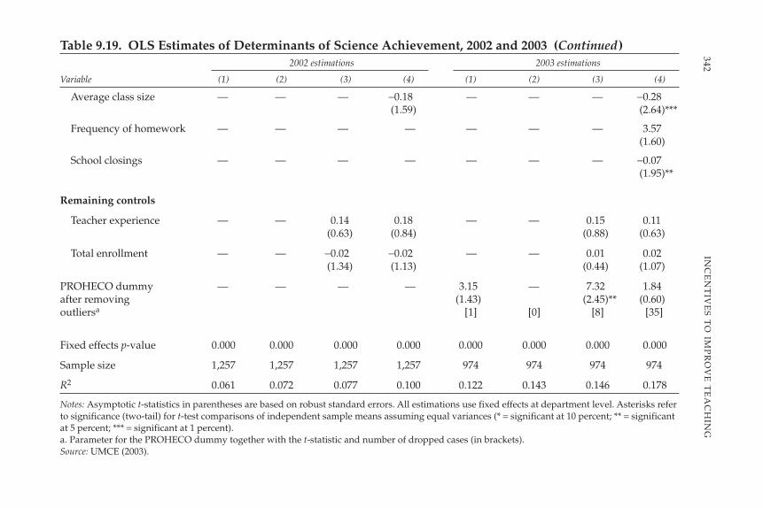
342IN
CE
NT
IVE
ST
OIM
PR
OV
ET
EA
CH
ING
Table 9.19. OLS Estimates of Determinants of Science Achievement, 2002 and 2003 (Continued)2002 estimations 2003 estimations
Variable (1) (2) (3) (4) (1) (2) (3) (4)
Average class size — — — −0.18 — — — −0.28 (1.59) (2.64)***
Frequency of homework — — — — — — — 3.57 (1.60)
School closings — — — — — — — −0.07 (1.95)**
Remaining controls
Teacher experience — — 0.14 0.18 — — 0.15 0.11 (0.63) (0.84) (0.88) (0.63)
Total enrollment — — −0.02 −0.02 — — 0.01 0.02 (1.34) (1.13) (0.44) (1.07)
PROHECO dummy — — — — 3.15 — 7.32 1.84 after removing (1.43) (2.45)** (0.60) outliersa [1] [0] [8] [35]
Fixed effects p-value 0.000 0.000 0.000 0.000 0.000 0.000 0.000 0.000
Sample size 1,257 1,257 1,257 1,257 974 974 974 974
R2 0.061 0.072 0.077 0.100 0.122 0.143 0.146 0.178
Notes: Asymptotic t-statistics in parentheses are based on robust standard errors. All estimations use fixed effects at department level. Asterisks referto significance (two-tail) for t-test comparisons of independent sample means assuming equal variances (* = significant at 10 percent; ** = significantat 5 percent; *** = significant at 1 percent).a. Parameter for the PROHECO dummy together with the t-statistic and number of dropped cases (in brackets).Source: UMCE (2003).

Teacher work hours and school closings are obvious measures of effortat different levels. Class size is included as an indirect measure of teachereffort, although this measure is subject to some criticism.127 The frequencyof homework is another problematic indicator of teacher effort, because itmay instead be capturing unmeasured components of student ability, ded-ication, or family background. Those problems highlight the limitationsof this analytical framework (and data) because what is really needed is afully endogenized setup where teacher and school effort is treated as anoutcome and its effect on student learning is modeled in a recursive setup.But this avenue is simply not available with those data, especially in theabsence of good measures of community involvement in the school. So thereduced-form approach—warts and all—is used instead.
With three subjects, two years of comparisons, and four sets of vari-ables, the three tables present a lot of results to peruse. But for the researchquery that drives this paper, the story is generally very similar in eachcase. The naive estimates of the PROHECO effect in estimation 1 are posi-tive and marginally significant or approach significance in all estimations.With the inclusion of the student, family, and community controls in esti-mation 2, as well as the school and teacher controls in estimation 3, thePROHECO effect generally increases both in size and significance.
The interesting finding occurs in estimation 4 when the teacher andschool effort controls are added. In every estimation—six in all—both thesize and significance of the PROHECO dummy are reduced when we con-trol for capacity use. Taken together, those results provide some impor-tant clues into understanding the dynamics of decentralization andcommunity schooling in Honduras. PROHECO schools have muchsmaller class sizes, which, in turn, help explain why their students dobetter on exams (especially in science). But they also generally get moreout of their existing capacity in the form of teacher work hours, schoolclosings, and frequency of homework. Those results are particularly wellillustrated by the 2003 science regression where, after including the fourschool–teacher efforts variables (all significant or very close to signifi-cance) in the regression, the PROHECO effect falls dramatically. Notethat, although the link between PROHECO and teacher work hourscould not be made in the first-order analysis, the evidence here indi-cates that the PROHECO effect is sensitive to including this variable(suggesting a positive correlation between the two variables) once alarger sample (at the student level now) and a more complete set ofsocioeconomic controls are included.
343TEACHER EFFORT AND SCHOOLING OUTCOMES
127. The workload of teachers who use very traditional, frontal teaching methods may beunaffected by the number of students in the classroom. This possibility is especially the caseif little preparation is undertaken outside of class in the form of activity planning, homeworkgrading, and so forth

What about the issue of parental involvement in the school, whichoccupies a more central role in other analyses of community schools (forexample, Sawada 1999)? As detailed earlier, our measures of parent-teacher and parent-school interaction suffer from missing values and pos-sible measurement error because of definitional issues about parentgroupings. The regressions in tables 9.17–9.19 were also estimated (for2003) using the frequency of parent association meetings as a covariate.The estimations were insignificant in all cases and resulted in losing 20percent of the cases.
Our inability to capture parental involvement in the school—directly—is a weakness that needs to be addressed in future work. But the signifi-cance of this data omission should not be overstated. We have othermeasures—namely, teacher hours and school closings—that are likely to beaffected by the degree of parental “activeness” in the school. And althoughit would have been nice to show that parent involvement predicts thosevariables that, in turn, predict better student outcomes, we can at least tellpart of the story with what we do have.
Another omission in tables 9.17–9.19 is for teacher education. It wasalready noted in the comparisons of means that PROHECO teachers areless likely to have attended a university and are more likely to report non-normal school certification. However, UMCE personnel have some con-cerns about the measurement of those variables during the data collectionbecause PROHECO teachers may have misunderstood the categories, andall teachers in the sample may have confused current enrollment in theUPN with a degree from the UPN. Furthermore, the breakdown of thosevarious categories reveals that all teachers with non-normal school for-mations are in PROHECO, and all teachers with university are in non-PROHECO. The result is that the addition of those variables introducessome sensitivity to the analysis, especially for the parameter we are mostinterested in (the PROHECO dummy). So the safest course of action is sim-ply to drop the education dummies altogether. As expected, lower edu-cated teachers generally do worse, and there is a larger marginal effect ofthe PROHECO dummy to be explained.
The results shown in tables 9.17–9.19 are subject to the criticism that,because of small school sample sizes (especially the control group in 2003),the resulting comparisons are likely to be sensitive to outliers. For the 2003estimations, this hypothesis was tested using Hadi’s (1992) outlier detec-tion formula.128 At the bottom of each table is the parameter for the PRO-HECO dummy, together with the t-statistic and number of dropped cases(in brackets) after analyzing the data for outliers. Overall, the resultschange very little, although we should note that it was not possible to carry
344 INCENTIVES TO IMPROVE TEACHING
128. “Hadimvo” command in Stata Version 8.

out the hadimvo command using the department dummies because of col-inearity problems.
Another issue that has not been addressed is interaction. If PROHECOschools have succeeded in creating a different work environment, then wemay expect more than just “differences in means” between the variousschool categories. With interaction terms, we can test this proposition moredirectly, although with small sample sizes and collinear regressors, the chal-lenges are considerable. For 2002, two interaction terms were constructed forPROHECO*work hours and PROHECO*class size. For 2003, the days-closed variable was also interacted with the PROHECO dummy. The result-ing point estimates, in all four models for each subject, revealed little in theway of systematic interaction according to those interaction terms.
Academic Achievement Variance BreakdownWith the results from the various production functions, we are beginning toform a picture of why PROHECO schools have marginally higher scores onUMCE exams. All of this analysis is, of course, subject to concerns aboutselection bias, which are dealt with (very imperfectly) in the next section.For now, we will pause and try and will put the findings in tables 9.17–9.19into some policy context.
Table 9.20 presents the results from a simple breakdown exercise. Theprocess has two parts. In the first (not presented), separate productionfunctions taken from estimation 3 in tables 9.17–9.19 are conducted sepa-rately by PROHECO and Control 2003 schools. For now, Control 2002 isleft out of the exercise because of the similarity between the results by yearand the limited data available in 2002. In the second stage of the analysis,the mean difference between PROHECO and Control 2003 for each vari-able is multiplied by the coefficients taken from each of these two first-stage regressions. We use two sets of coefficients, taken from McEwanand Marshall (2004), because of sensitivity in the first-stage regressionsby school type.
The best behaved results are for science, where the school sector-specificregressions are very similar. How are the data interpreted? For example,for the SES factor, the mean difference is −1.01, so when this figure is mul-tiplied by the coefficient for SES in the production functions, it predictsbetween 1.3 points and 2.3 points lower. In other words, PROHECOschools lose between 1.3 points and 2.3 points relative to the Control 2003schools because of their lower levels of SES.
For each group of variables—SES and School–teacher effort—the indi-vidual variables are summed to create a group total. This total is thendivided (at the bottom) by the standard deviation of the subject to get anidea of how big the difference is. In most cases, the differences in SESpredict lower scores for PROHECO schools whereas the opposite is truefor the School–teacher effort variables. The biggest predictors are the SES
345TEACHER EFFORT AND SCHOOLING OUTCOMES

346IN
CE
NT
IVE
ST
OIM
PR
OV
ET
EA
CH
ING
Table 9.20. Breakdown of PROHECO and Control School Achievement Differences, 2003Spanish Math Science
Raw mean Control PROHECO Control PROHECO Control PROHECO Variable difference coefficient coefficient coefficient coefficient coefficient coefficient
Raw achievement difference 0.69 1.42 2.64
1. SES controls:
Student age 0.79 −0.26 0.59 −0.67 0.56 −0.20 0.90
Person–room ratio 0.72 0.06 −0.57 −0.11 −0.48 −0.16 −0.37
Student works −0.06 0.32 0.19 0.21 0.20 0.21 0.24
SES factor −1.01 0.62 −2.24 −0.38 −3.47 −1.32 −2.34
Total — 0.63 −1.83 −2.00 −0.89 −2.93 −2.77
2. School–teacher effort:
Teacher hours 0.98 −0.02 0.14 0.10 0.17 −0.03 0.08
Average class size −5.49 0.93 0.60 3.02 −0.88 1.37 1.92
Frequency of homework −0.04 0.18 −0.20 0.08 −0.26 0.09 −0.26
School closings −12.74 0.89 −1.40 2.04 −0.38 1.53 1.02
Total — 1.98 −0.86 5.24 −1.35 2.96 2.76
1. Total/standard deviation — 4.0 12.0 11.6 5.1 17.5 16.6
2. Total/standard deviation — 12.9 5.6 30.3 7.8 17.7 16.5
Notes: Raw mean difference is calculated by subtracting the Control 2003 average from the PROHECO average for each variable (negative values indicatePROHECO is lower). The remaining data in the table are calculated by multiplying the mean difference by two sets of coefficients. Control coefficients arethe coefficients from the production function, which are estimated using only control schools, whereas PROHECO coefficients are taken from the PRO-HECO specific production function. Those first-stage regression results are available from the authors on request. Positive coefficients in the breakdownrefer to gains by PROHECO whereas negative results indicate gains by control schools. For each group of variables, the totals are calculated at the bot-tom. For SES, the variables for female and municipal poverty are included in the total but are not shown here. Finally, at the bottom of the table, the totaleffects for the SES controls (group 1) and School–teacher effort (group 2) are calculated as a percentage of one standard deviation in each subject.Source: UMCE (2003).

factor (favoring Control 2003), class size (favoring PROHECO), and schoolclosing (also favoring PROHECO). How big are the effect sizes? For Span-ish and math, the pronounced differences in the first-stage regressionsmake it hard to comment on the size (and, to a lesser extent, even the direc-tion). But in science, we see that the differences in socioeconomic statusbetween PROHECO and Control schools predict between 16.6 percent and17.5 percent of a standard deviation in the overall sample science aver-age. The size of the School–teacher effort group is nearly identical.
Academic Achievement, Controlling for Selection BiasFew issues are more vexing when assessing the causal effects of projectslike PROHECO than sample selection bias. In this section, we discuss threeextensions to the basic production function approach presented previ-ously. Those extensions include (a) adding more controls for communitycharacteristics to capture unmeasured components of community “active-ness,” (b) adding more controls for child enrollment ratios to control forcohort selection bias, and (c) conducting additional econometric estima-tions using two-stage Heckman style and propensity score matching cor-rection techniques.
We were unable to track down additional data on community active-ness using the national census. However, it was possible to address thesecond extension. Using the national census from 2001, it was possible toconstruct enrollment ratios for children aged 6–10 in about 60 percent ofthe communities (aldeas) that appear in the 2003 UMCE sample. The aldeasthat did not appear in the census data file were assigned the municipalityaverage for enrollment. This approach is problematic if the aldeas thatare most likely to be missing in the census file are very small communities,which seems likely. The results for the various achievement productionfunctions did not change when this control for enrollment was added. Asexpected, in most cases, the percentage of children enrolled was negativelyassociated with achievement, but not in a significant way. More important,the PROHECO dummy was completely unaffected by the inclusion of thiscontrol, suggesting no evidence that PROHECO schools do a better orworse job of enrolling children who would otherwise choose to stay home.Because of this result and the concerns that surround the measurement,these results are not presented here.
We also explored econometric solutions to correcting for selection bias.Table 9.21 presents the results from the first-stage selection equation wherea 0–1 PROHECO dummy is regressed onto the student, family, and com-munity variables only. How can we identify selection into PROHECO?Few UMCE variables would appear to be ideal candidates for identifyinginstruments because a variable that predicts whether or not a studentattends PROHECO is likely also to predict test scores. We used the pres-ence of potable water in the community for 2002 and the sum of commu-
347TEACHER EFFORT AND SCHOOLING OUTCOMES
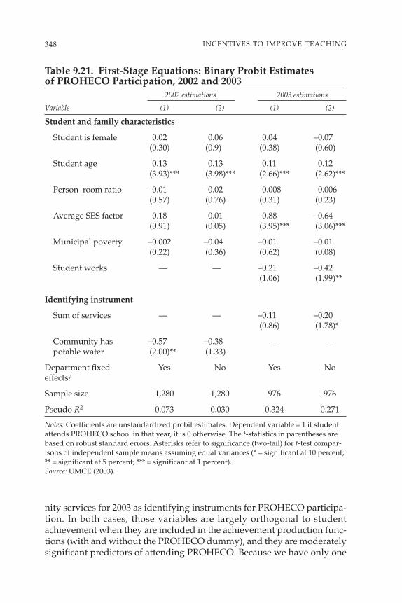
nity services for 2003 as identifying instruments for PROHECO participa-tion. In both cases, those variables are largely orthogonal to studentachievement when they are included in the achievement production func-tions (with and without the PROHECO dummy), and they are moderatelysignificant predictors of attending PROHECO. Because we have only one
348 INCENTIVES TO IMPROVE TEACHING
Table 9.21. First-Stage Equations: Binary Probit Estimates of PROHECO Participation, 2002 and 2003
2002 estimations 2003 estimations
Variable (1) (2) (1) (2)
Student and family characteristics
Student is female 0.02 0.06 0.04 −0.07 (0.30) (0.9) (0.38) (0.60)
Student age 0.13 0.13 0.11 0.12(3.93)*** (3.98)*** (2.66)*** (2.62)***
Person–room ratio −0.01 −0.02 −0.008 0.006 (0.57) (0.76) (0.31) (0.23)
Average SES factor 0.18 0.01 −0.88 −0.64 (0.91) (0.05) (3.95)*** (3.06)***
Municipal poverty −0.002 −0.04 −0.01 −0.01 (0.22) (0.36) (0.62) (0.08)
Student works — — −0.21 −0.42 (1.06) (1.99)**
Identifying instrument
Sum of services — — −0.11 −0.20 (0.86) (1.78)*
Community has −0.57 −0.38 — —potable water (2.00)** (1.33)
Department fixed Yes No Yes Noeffects?
Sample size 1,280 1,280 976 976
Pseudo R2 0.073 0.030 0.324 0.271
Notes: Coefficients are unstandardized probit estimates. Dependent variable = 1 if studentattends PROHECO school in that year, it is 0 otherwise. The t-statistics in parentheses arebased on robust standard errors. Asterisks refer to significance (two-tail) for t-test compar-isons of independent sample means assuming equal variances (* = significant at 10 percent;** = significant at 5 percent; *** = significant at 1 percent).Source: UMCE (2003).

identifying instrument for each estimation, it is not possible to cannot do abetter job of assessing instrument validity (such as incorporating a testfor overidentification).
The results in table 9.21 highlight some of the difficulties involved inpursuing sexy econometric solutions to selection issues. Few parametersare significant predictors of PROHECO school attendance, although, ingeneral, the parameter signs are in the right direction. In 2002, the pro-portion of explained variance is very low, which will have the effect ofcompressing the variance in the predicted parameter for PROHECO par-ticipation. The identifying instruments are generally significant but notvery robust predictors. Finally, the results are somewhat sensitive to theinclusion of the department fixed effects, especially in 2003 when thePROHECO and Control samples were not equalized by geography.
Using the parameters from table 9.21, we calculated predicted proba-bility of PROHECO attendance for each student. We then reestimatedthe production functions from tables 9.17, 9.18, and 9.19 using this pre-dicted parameter. The full results do not change much, so to save space,the only parameters that are presented in table 9.21 are the PROHECOcoefficients.
The results in table 9.22 are underwhelming. In general, the value ofthe predicted PROHECO parameter is larger than the actual parametertaken from the (nearly) identical estimations in tables 9.17–9.19. Thisfinding implies that selection bias is an issue, and the nature of the biasis to underestimate the true effect of PROHECO. In other words, the
349TEACHER EFFORT AND SCHOOLING OUTCOMES
Table 9.22. Comparison of PROHECO Achievement EffectUsing Predicted and Actual Measure of PROHECOParticipation, 2002 and 2003
2002 2003
Variable Predicted Actual Predicted Actual
Spanish 6.71 3.21 5.54 2.63(0.63) (1.75) (0.25) (1.04)
Mathematics 10.05 4.03 11.17 3.80(0.95) (2.67) (0.46) (1.50)
Science 2.97 2.00 17.72 5.74(0.30) (1.06) (1.10) (2.45)
Notes: PROHECO parameter taken from regression with individual and family controlsonly. Same estimations as estimation 2 in tables 9.17–9.19. Predicted refers to nontrans-formed (namely, inverse Mills ratio) predicted probability of being PROHECO school takenfrom estimations presented in table 9.21. Asymptotic t-statistics in parentheses are based onrobust standard errors.Source: UMCE (2003).

characteristics of students who attend either PROHECO or the schoolsthemselves are negatively correlated with unobservable factors that leadto better outcomes. The key implication from table 9.22 is that, with moredata measuring other influences, the effect of PROHECO on achievementshould increase.
Those estimates using selection correction techniques represent a firstcut at this issue. The sample sizes are small, the identifying instrumentsare not particularly convincing, and the results are fairly sensitive to theinclusion of the department dummies. Nevertheless, despite these con-cerns, these results do provide some support for interpreting the signifi-cant PROHECO parameters in tables 9.17–9.19 as indicators of PROHECOeffectiveness.
In addition to doing the sample selection bias analysis using Heckman-style correction techniques, we conducted additional analyses usingpropensity score matching. The propensity score method proceeds in twostages. In the first stage, the 0–1 treatment is regressed onto control vari-ables, and the cases are then put into blocks that are based on ranges of thepropensity to be treated. The key to this phase is the balancing, where foreach block, roughly equal numbers of treatment and control group casesmust be included. Conditional on being balanced, the first-stage regressioncreates a variable that is the propensity score, which is included in thesecond-stage analysis of average treatment effect (ATE). For this secondphase, a series of estimators is available to match treatment and controlcases that are based on their propensity scores, including nearest neighbor,kernel matching, radius matching, and so forth. Because of small num-bers of matching cases, bootstrapped standard errors are sometimes nec-essary, especially with small samples (like ours).
The results from our analysis for 2002 and 2003 in all three subjects aresupportive of a positive treatment in PROHECO. This finding is consistentwith our other analyses, including the Heckman-style model, although thesize of the PROHECO effect is generally smaller and less significant thanwhat was found elsewhere. However, the propensity score treatmentmethod does not appear to be the best “fit” for our particular treatmentanalysis. Why? The main problem is that, because of the balancing require-ment in the first-stage regression, we are left with a very narrow compar-ison to be made in the second-stage ATE analysis. To achieve balancing, wefound it necessary to restrict the first-stage propensity score generation toa very small group of independent variables—even smaller than what wasused in the Heckman model. In effect, this restriction means that we inter-preted the second-stage treatment analysis as the difference in achievementconditional on student gender, age, and some (not all) of the remaininghousehold characteristics (including average SES for the school). None ofthe department dummies were included. As a result, this first-stage regres-sion has little predictive power.
350 INCENTIVES TO IMPROVE TEACHING
All of this explanation means that the PROHECO effect is a ceterisparibus treatment effect that is based on very little in the way of condition-ing variables. So unsurprisingly, the treatment effect—though consistentlypositive—is not very big. By failing to control for other things that aredifferent between PROHECO and control schools—like teacher educa-tion, experience, and so forth—our treatment effect, which we expect tobe largely a function of teacher effort, is partly washed out by the otherdifferences.
This description is one explanation, anyway. Because we are new to thisparticular technique, user error may be another factor. But it also seemsplausible that, with small samples and collinear predictors, the propen-sity score analysis is simply too sensitive to allow us to base policy rec-ommendations on it. For now, the conclusion we make here is probably thesafest one to make.
Student FlowsWe have more data to exploit on student outcomes than just test scores.For a program such as PROHECO, we need to recognize both the possi-bility that PROHECO schools affect things other than achievement andthe possibility that those other differences confound our analysis of testscores. Those possibilities and the way they might affect our analysis havealready been referred to in the discussion on selection bias and in theprevious section. Here, we turn to some of those additional student out-comes as dependent variables.
Table 9.23 details the determinants of student absences. In estimation 1for each year, the basic student and family SES controls are included as pre-dictors (and are presented). For estimation 2, the full model correspondingto the earlier production function work for achievement is estimated (but isnot presented). All models include controls for the departments. In both2002 and 2003, students were asked how many days they had missed dur-ing the school year. Their responses are grouped into an ordered categori-cal variable. As a measure of student attendance, this grouping isproblematic because students may feel a need to underestimate the num-ber of days they have missed. We also know nothing about how manydays the school was open, which forces us to treat the absences as beingthe same in percentage terms.
We used an ordered probit model, given the ordered nature of thedependent variable. The results do not change much when we use ordi-nary least squares regression. One limitation of the ordered probit is thatthe resulting coefficients are very hard to interpret and depend on the den-sities in each of the categories.
No evidence indicates that PROHECO schools have succeeded inreducing student absences. The results in table 9.23 show that not much
351TEACHER EFFORT AND SCHOOLING OUTCOMES

352 INCENTIVES TO IMPROVE TEACHING
Table 9.23. Ordered Probit Estimates of Student-ReportedAbsences, 2002 and 2003
2002 estimations 2003 estimations
Variable (1) (2) (1) (2)
PROHECO school −0.07 0.08 0.06 0.24 (0.61) (0.50) (0.58) (1.34)
Student and family characteristics
Student is female −0.04 −0.05 −0.03 −0.02 (0.61) (0.72) (0.34) (0.23)
No preschool 0.08 0.13 0.04 0.05 (0.99) (1.38) (0.68) (0.95)
Repeating grade 0.12 0.14 0.16 0.17 (1.06) (1.21) (1.44) (1.40)
Commuting time — — 0.005 0.004 (2.31)** (2.17)**
Homework help 0.10 0.09 0.21 0.20 (1.31) (1.05) (2.41)** (2.24)**
Person–room ratio −0.008 −0.02 0.006 0.008 (0.43) (0.75) (0.39) (0.48)
SES factor 0.11 −0.11 −0.05 −0.05 (2.12)** (2.27)** (1.07) (1.02)
Student works — — 0.18 0.16 (1.85)* (1.63)
Community characteristics
Average SES factor −0.07 −0.12 0.07 0.04 (0.83) (1.26) (0.88) (0.38)
Remaining school– No Yes No Noteacher controls?
Department fixed Yes Yes Yes Yeseffects?
Sample size 1,203 1,203 939 939
Pseudo R2 0.026 0.035 0.027 0.033
Notes: Dependent variable is an ordinal measure of student-reported absences. Asymptotict-statistics in parentheses are based on robust standard errors. All estimations use fixedeffects at department level. Asterisks refer to significance (two-tail) for t-test comparisonsof independent sample means assuming equal variances (* = significant at 10 percent; ** = significant at 5 percent).Source: UMCE (2003).

of anything significantly predicts this particular outcome, which is notvery surprising given the difficulty of getting clean data on attendance.Some interesting results do occur, however, namely, that commuting time,student work, and family SES significantly affect absences (in the expecteddirection).
Our final outcome is a more direct measure of student flow rates anduses the school-reported information on repetition and dropout rates.For those outcomes, the data are collected by grade and then are pooledfor each school, which results in more than six observations for eachunit (school).
The results in table 9.24 show that, in 2002, PROHECO has no signifi-cant effect on student repetition, but for dropout, PROHECO has a mod-erately significant (negative) effect. Of the two control years, 2002 is clearlythe most problematic because those data refer to the 2002 school year andnot the 2003 year. We have the same problem with test scores, of course,because the exams were applied in different years. But an intertemporaleffect for those outcomes seems more likely.
So the focus should probably be on 2003. The results are encouragingfor PROHECO because they show improvements in repetition anddropout rates, even if the point estimates are not really significant. Theremaining parameters are generally in the expected direction. Because wepooled the data, it is necessary to include intercept controls for eachgrade, and the results corroborate what is already known about inter-grade variation in the outcomes: With each successive grade, less repeti-tion and dropout occurs. But we know nothing about interyear dropoutwith those data, so we urge some caution.
Conclusions
Three general conclusions are supported by the empirical work conductedin this paper. First, PROHECO schools are different from their public-school counterparts. Those differences are generally consistent with whatwe should expect, although not on all accounts. For example, PROHECOschools appear to be open more frequently and have people working morehours. Other differences, however, are less “positive.” In particular, wehave found that PROHECO teachers have fewer educational qualificationsand complain about delays in payments, which suggests that the teachermanagement model is not leading to a better-suited teacher selectionapproach or to a more efficient payment model—in contrast to what wemay have expected.
Additionally, we did not uncover substantial differences in either class-room processes or teaching and learning environments. Those are, to besure, very difficult data to collect and measure with accuracy. Yet the
353TEACHER EFFORT AND SCHOOLING OUTCOMES
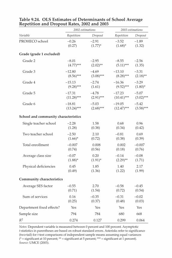
Table 9.24. OLS Estimates of Determinants of School AverageRepetition and Dropout Rates, 2002 and 2003
2002 estimations 2003 estimations
Variable Repetition Dropout Repetition Dropout
PROHECO school −0.26 −2.91 −3.52 −1.89 (0.27) (1.77)* (1.68)* (1.32)
Grade (grade 1 excluded)
Grade 2 −8.01 −2.95 −8.55 −2.56 (4.77)*** (2.02)** (5.11)*** (1.35)
Grade 3 −12.80 −4.69 −13.10 −3.31 (8.56)*** (3.08)*** (8.28)*** (2.18)**
Grade 4 −15.13 −2.74 −16.36 −3.29 (9.28)*** (1.61) (9.52)*** (1.80)*
Grade 5 −17.31 −4.78 −17.23 −5.07 (11.28)*** (2.91)*** (10.41)*** (3.02)***
Grade 6 −18.81 −5.03 −19.05 −5.42 (13.24)*** (2.68)*** (12.47)*** (3.58)***
School and community characteristics
Single teacher school −2.28 1.58 0.68 0.96 (1.28) (0.38) (0.34) (0.42)
Two teacher school −2.50 2.10 −0.81 0.69 (1.66)* (0.72) (0.38) (0.39)
Total enrollment −0.007 0.008 0.002 −0.007 (0.74) (0.56) (0.18) (0.76)
Average class size −0.07 0.20 −0.14 −0.08 (1.88)* (1.91)* (2.29)** (1.71)
Physical deficiencies 0.45 1.85 1.40 2.17 (0.49) (1.36) (1.22) (1.99)
Community characteristics
Average SES factor −0.55 2.70 −0.58 −0.45 (0.71) (1.54) (0.72) (0.54)
Sum of services 0.16 −0.35 −0.31 −0.02 (0.25) (0.37) (0.48) (0.03)
Department fixed effects? Yes Yes Yes Yes
Sample size 794 784 680 668
R2 0.274 0.127 0.299 0.064
Notes: Dependent variable is measured between 0 percent and 100 percent. Asymptotic t-statistics in parentheses are based on robust standard errors. Asterisks refer to significance(two-tail) for t-test comparisons of independent sample means assuming equal variances (* = significant at 10 percent; ** = significant at 5 percent; *** = significant at 1 percent).Source: UMCE (2003).

finding still deserves mention because it forces us to consider the mech-anisms that will predict PROHECO school “success.” The picture that isformed in our analysis is one of PROHECO schools making better useof existing capacity, mainly by having teachers work more and by limit-ing class sizes. According to our data, however, it is not the case thatPROHECO teachers are more effective in the classroom.
Should we even expect differences in classrooms? In theory, theanswer is yes because the community school’s “responsiveness” to itsusers should turn up in differences in curriculum and teaching methods.Our data on this question are incomplete both in terms of qualitativeprocesses and parental involvement. But we need to consider anotherscenario where community school parents limit their oversight to themost visible aspects of teacher effort—teachers’ attendance and hoursworked—without entering classrooms and instigating changes in teach-ing methodology and classroom management. In other words, commu-nity parent councils may not be striving to create the best schools; theymay simply want the most efficient schools.
Our second main finding is that differences in PROHECO school capac-ity use explain a substantial proportion of the observed differences in aca-demic achievement between PROHECO and control schools. In particular,PROHECO schools make better use of existing capacity, mainly by hav-ing teachers work more and by limiting class sizes, thereby confirming theexistence of a link between community schooling and classroom processvariables such as days attended, frequency of homework, and individual-ized learning.
This finding is subject to concerns about selection bias, which weaddress in the empirical work, although only imperfectly. Overall, ourresults show that selection bias is an issue, but that the nature of the biasis to underestimate the true effect of PROHECO. In other words, withmore data measuring other influences, the effect of PROHECO onachievement should increase. Essentially, teacher and school selectiontend to underestimate the PROHECO effect, providing support forinterpreting the significant PROHECO parameters as indicators of PROHECO effectiveness. Additionally, we also find no evidence ofcohort selection bias.
The link between capacity use differences and student outcomes isencouraging, and it provides prima facie support for PROHECO schoolingon pure efficiency grounds. This support is especially true when we con-sider that PROHECO teachers are paid less and have fewer qualifications.Nevertheless, we should avoid concluding that PROHECO schools are morecost-effective, especially given the large differences in student–teacher ratiosand unmeasured aspects of parental involvement. A calculation of theexact cost per student in PROHECO and non-PROHECO schools wouldallow us to make a cost-effectiveness comparison.
355TEACHER EFFORT AND SCHOOLING OUTCOMES

Our conclusion is actually less of a conclusion and more of an appeal. Weneed to know more about what parents want in community schools andhow they go about making their desires reality. Data that will be availablelater in the year hold the promise of addressing those questions. It is easy toassume that parent councils want what is best for their children and thenact accordingly. But what do we really know about what groups of ruralHonduran parents want from the local school and schooling in general?Furthermore, how do they collect information about what is happening intheir schools? We can get at those questions in an indirect way with quan-titative data. Future efforts should improve the quantitative data frame-work while expanding qualitative investigations.
356 INCENTIVES TO IMPROVE TEACHING
References
Bedi, A. S., and J. H. Marshall. 2002. “Primary School Attendance inHonduras.” Journal of Development Economics 69(1): 129–53.
Fuller, B., and M. Rivarola. 1998. “Nicaragua’s Experiment to DecentralizeSchools: Views of Parents, Teachers and Directors.” Working Paper onImpact Evaluation of Education Reforms 5. World Bank, Washington, D.C.
Hadi, A. S. 1992. “A New Measure of Overall Potential Influence in LinearRegression.” Computational Statistics and Data Analysis 14: 1–27.
Jimenez, E., and Y. Sawada. 1999. “Do Community-Managed SchoolsWork? An Evaluation of El Salvador’s EDUCO Program.” World BankEconomic Review 13(3): 415–41.
Marshall, J. H. 2003. “School Attendance and Academic Achievement: ASimultaneous Equations Approach.” Stanford University, Stanford,Calif. Processed.
Marshall, J. H., and K. A. White. 2002. “Academic Achievement, SchoolAttendance, and Education Policy in Honduras.” Stanford University,Stanford, Calif. Processed.
McEwan, P. J., and J. H. Marshall. 2004. “Why Does Academic AchievementVary across Countries? Evidence from Cuba and Mexico.” Education Eco-nomics 12(3): 205–17.
Sawada, Y. 1999. “Community Participation, Teacher Effort, and Educa-tional Outcome: The Case of El Salvador’s EDUCO Program.” WilliamDavidson Institute Working Paper 307. University of Michigan Busi-ness School, Ann Arbor.
UMCE (Unidad de Medición de la Calidad Educativa), UniversidadPedagógica Nacional Francisco Morazán (UPN), and Secretaria deEducación (SE). 2003. “Informe nacional de rendimiento academico2002.” Tegucigalpa, Honduras. Processed.
357


10Teacher Incentives and Student
Achievement in NicaraguanAutonomous Schools
Caroline E. ParkerEducation Development Center, Inc.
This chapter looks at Nicaragua’s decentralization program, known asautonomy, through the lens of teacher incentives and student achieve-ment. Although there have been numerous studies to date on Nicaraguanautonomy, most of them have focused on the decentralization of decision-making. Few studies have looked at what effects decentralization has onteacher behavior and whether changes in teacher behavior have an effecton student achievement. This chapter considers the following question:Have the changes in autonomy, particularly those related to teacher incen-tives, led to improved student outcomes?
To address that question, the chapter first describes the national contextof Nicaragua’s education reform, next considers the analytic frameworkand the methods of the study, and then answers the research question.
Nicaraguan Context
Nicaragua, a country of 5.3 million people, has 2.2 million children andyouth of school age. The average age of Nicaraguans is 22 years, which hasbeen rising for the past 10 years, but still ranks the country as having theyoungest population in Latin America. The average total education forNicaraguans is 4.6 years. Adult illiteracy rates range around 33 percent,and 36.8 percent of the adult population does not have a complete primaryeducation; 71.5 percent of adults have not completed secondary education.Sixty percent of teenagers are not in the education system. Only 4.7 percent
359
I would like to thank Maria Martiniello, Patrick McEwan, Andrew Ballard Ragatz, LucreciaSantibáñez, Yasuyuki Sawada, and Emiliana Vegas, for their comments, as well as the mem-bers of the April 22 Workshop. I would also like to thank Reyna López of the NicaraguanMinistry of Education for providing valuable assistance.

of the adult population has university degrees (MECD 2003b). Thus, thisstudy of educational change and quality takes place in the context of lessthan full access to all tiers of education. Nicaragua, like other developingcountries in the 21st century, must address issues of school quality con-currently with addressing issues of access—a forbidding challenge(Tedesco and López 2002).
Nicaragua also faces educational challenges amid long-term social andpolitical upheaval. Economically, although Nicaragua has been experi-encing growth over the past 10 years, the slowness of the growth meansthat many Nicaraguans continue to be poor: 46 percent live in poverty,with 15 percent in extreme poverty (MIGOB 2003). Nicaraguans’ percapita income ranges around US$700 annually. Official unemployment is11.3 percent, but of the employed, 64 percent are in precarious jobs (infor-mal sector) and 33 percent are underemployed (MIGOB 2003). The coun-try’s generalized poverty means that both the government and individualfamilies have extremely limited resources to invest in education.
Nicaraguan Autonomy
Among the education reforms sponsored by the Nicaraguan Ministry ofEducation, Culture, and Sports (MECD) during the past 15 years is a school-based reform of management decentralization known as autonomy. Begunin 1993, the school-based management model had three goals (Castillo1998):
1. Increase community participation in educational administration.2. Obtain financial resources for schools beyond government funding.3. Increase efficiency in the use of human and financial resources for
schools.
The decentralization began within a political framework of “returningeducation to local communities” (Arcia and Belli 2001). However, a recentqualitative analysis of autonomous schools found that the reform has notreconstructed the social pact to increase parents’ role in their children’seducation. Instead, it has a “financial-administrative” focus (Asencio andothers 2001, p. 6). The MECD first decentralized the 20 largest secondaryschools in Managua, hoping that they would become a model of auton-omy for other schools. The autonomy process continued to expand through2000. There were experiments with municipal decentralization in ruralareas, and there continue to be various iterations of school-based manage-ment. In 2002, 37 percent (1,781) of all Nicaraguan primary and secondaryschools were autonomous (MECD 2004). Autonomous schools served 63 per-
360 INCENTIVES TO IMPROVE TEACHING
129. These numbers differ slightly from numbers in other MECD data.

cent of students (501,000) and had 13,419 teachers (MECD 2004).129 Of472 public secondary schools, 331 were autonomous (MECD 2003a). Of the252,000 public secondary school students in 2002, only 42,000 were servedoutside the autonomous school system.
In the original autonomy reform, improving educational quality was notamong the top three goals. The underlying assumption, however, was thatby increasing community participation, improving a school’s financial sta-tus, and improving efficiency, the final result would be higher-quality edu-cation. The following section carefully examines the history and currentstatus of autonomy as background for answering the primary researchquestion of whether students in autonomous schools perform better thanthose in centralized schools.
Community Participation
Autonomy, or school-based management, gives greater decisionmakingpower to school directors, teachers, and parents. Autonomous schoolsform school councils made up of parents, teachers, the school director, anda nonvoting student representative. Parents and teachers are selected invarious ways, ranging from general elections to appointment by a localmayor or MECD delegate (Gershberg 2003). The autonomous school coun-cil hires and fires teachers and the director; designs the annual plan;approves school rules; modifies the curriculum within Ministry of Educa-tion, Culture, and Sports standards; and authorizes the budget (Castillo1998). In reality, school directors dominate school councils in many schools(Castillo 1998; Fuller and Rivarola 1998; King 1996), and parents and teach-ers have less participation than originally envisioned. Decentralizationdoes appear to be related to greater local decisionmaking at autonomousschools, but evaluations have been mixed about the participation level onschool councils. Neither parents nor teachers generally feel that they havemuch authority, but directors have said that they feel they have greaterability to make decisions (di Gropello 1997; King 1996). The extent of par-ticipation by stakeholders appears to depend on the leadership style of theschool director (Asencio and others 2001; Asencio Florez and others 2001).Teacher participation appears to wane when teachers’ financial incentivesare smaller (Gershberg 2003; Gershberg and Winkler 2000).
Finance
The most contentious of the three goals in the autonomy process were thefinancial aspects (Gershberg 2003). Antidecentralization activists empha-sized the privatizing characteristics of charging for public education. Formany poor Nicaraguans, autonomy did, indeed, seem like another wordfor privatization. Although autonomy encompasses far more than simply
361TEACHER INCENTIVES AND STUDENT ACHIEVEMENT

the parent’s financial commitment to a child’s education, the monthly feewas foremost in parents’ minds in Nicaragua’s crisis economy (Fuller andRivarola 1998). In 1995, the government determined, through a constitu-tional amendment, that autonomous primary schools could not chargeobligatory fees, but secondary schools were allowed to charge up to a cer-tain amount (about US$2 monthly) in obligatory fees (Castillo 1998; Fullerand Rivarola 1998). This resolution meant that all secondary schools couldcharge monthly fees, and critics continued to predict that the policy wouldexacerbate educational inequities. In 2002, however, new legislation,which for the first time legalized school-based management, eliminatedthe right to charge fees. Thus, by law, neither primary nor secondaryschools may charge obligatory fees for attendance, although they maystrongly encourage voluntary donations.
The MECD has two funding structures: one for nonautonomous (cen-tralized) schools and one for autonomous schools. The ministry directlypays all the costs of the centralized schools. For the autonomous schools, itpays each school on a per student basis and on a sliding scale that wasimplemented in July 2002, by which smaller schools get more per studentthan larger schools. The monthly amounts range from about 78 córdobas(US$6) for small schools to 52 córdobas (US$4) per student for largeschools (Morales 2002). Proactive directors can seek outside donations andget external funding from both national and international sources. Becauseschools may no longer charge obligatory fees, the ministry recognizesthat one of its challenges is to make sure that no schools are prohibitingentrance on the basis of ability to pay fees. In addition to per student fund-ing sent to each school, teachers get a twice-yearly bonus from the govern-ment. The bonuses are currently funded by the World Bank and dependon the number of students in each classroom. The bonus is supposed toencourage teachers to work hard on student retention. In 2003, 16,000teachers in autonomous schools received the biannual bonus, among atotal of 31,000 teachers in the entire system (autonomous and centralized).The bonus in 2003 averaged 800 córdobas (about US$52).
Centralized schools have a different funding structure. The ministrypays all their expenses—water bill, electric bill, teacher salaries, and so on.Less of a relationship exists between the number of students and how mucha school receives. Teachers in autonomous schools can be let go if they donot have at least 35 students in their classroom, which is not the case in cen-tralized schools. About 15,000 teachers are not in the autonomous system.
Many of the schools that initially chose autonomy convinced theirteachers that it would lead to higher salaries, because the increased free-dom to charge fees would improve their financial situation. In this way,the ministry saved money at the central level, and, theoretically, schoolsobtained more money for school improvements (Arnove 1995). Thus,whereas parents often equated autonomy with privatization, teachers
362 INCENTIVES TO IMPROVE TEACHING

often equated it with improved salaries (accompanied by less job stability).When the MECD eliminated obligatory fees in 2002, some teachers inter-viewed described the change as the end of autonomy because it was theend of their monthly, school-based bonuses. In practice, many primaryschools, especially those in poor and rural areas, had eliminated the obli-gatory fees well before 2002, and the financial benefits of autonomy had allbut disappeared for teachers (Asencio and others 2001). In contrast, somesecondary schools have continued charging fees despite the legal mandateagainst them (Asencio and others 2001).
In 2003, the annual educational budget reached US$100 million, whichrepresents almost 4.5 percent of Nicaragua’s gross domestic product. How-ever, this figure averages only US$72 per student throughout the system. Ofthe budget, 76 percent goes toward teacher salaries. Almost 20 percent ofthe educational budget comes from foreign loans.
Efficiency
The third goal of Nicaraguan autonomy was efficiency. By transferring fis-cal responsibility and decisionmaking to the school level, school directors,school councils, and teachers would become accountable directly to par-ents, thus increasing the ability of stakeholders to directly affect educa-tion. Among others are three ways in which improved efficiency can target,in particular, teacher behaviors: teacher incentives, increased resources, andprofessional development.130
Primary school teachers earn an average of US$111 monthly, about 70 percent of the government-determined market basket (MECD 2003b).They have, on average, 11 years of education, equivalent to a high schooldegree. Secondary school teachers have an average of 13 years of educa-tion and earn an average of US$117 monthly (MECD 2003b). Most pri-mary school teachers are trained at normal schools, which are teachertraining institutes. In 2000, 73.6 percent of teachers reported having therequisite teaching certificates from normal schools (MECD 2004). Allnewly hired teachers must have certificates. However, many rural schoolsdo not have enough qualified teachers, and Normal Schools continue to beunder enrolled, indicating that there will continue to be a shortage ofqualified teachers.
IncentivesTeacher incentives have been an important element in decentralizationfrom the beginning of the reform. For a school to become autonomous, 80 percent of teachers must vote in favor of autonomy. One of the biggest
363TEACHER INCENTIVES AND STUDENT ACHIEVEMENT
130. Although decentralization of decisionmaking has been a key element of Nicaraguanautonomy, this data set does not include questions about decisionmaking.

selling points for teachers was the promise of higher salaries throughbonuses and incentives. Teachers faced lower job security, however,because in autonomous schools the councils hire and fire teachers. Thus,teachers without at least 35 students in their classroom can be let go.Autonomous schools can give their teachers incentives from two sources.First, the World Bank funds an incentives program that is based on studentattendance. Teachers receive biannual incentives tied to the number of stu-dents who are registered and who study in their class. Incentives averagealmost a month’s salary. The second form of incentive depends on eachschool’s individual resources. Teachers receive incentives drawn frommonthly fees collected from students. Because autonomous schools kept100 percent of all fees collected but centralized schools kept only 50 per-cent, becoming autonomous brought with it the prospect of increasedincome for schools and, therefore, increased incentives for teachers. In arecent survey of autonomous schools, monthly fees resulted in up to 5 per-cent additional revenue for the school. Generally, half of this revenue isgiven to teachers, half to school maintenance. Teachers in autonomous pri-mary schools receive from 0 to 30 percent of their salary in bonuses, whilein secondary schools they earn from 0 to 50 percent (Gershberg 2003).
Infrastructure and Material ResourcesBecause of their greater financial independence, autonomous schools alsohave potentially more resources and better-quality infrastructure. In theearly years, autonomous schools often received government or inter-national funding. The World Bank has funded a US$14 million educationprogram that has targeted funds to autonomous schools. Directors ofautonomous schools are encouraged to seek alternative sources of fund-ing, both in the local community and through international contacts. Like-wise, one of the school council’s stated responsibilities is to diversifyfinancial sources for the school. Thus, autonomous schools would be likelyto have more resources than centralized schools.
Professional DevelopmentFinally, teacher professional development has been recognized as a criticalelement in school improvement. Teachers’ salaries are the single greatestexpense for the MECD, and efficient use of those resources includes improv-ing the quality of teaching through further education and training for thoseteachers. The initial stages of the autonomy reform did not emphasize pro-fessional development, and the MECD continues to provide professionaldevelopment to all schools, centralized and autonomous. Autonomousschools have the potential to provide more and better-quality professionaldevelopment, although no studies to date have identified whether they doso. In addition, autonomous schools may theoretically choose their own cur-
364 INCENTIVES TO IMPROVE TEACHING

riculum. However, they rarely do so in practice (Asencio and others 2001;Asencio Florez and others 2001).
Autonomy Today
School autonomy was institutionalized with the “Educational Participa-tion” law of May 2002. The major elements of the new law include thefollowing (MECD 2003c):
• No schools may charge obligatory fees (although schools continue to beresponsible for all school finances).
• The name “autonomous schools” has been eliminated, and autonomousschools are now termed “schools of educational participation.”131
• All schools must become schools of educational participation by May2006 (although there are no funds for schools to implement decentral-ization, and there have been no new autonomous schools since 2001).
• There is a renewed emphasis on developing school councils and com-munity councils. School councils administer all funds; they hire and fireteachers and principals.
• The decentralization structures, including the funding process, are apart of school structures.
• Autonomous schools receive per student funding.• The school director and school council have financial and administra-
tive responsibilities.• Parents have an active role in decisionmaking through the school councils.• Directors have academic development responsibilities.
A recent evaluation of autonomous schools found that “the AutonomousSchool is a concept that is not sufficiently understood” (Asencio and others2001, p. 8). Throughout my study of the effects of decentralization on teacherpractice, I have kept in mind that definitions of autonomy vary by school,that the implementation of autonomy varies by school, and that recentlegislation has legalized some aspects of autonomy while changing otherssuch as the name. Although school-based management may be clearlydefined on paper, in practice there is great variation within Nicaraguanschools.
Previous Studies of Nicaraguan Autonomy
Nicaraguan autonomy has been studied from numerous angles. Somestudies focus on governance issues and look at shifts in decisionmaking
365TEACHER INCENTIVES AND STUDENT ACHIEVEMENT
131. In my study, decentralized schools will be referred to as autonomous schools becausethe terminology continues to be in common use in Nicaragua. Nonautonomous schools arereferred to as centralized schools.

(Arnove 1995; Gershberg 1999a; King 1996; King, Ozler, and Rawlings2000). Others focus on finance (Gershberg 2003; Gershberg and Meade2003); on equity (Castillo 1998; di Gropello 1997; di Gropello and Cominetti1998); on parental involvement (Fuller and Rivarola 1998; Gershberg 1999a,1999b); and finally, on student outcomes (King and Ozler 2000).
This chapter contributes to the literature on student outcomes. It attemptsto address some of the methodological challenges faced by King and Ozler(2000) in their previous study of student outcomes (discussed in theMethods section that follows). It looks more closely than previous studiesdo at what teachers’ characteristics are and at what happens in the class-room. It uses the first wave of an important new data set that is the most-comprehensive study of student achievement to date in Nicaragua.
The autonomy process has been a far-reaching reform that has touchedmany aspects of the educational process in Nicaraguan primary and sec-ondary schools. However, any study of the effects of autonomy mustremember the following:
• Overall funding for public schooling in Nicaragua continues to be verylow, and there is a risk that it has not yet reached a threshold of spend-ing that can significantly and positively affect student outcomes. Withonly US$72 per student, there may simply not be enough resources toprovide professional development, materials, and infrastructure thatwill allow any school—whether decentralized or not—to improve stu-dent performance.
• Despite being a reform that is now 10 years old, autonomy has experi-enced several significant challenges that may affect its ability toimprove student performance:
� Proponents of autonomy spent many years fighting accusations ofprivatization and were placed in a defensive position rather thanbeing able to promote community participation.
� The initial emphasis on financial autonomy led many schools tofocus almost exclusively on financial aspects, to the detriment ofschool improvement.
� The new educational participation law in 2002 has led to some con-fusion because of the elimination of the term “autonomy.” Althoughthe law states that all schools will now have the decentralized char-acteristics of autonomous schools, the change is often interpreted asbeing the end of autonomy.
� Studies have shown that there is generalized confusion over whatautonomy is and what it is supposed to do for schools, teachers, andstudents (Asencio and others 2001).
In summary, although this study separates autonomous from central-ized schools, fewer differences than expected may materialize between auto-
366 INCENTIVES TO IMPROVE TEACHING

nomous and centralized schools, even after 10 years of reform. In the contextof Nicaraguan education, asking whether autonomy has led to improve-ments in student outcomes may be the wrong question. The correct questionwould identify which school characteristics are associated with improvedstudent outcomes and would use that information for policy development.This study asks the first question and concludes with implications for thesecond.
Methods
Analytic Framework
This study uses impact evaluation methods, which involve establishing acounterfactual state (centralized schools) against which the current state(autonomous schools) will be compared. The research question considersthe effect of school characteristics and teacher behavior on student achieve-ment, in this case on Spanish and math scores. The multilevel model esti-mates the effect of the dummy variable autonomy (A) on student outcomes(Y) for student i in the classroom of teacher j. The model controls forobserved characteristics of students (S) and for teacher characteristics (T).The relationship can be written as
Although the multilevel model addresses the nesting issue and is ableto identify the teachers’ characteristics, it does not address the bias of sam-ple selection. Previous analysis of data looking at student outcomes inNicaraguan autonomy (King and Ozler 2000) has been subject to criticismbecause of its statistical procedures (Kaestner and Gershberg 2002). Kingand Ozler used panel data that matched autonomous and centralizedschools, collected data on schools and individuals, and administered mathand Spanish tests to a randomly selected group of students in the fourthgrade and in the third year of secondary school. They faced two significantchallenges with these data: a very large attrition rate of almost 50 percent(Kaestner and Gershberg 2002) and sample selection bias. Because schoolsare not randomly assigned to autonomous status and students are not ran-domly assigned to schools, any study of differences between autonomousand centralized schools can suffer from selection bias. Despite King andOzler’s use of instrumental variables estimation to address this challenge,the results have been open to criticism.
The data set used in my analysis does not have the problem of attrition,but it does face the same challenges of selection bias. Schools were not ran-domly chosen to be autonomous; thus, those schools that became auton-omous may share certain characteristics beyond autonomy that contribute
Y S Tij j j i j ij= + + + +α β β β ε1 2 3(Autonomous)
367TEACHER INCENTIVES AND STUDENT ACHIEVEMENT

to student outcomes (some that have been suggested include student char-acteristics of socioeconomic status or parent education, or school character-istics of director skills or teacher quality). To address this potential bias, I havechosen propensity score matching using stratification and nearest-neighbormatching. There are two levels of selection bias. The first is at the school level,because certain types of schools may be more likely to become autonomousthan others. The second is at the student level, because in areas where thereare both autonomous and centralized schools, certain types of students maybe more likely to attend autonomous schools over centralized schools.
Because I am interested in student outcomes, I have conducted thepropensity score matching at the student level, including appropriateteacher-level variables. In addition, the variables that best contribute todeveloping a propensity score are those that can be expected to be associ-ated both with participation and with the outcome. At the student levelthose variables are socioeconomic status and student age. At the schoollevel, the variables could be teacher years of education and teacher experi-ence, but neither of those variables is significantly different betweenautonomous and centralized schools in the studies. Other school-level vari-ables that are significantly different include incentives, teachers’ view ofschool conditions, and directors’ provision of professional development. Iargue that by using propensity score matching, I address the limitations ofselection bias and that my outcomes reflect more accurately the differencesbetween autonomous and centralized schools. I report results using multi-level modeling without correcting for selection bias, as well as results usingstratification and nearest-neighbor matching with propensity scores.
Statistical Analysis
The model in this paper builds on the premise that autonomy has led tochanges in teacher incentives; that the changes in teacher incentives haveled to changes in teacher behavior; and that those changes, in turn, have ledto improved student achievement. I test the hypothesis with the equationdescribed in the Analytic Framework section earlier. The variables wereplaced into one of the following clusters: three control variable clusters—student-level characteristics, classroom characteristics, and school charac-teristics; and three question clusters—incentives, infrastructure andmaterials, and technical assistance. For both the third- and sixth-gradeoutcomes, each of the variable clusters was first tested independently.Then those variables that reached significance were kept in the modeluntil a final model was obtained. The model tables include each of theinitial models and the final model. The models were tested using bothrandom effects and fixed effects. The fixed-effects model captures alldifferences by teacher, rather than just the variables included in themodel. The fixed-effects models do not provide a coefficient for the dif-
368 INCENTIVES TO IMPROVE TEACHING

ference between autonomous and centralized schools. Rather, they helpus to see the overall differences between teachers, regardless of schooltype.
Because the multilevel model does not adequately account for selec-tion bias, propensity score matching was done using both stratificationand nearest-neighbor matching. The propensity score was determined byconsidering which variables contribute to both the treatment (being auton-omous or not) and the outcome. After looking at propensity scores usingvariables from all of the clusters previously described, I chose the propen-sity score using the variables that remain in the final multilevel model.This choice makes sense substantively because the propensity score de-scribes schools that are essentially similar on all the variables of interestand then tests for the difference in means between schools that share sim-ilar propensity scores.132 The differences in results among the three dif-ferent statistical processes are discussed later.
Data
The data were collected as part of a World Bank–funded project, the firstnational study of educational quality, which was administered in 2002 toa nationally representative sample of third- and sixth-grade students. Stu-dents were given tests in Spanish and mathematics. Students, teachers,parents, school directors, and school council members filled out question-naires about their school. The schools were chosen using a stratified ran-dom sample by region, school type, urbanicity, and multigrade modality,thereby allowing analysis at various levels, including school type. All stu-dents in the third and sixth grades were tested (third- and sixth-gradesamples were developed separately). The study encompassed all schooltypes, including private schools that do and do not receive state funding.
Sample
This study uses information from the director, teacher, parent, and studentinterviews, as well as test results from both third- and sixth-grade stu-dents.133 For the purposes of this study, the sample was restricted to onlyautonomous and centralized public schools in order to focus on differ-ences between the two public school models.
Most student scores fall in the basic range. Fewer than 20 percent of stu-dents in any grade level or subject scored proficient. Those results include
369TEACHER INCENTIVES AND STUDENT ACHIEVEMENT
132. The propensity score matching details are available from the author upon request.133. The socioeconomic status variable was built from the parent survey, and student data
on gender and age were taken from the student data.

not only centralized and autonomous schools, but also private subsidizedand private schools, which, on average, have higher scores than publicschools. Overall achievement levels on the Spanish and math assessmentswere low, and many students performed well below grade level (MECD2003a). The tests were designed through extensive consultation with expe-rienced teachers and in accordance with the national standards for Span-ish and mathematics. Thus, the ministry staff considers them to be alignedto the curriculum. The generally low results indicate that students are notlearning what teachers think they are teaching the students. The tests werescored using Item Response Theory (MECD 2003a). In the following sec-tions, I first describe the results obtained using third-grade data, then fol-low with sixth-grade data.
Third-Grade Descriptive Statistics
There are 134 schools in the third-grade study: 52 percent autonomous and 48percent centralized. Of the sections, 80 percent meet in the morning, 20 percent in the afternoon. Of the directors, 63 percent reported using multi-grade classrooms. Among the schools, 71 percent are in rural areas; 29 per-cent are in urban areas. The sample is evenly divided between boys and girls.
The director and teacher interviews asked extensive questions related toincentives, infrastructure and materials, and professional developmentand classroom practice. This conformation permitted the development ofa series of variables that describe director and teacher perceptions andpractice.
As already described, certain uniform governance policies occur acrossautonomous schools, which include government funding formulas, fiscalresponsibility, and the practice of hiring and firing of teachers and direc-tors. Variations exist from school to school in the concrete implementa-tion of autonomy, but this data set does not include a detailed study ofdecisionmaking patterns. Thus, the statistical analyses focus specificallyon those school practices that could have a direct effect on teacher behav-ior, rather than on those governance practices that are most closely asso-ciated with autonomy.
Control VariablesThe statistical analyses control for variables that may affect teacher behav-ior or student achievement but that are not part of the research question.Student controls include student age, student sex, and household socio-economic status (SES). Teacher controls include class size, teacher’s expe-rience, teacher’s years of education, section mean of household SES, sectionmean of age, student absences reported today and last week, and numberof students repeating grade. School control variables include school type,total number of students in school, mean school SES, and urbanicity.
370 INCENTIVES TO IMPROVE TEACHING

The students who attend autonomous schools differ significantly fromthose who attend centralized schools in a number of areas. On average,students in autonomous schools are younger than those in centralizedschools. On average, students in autonomous schools are also wealthierthan those in centralized schools.
Average student absences vary by school type. Teachers reportedmore absent students in autonomous schools (6.17) than in centralizedschools (4.98). Table 10.1 provides descriptive information for all the con-trol variables.
In addition to identifying schools as autonomous or nonautonomous,this study breaks down autonomous schools by the number of years eachhas been autonomous. Table 10.2 shows the breakdown by years.
Question VariablesIncentivesAlthough financial incentives in the form of teacher bonuses are the mostcommon incentive, the questionnaire asked about eight different incen-
371TEACHER INCENTIVES AND STUDENT ACHIEVEMENT
Table 10.1. Control Variables: Third-Grade Mean Values, by School TypeVariable Centralized Autonomous Total
Student characteristics:
Student age*** 9.8 9.6 9.68
Student SES*** −0.308 −0.192 −0.242
Classroom characteristics:
Classroom mean SES −0.593 −0.531 −0.56
Mean age 10.2 10.1 10.15
Mean class size* 25.9 30.6 28.3
Teaching experience 11.7 11.3 11.5
Total years education 12.2 12.2 12.2
Number of students 2.86 2.93 2.89repeating this year
Students absent this week* 4.98 6.17 5.59
Students absent today 3.6 5.8 4.7
School characteristics:
Total students*** 381 916 686
Note: *p < 0.05, ***p < 0.001.Source: Author’s calculations.

tives (financial incentives, job promotions, scholarships for further study,honor roll, medals, school supplies, extra books, and teacher field trips).The question was asked of both the teacher and the director. For this study,the financial incentive variable was used in table 10.3 because it has been—and continues to be—the most common and popular of the incentives.
Both teachers and directors in autonomous schools report higher ratesof financial incentives than the rates in centralized schools. However, it isinteresting to note that although 74 percent of autonomous school direc-tors say that teachers get incentives, only 67 percent of autonomous schoolteachers say they do (table 10.3).
ResourcesFour variables address infrastructure and material resources. The firstis the mean of 30 variables asking teachers about the condition of certain
372 INCENTIVES TO IMPROVE TEACHING
Table 10.2. Years of School Autonomy, Third GradeYears of autonomy Frequency Percentage
Not autonomous 64 48.0
1 9 6.7
2 0 0.0
3 3 2.24
4 29 21.64
5 3 2.24
6 11 8.21
7 15 11.19
Total 134 100.00
Source: Author’s calculations.
Table 10.3. Third-Grade Descriptive Statistics for Incentive Variables
Centralized schools Autonomous schoolsVariable (percent) (percent)
Teacher reports financial incentive*** 22 67
Director reports teacher financial incentive*** 36 74
Note: ***p < 0.001.Source: Author’s calculations.

items at their school, ranging from chalk to computer labs. The last threevariables focus on teaching resources: whether or not teachers haveaccess to the curriculum standards and curriculum guides, and howlong the school has been implementing the new curriculum standards(table 10.4).
Professional DevelopmentFour variables address professional development: whether the directormeets with teachers, whether the director provides technical assistance toteachers, whether the director gives Spanish workshops to teachers, andwhether the director gives math workshops to teachers (table 10.5).
Outcome VariablesStudent scores on the Spanish and math tests were used as outcome vari-ables. As shown in table 10.6, third-graders in autonomous schools scoredsignificantly better in both the Spanish and math tests.
Table 10.7 shows average school scores by years of autonomy.134 Schoolswith more years of autonomy have, on average, higher average Spanishscores (p < 0.10). There is no significant difference by years of autonomyfor math scores.
In conclusion, some characteristics of students and schools differ signif-icantly by school type, but not as many as might be expected after 10 yearsof reform. Both teachers and directors report higher levels of incentives inautonomous schools, and those levels reach significance. More auton-omous directors report giving technical assistance to their teachers. Auton-omous schools are more likely to have copies of the curriculum standards.In general, autonomous schools appear to provide more incentives, re-sources, and professional development than do centralized schools. The
373TEACHER INCENTIVES AND STUDENT ACHIEVEMENT
Table 10.4. Third-Grade Descriptive Statistics for Infrastructureand Material Resources, by School TypeResource Centralized Autonomous Total
School condition according to teacher*** 1.91 2.27 2.1
Years implementing standards 1.97 1.93 1.95
Has copy of curriculum standards* 62% 74%
Has copy of curriculum guides 78% 87%
Note: *p < 0.05, ***p < 0.001.Source: Author’s calculations.
134. This table (as well as table 10.14) looks at the frequency of classrooms rather than atschools, which is why there are 152 observations rather than 134.
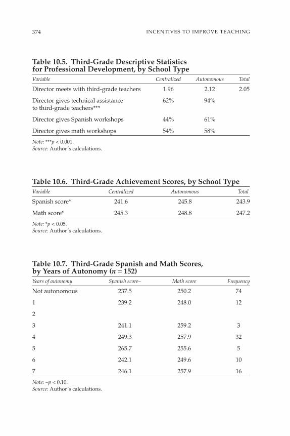
374 INCENTIVES TO IMPROVE TEACHING
Table 10.6. Third-Grade Achievement Scores, by School TypeVariable Centralized Autonomous Total
Spanish score* 241.6 245.8 243.9
Math score* 245.3 248.8 247.2
Note: *p < 0.05.Source: Author’s calculations.
Table 10.7. Third-Grade Spanish and Math Scores, by Years of Autonomy (n = 152)Years of autonomy Spanish score∼ Math score Frequency
Not autonomous 237.5 250.2 74
1 239.2 248.0 12
2
3 241.1 259.2 3
4 249.3 257.9 32
5 265.7 255.6 5
6 242.1 249.6 10
7 246.1 257.9 16
Note: ∼p < 0.10.Source: Author’s calculations.
Table 10.5. Third-Grade Descriptive Statistics for Professional Development, by School TypeVariable Centralized Autonomous Total
Director meets with third-grade teachers 1.96 2.12 2.05
Director gives technical assistance 62% 94%to third-grade teachers***
Director gives Spanish workshops 44% 61%
Director gives math workshops 54% 58%
Note: ***p < 0.001.Source: Author’s calculations.

statistical analysis attempts to provide a model for better understandingwhich of the characteristics contribute to the differences in scores betweencentralized and autonomous schools.
Sixth-Grade Descriptive Statistics
The sixth-grade study covers 145 schools: 52 percent autonomous and 48 percent centralized. Of the sections, 62 percent meet in the morning and38 percent in the afternoon. Among the directors, 64 percent reported usingmultigrade classrooms. Among the schools, 68 percent are in rural areasand 32 percent are in urban areas. In the sample, 53 percent are girls and47 percent are boys.
Control VariablesTable 10.8 shows the student, classroom, and school variables that are con-trolled for in this study. Sixth-grade students resemble third-grade studentsin many ways. Teachers have similar years of teaching experience and edu-
375TEACHER INCENTIVES AND STUDENT ACHIEVEMENT
Table 10.8. Control Variables: Sixth-Grade Mean Values, by School TypeVariable Centralized Autonomous Total
Student characteristics:
Student age 12.84 12.74 12.78
Student SES*** −0.226 −0.111 −0.156
Classroom characteristics:
Classroom mean SES* −0.467 −0.289 −0.369
Mean student age 13.1 12.9 12.99
Mean class size*** 26.0 33.5 30.0
Teaching experience 12.91 13.64 13.31
Total years education 12.9 12.9 12.9
Number of students repeating this year 0.739 0.64 0.684
Students absent this week** 3.03 5.53 4.44
Students absent today** 1.67 4.44 3.22
School characteristics:
Total students 343.4 486.6 417.3
Notes: *p < 0.05, **p < 0.01, ***p < 0.001.Source: Author’s calculations.

cation, and differences between autonomous and centralized schools aresimilar.
Sixth-grade students in autonomous schools are slightly younger thanthose in centralized schools, but the difference is not significant. On aver-age, students in autonomous schools are wealthier than those in central-ized schools (p < 0.001). Mean classroom socioeconomic status differssignificantly by school type. Class size in autonomous schools is signifi-cantly larger than in centralized schools. Autonomous schools have higherlevels of student absence. No significant differences exist in teaching expe-rience or educational levels by school type. Table 10.9 describes schoolsby years of autonomy.
Question VariablesIncentivesAs for third grade, significant differences in incentives exist betweenautonomous and centralized schools. Both teachers and directors in auton-
376 INCENTIVES TO IMPROVE TEACHING
Table 10.9. Years of School Autonomy, Sixth GradeYears of autonomy Frequency Percentage
Not autonomous 69 47.59
1 15 10.34
2 1 0.69
3 2 1.38
4 31 21.38
5 3 2.07
6 9 6.21
7 15 10.34
Total 145 100
Source: Author’s calculations.
Table 10.10. Sixth-Grade Descriptive Statistics for Incentive VariablesVariable Centralized Autonomous
Teacher reports financial incentive*** 27% 64%
Director reports teacher financial incentive*** 38% 87%
Note: ***p < 0.001.Source: Author’s calculations.

omous schools report higher levels of incentives than do those in central-ized schools. Whereas 87 percent of directors in autonomous schools reportthat teachers get financial incentives, only 64 percent of teachers reportreceiving incentives (table 10.10), an even greater gap than in third grade.
ResourcesAs seen in table 10.11, teachers in autonomous schools report significantlybetter school conditions than do teachers in centralized schools. No signif-icant differences exist in the supply of curriculum standards and guides,although slightly more autonomous schools have both standards andguides.
Professional developmentAs with third grade, more professional development is reported in auton-omous than in centralized schools, although only the levels of technicalassistance from the director reach significance (table 10.12).
377TEACHER INCENTIVES AND STUDENT ACHIEVEMENT
Table 10.11. Sixth-Grade Descriptive Statistics for Infrastructure/Material Resources, by School TypeResource Centralized Autonomous Total
School condition according to teacher** 2.099 2.599 2.325
Years implementing standards 2.0 1.86 1.92
Has copy of curriculum standards 71% 81%
Has copy of curriculum guides 89% 91%
Note: **p < 0.01.Source: Authors’ calculations.
Table 10.12. Sixth-Grade Descriptive Statistics for Professional Development, by School TypeVariable Centralized Autonomous Total
Director meets with sixth-grade teachers 1.86 1.93 1.9
Director gives technical assistance 76% 90%to sixth-grade teachers*
Director gives Spanish workshops 37% 46%
Director gives math workshops 38% 51%
Note: *p < 0.05.Source: Authors’ calculations.

Outcome VariablesIndividual math scores are higher in centralized schools (not significant),while no significant difference exists in Spanish scores (table 10.13). Nosignificant difference in scores exists by years of autonomy (table 10.14).
Results
Third-Grade Results
The research question asks whether student outcomes differ by school typeand which teacher or school characteristics are associated with those stu-dent outcomes. Multilevel models were built using student- and teacher-level variables. Table 10.15 shows the multilevel models for third-gradeSpanish (appendix 10.A provides an expanded version of table 10.15).
When looking only at the difference between autonomous and central-ized schools, one finds that autonomous schools, on average, score almostseven points higher on the third-grade Spanish assessment. However,when one controls student characteristics and the role of technical assis-
378 INCENTIVES TO IMPROVE TEACHING
Table 10.13. Sixth-Grade Achievement Scores, by School TypeVariable Centralized Autonomous Total
Spanish score 241.9 242.2 242.1
Math score 248.0 245.5 246.5
Note: *p < 0.05.Source: Authors’ calculations.
Table 10.14. Spanish and Math Scores, by Years of Autonomy (n = 152)Years of autonomy Spanish score Math score Frequency
Not autonomous 237.6 247.0 95
1 232.7 244.4 18
2 237.6 210.1 1
3 239.0 249.0 4
4 238.7 248.7 42
5 233.2 226.9 5
6 236.1 249.3 14
7 245.4 245.3 33
Source: Authors’ calculations.

tance, the coefficient drops to under five points and is no longer significant.As would be expected, student-level variables contributed to the final mod-els. Student age and socioeconomic status are significantly associated withSpanish scores. In addition, girls, on average, score higher than boys. Inter-estingly, when directors give technical assistance, students score, on aver-age, 15 points higher. This finding indicates an important role for onsiteprofessional development in both centralized and autonomous schools.
The fixed-effects model describes the overall difference in scores betweenteachers. The scores do differ significantly by teacher, but the R2 is 0.17,meaning that the model explains only 17 percent of the variation betweenteachers. This finding indicates that the variables used in the statisticalanalyses do not explain a large portion of the variation in scores betweenteachers.135 Table 10.16 shows the multilevel modeling for mathematics.
On average, students in autonomous schools scored 3.9 points higheron mathematics than did students in centralized schools (not signifi-cant).136 Like Spanish scores, mathematics scores are highly dependenton student characteristics. However, whereas girls score significantlyhigher than boys in the Spanish model, gender does not have a significanteffect in mathematics. Similarly, socioeconomic status is not a significantpredictor of mathematics outcomes. In contrast, age is a strong predictor of
379TEACHER INCENTIVES AND STUDENT ACHIEVEMENT
Table 10.15. Third-Grade Spanish AchievementVariable Intercept only Autonomous only Final model Fixed effects
Student SES 5.224*** 4.617**
Student age 3.205*** 3.133***
Student gender −5.754*** −5.238**
School is autonomous 6.914* 4.576 Dropped
Director gives technical 14.589** Droppedassistance to teachers
Constant 242.6*** 239.0*** 201.3*** 217.3***
R2 n.a. n.a. n.a. 0.1657
Log likelihood −16,021.8 −16,019.9 −14,638.2 n.a.
n.a. = not applicableNote: *p < 0.05, **p < 0.01, ***p < 0.001.Source: Author’s calculations.
135. The final model was chosen after testing a large number of student-, teacher-, andschool-level variables. This model had the greatest explanatory power.
136. Although this variable is significant in a simple regression model, it is not in themultilevel.

math scores. Older students tend to have higher math scores than youngerstudents (p < 0.0001). The only classroom characteristic that contributes tothird-grade math scores is the teacher’s years of education, and it is nega-tively associated with math scores. Students, on average, have lower mathscores in classrooms where their teachers have more education.
The fixed-effects model in mathematics is similar to that in Spanish. Themodel has an R2 of 0.15. A significant difference exists in scores by teacheracross the sample, but the model predicts only 15 percent of that difference.
Propensity Score MatchingTable 10.17 shows four different ways of calculating the mean difference inthird-grade Spanish and math scores. The calculated mean difference in
380 INCENTIVES TO IMPROVE TEACHING
Table 10.16. Third-Grade Mathematics AchievementVariable Intercept only Autonomous only Final model Fixed effects
Student SES 1.5 2.6∼
Student age 3.01*** 2.6***
School is autonomous 3.87 3.9 Dropped
Teacher years of −1.9** Droppededucation
Constant 250.5*** 248.5*** 242.2*** 222.1***
R2 n.a. n.a. n.a. 0.15
Log likelihood −17,491.6 −17,491.2 −17,073.5 n.a.
n.a. = not applicable.Note: ∼p < 0.10, **p < 0.01, ***p < 0.001.Source: Author’s calculations.
Table 10.17. Third-Grade Mean Difference in Scores betweenAutonomous and Centralized Schools, by ProcessVariable Spanish Math
Multilevel with no variables 6.9* 3.9
Full multilevel model 4.6 3.9
Stratification matching 2.8 3.9(1.5)∼ (2.1)*
Nearest-neighbor matching 1.8 (0.7) 3.8 (1.4)∼
Note: ∼p < 0.10, *p < 0.05; t-statistics are in parentheses.Source: Author’s calculations.

Spanish ranges from 1.8 to 4.6, depending on the method used. Withpropensity score matching, the average mean difference is smaller than inthe multilevel model, indicating that the process has helped to resolvesome of the selection bias problem. In contrast, there is almost no rangeof mean differences (3.8 to 3.9) in mathematics. Yet, in the propensity score,matching the mean difference does reach significance. From this finding,we can conclude that no significant difference exists between autonomousand centralized schools in third-grade Spanish, whereas there is a signifi-cant and positive effect of autonomy on third-grade mathematics.
Sixth-Grade Results
The sixth-grade results differ from the third-grade results (tables 10.18–10.20).For the sixth-grade Spanish scores (table 10.18), the final multilevel modelshows that students in autonomous schools, on average, score betweenone and two points lower than students in centralized schools (this dif-ference does not reach significance). The only school variable that reachessignificance is the presence of curriculum guides (which was not signifi-cantly different by school type). On average, girls score better than boys,and younger students score better than older students. The fixed-effectsmodel gives us an R2 of 0.23, indicating that student characteristics of ageand gender explain 23 percent of the differences in scores by teacher.
381TEACHER INCENTIVES AND STUDENT ACHIEVEMENT
Table 10.18. Sixth-Grade Spanish AchievementIntercept Autonomous Final Fixed
Variable only only model effects
Student SES 1.9* 1.2
Student age −3.9*** −4.0***
Student gender −9.3*** −9.3***
Classroom mean age −7.7*** Dropped
School has curriculum guides 11.4* Dropped
School is autonomous 1.05 −1.59 Dropped
Constant 239.4*** 238.8*** 385.3*** 197.3***
R2 n.a. n.a. n.a. 0.23
Log likelihood −28,959.8 −28,959.7 −28,844.0 n.a.
n.a. = not applicable.Note: *p < 0.5, ***p < 0.001.Source: Author’s calculations.
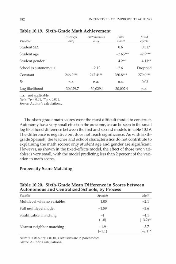
The sixth-grade math scores were the most difficult model to construct.Autonomy has a very small effect on the outcome, as can be seen in the smalllog likelihood difference between the first and second models in table 10.19.The difference is negative but does not reach significance. As with sixth-grade Spanish, the teacher and school characteristics do not contribute toexplaining the math scores; only student age and gender are significant.However, as shown in the fixed-effects model, the effect of those two vari-ables is very small, with the model predicting less than 2 percent of the vari-ation in math scores.
Propensity Score Matching
382 INCENTIVES TO IMPROVE TEACHING
Table 10.19. Sixth-Grade Math AchievementIntercept Autonomous Final Fixed
Variable only only model effects
Student SES 0.6 0.317
Student age −2.65*** −2.7***
Student gender 4.2** 4.13**
School is autonomous −2.12 −2.6 Dropped
Constant 246.2*** 247.4*** 280.8*** 279.0***
R2 n.a. n.a. n.a. 0.02
Log likelihood −30,029.7 −30,029.4 −30,002.9 n.a.
n.a. = not applicable.Note: **p < 0.01, ***p < 0.001.Source: Author’s calculations.
Table 10.20. Sixth-Grade Mean Difference in Scores betweenAutonomous and Centralized Schools, by ProcessVariable Spanish Math
Multilevel with no variables 1.05 −2.1
Full multilevel model −1.59 −2.6
Stratification matching −1 −4.1(−.8) (−3.2)**
Nearest-neighbor matching −1.9 −3.7(−1.1) (−2.1)*
Note: *p < 0.05, **p < 0.001; t-statistics are in parentheses.Source: Author’s calculations.

As for the third grade, propensity score matching was used to addressthe issues of sample selection bias. In Spanish, the mean difference inscores is negative and does not reach significance. In contrast, using pro-pensity score matching, the mean difference in math scores is both nega-tive and significant. Students in autonomous schools, on average, havemathematics scores that are 3.7 to 4.1 points lower than students in cen-tralized schools.
Conclusions
This study has not drawn a neat line between the process of decentraliza-tion, teacher change, and student achievement. It has shown that auton-omous schools look different from centralized schools, particularly interms of financial incentives, school resources, and professional develop-ment. In both third and sixth grades, autonomous schools are more likelyto give financial incentives to teachers, schools have better resources andinfrastructure, and teachers are more likely to receive direct technical assis-tance from the school director. In third grade, autonomous schools are alsomore likely to have curriculum materials. Class sizes, on average, arelarger in autonomous schools. Autonomous and centralized schools dif-fer in their student bodies as well. On average, both third- and sixth-gradestudents are wealthier in autonomous schools, and students are youngerin autonomous schools.
This study has not shown, however, that those differences are linkedto student outcomes. Multilevel modeling and propensity score matchinghave been used to better understand the differences between autonomousand centralized schools and the effect of those differences on Spanish andmathematics outcomes in third and sixth grades. Of the school and teachercharacteristics that are more common in autonomous schools, only thepresence of direct technical assistance contributes to Spanish scores andonly in third-grade Spanish. Spanish scores are positively affected by tech-nical assistance in third grade and by the presence of curriculum guidesin sixth grade. These variables are not unique to autonomous schools,however. In neither third- nor sixth-grade Spanish was a treatment effectfound for autonomy. In contrast, there is a treatment effect for autonomyin mathematics (positive in third grade and negative in sixth grade), butnone of the teacher or school variables in the study contributed signifi-cantly to that difference.
Third-grade mathematics scores are not significantly affected by anytype of teacher and school characteristics identified in this study. Interest-ingly, however, the propensity score matching process indicates that thereis a positive and significant autonomy effect on the third-grade mathe-matics score of almost four points. Third-grade students in autonomousschools have higher average math scores than students in centralized
383TEACHER INCENTIVES AND STUDENT ACHIEVEMENT
schools, but the teacher and school characteristics in this study do not con-tribute to that difference. In sixth-grade mathematics, although there is asignificant difference in average scores by school type (students in auton-omous schools score 3.7 to 4.1 points lower than those in centralizedschools), the model does not explain enough of the variation to haveexplanatory power. Although math scores were found to be higher inautonomous schools in third grade, they are lower in autonomous schoolsin sixth grade. This negative autonomy effect at higher levels deserves fur-ther investigation.
Although this study contributes to a better understanding of incentives,infrastructure, and professional development in autonomous schools com-pared to centralized schools, it has not shown clear differences in out-comes between centralized and autonomous schools. An initial hypothesisof this chapter was that the effects of decentralization contribute tochanges in teacher behavior, with resultant changes in student outcomes.This study has not shown a clear relationship between the three.
In the Nicaraguan context, as described earlier in this chapter, decen-tralization takes many forms and is implemented in many different ways.A recent study of Nicaraguan autonomy found vastly different views ofboth the effects of autonomy and the definition of autonomy itself, indi-cating that there may be more differences between autonomous schoolsthan between autonomous and centralized schools (Asencio and others2001). Teachers no longer are assured of having school-based financialincentives. That factor may limit the role incentives play in producingchange (in contrast, the World Bank–funded incentive tied to class size ismore stable, and class sizes in autonomous schools are significantly higherthan those in centralized schools). When incentives are unstable and donot depend on teacher behavior, it can be hypothesized that their effecton teacher behavior—and thus on student outcomes—is limited.
This study provides a context for future research on student achieve-ment in Nicaragua. As more and more schools adopt the governance struc-tures of autonomous schools (by law, all schools will be decentralized by2006), it will become more imperative to continue to identify which aspectsof school autonomy contribute to positive student outcomes. Onsite pro-fessional development by the school director appears to be one importantvariable, as does the availability of curriculum resources. If financial incen-tives for teachers become more stable and more clearly linked to teacherbehaviors, they may also contribute to student outcomes. Those variablesappear to have different effects on Spanish than on mathematics, however,and this finding deserves further investigation. Finally, given the differ-ence in autonomy effects for third and sixth grade, longitudinal researchwill provide important information to better understand the learningexperience of students across various grade levels.
384 INCENTIVES TO IMPROVE TEACHING
References
Arcia, G., and H. Belli. 2001. La autonomía escolar en Nicaragua: Reestable-ciendo el contrato social. Managua: PREAL.
Arnove, R. F. 1995. “Education as Contested Terrain in Nicaragua.” Com-parative Education Review 39(1): 28–53.
Asencio Florez, C., R. Ruiz Carrión, V. Sequiera Calero, V. Castro, andA. Gershberg. 2001. Lecciones aprendidas de la autonomía escolarNicaragüense. New York: New School University.
Castillo, M. 1998. “La descentralización de los servicios de educación enNicaragua.” Serie Reformas de Política Pública. Naciones UnidasComisión Económica para América Latina y el Caribe, Santiago.
di Gropello, E. 1997. Descentralización de la educación en América Latina: Unanálisis comparativo. Santiago: CEPAL.
di Gropello, E., and R. Cominetti, eds. 1998. La descentralización de la edu-cación y la salud: Un análisis comparativo de la experiencia Latinoameri-cana. Santiago: Naciones Unidas.
Fuller, B., and M. Rivarola. 1998. “Nicaragua’s Experiment to DecentralizeSchools: Views of Parents, Teachers and Directors.” Working Paper onImpact Evaluation of Education Reforms 5. World Bank, Washington,D.C.
Gershberg, A. I. 1999a. “Decentralization, Citizen Participation, and theRole of the State.” Latin American Perspectives 26(4): 8–38.
———. 1999b. “Fostering Effective Parental Participation in Education:Lessons from a Comparison of Reform Processes in Nicaragua andMexico.” World Development 27(4): 753–71.
———. 2003. “Empowering Parents While Making Them Pay: Auto-nomous Schools and Education Reform Processes in Nicaragua.”Paper written for the project Empowering Parents While Making
385

Them Pay: Autonomous Schools in Nicaragua, funded by the TinkerFoundation, New York.
Gershberg, A. I., and B. Meade. 2003. “Parental Contributions and School-Level Finances: An Analysis of Nicaraguan Autonomous School Bud-gets.” Paper written for the project Empowering Parents While MakingThem Pay: Autonomous Schools in Nicaragua, funded by the TinkerFoundation, New York.
Gershberg, A. I., and D. Winkler. 2000. Education Decentralization in LatinAmerica: A Review of the Effects on the Quality of Schooling. In S. J.Burki, ed., Decentralization and Accountability of the Public Sector: Pro-ceedings of the 1999 Annual World Bank Conference on Development in LatinAmerica. Washington, D.C.: World Bank.
Kaestner, R., and A. I. Gershberg. 2002. “Lessons Learned from Nicaragua’sSchool Autonomy Reform: A Review of Research by the NicaraguaReform Evaluation Team of the World Bank.” Paper written for the proj-ect Empowering Parents While Making Them Pay: Autonomous Schoolsin Nicaragua, funded by the Tinker Foundation, New York.
King, E. 1996. Nicaragua’s School Autonomy Reform: A First Look. Washington,D.C.: World Bank.
King, E., and B. Ozler. 2000. “What’s Decentralization Got to Do withLearning? The Case of Nicaragua’s School Autonomy Reform.” Work-ing Paper Series on Impact Evaluation of Education Reforms. WorldBank Development Research Group, Washington, D.C.
King, E., B. Ozler, and L. Rawlings. 2000. Nicaragua’s School AutonomyReform: Fact or Fiction? Washington, D.C.: World Bank.
MECD (Ministry of Education, Culture, and Sports). 2003a. “Evaluacióndel rendimiento académico de los estudiantes del 3ro y 6to grados deprimaria: Informe de resultados 2002.” Managua.
———. 2003b “Estado de la formación de la ciudadanía y recursoshumanos: La educación en Cifras.” Managua.
———. 2003c. “Ministry of Education Data.” Ministry of Education,Department of Statistics, Managua.
———. 2004. “Autonomía Escolar.” Managua. http://www.mecd.gob.ni/autonom.asp. Accessed April 4, 2004.
386 INCENTIVES TO IMPROVE TEACHING

MIGOB (Ministry of Government). 2003. “National Development PlanProposal.” Government of Nicaragua, Managua.
Morales, A. 2002. “Colegios tendrán más fondos por menos alumnos.” LaPrensa (Managua), July 24, p. 3.
Tedesco, J. C., and N. López. 2002. “Desafíos a la educación secundaria enAmérica Latina.” Revista de la CEPAL 76: 55–69.
387TEACHER INCENTIVES AND STUDENT ACHIEVEMENT


11Political Economy, Incentives,
and Teachers’ UnionsCase Studies in Chile and Peru
Luis CrouchResearch Triangle Institute
The unionization of teachers and collective bargaining [is] likely tocontribute to increasing rationalization. Unions will seek new rulesand procedural safeguards, and management will counter with newrules and procedures of its own. . . . Major losers [in the struggle forpower] will be teachers who will see their professional autonomyreplaced by a bureaucratic conception of their role. The most tragicloss will be to the students who are cast as objects being prepared toassume their place in society.
—A. Wise
As other chapters in this volume show, in the past decade or so manycountries in Latin America have introduced various incentive or incentive-like mechanisms to stimulate more, or better-directed, teacher effort andaccountability. Those mechanisms range from formal incentive systems,such as some version of pay-for-performance (as in Chile), to informal orgeneralized incentives, such as those involved in community-basedaccountability (as in El Salvador or Honduras). Other chapters assess theeffectiveness of the various incentives approaches using evaluationmethodologies.
Instead, this chapter addresses issues related to the political economy ofchanges in teacher incentives regimes. What has made it possible to intro-duce and implement changes in incentives in some countries? What rolehave unions for teachers played in determining the nature and types ofincentives that might be acceptable? What features of teacher unionism, orof the economics and political economy of incentives, have led to opposi-tion in some cases and support in others? Most important, what lessons—
389
The epigraph to this chapter is drawn from Wise (1979, pp. 200 and 212).

either from the case studies, from other international experience, or frombasic principles—can be learned for increasing support to teacher-incentivereforms in the future?
The chapter is based on some understanding and modeling of first prin-ciples from the literature and on two case studies: Chile and Peru. The casestudies show quite different outcomes: Chile has managed to not onlydesign but also implement incentives systems, whereas Peru has beenmuch less successful with detailed, practical, and consistent (and, hence,implementable) design and implementation.
Because the chapter is based on only two cases, it does not propose easygeneralizability of the lessons that emerge nor does it even pretend to testhypotheses. However, because the cases illustrate principles that appearfairly strong, some degree of generalizability should exist, at least withrespect to the sorts of issues that should be considered as countries pro-ceed to design or refine incentives systems. Valid pointers for how to pro-ceed and how to think about the issues do emerge from the cases and fromfirst principles, even if lessons about “what works” are less strong.137 Theintent of the chapter is not so much to provide generalizable lessons or totest hypotheses, as to point toward agendas for further analysis. Aftersufficient hypotheses are formulated, continentwide studies of the role ofunionism might be feasible.
The chapter uses a document review and key-informant interviews.No primary data gathering or secondary data analysis was carried out.
Case Study of Chile: Reforms Designed and Implemented, Effect Yet to Be Seen
In the 1980s and 1990s, Chile has introduced some of the most extensiveaccountability and accountability-based incentive systems among middle-income countries—perhaps even among high-income countries. Someaspects of those systems and approaches were started, albeit in crudeform, under the military government (1973–90), but serious educationreforms started in 1980. A subset of those systems was continued under thedemocratic governments since 1990, but the democratic governments haveadded more sophistication to the accountability and incentive systems.
Many of the systems introduced after democratization began after con-sultation and negotiations with civil society, in particular with the teachers’union (the Colegio de Profesores de Chile, or CP). In some cases, particu-larly early in the democratization process, the consultations were fairly
390 INCENTIVES TO IMPROVE TEACHING
137. Thus, generalizing good process and good use of basic principles related to unionsand incentives is probably safe. Simply copying to other places the incentives that may haveworked in one place, or may look as if they will work in one place, is probably not safe.

minimalist. More recently, consultations have become extensive and have,in fact, become co-design.138 The reforms had political implications orrequired political compromises, and those issues were dealt with forth-rightly, especially in recent years. How the compromises were gener-ated is the main theme below. Before turning to this topic, however, threeelements of background information are provided: (a) key elements ofthe reform created by the military government, (b) main aspects of thenature of teachers’ unionism in Chile, and (c) a description of the basicincentives that have been negotiated.
Landscape under the Previous Government
The military government in Chile carried out several fundamental reformsthat are germane to the issue of incentives and accountability:
• Education was “municipalized,” which means public school teachersbecame municipal rather than central government employees, andschools came under municipal management, at least in a formal sense.School principals and municipal mayors were directly appointed by thecentral government. In this sense, the notion of municipalization beingused was a rather peculiar one, and the centralist appointment of schoolprincipals had important consequences for the future.
• Funding was put on a per capita basis, and municipal public schoolsand private schools were put on the same funding basis to generatecompetition between schools within and between types. Funding ofmunicipalities’ educational responsibilities was put on a formula basis,with attendance as a key driver. This reform would also stimulate atten-dance and enrollment. The approach was expected to create a quasi-market in educational services, with built-in incentives for efficiency.139
• To provide market information and to create a metric for quality, whichcould thus inform the choices of parents as consumers of school services,a measurement system for results was created, the PER (Programa deEvaluación del Rendimiento). The logic of this approach was from itsinception to provide accountability data to a market of consumers,rather than to provide suppliers with information on how to improvethe services being offered.
391POLITICAL ECONOMY, INCENTIVES, AND TEACHERS’ UNIONS
138. As in the case of the new Sistema de Evaluación del Desempeño Profesional Docente—an individual, high-stakes, teacher evaluation system with high-incentive implications, not tobe confused with the Sistema Nacional de Evaluación de Desempeño de los EstablecimientosEducacionales (SNED), which confers group rewards.
139. In a sense, the principle is that government “buys” places for children in school,with parents as its agents. Those schools that cannot produce at the price the government iswilling to pay are outcompeted. The efficient survive.

While those reforms were being carried out during the 1980s, however,total spending plus spending per student declined in real terms by about25 percent (González 2003). Total enrollment in the public system or sub-sidized private system was essentially static, and there was some smallgrowth in the private nonsubsidized system. The available data do notallow us to evaluate to what extent there were improvements in learningduring this period.
A Few Key Characteristics of the Chilean Teachers’ Union
Chile’s powerful teachers’ union, the CP, derives its power from a few fac-tors:
• It is a largely monopolistic organization. A few other relatively minorteachers’ associations exist, but the CP encompasses the overwhelm-ing majority of unionized teachers. The CP was created by the militarygovernment in 1974, and constituted as a monopoly to which teachershad to belong, but the situation was liberalized in 1980. As a result, analternative union sprang up, which was in a more traditional mold anddid not owe its existence to a mandate from the government. In unionelections for the CP in 1985, elements more friendly to a traditionalunion style won. The alternative union was disbanded, because, as ofthat election, the CP fulfilled the need for more traditional unionism(see Nuñez Prieto 2003). In an ironic sense, then, the military govern-ment may have been indirectly responsible for the power of this orga-nization.
• The union formally encompasses teachers of all political views. On ascale of 1 to 10, with 1 being “left” and 10 being “right,” teachers self-classify as very centrist or somewhat left-of-center. The average self-classification is 4.9. The current leadership, however, is identified with theCommunist Party (the leadership affiliated with this party won 76 per-cent of the vote in the most recent election for which we have data).Interestingly, however (as will be seen later), since this leadership cameto power, there has been more movement in the direction of individualevaluation with fairly high stakes (see Nuñez Prieto 2003).
• The union’s bureaucratic and technical leadership is of high intellec-tual and organizational caliber. Advisers to the CP and its high-leveltechnical leadership have considerable experience and have publishedscholarly and technical papers on many areas of educational quality. Acasual review of the union’s journal, Docencia, makes it clear that theintellectual level of the magazine is very high. Position notes andspeeches of the CP are considerably more thoughtful than similar uniondocumentation from other countries, and they focus on substantivematters of education policy, not simply on traditional union issues (see
392 INCENTIVES TO IMPROVE TEACHING
Assael Budnik and Urrutia 2002; Pavez Urrutia n.d.; Scherping 2003a,2003b, 2003c; Verdugo 2004).
• The union’s internal organization appears to be increasingly democratic,and its external positions are based on participatory development ofpositions. This trend is particularly seen after 1997, when the CP held itsfirst major congress after the renewal of political democracy in Chile.
• The same 1997 congress induced the leadership, under pressure fromthe rank and file, to take more interest in educational and pedagogicalissues, instead of bargaining and bread-and-butter issues. This shiftled to changes in the internal emphasis of the CP, as well as in its offer-ings to its membership. It led, for example, to the emergence of a formalmovement within the union, the “Movimiento Pedagógico,” aimed atproviding alternative ways of conceptualizing education.
• Both the union and the past-1990 government had been in the opposi-tion during the military government from 1973 to 1990. Furthermore,from 1990 to 1995, the union was controlled by parties in the same polit-ical alliance as the government of the country. This connection wasimportant, because it created an atmosphere of some trust and credi-bility. In the context of imperfect information about intentions that char-acterizes public sector bargaining (because the government is not asimple maximizer of a clear objective function), trust and credibilitytake on great importance.
Changes in Incentive Regimes since 1990
During the 1990s and early 2000s, there were massive increases in spend-ing, in general, as “supply side” incentives, plus many innovations withperformance-based incentives and competitive grants of various sorts.Total spending in the 1990s increased about 180 percent, and per studentspending increased about 130 percent (González 2003). Most important,average teacher compensation increased substantially in real terms, againby about 150 percent in the 1990s (Mizala and Romaguera 2003). In addi-tion to improving salaries, various incentive schemes have been negoti-ated, approved, and implemented. The following incentives stand out inchronological sequence:
• Collective performance-based incentives are related to measured stu-dent achievement. For instance, the Sistema Nacional de Evaluación deDesempeño de los Establecimientos Educacionales (National System ofSchool Performance Assessment, or SNED) was negotiated in the mid-1990s and gives groups of teachers a salary bonus depending on perfor-mance of the whole school on the Sistema de Medición de la Calidad dela Educación (Education Quality Measurement System, or SIMCE) tests.
393POLITICAL ECONOMY, INCENTIVES, AND TEACHERS’ UNIONS
• The Asignación por Excelencia Pedagógica rewards individual teachersbased on process criteria, not learning results. It was negotiated in 2000and initiated in 2002, and teachers submit voluntarily.
• Under Law 19715 of 2001, if teachers are evaluated well in the Asignación por Excelencia Pedagógica, then the Red de Maestros deMaestros, may propose projects so they can mentor other teachers andreceive financial incentives to do so.
• An increase in the size of the reward associated with the SNED wasnegotiated in 2003.
• Creation and approval of a Sistema de Evaluación del Desempeño Pro-fessional Docente, a nonvoluntary system (as opposed to the Asignaciónpor Excelencia Pedagógica, which is voluntary) of performance review,made it possible for teachers to receive individual rewards (AsignaciónVariable por Desempeño Individual) that are based on peer-reviewedteaching ability (rather than student learning achievement). Thisupgraded incentive was negotiated in 2003 and is being applied tothe first set of teachers during 2004. In a sense, it is the fulfillment ofthe obligatory individual performance review system mandated in theEstatuto Docente in the early 1990s, a system that took some 13 yearsto come to fruition.
In addition, many incentives exist that are not linked to performance,such as rurality incentives (or “difficult conditions” incentives) andrewards tied to administrative duties. Finally, there were many othermajor policy changes, such as the gradual elimination of double shifts,changes in how schools are funded (for example, the introduction offees in public secondary schools, or the financiamiento compartido system),competitive school grant schemes, poverty-targeted programs, and curric-ular reforms.
In summary, Chile has managed to design and implement various per-formance incentive mechanisms throughout the 1990s. Some of those mayhave taken a long time and endless rounds of negotiation, but they are areality. Nevertheless, as Mizala and Romaguera (2003) argue, the greatvariety and complexity of the incentives may dilute the messages theysend. Moreover, the incentives may not be having the effect that washoped for because teachers’ ability to respond to the incentives may not besufficiently strong. Such questions are for further empirical research.Nonetheless, the achievements are notable and raise the question as tohow they were accomplished.
Factors Making the Changes Possible
Chile has created a far-ranging mix of individual and small-group incen-tives for teachers, including broad incentives related to overall improve-ments in salaries of teachers. The individual and small-group incentives
394 INCENTIVES TO IMPROVE TEACHING

are not typical of education sectors, especially in developing countries,and are often opposed by teachers’ unions. As noted previously, Chilehas an active and powerful teachers’ union. How then was Chile able to setup such systems? The following reasons stood out in discussions and doc-uments or are offered as original hypotheses in this report.
Leadership in the Ministry of EducationA first factor in explaining breakthroughs on incentives is the level ofleadership in the education sector in Chile. “Leadership matters” is oftentaken by economists as a nonexplanation, or as a rather banal explana-tion, especially when it is implicitly defined circularly as a vague set ofcharacteristics that are of people in formal leadership and that lead toresults. If a good leader is someone who can deliver on reform results,then attributing reform results to good leadership is not very useful. But,in the case of Chile, one can assess the quality of leadership in quite objec-tive terms: For example, in terms of education background and previous(or subsequent) experience in the Ministry of Finance or other high levelsin the social and political structure.
Objectively, then, in terms of education background, four of seven min-isters of education since 1990 have advanced degrees in economics (threePh.Ds., one M.A.), specifically from Harvard and Duke. Another had a Ph.D.in education from Harvard University, but with economics and operationsresearch emphases. Yet another had no advanced degree in economics, butdid have a B.A. in the prestigious Ingeniero Comercial field in Chile. Similarly,in terms of previous or subsequent experience at high levels in Chileansociety, two ministers, including the one who was perhaps the most impor-tant in negotiating the first breakthroughs in the incentives reforms, hadcabinet-level experience in the Finance and Planning Ministries. Anotherwent on to be president. One minister had plied his practical experiencewith public and private management in helping the CP solve internal finan-cial problems, which helped create good relations with the CP.
All of these leadership factors are more or less objective and are notcircularly defined with respect to reform success. The fact that such promi-nent people, who are well-qualified in statecraft, were ministers of educa-tion is likely a partial cause of the breakthroughs in incentives regimes.But the quality among leaders could also be, partly, a manifestation of thefact that government simply took education very seriously, and this gen-eral seriousness was the more-operant cause of breakthroughs than theappointment of very good leadership.
Role of the Ministry of FinanceThe Ministry of Finance took an unusual level of interest in the educationsector—unusual by both worldwide and Latin American standards. Manyof the key reforms, such as the SNED, were initially sketched out in themid-1990s in collaborative, technical sessions between key actors at the
395POLITICAL ECONOMY, INCENTIVES, AND TEACHERS’ UNIONS

Ministry of Finance and at the Ministry of Education. The leadership fromthe Ministry of Finance that was crucial to this redesign then went on tolead the education sector, which may help explain why implementationwas pursued after initial design. It also reaffirms the notion that the gov-ernment tended to put economically minded leadership in the educationsector. High-level formal and informal technical interactions between theMinistries of Finance and Education took place frequently during the mid-1990s. Even though this sort of collaboration put the economists in charge,it also meant that commitments to increase educational funding, whichwere tied to reforms, tended to be more credible.
Role of the UnionThe quality of leadership extended to the CP as well. The CP has adviserswho have worked independently (that is, not as part of their union orpolitical affiliation) in education think-tanks and as consultants and advis-ers to private and nongovernmental organization (NGO) schools. Someof the leadership is involved in important roles in international initia-tives, such as Education International, the Confederation of AmericanEducators (Confederación de Educadores de América, or CEA), andPREAL (Programa de Promoción de la Reforma Educativa en AméricaLatina, or Partnership for Education Revitalization in the Americas—ajoint effort of the Inter-American Development Bank and the Inter-American Dialogue).140 The leadership also has strong credentials inChilean political life, given the members’ background as militants in vari-ous parties in the opposition to the military regime and their decades ofexperience as union leaders. As noted previously, the writing of the lead-ership reflects serious thinking about education policy issues, well beyondtypical union “militancy” issues. This focal point may be partly inresponse to pressure from rank-and-file teachers, but whatever the sourceof this pressure, the leadership has had the capacity to respond.
The high quality of leadership on all sides—the fact that many of theleaders were among the most experienced Chileans in the managementof the state and the fact that so many of them had decades of negotiatingexperience—was a key determinant of the breakthroughs. The lessonappears fairly clear: if education is taken seriously, a good way to show itis to put the most-qualified people in the society in charge of the sector.Whether this positioning would always lead to good results is anotherstory. However, the obverse, namely that good results are unlikely if theleadership is not of high quality, seems a safe conclusion.
The Logic of Collective Action and Generalized Salary Increases
396 INCENTIVES TO IMPROVE TEACHING
140. Information about PREAL can be found on the organization’s Web site, http://www.preal.org/.

The changes toward individual or small-group incentives in Chile tookplace (a) during a period of strong government commitment to general-ized salary increases and (b) when government was delivering on its com-mitment in a way that was clear to all those concerned. Furthermore, thekey breakthrough negotiation on small-group incentives (the SNED) tookplace only as part of a bargaining process that involved other key reforms,such as the possibility of eliminating redundant teacher posts (which theunions opposed), and against the background of generalized salaryincreases (which the unions favored). As reported by Mizala and Roma-guera (2003), by the mid-1990s average and base salaries had alreadyimproved substantially (by at least 70 percent in real terms) since the lowsexperienced during the military government.
Resisting individual incentives until general or base salaries haveimproved has a certain commonsense logic and populist appeal. This fac-tor was clearly operational in the union discourse in Chile, as summarizedby observers (Belleï 2004; Nuñez Prieto 2003). The reality is that by 1990the starting teacher salary was below the poverty line (Belleï 2004). A pre-occupation with equality or equity is not peculiar to unions. In fact, mostmodern institutions (the World Bank, for example) generally favor somedegree of nonmarket solutions to inequality, such as use of tax bases togenerate redistribution through progressive spending incidence orpoverty-targeted programs. The concern with equality is common tomany institutions associated with “modernism,” at least since the late18th century. Although unions are certainly a prime example of this trend,they are hardly unique in this respect.
The resistance to individual incentives also has a much more practicaland instrumental basis in the logic of union action and mobilization. Thatbasis is related to the oft-observed phenomenon that the rank and fileseem to be more accepting of merit pay than union leadership (see Ballouand Podgursky 1993 for an example). Seeking and achieving collectivegoals, such as improvements in base and average pay, requires collectivemobilization. For example, the rank and file must be amenable to go onstrike and not break strikes. Such action requires that the individual highlyidentify with the whole (Brimelow 2003). This collective identification islikely to be undermined if the reward structure emphasizes individualeffort. Then, the returns to individual effort could become higher than thereturns to collective effort, thus reducing incentives for collective effort toseek generalized improvements.141
397POLITICAL ECONOMY, INCENTIVES, AND TEACHERS’ UNIONS
141. In the United States, this sort of reasoning (though not exactly this logic) is anaccepted administrative principle. Brimelow (2003, p. 85) quotes the State Public EmployeesRelations Board of California, which issued the judgment that “The provision of benefits thatare more than what is called for in a collective bargaining agreement is inherently destructiveof a union’s representation rights. It can be construed to give a message that unit employeeswould do better if they abandoned the union.”

It is not the case that any reward to individual effort will make thereturns to individual effort higher than the returns to collective effort.Given free-rider effects in collective efforts, it is clear that even fairly smallreturns to individual effort will tend to undermine the few—essentiallynonmonetary—individual incentives for collective effort that do exist.Note that this is not the same as saying that individual rewards cannotvary or else collective identification is undermined. If individual rewardsvary according to factors unrelated to individual effort, such as seniority,preservice training, or differential cost of living in certain areas, then theability to make individuals identify with the collective group, so that theywill press for overall improvements, is not undermined.
As a result, when collective goals, such as improvements in averagepay, are seen as legitimate by the rank and file (for example, because basestarting salaries for teachers are below the poverty line), then the rankand file may identify with the leadership’s positions against pay for indi-vidual effort. A negative interpretation is that union leadership will findit easier to manipulate and control the rank and file—for self-seekingpurposes—if the rank and file are all equal. Although this interpretationmay be true in some unions, it need not be the case for the logic laid outhere to be operational. The rank and file may well understand the implicitneed for sameness in generating solidarity.
Simpler propositions suggest opposition to individualized incentives toeffort and are based on median-voter analyses. For example, (a) if the indi-vidual teacher is risk-averse and does not know where he or she would fallin the distribution of ability to generate results in measured studentachievement, and (b) if the increase in performance-related pay comes atthe expense of existing generalized improvements (that is, if performance-related pay is seen as a redistribution of existing average pay, or as analternative to a one-time increase in average pay), then the median voter inthe rank and file would tend to oppose the introduction of performance-related pay. However, it is unlikely in the long run that this process wouldbe a strong determinant if generalized increases are taking place at the sametime the performance-related pay is introduced. Therefore, performance-related pay would not be seen as a zero-sum game. Individual rewardsundermine collective effort even when average salaries are going up,whereas even a risk-averse individual might not be as opposed to indi-vidual rewards if the rewards were not a zero-sum game. Thus, if the realincentive or perceived need for collective mobilization is high, teacherswill tend to oppose rewards for results that are based on individual effort.
398 INCENTIVES TO IMPROVE TEACHING
142. Union leadership, at least where it has been studied, is not any more crudely self-serving than political leadership in any other area of democratic life in particular countrycontexts—see Freeman and Medoff (1984).

Furthermore, as later discussion of union behavior will show, median-voter propositions do not fully explain union leadership behavior, evenwhere unions are highly democratic and the leadership is not self-serving.142
For example, rank-and-file teachers are often not opposed, in principle, toperformance-related pay (see Ballou and Podgursky 1993; specificallyfor Chile, see Mizala and Romaguera 2003; for Peru, see Ministerio deEducación/IIPE-UNESCO 2002). Similarly, some evidence suggests thatunion leadership engages in more political activity and political activityof a different sort than the rank and file might want. Incidentally, unionleaders may be more successful at the political activities they see as impor-tant than at the ones the rank and file might see as important (see Mastersand Delaney 1987; Freeman and Medoff 1984). Instead, a “managerialist”approach to unions (Pemberton 1988)—where the dynamics between theleadership and the rank and file are assumed to be more complex thanmedian-voter models suggest—might propose that the rank and file“delegate” any opposition to performance-based pay to the leadership.Such delegation would be a way of generating the solidarity needed tofight collectively for better average pay when seeking average increasesis important to the rank and file and when winning such struggles seemspossible. In fact, some analysts or commentators who have the deepestinsider knowledge of unions, such as Lieberman (2000), place most of theburden for an explanation of why unions are opposed to most reforms ona managerialist rather than median-voter view of teacher unions. Thoseanalysts observe that, where reforms such as vouchers or increasedaccountability to parents are seen as reducing the hold of union leadershipon the rank and file, the reforms threaten access of the leadership to mem-bership dues and the strike tool.143
In summary, because general salaries were increasing in Chile duringthe 1990s, individual teachers would not have to worry about an absolutedecline in salary if they were found to be poor performers, and alsobecause of the increase in general salaries, the need for collective alle-giance to a fight for general salary improvements perhaps declined. Forboth reasons, in the case of Chile, improvements in general pay that wereseen as likely to continue (because they were credible) probably favoredbreakthroughs in individualized or small-group incentives.
An important implication of Chile’s experience is that, because indefinitegeneralized improvements in average pay are not likely in most countriesbut are probably available only during periods of catch-up, educationsector leadership should take advantage of such periods to overcome thelogical—and in many ways justified (in practical terms, if not necessar-
399POLITICAL ECONOMY, INCENTIVES, AND TEACHERS’ UNIONS
143. Although these sorts of points of view are associated with critics of the unions, suchas Brimelow (2003) and Lieberman (2000), there is no inherent reason why a more nuanced orneutral point of view, such as Moore (1976), who also attempts to explain uniformity inwages, should not prefer a managerialist viewpoint.

ily in terms of ultimate justice)—resistance of teachers and unions toperformance-related pay when average salaries are perceived to be too low.
Social Accountability Pressure
As will be seen, in spite of dramatic increases in salaries and spending inthe 1990s, results have not kept pace. Results of education reforms can takea long time to show up in achievement statistics or other indicators ofobjective results, and signs for the future are encouraging. It is also likelythat the speed of quality response can be improved in Chile to shortenthe gestation period of quality response to the reforms. But, for now, thepoint to be noted is that the media, civil society organizations, and general public opinion—not to mention finance ministers, cabinet, andlegislatures—are unlikely to fully heed the gestation-period argumentand to be as patient with reforms as educators would like them to be. Theimpatience of policymakers was already becoming evident in the mid-1990s and gained strength in the late 1990s. For that reason and becauseaverage pay was already increasing, it would have been less-and-less ten-able for the CP to argue that there should not be some form of account-ability for teachers. Their future as a professional organization willing totake accountability for the quality of education—as opposed to simplebread-and-butter issues—and their ability to speak collectively for teach-ers as professionals would have been undermined by a stance that refusedto associate the results of the sector with individual or small-group workeffort and creativity. In most other occupations considered to be “profes-sional,” considerable relationship exists between reward and individualeffort, as well as considerable direct connection between professionalworker and client. Thus, disassociating the union and teachers from thisaccountability pressure would have tended to undermine the union’sstance that teachers should be treated as professionals.
Nevertheless, logic operates in most countries, even developing coun-tries. Thus, this explanation cannot help us understand why that logic sup-ported change in Chile, where two special circumstances had to be takeninto account. First, much had already been done in terms of access to edu-cation. Certainly, by the early 1990s, a preoccupation with quality andachievement had set in. Clearly, quality improvements, as opposed toaccess improvements, require more work (or different work) from teach-ers. Second, in Chile as opposed to many other countries, recurrent report-ing (at least to the government, later on to the public) of schooling results
400 INCENTIVES TO IMPROVE TEACHING
144. It is important to note, however, that though the intertemporal comparability of theSIMCE results was, at best, suspect until the tests were improved in the late 1990s, the generalpublic and opinion-makers were generally relatively immune to subtleties of this nature.

on a fairly objective basis was already common in the early 1990s and cer-tainly by the mid-1990s. Furthermore, Chile participates willingly in inter-national assessments, which are widely discussed in the media.144
Therefore, the public and opinion-makers find it relatively easy to seewhether results are improving at a pace that they believe is commensuratewith spending increases and with improvements in teachers’ conditions.This availability of information may lead to an impatience that is some-what unjustified, again because in education there is a long lag betweenspending and results and because the sector was recovering from very lowspending levels in the late 1980s. But, justified or not, the data availabilityand the public debate atmosphere that reigns in Chile certainly put pres-sure on both unions and the ministry to look for ways to create linksbetween improvements in pay and results delivered, which, in turn, ledto a serious consideration of individual or small-group incentives.
Attributability of Collective Results and Individual Process
Chile’s incentives regime effectively tries to address key attributabilityproblems. To explain why and how requires some digression.
Agency theory predicts that incentives matter most (a) if they aredirected at actual results rather than at precursor processes or behaviors,and (b) if the results are relatively easily attributable to the agents enjoyingthe incentives.145 The attributability aspect applies in two ways. First, theincentives have to apply to the set of agents that will create the results. Sec-ond, the agents have to actually be able to affect the results and have tobe largely the only ones affecting the results. Those observations have twoimplications: first, to the degree that the results are generated collectively,the incentives have to be collective. Second, to the degree that one isencouraging results beyond the easily measurable ones and to the degreethat one does not have an exact model of how each type of behavior leadsto each type of result, then individual or group incentives have to focuson processes and precursors rather than on final results. Markets rewardcomplex goods largely in this way. The price one pays for the experience ofdining in a fine restaurant is not decomposable into rewards for easilymeasurable “components” of the dining experience. Thus, the problemarises when a bureaucracy tries to create bureaucratically driven incen-tives for results, but the incentives cannot be complex and general (theway the price of a meal in a fine restaurant is), because they have to betransparent and must yield to public accountability, and because the pro-ducer has no strong incentive to take prices into account and to put effortinto assessing how to get the best price using complex trial-and-error
401POLITICAL ECONOMY, INCENTIVES, AND TEACHERS’ UNIONS
145. For a thoughtful review of agency theory, see Prendergast (1999).

methods, the way that, say, restaurant owners do. However, in the case ofcollective incentives, there is always a free-rider problem that is difficult tosolve if the group is so large that free-riding is difficult to detect. If thegroup is too large, then incentives are unlikely to work well. Table 11.1summarizes.146
The interesting cases are in the diagonal that goes from lower left toupper right in table 11.1. The upper-left-to-lower-right diagonal definesthe ambit of pure market incentives or pure group loyalty (forced or spon-taneous) and bureaucratic rules as opposed to incentives. Thus, this otherdiagonal is less relevant to the case at hand.
The more that process incentives (lower left-hand corner in table 11.1)are informed by sound professional judgment of direct practitioners (ifthey have an incentive to keep up the image of the profession), the better.Such direct practitioners, as opposed to bureaucratic managers, often havethe most-subtle information on the precise precursor behaviors that willlead to the broader results. This is why codes of conduct that are deter-mined by and enforced through professional associations can work—aslong as the association has a real incentive to maintain its image and haseffective sanction mechanisms to control the behavior of individuals whowould free-ride on the image of the profession.147 Peer-based evaluationsin merit-pay systems have, therefore, been proposed and tried, althoughhow well they really work is still debatable (see Brimelow 2003; Kerchner,Koppich, and Weeres 1997, 1998; Lieberman 2000).
The development of education incentives in Chile seems to wisely takeinto account the sorts of issues discussed above. This taking into accountwas partly determined by the technical ability of designers in the min-istry and the CP, partly caused by bargaining by the CP in the design ofincentives regimes, and, surely, partly caused by good luck.148 The fact thatbargaining and a sequence of reaction and counter-reaction played somerole is evidenced in the original Estatuto Docente, which was crafted in1991 and which called for individual evaluations that were not imple-mented because of teacher opposition. Teachers were against the notionof an evaluation system that did not involve their input in either design
402 INCENTIVES TO IMPROVE TEACHING
146. Note that these arguments do not define the issues as public or private goods. Thearguments are about the nature of production by public or private bureaucracies, similar tothe logic regarding the optimality of outsourcing. But the logic of excludability and rivalry,which are used in thinking about public goods, is similar to the logic of attributability andmeasurement.
147. Maintaining the professional image is less of an issue in teaching than in other pro-fessions that cater largely to the private sector without mediation by a public bureaucracy(such as accounting), because in teaching the union can blame problems on the government.
148. Apportioning between those factors is beyond the scope of this chapter but could bedone with further research.

or execution. Ultimately, it would take some 12 or 13 years (1991–2003) tosettle on a system of individual evaluation, which was codesigned by theCP, the Ministry of Education, and representatives of the municipalities(the contractual employers of the teachers). The individual evaluation sys-tem that emerged focuses largely on behaviors rather than on results, andit contains peer-review mechanisms.
Thus, the tension between collective and individual incentives wasresolved in Chile, on the one hand, by making incentives that are basedon measurable results collective (SNED) and, on the other hand, by mak-ing individual incentives (such as the Asignación Variable por DesempeñoIndividual, which is based on a system of evaluating teacher performance)that depend on processes and behaviors as evaluated by mutual collegialvigilance or peer review (evaluación por pares).
More measurement and better technology can help resolve some ofthese tensions. For example, tight yearly measurement on a value-addedbasis can relate child performance improvements to individual teachers,which might make it possible to create individual results-based incen-tives that line up individual results with individual efforts. However, such
403POLITICAL ECONOMY, INCENTIVES, AND TEACHERS’ UNIONS
Table 11.1. Relationship of Incentives to Attributability of ResultsMeasured results attributable Measured results not
to individuals attributable to individuals
Measurable key results
Many other unmeasurable results
Source: Developed by the author.
Incentives can be individual and results-based. However, inthose cases, market oroutsourced solutions tothe production problemtypically work well, sothe problem does notreally arise in bureau-cratic management.
Incentives can be individ-ual. However, they mostlikely need to focus onprocesses and precursorbehaviors, not just results.
Group incentives arelikely more fruitful.However, they cannot beused if the group is solarge that free-riderdetection is ineffective, orif social pressure cannotbe used to supplementthe incentives. Thus,small-group incentivesare more likely to work,or a combination ofgroup incentives andsocial pressure.
Incentives are difficult tocraft. Thus, pure groupallegiance, command-and-control, ideology, orprofessionalism areoften needed.

intense results-based evaluation may come at the cost of narrowing downwhat is taught in classrooms, and it requires sophisticated measurementcapacity.
Tentative Lessons from Chile
The following lessons can be tentatively suggested as arising from theChilean experience:
• The quality of leadership in the Ministry of Education, Ministry ofFinance, and unions is important. Reforms are pushed and orches-trated by a few active leaders with technical imagination and an abilityto collaborate.
• Individual or small-group incentives may be easier to negotiate whenaverage salaries are increasing. Because average salary increases areunlikely to take place over very long periods and are most likely duringa recovery from periods of salary depression (such as the Chilean salaryrecovery starting in 1990), governments interested in incentives shouldtake advantage of periods of salary recovery. The timing of introductionof incentives may matter.
• Fine-tuning incentives to the basic problems of measurement and attribut-ability might make sense. Incentives need to be related to what can trulybe measured and is within the span of control of those presumablybeing motivated by incentives. Thus, collective incentives for groupachievement on measured results (and with some degree of ex-post,measurement-based equalization of conditions), as in SNED, along withindividual incentives for individual work behavior (and not studentresults), might make sense. However, either individual incentives formeasured learning achievement in students or collective incentives forgood process are less likely to be acceptable to unions or to have anysignificant effect, if acceptable. (Group incentives for good behaviorunlinked to student results would always be acceptable, but it is hard tosee why they would affect results. Group incentives of this sort are onlya short step from generalized salary increases.)
• An alternative to both incentives schemes might simply be using morecommunity or managerial discretion in rewarding teachers (as in theNicaraguan autonomous schools) in more nuanced (less bureaucratic)fashions. Nonetheless, this system is difficult to use in Chile becauseschool principals—many of whom are still appointees of the militarygovernment—are often not trusted by teachers. In other countries, morereliance on parental and managerial discretion, as opposed to bureau-cratic and peer evaluation, might make some sense.
404 INCENTIVES TO IMPROVE TEACHING

• Creating accountability pressure around value for money, or changes inmeasured results as compared to changes in expenditure, can create afavorable climate for performance-related incentives. This finding high-lights the importance of measurement and assessments and of their dis-semination to parents and communities, even if the measurement isnot to be used as a basis for individual accountability (as it perhapsshould not be, unless it is a very sophisticated measurement).
• Incentives and accountability pressure, by themselves, might not workas quickly as one might hope. (But neither do generalized increases inspending nor generic training and teacher professionalism efforts.)Instead, it may be necessary to continue to improve schools’ capacityto respond to incentives and accountability pressure, for example byshowing teachers, very specifically, how to use learning assessmentresults to improve student achievement. This suggestion does not con-done mechanistic “teaching to the test,” but rather suggests that goodtesting materials be used to identify very specific conceptual gaps thatteachers are leaving in students and to remedy those gaps with targetedand strategically managed programs, student by student and teacher byteacher, if necessary. Chile has no systematic approach for doing this,which may be one important reason for the slow improvement in learn-ing scores. Thus, this lesson is, in some sense, a “negative” one.
Case Study of Peru: Incentive Reforms Underdesigned, Unimplemented
In Latin America, Chile is often considered as having the most innovativeprograms in various areas of education reform, including teacher incen-tives of various sorts. However, on paper, Peru may well be ahead of Chile,at least chronologically if not cumulatively. For example, by 1990, Perualready had a teacher statute (Ley del Profesorado, or Teacher Statute; LawNumber D.S. 019-90-ED) that specified performance incentives. That lawtied monetary rewards to increases in salary grade, and the salary gradechanges were at least 50 percent driven by some measure of performance—in theory. In fact, there appear to be at least a dozen or more incentives andbonuses in Peru’s teacher reward system. Many of them are oriented ateliciting behavior that everyone would agree is needed, and most of themdo not contain major, obvious, unintended perverse consequences. Also,there have been various efforts to control the quality of teachers—effortsthat have generated considerable interest (and tension), such as experi-ments in applying knowledge tests to candidates for permanent appoint-ment, which, once attempted, have not been sustained.
At the end of all these experiments, Peru still has a remarkably flatteacher salary structure. The difference between level 5, the highest paid,and level 1, the lowest paid, is only 10 percent. The structure has become
405POLITICAL ECONOMY, INCENTIVES, AND TEACHERS’ UNIONS
flatter with time. In 1980, there was a difference of 294 percent between thebest-paid teachers and the worst paid. By 1990, the difference was 34 per-cent, which declined to today’s difference of a mere 10 percent (Villarán2003). Such a flat structure cannot be commensurate with stimuli related tothe rest of the labor market or with eliciting or rewarding performance.
The basic thesis is that the problem in Peru is one of institutional abil-ity to follow through with incentives systems. This institutional ability hasvarious complex dimensions, many of which tend, at present, to under-mine improvement efforts from the outset. Those complex dimensions willbe explored next.
Context of Incentives and Accountability Changes in Peru
The context for reform in Peru in recent years has been very different fromthat in Chile. The following points summarize the landscape againstwhich reforms have been tried in Peru:
• In Peru, teacher salaries increased at some points during the 1990s, butby the end of the 1990s, they were still 50 percent, in real terms, of whatthey were in the 1970s (Díaz and Saavedra 2000). In 2000, they wereagain 47 percent, in real terms, of what they had been in 1990. There isa widespread sense of salaries being low relative to the past and littlesense of recovery. Similarly, spending on education, as a proportion ofgross domestic product (GDP), is relatively low. It improved in the1990s (from 2.2 percent of GDP in 1990 to 3.2 percent by 2000), butapparently not sufficiently to create a sense of strong commitment bythe government to the sector—unlike the strong increases in Chile.
• Peru has a sample-based tool for assessing student learning, not a uni-versal tool applied to all children. This tool may suffice for certain typesof bureaucratic accountability, but it cannot drive local political ormarket-based accountability because the latter requires, in principle,results for each school. If the bureaucracy is weak, then bureaucraticaccountability based on sample measurement is not likely to create muchpressure for an improvement in teaching quality. Peru’s participationin—and dissemination of—results of international assessments is weakcompared with Chile’s.
• Leadership in the Ministry of Education has changed frequently, par-ticularly in the last few years. Although capable in many respects, min-isters have typically not had a strong background in economics or in theeconomic ministries.
• The teachers’ union devotes a large proportion of its time to traditionalunion issues as well as to partisan politics. The union and one particularpolitical party of Maoist extraction are essentially conterminous with eachother. The union’s discourse, as can be judged from its publications, paysrelatively little attention to professional development issues for teachers.
406 INCENTIVES TO IMPROVE TEACHING
Many Incentives, in Theory
The argument that Peru already has a large array of various sorts ofincentives—and even has no shortage of innovative proposals—is relativelyeasy to make. This section will be familiar territory to most Peruvians andto those familiar with Peru, but others may find it worth reading.
One way to very specifically and graphically gauge the incentive- orbonus-intensity of Peru’s teacher rewards system is simply to look at ateacher’s pay stub. In that pay stub, aside from the basic salary, one cancount no less than 15 forms of extra pay, which does not include typicalfringe benefits (health, life, or disability insurance; contributions to pen-sion plan). Were one to add all forms of incentives and bonuses, such asrurality bonuses, there could well be another 5 or so items in a pay stub.Pay above the basic salary amounts to 95 percent of total pay in this exam-ple (it may well be more in other cases). Some items meriting an indepen-dent entry in the pay stub reward the teacher with about an extra 1 U.S.cent (0.04 soles at the March 2004 exchange rate). The structure of incen-tives includes items such as extra pay for preparing classes (received byeveryone). Given this structure, teachers must find it confusing to definewhat they are paid for or why. Furthermore, it would be difficult for some-one being paid in this manner to take his or her employer’s policy andmanagement capabilities, hence the running of the state, very seriously.This lack of credibility both undermines the possibilities for reformbecause there would seem to be little trust and, at the same time, makesreform all the more necessary.
The Ley del Profesorado
The Ley del Profesorado (Teacher Statute) was passed in 1984 and modi-fied in 1990. The law created five salary grades, and salaries were peggedto the grades. Advancement between grades 1 and 2 was by seniority only,but beyond grade 2 advancement between grades was based on variouspromotion criteria, as shown in table 11.2.
This point allocation may not be perfect. One could argue that senior-ity weighs a bit too much (even then, it is only 15 percent) and that theresponsibility of the post held weighs too little, especially relative to eachother, and so forth. But the allocation clearly goes in the right direction,
407POLITICAL ECONOMY, INCENTIVES, AND TEACHERS’ UNIONS
149. It could be argued that this weighting is justified in the private sector because expe-rience leads to higher productivity, whereas in the public education sector it does not. But itwould take more faith in econometrics than is probably healthy to take this argument veryseriously.

and it is, in theory, a good deal better than the usual salary structure com-mon in, say, U.S. school systems. In fact, in actual practice, in large (andhence somewhat bureaucratic) private sector organizations, seniorityweighs about this much in determining promotions.149 This structure is15 years old. Unfortunately, however, it is largely theoretical and is essen-tially without effect for several reasons.
First, no real regulation existed to give concretion to the abstractions inthe law. To gauge “efficiency on the job” would have required effectiveregulatory or normative development and practice. But the regulationhas never been developed, according to informants.150
408 INCENTIVES TO IMPROVE TEACHING
Table 11.2. Promotion Criteria According to Ley del ProfesoradoCriteria Points
Professional background: 100 pointsTitles or degrees 30
Further course work and specialization, including in-service training 25
Seniority 30
Responsibility of post held 15
Professional performance: 60 pointsEfficiency on the job 30
Attendance and punctuality 15
Participation in community work 15
Merits: 40 pointsOfficial distinctions and honors 20
Intellectual output 20
Source: Chiroque 2004.
150. Lack of regulatory development subsequent to law is a common phenomenon inLatin America and in many developing countries. Moreover, when the regulatory develop-ment takes place, it is very often of quite poor quality. Peru’s previous education law (the cur-rent one passed in 2004) is also from the 1980s, and some 4 or 5 years elapsed before itsregulatory framework was developed. One reason regulatory development takes so long andis of such poor quality is that the laws are very abstract and skirt over the most controver-sial issues. Thus, key issues often get left to regulatory development in the executive body,which does not have the procedural capacity or accountability to deal with the sharp policyissues that the legislature avoided. All of these problems apparently existed in the Ley delProfesorado, given when it was negotiated and passed (late 1980s), and in the changes withingovernment subsequent to its passage.
Second, the performance points would have applied to basic salary.Given the overall inappropriate salary structure, where basic salaries areonly about 5 percent of total pay, reasonable percentage improvements inbasic pay between salary grades are essentially meaningless if they donot drive other increases. So, even if there were mechanisms to apply theLey del Profesorado, the monetary effect of the point system would be sosmall that it would constitute an ineffectual incentives system.
Third, promotions were largely frozen in the 1990s, for reasons that arenot entirely clear (Chiroque 2004). This lack of promotion created a circu-lar causality with the lack of good regulation for implementing the pro-motions: if there are no promotions, there is no need for a good regulationto implement them. But if a good regulation is deemed too difficult to cre-ate (bureaucratically and politically), or if promotions (as implied by thelaw) are deemed potentially fiscally dangerous by a new government,one way to prevent this source of fiscal pressure is to freeze promotions,which eliminates the need to create proper regulation. Thus, freezing pro-motions, on the one hand, and having no regulation with which to processpromotions, on the other hand, are mutually reinforcing causes.
Hypotheses as to why promotions were frozen and, hence, why therewas no need to develop implementing regulation were offered by inter-viewees in the background discussions leading to this chapter. One ofthem is that implementing the promotions would have been fiscallyimprudent or, at any rate, was seen that way by the new government in theearly 1990s. It is worth noting that the APRA (Alianza Popular Revolu-cionaria Americana, or American Popular Revolutionary Alliance) politi-cal party government that promoted the Ley del Profesorado had a recordof fiscal management that was not the best, and the Fujimori governmentinherited a fiscal crisis. Another hypothesis is that attempting to promoteon a merit basis and developing specific promotion criteria would haveled to tension and difficulties, including politically undesirable compar-isons between promotion criteria (and promotion amounts) in teachingand in other state services to which the government might have been giv-ing more priority (albeit perhaps for valid reasons), such as the military.Which hypothesis is true is less important than the fact that all of thehypotheses offered (and, most likely, any that could be offered in addi-tion to those) suggest basic problems in managing the state.
A Recent Experiment in Testing-at-Entry or Merit-Based Appointments
In 2001, the Ministry of Education inherited from a previous governmentthe need to convert a large number of contract-based teachers (contrata-dos) into permanent appointments (nombrados), because the process hadalready been started and was deemed irreversible. For Peruvian teachers,
409POLITICAL ECONOMY, INCENTIVES, AND TEACHERS’ UNIONS

converting from a contract to an appointment represents a major step for-ward in job stability because permanent appointees are much more diffi-cult to dismiss. The previous government had apparently based theprocess of transition between a contrato and a nombramiento on formalattributes and paper qualifications. The new ministry attempted to makethe appointments merit-based through an open contest on the basis of anexamination of substantive and pedagogical knowledge.
The process received various criticisms. For example, the tests were, itwas suggested, excessively academic and inappropriate. Similarly, theplazas that were opened up included coveted urban postings, which wereopened up only for contratadado teachers instead of being opened up alsofor rural teachers who were nombrado and perhaps should have been firstin the queue for a similar post in an urban setting.151 The process appearsto have been somewhat rushed (although the rush may have beeninevitable, given the need to act quickly in such situations).
Most of the opposition was to the notion of merit-based appointmentsas such, however, where powerful interests would have proposed simplygoing by order of length of time the contratado teachers had been waitingfor a nombramiento. This opposition led to serious tensions with the Sindi-cato Único de Trabajadores de la Educación Peruana, or SUTEP (the teach-ers’ union), including a 21-day hunger strike and widespread violence.Yet, in the end, SUTEP had to go along with the process because the rank-and-file teachers ultimately bought into the merit-based selection, leav-ing the union or its leadership little choice. Furthermore, although theremay have been some valid criticisms relative to the technical or pedagog-ical quality of the process, no person interviewed for this research com-plained that the process had been corrupt or clientelist. Nevertheless, theexperience has not been repeated or institutionalized. No evaluation of theexperience was conducted.
Rurality Incentives
In Peru at present, two types of rurality incentives exist (see Cueto andAlcázar 2004; Díaz and Saavedra 2000): a general “difficult conditions”
410 INCENTIVES TO IMPROVE TEACHING
151. This choice may not have been a technical oversight or design flaw, but the result ofan unavoidable tradeoff. If the opportunity had been opened up to existing rural teacherswith a plaza, it would have been consistent with the merit principle being applied to the con-trata teachers if the rural plaza teachers had to pass the same test as the contrata teachers. Ifrural teachers could get the coveted urban posts before the contrata teachers and without anexam, the merit policy principle would have been undermined when the contrata teachershad to pass an exam to get the same posts. But to test existing rural teachers with plazas mighthave met truly serious opposition. So the ministry may simply have been confronted withan uncomfortable choice with no perfect solution.

incentive and a specific rural incentive. But like most incentives in Peru,they seem to have little effect for several reasons. First, the general “diffi-cult conditions” incentive is essentially inoperative because it is tied tothe basic salary. As shown previously, the value of the basic salary hasbeen eroded. The rurality incentive is worth 45 soles, but this sum is stillonly about 5 percent of average total pay, which is unlikely to make muchdifference in anyone’s attitude about anything—unless taken away. Sec-ond, teachers generally do not identify this component of pay as a spe-cific incentive, which is understandable, given how complex the rewardstructure is and how small this incentive is as a percentage of total pay.Third, the incentive does not address the main concerns that teachers havewith living in rural areas (see Alcázar and Cueto 2004; Instituto Apoyo2001), which appear to have more to do with living conditions in generalthan with cost of living.152 Fourth, the administrative infrastructure toapply these incentives is either weak or corrupt. Therefore, the incentivegets applied in areas that used to be rural but now have the basic servicesteachers seek, or it gets applied to teachers not teaching in rural areas, forexample, because they have already transferred.153 In short, although insti-tutionalized, these so-called incentives are not real incentives in the sensethat they may affect teacher behavior.
An Existing Incentives Proposal
Not only does Peru have a legacy of experiments and actual incentives, butalso there is no lack of proposals for new teacher incentives. Chiroque(2001), in a survey, compiles at least 10 different sets of ideas that havebeen proposed and that have seriously entered public debate in the pastdecade or so. His own proposal has been floated to SUTEP. The union hasneither endorsed nor rejected it. Furthermore, the proposal is associatedwith an institution that has a history of good relations with the unionmovement. Thus, the proposal could be considered somewhat union-friendly and is, in that sense, worth summarizing.
The proposal in Chiroque (2001) is for monetary and nonmonetaryincentives, where incentives are defined as stimuli above and beyond basicpay. The proposal involves the following simple framework:
1. Incentives for performancea. Monetary
(1) Group (school-level) incentives
411POLITICAL ECONOMY, INCENTIVES, AND TEACHERS’ UNIONS
152. Incentives that are powerful enough to overcome a generalized dislike for living inrural areas might work, but they may need to be quite large.
153. This phenomenon is not exclusive of Peru. Urquiola and Vegas in this volumedescribe a similar situation that results in arbitrary variation in teachers’ salaries in Bolivia.

(2) Individual incentives for the two best teachers in any schoolBoth types of monetary incentives would be based on measure-ments of learner and teacher performance by the Unidad deMedición de la Calidad Educativa (UMC) of the ministry. Thegroup incentives would be about 80 percent of the performanceincentive, and the individual incentives would be 20 percent. Theincentive would go to about 2 percent of schools, and 15 percent oftotal remunerations would be reserved for such incentives.154
b. NonmonetaryThese incentives would be personalized distinctions to remarkableteachers, such as receiving certificates, having an opportunity forfurther study, having their practices disseminated to other teachers,and so on. The incentives could originate in the ministry, themunicipality, or the civil society.
2. Incentives for work under difficult conditionsService difficulty would be judged according to travel time, on foot, tothe nearest city with urban facilities. Thus, this judgment determines arurality incentive.a. Access to improved services would include housing under certain
conditions and access to a cluster-school nucleus with services suchas telephone and library. They would be available only if teachersvoluntarily cluster into networks.
b. Teachers volunteering for service under difficult conditions join thesalary scale at level 2.
c. Incentives for those in rural areas upon stepping from level 2 tolevel 3 in the salary scale will consist of a 30 percent bonus over thelevel 3 base pay.
d. Extra points will be given in salary grade evaluations for teacherscompleting at least 5 years of service in a rural area.
Most important, the proposal includes sanctions for underperformance,which extend to the possibility of dismissal and which are relatively elab-orate and comprehensive.
In sum, there are not only plenty of attempted reforms, but also plentyof existing proposals, most of them reasonable in key respects.
Reasons Why Reforms Fail to Take Hold
412 INCENTIVES TO IMPROVE TEACHING
154. It is unclear whether the 15 percent applies to the remunerations at the chosen schools.Presumably it would, because dedicating 15 percent of all system remuneration to the 2 per-cent best-performing schools would be a very large incentive. In other places, the 15 percentseems to be devoted to all forms of incentive, including the rurality incentives.

Many of the experiences listed previously explain some of the reasons thatexperiments with teacher incentives were not truly implemented or didnot take hold in Peru. However, such specific explanations skirt the mainissue of fundamental institutional weaknesses that go beyond those sug-gested in the narration of the specific experiences. The basic problem inPeru appears to be in the implementation capacity; policies are oftendesigned but simply fail to be implemented. The knowledge that policieswill tend not to be implemented may encourage a careless design, whichcreates a vicious cycle of poor design followed by lack of implementation,which then is an implicit excuse for poor design.
Peru has had 12 constitutions and 24 fundamental education laws sinceindependence. Since 1990, Peru has had 17 ministers of education, eachaveraging some 10 months of tenure. As in much of Latin America andthe developing world, laws generally are abstract and do not attributeresponsibility to individual actors. The laws spend considerable time onabstractions (education) rather than concrete institutions (schools). Dutiesand powers of important actors are neither attributed to particular office-holders nor defined. Effective education laws, on the contrary (as inMalaysia, Singapore, or South Africa), contain implicit sets of job descrip-tions (the duties and powers) for the most important governance and man-agement tasks performed by the most important actors in the sector. Byattributing duties and powers specifically, they also contain an implicitorganizational chart of the key relationships in the sector (but not of theinstitutions, naturally). Fortunately, the most recent education law in Peruappears to be a considerable improvement on this score.
The most basic governance and management systems fail. In Peru, it isnot clear for example, how many teachers exist. The teachers’ union findsthis uncertainty upsetting and tends to mock the ministry on this score.However, the teachers’ union itself does not have a list of paid-up mem-bers, and it is not even clear that such a concept exists. Contributions tothe Derrama Educativa (a service organization controlled by SUTEP) aremade on a presumptive basis. Similarly, “contracted” (as opposed to“appointed”) teachers often go without pay for months, again a sign ofthe low degree of administrative and institutional regularity.
The union complains about clientelism and corruption in government(for example, as a principled reason for opposing performance evaluationof certain types), but it is not clear that it is free from clientelist practicesitself. Commentators interviewed explained that, when the political partycontrolling the union has had the opportunity to govern (at subnationallevels), it is hardly obvious that the party has done so without grantingfavoritism to clients.
Education laws in Peru are usually passed without much contempla-tion of the financial implications or of the necessary implementation mech-anisms. For example, the Law on Public Investment in Education has
413POLITICAL ECONOMY, INCENTIVES, AND TEACHERS’ UNIONS
stimulated the opening of hundreds of teacher training institutes withouteither the infrastructure to drive quality control and feedback in a market-based approach or the planning infrastructure to drive quantity and plan-ning in a command-based approach. As a result, the system is producingsome 17,000 new teachers per year, when only 5,000 to 8,000 are reportedlyneeded. This situation not only represents a waste, but also makes it diffi-cult to institute evaluation systems without creating the suspicion thatthe evaluation system is meant to result in firings and layoffs. (For achange, the current development of a new law on the Carrera PúblicaMagisterial is one of the first that is being carried out with an explicitanalysis of financial implications, which is a hopeful sign.)
In short, the development of incentives in Peru evidences serious insti-tutional weaknesses. It is hard to apply a fair and efficient system of incen-tives in the presence of weak institutions. Moreover, when one is confrontedwith weak public institutions, it is also difficult to argue that incentivesare the biggest problem facing the sector. But this situation presents aconundrum: in the face of weak institutions, a good system of incentivesmight at least offer some way forward in terms of actually reaching andteaching children; yet donors and governments would find it difficult tocraft and apply such systems when the actors distrust (perhaps with goodreason) the institutions that would manage the systems.
In terms of a comparison with Chile, essentially none of the factors thatwere present in Chile and that favored incentives reform were present inPeru. There was no universal testing in the country (there is sample-basedtesting), much less over a time series. Hence, one finds little basis for com-parisons between individual schools or districts and little personal interestin accountability pressure. There has been little reported participation ininternational assessments (although this situation has changed). Minis-ters in Peru have changed often and did not generally have the back-ground in economics or the interaction with economic ministries thatministers had in Chile. Teachers’ salaries have not been on a generalized,significant, and undisputable improvement path, which in Chile bothpaved the way for ease among the rank and file with the notion of indi-vidual incentives and created an atmosphere of having to rendir cuentas(account for one’s results). The teachers’ union, either for objective or sub-jective reasons, is still relatively old-fashioned in terms of its vision andapproach (perhaps justifiably so, at least in the view of its own rank andfile, given average salary perceptions). The union’s discourse is aboutbread-and-butter issues or very broad political militancy issues, evenextending to international issues, with relatively less time and spacedevoted to a profound analysis of education policy in Peru or to the pro-fessional aspirations of teachers as individuals (for example, pedagogicalskills). Finally, teachers are generally much less professionalized and aremanaged by less professional systems: they have lower levels of educa-
414 INCENTIVES TO IMPROVE TEACHING
tion, basic payroll and payment systems tend not to be fully reliable, andteachers more often have second jobs. Those factors, added to general-ized apparent institutional weakness, created a situation where reform ofincentives (or serious reform of other types) was not likely to flourish.
Some Suggestions for Progress
Peru has evidently attempted some and designed many incentive schemesor other accountability or merit-selection schemes. None has been fullyor successfully implemented. This failure can be attributed to basic failuresin state management. But this weakness does not mean that all efforts tocraft improved incentives or improved accountability schemes aredoomed. Two suggestions for improvement follow.
First, Peru is undergoing a process of policy reform redefinition under theleadership of the Consejo Nacional de Educación. This process is alreadywell begun. Donors should consider providing sufficient support to thisprocess so that it does not lead simply to a document that is published andis perceived as a fixed “reform proposal.” Even if care is taken to make surethat the proposal emerges from a nonpartisan or multipartisan group, thegroup that eventually produces the report becomes, in some sense, a partyor an identifiable group with an identifiable reform proposal. This partisanidentification will be particularly strong if the proposal is, as it should be,quite specific and does not avoid the tough issues. Thus, in a country witha weak state, where new ministers and governments have to make theirmarketing points by coming up with their own proposals, all finite-endproposals—where the emphasis is on the proposal as such and its docu-ments—tend to suffer the fate of being archived. Instead, donors shouldsupport the process so that it does a few things beyond writing down thekey ideas.
The dialogue should be aimed at making sure the ideas that developrepresent widespread opinion of many segments in society. This way, it isdifficult for new governments to reverse the process. The basic points ofthe reform simply come to be part of the accepted intellectual landscape,without having to be formally adopted by the state (although to be imple-mented they must be). Most important, the more such ideas enter generalparlance, the less they are identified with the ideas of a particular groupand the less value there is in counterposing alternative proposals as apolitical market-differentiating strategy.
Donors should ensure that the process of marketing and discussingthe ideas continues beyond the publishing of the report and, in fact, spansat least one significant change in government. This way social actors mightstart to see the possibility of a set of ideas spanning more than one gov-ernment because the ideas have taken root in the minds of so many non-political appointees in the bureaucracy and in civil society. In a sense, theideas would tend to slowly start becoming the política de estado.
415POLITICAL ECONOMY, INCENTIVES, AND TEACHERS’ UNIONS
Leaders in the process should attempt to ensure strategic focus on a fewkey ideas rather than on the usual reformist laundry list. The issue of incen-tives or accountability mechanisms needs to be a central part of the process.
Donors could provide technical assistance, if needed. The aid wouldhelp resolve contradictions that arise when lack of technical imaginationor experience results in problems being perceived as zero-sum games,which makes them more difficult to solve, or when it results in solutionsthat are much further from the optimum than would otherwise be possible.
Leaders should raise consciousness among participants in the processso that the whole point is to create an atmosphere whereby políticas deestado can emerge. That is, participants will not just carry out the process,but will carry it out in such a manner that the leadership is aware of thecontinuity between the process and the crafting of state policy.
Second, a need may also exist to create pilot experiences not only withincentives as narrowly defined, but also with the whole set of work con-ditions and work rules that determine low or high productivity in schools.Donors often tend to favor education projects that emphasize the tradi-tional supply-side investments: teacher training, textbook provision,improvement of physical infrastructure, and so forth. Or, in response tosuch projects’ lack of effect, donors shift to pure incentives and account-ability, such as improving parental oversight in schools, choice-based alter-natives, and so forth. Instead, or in addition, donors should perhapsconsider funding experiences where a large set of schools is chosen; wheretheir corresponding Unidad de Gestión Educacional Local or other higher-level entities are also chosen (possibly all the way to the ministry); andwhere the whole management and governance chain is improved, tested,and exercised in terms of both narrow (monetary or other) incentives.More important, the broader incentives must be related to governance andwork rules, all of which help configure high-performance workplaces.This kind of project can demonstrate an empirically based way of creat-ing the regulation and norms that the new education law—or the overallpolicy reform process—requires.
Regulation based on ex ante reasoning by academics or lawyers, orderived purely from the imagined administrative requirements of the law,can often be unimplementable. Regulation should instead be based onempirically observable and tested practice that yields results. But thisapproach is quite rare in Latin America. In implementing this approach,the union could be, ideally, involved in taking co-accountability for theprocess and its results. In this way, the norms that would evolve (and thatcould then be used to spread better norms to the whole system) wouldtend to be preapproved by the unions. Hence, there would be little or noexcuse to fail to implement them later. At the same time, given the powerof the union in Peru, attempting to improve on norms at the margin ofthe union is more likely to result in norms that are sabotaged or at least
416 INCENTIVES TO IMPROVE TEACHING
unimplemented later on—much as most incentives systems have beenunsustained thus far, even under what might be considered “strong gov-ernment” situations in the 1990s.
There are also current efforts and proposals to recraft teacher career andincentives systems that appear promising, including those proposed byChiroque (2001) as noted earlier and including those being worked on byconsultants to the Ministry of Education.
Toward a Conclusion: Unions, Incentives, and Educational Progress in Latin America
We have seen that unions, or their leadership, have many reasons to opposecertain types of incentives that have the potential, in theory, to boostachievement. Are unions, therefore, “bad” for educational progress? Manyanalysts and commentators decry the role of unions in the education sector.Regardless of their empirically measurable effect, unions’ oft-cited opposi-tion to individualized incentives that are based on learner achievementgives rise to criticism. In addition, some analysts, especially in the UnitedStates and regardless of their stance on incentives for productivity, haveconcluded that incentives negatively affect the education sector, both byincreasing costs and by lowering achievement. Their views are manifestedin relatively popular works such as Brimelow (2003), academic work suchas that of Hoxby (1996), and “insider” accounts such as that of Lieberman(2000). Other analysts, such as Eberts and Stone (1984), Grimes and Regis-ter (1990), Milkman (1997), and Stone (2000), find that although unionsincrease costs, they have an ambiguous or mildly positive effect on achieve-ment. Others, such as Chambers (1976) and Hall and Carroll (1973), havefound ambiguous effects in general (positive effect on salaries and negativeeffect on employment, leaving a neutral effect on total labor cost). Thosefindings are time-sensitive. Strong unionization in U.S. schools did notbegin until the 1960s, and the effect of unions on costs did not start to be feltuntil the late 1970s (Baugh and Stone 1982; Eberts and Stone 1984).
Similar studies have not been systematically carried out in Latin America.An exception is Murillo and others (2002), which finds that, in Argentina,the measured effects of unions are generally somewhat ambiguous. Forexample, one of the effects identified was that greater degrees of union-ization cause more days to be lost to strikes, or that teacher satisfactiondecreases as unionization increases. Although some of this effect may beendogenous, unions may find it easier to unionize when there is dissatis-faction. There is also no doubt that “manufacturing dissatisfaction” is both aunion tactic in a managerialist view of unions, as noted in Freeman andMedoff (1984), and a natural outcome of greater class consciousness. Furtherstudies of this nature should be stimulated in Latin America.
417POLITICAL ECONOMY, INCENTIVES, AND TEACHERS’ UNIONS
The effect of unions appears ambiguous in most of the literature (see, forexample, Jessup 1985; Johnson 1985; Mitchell and others 1981). Manage-ment is shown as able to adapt, partly by creating countervailing bureau-cracy (which can increase transactions costs) and also simply by resortingto higher levels of informality. It can also create more appropriate mixes ofinformality and formality, through commonsense in management and,finally, through better formality, which can increase productivity. Suchfindings generalize to the economy as a whole—where it seems difficultto find strong evidence through large-scale quantitative assessment orthrough a combination of quantitative assessment and knowledge of howunions and management really interact—that unions systematically dam-age productivity (Aidt and Tzannatos 2002; Freeman and Medoff 1984).
To the extent that unions have had counterproductive effects on school-ing, their effects are probably not the only concern. Rather, the strugglebetween unions—as monopolistic bureaucracies—and states or munici-palities—as countervailing monopolistic bureaucracies—has a negativeeffect on schooling. Unions arose in the United States, partly as a form ofcountervailing power, to confront another monopolistic form of bureau-cratic power, namely state provision of education. In the very early days,they arose partly as a way to defend professional autonomy from whatwas believed to be (by municipal governments and as part of the overall“good government” reforms) efficiency-enhancing bureaucratization ofeducation in the early 20th century (Scarselletta Straut 1996). Such moti-vations appear to have continued well into the latter half of the 20th cen-tury (Jessup 1978). Unionization in the United States was also abetted bythe fact that, over time, teachers came less and less from a generalized pro-fessional and middle-class background, and more and more from a lower-middle-class or working-class background (Cole 1968).
In Latin America, unions arose not only to support monopolistic statepower in ideological terms (ideological support of the Estado Docente) butto also confront, or fight over, corruption and cronyism in state powerthat was seen (not just by unions) as inefficient, as centralist in theory yetparticularistic in practice, and as too informal. Tenure for teachers, forexample, arose partly as a form of protection against administrative venal-ity and against political interference in the administrative function,whereby politicians would attempt to change even the village schoolteacher every time a change in government would come about.
In both the United States and Latin America, unions have themselvesbecome monopolistic and bureaucratic. They have typically succeeded inincreasing salaries beyond that which would be established by the market,through their competition between labor suppliers in selling to a monop-olistic purchaser (the state in Latin America, municipal governments in theUnited States), as noted above. But, in so doing, they have used tactics thatwere borrowed (through the use of advisers and simple observation) from
418 INCENTIVES TO IMPROVE TEACHING

industrial unionism and that have typically not led to an improved senseof professionalism or autonomy. Instead, they have led to a simple shiftof bureaucratic and collective allegiance from state to union (see Raelin1989). This very deprofessionalization is generating internal pressureswithin unions, because the rank and file have professional and individualaspirations. However, the leadership frequently may prefer to work with aunified, collectivized mass that is easier to mobilize (in some cases toachieve collective goals that the rank and file themselves approve of).
The foregoing discussion suggests a few final pointers for possible waysforward regarding incentives and the role of unions (both in the narrowsense of pay for performance and in the broader sense of work and gov-ernance rules that determine high productivity) in improving education inLatin America.
First, the effect of incentives is complex, as is shown in the review ofthe literature on incentives presented elsewhere in this volume. Effects dif-fer depending on the design, the circumstances, and the nature of the orga-nization implementing them. It seems unlikely that incentives schemesthat are implemented by monopolistic bureaucracies involved in contestswith other monopolistic bureaucracies, will, by themselves, have a majoreffect on learning.
Second, as we have seen (at least in the case of Chile), unions them-selves, or at least the rank and file, have some interest in professionalism,which ties increasingly well to the growing pressure for quality and forvisible learning results in Latin America. This interest in professionalism isunlikely to translate into an easy acquiescence with, say, schemes tyingteacher rewards to student achievement on standardized tests, but it doesrepresent an opportunity. Unions are unlikely to become debureaucra-tized, just as governments are not about to. Thus, trends toward a “newunionism” are best viewed with some agnosticism, as union critics warn(see Brimelow 2003). Nevertheless, opportunities exist in the current con-cern with quality and with the interest of individual teachers in gainingprofessionalism.
Third, there are other models of accountability, different from the sortsof incentives typically being tried in Chile, for example. Some of thosemodels are explored in this volume. The models may be necessary toreduce bureaucracy and monopolization of service provision. It may beuseful to reduce bureaucratization and monopolization because incentivesimplemented under those conditions might have less effect. Accountabil-ity schemes, such as giving schools more autonomy and responsibility (ina context of measurement against standard), funding (or providing phys-ical resources, if true funding is too difficult) on a per capita basis, involv-ing parents in rewarding teachers both financially and with esteem andchoosing teachers and their directors, plus other similar reforms, are allinnovations that can be tried as alternatives to, or in addition to, bureau-
419POLITICAL ECONOMY, INCENTIVES, AND TEACHERS’ UNIONS
cratically driven and bureaucratically allocated monetary incentives.Nevertheless, teachers often fear local elite capture and local nepotism,and unions arose partly in response to such problems. Teachers are alsooften concerned about being evaluated by people who are less literate thanthey. In any case, it is not clear that demand about quality (say, actual learn-ing), rather than simple precursors of quality (attendance of teachers), is soeasily orchestrated by communities. Polled teachers often prefer bureau-cratic or peer evaluation (see Ministerio de Educación/IIPE-UNESCO2002 in Peru). Thus, great care would have to be taken to create commu-nity influence systems that are not captured by local elites and are notsubject to local corruption, or that confuse parental governance with day-to-day management. Such systems could, in principle, be tried on a pilotbasis, but they should be tried in pilots that make administrative sense—allowing an exercise of the whole administrative system in geographi-cally contiguous schools.
Fourth, in crafting such experiments, one may find it expedient to for-mally involve unions in developing the work rules and broad incentives,and in monitoring, as long as they are willing to take formal, professional,accountability for results. This inclusion may be expedient to minimizethe tendency of unions to block implementation after the experimentsare designed. It may be expedient, also, because ultimately teachers willhave good, applied ideas about school improvements. Their voiced sug-gestions may carry more implementation weight if they have been col-lectively vetted.
Fifth, the vicious cycle between poor legislation or policy and poorimplementation needs to be broken on a continuing basis, and donorscould play a role in this activity. Breaking the cycle is particularly impor-tant in countries with weaker institutional capacity such as Peru and isparticularly problematic in education and in education labor legislation.Currently, legislation and policy are often poorly designed, because every-one knows the probability of implementation is low. Therefore, the skillsor political compromise capacity needed to make difficult decisions is notsufficient. Thus, difficult decisions get left to the reglamentación stage,where there is even less capacity to resolve difficult issues. But because thelaws are often so poorly designed, they are difficult to implement. Avicious cycle thus exists between poor (unimplementable) policy design,which leads to poor or no implementation, and the knowledge that therewill be low implementation, which becomes an excuse for poor policydesign and which makes implementation even more difficult. There seemto be improvements in this area, as with the new education and educa-tion labor laws in Peru, but more could be done by providing more tech-nical support in both legal and policy design and in consensus processes.
420 INCENTIVES TO IMPROVE TEACHING
References
Aidt, T., and Z. Tzannatos. 2002. Unions and Collective Bargaining: EconomicEffects in a Global Environment. Washington, D.C.: World Bank.
Assael Budnik, J., and J. P. Urrutia. 2002. “La experiencia del sindical-ismo magisterial chileno de concertación y conflicto en el sector educa-tivo.” In M. V. Murillo, ed., Carreras magisteriales, desempeño educativo ysindicatos de maestros en América Latina. Facultad Latino-Americana deCiencias Sociales. Sede Académica de Argentina.
Ballou, D., and M. Podgursky. 1993. “Teacher’s Attitudes toward MeritPay: Examining Conventional Wisdom.” Industrial and Labor RelationsReview 47(1): 50–61.
Baugh, W. H., and J. A. Stone. 1982. “Teachers, Unions, and Wages in the1970s: Unionism Now Pays.” Industrial and Labor Relations Review 35(3):368–76.
Belleï, C. 2004. “La profesionalización docente desde los 90. Protección,apoyo, e incentivos.” Ministry of Education, Santiago. Processed.
Brimelow, P. 2003. The Worm in the Apple: How the Teacher Unions AreDestroying American Education. New York: Perennial.
Chambers, J. 1976. “The Impact of Collective Bargaining for Teachersin Resource Allocation in Public School Districts.” Journal of UrbanEconomics 4: 324–39.
Chiroque, S. 2001. “Sistema de incentivos al maestro Peruano.” Docu-mento de Trabajo al 15 de diciembre 2001. Instituto de PedagogíaPopular, Lima.
———. 2004. “Descongelar los niveles magisteriales.” Informe 18. Institutode Pedagogía Popular, Lima.
Cole, S. 1968. “The Unionization of Teachers: Determinants of Rank-and-File Support.” Sociology of Education 41(1): 66–87.
421

Cueto, S., and L. Alcázar. 2004. “Informe final de análisis de datos de líneabase plan piloto de bonificaciones especiales a docentes en zonasrurales.” Lima, GRADE.
Díaz, H., and J. Saavedra. 2000. “La carrera del maestro del Peru: Factoresinstitucionales, incentivos económicos y desempeño.” Lima, GRADE.
Eberts, R. W., and J. A. Stone. 1984. Unions and Public Schools: The Effect ofCollective Bargaining and American Education. Lexington, Mass.: LexingtonBooks.
Freeman, R., and J. Medoff. 1984. What Do Unions Do? New York: BasicBooks.
González, P. 2003. “Estructura institucional, recursos, y gestión en el sis-tema educacional chileno.” In C. Cox, ed., Políticas educacionales en elcambio de siglo: La reforma del sistema escolar de Chile. Santiago: EditorialUniversitaria.
Grimes, P. W., and C. A. Register. 1990. “Teachers’ Unions and StudentAchievement in High School Economics.” Journal of Economic Education21(3): 297–306.
Hall, W. C., and N. E. Carroll. 1973. “The Effect of Teachers’ Organiza-tions on Salaries and Class Size.” Industrial and Labor Relations 26(2):834–41.
Hoxby, C. M. 1996. “How Teachers’ Unions Affect Education Production.”Quarterly Journal of Economics 111(3): 671–718.
Instituto Apoyo. 2001. “Plan de implementación de un programa de incen-tivos para docentes de zonas rurales y de condiciones especiales.”Processed. Lima.
Jessup, D. 1978. “Teacher Unionization: A Reassessment of Rank and FileMotivations.” Sociology of Education 51(1): 44–55.
———. 1985. Teachers, Unions, and Change. A Comparative Study. New York:Praeger.
Johnson, S. M. 1985. Teacher Unions in Schools. Philadelphia: Temple Uni-versity Press.
Kerchner, C. T., J. E. Koppich, and J. G. Weeres. 1997. United Mind Workers:Unions and Teaching in the Knowledge Society. San Francisco: Jossey-Bass.
422 INCENTIVES TO IMPROVE TEACHING

———. 1998. Taking Charge of Quality: How Teachers and Unions Can Revi-talize Schools. San Francisco: Jossey-Bass.
Lieberman, M. 2000. The Teacher Unions: How They Sabotage EducationalReform and Why. San Francisco: Encounter Books.
Masters, M., and J. T. Delaney. 1987. “Union Political Activities: A Reviewof the Empirical Literature.” Industrial and Labor Relations Review 40(3):336–53.
Milkman, M. 1997. “Teachers’ Unions, Productivity, and Minority Stu-dent Achievement.” Journal of Labor Research 18: 137–50.
Ministerio de Educación (Peru)/IIPE-UNESCO. 2002. Magisterio, educacióny sociedad en el Peru. Lima.
Mitchell, D., C. Kerchner, W. Erck, and G. Pryor. 1981. “The Impact of Col-lective Bargaining on School Management and Policy.” American Journalof Education 89: 147–88.
Mizala, A., and P. Romaguera. 2003. “Regulación, incentivos y remunera-ciones de los profesores en Chile.” In C. Cox, ed., Políticas educacionalesen el cambio de siglo: La reforma del sistema escolar de Chile. Santiago: Edi-torial Universitaria.
Moore, G. A. 1976. “The Effect of Collective Bargaining on Internal SalaryStructures in the Public Schools.” Industrial and Labor Relations Review29(3): 352–62.
Murillo, M. V., M. Tommasi, L. Ronconi, and J. Sanguinetti. 2002. “The Eco-nomic Effects of Unions in Latin America: Teachers’ Unions and Edu-cation in Argentina.” Research Network Working Paper R-463. Reportfor the Inter-American Development Bank, Washington, D.C.
Nuñez Prieto, I. 2003. “El profesorado, su gremio y la reforma de losnoventa: Presiones de cambio y evolución de la cultura docente.” In C.Cox, ed., Políticas educacionales en el cambio de siglo: La reforma del sistemaescolar de Chile. Santiago: Editorial Universitaria.
Pavez Urrutia, J. No date. “Sobre el sistema nacional de evaluación dedesempeño docente.” Colegio de Profesores, Santiago, Chile. Processed.
Pemberton, J. 1988. “A ‘Managerial’ Model of the Trade Union.” EconomicJournal 98(392): 755–71.
423POLITICAL ECONOMY, INCENTIVES, AND TEACHERS’ UNIONS

Prendergast, C. 1999. “The Provision of Incentives in Firms.” Journal of Eco-nomic Literature 37 (March): 7–63.
Raelin, J. A. 1989. “Unionization and Deprofessionalization: Which ComesFirst?” Journal of Organizational Behavior 10(2): 101–15.
Scarselletta Straut, D. 1996. “Full Circle: A Retrospective on Labor Rela-tions and Educational Governance.” Paper prepared for the AmericanEducation Research Association Annual Meeting, New York, April8–12.
Scherping, G. 2003a. “Informe de participación en comisión SIMCE.”Informal report to the Colegio de Profesores on position on SIMCE.Colegio de Profesores de Chile, Santiago. Processed.
———. 2003b. “Presentación, grupo de trabajo: El rol de la informaciónen el sistema educacional Chileno: Información y calidad de la edu-cación.” Paper presented to Working Group. Colegio de Profesores deChile, Santiago. Processed.
———. 2003c. “Propuesta.” Discussion note on proposal by the Colegio deProfesores to the CUT to start an experimental technical-professionalinstitute. Colegio de Profesores de Chile, Santiago. Processed.
Stone, J. A. 2000. “Collective Bargaining and Public Schools.” In T. Love-less, ed., Conflicting Missions? Teachers Unions and Educational Reform.Washington, D.C.: Brookings Institution Press.
Verdugo, O. 2004. “Sueño compartido.” Colegio de Profesores de Chile,Santiago. Processed.
Villarán, V. 2003. “Sindicato docente y gobiernos en el Perú, una mirada ala última década.” Processed.
Wise, A. 1979. Legislated Learning: The Bureaucratization of the AmericanClassroom. Berkeley: University of California Press.
424 INCENTIVES TO IMPROVE TEACHING

Index
425
Figures and tables are denoted by “f” and “t.”
accountability systems for teachers,37–38
community control over schools, 45social accountability pressure,
400–401, 404–5teachers’ unions and, 419
African American students in U.S.schools and effect on academicperformance levels, 31
agency theory and incentives, 401American Federation of Teachers, 49Argentina
conditional wage differentialsbetween teachers and othersectors, 64, 82, 86, 87, 95, 97, 99
potential experience, 89sex discrimination, 90
teachers’ union, 47, 417Asignación por Excelencia Pedagógica
(Chile) rewards for individualteachers, 393, 394
attendance of teachersdays of absence
in EDUCO program, 300tin PROHECO program, 320t,
321–22, 343, 355incentive for, 42
automatic incentives, 23Autonomía Escolar (School Auton-
omy) programbackground of, 360–61community participation, 361decentralization reform, 43, 45differences from centralized schools,
366–67, 383–84
“Educational Participation” law(2002) and, 365
efficiency as goal of, 363–64financial aspects, 361–63future research needs, 384incentives for teachers, 363–64,
371–72, 372t, 376, 376tinfrastructure and material
resources, 364, 372–73, 373t,377, 377t
methods of study, 367–78analytic framework, 367–68data sources, 369interview sample, 369–70sixth-grade descriptive statistics,
375–78, 375–76tstatistical analysis, 368–69third-grade descriptive statistics,
370–74, 371–72toutcome variables, 373, 374t, 377,
378tprior studies of, 365–67professional development, 364, 373,
374t, 377, 377tresults of study, 378–83
sixth grade, 381–83, 381–82tthird grade, 378–81, 379–80t
student retention, 362teacher bonuses, 362, 364teachers’ vote on, 363user fees, 362–63variation in implementation of, 365
Bolivia’s teachers’ salaries, 2, 8, 10, 14,187–211
all but degree (ABD) teachers, 189,191, 197–98, 199t
arbitrary variation in, 200–209bonuses, 195–97certified teachers, 189, 197–200, 199tcharacteristics rewarded by, 192
division among, 192–95, 194f, 195tfactoring in other payments,
195–97conditional wage differentials
between teachers and othersectors, 64, 65, 78, 81–82, 87,95, 98, 99
potential experience, 89rural residence, 92
data sources, 189experience-certified teachers, 189,
197–98, 199thours of work, 190, 201–2, 204tincentive schemes, 195–97interim teachers, 189, 197–98, 199tmovement of teachers through
salary structure, 197–200pay scale, determinants of, 189–92RM 432 (ruling on requirements for
certified teachers), 199–200seniority-based pay increases
(Escalafón), 190, 191f, 193,196, 198, 199t
structure, 191, 192t, 196ttraining and location as determi-
nants, 190, 190t, 197–98, 197t,199t
urban vs. rural schools, 188, 190,192t, 202t, 203f, 210
GIS data for Santa Cruz schools,208–9, 209f
mixed schools, 200–205pay differentials and achievement,
205–9repetition, pass, and dropout rate,
207–8t, 208student characteristics, 206–7, 206ttest scores, 207–8, 207t
bonuses for teachersBolivia, 195–97Mexico, 218
See also Carrera Magisterial program
Nicaragua’s Autonomía Escolar(School Autonomy) program,362, 364
BrazilSee also Fundo de Manutenção e
Desenvolvimento do EnsinoFundamental e de Valoriza-ção do Magistério (Fund forthe Maintenance and Devel-opment of Basic Educationand Teacher Appreciation, orFUNDEF)
conditional wage differentialsbetween teachers and othersectors, 64, 65, 76, 81–82, 87,95, 98, 99
potential experience, 89rural residence, 92sex discrimination, 90
elementary teacher qualifications in1996, 155, 156t
pre-1988 education, 151–52, 154–55,155–56t
funding, 155–57
Canada’s teachers’ unions, 49Carrera Magisterial program, 14, 36
background of, 216–19bonuses for teachers and principals,
218data sources, 219–22
principals and, 223–24tteachers, 220, 221–22t
effect on student achievement, 214,228–35
dividing teachers into groups ofstronger-incentive vs. weaker-incentive, 240–42, 241f, 242t
empirical strategies to assess,231–35, 232f
principals’ effect, 245–49reasons why no apparent effect,
244–45robustness checks, 242–44teacher observables and test
scores, 235–40, 235f, 237–38t,239f
factors assessed for points, 216–17,
426 INDEX
Bolivia’s teachers’ salaries (continued)

217tas performance-based incentive pro-
gram, 43, 213lack of evidence of program suc-
cess, 249–50principals and, 215, 216–17, 245–49
empirical strategies to assess effecton student achievement, 246f,247t, 248f, 249t
promotion opportunities, 218–19allocation of, 222–28principal promotions, 220t, 225,
227f, 228, 229–30tteacher promotions, 219t, 224–25,
225f, 226–27tpupil-teacher ratios and, 244, 245f
CASEN. See Encuesta Nacional de Car-acterización Socioeconómica(National SocioeconomicCharacterization Survey)
Centro de Investigación y Desarrollode la Educación (Center forEducational Research andDevelopment, or CIDE) sur-veys, 142
cheating and high-stakes testing, 39Chile
See also Chile’s teachers’ wages andincentives
characteristics of teachers, 104–5school choice reform, 46teachers’ union, 106, 146types of schools, 105voucher system, 44
Chile’s teachers’ wages and incentives,2, 8–9, 13, 103–50, 389, 390–405
attributability of collective resultsand individual process,401–3, 403t
CASEN data, 116–25, 117t, 118–20f,122–24t
changes in salaries, 107–10, 107–8t, 144expenditures of Ministry of Edu-
cation and, 110, 113–14tcomparison of starting salaries of
teachers with other workers,109–10, 109t, 145
conditional wage differentials
between teachers and otheremployees, 64, 65, 82, 86, 87,95, 97, 99, 125–27, 128f
potential experience, 89returns to schooling, 87sex discrimination, 90
determination of salaries, 105–7evaluating performance and incen-
tives, 141–44factors enabling changes in, 394–96
Ministry of Education leadership,395, 404
Ministry of Finance leadership,395–96, 404
teachers’ union role, 396, 404government commitment and collec-
tive efforts to achieve salaryincreases, 396–99
incentives embedded within teach-ers’ salary structure, 127,129–31, 145
incentives not linked to perfor-mance, 394
international comparison of salaries,110, 111–12t
Law 19715 of 2001 on teacher evalu-ation, 394
lessons from Chile’s experience,404–5
municipal schools, 105–6, 129, 130toverload of incentives and confusion
created by, 394perception of low salaries and num-
ber of students training to beteachers, 110, 115, 115t
performance-based incentive pro-gram, 43
principals, survey of, 141–44, 143–44fprivate schools, 105, 106reforms designed and implemented,
390–405changes in incentives since 1990,
393–94previous government’s efforts,
391–92teachers’ union’s characteristics,
392–93SNED as performance-based incen-
427INDEX
tive program, 43, 129, 130f,131–41, 132–33t, 145
effect on schools’ academicachievement, 133–41, 139–40t
social accountability pressure and,400–401, 404–5
trends in salaries, 115–27types of employment contracts and,
105–7classroom practices as determinants of
teacher quality, 27class size and student achievement
Carrera Magisterial program andpupil-teacher ratios, 244, 245f
FUNDEF and pupil-to-teacher ratio,160–61, 162t
effects of FUNDEF-inducedspending on, 177–78, 177t,182
Honduras PROHECO program, 318,343, 355
United States, 182Colombia
conditional wage differentialsbetween teachers and othersectors, 64, 82, 86, 87, 95, 98, 99
potential experience, 89rural residence, 91sex discrimination, 90
community-managed schools, modelof, 45, 308–11, 310f
See also Educación con Participaciónde la Comunidad (Educationwith Community Participa-tion, or EDUCO); PROHECO(Proyecto Hondureño deEducación Comunitaria, orHonduran Community Edu-cation Project)
competency-based pay, 42competitive incentives, 23conditional wage differentials between
teachers and other employ-ees. See wage differentials
contingency-based pay, 42
Costa Ricaconditional wage differentials
between teachers and othersectors, 64, 65, 81, 84, 87, 95,98, 99
potential experience, 89rural residence, 91sex discrimination, 90
decentralization reforms, 44–46, 256See also Autonomía Escolar (School
Autonomy) program; Edu-cación con Participación de laComunidad (Education withCommunity Participation, orEDUCO)
demand-side financing, 46Dominican Republic
conditional wage differentialsbetween teachers and othersectors, 76, 81–82, 84, 87, 95,98, 99
potential experience, 89rural residence, 91sex discrimination, 90
dropout ratesBolivia, 207–8t, 208Honduras, 353, 354tUnited States, 47
Economic Commission for LatinAmerica and the Caribbean(ECLAC), 65
Ecuadorconditional wage differentials
between teachers and othersectors, 64, 65, 78, 81, 84, 87,95, 98, 99
potential experience, 89rural residence, 92sex discrimination, 90
Educación con Participación de laComunidad (Education withCommunity Participation, orEDUCO), 2, 11, 13–14,255–306
administrative activities, 256–57, 301empirical results for, 273–82
428 INDEX
Chile’s teachers’ wages and incentives,reforms designed and imple-mented (continued)

measurement model, 265–73,269–72t
background of, 257–58classroom characteristics, 261, 263tCommunity Education Association
(Asociación Comunal para laEducación, or ACE), role of,257–58
in designing teacher paymentscheme, 284–85
perception of own influence,274–76, 275t, 281
community-managed schools, 44–45directors’ perception of own influ-
ence, 274–76, 275tparticipation issues, 261–62, 263t,
301comparison with traditional gover-
nance structures, 259f, 281,301
data sources, 258–60as decentralized model, 256, 301
degree of decentralization, 273–74,274f, 281
economies of scale issues, 302empirical analysis of, 262–300
bias issues, 276–77, 289–94control variables, 289, 290–93tdays of absence of teachers, 300toverall conclusion, 281–82results and interpretation of
propensity score and treat-ment effects, 277–81, 278–80t
results of, 289, 298–300, 298–300ttest scores, 298–99t
future research needs, 302rural areas, effect on, 258school characteristics, 260, 263tsocioeconomic characteristics, 260,
261–62tstudent achievement and, 257, 258
effect of teacher behavior on,295–300
measurement of, 296, 297tteacher behavior and, 257, 264–95,
301effect on student achievement,
295–300endogenous teacher effort, model
of, 282–86estimating teacher effort, 285–86interviews of key participants
on, 264–65, 265t, 286–89,287–88t
overall conclusions on, 294–95perception of own influence of
teachers, 274–76, 275tteacher characteristics, 261, 263tvariables and descriptive statistics,
260–62education level of teachers
Chile, 104El Salvador EDUCO program, 261Honduras, 320
education reforms, 1–19See also specific countries and programseffect on teaching quality and stu-
dent learning, 6–7flaws in, 14–15, 29teacher quality as issue, 28
EDUCO. See Educación con Partici-pación de la Comunidad(Education with CommunityParticipation)
El SalvadorSee also Educación con Participación
de la Comunidad (Educationwith Community Participa-tion, or EDUCO)
conditional wage differentialsbetween teachers and othersectors, 64, 82, 86, 87, 95, 98,99
initial wage, 93potential experience, 88rural residence, 92sex discrimination, 90
Encuesta Nacional de CaracterizaciónSocioeconómica (NationalSocioeconomic Characteriza-tion Survey, or CASEN),116–25, 117t, 118–20f, 122–24t
Encuesta Nacional de Empleo Urbano(National Urban EmploymentSurvey, or ENEU), 64
experience level of teachers
429INDEX
Bolivia’s experience-certified teach-ers, 189, 197–98, 199t
Chile, 104wage differentials, explanation for
differences, 88–90, 89f, 98
fees. See user fees charged by schoolsfinancial investment-based theory of
educational improvement,29–30
First International Comparative Studyof the Latin American Labora-tory for Assessment of Qual-ity in Education assessmentof math and language skills,155
fixed wages and salaries, 24Fundo de Manutenção e Desenvolvi-
mento do Ensino Básico(Fund for the Maintenanceand the Development of BasicEducation, or FUNDEB), 158
Fundo de Manutenção e Desenvolvi-mento do Ensino Fundamen-tal e de Valorização doMagistério (Fund for theMaintenance and Develop-ment of Basic Education andTeacher Appreciation, orFUNDEF), 2, 9–10, 13, 151–86
age-by-grade distortion, 162, 163teffects of FUNDEF-induced
spending on, 179–80t, 182background, 154–58data sources, 158–68
education indicators, 158–63financial, 163–66, 165–67tstudent achievement, 166–68,
167–68teducational expenditures of munici-
pal and state governmentsand, 153
educational inputs and outcomeseffects of FUNDEF-induced
spending on, 170–72, 176–80,179–80t
teacher quality and, 153effect on school funding, 173–74t,
173–75empirical research strategies, 168–73enrollment increases and, 152,
159–61f, 183effects of FUNDEF-induced spend-
ing on, 169–70, 175–76, 175tfuture research needs, 183national curriculum standards and
minimum teacher standards,156
number of teachers, 159, 161tpositive effects of, 152, 183pupil-to-teacher ratio, 160–61, 162t
effects of FUNDEF-induced spend-ing on, 177–78, 177t, 182
qualified teachers, 182by region, 161, 162f
relative salary growth rates, 33school finance equalization reform,
43sources and distribution mecha-
nisms, 156, 157tstate and municipality funding, 158structure of, 152, 156student achievement
effects of FUNDEF-inducedspending on, 172–73, 180–82,181t
inequality in per pupil statespending and, 153–54
supplemental use of, 182
group performance-based incentives,23, 41
HondurasSee also PROHECO (Proyecto Hon-
dureño de Educación Comu-nitaria, or HonduranCommunity Education Project)
conditional wage differentialsbetween teachers and othersectors, 64, 82, 86, 87, 95, 98,99
potential experience, 88rural residence, 91sex discrimination, 90
hours of work of teachers, 65–68,
430 INDEX
66–67f, 96–97Bolivia, 190, 201–2, 204tChile, 105Honduras PROHECO program,
320t, 321–22, 343, 355
incentives to achieve teaching qualityand enhance student learn-ing, 1–2
See also specific types of incentives (e.g.,individual merit pay)
designs of, 23flaws in reforms, 14–15, 29future research needs, 15–16importance of, 3–4as part of broader system, 6skill-based or condition-based pay,
41–43types of incentives, 4, 5funion opposition to, 417–20
India, teacher quality and pay levels, 30individual merit pay, 23, 35–43
based on supervisor’s evaluation ofteacher, 41
manipulations of, 24, 39performance-based pay incentives,
35–41teachers favoring, 48
initial wageChile, 109–10, 109t, 145wage differentials, explanation for
differences, 93–94, 93f, 98in-service teacher education, cost-
effectiveness of as way toimprove student achieve-ment, 27
Instituto Nacional de Estudos ePesquisas Educacionais(National Institute for Educa-tion Statistics and Research,or INEP) annual census data,158
international comparison of teachersalaries, 110, 111–12t
Israelcheating on national tests, 39–40Jerusalem study of in-service teacher
education’s effect on studentachievement, 27
performance-based pay for teachers,4, 35–37
Job Training Partnership Act programand bonuses for local jobtraining centers, 215n
Kenya’s teacher incentives, 3–4, 37
Latin American Laboratory Study ofUNESCO, 34
Latin American teachersSee also specific countries and programscharacteristics of teachers and
teacher quality, 26decline in quality, 28recruitment, performance, and reten-
tion of, 96–97recruitment, performance, and reten-
tion of teachers, 96–97wages, 7–8, 63–102
See also incentives to achieveteaching quality and enhancestudent learning
compared to other sectors, 32–33,63–64
opportunity cost of, 65–68, 96salary scales, 34wage differentials between teach-
ers and other workers, 68–99See also wage differentials
Latino students in U.S. schools, effecton academic performance lev-els, 31
Lei de Diretrizes e Bases da EducaçãoNacional (Law of Guidelinesand Foundations of Educa-tion, or LDB), 156
literature review, 2–3, 7, 21–61See also specific countries and programsof teacher quality, 25–28
major of teacher and effect of teachingdifferent subject, 27–28
masters’ degrees not predictive ofteacher quality, 34
merit pay. See individual merit pay
431INDEX

MexicoNational Agreement for the Modern-
ization of Basic Education, 216principals’ incentives, 215
See also Carrera Magisterial pro-gram
teachers’ promotions, 215teachers’ salaries, 8, 10–11, 213–53
See also Carrera Magisterial programconditional wage differentials
between teachers and otheremployees, 64, 81, 84, 87, 95,98, 99
potential experience, 89relative salary growth rates, 33rural residence, 91sex discrimination, 90working conditions as factor, 33
salary scales, effect of, 35Michigan student retention-based
reform, 42–43“Movimiento Pedagógico” (Chile), 393
National Census of Teachers on condi-tional wage differentialsbetween teachers and othersectors, 64
New York attendance incentive, 42Nicaragua
See also Autonomía Escolar (SchoolAutonomy) program
conditional wage differentialsbetween teachers and othersectors, 76, 81–82, 84, 85, 87,95, 98, 99
initial wage, 93potential experience, 88rural residence, 91sex discrimination, 90
demographics of, 359–60teacher incentives and school
achievement, 2, 12, 359–87nonmonetary benefits of teachers, 33,
65–68, 96–97North Carolina
accountability system for teachers, 38performance-based pay incentives, 40test scores as measure of educational
outcomes in, 39
opportunity cost, 65–74definition of, 65, 66, 67of teachers, 68, 96
Panamaconditional wage differentials
between teachers and othersectors, 64, 65, 82, 86, 87, 95,98, 99
potential experience, 89rural residence, 92sex discrimination, 90
Paraguayconditional wage differentials
between teachers and othersectors, 65, 82, 86, 87, 95, 98,99
potential experience, 88rural residence, 92sex discrimination, 90
pay levels for teachersSee also specific countries and programscompressed wages in unionized dis-
tricts, 48fixed wages and salaries, 24importance of salary level, 30–32merit pay. See individual merit payopportunity cost and, 65–74, 96Peru’s flat salary structure, 405, 406relative wage correlated to compara-
ble workers, 32–33, 66salary scales, 33–35
performance-based pay incentives,35–41, 43
homogeneous effect not found for,40
teachers’ unions and, 49Peru
assessing student learning, 406conditional wage differentials
between teachers and othersectors, 82, 86, 87, 95, 98, 99
potential experience, 88rural residence, 92sex discrimination, 90
teacher incentives, 15, 389, 405–17
432 INDEX

background of, 406comparison with Chile, 414existing proposals for, 411–12failure of proposals, 412–14flat salary structure and, 405, 406governmental financial crisis and,
409job stability and, 409–10lack of promotions and, 409law specifying (Teacher Statute,
Ley del Profesorado), 405,407–9, 408t
merit-based appointments, 409–10number of incentives, 406–7rurality incentives, 410–11suggestions for progress, 415–17
teachers’ union, 47, 406comparison with Chile, 414
turnover in Ministry of Education, 406PISA (Programme for International
Student Assessment) assess-ment of reading, math, andscience skills, 155
policies to improve teaching quality, 2current educational investment and,
28–35political economy of reform, 47–49,
389–424See also teachers’ unions
Principal-Agent Theory, 22–25, 38principals’ incentives
Chile vs. Nicaragua, 404Mexico, 215
See also Carrera Magisterial programUnited States, 215n
Programme for International StudentAssessment (PISA) assess-ment of reading, math, andscience skills, 155
PROHECO (Proyecto Hondureño deEducación Comunitaria, orHonduran Community Edu-cation Project), 2, 11–12, 13,307–57
analytical framework, 308–14comparison with traditional schools,
314–53academic achievement, 335–51,
336–42t, 346t, 348–49tclassroom methodologies, 324–25,
325–27tclass size, 318, 343, 355director attitudes, 331, 332tdrop out and repetition rates, 353,
354thomework frequency, 343parental involvement, 344parent meetings, 332–33“preexisting” differences among
schools and students, 314–19,316–18t
student attitudes, 330–31, 330tstudent flows, 351–53, 352tteacher and school effort, 331–35,
334tteacher attitudes, 326, 328–29,
329–30tteacher salaries, 322–24, 322–23tteaching and learning processes,
319–31, 319–20twork stoppages, 331
data sources, 311–12empirical methodology, 312–14
selection bias and, 355future research needs, 356hours of work of teachers and
absences, 320t, 321–22, 343, 355model of community-managed
school, 308–11, 310fUnidad de Medición de la Calidad
Educativa (UMCE) evalua-tion project, 311–12
promotion opportunitiesMexico, 215
See also Carrera Magisterial pro-gram
Peru’s lack of, 409
Red de Maestros de Maestros (Chile),394
returns to schooling and wage differ-entials, 87–88, 88f, 98
rural areasBolivia. See Bolivia’s teachers’
salariesPeru’s teacher incentives, 410–11
433INDEX
wage differentials, explanation fordifferences, 90–92, 92f, 98
SAEB. See Sistema Nacional de Avali-ação da Educação Básica(National System for BasicEducation Evaluation) stan-dardized examinations
salary. See pay levels for teachers; spe-cific countries and programs
School Autonomy program. SeeAutonomía Escolar
school management vs. teacher charac-teristics, 44
school organization, 43–46See also decentralization reforms
school vouchers, 46Secretariat of the National Treasury
(Secretaria do TesouroNacional, or STN) data onstate and municipal revenue,163–64
seniority pay for teachers, 34Bolivia’s Escalafón, 190, 191t, 193,
196, 198, 199tsex discrimination
wage differentials, 90, 91f, 98Chile, 127, 128f
Sistema de Evaluación del DesempeñoProfessional Docente (teacherperformance review systemin Chile), 394
Sistema Nacional de Avaliação da Edu-cação Básica (National Sys-tem for Basic EducationEvaluation, or SAEB) stan-dardized examinations,166–68, 167–68t
Sistema Nacional de Evaluación deDesempeño de los Establec-imientos Educacionales(National System of SchoolPerformance Assessment, orSNED)
effect on schools’ academic achieve-ment, 133–35, 145
model used for, 135–41, 139–40tas performance-based incentive pro-
gram, 43, 129, 130f, 131–41,132–33t, 393, 397–99
skill-based pay, 41–43teachers’ unions and, 49
SNED. See Sistema Nacional de Evaluación de Desempeñode los Establecimientos Edu-cacionales (National Systemof School PerformanceAssessment)
South Carolina merit pay reforms, 40standardized testing. See test scoresSTN (Secretariat of the National Trea-
sury, Secretaria do TesouroNacional) data on state andmunicipal revenue, 163–64
student achievement, 28–35See also incentives to achieve teach-
ing quality and enhance stu-dent learning; specificcountries and programs
teacher effectiveness and, 4–6teachers as most important determi-
nant of, 256teachers’ unions, relationship to,
47–49test scores as measuring educational
outcomes, 39student repetition
Bolivia, 207–8t, 208Honduras, 353, 354t
student retention-based reform, 42–43Sub-Saharan Africa, study on teacher
satisfaction and studentachievement, 29
teacher effectiveness and student per-formance, 4–6
See also specific countries and programsdefinition of teacher effectiveness, 5
teacher satisfaction and studentachievement, 29
teachers’ unions, 13, 29accountability and, 419Argentina, 47, 417Canada, 49Chile, 106, 146, 392–93, 396, 397–99,
404compressed wages and, 48
434 INDEX
rural areas (continued)
opposition to incentives, 417–20Peru, 47, 406, 411, 414professionalism and, 418–19relationship to teaching quality or
student achievement, 47–49United States, 47–49, 417, 418
teacher tenure, 418teaching credentials not predictive of
teacher quality, 34Tennessee study of teacher quality, 26,
38test scores
Bolivia’s urban vs. rural schools,207–8, 207t
Carrera Magisterial program,235–40, 235f, 237–38t, 239f
EDUCO program, 298–99tas measuring educational outcomes,
39Texas study on higher paying school
districts and ability to hirehigh-quality teachers, 27, 31
Unidad de Medición de la CalidadEducativa (UMCE) evalua-tion project, 311–12, 336, 336t
unions. See teachers’ unionsUnited States teachers
across-the-board pay increases,effect of, 30–31
class size and student achievement,182
educational funding, redirectingfunds after reform, 152
masters’ degrees and teaching cre-dentials not predictive ofteacher quality, 34
merit-pay reforms, 25, 213seniority-linked pay, 34teacher quality, 27–28, 30teachers’ unions, 47–49, 417, 418
student achievement and, 48student dropout rates and, 47
Uruguayconditional wage differentials
between teachers and othersectors, 64, 65, 81, 84, 87, 95,98, 99
potential experience, 89
sex discrimination, 90user fees charged by schools, 45–46,
362–63
Venezuelaconditional wage differentials
between teachers and othersectors, 64, 81, 84, 87, 95, 98,99
initial wage, 93potential experience, 89sex discrimination, 90
wage differentials, 68–99See also specific countriesaccounting for unobserved hetero-
geneity, 71–72, 94–96, 95f, 96t,97
conditional (adjusted), 68–71, 80–82,80f, 81t, 97
data to determine, 72–74, 73t, 97definition of comparison group for,
74, 77tdefinition of teacher for, 74, 75–77t,
97explanation for differences, 87–94
initial wage, 93–94, 93f, 98potential experience, 88–90, 89f, 98returns to schooling, 87–88, 88f, 98rural residence, 90–92, 92f, 98sex discrimination, 90, 91f, 98
gross (unadjusted), 68, 74, 78–79, 78f,79t, 97
Oaxaca decomposition for, 69–71,82–87, 83f, 84t, 85f, 86t,125–26
womenas Chile teachers, 104
earning differentials, 127, 128fsex discrimination in wage differen-
tials, 90, 91t, 98work opportunities, effect of broad-
ening of, 32work hours of teachers. See hours of
work of teachersworking conditions of teachers, 31–32World Bank funding of Nicaragua’s
incentives program, 364
435INDEX


Latin America faces tremendous challenges, particularly those of devel-opment, poverty, and inequality. Education is widely recognized as oneof the most critical means of defeating these challenges. Democratizingeducation, by improving both its coverage and quality, is critical to over-coming the social and economic inequality that plagues Latin America.Ensuring that all children have the opportunity to learn critical skills atthe primary and secondary level is paramount to overcoming skill barri-ers that perpetuate underdevelopment and poverty.
A growing body of evidence supports the intuitive notion that teachersplay a key role in what, how, and how much students learn. Attractingqualified individuals into the teaching profession, retaining these quali-fied teachers, providing them with the necessary skills and knowledge,and motivating them to work hard and do the best job they can isarguably the key education challenge.
Incentives to Improve Teaching: Lessons from Latin America focuses onthe impact of education reforms that alter teacher incentives on teach-ing quality and student learning. The reforms explored in this volumerepresent efforts by several countries in the region to increase teacheraccountability and introduce incentives to motivate teachers to raise stu-dent learning. These efforts will be of interest to readers in governmen-tal agencies, nongovernmental organizations, research institutions, anduniversities.
ISBN 0-8213-6215-1