Inadmissibility of the Usual Estimators of Scale parameters in Problems with UnknownLocation and Scale ParametersAuthor(s): L. BrownSource: The Annals of Mathematical Statistics, Vol. 39, No. 1 (Feb., 1968), pp. 29-48Published by: Institute of Mathematical StatisticsStable URL: http://www.jstor.org/stable/2238908Accessed: 25/03/2010 14:49

Your use of the JSTOR archive indicates your acceptance of JSTOR's Terms and Conditions of Use, available athttp://www.jstor.org/page/info/about/policies/terms.jsp. JSTOR's Terms and Conditions of Use provides, in part, that unlessyou have obtained prior permission, you may not download an entire issue of a journal or multiple copies of articles, and youmay use content in the JSTOR archive only for your personal, non-commercial use.

Please contact the publisher regarding any further use of this work. Publisher contact information may be obtained athttp://www.jstor.org/action/showPublisher?publisherCode=ims.

Each copy of any part of a JSTOR transmission must contain the same copyright notice that appears on the screen or printedpage of such transmission.

JSTOR is a not-for-profit service that helps scholars, researchers, and students discover, use, and build upon a wide range ofcontent in a trusted digital archive. We use information technology and tools to increase productivity and facilitate new formsof scholarship. For more information about JSTOR, please contact support@jstor.org.

Institute of Mathematical Statistics is collaborating with JSTOR to digitize, preserve and extend access to TheAnnals of Mathematical Statistics.

http://www.jstor.org

The Annals of Mathematical Statistics 1968, Vol. 39, No. 1, 29-48

INADMISSIBILITY OF THE USUAL ESTIMATORS OF SCALE PARAMETERS IN PROBLEMS WITH UNKNOWN

LOCATION AND SCALE PARAMETERS'

BY L. BROWN

Cornell University

1. Introduction. During the past two decades the admissibility of common estimators of location parameters (e.g. the population mean) has been studied by several authors, see Brown (1966) for a short bibliography. By utilizing a logarithmic transformation these results can also be applied to the problem of estimating unknown scale parameters when these are t4he only unknown param- eters (in particular, when the location parameters are known). See Farrell (1964) for details.

In a sense the next more complicated problem is that of estimating any power of the scale parameter (e.g. the population variance) when the location param- eter is unknown. This problem was studied in Stein (1964) where inadmissibility of the usual estimator was demonstrated in one important case (estimating the variance of independent identically distributed normal observations, when using squared error loss function).

The results contained in our paper cover general situations with regard to both the distributions and the loss functions involved, but with one major restriction (the compact support assumption in Section 5). Our methods of proof are differ- ent from those used in Stein's paper (op. cit.), but the general nature of the results are the same namely, there is a scale invariant estimator which is better than the usual location and scale invariant estimator (the formula is given in (4.2)). In addition it is true that our estimators may also be motivated by the following empirical Bayes argument. If the estimate, say x, of the location parameter is small compared with the estimate, say s2, of the variance then this indicates that the location parameter, ,, is near 0. However, when/h is known to be near 0 and x is also near 0 the best estimator of the variance is a smaller multiple of s2 thain it is when , is unknown. Thus, by this reasoning one should use the usual estimator for a2 when Itl/s is large and a somewhat smaller multiple when kI./s is small. (The italicized portion of the above argument is not needed to justify the estimator (6) of Stein [op. cit.] but is needed to justify estimators such as our 61 (see (4.2)).) Actually the proofs in Sections 4 and 5 use a different though related idea; namely that for any v, the value of S given s > IxI/K (for fixed K, K > 0) is stochastically larger than the unconditional values of S. In

Received 24 April 1967. 1 This research was begun while the author was supported by an NAS-NRC post-doctoral

fellowship. This research was also supported in part by the Office of Naval Research Con- tract number Nonr 401(50) and by the National Science Fouindation Grant GP4867. Re- production in whole or in part is permitted for any purpose of the United States Govern- ment.

29

30 L. BROWN

order to make this into a proof we will need to be able to make such a statement uniformly in li, and the loss function will have to satisfy certain reasonable con- ditions.

Although the estimators proposed in this paper are better than the best in- variant estimator, they are themselves inadmissible. We have made no attempt here to propose estimators which in practice afford significant improvement over the usual estimators. Our specific aim in this paper has been to prove certain mathematical theorems in order to provide increased insight into the decision theory of statistical problems which contain unknown location and scale param- eters. Nevertheless in a spirit of idle curiosity we computed the risks of our esti- mators in a few special cases and found-as we had suspected-that they have only slightly smaller risk than the usual procedure. The greatest improvement we found was approximately 9 %. We do not know if this figure can be greatly or only slightly increased by the use of admissible procedu'res. These computations are reported very briefly in Section 6.

The squared error loss function has been traditionally used in a wide variety of theoretical statistical investigations. This is partly because of its mathematical simplicity. But in the case of the location parameter problem other justifications exist as well. Chief among these is probably the fact that when squared error is used the best invariant estimator is unbiased in that problem. However it is well known that in the problem of estimating an unknown scale parameter the best invariant estimator for squared error loss is biased, see Pitman (1938), p. 406. (For example, if X1, . * * , Xn are independent identically distributed normal random variables the best invariant estimator of .2 for squared error loss is (n + 1Y' E (xi - x)2 while the unbiased estimator is (n - 1<'. En (xi-x)2.) (The biased nature of the best invariant estimator may be im- perfectly justified intuitively by the fact that the squared error loss function is out of balance for the scale problem, in the sense that the maximum loss for esti- mating a2 too small is finite, while the maximum loss for estimating & too large is infinite.)

Because of these possibly disturbing features of squared error loss in the scale parameter problem, it seems reasonable to discuss the simple properties of some other reasonable loss functions and of the corresponding best invariant estimators. Section 3 of the paper is devoted to such a discussion.

The main result of Section 3 (Theorem 3.1) is that there is an essentially unique loss function for which the best invariant estimator is always unbiased Because of this, any general principle to the effect that lacking other information one should always use an unbiased estimator in scale problems is equivalent to a principle that in such situations one should always use this unique loss function. It follows from this, as a kind of corollary to the inadmissibility theorems men- tioned earlier, that one may say (if one wishes!) that the unbiased estimator of any power of the scale parameter is inadmissible. Theorem 3.3 looks at a different property of this unique loss function.

The main inadmissibility theorems of the paper are contained in Sections four and five.

INADMISSIBILITY OF ESTIMATORS 31

2. Definitions, assumptions, and remarks on differentiation. Let S, T, Z be random variables taking the values s, t, z in E1 X E1 X Em, with s > 0. (m = 0 is possible, in which case we will drop the symbol z from the notation.) We suppose (if m > 1) that Z has a probability distribution q ( * ); and for almost all z, S and T have a conditional probability density with respect to Lebesque measure, given by

f,1,(S, t I z) = o'fol(s/o, (t - /u)/ I z)

= -2f(s/l, (t - Al)/ z).

(If mn = 0, S, T have the density (not conditional) f,,,(s, t) = a-2f(s/, (t - p) lc).) , and a are unknown parameters. (When, as in the last line of the above, subscripts are omitted; it is assumed that , = '0, a = 1.) We will often use the conditional density, which can easily be shown to exist:

f?(sIz) = 0rfi(s/lo-Iz) = 0"Aslz)

(f,(s I z) does not depend on,.) If XI X X2 , ... , Xn n > 2, are independent identically distributed real-

valued random variables with density -'g( (x - ,u)/o-) with respect to Lebesgue measure then the variables

-1n t = = n-1 Eia= xi,

(2.1) s = [(n - 17' l (xz -

Zi (Xi+2 --f)IS, n n2 = m,

satisfy the previous definition of a location and scale problem. (In Theorem 3.2 we use a very slightly different but equivalent definition.)

An estimator of Sk is a function 3(s, t, z). k is a fixed, known, constant, k >0. It is invariant (or, fully invariant) if a(s, t, z) = s'(z)sk. (If m = 0, so is a con- stant.) It is scale invariant if it is of the form a(s, t, z) = ii(t/s; z)sk. Note that invariant estimators are also scale invariant. (Randomized estimators may be accommodated, as in Brown (1966), Section 1.3.)

Throughout the paper we will deal only with non-negative invariant loss func- tions-that is, with loss functions of the form L( a/lk) where L ? 0. We will also assume throughout that L(*) is of bounded variation on every interval (a, b) with 0 < a < b < oo, and that L is right continuous. (Since L is of bounded variation, there is always a right continuous version of L.)

The risk function is R( 3; ,u, a-) = E,,,,(L( a/0k)). If a is scale invariant R is a function only of a and the ratio ,l/a-. Hence to prove that one scale invariant estimator is better than another it is sufficient (and necessary) to consider only the case a- = 1. For this reason we will need to consider only the case a- = 1 in the proofs of the theorems in sections 3, 4, and 5.

Throughout the paper we assume that there exists an essentially unique meas- urable best invariant estimator described by 'Po( * ) which satisfies:

f L(spo(z)sk/ k)fa(s I z) ds = R(qpo(z)sk Iz) = inf, R( s k z).

32 L. BROWN

(The above expression defines R(* I z), which, to be formally precise should be written R( (psk) t z); since the argument is really the function (<sk).) Actually, the basic inadmissibility theorems of the paper remain valid with several minor modifications if (po exists, but is not essentially unique.

We will also have to assume that the expression

R((ps I z) = f L(pso)f(s I z) ds

can be differentiated in some sense with respect to 'p under the integral sign in a neighborhood of spo(z). Since we want this assumption to be as weak as possible, we will now briefly discuss the problem of differentiating under the integral.

For -oo < a < b < oo let

oCo(a, b) = { h( * )I h( *) continuous on (a, b); 3 a < a < B < b such that

(2.2) a < x ? a or ? x ? b implies h(x) = O},

Co(a, b) = {h( * )I h( ) bounded and continuous on (a, b); 3 d < b such

that ,B ? x < b implies h(x) = O}

(oC(a, b) and C(a, b) can be similarly defined.) Let h( ) e oCo (- oo, oo ) and suppose X is a real function of bounded variation

on every bounded interval of (-oo, oo ). In Brown (1966) we proved the follow- ing simple fact:

(2.3) (a/aI) f h(v)X(v + t/) dv = J'h(v) dA\(v + 4/) f J'h(v- dX(v).

It follows that the derivative (2.3) is a continuous function of 4'. Now, suppose g e oCo(O, oo ). By assumption L( * ) is of bounded variation on

every interval (a, b) where G < a < b < oo. If we let v = ln sk and l, = ln'p, and use (2.3)

(a/lp) f g(s)L((sp) ds = (a/la<) f g(e"Ik)L(e+V) (eve"/k) dv

(2.4) = e-v(a/Oa) f h(v)X(4/ + v) dv

= e;fh(v) d,X(v + 4')

where h(v) = evlkg(eVlk)/k and X(y) = L(e'). It follows from (2.4) that for each P > 0, (a/ag) fI g(s)L(Osk) ds is a linear functional on oCo(O, 0 ). Thus for each p > 0 there is a unique measure v( - ) on (0, oo ) such that

(2.5) (O/O,) f g(s)L((sp) ds = f g(s)v'(ds).

If we substitute s and sp into the right side of (2.4) that expression becomes f g(s)(s/nk) dvL(Ps k). It is therefore reasonable to write v, symbolically as vv(ds) A(s/k) dlnskL(Gpsk). In particular, if L is absolutely continuous then vp(ds) = skL'( (Pk) ds and (2.5) is the usual formula

(2.6) (O/,0p) f g(s)L((sk) ds = f g(s)skLV(sOsk) ds.

2 We suspect this result is in all standard real variable texts, but we have never found an explicit proof of it in such a text.

INADMISSIBILITY OF ESTIMATORS 33

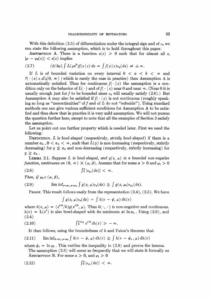
With this definition (2.5) of differentiation under the integral sign and of v, we can state the following assumption, which is to hold throughout this paper.

ASSUMPTION A. There is a function e(z) > 0 such that for almost all z, tso- so(z)I < e(z) implies

(2.7) (a/lap) f L(pss)f(s I z) ds = f(s I z)v(ds) 5 i m.

If L is of bounded variation on every interval 0 < a < b < oo and f( * I z) e oCo(O 0 oo) (which is rarely the case in practice) then Assumption A is automatically satisfied. Thus for continuous f( * I z) the assumption is a con- dition only on the behavior of L( * ) and of f( * I z) near 0 and near oo. (Near 0 it is usually enough just for f to be bounded since i', will usually satisfy (2.8).) But Assumption A may also be satisfied if f( * I z) is not continuous (roughly speak- ing so long as "uncontinuities" of f and of L do not "coincide"). Using standard methods one can give various sufficient conditions for Assumption A to be satis- fied and thus show that in practice it is very mild assumption. We will not pursue the question further here, except to note that all the examples of Section 3 satisfy the assumption.

Let us point out one further property which is needed later. First we need the following:

DEFINITION. L is bowl-shaped (respectively, strictly bowl-shaped) if there is a number aL , 0 < aL < oo, such that L(y) is non-increasing (respectively, strictly decreasing) for y < aL and non-decreasing (respectively, strictly increasing) for y ? aL.

LEMMA 2.1. Suppose L is bowl-shaped, and g(s, A) is a bounded non-negative function, continuous on (0, oo ) X (a, ,B). Assume that for some a > 0 and sp1 > 0

(2.8) fOf IvKo(ds)I < oo.

Then, if ,-o e (a, 3),

(2.9) lim infp,,p1,1,,;0 f g(s, y)g (ds) _ f g(s, 1Ao)zf1(ds).

PROOF. This result follows easily from the representation (2.4), (2.5). We have

f g(s, p_)zi,(ds) = f h(v- , ,u) dX(v)

where h(v, ,0) = (evIk/k)g(evIk, ,;). Thus h(*, *) is non-negative and continuous. X(v) = L(e') is also bowl-shaped with its minimum at ln aL. Using (2.8), and (2.4)

(2.10) fnaL evk dX(v) > -oo.

It then follows, using the boundedness of h and Fatou's theorem that

(2.11) liminfp4^4,,X0 f h(v - /, /t) dX(v) > f h(v -1, g) dX(v)

where l= In (,i . This verifies the inequality in (2.9) and proves the lemma. The assumption (2.8) will occur so frequently that we will state it formally as ASSUMPTION B. For some a > 0, and (pi > 0

34 L. BROWN

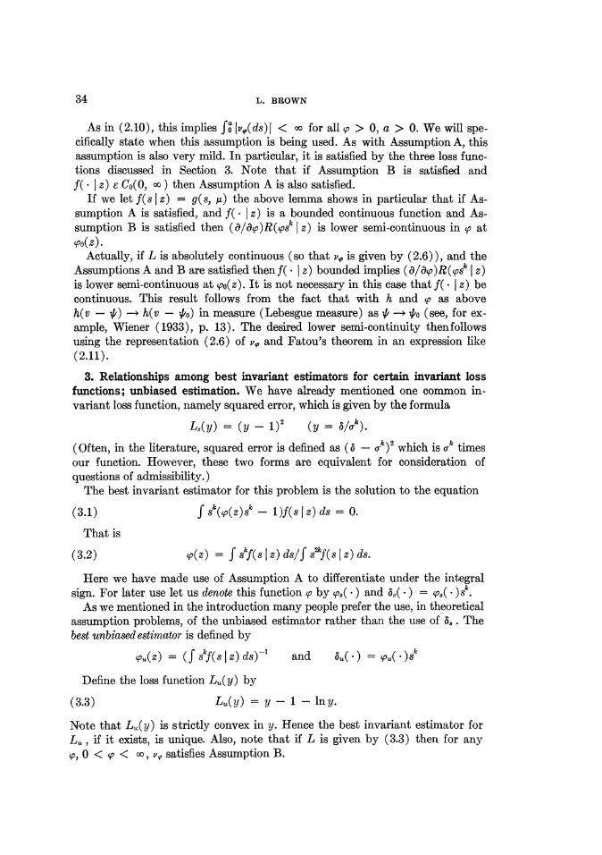
As in (2.10), this implies fo v,(ds)I < oo for all s9 > 0, a > 0. We will spe- cifically state when this assumption is being used. As with Assumption A, this assumption is also very mild. In particular, it is satisfied by the three loss func- tions discussed in Section 3. Note that if Assumption B is satisfied and f( * I z) E C0(O, o ) then Assumption A is also satisfied.

If we let f(s j z) - g(s, A) the above lemma shows in particular that if As- sumption A is satisfied, and f( * I z) is a bounded continuous function and As- sumption B is satisfied then (a/aq9)R(q9sk I z) is lower semi-continuous in p at sPo(z).

Actually, if L is absolutely continuous (so that v, is given by (2.6)), and the Assumptions A and B are satisfied then f( I z) bounded implies (a/a0p)R(psk I z) is lower semi-continuous at (,o(z). It is not necessary in this case that f( * I z) be continuous. This result follows from the fact that with h and (, as above h(v - Vf) -* h(v - ('o) in measure (Lebesgue measure) as (1 --* Vto (see, for ex- ample, Wiener (1933), p. 13). The desired lower semi-continuity thenfollows using the representation (2.6) of v, and Fatou's theorem in an expression like (2.11).

3. Relationships among best invariant estimators for certain invariant loss functions; unbiased estimation. We have already mentioned one common in- variant loss function, namely squared error, which is given by the formula

L,(y) = (y - 1)' (y = 6/ -

(Often, in the literature, squared error is defined as ( - a;k)2 which is ak times our function. However, these two forms are equivalent for consideration of questions of admissibility.)

The best invariant estimator for this problem is the solution to the equation

(3.1) f s(P(z)sk _ 1)f(s z) ds = 0.

That is

(3.2) ep(z) = f skf(s I z) ds/f skf(s I z) ds.

Here we have made use of Assumption A to differentiate under the integral sign. For later use let us denote this function (, by p, ( * ) and 6S( * ) -Ps ( . )sk.

As we mentioned in the introduction many people prefer the use, in theoretical assumption problems, of the unbiased estimator rather than the use of 68. The best unbiased estimator is defined by

(Z) = ( skf(s I z) ds)-1 and Su(*) k

Define the loss function Lu(y) by

(3.3) Lu(y) = y - 1 - Iny.

Note that L.(y) is strictly convex in y. Hence the best invariant estimator for LU, if it exists, is unique. Also, note that if L is given by (3.3) then for any $9, 0 < (o < co, vq, satisfies Assumption B.

INADMISSIBILITY OF ESTIMATORS 35

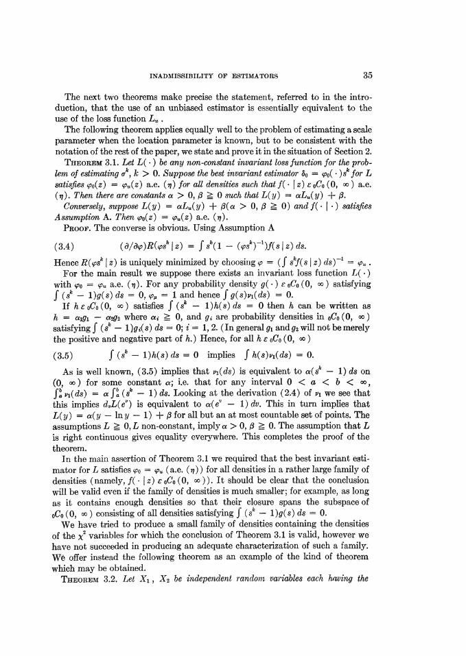
The next two theorems make precise the statement, referred to in the intro- duction, that the use of an unbiased estimator is essentially equivalent to the use of the loss function Lu .

The following theorem applies equally well to the problem of estimating a scale parameter when the location parameter is known, but to be consistent with the notation of the rest of the paper, we state and prove it in the situation of Section 2.

THEOREM 3.1. Let L( . ) be any non-constant invariant loss function for the prob- lem of estimating a k, k > 0. Suppose the best invariant estimator 6o = 'Po( * )sk for L satisfies epo(z) - pu(z) a.e. (X) for all densities such that fQ( I z) E oCo (0, oo ) a.e. (rq). Then there are constants a > 0, ( >_ 0 such that L(y) = aLu(y) + (.

Conversely, suppose L(y) = aLu(y) + (3(a > 0, ( ? 0) and f( *) satisfies Assumption A. Then 'po(z) - pu(z) a.e. (n1).

PROOF. The converse is obvious. Using Assumption A

(3.4) ((/8p)R((Sk I Z) = f Sk( - ((sk)l)f(s I z) ds.

Hence RQ(sk I z) is uniquely minimized by choosing qp = (f skf(s I z) ds)' . For the main result we suppose there exists an invariant loss function L(*)

with soo = 'pu a.e. (,I). For any probability density g( * ) e oCo (0, oo ) satisfying f (sk - 1)g(s) ds = 0, p, = 1 and hence f g(s)vl(ds) = 0.

If h e oCo (0, c ) satisfies f (sk - 1)h(s) ds = 0 then h can be written as h = algi - a2g2 where ai 0, and gi are probability densities in oCo (0, oo ) satisfying f (s8 - 1 )gi( s) ds 0; i = 1, 2. (In general gi and g2 will not be merely the positive and negative part of h.) Hence, for all h e oCo (0, 00 )

(3.5) f (Sk _ 1)h(s) ds = 0 implies f h(s)vl(ds) = 0.

As is well known, (3.5) implies that vi(ds) is equivalent to a(sk - 1) ds on (0, oo) for some constant a; i.e. that for any interval 0 < a < b < oo, fa vi(ds) = a fa (Sk - 1) ds. Looking at the derivation (2.4) of Pi we see that this implies dvL(ev) is equivalent to a(ev - 1) dv. This in turn implies that L(y) = a(y - lny - 1) + , for all but an at most countable set of points. The assumptions L > 0, L non-constant, imply a > 0, A > 0. The assumption that L is right continuous gives equality everywhere. This completes the proof of the theorem.

In the main assertion of Theorem 3.1 we required that the best invariant esti- mator for L satisfies (po = <pu ( a.e. (n) ) for all densities in a rather large family of densities (namely, fA I z) e oCo (0, oo )). It should be clear that the conclusion will be valid even if the family of densities is much smaller; for example, as long as it contains enough densities so that their closure spans the subspace of OCO (0, co ) consisting of all densities satisfying f (k _-1 )g( s) ds = 0.

We have tried to produce a small family of densities containing the densities of the x2 variables for which the conclusion of Theorem 3.1 is valid, however we have not succeeded in producing an adequate characterization of such a family. We offer instead the following theorem as an example of the kind of theorem which may be obtained.

THEOREM 3.2. Let Xi, X2 be independent random variables each having the

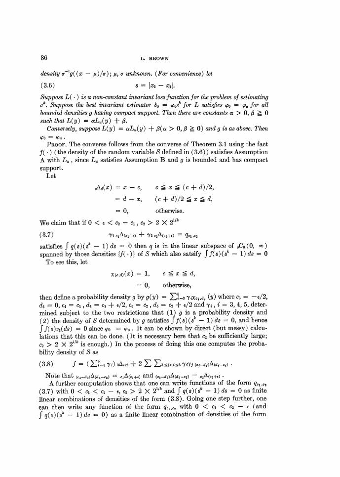
36 L. BROWN

density v-1'g( (x- )/o); ,u, o unknown. (For convenience) let

(3.6) s = X2- xi

Suppose L(*) is a non-constant invariant loss function for the problem of estimating crk. Suppose the best invariant estimator do = 5pok for L satisfies 'po = (p, for all bounded densities g having compact support. Then there are constants a > 0, d > 0 such that L(y)= aLu(y) + i.

Conversely, suppose L(y) = czLu(y) + f3(ac > 0, /3 > 0) and g is as above. Then

(Po Pu.

PROOF. The converse follows from the converse of Theorem 3.1 using the fact f( * ) (the density of the random variable S defined in (3.6)) satisfies Assumption A with Lu, since Lu satisfies Assumption B and g is bounded and has compact support.

Let

cAd(X) = X-C, C c X-< (c + d)/2,

=d-x, (c+d)/2<x<di

= O, otherwise.

We claim that if 0 < E < C2 - C1, C2 > 2 X 211k

(3.7) 'y'C1A(c1+e) + 'Y2C2A(c2+0 = qc,1,C2

satisfies I q(s)(Sk - 1) ds = 0 then q is in the linear subspace of oCo (0, oo)

spanned by those densities {f( * ) of S which also satsify J f(s) (Sk _ 1) ds = 0 To see this, let

X(c,d)(X) =, c < X ? d, = O, otherwise,

then define a probability density g by g(y) = ES= 7Y%Xs,di (y) where C3 = e/2, 03 , C4 c , d4 = cl + E/2, c6 = C2, d5 = c2 + E/2 and ay, i = 3, 4, 5, deter-

mined subject to the two restrictions that (1) g is a probability density and (2) the density of S determined by g satisfies f f(S) (Sk - 1) ds = 0, and hence

f f(s)v'(ds) = 0 since oo = 'P . It can be shown by direct (but messy) calcu- lations that this can be done. (It is necessary here that c2 be sufficiently large; c2 > 2 X 21/k is enough.) In the process of doing this one computes the proba- bility density of S as

(3.8) f = (E !Y3i) OAe/2 + 2 Z Z3?1<?5 YYj (cj-diA(d3-ci)

Note that (C4-d3)A(d4-c3) cL(ci+e and (cd3)A(d5C3) A2+

A further computation shows that one can write functions of the form qcl,c2

(3.7) with 0 < cl < c2 - E, c2 > 2 X 2"lk and f q(s)(sk - 1) ds = 0 as finite linear combinations of densities of the form (3.8). Going one step further, one can then write any function of the form q,1,C2 with 0 < cl < c2 - e (and f q(s) (5k - 1) ds = 0) as a finite linear combination of densities of the form

INADMISSIBILITY OF ESTIMATORS 37

(3.8). These functions, qcl,C2, are clearly dense in the uniform norm in the sub- space of functions in oCo (a, b) satisfying J h(s) (Sk - 1) ds = 0. It follows that vi satisfies the statement (3.5) in the proof of Theorem 3.1.

Thus, just as in Theorem 3.1 it now follows that L(y) = aLu(y) + A, a > 0, a ? 0. This completes the proof of the theorem.

These two theorems should not be interpreted as an argument that L" is in- herently a more reasonable loss function for this problem than squared error (L8). Rather, the loss function to be used in any particular situation should de- pend on as accurate an assessment as possible of the actual losses which will be incurred in that situation. We feel, however, that theorems such as the above may aid in the choice of which loss function to use in some general situations.

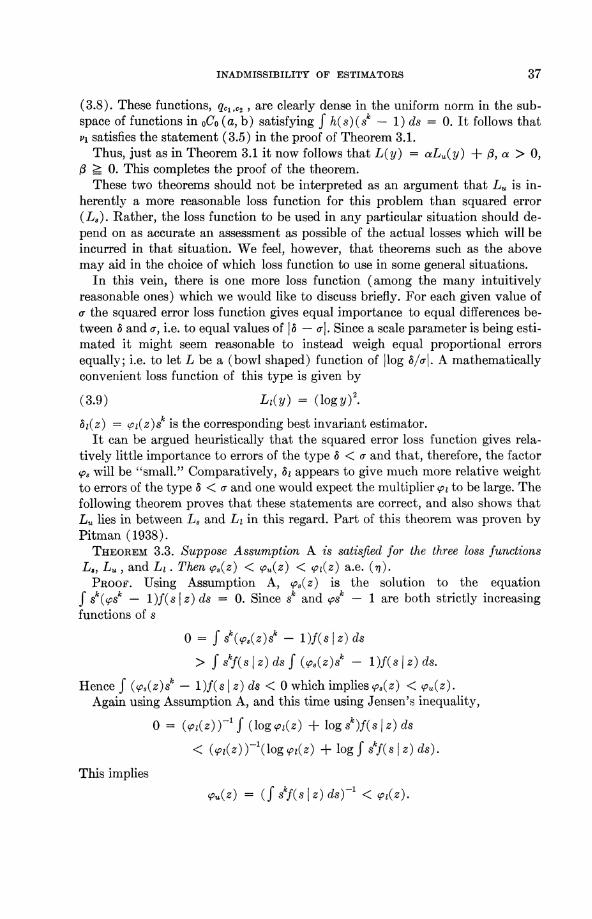
In this vein, there is one more loss function (among the many intuitively reasonable ones) which we would like to discuss briefly. For each given value of a the squared error loss function gives equal importance to equal differences be- tween a and a-, i.e. to equal values of 18 - -1. Since a scale parameter is being esti- mated it might seem reasonable to instead weigh equal proportional errors equally; i.e. to let L be a (bowl shaped) function of Ilog b/lo1. A mathematically convenient loss function of this type is given by

(3.9) Li(y) = (logy)2.

b8(z) = <p1(z)sk is the corresponding best invariant estimator. It can be argued heuristically that the squared error loss function gives rela-

tively little importance to errors of the type 8 < o- and that, therefore, the factor sp, will be "small." Comparatively, 8z appears to give much more relative weight to errors of the type 6 < o- and one would expect the multiplier s0 to be large. The following theorem proves that these statements are correct, and also shows that L. lies in between L8 and L, in this regard. Part of this theorem was proven by Pitman (1938).

THEOREM 3.3. Suppose Assumption A is satisfied for the three loss functions L8, LU, and Li. Then (p8(z) < (pU(z) < (pI(z) a.e. (q).

PROOF. Using Assumption A, sp8(z) is the solution to the equation sk((ps - 1)f(s I z) ds = 0. Since Sk and fk - 1 are both strictly increasing

functions of s

0 = sk(P(z)sk - 1)f(s I z) ds

> f skf(s I z) ds f (c(Z)sk - l)f(s z) ds.

Hence f (<S0(z)sk - 1)f(s I z) ds < 0 which implies cp,(z) < fou(z). Again using Assumption A, and this time using Jensen's inequality,

0 = (fI(z) )-r f (log <P1(Z) + log Sk)f(S I z) ds < (<z(z)'O(log 1(z) + logf skf(s I z) ds).

This implies

cpu(z) = (f skf(sIz)ds)-l < z(z).

38 L. BROWN

This completes the proof of the theorem.

4. Inadmissibility results for normal random variables, and generalizations. If X1, *... X. are independent normal random variables with mean ,u and variance 2 then t = x and s as defined in (2.1) are sufficient statistics. Hence their distribution does not depend on z, and neither does the best invariant esti- mator. However this fact does not play a role in the methods of this section. What is crucial for the results of this section is the fact that T and S are inde- pendent (conditionally on z).

Theorem 4.1 contains the condition that

(4.1) fo,i(s, t z) =f(s i z)h(t I z)

where, of course, both f( * I z) and h( * I z) are probability densities. Therefore this theorem applies to the normal distribution case mentioned above. (The other assumptions of the theorem are easily seen to be also satisfied in the normal distribution case so lonig as L(y) does not tend to infinity extremely fast as y ---0or y --) co.)

As mentioned in the introduction the scale invariant estimators which we will prove to be better than the best invariant estimator are of the form

(4.2) 6,(.) = 0(z)sk if It/sl < K(z)

- Po(z)sk if It/sl > K(z)

where (as always) po(Z) 8k is the best invariant estimator of ak, and @(z) < qo(z). We will have to consider various conditional densities; and so we define (for

example)

(4.3) f( * I it/sI < K, , z)

to be the conditional probability density of S given it/sl < K, and Z = z, for the given value of ,u (and for a = 1). For any scale invariant 6 we also define

(4.4) R(5; A i lt/sl < K, z) = Eu,1(L(S( . )/lak)I It/si < K, Z = z).

It should be clear already that what we will do is to prove that for each given value of Z

(4.5) R( bi , I z)-=R(36;,u I |t/s| < oo, z) <_!! R( So; z)

with strict inequality for an appropriate set of values of Au, which in our case will include a neighborhood of A = 0. (The first equality of (4.5) defines R( 51 ; A I z).) Since we only need to prove (4.5) separately for each given value of Z it will be convenient in the remainder of this section to assume that a value z of Z has been given. We will make this assumptio'n throughout this section except in the statement of Theorem 4.1, and hence we will not write the given value of Z in expressions like (4.1)-(4.5). For example, the expression (4.1) becomes

fo,j(s, t) - f(s)h(t)- The main idea of the proof is, roughly speaking, to show that

f s I It/sl < K, A, z) has a uniform (in ,A) strict monotone likelihood ratio property

INADMISSIBILITY OF ESTIMATORS 39

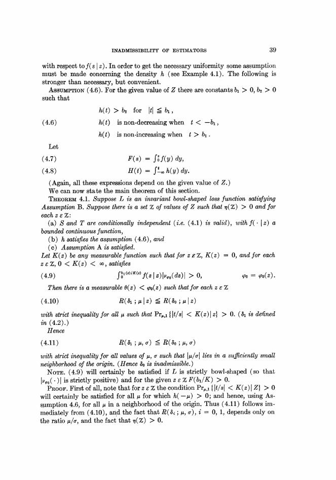
with respect to f( s i z). In order to get the necessary uniformity some assumption must be made concerning the density h (see Example 4.1). The following is stronger than necessary, but convenient.

ASSUMPTION (4.6). For the given value of Z there are constants b1 > 0, b2 > 0

such that

h(t) > b2 for |tl < bi,

(4.6) h(t) is non-decreasing when t < -b1,

h(t) is non-increasing when t > b1 .

Let

(4.7) F(s) = fJf(y) dy,

(4.8) H(t) = f X h(y) dy.

(Again, all these expressions depend on the given value of Z.) We can now state the main theorem of this section. THEOREM 4.1. Suppose L is an invariant bowl-shaped loss function satisfying

Assumption B. Suppose there is a set Z of values of Z such that ?1(Z) > 0 and for each z e Z:

(a) S and T are conditionally independent (i.e. (4.1) is valid), with f(* z) a bounded continuous function,

(b) h satisfies the assumption (4.6), and (c) Assumption A is satisfied.

Let K(z) be any measurable function such that for z r Z, K(z) = 0, and for each z e Z, 0 < K(z) < oo, satisfies

(4.9) rOl(z)K(z) f(s I z) IvSO.(ds)I > 0, o = p(z)O

Then there is a measurable @(z) < 0po(z) such that for each z e Z

(4.10) R(6i;jIz) < R(Oo; tIz)

with strict inequality for all .t such that Pr,,, { It/sI < K(z) I z} > 0. ( 61 is defined in (4.2).)

Hence

(4.11) R(61; t, o) < R(6o; t, a-)

with strict inequality for all values of j.t, o- such that I,tl/oI lies in a sufficiently small neighborhood of the origin. (Hence Oo is inadmissible.)

NOTE. (4.9) will certainly be satisfied if L is strictly bowl-shaped (so that vs,o( * )I is strictly positive) and for the given z c Z F(b1/K) > 0.

PROOF. First of all, note that for z e Z the condition Pr,,1l { It/sl < K(z) I Z} > 0 will certainly be satisfied for all 4 for which h( - i) > 0; and hence, using As-

s,umption 4.6, for all ,u in a neighborhood of the origin. Thus (4.11) follows im- mediately from (4.10), and the fact that R(6Si; Ilu, o), i = 0, 1, depends only on the ratio ,u/o-, and the fact that 71(Z) > 0.

40 L. BROWN

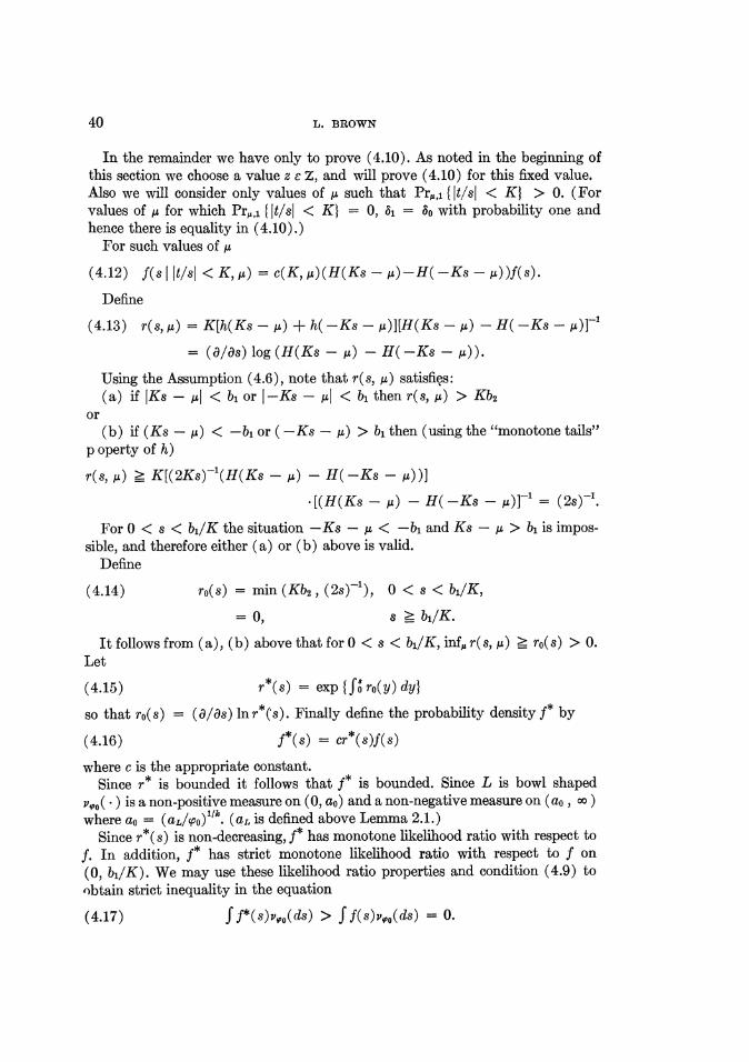
In the remainder we have only to prove (4.10). As noted in the beginning of this section we choose a value z E Z, and will prove (4.10) for this fixed value. Also we will consider only values of ,u such that Pr,,1,{ lt/sl < K} > 0. (For values of ,t for which Pr,,, { lt/sl < K} = 0, &1 = Oo with probability one and hence there is equality in (4.10).)

For such values of ,u

(4.12) f(sj It/sl < K,,i) = c(K,M)(H(Ks - 1.t)-H(-Ks - i))f(s).

Define

(4.13) r(s,) = K[h(Ks - ,.) + h(- Ks - t)][H(Ks - z) - H(- Ks -

= (a/as) log (H(Ks - t) - H(-Ks - 1)).

Using the Assumption (4.6), note that r(s, ,u) satisfies: (a) if IKs - .j < b1 or |-Ks - pI < bi then r(s,) > Kb2

or (b) if (Ks - ,.) < -bi or ( -Ks - A) > bi then (using the "monotone tails"

p operty of h)

r(s, /.) > K[(2Ks)-1(H(Ks - y) - H(-Ks - t))]

.[(H(Ks - y) - H(-Ks - tz)]-1 = (2s)-'.

For 0 < s < b1/K the situation -Ks - y < -bi and Ks - / > bi is impos- sible, and therefore either (a) or (b) above is valid.

Define

(4.14) ro(s) = mnu (Kb2, (2s)-1), 0 < s < b1/K,

= O, s > b/K.

It follows from (a), (b) above that for 0 < s < b1/K, inf, r(s,,u) > ro(s) > 0. Let

(4.15) r*(s) = exp{J'oro(y)dy}

so that ro(s) = (a/as) ln r*(s). Finally define the probability density f* by

(4.16) f*(s) = cr*(s)f(s)

where c is the appropriate constant. Since r* is bounded it follows that f* is bounded. Since L is bowl shaped

vIO ( * ) is a non-positive measure on (0, ao) and a non-negative measure on (ao, oo) where ao = (aL/po0)l/k. (aL is defined above Lemma 2.1.)

Since r*(s) is non-decreasing, f* has monotone likelihood ratio with respect to f. In addition, f* has strict monotone likelihood ratio with respect to f on (0, b1/K). We may use these likelihood ratio properties and condition (4.9) to obtain strict inequality in the equation

(4.17) ff*(s)vvo(ds) > ff(s)vp0(ds) = 0.

INADMISSIBILITY OF ESTIMATORS 41

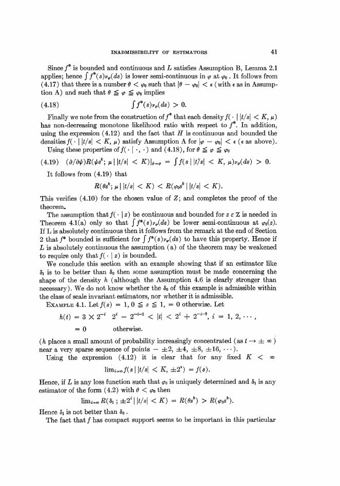
Since f* is bounded and continuous and L satisfies Assumption B, Lemma 2.1 applies; hence f f*(s)v,(ds) is lower semi-continuous in so at soo . It follows from (4.17) that there is a number 0 < spo such that 1 - sool < e (with e as in Assump- tion A) and such that a < so po implies

(4.18) f f*(s)v(ds) > 0.

Finally we note from the construction of f* that each density f( - I tl/sI < K, A) has non-decreasing monotone likelihood ratio with respect to f*. In addition, using the expression (4.12) and the fact that H is continuous and bounded the densities f( * I lt/sl < K, A) satisfy Assumption A for iso - sool < E (E as above).

Using these properties of f(* I *, - ) and (4.18), for 6 <? s <_ _o

(4.19) (a/AaI)RG lsk;,ulit/sl < K)i=,, = ff(s I it%si < K, ,)vp(ds) > 0.

It follows from (4.19) that

R(s; ,ua I It/sf < K) < R(posk I it/sl < K).

This verifies (4.10) for the chosen value of Z; and completes the proof of the theorem.

The assumption that f( * z) be continuous and bounded for z E Z is needed in Theorem 4.1(a) only so that f f*(s)v,(ds) be lower semi-continuous at soo(z). If L is absolutely continuous then it follows from the remark at the end of Section 2 that f* bounded is sufficient for f f*(s)v,(ds) to have this property. Hence if L is absolutely continuous the assumption (a) of the theorem may be weakened to require only that f( - i z) is bounded.

We conclude this section with an example showing that if an estimator like 61 is to be better than So then some assumption must be made concerning the shape of the density h (although the Assumption 4.6 is clearly stronger than necessary). We do not know whether the So of this example is admissible within the class of scale invariant estimators, nor whether it is admissible.

ExAMPLE 4.1. Let f(s) = 1, 0 < s < 1, = 0 otherwise. Let

h(t) = 3 X 2-' 2i - 27$-2 < itl < 2' + 2-i-2 i =1, 2,...

= 0 otherwise.

(h places a small amount of probability increasingly concentrated (as t -* ? ) near a very sparse sequence of points -2, +4, +8, +16, ***).

Using the expression (4.12) it is clear that for any fixed K < oo

limo,wf(s I lt/sl < K, +2t) = f(s).

Hence, if L is any loss function such that soo is uniquely determined and &1 is any estimator of the form (4.2) with 0 < soo then

limi, R(31 ; 42' I ft/sl < K) = R(Osk) > R(ooSk).

Hence 8, is not better than 6o. The fact that f has compact support seems to be important in this particular

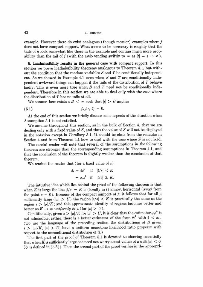
42 L. BROWN

example. However there do exist analagous (though messier) examples where f does not have compact support. What seems to be necessary is roughly that the tails of h look somewhat like those in the example and contain much more prob-

ability than the tail of f (with the ratio tending swiftly to oo as ftl = s -oo ).

5. Inadmissibility results in the general case with compact support. In this section we prove inadmissibility theorems analogous to Theorem 4.1, but with- out the condition that the random variables S and T be conditionally independ- ent. As we showed in Example 4.1 even when S and T are conditionally inde- pendent awkward things can happen if the tails of the distribution of T behave badly. This is even more true when S and T need not be conditionally inde- pendent. Therefore in this section we are able to deal only with the case where the distribution of T has no tails at all.

We assume here exists a B < oo such that Itf > B implies

(5.1) fo, (s, t) 0.

At the end of this section we briefly discuss some aspects of the situation when Assumption 5.1 is not satisfied.

We assume throughout this section, as in the bulk of Section 4, that we are dealing only with a fixed value of Z, and thus the value of Z will not be displayed in the notation except in Corollary 5.1. It should be clear from the remarks in Section 4 and from Theorem 4.1 how to deal with the case where Z is not fixed.

The careful reader will note that several of the assumptions in the following theorem are stronger than the corresponding assumptions in Theorem 4.1, and that the conclusion of the theorem is slightly weaker than the conclusion of that theorem.

We remind the reader that (for a fixed value of z)

- Osk if t/sl < K

0os k if ft/sf > K.

The intuitive idea which lies behind the proof of the following theorem is that when K is large the line |t/s| = K is (locally in t) almost horizontal (away from the point s 0). Because of the compact support of f; it follows that for all A sufficiently large (J AI > U) the region ft/sl < K is practically the same as the region s > 1,MI/K; and this approximate identity of regions becomes better and better as K -* oo uniformly in ,u (for M I > U) .

Conditionally, given s > Mu/K for MII, > U, it is clear that the estimator Os is not admissible; rather, there is a better estimator of the form Os' with 0 < oo. (To use the language of the preceding section the distributions of S given s > MI4/K, I ul > U, have a uniform monotone likelihood ratio property with respect to the unconditional distribution of S.)

The first part of the proof of Theorem 5.1 is devoted to showing essentially that when K is sufficiently large one need not worry about values of M with MIAI < U

(U is defined in (5.8)). Then the second part of the proof verifies in the appropri-

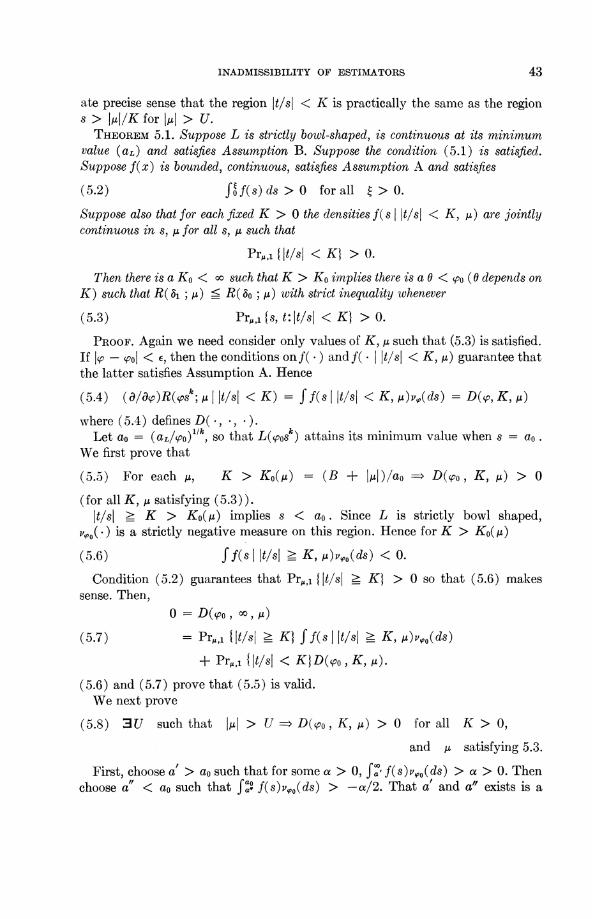
INADMISSIBILITY OF ESTIMATORS 43

ate precise sense that the region ft/sl < K is practically the same as the region s > 11t1/K for 1f1 > U.

THEOREM 5.1. Suppose L is strictly bowl-shaped, is continuous at its minimum value (aL) and satisfies Assumption B. Suppose the condition (5.1) is satisfied. Suppose f(x) is bounded, continuous, satisfies Assumption A and satisfies

(5.2) ff(s) ds > 0 for all > O.

Suppose also that for each fixed K > 0 the densities f(s f lt/sl < K, ,u) are jointly continuous in s, ,u for all s, ,u such that

Pr,,, Iltlsl <X}I >O0.

Then there is a Ko < oo such that K > Ko implies there is a 0 < ypo (0 depends on K) such that R( ; ,u) < R( o; a,) with strict inequality whenever

(5.3) Pr,,,, s, t: I ts I < K}I > O.

PROOF. Again we need consider only values of K, 1i such that (5.3) is satisfied. If ko - sof < e, then the conditions onf(.) andf( f I lt/sf < K, Pt) guarantee that the latter satisfies Assumption A. Hence

(5.4) (a/O<)R(psk;,41 ft/sl < K) = ff(s I ft/sl < K, P)v,(ds) = D(p, K, P)

where (5.4) defines D( , , ). Let ao = (aL/oo)llk, so that L(svosk) attains its minimum value when s = ao .

We first prove that

(5.5) For each Pt, K > Ko(,u) = (B + fPtf)/ao > D(0po, K, Pt) > 0

(for all K, Pt satisfying (5.3)). ft/sl ? K > Ko(Pt) implies s < ao. Since L is strictly bowl shaped,

v,po(.) is a strictly negative measure on this region. Hence for K > Ko(P)

(5.6) ff(s Ift/sl > K, P)v,o(ds) < 0.

Condition (5.2) guarantees that PrM,l {ft/sf > K} > 0 so that (5.6) makes sense. Then,

0 = D(0po *, Pt)

(5.7) = PrM,l {ft/sl > K} rff(s ft/s| > K, P)vo(ds)

+ Pr,, {f t/sl < K} D(po , K, Pt).

(5.6) and (5.7) prove that (5.5) is valid. We next prove

(5.8) 3U such that fPtf > U > D(po, K, Pt) > 0 for all K > 0,

and Pt satisfying 5.3.

First, choose a' > ao such that for some a > 0, f{' f(s)v<,o(ds) > ax > 0. Then choose a' < aO such that Jfa f(s)vvO(ds) > -ca/2. That a' and a" exists is a

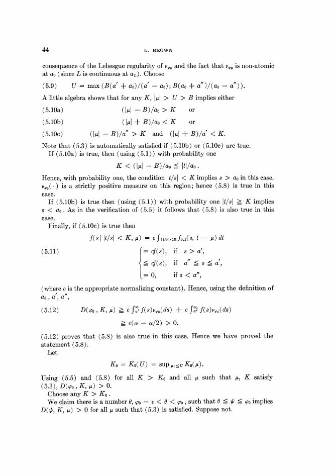
44 L. BROWN

consequence of the Lebesgue regularity of vP00 and the fact that v,, is non-atomic at ao (since L is continuous at aL). Choose

(5.9) U = max (B(a' + ao)/(a' - ao); B(ao + a")/(ao - a")).

A little algebra shows that for any K, 1,u1 > U > B implies either

(5.10a) (I1/l - B)/ao > K or

(5.10b) (JAI + B)/ao < K or

(5.10c) (JAI - B)/a" > K and (1,u1 + B)/a' < K.

Note that (5.3) is automatically satisfied if (5.10b) or (5.10c) are true. If (5.10a) is true, then (using (5.1)) with probability one

K < (1 ul- B)/ao ?< tl/ao.

Hence, with probability one, the condition It/sl < K implies s > ao in this case.

v,0( () is a strictly positive measure on this region; hence (5.8) is true in this case.

If (5.10b) is true then (using (5.1)) with probability one Jt/sl > K implies s < ao. As in the verification of (5.5) it follows that (5.8) is also true in this case.

Finally, if (5.lOc) is true then

f(s I |t/s| < K, ,u) = C fIt/sI<Kf0,1(S t - dt

(5.11) = cf(s), if s > a',

< cf (s), if a"

< s <

a'

t= 0, if s < a",

(where c is the appropriate normalizing constant). Hence, using the definition of aO, a, a",

(5.12) D((po, K, A) _ c f?' f(s)v,0(ds) ? c Ja f(s)v,0(ds)

> c(Ca - oa/2) > 0.

(5.12) proves that (5.8) is also true in this case. Hence we have proved the statement (5.8).

Let

Ko = Ko( U) = sup1j,? u Ko((A).

Using (5.5) and (5.8) for all K > Ko and all ,u such that ,u, K satisfy (5.3), D(Spo, K, ,) > 0.

Choose any K > Ko. We claim there is a number 0, o - E < a < spo, such that 0 < i1 ? spo implies

D(AV, K, ,u) > 0 for all , such that (5.3) is satisfied. Suppose not.

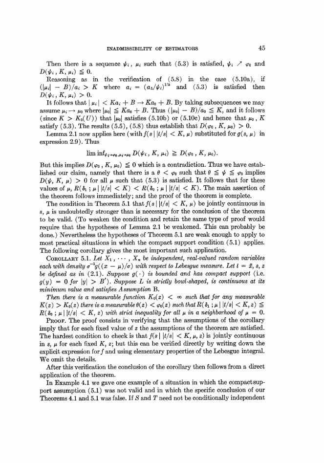
INADMISSIBILITY OF ESTIMATORS 45

Then there is a sequence /i, 4ii such that (5.3) is satisfied, 41i A 'po and

D(41i IK, Ai) _O< . Reasoning as in the verification of (5.8) in the case (5.10a), if

(1,2l - B)/ai > K where ai = (aL/1i)lIk and (5.3) is satisfied then D)(4i IK, ju) > 0.

It follows that I Ai I < Kai + B - Kao + B. By taking subsequences we may assume i -* /2o where lIol ? Kao + B. Thus (1IMuol - B)/ao ? K, and it follows (since K > Ko(U)) that l10ol satisfies (5.10b) or (5.10c) and hence that Muo, K satisfy (5.3). The results (5.5), (5.8) thus establish that D(qpo, K, ,o) > 0.

Lemma 2.1 now applies here (with f(s j It/sI < K, p) substituted for g(s, ,) in expression 2.9). Thus

lim infpi_,p0,i_ D(4/', K, Ai) > D(Qpo, K, Mo).

But this implies D(po, K, ,uo) < 0 which is a contradiction. Thus we have estab- lished our claim, namely that there is a 0 < spo such that 0 ?< i1 ?< 'o implies D(4t, K, M) > 0 for all A such that (5.3) is satisfied. It follows that for these values of A, R(61 ; , II t/sI < K) < R(6o; , I I t/sI < K). The main assertion of the theorem follows immediately; and the proof of the theorem is complete.

The condition in Theorem 5.1 that f(s I It/sl < K, A) be jointly continuous in s, M is undoubtedly stronger than is necessary for the conclusion of the theorem to be valid. (To weaken the condition and retain the same type of proof would require that the hypotheses of Lemma 2.1 be weakened. This can probably be done.) Nevertheless the hypotheses of Theorem 5.1 are weak enough to apply to most practical situations in which the compact support condition (5.1) applies. The following corollary gives the most important such application.

COROLLARY 5.1. Let X1, ***, X. be independent, real-valued random variables each with density -lg( (x - M)/l) with respect to Lebesgue measure. Let t = x, s, z be defined as in (2.1). Suppose g(.) is bounded and has compact support (i.e. g(y) = 0 for JyI > B'). Suppose L is strictly bowl-shaped, is continuous at its minimum value and satisfies Assumption B.

Then there is a measurable function Ko(z) < oo such that for any measurable K(z) > Ko(z) there is a measurable 0(z) < 'po(z) such that R(fi1; ,M I lt/sl < K, z) <

R( 6o ; , I It/sI < K, z) with strict inequality for all M in a neighborhood of M = 0. PROOF. The proof consists in verifying that the assumptions of the corollary

imply that for each fixed value of z the assumptions of the theorem are satisfied. The hardest condition to check is that f(s I It/sI < K, u, z) is jointly continuous in s, M for each fixed K, z; but this can be verified directly by writing down the explicit expression for f and using elementary properties of the Lebesgue integral. We omit the details.

After this verification the conclusion of the corollary then follows from a direct application of the theorem.

In Example 4.1 we gave one example of a situation in which the compact sup- port assumption (5.1) was not valid and in which the specific conclusion of our Theorems 4.1 and 5.1 was false. If S and T need not be conditionally independent

46 L. BROWN

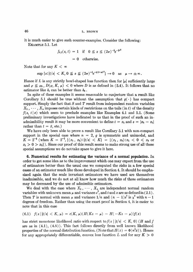
it is much easier to give such counter-examples. Consider the following: EXAMPLE 5.1. Let

fo,(s, t) = 1 if 0 < s ?

= 0 otherwise.

Note that for any K < oo

sup {s: It/sI < K, 0 < s < (27r) e-(ty)2} -O0 as ,u i oo .

Hence if L is any strictly bowl-shaped loss function then for Jlpl sufficiently large and so < soo, D(p, K, A) < 0 where D is as defined in (5.4). It follows that no estimator like &, can be better than 6S.

In spite of these examples it seems reasonable to cQnjecture that a result like Corollary 5.1 should be true without the assumption that g( * ) has compact support. Simply the fact that S and T result from independent random variables Xi, * * *, X,, imposes certain kinds of restrictions on the tails (in t) of the density f(s, t I z) which seem to preclude examples like Examples 4.1 and 5.1. (Some preliminary investigations have indicated to us that in the proof of such an in- admissibility result it may be more convenient to define t- x and s = x2- xil rather than t = x, etc.)

We have only been able to prove a result like Corollary 5.1 with non-compact support in the special case where n = 2, g is symmetric and unimodal, and K = 2- (when K = 2-, {(xi, x2):It/sI < K} = {(xl, x2):xl < 0 < x2 or xl > 0 > x2} ) . Since our proof of this result seems to make strong use of all these special assumptions we do not take space to give it here.

6. Numerical results for estimating the variance of a normal population. In order to get some idea as to the improvement which one may expect from the use of estimators better than the usual one we computed the risks in a few special cases of an estimator much like those developed in Section 4. It should be empha- sized again that the scale invariant estimators we have used are themselves inadmissible, and we do not at all know how much the risks of these estimators may be decreased by the use of admissible estimators.

We deal with the case where X1, ***, X. are independent normal random variables with unknown mean j, and variance 2, and t and s are as defined in (2.1). Then T is normal with mean A and variance 1/n and (n - 1)82 is X2 with n - 1 degrees of freedom. Rather than using the exact proof in Section 4, it is easier to note that in this case

(6.1) f(s I It/sl < K, ,A) = c(K, A)(H(Ks- -H(-Ks - , ))f(s)

has strict monotone likelihood ratio with respect to f( s I It/sl < K, 0) (H and f are as in (4.1), (4.8)). This fact follows directly from well known likelihood properties of the normal distribution function. (Note that H( x) = (D(n x)). Hence for any appropriately differentiable, convex loss function L and for any K > 0

INADMISSIBILITY OF ESTIMATORS 47

the 0 in the definition of 61 (4.2) may be chosen as the unique solution of

(6.2) f S W'(0sk)(H(Ks) - H(-Ks))f(s) ds = 0.

Formula (6.1) can then be used to compute the risk of &1 and this risk can be compared with the risk of 6o.

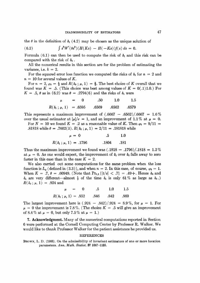
All the numerical results in this section are for the problem of estimating the variance, i.e. k = 2.

For the squared error loss function we computed the risks of 61 for n = 2 and n = 10 for several values of K.

For n = 2, (Po = 1 and R(60 ; ,u, 1) = . The best choice of K overall that we found was K = .5. (This choice was best among values of K = 0(.1)1.0.) For K = .5, 0 as in (6.2) was C = .2794(6) and the risks of &1 were

,u - 0 .50 1.0 1.5

R(S1; Ay 1) -.6595 .6569 .6562 .6579

This represents a maximum improvement of (.6667 - .6562)/.6667 = 1.6% over the usual estimator at jIj/I = 1, and an improvement of 1.1 % at , = 0.

For N = 10 we found K = .2 as a reasonable value of K. Then soo = 9/11 .81818 while 0 = .7602(3). R(6o; , 1) = 2/11 = .181818 while

Au= O .5 1.0

R(61 ;,u 1) = .1796 .1804 .181

Thus the maximum improvement we found was (.1818 - .1796)/.1818 = 1.2 % at ,u = 0. As one would expect, the improvement of 81 over So falls away to zero faster in this case than in the case K = 2.

We also carried out some computations for the same problem when the loss function is L, (defined in (3.3)), and when n = 2. In this case, of course, soo = 1. When K = .7, 0 = .60949. (Note that Prol {I t/sl < .7} = .49+. Hence 8o and &1 are very different-almost 2 of the time 31 is only 61 % as large as 30.) R(So; u, 1) = .924 and

,u = 0 .5 1.0 1.5

R(i; ji, 1) .852 .846 .842 .860

The largest improvement here is (.924 - .842)/.924 = 8.9 %, for , - 1. For u= 0 the improvement is 7.8%. (The choice K = .5 will give an improvement

of 8.4 % at A = 0, but ony 7.5 % at A = 1.)

7. Acknowledgment. Many of the numerical computations reported in Section 6 were performed at the Cornell Computing Center by Professor R. Walker. We would like to thank Professor Walker for the patient assistance he provided us.

REFERENCES

BROWN, L. D. (1966). On the admissibility of invariant estimators of one or more location parameters. Ann. Math. Statist. 37 1087-1135.

48 L. BROWN

BROWN, L. D. (1967). The conditional level of Student's t-test. Ann. Math. Statist. 38 1068- 1071.

FARRELL, R. (1964). Estimators of a location parameter in the absolutely continuous case. Ann. Math. Statist. 35 949-999.

STEIN, C. (1964). Inadmissibility of the usual estimator for the variance of a normal dis- tribution with unknown mean. Ann. Inst. Statist. Math. 16 155-160.

PITMAN, E. J. G. (1938). The estimation of location and scale parameters of a continuous population of any given form. Biometrika 30 391-421.

WIENER, N. (1933). The Fourier Integral and Certain of Its Applications. Cambridge Press, London.