In the Shadows of Great Men: Leadership Turnovers and ...

In the Shadows of Great Men:Leadership Turnovers and Power Dynamics

in Autocracies

Junyan Jiang∗ Tianyang Xi† Haojun Xie‡

Abstract

Political leaders differ considerably in the degree to which they consolidate power, but whatgives rise to these variations still remains under-theorized. This article studies how informalpolitical constraints associated with leadership turnovers shape intra-elite power dynamics.We argue that aging leaders’ efforts to manage the succession problem create an important, yetimpermanent check on the power of subsequent leaders. To test this argument, we use the mas-sive text corpus of Google Ngram to develop a new quantitative measure of power for a globalsample of autocratic regime leaders and elites between 1950 and 2019, and employ a researchdesign that leverages within-leader variations in predecessors’ influence for identification. Weshow that incumbent leaders’ ability to consolidate power becomes more limited when oper-ating in an environment where influential former leaders are present. Further analyses suggestthat the presence of former leaders is most effective in reducing incumbents’ ability to uni-laterally appoint or remove high-level military and civilian personnel. These findings haveimplications for our understanding of the dynamics of power-sharing and institutional changein autocracies.

∗Assistant Professor, Department of Political Science, Columbia University. Email: [email protected].†Assistant Professor, National School of Development, Peking University. Email: [email protected]‡PhD Student, Department of Finance, Chinese University of Hong Kong. Email: [email protected].

hk

1

Electronic copy available at: https://ssrn.com/abstract=3586255

[email protected]

[email protected]

[email protected]

[email protected]

“Even from my sickbed, even if you are going to lower me into the grave and I feel

that something is going wrong, I will get up. Those who believe that after I have left

the government as prime minister, I will go into a permanent retirement really should

have their heads examined.”

— Lee Kuan Yew, on National Day Rally of 1988, two years before he stepped down

as the Prime Minister of Singapore.

1 Introduction

Contrary to the popular perception that they are all almighty despots with unchallenged authority,

political leaders in authoritarian regimes exhibit wide variations in personal power (Baturo 2014;

Geddes 2003; Svolik 2012). While some leaders manage to achieve an unparalleled level of dom-

inance and rule for decades, others have to regularly share power with other elites and step down

“on time” after a few years in office. The varying configurations of power balance within author-

itarian regimes can have profound consequences for domestic governance (Bueno de Mesquita et

al. 2003; Frantz et al. 2020; Wright and Escriba-Folch 2012), as well as for international relations

(Colgan and Weeks 2014; Weeks 2012).

A rapidly expanding body of scholarship has ventured to explain what gives rise to the different

levels of power among autocratic leaders (Boix and Svolik 2013; Brownlee 2007a; Gandhi 2008;

Geddes 2003; Gehlbach and Keefer 2011, 2012; Frantz and Stein 2017; Magaloni 2008; Meng

2020; Reuter 2017). Most of the existing studies take a regime’s formal institutions as the starting

point. The prevailing view in this literature is that authoritarian regimes with strong organizations

and institutional procedures tend to be more successful at curbing incumbent leaders’ despotic

tendencies and sustaining power-sharing arrangements among ruling elites. However, other stud-

ies have noted that, to the extent that institutions are ultimately human creations, their emergence

(or the lack thereof) may be endogenous to deeper, less observable political and coalitional dy-

namics (Pepinsky 2014) and their effectiveness as constraints cannot always be taken for granted

1


(Levitsky and Murillo 2009; Meng 2019). Empirically, we also observe considerable variations in

personal power among leaders from the same regime or even over the tenure of the same leader:

Both Mahathir Mohamad and Xi Jinping, for example, took office under highly institutionalized

party regimes, but managed to build up their personal authority in a way that their immediate

predecessors never could (Li 2016; Slater 2003). Other leaders, like Jiang Zemin in China and

Islam Karimov in Uzbekistan, were initially seen as only weak, transitional figures, but later went

on to rule their respective countries for many years (Ilkhamov 2007; Kuhn 2004). How do we

make sense of these ebbs and flows of power in individual leaders when the broader institutional

variables were largely held constant?

In this article, we provide a new perspective on authoritarian power dynamics by shifting the

focus from the formal institutions to the informal constraints in high-level elite politics. We con-

ceptualize informal constraints as the deeper, and sometimes covert, configurations of actors, net-

works, and coalitions among the ruling elites that exist and operate relatively independent of the

incumbent ruler’s control. We argue that such constraints define important parameters of elite

politics, such as the amount of discretion the incumbent enjoys in making key political decisions,

the size and the kind of patronage resources s/he can control, and the potential consequences for

breaking power-sharing pacts with other elites. Unlike institutions, which are relatively stable over

time, these informal constraints are often dynamic and can constantly evolve in response to many

internal and external factors. The nature and strength of the constraints that incumbent autocrats

face at a given moment set the scope for feasible political strategies, and in turn their ability to

successfully consolidate power.

To demonstrate the utility of this perspective, we study how a particular set of informal con-

straints common in many durable autocracies—the presence of influential senior political figures

from earlier generations—shape incumbent rulers’ power in those regimes. Leadership turnover is

a profoundly important yet highly sensitive issue in authoritarian politics (Burling 1974; Hunting-

ton and Moore 1970; Treisman 2015; Tullock 1987). In regimes that have survived one or more

rounds of successions, new top leaders often enter office with one or several of their predecessors

2


still alive and active. Despite having relinquished much of their formal power, those retired lead-

ers often retain substantial informal influence over politics and policies through the contacts and

networks they cultivated during their time in office. We argue that they can place an informal, yet

important check on the incumbent ruler by serving as the potential key focal points for other elites

to coordinate counter-balancing actions.

We construct a global sample of autocracies between 1950 and 2019 to examine whether the

presence or absence of influential retired leaders affects the personal power of incumbent ruler vis-

a-vis other elites. Empirically, studying intra-regime power dynamics faces two main challenges.

The first one is measurement: It is usually difficult to measure a political leader’s power precisely

and objectively, let alone to compare it across time and different country settings. To overcome this

challenge, we develop a novel measure of personal power for top national leaders by making use

of two massive online databases: Google Books Ngram (Google Ngram hereafter) and Wikidata.

Our approach builds on a burgeoning body of recent literature that uses printed publications to

make inferences about political actors’ power (e.g., Ban et al. 2018; Jaros and Pan 2017). We first

compile a comprehensive list of prominent living politicians for each country–year spell covered

in our sample based on biographical information from Wikidata, and then use Google Ngram to

compute a power index based on the ratio between the number of publications that mention a top

political leader’s name and the number of publications that mention other influential (living) polit-

ical figures from the same country and same year. Through a number of case-by-case comparisons

and systematic validation tests, we show that our measure not only exhibits strong consistency with

the existing measures of regime types, institutional constraints, and personalism, but also does a

better job than the existing measures at capturing the subtle yet important variations in personal

power over a leader’s tenure. We also show that our measure correlates well with various other

outcomes and metrics that are often used as proxies of power, such as tenure length, vote share in

elections, centrality in elite networks, the size of a leader’s personal coalition/faction, and experts’

assessments of leaders’ political influence.

In addition to measurement, the second empirical challenge is causal identification. The pres-

3


ence or absence of retired leaders may be correlated with various other regime characteristics that

can affect an incumbent’s personal power. To overcome this problem, our main empirical design

exploits within-incumbent variations in retired leaders’ strength that come exclusively from the

deaths (mostly natural) of retired leaders. This design essentially removes all the unobserved het-

erogeneity across incumbent leaders, and enables us to focus solely on the change in power within

the same leader before and after the passing of his/her most influential predecessor.

Our empirical results provide strong evidence that retired leaders play a significant role in limit-

ing the personal power of the incumbents. According to our preferred within-person specification,

the presence of a former leader from the same political regime on average reduces the incumbent

autocrat’s power by about 19% of a standard deviation in the short run, and by about 29% of a

standard deviation in the long run. Through a series of additional tests, we show that our findings

are robust to various modifications to the sample coverage, model specifications, and coding of the

dependent and independent variables. We also demonstrate that the estimated effects are not driven

by unobserved shocks common to all leadership turnovers, but are only present for within-regime

transitions wherein predecessors exit power in a relatively consensual fashion.

Finally, we provide some suggestive evidence on how predecessors retain and exercise their

influence in retirement. Our analysis draws on not only the existing measures for regimes’ lead-

ership and institutions but also several new measures of power distribution within regimes’ ruling

cabinets, built by applying our Ngram-based method to a newly available global dataset on cabinet

members (Nyrup and Bramwell 2020). We find that instead of affecting the features of general for-

mal institutions, such as elections, legislatures, or parties, the constraining effect of former leaders

is often exerted in a highly specific and informal way—through limiting the successor’s personal

discretion over the appointment and removal of key supporting elites that are essential to his/her

consolidation of power.

This study advances our understanding of power dynamics in authoritarian regimes in two

important ways. First, we offer a new way to think about how power is shared in authoritarian

regimes. Existing literature typically conceptualizes authoritarian power-sharing in a context-free

4


way as the interaction between a dictator and a group of lesser elites who want to protect their

power from the encroachment of the dictator (Magaloni 2008; Meng 2020; Myerson 2008; Svolik

2009). By contrast, we show that there is a different mode of power-sharing wherein the central

cleavage is organized between current and former autocrats. We provide evidence that the inter-

generational model may be more effective in constraining the behaviors of incumbents than an

intra-generational one because of the involvement of more senior political actors. However, these

inter-generational constraints are also inherently uncertain and impermanent because they depend

heavily on the personal conditions of former leaders.

Second, our analysis provides a new explanation for why significant power consolidation hap-

pens under some leaders but not under others, even when those leaders appear to face the same

kind of institutional constraints. While the conventional narratives of power consolidation typi-

cally attribute successful power grabs to relatively idiosyncratic factors, such as a leader’s luck

(Svolik 2012, 62) or his/her use of certain political tactics (Slater 2003), our findings suggest that

structural factors in the political environment also play a role: Incumbent leaders are more likely

to secure and expand their dominance when there is no influential retired leader in the elite circle

to act as a counterweight against their strategic maneuvers.

Moreover, by offering a new, Ngram-based measure of world leaders’ power, our paper also

makes a methodological contribution to the comparative study of power and leadership. Compared

with the existing measures (e.g., Gandhi and Sumner 2020; Geddes, Wright, and Frantz 2019), our

approach provides a more disciplined and fine-grained way to depict the ebbs and flows of political

leaders’ power that does not depend on subjective judgment. By incorporating extensive biograph-

ical records from Wikidata, our measure also enables researchers to examine, on a common scale,

the relative influence of a large group of individuals, including not only national leaders but also

cabinet members, sub-national leaders, and leaders of key industries and ethnic/religious groups.

This unique feature can potentially be used to construct more sophisticated measures of intra-elite

power balance and shed light on the distribution of influence both within a state and between the

state and society.

5


2 Informal Constraints in Authoritarian Power Politics

Autocracies are highly heterogeneous in terms of their internal distribution of power. The litera-

ture often explains the variation in power concentration across autocratic leaders through the lens

of regimes’ institutional features. A large body of research argues that regimes with a strong ruling

party tend to do a better job at curbing the personalistic tendencies of top leaders (Boix and Svolik

2013; Geddes 2003; Kroeger 2018; Magaloni 2008). Other works examine the constraining role of

semi-competitive elections, legislatures, and constitutions, arguing that these institutions impose

a cost for rulers to expropriate property from the elites and limit rulers’ discretion over policies

and allocation of patronage goods (e.g., Albertus and Menaldo 2012; Blaydes 2010; Gandhi 2008;

Gandhi and Lust-Okar 2009; Gehlbach and Keefer 2011, 2012; Miller 2015; Wright 2008). More

recently, some studies suggest that concrete organizational rules, such as those that govern leader-

ship successions and elite appointments, can constrain the ruler by shaping the underlying power

distribution among the elites (Frantz and Stein 2017; Meng 2020).

This institution-centered perspective offers valuable insights into what affects the power bal-

ance between rulers and elites, but it also raises a number of further questions. First of all, what

enables institutions, which are ultimately man-made artifacts, to emerge and function properly in

the first place? This question is especially relevant for autocracies because autocratic rulers typi-

cally enjoy much greater leeway in altering, modifying, and manipulating existing institutions than

their democratic counterparts (Pepinsky 2014). Some theoretical works suggest that authoritarian

institutions can only work under certain conditions, such as when there is a balance of coercive

power within the ruling coalition (Boix and Svolik 2013; Meng 2020); yet it still begs the ques-

tion of what factors contribute to or undermine this balance of power among the elites. Second,

and more importantly, this perspective cannot explain why some dictators are able to accumulate

more power than others, even though the formal institutions under which they take office are more

or less the same. For example, in Malaysia, Romania, and more recently China, there have been

episodes of significant power consolidation by ambitious leaders under highly institutionalized

regime parties (Fischer 1989; Li 2016; Slater 2003). In other cases, top leaders came to office

6


with a low-profile, collegial persona, but went on to achieve a stunning degree of dominance over

their colleagues. How do we make sense of these marked within-regime (and even within-leader)

variations in top leaders’ personal power?

We argue that to better understand these variations, researchers need to look beyond the char-

acteristics of formal institutions and pay greater attention to a broader set of informal constraints

that operate within or alongside the formal aspects of the regime. These constraints, usually less

visible to outsiders than the overt institutions, are based on the deeper configurations of networks,

coalitions, and resources among elite actors. They can come from “the political dynamics of ri-

valries, factions, and power plays within a regime; the need to hold together a diverse coalition of

supporters; or the need to gain cooperation of key economic actors” (Barros 2002). Unlike written

rules and procedures, which specify the formal boundaries of an incumbent’s authority, informal

constraints mainly impose de facto limits on what a top leader can and cannot do in intra-elite

interactions. These constraints can determine, for example, whom the autocrat can seek as an ally,

the amount of resources s/he can marshal, and the payoffs associated with various strategic choices.

A leader who has strong preexisting ties to elites controlling key military and civilian offices may

be more effective at consolidating his/her position in the ruling coalition than someone who is not

yet deeply embedded in the elite network.1 Likewise, an autocrat’s strategy to divide and conquer

the elites may work less well when there are other influential figures who can coordinate elites

in different parts of the network and act as a focal point for their collective resistance (Luo and

Rozenas 2016).

Our conception of informal constraints differs from the concept of informal institutions, which

often refers to the unwritten but largely stable norms and expectations governing actors’ behaviors

(Helmke and Levitsky 2004; Grzymala-Busse 2010). Although informal institutions can some-

times be a crucial constitutive part of informal constraints, not all constraints are necessarily stable

or constant over time. Instead, many can change dynamically in response to contingent events.

Small perturbations in the distribution of power among the ruling elites can sometimes result in

1According to Dittmer (1978), for example, this is the reason why Deng Xiaoping emerged victorious in the post-Mao power struggles over a number of junior figures, despite Mao’s preference for the latter.

7


radical shifts in the alignments of political coalitions (Acemoglu, Egorov, and Sonin 2008); ex-

ternal economic or political shocks, moreover, may increase the bargaining power of certain elite

groups while decreasing the leverage of others (Pepinsky 2015). These changes are often not di-

rectly controlled or willed by the ruler (or any member of the ruling elites), but can nonetheless

have important bearings on how the power game plays out among the elites.

3 Leadership Turnovers and Inter-Generational Power Constraints

While informal constraints can take many forms in different political context, in this article we

focus on a particular set of constraints that arise from leadership turnovers. The transfer of power

from one leader to another is a major challenge common to regimes that do not select leaders

via competitive elections (Huntington and Moore 1970; Spearman 1939). Aging leaders who

anticipate their eventual departure will sometimes try to plan and manage the succession process

through a series of formal and informal measures (Burling 1974). We argue that these measures

can sometimes cast a long shadow over the successors and shape the intra-elite power balance for

years to come.

At the heart of the autocratic succession challenge is a credible commitment problem: To

prevent destabilizing power struggles after the old leader’s death, a successor usually needs to

be designated in advance and given sufficient authority to rule on his2 own upon the predecessor’s

eventual departure (Kokkonen and Sundell 2014; Kurrild-Klitgaard 2000). However, if a successor

grows too powerful too quickly, he may become a threat to the old leader (Burling 1974; Tullock

1987). Once in office, the successor may have the incentive to change the course of policy set

by the predecessor in order to make his own mark on history (Bunce 2014), or to replace the

predecessor’s appointees with his own supporters in order to consolidate power.3 Sometimes, the

need to establish his own reputation and authority may even motivate the new leader to stage direct

2For clarity, we will use the female pronoun to refer to the predecessor and male pronoun to refer to the successorin this section.

3In theory, after the successor comes to power, elites who previously supported the predecessor may choose toswitch their allegiance and join the successor’s coalition. However, this is not always feasible in reality due to the lackof mutual trust between the elites and the new leader.

8


attacks on the predecessor and her associates.

The presence of this thorny commitment problem is an important reason why many dictators

hold office until their death. However, it also means that, when pre-mortem successions do happen,

as they did in many durable autocracies, the departing leader is often eager to find ways to tie

her successor’s hands in order to protect her own legacies and post-retirement interests. In some

cases, it involves creating additional formal institutional constraints (or strengthening the existing

ones), such as high-level supervisory bodies, mandatory collective decision-making procedures,

or explicit term limits on top leaders’ tenure (Ma 2016; Meng 2020). Lee Kuan Yew, the former

Prime Minister of Singapore, for example, created a new advisory position for himself before

stepping down in 1990 to make sure that he could continue to stay abreast of the next leadership’s

major decisions and intervene when necessary (Mauzy and Milne 2002). More recently, Nursultan

Nazarbayev, the long-serving autocrat in Kazakhstan, also began a managed succession process by

initiating a series of reforms that would significantly strengthen the institutional oversight on the

chief executive office that he intended to pass on to his successor.4

Apart from altering the formal institutions, many other constraining measures that departing

leaders take are non-institutional in nature. Appointing trusted allies to critical military and polit-

ical positions, for example, is one of the most commonly used strategies to dilute the successor’s

power and prolong the old leader’s influence beyond her formal tenure. When Julius Nyerere, the

founding father of Tanzania, retired in 1985, he left behind an extensive network of loyal supporters

in the military and security apparatus. This group of officers, drawn predominantly from the ethnic

group of Kurya and owing their allegiance to Nyerere personally, acted as a significant counter-

weight to Nyerere’s successor, Ali Hassan Mwinyi, in the subsequent administration. This enabled

Nyerere to remain an influential player in Tanzanian politics long after he retired (Southall 2006).

Similarly, Deng Xiaoping and Jiang Zemin, the two leaders who oversaw the Chinese Commu-

nist Party’s first two peaceful, pre-mortem successions, both planted trusted proxies in high-level

political and military offices before they stepped down, and used those appointees to monitor and

4See Maia Machavariani, “Power Succession in Kazakhstan, Who is Next?”, Around the Caspian, January 16,2019, shorturl.at/isA27.

9


shorturl.at/isA27

counterbalance their successors’ actions (Li 2016).

In addition to senior civilian and military appointments in general, one specific area in which

departing leaders will often try to limit their successors’ discretion over is the selection of the

successors’ own heirs. When powerful Chinese leaders like Mao Zedong and Deng Xiaoping

planned their respective retirements, they not only designated an immediate successor, but also

made deliberate efforts to cultivate younger figures who were expected to eventually take over from

that immediate successor (Vogel 2013; Zhang 2011). In Singapore and Malaysia, strong leaders

like Lee Kuan Yew and Mahathir Mohamad similarly made plans for the next two generations of

successors when they were going into retirement (Brownlee 2007b; Chin 2015). For the successor,

the prospect that he will eventually pass power to a younger leader closer to the retired predecessor

limits the extent to which the successor can/is willing to deviate from the predecessor’s legacy. The

presence of alternative power centers within the reigning leadership also gives the retired leader

a unique leverage to exploit the intra-elite cleavages and act as the ultimate adjudicator/mediator

between competing factions in the sitting leadership.

While the inter-generational constraints may involve a diverse set of formal and informal ar-

rangements, their effectiveness in constraining the successor ultimately still depends on the amount

of political capital that the predecessor personally possesses. A healthy, active former leader with

extensive networks throughout key state and military sectors can play a central role in organizing

collective resistance against the successor’s personalistic tendencies. When Miguel Aleman Valdes

was mulling over a second presidential term, which would have broken Mexico’s convention of a

one-term presidency, Lazaro Cadenas, one of the regime’s most eminent former presidents alive at

that time, defended the institution of term limits by mobilizing a group of alienated elites within

the Institutional Revolutionary Party (PRI) to support an alternative candidate for presidency; this

quasi-opposition movement eventually forced Aleman to backtrack and offer a compromise candi-

date instead (Smith 1991).5

5In another related example, when Jiang Zemin was wavering in his commitment to step down as the paramountleader of China in 2002, his hesitation was met with fierce resistance from an elite coalition within the top echelon ofthe party, led by prominent revolutionary veterans who had deep personal networks in both the government and themilitary (Dittmer 2003, 106).

10


By contrast, these constraints will have limited efficacy when the predecessor is politically

weak or becomes physically incapacitated (or even dies). Being the leader of an elite coalition often

requires very specific human capital endowment (e.g., seniority, charisma, personal networks, etc.)

and this role cannot be easily taken up by another person when the current leader is gone. Without

a commonly recognized figure to resolve disputes and coordinate actions, it could become much

more difficult to hold together a cohesive elite coalition against the incumbent. In some cases,

the former leader might even deliberately keep her associates at a distance from one another in

order to secure an exclusively central position for herself in the coalition. This may further reduce

the likelihood that those associates will continue to band together after the passing of the former

leader.6 Internal rivalries and disagreements may be exploited by a tactically savvy successor to

his own advantage. Xi Jinping’s quick consolidation of power within the Chinese Communist

Party (CCP) after 2012, for example, was to a large extent aided by the political weakness of his

predecessor, Hu Jintao, and Hu’s long-standing grudges with his own predecessor; these opportune

conditions allowed Xi to purge rivals and place supporters in key party and state positions without

provoking significant elite resistance.7 Several other notable episodes of power consolidation in

party-based regimes, such as those by Nicolae Ceausescu, Mahathir Mohamad, and Daniel arap

Moi, also took place in an environment where the most dominant figure from the early generation

had either died or been seriously ill.8. Although nothing can fully guarantee the success of an

attempted power grab, an environment in which the old guard is weak or absent is likely to give

the incumbent more room for strategic maneuvering than one in which it remains healthy and

active.9

6Padgett and Ansell (1993), for example, find that this practice was adopted by the Medici family to secure theircentral brokerage position among the Florentine elites. Chen and Hong (2020) also show in the context of Chinathat rivalries and competition exist among members of the same political faction. Theoretically, formal models oncoalition-building suggest that a trade-off often exists between a coalition’s strength and its self-enforceability. Pow-erful coalitions are usually difficult to maintain and vulnerable to exogenous shocks (Acemoglu, Egorov, and Sonin2008).

7James Palmer, “The Resistible Rise of Xi Jinping”, Foreign Policy, October 19, 2017, https://bit.ly/2OsRTeW

8For Ceausescu, see Fischer (1989). For Mahathir, see Slater (2003) For Moi, see Throup and Hornsby (1998)9The dynamics we discuss here are most applicable to a situation in which a successor is faced with one major

predecessor. The presence of multiple major predecessors in a non-democratic setting is rarer and can potentially createmore complex power dynamics. One the one hand, the personal power of the incumbent may be further diluted by an

11


https://bit.ly/2OsRTeW

https://bit.ly/2OsRTeW

Taken together, the preceding discussion suggests that the presence or absence of retired lead-

ers (and their political strength) is one of the key constraints that can influence the power of the

incumbent leader. This leads to the following hypothesis:

Hypothesis 1. All else equal, incumbent leaders face greater constraints over their power when

operating in an environment in which their predecessors are alive and active. Moreover, a prede-

cessor with greater political clout should be more effective at tying the hands of her successors.

4 Empirical Design

4.1 Sample Construction

To evaluate the above hypothesis, we analyze a panel dataset of authoritarian regimes in the Post-

World War II era. Our dataset builds on an updated and expanded version of the authoritarian

regime spell dataset by Svolik (2012), and merges in additional country-level institutional and

socioeconomic information from several other existing datasets.10 We follow the convention to

identify the de facto head of the executive branch as the leader of an authoritarian regime. Gener-

ally speaking, this means presidents in presidential or semi-presidential systems, prime ministers

in parliamentary systems, and general secretaries in communist regimes. In some cases, we have to

deviate from this rule either because these positions are not available/unoccupied or because lead-

ers serving in these positions are considerably more junior than senior contemporaneous figures in

other positions. We handled these special cases with extra caution, often consulting a number of

even more fragmented power structure. On the other hand, however, the presence of multiple former leaders may meanthat some elites could free-ride on others’ constraining efforts, and the competition between former leaders (and theirrespective factions) may reduce their combined power relative to the incumbent, giving the latter the opportunity toconsolidate power through a divide-and-rule strategy. Empirically, therefore, we may expect a non-linear relationshipbetween the number of predecessors and their overall effectiveness in constraining the incumbent. These issues arefurther explored in Appendix F.

10Authoritarian regimes are defined as regimes that (1) are not occupied by a foreign power and (2) do not conformto the minimalist definition of democracy, which requires the presence of free and regular elections with meaningfulpolitical opposition and alternation of power. A regime is an uninterrupted period of reign by a stream of affiliatedelites who are either personally connected or share a common association with, and a fealty to, the same government,ruling party, or military organization. The additional datasets include the Political Institutions and Political Eventsdataset (Przeworski 2013), the Autocratic Regime dataset (Geddes, Wright, and Frantz 2014), the Democracy andDictatorship dataset (Cheibub, Gandhi, and Vreeland 2009), the Penn World Table, and World Development Indicatorsfrom the World Bank.

12


biographical sources and existing datasets (e.g., Cheibub, Gandhi, and Vreeland 2009; Goemans,

Gleditsch, and Chiozza 2009; Przeworski 2013; Svolik 2012) before making a decision. Typically,

we require the person identified as the de facto leader to hold at least some kind of senior formal

position (in government, party, or military) to avoid relying purely on subjective judgment.11

The full dataset includes 4,438 country–year observations from 265 regimes in 122 countries

between 1950 and 2019. Since the we are interested in power dynamics in an inter-generational

setting, we exclude observations where the incumbent leaders are regime founders (i.e., the first

leader of a regime), who naturally do not have any predecessor. This effectively also excludes

regimes that did not survive beyond the death of the founding leader. The remaining regimes

are thus the relatively more institutionalized ones that have undergone at least one round of top

leadership change. This trimmed sample covers 127 regimes from 101 countries. Compared to

an average autocracy, these regimes tend to be larger, wealthier, more durable, and are the more

significant players on the world stage. Collectively, they account for about 66% of the population

and 82% of the GDP in the entire sample of autocracies.12

4.2 Measuring Political Leaders’ Personal Power

A key challenge to our empirical analysis is to accurately measure top leaders’ personal power.

To the extent that power is not directly observable and can manifest itself in different ways in

different settings, it is often difficult to devise a general measure applicable to a large set of coun-

tries. There are two prominent recent contributions to the literature that have endeavored to offer

such measures. One is the personalism index developed by Geddes, Wright, and Frantz (2019)

(GWF), which measures the degree to which power is concentrated in the hands of an individual

leader. This measure is generated by running an Item Response Theory (IRT) model on several

sub-indicators for, among other things, whether a leader personally controls high-level appoint-

11For example, we code Deng Xiaoping as the de facto chief executive of China during the late 1980s even thoughhe was not the party general secretary. We do so because (1) there is clear evidence that he was politically activeduring that period and was considerably more senior than his junior general secretary colleagues (Vogel 2013), and (2)he remained the chairman of the party’s military commission at that time (the top military command organ in China).

12In the conclusion section, we discuss how the general insights from this sample can travel to other (more person-alist) contexts.

13


ments and key organizations such as the ruling party, the military, and the security apparatus.

Another related measure is the power consolidation index offered by Gandhi and Sumner (2020)

(GS). They similarly adopt an IRT approach to estimate a latent measure of power consolidation

effort by incumbents based on observable actions/events such as purges, cabinet reshuffles, ap-

pointments of family members in government, and creation/elimination of political parties or other

collective-ruling institutions.

While these two measures have made important advances in the empirical operationalization

of a concept as elusive as power, there is still significant room for improvement. One important

limitation of the GWF personalism index, for example, is that it relies heavily on the subjective

judgment of human coders. This problem is further complicated by the fact that most of the sub-

indicators are evaluated on a yearly basis. Even for a country expert, it would be difficult to tell

with great precision whether a leader is more or less powerful in a given year than in the previous

year.13 The contribution by Gandhi and Sumner (2020) addresses the problem of subjective coding

by relying mainly on objective information as input. However, their focus on power consolidation

actions raises a different kind of concern: Such actions are typically rare, highly strategic, and

sometimes occur along off-equilibrium paths. It is therefore unclear whether they necessarily have

a monotonic relationship with the actual degree of power a leader enjoys. Weak leaders who feel

insecure about their position may be more inclined to engage in power consolidation actions than

those who are more powerful and secure.

In this paper, we seek to develop a new measure of autocratic leaders’ power that builds on the

strengths of both existing approaches while avoiding their limitations. Conceptually, we conceive

of our measure as something closer to GWF’s idea of personalism (but potentially applicable to

more than just the top leaders), in that it should vary monotonically with a leader’s underlying

power. Methodologically, however, we share with GS the preference for using relatively objective

information that does not require too much personal judgment to process. Our own approach, sim-

ply put, is to track the number of times an autocrat’s name(s) is mentioned in printed publications

13In some cases, this index may remain constant for years or even decades across several rounds of leadershipturnovers, making it difficult to capture subtle power shifts both within and across individual leaders.

14


relative to other senior political elites. This approach is motivated by a growing body of recent

literature that uses media sources to infer political actors’ power (e.g., Ban et al. 2018; Jaros and

Pan 2017). We believe that name appearances in publications reveal important information about

political leaders’ power for at least two reasons. First, national leaders’ de facto power partially

stems from their charismatic appeal, which is often correlated with their fame and publicity. Sec-

ond, the frequency of media appearances can also reflect the number of executive activities that a

leader engages in. A leader who is frequently involved in major domestic and international affairs

is usually more powerful than one who is not.

We construct a power index by combining information from two sources: Google Ngram and

Wikidata. Google Ngram is a massive linguistic database that provides yearly counts for billions of

words and short phrases (up to five words in length) from 28 million publications in Google Books’

digital catalogue. The publications are drawn from the collections of Google’s partner libraries

(i.e., major university and public libraries in the United States); they are roughly evenly divided

between (a) regular academic and popular books and (b) a diverse set of “non-book” items such

as policy memos and reports, pamphlets, manuals, government documents, yearbooks, magazines,

journals, and newspapers.14 The Ngram database was initially developed to study the evolution of

language and culture over time (Michel et al. 2010), but has turned out to be a valuable tool for

exploring other important socioeconomic trends and assessing public reactions to major natural

or social events.15 Wikidata is a central storage of structured data from Wikipedia, containing

extensive information on the identity and biographical information of prominent public figures in

a wide range of countries (Vrandecic and Krotzsch 2014).

We first use Wikidata to compile a list of living politicians (including incumbent chief execu-

tives) for each country–year spell based on occupational information. We then search each politi-

14While there is no official information on the types of publications included in the Ngram corpus, we provide inAppendix B.1 some descriptive statistics from a random sample of all (publicly searchable) Google Books items thatcontain names of top leaders in our dataset.

15Ngram has become a widely used tool in the current “computational turn” in many social sciences and humanitiesdisciplines, such as history, linguistics, anthropology, sociology, communication, and cultural studies. However, it isstill relatively under-used in political science. For recent political science applications, see Richey and Taylor (2019)and Shea and Sproveri (2012).

15


cian’s name (official name as well as various aliases, also available from Wikidata) in the Ngram

database and record the number of new publications produced in each year that mention his/her

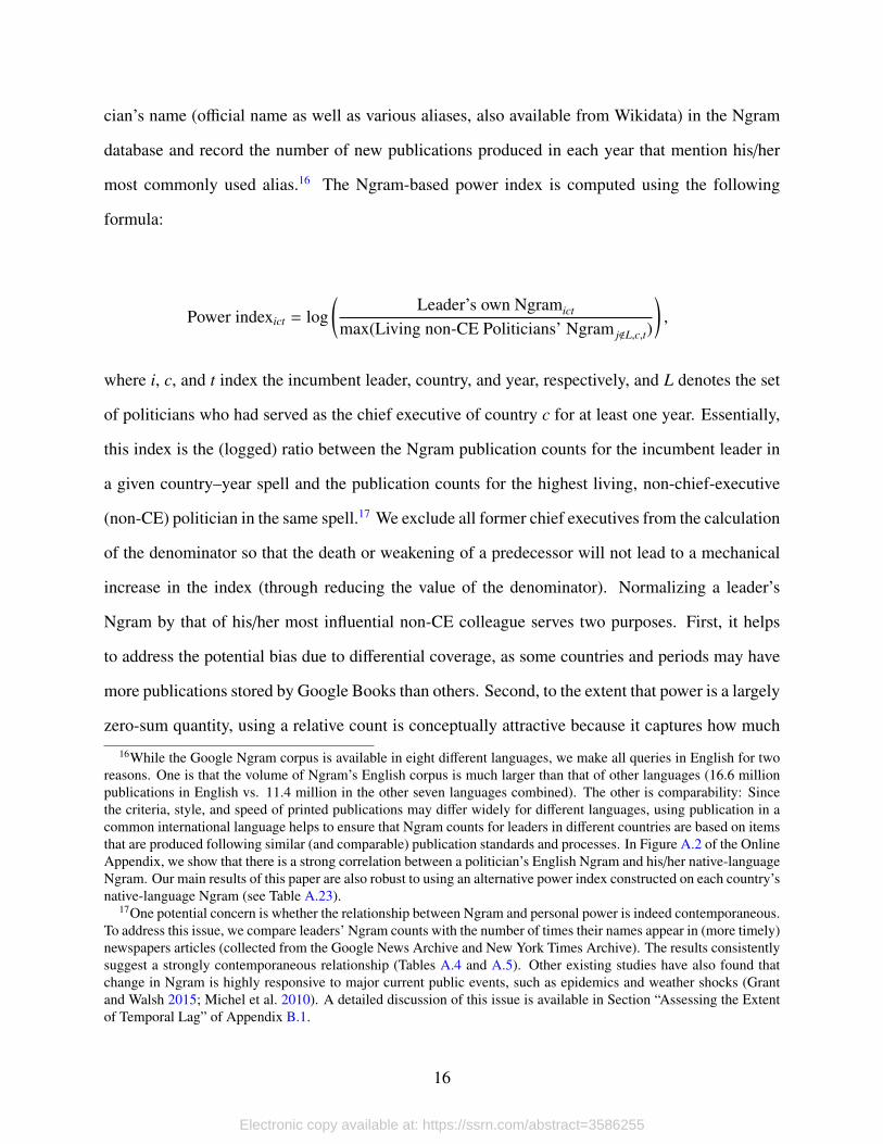
most commonly used alias.16 The Ngram-based power index is computed using the following

formula:

Power indexict = log(

Leader’s own Ngramict

max(Living non-CE Politicians’ Ngram j<L,c,t)

),

where i, c, and t index the incumbent leader, country, and year, respectively, and L denotes the set

of politicians who had served as the chief executive of country c for at least one year. Essentially,

this index is the (logged) ratio between the Ngram publication counts for the incumbent leader in

a given country–year spell and the publication counts for the highest living, non-chief-executive

(non-CE) politician in the same spell.17 We exclude all former chief executives from the calculation

of the denominator so that the death or weakening of a predecessor will not lead to a mechanical

increase in the index (through reducing the value of the denominator). Normalizing a leader’s

Ngram by that of his/her most influential non-CE colleague serves two purposes. First, it helps

to address the potential bias due to differential coverage, as some countries and periods may have

more publications stored by Google Books than others. Second, to the extent that power is a largely

zero-sum quantity, using a relative count is conceptually attractive because it captures how much

16While the Google Ngram corpus is available in eight different languages, we make all queries in English for tworeasons. One is that the volume of Ngram’s English corpus is much larger than that of other languages (16.6 millionpublications in English vs. 11.4 million in the other seven languages combined). The other is comparability: Sincethe criteria, style, and speed of printed publications may differ widely for different languages, using publication in acommon international language helps to ensure that Ngram counts for leaders in different countries are based on itemsthat are produced following similar (and comparable) publication standards and processes. In Figure A.2 of the OnlineAppendix, we show that there is a strong correlation between a politician’s English Ngram and his/her native-languageNgram. Our main results of this paper are also robust to using an alternative power index constructed on each country’snative-language Ngram (see Table A.23).

17One potential concern is whether the relationship between Ngram and personal power is indeed contemporaneous.To address this issue, we compare leaders’ Ngram counts with the number of times their names appear in (more timely)newspapers articles (collected from the Google News Archive and New York Times Archive). The results consistentlysuggest a strongly contemporaneous relationship (Tables A.4 and A.5). Other existing studies have also found thatchange in Ngram is highly responsive to major current public events, such as epidemics and weather shocks (Grantand Walsh 2015; Michel et al. 2010). A detailed discussion of this issue is available in Section “Assessing the Extentof Temporal Lag” of Appendix B.1.

16


attention a top leader receives from publications relative to his/her colleagues. The identities of

the non-CE politicians whose Ngrams are used as the denominator are quite diverse, but typically

belong to one of the following groups: (1) the president in a parliamentary system or the prime

minister in a semi-presidential system, (2) vice presidents or prime ministers, (3) cabinet ministers,

(4) members of the legislature, (5) governors of major states or provinces, or (6) other authoritative

figures such as kings, sultans, or religious leaders (see Figures A.5 and A.6 for details). The

average ratio between the chief executive’s Ngram and the highest non-CE figure’s Ngram is 3.1

(logged ratio = 1.13) in our non-regime-founder sample, with a standard deviation of 5.4.

We conduct a number of validation tests to evaluate the quality of our measure against existing

data and variables. In the interest of space, we leave most of the details to Appendix C, but

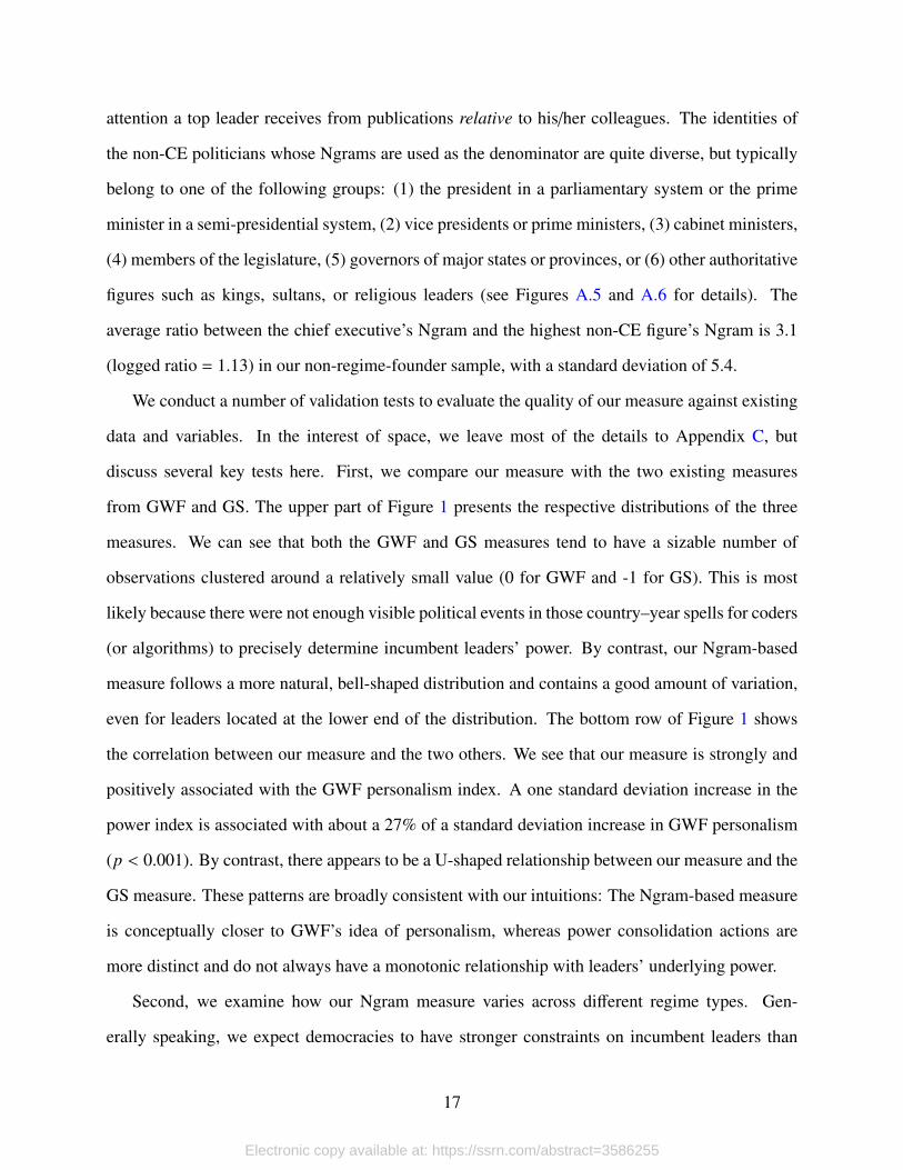
discuss several key tests here. First, we compare our measure with the two existing measures

from GWF and GS. The upper part of Figure 1 presents the respective distributions of the three

measures. We can see that both the GWF and GS measures tend to have a sizable number of

observations clustered around a relatively small value (0 for GWF and -1 for GS). This is most

likely because there were not enough visible political events in those country–year spells for coders

(or algorithms) to precisely determine incumbent leaders’ power. By contrast, our Ngram-based

measure follows a more natural, bell-shaped distribution and contains a good amount of variation,

even for leaders located at the lower end of the distribution. The bottom row of Figure 1 shows

the correlation between our measure and the two others. We see that our measure is strongly and

positively associated with the GWF personalism index. A one standard deviation increase in the

power index is associated with about a 27% of a standard deviation increase in GWF personalism

(p < 0.001). By contrast, there appears to be a U-shaped relationship between our measure and the

GS measure. These patterns are broadly consistent with our intuitions: The Ngram-based measure

is conceptually closer to GWF’s idea of personalism, whereas power consolidation actions are

more distinct and do not always have a monotonic relationship with leaders’ underlying power.

Second, we examine how our Ngram measure varies across different regime types. Gen-

erally speaking, we expect democracies to have stronger constraints on incumbent leaders than

17


non-democracies. Within non-democracies, Geddes (2003) suggests that military and party-based

regimes may have a more collectivist style in exercising power than personalist regimes. In the

bottom row of Figure 1, we plot the average power index of national leaders by the Polity score

(Marshall, Gurr, and Jaggers 2018) and Geddes’ (2003) autocratic regime classification. We see

that as countries become more democratic, the power index of their chief executives becomes

smaller. We also see that top leaders in military and party-based regimes on average have lower

power index than those in monarchies and personalist regimes. These patterns are consistent with

the conventional view of how the levels of power concentration should vary across regime types.

In Appendix C, we use several qualitative examples to illustrate how our Ngram measure cap-

tures the over-time variations in leaders’ power for selected countries and compare it with other

measures (Section C.1). We also report additional validation tests using both cross-country vari-

ables and within-country data from major autocratic regimes in Africa, Asia, Europe, and Latin

America. We find strong relationships between our measure and a number of commonly used

proxies for political power, including the seniority of formal positions (Section C.2), the length of

political leaders’ tenure (Section C.3), candidates’ vote margins in competitive elections (Section

C.4), expert assessment of politicians’ power (Section C.5), the network centrality of political elites

(Section C.6), and the size of senior leaders’ ethnic or factional coalitions (Section C.7). The fact

that our measure tracks closely with power proxies from a variety of settings gives us confidence

in its utility as a general indicator of leaders’ power in cross-country analysis.

18


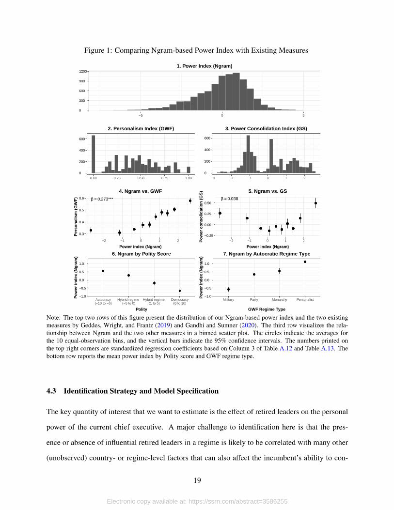
Figure 1: Comparing Ngram-based Power Index with Existing Measures

0

300

600

900

1200

−5 0 5

1. Power Index (Ngram)

0

200

400

600

0.00 0.25 0.50 0.75 1.00

2. Personalism Index (GWF)

0

200

400

600

−3 −2 −1 0 1 2

3. Power Consolidation Index (GS)

β = 0.273***

0.3

0.4

0.5

0.6

−2 −1 0 1 2

Power index (Ngram)

Per

sona

lism

(G

WF

)

4. Ngram vs. GWFβ = 0.038

−0.25

0.00

0.25

0.50

−2 −1 0 1 2

Power index (Ngram)

Pow

er c

onso

lidat

ion

(GS

)

5. Ngram vs. GS

−1.0

−0.5

0.0

0.5

1.0

Autocracy(−10 to −6)

Hybrid regime (−5 to 0)

Hybrid regime (1 to 5)

Democracy(6 to 10)

Polity

Pow

er in

dex

(Ngr

am)

6. Ngram by Polity Score

−1.0

−0.5

0.0

0.5

1.0

Military Party Monarchy Personalist

GWF Regime Type

Pow

er in

dex

(Ngr

am)

7. Ngram by Autocratic Regime Type

Note: The top two rows of this figure present the distribution of our Ngram-based power index and the two existingmeasures by Geddes, Wright, and Frantz (2019) and Gandhi and Sumner (2020). The third row visualizes the rela-tionship between Ngram and the two other measures in a binned scatter plot. The circles indicate the averages forthe 10 equal-observation bins, and the vertical bars indicate the 95% confidence intervals. The numbers printed onthe top-right corners are standardized regression coefficients based on Column 3 of Table A.12 and Table A.13. Thebottom row reports the mean power index by Polity score and GWF regime type.

4.3 Identification Strategy and Model Specification

The key quantity of interest that we want to estimate is the effect of retired leaders on the personal

power of the current chief executive. A major challenge to identification here is that the pres-

ence or absence of influential retired leaders in a regime is likely to be correlated with many other

(unobserved) country- or regime-level factors that can also affect the incumbent’s ability to con-

19


solidate power. For example, more institutionalized regimes may have both stronger constraints on

incumbents and a larger number of living predecessors due to the presence of established norms

that require leaders to step down after a period of service. Sometimes, leaders who plan to initiate

pre-mortem transitions may also deliberately choose weaker successors who are less threatening

and easier to control. Given that these factors are not all observable, a simple cross-regime or even

cross-leader comparison may yield spurious correlations.

Our main strategy to address this endogeneity problem is to include several different types of

fixed effects in regression models. We can include fixed effects for each unique political regime

within a country, assuming that leaders coming to power under the same regime face a more or

less similar political and institutional environment. A more restrictive approach is to include fixed

effects for every unique incumbent leader. The main advantage of the latter approach is that it

eliminates the confounding influence of all unobserved factors that only vary across individual

leaders but not within each leader. This enables us to make weaker identifying assumptions than

a within-regime design (we discuss these assumptions below). However, a potential drawback of

this approach is that it reduces the effective sample size to only those observations where such

variations exist, and this may raise generalizability concerns. In the analysis presented below, we

use the within-leader design as the preferred specification, but also report results from other models

to evaluate the robustness of our findings.

Our main specification is as follows:

Incumbent powerict = αk

K∑t−k

Incumbent poweri,c,t−k

+ δ Predecessor powerict + Xβ + ηi + τt + εict,

where i, c, and t index individual leader, country, and year, respectively. ηi is the leader fixed effects

that capture heterogeneity across incumbent leaders, and τt is the year fixed effects that capture

common, world-wide shocks to the power index. The dependent variable, Incumbent power, is

the Ngram-based power index. Since power is likely to be path-dependent in nature, we also

20


include lagged dependent variables in the model to capture its persistence over time. A common

concern with including lagged dependent variables in a panel fixed-effects setting is the so-called

Nickell bias (Nickell 1981), which is especially worrisome if the panel has a large number of units

but a relatively short time period. However, since our dataset spans several decades, this issue is

mitigated considerably. As a robustness check, we also run regressions using General Methods

of Moments (GMM) estimators (Arellano and Bond 1991) and obtain largely similar results. The

standard errors in all models are clustered at the country level to account for common unobserved

factors that may affect the power of leaders from the same country.

The key explanatory variable, Predecessor power, is computed as follows:

Predecessor poweri,r,t = log[max

(Power as CE j| j<i,r × I(death year j > t) + 1

)]For the ith (i > 2) incumbent leader in regime r at year t, Power as CE j,r is the average power

index of his/her predecessor j during j’s own tenure as the chief executive.18 We choose to focus

on the predecessor’s past influence because of endogeneity concerns: Compared to a predeces-

sor’s contemporary influence (i.e., at t), his/her past influence is less likely to be affected by the

incumbent’s current power. We also restrict the set of predecessors to those who belong to the

same political regime r with the incumbent for the obvious reason that incumbents are unlikely

to be constrained by predecessors from a rival regime. I(death year j > t) is an indicator function

for whether j is still alive at t. The variable Predecessor power is therefore the logged average

power of the most powerful predecessor if there is one or more retired leaders alive,19 and 0 if all

within-regime predecessors are deceased by time t (i.e., death year j 6 t for all j). In our sample,

about 50% of the country–year spells have at least one living predecessor present, and the average

value of a predecessor’s power is about 0.95.

18We use an unlogged version of the power index and only take log later on the average value.19For example, Singapore’s chief executive Lee Hsien Loong (prime minister) faced two living predecessors in

2005: Lee Kuan Yew and Goh Chok Tong. The average of Lee Kuan Yew’s power index over his tenure (1950–1990)is 4.854, whereas the same figure for Goh is 2.478 (tenure length: 1991–2004). Since Lee Kuan Yew has the highestaverage power index of the two, the predecessor power for Lee Hsien Long in 2005 is log(4.854 + 1) = 1.767.

21


Since the average power index is computed based on each predecessor’s time in the top exec-

utive office, its value does not change for the same predecessor throughout her successor’s entire

tenure.20 The only variation in Predecessor power, therefore, comes from the change in the iden-

tity of the most powerful predecessor, which happens when the predecessor who previously had

the highest average power index passes away. As long as we are willing to assume that the deaths

of retired leaders are largely exogenous events, this design allows us to identify the causal effect

of losing a predecessor on the incumbent’s personal power. A close look at the data suggests that

this assumption is reasonable: The vast majority of predecessors’ deaths in our sample (∼76%)

were due to natural illness, and less than 7% were due to assassinations or other premeditated

plots. As a robustness check, we later rerun our analysis on a sample in which all the variations in

predecessors’ power are caused by natural death only, and our results still hold (see Figure 4).

To provide an intuitive illustration of the variations that we use for identification, Figure 2 plots

the co-variation between the incumbents’ power (red, solid lines) and the power of the most in-

fluential predecessors (black, dashed lines) for a selected group of non-democracies. Each shaded

interval represents an uninterrupted period of reign by one incumbent leader. A quick perusal of

the trends suggests that, overall, incumbents’ current power does seem to be negatively correlated

with their predecessors’ past influence, both across and within administrations: When an influen-

tial predecessor is present (i.e., the black, dashed line shows a positive value), the power index of

the incumbent tends to be relatively low. The passing of the influential predecessor in the middle of

an incumbent’s tenure is usually associated with a notable subsequent increase in the incumbent’s

power. These visual patterns are consistent with our hypothesis about the role of predecessors as

informal constraints. In the next section, we provide a more systematic test of this relationship

using regression analysis.

20We do recognize that predecessors’ actual power may not stay constant over their successors’ tenure. We presentrobustness checks using time-varying measures of predecessors’ power in Table A.21.

22


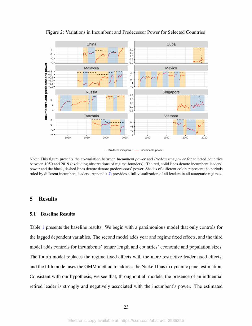
Figure 2: Variations in Incumbent and Predecessor Power for Selected Countries

Tanzania Vietnam

Russia Singapore

Malaysia Mexico

China Cuba

1960 1980 2000 2020 1960 1980 2000 2020

0.00.51.01.52.0

−2−1012

0.6

0.9

1.2

1.5

1.8

−3

−2

−1

0

−2

−1

0

1

−2.0−1.5−1.0−0.50.00.5

−4

−2

0

−4

−2

0

2Incu

mbe

nt's

and

pre

dece

ssor

's p

ower

Predecessor's power Incumbent's power

Note: This figure presents the co-variation between Incumbent power and Predecessor power for selected countriesbetween 1950 and 2019 (excluding observations of regime founders). The red, solid lines denote incumbent leaders’power and the black, dashed lines denote denote predecessors’ power. Shades of different colors represent the periodsruled by different incumbent leaders. Appendix G provides a full visualization of all leaders in all autocratic regimes.

5 Results

5.1 Baseline Results

Table 1 presents the baseline results. We begin with a parsimonious model that only controls for

the lagged dependent variables. The second model adds year and regime fixed effects, and the third

model adds controls for incumbents’ tenure length and countries’ economic and population sizes.

The fourth model replaces the regime fixed effects with the more restrictive leader fixed effects,

and the fifth model uses the GMM method to address the Nickell bias in dynamic panel estimation.

Consistent with our hypothesis, we see that, throughout all models, the presence of an influential

retired leader is strongly and negatively associated with the incumbent’s power. The estimated

23


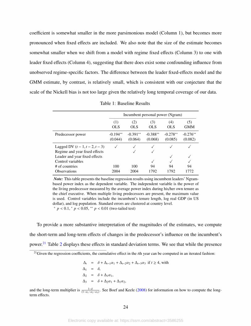
coefficient is somewhat smaller in the more parsimonious model (Column 1), but becomes more

pronounced when fixed effects are included. We also note that the size of the estimate becomes

somewhat smaller when we shift from a model with regime fixed effects (Column 3) to one with

leader fixed effects (Column 4), suggesting that there does exist some confounding influence from

unobserved regime-specific factors. The difference between the leader fixed-effects model and the

GMM estimate, by contrast, is relatively small, which is consistent with our conjecture that the

scale of the Nickell bias is not too large given the relatively long temporal coverage of our data.

Table 1: Baseline Results

Incumbent personal power (Ngram)

(1) (2) (3) (4) (5)OLS OLS OLS OLS GMM

Predecessor power -0.194∗∗ -0.391∗∗ -0.388∗∗ -0.278∗∗ -0.276∗∗

(0.044) (0.064) (0.068) (0.085) (0.082)

Lagged DV (t − 1, t − 2, t − 3) X X X X XRegime and year fixed effects X XLeader and year fixed effects X XControl variables X X X# of countries 100 100 94 94 94Observations 2004 2004 1792 1792 1772

Note: This table presents the baseline regression results using incumbent leaders’ Ngram-based power index as the dependent variable. The independent variable is the power ofthe living predecessor measured by the average power index during his/her own tenure asthe chief executive. When multiple living predecessors are present, the maximum valueis used. Control variables include the incumbent’s tenure length, log real GDP (in USdollar), and log population. Standard errors are clustered at country level.+ p < 0.1, ∗ p < 0.05, ∗∗ p < 0.01 (two-tailed test)

To provide a more substantive interpretation of the magnitudes of the estimates, we compute

the short-term and long-term effects of changes in the predecessor’s influence on the incumbent’s

power.21 Table 2 displays these effects in standard deviation terms. We see that while the presence

21Given the regression coefficients, the cumulative effect in the tth year can be computed in an iterated fashion:

∆t = δ + ∆t−1α1 + ∆t−2α2 + ∆t−3α3 if t ≥ 4, with∆1 = δ,

∆2 = δ + ∆1α1,

∆3 = δ + ∆2α1 + ∆1α2,

and the long-term multiplier is 1−δ(1−α1−α2−α3) . See Boef and Keele (2008) for information on how to compute the long-

term effects.

24


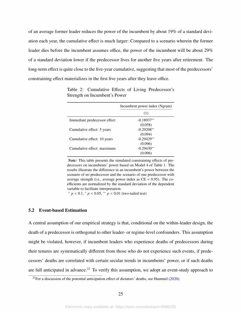
of an average former leader reduces the power of the incumbent by about 19% of a standard devi-

ation each year, the cumulative effect is much larger: Compared to a scenario wherein the former

leader dies before the incumbent assumes office, the power of the incumbent will be about 29%

of a standard deviation lower if the predecessor lives for another five years after retirement. The

long-term effect is quite close to the five-year cumulative, suggesting that most of the predecessors’

constraining effect materializes in the first five years after they leave office.

Table 2: Cumulative Effects of Living Predecessor’sStrength on Incumbent’s Power

Incumbent power index (Ngram)

(1)

Immediate predecessor effect -0.18937∗∗

(0.058)Cumulative effect: 5 years -0.29208∗∗

(0.094)Cumulative effect: 10 years -0.29429∗∗

(0.096)Cumulative effect: maximum -0.29430∗∗

(0.096)

Note: This table presents the simulated constraining effects of pre-decessors on incumbents’ power based on Model 4 of Table 1. Theresults illustrate the difference in an incumbent’s power between thescenario of no predecessor and the scenario of one predecessor withaverage strength (i.e., average power index as CE = 0.95). The co-efficients are normalized by the standard deviation of the dependentvariable to facilitate interpretation.+ p < 0.1, ∗ p < 0.05, ∗∗ p < 0.01 (two-tailed test)

5.2 Event-based Estimation

A central assumption of our empirical strategy is that, conditional on the within-leader design, the

death of a predecessor is orthogonal to other leader- or regime-level confounders. This assumption

might be violated, however, if incumbent leaders who experience deaths of predecessors during

their tenures are systematically different from those who do not experience such events, if prede-

cessors’ deaths are correlated with certain secular trends in incumbents’ power, or if such deaths

are full anticipated in advance.22 To verify this assumption, we adopt an event-study approach to

22For a discussion of the potential anticipation effect of dictators’ deaths, see Hummel (2020).

25


examine the change in incumbent leaders’ power in the few years before and after the death of

their most influential predecessor. Specifically, we estimate the following regression equation:

Incumbent powerict = αk

3∑k=1

Incumbent poweri,c,t−k

+

+4∑τ=−4

δDτ 1{t − Dic = τ} + Xβ + ηi + τt + εict,

where Dic denotes the year in which the event (death of the most influential predecessor) hap-

pened under a given leader i from country c. 1{t − Dic = τ} is an indicator function that assigns 1

to the observation from country c that is τth year relative to the event, and 0 otherwise.

The results from the event-study regression are visualized in Figure 3. We can see that for

incumbent leaders who will soon see the death of their most influential living predecessor, they

do not exhibit significantly different trajectories of power compared to other incumbents (who

either do not have any predecessor at all or face no imminent death of one) prior to the event.

After the passing of the predecessor, however, there is a notable surge in the former group’s power

in the years that immediately follow. This suggests that the constraining effect we observe is

highly specific to the presence or absence of influential predecessors—a finding that testifies to the

credibility of our identification strategy.

26


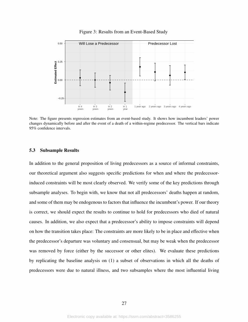
Figure 3: Results from an Event-Based Study

Will Lose a Predecessor Predecessor Lost

−0.25

0.00

0.25

0.50

In 4 years

In 3 years

In 2 years

In 1 year

1 year ago 2 years ago 3 years ago 4 years ago

Est

imat

ed E

ffect

Note: The figure presents regression estimates from an event-based study. It shows how incumbent leaders’ powerchanges dynamically before and after the event of a death of a within-regime predecessor. The vertical bars indicate95% confidence intervals.

5.3 Subsample Results

In addition to the general proposition of living predecessors as a source of informal constraints,

our theoretical argument also suggests specific predictions for when and where the predecessor-

induced constraints will be most clearly observed. We verify some of the key predictions through

subsample analyses. To begin with, we know that not all predecessors’ deaths happen at random,

and some of them may be endogenous to factors that influence the incumbent’s power. If our theory

is correct, we should expect the results to continue to hold for predecessors who died of natural

causes. In addition, we also expect that a predecessor’s ability to impose constraints will depend

on how the transition takes place: The constraints are more likely to be in place and effective when

the predecessor’s departure was voluntary and consensual, but may be weak when the predecessor

was removed by force (either by the successor or other elites). We evaluate these predictions

by replicating the baseline analysis on (1) a subset of observations in which all the deaths of

predecessors were due to natural illness, and two subsamples where the most influential living

27


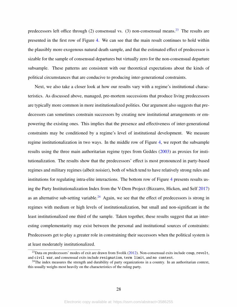
predecessors left office through (2) consensual vs. (3) non-consensual means.23 The results are

presented in the first row of Figure 4. We can see that the main result continues to hold within

the plausibly more exogenous natural death sample, and that the estimated effect of predecessor is

sizable for the sample of consensual departures but virtually zero for the non-consensual departure

subsample. These patterns are consistent with our theoretical expectations about the kinds of

political circumstances that are conducive to producing inter-generational constraints.

Next, we also take a closer look at how our results vary with a regime’s institutional charac-

teristics. As discussed above, managed, pre-mortem successions that produce living predecessors

are typically more common in more institutionalized polities. Our argument also suggests that pre-

decessors can sometimes constrain successors by creating new institutional arrangements or em-

powering the existing ones. This implies that the presence and effectiveness of inter-generational

constraints may be conditioned by a regime’s level of institutional development. We measure

regime institutionalization in two ways. In the middle row of Figure 4, we report the subsample

results using the three main authoritarian regime types from Geddes (2003) as proxies for insti-

tutionalization. The results show that the predecessors’ effect is most pronounced in party-based

regimes and military regimes (albeit noisier), both of which tend to have relatively strong rules and

institutions for regulating intra-elite interactions. The bottom row of Figure 4 presents results us-

ing the Party Institutionalization Index from the V-Dem Project (Bizzarro, Hicken, and Self 2017)

as an alternative sub-setting variable.24 Again, we see that the effect of predecessors is strong in

regimes with medium or high levels of institutionalization, but small and non-significant in the

least institutionalized one third of the sample. Taken together, these results suggest that an inter-

esting complementarity may exist between the personal and institutional sources of constraints:

Predecessors get to play a greater role in constraining their successors when the political system is

at least moderately institutionalized.

23Data on predecessors’ modes of exit are drawn from Svolik (2012). Non-consensual exits include coup, revolt,and civil war, and consensual exits include resignation, term limit, and no contest.

24The index measures the strength and durability of party organizations in a country. In an authoritarian context,this usually weighs most heavily on the characteristics of the ruling party.

28


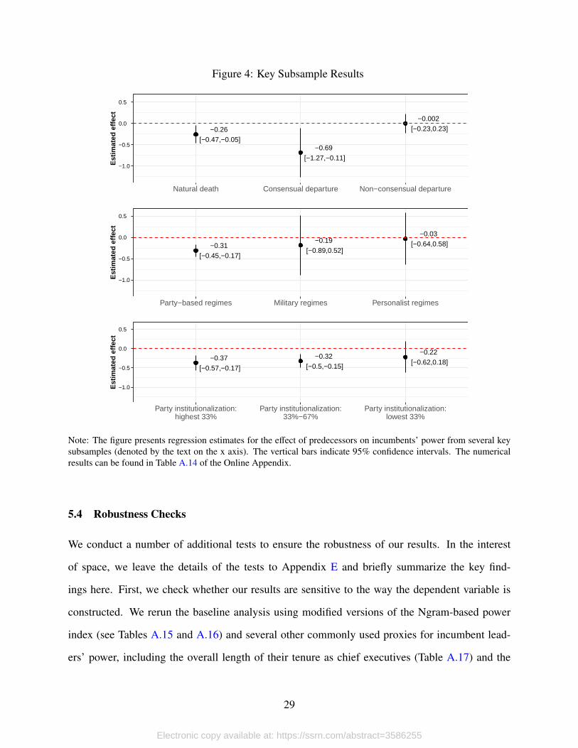
Figure 4: Key Subsample Results

−0.26 [−0.47,−0.05]

−0.69

[−1.27,−0.11]

−0.002 [−0.23,0.23]

−1.0

−0.5

0.0

0.5

Natural death Consensual departure Non−consensual departure

Est

imat

ed e

ffect

−0.31

[−0.45,−0.17]

−0.19 [−0.89,0.52]

−0.03

[−0.64,0.58]

−1.0

−0.5

0.0

0.5

Party−based regimes Military regimes Personalist regimes

Est

imat

ed e

ffect

−0.37

[−0.57,−0.17]

−0.32 [−0.5,−0.15]

−0.22 [−0.62,0.18]

−1.0

−0.5

0.0

0.5

Party institutionalization:highest 33%

Party institutionalization:33%−67%

Party institutionalization:lowest 33%

Est

imat

ed e

ffect

Note: The figure presents regression estimates for the effect of predecessors on incumbents’ power from several keysubsamples (denoted by the text on the x axis). The vertical bars indicate 95% confidence intervals. The numericalresults can be found in Table A.14 of the Online Appendix.

5.4 Robustness Checks

We conduct a number of additional tests to ensure the robustness of our results. In the interest

of space, we leave the details of the tests to Appendix E and briefly summarize the key find-

ings here. First, we check whether our results are sensitive to the way the dependent variable is

constructed. We rerun the baseline analysis using modified versions of the Ngram-based power

index (see Tables A.15 and A.16) and several other commonly used proxies for incumbent lead-

ers’ power, including the overall length of their tenure as chief executives (Table A.17) and the

29


two existing power measures discussed earlier (Tables A.18 and A.19). Most of these alternative

measures yield results very similar to the baseline finding.

We also evaluate the robustness of our independent variable by estimating regressions using

three different measures of the predecessors’ influence: (1) predecessors’ power index based on

the median Ngram as chief executive (as opposed to the mean), (2) a binary indicator for whether

there is any living predecessor from the same regime, and (3) a count variable for the number

of living, within-regime predecessors. The results we obtain are all substantively the same as

the baseline (Tables A.20). In addition, we also introduce two modifications to account for the

possibility that predecessors’ power may change over their successors’ tenure. One modification

is to allow predecessors’ power to decline following some exponential decay functions after they

leave office, and the other is to simply use the current Ngram index of the most influential living

predecessor. Again, our main findings turn out to be highly robust to these modifications (Table

A.21).

Since the operationalization of the definition of authoritarian regimes sometimes varies across

datasets, one concern is that the results may be driven by our sample choice. To address this

concern, we re-run our main analyses on several alternative authoritarian regime samples, such

as Geddes, Wright, and Frantz (2019) and Cheibub, Gandhi, and Vreeland (2009), and find very

similar results (Tables A.25 and A.26). Moreover, we also try to benchmark our findings with a

placebo test. We construct a similar a power index measure for predecessors who are from the

same country but a different regime. The coefficient for the placebo variable is much smaller in

size compared to the original estimate (Table A.27).

6 Evidence on Mechanism

6.1 Evidence from Sub-measures of Personalism and Institutions

The preceding analysis has shown that in durable autocracies where pre-mortem successions are

being practiced, retired leaders often function as a key informal constraint on the power of in-

30


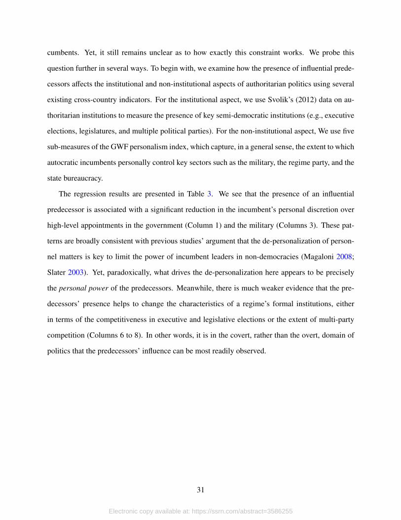
cumbents. Yet, it still remains unclear as to how exactly this constraint works. We probe this

question further in several ways. To begin with, we examine how the presence of influential prede-

cessors affects the institutional and non-institutional aspects of authoritarian politics using several

existing cross-country indicators. For the institutional aspect, we use Svolik’s (2012) data on au-

thoritarian institutions to measure the presence of key semi-democratic institutions (e.g., executive

elections, legislatures, and multiple political parties). For the non-institutional aspect, We use five

sub-measures of the GWF personalism index, which capture, in a general sense, the extent to which

autocratic incumbents personally control key sectors such as the military, the regime party, and the

state bureaucracy.

The regression results are presented in Table 3. We see that the presence of an influential

predecessor is associated with a significant reduction in the incumbent’s personal discretion over

high-level appointments in the government (Column 1) and the military (Columns 3). These pat-

terns are broadly consistent with previous studies’ argument that the de-personalization of person-

nel matters is key to limit the power of incumbent leaders in non-democracies (Magaloni 2008;

Slater 2003). Yet, paradoxically, what drives the de-personalization here appears to be precisely

the personal power of the predecessors. Meanwhile, there is much weaker evidence that the pre-

decessors’ presence helps to change the characteristics of a regime’s formal institutions, either

in terms of the competitiveness in executive and legislative elections or the extent of multi-party

competition (Columns 6 to 8). In other words, it is in the covert, rather than the overt, domain of

politics that the predecessors’ influence can be most readily observed.

31


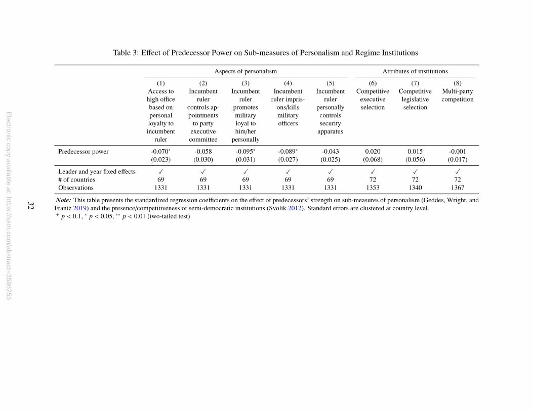
Table 3: Effect of Predecessor Power on Sub-measures of Personalism and Regime Institutions

Aspects of personalism Attributes of institutions

(1) (2) (3) (4) (5) (6) (7) (8)Access tohigh officebased onpersonalloyalty toincumbent

ruler

Incumbentruler

controls ap-pointments

to partyexecutivecommittee

Incumbentruler

promotesmilitaryloyal tohim/her

personally

Incumbentruler impris-

ons/killsmilitaryofficers

Incumbentruler

personallycontrolssecurity

apparatus

Competitiveexecutiveselection

Competitivelegislativeselection

Multi-partycompetition

Predecessor power -0.070∗ -0.058 -0.095∗ -0.089∗ -0.043 0.020 0.015 -0.001(0.023) (0.030) (0.031) (0.027) (0.025) (0.068) (0.056) (0.017)

Leader and year fixed effects X X X X X X X X# of countries 69 69 69 69 69 72 72 72Observations 1331 1331 1331 1331 1331 1353 1340 1367

Note: This table presents the standardized regression coefficients on the effect of predecessors’ strength on sub-measures of personalism (Geddes, Wright, andFrantz 2019) and the presence/competitiveness of semi-democratic institutions (Svolik 2012). Standard errors are clustered at country level.+ p < 0.1, ∗ p < 0.05, ∗∗ p < 0.01 (two-tailed test)

32

Electronic copy available at: https://ssrn.com

/abstract=3586255

6.2 Evidence from Cabinet Appointments

In addition to showing a general pattern with broad-stroke indicators, the highly granular nature

of our Ngram-based measure also enables us to go a step further in unpacking the internal power

dynamics associated with inter-generational constraints. Specifically, since similar Ngram name

counts can in theory be obtained for every politician in a regime, we can go beyond current and for-

mer top leaders and examine how this constraint affects the power distribution among a broader set

of political elites. To do so, we make use of the recently published WhoGov dataset (Nyrup and

Bramwell 2020), which provides a comprehensive collection of cabinet ministers for 177 coun-

tries between 1966 and 2016. Research on authoritarian cabinets suggests that they are important

venues for incumbent autocrats to form ruling coalitions and co-opt potential rivals (Arriola 2009).

Cabinet seats provide elites with access to state resources and influence over government policies;

in some cases, cabinet members also form the critical candidate pool from which a regime’s future

top leaders will be selected. For former leaders, one way for them to retain power over key policies

and personnel matters during retirement is thus to maintain a critical mass of allies and followers

in high-profile cabinet posts. This means that a closer look at cabinet appointments is likely to

provide important insights into how inter-generational checks and balances actually work.

We match the WhoGov dataset with our autocratic regime sample and run the same algorithm

to construct an Ngram-based power index for each cabinet minister based on the number of pub-

lications that mention his/her name in a given year. We then compute the average power index

separately for two groups of cabinet members: (1) those who are first appointed to a cabinet posi-

tion by the incumbent leader (Average Ngram of Incumbents’ Appointees) and (2) those who have

been previously appointed to the cabinet by the incumbent’s within-regime predecessors (Average

Ngram of Predecessors’ Appointees).25 We use the same baseline model (Column 4 of Table 1) to

estimate how predecessors’ power affects these patterns of cabinet appointments.

25For country–year spells where no cabinet member is appointed by predecessors, we treat the average Ngramfor predecessors’ appointees as 0. A similar procedure is used to deal with the (rarer) cases where there is no newappointee by the incumbent leader. The general patterns of our results are robust to simply treating such observationsas missing.

33


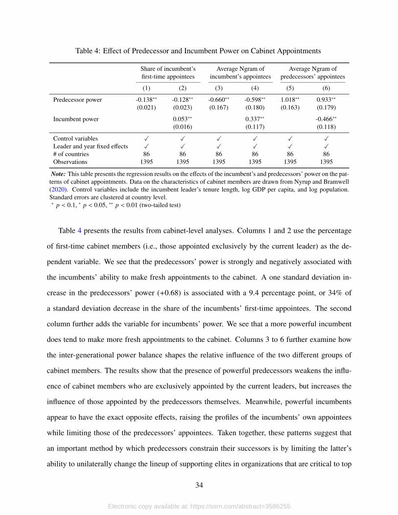
Table 4: Effect of Predecessor and Incumbent Power on Cabinet Appointments

Share of incumbent’sfirst-time appointees

Average Ngram ofincumbent’s appointees

Average Ngram ofpredecessors’ appointees

(1) (2) (3) (4) (5) (6)

Predecessor power -0.138∗∗ -0.128∗∗ -0.660∗∗ -0.598∗∗ 1.018∗∗ 0.933∗∗

(0.021) (0.023) (0.167) (0.180) (0.163) (0.179)

Incumbent power 0.053∗∗ 0.337∗∗ -0.466∗∗

(0.016) (0.117) (0.118)

Control variables X X X X X XLeader and year fixed effects X X X X X X# of countries 86 86 86 86 86 86Observations 1395 1395 1395 1395 1395 1395

Note: This table presents the regression results on the effects of the incumbent’s and predecessors’ power on the pat-terns of cabinet appointments. Data on the characteristics of cabinet members are drawn from Nyrup and Bramwell(2020). Control variables include the incumbent leader’s tenure length, log GDP per capita, and log population.Standard errors are clustered at country level.+ p < 0.1, ∗ p < 0.05, ∗∗ p < 0.01 (two-tailed test)

Table 4 presents the results from cabinet-level analyses. Columns 1 and 2 use the percentage

of first-time cabinet members (i.e., those appointed exclusively by the current leader) as the de-

pendent variable. We see that the predecessors’ power is strongly and negatively associated with

the incumbents’ ability to make fresh appointments to the cabinet. A one standard deviation in-

crease in the predecessors’ power (+0.68) is associated with a 9.4 percentage point, or 34% of

a standard deviation decrease in the share of the incumbents’ first-time appointees. The second

column further adds the variable for incumbents’ power. We see that a more powerful incumbent

does tend to make more fresh appointments to the cabinet. Columns 3 to 6 further examine how

the inter-generational power balance shapes the relative influence of the two different groups of

cabinet members. The results show that the presence of powerful predecessors weakens the influ-

ence of cabinet members who are exclusively appointed by the current leaders, but increases the

influence of those appointed by the predecessors themselves. Meanwhile, powerful incumbents

appear to have the exact opposite effects, raising the profiles of the incumbents’ own appointees

while limiting those of the predecessors’ appointees. Taken together, these patterns suggest that

an important method by which predecessors constrain their successors is by limiting the latter’s

ability to unilaterally change the lineup of supporting elites in organizations that are critical to top

34


leaders’ effective exercise of power.

7 Conclusion

The allocation and contestation of power lie at the heart of elite politics. While much of the ex-

isting literature on authoritarian power politics focuses on institutions, we study how informal,

personalized constraints affect incumbent autocrats’ ability to consolidate power. We demonstrate

that the constraints posed by retired leaders have a discernible negative effect on incumbent lead-

ers’ power, and that the relaxation of such constraints following a predecessor’s death gives the

incumbent an opportunity to expand personal influence. We also provide suggestive evidence on

how this constraint works: It works less by altering the formal and conspicuous aspects of polit-

ical institutions and more by limiting successors’ discretion over the subtle yet crucial domain of

personnel control.

Although the specific inter-generational arrangement that we study here may not necessarily

be present in all autocracies, the central insight that effective constraints on power holders ulti-

mately requires others to hold a commensurate level of power is relevant to a broad set of regimes.

According to the study by Barros (2002), for example, even in a seemingly personalist regime

like Chile under Augusto Pinochet, powerful generals from other branches of the military acted as

key informal checks on Pinochet’s power, and their influence helped to create an effective constitu-

tional framework that paved the way for the subsequent democratic transition. These findings serve

as a cautionary note for the rapidly growing body of literature on authoritarian institutions (Boix

and Svolik 2013; Brownlee 2007a; Gandhi 2008; Magaloni 2008): To the extent that formal in-

stitutions are often deeply intertwined with, and endogenous to, political maneuvering undertaken

by powerful political actors, one needs to be extremely careful when making inferences about the

independent effect of institutions (Cheibub, Przeworski, and Saiegh 2004; Pepinsky 2014). As our

study suggests, institutions sometimes emerge in tandem with the need to cope with succession

challenges, and the effectiveness of institutions as a form of executive constraint depends crucially

on the informal political clout of retired leaders. Ignoring this hidden dimension can lead us to

35


overstate the institutions’ actual ability to constrain incumbents.

This study also has implications for understanding the interplay between authoritarian leaders’

personal power and regime institutionalization. The prevailing view in the literature is that per-

sonalism is antithetical to building strong and robust political institutions (Geddes, Wright, and

Frantz 2019; Levitsky and Ziblatt 2018). Prominent recent studies have similarly argued that weak

leaders are more likely to pursue the strategy of institutionalization as a way of making credible

commitments to other elites (Meng 2020). Our findings, however, suggest a more nuanced and

dynamic interpretation: In some cases, powerful leaders may in fact be a blessing for building

binding institutions if the political exigencies give them the right incentives. As illustrated by the

case of leadership succession, departing leaders who are concerned with protecting their interests

and legacies in retirement may want to put in place strong institutions that will tie the hands of their

successors (rather than themselves). Those with greater personal power are more likely to succeed

because they have greater capacity to defend and enforce nascent institutions and cultivate a norm

of institutional compliance among the elites. Systematic explanations of how strong institutions

take root in a regime, therefore, need to take into account the role played by prominent political

figures, such as George Washington in the United States, Chiang Ching-Kuo in Taiwan, and Deng

Xiaoping in China.

Recognizing the importance of the personalistic input to executive constraint also suggests a

different prediction of long-term institutional dynamics. Contrary to the commonly held view that

institution-building is a path-dependent process whereby institutions, once put in place, become

incrementally stronger as time goes on (Pierson 2000), the fact that effective executive constraints

also need support from strong individuals suggests that strengthening institutional constraints in

the short run may paradoxically sow the seeds for de-institutionalization in the long run: When the

constraints over prior leaders are too strong, those leaders may no longer be able to accumulate

enough power to effectively check their own successors. Therefore, instead of being on a unidirec-

tional path of progression, the rise and fall of institutions may be a cyclical phenomenon over the

long historical duree.

36


Future research can extend this study in at least two ways. First, researchers can further ex-

plore how this specific informal constraint that we identity—the presence or absence of former

leaders—affects incumbent leaders’ behaviors in areas other than power consolidation, such as

policy directions, economic performance, or interstate relations. Second, researchers can try to

explore other sources of informal constraints in autocratic systems. While ex-leaders as a form of

informal constraint may be most applicable to relatively institutionalized autocracies, other types

of constraints, such as the breadth and depth of the ruler’s personal networks, the configurations

of the ethnic and regional interests within the ruling elites, and the relative influence of political

leaders vis-a-vis prominent military, business, and religious figures, may play a greater role in

less institutionalized settings. A better understanding of how those constraints work will shed im-

portant light on both the nature of autocratic power and what limits it in the absence of binding

institutions.

References

Acemoglu, Daron, Georgy Egorov, and Konstantin Sonin. 2008. “Coalition Formation in Non-

Democracies.” The Review of Economic Studies 75 (4): 987–1009.

Albertus, Michael, and Victor Menaldo. 2012. “Dictators as founding fathers? The role of consti-

tutions under autocracy.” Economics & Politics 24 (3): 279–306.

Arellano, Manuel, and Stephen Bond. 1991. “Some Tests of Specification for Panel Data: Monte

Carlo Evidence and an Application to Employment Equations.” The Review of Economic Stud-

ies 58 (2): 277–297.

Arriola, Leonardo R. 2009. “Patronage and Political Stability in Africa.” Comparative Political

Studies 42 (10): 1339–1362.

Ban, Pamela, et al. 2018. “How Newspapers Reveal Political Power.” Online First, Political Science

Research and Methods: 1–18.

37


Barros, Robert. 2002. Constitutionalism and Dictatorship : Pinochet, the Junta, and the 1980 Con-

stitution. Cambridge, UK New York: Cambridge University Press.

Baturo, Alexander. 2014. Democracy, Dictatorship, and Term Limits. University of Michigan

Press.

Bizzarro, Fernando, Allen Hicken, and Darin Self. 2017. The V-Dem Party Institutionalization In-

dex: A New Global Indicator (1900–2015). University of Gothenburg, Varieties of Democracy

Institute, Gothenburg, Sweden. https://bit.ly/3fLEbR9.

Blaydes, Lisa. 2010. Elections and Distributive Politics in Mubarak’s Egypt. Cambridge University

Press.

Boef, Suzanna De, and Luke Keele. 2008. “Taking Time Seriously.” American Journal of Political

Science 52 (1): 184–200.

Boix, Carles, and Milan Svolik. 2013. “The foundations of limited authoritarian government: In-

stitutions, commitment, and power-sharing in dictatorships.” The Journal of Politics 75 (2):

300–316.

Brownlee, Jason. 2007a. Authoritarianism in an Age of Democratization. Cambridge University

Press.

— . 2007b. “Hereditary Succession in Modern Autocracies.” World Politics 59 (4): 595–628.

Bueno de Mesquita, Bruce, et al. 2003. The Logic of Political Survival. MIT Press.

Bunce, Valerie. 2014. Do New Leaders Make a Difference?: Executive Succession and Public

Policy Under Capitalism and Socialism. Princeton Legacy Library. Princeton University Press.

Burling, Robbins. 1974. The Passage of Power: Studies in Political Succession. New York: Aca-

demic Press.

Cheibub, Jose Antonio, Jennifer Gandhi, and James Raymond Vreeland. 2009. “Democracy and

Dictatorship Revisited.” Public Choice 143 (1-2): 67–101.

38


https://bit.ly/3fLEbR9

Cheibub, Jose Antonio, Adam Przeworski, and Sebastian M. Saiegh. 2004. “Government Coali-

tions and Legislative Success under Presidentialism and Parliamentarism.” British Journal of

Political Science 34 (4): 565–587.

Chen, Ting, and Ji Yeon Hong. 2020. “Rivals within: Political Factions, Loyalty, and Elite Com-

petition under Authoritarianism.” Political Science Research and Methods: 1–16.

Chin, James. 2015. “A Decade Later: The Lasting Shadow of Mahathir.” In Malaysia Post-Mahathir:

A Decade of Change, ed. by James Chin and Joern Dosch. Singapore: Marshall Cavendish In-

ternational.

Colgan, Jeff D., and Jessica L.P. Weeks. 2014. “Revolution, Personalist Dictatorships, and Interna-

tional Conflict.” International Organization 69 (1): 163–194.

Dittmer, Lowell. 1978. “Bases of Power in Chinese Politics: A Theory and an Analysis of the Fall

of the ”Gang of Four”.” World Politics 31 (1): 26–60.

— . 2003. “Chinese Factional Politics Under Jiang Zemin.” Journal of East Asian Studies 3 (1):

97–128.

Fischer, Mary. 1989. Nicolae Ceausescu : A Study in Political Leadership. Boulder: L. Rienner

Publishers.

Frantz, Erica, and Elizabeth A. Stein. 2017. “Countering Coups: Leadership Succession Rules in

Dictatorships.” Comparative Political Studies 50 (7): 935–962.

Frantz, Erica, et al. 2020. “Personalization of Power and Repression in Dictatorships.” The Journal

of Politics 82 (1): 372–377.

Gandhi, Jennifer. 2008. Political Institutions under Dictatorship. Cambridge University Press.

Gandhi, Jennifer, and Ellen Lust-Okar. 2009. “Elections under authoritarianism.” Annual review

of political science 12:403–422.

Gandhi, Jennifer, and Jane Lawrence Sumner. 2020. “Measuring the Consolidation of Power in

Nondemocracies.” The Journal of Politics 82 (4): 1545–1558.

39


Geddes, Barbara. 2003. Paradigms and Sand Castles: Theory Building and Research Design in

Comparative Politics. University of Michigan Press.

Geddes, Barbara, Joseph Wright, and Erica Frantz. 2014. “Autocratic Breakdown and Regime

Transitions: A New Data Set.” Perspectives on Politics 12 (2): 313–331.

— . 2019. How Dictatorships Work. New York: Cambridge University Press.

Gehlbach, Scott, and Philip Keefer. 2011. “Investment without Democracy: Ruling-party Institu-

tionalization and Credible Commitment in Autocracies.” Journal of Comparative Economics

39 (2): 123–139.

— . 2012. “Private Investment and the Institutionalization of Collective Action in Autocracies:

Ruling Parties and Legislatures.” The Journal of Politics 74 (02): 621–635.

Goemans, Henk E., Kristian Skrede Gleditsch, and Giacomo Chiozza. 2009. “Introducing Archi-

gos: A Dataset of Political Leaders.” Journal of Peace Research 46 (2): 269–283.

Grant, Will J., and Erin Walsh. 2015. “Social evidence of a changing climate: Google Ngram data

points to early climate change impact on human society.” Weather 70 (7): 195–197.

Grzymala-Busse, Anna. 2010. “The Best Laid Plans: The Impact of Informal Rules on Formal

Institutions in Transitional Regimes.” Studies in Comparative International Development 45

(3): 311–333.

Helmke, Gretchen, and Steven Levitsky. 2004. “Informal Institutions and Comparative Politics: A

Research Agenda.” Perspectives on Politics 2 (4): 725–740.

Hummel, Sarah. 2020. “Leader age, death, and political liberalization in dictatorships.” The Jour-

nal of Politics 82 (3): 981–995.

Huntington, Samuel P., and Clement Henry Moore, eds. 1970. Authoritarian Politics in Modern

Society: The Dynamics of Established One-Party Systems. Basic Books.

Ilkhamov, Alisher. 2007. “Neopatrimonialism, Interest Groups and Patronage Networks: The Im-

passes of the Governance System in Uzbekistan.” Central Asian Survey 26 (1): 65–84.

40


Jaros, Kyle, and Jennifer Pan. 2017. “China’s Newsmakers: Official Media Coverage and Political

Shifts in the Xi Jinping Era.” The China Quarterly 233:111–136.

Kokkonen, Andrej, and Anders Sundell. 2014. “Delivering Stability: Primogeniture and Autocratic

Survival in European Monarchies 1000-1800.” American Political Science Review 108 (02):

438–453.

Kroeger, Alex. 2018. “Dominant Party Rule, Elections, and Cabinet Instability in African Autoc-

racies.” British Journal of Political Science: 1–23.

Kuhn, Robert.Lawrence. 2004. The Man who Changed China: The Life and Legacy of Jiang Zemin.

Crown Publishers.

Kurrild-Klitgaard, Peter. 2000. “The Constitutional Economics of Autocratic Succession.” Public

Choice 103 (1-2): 63–84.

Levitsky, Steven, and Marıa Victoria Murillo. 2009. “Variation in Institutional Strength.” Annual

Review of Political Science 12 (1): 115–133.

Levitsky, Steven, and Daniel Ziblatt. 2018. How Democracies Die. Crown/Archetype.

Li, Cheng. 2016. Chinese Politics in the Xi Jinping Era: Reassessing Collective Leadership. Brook-

ings Institution Press.

Luo, Zhaotian, and Arturas Rozenas. 2016. “Ruling the Ruling Coalition: Information Control and

Autocratic Governance.” SSRN Electronic Journal.

Ma, Xiao. 2016. “Term Limits and Authoritarian Power Sharing: Theory and Evidence from

China.” Journal of East Asian Studies 16 (1): 61–85.

Magaloni, Beatriz. 2008. “Credible Power-Sharing and the Longevity of Authoritarian Rule.” Com-

parative Political Studies 41 (4-5): 715–741.

Marshall, Monty, Ted Gurr, and Keith Jaggers. 2018. Polity IV Project: Political Regime Charac-

teristics and Transitions, 1800-2017. Center for Systemic Peace.

41


Mauzy, Diane K., and R. S. Milne. 2002. Singapore Politics Under the People’s Action Party.

Routledge Chapman Hall.

Meng, Anne. 2020. Constraining Dictatorship: From Personalized Rule to Institutionalized Regimes.

Cambridge University Press.

— . 2019. “Ruling Parties in Authoritarian Regimes: Rethinking Institutional Strength.” British

Journal of Political Science: 1–15.

Michel, Jean-Baptiste, et al. 2010. “Quantitative Analysis of Culture Using Millions of Digitized

Books.” Science 331 (6014): 176–182.

Miller, Michael K. 2015. “Elections, Information, and Policy Responsiveness in Autocratic Regimes.”

Comparative Political Studies 48 (6): 691–727.

Myerson, Roger B. 2008. “The Autocrat’s Credibility Problem and Foundations of the Constitu-

tional State.” The American Political Science Review 102 (1): pp. 125–139.

Nickell, Stephen. 1981. “Biases in Dynamic Models with Fixed Effects.” Econometrica 49 (6):

1417–1426.

Nyrup, Jacob, and Stuart Bramwell. 2020. “Who Governs? A New Global Dataset on Members of

Cabinets.” American Political Science Review 114 (4): 1366–1374.

Padgett, John F., and Christopher K. Ansell. 1993. “Robust Action and the Rise of the Medici,

1400-1434.” American Journal of Sociology 98 (6): 1259–1319.

Pepinsky, Thomas. 2014. “The Institutional Turn in Comparative Authoritarianism.” British Jour-

nal of Political Science 44 (03): 631–653.

Pepinsky, Thomas B. 2015. Economic Crises and the Breakdown of Authoritarian Regimes. Cam-

bridge University Press.

Pierson, Paul. 2000. “Increasing Returns, Path Dependence, and the Study of Politics.” The Amer-

ican Political Science Review 94 (2): 251–267.

42


Przeworski, Adam. 2013. Political Institutions and Political Events Data Set. Department of Poli-

tics, New York University.

Reuter, Ora John. 2017. The Origins of Dominant Parties: Building Authoritarian Institutions in

Post-Soviet Russia. Cambridge University Press.

Richey, Sean, and J. Benjamin Taylor. 2019. “Google Books Ngrams and Political Science: Two

Validity Tests for a Novel Data Source.” PS: Political Science & Politics 53 (1): 72–77.

Shea, Daniel M., and Alex Sproveri. 2012. “The Rise and Fall of Nasty Politics in America.” PS:

Political Science & Politics 45 (03): 416–421.

Slater, Dan. 2003. “Iron Cage in an Iron Fist: Authoritarian Institutions and the Personalization of

Power in Malaysia.” Comparative Politics 36 (1): 81–101.

Smith, Peter H. 1991. “Mexico since 1946: Dynamics of an Authoritarian Regime.” In Mexico

since Independence, ed. by Leslie Bethell, 321–396. Cambridge University Press.

Southall, Roger. 2006. “Troubled Visionary: Nyerere as a Former President.” In Legacies of Power

: Leadership Change and Former Presidents in African Politics, ed. by Roger Southall and

Henning Melber, 233–255. Uppsala, Sweden: The Nordic Africa Institute.

Spearman, Diana. 1939. Modern Dictatorship. Columbia University Press.

Svolik, Milan. 2012. The Politics of Authoritarian Rule. Cambridge University Press.

Svolik, Milan W. 2009. “Power Sharing and Leadership Dynamics in Authoritarian Regimes.”

American Journal of Political Science 53 (2): 477–494.

Throup, David, and Charles Hornsby. 1998. Multi-party Politics in Kenya : The Kenyatta & Moi

States & the Triumph of the System in the 1992 Election. Oxford: Ohio University Press.

Treisman, Daniel. 2015. “Income, Democracy, and Leader Turnover.” American Journal of Politi-

cal Science 59 (4): 927–942.

Tullock, Gordon. 1987. Autocracy. Springer Science & Business Media.

43


Vogel, Ezra. 2013. Deng Xiaoping and the Transformation of China. Belknap Press of Harvard

University Press.

Vrandecic, Denny, and Markus Krotzsch. 2014. “Wikidata: A Free Collaborative Knowledgebase.”

Commun. ACM (New York, NY, USA) 57 (10): 78–85.

Weeks, Jessica L. 2012. “Strongmen and Straw Men: Authoritarian Regimes and the Initiation of

International Conflict.” American Political Science Review 106 (02): 326–347.

Wright, Joseph. 2008. “Do Authoritarian Institutions Constrain? How Legislatures Affect Eco-

nomic Growth and Investment.” American Journal of Political Science 52 (2): 322–343.

Wright, Joseph, and Abel Escriba-Folch. 2012. “Authoritarian institutions and regime survival:

Transitions to democracy and subsequent autocracy.” British Journal of Political Science 42

(2): 283–309.

Zhang, Yongjing. 2011. “The Successor’s Dilemma in China’s Single Party Political System.”

European Journal of Political Economy 27 (4): 674–680.

44


Online Appendix (Not for Publication) forIn the Shadows of Great Men: Leadership Turnovers and Power Dynamics inAutocracies

A Summary Statistics A-2

B Measuring Personal Power from Google Ngram A-3B.1 Details about Publications Underlying Google Ngram . . . . . . . . . . . . . . . A-4B.2 Construction Procedures . . . . . . . . . . . . . . . . . . . . . . . . . . . . . . . A-9

C Validation Exercises A-14C.1 Examples . . . . . . . . . . . . . . . . . . . . . . . . . . . . . . . . . . . . . . . A-15C.2 Correlation with the Formal Political Hierarchy . . . . . . . . . . . . . . . . . . . A-20C.3 Correlation with Leaders’ Tenure . . . . . . . . . . . . . . . . . . . . . . . . . . . A-22C.4 Correlation with Electoral Outcomes . . . . . . . . . . . . . . . . . . . . . . . . . A-23C.5 Correlation with Expert Rating of Politicians’ Power . . . . . . . . . . . . . . . . A-25C.6 Correlation with Network-based Power of Mexican Elites . . . . . . . . . . . . . . A-26C.7 Ngram and Coalitional Power . . . . . . . . . . . . . . . . . . . . . . . . . . . . A-28C.8 Correlation with Existing Power Measures . . . . . . . . . . . . . . . . . . . . . . A-34

D Numerical Results for Subsample Analyses A-36

E Detailed Results of Robustness Checks A-37E.1 Alternative Dependent Variables . . . . . . . . . . . . . . . . . . . . . . . . . . . A-37E.2 Alternative Independent Variables . . . . . . . . . . . . . . . . . . . . . . . . . . A-41

F Non-Linearity in Predecessors’ Influence on Incumbents A-47

G Visualization of Power Dynamics for All Autocratic Regimes, 1950–2019 A-49

A-1


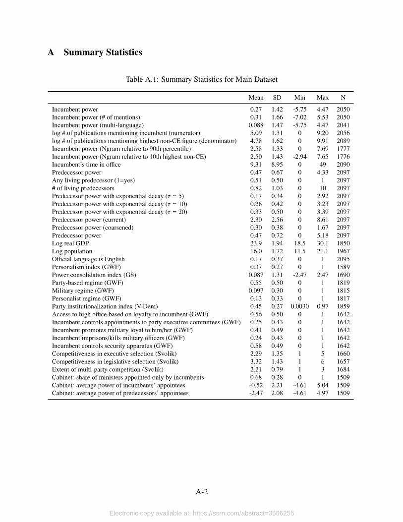
A Summary Statistics

Table A.1: Summary Statistics for Main Dataset

Mean SD Min Max N

Incumbent power 0.27 1.42 -5.75 4.47 2050Incumbent power (# of mentions) 0.31 1.66 -7.02 5.53 2050Incumbent power (multi-language) 0.088 1.47 -5.75 4.47 2041log # of publications mentioning incumbent (numerator) 5.09 1.31 0 9.20 2056log # of publications mentioning highest non-CE figure (denominator) 4.78 1.62 0 9.91 2089Incumbent power (Ngram relative to 90th percentile) 2.58 1.33 0 7.69 1777Incumbent power (Ngram relative to 10th highest non-CE) 2.50 1.43 -2.94 7.65 1776Incumbent’s time in office 9.31 8.95 0 49 2090Predecessor power 0.47 0.67 0 4.33 2097Any living predecessor (1=yes) 0.51 0.50 0 1 2097# of living predecessors 0.82 1.03 0 10 2097Predecessor power with exponential decay (τ = 5) 0.17 0.34 0 2.92 2097Predecessor power with exponential decay (τ = 10) 0.26 0.42 0 3.23 2097Predecessor power with exponential decay (τ = 20) 0.33 0.50 0 3.39 2097Predecessor power (current) 2.30 2.56 0 8.61 2097Predecessor power (coarsened) 0.30 0.38 0 1.67 2097Predecessor power 0.47 0.72 0 5.18 2097Log real GDP 23.9 1.94 18.5 30.1 1850Log population 16.0 1.72 11.5 21.1 1967Official language is English 0.17 0.37 0 1 2095Personalism index (GWF) 0.37 0.27 0 1 1589Power consolidation index (GS) 0.087 1.31 -2.47 2.47 1690Party-based regime (GWF) 0.55 0.50 0 1 1819Military regime (GWF) 0.097 0.30 0 1 1815Personalist regime (GWF) 0.13 0.33 0 1 1817Party institutionalization index (V-Dem) 0.45 0.27 0.0030 0.97 1859Access to high office based on loyalty to incumbent (GWF) 0.56 0.50 0 1 1642Incumbent controls appointments to party executive committees (GWF) 0.25 0.43 0 1 1642Incumbent promotes military loyal to him/her (GWF) 0.41 0.49 0 1 1642Incumbent imprisons/kills military officers (GWF) 0.24 0.43 0 1 1642Incumbent controls security apparatus (GWF) 0.58 0.49 0 1 1642Competitiveness in executive selection (Svolik) 2.29 1.35 1 5 1660Competitiveness in legislative selection (Svolik) 3.32 1.43 1 6 1657Extent of multi-party competition (Svolik) 2.21 0.79 1 3 1684Cabinet: share of ministers appointed only by incumbents 0.68 0.28 0 1 1509Cabinet: average power of incumbents’ appointees -0.52 2.21 -4.61 5.04 1509Cabinet: average power of predecessors’ appointees -2.47 2.08 -4.61 4.97 1509

A-2


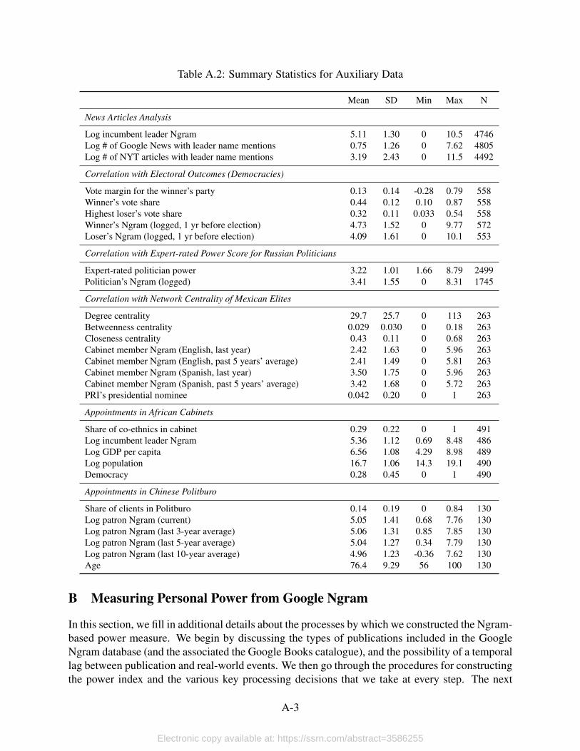
Table A.2: Summary Statistics for Auxiliary Data

Mean SD Min Max N

News Articles Analysis

Log incumbent leader Ngram 5.11 1.30 0 10.5 4746Log # of Google News with leader name mentions 0.75 1.26 0 7.62 4805Log # of NYT articles with leader name mentions 3.19 2.43 0 11.5 4492

Correlation with Electoral Outcomes (Democracies)

Vote margin for the winner’s party 0.13 0.14 -0.28 0.79 558Winner’s vote share 0.44 0.12 0.10 0.87 558Highest loser’s vote share 0.32 0.11 0.033 0.54 558Winner’s Ngram (logged, 1 yr before election) 4.73 1.52 0 9.77 572Loser’s Ngram (logged, 1 yr before election) 4.09 1.61 0 10.1 553

Correlation with Expert-rated Power Score for Russian Politicians

Expert-rated politician power 3.22 1.01 1.66 8.79 2499Politician’s Ngram (logged) 3.41 1.55 0 8.31 1745

Correlation with Network Centrality of Mexican Elites

Degree centrality 29.7 25.7 0 113 263Betweenness centrality 0.029 0.030 0 0.18 263Closeness centrality 0.43 0.11 0 0.68 263Cabinet member Ngram (English, last year) 2.42 1.63 0 5.96 263Cabinet member Ngram (English, past 5 years’ average) 2.41 1.49 0 5.81 263Cabinet member Ngram (Spanish, last year) 3.50 1.75 0 5.96 263Cabinet member Ngram (Spanish, past 5 years’ average) 3.42 1.68 0 5.72 263PRI’s presidential nominee 0.042 0.20 0 1 263

Appointments in African Cabinets

Share of co-ethnics in cabinet 0.29 0.22 0 1 491Log incumbent leader Ngram 5.36 1.12 0.69 8.48 486Log GDP per capita 6.56 1.08 4.29 8.98 489Log population 16.7 1.06 14.3 19.1 490Democracy 0.28 0.45 0 1 490

Appointments in Chinese Politburo

Share of clients in Politburo 0.14 0.19 0 0.84 130Log patron Ngram (current) 5.05 1.41 0.68 7.76 130Log patron Ngram (last 3-year average) 5.06 1.31 0.85 7.85 130Log patron Ngram (last 5-year average) 5.04 1.27 0.34 7.79 130Log patron Ngram (last 10-year average) 4.96 1.23 -0.36 7.62 130Age 76.4 9.29 56 100 130

B Measuring Personal Power from Google Ngram

In this section, we fill in additional details about the processes by which we constructed the Ngram-based power measure. We begin by discussing the types of publications included in the GoogleNgram database (and the associated the Google Books catalogue), and the possibility of a temporallag between publication and real-world events. We then go through the procedures for constructingthe power index and the various key processing decisions that we take at every step. The next

A-3


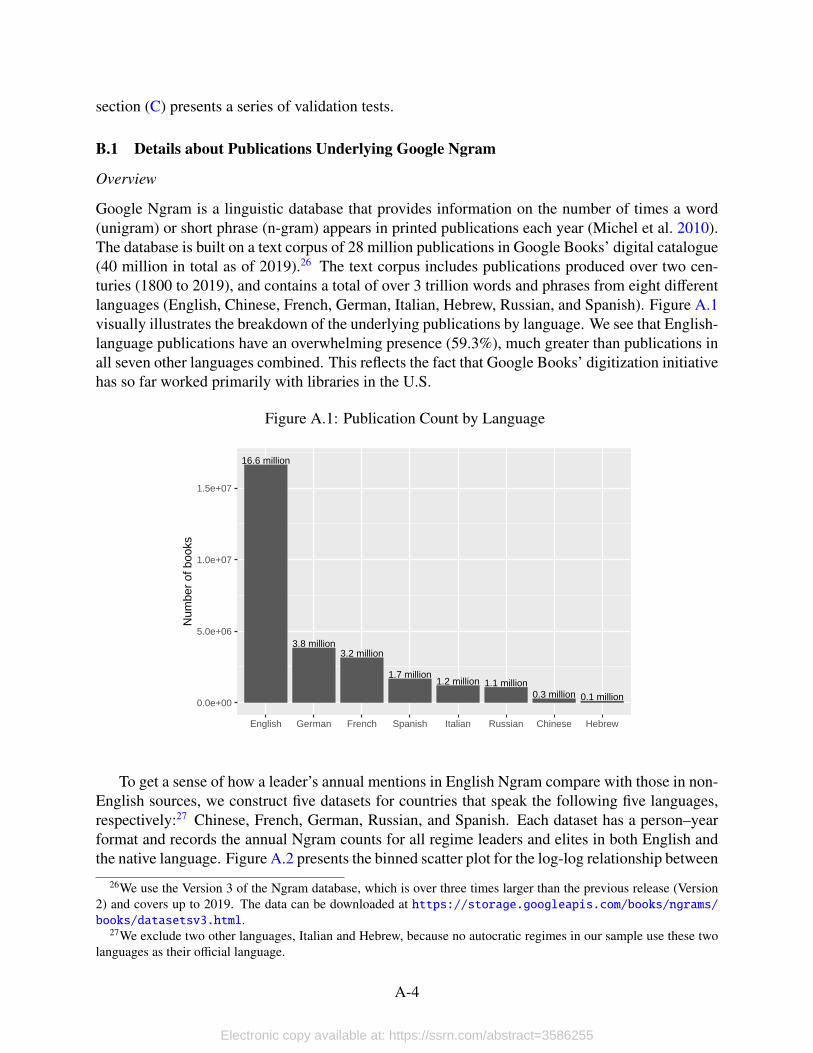
section (C) presents a series of validation tests.

B.1 Details about Publications Underlying Google Ngram

Overview

Google Ngram is a linguistic database that provides information on the number of times a word(unigram) or short phrase (n-gram) appears in printed publications each year (Michel et al. 2010).The database is built on a text corpus of 28 million publications in Google Books’ digital catalogue(40 million in total as of 2019).26 The text corpus includes publications produced over two cen-turies (1800 to 2019), and contains a total of over 3 trillion words and phrases from eight differentlanguages (English, Chinese, French, German, Italian, Hebrew, Russian, and Spanish). Figure A.1visually illustrates the breakdown of the underlying publications by language. We see that English-language publications have an overwhelming presence (59.3%), much greater than publications inall seven other languages combined. This reflects the fact that Google Books’ digitization initiativehas so far worked primarily with libraries in the U.S.

Figure A.1: Publication Count by Language

0.1 million0.3 million1.1 million1.2 million

1.7 million

3.2 million3.8 million

16.6 million

0.0e+00

5.0e+06

1.0e+07

1.5e+07

English German French Spanish Italian Russian Chinese Hebrew

Num

ber

of b

ooks

To get a sense of how a leader’s annual mentions in English Ngram compare with those in non-English sources, we construct five datasets for countries that speak the following five languages,respectively:27 Chinese, French, German, Russian, and Spanish. Each dataset has a person–yearformat and records the annual Ngram counts for all regime leaders and elites in both English andthe native language. Figure A.2 presents the binned scatter plot for the log-log relationship between

26We use the Version 3 of the Ngram database, which is over three times larger than the previous release (Version2) and covers up to 2019. The data can be downloaded at https://storage.googleapis.com/books/ngrams/books/datasetsv3.html.

27We exclude two other languages, Italian and Hebrew, because no autocratic regimes in our sample use these twolanguages as their official language.

A-4


https://storage.googleapis.com/books/ngrams/books/datasetsv3.html

https://storage.googleapis.com/books/ngrams/books/datasetsv3.html

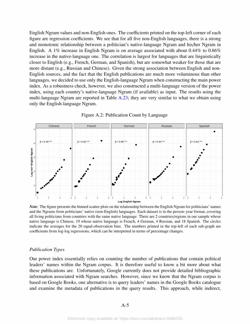
English Ngram values and non-English ones. The coefficients printed on the top-left corner of eachfigure are regression coefficients. We see that for all five non-English languages, there is a strongand monotonic relationship between a politician’s native-language Ngram and his/her Ngram inEnglish. A 1% increase in English Ngram is on average associated with about 0.44% to 0.66%increase in the native-language one. The correlation is largest for languages that are linguisticallycloser to English (e.g., French, German, and Spanish), but are somewhat weaker for those that aremore distant (e.g., Russian and Chinese). Given the strong association between English and non-English sources, and the fact that the English publications are much more voluminous than otherlanguages, we decided to use only the English-language Ngram when constructing the main powerindex. As a robustness check, however, we also constructed a multi-language version of the powerindex, using each country’s native-language Ngram (if available) as input. The results using themulti-language Ngram are reported in Table A.23; they are very similar to what we obtain usingonly the English-language Ngram.

Figure A.2: Publication Count by Language

β = 0.49 *** β = 0.65 *** β = 0.66 *** β = 0.44 *** β = 0.62 ***

Chinese French German Russian Spanish

0 2 4 6 0 2 4 6 0 2 4 6 0 2 4 6 0 2 4 6

1

2

3

4

5

Log English Ngram

Log

non−

Eng

lish

Ngr

am

Note: The figure presents the binned scatter plots on the relationship between the English Ngram for politicians’ namesand the Ngrams from politicians’ native (non-English) languages. Each dataset is in the person–year format, coveringall living politicians from countries with the same native language. There are 2 countries/regions in our sample whosenative language is Chinese, 19 whose native language is French, 4 German, 4 Russian, and 18 Spanish. The circlesindicate the averages for the 20 equal-observation bins. The numbers printed in the top-left of each sub-graph arecoefficients from log-log regressions, which can be interpreted in terms of percentage changes.

Publication Types

Our power index essentially relies on counting the number of publications that contain politicalleaders’ names within the Ngram corpus. It is therefore useful to know a bit more about whatthese publications are. Unfortunately, Google currently does not provide detailed bibliographicinformation associated with Ngram searches. However, since we know that the Ngram corpus isbased on Google Books, one alternative is to query leaders’ names in the Google Books catalogueand examine the metadata of publications in the query results. This approach, while indirect,

A-5


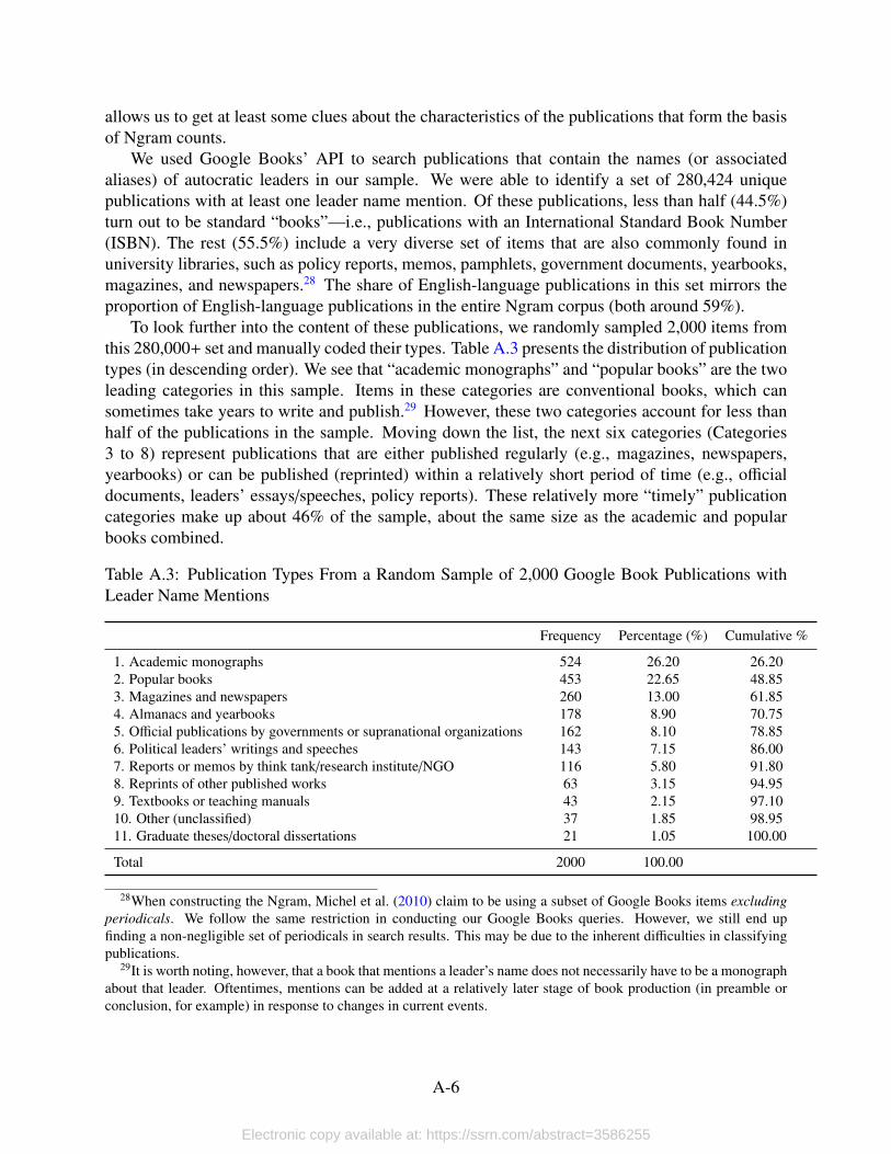
allows us to get at least some clues about the characteristics of the publications that form the basisof Ngram counts.

We used Google Books’ API to search publications that contain the names (or associatedaliases) of autocratic leaders in our sample. We were able to identify a set of 280,424 uniquepublications with at least one leader name mention. Of these publications, less than half (44.5%)turn out to be standard “books”—i.e., publications with an International Standard Book Number(ISBN). The rest (55.5%) include a very diverse set of items that are also commonly found inuniversity libraries, such as policy reports, memos, pamphlets, government documents, yearbooks,magazines, and newspapers.28 The share of English-language publications in this set mirrors theproportion of English-language publications in the entire Ngram corpus (both around 59%).

To look further into the content of these publications, we randomly sampled 2,000 items fromthis 280,000+ set and manually coded their types. Table A.3 presents the distribution of publicationtypes (in descending order). We see that “academic monographs” and “popular books” are the twoleading categories in this sample. Items in these categories are conventional books, which cansometimes take years to write and publish.29 However, these two categories account for less thanhalf of the publications in the sample. Moving down the list, the next six categories (Categories3 to 8) represent publications that are either published regularly (e.g., magazines, newspapers,yearbooks) or can be published (reprinted) within a relatively short period of time (e.g., officialdocuments, leaders’ essays/speeches, policy reports). These relatively more “timely” publicationcategories make up about 46% of the sample, about the same size as the academic and popularbooks combined.

Table A.3: Publication Types From a Random Sample of 2,000 Google Book Publications withLeader Name Mentions

Frequency Percentage (%) Cumulative %

1. Academic monographs 524 26.20 26.202. Popular books 453 22.65 48.853. Magazines and newspapers 260 13.00 61.854. Almanacs and yearbooks 178 8.90 70.755. Official publications by governments or supranational organizations 162 8.10 78.856. Political leaders’ writings and speeches 143 7.15 86.007. Reports or memos by think tank/research institute/NGO 116 5.80 91.808. Reprints of other published works 63 3.15 94.959. Textbooks or teaching manuals 43 2.15 97.1010. Other (unclassified) 37 1.85 98.9511. Graduate theses/doctoral dissertations 21 1.05 100.00

Total 2000 100.00

28When constructing the Ngram, Michel et al. (2010) claim to be using a subset of Google Books items excludingperiodicals. We follow the same restriction in conducting our Google Books queries. However, we still end upfinding a non-negligible set of periodicals in search results. This may be due to the inherent difficulties in classifyingpublications.

29It is worth noting, however, that a book that mentions a leader’s name does not necessarily have to be a monographabout that leader. Oftentimes, mentions can be added at a relatively later stage of book production (in preamble orconclusion, for example) in response to changes in current events.

A-6


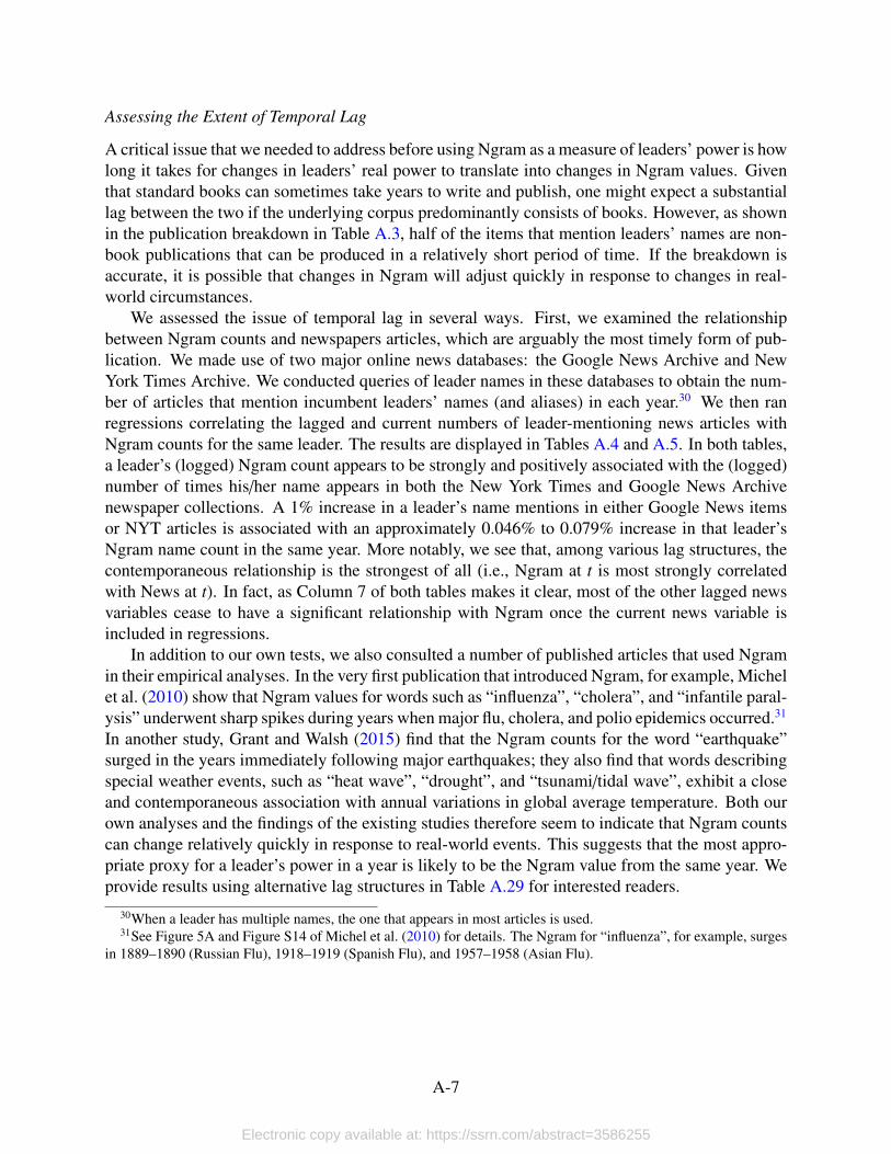
Assessing the Extent of Temporal Lag

A critical issue that we needed to address before using Ngram as a measure of leaders’ power is howlong it takes for changes in leaders’ real power to translate into changes in Ngram values. Giventhat standard books can sometimes take years to write and publish, one might expect a substantiallag between the two if the underlying corpus predominantly consists of books. However, as shownin the publication breakdown in Table A.3, half of the items that mention leaders’ names are non-book publications that can be produced in a relatively short period of time. If the breakdown isaccurate, it is possible that changes in Ngram will adjust quickly in response to changes in real-world circumstances.

We assessed the issue of temporal lag in several ways. First, we examined the relationshipbetween Ngram counts and newspapers articles, which are arguably the most timely form of pub-lication. We made use of two major online news databases: the Google News Archive and NewYork Times Archive. We conducted queries of leader names in these databases to obtain the num-ber of articles that mention incumbent leaders’ names (and aliases) in each year.30 We then ranregressions correlating the lagged and current numbers of leader-mentioning news articles withNgram counts for the same leader. The results are displayed in Tables A.4 and A.5. In both tables,a leader’s (logged) Ngram count appears to be strongly and positively associated with the (logged)number of times his/her name appears in both the New York Times and Google News Archivenewspaper collections. A 1% increase in a leader’s name mentions in either Google News itemsor NYT articles is associated with an approximately 0.046% to 0.079% increase in that leader’sNgram name count in the same year. More notably, we see that, among various lag structures, thecontemporaneous relationship is the strongest of all (i.e., Ngram at t is most strongly correlatedwith News at t). In fact, as Column 7 of both tables makes it clear, most of the other lagged newsvariables cease to have a significant relationship with Ngram once the current news variable isincluded in regressions.

In addition to our own tests, we also consulted a number of published articles that used Ngramin their empirical analyses. In the very first publication that introduced Ngram, for example, Michelet al. (2010) show that Ngram values for words such as “influenza”, “cholera”, and “infantile paral-ysis” underwent sharp spikes during years when major flu, cholera, and polio epidemics occurred.31

In another study, Grant and Walsh (2015) find that the Ngram counts for the word “earthquake”surged in the years immediately following major earthquakes; they also find that words describingspecial weather events, such as “heat wave”, “drought”, and “tsunami/tidal wave”, exhibit a closeand contemporaneous association with annual variations in global average temperature. Both ourown analyses and the findings of the existing studies therefore seem to indicate that Ngram countscan change relatively quickly in response to real-world events. This suggests that the most appro-priate proxy for a leader’s power in a year is likely to be the Ngram value from the same year. Weprovide results using alternative lag structures in Table A.29 for interested readers.

30When a leader has multiple names, the one that appears in most articles is used.31See Figure 5A and Figure S14 of Michel et al. (2010) for details. The Ngram for “influenza”, for example, surges

in 1889–1890 (Russian Flu), 1918–1919 (Spanish Flu), and 1957–1958 (Asian Flu).

A-7


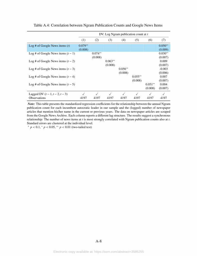
Table A.4: Correlation between Ngram Publication Counts and Google News Items

DV: Log Ngram publication count at t

(1) (2) (3) (4) (5) (6) (7)

Log # of Google News items (t) 0.079∗∗ 0.050∗∗

(0.008) (0.009)Log # of Google News items (t − 1) 0.074∗∗ 0.030∗∗

(0.008) (0.007)Log # of Google News items (t − 2) 0.063∗∗ 0.009

(0.008) (0.007)Log # of Google News items (t − 3) 0.056∗∗ -0.003



(0.008) (0.007)

Lagged DV (t − 1, t − 2, t − 3) X X X X X X XObservations 4197 4197 4197 4197 4197 4197 4197

Note: This table presents the standardized regression coefficients for the relationship between the annual Ngrampublication count for each incumbent autocratic leader in our sample and the (logged) number of newspaperarticles that mention his/her name in the current or previous years. The data on newspaper articles are scrapedfrom the Google News Archive. Each column reports a different lag structure. The results suggest a synchronousrelationship: The number of news items at t is most strongly correlated with Ngram publication counts also at t.Standard errors are clustered at the individual level.+ p < 0.1, ∗ p < 0.05, ∗∗ p < 0.01 (two-tailed test)

A-8


Table A.5: Correlation between Ngram publication counts and New York Times (NYT)Articles (t)

DV: Log Ngram publication count at t

(1) (2) (3) (4) (5) (6) (7)

Log # of NYT articles (t) 0.046∗∗ 0.098∗∗

(0.003) (0.007)Log # of NYT articles (t − 1) 0.031∗∗ -0.009

(0.003) (0.005)Log # of NYT articles (t − 2) 0.025∗∗ -0.023∗

(0.002) (0.005)Log # of NYT articles (t − 3) 0.023∗∗ -0.025∗∗



(0.002) (0.004)

Lagged DV (t − 1, t − 2, t − 3) X X X X X X XObservations 3206 3204 3202 3200 3198 3196 3196

Note: This table presents the standardized regression coefficients for the relationship between the annualNgram publication count for each incumbent autocratic leader in our sample and the (logged) number ofNew York Times articles that mention his/her name in the current or previous years. The data on NYTarticles are accessed through the NYT Article Search API. Each column reports a different lag structure.The results suggest a synchronous relationship: The number of NYT articles at t is most strongly correlatedwith Ngram publication counts also at t. Standard errors are clustered at the individual level.+ p < 0.1, ∗ p < 0.05, ∗∗ p < 0.01 (two-tailed test)

B.2 Construction Procedures

Constructing the Politician List

We constructed the global politician database using information from Wikidata, an open knowledgebase hosted by Wikimedia Foundation. Wikidata is a structured database that allows researchers toretrieve the basic information about individuals recorded in Wikipedia entries, including their birthyear, death year, key occupations, country affiliations, and so on. We created the list of politiciansby identifying individuals whose Occupation Property (P106) included Politician (Q82955).32 Foreach of the politicians we identified, we also collected information on their birth and death years(P569 and P570) and country affiliation (P27).

Once we had a list of politicians, we could further refine it. The basic biographical informationprovided by Wikidata enabled us to identify those who were working concurrently with the nationalchief executive in each country–year. Here, a “concurrent” politician is a living figure who is overthe age of 20 and working in the same country as the chief executive in that year. Since the Ngramcorpus may have different coverages for different countries in different years, a naive approach

32Wikidata provides a structured form to organize information based on two basic concepts: Item and Property.Item represents topics, concepts, or objects, while property represents the connection type between two items. In ourcase, we first find all items whose property instance (P31) is Human (Q5). We then take the items whose Occupationproperty (P106) includes Politician (Q82955). For more details, see the concept section at https://en.wikipedia.org/wiki/Wikidata

A-9


https://en.wikipedia.org/wiki/Wikidata

https://en.wikipedia.org/wiki/Wikidata

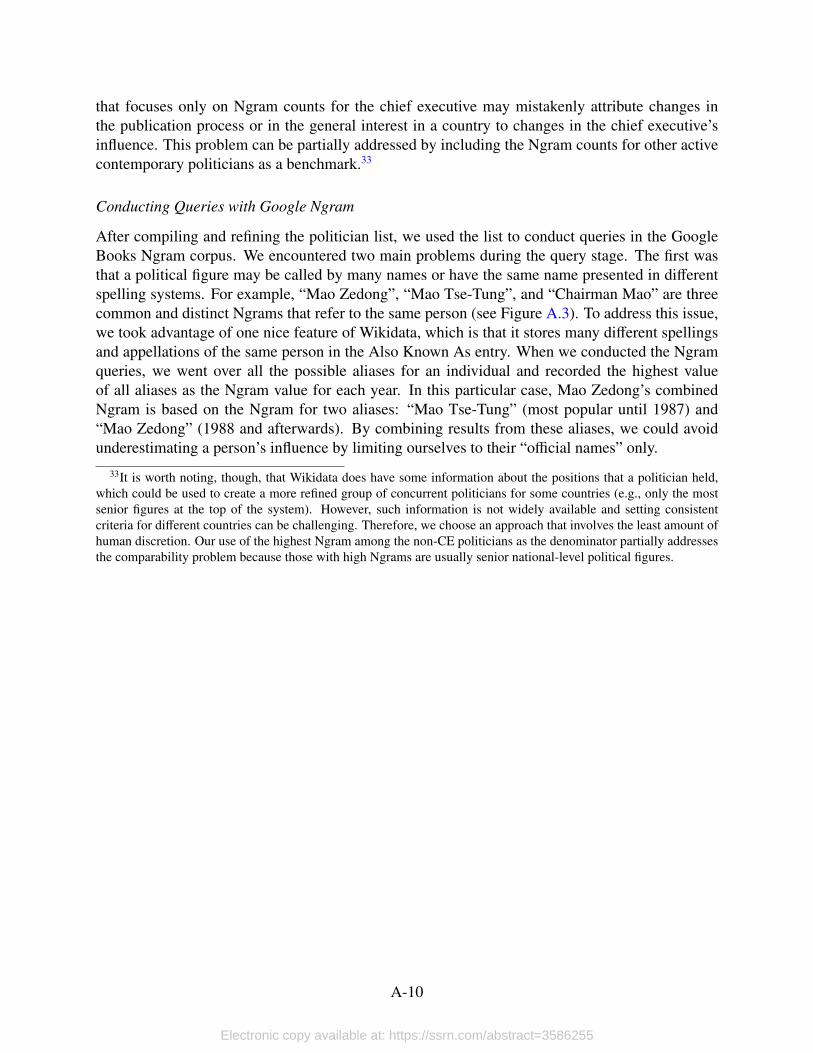
that focuses only on Ngram counts for the chief executive may mistakenly attribute changes inthe publication process or in the general interest in a country to changes in the chief executive’sinfluence. This problem can be partially addressed by including the Ngram counts for other activecontemporary politicians as a benchmark.33

Conducting Queries with Google Ngram

After compiling and refining the politician list, we used the list to conduct queries in the GoogleBooks Ngram corpus. We encountered two main problems during the query stage. The first wasthat a political figure may be called by many names or have the same name presented in differentspelling systems. For example, “Mao Zedong”, “Mao Tse-Tung”, and “Chairman Mao” are threecommon and distinct Ngrams that refer to the same person (see Figure A.3). To address this issue,we took advantage of one nice feature of Wikidata, which is that it stores many different spellingsand appellations of the same person in the Also Known As entry. When we conducted the Ngramqueries, we went over all the possible aliases for an individual and recorded the highest valueof all aliases as the Ngram value for each year. In this particular case, Mao Zedong’s combinedNgram is based on the Ngram for two aliases: “Mao Tse-Tung” (most popular until 1987) and“Mao Zedong” (1988 and afterwards). By combining results from these aliases, we could avoidunderestimating a person’s influence by limiting ourselves to their “official names” only.

33It is worth noting, though, that Wikidata does have some information about the positions that a politician held,which could be used to create a more refined group of concurrent politicians for some countries (e.g., only the mostsenior figures at the top of the system). However, such information is not widely available and setting consistentcriteria for different countries can be challenging. Therefore, we choose an approach that involves the least amount ofhuman discretion. Our use of the highest Ngram among the non-CE politicians as the denominator partially addressesthe comparability problem because those with high Ngrams are usually senior national-level political figures.

A-10


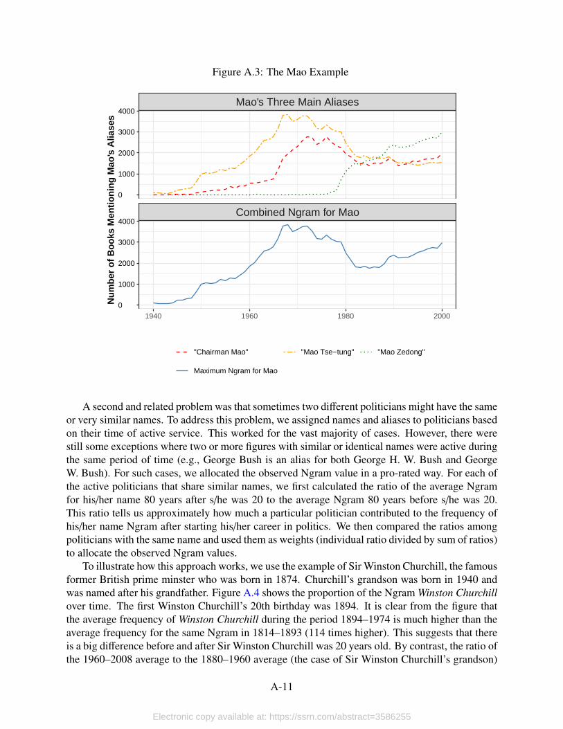
Figure A.3: The Mao Example

Combined Ngram for Mao

Mao's Three Main Aliases

1940 1960 1980 2000

0

1000

2000

3000

4000

0

1000

2000

3000

4000

Num

ber

of B

ooks

Men

tioni

ng M

ao's

Alia

ses

"Chairman Mao" "Mao Tse−tung" "Mao Zedong"

Maximum Ngram for Mao

A second and related problem was that sometimes two different politicians might have the sameor very similar names. To address this problem, we assigned names and aliases to politicians basedon their time of active service. This worked for the vast majority of cases. However, there werestill some exceptions where two or more figures with similar or identical names were active duringthe same period of time (e.g., George Bush is an alias for both George H. W. Bush and GeorgeW. Bush). For such cases, we allocated the observed Ngram value in a pro-rated way. For each ofthe active politicians that share similar names, we first calculated the ratio of the average Ngramfor his/her name 80 years after s/he was 20 to the average Ngram 80 years before s/he was 20.This ratio tells us approximately how much a particular politician contributed to the frequency ofhis/her name Ngram after starting his/her career in politics. We then compared the ratios amongpoliticians with the same name and used them as weights (individual ratio divided by sum of ratios)to allocate the observed Ngram values.

To illustrate how this approach works, we use the example of Sir Winston Churchill, the famousformer British prime minster who was born in 1874. Churchill’s grandson was born in 1940 andwas named after his grandfather. Figure A.4 shows the proportion of the Ngram Winston Churchillover time. The first Winston Churchill’s 20th birthday was 1894. It is clear from the figure thatthe average frequency of Winston Churchill during the period 1894–1974 is much higher than theaverage frequency for the same Ngram in 1814–1893 (114 times higher). This suggests that thereis a big difference before and after Sir Winston Churchill was 20 years old. By contrast, the ratio ofthe 1960–2008 average to the 1880–1960 average (the case of Sir Winston Churchill’s grandson)

A-11


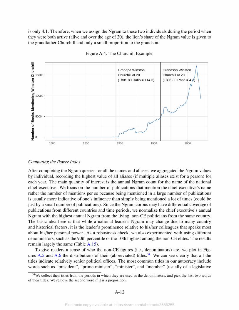
is only 4.1. Therefore, when we assign the Ngram to these two individuals during the period whenthey were both active (alive and over the age of 20), the lion’s share of the Ngram value is given tothe grandfather Churchill and only a small proportion to the grandson.

Figure A.4: The Churchill Example

Grandpa WinstonChurchill at 20

(+80/−80 Ratio = 114.3)

Grandson WinstonChurchill at 20

(+80/−80 Ratio = 4.1)

0

5000

10000

15000

1800 1850 1900 1950 2000

Num

ber

of B

ooks

Men

tioni

ng W

inst

on C

hurc

hill

Computing the Power Index

After completing the Ngram queries for all the names and aliases, we aggregated the Ngram valuesby individual, recording the highest value of all aliases (if multiple aliases exist for a person) foreach year. The main quantity of interest is the annual Ngram count for the name of the nationalchief executive. We focus on the number of publications that mention the chief executive’s namerather the number of mentions per se because being mentioned in a large number of publicationsis usually more indicative of one’s influence than simply being mentioned a lot of times (could bejust by a small number of publications). Since the Ngram corpus may have differential coverage ofpublications from different countries and time periods, we normalize the chief executive’s annualNgram with the highest annual Ngram from the living, non-CE politicians from the same country.The basic idea here is that while a national leader’s Ngram may change due to many countryand historical factors, it is the leader’s prominence relative to his/her colleagues that speaks mostabout his/her personal power. As a robustness check, we also experimented with using differentdenominators, such as the 90th percentile or the 10th highest among the non-CE elites. The resultsremain largely the same (Table A.15).

To give readers a sense of who the non-CE figures (i.e., denominators) are, we plot in Fig-ures A.5 and A.6 the distributions of their (abbreviated) titles.34 We can see clearly that all thetitles indicate relatively senior political offices. The most common titles in our autocracy includewords such as “president”, “prime minister”, “minister”, and “member” (usually of a legislative

34We collect their titles from the periods in which they are used as the denominators, and pick the first two wordsof their titles. We remove the second word if it is a preposition.

A-12


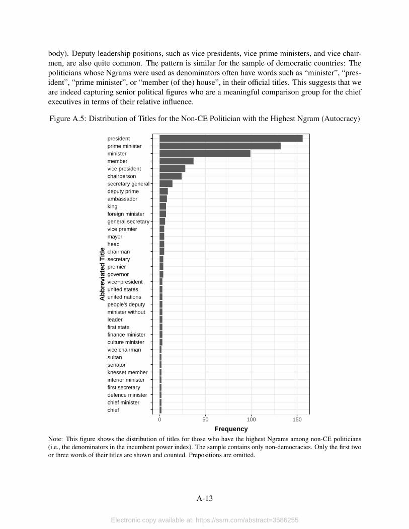
body). Deputy leadership positions, such as vice presidents, vice prime ministers, and vice chair-men, are also quite common. The pattern is similar for the sample of democratic countries: Thepoliticians whose Ngrams were used as denominators often have words such as “minister”, “pres-ident”, “prime minister”, or “member (of the) house”, in their official titles. This suggests that weare indeed capturing senior political figures who are a meaningful comparison group for the chiefexecutives in terms of their relative influence.

Figure A.5: Distribution of Titles for the Non-CE Politician with the Highest Ngram (Autocracy)

chiefchief ministerdefence ministerfirst secretaryinterior ministerknesset membersenatorsultanvice chairmanculture ministerfinance ministerfirst stateleaderminister withoutpeople's deputyunited nationsunited statesvice−presidentgovernorpremiersecretarychairmanheadmayorvice premiergeneral secretaryforeign ministerkingambassadordeputy primesecretary generalchairpersonvice presidentmemberministerprime ministerpresident

0 50 100 150

Frequency

Abb

revi

ated

Titl

e

Note: This figure shows the distribution of titles for those who have the highest Ngrams among non-CE politicians(i.e., the denominators in the incumbent power index). The sample contains only non-democracies. Only the first twoor three words of their titles are shown and counted. Prepositions are omitted.

A-13


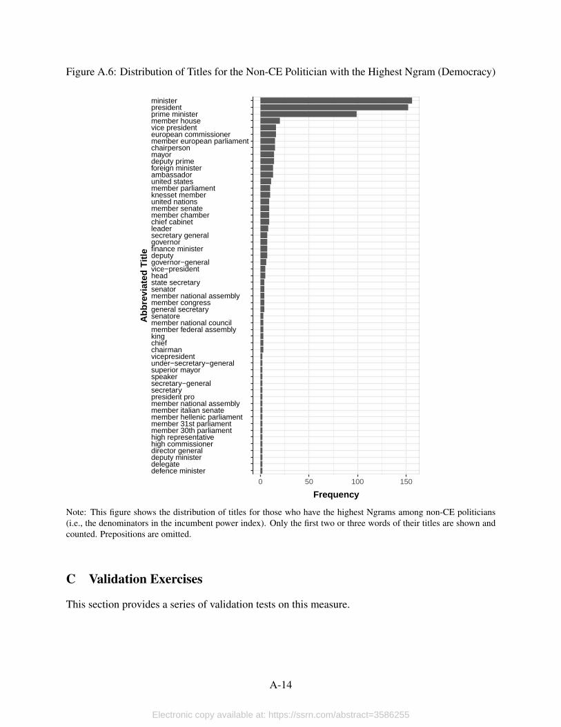
Figure A.6: Distribution of Titles for the Non-CE Politician with the Highest Ngram (Democracy)

defence ministerdelegatedeputy ministerdirector generalhigh commissionerhigh representativemember 30th parliamentmember 31st parliamentmember hellenic parliamentmember italian senatemember national assembly president prosecretarysecretary−generalspeakersuperior mayorunder−secretary−generalvicepresidentchairmanchiefkingmember federal assemblymember national councilsenatoregeneral secretarymember congress member national assemblysenatorstate secretaryheadvice−presidentgovernor−generaldeputyfinance ministergovernorsecretary generalleaderchief cabinetmember chamber member senate united nationsknesset membermember parliament united statesambassadorforeign ministerdeputy primemayorchairpersonmember european parliamenteuropean commissionervice presidentmember house prime ministerpresidentminister

0 50 100 150

Frequency

Abb

revi

ated

Titl

e

Note: This figure shows the distribution of titles for those who have the highest Ngrams among non-CE politicians(i.e., the denominators in the incumbent power index). Only the first two or three words of their titles are shown andcounted. Prepositions are omitted.

C Validation Exercises

This section provides a series of validation tests on this measure.

A-14


C.1 Examples

To get a more substantive sense of how our Ngram measure tracks the rise and fall of autocraticleaders’ power, we provide three validating examples. In each example, our measure is examinedalongside the GWF personalism index and the GS power consolidation measure.

The first case we examine is Tanzania, a country ruled by the Tanganyika African NationalUnion (TANU) party (later Chama Cha Mapinduzi party) since 1964. Tanzania was originallylabeled a single-party regime, but it has held semi-competitive multi-party elections since 1992.Five individuals have served as the chief political executive (President of Tanzania) during thisperiod: Julius Nyerere, Ali Hassan Mwinyi, Benjamin Mkapa, Jakaya Kikwete, and John Magufuli(only available in Ngram). In a way, Tanzania represents a relatively easy case because there isquite a clear difference between the leaders in terms of personal power. As the founding fatherof both the country and the ruling party, Nyerere was clearly the most influential figure of all. Hewas the longest serving president in the history of Tanzania and remained highly active after he leftoffice in 1985. He was an open critic of the economic policies of his successor, Ali Hassan Mwinyi,and was also instrumental in ensuring that Benjamin Mkapa was chosen to succeed Mwinyi in1995. As can be seen in Figure A.7, all three measures broadly agree on the gradations of power:Nyerere clearly overshadows all his successors by a sizable margin, and the personal power ofthe subsequent leaders becomes progressively smaller as Tanzania moves from one-party rule to amulti-party system.

A-15


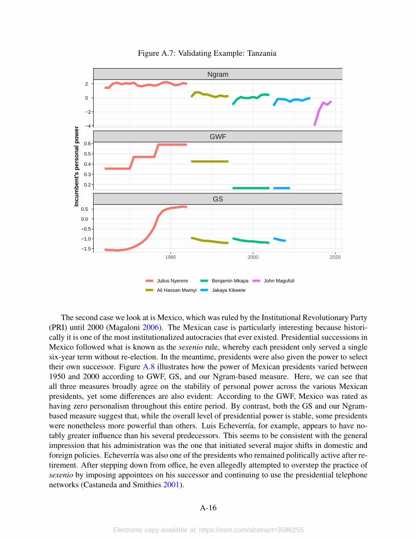
Figure A.7: Validating Example: Tanzania

GS

GWF

Ngram

1980 2000 2020

−4

−2

0

2

0.2

0.3

0.4

0.5

0.6

−1.5

−1.0

−0.5

0.0

0.5

Incu

mbe

nt's

per

sona

l pow

er

Julius Nyerere

Ali Hassan Mwinyi

Benjamin Mkapa

Jakaya Kikwete

John Magufuli

The second case we look at is Mexico, which was ruled by the Institutional Revolutionary Party(PRI) until 2000 (Magaloni 2006). The Mexican case is particularly interesting because histori-cally it is one of the most institutionalized autocracies that ever existed. Presidential successions inMexico followed what is known as the sexenio rule, whereby each president only served a singlesix-year term without re-election. In the meantime, presidents were also given the power to selecttheir own successor. Figure A.8 illustrates how the power of Mexican presidents varied between1950 and 2000 according to GWF, GS, and our Ngram-based measure. Here, we can see thatall three measures broadly agree on the stability of personal power across the various Mexicanpresidents, yet some differences are also evident: According to the GWF, Mexico was rated ashaving zero personalism throughout this entire period. By contrast, both the GS and our Ngram-based measure suggest that, while the overall level of presidential power is stable, some presidentswere nonetheless more powerful than others. Luis Echeverrıa, for example, appears to have no-tably greater influence than his several predecessors. This seems to be consistent with the generalimpression that his administration was the one that initiated several major shifts in domestic andforeign policies. Echeverrıa was also one of the presidents who remained politically active after re-tirement. After stepping down from office, he even allegedly attempted to overstep the practice ofsexenio by imposing appointees on his successor and continuing to use the presidential telephonenetworks (Castaneda and Smithies 2001).

A-16


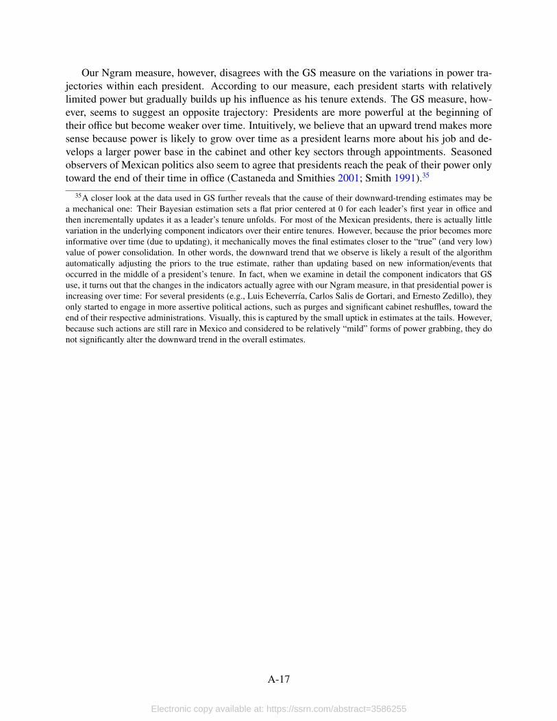
Our Ngram measure, however, disagrees with the GS measure on the variations in power tra-jectories within each president. According to our measure, each president starts with relativelylimited power but gradually builds up his influence as his tenure extends. The GS measure, how-ever, seems to suggest an opposite trajectory: Presidents are more powerful at the beginning oftheir office but become weaker over time. Intuitively, we believe that an upward trend makes moresense because power is likely to grow over time as a president learns more about his job and de-velops a larger power base in the cabinet and other key sectors through appointments. Seasonedobservers of Mexican politics also seem to agree that presidents reach the peak of their power onlytoward the end of their time in office (Castaneda and Smithies 2001; Smith 1991).35

35A closer look at the data used in GS further reveals that the cause of their downward-trending estimates may bea mechanical one: Their Bayesian estimation sets a flat prior centered at 0 for each leader’s first year in office andthen incrementally updates it as a leader’s tenure unfolds. For most of the Mexican presidents, there is actually littlevariation in the underlying component indicators over their entire tenures. However, because the prior becomes moreinformative over time (due to updating), it mechanically moves the final estimates closer to the “true” (and very low)value of power consolidation. In other words, the downward trend that we observe is likely a result of the algorithmautomatically adjusting the priors to the true estimate, rather than updating based on new information/events thatoccurred in the middle of a president’s tenure. In fact, when we examine in detail the component indicators that GSuse, it turns out that the changes in the indicators actually agree with our Ngram measure, in that presidential power isincreasing over time: For several presidents (e.g., Luis Echeverrıa, Carlos Salis de Gortari, and Ernesto Zedillo), theyonly started to engage in more assertive political actions, such as purges and significant cabinet reshuffles, toward theend of their respective administrations. Visually, this is captured by the small uptick in estimates at the tails. However,because such actions are still rare in Mexico and considered to be relatively “mild” forms of power grabbing, they donot significantly alter the downward trend in the overall estimates.

A-17


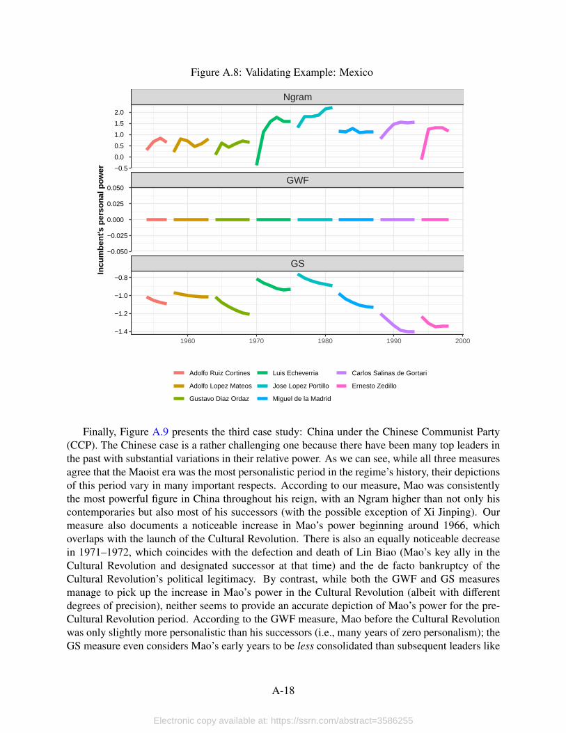
Figure A.8: Validating Example: Mexico

GS

GWF

Ngram

1960 1970 1980 1990 2000

−0.5

0.0

0.5

1.0

1.5

2.0

−0.050

−0.025

0.000

0.025

0.050

−1.4

−1.2

−1.0

−0.8

Incu

mbe

nt's

per

sona

l pow

er

Adolfo Ruiz Cortines

Adolfo Lopez Mateos

Gustavo Diaz Ordaz

Luis Echeverria

Jose Lopez Portillo

Miguel de la Madrid

Carlos Salinas de Gortari

Ernesto Zedillo

Finally, Figure A.9 presents the third case study: China under the Chinese Communist Party(CCP). The Chinese case is a rather challenging one because there have been many top leaders inthe past with substantial variations in their relative power. As we can see, while all three measuresagree that the Maoist era was the most personalistic period in the regime’s history, their depictionsof this period vary in many important respects. According to our measure, Mao was consistentlythe most powerful figure in China throughout his reign, with an Ngram higher than not only hiscontemporaries but also most of his successors (with the possible exception of Xi Jinping). Ourmeasure also documents a noticeable increase in Mao’s power beginning around 1966, whichoverlaps with the launch of the Cultural Revolution. There is also an equally noticeable decreasein 1971–1972, which coincides with the defection and death of Lin Biao (Mao’s key ally in theCultural Revolution and designated successor at that time) and the de facto bankruptcy of theCultural Revolution’s political legitimacy. By contrast, while both the GWF and GS measuresmanage to pick up the increase in Mao’s power in the Cultural Revolution (albeit with differentdegrees of precision), neither seems to provide an accurate depiction of Mao’s power for the pre-Cultural Revolution period. According to the GWF measure, Mao before the Cultural Revolutionwas only slightly more personalistic than his successors (i.e., many years of zero personalism); theGS measure even considers Mao’s early years to be less consolidated than subsequent leaders like

A-18


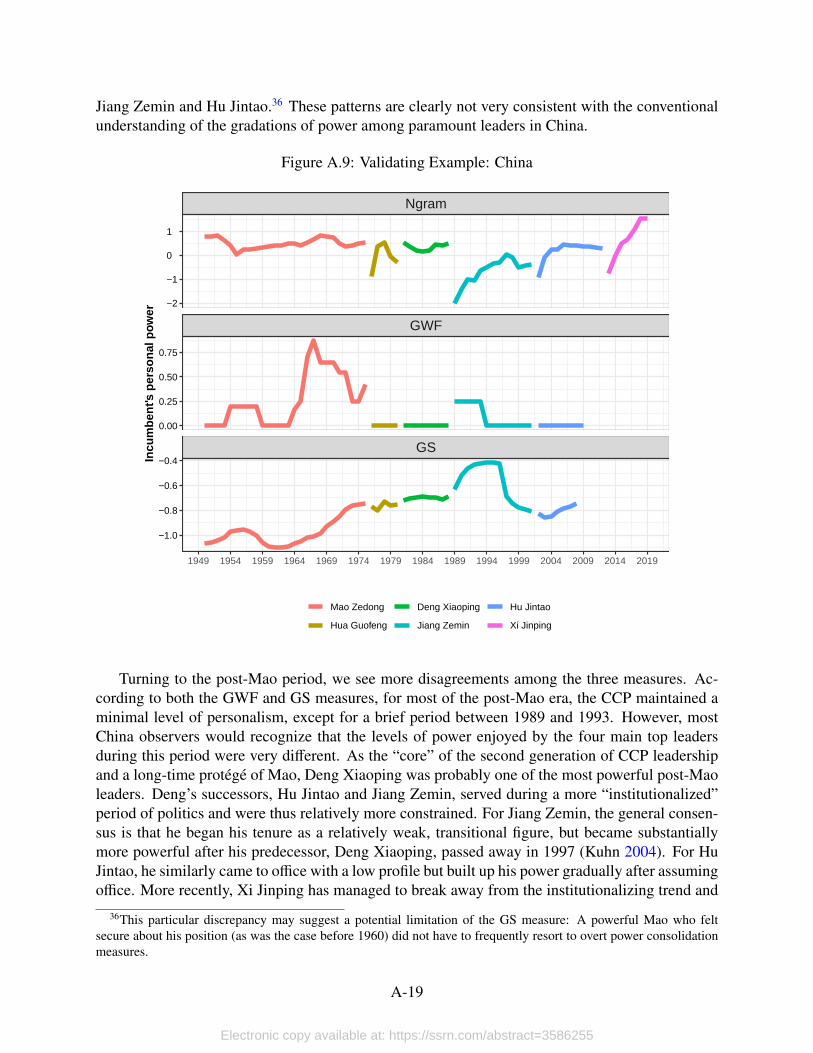
Jiang Zemin and Hu Jintao.36 These patterns are clearly not very consistent with the conventionalunderstanding of the gradations of power among paramount leaders in China.

Figure A.9: Validating Example: China

GS

GWF

Ngram

1949 1954 1959 1964 1969 1974 1979 1984 1989 1994 1999 2004 2009 2014 2019

−2

−1

0

1

0.00

0.25

0.50

0.75

−1.0

−0.8

−0.6

−0.4Incu

mbe

nt's

per

sona

l pow

er

Mao Zedong

Hua Guofeng

Deng Xiaoping

Jiang Zemin

Hu Jintao

Xi Jinping

Turning to the post-Mao period, we see more disagreements among the three measures. Ac-cording to both the GWF and GS measures, for most of the post-Mao era, the CCP maintained aminimal level of personalism, except for a brief period between 1989 and 1993. However, mostChina observers would recognize that the levels of power enjoyed by the four main top leadersduring this period were very different. As the “core” of the second generation of CCP leadershipand a long-time protege of Mao, Deng Xiaoping was probably one of the most powerful post-Maoleaders. Deng’s successors, Hu Jintao and Jiang Zemin, served during a more “institutionalized”period of politics and were thus relatively more constrained. For Jiang Zemin, the general consen-sus is that he began his tenure as a relatively weak, transitional figure, but became substantiallymore powerful after his predecessor, Deng Xiaoping, passed away in 1997 (Kuhn 2004). For HuJintao, he similarly came to office with a low profile but built up his power gradually after assumingoffice. More recently, Xi Jinping has managed to break away from the institutionalizing trend and

36This particular discrepancy may suggest a potential limitation of the GS measure: A powerful Mao who feltsecure about his position (as was the case before 1960) did not have to frequently resort to overt power consolidationmeasures.

A-19


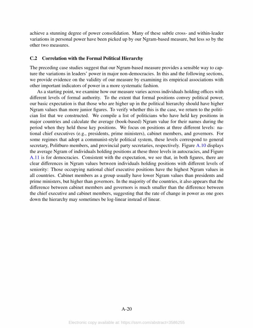
achieve a stunning degree of power consolidation. Many of these subtle cross- and within-leadervariations in personal power have been picked up by our Ngram-based measure, but less so by theother two measures.

C.2 Correlation with the Formal Political Hierarchy

The preceding case studies suggest that our Ngram-based measure provides a sensible way to cap-ture the variations in leaders’ power in major non-democracies. In this and the following sections,we provide evidence on the validity of our measure by examining its empirical associations withother important indicators of power in a more systematic fashion.

As a starting point, we examine how our measure varies across individuals holding offices withdifferent levels of formal authority. To the extent that formal positions convey political power,our basic expectation is that those who are higher up in the political hierarchy should have higherNgram values than more junior figures. To verify whether this is the case, we return to the politi-cian list that we constructed. We compile a list of politicians who have held key positions inmajor countries and calculate the average (book-based) Ngram value for their names during theperiod when they held those key positions. We focus on positions at three different levels: na-tional chief executives (e.g., presidents, prime ministers), cabinet members, and governors. Forsome regimes that adopt a communist-style political system, these levels correspond to generalsecretary, Politburo members, and provincial party secretaries, respectively. Figure A.10 displaysthe average Ngram of individuals holding positions at these three levels in autocracies, and FigureA.11 is for democracies. Consistent with the expectation, we see that, in both figures, there areclear differences in Ngram values between individuals holding positions with different levels ofseniority: Those occupying national chief executive positions have the highest Ngram values inall countries. Cabinet members as a group usually have lower Ngram values than presidents andprime ministers, but higher than governors. In the majority of the countries, it also appears that thedifference between cabinet members and governors is much smaller than the difference betweenthe chief executive and cabinet members, suggesting that the rate of change in power as one goesdown the hierarchy may sometimes be log-linear instead of linear.

A-20


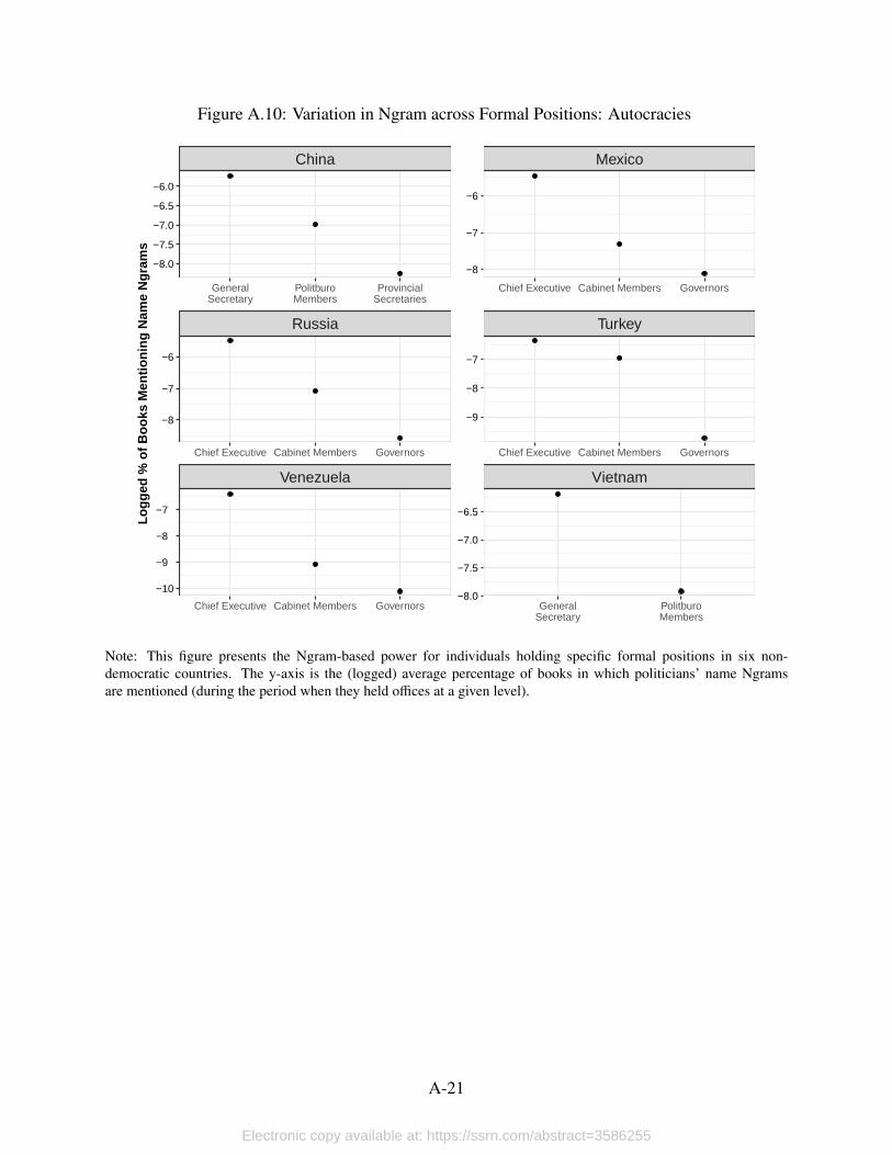
Figure A.10: Variation in Ngram across Formal Positions: Autocracies

Venezuela Vietnam

Russia Turkey

China Mexico

Chief Executive Cabinet Members Governors GeneralSecretary

PolitburoMembers

Chief Executive Cabinet Members Governors Chief Executive Cabinet Members Governors

GeneralSecretary

PolitburoMembers

ProvincialSecretaries

Chief Executive Cabinet Members Governors

−8

−7

−6

−9

−8

−7

−8.0

−7.5

−7.0

−6.5

−8.0

−7.5

−7.0

−6.5

−6.0

−8

−7

−6

−10

−9

−8

−7

Logg

ed %

of B

ooks

Men

tioni

ng N

ame

Ngr

ams

Note: This figure presents the Ngram-based power for individuals holding specific formal positions in six non-democratic countries. The y-axis is the (logged) average percentage of books in which politicians’ name Ngramsare mentioned (during the period when they held offices at a given level).

A-21


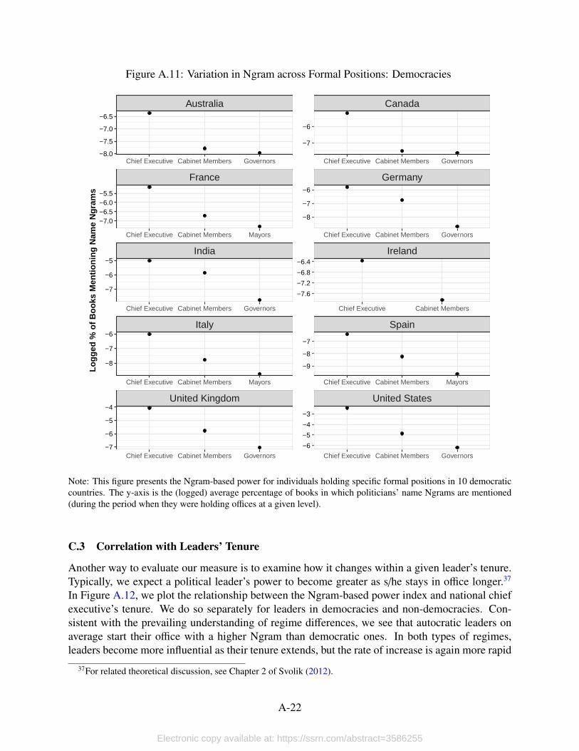
Figure A.11: Variation in Ngram across Formal Positions: Democracies

United Kingdom United States

Italy Spain

India Ireland

France Germany

Australia Canada


Chief Executive Cabinet Members Mayors Chief Executive Cabinet Members Mayors

Chief Executive Cabinet Members Governors Chief Executive Cabinet Members

Chief Executive Cabinet Members Mayors Chief Executive Cabinet Members Governors


−7

−6

−8

−7

−6

−7.6

−7.2

−6.8

−6.4

−9

−8

−7

−6

−5

−4

−3

−8.0

−7.5

−7.0

−6.5

−7.0−6.5−6.0−5.5

−7

−6

−5

−8

−7

−6

−7

−6

−5

−4

Logg

ed %

of B

ooks

Men

tioni

ng N

ame

Ngr

ams

Note: This figure presents the Ngram-based power for individuals holding specific formal positions in 10 democraticcountries. The y-axis is the (logged) average percentage of books in which politicians’ name Ngrams are mentioned(during the period when they were holding offices at a given level).

C.3 Correlation with Leaders’ Tenure

Another way to evaluate our measure is to examine how it changes within a given leader’s tenure.Typically, we expect a political leader’s power to become greater as s/he stays in office longer.37

In Figure A.12, we plot the relationship between the Ngram-based power index and national chiefexecutive’s tenure. We do so separately for leaders in democracies and non-democracies. Con-sistent with the prevailing understanding of regime differences, we see that autocratic leaders onaverage start their office with a higher Ngram than democratic ones. In both types of regimes,leaders become more influential as their tenure extends, but the rate of increase is again more rapid

37For related theoretical discussion, see Chapter 2 of Svolik (2012).

A-22


in autocracies than in democracies.

Figure A.12: Variation in Ngram Over Leaders’ Tenure

0

1

less than 5 yrs 5−10 yrs 10−20 yrs 20−30 yrs over 30 yrs

Ngr

am−b

ased

pow

er in

dex

Democracy Autocracy

Note: This figure shows the change in Ngram-based power over leaders’ tenure. We plot the relationship separatelyfor democracies and autocracies. The vertical bars represent the 95% confidence intervals.

C.4 Correlation with Electoral Outcomes

Third, we can also verify our measure by studying how it correlates with electoral outcomes. Tothe extent that elections are essentially a civilized form of power contest (Przeworski 2018), theoutcome of elections should reflect the power parity between contending candidates. Those whohave the ability to marshal a great amount of resources or the loyalty of a large group of individualsare more likely to emerge victorious in the electoral arena. We thus expect that such strength willalso be reflected in candidates’ Ngram values.

To verify whether this is indeed the case, we collect information about the leading candidates38

and outcomes of national-level general elections for all democratic countries between 1950 and2008. We obtain each candidate’s Ngram value one year before the election and examine how thesevalues correlate with candidates’ performance in elections. Figure A.13 shows how the differencebetween the winner’s and (closest) loser’s Ngram values corresponds to the electoral margin ofthe winner. We can see that there is a clear, positive relationship. The winner’s margin over theclosest loser becomes progressively greater as his/her Ngram value gets larger relative to that of theopponent. In Table A.6, we estimate the association between candidates’ Ngram and their electoralperformance. The first two columns show that the winner’s margin is positively associated withthe winner’s own Ngram value one year before the election and negatively associated with that ofthe closest loser. This pattern holds even when we limit the sample to open-seat elections in whichno incumbent is running. Columns 3 and 4 further examine the vote shares for the winner and the

38For simplicity, we only focus on the two candidates who won the first and second highest vote share.

A-23


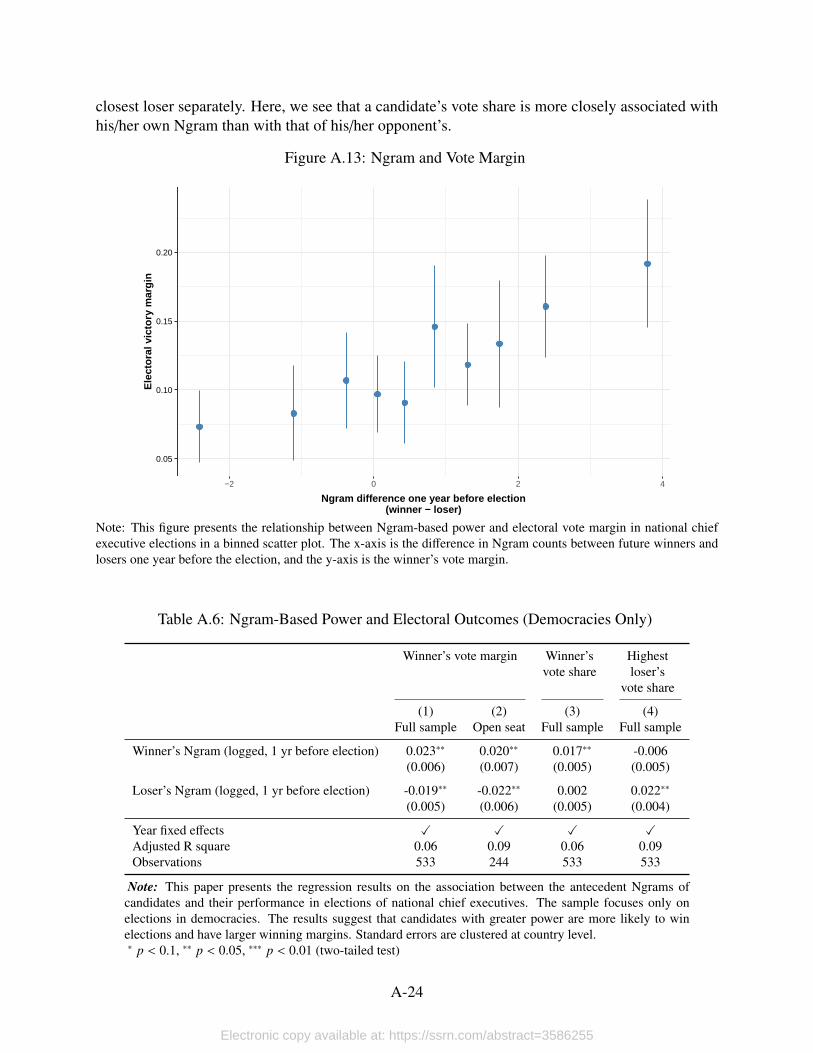
closest loser separately. Here, we see that a candidate’s vote share is more closely associated withhis/her own Ngram than with that of his/her opponent’s.

Figure A.13: Ngram and Vote Margin

0.05

0.10

0.15

0.20

−2 0 2 4

Ngram difference one year before election(winner − loser)

Ele

ctor

al v

icto

ry m

argi

n

Note: This figure presents the relationship between Ngram-based power and electoral vote margin in national chiefexecutive elections in a binned scatter plot. The x-axis is the difference in Ngram counts between future winners andlosers one year before the election, and the y-axis is the winner’s vote margin.

Table A.6: Ngram-Based Power and Electoral Outcomes (Democracies Only)

Winner’s vote margin Winner’svote share

Highestloser’s

vote share

(1) (2) (3) (4)Full sample Open seat Full sample Full sample

Winner’s Ngram (logged, 1 yr before election) 0.023∗∗ 0.020∗∗ 0.017∗∗ -0.006(0.006) (0.007) (0.005) (0.005)

Loser’s Ngram (logged, 1 yr before election) -0.019∗∗ -0.022∗∗ 0.002 0.022∗∗

(0.005) (0.006) (0.005) (0.004)

Year fixed effects X X X XAdjusted R square 0.06 0.09 0.06 0.09Observations 533 244 533 533

Note: This paper presents the regression results on the association between the antecedent Ngrams ofcandidates and their performance in elections of national chief executives. The sample focuses only onelections in democracies. The results suggest that candidates with greater power are more likely to winelections and have larger winning margins. Standard errors are clustered at country level.∗ p < 0.1, ∗∗ p < 0.05, ∗∗∗ p < 0.01 (two-tailed test)

A-24


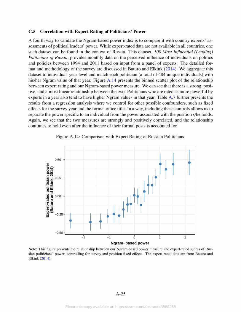
C.5 Correlation with Expert Rating of Politicians’ Power

A fourth way to validate the Ngram-based power index is to compare it with country experts’ as-sessments of political leaders’ power. While expert-rated data are not available in all countries, onesuch dataset can be found in the context of Russia. This dataset, 100 Most Influential (Leading)Politicians of Russia, provides monthly data on the perceived influence of individuals on politicsand policies between 1994 and 2011 based on input from a panel of experts. The detailed for-mat and methodology of the survey are discussed in Baturo and Elkink (2014). We aggregate thisdataset to individual–year level and match each politician (a total of 484 unique individuals) withhis/her Ngram value of that year. Figure A.14 presents the binned scatter plot of the relationshipbetween expert rating and our Ngram-based power measure. We can see that there is a strong, posi-tive, and almost linear relationship between the two. Politicians who are rated as more powerful byexperts in a year also tend to have higher Ngram values in that year. Table A.7 further presents theresults from a regression analysis where we control for other possible confounders, such as fixedeffects for the survey year and the formal office title. In a way, including these controls allows us toseparate the power specific to an individual from the power associated with the position s/he holds.Again, we see that the two measures are strongly and positively correlated, and the relationshipcontinues to hold even after the influence of their formal posts is accounted for.

Figure A.14: Comparison with Expert Rating of Russian Politicians

−0.50

−0.25

0.00

0.25

0.50

−2 −1 0 1 2

Ngram−based power

Exp

ert−

rate

d po

litic

ian

pow

er (

Bat

uro

and

Elk

ink,

201

4)

Note: This figure presents the relationship between our Ngram-based power measure and expert-rated scores of Rus-sian politicians’ power, controlling for survey and position fixed effects. The expert-rated data are from Baturo andElkink (2014).

A-25


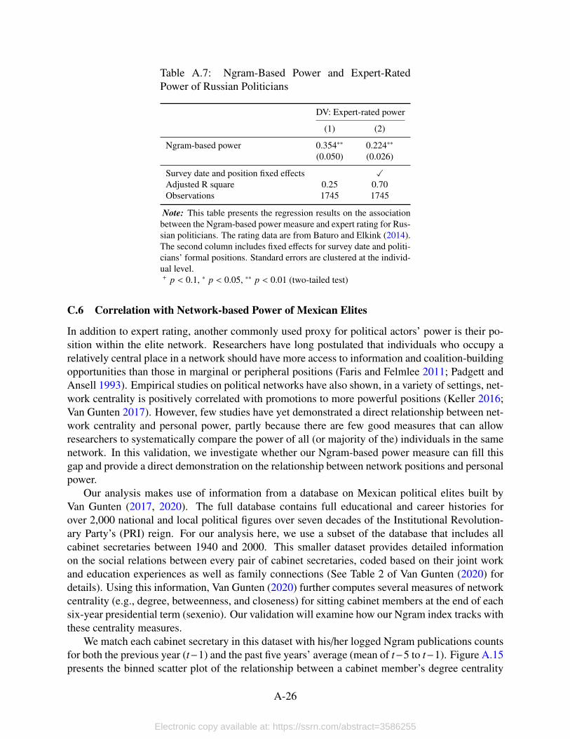
Table A.7: Ngram-Based Power and Expert-RatedPower of Russian Politicians

DV: Expert-rated power

(1) (2)

Ngram-based power 0.354∗∗ 0.224∗∗

(0.050) (0.026)

Survey date and position fixed effects XAdjusted R square 0.25 0.70Observations 1745 1745

Note: This table presents the regression results on the associationbetween the Ngram-based power measure and expert rating for Rus-sian politicians. The rating data are from Baturo and Elkink (2014).The second column includes fixed effects for survey date and politi-cians’ formal positions. Standard errors are clustered at the individ-ual level.+ p < 0.1, ∗ p < 0.05, ∗∗ p < 0.01 (two-tailed test)

C.6 Correlation with Network-based Power of Mexican Elites

In addition to expert rating, another commonly used proxy for political actors’ power is their po-sition within the elite network. Researchers have long postulated that individuals who occupy arelatively central place in a network should have more access to information and coalition-buildingopportunities than those in marginal or peripheral positions (Faris and Felmlee 2011; Padgett andAnsell 1993). Empirical studies on political networks have also shown, in a variety of settings, net-work centrality is positively correlated with promotions to more powerful positions (Keller 2016;Van Gunten 2017). However, few studies have yet demonstrated a direct relationship between net-work centrality and personal power, partly because there are few good measures that can allowresearchers to systematically compare the power of all (or majority of the) individuals in the samenetwork. In this validation, we investigate whether our Ngram-based power measure can fill thisgap and provide a direct demonstration on the relationship between network positions and personalpower.

Our analysis makes use of information from a database on Mexican political elites built byVan Gunten (2017, 2020). The full database contains full educational and career histories forover 2,000 national and local political figures over seven decades of the Institutional Revolution-ary Party’s (PRI) reign. For our analysis here, we use a subset of the database that includes allcabinet secretaries between 1940 and 2000. This smaller dataset provides detailed informationon the social relations between every pair of cabinet secretaries, coded based on their joint workand education experiences as well as family connections (See Table 2 of Van Gunten (2020) fordetails). Using this information, Van Gunten (2020) further computes several measures of networkcentrality (e.g., degree, betweenness, and closeness) for sitting cabinet members at the end of eachsix-year presidential term (sexenio). Our validation will examine how our Ngram index tracks withthese centrality measures.

We match each cabinet secretary in this dataset with his/her logged Ngram publications countsfor both the previous year (t−1) and the past five years’ average (mean of t−5 to t−1). Figure A.15presents the binned scatter plot of the relationship between a cabinet member’s degree centrality

A-26


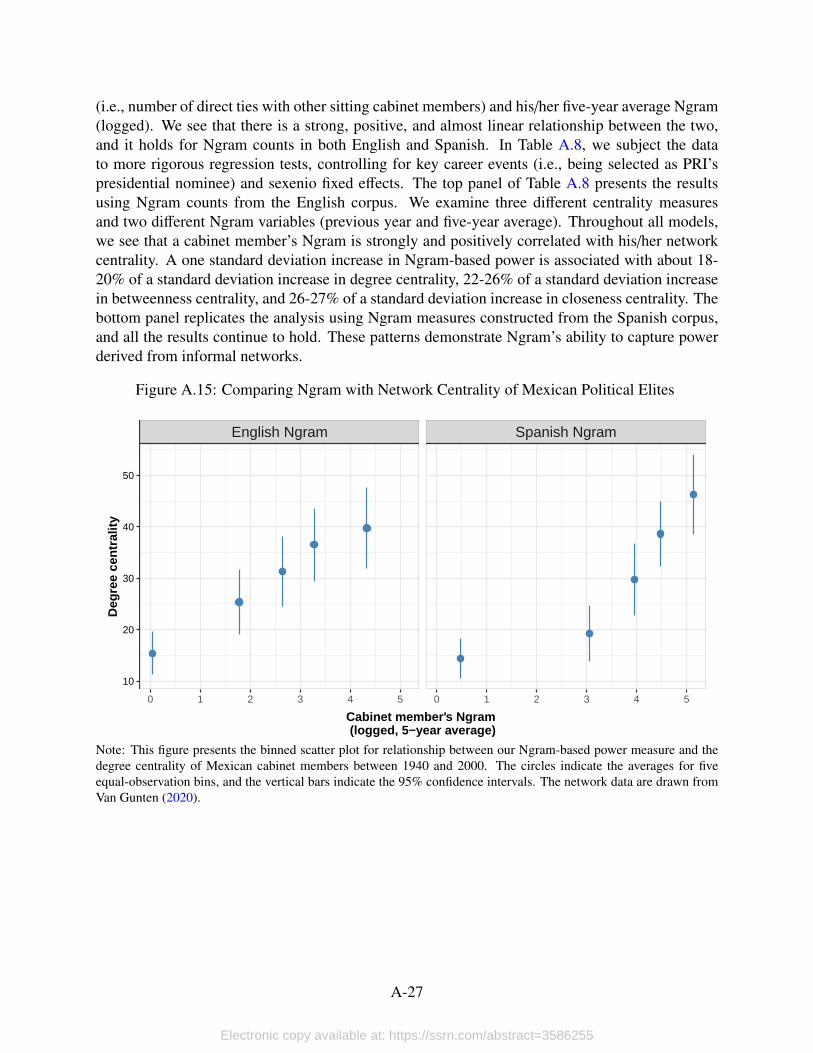
(i.e., number of direct ties with other sitting cabinet members) and his/her five-year average Ngram(logged). We see that there is a strong, positive, and almost linear relationship between the two,and it holds for Ngram counts in both English and Spanish. In Table A.8, we subject the datato more rigorous regression tests, controlling for key career events (i.e., being selected as PRI’spresidential nominee) and sexenio fixed effects. The top panel of Table A.8 presents the resultsusing Ngram counts from the English corpus. We examine three different centrality measuresand two different Ngram variables (previous year and five-year average). Throughout all models,we see that a cabinet member’s Ngram is strongly and positively correlated with his/her networkcentrality. A one standard deviation increase in Ngram-based power is associated with about 18-20% of a standard deviation increase in degree centrality, 22-26% of a standard deviation increasein betweenness centrality, and 26-27% of a standard deviation increase in closeness centrality. Thebottom panel replicates the analysis using Ngram measures constructed from the Spanish corpus,and all the results continue to hold. These patterns demonstrate Ngram’s ability to capture powerderived from informal networks.

Figure A.15: Comparing Ngram with Network Centrality of Mexican Political Elites

English Ngram Spanish Ngram

0 1 2 3 4 5 0 1 2 3 4 5

10

20

30

40

50

Cabinet member's Ngram (logged, 5−year average)

Deg

ree

cent

ralit

y

Note: This figure presents the binned scatter plot for relationship between our Ngram-based power measure and thedegree centrality of Mexican cabinet members between 1940 and 2000. The circles indicate the averages for fiveequal-observation bins, and the vertical bars indicate the 95% confidence intervals. The network data are drawn fromVan Gunten (2020).

A-27


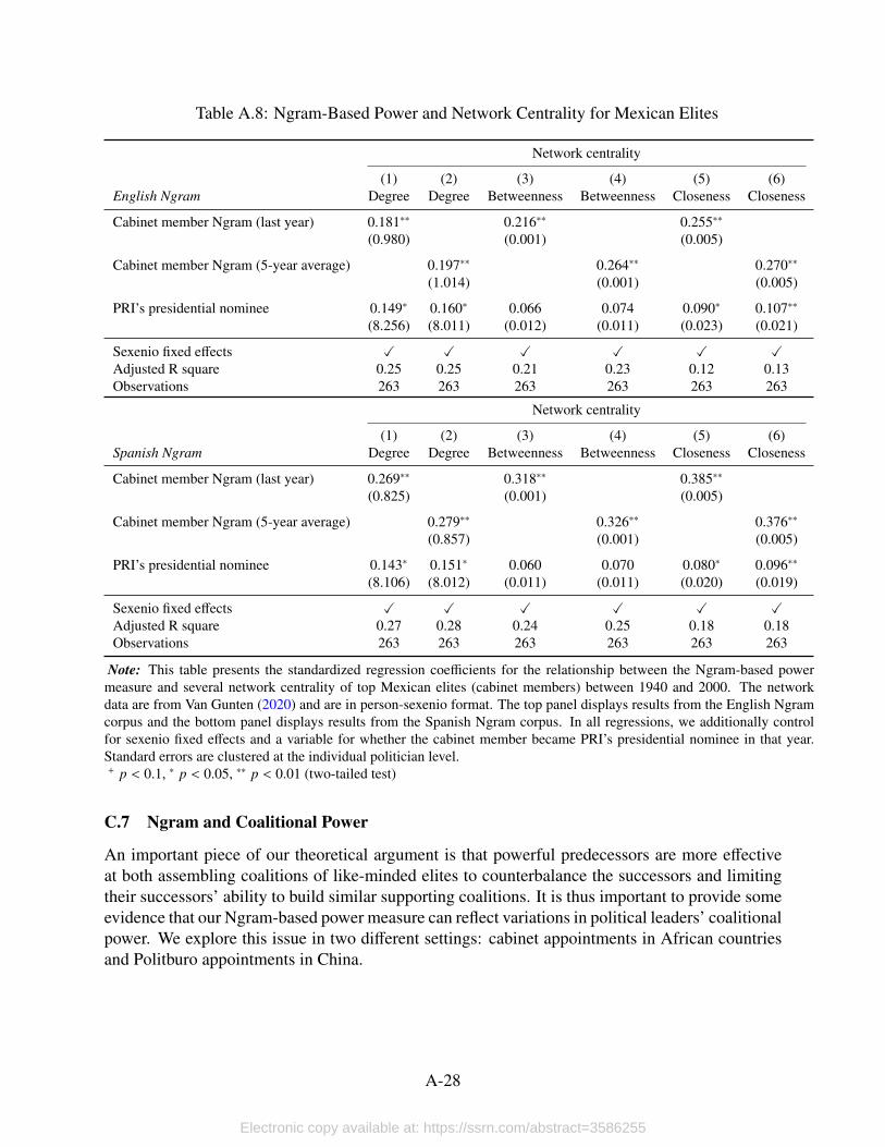
Table A.8: Ngram-Based Power and Network Centrality for Mexican Elites

Network centrality

(1) (2) (3) (4) (5) (6)English Ngram Degree Degree Betweenness Betweenness Closeness Closeness

Cabinet member Ngram (last year) 0.181∗∗ 0.216∗∗ 0.255∗∗

(0.980) (0.001) (0.005)

Cabinet member Ngram (5-year average) 0.197∗∗ 0.264∗∗ 0.270∗∗

(1.014) (0.001) (0.005)

PRI’s presidential nominee 0.149∗ 0.160∗ 0.066 0.074 0.090∗ 0.107∗∗

(8.256) (8.011) (0.012) (0.011) (0.023) (0.021)

Sexenio fixed effects X X X X X XAdjusted R square 0.25 0.25 0.21 0.23 0.12 0.13Observations 263 263 263 263 263 263

Network centrality

(1) (2) (3) (4) (5) (6)Spanish Ngram Degree Degree Betweenness Betweenness Closeness Closeness

Cabinet member Ngram (last year) 0.269∗∗ 0.318∗∗ 0.385∗∗

(0.825) (0.001) (0.005)

Cabinet member Ngram (5-year average) 0.279∗∗ 0.326∗∗ 0.376∗∗

(0.857) (0.001) (0.005)

PRI’s presidential nominee 0.143∗ 0.151∗ 0.060 0.070 0.080∗ 0.096∗∗

(8.106) (8.012) (0.011) (0.011) (0.020) (0.019)

Sexenio fixed effects X X X X X XAdjusted R square 0.27 0.28 0.24 0.25 0.18 0.18Observations 263 263 263 263 263 263

Note: This table presents the standardized regression coefficients for the relationship between the Ngram-based powermeasure and several network centrality of top Mexican elites (cabinet members) between 1940 and 2000. The networkdata are from Van Gunten (2020) and are in person-sexenio format. The top panel displays results from the English Ngramcorpus and the bottom panel displays results from the Spanish Ngram corpus. In all regressions, we additionally controlfor sexenio fixed effects and a variable for whether the cabinet member became PRI’s presidential nominee in that year.Standard errors are clustered at the individual politician level.+ p < 0.1, ∗ p < 0.05, ∗∗ p < 0.01 (two-tailed test)

C.7 Ngram and Coalitional Power

An important piece of our theoretical argument is that powerful predecessors are more effectiveat both assembling coalitions of like-minded elites to counterbalance the successors and limitingtheir successors’ ability to build similar supporting coalitions. It is thus important to provide someevidence that our Ngram-based power measure can reflect variations in political leaders’ coalitionalpower. We explore this issue in two different settings: cabinet appointments in African countriesand Politburo appointments in China.

A-28


C.7.1 Cabinet Appointments in Africa, 1996–2017

We begin by examining how the personal power of African leaders affects their ability to appointtheir co-ethnics to high-level cabinet positions. A prominent feature of politics in many Africancountries is the presence of strong ethnic cleavages. Governments are often founded upon certainconfigurations of ethnic alliances, and the distribution of valuable resources often follows ethniclines (Bates 1981; Bratton and Walle 1997; Francois, Rainer, and Trebbi 2015). It is a commonpractice for top African leaders to recruit their co-ethnics into the elite ruling coalition—usually thecabinet (Arriola 2009; Meng 2020). Making co-ethnic cabinet appointments is both an importantmanifestation of leaders’ power and a common strategy to solidify their position among regimeelites (Arriola 2009; Hassan 2017).

We perform the validation tests by making use of the African Cabinet and Political EliteDatabase (ACPED) developed by Raleigh and Wigmore-Shepherd (2020). The dataset containsinformation on all cabinet ministers who served in 23 African states between 1996 and 2017. Aparticularly useful piece of information that this dataset offers is whether cabinet ministers sharethe same ethnic background as their contemporary national chief executives. We use this informa-tion to compute the percentage of cabinet members who are the sitting national chief executive’sco-ethnics for each country–year spell.39 We then match the dataset with our Ngram database andcalculate, for each national chief executive, his/her Ngram power index for the current year and theaverage index from the past five years. The latter variable is intended to address the reverse causal-ity concern that a large number of co-ethnic appointments may help boost the national leader’ssubsequent power and influence. We estimate the following regression:

Share of incumbent’s co-ethnics in cabinetct = δ Incumbent powerct + Xβ + τt + ηc + εct,

where c and t index country and year, respectively. We include country fixed effects ηc toaccount for the possibility that national leaders from some countries may receive more Ngramcoverage than others, and year fixed effects τt to account for time-variant shocks that affect allstates in the sample. The vector of control covariates include log GDP per capita, log population,and a binary variable for whether a country is a democracy.

Table A.9 displays the regression results. The first column presents the most parsimoniousmodel, in which we only control for country and year fixed effects. Column 2 further includesthe institutional and economic covariates. In Column 3, we address the potential reverse causalityconcern by using the average Ngram for the past five years as the measure of the incumbent’spower. Throughout these models, we find that the Ngram-based measure of incumbent leaders’power is positively associated with the number of co-ethnic appointees in a cabinet. Accordingto the coefficient estimates from Column 2, a one standard deviation increase in an incumbent’spower is associated with about a 3 percentage point increase in co-ethnic cabinet share, whichamounts to about a 12% change from the sample average (29%). This pattern is consistent with thegeneral impression: More powerful African leaders are more capable of building large co-ethnic

39The original dataset is recorded at monthly level. However, since many months do not record any cabinet per-sonnel changes, using a monthly dataset may artificially inflate the number of observations and lead to overstatedstatistical significance. To be conservative, we reduce the original data to an annual dataset by only keeping observa-tions recorded in December of each year.

A-29


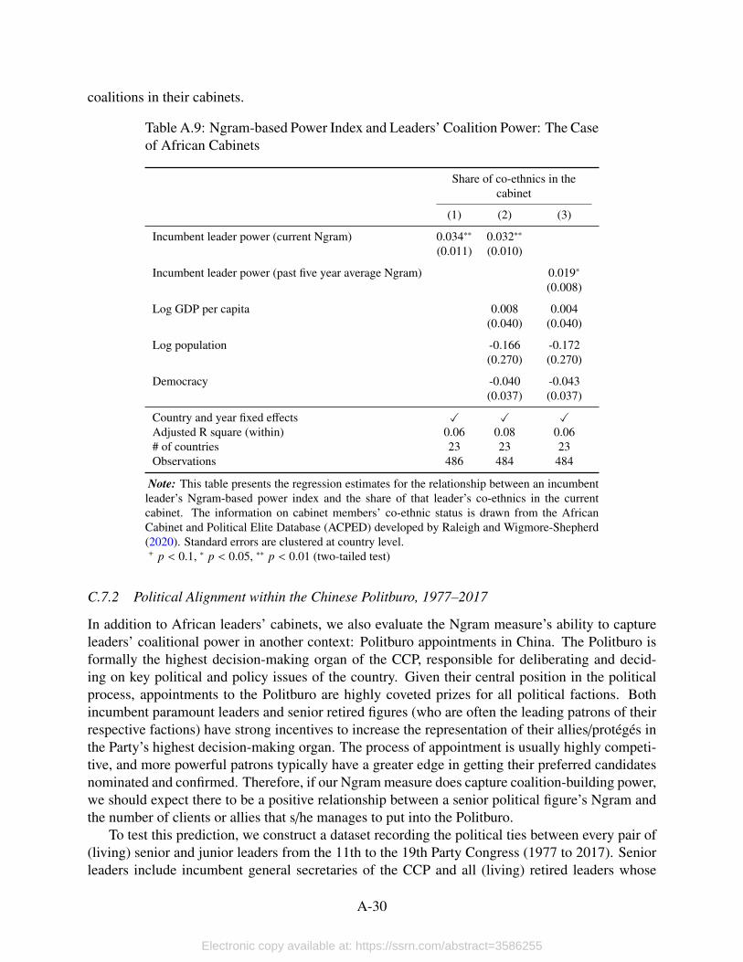
coalitions in their cabinets.

Table A.9: Ngram-based Power Index and Leaders’ Coalition Power: The Caseof African Cabinets

Share of co-ethnics in thecabinet

(1) (2) (3)

Incumbent leader power (current Ngram) 0.034∗∗ 0.032∗∗

(0.011) (0.010)

Incumbent leader power (past five year average Ngram) 0.019∗

(0.008)

Log GDP per capita 0.008 0.004(0.040) (0.040)

Log population -0.166 -0.172(0.270) (0.270)

Democracy -0.040 -0.043(0.037) (0.037)

Country and year fixed effects X X XAdjusted R square (within) 0.06 0.08 0.06# of countries 23 23 23Observations 486 484 484

Note: This table presents the regression estimates for the relationship between an incumbentleader’s Ngram-based power index and the share of that leader’s co-ethnics in the currentcabinet. The information on cabinet members’ co-ethnic status is drawn from the AfricanCabinet and Political Elite Database (ACPED) developed by Raleigh and Wigmore-Shepherd(2020). Standard errors are clustered at country level.+ p < 0.1, ∗ p < 0.05, ∗∗ p < 0.01 (two-tailed test)

C.7.2 Political Alignment within the Chinese Politburo, 1977–2017

In addition to African leaders’ cabinets, we also evaluate the Ngram measure’s ability to captureleaders’ coalitional power in another context: Politburo appointments in China. The Politburo isformally the highest decision-making organ of the CCP, responsible for deliberating and decid-ing on key political and policy issues of the country. Given their central position in the politicalprocess, appointments to the Politburo are highly coveted prizes for all political factions. Bothincumbent paramount leaders and senior retired figures (who are often the leading patrons of theirrespective factions) have strong incentives to increase the representation of their allies/proteges inthe Party’s highest decision-making organ. The process of appointment is usually highly competi-tive, and more powerful patrons typically have a greater edge in getting their preferred candidatesnominated and confirmed. Therefore, if our Ngram measure does capture coalition-building power,we should expect there to be a positive relationship between a senior political figure’s Ngram andthe number of clients or allies that s/he manages to put into the Politburo.

To test this prediction, we construct a dataset recording the political ties between every pair of(living) senior and junior leaders from the 11th to the 19th Party Congress (1977 to 2017). Seniorleaders include incumbent general secretaries of the CCP and all (living) retired leaders whose

A-30


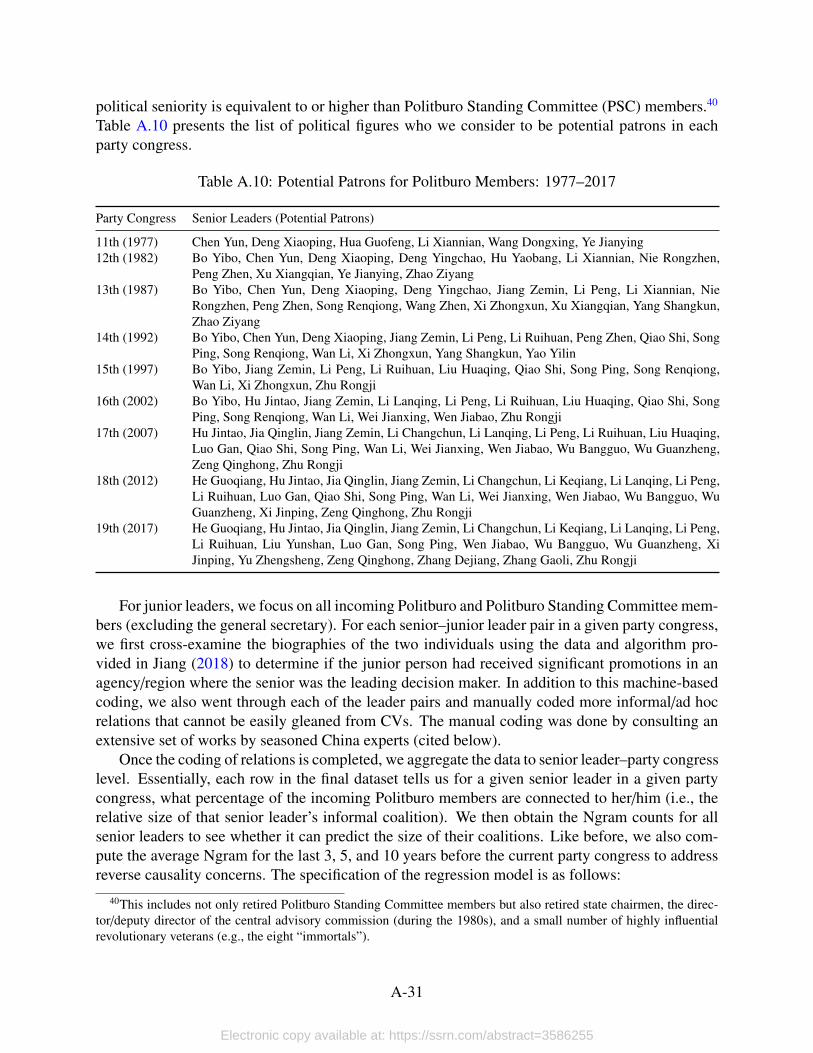
political seniority is equivalent to or higher than Politburo Standing Committee (PSC) members.40

Table A.10 presents the list of political figures who we consider to be potential patrons in eachparty congress.

Table A.10: Potential Patrons for Politburo Members: 1977–2017

Party Congress Senior Leaders (Potential Patrons)

11th (1977) Chen Yun, Deng Xiaoping, Hua Guofeng, Li Xiannian, Wang Dongxing, Ye Jianying12th (1982) Bo Yibo, Chen Yun, Deng Xiaoping, Deng Yingchao, Hu Yaobang, Li Xiannian, Nie Rongzhen,

Peng Zhen, Xu Xiangqian, Ye Jianying, Zhao Ziyang13th (1987) Bo Yibo, Chen Yun, Deng Xiaoping, Deng Yingchao, Jiang Zemin, Li Peng, Li Xiannian, Nie

Rongzhen, Peng Zhen, Song Renqiong, Wang Zhen, Xi Zhongxun, Xu Xiangqian, Yang Shangkun,Zhao Ziyang

14th (1992) Bo Yibo, Chen Yun, Deng Xiaoping, Jiang Zemin, Li Peng, Li Ruihuan, Peng Zhen, Qiao Shi, SongPing, Song Renqiong, Wan Li, Xi Zhongxun, Yang Shangkun, Yao Yilin

15th (1997) Bo Yibo, Jiang Zemin, Li Peng, Li Ruihuan, Liu Huaqing, Qiao Shi, Song Ping, Song Renqiong,Wan Li, Xi Zhongxun, Zhu Rongji

16th (2002) Bo Yibo, Hu Jintao, Jiang Zemin, Li Lanqing, Li Peng, Li Ruihuan, Liu Huaqing, Qiao Shi, SongPing, Song Renqiong, Wan Li, Wei Jianxing, Wen Jiabao, Zhu Rongji

17th (2007) Hu Jintao, Jia Qinglin, Jiang Zemin, Li Changchun, Li Lanqing, Li Peng, Li Ruihuan, Liu Huaqing,Luo Gan, Qiao Shi, Song Ping, Wan Li, Wei Jianxing, Wen Jiabao, Wu Bangguo, Wu Guanzheng,Zeng Qinghong, Zhu Rongji

18th (2012) He Guoqiang, Hu Jintao, Jia Qinglin, Jiang Zemin, Li Changchun, Li Keqiang, Li Lanqing, Li Peng,Li Ruihuan, Luo Gan, Qiao Shi, Song Ping, Wan Li, Wei Jianxing, Wen Jiabao, Wu Bangguo, WuGuanzheng, Xi Jinping, Zeng Qinghong, Zhu Rongji

19th (2017) He Guoqiang, Hu Jintao, Jia Qinglin, Jiang Zemin, Li Changchun, Li Keqiang, Li Lanqing, Li Peng,Li Ruihuan, Liu Yunshan, Luo Gan, Song Ping, Wen Jiabao, Wu Bangguo, Wu Guanzheng, XiJinping, Yu Zhengsheng, Zeng Qinghong, Zhang Dejiang, Zhang Gaoli, Zhu Rongji

For junior leaders, we focus on all incoming Politburo and Politburo Standing Committee mem-bers (excluding the general secretary). For each senior–junior leader pair in a given party congress,we first cross-examine the biographies of the two individuals using the data and algorithm pro-vided in Jiang (2018) to determine if the junior person had received significant promotions in anagency/region where the senior was the leading decision maker. In addition to this machine-basedcoding, we also went through each of the leader pairs and manually coded more informal/ad hocrelations that cannot be easily gleaned from CVs. The manual coding was done by consulting anextensive set of works by seasoned China experts (cited below).

Once the coding of relations is completed, we aggregate the data to senior leader–party congresslevel. Essentially, each row in the final dataset tells us for a given senior leader in a given partycongress, what percentage of the incoming Politburo members are connected to her/him (i.e., therelative size of that senior leader’s informal coalition). We then obtain the Ngram counts for allsenior leaders to see whether it can predict the size of their coalitions. Like before, we also com-pute the average Ngram for the last 3, 5, and 10 years before the current party congress to addressreverse causality concerns. The specification of the regression model is as follows:

40This includes not only retired Politburo Standing Committee members but also retired state chairmen, the direc-tor/deputy director of the central advisory commission (during the 1980s), and a small number of highly influentialrevolutionary veterans (e.g., the eight “immortals”).

A-31


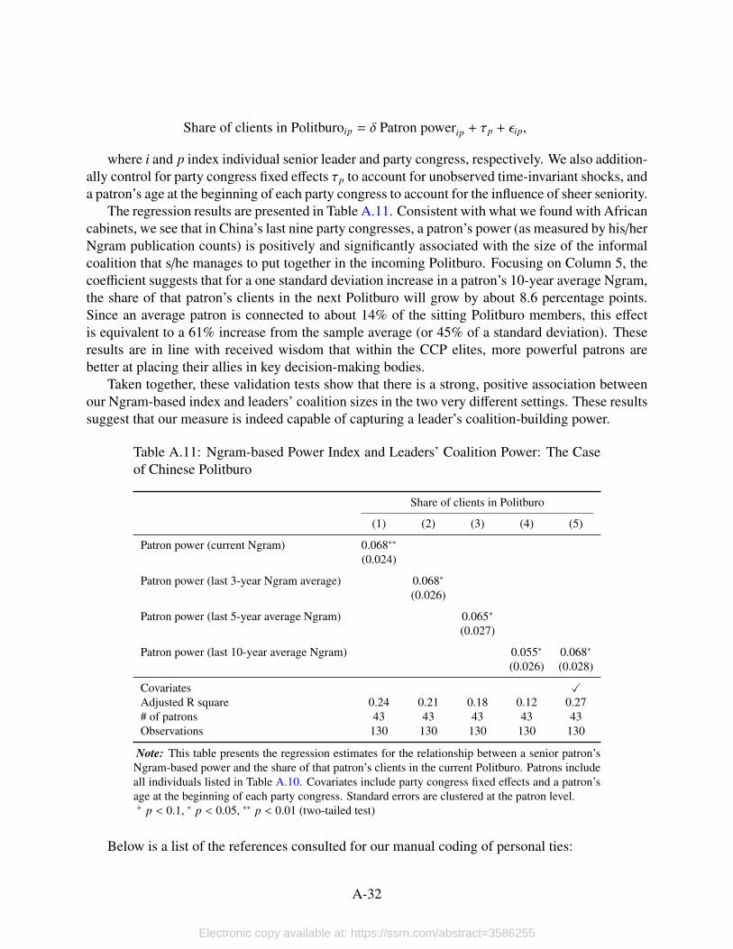
Share of clients in Politburoip = δ Patron powerip + τp + εip,

where i and p index individual senior leader and party congress, respectively. We also addition-ally control for party congress fixed effects τp to account for unobserved time-invariant shocks, anda patron’s age at the beginning of each party congress to account for the influence of sheer seniority.

The regression results are presented in Table A.11. Consistent with what we found with Africancabinets, we see that in China’s last nine party congresses, a patron’s power (as measured by his/herNgram publication counts) is positively and significantly associated with the size of the informalcoalition that s/he manages to put together in the incoming Politburo. Focusing on Column 5, thecoefficient suggests that for a one standard deviation increase in a patron’s 10-year average Ngram,the share of that patron’s clients in the next Politburo will grow by about 8.6 percentage points.Since an average patron is connected to about 14% of the sitting Politburo members, this effectis equivalent to a 61% increase from the sample average (or 45% of a standard deviation). Theseresults are in line with received wisdom that within the CCP elites, more powerful patrons arebetter at placing their allies in key decision-making bodies.

Taken together, these validation tests show that there is a strong, positive association betweenour Ngram-based index and leaders’ coalition sizes in the two very different settings. These resultssuggest that our measure is indeed capable of capturing a leader’s coalition-building power.

Table A.11: Ngram-based Power Index and Leaders’ Coalition Power: The Caseof Chinese Politburo

Share of clients in Politburo

(1) (2) (3) (4) (5)

Patron power (current Ngram) 0.068∗∗

(0.024)

Patron power (last 3-year Ngram average) 0.068∗

(0.026)

Patron power (last 5-year average Ngram) 0.065∗

(0.027)

Patron power (last 10-year average Ngram) 0.055∗ 0.068∗

(0.026) (0.028)

Covariates XAdjusted R square 0.24 0.21 0.18 0.12 0.27# of patrons 43 43 43 43 43Observations 130 130 130 130 130

Note: This table presents the regression estimates for the relationship between a senior patron’sNgram-based power and the share of that patron’s clients in the current Politburo. Patrons includeall individuals listed in Table A.10. Covariates include party congress fixed effects and a patron’sage at the beginning of each party congress. Standard errors are clustered at the patron level.+ p < 0.1, ∗ p < 0.05, ∗∗ p < 0.01 (two-tailed test)

Below is a list of the references consulted for our manual coding of personal ties:

A-32


• Lowell Dittmer. 2020. “On the Sixth Generation: Preliminary Speculations about ChinesePolitics after Xi.” Journal of Contemporary China 29 (122): 253–265

• Dorothy Grouse Fontana. 1982. “Background to the Fall of Hua Guofeng.” Asian Survey 22(3): 237–260

• Jing Huang. 2000. Factionalism in Chinese Communist Politics. Cambridge University Press

• Chien-wen Kou. 2017. “Xi Jinping in Command: Solving the Principal–Agent Problem inCCP–PLA Relations?” The China Quarterly 232:866–885

• Willy Lam. 2006. Chinese Politics in the Hu Jintao Era : New Leaders, New Challenges.Armonk, N.Y: M.E. Sharpe

• David Lampton. 2013. Following the leader : ruling China, from Deng Xiaoping to Xi Jin-ping. Berkeley: University of California Press

• Cheng Li and Lynn White. 1998. “The Fifteenth Central Committee of the Chinese Com-munist Party: Full-Fledged Technocratic Leadership with Partial Control by Jiang Zemin.”Asian Survey 38 (3): 231–264

• Cheng Li. 2002. “Hu’s Followers:Provincial Leaders with Backgrounds in the Youth League.”China Leadership Monitor 3:1–11

• Cheng Li. 2007. “Was the Shanghai Gang Shanghaied?” China Leadership Monitor, no. 20

• Cheng Li. 2012. “The Battle for China’s TopNine Leadership Posts.” The Washington Quar-terly 35 (1): 131–145

• Cheng Li. 2016. Chinese Politics in the Xi Jinping Era: Reassessing Collective Leadership.Brookings Institution Press

• Ezra Vogel. 2013. Deng Xiaoping and the Transformation of China. Belknap Press of Har-vard University Press

• Ziyang Zhao. 2009. Prisoner of the State: The Secret Journal of Premier Zhao Ziyang. Simon& Schuster

• 杨继绳. (2004).中国改革年代的政治斗争.香港：天地图书有限公司

• “The Committee”, Marco Polo, https://macropolo.org/digital-projects/the-committee/

• “Connected China”, Reuters, http://china.fathom.info/

A-33


https://macropolo.org/digital-projects/the-committee/

http://china.fathom.info/

C.8 Correlation with Existing Power Measures

Table A.12: Correlation between Ngram-based Power Index and GWF Personalismat t

DV: Personalism index (GWF)

(1) (2) (3) (4) (5) (6)

Incumbent’s Ngram at t + 2 0.197∗∗∗ 0.031(0.008) (0.006)

Incumbent’s Ngram at t + 1 0.234∗∗∗ 0.035(0.008) (0.005)

Incumbent’s Ngram at t 0.273∗∗∗ 0.175∗∗∗

(0.009) (0.007)

Incumbent’s Ngram at t − 1 0.240∗∗∗ 0.059∗∗∗

(0.009) (0.004)

Incumbent’s Ngram at t − 2 0.198∗∗∗ 0.005(0.009) (0.007)

Country and year fixed effects X X X X XAdjusted R2 0.61 0.62 0.62 0.62 0.61 0.62Observations 3934 3934 3934 3934 3934 3934

Note: This table presents the standardized regression coefficients for the relationship between ourNgram-based power index and the personalism index developed by Geddes, Wright, and Frantz(2019). Standard errors are clustered at country level.+ p < 0.1, ∗ p < 0.05, ∗∗ p < 0.01 (two-tailed test)

A-34


Table A.13: Correlation between Ngram-based Power Index and Power Con-solidation Index

DV: Power consolidation measure (GS)

(1) (2) (3) (4) (5) (6)

Incumbent’s Ngram at t + 2 0.059 0.052∗

(0.043) (0.025)

Incumbent’s Ngram at t + 1 0.049 0.008(0.045) (0.012)

Incumbent’s Ngram at t 0.038 -0.032(0.047) (0.019)

Incumbent’s Ngram at t − 1 0.045 0.008(0.045) (0.014)

Incumbent’s Ngram at t − 2 0.051 0.037(0.044) (0.026)

Country and year fixed effects X X X X XAdjusted R2 0.72 0.72 0.72 0.72 0.72 0.72Observations 4254 4254 4254 4254 4254 4254

Note: This table presents the standardized regression coefficients for the relationship betweenour Ngram-based power index and the power consolidation measure developed by Gandhi andSumner (2020). Standard errors are clustered at country level.+ p < 0.1, ∗ p < 0.05, ∗∗ p < 0.01 (two-tailed test)

A-35


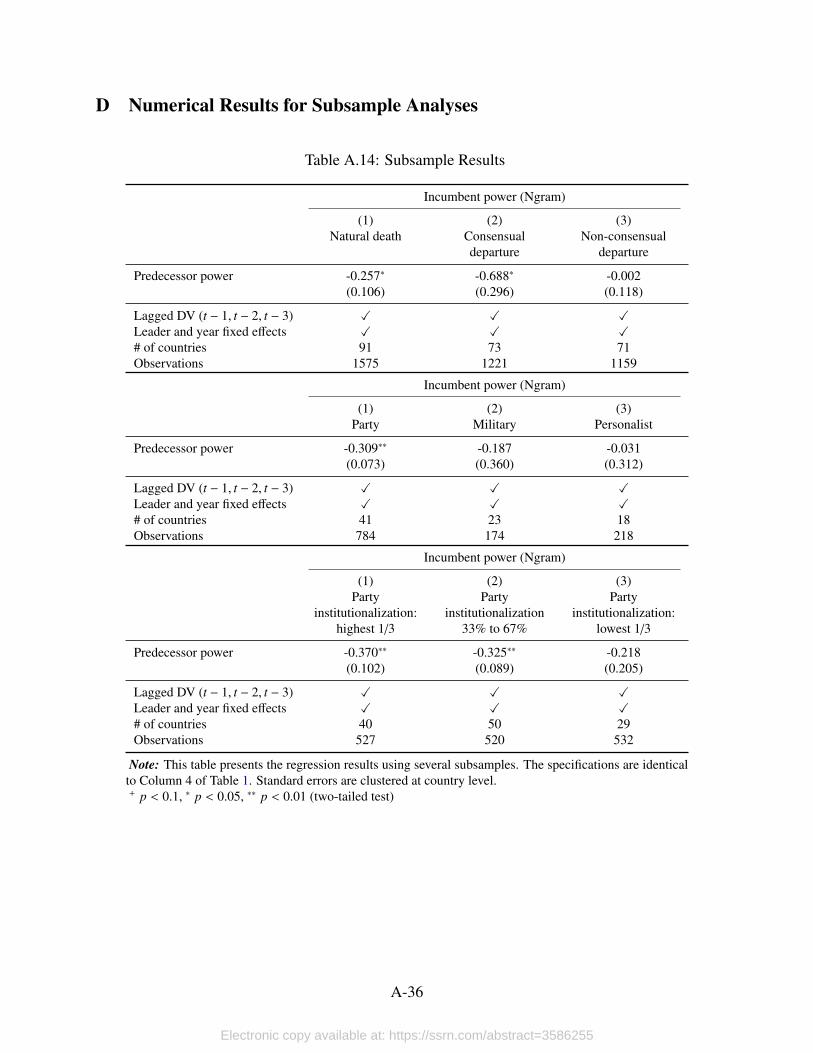
D Numerical Results for Subsample Analyses

Table A.14: Subsample Results

Incumbent power (Ngram)

(1) (2) (3)Natural death Consensual

departureNon-consensual

departure

Predecessor power -0.257∗ -0.688∗ -0.002(0.106) (0.296) (0.118)

Lagged DV (t − 1, t − 2, t − 3) X X XLeader and year fixed effects X X X# of countries 91 73 71Observations 1575 1221 1159


(1) (2) (3)Party Military Personalist

Predecessor power -0.309∗∗ -0.187 -0.031(0.073) (0.360) (0.312)



(1) (2) (3)Party

institutionalization:highest 1/3

Partyinstitutionalization

33% to 67%

Partyinstitutionalization:

lowest 1/3

Predecessor power -0.370∗∗ -0.325∗∗ -0.218(0.102) (0.089) (0.205)


Note: This table presents the regression results using several subsamples. The specifications are identicalto Column 4 of Table 1. Standard errors are clustered at country level.+ p < 0.1, ∗ p < 0.05, ∗∗ p < 0.01 (two-tailed test)

A-36


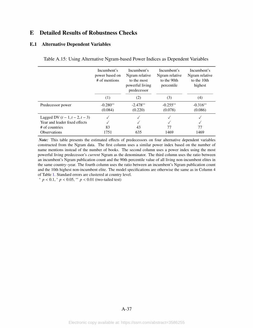
E Detailed Results of Robustness Checks

E.1 Alternative Dependent Variables

Table A.15: Using Alternative Ngram-based Power Indices as Dependent Variables

Incumbent’spower based on# of mentions

Incumbent’sNgram relative

to the mostpowerful living

predecessor


to the 90thpercentile


to the 10thhighest

(1) (2) (3) (4)

Predecessor power -0.280∗∗ -2.478∗∗ -0.255∗∗ -0.316∗∗

(0.084) (0.220) (0.078) (0.086)

Lagged DV (t − 1, t − 2, t − 3) X X X XYear and leader fixed effects X X X X# of countries 83 43 77 77Observations 1751 635 1469 1469

Note: This table presents the estimated effects of predecessors on four alternative dependent variablesconstructed from the Ngram data. The first column uses a similar power index based on the number ofname mentions instead of the number of books. The second column uses a power index using the mostpowerful living predecessor’s current Ngram as the denominator. The third column uses the ratio betweenan incumbent’s Ngram publication count and the 90th percentile value of all living non-incumbent elites inthe same country–year. The fourth column uses the ratio between an incumbent’s Ngram publication countand the 10th highest non-incumbent elite. The model specifications are otherwise the same as in Column 4of Table 1. Standard errors are clustered at country level.+ p < 0.1, ∗ p < 0.05, ∗∗ p < 0.01 (two-tailed test)

A-37


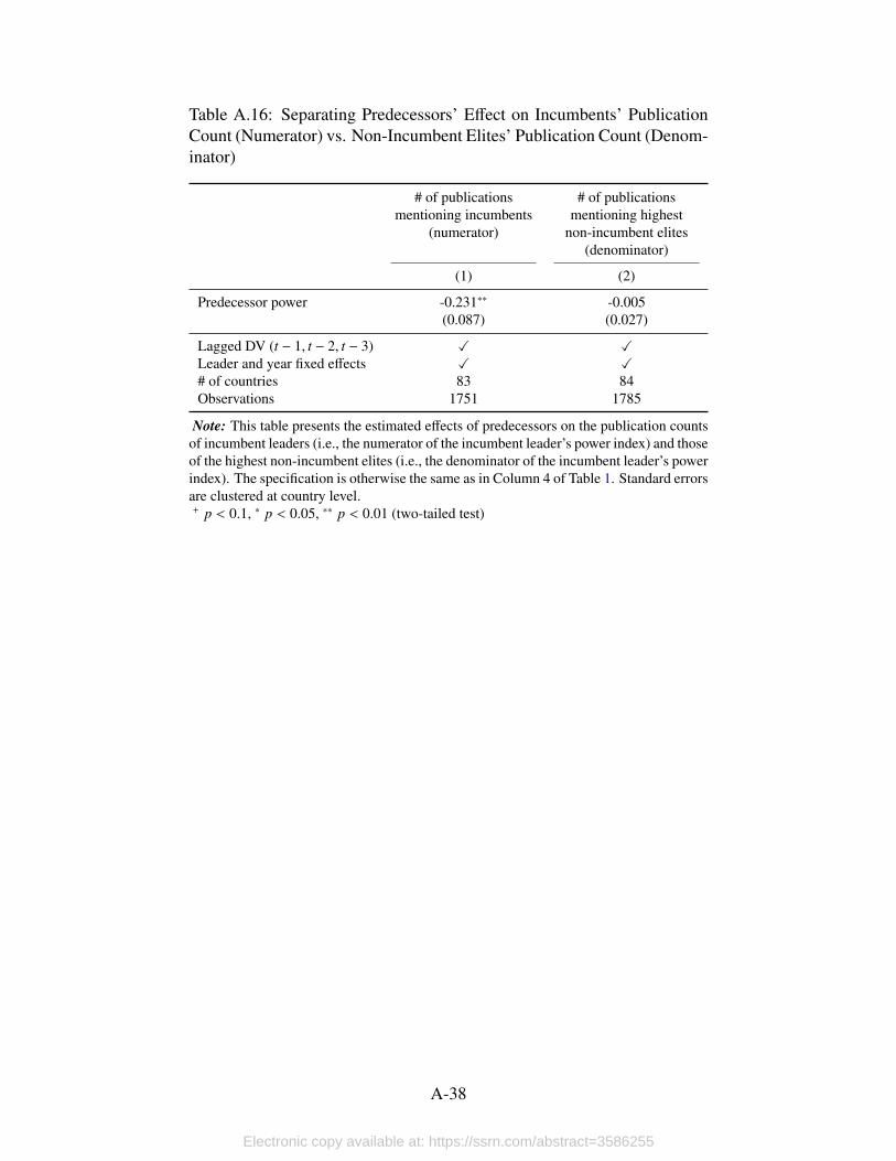
Table A.16: Separating Predecessors’ Effect on Incumbents’ PublicationCount (Numerator) vs. Non-Incumbent Elites’ Publication Count (Denom-inator)

# of publicationsmentioning incumbents

(numerator)

# of publicationsmentioning highest

non-incumbent elites(denominator)

(1) (2)

Predecessor power -0.231∗∗ -0.005(0.087) (0.027)

Lagged DV (t − 1, t − 2, t − 3) X XLeader and year fixed effects X X# of countries 83 84Observations 1751 1785

Note: This table presents the estimated effects of predecessors on the publication countsof incumbent leaders (i.e., the numerator of the incumbent leader’s power index) and thoseof the highest non-incumbent elites (i.e., the denominator of the incumbent leader’s powerindex). The specification is otherwise the same as in Column 4 of Table 1. Standard errorsare clustered at country level.+ p < 0.1, ∗ p < 0.05, ∗∗ p < 0.01 (two-tailed test)

A-38


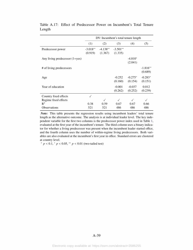
Table A.17: Effect of Predecessor Power on Incumbent’s Total TenureLength

DV: Incumbent’s total tenure length

(1) (2) (3) (4) (5)

Predecessor power -3.018∗∗ -4.138∗∗ -3.501∗∗

(0.919) (1.367) (1.335)

Any living predecessor (1=yes) -4.810∗

(2.041)

# of living predecessors -1.816∗∗

(0.689)

Age -0.252 -0.275+ -0.283+

(0.160) (0.154) (0.151)

Year of education -0.001 -0.037 0.012(0.262) (0.252) (0.239)

Country fixed effects XRegime fixed effects X X X XR2 0.38 0.59 0.67 0.67 0.66Observations 521 521 486 486 486

Note: This table presents the regression results using incumbent leaders’ total tenurelength as the alternative outcome. The analysis is at individual leader level. The key inde-pendent variable for the first two columns is the predecessor power index used in Table 1,evaluated at the first year of the incumbent’s tenure. The third column uses a binary indica-tor for whether a living predecessor was present when the incumbent leader started office,and the fourth column uses the number of within-regime living predecessors. Both vari-ables are also evaluated at the incumbent’s first year in office. Standard errors are clusteredat country level.+ p < 0.1, ∗ p < 0.05, ∗∗ p < 0.01 (two-tailed test)

A-39


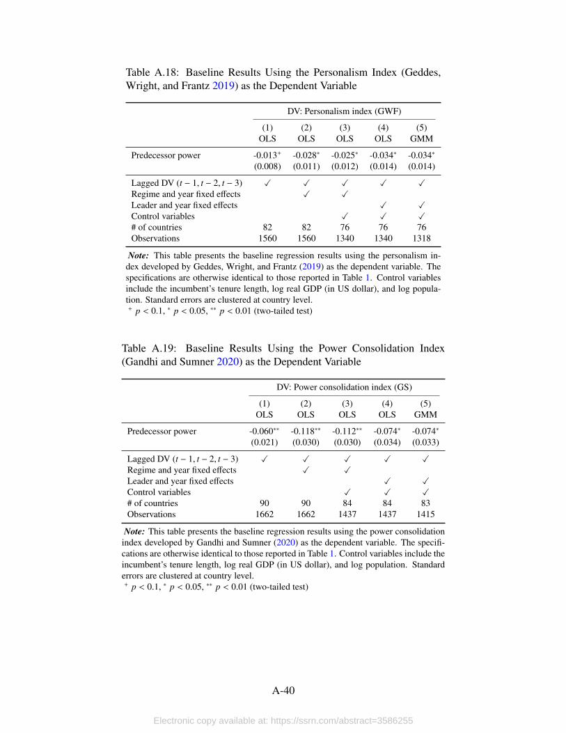
Table A.18: Baseline Results Using the Personalism Index (Geddes,Wright, and Frantz 2019) as the Dependent Variable

DV: Personalism index (GWF)


Predecessor power -0.013+ -0.028∗ -0.025∗ -0.034∗ -0.034∗

(0.008) (0.011) (0.012) (0.014) (0.014)


Note: This table presents the baseline regression results using the personalism in-dex developed by Geddes, Wright, and Frantz (2019) as the dependent variable. Thespecifications are otherwise identical to those reported in Table 1. Control variablesinclude the incumbent’s tenure length, log real GDP (in US dollar), and log popula-tion. Standard errors are clustered at country level.+ p < 0.1, ∗ p < 0.05, ∗∗ p < 0.01 (two-tailed test)

Table A.19: Baseline Results Using the Power Consolidation Index(Gandhi and Sumner 2020) as the Dependent Variable

DV: Power consolidation index (GS)


Predecessor power -0.060∗∗ -0.118∗∗ -0.112∗∗ -0.074∗ -0.074∗

(0.021) (0.030) (0.030) (0.034) (0.033)


Note: This table presents the baseline regression results using the power consolidationindex developed by Gandhi and Sumner (2020) as the dependent variable. The specifi-cations are otherwise identical to those reported in Table 1. Control variables include theincumbent’s tenure length, log real GDP (in US dollar), and log population. Standarderrors are clustered at country level.+ p < 0.1, ∗ p < 0.05, ∗∗ p < 0.01 (two-tailed test)

A-40


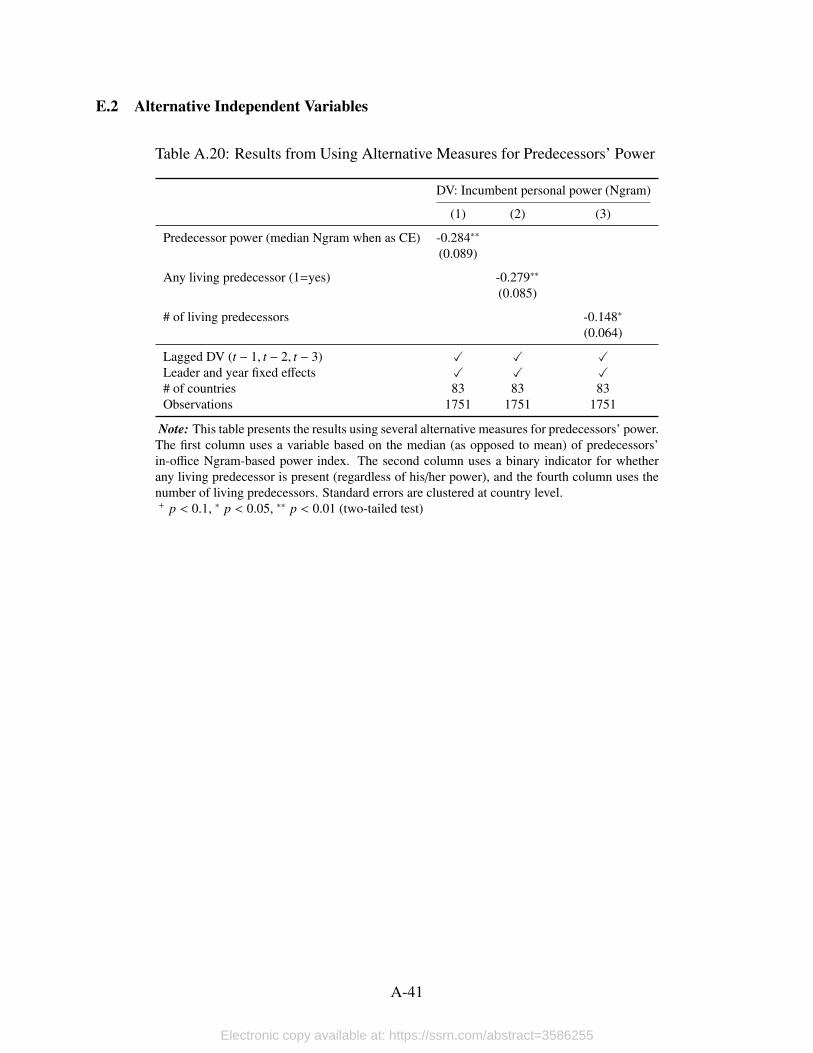
E.2 Alternative Independent Variables

Table A.20: Results from Using Alternative Measures for Predecessors’ Power

DV: Incumbent personal power (Ngram)

(1) (2) (3)

Predecessor power (median Ngram when as CE) -0.284∗∗

(0.089)

Any living predecessor (1=yes) -0.279∗∗

(0.085)

# of living predecessors -0.148∗

(0.064)


Note: This table presents the results using several alternative measures for predecessors’ power.The first column uses a variable based on the median (as opposed to mean) of predecessors’in-office Ngram-based power index. The second column uses a binary indicator for whetherany living predecessor is present (regardless of his/her power), and the fourth column uses thenumber of living predecessors. Standard errors are clustered at country level.+ p < 0.1, ∗ p < 0.05, ∗∗ p < 0.01 (two-tailed test)

A-41


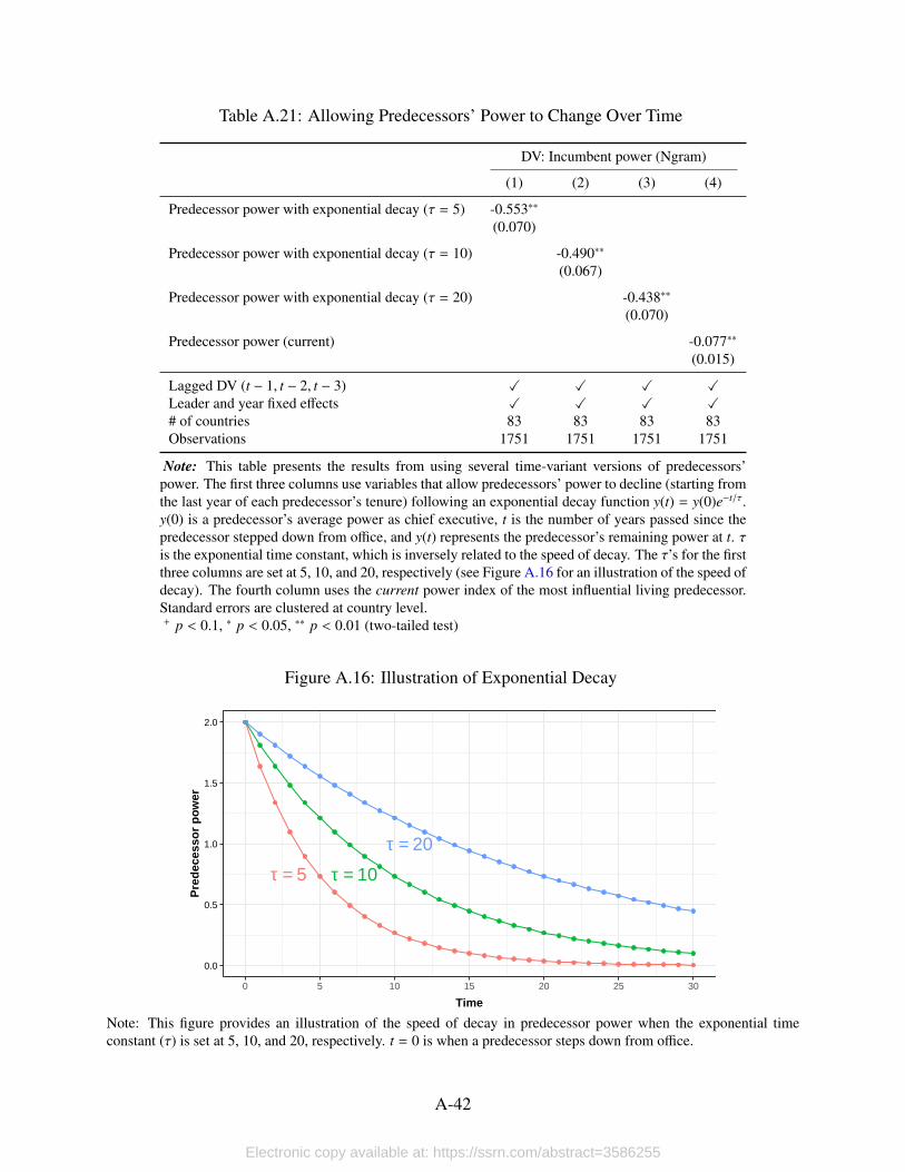
Table A.21: Allowing Predecessors’ Power to Change Over Time

DV: Incumbent power (Ngram)

(1) (2) (3) (4)

Predecessor power with exponential decay (τ = 5) -0.553∗∗

(0.070)


(0.067)


(0.070)

Predecessor power (current) -0.077∗∗

(0.015)

Lagged DV (t − 1, t − 2, t − 3) X X X XLeader and year fixed effects X X X X# of countries 83 83 83 83Observations 1751 1751 1751 1751

Note: This table presents the results from using several time-variant versions of predecessors’power. The first three columns use variables that allow predecessors’ power to decline (starting fromthe last year of each predecessor’s tenure) following an exponential decay function y(t) = y(0)e−t/τ.y(0) is a predecessor’s average power as chief executive, t is the number of years passed since thepredecessor stepped down from office, and y(t) represents the predecessor’s remaining power at t. τis the exponential time constant, which is inversely related to the speed of decay. The τ’s for the firstthree columns are set at 5, 10, and 20, respectively (see Figure A.16 for an illustration of the speed ofdecay). The fourth column uses the current power index of the most influential living predecessor.Standard errors are clustered at country level.+ p < 0.1, ∗ p < 0.05, ∗∗ p < 0.01 (two-tailed test)

Figure A.16: Illustration of Exponential Decay

τ = 5 τ = 10

τ = 20

0.0

0.5

1.0

1.5

2.0

0 5 10 15 20 25 30

Time

Pre

dece

ssor

pow

er

Note: This figure provides an illustration of the speed of decay in predecessor power when the exponential timeconstant (τ) is set at 5, 10, and 20, respectively. t = 0 is when a predecessor steps down from office.

A-42


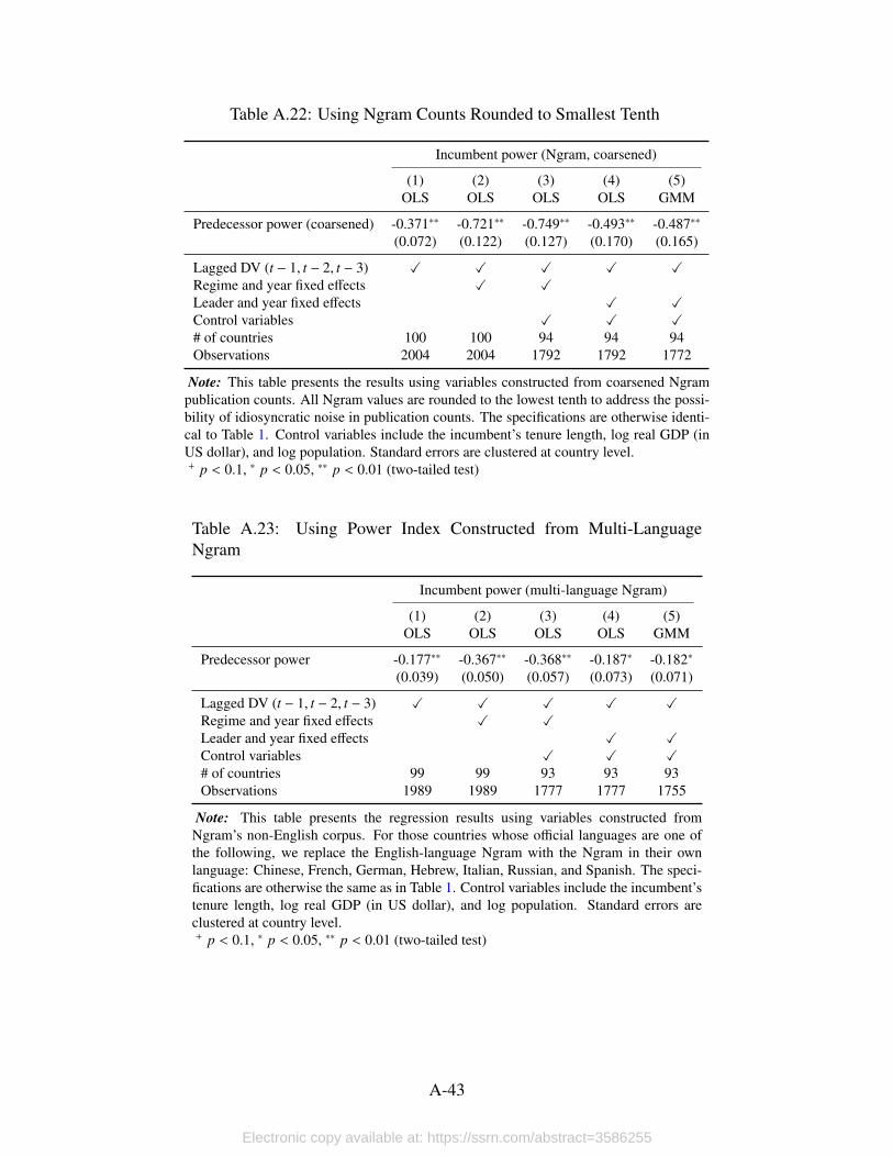
Table A.22: Using Ngram Counts Rounded to Smallest Tenth

Incumbent power (Ngram, coarsened)


Predecessor power (coarsened) -0.371∗∗ -0.721∗∗ -0.749∗∗ -0.493∗∗ -0.487∗∗

(0.072) (0.122) (0.127) (0.170) (0.165)


Note: This table presents the results using variables constructed from coarsened Ngrampublication counts. All Ngram values are rounded to the lowest tenth to address the possi-bility of idiosyncratic noise in publication counts. The specifications are otherwise identi-cal to Table 1. Control variables include the incumbent’s tenure length, log real GDP (inUS dollar), and log population. Standard errors are clustered at country level.+ p < 0.1, ∗ p < 0.05, ∗∗ p < 0.01 (two-tailed test)

Table A.23: Using Power Index Constructed from Multi-LanguageNgram

Incumbent power (multi-language Ngram)



(0.039) (0.050) (0.057) (0.073) (0.071)


Note: This table presents the regression results using variables constructed fromNgram’s non-English corpus. For those countries whose official languages are one ofthe following, we replace the English-language Ngram with the Ngram in their ownlanguage: Chinese, French, German, Hebrew, Italian, Russian, and Spanish. The speci-fications are otherwise the same as in Table 1. Control variables include the incumbent’stenure length, log real GDP (in US dollar), and log population. Standard errors areclustered at country level.+ p < 0.1, ∗ p < 0.05, ∗∗ p < 0.01 (two-tailed test)

A-43


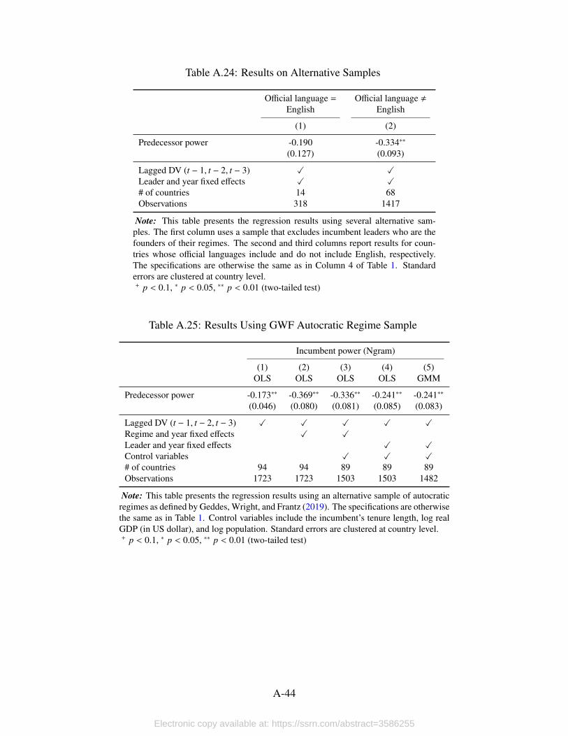
Table A.24: Results on Alternative Samples

Official language =

EnglishOfficial language ,

English

(1) (2)

Predecessor power -0.190 -0.334∗∗

(0.127) (0.093)

Lagged DV (t − 1, t − 2, t − 3) X XLeader and year fixed effects X X# of countries 14 68Observations 318 1417

Note: This table presents the regression results using several alternative sam-ples. The first column uses a sample that excludes incumbent leaders who are thefounders of their regimes. The second and third columns report results for coun-tries whose official languages include and do not include English, respectively.The specifications are otherwise the same as in Column 4 of Table 1. Standarderrors are clustered at country level.+ p < 0.1, ∗ p < 0.05, ∗∗ p < 0.01 (two-tailed test)

Table A.25: Results Using GWF Autocratic Regime Sample



Predecessor power -0.173∗∗ -0.369∗∗ -0.336∗∗ -0.241∗∗ -0.241∗∗

(0.046) (0.080) (0.081) (0.085) (0.083)


Note: This table presents the regression results using an alternative sample of autocraticregimes as defined by Geddes, Wright, and Frantz (2019). The specifications are otherwisethe same as in Table 1. Control variables include the incumbent’s tenure length, log realGDP (in US dollar), and log population. Standard errors are clustered at country level.+ p < 0.1, ∗ p < 0.05, ∗∗ p < 0.01 (two-tailed test)

A-44


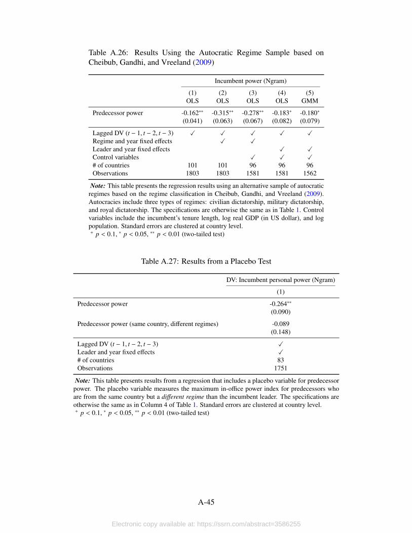
Table A.26: Results Using the Autocratic Regime Sample based onCheibub, Gandhi, and Vreeland (2009)




(0.041) (0.063) (0.067) (0.082) (0.079)


Note: This table presents the regression results using an alternative sample of autocraticregimes based on the regime classification in Cheibub, Gandhi, and Vreeland (2009).Autocracies include three types of regimes: civilian dictatorship, military dictatorship,and royal dictatorship. The specifications are otherwise the same as in Table 1. Controlvariables include the incumbent’s tenure length, log real GDP (in US dollar), and logpopulation. Standard errors are clustered at country level.+ p < 0.1, ∗ p < 0.05, ∗∗ p < 0.01 (two-tailed test)

Table A.27: Results from a Placebo Test

DV: Incumbent personal power (Ngram)

(1)

Predecessor power -0.264∗∗

(0.090)

Predecessor power (same country, different regimes) -0.089(0.148)

Lagged DV (t − 1, t − 2, t − 3) XLeader and year fixed effects X# of countries 83Observations 1751

Note: This table presents results from a regression that includes a placebo variable for predecessorpower. The placebo variable measures the maximum in-office power index for predecessors whoare from the same country but a different regime than the incumbent leader. The specifications areotherwise the same as in Column 4 of Table 1. Standard errors are clustered at country level.+ p < 0.1, ∗ p < 0.05, ∗∗ p < 0.01 (two-tailed test)

A-45


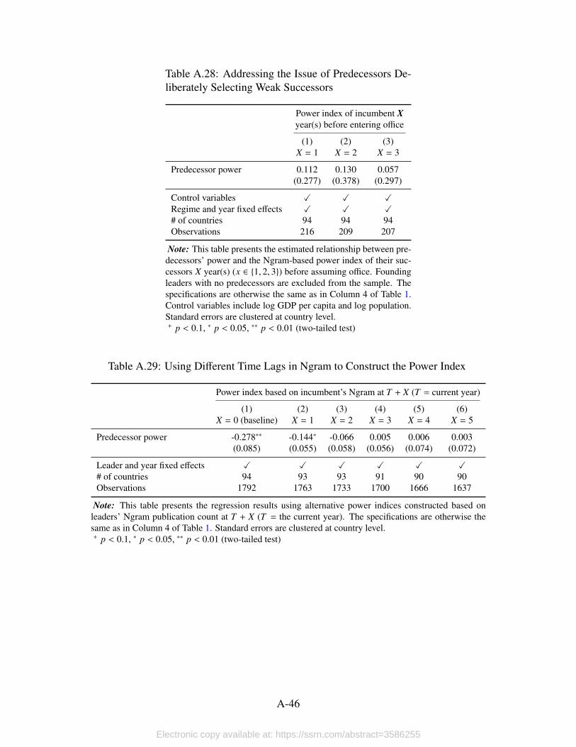
Table A.28: Addressing the Issue of Predecessors De-liberately Selecting Weak Successors

Power index of incumbent Xyear(s) before entering office

(1) (2) (3)X = 1 X = 2 X = 3

Predecessor power 0.112 0.130 0.057(0.277) (0.378) (0.297)

Control variables X X XRegime and year fixed effects X X X# of countries 94 94 94Observations 216 209 207

Note: This table presents the estimated relationship between pre-decessors’ power and the Ngram-based power index of their suc-cessors X year(s) (x ∈ {1, 2, 3}) before assuming office. Foundingleaders with no predecessors are excluded from the sample. Thespecifications are otherwise the same as in Column 4 of Table 1.Control variables include log GDP per capita and log population.Standard errors are clustered at country level.+ p < 0.1, ∗ p < 0.05, ∗∗ p < 0.01 (two-tailed test)

Table A.29: Using Different Time Lags in Ngram to Construct the Power Index

Power index based on incumbent’s Ngram at T + X (T = current year)

(1) (2) (3) (4) (5) (6)X = 0 (baseline) X = 1 X = 2 X = 3 X = 4 X = 5

Predecessor power -0.278∗∗ -0.144∗ -0.066 0.005 0.006 0.003(0.085) (0.055) (0.058) (0.056) (0.074) (0.072)

Leader and year fixed effects X X X X X X# of countries 94 93 93 91 90 90Observations 1792 1763 1733 1700 1666 1637

Note: This table presents the regression results using alternative power indices constructed based onleaders’ Ngram publication count at T + X (T = the current year). The specifications are otherwise thesame as in Column 4 of Table 1. Standard errors are clustered at country level.+ p < 0.1, ∗ p < 0.05, ∗∗ p < 0.01 (two-tailed test)

A-46


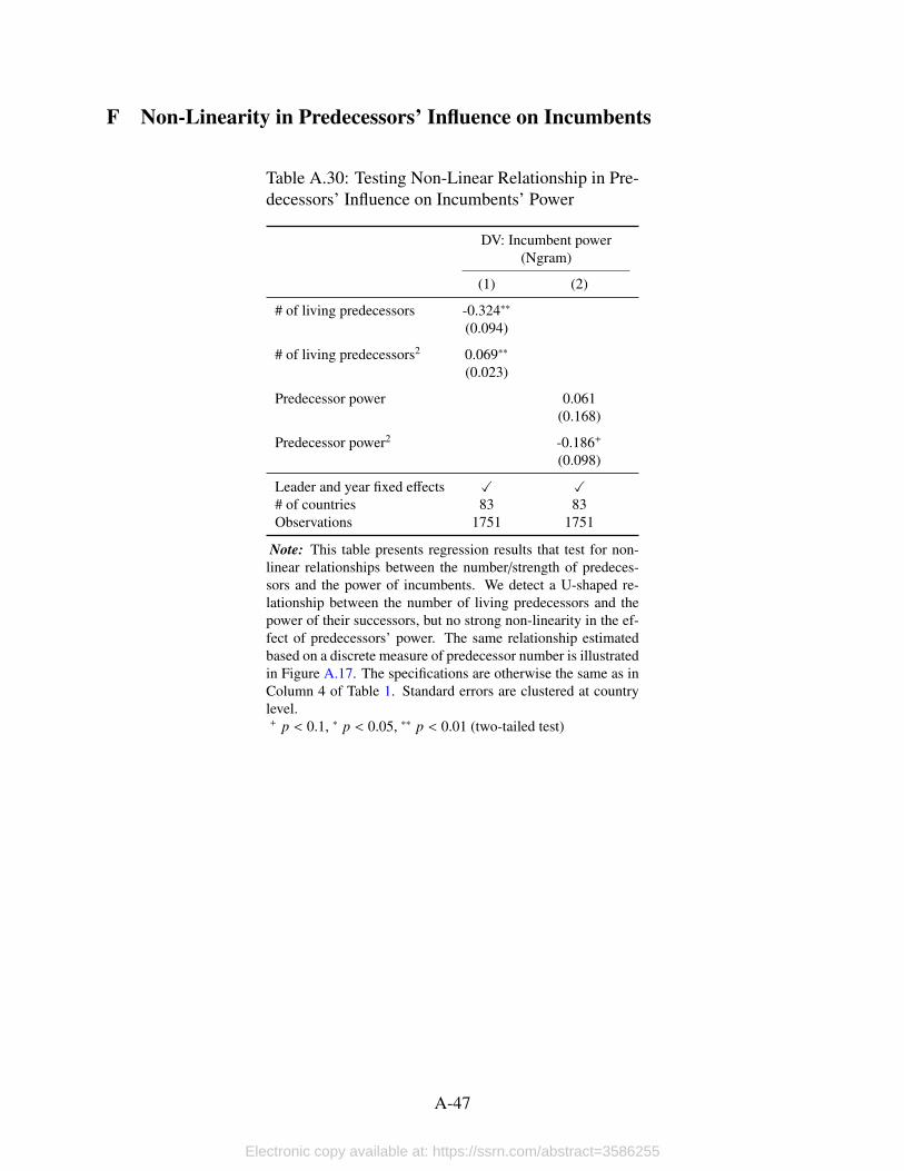
F Non-Linearity in Predecessors’ Influence on Incumbents

Table A.30: Testing Non-Linear Relationship in Pre-decessors’ Influence on Incumbents’ Power

DV: Incumbent power(Ngram)

(1) (2)

# of living predecessors -0.324∗∗

(0.094)

# of living predecessors2 0.069∗∗

(0.023)

Predecessor power 0.061(0.168)

Predecessor power2 -0.186+

(0.098)

Leader and year fixed effects X X# of countries 83 83Observations 1751 1751

Note: This table presents regression results that test for non-linear relationships between the number/strength of predeces-sors and the power of incumbents. We detect a U-shaped re-lationship between the number of living predecessors and thepower of their successors, but no strong non-linearity in the ef-fect of predecessors’ power. The same relationship estimatedbased on a discrete measure of predecessor number is illustratedin Figure A.17. The specifications are otherwise the same as inColumn 4 of Table 1. Standard errors are clustered at countrylevel.+ p < 0.1, ∗ p < 0.05, ∗∗ p < 0.01 (two-tailed test)

A-47


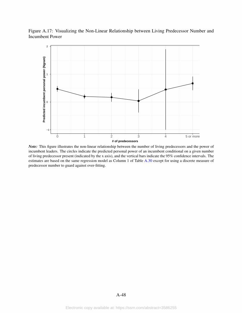
Figure A.17: Visualizing the Non-Linear Relationship between Living Predecessor Number andIncumbent Power

−1

0

1

2

0 1 2 3 4 5 or more# of predecessors

Pre

dict

ed in

cum

bent

per

sona

l pow

er (

Ngr

am)

Note: This figure illustrates the non-linear relationship between the number of living predecessors and the power ofincumbent leaders. The circles indicate the predicted personal power of an incumbent conditional on a given numberof living predecessor present (indicated by the x axis), and the vertical bars indicate the 95% confidence intervals. Theestimates are based on the same regression model as Column 1 of Table A.30 except for using a discrete measure ofpredecessor number to guard against over-fitting.

A-48


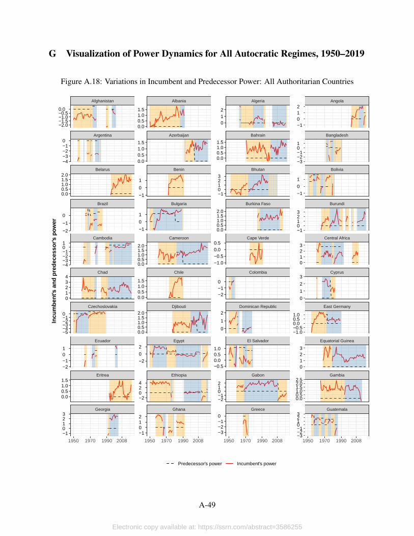
G Visualization of Power Dynamics for All Autocratic Regimes, 1950–2019

Figure A.18: Variations in Incumbent and Predecessor Power: All Authoritarian Countries

Georgia Ghana Greece Guatemala

Eritrea Ethiopia Gabon Gambia

Ecuador Egypt El Salvador Equatorial Guinea

Czechoslovakia Djibouti Dominican Republic East Germany

Chad Chile Colombia Cyprus

Cambodia Cameroon Cape Verde Central Africa

Brazil Bulgaria Burkina Faso Burundi

Belarus Benin Bhutan Bolivia

Argentina Azerbaijan Bahrain Bangladesh

Afghanistan Albania Algeria Angola

1950 1970 1990 2008 1950 1970 1990 2008 1950 1970 1990 2008 1950 1970 1990 2008

−1012

−3−2−101

−1

0

1

−10123

0123

0

1

2

3

−1.0−0.50.00.51.0

0123

0.00.51.01.52.02.5

−3−2−10123

012

0.00.51.01.5

−10123

0.00.51.01.52.0

−1.0−0.50.00.5

−2−10

0

1

2

−0.50.00.51.0

−2−1012

−3−2−10

0.00.51.01.5

0.00.51.01.5

−1

0

1

−1

0

1

0.00.51.01.52.0

0.00.51.01.5

0.00.51.01.52.0

−2

0

2

−2024

−1012

−2.0−1.5−1.0−0.50.0

−4−3−2−10

0.00.51.01.52.0

−2

−1

0

−4−3−2−101

01234

−5−4−3−2−10

−2−101

0.00.51.01.5

−10123

Incu

mbe

nt's

and

pre

dece

ssor

's p

ower


A-49


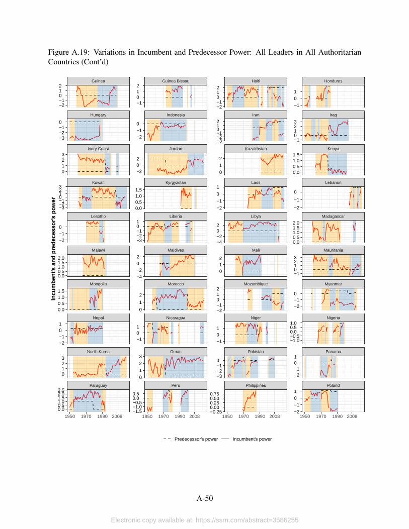
Figure A.19: Variations in Incumbent and Predecessor Power: All Leaders in All AuthoritarianCountries (Cont’d)

Paraguay Peru Philippines Poland

North Korea Oman Pakistan Panama

Nepal Nicaragua Niger Nigeria

Mongolia Morocco Mozambique Myanmar

Malawi Maldives Mali Mauritania

Lesotho Liberia Libya Madagascar

Kuwait Kyrgyzstan Laos Lebanon

Ivory Coast Jordan Kazakhstan Kenya

Hungary Indonesia Iran Iraq

Guinea Guinea Bissau Haiti Honduras

1950 1970 1990 2008 1950 1970 1990 2008 1950 1970 1990 2008 1950 1970 1990 2008

−1

0

1

−10123

0.00.51.01.5

−2

−1

0

0.00.51.01.52.0

−10123

−2−10

−1.0−0.50.00.51.0

−2−101

−2

−1

0

1

−2−1012

−3−2−1012

0

1

2

−2

−1

0

1

−4−202

012

−2−1012

−101

−3−2−10

−0.250.000.250.500.75

−1012

−2−10

−202

0.00.51.01.5

−3−2−101

−4−202

0

1

2

−101

0

1

2

3

−1.5−1.0−0.50.00.5

−2−1012

−3−2−10

0123

−3−2−10123

−2−10

0.00.51.01.52.0

0.00.51.01.5

−2−101

0123

0.00.51.01.52.02.5

Incu

mbe

nt's

and

pre

dece

ssor

's p

ower


A-50


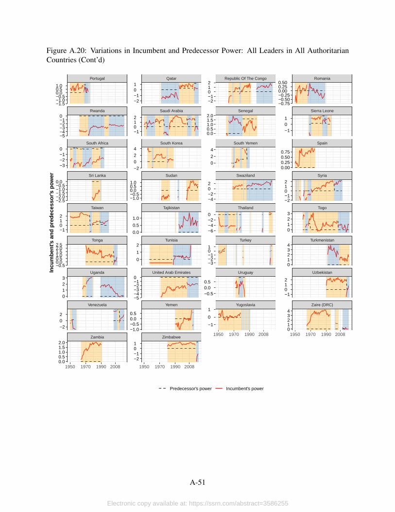
Figure A.20: Variations in Incumbent and Predecessor Power: All Leaders in All AuthoritarianCountries (Cont’d)

Zambia Zimbabwe

Venezuela Yemen Yugoslavia Zaire (DRC)

Uganda United Arab Emirates Uruguay Uzbekistan

Tonga Tunisia Turkey Turkmenistan

Taiwan Tajikistan Thailand Togo

Sri Lanka Sudan Swaziland Syria

South Africa South Korea South Yemen Spain

Rwanda Saudi Arabia Senegal Sierra Leone

Portugal Qatar Republic Of The Congo Romania

1950 1970 1990 2008 1950 1970 1990 2008

1950 1970 1990 2008 1950 1970 1990 2008

−0.75−0.50−0.250.000.250.50

−101

0.000.250.500.75

−2−1012

0123

01234

−1012

01234

−2−1012

0.00.51.01.52.0

0

2

4

−4−202

−6−4−20

−3−2−101

−0.50.00.5

−1

0

1

−2−101

−1012

−2024

−1.0−0.50.00.51.0

0.0

0.5

1.0

0

1

2

−5−4−3−2−10

−1.0−0.50.00.5

−2−101

−1.5−1.0−0.50.00.51.0

−5−4−3−2−10

−3−2−10

−2.5−2.0−1.5−1.0−0.50.0

−1012

−0.50.00.51.01.52.02.5

0123

−202

0.00.51.01.52.0

Incu

mbe

nt's

and

pre

dece

ssor

's p

ower


A-51


References

Arriola, Leonardo R. 2009. “Patronage and Political Stability in Africa.” Comparative PoliticalStudies 42 (10): 1339–1362.

Bates, Robert.H. 1981. Markets and States in Tropical Africa: The Political Basis of AgriculturalPolicies. California series on social choice and political economy. University of CaliforniaPress.

Baturo, Alexander, and Johan A. Elkink. 2014. “Office or Officeholder? Regime Deinstitutional-ization and Sources of Individual Political Influence.” The Journal of Politics 76 (03): 859–872.

Bratton, Michael., and Nicholas. van de Walle. 1997. Democratic Experiments in Africa: RegimeTransitions in Comparative Perspective. Cambridge Studies in Comparative Politics. Cam-bridge University Press.

Castaneda, Jorge.G., and Padraic.A. Smithies. 2001. Perpetuating Power: How Mexican PresidentsWere Chosen. New Press.

Cheibub, Jose Antonio, Jennifer Gandhi, and James Raymond Vreeland. 2009. “Democracy andDictatorship Revisited.” Public Choice 143 (1-2): 67–101.

Dittmer, Lowell. 2020. “On the Sixth Generation: Preliminary Speculations about Chinese Politicsafter Xi.” Journal of Contemporary China 29 (122): 253–265.

Faris, Robert, and Diane Felmlee. 2011. “Status Struggles: Network Centrality and Gender Seg-regation in Same- and Cross-Gender Aggression.” American Sociological Review 76 (1): 48–73.

Fontana, Dorothy Grouse. 1982. “Background to the Fall of Hua Guofeng.” Asian Survey 22 (3):237–260.

Francois, Patrick, Ilia Rainer, and Francesco Trebbi. 2015. “How Is Power Shared in Africa?”Econometrica 83 (2): 465–503.

Gandhi, Jennifer, and Jane Lawrence Sumner. 2020. “Measuring the Consolidation of Power inNondemocracies.” The Journal of Politics 82 (4): 1545–1558.

Geddes, Barbara, Joseph Wright, and Erica Frantz. 2019. How Dictatorships Work. New York:Cambridge University Press.

Grant, Will J., and Erin Walsh. 2015. “Social evidence of a changing climate: Google Ngram datapoints to early climate change impact on human society.” Weather 70 (7): 195–197.

Hassan, Mai. 2017. “The Strategic Shuffle: Ethnic Geography, the Internal Security Apparatus, andElections in Kenya.” American Journal of Political Science 61 (2): 382–395.

Huang, Jing. 2000. Factionalism in Chinese Communist Politics. Cambridge University Press.

Jiang, Junyan. 2018. “Making Bureaucracy Work: Patronage Networks, Performance Incentives,and Economic Development in China.” American Journal of Political Science 62 (4): 982–999.

Keller, Franziska Barbara. 2016. “Moving beyond Factions: Using Social Network Analysis toUncover Patronage Networks among Chinese Elites.” Journal of East Asian Studies 16 (SpecialIssue 01): 17–41.

A-52


Kou, Chien-wen. 2017. “Xi Jinping in Command: Solving the Principal–Agent Problem in CCP–PLARelations?” The China Quarterly 232:866–885.

Kuhn, Robert.Lawrence. 2004. The Man who Changed China: The Life and Legacy of Jiang Zemin.Crown Publishers.

Lam, Willy. 2006. Chinese Politics in the Hu Jintao Era : New Leaders, New Challenges. Armonk,N.Y: M.E. Sharpe.

Lampton, David. 2013. Following the leader : ruling China, from Deng Xiaoping to Xi Jinping.Berkeley: University of California Press.

Li, Cheng. 2016. Chinese Politics in the Xi Jinping Era: Reassessing Collective Leadership. Brook-ings Institution Press.

— . 2002. “Hu’s Followers:Provincial Leaders with Backgrounds in the Youth League.” ChinaLeadership Monitor 3:1–11.

— . 2012. “The Battle for China’s TopNine Leadership Posts.” The Washington Quarterly 35 (1):131–145.

— . 2007. “Was the Shanghai Gang Shanghaied?” China Leadership Monitor, no. 20.

Li, Cheng, and Lynn White. 1998. “The Fifteenth Central Committee of the Chinese Commu-nist Party: Full-Fledged Technocratic Leadership with Partial Control by Jiang Zemin.” AsianSurvey 38 (3): 231–264.

Magaloni, Beatriz. 2006. Voting for Autocracy: Hegemonic Party Survival and Its Demise in Mex-ico. Cambridge Studies in Comparative Politics. Cambridge University Press.

Meng, Anne. 2020. Constraining Dictatorship: From Personalized Rule to Institutionalized Regimes.Cambridge University Press.

Michel, Jean-Baptiste, et al. 2010. “Quantitative Analysis of Culture Using Millions of DigitizedBooks.” Science 331 (6014): 176–182.

Padgett, John F., and Christopher K. Ansell. 1993. “Robust Action and the Rise of the Medici,1400-1434.” American Journal of Sociology 98 (6): 1259–1319.

Przeworski, Adam. 2018. Why Bother With Elections? Polity Press.

Raleigh, Clionadh, and Daniel Wigmore-Shepherd. 2020. “Elite Coalitions and Power Balanceacross African Regimes: Introducing the African Cabinet and Political Elite Data Project (ACPED).”Ethnopolitics: 1–26.

Smith, Peter H. 1991. “Mexico since 1946: Dynamics of an Authoritarian Regime.” In Mexicosince Independence, ed. by Leslie Bethell, 321–396. Cambridge University Press.

Svolik, Milan. 2012. The Politics of Authoritarian Rule. Cambridge University Press.

Van Gunten, Tod. 2017. Brokers, Clients and Elite Political Networks in Mexico. Paper presentedat the American Sociological Association Annual Meeting. https://bit.ly/3nGzXNS.

— . 2020. Where Does Power Come From? Elite Networks and the Presidential Succession inMexico. Paper presented as American Sociological Association Annual Meeting.

Vogel, Ezra. 2013. Deng Xiaoping and the Transformation of China. Belknap Press of HarvardUniversity Press.

A-53


https://bit.ly/3nGzXNS

Zhao, Ziyang. 2009. Prisoner of the State: The Secret Journal of Premier Zhao Ziyang. Simon &Schuster.

A-54


In the Shadows of Great Men: Leadership Turnovers and ...

Documents

Transcript of In the Shadows of Great Men: Leadership Turnovers and ...