In The Name of God The Most Compassionate, The Most...
40
General Theory of Electric Machines 2017 Shiraz University of Technology Dr. A. Rahideh In The Name of God The Most Compassionate, The Most Merciful
Transcript of In The Name of God The Most Compassionate, The Most...
General Theory of Electric Machines
2017 Shiraz University of Technology Dr. A. Rahideh
In The Name of God The Most
Compassionate, The Most Merciful
2
Table of Contents
2017 Shiraz University of Technology Dr. A. Rahideh
1. Introduction
2. Transformers
3. Reference-Frame Theory
4. Induction Machines
5. Synchronous Machines
3
References
1. Chee-Mun Ong, "Dynamic Simulation of Electric Machinery Using MATLAB/SIMULINK", 1998, Prentice Hall PTR.
2. Paul C. Krause, Oleg Wasynczuk, Scott D. Sudhoff, "Analysis of Electric Machinery and Drive Systems", 2nd Edition, 2002, John Wiley & Sons Inc. Publication.
2017 Shiraz University of Technology Dr. A. Rahideh
4
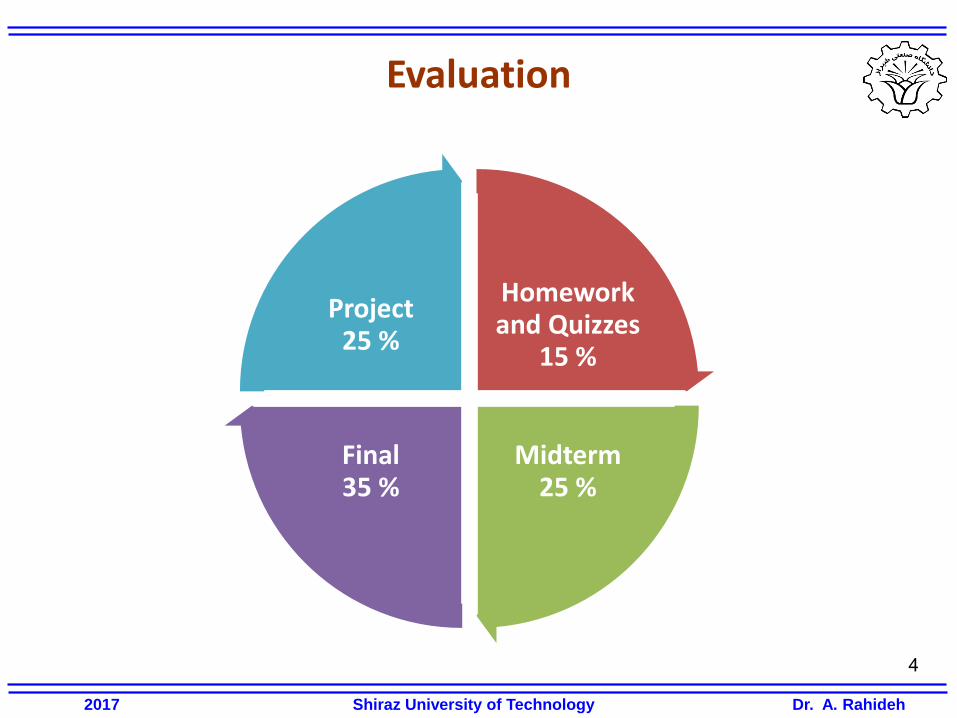
Evaluation
Homework and Quizzes
15 %
Midterm 25 %
Final 35 %
Project 25 %
2017 Shiraz University of Technology Dr. A. Rahideh
5
Table of Contents
2017 Shiraz University of Technology Dr. A. Rahideh
1. Introduction
2. Transformers
3. Reference-Frame Theory
4. Induction Machines
5. Synchronous Machines
6
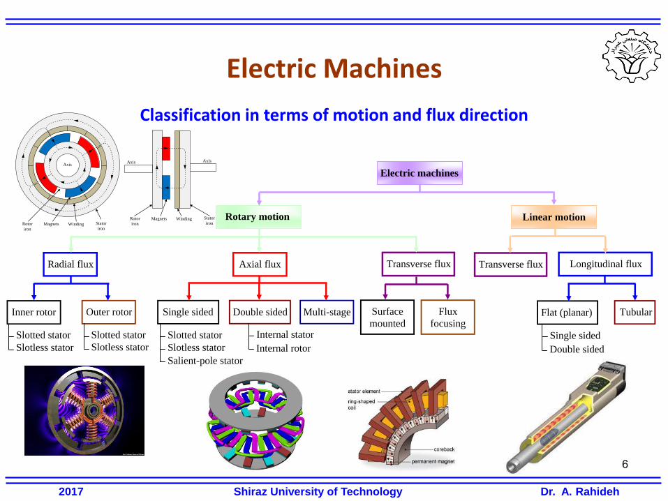
Electric Machines
Classification in terms of motion and flux direction
Radial flux Axial flux
Linear motion Rotary motion
Inner rotor Outer rotor Single sided Double sided Multi-stage
Slotless stator
Slotted stator Slotted stator
Electric machines
Slotless stator
Slotted stator
Salient-pole stator
Internal stator
Internal rotor Slotless stator
Transverse flux Longitudinal flux Transverse flux
Flat (planar) Tubular
Single sided
Double sided
Surface
mounted
Flux
focusing
Axis
Rotor
iron
Magnets Winding Stator
iron
Axis Axis
Rotor
iron Magnets Winding Stator
iron
2017 Shiraz University of Technology Dr. A. Rahideh
7
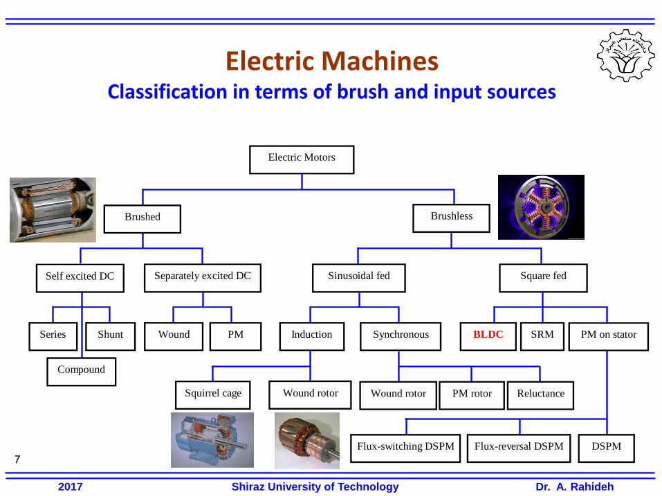
Electric Machines Classification in terms of brush and input sources
Electric Motors
Brushed Brushless
Self excited DC Separately excited DC
Series Shunt Wound PM
Sinusoidal fed Square fed
SRM BLDC Induction Synchronous
Squirrel cage Wound rotor Wound rotor PM rotor Reluctance
Compound
PM on stator
DSPM Flux-reversal DSPM Flux-switching DSPM
2017 Shiraz University of Technology Dr. A. Rahideh
8
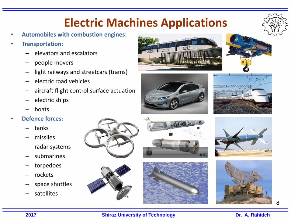
Electric Machines Applications • Automobiles with combustion engines:
• Transportation:
– elevators and escalators
– people movers
– light railways and streetcars (trams)
– electric road vehicles
– aircraft flight control surface actuation
– electric ships
– boats
• Defence forces:
– tanks
– missiles
– radar systems
– submarines
– torpedoes
– rockets
– space shuttles
– satellites
2017 Shiraz University of Technology Dr. A. Rahideh

• Medical and healthcare equipment:
– dentist’s drills
– electric wheelchairs
– air compressors
– rehabilitation equipment
– artificial heart motors
• Power tools:
– drills
– hammers
– screwdrivers
– grinders
– polishers
– saws
– sanders
– sheep shearing hand-pieces
• Renewable energy systems
• Research and exploration equipment 9
Electric Machines Applications
2017 Shiraz University of Technology Dr. A. Rahideh
10
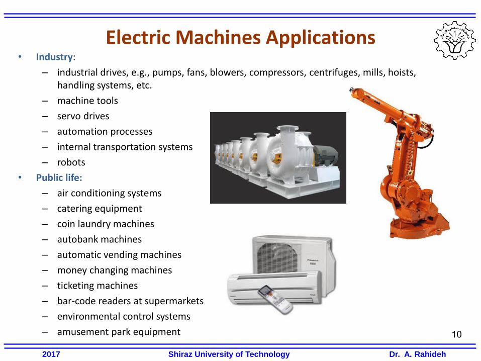
Electric Machines Applications • Industry:
– industrial drives, e.g., pumps, fans, blowers, compressors, centrifuges, mills, hoists, handling systems, etc.
– machine tools
– servo drives
– automation processes
– internal transportation systems
– robots
• Public life:
– air conditioning systems
– catering equipment
– coin laundry machines
– autobank machines
– automatic vending machines
– money changing machines
– ticketing machines
– bar-code readers at supermarkets
– environmental control systems
– amusement park equipment
2017 Shiraz University of Technology Dr. A. Rahideh
11
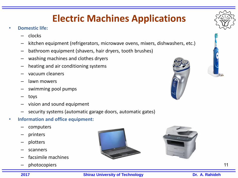
Electric Machines Applications • Domestic life:
– clocks
– kitchen equipment (refrigerators, microwave ovens, mixers, dishwashers, etc.)
– bathroom equipment (shavers, hair dryers, tooth brushes)
– washing machines and clothes dryers
– heating and air conditioning systems
– vacuum cleaners
– lawn mowers
– swimming pool pumps
– toys
– vision and sound equipment
– security systems (automatic garage doors, automatic gates)
• Information and office equipment:
– computers
– printers
– plotters
– scanners
– facsimile machines
– photocopiers
2017 Shiraz University of Technology Dr. A. Rahideh
12
Modelling & Simulation
• Model: a set of equations which represent the behaviour of a system.
• Modelling: the process to derive a set of governing equations which represent the behaviour of a system
• Simulation: the implementation of the derived equations to find the response of the system to a given input
2017 Shiraz University of Technology Dr. A. Rahideh
13
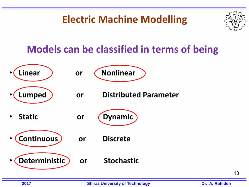
Electric Machine Modelling
Models can be classified in terms of being
• Linear or Nonlinear
• Lumped or Distributed Parameter
• Static or Dynamic
• Continuous or Discrete
• Deterministic or Stochastic
2017 Shiraz University of Technology Dr. A. Rahideh
14
Electric Machine Modelling
Linear vs. Nonlinear Models
• A model is linear if the superposition and homogeneity rules
are held;
• Otherwise, the model is nonlinear.
• A nonlinear model can be linearized around an operating point.
Both linear & nonlinear models are discussed.
2017 Shiraz University of Technology Dr. A. Rahideh
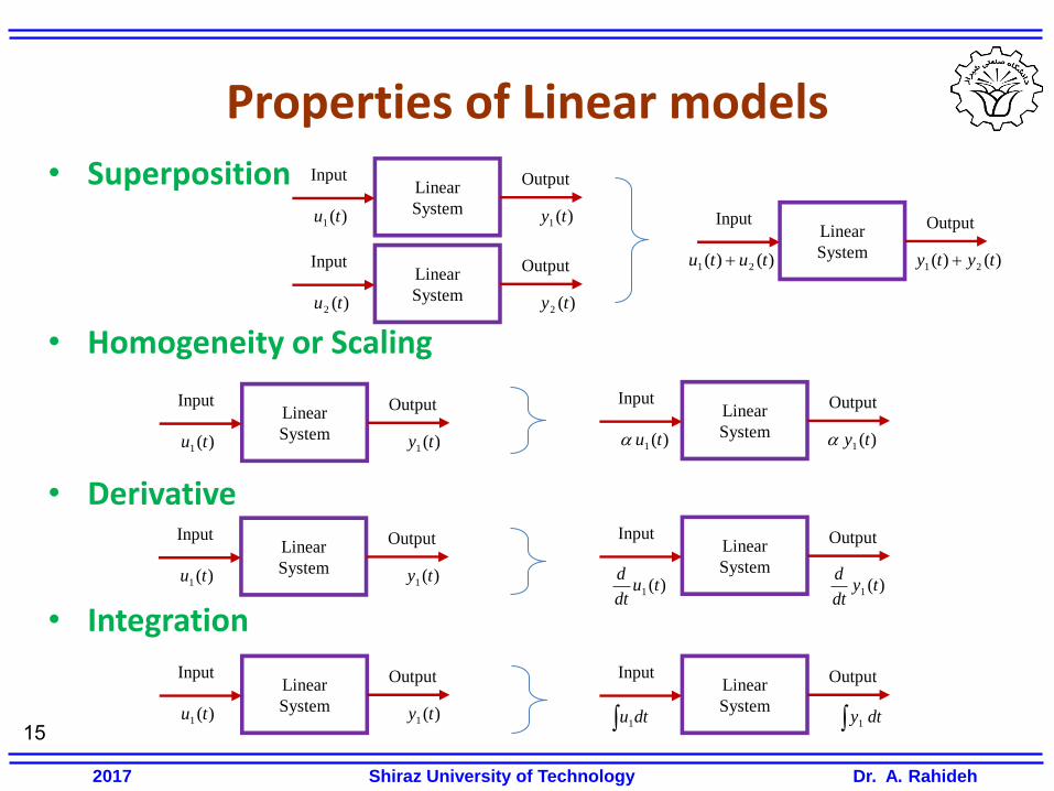
• Superposition
• Homogeneity or Scaling
• Derivative
• Integration
15
Properties of Linear models
Linear
System
Input Output
)(1 tu )(1 ty
Linear
System
Input Output
)(2 tu )(2 ty
Linear
System
Input Output
)()( 21 tutu )()( 21 tyty
Linear
System
Input Output
)(1 tu )(1 ty
Linear
System
Input Output
)(1 tu )(1 ty
Linear
System
Input Output
)(1 tu )(1 ty
Linear
System
Input Output
)(1 tudt
d )(1 tydt
d
Linear
System
Input Output
)(1 tu )(1 ty
Linear
System
Input Output
dtu 1 dty1
2017 Shiraz University of Technology Dr. A. Rahideh
16
Electric Machine Modelling
Lumped vs. Distributed Parameter Models
• Lumped parameter models are described by ordinary
differential equations with only one independent variable which is time.
• Distributed parameter models are described by partial differential equations with time and one or more spatial coordinates as independent variables.
We focus on lumped parameter models.
2017 Shiraz University of Technology Dr. A. Rahideh
17
Electric Machine Modelling
Static vs. Dynamic Models
• Static models do not take time variations into account.
• Static models are normally used for machine design purposes.
• Dynamic models take time-varying characteristics into account.
• Dynamic models are employed to dynamically analyse electric machines.
• Dynamic models are used for control design purposes.
We focus on dynamic models.
2017 Shiraz University of Technology Dr. A. Rahideh
18
Electric Machine Modelling
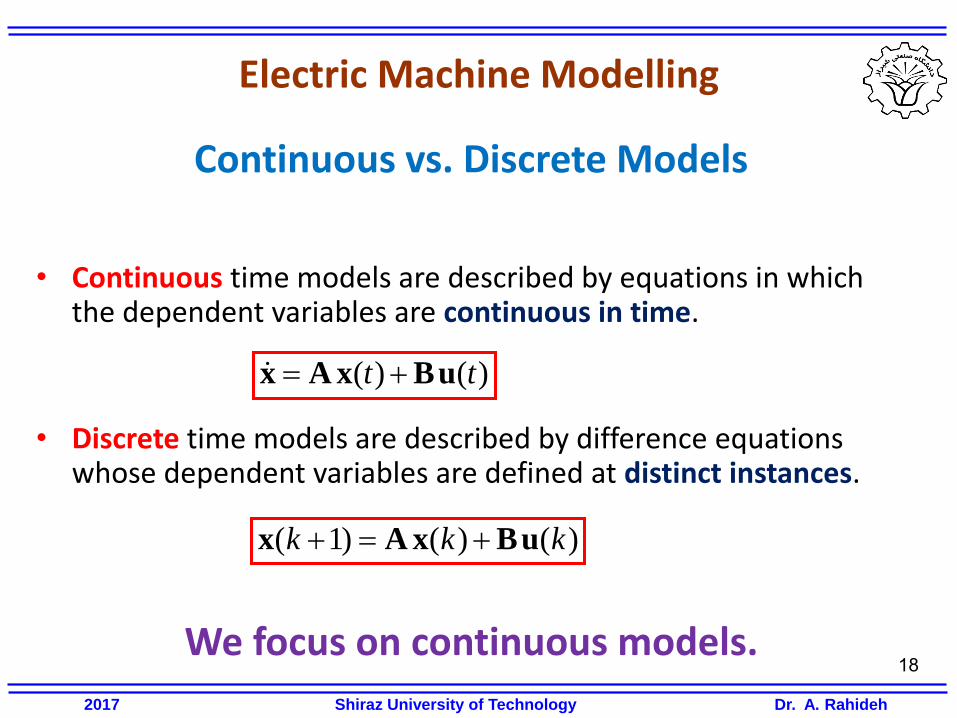
Continuous vs. Discrete Models
• Continuous time models are described by equations in which the dependent variables are continuous in time.
• Discrete time models are described by difference equations whose dependent variables are defined at distinct instances.
We focus on continuous models.
2017 Shiraz University of Technology Dr. A. Rahideh
)()( tt uBxAx
)()()1( kkk uBxAx
19
Electric Machine Modelling
Deterministic vs. Stochastic Models
• A model is deterministic if there are no chance factors.
• A model is stochastic if chance factors are taken into account.
We focus on deterministic models.
2017 Shiraz University of Technology Dr. A. Rahideh
20
Simplicity vs. Accuracy
• Increasing complexity of a model can improve the accuracy.
• There should be a compromise between the simplicity and accuracy of the model.
• Therefore it may be necessary to ignore some inherent physical property.
• The ignored properties should not have significant effect on the model response.
2017 Shiraz University of Technology Dr. A. Rahideh
21
Different ways of model representation
1. Time domain
• Differential equations (for both linear & nonlinear systems)
• State-space equations (for both linear & nonlinear systems)
• Impulse response (only for linear systems)
2. Frequency domain
• Transfer function (only for linear systems)
• Frequency response (only for linear systems)
2017 Shiraz University of Technology Dr. A. Rahideh
22
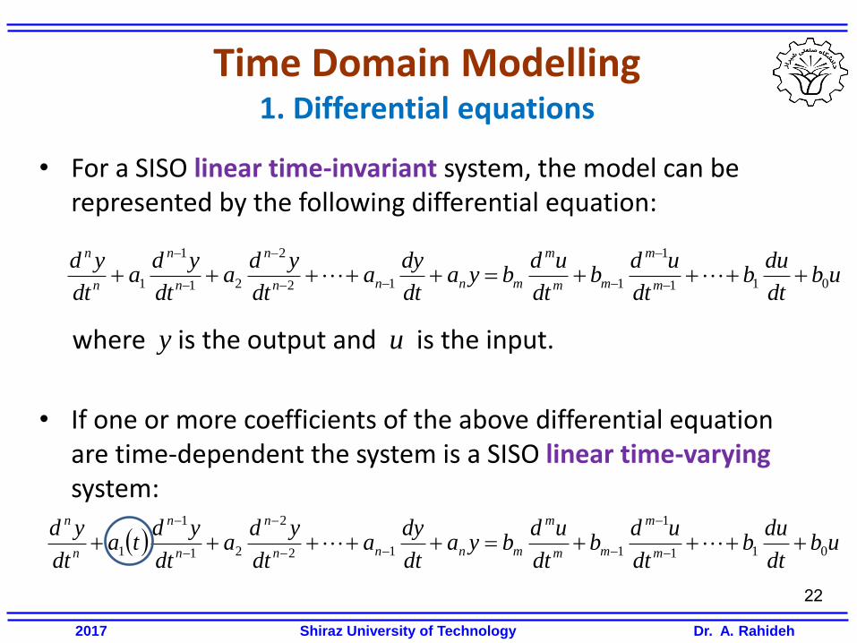
Time Domain Modelling 1. Differential equations
• For a SISO linear time-invariant system, the model can be represented by the following differential equation: where y is the output and u is the input.
• If one or more coefficients of the above differential equation
are time-dependent the system is a SISO linear time-varying system:
ubdt
dub
dt
udb
dt
udbya
dt
dya
dt
yda
dt
yda
dt
ydm
m
mm
m
mnnn
n
n
n
n
n
011
1
112
2
21
1
1
ubdt
dub
dt
udb
dt
udbya
dt
dya
dt
yda
dt
ydta
dt
ydm
m
mm
m
mnnn
n
n
n
n
n
011
1
112
2
21
1
1
2017 Shiraz University of Technology Dr. A. Rahideh
23
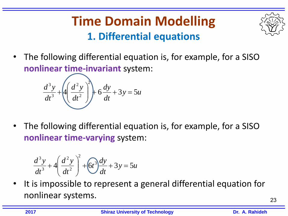
Time Domain Modelling 1. Differential equations
• The following differential equation is, for example, for a SISO nonlinear time-invariant system:
• The following differential equation is, for example, for a SISO nonlinear time-varying system:
• It is impossible to represent a general differential equation for nonlinear systems.
uydt
dy
dt
yd
dt
yd5364
2
2
2
3
3
uydt
dyt
dt
yd
dt
yd5364 3
2
2
2
3
3
2017 Shiraz University of Technology Dr. A. Rahideh

• State: The state of a dynamic system is the smallest set of variables (called state variables) such that the knowledge of these variables at t=t0, together with the knowledge of the input for , completely determines the behaviour of the system for any time .
• State vector: if n state variables are needed to completely describe the behaviour of a given system therefore:
24
Time Domain Modelling 2. State space equations
0tt
T
21 nxxx x
0tt
2017 Shiraz University of Technology Dr. A. Rahideh
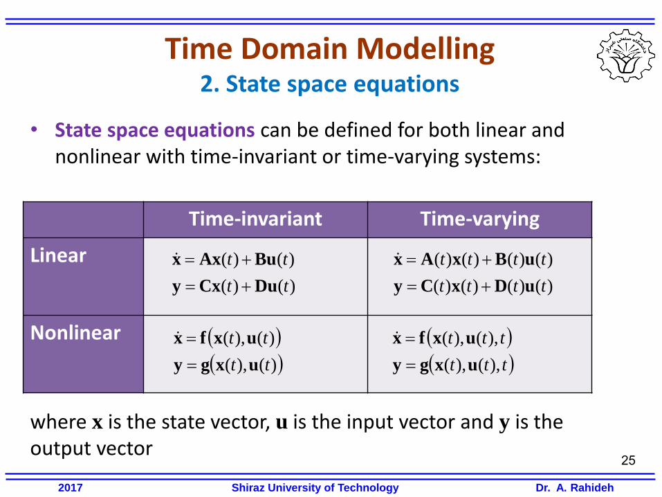
• State space equations can be defined for both linear and nonlinear with time-invariant or time-varying systems:
where x is the state vector, u is the input vector and y is the output vector
Time-invariant Time-varying
Linear
Nonlinear
25
Time Domain Modelling 2. State space equations
)()(
)()(
tt
tt
DuCxy
BuAxx
)()()()(
)()()()(
tttt
tttt
uDxCy
uBxAx
)(),(
)(),(
tt
tt
uxgy
uxfx
ttt
ttt
),(),(
),(),(
uxgy
uxfx
2017 Shiraz University of Technology Dr. A. Rahideh
26
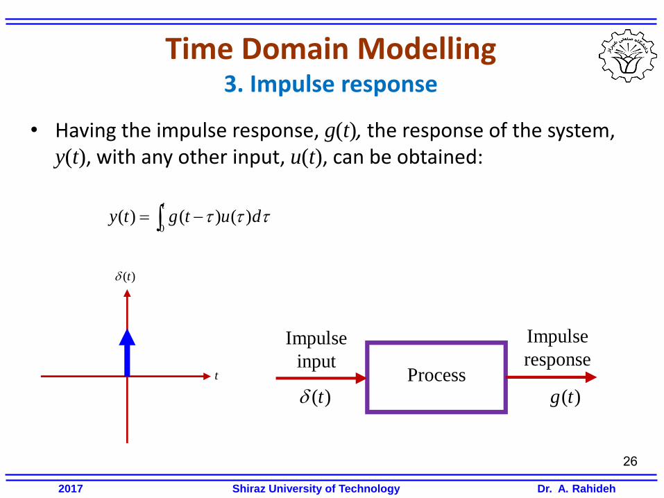
Time Domain Modelling 3. Impulse response
• Having the impulse response, g(t), the response of the system, y(t), with any other input, u(t), can be obtained:
t
dutgty0
)()()(
t
)(t
Process
Impulse
input
Impulse
response
)(t )(tg
2017 Shiraz University of Technology Dr. A. Rahideh
27
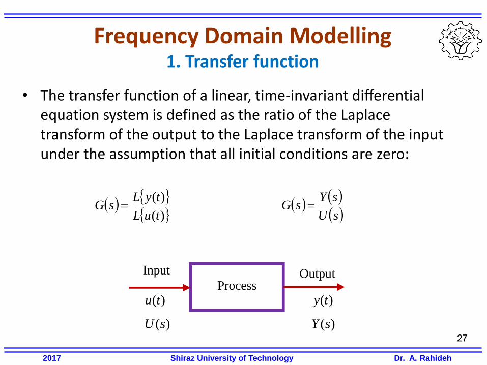
Frequency Domain Modelling 1. Transfer function
• The transfer function of a linear, time-invariant differential equation system is defined as the ratio of the Laplace transform of the output to the Laplace transform of the input under the assumption that all initial conditions are zero:
)(
)(
tuL
tyLsG
sU
sYsG
Process
Input Output
)(tu )(ty
)(sU )(sY
2017 Shiraz University of Technology Dr. A. Rahideh
28
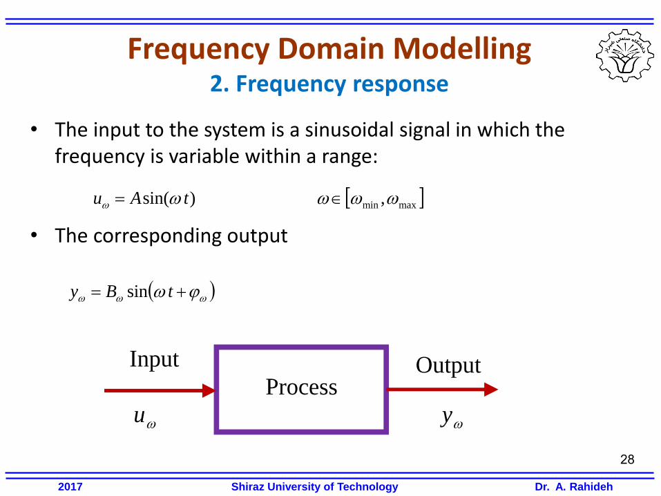
Frequency Domain Modelling 2. Frequency response
• The input to the system is a sinusoidal signal in which the frequency is variable within a range:
• The corresponding output
)sin( tAu
tBy sin
maxmin ,
Process
Input Output
u y
2017 Shiraz University of Technology Dr. A. Rahideh
29
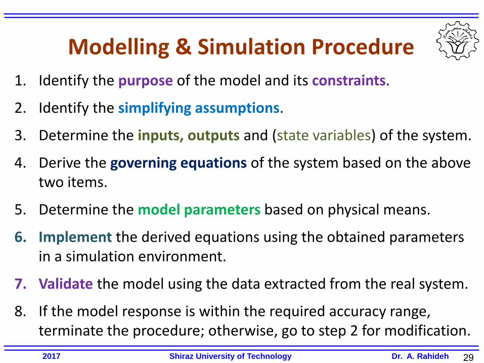
Modelling & Simulation Procedure
1. Identify the purpose of the model and its constraints.
2. Identify the simplifying assumptions.
3. Determine the inputs, outputs and (state variables) of the system.
4. Derive the governing equations of the system based on the above two items.
5. Determine the model parameters based on physical means.
6. Implement the derived equations using the obtained parameters in a simulation environment.
7. Validate the model using the data extracted from the real system.
8. If the model response is within the required accuracy range, terminate the procedure; otherwise, go to step 2 for modification.
2017 Shiraz University of Technology Dr. A. Rahideh

30
Modelling & Simulation Procedure
Example: Assume a separately excited DC motor is available and we need to derive a dynamic and continuous-time model of the system.
1. Identify the purpose of the model and its constraints.
• The purpose of the model is to design a control system.
• The model should be dynamic, continuous, deterministic and lumped parameter (constraint).
2. Identify the simplifying assumptions.
• The saturation effects are neglected.
• The core losses are neglected.
• Armature reaction is neglected. 2017 Shiraz University of Technology Dr. A. Rahideh
31
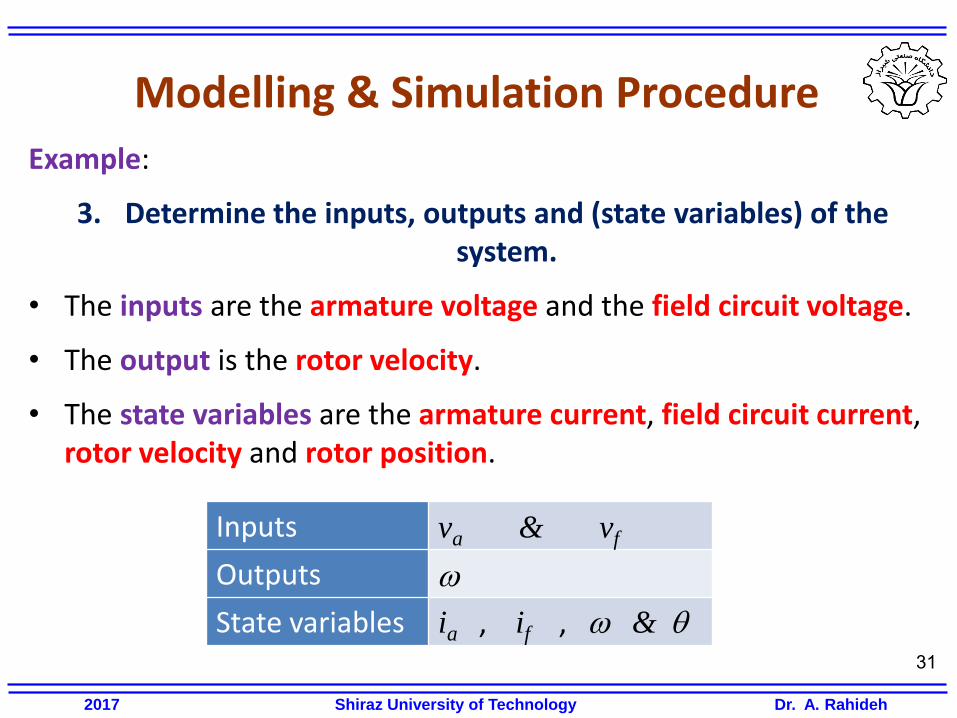
Modelling & Simulation Procedure
Example:
3. Determine the inputs, outputs and (state variables) of the system.
• The inputs are the armature voltage and the field circuit voltage.
• The output is the rotor velocity.
• The state variables are the armature current, field circuit current, rotor velocity and rotor position.
2017 Shiraz University of Technology Dr. A. Rahideh
Inputs va & vf
Outputs
State variables ia , if , & q
32
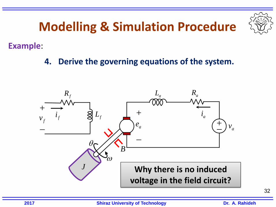
Modelling & Simulation Procedure
Example:
4. Derive the governing equations of the system.
2017 Shiraz University of Technology Dr. A. Rahideh
av ai
+ _
aR
+
ae
_
aL
J
q
B
fi fL
fR
fv +
_
Why there is no induced voltage in the field circuit?
33
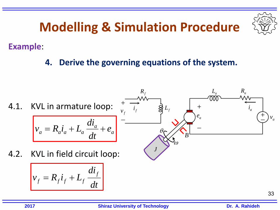
Modelling & Simulation Procedure
Example:
4. Derive the governing equations of the system.
4.1. KVL in armature loop:
4.2. KVL in field circuit loop:
2017 Shiraz University of Technology Dr. A. Rahideh
av ai
+ _
aR
+
ae
_
aL
J
q
B
fi fL
fR
fv +
_
aa
aaaa edt
diLiRv
dt
diLiRv
f
ffff
34
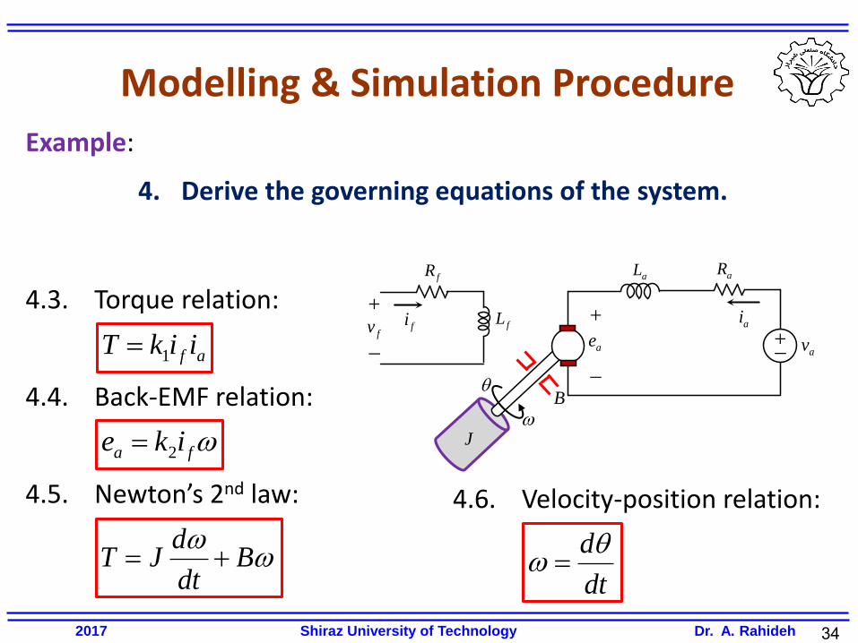
Modelling & Simulation Procedure
Example:
4. Derive the governing equations of the system.
4.3. Torque relation:
4.4. Back-EMF relation:
4.5. Newton’s 2nd law:
2017 Shiraz University of Technology Dr. A. Rahideh
av ai
+ _
aR
+
ae
_
aL
J
q
B
fi fL
fR
fv +
_ af iikT 1
fa ike 2
dt
dq
B
dt
dJT
4.6. Velocity-position relation:
35
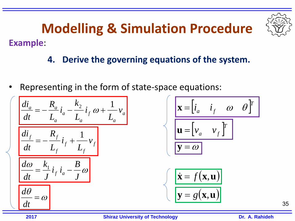
Modelling & Simulation Procedure Example:
4. Derive the governing equations of the system.
• Representing in the form of state-space equations:
2017 Shiraz University of Technology Dr. A. Rahideh
q
dt
d
J
Bii
J
k
dt
daf 1
a
a
f
a
a
a
aa vL
iL
ki
L
R
dt
di 12
f
f
f
f
ffv
Li
L
R
dt
di 1
Tfa ii qx
Tfa vvu
y
uxx ,f
uxy ,g
36
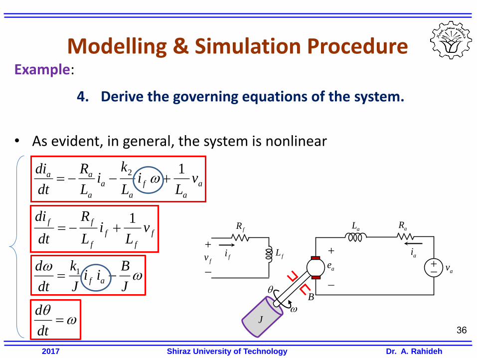
Modelling & Simulation Procedure Example:
4. Derive the governing equations of the system.
• As evident, in general, the system is nonlinear
2017 Shiraz University of Technology Dr. A. Rahideh
q
dt
d
J
Bii
J
k
dt
daf 1
a
a
f
a
a
a
aa vL
iL
ki
L
R
dt
di 12
f
f
f
f
ffv
Li
L
R
dt
di 1
av ai
+ _
aR
+
ae
_
aL
J
q
B
fi fL
fR
fv +
_
37
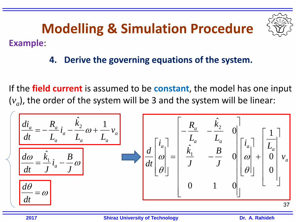
Modelling & Simulation Procedure Example:
4. Derive the governing equations of the system.
If the field current is assumed to be constant, the model has one input (va), the order of the system will be 3 and the system will be linear:
2017 Shiraz University of Technology Dr. A. Rahideh
q
dt
d
J
Bi
J
k
dt
da 1
ˆ
a
aa
a
a
aa vLL
ki
L
R
dt
di 1ˆ2
a
aa
aa
a
a
v
Li
J
B
J
k
L
k
L
R
i
dt
d
0
0
1
010
0ˆ
0ˆ
1
2
q
q
38
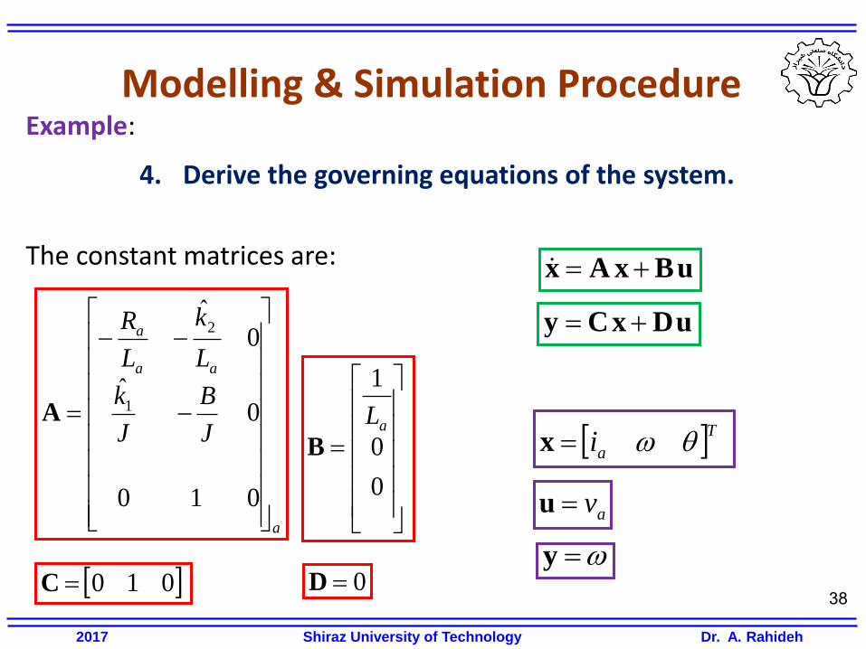
Modelling & Simulation Procedure Example:
4. Derive the governing equations of the system.
The constant matrices are:
2017 Shiraz University of Technology Dr. A. Rahideh
uBxAx
uDxCy
a
aa
a
J
B
J
k
L
k
L
R
010
0ˆ
0ˆ
1
2
A
0
0
1
aL
B
010C 0D
Tai qx
avu
y
39
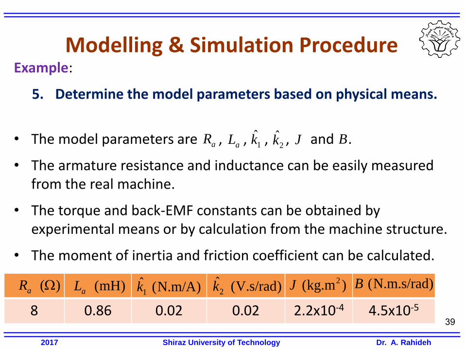
Modelling & Simulation Procedure Example:
5. Determine the model parameters based on physical means.
• The model parameters are , , , , and .
• The armature resistance and inductance can be easily measured from the real machine.
• The torque and back-EMF constants can be obtained by experimental means or by calculation from the machine structure.
• The moment of inertia and friction coefficient can be calculated.
2017 Shiraz University of Technology Dr. A. Rahideh
2k̂aRaL 1k̂ J B
8 0.86 0.02 0.02 2.2x10⁻⁴ 4.5x10⁻⁵
)(aR )mH(aL )N.m/A(ˆ1k )V.s/rad(ˆ
2k )kg.m( 2J )N.m.s/rad(B
40
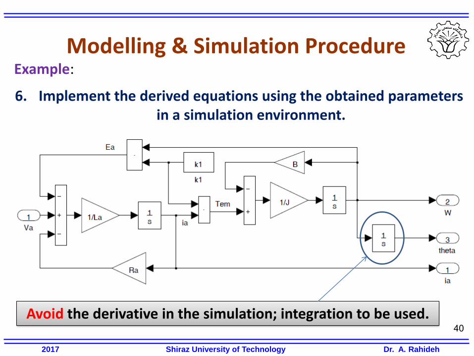
Modelling & Simulation Procedure Example:
6. Implement the derived equations using the obtained parameters in a simulation environment.
2017 Shiraz University of Technology Dr. A. Rahideh
Avoid the derivative in the simulation; integration to be used.