Homogenized boundary conditions and resonance effects

in Faraday cages

D. P. Hewett and I. J. Hewitt

Mathematical Institute, University of Oxford, UK

hewett@maths.ox.ac.uk, hewitt@maths.ox.ac.uk

April 28, 2017

Abstract

We present a mathematical study of two-dimensional electrostatic and electromagnetic shield-ing by a cage of conducting wires (the so-called ‘Faraday cage effect’). Taking the limit as thenumber of wires in the cage tends to infinity we use the asymptotic method of multiple scalesto derive continuum models for the shielding, involving homogenized boundary conditions onan effective cage boundary. We show how the resulting models depend on key cage parameterssuch as the size and shape of the wires, and, in the electromagnetic case, on the frequency andpolarisation of the incident field. In the electromagnetic case there are resonance effects, wherebyat frequencies close to the natural frequencies of the equivalent solid shell, the presence of thecage actually amplifies the incident field, rather than shielding it. By appropriately modifyingthe continuum model we calculate the modified resonant frequencies, and their associated peakamplitudes. We discuss applications to radiation containment in microwave ovens and acousticscattering by perforated shells.

1 Introduction

The Faraday cage effect is the phenomenon whereby electric fields and electromagnetic waves canbe blocked by a wire mesh. The effect was demonstrated experimentally by Faraday in 1836 [13],was familiar to Maxwell [17], and its practical application in isolating electrical systems and circuitsis well known to modern-day engineers and physicists alike. However, somewhat surprisingly theredoes not seem to be a widely-known mathematical analysis quantifying the effectiveness of theshielding as a function of the basic cage properties (e.g. the geometry of the cage, and the thickness,shape and spacing of the wires in the mesh from which it is constructed). The recent publication[4] provided such an analysis for the two-dimensional electrostatic problem where the cage is a ringof M equally spaced circular wires of small radius r 1/M held at a common constant potential,which can be formulated as a Dirichlet problem for the Laplace equation. It was found in [4] thatthe shielding effect of such a Faraday cage is surprisingly weak: as the number of wires M tends toinfinity the magnitude of the field inside the cage in general decays at best only inverse linearly inM , rather than exponentially, as one might infer from certain treatments of the Faraday cage effectin the physics literature (see e.g [14, Sec. 7-5]).

One of the key tools used in [4] to study the Faraday cage effect in the regime of large M wasa continuum model in which the shielding effect of the discrete wires is replaced by a homogenizedboundary condition on an infinitesimally thin interface between the “inside” and “outside” of thecage. Such boundary conditions can be derived by matching asymptotic expansions of the fieldaway from the mesh with expansions in a boundary layer close to the mesh, where a multiple

1

arX

iv:1

601.

0694

4v3

[m

ath-

ph]

27

Apr

201

7

scales approximation can be applied (cf. [4, §5 and Appendix C], and the closely related work in[9, 10, 11, 3]).

The current paper extends the analysis of [4] in a number of significant ways. Firstly, we explainhow the homogenized boundary condition of [4] generalises to arbitrary wire shapes (not necessarilycircular). Secondly, we investigate the ‘thick wire’ regime in which r = O (1/M) (the model proposedin [4] is valid only for r 1/M and is in general ill-posed for r = O (1/M).) Thirdly, we considerthe analogous Neumann problem, where the interesting regime is not that of small wires, but rathersmall gaps between wires. Finally, and perhaps most significantly, we undertake a detailed studyof the two-dimensional electromagnetic problem in which an external time-harmonic wave field (asolution of the Helmholtz equation) is incident on the cage. We show that, under appropriateassumptions on the wavelength and the wire radii, the leading order wave field satisfies the samehomogenized boundary conditions as in the Laplace case. However, in the wave problem there isthe possibility of resonance, where the presence of the cage actually amplifies the incident field,rather than shielding it. For the Dirichlet problem, such resonance effects are strongest in the ‘thickwire’ regime in which r = O (1/M), and when the wavelength is close to (but not in general equalto) a resonant wavelength of the idealised cage in which the wire mesh is replaced by a solid shell.We show how to modify the continuum model to deal with such resonances, and use our modifiedmodel to calculate precisely the wavelength at which the maximum amplification is observed, andthe associated peak amplitude, validating our predictions against numerical simulations.

We end this introduction with some comments on related literature. Firstly, we acknowledgethat there is already a substantial literature concerning the rigorous analysis of homogenizationprocedures for potential and scattering problems involving thin, rapidly-varying interfaces. Whilewe do not attempt a comprehensive review, we note in particular the works [5, 6, 10, 11, 9, 21,22, 18, 19, 12], which consider problems closely related (but different) to those studied here. Manyof these studies adopt a similar multiple-scales-based approach to ours, albeit from a slightly morerigorous point of view, and some (e.g. [6]) derive higher order asymptotic approximations thanthose considered here. What sets our work apart from this literature is that we are concernedless with formulating high order approximations and proving rigorous error estimates and morewith understanding the qualitative and quantitative behaviour of the leading order homogenizedapproximations - in particular their shielding performance - something which to date does notappear to have been studied systematically. Secondly, we mention [15], which treats the Dirichletproblem for a circular cage of small equally-spaced wires using the so-called “Foldy method” frommultiple scattering theory, in which the wires act as point sources and the geometrical assumptionspermit a semi-analytical solution for the associated amplitudes in terms of the discrete Fouriertransform. This method appears to be closely related to the lowest order version of the Mikhlin-type numerical method used in [4], higher order versions of which shall be our main source ofnumerical approximations for the circular wire case. The analysis of [15] does not cover the regimer = O (1/M) and does not treat resonance effects.

2 Problem formulation

Let Ω− be a bounded simply connected open subset of the plane with smooth boundary Γ = ∂Ω− andlet Ω+ := R2 \ Ω− denote the complementary exterior domain. For convenience we will routinelyidentify the (x, y)-plane with the complex z-plane, z = x + iy. We consider a ‘cage’ of M non-intersecting wires KjMj=1 (compact subsets of the plane, defined in more detail shortly) centred at

points zjMj=1 along Γ with constant separation (measured with respect to arc length along Γ)

ε = |Γ|/M,

2

ΓΩ−

Ω+

(x, y)

ns

K1

K2Kj

KM

ε

(a)

KKε

N

S

S = 1/2

S = −1/2

δ

(b)

ξ

η

K

1

(c)

Figure 1: (a) Faraday cage geometry and the outer coordinates (x, y) and (n, s), with the curveΓ on which the wires are centred shown as a dashed line. The dotted lines either side of the wireKj are curves of constant s = sj ± ε/2, corresponding to the lines S = ±1/2 in the boundarylayer coordinates. (b) The cell problem geometry and the boundary layer coordinates (N,S) =(n/ε, s/ε), showing the scaled wire shape K (solid boundary; Model 2) and the perturbation Kε(dashed boundary; Model 1). (c) The reference wire shape K and the inner inner coordinates (ξ, η).

where |Γ| is the total length of Γ; for an illustration see Figure 1(a). We set D := R2 \(⋃M

j=1Kj

).

The electrostatic problem is formulated as follows. Given a compactly supported source functionf , we seek a real-valued potential φ(z) satisfying

∇2φ = f in D, (1)

φ = 0 on ∂Kj , j = 1, . . . ,M, (2)

φ(z) ∼(

1

2π

∫Df

)log(|z|) +O (1) as z →∞. (3)

Condition (2) models the fact that the wires are electrically connected, e.g. at infinity in the thirddimension. Condition (3) ensures that the cage possesses zero net charge. We note that the for-mulation (1)-(3) is different (but equivalent) to that in [4], where the constant term at infinity in(3) was zero, with φ taking an unknown (and in general non-zero) constant value on the wires. Forcompleteness we also consider the Neumann problem in which (2) is replaced by

∂φ

∂ν= 0 on ∂Kj , j = 1, . . . ,M, (4)

where ν denotes a unit normal vector on ∂Kj , and O (1) is replaced by o(1) in (3). While not havingany obvious electrostatic application, this could represent a model for inviscid incompressible fluidflow due to a source in the presence of a cage of impermeable wires.

The time-harmonic electromagnetic problem can be formulated in terms of two complex-valuedscalar fields, representing the out-of-plane components of the electric and magnetic fields respectively,both of which satisfy the Helmholtz equation

(∇2 + k2)φ = f in D, (5)

for appropriate source functions f , where k > 0 is the (nondimensional) wavenumber. The out-of-plane component of the electric field (TE mode) satisfies the Dirichlet boundary condition (2)and the out-of-plane component of the magnetic field (TM mode) satisfies the Neumann boundarycondition (4). At infinity both fields are assumed to satisfy an outgoing radiation condition. These

3

two problems also model the analogous acoustic scattering problems with sound-soft and sound-hardboundary conditions respectively.

The goal of this paper is to determine the leading order asymptotic solution behaviour of theabove problems as the number of wires M tends to infinity, equivalently, as the wire separation εtends to zero1. To make this goal well-defined we need to specify how the wire size, shape andorientation should vary as ε → 0. In particular, in order that the wires remain disjoint as ε → 0(so that the wires form a ‘cage’ and not a solid shell), the wire radii must in general decrease inproportion to ε (or faster).

We consider two different models, defining a reference wire shape either in local Cartesian co-ordinates aligned with Γ, or in local curvilinear coordinates that conform to Γ. Since Γ is smooththere is no difference between these models at leading order, but the distinction affects higher or-der corrections (due to the curvature of Γ) that will enter some of our calculations. To make thedefinitions specific, we must introduce some further notation.

Close to Γ we can change from Cartesian coordinates (x, y) to orthogonal curvilinear coordi-nates (n, s), such that n is the distance from (x, y) to the closest point on Γ (positive/negative nrepresenting points inside Ω+ and Ω− respectively), and s is arc length along Γ to this closest pointmeasured counterclockwise from some reference point on Γ. Given a reference point zj on Γ withcurvilinear coordinates (0, sj), we define local curvilinear coordinates (n, s) by n = n, s = s − sj ,and local Cartesian coordinates (x, y) such that the positive x axis is aligned to the positive n axisat zj . Explicitly, x+ iy = e−iθj (z − zj), where θj is the counter-clockwise angle from the positive xaxis to the outward normal vector to Γ at zj . To convert between these coordinate systems thereexists a diffeomorphism Fj : (−nj , nj) × (−ε/2, ε/2) → Uj , where Uj is an open neighbourhood ofzj and nj > 0 is a constant, such that (x, y) = Fj(n, s) (see Appendix A).

We are now ready to specify the wire geometries and their dependence on ε. For both models,we assume a fixed reference wire shape K; a compact subset of the plane for which the smallestclosed disc containing K has radius one and is centred at the origin (see Figure 1(c)).

In Model 1 we define a wire Kj of radius r > 0 centred at zj by the formula Kj = rK in the(x, y) coordinate system, which in the original z coordinates gives

Kj = zj + eiθj (rK). (6)

In Model 2 we use the same formula Kj = rK but interpreted in the (n, s) coordinate system, whichin the original z coordinates gives

Kj = zj + eiθjFj(rK). (7)

Examples are illustrated in Figure 2. The rationale for considering both wire models is thatModel 1 is the more natural from a physical point of view as the wire shape is independent of rin the original Cartesian coordinate system, while Model 2 is simpler from a mathematical pointof view as the wire shape is independent of r in the curvilinear coordinates in which we derive ourhomogenized boundary conditions (see §3). In many aspects of our analysis the two models producethe same results. But for some problems requiring higher-order boundary layer expansions theymay produce different results.

In order that the wires remain disjoint as ε→ 0 we assume that the wire radius r satisfies

r = δε,

1We assume that lengths have been nondimensionalised relative to a suitable macro-lengthscale (e.g. the radius ofthe smallest circle containing Γ) so that ε is a nondimensional parameter.

4

Γ Ω−

Ω+

ε

(a)

Γ Ω−

Ω+

ε

(b)

Γ Ω−

Ω+

ε

(c)

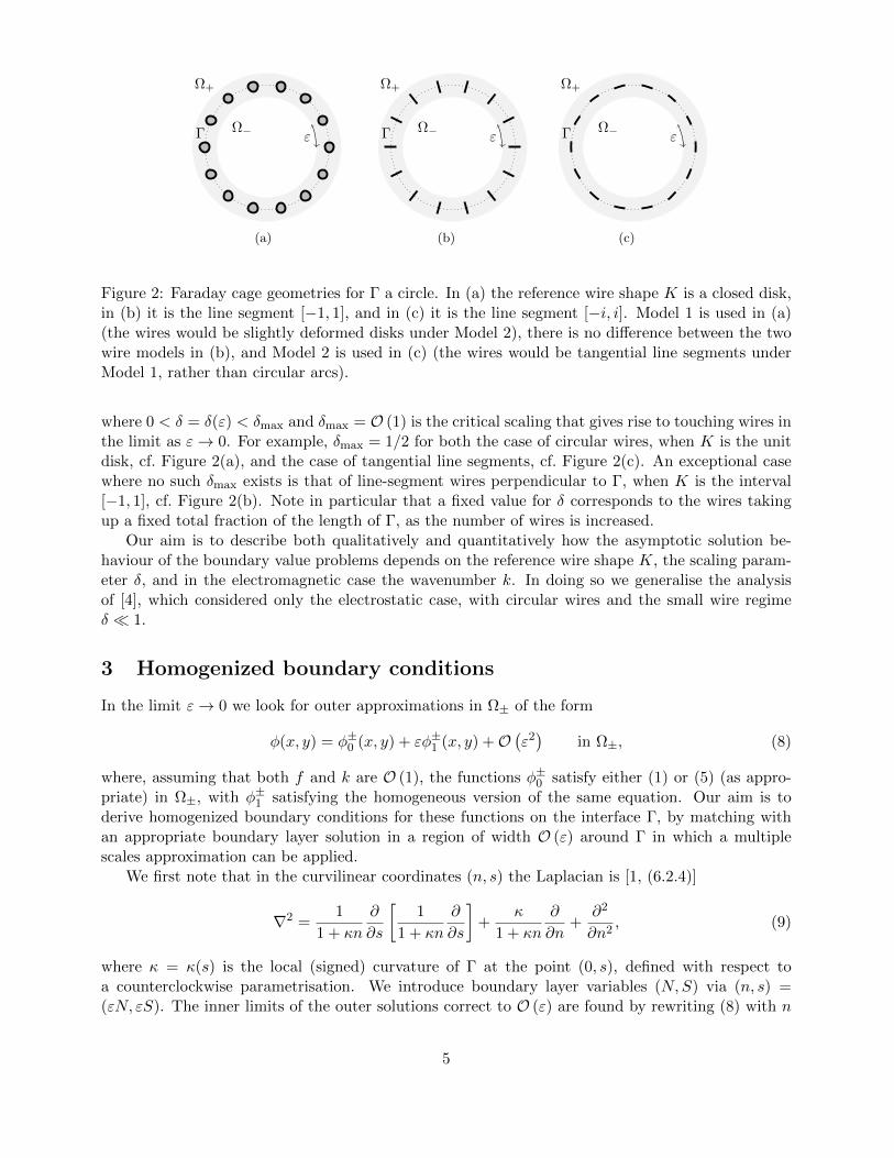
Figure 2: Faraday cage geometries for Γ a circle. In (a) the reference wire shape K is a closed disk,in (b) it is the line segment [−1, 1], and in (c) it is the line segment [−i, i]. Model 1 is used in (a)(the wires would be slightly deformed disks under Model 2), there is no difference between the twowire models in (b), and Model 2 is used in (c) (the wires would be tangential line segments underModel 1, rather than circular arcs).

where 0 < δ = δ(ε) < δmax and δmax = O (1) is the critical scaling that gives rise to touching wires inthe limit as ε→ 0. For example, δmax = 1/2 for both the case of circular wires, when K is the unitdisk, cf. Figure 2(a), and the case of tangential line segments, cf. Figure 2(c). An exceptional casewhere no such δmax exists is that of line-segment wires perpendicular to Γ, when K is the interval[−1, 1], cf. Figure 2(b). Note in particular that a fixed value for δ corresponds to the wires takingup a fixed total fraction of the length of Γ, as the number of wires is increased.

Our aim is to describe both qualitatively and quantitatively how the asymptotic solution be-haviour of the boundary value problems depends on the reference wire shape K, the scaling param-eter δ, and in the electromagnetic case the wavenumber k. In doing so we generalise the analysisof [4], which considered only the electrostatic case, with circular wires and the small wire regimeδ 1.

3 Homogenized boundary conditions

In the limit ε→ 0 we look for outer approximations in Ω± of the form

φ(x, y) = φ±0 (x, y) + εφ±1 (x, y) +O(ε2)

in Ω±, (8)

where, assuming that both f and k are O (1), the functions φ±0 satisfy either (1) or (5) (as appro-priate) in Ω±, with φ±1 satisfying the homogeneous version of the same equation. Our aim is toderive homogenized boundary conditions for these functions on the interface Γ, by matching withan appropriate boundary layer solution in a region of width O (ε) around Γ in which a multiplescales approximation can be applied.

We first note that in the curvilinear coordinates (n, s) the Laplacian is [1, (6.2.4)]

∇2 =1

1 + κn

∂

∂s

[1

1 + κn

∂

∂s

]+

κ

1 + κn

∂

∂n+

∂2

∂n2, (9)

where κ = κ(s) is the local (signed) curvature of Γ at the point (0, s), defined with respect toa counterclockwise parametrisation. We introduce boundary layer variables (N,S) via (n, s) =(εN, εS). The inner limits of the outer solutions correct to O (ε) are found by rewriting (8) with n

5

replaced by εN and re-expanding, giving

φ±0 (0, s) + ε

(N∂φ±0∂n

(0, s) + φ±1 (0, s)

)+O

(ε2), (10)

with the + and − signs for the cases N > 0 and N < 0 respectively.In the boundary layer we look for a solution in multiple-scales form

φ(n, s) = Φ(N,S; s), (11)

where Φ(N,S; s) is assumed to be 1-periodic in the fast tangential variable S. To determine theequation satisfied by Φ(N,S; s) we replace ∂/∂n by ε−1∂/∂N and ∂/∂s by ε−1∂/∂S + ∂/∂s in (9)and expand. The leading order result, for both the electrostatic and the wave problems (assumingk = O (1)), and for both wire Models 1 and 2, is

∂2Φ

∂N2+∂2Φ

∂S2+O (ε) = 0 in B, (12)

where B = (N,S) : |S| < 1/2 \ K, and K = δK (see Figure 1(b)). Periodicity requires

Φ(N,−1/2; s) = Φ(N, 1/2; s), (13)

and the conditions on ∂K are homogenous Dirichlet or Neumann conditions, as appropriate. Thesolution is required to match with the outer solution in (10) as N → ±∞.

A more detailed derivation of this boundary-layer problem is given in Appendix A, where wealso continue the expansion to O (ε). The analysis of the O (ε) terms is more involved for Model 1than for Model 2, because we have to account for the curvature of Γ and its distorting effect on thewire shape in the (N,S) coordinates (shown by Kε in Figure 1(b)). This distortion can be neglectedin the leading order problem above (and does not arise in Model 2); consequently, we leave theseawkward details to the appendix.

3.1 Dirichlet boundary conditions

In the case of Dirichlet boundary conditions the leading order behaviour of the boundary layersolution Φ(N,S; s) with linear behaviour as N → ±∞ (required for matching) can be written as

Φ(N,S; s) = ε(A+(s)Φ+(N,S) +A−(s)Φ−(N,S)

)+O

(ε2), (14)

where the functions Φ±(N,S) satisfy the following canonical cell problems (cf. Figure 1(b)):

∂2Φ±

∂N2+∂2Φ±

∂S2= 0 in B, (15)

Φ±(N,−1/2) = Φ±(N, 1/2), (16)

Φ± = 0 on ∂K, (17)

Φ+(N,S) ∼N + σ+, N →∞,τ+, N → −∞,

Φ−(N,S) ∼τ−, N →∞,−N + σ−, N → −∞.

(18)

For any given reference wire shape K and scaled radius δ one must solve (15)-(18), eitheranalytically or numerically, to determine the far-field constants σ± and τ±; some specific examplesare studied in Appendix B. We note that if K is symmetric in ξ then

Φ−(N,S) = Φ+(−N,S), σ+ = σ−, τ+ = τ−. (19)

6

Furthermore, we note that if δ 1 the scaled wire K effectively acts as a point sink in the celldomain, and a generalisation of the argument in [4, §C] proves that, outside an O (δ) neighbourhoodof K,

Φ+(N,S) ∼ 1

2π<πZ + log (2 sinhπZ) + log

1

2πδ+ a0

, Z = N + iS, (20)

where the K-dependent constant a0 satisfies a0 = lim%→∞(ψ− log %), where ψ is the unique solutionof Laplace’s equation in R2 \ K such that ψ = 0 on ∂K and ψ ∼ log % + O (1) as % → ∞, where% =

√ξ2 + η2. This constant is related to the logarithmic capacity of K, c(K), by a0 = − log c(K)

[20]. For K the unit disc, a0 = 0; for K a line segment of length 2, a0 = log 2 (for details seeAppendix B). From (20) it follows that

σ±, τ± ∼1

2π

(log

1

2πδ+ a0

)+O (δ) , δ → 0. (21)

Having extracted the far-field constants σ±, τ± from the solutions of (15)-(18), matching thelinear behaviour of (14) with that of (10) gives

A+(s) =∂φ+

0

∂n(0, s), A−(s) = −∂φ

−0

∂n(0, s), (22)

and matching constant terms then requires

εσ+∂φ+

0

∂n− ετ−

∂φ−0∂n

= φ+0 + εφ+

1 on Γ, (23)

ετ+∂φ+

0

∂n− εσ−

∂φ−0∂n

= φ−0 + εφ−1 on Γ. (24)

To proceed further we must consider the magnitude of the parameters σ±, τ±, which depend on thesize of δ (see Figure 9 for example). There are essentially three different regimes to consider.

Thick wires (δ = O (1)). If δ is strictly O (1) then σ±, τ± are O (1). Hence, at O (1) in (23)and (24),

φ+0 = φ−0 = 0 on Γ, (25)

so the leading order solution is that for a perfectly reflecting (Dirichlet) boundary at Γ. At O (ε),

φ+1 = σ+

∂φ+0

∂n− τ−

∂φ−0∂n

on Γ, (26)

φ−1 = τ+∂φ+

0

∂n− σ−

∂φ−0∂n

on Γ. (27)

Thin wires (δ 1). If δ 1 then σ±, τ± 1 (cf. (21)). In particular, there is a distinguishedscaling in which σ±, τ± = O (1/ε), which requires δ to be exponentially small with respect to 1/ε, i.e.δ = O

(e−c/ε

)for some c > 0. (This is essentially the same scaling as that considered in [21, 22, 5]

in a related context.) Suppose that we are in this regime, with σ±, τ± ∼ a1/ε+ a0 for some a1, a0.(E.g. if δ ∼ Ae−c/ε then a1 = c/(2π) and a0 = (log(1/(2πA))+a0)/(2π).) Then at O (1) in (23)-(24)we find that φ0 is continuous across Γ (i.e., φ+

0 = φ−0 ) and satisfies[∂φ0

∂n

]= αφ0 on Γ, (28)

7

where [∂φ0/∂n] = ∂φ+0 /∂n − ∂φ−0 /∂n and α = 1/a1. Higher order matching not detailed here

(requiring higher order expansion of the boundary layer problem as in Appendix A) reveals that thetwo-term approximation φ0 + εφ1 is also continuous across Γ and satisfies a similar condition,[

∂φ0

∂n+ ε

∂φ1

∂n

]= α (φ0 + εφ1) on Γ, (29)

where α = 1/(a1 + εa0). Recalling (21), we can express α in terms of δ as

α =2π

ε (log 1/(2πδ) + a0), (30)

which, in the special case of circular wires (for which a0 = 0) agrees with the effective boundarycondition derived in [4, §C]. Note that (29) is valid for the two-term approximation φ0 + εφ1; hencein this distinguished scaling the boundary condition derived in [4, §C] gives the solution correct toO (ε), not just to O (1). This explains the excellent agreement observed in [4] between numericalsolutions of the electrostatic problem and solutions of the outer problem subject to (29), even whenδ is not particularly small. We also note, however, that as δ increases, there may (depending on thevalue of a0) come a point at which α blows up to infinity; precisely, this occurs at the critical valueδ∞ = e−a0/(2π) (for circular wires δ∞ = 1/(2π) ≈ 0.16 < δmax = 1/2). For δ > δ∞, α is negativeand the resulting outer problem may be ill-posed (see later). But of course for such large values ofδ we are outside of this ‘thin-wire’ regime and the conditions (25)–(27) should be used instead of(29).

Very thin wires (δ O(e−c/ε

)). If δ O

(e−c/ε

)for every c > 0, then σ±, τ± 1/ε and

α 1, so that the leading order outer solution φ0 is just the free field solution of (1) or (5), i.e.that which would exist without the presence of the cage, and there is no shielding.

3.2 Neumann boundary condition

In the case of Neumann boundary conditions the requirement of linearity as N → ±∞ means thatthe leading order boundary layer solution can be expressed as

Φ(N,S; s) = A0(s) + ε(A1(s) +B1(s)Ψ(N,S)

)+O

(ε2), (31)

where Ψ(N,S) satisfies the canonical cell problem

∂2Ψ

∂N2+∂2Ψ

∂S2= 0 in B, (32)

Ψ(N,−1/2) = Ψ(N, 1/2), on S = ±1/2, (33)

∂Ψ

∂ν= 0 on ∂K, (34)

Ψ(N,S) ∼ N ± λ, N → ±∞, (35)

in which the constant λ is determined as part of the solution. This problem also appears elsewherein acoustics and fluid flow; it is sometimes referred to as a ‘blockage problem’, and the constant λas a ‘blockage coefficient’ [25, 7, 8]. Example solutions for Ψ(N,S) and λ are given in Appendix B.

Matching linear terms between (10) and (31) gives that

B1(s) =∂φ+

0

∂n=∂φ−0∂n

on Γ, (36)

8

so the gradient of the outer problem is continuous across Γ. Matching constant terms then gives

A0(s) + εA1(s)± λε∂φ0

∂n= φ±0 + εφ±1 on Γ. (37)

As in the Dirichlet case, to interpret (37) we must consider the magnitude of λ, which dependson both K and δ. The interesting limit in which λ is large is now not δ → 0, but rather δ → δmax,where δmax is the critical value of δ for which ∂K touches the cell walls S = ±1/2. (Recall thatδmax = 1/2 for K a disk.) When δmax − δ 1 we have λ 1. We consider separately the casesλ = O (1), λ = O (1/ε), and λ 1/ε.

Large gaps (δmax − δ = O (1)). In this case λ = O (1), and (37) implies that

A0(s) = φ+0 = φ−0 on Γ, (38)

so that, recalling (36), both φ0 and its normal derivative are continuous across Γ. Hence the leadingorder outer solution is just the free field solution of (1) or (5), and there is no shielding.

Small gaps (δmax − δ 1). In this case λ 1. We first consider the case λ = O (1/ε) andsuppose λ ∼ b1/ε + b0. For the case of circular wires, this would occur if 1

2 − δ = O(ε2); for line

segments it would require 12−δ = O

(e−c/ε

)for some c > 0 (see Appendix B). Matching the constant

terms then gives

A0(s)± b1B1(s) = φ±0 on Γ, (39)

which together with (36), and defining β = 2b1 and [φ0] = φ+0 − φ−0 , implies

[φ0

]= β

∂φ0

∂non Γ. (40)

For completeness we quote the higher order matching conditions, obtained using the results inAppendix A, [

∂φ1

∂n

]= 2κ(µ− µ)

∂φ0

∂n+ 2µ

∂2φ0

∂n∂s− 2µ

∂2φ0

∂n2on Γ, (41)

[φ1

]= 2b0

∂φ0

∂n+ b1

(∂φ+

1

∂n+∂φ−1∂n

)on Γ, (42)

where µ, µ and µ are constants determined from the higher order boundary-layer solutions. Thesedepend on the precise shape of the wires.

Rather than embarking on a detailed study of different cases, we concentrate on the case thatis perhaps of most interest for this small-gap situation; namely, when the wires form a perforatedshell around Γ (cf. Figure 2(c)). This corresponds to tangential line segments (i.e. K = [−i, i]) underModel 2, for which we find µ = µ = µ = 0, and λ ∼ −(1/π)(log π(1/2− δ)) (Appendix B). In thiscase (41) and (42) combine with (40) to give

[φ0 + εφ1

]= β

(∂φ0

∂n+ ε

∂φ1

∂n

)on Γ, (43)

where β = 2(b1 + εb0). If δ = 1/2 − Ae−c/ε then β = 2c/π − 2ε log(πA)/π. There is a dualitybetween (43) and condition (29) that holds in the Dirichlet case, although we note that for moregeneral wire shapes (43) may become more complicated.

9

Very small gaps (δmax − δ 1). In the case that λ O (1/ε), matching constant terms in(37) simply indicates that B1(s) = 0. Thus (36) gives

∂φ+0

∂n=∂φ−0∂n

= 0, on Γ, (44)

so that the leading-order solution is that for a perfectly reflecting (Neumann) boundary at Γ. Con-tinuing the expansion for the perforated shell, and supposing λ ∼ b2/ε2+. . ., the next order matchingrequires

∂φ±1∂n

=1

2b2

[φ0

]on Γ. (45)

4 Shielding performance of Faraday cages

Having derived homogenized boundary conditions for the leading order outer approximations, wenow consider their shielding performance in the context of the boundary value problems introducedin §2, concentrating on the case when the source function f is compactly supported outside of thecage, in D∩Ω+. For the Laplace problems the measure of good shielding is that ∇φ should be smallinside the cage interior Ω− (since the physical field of interest is the gradient of the potential). Forthe Helmholtz problem we require φ itself to be small in Ω−.

We shall illustrate our general results using explicit solutions for the special case where Γ is theunit circle and the external forcing is due to a point source of unit strength located at a point z0

outside the cage (|z0| > 1). Explicitly, f = −δz0 , where δz0 represents a delta function supportedat z0. For this example we express solutions in standard polar coordinates (ρ, θ) centred at thecage centre, with θ = 0 corresponding to the direction of the source. We compare the homogenizedsolutions with numerical solutions to the full problem in the case of disc-shaped or line-segment wires(using Model 1 to define the wire geometry). For disc-shaped wires these are computed using thesame method as [4, Appendix A]; the solution is expressed as a truncated sum of radially-symmetricsolutions to the Laplace or Helmholtz equation centered on the wire centers zj ; the coefficients inthe expansion are determined by a least squares fit to the boundary conditions at discrete points onthe wires. For Laplace problems, solutions for line-segment wires can be computed using a similarmethod (by conformal mapping; cf. [24]), although our results for this case are computed witha boundary integral equation method using SingularIntegralEquations.jl, a Julia package forsolving singular integral equations implementing the spectral method of [23].

4.1 Laplace equation with Dirichlet boundary conditions on wires

In the case of thin wires (δ 1) the O (1) outer solutions satisfy

∇2φ+0 = f in Ω+, ∇2φ−0 = 0 in Ω−, (46)

φ+0 = φ−0 on Γ,

[∂φ0

∂n

]= αφ0 on Γ, (47)

with φ+0 also satisfying (3) at infinity. As mentioned previously, this problem is well-posed for

0 < α <∞, i.e. 0 < δ < e−a0

2π .For Γ the unit circle and f = −δz0 the leading order solution inside the cage is

φ− ∼ φ−0 =1

π

∞∑m=1

ρm cosmθ

(α+ 2m)|z0|min Ω−, (48)

10

δ10

-210

-1

|∇φ(0)|

0

0.005

0.01

0.015

0.02

M = 40

M = 20

(a)

δ10

-210

-1

M = 40

M = 20

(b)

δ10

-210

-1

M = 40

M = 20

(c)

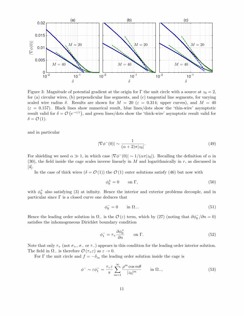
Figure 3: Magnitude of potential gradient at the origin for Γ the unit circle with a source at z0 = 2,for (a) circular wires, (b) perpendicular line segments, and (c) tangential line segments, for varyingscaled wire radius δ. Results are shown for M = 20 (ε = 0.314; upper curves), and M = 40(ε = 0.157). Black lines show numerical result, blue lines/dots show the ‘thin-wire’ asymptoticresult valid for δ = O

(e−c/ε

), and green lines/dots show the ‘thick-wire’ asymptotic result valid for

δ = O (1).

and in particular

|∇φ−(0)| ∼ 1

(α+ 2)π|z0|. (49)

For shielding we need α 1, in which case |∇φ−(0)| ∼ 1/(απ|z0|). Recalling the definition of α in(30), the field inside the cage scales inverse linearly in M and logarithmically in r, as discussed in[4].

In the case of thick wires (δ = O (1)) the O (1) outer solutions satisfy (46) but now with

φ±0 = 0 on Γ, (50)

with φ+0 also satisfying (3) at infinity. Hence the interior and exterior problems decouple, and in

particular since Γ is a closed curve one deduces that

φ−0 = 0 in Ω−. (51)

Hence the leading order solution in Ω− is the O (ε) term, which by (27) (noting that ∂φ−0 /∂n = 0)satisfies the inhomogeneous Dirichlet boundary condition

φ−1 = τ+∂φ+

0

∂non Γ. (52)

Note that only τ+ (not σ+, σ− or τ−) appears in this condition for the leading order interior solution.The field in Ω− is therefore O (τ+ε) as ε→ 0.

For Γ the unit circle and f = −δz0 the leading order solution inside the cage is

φ− ∼ εφ−1 =τ+ε

π

∞∑m=1

ρm cosmθ

|z0|min Ω−, (53)

11

and in particular

|∇φ−(0)| ∼ |τ+|επ|z0|

. (54)

In Figure 3 we show the excellent agreement between these approximations and the result ofnumerical calculations. Note that (49) and (54) are consistent, since τ+ ∼ 1/εα as δ → 0.

4.2 Helmholtz equation with Dirichlet boundary conditions on wires

In the thin wire case the analysis is similar to that for the Laplace case, with φ±0 satisfying

(∇2 + k2)φ+0 = f in Ω+, (∇2 + k2)φ−0 = 0 in Ω−, (55)

the boundary conditions (47), and an outgoing radiation condition on φ+0 .

For Γ the unit circle and f = −δz0 the leading order solution inside the cage is

φ− ∼ φ−0 =∞∑m=0

emJm(kρ) cosmθ

1 +α

k

(J ′m(k)Jm(k) −

H(1)m

′(k)

H(1)m (k)

)−1 in Ω−, (56)

where e0 = (i/4)H(1)0 (k|z0|) and em = (i/2)H

(1)m (k|z0|), m ∈ N. In particular

φ−(0) ∼i4H

(1)0 (k|z0|)

1 +α

k

(H

(1)1 (k)

H(1)0 (k)

− J1(k)J0(k)

)−1 . (57)

As in the Laplace case, the field strength is O (1/α) when α 1.In the thick wire case, at first glance the analysis appears similar to the Laplace case, with

the O (1) outer solutions satisfying (55) and (50). But now we must take care over the correctinterpretation of (50). This is because there exist resonant wavenumbers, i.e. values of k for whichk2 is a Dirichlet eigenvalue of −∇2 on Ω−, at which one cannot infer from (50) that φ−0 is identicallyzero. We shall study such resonant cases in detail in the next section. Here we simply record that,if we ignore resonance effects and assert that φ−0 = 0, the leading order solution in Ω− is againprovided by the O (ε) term, which satisfies (52), just as in the Laplace case.

For Γ the unit circle and f = −δz0 the leading order non-resonant solution inside the cage is

φ− ∼ εφ−1 = kετ+

∞∑m=0

em

(J ′m(k)

Jm(k)− H

(1)m

′(k)

H(1)m (k)

)Jm(kρ) cosmθ in Ω−, (58)

where em are as above. In particular

φ−(0) ∼ kετ+i

4H

(1)0 (k|z0|)

(H

(1)1 (k)

H(1)0 (k)

− J1(k)

J0(k)

). (59)

When one compares the approximations (57) and (59) with numerical simulations for fixed kaway from resonance, one observes similar behaviour to that in Figure 3, i.e. (57) is accurate forsmall δ and (59) for larger δ. However, interesting new behaviour become apparent when one fixesδ and varies the wavenumber k. Two plots of this type are presented in Figure 4. One finds thatclose to resonant wavenumbers the numerical solution is strongly peaked, and the amplitude |φ(0)|

12

0 1 2 3 4 5 6

|φ(0)|

0

0.1

0.2

0.3

0.4

0.5(a) δ = 0.01

k

0 1 2 3 4 5 6

|φ(0)|

0

0.1

0.2

0.3

0.4

0.5(b) δ = 0.1

2.3 2.5

0.5

1

1.5

2

2.5

5.4 5.6

0.5

1

1.5

2

2.5

Figure 4: Amplitudes at z = 0 for the wave problem for disk-shaped wires arranged around theunit circle, for varying wavenumber k. Corresponding field plots for particular wavenumbers areshown in Figure 5. Parameters are M = 30, z0 = 2, and (a) δ = 0.01, (b) δ = 0.1. Black linesshow the numerical solution, blue lines show the ‘thin-wire’ asymptotic result, green lines showsthe ‘thick-wire’ asymptotic result (without correcting for resonance), and the dotted line showsthe unshielded (free-field) solution. Vertical grey dashed lines indicate the unperturbed resonancesfor the unit circle corresponding to axisymmetric modes (two asymmetric modes are also excitedin this wavenumber range, but have zero amplitude at the origin), and red dashed lines show theshifted resonances calculated using the O (ε) perturbation in §44.3. Insets in the lower panel showenlargements around the peaks.

can actually exceed that of the free-field solution; that is, the cage amplifies the field rather thanshielding from it. This amplification is clear in the near-resonant field plots in Figure 5.

Returning to Figure 4, we note that the position of the peak amplitude is in general slightlyshifted from the exact resonance. For sufficiently small δ (cf. Figure 4(a)) the peaks are capturedcorrectly by the ‘thin-wire’ asymptotic result. But for larger δ the position and height of the peakare not predicted correctly (cf. Figure 4(b)). Unfortunately the ‘thick wire’ approximation (58)cannot capture the peaks either - the O (ε) term φ−1 blows up to infinity at the exact resonances, asis obvious from (58), and our asymptotic solution breaks down. In the next section we show how the‘thick wire’ approximation (59) can be modified to correctly predict the near-resonant behaviour forlarger values of δ.

4.3 Resonance effects

Close to resonant wavenumbers, our thick wire (δ = O (1)) solution (58) breaks down, as theassertion that φ−0 = 0 is invalid. Instead, we expect a near-resonant response in which the leadingorder interior solution is a non-trivial linear combination of the corresponding eigenmodes.

To examine the behaviour close to resonance, let k = k∗ + εk, where k∗ > 0 is a resonantwavenumber with real-valued eigenmode ψ satisfying (∇2 + k2

∗)ψ = 0 in Ω− and ψ = 0 on Γ,

13

Figure 5: (a)-(d) Numerical solutions to the wave problem for disk-shaped wires arranged aroundthe unit circle, for four different wavenumbers k, showing <(φ(z)). Parameters are M = 30, δ = 0.1,and z0 = 2. (b)-(d) represent near-resonant cases: in (b) and (c) the relevant resonant mode isJ0(k|z|), k ≈ 2.405, and in (d) it is J1(k|z|) cos(arg(z)), k ≈ 3.382. (e)-(h) ‘Thick-wire’ asymptoticsolutions for the same problems; in (e) this is the non-resonant solution (58), and in (f)-(h) we plotthe leading order resonance-corrected solution from §44.3, i.e. φ+

0 in Ω+ and φ−−1 in Ω−.

and k = O (1). (For simplicity we shall always assume there is only one eigenmode correspondingto k∗; more generally we would have a superposition of eigenmodes). Expanding (5) with φ =φ±0 + εφ±1 +O

(ε2)

as in (8), the leading order interior solution satisfies

(∇2 + k2∗)φ−0 = 0 in Ω−, (60)

φ−0 = 0 on Γ, (61)

whence

φ−0 = C0ψ, (62)

for some amplitude C0 to be determined. By (27) the next order interior problem is

(∇2 + k2∗)φ−1 = −2k∗kC0ψ in Ω−, (63)

φ−1 = τ+∂φ+

0

∂n− σ−C0

∂ψ

∂non Γ, (64)

where the inhomogeneous term on the right hand side of (63) arises from the perturbation of theeigenvalue from k∗. Since the associated homogeneous problem has a non-zero solution, ψ, there isa solvability condition to be satisfied, following from the identity∫

Ω−

ψ((∇2 + k2

∗)φ−1

)dS = −

∫Γφ−1

∂ψ

∂nds, (65)

14

which can be obtained using Green’s second identity. Defining

I1 =

∫Ω−

ψ2 dS, I2 =

∫Γ

(∂ψ

∂n

)2

ds, I3 =

∫Γκ

(∂ψ

∂n

)2

ds, (66)

(I3 is for later use), the solvability condition arising from (65) is that

(2k∗I1k + σ−I2)C0 = τ+

∫Γ

∂φ+0

∂n

∂ψ

∂nds. (67)

This determines the amplitude C0 of the O (1) interior solution (62), except when

k = k∗ := − σ−I2

2k∗I1, (68)

where C0 blows up to infinity. This represents a shift in the position of the apparent resonance fromthe original value k∗ to the perturbed value k∗+ εk∗. We note that the shift k∗ depends both on thewire shape K (through σ−) and on the cage geometry Γ (through I1 and I2). Furthermore, we notethat the sign of the shift is given by the sign of −σ−. For line segment wires parallel to Γ, σ− ispositive for all 0 < δ < 1/2, so the shift is always negative. But in general there may exist a criticalvalue of δ at which σ− (and hence the shift) changes sign. For circular wires this occurs at δ ≈ 0.12(cf. Figure 9).

The true solution is not actually infinite at the shifted value k = k∗ + εk∗; rather there is anarrow region of O

(ε2)

around this value in which the amplitude of the interior solution is large.

To capture this behaviour we write k = k∗ + εk∗ + ε2˜k, where k∗ is as in (68) and

˜k = O (1), and

introduce an extra leading term in the expansion of the interior solution,

φ−(x, y) =1

εφ−−1(x, y) + φ−0 (x, y) + εφ−1 (x, y) +O

(ε2)

in Ω−. (69)

As a result we require an additional O (1) term in the boundary layer solution, which becomes

Φ(N,S, s) =− ∂φ−−1

∂n(s)Φ−(N,S)− εκ(s)

∂φ−−1

∂n(s)Φ−(N,S)− ε∂

2φ−−1

∂n∂s(s)Φ−(N,S)

+ ε∂φ+

0

∂n(s)Φ+(N,S)− ε∂φ

−0

∂n(s)Φ−(N,S) +O

(ε2), (70)

where the functions Φ± and Φ± are defined in Appendix A. This solution is obtained from thegeneral solution to the boundary layer problem given in Appendix A, choosing the constants in thatsolution to match the gradients of the interior and exterior outer expansions. If φ−−1 = 0 it reducesto the solution given earlier. The resulting matching conditions for the outer solutions, analogousto (23)-(24), are

−(τ− − εκτ−)∂φ−−1

∂n− ετ−

∂2φ−−1

∂n∂s+ εσ+

∂φ+0

∂n− ετ−

∂φ−0∂n

= φ+0 + εφ+

1 on Γ, (71)

−(σ− − εκσ−)∂φ−−1

∂n− εσ−

∂2φ−−1

∂n∂s+ ετ+

∂φ+0

∂n− εσ−

∂φ−0∂n

=1

εφ−−1 + φ−0 + εφ−1 on Γ, (72)

where σ±, τ±, σ± and τ± are far field constants in the expansions of Φ± and Φ± (these constantsmay depend on the choice of wire model; see Appendix A).

15

The leading order interior problem for φ−−1 is identical to the earlier problem (60)-(61), withsolution

φ−−1 = C−1ψ, (73)

where C−1 is to be determined. This large interior solution causes a change to the leading orderexterior problem, for which the boundary condition (from (71)) becomes

φ+0 = −τ−C−1

∂ψ

∂non Γ. (74)

We split φ+0 into two components: one due to the source, and one forced by the boundary condition

(74), writing

φ+0 = φ+

0 + τ−C−1φ+0 , (75)

where (∇2 + k2∗)φ

+0 = f in Ω+ with φ+

0 = 0 on Γ and (∇2 + k2∗)φ

+0 = 0 in Ω+ with φ+

0 = −∂ψ/∂non Γ, with both φ+

0 and φ+0 satisfying outgoing radiation conditions at infinity.

The O (1) interior problem is

(∇2 + k2∗)φ−0 = −2k∗k∗C−1ψ in Ω−, (76)

φ−0 = −σ−C−1∂ψ

∂non Γ. (77)

The solvability condition is the same as (67) but with zero right-hand side and C0 replaced withC−1. This holds identically, given the definition of k∗ (cf. (68)), so the amplitude C−1 remainsundetermined at this order. Writing the solution to (76)-(77) as

φ−0 = σ−C−1φ−0 + C0ψ, (78)

where φ−0 is a particular solution of (∇2 + k2∗)φ−0 = (I2/I1)ψ in Ω− with φ−0 = −∂ψ/∂n on Γ, and

C0 is arbitrary, the O (ε) interior problem becomes

(∇2 + k2∗)φ−1 = −2k∗k∗C0ψ − C−1

(2k∗k∗σ−φ

−0 + (k2

∗ + 2k∗˜k)ψ

)in Ω−, (79)

φ−1 = τ+∂φ+

0

∂n− σ−C0

∂ψ

∂n+ C−1

(τ+τ−

∂φ+0

∂n− σ2

−∂φ−0∂n

+ κσ−∂ψ

∂n− σ−

∂2ψ

∂n∂s

)on Γ. (80)

Note that the right hand sides now contains terms due to the exterior field, as well as lower-ordercomponents of the interior field. The solvability condition is((

k2∗ + 2k∗

˜k)I1 − σ−I3 − τ+τ−I4 + σ2

−I5 + 2k∗k∗σ−I6

)C−1 = τ+I7, (81)

where

I4 =

∫Γ

∂φ+0

∂n

∂ψ

∂nds, I5 =

∫Γ

∂φ−0∂n

∂ψ

∂nds, I6 =

∫Ω−

φ−0 ψ dS, I7 =

∫Γ

∂φ+0

∂n

∂ψ

∂nds. (82)

In deriving (81) from (79) the C0 terms cancel due to (68), and the term proportional to σ− integratesto zero since Γ is a closed loop. Noting that I4 and I7 are in general complex, whereas I1, I3, I5

and I6 are real, the condition (81) determines C−1 with

|C−1| = |A|a(

(˜k − ˜

k∗)2 + a2

)−1/2, (83)

16

2.35 2.4

1

2

3

5.43 5.48

0.5

1

1.5

0 1 2 3 4 5 6

|φ(0)|

10-2

100

3.76 3.8

0.5

1

1.5

5.05 5.09

0.5

1

1.5

k

0 1 2 3 4 5 6

|φ(0.5)|

10-2

100

Figure 6: Amplitudes at z = 0 and z = 0.5 for the wave problem for disk-shaped wires arrangedaround the unit circle, for varying wavenumber k. Parameters are M = 30, δ = 0.1, and z0 = 2.Insets show enlargements of the regions close to resonance. Black line shows the numerical solution,blue line shows the ‘thin-wire’ asymptotic result, green line shows the non-resonant ‘thick-wire’asymptotic result, and red line shows the resonant thick-wire result. Vertical dashed lines indicatethe unperturbed resonances for the unit circle.

where

A =I7

τ−=(I4), a =

τ+τ−=(I4)

2I1k∗,

˜k∗ = −I1k

2∗ − σ−I3 − τ+τ−<(I4) + σ2

−I5 + 2k∗k∗σ−I6

2I1k∗. (84)

From (83) it follows that the maximum of |C−1| is |A| at˜k =

˜k∗. So, to conclude, the near-resonant

response occurs in a range of wavenumbers of width O(τ+τ−ε

2)

around k = k∗ + εk∗ + ε2˜k∗, and

the maximum amplitude is O (1/(τ−ε)). The exterior field remains O (1).The good agreement between these predictions and the result of numerical calculations is shown

in Figures 5, 6 and 7. The insets in figure 6 demonstrates that the shape of the amplitude variationwith wavenumber near the resonance is well captured, and Figure 7 demonstrates how the positionand amplitude at the peak vary with ε. We emphasise that as the number of wires increases, theresonant response occurs closer to the unperturbed resonant modes of Ω−, over an increasinglynarrow band of wavenumbers, but with an increasingly large amplitude.

4.4 Neumann solutions and resonance effects

For the equivalent problems satisfying Neumann conditions on the wires, we have seen in §3 thatthere is in general much weaker shielding than for Dirichlet conditions. Unless the gaps between thewires are small, the leading order homogenized solution does not notice the wires at all, and evenfor small gaps the homogenized wires provide a jump condition on Γ that does not necessarily leadto a weak field inside the cage. Only in the case of ‘very small gaps’ is there a significant shieldingeffect. Although this is not the main focus of our study (requiring very small gaps largely defeats

17

ε

0 0.05 0.1 0.15 0.2

kmax

2.2

2.25

2.3

2.35

2.4

2.45

2.5

δ =0.2

δ =0.1

δ =0.01

(a)

ε

0 0.05 0.1 0.15 0.2

Amax

0

5

10

15

20

25

30

δ =0.2

δ =0.1δ =0.01

(b)

Figure 7: (a) Wavenumbers giving maximum amplitude close to the first resonance for disk-shapedwires arranged around the unit circle, for varying ε (number of wires) and for different scaled wireradius δ, together with (b) the amplitude (at z = 0) for that wavenumber. Black lines/dots showmaxima from the numerical solutions, blue lines show the maxima from the ‘thin-wire’ asymptoticsolution, and red lines show the ‘thick-wire’ asymptotic result. The thin-wire result is not shown forδ = 0.2 since α < 0 in that case, so that approximation is invalid; for δ = 0.01, the thin wire resultis indistinguishable from the numerical solution in this plot.

the idea of a Faraday cage), we touch briefly on this very small gap case because of its analogyto the Dirichlet problems above. In particular, we focus on the perforated shell introduced in §3,for which the homogenized boundary conditions are (44) and (45), which depend on b2 ∼ ε2λ asdetermined from the solution to the boundary-layer cell problem.

For the Laplace problem, the O (1) solutions satisfy ∇2φ−0 = 0 subject to the homogenousNeumann conditions (44) on Γ. The interior solution φ−0 is therefore a constant, which is determinedfrom the solvability condition on the next-order problem: ∇2φ−1 = 0 with (45) on Γ. This determinesthe constant φ−0 to be the average of the exterior solution, φ+

0 , around Γ. The correction, whichcontrols the size of |∇φ(0)|, is O (1/(ελ)).

For the Helmholtz problem, theO (1) solutions satisfy (55) subject to homogenous Neumann con-ditions (26) on Γ. Away from resonance, the interior solution is φ−0 = 0, and the correction is againO (1/(ελ)). As for the Dirichlet problem, however, this solution breaks down if k is close to a resonantwavenumber k∗ for which there is a non-zero solution ψ to (∇2+k2

∗)ψ = 0 in Ω− with ∂ψ/∂n = 0 on Γ.The resonant case can be analysed in an equivalent fashion to the Dirichlet problem. Without givingthe details, we find that the wavenumber is shifted to k = k∗+(1/ελ) I2/4k∗I1 +O

(1/(ελ)2

), where

I1 and I2 are as defined in (66) for the relevant eigenfunction, while the peak amplitude at the originis O (ελ). Recall that in terms of the scaled gap size 1/2− δ, we have ελ ∼ (ε/π) log(1/(π(1

2 − δ))),so this resonant amplitude grows logarithmically as the size of the gaps is reduced.

5 Discussion and Conclusions

We have derived homogenized boundary conditions for various instances of the two-dimensionalFaraday cage problem, helping to quantify the effect of a wire mesh on electrostatic and electro-magnetic shielding. We have given an overview in §3 of the different leading order behaviour that

18

can occur depending on the scaled wire size δ, extending previous results for the ‘thin wire’ regimeδ 1, and incorporating the effects of finite wire size that in general allow for better shielding.The homogenized conditions help to clarify how the wire geometry affects the shielding behaviour,through the solution of cell problems and extraction of far-field constants. This allows us to makesome general comments on the shielding efficiency of different wires. For brevity we focus mainlyon the case of Dirichlet boundary conditions.

In the Dirichlet case, we showed that when the exterior wave field is O (1), the interior field isgenerally O (τ+ε), where ε = |Γ|/M and τ+ encodes the wire geometry. For thin wires we establishedthe approximation (21) for τ+, which indicates that the logarithmic capacity of the wires (controlledby their size and shape) is the key property governing shielding. For thicker wires, the orientationof the wires also becomes important, and the parameter τ+ can become small when the gap betweenwires is small. In this regime the relationship between the gap thickness (expressed as a fraction ofthe length of Γ) and the size of τ+ is strongly dependent on the wire shape. For example τ+ = 0.01is achieved with a gap thickness of approximately 0.22 for tangential line segments, but as much as0.54 for circular wires, and 0.61 for square wires. (For perpendicular line segments, the gap thicknessis always 1, but a wire length of 2δ ≈ 1.12 is required to achieve a correspondingly small value ofτ+).

We also derived a model for resonance effects in Faraday cages, showing how the incident exteriorwave field can be amplified by the presence of the cage in a narrow range of wavenumbers close tothe resonant wavenumbers for the corresponding solid shell. The analysis showed that at its peakthis resonance gives rise to a wave field O (1/(τ−ε)) larger than the incident field, and that thisoccurs over a range of wavenumbers of width O

(τ−τ+ε

2).

A similar analysis applies for a source inside the cage, when it is desired to shield the exteriorregion (as for a microwave oven, for example). In that case, for the ‘thick-wire’ regime, awayfrom resonance the interior solution is O (1) and the exterior field is O (τ−ε). Resonance occursat the same shifted eigenvalues as for the exterior source problem, but the peak amplitude is nowO(1/(τ−τ+ε

2)), and the corresponding radiated field outside the cage is O (1/(τ+ε)). (The relative

change in field strength from the non-resonant case is the same as in the case of an exterior source).Essentially the same analysis as in §44.3 can be followed, with the same result except that (83) givesthe amplitude of the O

(1/ε2

)interior solution, and the forcing term τ+I7 in (84) is replaced with

I8 =

∫Ω−

fψ dS. (85)

Although our homogenized boundary conditions were derived for smooth cages Γ, applying theresulting models to non-smooth geometries appears to give reasonable results, at least in terms ofcomputing resonance shifts and amplitudes. As an example of both this, and the interior source, weconsider a cage of circular wires arranged on a unit square, with a point source located inside thecage at z = −0.5. Numerical solutions illustrating the resonance effects are shown in Figure 8.

The unperturbed resonances for this problem are k∗ = (π/2)(l2 +m2)1/2, l, n ∈ N, for which

I1 = 1, I2 =π

2(l2 +m2)1/2. (86)

To calculate amplitude and corrections, we need to solve for I4 and I8. For the first resonance(l = m = 1), numerical solution of the relevant exterior problem for φ+

0 (performed using theMPSpack software package, which implements the non-polynomial finite element method of [2]) givesI4 ≈ 3.00− 16.02i, while I8 = 1/

√2. As Figure 8 shows, the analysis appears to capture the O (ε)

resonance shift correctly, as well as the O(1/ε2

)variation of the peak amplitude. To gain more

accuracy in the resonance shift we expect it would be necessary to consider local approximations in

19

Figure 8: Solutions for the wave problem for disk-shaped wires arranged around the unit square withsource at z0 = −0.5. (a) Numerically calculated amplitudes of the wave field at z = 2 for varyingwavenumber k, with parameters M = 32 (ε = 0.125), δ = 0.1. Vertical grey dashed lines indicatethe unperturbed resonances for the unit square, and red dashed lines show the shifted resonancescalculated using the O (ε) perturbation from (68). (b) Wavenumber giving maximum amplitudeclose to the first resonance for varying ε, together with (c) the maximum amplitude (at z = 0) forthat wavenumber. Black lines/dots show maxima from the numerical solutions, red lines show theasymptotic solutions for k∗+εk∗ from (68) and for I8/(τ−τ+ε

2=(I4)) from (84) with the modificationin (85). (d)-(e) Example numerical solutions showing <(φ(z)), away from resonance, and close toone of the resonant wavenumbers.

the vicinity of the corners (which were neglected in our anlaysis) and match these to the boundarylayer and outer expansions, following the procedure outlined in [18, 19, 12].

Our analysis of the Neumann problem shows that, as one might expect, Neumann wires shieldmuch less effectively than Dirichlet wires of the same size and shape. For the acoustic problemthis implies that it is very difficult to shield noise using a mesh-like structure made of sound-hardmaterial unless the gaps are very small. The implication for the electromagnetic problem is thata cage of parallel wires may provide reasonable shielding of waves whose electric field is polarizedparallel to the wire axes, but will not shield waves whose electric field is polarized perpendicular tothe wires axes. This effect is the basis of many polarizing filters, and explains, at least intuitively,why the mesh in the doors of microwave ovens is made of a criss-cross wire pattern or a perforatedsheet, rather than from parallel wires aligned in a single direction. However, a proper treatment ofthe full 3D electromagnetic case is left for future work.

6 Funding

IJH is supported by a Marie Curie FP7 Career Integration Grant within the 7th European UnionFramework Programme.

20

7 Acknowledgements

The authors gratefully acknowledge helpful discussions with Nick Trefethen, Jon Chapman, MikaelSlevinsky and Alex Barnett.

References

[1] V. M. Babich and V. S. Buldyrev, Short-Wavelength Diffraction Theory, Springer, Berlin,1991.

[2] A. H. Barnett and T. Betcke, An exponentially convergent nonpolynomial finite elementmethod for time-harmonic scattering from polygons, SIAM J. Sci. Comp., 32 (2010), pp. 1417–1441.

[3] M. Bruna, S. J. Chapman, and G. Z. Ramon, The effective flux through a thin-film com-posite membrane, EPL-Europhys. Lett., 110 (2015), p. 40005.

[4] S. J. Chapman, D. P. Hewett, and L. N. Trefethen, Mathematics of the Faraday cage,SIAM Rev., 57 (2015), pp. 398–417.

[5] D. Cioranescu and F. Murat, A strange term coming from nowhere, in Topics in theMathematical Modelling of Composite Materials, Progr. Nonlinear Differential Equat. Appl., 30(1997), pp. 45–93.

[6] X. Claeys and B. Delourme, High order asymptotics for wave propagation across thinperiodic interfaces, Asymptot. Anal., 83 (2013), pp. 35–82.

[7] D. G. Crowdy, Frictional slip lengths and blockage coefficients, Phys. Fluids, 23 (2011).

[8] , Uniform flow past a periodic array of cylinders, Eur. J. Mech. B-Fluid, 56 (2016), pp. 120–129.

[9] B. Delourme, Modeles et asymptotiques des interface fines et periodiques en eletromagnetisme,PhD thesis, U. Pierre et Marie Curie, 2010.

[10] B. Delourme, H. Haddar, and P. Joly, Approximate models for wave propagation acrossthin periodic interfaces, J. Math. Pures Appl., 98 (2012), pp. 28–71.

[11] , On the well-posedness, stability and accuracy of an asymptotic model for thin periodicinterfaces in electromagnetic scattering problems, Math. Mod. Meth. Appl. Sci., 23 (2013),pp. 2433–2464.

[12] B. Delourme, K. Schmidt, and A. Semin, High order asymptotic expansion for thin periodiclayers in polygonal domains, Proceedings of Waves 2015: the 12th International Conference onMathematical and Numerical Aspects of Wave Propagation, (2015), pp. 396–397.

[13] M. Faraday, Experimental Researches in Electricity, v.1, reprinted from Philosophical Trans-actions of 1831–1838, Richard and John Edward Taylor, London, 1839 (paragraphs 1173–4);available at www.gutenberg.org/ebooks/14986.

[14] R. Feynman, R. B. Leighton, and M. Sands, The Feynman Lectures on Physics, v. 2:Mainly Electromagnetism and Matter, Addison-Wesley, 1964.

21

[15] P. A. Martin, On acoustic and electric Faraday cages, Proc. Roy. Soc. A, 470 (2014),p. 20140344.

[16] P. A. Martin and R. A. Dalrymple, Scattering of long waves by cylindrical obstacles andgratings using matched asymptotic expansions, J. Fluid Mech., 188 (1988), pp. 465–490.

[17] J. C. Maxwell, A Treatise on Electricity and Magnetism, v.1, secs. 203–205, ClarendonPress, 1881.

[18] S. A. Nazarov, Dirichlet problem in an angular domain with rapidly oscillating boundary:modeling of the problem and asymptotic of the solution, St Petersburg Math. J., 19 (2008),pp. 297–326.

[19] , The Neumann problem in angular domains with periodic and parabolic perturbations ofthe boundary, Tr. Mosk. Mat. Obs., 69 (2008), pp. 182–241.

[20] T. Ransford, Potential Theory in the Complex Plane, Cambridge University Press, 1995.

[21] J. Rauch and M. Taylor, Electrostatic screening, J. Math. Phys., 16 (1975), pp. 284–288.

[22] , Potential and scattering theory on wildly perturbed domains, J. Func. Anal., 18 (1975),pp. 27–59.

[23] R. M. Slevinsky and S. Olver, A fast and well-conditioned spectral method for singularintegral equations, arXiv:1507.00596, (2015).

[24] L. N. Trefethen, Ten digit algorithms, Oxford technical report, (2005).

[25] E. O. Tuck, Matching problems involving flow through small holes, in Advances in AppliedMechanics, ed. Chia-Shun Y., vol. 15, Academic Press, 1975, ch. 2, pp. 89–158.

A Higher order boundary layer expansions

In this section we outline the derivation of the two-term boundary layer expansion

Φ(N,S; s) = Φ0(N,S; s) + εΦ1(N,S; s) +O(ε2), (87)

extending the leading order analysis given in §3. The higher-order expansion is required for ouranalysis of near-resonance effects in the Dirichlet case, and the ‘small gap’ regime in the Neumanncase. We begin by noting that the two-term boundary layer equation generalising (12) is

∂2Φ

∂N2+∂2Φ

∂S2+ εκ

(∂Φ

∂N− 2N

∂2Φ

∂S2

)+ 2ε

∂2Φ

∂S∂s+O

(ε2)

= 0. (88)

and the periodicity condition remains (13). The cell domain on which (88) is to hold is different forthe two wire models. For Model 2, when the wire shape is defined in the curvilinear coordinates,it is simply B = (N,S) : |S| < 1/2 \ K, where K = δK, and homogenous Dirichlet or Neumannboundary conditions (as appropriate) are imposed on the scaled wire boundary ∂K.

For Model 1, the curvature of Γ complicates matters somewhat. A priori the domain is Bε =(N,S) : |S| < 1/2 \ Kε, where Kε is the scaled wire described in (N,S) coordinates, and theboundary conditions are to be imposed on Kε. As illustrated in Figure 1, Kε is in general perturbedfrom K, depending on ε and the local curvature of Γ. This is undesirable, and it is preferable to

22

solve cell problems on the fixed cell domain B = (N,S) : |S| < 1/2 \ K, as for Model 2. If weonly desire the leading order approximation of Φ(N,S; s), as in the main text, the change from Bεto B incurs no loss of asymptotic accuracy. But when higher order terms are required, one needs toexpand the boundary conditions carefully so as to compensate for the geometric deformation.

To do this, note that the relationship (x, y) = Fj(n, s) between the local curvilinear and Cartesiancoordinates, introduced in §2, can be written in terms of the boundary-layer coordinates (N,S) as

x/ε = N − 12εκS

2 +O(ε2), y/ε = S + εκNS +O

(ε2), (89)

as ε→ 0, where κ = κ(s) is the local curvature of Γ. We suppose for definiteness that the boundaryof the reference wire shape, ∂K, is smooth and is given by W (ξ, η) = 0 in Cartesian coordinates(ξ, η) (cf. Figure 1(c)). The boundary ∂K is then given by W (N/δ, S/δ) = 0 (this is the actual wireboundary under Model 2), while ∂Kε is given by W (x/δε, y/δε) = 0. Expanding this expressionusing (89) shows that the Dirichlet condition Φ(N,S) = 0 on ∂Kε can be replaced by

Φ(N,S) + εκ d∂Φ

∂ν(N,S) +O

(ε2)

= 0 on ∂K, (90)

where κ(s) d(N,S) is the normal perturbation of ∂Kε from ∂K, with

d(N,S) = (12S

2,−NS) · ν, (91)

where ν = (νN , νS) = ∇W/|∇W | is the outward unit normal to ∂K.A more involved calculation shows that the Neumann condition ∂Φ/∂ν(N,S) = 0 on ∂Kε can

be replaced by

∂Φ

∂ν(N,S) + εκ

(d∂2Φ

∂ν2(N,S) + d

∂Φ

∂ν⊥(N,S)

)+O

(ε2)

= 0 on ∂K, (92)

with

d(N,S) = −S +NνNνS − κ∂K(N,S) (12S

2,−NS) · ν⊥, (93)

where ν⊥ = (−νS , νN ) is the (counterclockwise) unit tangent vector on ∂K, and κ∂K(N,S) is thecurvature of ∂K at the point (N,S). (The normal to ∂Kε is given by ν + εκ d(N,S)ν⊥ +O

(ε2).)

As a concrete example, consider the circular disc, when W (ξ, η) = ξ2+η2−1. Parameterising ∂Kby (N,S) = δ(cosϑ, sinϑ) for ϑ ∈ [0, 2π) gives ν = (cosϑ, sinϑ), κ∂K = 1/δ, d = −1

2δ2 cosϑ sin2 ϑ,

and d = δ sinϑ(1− 32 sin2 ϑ).

To summarise, the boundary-layer problems for Model 1 are given by (88) with periodic boundaryconditions (13), one of (90) or (92), and matching conditions as N → ±∞. The problems for Model2 are the same except that the geometric correction terms involving d and d in (90) and (92) areignored. We proceed with the analysis for Model 1, but note that the corresponding solutions forModel 2 can be obtained simply by setting d = d = 0 in the following.

A.1 Dirichlet problem

For the Dirichlet problem the leading order solution has the general form

Φ0(N,S; s) = A+0 (s)Φ+(N,S) +A−0 (s)Φ−(N,S), (94)

where Φ+ and Φ− are the canonical solutions defined earlier in (15)-(18).

23

The O (ε) solution can be written as

Φ1(N,S; s) = A+1 (s)Φ+ +A−1 (s)Φ− + κ(s)A+

0 Φ+ + κ(s)A−0 Φ− +∂A+

0

∂sΦ+ +

∂A−0∂s

Φ−, (95)

where Φ± and Φ± satisfy canonical problems defined in terms of Φ±. The problem for Φ± is

∂2Φ±

∂N2+∂2Φ±

∂S2= −2N

∂2Φ±

∂N2− ∂Φ±

∂Nin B (96)

Φ±(N,−1/2) = Φ±(N, 1/2), (97)

Φ± = −d(N,S)∂Φ±

∂νon ∂K, (98)

Φ+(N,S) ∼−1

2N2 + σ+, N →∞,

τ+, N → −∞,Φ−(N,S) ∼

−τ−, N →∞,12N

2 − σ−, N → −∞,(99)

where the constants σ± and τ± are determined as part of the solution. If the wire shape K issymmetric in ξ, then from (19) it follows that Φ+(N,S) = −Φ−(−N,S), so τ− = τ+, σ− = σ+.

The problem for Φ± is

∂2Φ±

∂N2+∂2Φ±

∂S2= −2

∂Φ±

∂Sin B, (100)

Φ±(N,−1/2) = Φ±(N, 1/2), (101)

Φ± = 0 on ∂K, (102)

Φ+(N,S) ∼σ+, N →∞,τ+, N → −∞,

Φ−(N,S) ∼τ−, N →∞,σ−, N → −∞,

(103)

where the constants σ± and τ± are again determined as part of the solution. If K is symmetric inξ then Φ+(N,S) = Φ−(−N,S), so τ− = τ+ and σ− = σ+.

The far-field behaviour as N → ±∞ of the two-term solution (87), required for matching, isthen

Φ ∼∓ 12εκA

±0 N

2 ± (A±0 + εA±1 )N +A±0 σ± +A∓0 τ∓

+ εA±1 σ± + εA∓1 τ∓ ± εκA±0 σ± ∓ εκA∓0 τ∓ + ε∂A±0∂s

σ± + ε∂A∓0∂s

τ∓ +O(ε2). (104)

A.2 Neumann problem

For the Neumann problem the O (ε) solution can be written as

Φ0(N,S; s) + εΦ1(N,S; s) = A0(s) + ε(A1(s) +B1(s)Ψ(N,S)

), (105)

where Ψ is the solution of the canonical problem defined in (32)-(35).The O

(ε2)

solution can be written as

Φ2(N,S; s) = A2(s) +B2(s)Ψ + κ(s)B1Ψ +∂B1

∂sΨ +

(∂2A0

∂s2+ k2A0

)Ψ, (106)

24

where Ψ(N,S) and Ψ(N,S) satisfy canonical problems involving Ψ(N,S), and Ψ(N,S) satisfies acanonical correction problem arising from the constant solution. The problem for Ψ(N,S) is

∂2Ψ

∂N2+∂2Ψ

∂S2= −2N

∂2Ψ

∂N2− ∂Ψ

∂Nin B (107)

Ψ(N,−1/2) = Ψ(N, 1/2), (108)

∂Ψ

∂ν= −d(N,S)

∂2Ψ

∂ν2− d(N,S)

∂Ψ

∂ν⊥on ∂K, (109)

Ψ(N,S) ∼ −12N

2 ± µN ± λ, N → ±∞, (110)

where the constants µ and λ are determined as part of the solution. If K is symmetric in ξ thenΨ(N,S) = −Ψ(−N,S), so that Ψ(N,S) = Ψ(−N,S) and λ = 0.

The constant µ arising here can be evaluated directly from Ψ, by integrating (107) over Band using the divergence theorem, which yields, after application of the boundary and matchingconditions, the formula

µ = λ− 1

2

∫∂K

[(Ψ− 2N

∂Ψ

∂N

)νN + d(N,S)

∂2Ψ

∂ν2+ d(N,S)

∂Ψ

∂ν⊥

]dν⊥. (111)

The problem for Ψ(N,S) is

∂2Ψ

∂N2+∂2Ψ

∂S2= −2

∂Ψ

∂Sin B, (112)

Ψ(N,−1/2) = Ψ(N, 1/2), (113)

∂Ψ

∂ν= 0 on ∂K, (114)

Ψ(N,S) ∼ ±µN ± λ, N → ±∞, (115)

where, again, the constants µ and λ are determined as part of the solution. If K is symmetric in ξthen Ψ(N,S) = −Ψ(−N,S) and µ = 0.

Finally, the problem for Ψ(N,S) is

∂2Ψ

∂N2+∂2Ψ

∂S2= −1 in B, (116)

Ψ(N,−1/2) = Ψ(N, 1/2), (117)

∂Ψ

∂ν= 0 on ∂K, (118)

Ψ(N,S) ∼ −12N

2 ± µN ± λ, N → ±∞, (119)

If K is symmetric in ξ then Ψ(N,S) = Ψ(−N,S) and λ = 0. Integrating (116) over B, as before,yields the formula µ = 1

2Area(K) [16].The far-field behaviour as N → ±∞ of (87) is then

Φ ∼− 12ε

2κB1N2 − 1

2ε2

(∂2A0

∂s2+ k2A0

)N2

+

(εB1 + ε2B2 ± ε2κµB1 ± ε2∂B1

∂sµ± ε2

(∂2A0

∂s2+ k2A0

)µ

)N

+A0 + εA1 ± εB1λ+ ε2A2 ± ε2B2λ± ε2κλB1 ± ε2∂B1

∂sλ± ε2

(∂2A0

∂s2+ k2A0

)λ+O

(ε3).

(120)

25

Figure 9: Solutions to the cell problem (15)-(18) for (a) disk-shaped wires with radius δ, (b) infinitelythin perpendicular line segments with length 2δ, and (c) square wires with side length

√2δ. Upper

panels show contours of Φ+(N,S) for δ = 0.2. Lower panels show the constants σ and τ in thefar field expansion, as a function of δ. Dashed lines show asymptotic behaviour of σ and τ as δapproaches 0 and 1

2 (or δ →∞ in (b)). In (a), the higher-order correction σ from (99) is also shown,for Model 1 (solid) and Model 2 (dashed), and in (c) the magenta curve shows σ = τ for a tangentialline segment of length 2δ, from (124).

B Cell problem solutions

In this section we present numerical and analytical solutions to the leading order boundary layercell problems for disk-shaped, perpendicular/tangential line segments, and square wires.

B.1 Dirichlet problems

Example solutions for the Dirichlet cell problem (15)-(18) are shown in Figure 9, along with plotsof the corresponding far-field constants σ = σ± and τ = τ±.

The solutions for circular wires in Figure 9(a) are calculated numerically using linear finiteelements, with the constants σ and τ found from a linear fit of the far-field behaviour. For smallwires, δ → 0, we recall the asymptotic behaviour (20)-(21). For δ = δmax = 1

2 , the circle takes upthe whole width of the cell domain and Φ+ = 0 for X < 0 (so τ = 0), while a numerical solutiongives σ ≈ −0.44 for the constant as X → ∞. As δ → 1

2 , the asymptotic behaviour of σ can befound by solving a perturbation problem numerically, from which we obtain σ ∼ −0.44+1.07(1

2−δ),while τ is exponentially small. The solutions for the square wire in Figure 9(c) were also computednumerically; we note that in this case δmax = 1/

√2.

Solutions for the two arrangements of line segments can be found analytically by conformalmapping. For the wires arranged perpendicular to Γ we obtain

Φ+(N,S) = <

1

2πlog

[e−πδ + ζ

e−πδ − ζ

], ζ =

[sinhπ(Z − δ)sinhπ(Z + δ)

]1/2

, Z = N + iS, (121)

26

Figure 10: Solutions to the Neumann cell problem (32)-(35) for (a) disk-shaped wires with radius δ,(b) infinitely thin line segments with length 2δ, and (c) square wires with side length

√2δ. Upper

panels show contours of Ψ(N,S) for δ = 0.3. Lower panels show the constant λ in the far fieldexpansion, as a function of δ. The dashed lines in (a) show the approximations λ ∼ πδ2 andλ ∼ πδ2/(1− (πδ)2/3) [8], and in (b) show the behaviour as δ approaches 0 and 1

2 .

from which we find

σ = − 1

2πlog

(sinh 2πδ

2

), τ = − 1

2πlog (tanhπδ) . (122)

These have limiting behaviour σ ∼ τ ∼ −(1/2π) log(πδ) as δ → 0 (so that in particular a0 = log 2),and σ ∼ −δ + (1/π) log 2, τ ∼ (1/π)e−2πδ as δ →∞, as shown in Figure 9(b).

For the wires arranged tangentially along Γ we obtain

Φ+(N,S) = <

1

2πlog

[eiπδ + ζ

e−iπδ − ζ

], ζ =

[sinπ(iZ + δ)

sinπ(iZ − δ)

]1/2

, Z = N + iS, (123)

from which we find

σ = τ = − 1

2πlog (sinπδ) . (124)

This again has σ ∼ τ − (1/2π) log(πδ) as δ → 0 (so a0 = log 2), while σ ∼ τ ∼ 14π(1

2 − δ)2 as δ → 12 .

B.2 Neumann problems

Example solutions for the Neumann cell problem (32)-(35) are shown in Figure 10.The circular wire case is again calculated numerically, although the asymptotic behaviour for

small and large circles provides a good fit over the whole range of δ. For δ → 0, the solution awayfrom the wire can be written approximately as

Ψ(N,S) ∼ <Z +

δ2π

tanhπZ

, Z = N + iS, (125)

27

which gives λ ∼ πδ2 as δ → 0. (The strength of the singularity here is again determined by matchingto an inner region close to the wire, as in [4, §B], where Ψ ∼ <

Z + δ2/Z

). We remark that the

analysis in [8] provides a more refined approximation λ ∼ (πδ2)/(1− (πδ)2/3), which is also plottedin Figure 10. For δ → 1

2π, one can show that λ ∼ 14π(1

2 − δ)−1/2.For line segments arranged perpendicular to Γ, the wire has no impact on the solution, which is

simply Ψ(N,S) = N , so λ = 0. For line segments arranged tangentially along Γ, conformal mappingyields

Ψ(N,S) = <

1

2πlog

[(eiπδ − ζ)(e−iπδ + ζ)

(e−iπδ − ζ)(eiπδ + ζ)

], ζ =

[sinπ(iZ + δ)

sinπ(iZ − δ)

]1/2

, Z = N + iS, (126)

from which we find

λ = − 1

πlog (cosπδ) . (127)

This has limiting behaviour λ ∼ 12πδ

2 as δ → 0, and λ ∼ −(1/π) log π(12 − δ) as δ → 1

2 . Using (126)in (111), for Model 2, we find that µ = 0, along with µ = 0 (by symmetry) and µ = 0.

28