A systematic study of the class imbalance problem

in convolutional neural networks

Mateusz Buda1, 2 Atsuto Maki2 Maciej A. Mazurowski1, 3

1Department of Radiology, Duke University School of Medicine, Durham, NC, USA2Royal Institute of Technology (KTH), Stockholm, Sweden

3Department of Electrical and Computer Engineering, Duke University, Durham, NC, USA

{buda, atsuto}@kth.se, maciej.mazurowski@duke.edu

Abstract

In this study, we systematically investigate the impact of class imbalance on clas-sification performance of convolutional neural networks (CNNs) and compare fre-quently used methods to address the issue. Class imbalance is a common problemthat has been comprehensively studied in classical machine learning, yet very lim-ited systematic research is available in the context of deep learning. In our study,we use three benchmark datasets of increasing complexity, MNIST, CIFAR-10 andImageNet, to investigate the effects of imbalance on classification and perform anextensive comparison of several methods to address the issue: oversampling, un-dersampling, two-phase training, and thresholding that compensates for prior classprobabilities. Our main evaluation metric is area under the receiver operating charac-teristic curve (ROC AUC) adjusted to multi-class tasks since overall accuracy metricis associated with notable difficulties in the context of imbalanced data. Based onresults from our experiments we conclude that (i) the effect of class imbalance onclassification performance is detrimental; (ii) the method of addressing class imbal-ance that emerged as dominant in almost all analyzed scenarios was oversampling;(iii) oversampling should be applied to the level that totally eliminates the imbalance,whereas undersampling can perform better when the imbalance is only removed tosome extent; (iv) as opposed to some classical machine learning models, oversamplingdoes not necessarily cause overfitting of CNNs; (v) thresholding should be appliedto compensate for prior class probabilities when overall number of properly classifiedcases is of interest.

Keywords: Class Imbalance, Convolutional Neural Networks, Deep Learning, ImageClassification

1 Introduction

Convolutional neural networks (CNNs) are gaining significance in a number of machinelearning application domains and are currently contributing to the state of the art in thefield of computer vision, which includes tasks such as object detection, image classification,and segmentation. They are also widely used in natural language processing or speech

1

arX

iv:1

710.

0538

1v1

[cs

.CV

] 1

5 O

ct 2

017

recognition where they are replacing or improving classical machine learning models [1].CNNs integrate automatic feature extraction and discriminative classifier in one model,which is the main difference between them and traditional machine learning techniques.This property allows CNNs to learn hierarchical representations [2]. The standard CNNis built with fully connected layers and a number of blocks consisting of convolutions,activation function layer and max pooling [3, 4, 5]. The complex nature of CNNs requiresa significant computational power for training and evaluation of the networks, which isaddressed with the help of modern graphical processing units (GPUs).

A common problem in real life applications of deep learning based classifiers is thatsome classes have a significantly higher number of examples in the training set thanother classes. This difference is referred to as class imbalance. There are plenty ofexamples in domains like computer vision [6, 7, 8, 9, 10], medical diagnosis [11, 12],fraud detection [13] and others [14, 15, 16] where this issue is highly significant and thefrequency of one class (e.g., cancer) can be 1000 times less than another class (e.g., healthypatient). It has been established that class imbalance can have significant detrimentaleffect on training of traditional classifiers [17] including multi-layer perceptrons [18]. Itaffects both convergence during the training phase and generalization of a model on thetest set. While the issue very likely also affects deep learning, no systematic study on thetopic is available.

Methods of dealing with imbalance are well studied for classical machine learningmodels [19, 17, 20, 18]. The most straightforward and common approach is the use ofsampling methods. Those methods operate on the data itself (rather than the model)to increase its balance. Widely used and proven to be robust is oversampling [21]. An-other option is undersampling. Naıve version, called random majority undersampling,simply removes a random portion of examples from majority classes [17]. The issue ofclass imbalance can be also tackled on the level of the classifier. In such case, the learn-ing algorithms are modified, e.g. by introducing different weights to misclassification ofexamples from different classes [22] or explicitly adjusting prior class probabilities [23].

Some previous studies showed results on cost sensitive learning of deep neural net-works [24, 25, 26]. New kinds of loss function for neural networks training were alsodeveloped [27]. Recently, a new method for CNNs was introduced that trains the net-work in two-phases in which the network is trained on the balanced data first and thenthe output layers are fine-tuned [28]. While little systematic analysis of imbalance andmethods to deal with it is available for deep learning, researchers employ some meth-ods that might be addressing the problem likely based on intuition, some internal tests,and systematic results available for traditional machine learning. Based on our review ofliterature, the method most commonly applied in deep learning is oversampling.

The rest of this paper is organized as follows. Section 2 gives an overview of methodsto address the problem of imbalance. In Section 3 we describe the experimental setup.It provides details about compared methods, datasets and models used for evaluation.Then, in Section 4 we present the results from our experiments and compare methods.Finally, Section 5 concludes the paper.

2

2 Methods for addressing imbalance

Methods for addressing class imbalance can be divided into two main categories [29]. Thefirst category is data level methods that operate on training set and change its class dis-tribution. They aim to alter dataset in order to make standard training algorithms work.The other category covers classifier (algorithmic) level methods. These methods keep thetraining dataset unchanged and adjust training or inference algorithms. Moreover, meth-ods that combine the two categories are available. In this section we give an overviewof commonly used approaches in both classical machine learning models and deep neuralnetworks.

2.1 Data level methods

Oversampling. One of the most commonly used method in deep learning [16, 30,31, 32]. The basic version of it is called random minority oversampling, which simplyreplicates randomly selected samples from minority classes. It has been shown that over-sampling is effective, yet it can lead to overfitting [33, 34]. More advanced samplingmethod that aims to overcome this issue is SMOTE [33]. It augments artificial examplescreated by interpolating neighboring data points. Some extensions of this technique wereproposed, for example focusing only on examples near the boundary between classes [35].Another type of oversampling approach uses data preprocessing to perform more informedoversampling. Cluster-based oversampling first clusters the dataset and then oversam-ples each cluster separately [36]. This way it reduces both between-class and within-classimbalance. DataBoost-IM, on the other hand, identifies difficult examples with boostingpreprocessing and uses them to generate synthetic data [37]. An oversampling approachspecific to neural networks optimized with stochastic gradient descent is class-aware sam-pling [38]. The main idea is to ensure uniform class distribution of each mini-batch andcontrol the selection of examples from each class.

Undersampling. Another popular method [16] that results in having the same numberof examples in each class. However, as opposed to oversampling, examples are removedrandomly from majority classes until all classes have the same number of examples. Whileit might not appear intuitive, there is some evidence that in some situations undersamplingcan be preferable to oversampling [39]. A significant disadvantage of this method is thatit discards a portion of available data. To overcome this shortcoming, some modificationswere introduced that more carefully select examples to be removed. E.g. one-sidedselection identifies redundant examples close to the boundary between classes [40]. Moregeneral approach than undersampling is data decontamination that can involve relabelingof some examples [41, 42].

2.2 Classifier level methods

Thresholding. Also known as threshold moving or post scaling, adjusts the decisionthreshold of a classifier. It is applied in the test phase and involves changing the outputclass probabilities. There are many ways in which the network outputs can be adjusted.

3

In general, the threshold can be set to minimize arbitrary criterion using an optimiza-tion algorithm [23]. However, the most basic version simply compensates for prior classprobabilities [43]. These are estimated for each class by its frequency in the imbalanceddataset before sampling is applied. It was shown that neural networks estimate Bayesiana posteriori probabilities [43]. That is, for a given datapoint x, their output for class iimplicitly corresponds to

yi(x) = p(i|x) =p(i) · p(x|i)

p(x).

Therefore, correct class probabilities can be obtained by dividing the network output for

each class by its estimated prior probability p(i) =∑

k |k||i| , where |i| denotes the number

of unique examples in class i.

Cost sensitive learning. This method assigns different cost to misclassification of ex-amples from different classes [44]. With respect to neural networks it can be implementedin various ways. One approach is threshold moving [22] or post scaling [23] that are ap-plied in the inference phase after the classifier is already trained. Similar strategy is toadapt the output of the network and also use it in the backward pass of backpropagationalgorithm [45]. Another adaptation of neural network to be cost sensitive is to modify thelearning rate such that higher cost examples contribute more to the update of weights.And finally we can train the network by minimizing the misclassification cost insteadof standard loss function [45]. The results of this approach are equivalent to oversam-pling [22, 26] described above and therefore this method will not be implemented in ourstudy.

One-class classification. In the context of neural networks it is usually called nov-elty detection. This is a concept learning technique that recognizes positive instancesrather than discriminating between two classes. Autoencoders used for this purpose aretrained to perform autoassociative mapping, i.e. identity function. Then, the classifica-tion of a new example is made based on a reconstruction error between the input andoutput patterns, e.g. absolute error, squared sum of errors, Euclidean or Mahalanobisdistance [46, 47, 48]. This method has proved to work well for extremely high imbalancewhen classification problem turns info anomaly detection [49].

Hybrid of methods. This is an approach that combines multiple techniques from oneor both abovementioned categories. Widely used example is ensembling. It can be viewedas a wrapper to other methods. EasyEnsemble and BalanceCascade are methods thattrain a committee of classifiers on undersampled subsets [50]. SMOTEBoost, on the otherhand, is a combination of boosting and SMOTE oversampling [51]. Recently introducedand successfully applied to CNN training for brain tumor segmentation, is two-phasetraining [28]. Even though the task was image segmentation, it was approached as a pixellevel classification. The method involves network pre-training on balanced dataset andthen fine-tuning the last output layer before softmax on the original, imbalanced data.

4

3 Experiments

3.1 Forms of imbalance

Class imbalance can take many forms particularly in the context of multiclass classi-fication, which is typical in CNNs. In some problems only one class might be under-represented or overrepresented and in other every class will have a different number ofexamples. In this study we define and investigate two types of imbalance that we believeare representative of most of the real-world cases.

The first type is step imbalance. In step imbalance, the number of examples is equalwithin minority classes and equal within majority classes but differs between the majorityand minority classes. This type of imbalance is characterized by two parameters. One isthe fraction of minority classes defined by

µ =|{i ∈ {1, . . . , N} : Ci is minority}|

N, (1)

where Ci is a set of examples in class i and N is the total number of classes. The otherparameter is a ratio between the number of examples in majority classes and the numberof examples in minority classes defined as follows.

ρ =maxi{|Ci|}mini{|Ci|}

(2)

An example of this type of imbalance is the situation when among the total of 10 classes,5 of them have 500 training examples and another 5 have 5 000. In this case ρ = 10 andµ = 0.5, as shown in Figure 1a. A dataset with the same number of examples in totalthat has smaller imbalance ratio, corresponding to parameter ρ = 2, but more classesbeing minority, µ = 0.9, is presented in Figure 1b.

(a) ρ = 10, µ = 0.5 (b) ρ = 2, µ = 0.9 (c) ρ = 10

Figure 1: Example distributions of imbalanced set together with corresponding values of param-eters ρ and µ for step imbalance (a - b) and ρ for linear imbalance (c).

The second type of imbalance we call linear imbalance. We define it with one param-eter that is a ratio between the maximum and minimum number of examples among allclasses, as in Equation 2 for imbalance ratio in step imbalance. However, the number ofexamples in the remaining classes is interpolated linearly such that the difference betweenconsecutive pairs of classes is constant. An example of linear imbalance distribution withρ = 10 is shown in Figure 1c.

5

3.2 Methods of addressing imbalance compared in this study

In total, we examine seven methods to handle CNN training on a dataset with classimbalance which cover most of the commonly used approaches in the context of deeplearning:

1. Random minority oversampling

2. Random majority undersampling

3. Two-phase training with pre-training on randomly oversampled dataset

4. Two-phase training with pre-training on randomly undersampled dataset

5. Thresholding with prior class probabilities

6. Oversampling with thresholding

7. Undersampling with thresholding

We examine two variants of two-phase training method. One on oversampled and theother on undersampled dataset. For the second phase, we keep the same hyperparametersand learning rate decay policy as in the first phase. Only the base learning rate fromthe first phase is multiplied by the factor of 10−1. Regarding thresholding, this methodoriginally uses the imbalanced training set to train a neural network. We, in addition,combine it with oversampling and undersampling.

Selected methods are representative of the available approaches. Sampling can beused to explicitly incorporate cost of the examples by their appearance. It makes themone of many implementations of cost-sensitive learning [22]. Thresholding is another wayof applying cost-sensitiveness by moving the output threshold such that higher cost exam-ples are harder to misclassify. Ensemble methods require training of multiple classifiers.Because of considerable time needed to train deep models, it is often not practical andmay be even infeasible to train multiple deep neural networks. One-class methods have avery limited application to datasets with extremely high imbalance. Moreover, they areapplied to anomaly detection problem that is beyond the scope of our study.

Importantly, we focused on methods that are widely used and relatively straightfor-ward to implement as our aim is to draw conclusions that will be practical and serve asa guidance to a large number of deep learning researchers and engineers.

3.3 Datasets and models

In our study, we used three benchmark datasets: MNIST [52], CIFAR-10 [53] and Im-ageNet Large Scale Visual Recognition Challenge (ILSVRC) 2012 [54]. All of them areprovided with a split on training and test set that are both labelled. For each dataset wechoose different model with a set of hyperparameters used for its training that is known toperform well based on the literature. Datasets together with their corresponding modelsare of increasing complexity. This allows us to draw some conclusions on simple task andthen verify how they scale to more complex ones.

All networks for the same dataset were trained with equal number of iterations. Itmeans that the number of epochs differs between the imbalanced versions of dataset. This

6

way we keep the number of weights’ updates constant. Also, all networks were trainedfrom a random initialization of weights and no pretraining was applied. An overview ofsome information about the datasets and their corresponding models is given in Table 1.All experiments were implemented in the deep learning framework Caffe [55].

Image dimensions Images per class

Dataset Width Height Depth No. classes Training Test CNN model

MNIST 28 28 1 10 5 000 1 000 LeNet-5CIFAR-10 32 32 3 10 5 000 1 000 All-CNN

ILSVRC-2012 ≥ 256 ≥ 256 3 1 000 1 000 50 ResNet-10

Table 1: Summary of the used datasets. The number of images per class refers to theperfectly balanced subsets used for experiments. Provided image dimensions for ImageNetare given after rescaling.

3.3.1 MNIST

MNIST is considered simple and solved problem that involves digits’ images classifica-tion. The dataset consists of grayscale images of size 28 × 28. There are ten classescorresponding to digits from 0 to 9. The number of examples per class in the originaltraining dataset ranges from 5421 in class 5 to 6742 in class 1. In artificially imbalancedversions we uniformly at random subsample each class to contain no more than 5 000examples.

Data dimensions

Layer Width Height Depth Kernel size Stride

Input 28 28 1 - -Convolution 24 24 20 5 1Max Pooling 12 12 20 2 2Convolution 8 8 50 5 1Max Pooling 4 4 50 2 2

Fully Connected 1 1 500 - -ReLU 1 1 500 - -

Fully Connected 1 1 10 - -Softmax 1 1 10 - -

Table 2: Architecture of LeNet-5 CNN used in MNIST experiments.

The CNN model that we use for MNIST is the modern version of LeNet-5 [52].The network architecture is presented in Table 2. All networks for this dataset weretrained for 10 000 iterations. Optimization algorithm is stochastic gradient descent (SGD)with momentum value of µ = 0.9 [56]. The learning rate decay policy is defined as

7

ηt = η0 · (1 + γ · t)−α, where η0 = 0.01 is a base learning rate, γ = 0.0001 and α = 0.75are decay parameters and t is the current iteration. Furthermore, we used a batch sizeof 64 and a weight decay value of λ = 0.0005. Network weights were initialized randomlywith uniform distribution and Xavier variance [57] whereas the biases were initializedwith zero. No data augmentation was used. Test error of the model trained as describedabove on the original MNIST dataset was below 1%.

Experiments on MNIST dataset are performed on the following imbalance parametersspace. For linear imbalance we test values of ρ ∈ {10, 25, 50, 100, 250, 500, 1 000, 2 500, 5 000}.For step imbalance the set of ρ values is the same and for each we use all possible number ofminority classes from 1 to 9, which corresponds to µ ∈ {0.1, 0.2, 0.3, 0.4, 0.5, 0.6, 0.7, 0.8, 0.9}.The experiment for each combination of parameters is repeated 50 times. Every time thesubset of minority classes is randomized. This way, we have created 4 050 artificiallyimbalanced training sets for step imbalance and 450 for linear imbalance. As we haveevaluated four methods that require training a model, the total number of trained net-works, including baseline, is 22 500.

3.3.2 CIFAR-10

CIFAR-10 is a significantly more complex image classification problem than MNIST. Itcontains 32 × 32 color images with ten classes of natural objects. It does not have anynatural imbalance at all. There are exactly 5 000 training and 1 000 test examples in eachclass. We do not use any data augmentation but follow standard preprocessing comprisingglobal contrast normalization and ZCA whitening [58].

Data dimensions

Layer Width Height Depth Kernel size Stride Padding

Input 32 32 3 - - -Dropout (0.2) 32 32 3 - - -

2×(Convolution + ReLU) 32 32 96 3 1 1Convolution + ReLU 16 16 96 3 2 1

Dropout (0.5) 16 16 96 - - -2×(Convolution + ReLU) 16 16 192 3 1 1

Convolution + ReLU 8 8 192 3 2 1Dropout (0.5) 8 8 192 - - -

Convolution + ReLU 6 6 192 3 1 0Convolution + ReLU 6 6 192 1 1 0Convolution + ReLU 6 6 10 1 1 0

Average Pooling 1 1 10 6 - -Softmax 1 1 10 - - -

Table 3: Architecture of All-CNN used in CIFAR-10 experiments.

For CIFAR-10 experiments we use one of the best performing type of CNN model onthis dataset, i.e. All-CNN [59]. The network architecture is presented in Table 3. The

8

networks were trained for 70 000 iterations using SGD with momentum µ = 0.9. The baselearning rate was multiplied by a fixed multiplier of 0.1 after 40 000, 50 000 and 60 000iterations. The number of examples in a batch was 256 and a weight decay value wasλ = 0.001. Network weights were initialized with Xavier procedure and the biases setto zero. Test error of the model trained as described above on the original CIFAR-10dataset was 9.75%.

We have found the network training to be quite sensitive to initialization and thechoice of base learning rate. Sometimes the network gets stuck in a very poor localminimum. Also, for more imbalanced datasets the training required lower base learningrate to train at all. Therefore, for each case we were searching for the best one from thefixed set η0 ∈ {0.05, 0.005, 0.0005, 0.00005}. Similar procedure was used by the authorsof the model architecture [59]. Moreover, each training was repeated twice on the samedataset. For a particular method and imbalanced dataset, we pick the model with thebest score on the test set over all eight runs.

The network architecture does not have any fully connected layers. Therefore, duringthe fine-tuning in two-phase training method we update the weights of two last convolu-tional layers with kernels of size 1.

The imbalance parameters space used in CIFAR-10 experiments is considerably sparserthan the one used for MNIST due to the significantly longer time required to train onenetwork. The set of tested values was narrowed to make the experiment run in a rea-sonable time. For linear and step imbalance, we test values of ρ ∈ {2, 10, 20, 50}. In stepimbalance, for each value of ρ, the set of values of parameter µ was µ ∈ {0.2, 0.5, 0.8},which corresponds to having two, five and eight minority classes respectively. And for allthe cases, the classes chosen to be minority were the ones with the lowest label value. Itmeans that for a fixed number of minority classes the same classes were always picked asminority. Also, all of them were included in a larger set of minority classes. In total wetrained 480 networks on this dataset.

3.3.3 ImageNet

For evaluation we use a ILSVRC-2012 competition subset of ImageNet, widely used asa benchmark to compare classifiers’ performance. The number of examples in majorityclasses was reduced from 1 200 to 1 000. Classes with less than 1 000 cases were alwayschosen as a minority ones for imbalanced subsets. The only data preprocessing appliedis resizing such that the smaller dimension is 256 pixels long and the aspect ratio ispreserved. During training, as input we use a randomly cropped 224 × 224 pixel squarepatch and a single centered crop in a test phase. Moreover, during training we randomlymirror images, but there is no color, scale or aspect ratio augmentation.

A model architecture employed for this dataset is ResNet-10 [60], i.e. a residualnetwork [61] with batch normalization layers that are known to accelerate deep networkstraining [62]. It consists of four residual blocks that give us nine convolutional layersand one fully connected. The first residual block outputs data tensor of depth 64 andthen each one increases it by a factor of two. Fully connected layer outputs 1 000 valuesto softmax that transforms them to class probabilities. The architecture of one residualblock is presented in Figure 2.

9

Figure 2: Architecture of a single residual block in ResNet used in ILSVRC-2012 experiments.

The networks were trained for 320 000 iterations using SGD with momentum µ = 0.9.The base learning rate is set to η0 = 0.1 and decays linearly to 0 in the last iteration. Thenumber of examples in a batch was 256 and a weight decay λ = 0.0001. Network weightswere initialized with Kaiming (also known as MSRA) initialization procedure [63]. Top-1test error of the model trained as described above on the original ILSVRC-2012 datasetwas 62.56% and 99.50 multi-class ROC AUC for a single centered crop.

We have chosen relatively small ResNet for the sake of faster training but withoutloss of generality 1. We test only one case of small and two cases of large step imbal-ance and run it on the baseline, undersampling and oversampling methods. Specifically,all three step imbalanced subsets are defined with µ = 0.1, ρ = 10, µ = 0.8, ρ = 50 andµ = 0.9, ρ = 100. They correspond to 100 minority classes with imbalance ratio of 10,800 minority classes with imbalance of 50, and 900 minority classes with imbalance ratioof 100 respectively. Moreover, for the highest imbalance, we train three networks for eachmethod with randomized selection of minority classes and subsampled set of examples ineach class. This is done in order to estimate variability in performance of methods. Intotal, this gives us 15 ResNet-10 networks trained on five artificially imbalanced subsetsof ILSVRC-2012.

3.4 Evaluation metrics and testing

The metric that is most widely used to evaluate a classifier performance in the con-text of multiclass classification with CNNs is overall accuracy which is the proportion oftest examples that were correctly classified. However, it has some significant and longacknowledged limitations, particularly in the context of imbalanced datasets [19]. Specifi-cally, when the test set is imbalanced, accuracy will favor classes that are overrepresentedin some cases leading to highly misleading assessment. An example of this is a situationwhen the majority class represents 99% of all cases and the classifier assigns the labelof the majority class to all test cases. A misleading accuracy of 99% will be assignedto a classifier that has a very limited use. Another issue might arise when the test setis balanced and a training set is imbalanced. This might result in a situation when adecision threshold is moved to reflect the estimated class prior probabilities and cause alow accuracy measure in the test set while the true discriminative power of the classifierdoes not change.

A measure that addresses these issues is area under the receiver operating character-istic curve (ROC AUC) [64]. It is a well-studied and sound measure of discrimination [65]

1It takes five days to train one ResNet-10 network on Nvidia GTX 1070 GPU.

10

and has been widely used as an evaluation metric for classifiers. ROC has also been usedto compare performance of classifiers trained on imbalanced datasets[20, 18]. Since thebasic version of ROC is only suitable for binary classification, we use a multi-class modi-fication of it by averaging ROC AUCs for the binary classification task of distinguishinga given class vs. all the other classes [66].

Test set of all used datasets has equal number of examples in each class. Usually, it isassumed that the class distribution of a test set follows the one of a training set. We donot change a test set to match artificially imbalanced training set. The reason is that thescore achieved by each classifier on the same test set is more comparable and the largestnumber of cases in each of the classes provides the most accurate performance estimation.

4 Results

4.1 Effects of class imbalance on classification performance and com-parison of methods to address imbalance

The results showing the impact of class imbalance on classification performance andcomparison of methods for addressing imbalance are shown in Figures 3 and 4. Figure 3shows the results with respect to multi-class ROC AUC for a fixed number of minorityclasses on MNIST and CIFAR-10. Figure 4 presents the result from the perspective offixed ratio of imbalance, i.e. parameter ρ, for the same two datasets.

(a) 2 minority classes (b) 5 minority classes (c) 8 minority classes

(d) 2 minority classes (e) 5 minority classes (f) 8 minority classes

Figure 3: Comparison of methods with respect to multi-class ROC AUC on MNIST (a - c) andCIFAR-10 (d - f) for step imbalance with fixed number of minority classes.

11

Regarding the effect of class imbalance on classification performance, we observed thefollowing. First, the deterioration of performance due to class imbalance is substantial.As expected, the increasing ratio of examples between majority and minority classesas well as the number of minority classes had a negative effect on performance of theresulting classifiers. Furthermore, by comparing the results from MNIST and CIFAR-10we observed that the effect of imbalance is significantly stronger for the task with highercomplexity. A similar drop in performance for MNIST and CIFAR-10 corresponded toapproximately 100 times stronger level of imbalance in the MNIST dataset.

Regarding performance of different methods for addressing imbalance, in almost allof the situations oversampling emerged as the best method. It also showed notable im-provement of performance over the baseline (i.e. do-nothing strategy) in majority of thesituations and never showed a considerable decrease in performance for the two datasetsanalyzed in this section making it a clear recommendation for tasks similar to MNISTand CIFAR-10.

Undersampling showed a generally poor performance. In a large number of analyzedscenarios undersampling showed decrease in performance as compared to the baseline.In scenarios with a large proportion of minority classes undersampling showed some im-provement over the baseline but never a notable advantage over oversampling (Figure 3).

(a) Imbalance ratio of 100 (b) Imbalance ratio of 500 (c) Imbalance ratio of 1 000

(d) Imbalance ratio of 10 (e) Imbalance ratio of 20 (f) Imbalance ratio of 50

Figure 4: Comparison of methods with respect to multi-class ROC AUC on MNIST (a - c) andCIFAR-10 (d - f) for step imbalance with fixed imbalance ratio.

For a fixed imbalance ratio undersampling is always trained on the subset of equalsize. As a result, its performance does not change with the number of minority classes.

12

For both datasets and each case of imbalance ratio, the gap between undersampling andoversampling is the biggest for smaller number of minority classes and decreases with thenumber of minority classes, as shown in Figure 4. This is expected since with all classesbeing minority these two methods become equivalent.

Two-phase training methods with both undersampling and oversampling tend to per-form between the baseline and their corresponding method (undersampling or oversam-pling). If the baseline is better than one of these methods, fine-tuning improves theoriginal method. Otherwise, performance deteriorates. However, if the baseline is better,there is still no gain from using two-phase training method. As oversampling is almostalways better than the baseline, fine-tuning always gives lower score.

(a) MNIST (b) CIFAR-10

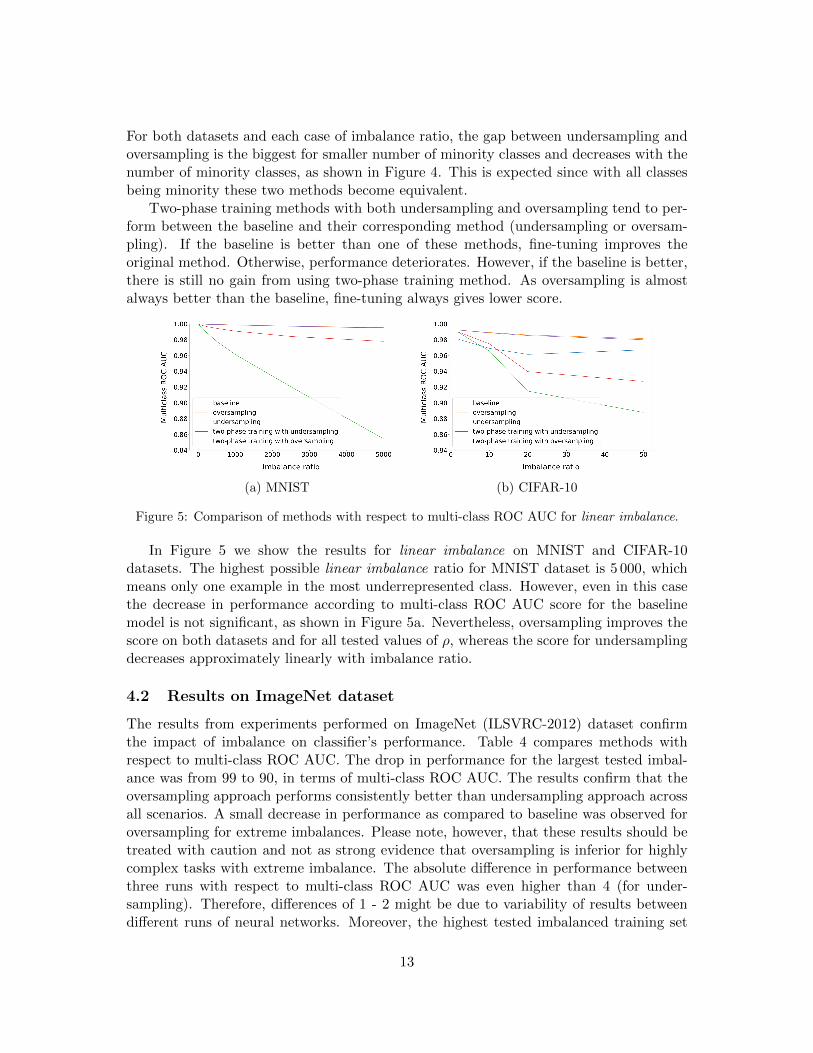
Figure 5: Comparison of methods with respect to multi-class ROC AUC for linear imbalance.

In Figure 5 we show the results for linear imbalance on MNIST and CIFAR-10datasets. The highest possible linear imbalance ratio for MNIST dataset is 5 000, whichmeans only one example in the most underrepresented class. However, even in this casethe decrease in performance according to multi-class ROC AUC score for the baselinemodel is not significant, as shown in Figure 5a. Nevertheless, oversampling improves thescore on both datasets and for all tested values of ρ, whereas the score for undersamplingdecreases approximately linearly with imbalance ratio.

4.2 Results on ImageNet dataset

The results from experiments performed on ImageNet (ILSVRC-2012) dataset confirmthe impact of imbalance on classifier’s performance. Table 4 compares methods withrespect to multi-class ROC AUC. The drop in performance for the largest tested imbal-ance was from 99 to 90, in terms of multi-class ROC AUC. The results confirm that theoversampling approach performs consistently better than undersampling approach acrossall scenarios. A small decrease in performance as compared to baseline was observed foroversampling for extreme imbalances. Please note, however, that these results should betreated with caution and not as strong evidence that oversampling is inferior for highlycomplex tasks with extreme imbalance. The absolute difference in performance betweenthree runs with respect to multi-class ROC AUC was even higher than 4 (for under-sampling). Therefore, differences of 1 - 2 might be due to variability of results betweendifferent runs of neural networks. Moreover, the highest tested imbalanced training set

13

was only about 10% of the original ILSVRC-2012 introducing confounding issues such asthe optimal training hyperparameters for this significantly changed dataset. Therefore,while these results indicate that caution should be taken when any sampling techniqueis applied to highly complex tasks with extreme imbalances, it needs a more extensivestudy devoted to this specific issue.

Method µ = 0.1, ρ = 10 µ = 0.8, ρ = 50 µ = 0.9, ρ = 100

Baseline 99.41 96.31 90.74 90.46 90.05Oversampling 99.35 95.06 88.38 88.39 88.17

Undersampling 96.85 94.98 88.35 84.08 83.74

Table 4: Comparison of results on ImageNet with respect to multi-class ROC AUC.

4.3 Separation of effects from reduced number of examples and classimbalance

An important question that needs to be considered in the context of our study is whetherthe decrease in performance for imbalanced datasets is merely caused by the fact thatour imbalanced datasets simply had fewer training examples or is it truly caused by thefact that the datasets are imbalanced.

First, we notice that oversampling method uses the same amount of data as thebaseline. It only eliminates the imbalance which is enough to improve the performancein almost all the cases. Still, it does not reach the performance of a classifier trained onthe original dataset. This is an indication that the effect of imbalance is not trivial.

Second, for some cases undersampling, which reduces the total number of cases per-forms better than the baseline (see Figures 3c and 3f). Moreover, there are even caseswhen undersampling can perform on a par with oversampling. It means that, between twosampling methods that eliminate imbalance, even using fewer data can be comparable.

In addition, for the same value of parameter ρ we have equal number of examples inthe training set for linear imbalance and step imbalance with µ = 0.5, which correspondsto half of the classes being minority. The drop in performance is much higher for stepimbalance. This additionally demonstrates that not only the total number of examplesmatters but also its distribution between classes.

4.4 Improving accuracy score with multi-class thresholding

While our focus is on ROC AUC, we also provide the evaluation of the methods based onoverall accuracy measure with results on step imbalance shown in Figure 6. As explainedin Section 3.4, accuracy has some known limitations and in some scenarios does not reflectthe discriminative power of a classifier but rather the prevalence of classes in the trainingor test set. Nevertheless, it is still commonly used evaluation score [16] and therefore weprovide some results according to this metric.

Our results show that thresholding is an appropriate approach to take to offset theprior probabilities of different classes learned by a network based on imbalanced datasets

14

and provided an improvement in overall accuracy. In general, thresholding worked par-ticularly well when applied jointly with oversampling.

(a) 2 minority classes (b) 5 minority classes (c) 8 minority classes

(d) 2 minority classes (e) 5 minority classes (f) 8 minority classes

Figure 6: Comparison of methods with respect to accuracy on MNIST (a - c) and CIFAR-10(d - f) for step imbalance with fixed number of minority classes.

Please note that thresholding does not have an actual effect on the ability of theclassifier to discriminate between a given class from another but rather helps to find athreshold on the network output that guarantees a large number of correctly classifiedcases. In terms of ROC, multiplying a decision variable by any positive number does notchange the area under the ROC curve. However, finding an optimal operating point onthe ROC curve is important when the overall number of correctly classified cases is ofinterest.

4.5 Undersampling and oversampling to smaller imbalance ratio

The default version of oversampling is to increase the number of cases in the minorityclasses so that the number matches the majority classes. Similarly, the default of under-sampling is to decrease the number of cases in the majority classes to match the minorityclasses. However, a more moderate version of these algorithms could be applied. Forthe case of MNIST with imbalance ratio of 1 000 we have tried to gradually decrease theimbalance with oversampling and undersampling. The results are shown in Figure 7.

The results show that the default version of oversampling was always the best. Anyreduction of imbalance improves the score regardless of the number of minority classes,

15

as shown in Figure 7a. For undersampling, in some cases of moderate number of minorityclasses, intermediate levels of undersampling performed better than both full undersam-pling and the baseline.

(a) Oversampling (b) Undersampling

Figure 7: Comparison of oversampling and undersampling to reduced imbalance ratios on MNISTwith original imbalance of 1 000.

Moreover, comparing undersampling and oversampling to reduced level of imbalance,we can notice that for each case of oversampling there is a level to which we can applyundersampling and achieve equivalent performance. However, that level is not known apriori rendering oversampling still the method of choice.

4.6 Generalization of sampling methods

In some cases undersampling and oversampling perform similarly. In those cases, onewould probably prefer the model that generalizes better. For classical machine learningmodels it was shown that oversampling can cause overfitting, especially for minorityclasses [33]. As we repeat small number of examples multiple times, the trained modelfits them too well. Thus, according to this prior knowledge undersampling would bea better choice. The results from our experiments do not confirm this conclusion forconvolutional neural networks.

(a) Baseline (b) Oversampling (c) Undersampling

Figure 8: Comparison of networks convergence between baseline and sampling methods. Trainingon CIFAR-10 step imbalanced with 5 minority classes and imbalance ratio of 50.

16

In Figure 8 we compare the convergence of baseline and sampling methods for CI-FAR-10 experiments with respect to accuracy. Both methods helped to train a betterclassifier in terms of performance and generalization. They also made training more sta-ble. However, in this case it is not true that oversampling leads to overfitting. Accuracydoes not decrease as the training progresses and the gap between accuracy on the trainingand test sets is smaller for oversampling, Figure 8b, than undersampling, Figure 8c. Thisobservation also holds for MNIST and ImageNet datasets and other cases of imbalance.

5 Conclusions

In this study, we examined the impact of class imbalance on classification performanceof convolutional neural networks and investigated the effectiveness of different methodsof addressing the issue. We defined and parametrized two representative types of im-balance, i.e. step and linear. Then we subsampled MNIST, CIFAR-10 and ImageNet(ILSVRC-2012) datasets to make them artificially imbalanced. We have compared com-mon sampling methods, basic thresholding, and two-phase training.

The conclusions from our experiments related to the class imbalance are as follows.

• The effect of class imbalance on classification performance is detrimental.

• The influence of imbalance on classification performance increases with the scale ofa task.

• The impact of imbalance cannot be explained simply by the lower total number oftraining cases and depends on the distribution of examples among classes.

Regarding the choice of a method to handle CNN training on imbalanced dataset weconclude the following.

• The method that in most of the cases outperforms all others with respect to multi-class ROC AUC was oversampling.

• For extreme ratio of imbalance and large portion of classes being minority, under-sampling performs on a par with oversampling.

• To achieve the best accuracy, one should apply thresholding to compensate for priorclass probabilities. A combination of thresholding with baseline and oversamplingis the most preferable, whereas it should not be combined with undersampling.

• Oversampling should be applied to the level that totally eliminates the imbalance,whereas undersampling can perform better when the imbalance is only removed tosome extent.

• As opposed to some classical machine learning models, oversampling does not nec-essarily cause overfitting of convolutional neural networks.

17

References

[1] Jiuxiang Gu, Zhenhua Wang, Jason Kuen, Lianyang Ma, Amir Shahroudy, BingShuai, Ting Liu, Xingxing Wang, and Gang Wang. Recent advances in convolutionalneural networks. arXiv preprint arXiv:1512.07108, 2015.

[2] Matthew D Zeiler and Rob Fergus. Visualizing and understanding convolutionalnetworks. In European conference on computer vision, pages 818–833. Springer,2014.

[3] Yann LeCun, Bernhard Boser, John S Denker, Donnie Henderson, Richard E Howard,Wayne Hubbard, and Lawrence D Jackel. Backpropagation applied to handwrittenzip code recognition. Neural computation, 1(4):541–551, 1989.

[4] Alex Krizhevsky, Ilya Sutskever, and Geoffrey E Hinton. Imagenet classification withdeep convolutional neural networks. In Advances in neural information processingsystems, pages 1097–1105, 2012.

[5] Karen Simonyan and Andrew Zisserman. Very deep convolutional networks for large-scale image recognition. arXiv preprint arXiv:1409.1556, 2014.

[6] Grant Van Horn, Oisin Mac Aodha, Yang Song, Alex Shepard, Hartwig Adam, PietroPerona, and Serge Belongie. The inaturalist challenge 2017 dataset. arXiv preprintarXiv:1707.06642, 2017.

[7] Jianxiong Xiao, James Hays, Krista A Ehinger, Aude Oliva, and Antonio Torralba.Sun database: Large-scale scene recognition from abbey to zoo. In Computer visionand pattern recognition (CVPR), 2010 IEEE conference on, pages 3485–3492. IEEE,2010.

[8] Brian Alan Johnson, Ryutaro Tateishi, and Nguyen Thanh Hoan. A hybrid pansharp-ening approach and multiscale object-based image analysis for mapping diseased pineand oak trees. International journal of remote sensing, 34(20):6969–6982, 2013.

[9] Miroslav Kubat, Robert C Holte, and Stan Matwin. Machine learning for the de-tection of oil spills in satellite radar images. Machine learning, 30(2-3):195–215,1998.

[10] Oscar Beijbom, Peter J Edmunds, David I Kline, B Greg Mitchell, and David Krieg-man. Automated annotation of coral reef survey images. In Computer Vision andPattern Recognition (CVPR), 2012 IEEE Conference on, pages 1170–1177. IEEE,2012.

[11] Jerzy W Grzymala-Busse, Linda K Goodwin, Witold J Grzymala-Busse, and XinqunZheng. An approach to imbalanced data sets based on changing rule strength. InRough-Neural Computing, pages 543–553. Springer, 2004.

18

[12] Brian Mac Namee, Padraig Cunningham, Stephen Byrne, and Owen I Corrigan. Theproblem of bias in training data in regression problems in medical decision support.Artificial intelligence in medicine, 24(1):51–70, 2002.

[13] Philip K Chan and Salvatore J Stolfo. Toward scalable learning with non-uniformclass and cost distributions: A case study in credit card fraud detection. In KDD,volume 1998, pages 164–168, 1998.

[14] Predrag Radivojac, Nitesh V Chawla, A Keith Dunker, and Zoran Obradovic. Clas-sification and knowledge discovery in protein databases. Journal of Biomedical In-formatics, 37(4):224–239, 2004.

[15] Claire Cardie and Nicholas Howe. Improving minority class prediction using case-specific feature weights. In ICML, pages 57–65, 1997.

[16] Guo Haixiang, Li Yijing, Jennifer Shang, Gu Mingyun, Huang Yuanyue, and GongBing. Learning from class-imbalanced data: Review of methods and applications.Expert Systems with Applications, 2016.

[17] Nathalie Japkowicz and Shaju Stephen. The class imbalance problem: A systematicstudy. Intelligent data analysis, 6(5):429–449, 2002.

[18] Maciej A Mazurowski, Piotr A Habas, Jacek M Zurada, Joseph Y Lo, Jay A Baker,and Georgia D Tourassi. Training neural network classifiers for medical decisionmaking: The effects of imbalanced datasets on classification performance. Neuralnetworks, 21(2):427–436, 2008.

[19] Nitesh V Chawla. Data mining for imbalanced datasets: An overview. In Datamining and knowledge discovery handbook, pages 853–867. Springer, 2005.

[20] Marcus A Maloof. Learning when data sets are imbalanced and when costs areunequal and unknown. In ICML-2003 workshop on learning from imbalanced datasets II, volume 2, pages 2–1, 2003.

[21] Charles X Ling and Chenghui Li. Data mining for direct marketing: Problems andsolutions. In KDD, volume 98, pages 73–79, 1998.

[22] Zhi-Hua Zhou and Xu-Ying Liu. Training cost-sensitive neural networks with meth-ods addressing the class imbalance problem. IEEE Transactions on Knowledge andData Engineering, 18(1):63–77, 2006.

[23] Steve Lawrence, Ian Burns, Andrew Back, Ah Chung Tsoi, and C Lee Giles. Neuralnetwork classification and prior class probabilities. In Neural networks: tricks of thetrade, pages 299–313. Springer, 1998.

[24] Salman H Khan, Mohammed Bennamoun, Ferdous Sohel, and Roberto Togneri.Cost sensitive learning of deep feature representations from imbalanced data. arXivpreprint arXiv:1508.03422, 2015.

19

[25] Vidwath Raj, Sven Magg, and Stefan Wermter. Towards effective classification ofimbalanced data with convolutional neural networks. In IAPR Workshop on ArtificialNeural Networks in Pattern Recognition, pages 150–162. Springer, 2016.

[26] Yu-An Chung, Hsuan-Tien Lin, and Shao-Wen Yang. Cost-aware pre-training formulticlass cost-sensitive deep learning. arXiv preprint arXiv:1511.09337, 2015.

[27] Shoujin Wang, Wei Liu, Jia Wu, Longbing Cao, Qinxue Meng, and Paul J Kennedy.Training deep neural networks on imbalanced data sets. In Neural Networks(IJCNN), 2016 International Joint Conference on, pages 4368–4374. IEEE, 2016.

[28] Mohammad Havaei, Axel Davy, David Warde-Farley, Antoine Biard, AaronCourville, Yoshua Bengio, Chris Pal, Pierre-Marc Jodoin, and Hugo Larochelle. Braintumor segmentation with deep neural networks. Medical image analysis, 35:18–31,2017.

[29] Haibo He and Edwardo A Garcia. Learning from imbalanced data. IEEE Transac-tions on knowledge and data engineering, 21(9):1263–1284, 2009.

[30] Gil Levi and Tal Hassner. Age and gender classification using convolutional neuralnetworks. In Proceedings of the IEEE Conference on Computer Vision and PatternRecognition Workshops, pages 34–42, 2015.

[31] Andrew Janowczyk and Anant Madabhushi. Deep learning for digital pathology im-age analysis: A comprehensive tutorial with selected use cases. Journal of pathologyinformatics, 7, 2016.

[32] Nicolas Jaccard, Thomas W Rogers, Edward J Morton, and Lewis D Griffin. Detec-tion of concealed cars in complex cargo x-ray imagery using deep learning. Journalof X-Ray Science and Technology, pages 1–17, 2016.

[33] Nitesh V Chawla, Kevin W Bowyer, Lawrence O Hall, and W Philip Kegelmeyer.Smote: synthetic minority over-sampling technique. Journal of artificial intelligenceresearch, 16:321–357, 2002.

[34] Kung-Jeng Wang, Bunjira Makond, Kun-Huang Chen, and Kung-Min Wang. Ahybrid classifier combining smote with pso to estimate 5-year survivability of breastcancer patients. Applied Soft Computing, 20:15–24, 2014.

[35] Hui Han, Wen-Yuan Wang, and Bing-Huan Mao. Borderline-smote: a new over-sampling method in imbalanced data sets learning. Advances in intelligent computing,pages 878–887, 2005.

[36] Taeho Jo and Nathalie Japkowicz. Class imbalances versus small disjuncts. ACMSigkdd Explorations Newsletter, 6(1):40–49, 2004.

[37] Hongyu Guo and Herna L Viktor. Learning from imbalanced data sets with boost-ing and data generation: the databoost-im approach. ACM Sigkdd ExplorationsNewsletter, 6(1):30–39, 2004.

20

[38] Li Shen, Zhouchen Lin, and Qingming Huang. Relay backpropagation for effectivelearning of deep convolutional neural networks. In European Conference on ComputerVision, pages 467–482. Springer, 2016.

[39] Chris Drummond, Robert C Holte, et al. C4.5, class imbalance, and cost sensitivity:why under-sampling beats over-sampling. In Workshop on learning from imbalanceddatasets II, volume 11, pages 1–8, 2003.

[40] Miroslav Kubat, Stan Matwin, et al. Addressing the curse of imbalanced trainingsets: one-sided selection. In ICML, volume 97, pages 179–186. Nashville, USA, 1997.

[41] Jack Koplowitz and Thomas A Brown. On the relation of performance to editing innearest neighbor rules. Pattern Recognition, 13(3):251–255, 1981.

[42] Ricardo Barandela, E Rangel, Jose Salvador Sanchez, and Francesc J Ferri. Re-stricted decontamination for the imbalanced training sample problem. In Iberoamer-ican Congress on Pattern Recognition, pages 424–431. Springer, 2003.

[43] Michael D Richard and Richard P Lippmann. Neural network classifiers estimatebayesian a posteriori probabilities. Neural computation, 3(4):461–483, 1991.

[44] Charles Elkan. The foundations of cost-sensitive learning. In International jointconference on artificial intelligence, volume 17, pages 973–978. Lawrence ErlbaumAssociates Ltd, 2001.

[45] Matjaz Kukar, Igor Kononenko, et al. Cost-sensitive learning with neural networks.In ECAI, pages 445–449, 1998.

[46] Nathalie Japkowicz, Catherine Myers, Mark Gluck, et al. A novelty detection ap-proach to classification. In IJCAI, volume 1, pages 518–523, 1995.

[47] Nathalie Japkowicz, Stephen Jose Hanson, and Mark A Gluck. Nonlinear autoasso-ciation is not equivalent to pca. Neural computation, 12(3):531–545, 2000.

[48] Hoon Sohn, Keith Worden, and Charles R Farrar. Novelty detection using auto-associative neural network. In Symposium on Identification of Mechanical Systems:international mechanical engineering congress and exposition, New York, NY, pages573–580, 2001.

[49] Hyoung-joo Lee and Sungzoon Cho. The novelty detection approach for differentdegrees of class imbalance. In Neural Information Processing, pages 21–30. Springer,2006.

[50] Xu-Ying Liu, Jianxin Wu, and Zhi-Hua Zhou. Exploratory undersampling for class-imbalance learning. IEEE Transactions on Systems, Man, and Cybernetics, Part B(Cybernetics), 39(2):539–550, 2009.

21

[51] Nitesh V Chawla, Aleksandar Lazarevic, Lawrence O Hall, and Kevin W Bowyer.Smoteboost: Improving prediction of the minority class in boosting. In EuropeanConference on Principles of Data Mining and Knowledge Discovery, pages 107–119.Springer, 2003.

[52] Yann LeCun, Leon Bottou, Yoshua Bengio, and Patrick Haffner. Gradient-basedlearning applied to document recognition. Proceedings of the IEEE, 1998.

[53] Alex Krizhevsky and Geoffrey Hinton. Learning multiple layers of features from tinyimages. 2009.

[54] Olga Russakovsky, Jia Deng, Hao Su, Jonathan Krause, Sanjeev Satheesh, Sean Ma,Zhiheng Huang, Andrej Karpathy, Aditya Khosla, Michael Bernstein, et al. Imagenetlarge scale visual recognition challenge. International Journal of Computer Vision,115(3):211–252, 2015.

[55] Yangqing Jia, Evan Shelhamer, Jeff Donahue, Sergey Karayev, Jonathan Long, RossGirshick, Sergio Guadarrama, and Trevor Darrell. Caffe: Convolutional architecturefor fast feature embedding. In Proceedings of the 22nd ACM international conferenceon Multimedia, pages 675–678. ACM, 2014.

[56] Ning Qian. On the momentum term in gradient descent learning algorithms. Neuralnetworks, 12(1):145–151, 1999.

[57] Xavier Glorot and Yoshua Bengio. Understanding the difficulty of training deepfeedforward neural networks. In Aistats, volume 9, pages 249–256, 2010.

[58] Ian J Goodfellow, David Warde-Farley, Mehdi Mirza, Aaron C Courville, and YoshuaBengio. Maxout networks. ICML (3), 28:1319–1327, 2013.

[59] Jost Tobias Springenberg, Alexey Dosovitskiy, Thomas Brox, and Martin Riedmiller.Striving for simplicity: The all convolutional net. arXiv preprint arXiv:1412.6806,2014.

[60] Marcel Simon, Erik Rodner, and Joachim Denzler. Imagenet pre-trained models withbatch normalization. arXiv preprint arXiv:1612.01452, 2016.

[61] Kaiming He, Xiangyu Zhang, Shaoqing Ren, and Jian Sun. Deep residual learningfor image recognition. In Proceedings of the IEEE Conference on Computer Visionand Pattern Recognition, pages 770–778, 2016.

[62] Sergey Ioffe and Christian Szegedy. Batch normalization: Accelerating deep networktraining by reducing internal covariate shift. arXiv preprint arXiv:1502.03167, 2015.

[63] Kaiming He, Xiangyu Zhang, Shaoqing Ren, and Jian Sun. Delving deep into recti-fiers: Surpassing human-level performance on imagenet classification. In Proceedingsof the IEEE international conference on computer vision, pages 1026–1034, 2015.

22

[64] Andrew P Bradley. The use of the area under the roc curve in the evaluation ofmachine learning algorithms. Pattern recognition, 30(7):1145–1159, 1997.

[65] Charles X Ling, Jin Huang, and Harry Zhang. Auc: a statistically consistent andmore discriminating measure than accuracy. In IJCAI, volume 3, pages 519–524,2003.

[66] Foster Provost and Pedro Domingos. Tree induction for probability-based ranking.Machine learning, 52(3):199–215, 2003.

23