ANNALS OF ECONOMICS AND FINANCE 14-1, 121–144 (2013)

Inflation and Economic Growth*

Robert J. Barro

Department of Economics Littauer Center 120 Harvard University Cambridge, MA02138 and NBER

Data for around 100 countries from 1960 to 1990 are used to assess theeffects of inflation on economic performance. If a number of country char-acteristics are held constant, then regression results indicate that the impacteffects from an increase in average inflation by 10 percentage points per yearare a reduction of the growth rate of real per capita GDP by 0.2-0.3 percentagepoints per year and a decrease in the ratio of investment to GDP by 0.4-0.6percentage points. Since the statistical procedures use plausible instrumentsfor inflation, there is some reason to believe that these relations reflect causalinfluences from inflation to growth and investment. However, statistically sig-nificant results emerge only when high-inflation experiences are included inthe sample. Although the adverse influence of inflation on growth looks small,the long-term effects on standards of living are substantial. For example, ashift in monetary policy that raises the long-term average inflation rate by 10percentage points per year is estimated to lower the level of real GDP after 30years by 4-7%, more than enough to justify a strong interest in price stability.

Key Words:JEL Classification Numbers:

1. INTRODUCTION

In recent years, many central banks have placed increased emphasis onprice stability. Monetary policy-whether expressed in terms of interest ratesor growth of monetary aggregates-has been increasingly geared toward theachievement of low and stable inflation. Central bankers and most otherobservers view price stability as a worthy objective because they thinkthat inflation is costly. Some of these costs involve the average rate of in-

* The initial version of This paper was written while I was Houblon-Norman researchfellow at the Bank of England. This research was supported by the National ScienceFoundation. This paper is part of NBER’s research programs in Economic Fluctuations,Growth, and Monetary Economics. Any opinions expressed are those of the author andnot those of the National Bureau of Economic Research.

121

1529-7373/2013All rights of reproduction in any form reserved.

122 ROBERT J. BARRO

flation and others relate to the variability and uncertainty of inflation. Butthe general idea is that businesses and households are thought to performpoorly when inflation is high and unpredictable.

The academic literature contains a lot of theoretical work on the costs ofinflation, as reviewed recently by Briault (1995). This analysis provides apresumption that inflation is a bad idea, but the case is not decisive with-out supporting empirical findings. Although some empirical results (alsosurveyed by Briault) suggest that inflation is harmful, the evidence is notoverwhelming. It is therefore important to carry out additional empiricalresearch on the relation between inflation and economic performance. Thispaper explores this relation in a large sample of countries over the last 30years.

2. DATA

The data set covers over 100 countries from 1960 to 1990. Table 1 pro-vides information about the behavior of inflation in this sample. Annualinflation rates were computed in most cases from consumer price indexes.(The deflator for the gross domestic product was used in a few instances,when the data on consumer prices were unavailable.) The table showsthe mean and median across the countries of the inflation rates in threedecades: 1960-70, 1970-80, and 1980-90. The median inflation rate was3.3% per year in the 1960s (117 countries), 10.1% in the 1970s (122 coun-tries), and 8.9% in the 1980s (119 countries). The upper panel of Figure 1provides a histogram for the inflation rates observed over the three decades.The bottom panel applies to the 44 observations for which the inflation rateexceeded 20% per year.1

The annual data were used for each country over each decade to computea measure of inflation variability, the standard deviation of the inflationrate around its decadal mean. Table 1 shows the mean and median ofthese standard deviations for the three decades. The median was 2.4% peryear in the 1960s, 5.4% in the 1970s, and 4.9% in the 1980s. Thus, a rise ininflation variability accompanied the increase in the average inflation ratesince the 1960s.

Figure 2 confirms the well-known view that a higher variability of infla-tion tends to accompany a higher average rate of inflation (see, for example,Okun [1971] and Logue and Willett [1976]). These charts provide scatter

1Table 1 shows that the cross-country mean of inflation exceeded the median for eachdecade. This property reflects the skewing of inflation rates to the right, as shownin Figure 1. That is, there are a number of outliers with positive inflation rates oflarge magnitude, but none with negative inflation rates of high magnitude Because Thisskewness increased in the 1980s, the mean inflation rate rose from the 1970s to the 1980s,although the median rate declined.

INFLATION AND ECONOMIC GROWTH 123

FIG. 1. Histograms for Inflation Rate

Ii

I

a

I

TUtJVtTOU L$Ø (toi. siyrzes vpos. so bn len)

FJflLG I flT2fOL9W2 LOL Iuuscrou Bf

WtIflTOU LV(S

oeo 080

Ii

I

a

I

TUtJVtTOU L$Ø (toi. siyrzes vpos. so bn len)

FJflLG I flT2fOL9W2 LOL Iuuscrou Bf

WtIflTOU LV(S

oeo 080

plots for each decade of the standard deviation of inflation (measured foreach country around its own decadal mean) against the average inflationrate (the mean of each country’s inflation rate over the decade). The upperpanel considers only inflation rates below 15% per year, the middle panelincludes values above 15% per year, and the lower panel covers the entirerange. The positive, but imperfect, relation between variability and meanis apparent throughout.

124 ROBERT J. BARRO

TABLE 1.

Descriptive Statistics on Inflation, Growth, and Investment

Variable Mean Median Number of Countries

1960-70:

inflation rate 0.054 0.033 117

standard deviation of inflation rate 0.039 0.024 117

growth rate of real per capita GDP 0.028 0.031 118

ratio of investment to GDP 0.168 0.156 119

1970-80:

inflation rate 0.133 0.101 122

standard deviation of inflation rate 0.075 0.054 122

growth rate of real per capita GDP 0.023 0.025 123

ratio of investment to GDP 0.191 0.193 123

1980-90:

inflation rate 0.191 0.089 119

standard deviation of inflation rate 0.134 0.049 119

growth rate of real per capita GDP 0.003 0.004 121

ratio of investment to GDP 0.174 0.173 128

Notes: The inflation rate is computed on an annual basis for each country from dataon consumer price indexes from the World Bank, STARS databank and issues of WorldTables; International Monetary Fund, International financial Statistics, yearbook issues;and individual country sources). In a few cases, figures on the GDP deflator were used.The average inflation rate for each country in each decade is the mean of the annualrates. The standard deviation for each country in each decade is the square root ofthe squared difference of the annual inflation rate from the decadal mean. The valuesshown for inflation in This table are the mean or median across the countries of thedecade-average inflation rates. Similarly, the figures for standard deviations are themean or median across the countries of the standard deviations for each decade. Thegrowth rates of real per capita GDP are based on the purchasing-power adjusted GDPvalues compiled by Summers and Heston (1993). For the 1985-90 period, some of thefigures come from the World Bank (and are based on market exchange rates ratherthan purchasingpower comparisons). The ratios of real investment (private plus public)to real GDP come from Summers and Heston (1993). These values are averages for1960-69, 1970-79, and 1980-89.

Table 1 also gives the means and medians of the growth rate of realper capita GDP and the ratio of investment to GDP for the three decades.The median growth rate fell from 3.1% in the 1960s (118 countries) to 2.5%in the 1970s (123 countries) and 0.4% in the 1980s (121 countries). Themedian investment ratio went from 16% in the 1960s to 19% in the 1970sand 17% in the 1980s. In contrast to inflation rates, the growth rates andinvestment ratios tend to be symmetrically distributed around the median.

INFLATION AND ECONOMIC GROWTH 125

FIG. 2. Standard Deviation of Inflation Versus Mean Inflation

I

II

II

Im

II

II

I

2

I

&,O2

LI A*u i b.

00

IPUVV L AII b. ).w)

IULIrOU AGL2( yGU iUçrou

E1I1LG S DGAcIOU O

I

II

II

Im

II

II

I

2

I

&,O2

LI A*u i b.

00

IPUVV L AII b. ).w)

IULIrOU AGL2( yGU iUçrou

E1I1LG S DGAcIOU O

I

II

II

Im

II

II

I

2

I

&,O2

LI A*u i b.

00

IPUVV L AII b. ).w)

IULIrOU AGL2( yGU iUçrou

E1I1LG S DGAcIOU O

3. FRAMEWORK FOR THE ANALYSIS OF GROWTH

To assess the effect of inflation on economic growth, I use a system ofregression equations in which many other determinants of growth are heldconstant. The framework is based on an extended view of the neoclassicalgrowth model, as described in Barro and Sala-i-Martin (1995, Chs. 1,2).My empirical implementations of this approach include Barro (1991, 1996).

A general notion in the framework is that an array of government policiesand private-sector choices determine where an economy will go in the longrun. For example, favorable public policies—including better maintenanceof the rule of law and property rights, fewer distortions of private markets,less nonproductive government consumption, and greater public investmentin high-return areas—lead in the long run to higher levels of real per capitaGDP. (Henceforth, the term GDP will be used as a shorthand to denotereal per capita GDP.) Similarly, a greater willingness of the private sectorto save and a reduced tendency to expend resources on child rearing (lowerfertility and population growth) tend to raise standards of living in thelong run.

Given the determinants of the long-run position, an economy tends cur-rently to grow faster the lower its GDP. In other words, an economy’s per

126 ROBERT J. BARRO

capita growth rate is increasing in the gap between its long-term prospec-tive GDP and its current GDP. This force generates a convergence tendencyin which poor countries grow faster than rich countries and tend therebyto catch up in a proportional sense to the rich places. However, poor coun-tries grow fast only if they have favorable settings for government policiesand private-sector choices. If a poor country selects unfavorable policies—a choice that likely explains why the country is currently observed to bepoor-then its growth rate will not be high and it will not tend to catch upto the richer places.

Another important element is a country’s human capital in the forms ofeducation and health. For given values of prospective and actual GDP,a country grows faster—that is, approaches its long-run position morerapidly—the greater its current level of human capital. This effect arisesbecause, first, physical capital tends to expand rapidly to match a highendowment of human capital, and, second, a country with more humancapital is better equipped to acquire and adapt the efficient technologiesthat have been developed in the leading countries.

4. PANEL ESTIMATES OF GROWTH EQUATIONS

4.1. Overview of the Results

Table 2 lists the explanatory variables used as determinants of the growthrate of real per capita GDP. The details for a similar setup are in Barro(1996). The results apply to growth rates and the other variables observedfor 78 countries from 1965 to 1975, 89 countries for 1975 to 1985, and 84countries from 1985 to 1990. This sample reflects the availability of thenecessary data. The first period starts in 1965, rather than 1960, so that5-year lags of the explanatory variables are available.

The estimation is by instrumental variables, where the instruments con-sist mainly of prior values of the regressors. For example, the 1965-75equation includes the log of 1965 GDP on the right-hand side and usesthe log of 1960 GDP as an instrument. This procedure should lessen theestimation problems caused by temporary measurement error in GDP. Theright-hand side also contains period averages of several variables — govern-ment spending ratios, fertility rates, black-market premia, and investmentratios — and uses 5-year earlier values of these variables as instruments.

The use of lagged variables as instruments is problematic, although bet-ter alternatives are not obvious. One favorable element here is that theresiduals from the growth equations turn out to be virtually uncorrelatedover the time periods. In most respects, the instrumental results do notdiffer greatly from OLS estimates. The largest difference turns out to befor the estimated effect of the investment ratio on the growth rate.

INFLATION AND ECONOMIC GROWTH 127

TABLE 2.

Regressions for Per Capita Growth Rate

Variable (1) (2) (3) (4) (5)

log(GDP) −0.0241 −0.0242 −0.0246 −0.0242 −0.0231

(0.0030) (0.0030) (0.0029) (0.0030) (0.0029)

male 0.0144 0.0145 0.0146 0.0136 0.0116

schooling (0.0036) (0.0036) (0.0036) (0.0037) (0.0038)

female −0.0100 −0.0100 −0.0104 −0.0087 −0.0063

schooling (0.0049) (0.0049) (0.0050) (0.0052) (0.0053)

log(life 0.0359 0.0354 0.0381 0.0333 0.0407

expectancy) (0.0122) (0.0121) (0.0124) (0.0120) (0.0130)

log(GDP)*human −0.44 −0.44 −0.41 −0.47 −0.45

capital (0.17) (0.17) (0.17) (0.17) (0.16)

log(fertility −0.0175 −0.0175 −0.0173 −0.0176 −0.0146

rate) (0.0053) (0.0053) (0.0053) (0.0053) (0.0055)

govt. consump −0.117 −0.116 −0.118 −0.120 −0.115

ratio (0.027) (0.027) (0.027) (0.027) (0.026)

public educ. 0.114 0.112 0.146 0.081 0.057

spending ratio (0.090) (0.089) (0.090) (0.091) (0.091)

black-market −0.0127 −0.0125 −0.0150 −0.0109 −0.0137

premium (0.0052) (0.0051) (0.0050) (0.0055) (0.0054)

rule-of-law 0.00426 0.00424 0.00426 0.00418 0.00404

index (0.00093) (0.00093) (0.00093) (0.00095) (0.00093)

terms-of-trade 0.126 0.127 0.129 0.123 0.117

change (0.028) (0.028) (0.028) (0.028) (0.028)

investment 0.019 0.020 0.018 0.024 0.013

ratio (0.022) (0.022) (0.022) (0.022) (0.022)

democ. index −0.064 −0.063 −0.067 −0.060 −0.066

squared (0.022) (0.022) (0.023) (0.023) (0.023)

inflation −0.0236 −0.0209 −0.0197 −0.0306 −0.0254

rate (0.0048) (0.0082) (0.0069) (0.0083) (0.0086)

Since the general pattern of results has been considered elsewhere (forexample, Barro[1996]), I will provide only a brief sketch here and will fo-cus the main discussion on the effects of inflation. One familiar findingin Table 2 is that the estimated coefficient on initial log(GDP ) is signifi-cantly negative with a magnitude of around 2.5%. Thus, conditional on theother variables, convergence in real per capita GDP occurs at roughly 2.5%per year.2 Growth tends also to be increasing in the initial levels of hu-

2The actual rate is slightly higher because the observed growth rates are averages overperiods of 10 or 5 years. See Barro and Sala-i-Martin(1995, p. 81)

128 ROBERT J. BARRO

TABLE 2—Continued

Variable (1) (2) (3) (4) (5)

democracy 0.063 0.063 0.066 0.059 0.066

index (0.025) (0.025) (0.025) (0.026) (0.026)

stnd. dev. of −0.0036

inflation rate (0.0086)

Latin Amer. −0.0060

dummy (0.0034)

R2 0.63, 0.60, 0.63, 0.60, 0.64, 0.60, 0.63, 0.59, 0.63, 0.61,

0.48 0.49 0.46 0.48 0.49

number of 78, 89, 78, 89, 78, 89, 78, 89, 78, 89,

observations 84 84 84 84 84

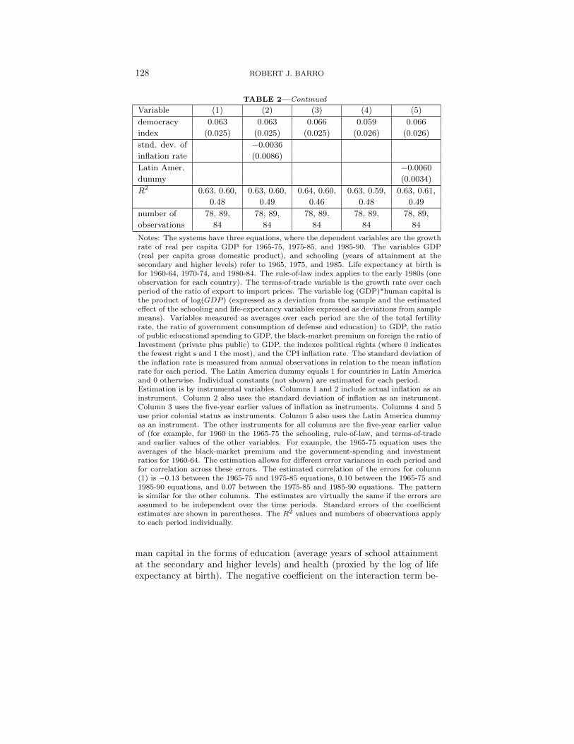
Notes: The systems have three equations, where the dependent variables are the growthrate of real per capita GDP for 1965-75, 1975-85, and 1985-90. The variables GDP(real per capita gross domestic product), and schooling (years of attainment at thesecondary and higher levels) refer to 1965, 1975, and 1985. Life expectancy at birth isfor 1960-64, 1970-74, and 1980-84. The rule-of-law index applies to the early 1980s (oneobservation for each country). The terms-of-trade variable is the growth rate over eachperiod of the ratio of export to import prices. The variable log (GDP)*human capital isthe product of log(GDP ) (expressed as a deviation from the sample and the estimatedeffect of the schooling and life-expectancy variables expressed as deviations from samplemeans). Variables measured as averages over each period are the of the total fertilityrate, the ratio of government consumption of defense and education) to GDP, the ratioof public educational spending to GDP, the black-market premium on foreign the ratio ofInvestment (private plus public) to GDP, the indexes political rights (where 0 indicatesthe fewest right s and 1 the most), and the CPI inflation rate. The standard deviation ofthe inflation rate is measured from annual observations in relation to the mean inflationrate for each period. The Latin America dummy equals 1 for countries in Latin Americaand 0 otherwise. Individual constants (not shown) are estimated for each period.Estimation is by instrumental variables. Columns 1 and 2 include actual inflation as aninstrument. Column 2 also uses the standard deviation of inflation as an instrument.Column 3 uses the five-year earlier values of inflation as instruments. Columns 4 and 5use prior colonial status as instruments. Column 5 also uses the Latin America dummyas an instrument. The other instruments for all columns are the five-year earlier valueof (for example, for 1960 in the 1965-75 the schooling, rule-of-law, and terms-of-tradeand earlier values of the other variables. For example, the 1965-75 equation uses theaverages of the black-market premium and the government-spending and investmentratios for 1960-64. The estimation allows for different error variances in each period andfor correlation across these errors. The estimated correlation of the errors for column(1) is −0.13 between the 1965-75 and 1975-85 equations, 0.10 between the 1965-75 and1985-90 equations, and 0.07 between the 1975-85 and 1985-90 equations. The patternis similar for the other columns. The estimates are virtually the same if the errors areassumed to be independent over the time periods. Standard errors of the coefficientestimates are shown in parentheses. The R2 values and numbers of observations applyto each period individually.

man capital in the forms of education (average years of school attainmentat the secondary and higher levels) and health (proxied by the log of lifeexpectancy at birth). The negative coefficient on the interaction term be-

INFLATION AND ECONOMIC GROWTH 129

tween initial GDP and human capital3 means that the rate of convergenceis higher in a place that starts with more human capital.

For given starting values of the state variables (represented by initial hu-man capital and GDP), growth is estimated to fall with higher fertility (theaverage woman’s total fertility rate), higher government consumption (theratio to GDP of government consumption exclusive of spending on educa-tion and defense), and a larger black-market premium on foreign exchange(intended as a proxy for market distortions more broadly).

Growth is enhanced by greater maintenance of the rule of law, as mea-sured by Knack and Keefer’s (1994) subjective index. One problem hereis that this variable is observed only in the early 1980s (and is includedamong the instruments). Growth also rises in response to a contempora-neous improvement in the terms of trade, measured by the growth rate ofthe ratio of export to import prices. (The contemporaneous terms-of-tradechange is included with the instruments.)

The estimated coefficients on the ratio of public educational spending toGDP and on the ratio of total real investment to real GDP are positive, butinsignificant. The estimated coefficient on investment becomes higher andsignificant if the contemporaneous investment ratio is included with theinstruments. (The timing in the data indicates that much of the positiveassociation between investment and growth represents the reverse responseof investment to growth.) The estimate becomes even larger and resemblesthat reported in other studies, such as Mankiw, Romer, and Weil (1992),if life expectancy is deleted as a regressor.

Finally, an increase in democracy—measured by indexes of political rightsfrom Gastil (1982-83) and Bollen (1990)—have a nonlinear effect (Which Idid not find for log[GDP ] or the human-capital variables). At low levels ofdemocracy, more freedom is estimated to raise growth. But once a moder-ate level of democracy is attained (corresponding roughly to “half” the waytoward full representative democracy), further liberalization is estimatedto reduce growth. These effects are discussed at length in Barro (1996).

4.2. Preliminary Results on Inflation

To get a first-pass estimate of the effect of inflation on economic growth, Iincluded the inflation rate over each period as an explanatory variable alongwith the other growth determinants listed in Table 2. If contemporaneousinflation is also included with the instruments, then column 1 of the tableindicates that the estimated coefficient of inflation is −0.024 (s.e. = 0.005).Thus, an increase by 10 percentage points in the annual inflation rate isassociated on impact with a decline by 0.24 percentage points in the annual

3Human capital is measured as the overall estimated effect from the levels of schoolattainment and the log of life expectancy.

130 ROBERT J. BARRO

growth rate of GDP. Since the “t-statistic” for the estimated coefficient is4.9, this result is statistically significant.4

Figure 3 depicts graphically the relation between growth and inflation.The horizontal axis plots the inflation rate; each observation correspondsto the average rate for a particular country over one of the time periodsconsidered (1965-75, 1975-85, and 1985-90). The top panel in the chartconsiders inflation rates below 15% per year, the middle panel includesvalues above 15% per year, and the bottom panel covers the full range ofinflation. The vertical axis plots the growth rate of GDP, net of the part ofthe growth rate that is explained by all of the explanatory variables asidefrom the inflation rate.5 Thus, the panels illustrate the relation betweengrowth and inflation after all of the other growth determinants have beenheld constant.

FIG. 3. Growth Rate (part unexplained by other variable s) and Inflation Rate

—Qi 00 10 10 Si SO

010

PUI aPT vp... b00 oo ro ro si si—010

i'uv' &. (i pv b u)—000 —000 OiQ 010 010 050____________________________________________________-

-oiOo

r •.•

• S • ••°'°°

0'OSO • • :

p? OfGL A9LrpJG2) uq uçrou B9G

LTnLG 3 CLOJ4P Jç (bLf nuGxbr9rucq

—Qi 00 10 10 Si SO

010

PUI aPT vp... b00 oo ro ro si si—010

i'uv' &. (i pv b u)—000 —000 OiQ 010 010 050____________________________________________________-

-oiOo

r •.•

• S • ••°'°°

0'OSO • • :

p? OfGL A9LrpJG2) uq uçrou B9G

LTnLG 3 CLOJ4P Jç (bLf nuGxbr9rucq

—Qi 00 10 10 Si SO

010

PUI aPT vp... b00 oo ro ro si si—010

i'uv' &. (i pv b u)—000 —000 OiQ 010 010 050____________________________________________________-

-oiOo

r •.•

• S • ••°'°°

0'OSO • • :

p? OfGL A9LrpJG2) uq uçrou B9G

LTnLG 3 CLOJ4P Jç (bLf nuGxbr9rucq

4This estimate is similar to that reported by Fischer (1993, Table 9). For earlierestimates of inflation variables in cross-country regressions, see Kormendi and Meguire(1985) and Grier and Tullock (1989).

5The residual is computed from the regression system that includes all of the variables,including the inflation rate. But the contribution from the inflation rate is left out tocompute the variable on the vertical axis in the scatter diagram. The residual has alsobeen normalized to have a zero mean.

INFLATION AND ECONOMIC GROWTH 131

The panels of Figure 3 show downward-sloping regression lines (least-squares lines) through the scatter plots. The slope of the line in the lowerpanel corresponds approximately to the significantly negative coefficientshown in column 1 of Table 2. The panels show, however, that the fit isdominated by the inverse relation between growth and inflation at highrates of inflation. For inflation rates below 15% per year, as shown in theupper panel, the relation between growth and inflation is not statisticallysignificant.

To put it another way, one can reestimate the panel while restrictingthe observations to those for Which the inflation rate is less than somecutoff value, x. To get a statistically significant estimate for the inflationcoefficient, x has to be raised to roughly 50% per year. With an infla-tion cutoff of 50%, the estimated coefficient is −0.029 (0.015). For lowervalues of the cutoff, the estimated coefficient tends to be negative but in-significant; some results are x = 40%, coeff.= −0.023 (0.018); x = 25%,coeff.= −0.011(0.027); x = 15%, coeff.= −0.032(0.042).

The results indicate that there is not enough information in the low-inflation experiences to isolate precisely the effect of inflation on growth,but do not necessarily mean that This effect is small at low rates of infla-tion. To check for linearity of the relation between growth and inflation, Ireestimated the system on the whole sample with separate coefficients forinflation in three ranges: up to 15%, between 15 and 40%, and over 40%.The estimated coefficients on inflation in this form are −0.016 (0.035) inthe low range, −0.037 (0.017) in the middle range, and −0.023 (0.005) inthe upper range. Thus, the clear evidence for the negative relation betweengrowth and inflation comes from the middle and upper intervals. However,since the three estimated coefficients do not differ significantly from eachother (p-value = 0.65), the data are consistent with a linear relationship.In particular, even at low rates of inflation, the data would not reject thehypothesis that growth is negatively related to inflation.

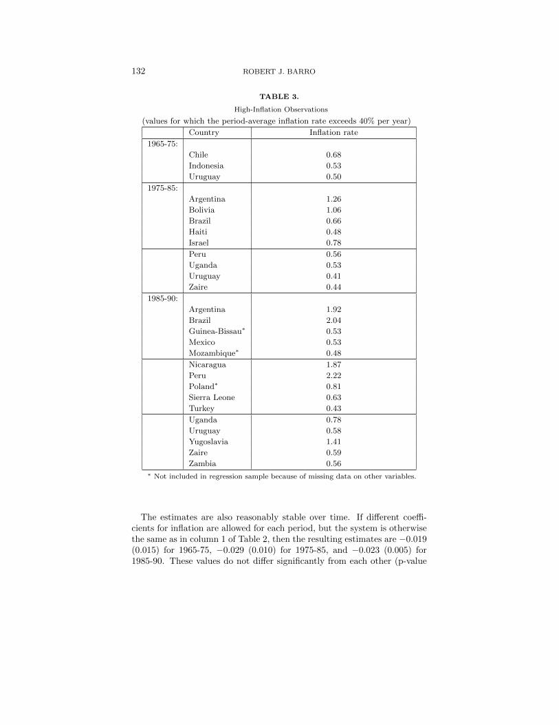
Although statistically significant effects arise only when the high-inflationexperiences are included, the results are not sensitive to a few outlier obser-vations. Table 3 shows the 27 cases of inflation in excess of 40% per yearfor one of the time periods (1965-75, 1975-85, and 1985-90). Note thatUruguay appears 3 times (although it is by no means the overall cham-pion for high inflation), and Argentina, Brazil, Peru, Uganda, and Zaireshow up twice each. The other countries, with one observation each, areChile, Indonesia, Bolivia, Haiti, Israel, Guinea-Bissau, Mexico, Mozam-bique, Nicaragua, Poland, Sierra Leone, Turkey, Yugoslavia, and Zambia.(Guinea-Bissau, Mozambique, and Poland are excluded from the regres-sion sample because of missing data on other variables.) The exclusionof any small number of these high-inflation observations—Nicaragua andZaire had been suggested to me—has a negligible effect on the results.

132 ROBERT J. BARRO

TABLE 3.

High-Inflation Observations

(values for which the period-average inflation rate exceeds 40% per year)

Country Inflation rate

1965-75:

Chile 0.68

Indonesia 0.53

Uruguay 0.50

1975-85:

Argentina 1.26

Bolivia 1.06

Brazil 0.66

Haiti 0.48

Israel 0.78

Peru 0.56

Uganda 0.53

Uruguay 0.41

Zaire 0.44

1985-90:

Argentina 1.92

Brazil 2.04

Guinea-Bissau∗ 0.53

Mexico 0.53

Mozambique∗ 0.48

Nicaragua 1.87

Peru 2.22

Poland∗ 0.81

Sierra Leone 0.63

Turkey 0.43

Uganda 0.78

Uruguay 0.58

Yugoslavia 1.41

Zaire 0.59

Zambia 0.56∗ Not included in regression sample because of missing data on other variables.

The estimates are also reasonably stable over time. If different coeffi-cients for inflation are allowed for each period, but the system is otherwisethe same as in column 1 of Table 2, then the resulting estimates are −0.019(0.015) for 1965-75, −0.029 (0.010) for 1975-85, and −0.023 (0.005) for1985-90. These values do not differ significantly from each other (p-value

INFLATION AND ECONOMIC GROWTH 133

= 0.20). (The higher significance of the estimated coefficients in the twolater periods reflects the larger number of high-inflation observations.)

The standard deviation of inflation can be added to the system to seewhether inflation variability has a relation with growth when the averageinflation rate is held constant. The strong positive correlation betweenthe mean and variability of inflation (Figure 2) suggests that it wouldbe difficult to distinguish the influences of these two aspects of inflation.However, when the two variables are entered jointly into the regressionsystem in column 2 of Table 2, the estimated coefficient on inflation remainssimilar to that found before (−0.021[0.008]), and the estimated coefficienton the standard deviation of inflation is virtually zero (−0.004[0.009]).6

Thus, for a given average rate of inflation, the variability of inflation hasno significant relation with growth. One possible interpretation of Thisresult is that the realized variability of inflation over each period doesnot adequately measure the uncertainty of inflation, the variable that onewould have expected to be negatively related to growth. This issue is worthfurther investigation.

4.3. Instrumental Variables for Inflation

A key problem in the interpretation of the results is that they need notreflect causation from inflation to growth. Inflation is an endogenous vari-able, which may respond to growth or to other variables that are relatedto growth. For example, an inverse relation between growth and inflationwould arise if an exogenous slowing of the growth rate tended to generatehigher inflation. This increase in inflation could result if monetary author-ities reacted to economic slowdowns with expansionary policies. Moreover,if the path of monetary aggregates did not change, then a reduction in thegrowth rate of output would tend automatically to raise the inflation rate(to be consistent with the equality between money supply and demand ateach point in time).

It is also possible that the endogeneity of inflation would produce a pos-itive relation between inflation and growth. This pattern tends to emergeif output fluctuations are driven primarily by shocks to money or to theaggregate demand for goods.

Another possibility is that some omitted third variable is correlated withgrowth and inflation. For example, better enforcement of property rights islikely to spur investment and growth and is also likely to accompany a rules-based setup in which the monetary authority generates a lower average rateof inflation. The idea is that a committed monetary policy represents theapplication of the rule of law to the behavior of the monetary authority.

6This system includes on the right-hand side standard deviations of inflation measuredfor the periods 1965-75, 1975-85, and 1985-90. This variables are also included with theinstruments.

134 ROBERT J. BARRO

Some of the explanatory variables in the system attempt to capture thedegree of maintenance of the rule of law. However, to the extent thatthese measures are imperfect, the inflation rate may proxy inversely for therule of law and thereby show up as a negative influence on growth. Theestimated coefficient on the inflation rate could therefore reflect an effecton growth that has nothing to do with inflation, perse.

Some researchers like to handle This type of problem by using some vari-ant of fixed-effects estimation; that is, by allowing for an individual con-stant for each country. This procedure basically eliminates cross-sectionalinformation from the sample and therefore relies on effects within countriesfrom changes over time of inflation and other variables. It is not apparentthat problems of correlation of inflation with omitted variables would beless serious in this time-series context than in cross sections. (If a countryis undergoing an inflation crisis or implementing a monetary reform, thenit is likely to be experiencing other crises or reforms at the same time.)Moreover, the problems with measurement error and timing of relation-ships would be more substantial in the time series. The one thing that isclear is that fixed-effects procedures eliminate a lot of information.

Another way to proceed is to find satisfactory instrumental variables-reasonably exogenous variables that are themselves significantly related toinflation. My search along these lines proceeded along the sequence nowdescribed.

1. Central Bank IndependenceOne promising source of instruments for inflation involves legal provisions

that guarantee more or less central bank independence. A recent literature(Bade and Parkin [1982]; Grilli, Masciandaro, and Tabellini [1991]; Cukier-man [1992]; and Alesina and Summers [1993]) argues that a greater degreeof independence leads to lower average rates of money growth and inflationand to greater monetary stability. The idea is that independence enhancesthe ability of the central bank to commit to price stability and, hence, todeliver low and stable inflation. Alesina and Summers (1993, Figures 1a,1b) find striking negative relationships among 16 developed countries from1955 to 1988 between an index of the degree of central bank independenceand the mean and variance of inflation. Thus, in their context, the mea-sure of central bank independence satisfies one condition needed for a goodinflation instrument; it has substantial explanatory power for inflation.

Because of the difficulty of enacting changes in laws, it is plausible that agood deal of the cross-country differences in legal provisions that influencecentral bank independence can be treated as exogenous. Problems arise,however, if the legal framework changes in response to inflation (althoughthe sign of This interaction is unclear). In addition, exogeneity would beviolated if alterations in a country’s legal environment for monetary pol-icy are correlated with changes in unmeasured institutional features—such

INFLATION AND ECONOMIC GROWTH 135

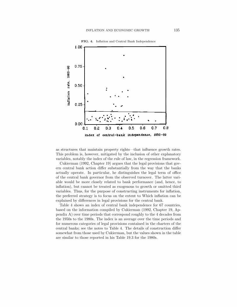
FIG. 4. Inflation and Central Bank Independence

iiqcx O, C6ITfLJ—p9IJJC IYq6b6uq6uc6 18Q0—86

OT OS 03 0( 02 0 0 08oooI I I

+ ++++++*++ +

+++++ + ++ +*.+ ++ ++ + + +4++

+ ++• 0S2 +

+- + + + +o +

++ +

020+

-4

C+

C

+

T00

CGUcLJ BUJ LTqcbGuqGucG

L!fTLG f 1Jpou 9.uq

as structures that maintain property rights—that influence growth rates.This problem is, however, mitigated by the inclusion of other explanatoryvariables, notably the index of the rule of law, in the regression framework.

Cukierman (1992, Chapter 19) argues that the legal provisions that gov-ern central bank action differ substantially from the way that the banksactually operate. In particular, he distinguishes the legal term of officeof the central bank governor from the observed turnover. The latter vari-able would be more closely related to bank performance (and, hence, toinflation), but cannot be treated as exogenous to growth or omitted thirdvariables. Thus, for the purpose of constructing instruments for inflation,the preferred strategy is to focus on the extent to Which inflation can beexplained by differences in legal provisions for the central bank.

Table 4 shows an index of central bank independence for 67 countries,based on the information compiled by Cukierman (1992, Chapter 19, Ap-pendix A) over time periods that correspond roughly to the 4 decades fromthe 1950s to the 1980s. The index is an average over the time periods andfor numerous categories of legal provisions contained in the charters of thecentral banks; see the notes to Table 4. The details of construction differsomewhat from those used by Cukierman, but the values shown in the tableare similar to those reported in his Table 19.3 for the 1980s.

136 ROBERT J. BARRO

TABLE 4.

Inflation Rates and Central Bank Independence

Country Index of Inflation Country Index of Inflation

bank rate, bank rate,

indep. 1960-90 indep. 1960-90

Vest Germany 0.71 0.037 South Africa 0.33 0.099

Switzerland 0.65 0.038 Nigeria 0.33 0.125

Austria 0.65 0.043 Malaysia 0.32 0.034

Egypt 0.57 0.094 Uganda 0.32 0.353

Denmark 0.53 0.069 Italy 0.31 0.088

Costa Rica 0.52 0.117 Finland 0.30 0.073

Greece 0.52 0.109 Sweden 0.30 0.067

United States 0.51 0.049 Singapore 0.30 0.034

Ethiopia 0.50 0.058 India 0.30 0.074

Ireland 0.50 0. 083 United Kingdom 0.30 0.077

Philippines 0.49 0.107 South Korea 0.29 0.113

Bahamas 0.48 0.063∗ China 0.29 0.039

Tanzania 0.48 0.133 Bolivia 0.29 0.466

Nicaragua 0.47 0.436 Uruguay 0.29 0.441

Israel 0.47 0.350 Brazil 0.28 0.723

Netherlands 0.47 0.045 Australia 0.27 0.067

Canada 0.47 0.054 Thailand 0.27 0.052

Venezuela 0.45 0.100 Western Samoa 0.26 0.112∗∗

Barbados 0.44 0.075 New Zealand 0.25 0.085

Argentina 0.44 0.891 Nepal 0.23 0.084

Honduras 0.44 0.058 Panama 0.23 0.033

Peru 0.44 0.606 Zimbabwe 0.22 0.074

Chile 0.43 0.416 Hungary 0.21 0.047

Turkey 0.42 0.235 Japan 0.20 0.054

Malta 0.42 0.035 Pakistan 0.19 0.072

Table 4 also contains the average inflation rate from 1960 to 1990 for the67 countries in my sample that have data on the index of central bank in-dependence. A comparison between the index and the inflation rate revealsa crucial problem; the correlation between the two variables is essentiallyzero, as in clear from Figure 4. This verdict is also maintained if one looksseparately over the three decades from the 1960s to the 1980s and if oneholds constant other possible determinants of inflation. In This broad sam-ple of countries, differences in legal provisions that ought to affect central

INFLATION AND ECONOMIC GROWTH 137

TABLE 4—Continued

Country Index of Inflation Country Index of Inflation

bank rate, bank rate,

indep. 1960-90 indep. 1960-90

Iceland 0.42 0.229 Colombia 0.19 0.170

Kenya 0.40 0.082 Spain 0.16 0.096

Luxembourg 0.40 0.044 Morocco 0.15 0.055

Zaire 0.39 0.357 Belgium 0.13 0.048

Mexico 0.37 0.227 Yugoslavia 0.12 0.395

Indonesia 0.36 0.366 Poland 0.12 0.293∗

Botswana 0.36 0.076 Norway 0.12 0.066

Ghana 0.35 0.256

France 0.34 0.064

Zambia 0.34 0.174∗ 1970-90∗∗ 1975-90Notes to Table 4: The index of central bank independence is computed fromdata in Cukierman (1992, Chapter 19, Appendix A). The index is a weightedaverage of the available data from 1950 to 1989 of legal provisions regarding1. appointment and dismissal of the governor (weight 1/6), 2. procedures forthe formulation of monetary pol icy (weight 1/6), 3. objectives of central bankpolicy (weight 1/6), and 4. limitations on lending by the central bank (weight1/2). The first category is an unweighted average of three underlying variablesthat involve the governors term of office and the procedures for appointmentand dismissal. The second category is an unweighted average of two variables,one indicating the location of the authority for setting monetary policy and theother specifying methods for resolving conflicts about policy. The third cate-gory relates to the prominence attached to price stability in the banks charter.The fourth category is an unweighted average of four variables: limitations onadvances, limitations on securitized lending, an indicator for the location of theauthority that prescribes lending terms, and the circle of potential borrowersfrom the central bank. For each underlying variable, Cukierman defines a scalefrom 0 to 1, where 0 indicates least favorable to central bank independence and1 indicates most favorable. The overall index shown in Table 4 runs correspond-ingly from 0 to 1. See Table 1 for a discuss ion of the inflation data.

bank independence have no explanatory power for inflation.7 This negativefinding is of considerable interest, because it suggests that low inflation can-not be attained merely by instituting legal changes that appear to promotea more independent central bank. However, the result also means thatwe have to search further for instruments to clarify the relation betweengrowth and inflation.8

7Cukierman’s (1992, Chapter 20) results concur with This finding, especially for sam-ples that beyond a small number of developed countries, the kind of sample used in mostof the on central bank independence.

8Cukierman, et al (1993) use as instruments the turnover rate of bank governors andthe average number of changes in bank leadership that occur within six months of a

138 ROBERT J. BARRO

2. Lagged InflationEarlier values of a country’s inflation rate have substantial explanatory

power for inflation.9 Lagged inflation would also be exogenous with respectto innovations in subsequent growth rates. Hence, if lagged inflation is usedas an instrument, then the estimated relation between growth and inflationwould not tend to reflect the short-run reverse effect of growth on inflation.

One problem, however, is that lagged inflation would reflect persistentcharacteristics of a country’s monetary institutions (such as the extent towhich policymakers have credibility), and these characteristics could becorrelated with omitted variables that are relevant to growth (such as theextent to which political institutions support the maintenance of propertyrights). The use of lagged inflation as an instrument would therefore notrule out the problems of interpretation that derive from omitted third vari-ables. However, the inclusion of the other explanatory variables in theregression framework lessens this problem. Another favorable element isthat the residuals from the growth equations are not significantly correlatedover the time periods.

Column 3 of Table 2 shows the estimated effect of inflation on the growthrate when lagged inflation (over the five years prior to each sample period) isused as an instrument. The estimated coefficient is −0.020 (0.007), similarto that found in column 1 when contemporaneous inflation is includedas an instrument. Thus, it seems that most of the estimated negativerelation between growth and inflation does not represent reverse short-term(negative) effects of growth on inflation.

The significant negative influence of inflation on growth still shows uponly when the high-inflation observations are included. The results are,however, again consistent with a linear relation and with stability over thetime periods. The standard deviation of inflation also remains insignifi-cant if it is added to the regressions (with lagged values of this standarddeviation included as instruments).

3. Prior Colonial StatusAnother possible instrument for inflation comes from the observation

that prior colonial status has substantial explanatory power for inflation.Table 5 breaks down averages of inflation rates from 1960 to 1990 by groups

change in government. These measures of actual bank independence have substantialexplanatory power for inflation but would not tend to be exogenous with respect togrowth.

9I have carried out SUR estimation of a panel system with the inflation rate as thedependent variable (for 1965-75, 1975-85, and 1985-90), where the independent vari-ables are lagged inflation and the other instrumental variables used in Table 2. Theestimated coefficient of lagged inflation is 0.74(0.06). The only other coefficients thatreach marginal significance are for log(GDP ), 0.037(0.019); the black-market premium,0.059 (0.033); the change in the terms of trade, −0.40 (0.22); and the rule-of-law index,−0.009 (0.005). The R2 values for the three periods are 0.55, 0.24, and 0.37.

INFLATION AND ECONOMIC GROWTH 139

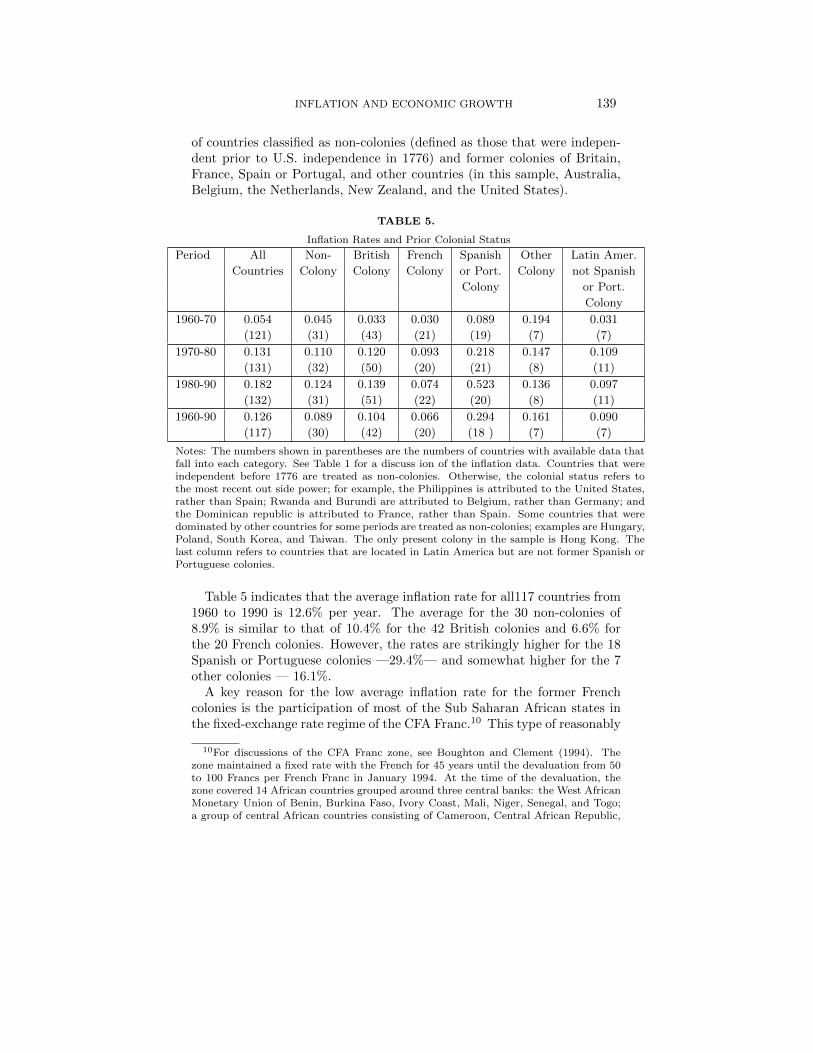
of countries classified as non-colonies (defined as those that were indepen-dent prior to U.S. independence in 1776) and former colonies of Britain,France, Spain or Portugal, and other countries (in this sample, Australia,Belgium, the Netherlands, New Zealand, and the United States).

TABLE 5.

Inflation Rates and Prior Colonial Status

Period All Non- British French Spanish Other Latin Amer.

Countries Colony Colony Colony or Port. Colony not Spanish

Colony or Port.

Colony

1960-70 0.054 0.045 0.033 0.030 0.089 0.194 0.031

(121) (31) (43) (21) (19) (7) (7)

1970-80 0.131 0.110 0.120 0.093 0.218 0.147 0.109

(131) (32) (50) (20) (21) (8) (11)

1980-90 0.182 0.124 0.139 0.074 0.523 0.136 0.097

(132) (31) (51) (22) (20) (8) (11)

1960-90 0.126 0.089 0.104 0.066 0.294 0.161 0.090

(117) (30) (42) (20) (18 ) (7) (7)

Notes: The numbers shown in parentheses are the numbers of countries with available data thatfall into each category. See Table 1 for a discuss ion of the inflation data. Countries that wereindependent before 1776 are treated as non-colonies. Otherwise, the colonial status refers tothe most recent out side power; for example, the Philippines is attributed to the United States,rather than Spain; Rwanda and Burundi are attributed to Belgium, rather than Germany; andthe Dominican republic is attributed to France, rather than Spain. Some countries that weredominated by other countries for some periods are treated as non-colonies; examples are Hungary,Poland, South Korea, and Taiwan. The only present colony in the sample is Hong Kong. Thelast column refers to countries that are located in Latin America but are not former Spanish orPortuguese colonies.

Table 5 indicates that the average inflation rate for all117 countries from1960 to 1990 is 12.6% per year. The average for the 30 non-colonies of8.9% is similar to that of 10.4% for the 42 British colonies and 6.6% forthe 20 French colonies. However, the rates are strikingly higher for the 18Spanish or Portuguese colonies —29.4%— and somewhat higher for the 7other colonies — 16.1%.

A key reason for the low average inflation rate for the former Frenchcolonies is the participation of most of the Sub Saharan African states inthe fixed-exchange rate regime of the CFA Franc.10 This type of reasonably

10For discussions of the CFA Franc zone, see Boughton and Clement (1994). Thezone maintained a fixed rate with the French for 45 years until the devaluation from 50to 100 Francs per French Franc in January 1994. At the time of the devaluation, thezone covered 14 African countries grouped around three central banks: the West AfricanMonetary Union of Benin, Burkina Faso, Ivory Coast, Mali, Niger, Senegal, and Togo;a group of central African countries consisting of Cameroon, Central African Republic,

140 ROBERT J. BARRO

exogenous commitment to relatively low inflation is exactly the kind ofexperiment that provides for a good instrument for inflation.

For many of the former British colonies, a significant element may betheir prior experience with British organized currency boards, anothersystem that tends to generate low inflation (see Schwartz [1993]). Theseboards involved, at one time or another before independence, most of theBritish colonies in Africa, the Caribbean, southeast Asia, and the mideast.

The high average inflation rate for the 16 former Spanish colonies inthe sample does not reflect, per se, their presence in Latin America. Forseven Latin American countries that are not former Spanish or Portuguesecolonies,11 the average inflation rate for 1960-90 is only 9.0%, virtually thesame as that for the non-colonies (see Table 5). Also, four former Por-tuguese colonies in Africa experienced the relatively high average inflationrate of around 20%.12 For Portugal and Spain themselves, the average in-flation rate of 10.9% for 1960-90 is well below the rate of 29.4% experiencedby their former colonies. However, 10.9% inflation is substantially higherthan that experienced by France (6.4%) and the United Kingdom (7.7%).

Column 4 of Table 2 shows the estimated effect of inflation on the growthrate of GDP when the instruments exclude contemporaneous or lagged in-flation but include indicators of prior colonial status. The two variablesused are a dummy for whether the country is a former Spanish or Por-tuguese colony and a dummy for whether the country is a former colony ofa country other than Britain, France, Spain, or Portugal.13 The estimated

Chad, Equatorial Guinea, and Gabon; and the Comoros. SomeC original members of thezone to establish independent currencies-Djibouti in 1949, Guinea in 1958, Mali in 1962(until it rejoined in 1984), Madagascar in 1963, Mauritania in 1973, and the Comoros in1981 (to set up its own form of CFA franc). Equatorial Guinea, Which joined in 1985,is the only member that is not a former colony of France (and not French-speaking).

11The seven in the sample are Barbados, Dominican Republic (attributed to Francerather than Spain; see the notes to Table 5), Guyana, Haiti, Jamaica, Suriname, andTrinidad & Tobago. Five other former British colonies in Latin America that are notin this sample — Bahamas, Belize, Grenada, St. Lucia and St. Vincent — experiencedthe relatively low average inflation rate of 6.9% from 1970 to 1990.

12These four are Angola, Cape Verde, Guinea-Bissau, and Mozambique. Data areunavailable for Cape Verde and Guinea-Bissau in the 1960s (prior to independence).The figures for Angola in the 1980s are rough estimates.

13I have carried out SUR estimation of a panel system with the inflation rate asthe dependent variable for(1965-75, 1975-85, and 1985-90), where the independent vari-ables are the two colony dummies and the other instrumental variables—mainly laggedvariables—used in Table 2. This system excludes lagged inflation (see n.6). The esti-mated coefficient on the Spain-Portugal colonial dummy is 0.14 (0.03) and that on thedummy for other colonies is 0.11(0.05). The R2 values are 0.38 for 1965-75, 0.14 for1975-85, and 0.10 for 1985-90. Thus, inflation is difficult to explain, especially if mostcontemporaneous variables and lagged inflation are excluded as regressors. Two variablesthat are sometimes suggested as determinants of inflation—trade openness (measuredby lagged ratios of exports and imports to GDP) and country size (measured by log ofpopulation)—are insignificant if added to the system. Years since independence also has

INFLATION AND ECONOMIC GROWTH 141

coefficient on the inflation rate is now −0.031 (0.008), somewhat higher inmagnitude than that found when contemporaneous or lagged inflation isused as an instrument. The significantly negative relation between growthand inflation again arises only when the high-inflation experiences are in-cluded in the sample. The results also continue to be stable over the timeperiods.

One question about the procedure is whether prior colonial status worksin the growth regressions only because it serves as an imperfect proxyfor Latin America, a region that is known to have experienced surpris-ingly weak economic growth (see, for example, the results in Barro [1991]).However, column 5 of Table 2 shows that if a dummy variable for LatinAmerica is included in the system (and the indicators of prior colonialstatus and the Latin America dummy are used as instruments), then theestimated coefficient of inflation remains negative and significant, −0.025(0.009). Moreover, the estimated coefficient on the Latin America dummyis only marginally significant, −0.0060 (0.0034). The results are basicallythe same if the Latin America dummy is added to the system from column1 of Table 2, in which contemporaneous inflation is used as an instrument.It therefore appears that much of the estimated effect of a Latin Americadummy on growth rates in previous research reflected a proxying of thisdummy for high inflation. In particular, the negative effect of inflation ongrowth does not just reflect the tendency for many high-inflation countriesto be in Latin America.

5. ESTIMATED EFFECTS OF INFLATION ONINVESTMENT

A likely channel by Which inflation decreases growth is through a re-duction in the propensity to invest (This effect is already held constantby the presence of the investment ratio in the growth regressions.) I haveinvestigated the determination of the ratio of investment to GDP withina framework that parallels the one set out in Table 2. The results are inTable 6.

In the case of the investment ratio, the use of instruments turns out tobe crucial for isolating a negative effect of inflation. In Column 1 of Table6, which uses contemporaneous inflation as an instrument, the estimatedcoefficient on the inflation rate is virtually zero, −0.001 (0.011). In con-trast, the result in column 2 with lagged inflation used as an instrumentis −0.059 (0.017). Similarly, the result in column 3 with the indicatorsof prior colonial status used as instruments is −0.044 (0.022). The lasttwo estimates imply that an increase in average inflation by ten percent-

no explanatory power for inflation. This result may arise because the former colonies ofSpain and Portugal in Latin America became independent at roughly the same time.

142 ROBERT J. BARRO

age points per year would lower the investment ratio on impact by 0.4-0.6percentage points.

TABLE 6.

Regressions for Investment Ratio

Variable (1) (2) (3)

log(GDP) −0.008 −0.011 −0.011

(0.010) (0.011) (0.010)

male 0.016 0.010 0.013

schooling (0.011) (0.012) (0.011)

female −0.018 −0.012 −0.016

schooling (0.012) (0.013) (0.013)

log(life 0.228 0.242 0.231

expectancy) (0.045) (0.047) (0.046)

log(fertility −0.010 −0.010 −0.013

rate) (0.018) (0.019) (0.019)

govt. consump −0.172 −0.215 −0.220

ratio (0.083) (0.088) (0.087)

public educ. 0.18 −0.06 0.09

spending ratio (0.27) (0.29) (0.28)

black-market −0.017 0.001 0.000

premium (0.013) (0.014) (0.015)

rule-of-law 0.0150 0.0151 0.0146

index (0.0034) (0.0036) (0.0035)

terms-of-trade 0.047 0.060 0.059

change (0.062) (0.070) (0.067)

democracy 0.092 0.111 0.103

index (0.059) (0.059) (0.022)

R2 0.64, 0.62, 0.67 0.64, 0.61, 0.62 0.65, 0.62, 0.66

number of 78, 89, 78, 89, 78,89,

observations 84 84 84

Notes: The systems have three equations, where the dependent variables arethe ratios of real gross investment to real GDP for 1965-75, 1975-85, and1985-90. See the notes to Table 2 for definitions of the variables. Estimationis by instrumental variables. Column 1 includes inflation as an instrument.Column 2 uses inflation over the previous 5 years as an instrument. Column 3uses prior colonial status as instruments. See the notes to Table 2 for descriptions of the other instruments.

Even when the instruments are used, the adverse effect of inflation oninvestment shows up clearly only when the high—inflation observations areincluded in the sample. This finding accords with the results for growthrates.

INFLATION AND ECONOMIC GROWTH 143

6. CONCLUDING OBSERVATIONS

A major finding from the empirical analysis is that the estimated effectsof inflation on growth and investment are significantly negative when someplausible instruments are used in the statistical procedures. Thus, thereis some reason to believe that the relations reflect causation from higherlong-term inflation to reduced growth and investment.

It should be stressed that the clear evidence for adverse effects of inflationcomes from the experiences of high inflation. The magnitudes of effects arealso not that large; for example, an increase in the average inflation rateby10 percentage points per year is estimated to lower the growth rate ofreal per capita GDP (on impact) by 0.2-0.3 percentage points per year.

Some people have reacted to these kinds of findings by expressing skep-ticism about the value of cross-country empirical work. In fact, the widedifferences in inflation experiences offered by the cross section provide thebest opportunity for ascertaining the long-term effects of inflation and othervariables on economic performance. If the effects cannot be detected ac-curately in this kind of sample, then they probably cannot be pinpointedanywhere else. In particular, the usual focus on annual or quarterly timeseries of 30-40 years for one or a few countries is much less promising.

In any event, the apparently small estimated effects of inflation on growthare misleading. Over long periods, these changes in growth rates havedramatic effects on standards of living. For example, a reduction in thegrowth rate by 0.2-0.3 percentage points per year (produced on impactby10 percentage points more of average inflation) means that the level ofreal gross domestic product would be lowered after 30 years by 4-7%.14 Inmid 1995, the U.S. gross domestic product was over $7 trillion; 4-7% of Thisamount is 1300-500 billion, more than enough to justify a keen interest inprice stability.

REFERENCES

Alesina, Alberto and Lawrence H. Summers, 1993. Central Bank Independenceand Macroeconomic Performance: Some Comparative Evidence. Journal of Money,

14In the model, the fall in the growth rate by 0.2-0.3 percent per year applies onimpact in response to a permanent increase in the inflation rate. The growth rate wouldalso decrease for a long time thereafter, but the of This decrease diminishes toward zeroas the economy converges back to its (unchanged) long-run growth rate. Hence, in thevery long run, the effect of higher inflation is a path with a permanently lower level ofoutput, not a reduced growth rate. The numerical estimates for the reduced level ofoutput after 30 years take account of these dynamic effects. The calculation depends onthe economy’s rate of convergence to its long-term growth rate (assumed, based on theempirical estimates, to be 2-3 percent per year). Also, the computations unrealisticallyneglect any responses of the other explanatory variables, such as the human-capitalmeasures and the fertility rate.

144 ROBERT J. BARRO

Credit, and Banking 25, 151-162.

Bade, Robin and J. Michael Parkin, 1982. Central Bank Laws and Monetary Policy.Unpublished, University of Western Ontario.

Barro, Robert J., 1991. Economic Growth in a Cross Section of Countries. QuarterlyJournal of Economics 106, 407-433.

Barro, Robert J., 1996. Democracy and Growth. Journal of Economic Growth 1,forthcoming.

Barro, Robert J. and Xavier Sala-i-Martin, 1995. Economic Growth. New York, Mc-Graw Hill.

Bollen, Kenneth A., 1990. Political Democracy: Conceptual and Measurement Traps.Studies in Comparative International Development Spring, 7-24.

Boughton, James M., 1991. The CFA Franc Zone: Currency Union and MonetaryStandard. International Monetary Fund working paper 91/133 (forthcoming in An-thony Courakis and George Tavlas, eds., Monetary Integration, Cambridge, Cam-bridge University Press).

Briault, Clive, 1995. The Costs of Inflation. Bank of England Quarterly Bulletin 35,33-45.

Clement, Jean A. P., 1994. Striving for Stability: CFA Franc Realignment. Finance& Development June, 10-13.

Cukierman, Alex, 1992. Central Bank Strategy, Credibility, and Independence. MITPress, Cambridge MA.

Cukierman, Alex, Pantelis Kalaitzidakis, Lawrence H. Summers, and Steven B. Webb,1993. Central Bank Independence, Growth, Investment, and Real Rates. Carnegi-Rochester Conference Series on Public Policy 39, 95-140.

Fischer, Stanley, 1993. The Role of Macroeconomic Factors in Growth. Journal ofMonetary Economics 32, 485-512.

Gastil, Raymond D. and followers, 1982. Freedom in the World. Westport CT, Green-wood Press.

Grier, Kevin B. and Gordon Tullock, 1989. An Empirical Analysis of Cross-NationalEconomic Growth. Journal of Monetary Economics 24, 259-276.

Grilli, Vittorio, Donato Masciandaro, and Guido Tabellini, 1991. Political and Mon-etary Institutions and Public Finance Policies in the Industrial Countries. EconomicPolicy 13, 341-392.

Knack, Stephen and Philip Keefer, 1994. Institutions and Economic Performance:Cross-Country Tests Using Alternative Institutional Measures. Unpublished paper,American University, February.

Kormendi, Roger C. and Philip G. Meguire, 1985. Macroeconomic Determinants ofGrowth: Cross-Country Evidence. Journal of Monetary Economics 16, 141-163.

Logue, Dennis E. and Thomas D. Willett, 1976. A Note on the Relationship betweenthe Rate and Variability of Inflation. Economica 43, 151-158.

Mankiw, N. Gregory, David Romer, and David N. Weil, 1992. A Contribution to theEmpirics of Economic Growth. Quarterly Journal of Economics 107, 2.

Okun, Arthur M., 1971. The Mirage of Steady Inflation. Brookings Papers on Eco-nomic Activity 2, 485-498.

Schwartz, Anna J., 1993. Currency Boards: Their Past, Present, and Possible FutureRole. Carnegi-Rochester Conference Series on Public Policy 39, 147-187.

Summers, Robert and Alan Heston, 1993. Penn World Tables, Version 5.5. Availablefrom the National Bureau of Economic Research, Cambridge MA.