Impulse

This topic is designed to give you the big picture of AFT Impulse's layout and structure. Some of the more basic concepts will be used to build an eight-pipe, eight-junction model to solve a waterhammer problem published in the literature (Karney, et al., 1992). This system has reservoirs, a surge tank, a relief valve and an exit valve.

A number of other example model discussions are included in a Help file distributed with AFT Impulse called ImpulseExamples.hlp. It can be opened from the Help menu by choosing "Show Examples".

Step 1. Start AFT Impulse

Ø To start AFT Impulse, click Start on the Windows taskbar, choose Programs, then AFT Products then AFT Impulse. (This refers to the standard menu items created by setup. You may have chosen to specify a different menu item).

When you start AFT Impulse, the Workspace window is always the active (large) window. The Workspace window is one of five Primary Windows.

After AFT Impulse loads, you will notice four windows in the lower part of the AFT Impulse window; these represent four of the five Primary Windows that are currently minimized (see Figure 2.1). The AFT Impulse window acts as a container for the five Primary Windows.

Figure 2.1 The Workspace window is where the model is built

The Workspace window

The Workspace window is the primary vehicle for building your model. This window has two main areas: the Toolbox and the Workspace itself. The Toolbox is the bundle of tools on the far left. The Workspace takes up the rest of the window.

You will build your waterhammer model on the Workspace using the Toolbox tools. At the top of the Toolbox are four drawing tools below the Shortcut button. The Selection Drawing tool, on the upper left, is useful for selecting groups of objects on the Workspace for editing or moving. The Pipe Drawing tool, on the upper right, is used to draw new pipes on the Workspace. Below these two tools are the Zoom Select tool and the Annotation tool. The Zoom Select tool allows you to draw a box on the Workspace after which AFT Impulse will zoom into that area. The Annotation tool allows you to create annotations and auxiliary graphics.

Below the four drawing tools are nineteen icons that represent the different types of junctions available in AFT Impulse. Junctions are components that connect pipes and also influence the pressure or flow behavior of the pipe system. The nineteen junction icons can be dragged from the Toolbox and dropped onto the Workspace.

When you pass your mouse pointer over any of the Toolbox tools, a Tool Tip identifies the tool's function.

Step 2. Lay out the model

To lay out the walk-through model, you will place the two reservoir junctions, three branch junctions, a surge tank junction, a relief valve junction, and a valve junction on the Workspace. Then you will connect the junctions with pipes.

A. Place the first reservoir

Ø To start, drag a reservoir junction from the Toolbox and drop it on the Workspace. Figure 2.2a shows the Workspace with one reservoir.

Walk Through Example

of 24Walk Through Example

20/09/2011mk:@MSITStore:C:\AFT%20Products\Impulse%204.0%20Demo\IMPULSE.CHM::/...

Figure 2.2a Walk Through Model with one reservoir placed

Objects and ID numbers

Items placed on the Workspace are called objects. All objects are derived directly or indirectly from the Toolbox. AFT Impulse uses three types of objects: pipes, junctions and annotations.

All pipe and junction objects on the Workspace have an associated ID number. For junctions, this number is, by default, placed directly above the junction and prefixed with the letter “J”. Pipe ID numbers are prefixed with the letter “P”. You can optionally choose to display either or both the ID number and the name of a pipe or junction. You also can drag the ID number/name text to a different location to improve visibility.

The Reservoir you have created on the Workspace will take on the default ID number of 1. You can change this to any desired number greater than zero and up to 30,000.

Editing on the Workspace

Once on the Workspace, junction objects can be moved to new locations and edited with the features on the Edit menu. Cutting, copying, and pasting are all supported. A single level of undo is available for all editing operations.

Note: The relative location of objects in AFT Impulse is not important. Distances and heights are defined through dialog boxes. The relative locations on the Workspace establish the connectivity of the objects, but have no bearing on the actual length or elevation relationships.

B. Place the first branch

Ø Next, drag a branch junction from the Toolbox and drop it to the lower right of the reservoir J1. This becomes junction J2 (Figure 2.2b).



Figure 2.2b Walk Through Model with one reservoir and one branch placed

C. Place surge tank

Ø Now, drag a surge tank junction from the Toolbox and drop it to the right of the reservoir J1. This junction takes on the number J3 (Figure 2.2c).

Figure 2.2c Walk Through Model after placing the Surge Tank

D. Place the second reservoir

The second reservoir can be created the same way as the first one or it can be derived from the existing reservoir.

Ø To create a second reservoir from the existing one, select junction J1 by clicking it with the mouse. A red outline will surround the junction. Open the Edit menu and choose Duplicate. If you like, you can Undo the Duplicate operation and then Redo it to see how these editing features work.

Drag the new reservoir junction icon to the upper right of the Workspace. This is junction J4 (Figure 2.2d).

Figure 2.2d Walk Through Model after placing the second Reservoir

E. Add the remaining junctions

Next add the four remaining junctions - two branches, a regular valve and a relief valve (Figure 2.2e).



Figure 2.2e Walk Through Model after placing all junctions

Ø To add a branch junction, select a Branch from the Toolbox and place it on the Workspace as shown in Figure 2.2e. The Branch will take on the default number J5. Similarly, add another branch at junction J6.

Ø Add valve junctions by selecting the junction icons from the Toolbox and placing them on the Workspace as shown in Figure 2.2e. These junctions will become J7 and J8, respectively.

Ø Before continuing, save the work you have done so far. Choose Save As from the File menu and enter a file name ("WalkThru", perhaps) and AFT Impulse will append the “.IMP” extension to the file name.

F. Draw a pipe between J1 and J2

Now that you have the eight junctions, you need to connect them with pipes.

Ø To create a pipe, click on the Pipe Drawing tool icon. The pointer will change to a cross-hair when you move it over the Workspace. Draw a pipe below the junctions, similar to that shown in Figure 2.2f.

The pipe object on the Workspace has an ID number (P1) shown near the center of the pipe.

Figure 2.2f Walk Through Model after drawing first pipe

Ø To place the pipe between J1 and J2, grab the pipe in the center with the mouse and drag it so that its left endpoint falls within the J1 Reservoir icon and drop it there. Next, grab the right endpoint of the pipe and stretch the pipe, dragging it until the endpoint terminates within the J2 Branch icon (see Figure 2.2g).



Figure 2.2g Walk Through Model after placing first pipe

Reference positive flow direction

Located on the pipe is an arrow that indicates the reference positive flow direction for the pipe. AFT Impulse assigns a flow direction corresponding to the direction in which the pipe is drawn. You can reverse the reference positive flow direction by choosing Reverse Direction from the Arrange menu or selecting the reverse direction button on the Toolbar.

The reference positive flow direction indicates which direction is considered positive. If the reference positive direction is the opposite of that obtained by the Solver, the output will show the flow rate as a negative number.

G. Add the remaining pipes

A quicker way to add a pipe is to draw it directly between the desired junctions.

Ø Activate the pipe drawing tool again and press the mouse button down on the J2 Branch. Stretch the pipe up to the J3 Surge Tank and release the mouse button. Draw a third pipe from the J3 Surge Tank to the J4 Reservoir. Draw a fourth pipe from the J3 Surge Tank to the J5 Branch. Draw a fifth pipe from the J6 Branch to the J5 Branch. Draw a sixth pipe from the J2 Branch to the J6 Branch. Draw a seventh pipe from the J6 Branch to the J7 Valve.. Finally, draw an eight pipe from the J6 Branch to the J8 Valve. Your model should now look similar to Figure 2.2h.

At this point all the objects in the model are graphically connected. Save the model by selecting Save in the File menu or by clicking on the diskette button on the Toolbar.

Figure 2.2h Walk Through Model with all pipes and junctions placed

Note: It is generally desirable to lock your objects to the Workspace once they have been placed. This prevents accidental movement



and disruption of the connections. You can lock all the objects by choosing Select All from the Edit menu, then selecting Lock Object from the Arrange menu. The lock button on the Toolbar will appear depressed indicating it is in an enabled state, and will remain so as long as any selected object is locked. Alternatively, you can use the grid feature enabled on the Workspace Preferences window and specify that the pipes and junctions snap to grid.

Step 3. Set the unit preferences

Ø Open the Parameter and Units Preferences window from the Options menu. This Walk Through model is in metric units. The default in AFT Impulse is to offer both metric and traditional English units to the user, with English as the default. For consistency, we want to use metric as the default for this model, and we can specify that here.

Ø Select the Unit Preferences tab and then select the Default Unit System as SI. Click the Apply Default Units button. See Figure 2.3. Finally click OK to close the window.

Figure 2.3 The Parameter and Unit Preferences window allows you to specify the default unit system

Step 4. Complete the first three checklist requirements

Ø Next, click the checkmark on the Toolbar that runs across the top of the AFT Impulse window. This opens the Checklist window (see Figure 2.4). The checklist contains six items. Each item needs to be completed before AFT Impulse allows you to run the Solver.

The Status Bar at the bottom of the AFT Impulse window also reflects the state of each checklist item (see Figure 2.1). Once the checklist is complete, the Model Status light in the lower left corner turns from red to green.

Figure 2.4 The Checklist tracks the model’s status

A. Specify Steady Solution Control

The first item, Specify Steady Solution Control, is always checked when you start AFT Impulse because AFT Impulse assigns default solution control parameters for the steady-state part of the analysis. In general, you do not need to adjust Steady Solution Control values. If necessary, you can make adjustments by opening the Steady Solution Control window from the Analysis menu.

B. Specify output control

The second item on the checklist is Specify Output Control. Like Solution Control, this item is always checked when you start AFT Impulse. Default Output Control parameters and a default title are assigned.

You may want to add a descriptive title for the model. To do this, open the Output Control window (see Figure 2.5) and enter a title on



the General tab. In addition, this window allows you to select the specific output parameters you want in your output. You also can choose the units for the output.

Ø Close the checklist and select Output Control from the Analysis menu. (Figure 2.5 shows the Output Control window). Click the General Output tab, enter a new title (if you like you can title this “Transient With Surge Tank”), then click OK to accept the title and other default data.

Figure 2.5 The Output Control window lets you customize the output

C. Specify system properties

The third item on the checklist is Specify System Properties. To complete this item, you must open the System Properties window (see Figure 2.6). This window allows you to specify your fluid properties (density, dynamic viscosity, bulk modulus and optional vapor pressure), viscosity model, gravitational acceleration and atmospheric pressure.



Figure 2.6 The System Properties window lets you enter physical properties of the fluid

For models with variable fluid properties, the values for density, viscosity and bulk modulus are default fluid properties. You can then enter different property values, if desired, for any pipe in the Pipe Specifications window.

You can model the fluid properties in one of five ways.

1. Unspecified fluid -- This fluid model allows you to directly type in the density, viscosity, bulk modulus and vapor pressure.

2. AFT Standard fluid -- This fluid model accesses fluid data from the AFT Standard database. These fluid properties are either temperature dependent or dependent on the solids concentration. You type in the desired condition (e.g., temperature), click the Calculate Properties button and the required properties are calculated. Users can add their own fluids to this database. Custom fluids are created by opening the Fluid Database window from the AFT Impulse Database menu or by clicking the Edit Fluid List button in the System Properties window.

3. Chempak Fluid -- This fluid model allows you to select a single fluid from the Chempak database list. These fluid properties are pressure and temperature dependent, although some are temperature dependent only. Chempak is an optional add-on to AFT Impulse.

4. Chempak Mixture -- This fluid model allows you to create a liquid mixture from among the Chempak database fluids. These fluid properties are pressure and temperature dependent. Upon entering a pressure, AFT Impulse will display a temperature range applicable to the liquid. Chempak is an optional add-on to AFT Impulse.

5. Water Data from ASME Steam Tables -- As its name implies, this fluid model obtains water properties from ASME steam tables. This model is pressure and temperature dependent.

Ø Select System Properties from the Analysis menu to open the System Properties window. For this example, select the AFT Standard fluid option, then choose “Water at 1 atm” from the list and click the Add to Model button. The properties for AFT Standard water are given only as a function of temperature. Enter 20? C in the temperature box, click the Calculate Properties button and click OK.

Ø Open the checklist once more or observe the Status Bar and you should now see the third item checked off.

Step 5. Define the model components (checklist item #4)

The fourth item on the checklist, Define All Pipes and Junctions, is not as straightforward to satisfy as the first three. This item encompasses the proper input data and connectivity for all pipes and junctions.

Object status

Every pipe and junction has an object status. The object status tells you whether the object is defined according to AFT Impulse's requirements. To see the status of the objects in your model, click the floodlight on the Toolbar (alternatively, you could choose Show Object Status from the View menu). Each time you click the floodlight, Show Object Status is toggled on or off.

When Show Object Status is on, the ID numbers for all undefined pipes and junctions are displayed in red on the Workspace. Objects that are completely defined have their ID numbers displayed in black. (These colors are configurable through Workspace Preferences from the Options menu.)

Because you have not yet defined the pipes and junctions in this sample problem, all the objects' ID numbers will change to red when you turn on Show Object Status.



A. Define Reservoir J1

Ø To define the first reservoir, open the J1 Reservoir Specifications window by double-clicking on the J1 icon. Enter in a reservoir surface elevation of 200 meters. You can assign any unit of length found in the adjacent drop-down list box of units.

Note: You can also open an object's Specifications window by selecting the object (clicking on it) and then either pressing the Enter key or by clicking the Open Pipe/Jct Window icon on the Toolbar.

Ø Enter surface pressure of 1 atmosphere (atm) and a reservoir depth of 50 meters in the table on the Pipe Depth and Loss Coefficient tab.

Note: You can specify preferred units for many parameters (such as meters for length) in the Parameter and Unit Preferences window.

You can give the component a name, if desired, by entering it in the Name field at the top of the window. In Figure 2.7, the name of this reservoir is Supply Tank A. By default the junction’s name is the junction type. The name can be displayed on the Workspace, Visual Report or in the Output.

Figure 2.7 The Reservoir Specifications window for J1

Most junction types can be entered into a custom database allowing the junction to be used multiple times or shared between users. To select a junction from the custom database, choose the desired junction from the Database list. The current junction will get the properties from the database component.

The Same As Jct… list will show all the junctions of the same type in the model. This will copy selected parameters from an existing junction in the model to the current junction.

The pipe table on the Pipe Depth and Loss Coefficients tab allows you to specify entrance and exit loss factors for each pipe connected to the reservoir (in this case there is one). You can enter standard losses by selecting the option buttons at the right. The default selection is the Custom option with loss factors specified as zero. To later change the loss factors, click within the pipe table and enter the loss. You can also specify a depth for the pipe.

The Optional tab allows you to enter different types of optional data. You can select whether the junction number, name, or both are displayed on the Workspace. Some junction types also allow you to specify an initial pressure as well as other junction specific data. The junction icon graphic can be changed, as can the size of the icon. Design factors can be entered for most junctions, which are applied to the pressure loss calculations for the junction in order to give additional safety margin to the model.

Each junction has a tab for notes, allowing you to enter text describing the junction or documenting any assumptions.

The highlight feature displays all the required information in the Specifications window in light blue. The highlight is on by default. You can toggle the highlight off and on by double-clicking anywhere in the window or by pressing the F2 key. The highlight feature can also be turned on or off by selecting it on the Options menu.

Ø Click OK. If Show Object Status is turned on, you should see the J1 ID number turn black again, telling you that J1 is now completely defined.

The Inspection feature

You can check the input parameters for J1 quickly, in read-only fashion, by using the Inspection feature. Position the mouse pointer on J1 and hold down the right mouse button. An information box appears, as shown in Figure 2.8.

Inspecting is a faster way of examining the input in an object than opening the Specifications window.



Figure 2.8 Inspecting from the Workspace with right mouse button

B. Define Branch J2

Ø Open the J2 Branch Specifications window . In this window, three connecting pipes will be displayed in the pipe table area. Branches are connector points for up to twenty-five pipes.

Ø Enter an elevation of 100 meters for the J2 Branch junction (an elevation must be defined for all junctions). You can also specify a transient flow source or sink at the junction.

Ø Click the Optional tab and enter an imposed flow rate of -2 m3/sec (the negative sign means that the flow is out of the junction – a flow sink).

Ø Click OK to accept the input and exit the window.

C. Define Surge Tank J3

Ø Open the J3 Surge Tank Specifications window and enter an elevation of 150 meters. Enter a tank area of (a constant) 5 square meters. This is the cross-sectional area of the surge tank, which allows AFT Impulse to determine how the surface elevation changes with a given amount of flow into the tank. Leave the tank height blank. This is the physical height of the tank. If a height is entered, AFT Impulse will not allow the liquid height to exceed the tank height (which results in spillage over the tank edge). Figure 2.9 shows the Surge Tank window.

Figure 2.9 The Surge Tank specifications window for J3



Ø Click the check box to Model Short Connector Pipe. This allows you to model a short pipe which is lumped together with the surge tank for each solution. The data for the connector pipe is as follows: Friction factor is 0.02, Pipe Diameter is 0.5 meters, Pipe Area is 0.1963 square meters (it is cylindrical), Pipe Length is 30 meters, and Elevation Change is 30 meters (i.e., the pipe is vertical because the elevation change is the same as the length).

You also can model a flow restrictor (e.g., orifice) if one exists.

D. Define Reservoir J4 and Branches J5 and J6

Ø Open the J4 Reservoir Specifications window. Enter a surface elevation of 175 meters and a depth of 25 meters (on the Pipe Depth… tab). Leave surface pressure as atmospheric.

Ø Open the J5 Branch Specifications window. Enter an elevation of 100 meters and an imposed flow of -1 m3/sec (on the Optional tab). This is an outflow type of branch similar to J2.

Ø Open the J6 Branch Specifications window. Enter an elevation of 50 meters. There is no imposed flow at this junction.

E. Define Valve J7

Ø Open the J7 Valve Specifications window. Valve junctions connect with two pipes if they are internal and one pipe if they are exit valves. This will be an exit valve. Enter an elevation of 25 meters and select the Exit Valve option at the lower left. Choose Head and enter an exit pressure of 25 meters, which is equivalent to 1 atm (because exit atmospheric head is equal to elevation).

Ø Choose the loss model as Cv. This valve will initiate the transient for this system. Until the valve changes position, the entire pipe system is in a steady-state condition. Enter a Cv of 2392.6. This is the steady-state value.

Ø Select the Transient Data tab. In this transient the valve partially closes over a period of 10 seconds, then holds steady at the new position for the remainder of the simulation. Enter the following Cv vs. time data in the table (see Figure 2.10):

Figure 2.10 Valve Specifications for J7 initiates the transient for the system

F. Define Valve J8

Ø Open the J8 Valve Specifications window. For this example, a regular valve junction will be used to model the behavior of a relief valve. This relief valve will vent to an external source, so it should be modeled as an Exit Valve, with an exit pressure of 1 atm. Enter an elevation of 50 meters.

Ø Choose the loss model as Cv and enter a Cv value of 651.2. This represents the valve's Cv after it fully opens. The valve remains closed until the cracking pressure is exceeded (defined on the Transient Data tab), at which point the valve opens to relieve pressure.

Ø Click the Transient Data tab and select the Single Event option for the Initiation of Transient. Select Pressure Stagnation at Pipe as the Event Type, Greater Than or Equal To as the Condition, and a Value of 1.688 MPa at the outlet of Pipe 8. This Event represents the cracking pressure required initiate the opening transient of the relief valve.

Time Cv 0 2392.6

10 797.4 100 797.4



Enter the valve transient Cv data below in the Transient Data table. (See Figure 10a):

The data represents the valve initially closed at time zero. Time zero is the moment of cracking. The valve then opens and gradually closes again over a period of 60 seconds.

Because the valve is closed initially, set the valve Special Condition on the Optional Data tab to Closed.

Figure 2.10a Valve Specifications for J8 initiates the transient for the relief valve

G. Define Pipe P1

The next step is to specify all the pipes. To open the Pipe Specifications window, double-click the pipe object on the Workspace.

Ø First open the Pipe Specifications window for Pipe P1 (Figure 2.11). Choose the Pipe Material as Unspecified, choose the User Specified Wavespeed option, and select the Friction Model Data Set as Unspecified with the Friction Model as "Explicit Friction Factor". Enter a length of 1001.2 meters, a diameter of 1.5 meters, and a friction factor of 0.012.

Note: This example from Karney assumes all friction factors are known ahead of time. Normally this will not be the case. In most cases you will access the roughness for the pipe from the pipe material database supplied with AFT Impulse, or input your own roughness value. Then AFT Impulse will calculate the friction factor using standard methods (see Roughness Models).

The wavespeed is a very important parameter in waterhammer analysis. The wavespeed can be calculated with reasonable accuracy from fluid and pipe data, or it may be available from test data or industry publications. In this example the wavespeed is known to be 996.3 meters per second. Therefore, the wavespeed can be entered directly. This is why we selected the User Specified Wavespeed option. If the wavespeed were not known (which is typical), then the Calculated Wavespeed option would be preferred. In this case, data would be required for pipe wall thickness, modulus of elasticity, Poisson Ratio, and pipe support details. Data for pipe wall thickness, modulus of elasticity, Poisson Ratio are built into the pipe material databases supplied with AFT Impulse.

The Pipe Specifications window

The Pipe Specifications window offers control over all important flow system parameters related to pipes.

The Inspect feature also works within the Pipe Specifications window. To Inspect a connected junction, position the mouse pointer on the connected junction's ID number and hold down the right mouse button. This is helpful when you want to quickly check the properties of connecting objects. (You can also use this feature in junction Specifications windows for checking connected pipe properties.)

By double-clicking the connected junction number, you can jump directly to the junction's Specifications window. Or you can click the Jump button to jump to any other part of your model.

Time Cv 0 0 3 651.2

63 0 100 0



Figure 2.11 Pipe Specifications window for P1

H. Define Pipes P2 through P7

Ø Open the Specifications window for each of the other pipes and enter the following data (pipe 1 data was just entered so ignore it):

After entering the data for all the pipes, the fourth checklist item should be completed. If it is not, see if the Show Object Status is on. If not, select Show Object Status from the View menu or toolbar. If the fourth checklist item is not completed at this point, see if any of the pipes or junctions have their number displayed in red. If so, you did not enter all the data for that item.

Ø Before continuing the model, save it to file one more time. It is also a good idea to review the input using the Model Data window.

Reviewing input in Model Data window

The Model Data window is shown in Figure 2.12. To change to this window, you can select it from the Window menu, the Toolbar, pressing Ctrl-M, clicking anywhere in the Model Data window if it has been restored or, if minimized, clicking on the minimized window at the bottom of the screen and restoring it. The Model Data window gives you a text-based perspective of your model. Selections can be copied to the clipboard and transferred into other Windows programs, or printed out for review. Figure 2.13 shows an expanded view of the Transient Data tab from Figure 2.12. Here all transient input data for the model is shown.

The Model Data window allows access to all Specifications windows by double-clicking the appropriate ID number in the far left column of the table. You may want to try this right now.

Pipe Length Diameter Friction Wavespeed

(meters) (meters) Factor (meters/sec)

1 1001.2 1.5 0.012 996.3

2 2000 1 0.013 995.3

3 2000 0.75 0.014 995

4 502.5 0.5 0.015 1000

5 502.5 0.5 0.015 1000

6 1001.2 1 0.014 996.3

7 2000.2 0.75 0.013 995.1

8 100.12 1 0.014 996.3



Figure 2.12 The Model Data window shows the input data in text form

Figure 2.13 The Transient Data tab in the Model Data Junction data area shows all transient data entered

Step 6. Complete the last two checklist requirements

A. Specify pipe sectioning

The fifth checklist item is Section Pipes. This window cannot be opened until sufficient data is entered previously. First, the fluid must be selected (we did this Step 4C when we entered System Properties). And second, all pipes must have a length and wavespeed entered. After this data has been entered, the pipes can be sectioned. The Section Pipes window helps divide the pipes into computation sections in a manner which is consistent with the Method of Characteristics (MOC).

Ø Select Section Pipes on the Analysis menu to display the Section Pipes Window (Figure 2.14). For this model the controlling pipe is P8. This is the pipe with the shortest end-to-end communication time (i.e., L/a – the length divided by the wavespeed). To satisfy the MOC, the following equation must be applied:

where n is the number of sections in pipe i, L is the length, and a is the wavespeed. The ?t is the time step. Since all pipes in the network must be solved together, the same time step must be used for each pipe. With a given length and wavespeed for each pipe, it can be seen from the above equation that it is unlikely that the number of required sections, n, for each pipe will be a whole number.

To address this situation, it is helpful to recognize that the wavespeed, a, is the least certain input parameter. It is therefore acceptable to allow up to a 15% uncertainty in wavespeed. By adjusting the wavespeed for each pipe within this tolerance the sectioning can be made to come out as whole numbers for each pipe. The Section Pipes window automates this process by searching for sectioning which satisfies the required tolerance.

You can specify the tolerance on wavespeed by entering it into the Max. Percentage Error. The minimum and maximum allowable sections in the controlling pipe narrows the search space. Also, the Percentage Increment directs the routine in how fine to search the search space.

This model has been specified by Karney in such a way that the pipe sectioning falls closely along whole numbers.



Figure 2.14 The Section Pipes window automates the sectioning process and calculates the time step.

Ø For Min. and Max. Sections in Controlling Pipe enter 1 section for each. Limit the Max Error to 1% for the search (usually 5 or 10% is fine). Check the box for Sort Sectioning by Minimum Error. Then click the Search button.

A list of possible sectioning is displayed. Click the top line with 1.0000 sections in the controlling pipe. The resulting time step will be displayed as 0.100492 seconds.

The sectioning and resulting errors in the remaining pipes are displayed in the table near the bottom. Click OK and the fifth checklist item should be completed.

Note: The error in the Section Pipes window relates only to sectioning roundoff and not to overall model accuracy.

B. Specify transient control

The sixth and final checklist item is Transient Control. This window allows you to specify the time at which the transient starts and ends, as well as how much data to include in the output file.



Figure 2.15 The Transient Control window offers features to specify the time span for the transient and what output data is written

Ø Select Transient Control on the Analysis menu to display the Transient Control window (Figure 2.15). Enter zero for Start Time and 65 for Stop Time.

The Transient Control window lets you enable or disable transient cavitation modeling. It also offers control over how AFT Impulse should respond to artificial transients. Artificial transients are a problem that can sometimes occur when steady-state and transient conditions are inconsistent.

Data can be saved for all pipe stations or only selected stations. The selected stations are shown on the Pipe Station Output tab (see Figure 2.15 bottom). With the list next to the “Change All Pipes To” button set to “All Stations”, click the “Change All Pipes To” button. This will save all pipe station data for all pipes, which will be useful later for animation purposes.

At the bottom of the window the projected output file size is shown. You should pay attention to this number, as the output file size can grow very large. In this case the output file will be 1.0MB. If the output file does become excessively large, you will want to limit the number of time steps and pipe output written to disk.

Ø Click OK to accept the current settings. The last checklist item should be completed. The model is ready to be solved.

Step 7. Run the Solver



Ø Choose Run from the Analysis menu or click the arrow icon on the toolbar. During execution, the Solution Progress window displays (Figure 2.16). You can use this window to pause or cancel the Solver's activity.

The Two Solvers

AFT Impulse has two Solvers. The first is called the Steady-State Solver, which as its name suggests obtains a steady-state solution to the pipe network. The second Solver is called the Transient Solver. This solves the waterhammer equations.

Before a transient simulation can be initiated, the initial conditions are required. These initial conditions are the steady-state solution to the system. After the steady-state solution is obtained by the Steady-State Solver, AFT Impulse uses the results to automatically initialize the Transient Solver and then run it.

Ø When the solution is complete, click the View Output button to display the text-based Output window. The information in the Output window can be reviewed visually on the screen, saved to file, exported to a spreadsheet-ready format, copied to the clipboard, and printed out on the printer.

Figure 2.16 The Solution Progress window displays the state of the simulation

The transient output file

When the Transient Solver runs, the transient output data is written to a file. This file is given the same name as the model itself with a number appended to the name, and with an OUT extension appended to the end. For all transient data processing, graphing, etc., the data is extracted from this file. The number is appended because AFT Impulse allows the user to build different scenarios all within this model. Each scenario will have its own output file, thus the files need to be distinguishable from each other.

The output file will remain on disk until it is erased by the user or the input model is modified. This means that if you were to close your model right now and then reopen it, you could proceed directly to the Output window for data review without rerunning your model.

Step 8. Review the output

The Output window (Figure 2.17) is similar in structure to the Model Data window. Three areas are shown, and you can enlarge each area by selecting the options from the Show list box on the Toolbar or from the View menu. The items displayed in the tables are those items you chose in the Output Control window (checklist item # 2).

The Output window allows you to review both the steady-state and transient results. A summary of the maximum and minimum transient results for each computing station is given on the Transient Max/Min tab in the pipe area (Figure 2.18). You can also review the solutions for each time step (i.e., a time history) for which data was written to file. These two data sets are located on the Transient Output tab and Transient Max/Min tab in the pipe area of the Output window (see Figures 2.17 and 2.18).



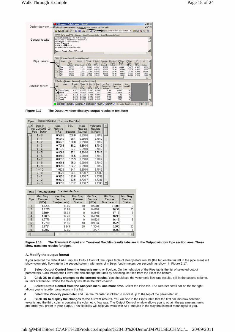
Figure 2.17 The Output window displays output results in text form

Figure 2.18 The Transient Output and Transient Max/Min results tabs are in the Output window Pipe section area. These show transient results for pipes.

A. Modify the output format

If you selected the default AFT Impulse Output Control, the Pipes table of steady-state results (the tab on the far left in the pipe area) will show volumetric flow rate in the second column with units of m3/sec (cubic meters per second), as shown in Figure 2.17.

Ø Select Output Control from the Analysis menu or Toolbar. On the right side of the Pipe tab is the list of selected output parameters. Click Volumetric Flow Rate and change the units by selecting liter/sec from the list at the bottom.

Ø Click OK to display changes to the current results. You should see the volumetric flow rate results, still in the second column, in units of liter/sec. Notice the Velocity results in the third column.

Ø Select Output Control from the Analysis menu one more time. Select the Pipe tab. The Reorder scroll bar on the far right allows you to reorder parameters in the list.

Ø Select the Velocity parameter and use the Reorder scroll bar to move it up to the top of the parameter list.

Ø Click OK to display the changes to the current results. You will see in the Pipes table that the first column now contains velocity and the third column contains the volumetric flow rate. The Output Control window allows you to obtain the parameters, units and order you prefer in your output. This flexibility will help you work with AFT Impulse in the way that is most meaningful to you,



reducing the possibility of errors.

Ø Lastly, double-click the column header Velocity in the Output window Pipes Table. This will open a window in which you can change the units once again if you prefer. These changes are extended to the Output Control parameter data you have previously set.

B. Graph the results

Ø Change to the Graph Results window by choosing it from the Windows menu, Toolbar, pressing Ctrl-G, clicking anywhere on the window if it’s been restored or, if minimized, clicking on the minimized window at the bottom of the Workspace and restoring it. The Graph Results window offers full-featured Windows plot preparation.

Ø Choose Select Graph Data from the View menu or the Toolbar to open the Select Graph Data window (see Figure 2.19). From the All Pipe Stations… list choose pipe 7. Select the Outlet of pipe 7. This is the station connected to the exit valve. A graph of this station shows the pressure and flow histories at the valve.

Figure 2.19 The Select Graph Data window controls the Graph Results content

Ø Click the Add >> button to add this station to the list on the right.

Ø From Graph Parameters select Hydraulic Gradeline (HGL) and choose meters as the Y-Axis units. Then click the Show button to display the graph (Figure 2.20).

This pressure/head history can be compared to that published in Karney, 1992. This is done in the Verifications documentation provided with AFT Impulse.



Figure 2.20 The Graph Results window offers full-featured plot generation.

C. Animate the Results

The animation features in AFT Impulse can greatly aid the understanding of complex transient behavior. Open the Select Graph Data window from the View menu or toolbar again. Select the “Profile Along a Flow Path” tab. There select pipes 1, 6 and 7 from the Pipes List (this is the sequence of pipes from the Supply Tank A at J1 to the discharge valve at J7), select HGL from the Graph Parameters List, and select Animate From Output File option in the Parameter values area (see Figure 2.21). Select the X-Axis Units and HGL Units as meters. Click the Show button.



Figure 2.21 The Select Graph Data window allows selection of animation parameters.

Additional animation control features will be displayed on the Graph Results window (see Figure 2.22). Push the Play button and AFT Impulse will run through all of the results in pipes 1, 6 and 7 for the entire transient which animates the results. The animation can be paused or stopped, and the time can be reset to any desired time using the time slider. If the animation is too fast, slow it down using the animation speed control at the right.

Figure 2.22 The Graph Results window allows animation of output to be displayed. This is the animation shown at 8.1 seconds.

D. View the Visual Report

Ø Change to the Visual Report window by choosing it from the Window menu, Toolbar, pressing Ctrl-I, clicking anywhere on the window if it’s been restored or, if minimized, clicking on the minimized window at the bottom of the Workspace and restoring it. This window allows you to integrate your text results with the graphic layout of your pipe network.

Ø Click the Visual Report Control button on the Toolbar (or View menu) and open the Visual Report Control window, shown in Figure 2.23. Default parameters are already selected, but you can modify these as desired. For now, select Max Pressure Stagnation and Min Pressure Stagnation in the Pipe Results area. Click the Show button. The Visual Report window graphic is generated (see Figure 2.24).



Figure 2.23 The Visual Report Control window selects content for the Visual Report window

It is common for the text in the Visual Report window to overlap when first generated. You can change this by selecting smaller fonts or by dragging the text to a new area to increase clarity (this has already been done in Figure 2.24 as has the selection to show units in a legend). This window can be printed, copied to the clipboard for import into other Windows graphics programs, or saved to file.

Figure 2.24 The Visual Report window integrates results with the model layout

Conclusion

You have now used AFT Impulse's five Primary Windows to build a simple model.



Related Topics

FAQ - Frequently Asked Questions

Primary Window Overview

Pipes and Junctions

Using the Checklist

Steady-State Network Solution Method

Transient Solution Method

The bundle of tools at the left of the Workspace window that allow you to create or select pipes and junctions.

AFT Impulse in fact has two Solvers. The first is called the Steady-State Solver, which as its name suggests obtains a steady-state solution to the pipe network. The second Solver is called the Transient Solver. This solves the waterhammer equations.


The part of AFT Impulse that applies the governing stead-state incompressible flow equations to obtain a steady flow solution to the pipe system.

The part of AFT Impulse that applies the uses the Method of Characteristics to solve the waterhammer equations to obtain a transient solution of the pipe system.





The bar that runs along the bottom of the AFT Impulse window. It shows the status of all Checklist items and the Model Status light.

The light at the left of the Status Bar located at the bottom of the AFT Impulse window.

The speed at which a pressure disturbance propagates through a pipe. The wavespeed depends on the liquid acoustic velocity, the pipe diameter and physical properties, and method of pipe support. Details are given in Wavespeed Mathematical Description.

A solution method for a set of differential equations used to solve the transient waterhammer equations.

Method of Characteristics Mathematical Derivation

The pipe with the fastest end-to-end communication time in a pipe system. Its properties govern the choice of time step. The controlling pipe is identified in the Section Pipes window.

The speed at which a pressure disturbance propagates through a pipe. The wavespeed depends on the liquid acoustic velocity, the pipe diameter and physical properties, and method of pipe support. Details are given in Wavespeed Mathematical Description.





The part of AFT Impulse that applies the uses the Method of Characteristics to solve the waterhammer equations to obtain a transient



solution of the pipe system.


A variant case of a model that is created in the Scenario Manager.



Impulse

Documents

Transcript of Impulse