
Improving wheel Speed Sensing and...
60
ISSN 0280-5316 ISRN LUTFD2/TFRT--5716--SE Improving wheel Speed Sensing and Estimation Christian Trobro Mathias Magnusson Department of Automatic Control Lund Institute of Technology December 2003
Transcript of Improving wheel Speed Sensing and...

ISSN 0280-5316 ISRN LUTFD2/TFRT--5716--SE
Improving wheel Speed Sensing and Estimation
Christian Trobro Mathias Magnusson
Department of Automatic Control Lund Institute of Technology
December 2003

Document name MASTER THESIS Date of issue December 2003
Department of Automatic Control Lund Institute of Technology Box 118 SE-221 00 Lund Sweden Document Number
ISRN LUTFD2/TFRT--5716--SE Supervisor Ola Nockhammar, Haldex. Anders Rantzer, LTH
Author(s) Christian Trobro and Mathias Magnusson
Sponsoring organization
Title and subtitle Improving wheel Speed Sensing and Estimation. (Förbättring av hjulhastighetsmätning och estimering).
Abstract This master thesis project commissioned by Haldex Brake Products AB (in Landskrona, Sweden), and in association with the Department of Automatic Control, Lund Institute of Technology, deals with the problem of correct wheel speed measurements. Investigation into different types of sensors, Inductive-, Hall Effect- and Magneto-Resistive sensors have been carried out, which are sensors that may be used, when measuring the velocity of a wheel. It also looks into different types of methods that can be used to estimate a velocity; zero detection, estimation with few measurements, and tracking demodulation. Problems, such as noise, time demanding calculations and adapting the sensor signal so it may be used in a microcontroller, which could arise when implementing these methods into a microcontroller, are also investigated. The conclusions are that to obtain wheel speed estimates at low speed sufficiently fast, the information in the sinusoidal signal from the sensors has to be used, and therefore, if one sensor is used, the Few Measurements method is the most appropriate, and if two sensors are used the Tracking Demodulation method. Finally scheduling is suggested, which means that the normal zero detection is used at high speed and the tracking demodulation method is used at low speed.
Keywords
Classification system and/or index terms (if any)
Supplementary bibliographical information ISSN and key title 0280-5316
ISBN
Language English
Number of pages 58
Security classification
Recipient’s notes
The report may be ordered from the Department of Automatic Control or borrowed through: University Library 2, Box 3, SE-221 00 Lund, Sweden Fax +46 46 222 44 22 E-mail [email protected]

Improving wheel speed sensing
and estimation
Master Thesis Students: Supervisor Haldex Brake Products AB: Mathias Magnusson, E98 Ola Nockhammar Christian Trobro, E01 Supervisor Lund University (LTH):
Anders Rantzer Department of Automatic Control

Table of Content
1
Table of Content
1. Introduction...........................................................................3
2. The use of wheel speed measurement in an ABS ..............5
2.1. ABS system ...............................................................................5
3. Sensors ..................................................................................7
3.1. Velocity measurement.................................................................7
3.2. Working principles of Inductive sensors........................................7
3.3. Working principles of Solid-state sensors......................................10
3.3.1. Main idea.........................................................................10
3.3.2. Hall-effect sensor ................................................................11
3.3.3. Magneto resistive sensor........................................................13
3.4. Summary .........................................................................................13
4. The Sensor signal ..................................................................14
4.1. Waveform characteristics..........................................................14
4.2. Embedded Signal processing.....................................................16
4.3. Summary...........................................................................................17
5. Different velocity measurement methods ............................18
5.1. Using one sensor .....................................................................18
5.1.1. Frequency estimating using zero detection....................................18
5.1.2. Few Measurements method ....................................................21
5.2. Using two sensors ...................................................................25
5.2.1. Tracking Demodulation method .................................................25
5.3. Tracking Demodulation- vs. Few Measurements methods...............31
5.4. Summary...........................................................................................33
Table of Content
2
6. Noise influence on- and filtering of the sensor signal
and the frequency estimations............................................34
6.1. Filtering the analogue sensor signal ..........................................34
6.2. The Wobble disturbance ...........................................................36
6.3. ARMA-filters ...........................................................................37
6.3.1. AR-filter ..........................................................................37
6.3.2. MA-filter ..........................................................................37
6.4. Summary .........................................................................................38
7. Real sensor testing ................................................................39
8. Implementation methods into a micro controller ................41
8.1. The micro controller..................................................................41
8.2. Pre-signal processing for Inductive sensors..................................41
8.3. General implementation ideas ...................................................43
8.4. Implementation of Few Measurements method .............................44
8.5. Implementation of Hall-Effect sensor measurement .......................47
8.6. Summary...........................................................................................49
9. Conclusions ...........................................................................50
Appendix .......................................................................................52
A. Wheel velocity............................................................................52
B. Deriving from Frequency Estimation from Few Measurements............53
References.....................................................................................54
Introduction
3
1. Introduction
In today’s automotive systems (such as ABS, ESP etc.), it is of great
importance to have well defined and reliable wheel speed signals. Therefore it
is very convenient that the sensors, which measure these signals, are robust.
This has resulted in sensors with a rather rough resolution, which has been
enough in traditional “Bang-Bang” ABS-systems. To make improvements in
these systems, much better wheel speed signals are needed. In future
systems the intelligence will be moved closer to the wheels, which makes
better use of the sensor signals.
This master thesis project commissioned by Haldex Brake Products AB (in
Landskrona, Sweden), deals with an investigation whether it is possible to
make the present signals from the sensors better? E.g. at low vehicle speed,
the today’s sensor signal is too weak, and therefore no reliable velocity
estimation can be performed. Is it possible to use other wheel speed
estimation methods? Is it achievable to make improvements with more
advanced signal processing? Is another sensor needed to achieve
improvements? Could two sensors be used to obtain better results?
In chapter two the wheel speed sensor in an Anti-Lock Braking System is
presented, or more exactly; how this sensor signal is used in an ABS. In the
third chapter the general function of wheel speed sensing with a sensor is
introduced, and also different kinds of sensors are discussed, and their
advantages and disadvantages are shown. The characteristic of the waveform
in the sensor signal is brought up in chapter four. In the following chapter,
i.e. chapter five, different wheel speed estimation methods, i.e. common zero
detection, few measurements method and tracking demodulation method,
are introduced. The working principle of these methods, and their
advantages and disadvantages are discussed and analyzed. In chapter six
disturbances on the attained signals and estimations are lightened, and
suggested filtering of these disturbances are introduced. The test rig, on
which the estimation methods have been tested, is presented in chapter

Introduction
4
seven. In chapter eight, the general implementation ideas of the different
estimation methods are discussed and shown. Finally, in chapter nine, the
conclusions of this project are presented and summarized.
The use of wheel speed measurement in an ABS
5
2. The use of wheel speed measurement in an ABS
The following chapter will investigate how the wheel speed measurement is
used in an ABS (Anti-Lock Braking System)1, and the importance of this
speed measurement to be reliable.
2.1. ABS system
A main function of the ABS is to keep the brakes from being jammed. A main
idea is to release pressure from the brakes when they are locked up. To
control this, a measurement called slip is made. The slip is defined as the
relative difference of the circumferential velocity of the driven wheel, wwrω
and its absolute velocity wv . This gives following statement for the slip2:
w
www
v
vrs
−=
ω (2.1)
The wheel speed wv may be calculated from the velocity from the two non-
driven wheels, assuming that the vehicle has two front wheel drive. This
means when the friction slip is -1, the front brakes are locked and the front
wheels skid on the surface, a situation that an ABS system will prevent from
happening.
A modern antilock brake system is an electronic feedback controller system,
which uses the information about the slip to control the brake pressure
applied to the brakes. These systems often consist of a sensor that measures
the circumferential speed of the wheels. It also consists of an electronic
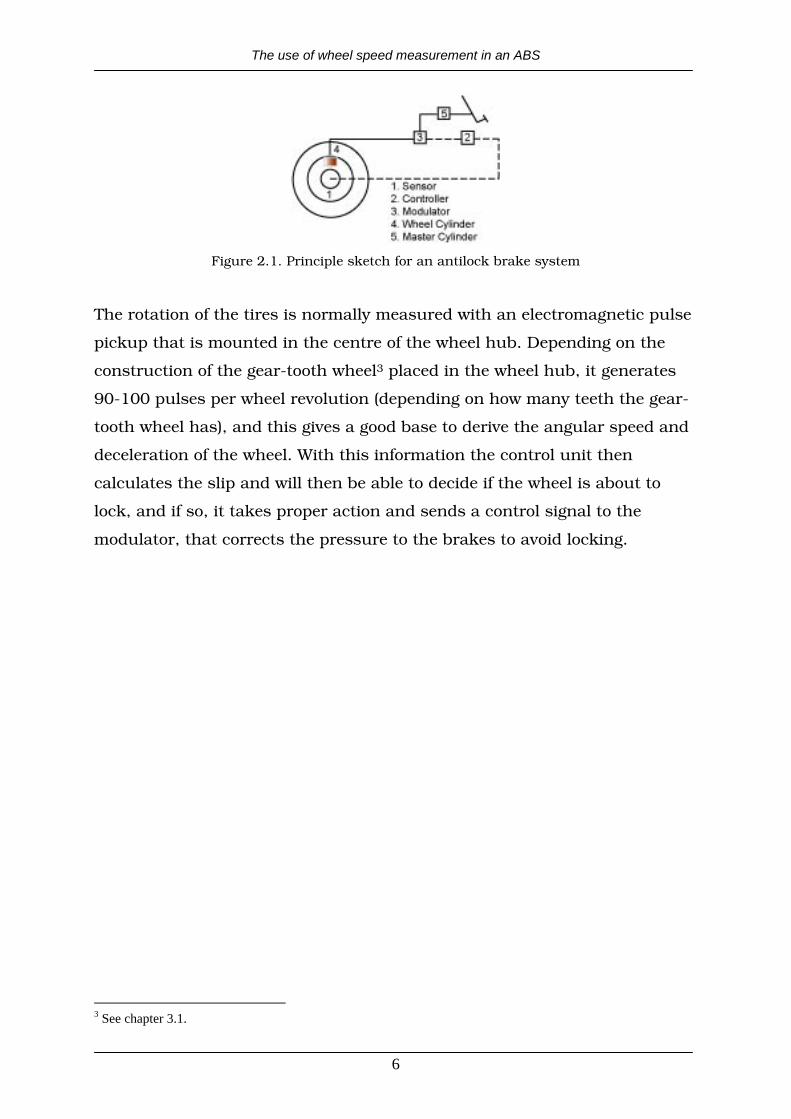
control unit and a pressure modulator to control the brakes. See figure 2.1
for a principle sketch.
1 For further information see reference [12] and [14]. 2 For further information see reference [14].
The use of wheel speed measurement in an ABS
6
Figure 2.1. Principle sketch for an antilock brake system
The rotation of the tires is normally measured with an electromagnetic pulse
pickup that is mounted in the centre of the wheel hub. Depending on the
construction of the gear-tooth wheel3 placed in the wheel hub, it generates
90-100 pulses per wheel revolution (depending on how many teeth the gear-
tooth wheel has), and this gives a good base to derive the angular speed and
deceleration of the wheel. With this information the control unit then
calculates the slip and will then be able to decide if the wheel is about to
lock, and if so, it takes proper action and sends a control signal to the
modulator, that corrects the pressure to the brakes to avoid locking.
3 See chapter 3.1.
Sensors
7
3. Sensors
This chapter brings up the principle for common velocity measurements with
a sensor and a gear-tooth wheel, and also discuss how the signals are
obtained in different types of sensors.
3.1. Velocity measurement
The idea when measuring the velocity of a vehicle is that a gear-tooth wheel
(also called target wheel) and a sensor are applied on each of the vehicle
wheels. The gear-tooth wheel is of ferromagnetic material. When the wheel is
moving, the sensor is able to “feel” the changes of the magnetic field between
the target wheel and a permanent magnet in the sensor. The sensor is
detecting and transforming the variation in flux level to an output voltage.
The frequency of this output voltage is proportional to the wheel frequency.
How this signal is obtained differs between different types of sensors. In this
and the following chapter the main idea for Inductive-, Hall-Effect- and
Magneto-Resistive sensors are discussed.
3.2. Working principles of Inductive sensors
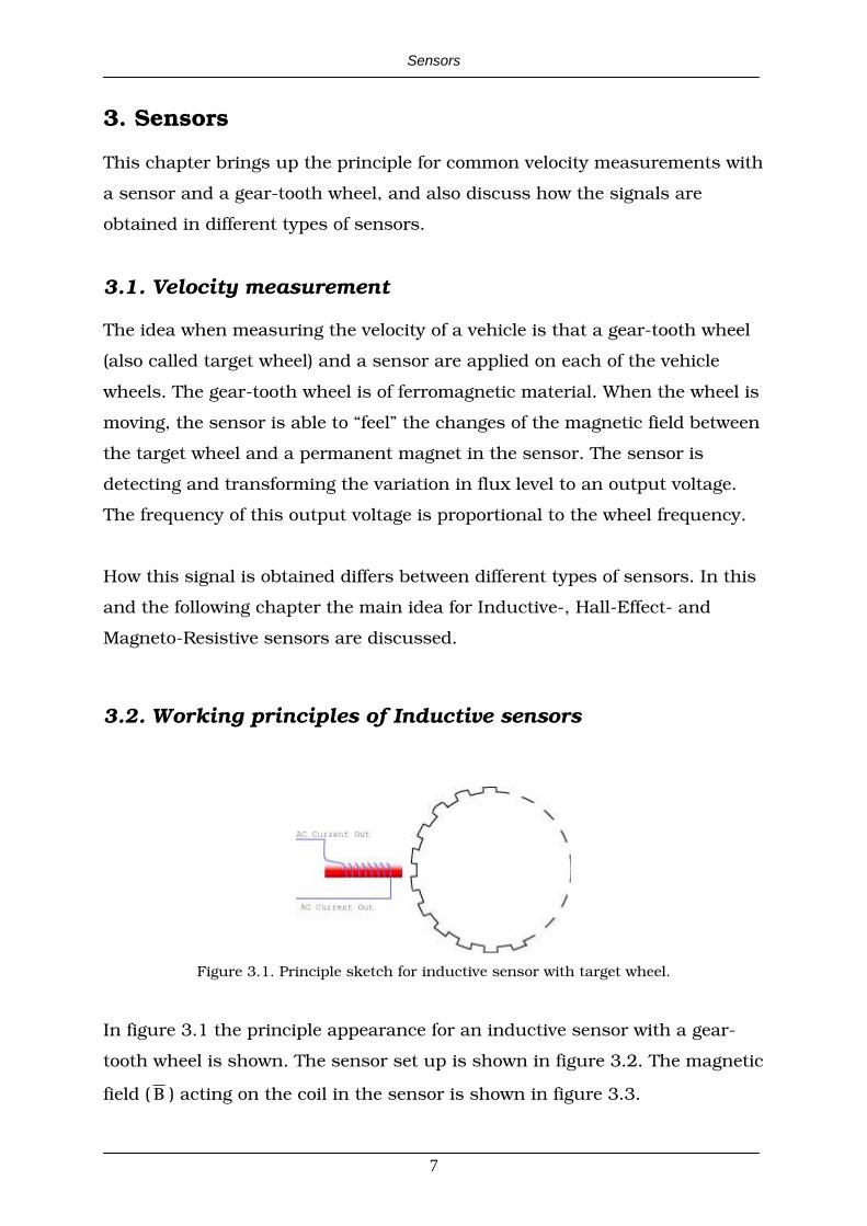
Figure 3.1. Principle sketch for inductive sensor with target wheel.
In figure 3.1 the principle appearance for an inductive sensor with a gear-
tooth wheel is shown. The sensor set up is shown in figure 3.2. The magnetic
field ( Β ) acting on the coil in the sensor is shown in figure 3.3.

Sensors
8
Figure 3.2. Sensor setup in proportion to the target wheel
Figure 3.3. Magnetic field acting on the coil
The output voltage from the sensor is given by
( ) −===
N
1iidt
d
dt
dte (3.1)
where Ψ is the total flux linkage and iϕ is the flux linkage in one of the N
windings of the coil. Neglecting the flux leakage, the uniform flux linkage �
in the magnetic core is
( )==A
i dB (3.2)
where A is the cross section of the core. If the core is rectangular with length
L in the y-direction, then
( )( )
( )+⋅=
�t
�
t�
dRBL (3.3)
where ( )t is the location of the target wheel at time t when it is above the

Sensors
9
core, � is the width of the core in the � -direction and R is the radius of the
target wheel. Eq. (3.1) – (3.3) give
( ) ( )( )
( )( )
( )
( )++
⋅−=⋅−=�
t�
t�
�t
�
t�
dBd
d
dt
dNLRdB
dt
dNLRte (3.4)
If the wheel has constant velocity, i.e. dt
d = then
( ) ( ) ( ) ( )[ ]( )
( )+−+−=⋅−=
�t
�
t�
BBNLRdBd
dNLRte (3.5)
From this equation it is seen that the amplitude of the voltage is proportional
to the velocity of the wheel4. Therefore a weaker signal (lower SNR5) for small
velocities for the Inductive sensor is given. This results in the need of some
sort of filtering and amplification of the signal, before velocity estimation can
be performed. Also it says from eq. (3.5) that the amplitude becomes large for
high velocities. To show that eq. (3.5) is valid the test rig6 has been run with
an inductive sensor at different velocities. See figures 3.4.
Figure 3.4a. Sensor frequency at 100Hz. Figure 3.4b. Sensor frequency at 150Hz.
4 See reference [6]. 5 SNR=Signal to noise ratio 6 Information about the test rig is presented in chapter 7.
Sensors
10
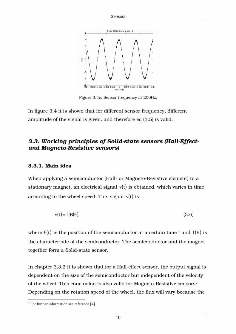
Figure 3.4c. Sensor frequency at 200Hz.
In figure 3.4 it is shown that for different sensor frequency, different
amplitude of the signal is given, and therefore eq (3.5) is valid.
3.3. Working principles of Solid-state sensors (Hall-Effect- and Magneto-Resistive sensors)
3.3.1. Main idea
When applying a semiconductor (Hall- or Magneto-Resistive element) to a
stationary magnet, an electrical signal ( )tv is obtained, which varies in time
according to the wheel speed. This signal ( )tv is
( ) ( )[ ]Bftv = (3.6)
where ( )t is the position of the semiconductor at a certain time t and ( )Bf is
the characteristic of the semiconductor. The semiconductor and the magnet
together form a Solid-state sensor.
In chapter 3.3.2 it is shown that for a Hall-effect sensor, the output signal is
dependent on the size of the semiconductor but independent of the velocity
of the wheel. This conclusion is also valid for Magneto-Resistive sensors7.
Depending on the rotation speed of the wheel, the flux will vary because the 7 For further information see reference [4].
Sensors
11
magnetic field will bend different ways, due to the position on the target
wheel. Bending characteristics of the magnetic field also occurs when the
wheel is stationary. The magnet generates a stationary flux, which provides
an output signal on the sensors; due to the fact that the sensor needs a
supply voltage to be able perform a signal. Therefore it is possible to measure
very slow velocities. (Inductive sensors can only measure the variations in
the flux and are therefore unable to perform reliable output signals for low
velocities).
3.3.2. Hall-effect sensor
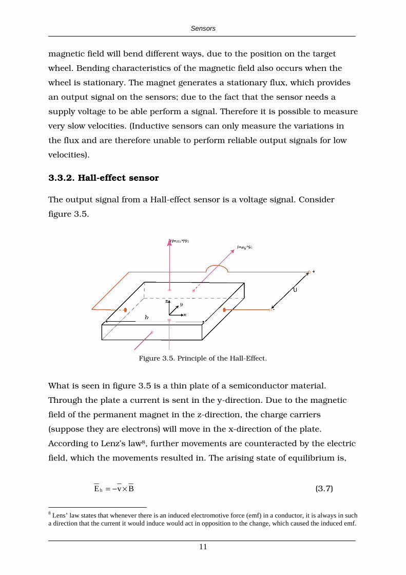
The output signal from a Hall-effect sensor is a voltage signal. Consider
figure 3.5.
Figure 3.5. Principle of the Hall-Effect.
What is seen in figure 3.5 is a thin plate of a semiconductor material.
Through the plate a current is sent in the y-direction. Due to the magnetic
field of the permanent magnet in the z-direction, the charge carriers
(suppose they are electrons) will move in the x-direction of the plate.
According to Lenz’s law8, further movements are counteracted by the electric
field, which the movements resulted in. The arising state of equilibrium is,
BvEh ×−= (3.7)
8 Lens’ law states that whenever there is an induced electromotive force (emf) in a conductor, it is always in such a direction that the current it would induce would act in opposition to the change, which caused the induced emf.

Sensors
12
where hE is the electrical field, v is the velocity of the charge carriers and B
is the magnetic field. From figure 3.4 it is seen that the velocity of the
electrons is
0y vev ⋅−= (3.8)
and the electrical field is then
00x0z0yh BveBe)ve(E =×−−= (3.9)
The Hall voltage over the plate is given by9
bBvdxEV 00
b
0
hh =−= (3.10)
where b is the width of the plate. In eq. (3.10) it is shown that the output
voltage is dependent on the size of the semi-conductor, and the amplitude of
the output signal is independent of the wheel speed10, as stated before.
The current I through the plate can be written as
vqnI ⋅⋅= (3.11)
where n is the number of free charge carriers q per volume unit, which move
through the plate. The ratio
qn
1
BI
E
zy
x
⋅=
⋅ (3.12)
is called the Hall coefficient11 and is different for different materials, i.e.
different sensors. This means that the output is different for different types 9 See reference [3]. 10 See reference [6]. 11 See reference [3].
Sensors
13
of sensors (and slightly differ from sensor to sensor). Therefore when, for
instance two Hall Effect sensors are used in a wheel speed measurement, the
amplitude of the sensor signals could differ, which could cause problems in
the wheel speed estimation.
3.3.3. Magneto resistive sensor
Due to the magneto resistive effect12, resistance variation may be measured
in a Magneto resistive sensor. Depending on the rotation speed of the wheel,
the resistivity will vary proportional to the wheel speed. Note that the
amplitude of the output signal is independent to the wheel speed. With a
Magneto-Resistive sensor, larger output signals are achieved (larger SNR)
compared to a Hall-Effect- or an Inductive sensor13. On the market there are
companies which have been doing research on magneto-resistive sensors,
but have not come to a final solution. Therefore further investigation on the
Magneto-Resistive sensor is not done in this rapport.
3.4 Summary
In this chapter it is shown that the amplitude of the inductive sensor signal
is proportional to the wheel speed, which means that the SNR becomes low
at slow wheel speed. The signal of the Solid-State sensors is instead
independent of the wheel speed, which means more reliable signals are
obtained at low velocities.
12 The property of a current carrying a magnetic material to change its resistivity, in the presence of an external magnetic field. 13 See reference [4].
The Sensor signal
14
4. The Sensor signal
The characteristics of the sensor signal for different appearance of the target
wheel, and a discussion of embedded signal processing in common Solid-
State sensors, are brought up in this chapter.
4.1. Waveform characteristics
The appearance of the output signal of the different sensors has some factors
in common, but also some differences. In this chapter these factors are
discussed.
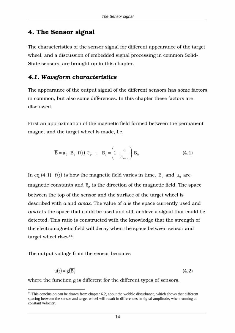
First an approximation of the magnetic field formed between the permanent
magnet and the target wheel is made, i.e.
( ) 0max
110 Ba
a1B,etfB ⋅−=⋅⋅⋅= ϕ (4.1)
In eq (4.1), ( )tf is how the magnetic field varies in time. 0B and 0 are
magnetic constants and ϕe is the direction of the magnetic field. The space
between the top of the sensor and the surface of the target wheel is
described with a and amax. The value of a is the space currently used and
amax is the space that could be used and still achieve a signal that could be
detected. This ratio is constructed with the knowledge that the strength of
the electromagnetic field will decay when the space between sensor and
target wheel rises14.
The output voltage from the sensor becomes
( ) ( )Bgtu = (4.2)
where the function g is different for the different types of sensors.
14 This conclusion can be drawn from chapter 6.2, about the wobble disturbance, which shows that different spacing between the sensor and target wheel will result in differences in signal amplitude, when running at constant velocity.

The Sensor signal
15
Conclusion of the output waveform is made15, i.e. the function f from eq.
(4.1) will be dependent on the angular velocity of the wheel and the geometry
of the target wheel, such as space between teeth on the wheel, width and
appearance of the teeth. How the output voltage will be affected by different
constructing parameters of the target wheel is shown in figure 4.1.
Figure 4.1a. Even spacing and even teeth. Figure 4.1b. Large spacing, even teeth.
c
Figure 4.1c. Large spacing, narrow teeth
In figure 4.1a it is shown that with an even width and gap between the teeth,
a sinusoidal output waveform is given.
As seen in figure 4.1b an increased gap between the teeth results in an
exponential raise and fall of the output waveform. The output waveform has
its maximum around the middle of each tooth and its minimum value in the
middle between the teeth. For the Inductive sensor the maximum amplitude
is still dependent on the angular velocity.
15 See reference [2]
a b
The Sensor signal
16
As seen in figure 4.1c, a narrow tooth with large spacing between each
following tooth will decrease the raise/fall time in the waveform, and also
shorten the signals negative output value after a tooth has past.
In chapter 5 different estimation methods of the wheel speed are discussed.
Some of the methods are based on different waveforms of the sensor signal.
Therefore the construction of the target wheel is important.
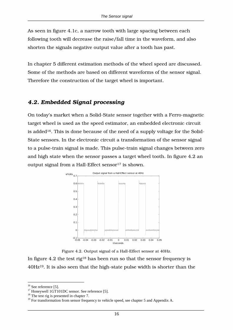
4.2. Embedded Signal processing
On today’s market when a Solid-State sensor together with a Ferro-magnetic
target wheel is used as the speed estimator, an embedded electronic circuit
is added16. This is done because of the need of a supply voltage for the Solid-
State sensors. In the electronic circuit a transformation of the sensor signal
to a pulse-train signal is made. This pulse-train signal changes between zero
and high state when the sensor passes a target wheel tooth. In figure 4.2 an
output signal from a Hall-Effect sensor17 is shown.
-0.05 -0.04 -0.03 -0.02 -0.01 0 0.01 0.02 0.03 0.04 0.05-0.1
0
0.1
0.2
0.3
0.4
0.5
0.6
0.7
t/seconds
v/Volts Output signal from a Hall-Effect sensor at 40Hz
Figure 4.2. Output signal of a Hall-Effect sensor at 40Hz.
In figure 4.2 the test rig18 has been run so that the sensor frequency is
40Hz19. It is also seen that the high-state pulse width is shorter than the
16 See reference [5]. 17 Honeywell 1GT101DC sensor. See reference [5]. 18 The test rig is presented in chapter 7. 19 For transformation from sensor frequency to vehicle speed, see chapter 5 and Appendix A.

The Sensor signal
17
lower state, because the target wheel on the test rig has got larger space
than teeth, see figure 4.1b.
An advantage with the pulse modulator circuit is that more reliable wheel
speed estimations can be made. The velocity estimation is made by
measuring time in between two rising flanks, i.e. the period time of the
sensor signal. A problem occurs when driving at low speed. If there are time
demands on the velocity estimator, i.e. a new estimated wheel speed has to
be made within a defined time. Then if the period time of the sensor signal is
more than the demanded estimation time, this will result in missed
deadlines. For instance, the fastest estimation time for the wheel speed in
the example in figure 4.2 is around 25ms. That is one of the reasons why
another estimation procedure is needed for low speed.
4.3 Summary
Different waveform characteristics are achieved by the sensors for different
appearances of the target wheel. To obtain a sinusoidal signal even spacing
between teeth and gaps are needed, which is appropriate for the estimation
methods described in chapter 5. (See footnote nr. 20.)
Common Solid-State sensors have embedded signal processing, due to their
need of a supply voltage. This signal processing transforms the signal to a
pulse-train, and therefore a more reliable output signal is achieved. At low
velocities a problem occurs, which is that its velocity estimation procedure
cannot perform a new estimate if there are time demands on it. Therefore the
original sensor (without embedded signal processing) is needed, to estimate
wheel speeds at low velocities more often.
20 More exactly, Few Measurements- and Tracking Demodulation method.

Different velocity measurement methods
18
5. Different velocity measurement methods
In this chapter different wheel speed estimation methods are discussed and
analyzed. These methods are zero-detection, few measurements method and
tracking demodulation method, where the first two methods use one sensor,
and the last uses two sensors to estimate the velocity. But first a clarification
of how much a sensor frequency is in vehicle speed.
The frequency of the sensor signal is, as mentioned, proportional to the
wheel speed. When determining the speed of the vehicle, a transformation
from the frequency of the sensor has to be made. Assuming the sensor
frequency is sf , the vehicle speed is vv , the number of teeth on the target
wheel is N, the vehicle wheel radius vr and the vehicle wheel circumference
is vo . The vehicle speed is then
ssv
sv
v fkfN
r�2f
No
v ⋅=⋅⋅⋅
=⋅= (5.1)
If 0.5mrv = and 96N = the transformation factor k equals m2103.3 −⋅ . (See
footnote nr. 21). In this chapter, step responses in sensor frequency are
investigated. To understand in which vehicle speed range the step responses
take place, see Table A.I in Appendix A.
5.1. Using one sensor
5.1.1. Frequency estimating using zero detection
When simulating with a normal sinusoidal it is easy to calculate the
frequency by detecting every zero crossing, and calculating the time in-
between zeroes. This is actually how the velocity estimation is done in
21An approximation of the radius of a truck wheel is 0.5m, and the number of teeth on the target wheel of Haldex Brake Products is 96.
Different velocity measurement methods
19
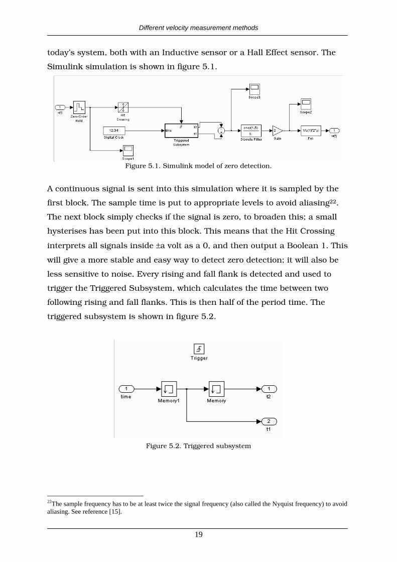
today’s system, both with an Inductive sensor or a Hall Effect sensor. The
Simulink simulation is shown in figure 5.1.
Figure 5.1. Simulink model of zero detection.
A continuous signal is sent into this simulation where it is sampled by the
first block. The sample time is put to appropriate levels to avoid aliasing22.
The next block simply checks if the signal is zero, to broaden this; a small
hysterises has been put into this block. This means that the Hit Crossing
interprets all signals inside ±a volt as a 0, and then output a Boolean 1. This
will give a more stable and easy way to detect zero detection; it will also be
less sensitive to noise. Every rising and fall flank is detected and used to
trigger the Triggered Subsystem, which calculates the time between two
following rising and fall flanks. This is then half of the period time. The
triggered subsystem is shown in figure 5.2.
Figure 5.2. Triggered subsystem
22The sample frequency has to be at least twice the signal frequency (also called the Nyquist frequency) to avoid aliasing. See reference [15].
Different velocity measurement methods
20
To give a more stable value of the frequency, a mean value of measured half
period times are read, and then a value of the frequency is calculated.
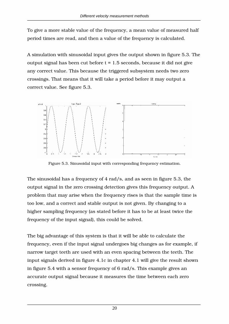
A simulation with sinusoidal input gives the output shown in figure 5.3. The
output signal has been cut before t = 1.5 seconds, because it did not give
any correct value. This because the triggered subsystem needs two zero
crossings. That means that it will take a period before it may output a
correct value. See figure 5.3.
Figure 5.3. Sinusoidal input with corresponding frequency estimation.
The sinusoidal has a frequency of 4 rad/s, and as seen in figure 5.3, the
output signal in the zero crossing detection gives this frequency output. A
problem that may arise when the frequency rises is that the sample time is
too low, and a correct and stable output is not given. By changing to a
higher sampling frequency (as stated before it has to be at least twice the
frequency of the input signal), this could be solved.
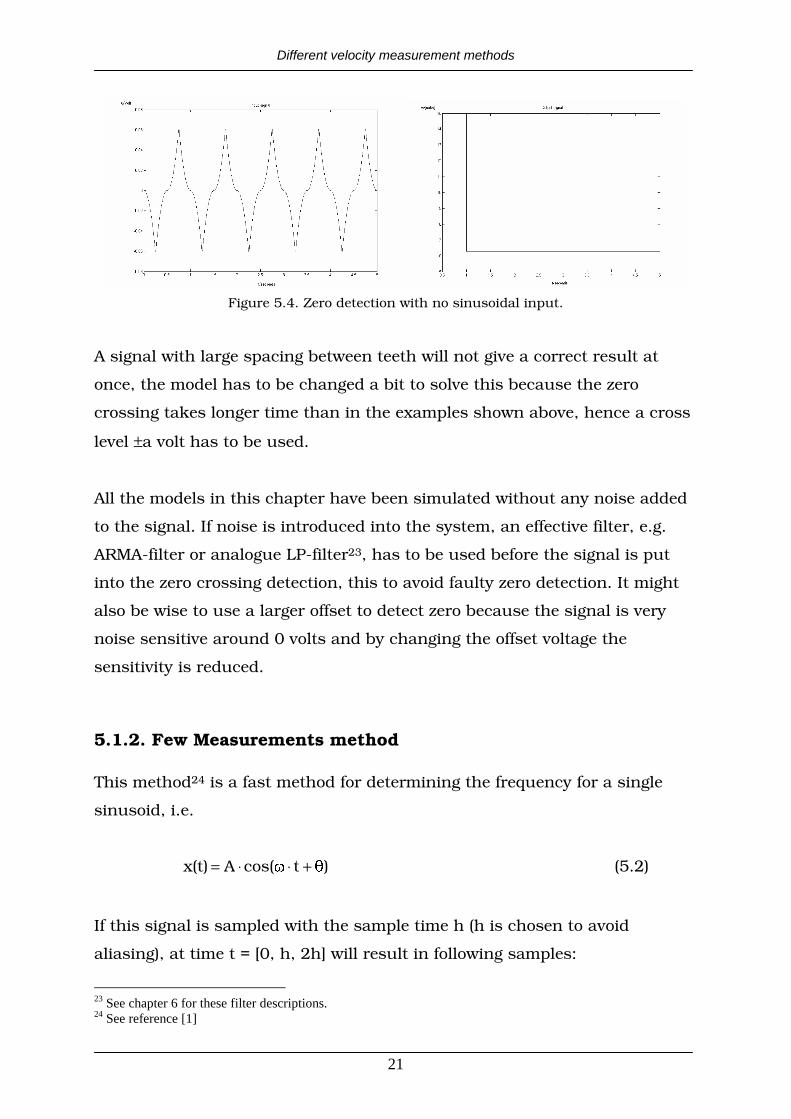
The big advantage of this system is that it will be able to calculate the
frequency, even if the input signal undergoes big changes as for example, if
narrow target teeth are used with an even spacing between the teeth. The
input signals derived in figure 4.1c in chapter 4.1 will give the result shown
in figure 5.4 with a sensor frequency of 6 rad/s. This example gives an
accurate output signal because it measures the time between each zero
crossing.
Different velocity measurement methods
21
Figure 5.4. Zero detection with no sinusoidal input.
A signal with large spacing between teeth will not give a correct result at
once, the model has to be changed a bit to solve this because the zero
crossing takes longer time than in the examples shown above, hence a cross
level ±a volt has to be used.
All the models in this chapter have been simulated without any noise added
to the signal. If noise is introduced into the system, an effective filter, e.g.
ARMA-filter or analogue LP-filter23, has to be used before the signal is put
into the zero crossing detection, this to avoid faulty zero detection. It might
also be wise to use a larger offset to detect zero because the signal is very
noise sensitive around 0 volts and by changing the offset voltage the
sensitivity is reduced.
5.1.2. Few Measurements method
This method24 is a fast method for determining the frequency for a single
sinusoid, i.e.
�)tcos(�Ax(t) +⋅⋅= (5.2)
If this signal is sampled with the sample time h (h is chosen to avoid
aliasing), at time t = [0, h, 2h] will result in following samples:
23 See chapter 6 for these filter descriptions. 24 See reference [1]
Different velocity measurement methods
22
[ ] ( )[ ] ( )[ ] ( )h2cosA2x
hcosA1x
cosA0x
+⋅⋅⋅=+⋅⋅=
⋅= (5.3)
If
[ ] [ ][ ]1x2
2x0xr
⋅+= (5.4)
and using the trigonometrically equations
( ) ( ) ( ) ( ) ( )
( )−⋅=⋅⋅=⋅
⋅−⋅=+
1acos2cos(a)
cos(a)sin(a)2a)sin(2
bsinasinbcosacosbacos
2
(5.5)
it can be shown that25
( )hcosr ⋅= (5.6)
It can be seen when eq. (5.4) is analyzed small values of x[1], i.e. close to
zero, small disturbances have large effect and the estimate of r becomes too
high. Compensation can be made for this problem by adding zero-crossing
detection, which means no sampling takes place close to zero. Another
problem is if � is small, which can give an over-sampled signal if h has such
a value that it takes more than 12 samples per period. This will result in that
r is close to the absolute value 1, and this error could give values outside the
range of cosine [ ]1 1,- + . A problem like this can be solved by changing the
sample rate for different � , so the three samples are taken during a quarter
of the period of the signal.
25 For proof, see appendix B.1.
Different velocity measurement methods
23
An alternative with Few Measurement is to use one more sample x[3] and
compute two cosine estimates26, i.e.
[ ] [ ][ ]
[ ] [ ][ ]2x2
3x1xr ;
1x2
2x0xr 21 ⋅
+=⋅+= (5.7)
which are not statistically independent and their variances and covariance
are
[ ]( ) [ ]( ) [ ] [ ]2x1x
r ;
2x
)r(0,5 ;
1x
)r(0,5 2
122
222
22
222
1 ⋅⋅−=⋅+=⋅+= (5.8)27
To estimate r, a weighted average is made, i.e.
.b anda where,ba
rbrar 12
2112
22
21 −=−=+
⋅+⋅= (5.9)
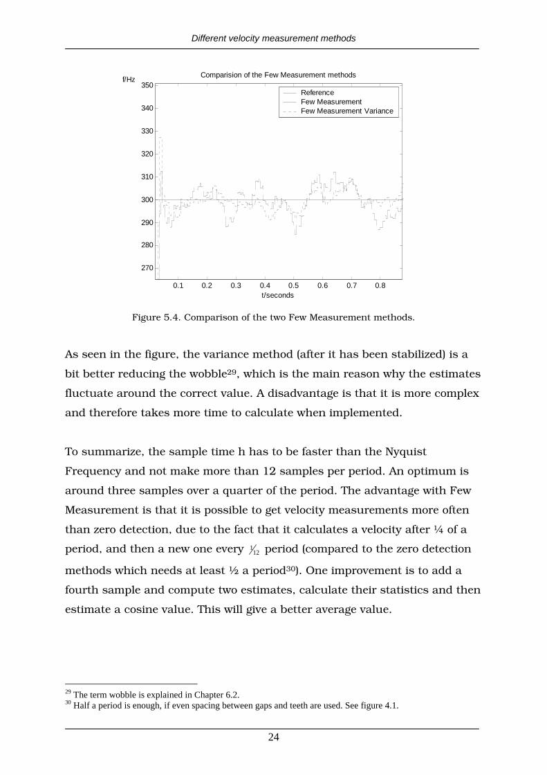
A comparison of these two methods has been run in Simulink and the result
is shown in figure 5.4. Real sensor data from an inductive sensor has been
used as input data. The frequency on the test rig28 is 300Hz and a frequency
estimate is produced every fifth millisecond. This estimate is an average of
all the moment values calculated during the last five milliseconds.
26 See reference [1]. 27 For variances and covariance estimations see reference [1]. 28 Further about the test rig in chapter 7.
Different velocity measurement methods
24
0.1 0.2 0.3 0.4 0.5 0.6 0.7 0.8
270
280
290
300
310
320
330
340
350
t/seconds
f/HzComparision of the Few Measurement methods
ReferenceFew MeasurementFew Measurement Variance
Figure 5.4. Comparison of the two Few Measurement methods.
As seen in the figure, the variance method (after it has been stabilized) is a
bit better reducing the wobble29, which is the main reason why the estimates
fluctuate around the correct value. A disadvantage is that it is more complex
and therefore takes more time to calculate when implemented.
To summarize, the sample time h has to be faster than the Nyquist
Frequency and not make more than 12 samples per period. An optimum is
around three samples over a quarter of the period. The advantage with Few
Measurement is that it is possible to get velocity measurements more often
than zero detection, due to the fact that it calculates a velocity after ¼ of a
period, and then a new one every 121 period (compared to the zero detection
methods which needs at least ½ a period30). One improvement is to add a
fourth sample and compute two estimates, calculate their statistics and then
estimate a cosine value. This will give a better average value.
29 The term wobble is explained in Chapter 6.2. 30 Half a period is enough, if even spacing between gaps and teeth are used. See figure 4.1.
Different velocity measurement methods
25
5.2. Using two sensors
It could be of great interest to investigate whether a good estimate of the
wheel speed can be obtained using two sensors. One way is a method called
“Tracking Demodulation” method31.
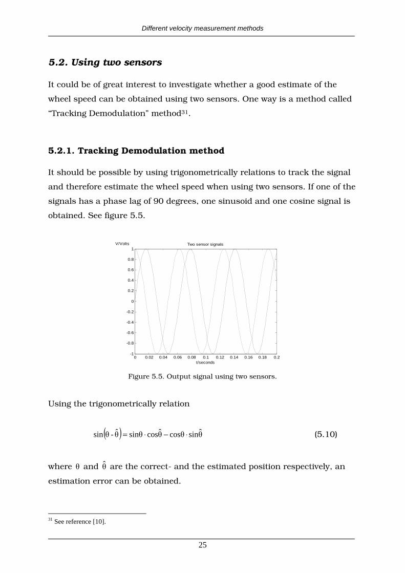
5.2.1. Tracking Demodulation method
It should be possible by using trigonometrically relations to track the signal
and therefore estimate the wheel speed when using two sensors. If one of the
signals has a phase lag of 90 degrees, one sinusoid and one cosine signal is
obtained. See figure 5.5.
0 0.02 0.04 0.06 0.08 0.1 0.12 0.14 0.16 0.18 0.2-1
-0.8
-0.6
-0.4
-0.2
0
0.2
0.4
0.6
0.8
1
t/seconds
V/Volts Two sensor signals
Figure 5.5. Output signal using two sensors.
Using the trigonometrically relation
( ) ˆsincosˆcossinˆ-sin ⋅−⋅= (5.10)
where and ˆ are the correct- and the estimated position respectively, an
estimation error can be obtained.
31 See reference [10].
Different velocity measurement methods
26
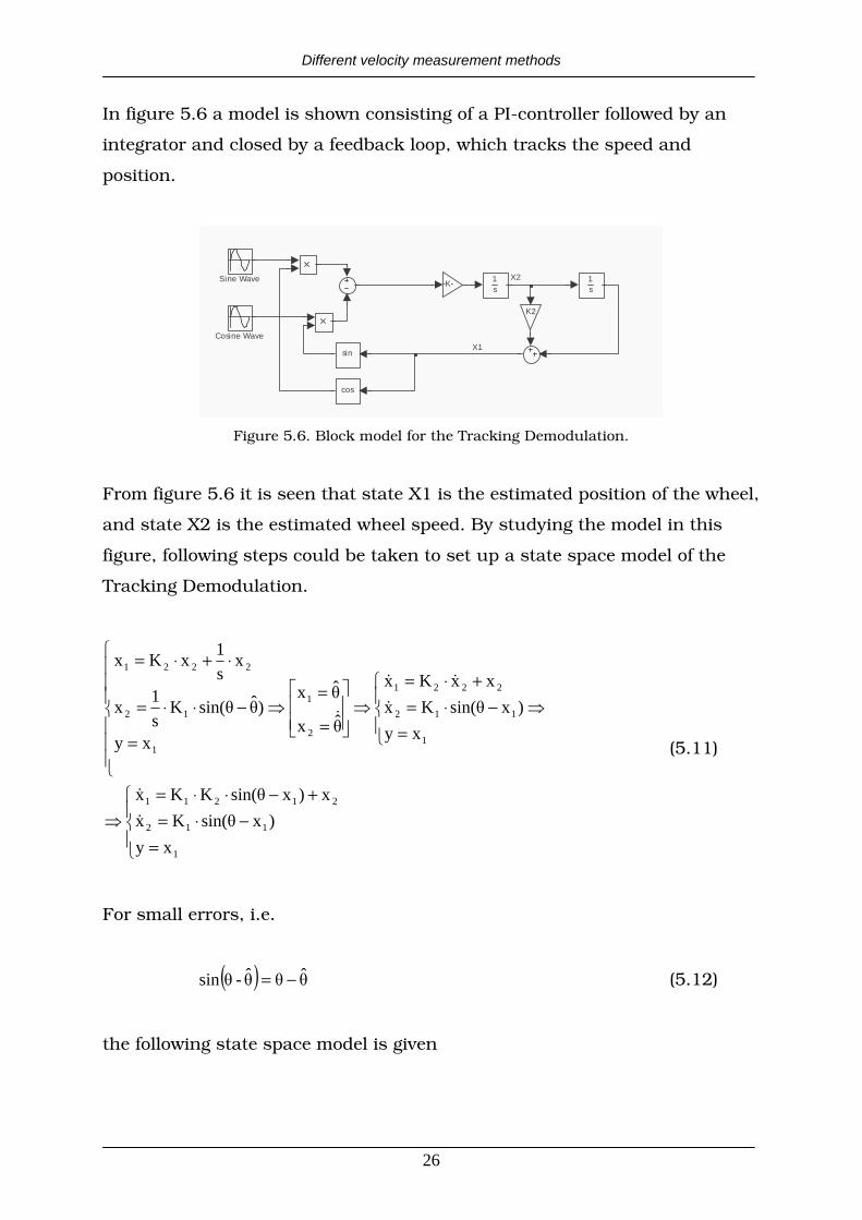
In figure 5.6 a model is shown consisting of a PI-controller followed by an
integrator and closed by a feedback loop, which tracks the speed and
position.
X1
X2
cos
sin
Sine Wave 1s
1s
K2
-K-
Cosine Wave
Figure 5.6. Block model for the Tracking Demodulation.
From figure 5.6 it is seen that state X1 is the estimated position of the wheel,
and state X2 is the estimated wheel speed. By studying the model in this
figure, following steps could be taken to set up a state space model of the
Tracking Demodulation.
=−⋅=
+−⋅⋅=
=−⋅=
+⋅=
=
=
=
−⋅⋅=
⋅+⋅=
1
112
21211
1
112
2221
2
1
1
12
2221
xy
)xsin(Kx
x)xsin(KKx
xy
)xsin(Kx
xxKx
ˆx
ˆx
xy
)ˆsin(Ks
1x
xs
1xKx
(5.11)
For small errors, i.e.
( ) ˆˆ-sin −= (5.12)
the following state space model is given

Different velocity measurement methods
27
[ ]⋅=
⋅⋅
+⋅−
⋅−=
=⋅−θ⋅=
+⋅⋅−θ⋅⋅=
=−θ⋅=
+−θ⋅⋅=
xy
uK
KKx
K
KKx
xy
xKKx
xxKKKKx
xy
xKx
xxKKx
01
0
1
)(
)(
1
21
1
21
1
1112
2121211
1
112
21211
(5.13)
and it will give the following linear transfer function
( ) ( )( ) 121
221
p KsKKs
s)K(1K
s
sˆsG
+⋅⋅++== (5.14)
which has the closed-loop system as seen in figure 5.7
X1
X2Tetha
Theta
1s
1s
K2
K1
Figure 5.7. Linearized block model.
The denominator of ( )sG p is the characteristic polynomial for the process, i.e.
1212 KsKKs +⋅+ (5.15)
By placing the roots of the polynomial in eq. (5.15), a convenient behaviour
can be achieved. Comparing the polynomial to a general second order model
is one way of determining 1K and 2K . The general model has the form
( )2
nn2
2n
ms2s
sG+⋅⋅⋅+
= (5.16)
Different velocity measurement methods
28
where nω is the natural frequency of the closed-loop system and is the
damping factor. The coefficients of the polynomial in eq. (5.15) now becomes
n2
2n1
2K
K
⋅=
= (5.17)
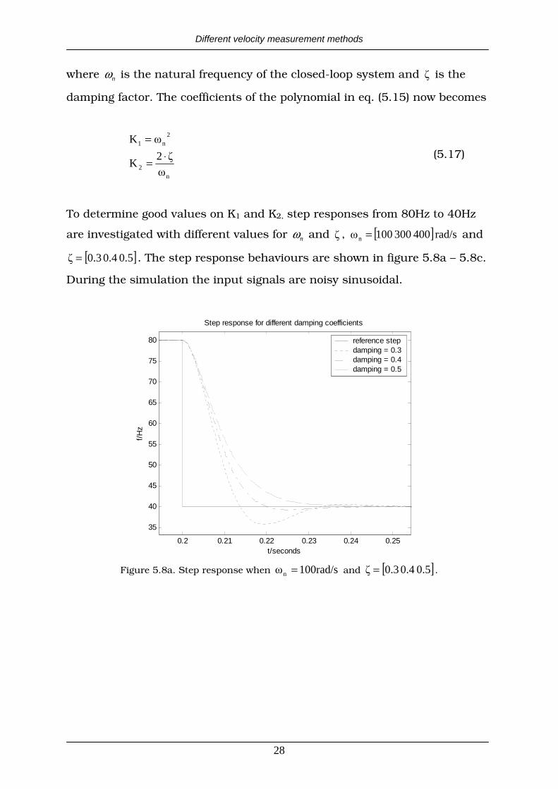
To determine good values on K1 and K2, step responses from 80Hz to 40Hz
are investigated with different values for nω and , [ ]rad/s400300100 n = and
[ ]0.5 0.4 0.3= . The step response behaviours are shown in figure 5.8a – 5.8c.
During the simulation the input signals are noisy sinusoidal.
0.2 0.21 0.22 0.23 0.24 0.25
35
40
45
50
55
60
65
70
75
80
t/seconds
f/H
z
Step response for different damping coefficients
reference stepdamping = 0.3damping = 0.4damping = 0.5
Figure 5.8a. Step response when 100rad/sn = and [ ]0.5 0.4 0.3= .

Different velocity measurement methods
29
0.2 0.205 0.21 0.215 0.22 0.225 0.23 0.235 0.24 0.245 0.25
35
40
45
50
55
60
65
70
75
80
t/seconds
f/Hz Step response for different damping coefficients
reference stepdamping = 0.3damping = 0.4damping = 0.5
Figure 5.8b. Step response when 300rad/sn = and [ ]0.5 0.4 0.3= .
0.2 0.205 0.21 0.215 0.22 0.225 0.23 0.235 0.24 0.245 0.25
35
40
45
50
55
60
65
70
75
80
t/seconds
f/HzStep response for different damping coefficients
reference stepdamping = 0.3damping = 0.4damping = 0.5
Figure 5.8c. Step response when 400rad/sn = and [ ]0.5 0.4 0.3= .
Different velocity measurement methods
30
As seen in figure 5.8a – 5.8c, different and nω give different over-shoot and
settling time. Some conclusions from these figures can be drawn:
• The damping factor determines the over-shoot and therefore also
affects the settling time of the step response, i.e. with small more
overshoot and oscillation is given.
• The natural frequency nω determines the settling-time of the step
response, i.e. with large nω faster step response is given. A limitation
of nω is, that if the signal is not clean (which of course it never is), with
large nω more variation around the estimated mean value is given.
In figure 5.8a – 5.8c it is seen that suitable values are 300rad/sn = and
0.4= , which mean fast settling time ( 12ms≈ ) and small oscillation ( 5%≥ )
are given. It is also seen that if nω is large (i.e. in this example rad/s400n = ),
the estimated speed fluctuates more around the correct value. This is
because the noise influences the system more, i.e. the gain in the control
loop becomes large ( 2n1K ∝ ).
If rad/s300n = , then an appropriate sampling time h has to be chosen. A
rule of thumb32 is 0.6h�0.1 n ≤⋅≤ . Also h has to be chosen to avoid aliasing.
In figure 5.9 the step response with 0.33msh = , 0.4= and rad/s300n = is
shown.
32Reference [15] p.130.

Different velocity measurement methods
31
0.2 0.205 0.21 0.215 0.22 0.225 0.23 0.235 0.24 0.245 0.25
40
45
50
55
60
65
70
75
80
f/Hz
t/seconds
Step response with chosen sample time
step referensestep response
Figure 5.9 Step response with rad/s300n = , 0.4= and 0.33msh = .
5.3. Tracking Demodulation- vs. Few Measurements methods
In figure 5.10 the step responses for Tracking Demodulation-, Few
Measurement Variance- and Few Measurements method are shown. The
Tracking Demodulation parameters are set to the most optimal, as in
chapter 5.2.1. The sensor signals are noisy sinusoidal.

Different velocity measurement methods
32
0.495 0.5 0.505 0.51 0.515 0.52 0.525 0.53
35
40
45
50
55
60
65
70
75
80
85
t/seconds
f/Hz Step response for different estimation methods
reference steptrackingFew Measurement Variance methodFew Measurement method
Figure 5.10. Step response for different estimation methods.
As seen in figure 5.10 the fastest and the most robust step response is
achieved with the Tracking Demodulation method. One of the reasons why
this method is faster is that it is independent of the estimated velocity. This
because a sampling frequency not much faster than 121 of the wheel speed
frequency33 is needed. Therefore the Few Measurements methods in the
simulation in figure 5.10 are unable to perform a new estimate every
millisecond, which is done by the Tracking Demodulation method.
Another advantage with the Tracking Demodulation method is that not so
much pre-filtering is needed. The Few measurements methods are rather
sensitive to noise compared to the Tracking Demodulation method. When
implementing the different methods, the calculation time differs a lot from
the different methods, especially the Few Measurements Variance method,
which has a lot of time demanding calculations. This means that the method
becomes slower.
33 In figure 5.10 the sensor frequency is 40Hz, which results in an appropriate sampling frequency of 1/(12*40) s � 2ms.
Different velocity measurement methods
33
5.4 Summary
Zero detection is an easy and fast method for determine the wheel speed
when driving at high velocities. As mentioned in chapter 4 this estimation is
too slow at low speed, and therefore two other methods are investigated.
These methods are Few Measurements- and Tracking Demodulation method.
The Few Measurements method is a fast method, which uses three
consecutive samples for determine the frequency of a single sinusoidal. This
method needs rather clean signals, and therefore pre-filtering is needed. An
improvement with this method is to make a fourth sample, and then
compute two frequency estimates, which use the statistical dependency of
these two estimates. Therefore more stable estimates are achieved.
The Tracking Demodulation method uses two sensors with a phase of 90
degrees between them. By making an estimation error between the correct-
and estimated position, it is possible to estimate the wheel speed.
Comparison of the Few Measurements- and Tracking Demodulation method
shows that the Tracking Demodulation method is faster and more robust at
low velocities, and is therefore suggested to be used. Another advantage is
that Tracking Demodulation method actually ”tracks” the correct position,
and could therefore be used to compensate for the wobble disturbance34 and
the fact that for different wheel speed, different amplitude in the sensor
signal is obtained.
34 See chapter 6.2.
Noise influence
34
6. Noise influence on- and filtering of the sensor signal and the frequency estimations
The output signal from the Solid-state sensors (which are used in the
rapport) is a pulse-train35. Therefore that signal is less sensitive to noise. In
this chapter, filtering of the Inductive Sensor signal from disturbances and
the digital filters used in the simulations and implementations are
discussed.
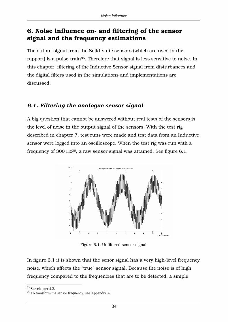
6.1. Filtering the analogue sensor signal
A big question that cannot be answered without real tests of the sensors is
the level of noise in the output signal of the sensors. With the test rig
described in chapter 7, test runs were made and test data from an Inductive
sensor were logged into an oscilloscope. When the test rig was run with a
frequency of 300 Hz36, a raw sensor signal was attained. See figure 6.1.
Figure 6.1. Unfiltered sensor signal.
In figure 6.1 it is shown that the senor signal has a very high-level frequency
noise, which affects the “true” sensor signal. Because the noise is of high
frequency compared to the frequencies that are to be detected, a simple
35 See chapter 4.2. 36 To transform the sensor frequency, see Appendix A.
Noise influence
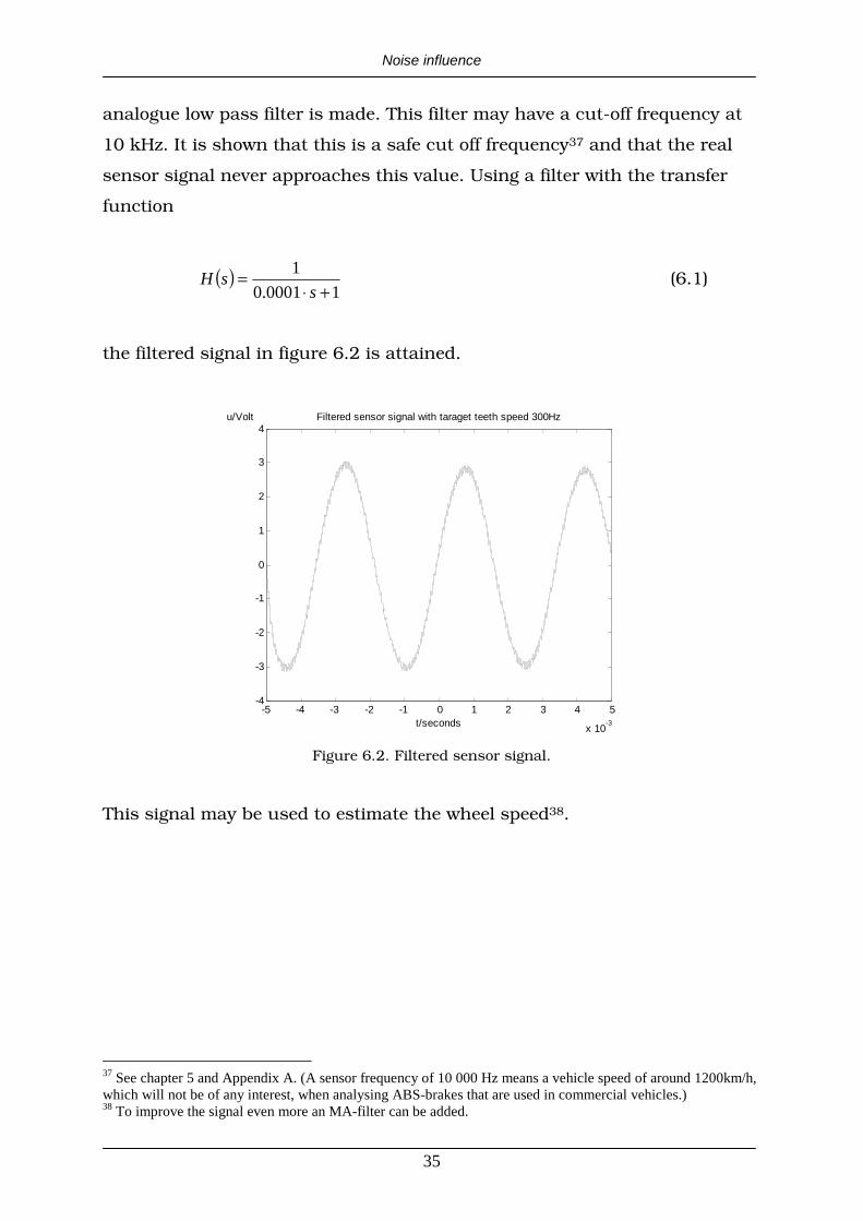
35
analogue low pass filter is made. This filter may have a cut-off frequency at
10 kHz. It is shown that this is a safe cut off frequency37 and that the real
sensor signal never approaches this value. Using a filter with the transfer
function
( )10001.0
1
+⋅=
ssH (6.1)
the filtered signal in figure 6.2 is attained.
-5 -4 -3 -2 -1 0 1 2 3 4 5
x 10-3
-4
-3
-2
-1
0
1
2
3
4
t/seconds
u/Volt Filtered sensor signal with taraget teeth speed 300Hz
Figure 6.2. Filtered sensor signal.
This signal may be used to estimate the wheel speed38.
37 See chapter 5 and Appendix A. (A sensor frequency of 10 000 Hz means a vehicle speed of around 1200km/h, which will not be of any interest, when analysing ABS-brakes that are used in commercial vehicles.) 38 To improve the signal even more an MA-filter can be added.

Noise influence
36
6.2. The Wobble disturbance
When a real target wheel in a test rig39 or in a vehicle is used, a disturbance
is received that varies due to the distance (air gap) between the sensor and
the target wheel. This is shown in the measured signal as changing
amplitude maximum and minimum, although travelling at the same velocity.
See figure 6.3. The disturbance (called a wobble disturbance) has come up
because of uneven distance between sensor and target wheel, which varies
periodically.
-0.2 -0.15 -0.1 -0.05 0 0.05 0.1 0.15 0.2-0.8
-0.6
-0.4
-0.2
0
0.2
0.4
0.6
t/seconds
u/VoltFiltered Sensor signal with wobble
Figure 6.3. Sensor signal with wobble.
Problems in the A/D-converter40 are due to this disturbance, i.e. maximum
resolution cannot always be obtained. Also when using the Tracking
Demodulation method (i.e. two sensors) on the test rig, i.e. different spacing
between the two sensors and the target wheel, which results in large
differences in the amplitude of the sensor signals are attained, due to the
distance between the sensors41. This results in violating the linearization in
eq. (5.12) of the closed loop system in eq. (5.13). To avoid the wobble
disturbance in the estimations, a peak-detection has to be made, i.e. how the
maximum/minimum values change over one turn of the wheel. Then a
compensation of the signal can be made through amplification.
39 See chapter 7. 40 See chapter 8. 41 See figure 7.2 in chapter 7.
Noise influence
37
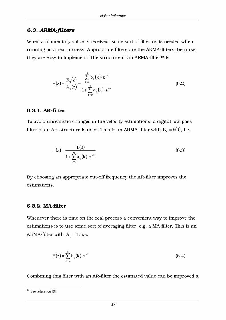
6.3. ARMA-filters
When a momentary value is received, some sort of filtering is needed when
running on a real process. Appropriate filters are the ARMA-filters, because
they are easy to implement. The structure of an ARMA-filter42 is
( ) ( )( )
( )
( )=
−
=
−
⋅+
⋅==
q
0k
kq
q
0k
kq
q
q
zka1
zkb
zA
zBzH (6.2)
6.3.1. AR-filter
To avoid unrealistic changes in the velocity estimations, a digital low-pass
filter of an AR-structure is used. This is an ARMA-filter with ( )0Bq b= , i.e.
( ) ( )( )
=
−⋅+=
q
0k
kq zka1
0bzH (6.3)
By choosing an appropriate cut-off frequency the AR-filter improves the
estimations.
6.3.2. MA-filter
Whenever there is time on the real process a convenient way to improve the
estimations is to use some sort of averaging filter, e.g. a MA-filter. This is an
ARMA-filter with 1Aq = , i.e.
( ) ( )=
−⋅=q
0k
kq zkbzH (6.4)
Combining this filter with an AR-filter the estimated value can be improved a
42 See reference [9].
Noise influence
38
lot. The MA-filter can be used when reducing the noise from the sensor
signal, but also to achieve better speed estimation.
6.4 Summary
When real tests and implementations of the different wheel speed
estimations have been performed on the real test rig, filtering is needed. The
inductive sensor signal has a high frequency component added to the ”true”
frequency, and therefore an analogue low pass filter is added as a pre-
filtering. The wobble disturbance could give problems, and has to be taken
under consideration. When ether there is time in an implementational
aspect, the ARMA-filters are one way to stabilize, both in the A/D-
conversion, and when an estimated velocity is obtained.
Real sensor testing
39
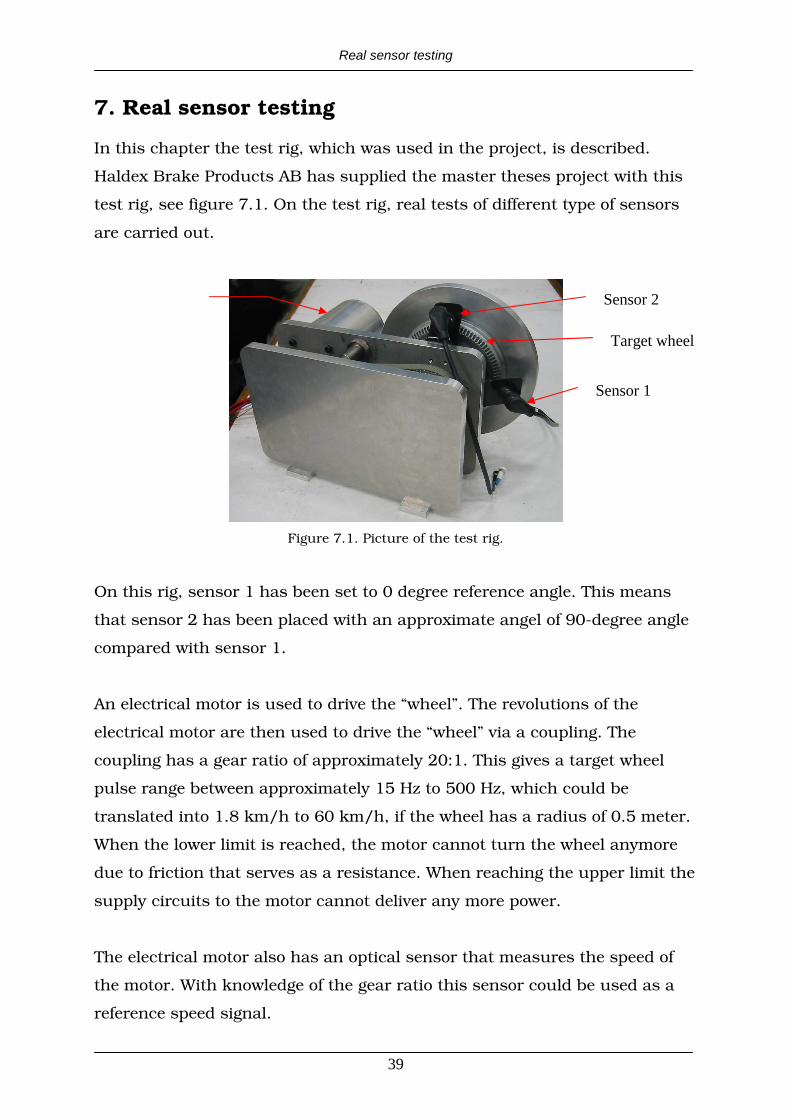
7. Real sensor testing
In this chapter the test rig, which was used in the project, is described.
Haldex Brake Products AB has supplied the master theses project with this
test rig, see figure 7.1. On the test rig, real tests of different type of sensors
are carried out.
Figure 7.1. Picture of the test rig.
On this rig, sensor 1 has been set to 0 degree reference angle. This means
that sensor 2 has been placed with an approximate angel of 90-degree angle
compared with sensor 1.
An electrical motor is used to drive the “wheel”. The revolutions of the
electrical motor are then used to drive the “wheel” via a coupling. The
coupling has a gear ratio of approximately 20:1. This gives a target wheel
pulse range between approximately 15 Hz to 500 Hz, which could be
translated into 1.8 km/h to 60 km/h, if the wheel has a radius of 0.5 meter.
When the lower limit is reached, the motor cannot turn the wheel anymore
due to friction that serves as a resistance. When reaching the upper limit the
supply circuits to the motor cannot deliver any more power.
The electrical motor also has an optical sensor that measures the speed of
the motor. With knowledge of the gear ratio this sensor could be used as a
reference speed signal.
Sensor 1
Sensor 2
Target wheel

Real sensor testing
40
As seen in figure 7.2 the sensors could be placed with different lengths from
the target wheel.
Figure 7.2. Picture of the sensor position towards the target wheel.
In all the tests carried out, the sensors have been placed as close as
possible, i.e. the sensors should not touch the target wheel.
Optical sensor
Implementation
41
8. Implementation methods into a microcontroller
In this chapter the implementation of zero detection and few measurements
method into a microcontroller are discussed. General description of the
microcontroller, and different aspects of what is needed to be considered
when the methods are implemented, is brought up.
8.1. The microcontroller
A motor control development card has been put to our disposal. This card is
equipped with a microcontroller. This processor can be run at clock
frequencies up to 40 MHz. It contains several useful things that can be used
in an application like this, e.g. digital signal processor, 10 and 12-bit A/D-
converter. It also contains CAN (Controller Area Network), SPI (Serial
Peripheral Interface), UART (Universal Asynchronous Receiver-Transmitter)
and I2C (Integrated Circuit) interface. These interfaces can be used to
communicate with other processors or devices that need information about
the result of the velocity calculation. The circuit also has five timers and
several ports that can be used as interrupts. After each interrupt a certain
code can be executed.
The processor is easily programmed with the aid of MPLAB (Microchips
programming interface), which also contains software simulator. This
software simulator can be used to verify the functionality of the project
before downloading it into the circuit.
8.2. Pre-signal processing for Inductive sensors
A restriction that can arise when using the A/D-converter in the micro
controller is that it is only possible to A/D-convert voltage levels between
Vdd and Vcc supplied to the circuit, in this case 0 and 5V. This means that
with an inductive sensor, only half of the period would be A/D-converted
correctly. The negative part would be A/D-converted to zero. A
Implementation
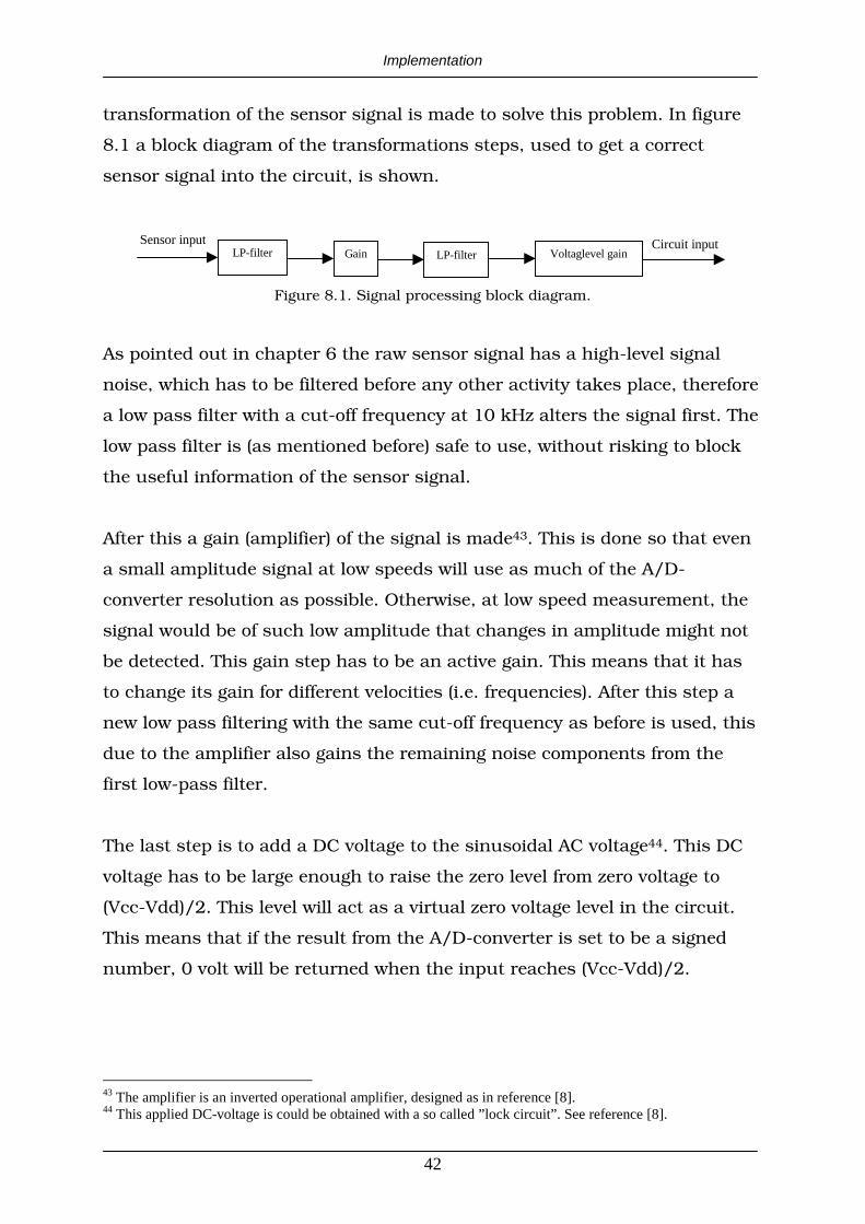
42
transformation of the sensor signal is made to solve this problem. In figure
8.1 a block diagram of the transformations steps, used to get a correct
sensor signal into the circuit, is shown.
LP-filter Gain LP-filter Voltaglevel gainSensor input Circuit input
Figure 8.1. Signal processing block diagram.
As pointed out in chapter 6 the raw sensor signal has a high-level signal
noise, which has to be filtered before any other activity takes place, therefore
a low pass filter with a cut-off frequency at 10 kHz alters the signal first. The
low pass filter is (as mentioned before) safe to use, without risking to block
the useful information of the sensor signal.
After this a gain (amplifier) of the signal is made43. This is done so that even
a small amplitude signal at low speeds will use as much of the A/D-
converter resolution as possible. Otherwise, at low speed measurement, the
signal would be of such low amplitude that changes in amplitude might not
be detected. This gain step has to be an active gain. This means that it has
to change its gain for different velocities (i.e. frequencies). After this step a
new low pass filtering with the same cut-off frequency as before is used, this
due to the amplifier also gains the remaining noise components from the
first low-pass filter.
The last step is to add a DC voltage to the sinusoidal AC voltage44. This DC
voltage has to be large enough to raise the zero level from zero voltage to
(Vcc-Vdd)/2. This level will act as a virtual zero voltage level in the circuit.
This means that if the result from the A/D-converter is set to be a signed
number, 0 volt will be returned when the input reaches (Vcc-Vdd)/2.
43 The amplifier is an inverted operational amplifier, designed as in reference [8]. 44 This applied DC-voltage is could be obtained with a so called ”lock circuit”. See reference [8].
Implementation
43
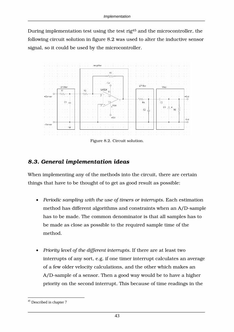
During implementation test using the test rig45 and the microcontroller, the
following circuit solution in figure 8.2 was used to alter the inductive sensor
signal, so it could be used by the microcontroller.
Figure 8.2. Circuit solution.
8.3. General implementation ideas
When implementing any of the methods into the circuit, there are certain
things that have to be thought of to get as good result as possible:
• Periodic sampling with the use of timers or interrupts. Each estimation
method has different algorithms and constraints when an A/D-sample
has to be made. The common denominator is that all samples has to
be made as close as possible to the required sample time of the
method.
• Priority level of the different interrupts. If there are at least two
interrupts of any sort, e.g. if one timer interrupt calculates an average
of a few older velocity calculations, and the other which makes an
A/D-sample of a sensor. Then a good way would be to have a higher
priority on the second interrupt. This because of time readings in the
45 Described in chapter 7

Implementation
44
A/D-conversion interrupt, which would be affected by interrupts,
resulting in a greater time value than it should have.
• Calculation optimisation. Depending on the circuit used, and
programming language used, a calculation can take different amount
of time. E.g. in the math library that is used in C, a multiplication or a
division could take quite a long time. This is because methods are
implemented with the use of recursive or iterative numerical
functions. In this circuit using the DSP-functions could solve this
problem, and make the calculations somewhat less time-consuming.
In the following pages, the structures, which were used to implement velocity
measurement using Hall-Effect sensor, and also analogue inductive sensor
with the method of Few Measurements methods, are shown.
8.4. Implementation of Few Measurements method
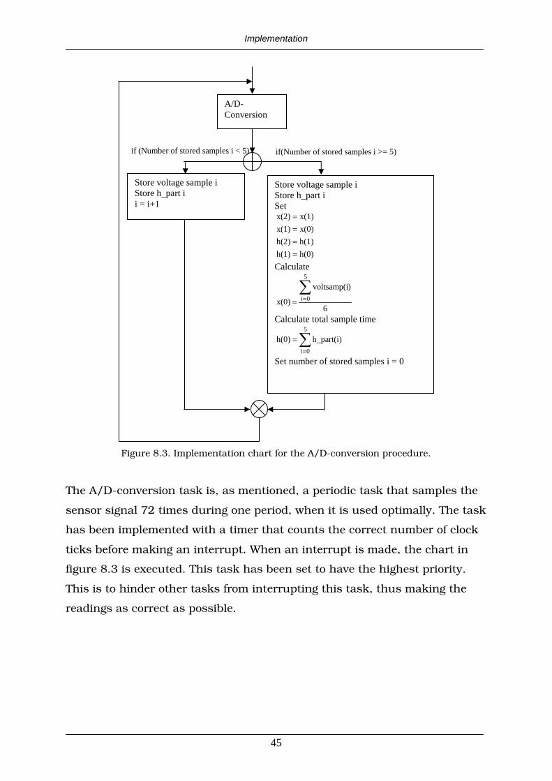
In figure 8.3 – 8.4, the charts of how Few Measurements method was
implemented into the microcontroller to measure velocity with an inductive
sensor, is shown. This implementation contains two tasks; a main task that
executes all the time, and one periodic task, which executes so often that 12
samples per sinusoidal period is achieved. Each sample is an average of 6
samples, which means that a sample period of 72 times the sinusoidal
frequency should be used to achieve the best result.
Implementation
45
Figure 8.3. Implementation chart for the A/D-conversion procedure.
The A/D-conversion task is, as mentioned, a periodic task that samples the
sensor signal 72 times during one period, when it is used optimally. The task
has been implemented with a timer that counts the correct number of clock
ticks before making an interrupt. When an interrupt is made, the chart in
figure 8.3 is executed. This task has been set to have the highest priority.
This is to hinder other tasks from interrupting this task, thus making the
readings as correct as possible.
A/D-Conversion
if (Number of stored samples i < 5) if(Number of stored samples i >= 5)
Store voltage sample i Store h_part i i = i+1
Store voltage sample i Store h_part i Set
h(0)h(1)
h(1)h(2)
x(0)x(1)
x(1)x(2)
====
Calculate
6
)voltsamp(i
x(0)
5
0i==
Calculate total sample time
=
=5
0i
h_part(i)h(0)
Set number of stored samples i = 0
Implementation
46
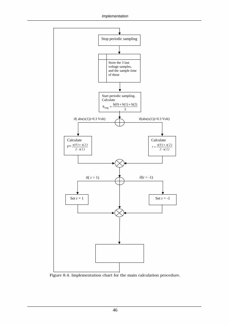
Figure 8.4. Implementation chart for the main calculation procedure.
Stop periodic sampling
Store the 3 last voltage samples, and the sample time of these
Start periodic sampling. Calculate
3
h(2)h(1)h(0)havg
++=
Calculate
r=)1(x2
)2(x)0(x
⋅+
Calculate
)2(x2
)2(x)0(xr
⋅+=
if( abs(x(1))>0.3 Volt) if(abs(x(1))<0.3 Volt)
Set r = 1 Set r = -1
if( r > 1) if(r < -1)
Implementation
47
The task in figure 8.4 is placed in main, which means that it is executing
whenever the sampling task is not. One stoppage is made on the A/D-
conversion task. This is done when the calculation loop reads new values to
base its calculations on. If a stoppage is not made, this could mean that the
A/D-conversion loop could break, and modify the variables that the main
task is about to read, resulting in a calculation result that might be wrong.
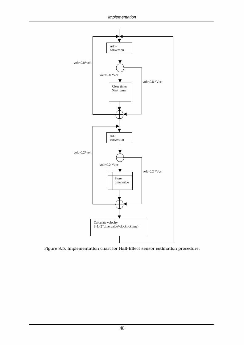
8.5. Implementation of Hall-Effect sensor measurement
In figure 8.5 the chart of how Hall-Effect sensor signals can be measured by
the microcontroller is shown. The loop in this figure is the main task and will
execute all the time. Of course this does not take any of the above-mentioned
points about sample time and priority under consideration. The choice of
allowing this task to execute all the time is, because of the nature of the
digitised signal that a Hall-Effect sensor delivers. It changes (as mentioned)
from 0 volt to e.g. 5 volt, at the point when a sinusoidal period changes from
negative to positive value (zero crossing). The opposite happens at a positive
to negative value change. This loop then allows the processor to catch a
change as close as possible.
If the sampling would instead have been put into a periodic sampling, then
there could be a jitter in the time measurement, which would then turn up
in the calculated velocity calculation as a variation in velocity that would be
larger than it should be.
Implementation
48
Calculate velocity f=1/(2*timervalue*clockticktime)
A/D-convertion
Store timervalue
volt<0.2 *Vcc
volt>0.2 *Vcc
volt>0.2*volt
A/D-convertion
volt>0.8 *Vcc
volt<0.8 *Vcc
volt<0.8*volt
Clear timerStart timer
Figure 8.5. Implementation chart for Hall-Effect sensor estimation procedure.
Implementation
49
8.6 Summary
When the estimation methods are implemented there are some common
factors that have to be considered. First, it is necessary to use periodic
sampling, which is carried out with the help of timers or interrupts46 in a
microcontroller, because of the importance to obtain samples as often as the
required sample time. Second, the time demanding calculations in the
estimation methods, e.g. multiplications and divisions, have to be optimized
to minimize the calculation time.
46 If there are more than one interrupt, it is suggested to have different priority of these interrupts.
Conclusions
50
9. Conclusions
As discussed in the rapport, problems arise when trying to achieve correct
velocity estimation below 20 km/h. When using an inductive sensor, the first
problem that occurs is that the amplitude level of the signal is too low. This
means that the signal is very sensitive to noise and may give faulty velocity
estimations when zero detection algorithms are used. A faulty zero might be
detected.
It is proposed to use a first order filter to get rid of the noise, and an active
amplifier will amplify the signal with different gain, determined by the
current frequency of the target wheel, and current distance between sensor
and target wheel. A Hall Effect sensor can be used to get around this
problem. This sensor gives a good, stable signal that changes between low
and high state, as the teeth of the target wheel pass by. But also, this sensor
has problems below 20 km/h. In this case, the problem is that the time
between states changes at these speeds start to rise to such values that it
will be impossible to calculate velocity estimation within demanded
deadlines.
By using either Few Measurement Estimation with or without variance
compensation or Tracking Demodulation, which both have been presented in
the rapport, faster wheel speed estimations are achieved. These methods use
the inductive sensor. It will be possible to calculate new frequency
estimations at least every 121 of a period. This will then give possibilities to
achieve valid frequency estimations below 20 km/h. These methods will also
give a better estimate, because several estimations can be made within
deadline and an average of these estimations can be calculated.
Comparisons between these two methods have been made. These show that
better estimations are achieved with the Tracking Demodulation than the
Few Measurements methods. Another advantage of Tracking Demodulation
is that it has less time consuming calculations than the Few Measurements.
Conclusions
51
A disadvantage of the Tracking Demodulation method is that two inductive
sensors have to be used, and these two have to be placed in a 90 degree
angle.
As a conclusion from these comparisons, a suggestion is that velocity
measurement shall be made by scheduling the use of the methods. At
velocities above 20 km/h, zero detection could be used. Then, if two
inductive sensors are used, these can be used to achieve an average value
between these two sensors. Below 20 km/h it is suggested that Tracking
Demodulation shall be used, instead of Few Measurement. Mainly because it
is less time consuming when calculations are made, and it is independent of
the wheel speed which the other methods are not.
Finally we would like to thank Haldex Brake Products which gave us the
opportunity to do this master thesis project. We would especially like to
thank Ola Nockhammar, the supervisor of this project, for his insightful
thoughts and ideas which encouraged and inspired us. Thanks also to
Anders Rantzer, our supervisor at the Department of Automatic Control,
Lund Institute of Technology.
Appendix
52
Appendix A
A.1. Wheel velocity
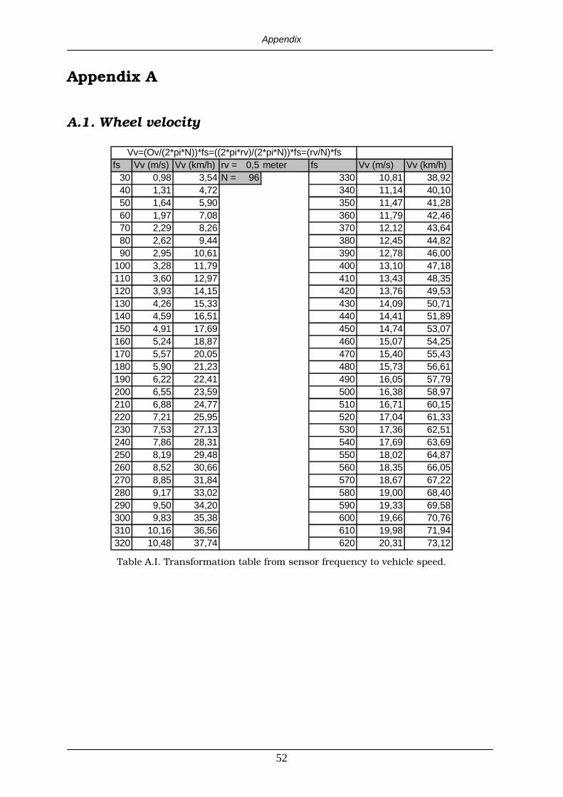
fs Vv (m/s) Vv (km/h) rv = 0,5 meter fs Vv (m/s) Vv (km/h)30 0,98 3,54 N = 96 330 10,81 38,9240 1,31 4,72 340 11,14 40,1050 1,64 5,90 350 11,47 41,2860 1,97 7,08 360 11,79 42,4670 2,29 8,26 370 12,12 43,6480 2,62 9,44 380 12,45 44,8290 2,95 10,61 390 12,78 46,00
100 3,28 11,79 400 13,10 47,18110 3,60 12,97 410 13,43 48,35120 3,93 14,15 420 13,76 49,53130 4,26 15,33 430 14,09 50,71140 4,59 16,51 440 14,41 51,89150 4,91 17,69 450 14,74 53,07160 5,24 18,87 460 15,07 54,25170 5,57 20,05 470 15,40 55,43180 5,90 21,23 480 15,73 56,61190 6,22 22,41 490 16,05 57,79200 6,55 23,59 500 16,38 58,97210 6,88 24,77 510 16,71 60,15220 7,21 25,95 520 17,04 61,33230 7,53 27,13 530 17,36 62,51240 7,86 28,31 540 17,69 63,69250 8,19 29,48 550 18,02 64,87260 8,52 30,66 560 18,35 66,05270 8,85 31,84 570 18,67 67,22280 9,17 33,02 580 19,00 68,40290 9,50 34,20 590 19,33 69,58300 9,83 35,38 600 19,66 70,76310 10,16 36,56 610 19,98 71,94320 10,48 37,74 620 20,31 73,12
Vv=(Ov/(2*pi*N))*fs=((2*pi*rv)/(2*pi*N))*fs=(rv/N)*fs
Table A.I. Transformation table from sensor frequency to vehicle speed.

Appendix
53
Appendix B
B.1. Proof of Few Measurement method
With a signal as )tcos(Ax(t) +⋅⋅= it is possible to derive an estimate as
T
arccos(r)T)cos(r =⋅= .
This can be done if the three consecutive samples are
[ ][ ][ ] )T2cos(A2x
)Tcos(A1x
)cos(A0x
θ+⋅⋅ω⋅=θ+⋅ω⋅=
θ⋅=
which results in
[ ] [ ][ ] θ+⋅ω⋅⋅
θ+⋅⋅ω+θ⋅=θ+⋅ω⋅⋅
θ+⋅⋅ω⋅+θ⋅=⋅+=
))Tcos(2(A
))T2cos()(cos(A
)Tcos(A2
)T2cos(A)cos(A
1x2
2x0xr
=−ω⋅⋅=ω⋅⋅
ω⋅⋅ω⋅⋅=ω⋅⋅=
θ⋅⋅ω⋅−θ⋅⋅ω⋅θ⋅ω⋅⋅−θ⋅ω⋅+θ=
1)T(cos2)T2cos(
)Tcos()Tsin(2)T2sin(
)sin()Tsin(2)cos()Tcos(2
)sin()T2sin()cos()T2cos()cos(2
=θ⋅ω⋅⋅−θ⋅ω⋅⋅
θ⋅ω⋅⋅ω⋅⋅−θ−θ⋅ω⋅⋅+θ=)sin()Tsin(2)cos()Tcos(2
)sin()Tcos()Tsin(2)cos()cos()T(cos2)cos( 2
)Tcos())sin()Tsin()cos()T(cos(2
))sin()Tsin()cos()T(cos()Tcos(2 ω⋅=θ⋅ω⋅−θ⋅ω⋅⋅
θ⋅ω⋅−θ⋅ω⋅⋅ω⋅⋅= FINISHED
References
54
References
[1]. Adelson Ronald M., Frequency Estimation from Few Measurements, 1997, Academic Press, Journal: Digital Signal Processing
[2]. AI-Tek Instruments Inc., Sensors, http://www.aitekinstruments.com/pdf/sensors.pdf , 2003-07-07
[3]. Cheng David K., Field and Wave Electromagnetics, Second Edition, 1992, Addison Wesley Publishing Company Inc, ISBN 0-201-12819-5
[4]. Dietmayer Klaus ,Schmei�er Fritz, Rotational Speed Sensors KMI15/16, 1999, Philips
Electronics N.V., http://www.semiconductors.philips.com/acrobat/applicationnotes/KMI16-15.pdf , 2003-10-28
[5]. Honeywell, Hall Effect Sensing and Application, MICRO SWITCH Sensing and Control, http://content.honeywell.com/sensing/prodinfo/solidstate/technical/hallbook.pdf , 2003-10-28
[6]. Lequesne B. , Pawlak A. , Schroeder T., Magnetic velocity sensors, 1991, IEEE, Journal: Industry Applications Society Annual Meeting, 1991., Conference Record of the 1991 IEEE
[7]. Limpert Rudolf, Brake Design and Safety, Second Edition, 1999, Society of Automotive Engineers, Inc., ISBN 1-56091-915-9
[8]. Lundqvist Hans, Analog kretselektronik, 1992, Liber Utbildning, ISBN 91-634-1551-8
[9]. Monson Hayes, Statistical digital signal processing and modeling, 1996, John Wiley, ISBN 0-47-159431-8
[10]. Morgan Don, Tracking Demodulation, 2001-02-26, www.embedded.com, http://www.embedded.com/story/OEG20010221S0089 , 2003-10-28
[11]. Proakis John G., Manolakis Dimitris G., Digital Signal Processing, Principles, Algorithms, and
applications Third edition, 1996, Prentice-Hall Inc., ISBN 0-13-394289-9
[12]. Robert Bosch GmbH, Brake Systems for passenger cars, second edition, 1995, Robert Bosch GmbH
[13]. Slotine E. Jean-Jacques,Weiping Li, Applied Nonlinear Control, 1991, Prentice-Hall Inc., ISBN 0-13-040890-5
[14]. Wong J.Y. , Theory of ground vehicles, 2001, John Wiley & Sons Inc. , ISBN 0-471-35461-9
[15]. Åström Karl J. Björn Wittenmark, Computer-Controlled Systems Theory and Design, Third
Edition, 1997, Prentice-Hall Inc., ISBN 0-13-314899-8