Improving Variable D D - repositorio-aberto.up.pt · conjuntos de dados de cancro da mama em...
185
Improving Variable Selection and Mammography-based Machine Learning Classifiers for Breast Cancer CADx Noel Pérez Pérez Thesis submitted to the Faculty of Sciences of the University of Porto, University of Aveiro and University of Minho in partial fulfillment of the requirements for the degree of Doctor of Philosophy in Computer Science March 2015 Improving Variable Selection and Mammography-based Machine Learning Classifiers for Breast Cancer CADx Noel Pérez Pérez PhD FCUP UA UM 2015 3.º CICLO D D
Transcript of Improving Variable D D - repositorio-aberto.up.pt · conjuntos de dados de cancro da mama em...

Improving Variable Selection and Mammography-based Machine Learning Classifiers for Breast Cancer CADx
Noel Pérez Pérez
Thesis submitted to the Faculty of Sciences of the University of Porto, University of Aveiro and University of Minho in partial fulfillment of the requirements for the degree of Doctor of Philosophy in Computer Science
March 2015
Improving Variable Selection and M
amm
ography-based M
achine Learning Classifiers for Breast C
ancer CAD
xN
oel Pérez PérezP
hD
FCUPUAUM
2015
3.ºCICLO
DD

DImproving Variable Selection and Mammography-based Machine Learning Classifiers for Breast Cancer CADxNoel Pérez PérezDoctoral Program in Computer Science of the Universities of Minho, Aveiro and PortoDepartment of Computer ScienceMarch 2015
SupervisorMiguel Angel Guevara López, Senior Researcher, Institute of Electronics and Telematics Engineering of Aveiro, University of Aveiro
Co-Supervisor Augusto Marques Ferreira da Silva, Assistant Professor, Department of Electronics, Telecommunications and Informatics, University of Aveiro

To My Parents Magalys and Noel Pérez

Acknowledgement
Many people have played important roles during the course of my doctoral studies. It is time
to reflect on those whose support and encouragement were essential components for a
successful completion of this thesis.
I am grateful to my supervisor Prof. Miguel Angel Guevara López for introducing me to the
field of medical image analysis and for his supervision during this thesis.
Special thanks to Prof. Augusto Silva, my co-supervisor (IEETA) for his helpful remarks
during our scientific discussion.
I am also fortunate for the time I spent at the Laboratory of Optics and Experimental
Mechanics (LOME) - Institute of Mechanical Engineering and Industrial Management
(INEGI), University of Porto. All the members deserve special recognition for the friendly
atmosphere, supportive environment, and logistic assistance they provided.
I also wish to acknowledge the FCT (Fundação para a Ciência e a Tecnologia) for the
financial support (grant SFRH/BD/48896/2008).
I am also grateful to Prof. Fernando Silva, Alexandra Ferreira (DCC) and Sofia Santos
(FCUP) for their valuable help and guidance during this time.
I am greatly indebted to Dr. Alexis Oliva and his family for their help, support and fraternal
love during this hardest time.
Thanks to my friends in Portugal and Cuba for their friendship and support. All their
comments were always well received.
Finally, I would like to show my deepest appreciation to my parents; Magalys and Noel, my
sisters and nieces, my brother in law Danilo, and my girlfriend Lizbeth Oliva for their
unparalleled love and support.

i
Abstract
Breast Cancer is a major concern and the second-most common and leading cause of cancer
deaths among women. According to public statistics in Portugal estimates point to 4500 new
diagnosed cases of breast cancer and 1600 women death from this disease. At present, there
are no effective ways to prevent breast cancer, because its cause remains unknown. However,
efficient diagnosis of breast cancer in its early stages can give a woman a better chance of full
recovery. Breast imaging, which is fundamental to cancer risk assessment, detection,
diagnosis and treatment, is undergoing a paradigm shift: the tendency is to move from a
primarily qualitative interpretation to a more quantitative-based interpretation model. In term
of diagnosis, the mammography and the double reading of mammograms are two useful and
suggested techniques for reducing the proportion of missed cancers. But the workload and
cost associated are high.
Breast Cancer CADx systems is a more recent technique, which has improved the AUC-based
performance of radiologists and the classification of breast cancer in its early stages. But the
performance of current commercial CADx systems still needs to be improved so that they can
meet the requirements of clinics and screening centers.
Feature selection techniques constitute one of the most important steps in the lifecycle of
Breast Cancer CADx systems. It presents many potential benefits such as: facilitating data
visualization and data understanding, reducing the measurement and storage requirements,
reducing training and utilization times and, defining the curse of dimensionality to improve
the predictions performance. It is therefore convenient that feature selection methods are fast,
scalable, accurate and possibly with low algorithmic complexity.
This thesis was motivated by the need of developing new feature selection methods to provide
more accurate and compact subsets of features to feed machine learning classifiers supporting
breast cancer diagnosis. In our study, we realized that most of the developed approaches were
focused on the wrapper or hybrid paradigm and, in fewer degrees on filter paradigm. We
considered exploring the filter paradigm because filter methods provide lower algorithmic

ii
complexity, faster performance and are independent of classifiers. However, feature selection
methods based on this paradigm present two main limitations: (1) ignore the dependencies
among features and (2) assume a given distribution (Gaussian in most cases) from which the
samples (observations) have been collected. In addition, assuming a Gaussian distribution
includes the difficulties to validate distributional assumptions because of small sample sizes.
The first contribution of this thesis is an ensemble feature selection method (named RMean)
based on the mean criteria (assigned by the mean of the feature) for indexing relevant
features. When applied to the breast cancer datasets under study, the subsets of ranked
features produced by using the RMean method improved the AUC performance in almost all
the explored machine learning classifiers. Despite the good performance of the RMean
method, it still preserves the limitations of filter methods and this may lead the Breast Cancer
CADx methods to classification performances bellow of its potential.
To overcome these limitations, the second contribution proposes a new feature selection
method (named uFilter) based on the Mann Whitney U-test for ranking relevant features,
which asses the relevance of features by computing the separability between class-data
distribution of each feature. The uFilter method solves some difficulties remaining on
previous developed methods, such as: it is effective in ranking relevant features independently
of the samples sizes (tolerant to unbalanced training data); it does not need any type of data
normalization; and the most important, it presents a low risk of data overfitting. When applied
to the breast cancer datasets under study, the uFilter method statistically outperformed the U-
Test (baseline method), RMean (contribution 1) and four classical feature selection methods.
This method revealed competitive and appealing cost-effectiveness results on selecting
relevant features, as a support tool for breast cancer CADx methods. Finally, the redundancy
analysis as a complementary step to the uFilter method provided us an effective way for
finding optimal subsets of features.

iii
Resumo
O Cancro da Mama é segunda causa de morte mais comum entre as mulheres, sendo a mais
comum dentro das mortes por cancro. De acordo com as estatísticas nacionais, estima-se que
em Portugal sejam diagnosticados 4500 novos casos por ano que acabam por vitimar 1600
mulheres. Atualmente não há formas eficazes de prevenir o cancro da mama uma vez que a
sua causa permanece desconhecida. Contudo, o diagnóstico precoce do cancro da mama
aumenta a possibilidade de uma recuperação completa. A imagiologia da mama, que é
fundamental para a avaliação de risco, detecção, diagnóstico e terapia está sob um processo de
mudança de paradigma: a tendência é passar de uma interpretação maioritariamente
qualitativa para modelos de interpretação mais quantitativos. Em termos de diagnóstico, a
mamografia e a avaliação dos mamogramas por dois profissionais são técnicas úteis que são
sugeridas para a redução da proporção de cancros não diagnosticados. No entanto, a carga de
trabalho e os custos envolvidos são elevados.
Os sistemas de Diagnóstico Assistido por Computador (CADx) são uma técnica recente que
tem melhorado o desempenho dos radiologistas e a classificação dos casos de cancro em
estágios iniciais. Contudo, o desempenho dos sistemas comerciais de CADx necessita de ser
melhorado para que cumpram os requisitos estabelecidos para a sua utilização na prática
clínica.
As técnicas de seleção de caraterísticas são um dos passos mais importantes no ciclo de vida
de um sistema de CADx. Estas técnicas apresentam vários benefícios potenciais, tais como:
facilitam a visualização e compreensão dos dados, reduzem os requisitos de medição e
armazenamento, reduzem os tempo de treino e de resposta dos sistemas, evitando os
problemas da alta dimensionalidade e permitindo aumentar o poder preditivo dos sistemas.
Por isso, é desejável que os métodos de seleção de caraterísticas sejam rápidos, escaláveis,
exatos e com baixa complexidade algorítmica.
Esta tese foi motivada pela necessidade de novos métodos de seleção de caraterísticas que
permitam obter subconjuntos de caraterísticas mais compactos e discriminativos para o treino
de classificadores de suporte ao diagnostico do cancro da mama. Neste estudo, constatou-se
que a maior parte das abordagens focam-se nos paradigmas wrapper, híbrido e em menor grau

iv
no paradigma filtro. Esta tese assenta na exploração do paradigma filtro porque envolve uma
complexidade algorítmica mais baixa, desempenho mais rápido e porque é independente de
classificadores. No entanto, os métodos de seleção de caraterísticas baseados neste paradigma
tem duas limitações principais: (1) ignoram dependências entre caraterísticas e (2) assumem
uma dada distribuição (Gaussiana na maior parte dos casos) a partir da qual as amostras
(observações) são recolhidas. A assunção de distribuição Gaussiana pode trazer problemas
adicionais relacionados com dificuldades em validar as assunções desta distribuição,
principalmente quando o número de amostras é baixo.
A primeira contribuição desta tese é um método ensemble de seleção de caraterísticas
(denominado RMean) baseado no critério da média (atribuida pelo promedio da característica)
para indexação de caraterísticas relevantes. Quando aplicado a conjuntos de dados de cancro
da mama, o RMean permite aumentar o desempenho ao nível do AUC (área debaixo da curva
da caraterística de operação do receptor) em quase todos os algoritmos de classificação
explorados. Apesar da boa performance do método RMean, este método sofre das limitações
dos métodos de filtro o que pode levar a desempenhos do sistema CADx abaixo do seu
potencial.
Tendo em vista ultrapassar estas limitações, a segunda contribuição propõe um novo método
de seleção de caraterísticas (denominado uFitler) baseado no teste U de Mann Whitney para
ordenar as características por relevância. A avaliação da relevância é feita através do cálculo
da separabilidade entre as distribuições de cada classe para cada caraterística. O método
uFilter resolve alguns dos problemas dos métodos anteriores, tais como: é eficaz a ordenar as
caraterísticas por relevância independentemente do tamanho da amostra (sendo tolerante a
desequilíbrios nos dados de treino); não necessita de normalização dos dados; e, o mais
importante, apresenta um risco baixo de sobreajuste aos dados. Quando aplicado aos
conjuntos de dados de cancro da mama em estudo, o uFilter obteve melhores resultados com
significado estatístico que o teste de U, RMean (contribuição 1) e que quatro métodos
clássicos de seleção de caraterísticas. Este método mostrou-se competitivo e apelativo em
termos de custo-eficiência na seleção de caraterísticas relevantes para sistemas de CADx de
Cancro da Mama. Finalmente, um passo complementar, a análise de redundância mostrou ser
uma forma eficaz de encontrar subconjuntos ótimos de caraterísticas.

v
Contents
List of Figures .................................................................................................................... viii
List of Tables ........................................................................................................................ xi
Acronyms ........................................................................................................................... xiii
Chapter 1: Introduction ....................................................................................................... 1
1.1. Background ..............................................................................................................2
1.1.1. Breast Cancer ....................................................................................................2
1.1.2. BI-RADS ..........................................................................................................3
1.1.3. Mammography ..................................................................................................5
1.1.4. Masses ..............................................................................................................6
1.1.5. Microcalcifications ............................................................................................8
1.1.6. Early Detection .................................................................................................9
1.1.7. Breast Cancer CAD ......................................................................................... 10
1.1.8. Features Selection Methods ............................................................................. 12
1.1.9. Machine Learning Classifiers .......................................................................... 13
1.2. Motivation and Objectives ...................................................................................... 13
1.3. Thesis Statement .................................................................................................... 15
1.4. Summary of Contributions...................................................................................... 16
1.5. Thesis Outline ........................................................................................................ 16
1.6. Auto-Bibliography.................................................................................................. 18
Chapter 2: State of the Art ................................................................................................. 20
2.1. Breast Cancer Supporting Repositories ................................................................... 21
2.2. Clinical and Image-based Descriptors for Breast Cancer ......................................... 24
2.2.1. Clinical Descriptors ......................................................................................... 24
2.2.2. Image-based Descriptors ................................................................................. 25
2.3. Feature Selection Methods...................................................................................... 36
2.3.1. Filter Paradigm ................................................................................................ 38
vi
2.3.2. Wrapper Paradigm........................................................................................... 39
2.3.3. Hybrid Paradigm ............................................................................................. 40
2.3.4. Related Works ................................................................................................. 41
2.3.5. Comparative Analysis ..................................................................................... 44
2.4. Machine Learning Classifiers ................................................................................. 46
2.4.1. k-Nearest Neighbors ........................................................................................ 47
2.4.2. Artificial Neural Networks .............................................................................. 48
2.4.3. Support Vector Machines ................................................................................ 49
2.4.4. Linear Discriminant Analysis .......................................................................... 50
2.4.5. Related Works ................................................................................................. 51
2.5. CADe and CADx systems in Breast Cancer ............................................................ 55
2.6. Conclusions ............................................................................................................ 60
Chapter 3: Experimental Methodologies ........................................................................... 62
3.1. Datasets .................................................................................................................. 63
3.1.1. BCDR ............................................................................................................. 63
3.1.2. DDSM ............................................................................................................. 65
3.1.3. Considered Clinical and Image-based Descriptors ........................................... 67
3.2. Feature Selection .................................................................................................... 73
3.3. Exploring Classifiers .............................................................................................. 74
3.4. The RMean Method ................................................................................................ 77
3.5. Experimental Setup ................................................................................................ 78
3.6. Results and Discussions .......................................................................................... 80
3.6.1. First Experiment .............................................................................................. 80
3.6.2. Second Experiment ......................................................................................... 96
3.6.3. Global Discussion of Experiments ................................................................. 102
3.7. Conclusions .......................................................................................................... 107
Chapter 4: The uFilter Method ........................................................................................ 108
4.1. Introduction .......................................................................................................... 109
4.2. The Mann - Whitney U-test .................................................................................. 110
4.3. The uFilter Method .............................................................................................. 117
4.4. Experimentation and Validation ........................................................................... 120
4.5. Results and Discussions ........................................................................................ 123
4.5.1. Comparison between uFilter and U-Test Methods ......................................... 123
4.5.2. Performance of uFilter versus Classical Feature Selection Methods .............. 127

vii
4.5.3. Performance of uFilter versus RMean Feature Selection Method ................... 130
4.5.4. Analysis of the Ranked Features Space.......................................................... 132
4.5.5. Feature Relevance Analysis ........................................................................... 136
Chapter 5: Conclusions .................................................................................................... 141
5.1. Thesis Overview ................................................................................................... 141
5.2. Main Contributions and Future Work ................................................................... 143
Chapter 6: Bibliographic References ............................................................................... 146

viii
List of Figures
Figure 1 The breast anatomy; A- Ducts, B- Lobules, C- Dilated section of duct to hold milk, D- Nipple, E- Fat, F- Pectoral major muscle and G- Chest wall/rib cage. Cortical section of a duct (enlargement), A- Normal duct cells, B- Basement membrane, C- Lumen (center of duct). ......................................................................................................................................3
Figure 2 Mediolateral oblique mammograms with oval, well-circumscribed and extremely density mass (diagnosis: benign) in right breast extracted from the public BCDR [30]; A) patient #134 with 23 years old, (B) magnification of the lesion in patient #134; C) patient #429 with 35 years old, D) magnification of the lesion in patient #429. ..................................7
Figure 3 Mediolateral oblique mammograms with irregular, spiculated and entirely-fat density mass (diagnosis: invasive carcinoma) in right breast extracted from the public BCDR [30]; A) patient #105 with 51 years old, (B) magnification of the lesion in patient #105; C) patient #143 with 67 years old. ...............................................................................................7
Figure 4 Mediolateral oblique mammograms with cluster of heterogeneous MCs (diagnosis: benign) in left breast extracted from the public BCDR [30]; A) patient #32 with 49 years old, (B) magnification of the lesion in patient #32; C) patient #293 with 48 years old, (D) magnification of the lesion in patient #293..............................................................................8
Figure 5 Mediolateral oblique mammograms with fine, pleomorphic MCs in left breast extracted from the public BCDR [30]; A) patient #457 with 58 years old and diagnosed with carcinoma in situs, (B) magnification of the lesion in patient #457; C) patient #488 with 73 years old and diagnosed with invasive carcinoma, (D) magnification of the lesion in patient #488. ......................................................................................................................................9
Figure 6 Characteristics of shape and margins of masses...................................................... 31
Figure 7 Possible classification of a new instance [26] by the kNN classifier using k=3 and 7 neighbors in a features space of two different classes of data (Triangle and Circle). .............. 48
Figure 8 Graphical representation of; a) an artificial neuron, and b) a typical Feed-Forward ANN..................................................................................................................................... 49
Figure 9 Illustration the concept of SVM to map: a) a nonlinear problem to (b) a linear separable one; Dashed line is the best hyperplane which can separated the two classes of data (Triangle and Circle) with maximum margin. Dashed circles represent the support vectors... 50
Figure 10 Best projection direction (dashed arrow) found by LDA. Two different classes of data (Triangle and Circle) with “Gaussian-like” distributions are shown in different ellipses. 1-D distributions of the two-classes after projection are also shown along the line perpendicular to the projection direction. .............................................................................. 51
Figure 11 Distribution of patient cases and segmentations on the BCDR-FM and BCDR-DM respectively. ......................................................................................................................... 64

ix
Figure 12 A screenshot of the developed MATLAB interface for the automatic computation of image-based descriptors. An example using the patient number A_1054_1 of the IRMA repository. ............................................................................................................................ 68
Figure 13 Flowchart of the first experiment; filled box represents the presence of clinical features. ................................................................................................................................ 79
Figure 14 Flowchart of the second experiment; filled box means the developed RMean method. ................................................................................................................................ 80
Figure 15 The mean of AUC scores (on 100 runs) of different classification schemes on DS1.Mi.C (first row) and DS1.Mi.nC (second row) datasets. ................................................ 82
Figure 16 The mean of AUC scores (on 100 runs) of different classification schemes on DS2.Mi.C (first row) and DS2.Mi.nC (second row) datasets. ................................................ 83
Figure 17 The mean of AUC scores (on 100 runs) of different classification schemes on DS1.Ma.C (first row) and DS1.Ma.nC (second row) datasets. ............................................... 86
Figure 18 The mean of AUC scores (on 100 runs) of different classification schemes on DS2.Ma.C (first row) and DS2.Ma.nC (second row) datasets. ............................................... 87
Figure 19 The mean of AUC scores (on 100 runs) of different classification schemes on DS1.All.C (first row) and DS1.All.nC (second row) datasets. ............................................... 89
Figure 20 The mean of AUC scores (on 100 runs) of different classification schemes on DS2.All.C (first row) and DS2.All.nC (second row) datasets. ............................................... 90
Figure 21 Distribution of the average position for each selected clinical (filled box) and image-based (white box) features within the SVRC group. ................................................... 92
Figure 22 Distribution of the average position for each selected clinical (filled box) and image-based (white box) features within the MVRC group. Features with asterisk (*) represent a computed feature in the collateral view (MLO and CC). ..................................... 93
Figure 23 Distribution of the average position for each selected image-based features within the SVRNC group. ............................................................................................................... 94
Figure 24 Distribution of the average position for each selected image-based features within the MVRNC group. .............................................................................................................. 95
Figure 25 Performance evaluation of five MLCs on MCs dataset. ........................................ 96
Figure 26 Performance evaluation of five MLCs on masses dataset. .................................... 97
Figure 27 Datasets creation; B and M represent benign and malignant class instances. ....... 121
Figure 28 Experimental workflow. ..................................................................................... 122
Figure 29 Head-to-head comparison between uFilter (uF) and U-Test (uT) methods using the top 10 features of each ranking; blue and red filled box represents significant difference (p<0.05) in the AUC performance. ..................................................................................... 123
Figure 30 Behavior of the best classification schemes when increasing the number of features on each dataset. .................................................................................................................. 128
Figure 31 Behavior of the best classification schemes using the uFilter and RMean methods on each dataset ................................................................................................................... 131
Figure 32 The ranked features space by each feature selection method (first row) and the selected zone of feasibility (second row) for BCDR1 and DDSM1 dataset respectively. ..... 133

x
Figure 33 The ranked features space by each feature selection method (first row) and the selected zone of feasibility (second row) for BCDR2 and DDSM2 dataset respectively. ..... 135
Figure 34 The ranked features space by each feature selection method (first row) and the selected zone of feasibility (second row) for BCDR3 and DDSM3 dataset respectively. ..... 136

xi
List of Tables
Table 1 Overview of some Breast Cancer CADx studies where it is improved the AUC performance of radiologists. ................................................................................................. 11
Table 2 Brief description of developed mammographic databases. ....................................... 23
Table 3 Overview of most employed group of image-based descriptors for MCs detection/classification. ........................................................................................................ 30
Table 4 Overview of most employed group of image-based descriptors for masses detection/classification. ........................................................................................................ 36
Table 5 Pseudocode of the generalized filter algorithm. ....................................................... 38
Table 6 Pseudocode of generalized wrapper algorithm. ........................................................ 39
Table 7 Pseudocode of generalized hybrid algorithm............................................................ 41
Table 8 A brief description of feature selection methods. ..................................................... 45
Table 9 Overview of most employed machine learning classifiers for breast cancer detection/classification. ........................................................................................................ 55
Table 10 Overview of a representative selection of Breast Cancer CADe/CADx systems. .... 59
Table 11 Description of experimental datasets extracted from both repositories. .................. 66
Table 12 The RMean method ............................................................................................... 77
Table 13 The AUC-based statistical comparison among the three best combinations on DS1.Mi.C dataset ................................................................................................................. 81
Table 14 The AUC-based statistical comparison among the three best combinations on DS1.Mi.nC dataset ............................................................................................................... 81
Table 15 The AUC-based statistical comparison among the three best combinations on DS2.Mi.C dataset ................................................................................................................. 83
Table 16 The AUC-based statistical comparison among the three best combinations on DS2.Mi.nC dataset ............................................................................................................... 84
Table 17 The AUC-based statistical comparison among the three best combinations on DS1.Ma.C dataset. ................................................................................................................ 85
Table 18 The AUC-based statistical comparison among the three best combinations on DS1.Ma.nC dataset. .............................................................................................................. 85
Table 19 The AUC-based statistical comparison among the three best combinations on DS2.Ma.C dataset. ................................................................................................................ 86
Table 20 The AUC-based statistical comparison among the three best combinations on DS2.Ma.nC dataset. .............................................................................................................. 87

xii
Table 21 The AUC-based statistical comparison among the three best combinations on DS1.All.C dataset. ................................................................................................................ 88
Table 22 The AUC-based statistical comparison among the three best combinations on DS1.All.nC dataset. .............................................................................................................. 89
Table 23 The AUC-based statistical comparison among the three best combinations on DS2.All.C dataset. ................................................................................................................ 90
Table 24 The AUC-based statistical comparison among the three best combinations on DS2.All.nC dataset. .............................................................................................................. 91
Table 25 The best classification performance based on AUC scores for the DS2.Mi.C dataset. ............................................................................................................................................. 97
Table 26 The statistical comparison based on the Wilcoxon Statistical Test for the DS2.Mi.C dataset. ................................................................................................................................. 98
Table 27 The best classification performance based on AUC scores for the DS2.Ma.C dataset. ............................................................................................................................................. 99
Table 28 The statistical comparison based on the Wilcoxon Statistical Test for the DS2.Ma.C dataset. ................................................................................................................................. 99
Table 29 Results of the feature subset validation process.................................................... 100
Table 30 The best classification scheme per dataset and the statistical comparison at p<0.05. ........................................................................................................................................... 102
Table 31 The uFilter algorithm .......................................................................................... 119
Table 32 Summary of the Wilcoxon Statistical test among all classification schemes for BCDR1 and DDSM1 datasets. ............................................................................................ 124
Table 33 Summary of the Wilcoxon Statistical test among all classification schemes for BCDR2 and DDSM2 datasets. ............................................................................................ 125
Table 34 Summary of the Wilcoxon Statistical test among all classification schemes for BCDR3 and DDSM3 datasets. ............................................................................................ 126
Table 35 Summary of the redundancy analysis. .................................................................. 138
Table 36 AUC-based statistical comparison between the best and optimal subset of features. ........................................................................................................................................... 139

xiii
Acronyms
ACR: American College of Radiology.
ANN: Artificial Neural Networks. AUC: Area Under the receiver operating characteristic Curve.
BCDR: Breast Cancer Digital Repository. BI-RADS: Breast Imaging Reporting and Data System.
CAD: Computer Aided Detection/Diagnosis. CADe: Computer Aided Detection.
CADx: Computer Aided Diagnosis. CC: Craniocaudal.
CHI2: Chi-Square. DDSM: Digital Database for Screening Mammography.
DT: Decision Tree. FFBP: Feed Forward Back-Propagation.
FFDM: Full-Field Digital Mammography. GLCM: Gray-Level Co-occurrence Matrices.
IG: Information Gain. kNN: k-Nearest Neighbors.
LDA: Linear Discriminants Analysis. MCs: Microcalficiations.
MIAS: Mammographic Image Analysis Society. MLC: Machine Learning Classifier.
MLO: Mediolateral-Oblique. NB: Naive Bayes.
ROI: Region of Interest. SFM: Screen-Film Mammography.
SVM: Support Vector Machine.

1
Introduction
Breast Cancer is a major concern and the second-most common and leading cause of cancer
deaths among women [1]. According to published statistics, breast cancer has become a major
health problem in both developed and developing countries over the past 50 years. Its
incidence has increased recently with an estimated of 1,152,161 new cases in which 411,093
women die each year [2]. In Portugal estimates point to 4500 new diagnosed cases of breast
cancer and 1600 women death from this disease [3]. At present, there are no effective ways to
prevent breast cancer, because its cause remains unknown. However, efficient diagnosis of
breast cancer in its early stages can give a woman a better chance of full recovery. Therefore,
early detection of breast cancer can play an important role in reducing the associated
morbidity and mortality rates [4].
For research scientists, there are several interesting research topics in cancer detection and
diagnosis systems, such as high-efficiency, high-accuracy lesion detection/classification
algorithms, including the detection of Calcifications, Masses, etc. Radiologists, on the other
hand, are paying attention to the effectiveness of clinical applications of Breast Cancer CAD
systems [5].
CH
AP
TER

Chapter 1: Introduction
2
1.1. Background
1.1.1. Breast Cancer
Cancer occurs as a result of mutations, or abnormal changes, in the genes responsible for
regulating the growth of cells and keeping them healthy. The genes are in each cell’s nucleus,
which acts as the “control room” of each cell. Normally, the cells in our bodies replace
themselves through an orderly process of cell growth: healthy new cells take over as old ones
die out. But over time, mutations can “turn on” certain genes and “turn off” others in a cell.
That changed cell gains the ability to keep dividing without control or order, producing more
cells just like it and forming a tumor [6].
A tumor can be benign (not dangerous to health) or malignant (has the potential to be
dangerous). Benign tumors are not considered cancerous: their cells are close to normal in
appearance, they grow slowly, and they do not invade nearby tissues or spread to other parts
of the body. Malignant tumors are cancerous. Left unchecked, malignant cells eventually can
spread beyond the original tumor to other parts of the body [6].
Usually breast cancer either begins in the cells of the lobules, which are the milk-producing
glands, or the ducts, the passages that drain milk from the lobules to the nipple (see Figure 1
A and B). Less commonly, breast cancer can begin in the stromal tissues, which include the
fatty and fibrous connective tissues of the breast (see Figure 1 E). Over time, cancer cells can
invade nearby healthy breast tissue and make their way into the underarm lymph nodes, small
organs that filter out foreign substances in the body. If cancer cells get into the lymph nodes,
they then have a pathway into other parts of the body [6].
Breast cancer is always caused by a genetic abnormality (a “mistake” in the genetic material).
However, only 5-10% of cancers are due to an abnormality inherited from your mother or
father. About 90% of breast cancers are due to genetic abnormalities that happen as a result of
the aging process and the “wear and tear” of life in general [6]. Figure 1 shows an overview of
the breast anatomy.

Chapter 1: Introduction
3
Figure 1 The breast anatomy; A- Ducts, B- Lobules, C- Dilated section of duct to hold milk, D- Nipple, E- Fat, F- Pectoral major muscle and G- Chest wall/rib cage. Cortical section of a duct (enlargement), A- Normal duct cells, B- Basement membrane, C- Lumen (center of duct).
1.1.2. BI-RADS
The Breast Imaging-Reporting and Data System (BI-RADS) Atlas is designed to serve as a
comprehensive guide providing standardized breast imaging terminology, a report
organization, assessment structure and a classification system for mammography, ultrasound
and magnetic resonance image of the breast [7]. It also provides a complete follow up and
outcome monitoring system that allows a screening or clinical practice to determine
performance outcomes such as the positive predictive value and the percentage of small and
node negative cancers. These quality assurance data are meant to improve the quality of
patient care [7]. Several studies have shown that the use of BI-RADS in a clinical setting can
be useful in predicting the presence of malignancy and improving the choice and efficiency of
further necessary examinations [8-10]. It has been widely adopted in clinical practice
throughout the world. BI-RADS is also implemented in screening programmes in the United
States [11] and Europe [12, 13].
The American College of Radiology (ACR), who is the owner of the BI-RADS atlas, has
developed a standard way of describing mammogram findings. In this system, the results are

Chapter 1: Introduction
4
sorted into BI-RADS categories numbered 0 through 6 [7, 14]. A brief description of what the
categories mean is presented:
Category 0: Additional imaging evaluation and/or comparison to prior mammograms
is needed. This means a possible abnormality may not be clearly seen or defined and
more tests are needed, such as the use of spot compression (applying compression to a
smaller area when doing the mammogram), magnified views, special mammogram
views, or ultrasound. This also suggests that the mammogram should be compared
with older ones to see if there have been changes in the area over time.
Category 1: Negative. There’s no significant abnormality to report. The breasts look
the same (they are symmetrical) with no masses (lumps), distorted structures, or
suspicious calcifications. In this case, negative means nothing bad was found.
Category 2: Benign (non-cancerous) finding. This is also a negative mammogram
result (there’s no sign of cancer), but the reporting doctor chooses to describe a finding
known to be benign, such as benign calcifications, lymph nodes in the breast, or
calcified fibroadenomas. This ensures that others who look at the mammogram will
not misinterpret the benign finding as suspicious. This finding is recorded in the
mammogram report to help when comparing to future mammograms.
Category 3: Probably benign finding – Follow-up in a short time frame is suggested.
The findings in this category have a very good chance (greater than 98%) of being
benign (not cancer). The findings are not expected to change over time. But since it’s
not proven benign, it’s helpful to see if an area of concern does change over time.
Category 4: Suspicious abnormality – Biopsy should be considered. Findings do not
definitely look like cancer but could be cancer. The radiologist is concerned enough to
recommend a biopsy.
Category 5: Highly suggestive of malignancy – Appropriate action should be taken.
The findings look like cancer and have a high chance (at least 95%) of being cancer.
Biopsy is very strongly recommended.
Category 6: Known biopsy-proven malignancy – Appropriate action should be taken.
This category is only used for findings on a mammogram that have already been
shown to be cancer by a previous biopsy. Mammograms may be used in this way to
see how well the cancer is responding to treatment.

Chapter 1: Introduction
5
The ACR guidelines [7] also define the BI-RADS reporting for breast density. This report
includes an assessment of breast density into 4 groups:
BI-RADS 1: The breast is almost entirely fat. This means that fibrous and glandular
tissue makes up less than 25% of the breast.
BI-RADS 2: There are scattered fibroglandular densities (low-density). Fibrous and
glandular tissue makes up from 25 to 50% of the breast.
BI-RADS 3: The breast tissue is heterogeneously dense (Isodense). The breast has
more areas of fibrous and glandular tissue (from 51 to 75%) that are found throughout
the breast. This can make it hard to see small masses (cysts or tumors).
BI-RADS 4: The breast tissue is extremely dense (High-density). The breast is made
up of more than 75% fibrous and glandular tissue. This can lead to missing some
cancers.
1.1.3. Mammography
Mammography is a specific type of imaging that uses a low-dose X-ray system to examine
the breast, and is currently the most effective method for detection of breast cancer before it
becomes clinically palpable. It can reduce breast cancer mortality by 20 to 30% in women
over 50 years old in high-income countries when the screening coverage is over 70% [15].
Mammography offers high-quality images from a low radiation dose, and is currently the only
widely accepted imaging method used for routine breast cancer screening [16].
There are two types of mammography images capturing systems [17-20]: Screen-Film
Mammography (SFM) and Full-Field Digital Mammography (FFDM). In the first one, the
image is created directly on film, while the second one takes an electronic image of the breast
and stores it directly on a computer [17]. Although both types of mammography present
advantages and disadvantages, FFDM has some potential advantages over SFM, due to some
limitation such as: limited range of X-ray exposure; image contrast cannot be altered after the
image is obtained; the film acts as the detector, display, and archival medium; and film
processing is slow and introduces artifacts [21]. All of these limitations have motivated many
researchers to develop advanced techniques and algorithms for digital mammography
analysis. Therefore, FFDM is overcoming and will continue to overcome the limitations of
SFM described before. Some advantages of FFDM are: wider dynamic range and lower noise;

Chapter 1: Introduction
6
improved image contrast; enhanced image quality; and lower X-ray dose [21]. Despite FFDM
have many potential advantages over traditional SFM, examples of clinical trials show that,
the overall diagnostic accuracy levels of SFM and FFDM are similar when used in breast
cancer screening [20].
According to the breast imaging lexicon described in the BI-RADS atlas, the most common
abnormalities seen on a mammography image which lead to recall are: Masses, Calcifications
and Microcalcifications and, Architectural distortion [7, 22]; being the first two lesions, the
most prominent targets for a wide range of developed CAD systems [23-28].
1.1.4. Masses
A mass is defined as a space occupying lesion seen in at least two different projections [7]. If
a potential mass is seen in only a single projection it should be called “Asymmetry” or
“Asymmetric Density” until its three-dimensionality is confirmed.
Masses have different density (see BI-RADS section), different margins (circumscribed,
microlobular, obscured, indistinct, spiculated) and different shape (round, oval, lobular,
irregular). Fat-containing radiolucent and mixed-density circumscribed lesions are benign,
whereas isodense to high-density masses may be of benign or malignant origin [29]. Benign
lesions tend to be isodense or of low density, with very well defined margins and surrounded
by a fatty halo, but this is certainly not diagnostic of benignancy. The halo sign is a fine
radiolucent line that surrounds circumscribed masses and is highly predictive that the mass is
benign.
Circumscribed (well-defined or sharply-defined) margins are sharply demarcated with an
abrupt transition between the lesion and the surrounding tissue [7]. Without additional
modifiers there is nothing to suggest infiltration. Two examples of benign mass with oval
shape and circumscribed margin are shown in Figure 2. Lesions with microlobular margins
have wavy contours. Obscured (erased) margins of the mass are erased because of the
superimposition with surrounding tissue. This term is used when the physician is convinced
that the mass is sharply-defined but has hidden margins. The poor definition of indistinct (ill-
defined) margins raises concern that there may be infiltration by the lesion and this is not
likely due to superimposed normal breast tissue.

Chapter 1: Introduction
7
Figure 2 Mediolateral oblique mammograms with oval, well-circumscribed and extremely density mass (diagnosis: benign) in right breast extracted from the public BCDR [30]; A) patient #134 with 23 years old, (B) magnification of the lesion in patient #134; C) patient #429 with 35 years old, D) magnification of the lesion in patient #429.
The lesions with spiculated margins are characterized by lines radiating from the margins of a
mass. A lesion that is ill-defined or spiculated and in which there is no clear history of trauma
to suggest hematoma or fat necrosis suggests a malignant process [29]. Masses with irregular
shape usually indicate malignancy as it is depicted in Figure 3. Regularly shaped masses such
as round and oval very often indicate a benign change (see Figure 2).
Figure 3 Mediolateral oblique mammograms with irregular, spiculated and entirely-fat density mass (diagnosis: invasive carcinoma) in right breast extracted from the public BCDR [30]; A) patient #105 with 51 years old, (B) magnification of the lesion in patient #105; C) patient #143 with 67 years old.

Chapter 1: Introduction
8
1.1.5. Microcalcifications
The Microcalficiations (MCs) are tiny granule like deposits of calcium and are relatively
bright (dense) in comparison with the surrounding normal tissue [31]. MCs detected on
mammogram are important indicator for malignant breast disease. Unfortunately, MCs are
also present in many benign variant. Malignant MCs tend to be numerous, clustered, small,
varying in size and shape, angular, irregularly shaped and branching in orientation [31].
Benign MCs are usually larger than MCs associated with malignancy. They are usually
coarser, often round with smooth margins, smaller in number, more diffusely distributed,
more homogeneous in size and shape, and are much more easily seen on a mammogram [7].
One of the key differences between benign and malignant MCs is the roughness of their
shape. Typically benign MCs are skin MCs, vascular MCs, coarse popcorn-like MCs, large
rod-like MCs, round MCs, lucent-centered MCs, eggshell or rim MCs, milk of calcium MCs,
suture MCs and dystrophic MCs [7] (see Figure 4).
Figure 4 Mediolateral oblique mammograms with cluster of heterogeneous MCs (diagnosis: benign) in left breast extracted from the public BCDR [30]; A) patient #32 with 49 years old, (B) magnification of the lesion in patient #32; C) patient #293 with 48 years old, (D) magnification of the lesion in patient #293.
Malignancy suspicious MCs are amorphous and coarse heterogeneous MCs. Malignancy
highly suspicious MCs are fine pleomorphic, fine-linear and fine linear-branching MCs (see
Figure 5). While observing MCs it is important to consider their distribution (diffuse,
regional, cluster, linear, segmental). In diffuse distribution MCs are diffusely dispersed in the
breast. MCs in regional distribution are distributed in larger breast tissue volume (> 2 cm3)
and are very often part of the benign changes. Cluster of MCs is indicated if five or more MCs

Chapter 1: Introduction
9
are present in small breast tissue volume (< 1 cm3) and it is shown in Figure 4. Linear
distribution of MCs indicates malignant disease. Segmental distribution of MCs also indicates
malignant disease, but if the MCs in segmental distribution are larger, smooth and rod-like
they indicate benign changes [7].
Figure 5 Mediolateral oblique mammograms with fine, pleomorphic MCs in left breast extracted from the public BCDR [30]; A) patient #457 with 58 years old and diagnosed with carcinoma in situs, (B) magnification of the lesion in patient #457; C) patient #488 with 73 years old and diagnosed with invasive carcinoma, (D) magnification of the lesion in patient #488.
An analysis of the MCs as to their distribution, size, shape or morphology, variability, number
and the presence of associated findings, such as ductal dilatation or a mass, will assist one in
deciding which are benign, which should be followed carefully and which should be biopsied
[29]. The size of individual MCs is less important than their morphology for deciding their
classification and potential etiology. Variability in size, shape and density of MCs is a
worrisome feature, but variability must be assessed in conjunction with morphology [7].
Those MCs with sharp, jagged margins that are variable in appearance are much more likely
to be malignant than are variably sized and shaped but smoothly marginated MCs.
1.1.6. Early Detection
Although some risk reduction might be achieved with prevention, these strategies cannot
eliminate the majority of breast cancers that develop in low- and middle-income countries.
Therefore, early detection in order to improve breast cancer outcome and survival remains the
cornerstone of breast cancer control [32].

Chapter 1: Introduction
10
There are two early detection methods:
Early diagnosis or awareness of early signs and symptoms in symptomatic populations
in order to facilitate diagnosis and early treatment. This strategy remains an important
early detection strategy, particularly in low- and middle-income countries where the
diseases is diagnosed in late stages and resources are very limited. There is some
evidence that this strategy can produce "down staging" (increasing in proportion of
breast cancers detected at an early stage) of the disease to stages that are more
amenable to curative treatment [16, 32].
Screening, defined as the systematic application of a screening test in a presumably
asymptomatic population. It aims to identify individuals with an abnormality
suggestive of cancer [32, 33].
1.1.7. Breast Cancer CAD
Breast Cancer CAD is a supervised pattern recognition task employed with some ambiguity;
the literature uses the CAD term to refer both to CADe:Computer Aided Detection (CADe)
and the Computer Aided Diagnosis (CADx). While CADe is concerned with locating
suspicious regions within a certain medical image (such a mammogram), CADx is concerned
with offering a diagnosis to a previously located region. A general architecture of a Breast
Cancer CAD system is presented through the following stages [34, 35]:
1. Region of Interest (ROI) selection: the specific image region where the lesion or
abnormality is located. The selection can be manual, semiautomatic or fully
automatic).
2. Image Preprocessing: the ROI subimage is enhanced so that, in general, noise is
reduced and image details are enhanced.
3. Segmentation: the suspected lesion or abnormality is marked out and separated from
the rest of the ROI by identifying its contour or a pixels region. Segmentation can be
fully automatic (the CAD system determines the region to be segmented), manual or
semi-automatic, where the user segments the region assisted by the computer through
some interactive technique such as deformable models or intelligent scissors
(livewire).

Chapter 1: Introduction
11
4. Features Extraction and Selection: quantitative measures (features) of different nature
are extracted out from the segmented region to produce a features vector. These might
include representative image-based features such as: statistics (skewness, kurtosis,
perimeter, area, etc.), shape (elongation, roughness, etc.) and texture (contrast,
entropy, etc.). Then, the most relevant features are identified for dimensionality
reduction of the feature space and, therefore, for reducing also the time consume by
the classifiers in the training phase. This occurs according to a single strategy: filter or
wrapper methods, or any combination of them: hybrid methods.
5. Automatic Classification: this last step that is crucial for CADx attempts to offer a
diagnostic that can be used as a first or second opinion, by assigning the vector of
extracted features to a certain class, corresponding to a lesion type and/or a
benignancy/malignancy status.
There is good evidence in the literature that Breast Cancer CADx systems can improve the
Area Under the receiver operating characteristic Curve (AUC) performance of radiologists
(see Table 1). Other studies report that Breast Cancer CADe systems detect around 50 to 77%
of clinically missed cancers [36] or find cancers earlier than radiologists [37], but did increase
the number of women who needed to come back for more tests and/or to have breast biopsies
[38].
Table 1 Overview of some Breast Cancer CADx studies where it is improved the AUC performance of
radiologists.
Author Year Number of lesions
Setup AUC without CADx
AUC with CADx
Leichter et al. [39] 2000 40 Singleview 0.66 0.81 Huo et al. [40] 2002 110 Multiview 0.93 0.96 Hadjiiski et al. [41] 2004 97 Multiview, temporal 0.79 0.84 Hadjiiski et al. [42] 2006 90 Multiview, temporal 0.83 0.87 Horsch et al. [43] 2006 97 Multimodal 0.87 0.92 Meinel et al. [44] 2007 80 Multiview 0.85 0.96 Eadie et al. [37] 2012 20071 Multimodal 0.86 0.85

Chapter 1: Introduction
12
1.1.8. Features Selection Methods
Feature selection methods broadly fall into two main categories, depending on how they
combine the feature selection search with the construction of the classification model: the
filter (univariate and multivariate) [45-47] and wrapper [48-50] models, and more recently,
the hybrid methods, which combine filter and wrapper paradigms as an unique model [51-55].
Wrapper methods utilize a Machine Learning Classifier (MLC) as a black box to score
subsets of features according to their predictive power. Meanwhile, filters methods are
considered the earliest approaches to features selection within machine learning and they use
heuristics based on general characteristics of the data rather than a MLC to evaluate the merit
of features [56, 57]. As consequences, filter methods generally present lower algorithm
complexity and are much faster than wrapper or hybrid methods.
In Breast Cancer classification problems, the discriminative power of features employed in
CADx systems varies: while some are highly significant for the discrimination of
mammographic lesions, others are redundant or even irrelevant, which increase complexity
and degrade classification accuracy. Hence, some features have to be removed from the
original feature set in order to mitigate these negative effects before a machine learning
classifier is utilized. The task of redundant/irrelevant feature removal is termed feature
selection [58] in machine learning [59].
The feature selection constitutes one of the most important steps in the lifecycle of Breast
Cancer CADx systems. It presents many potential benefits such as: facilitating data
visualization and data understanding, reducing the measurement and storage requirements,
reducing training and utilization times, defining the curse of dimensionality to improve the
predictions performance [56, 60]. The objectives are related: to avoid overfitting and improve
model performance and; to provide faster and more cost-effective models [61, 62]. Although
these benefits, the problem of selecting the optimal subset of features is still a challenging
task. Because, it is requires an exhaustive search of all possible subsets of features of the
chosen cardinality, which is not practical in most situations as the number of possible subsets
given N features is 2N−1 (the empty set is excluded), which means NP-hard algorithms [56].
Hence, in practical machine learning applications, usually a satisfactory instead of the optimal
feature subset is searched.

Chapter 1: Introduction
13
1.1.9. Machine Learning Classifiers
Machine learning classifiers rise at the center of CADx systems as one of the most prominent
techniques with a special advantage: the comparable performance to humans. In many
radiology applications (see Table 1), CADx systems have shown comparable, or even higher,
performance compared with well-trained and experienced radiologists and technologists [37,
40-44, 63-66]. This advantage is supported by the hypothesis that a good machine learning
predictor usually will give predictions with low bias and variance at any time. Meanwhile,
radiologists’ performance may be affected by various factors such as: fatigue, emotion,
reading time and environment, etc. In principle, machine learning-based computer systems
will perform more consistently than human beings.
A wide variety of MLCs that have been applied to solve the problem of Breast Cancer
detection/classification. The Artificial Neural Networks (ANN) [67-75] seem to be the most
employed classifier in CADx systems; the Support Vector Machine (SVM) [75-78] appear as
the most used classifier in CADe systems and, the Linear Discriminants Analysis (LDA) [23,
28, 79-83] and k-Nearest Neighbors (kNN) [84-88] are also popular in both for CADe and
CADx community. Others less frequently classifiers applied in CADx systems include the
Naive Bayes (NB) classifier [70, 88-90] and binary Decision Tree (DT) [75, 90-92].
1.2. Motivation and Objectives
With the advances in modern medical technologies and the evolution of different diseases, the
amount of imaging data is rapidly increasing as well as the need to improve diseases
treatment.
Mammography is currently the only recommended imaging method for breast cancer
screening. Mammography is especially valuable as an early detection tool because it can
identify breast cancer before physical symptoms appears. However, the high sensitivity of
mammography is accomplished at a cost of low specificity. As a result, only 15–30% of
patients referred to biopsy are found to have malignancy [93]. Unnecessary biopsies not only
cause patient anxiety and morbidity but also increase health care costs.
Another useful and suggested approach is the double reading of mammograms (two
radiologists read the same mammograms) [33], which has been advocated to reduce the

Chapter 1: Introduction
14
proportion of missed cancers, but the workload and cost associated are high. Therefore, it is
important to improve the accuracy of interpreting mammographic lesions, thereby increasing
the positive predictive value of mammography.
Breast Cancer CAD systems are recent valuable auxiliary means, which have been proven
that can improve the detection/classification rate of cancer in its early stages (see “CADe and
CADx Systems in Breast Cancer” section in Chapter 2). Despite these prominent results,
current research suggests that a CAD system is not a substitute for an experienced radiologist
in the procedure for reading mammograms. Thus, the performance of current and future
CADe and CADx systems still needs to be improved [20, 94].
The core of any Breast Cancer CADx system is the set of image processing and pattern
recognition methods [95], and the good performance will depend in a high grade upon the
quality of the implementation (e.g. segmentation, feature extraction/selection and
classification). It is therefore convenient that feature selection methods are fast, scalable,
accurate and possibly with low algorithmic complexity.
This work aims to improve the process of feature selection specifically to support the
development of best performed Breast Cancer CADx systems.
As it was mentioned before, the feature selection methods are mainly divided in two
paradigms: filter and wrapper. We considered exploring the filter paradigm (univariate and
multivariate) over the wrappers or hybrid models; because of filter methods provide lower
algorithmic complexity, faster performance and are not dependent of classifiers. It means that
filter methods analyze the characteristics of data for ranking the entire features space, while
the wrappers or hybrid methods are extremely dependent of classifiers for selecting a
satisfactory subset of features.
The principal limitation of univariate filter methods, such as Chi-Square (CHI2) discretization
[96], t-test [97], Information Gain (IG) [98] and Gain Ratio [99], are that they ignore the
dependencies among features and assume a given distribution (Gaussian in most cases) from
which the samples (observations) have been collected. In addition, assuming a Gaussian
distribution includes the difficulties to validate distributional assumptions because of small
sample sizes. On the other hand, multivariate filters methods such as: Correlation based-
feature selection [97, 100], Markov blanket filter [101], Fast correlation based-feature
selection [102], Relief [103, 104] overcome the problem of ignoring feature dependencies

Chapter 1: Introduction
15
introducing redundancy analysis (models feature dependencies) at some degree, but the
improvements are not always significant: domains with large numbers of input variables
suffer from the curse of dimensionality and multivariate methods may overfit the data. Also,
they are slower and less scalable than univariate methods [56, 57].
In order to overcome these limitations on existing filter methods, which may lead the Breast
Cancer CADx methods to classification performances bellow of its potential, we considered
the following objectives:
Objective 1: to explore new ensembles of established feature selection method to
improve Breast Cancer classification.
Objective 2: to develop a novel and highly performing feature selection method based
on the filter paradigm for ranking relevant features extracted from mammographic
lesions.
Objective 3: to validate the usefulness of the developed feature selection methods
throughout the integration in the lifecycle development of Breast Cancer CADx
methods.
1.3. Thesis Statement
The above objectives and consequent work was therefore carried out to prove the following
set of hypothesis:
Hypothesis 1: Feature selection methods supported on the filter paradigm can be
improved by the creation of new ensemble methods.
Hypothesis 2: Feature selection methods of the filter paradigm can be improved
throughout a new filtered function, which provides index of features with better
separability between two instance distributions.
Hypothesis 3: Breast Cancer CADx systems can be advanced by the inclusion of a
new feature selection method that provides features with more discrimination power to
yield better AUC-based classifier performance.
Chapter 1: Introduction
16
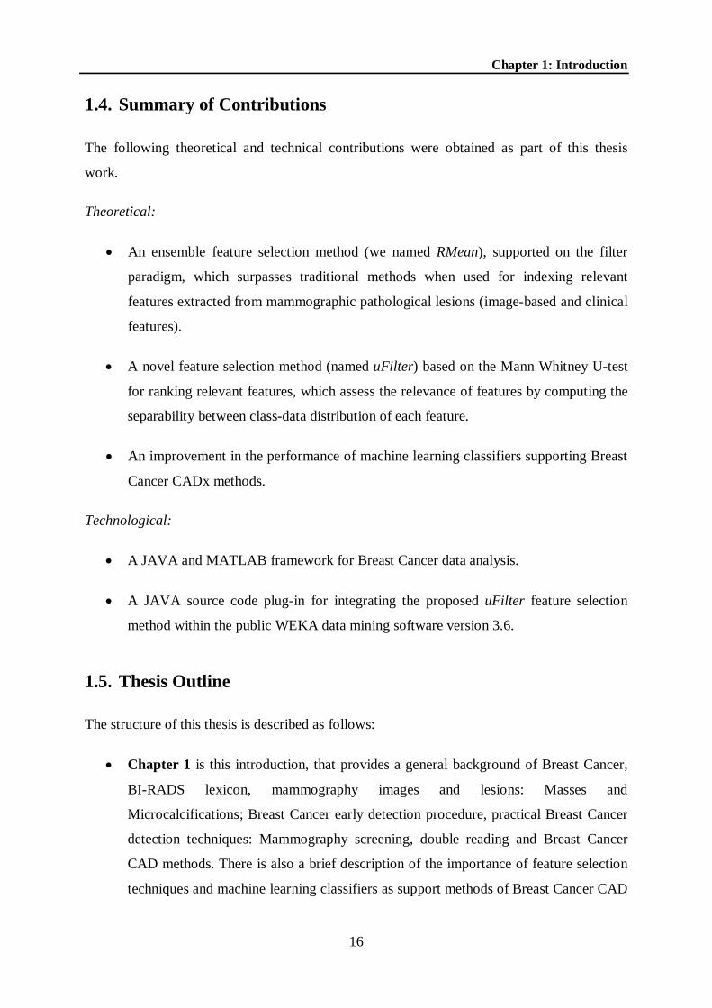
1.4. Summary of Contributions
The following theoretical and technical contributions were obtained as part of this thesis
work.
Theoretical:
An ensemble feature selection method (we named RMean), supported on the filter
paradigm, which surpasses traditional methods when used for indexing relevant
features extracted from mammographic pathological lesions (image-based and clinical
features).
A novel feature selection method (named uFilter) based on the Mann Whitney U-test
for ranking relevant features, which assess the relevance of features by computing the
separability between class-data distribution of each feature.
An improvement in the performance of machine learning classifiers supporting Breast
Cancer CADx methods.
Technological:
A JAVA and MATLAB framework for Breast Cancer data analysis.
A JAVA source code plug-in for integrating the proposed uFilter feature selection
method within the public WEKA data mining software version 3.6.
1.5. Thesis Outline
The structure of this thesis is described as follows:
Chapter 1 is this introduction, that provides a general background of Breast Cancer,
BI-RADS lexicon, mammography images and lesions: Masses and
Microcalcifications; Breast Cancer early detection procedure, practical Breast Cancer
detection techniques: Mammography screening, double reading and Breast Cancer
CAD methods. There is also a brief description of the importance of feature selection
techniques and machine learning classifiers as support methods of Breast Cancer CAD

Chapter 1: Introduction
17
systems. Finally, we describe the context that motivated the development of this
thesis, its objectives and summarized its contributions.
Chapter 2 describes the current state of the art of the principal topics related to the
proposed objectives: (1) Breast Cancer supporting repositories, (2) Clinical and image-
based descriptors for Breast Cancer, (3) A comprehensive explanation of feature
selection methods: the most important feature selection paradigms, the main
algorithms, as well as advantages and disadvantages of them, (4) A detailed
description of the most used Breast Cancer machine learning classifiers and (5) CAD
methods in Breast Cancer, which surveys several successful CADe and CADx
systems, involving methods and techniques used for detection/classification of
microcalcifications and masses.
Chapter 3 details the experimental methodologies used in this thesis, such as: datasets
description; the elected clinical and image-based descriptors; exploration of machine
learning classifiers and features selection methods. We also present the description
and experimental evaluation of the RMean feature selection.
Chapter 4 addresses the theoretical description and experimental evaluation of the
proposed uFilter method. We introduce a formal framework for understanding the
proposed algorithm, which is supported on the statistical model/theory of the non-
parametric Mann Whitney U-test. In addition, a software prototype implementation of
the uFilter method using these theoretical intuitions is presented.
Chapter 5 presents the conclusions of this thesis and outlines the future lines of work
opened by its contributions.

Chapter 1: Introduction
18
1.6. Auto-Bibliography
This Thesis is based primarily on the following publications:
Chapter 3:
"Ensemble features selection method as tool for Breast Cancer classification", in
Advanced Computing Services for Biomedical Image Analysis. International Journal
of Image Mining, InderScience, 2015. (Accepted)
"Improving the performance of machine learning classifiers for Breast Cancer
diagnosis based on feature selection", in Proceedings of the 2014 Federated
Conference on Computer Science and Information Systems. M. Ganzha, L.
Maciaszek, and M. Paprzycki (Eds.), IEEE, Warsaw, Poland, 2014, pp. 209-217.
http://dx.doi.org/10.15439/2014F249.
“Improving Breast Cancer Classification with Mammography, Supported on an
Appropriate Variable Selection Analysis”, Proc. SPIE 8670, Medical Imaging 2013:
Computer-Aided Diagnosis, 867022 (February 26, 2013);
http://dx.doi.org/10.1117/12.2007912
“Evaluation of Features Selection Methods for Breast Cancer Classification”,
ICEM15: 15th International Conference on Experimental Mechanics, FEUP-
EURASEM-APAET, Porto/Portugal, 22-27 July 2012. ISBN: 978-972-8826-26-0.
Chapter 4:
"Improving the Mann–Whitney statistical test for feature selection: An approach in
breast cancer diagnosis on mammography", Artificial Intelligence in Medicine, 2015,
vol. 63, no. 1, pp. 19-31. http://dx.doi.org/10.1016/j.artmed.2014.12.004.

Chapter 1: Introduction
19
Other Related Publications:
“Grid Computing for Breast Cancer CAD. A Pilot Experience in a Medical
Environment”, In 4rd Iberian Grid Infrastructure Conference Proceedings. 2010: p.
307-318. Netbiblo, 2010. ISBN: 978-84-9745-549-7.
“Grid-based architecture to host multiple repositories: A mammography image
analysis use case”, Ibergrid: 3rd Iberian Grid Infrastructure Conference Proceedings,
2009: p. 327-338. Netbiblo, 2009. ISBN: 978-84-9745-406-3.
“A CAD Tool for mammography image analysis. Evaluation on GRID environment”,
in 3º Congresso Nacional de Biomecânica. 2009. Bragança, Portugal: Sociedade
Portuguesa de Biomecânica. pp. 583-589. ISBN 978-989-96100-0-2.

20
State of the Art
Among several research areas covered by the Breast Cancer CAD systems, in this chapter it is
made a revision of critical topics, such as: (1) Breast Cancer supporting repositories, which
presents a brief description of a wide range of publicly accessible breast cancer repositories;
(2) Clinical and image-based descriptors for Breast Cancer that outlines several important
image-based features extracted from detected pathological lesions on mammography images;
(3) Feature selection methods, which describes the most important feature selection
paradigms, the algorithms, as well as advantages and disadvantages of them; (4) Machine
learning classifiers from the radiologists point of view, thus, it is addressed the most used
classifiers employed in Breast Cancer detection/classification; and (5) CAD methods in Breast
Cancer, this section surveys several successful CADe and CADx systems, their methods and
techniques used for detection/classification of MCs and masses.
CH
AP
TER

Chapter 2: State of the Art
21
2.1. Breast Cancer Supporting Repositories
Currently, there are numerous Breast Cancer databases available to the research community,
some public and others private - restricted to particular institutions (i.e. the massive database
provided by the National Digital Medical Archive Inc, USA, that holds over a million
mammography images [105]). Although the increasing effort of different research groups into
satisfy different aspects of the ideal Breast Cancer database (more simple and well
documented), each database is unique; not only are the cases different or the proportion of
subtle cases versus obvious cases are different, more importantly, often do not contain all the
requirements needed for a research purpose [106-110]. Therefore, different databases have
different strengths and weaknesses. Due to this, it is very difficult to compare the performance
of different algorithms, methods and techniques as well as to determine which would be the
most useful. The Breast Cancer Digital Repository (BCDR) [30], the Mammographic Image
Analysis Society (MIAS) database [111] and the Digital Database for Screening
Mammography (DDSM) [112] are easily accessed databases and thus they are considered the
most commonly used databases in the scientific community.
The BCDR which is the first Portuguese breast cancer image database, with anonymous cases
from medical records supplied by the Faculty of Medicine “Centro Hospitalar São João” at
University of Porto, Portugal [30]. BCDR is composed of 1730 patient cases with
mammography and ultrasound images, clinical history, lesion segmentation and selected pre-
computed image-based descriptors, for a total of 5776 images. Patient cases are classified
using the BI-RADS classification and annotated by specialized radiologists (276 biopsies
proven at the time of writing).
The MIAS database [111] is formed by 322 Mediolateral-Oblique (MLO) mammography
image view. In this database, the image files are available in PNG (portable network graphics)
format with a resolution of 1,024 x 1,024 pixels, which are also annotated with the following
information: a database reference number indicating left and right breast, character of
background tissue, pathology, class of lesion present and coordinates as well as size of these
lesions.
The DDSM database [112] is the largest public database. Officially contains 2479 cases
including two images of each breast, acquired in Craniocaudal (CC) and MLO views that
have been scanned from the film-based sources by four different scanners with a resolution

Chapter 2: State of the Art
22
between 50 and 42 microns, for a total of 9916 images with all types of findings (normal,
benign and malign cases). These images are coded according to the Lossless Joint Pictures
Expert Group (LJPEG) standard format and its conversion is necessary before using it.
Besides, there are more recent public developed projects of mammographic image databases.
All of them available after the web-accessible registration: The BancoWeb LAPIMO
(acronym of “Laborátorio de Análise e Processamento de Imagens Médicas e
Odontológicas”) Database [113] it is a public repository which contains 320 cases, 1473
images (MLO and CC views) divided in normal images, and images with benign and malign
findings. Also background patient information along with BI-RADS annotations is available.
The INbreast database [114] contains a total of 115 patient cases representing 410 images
(MLO and CC) provided by the Breast Center located at the “Centro Hospitalar de São João,
Porto” and in compliance with the Portuguese National Committee of Data Protection and
Hospital’s Ethics Committee. The images files are FFDM with a solid contrast resolution of
14 bits acquired by a MammoNovation Siemens scanner. As a ground truth, all annotations
were based on the lesions contour made by specialists.
The Image Retrieval in Medical Applications (IRMA) project [115, 116] is an integration of
four mammographic databases in which standardized coding of tissue type, tumor staging,
and lesion description was developed according to the ACR tissue codes and the BI-RADS.
IRMA database is containing 10,509 reference images divided into three categories: normal
cases (12 volumes), cancer cases (15 volumes) and benign cases (14 volumes); each case may
have one or more associated Pathological Lesions (PLs) segmentations, usually in MLO and
CC images of the same breast.
The Dr. Josep Trueta [117] is a non-public database, which contains 320 images files
representing both the MLO and CC image view of 89 archived patient cases. All images were
acquired using a Siemens Mammonat Novation scanner with a resolution of 70 microns (12-
bits contrast resolution) and two different image sizes depending on the breast size are
included: 2560 x 3328 or 3328 x 4096 pixels. The ground truth is based on the center and
radius of the circle surrounding the selected ROI (all kind of lesions).
The Nijmegen [106, 118] database is widely used by researchers developing computerized
methods for detecting clustered Microcalcifications in mammograms. It is composed by 40
images belonging to 21 patient cases acquired from the National Expert and Training Centre
for Breast Cancer Screening and the Department of Radiology at the University of Nijmegen,
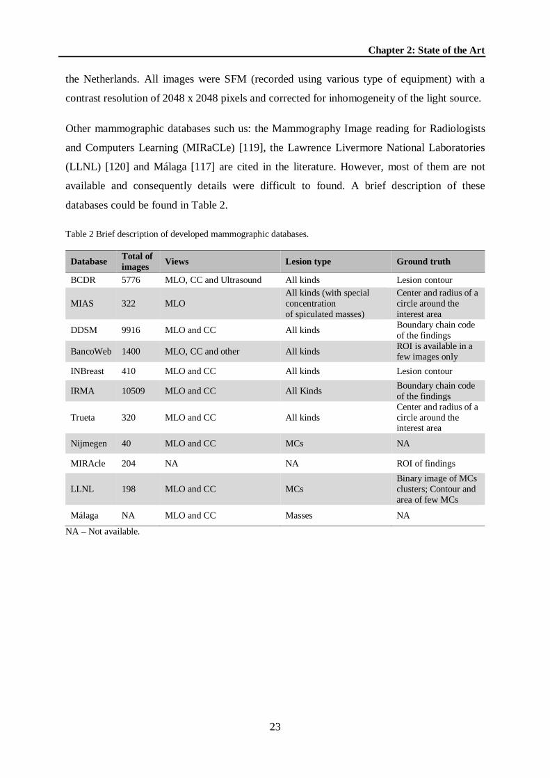
Chapter 2: State of the Art
23
the Netherlands. All images were SFM (recorded using various type of equipment) with a
contrast resolution of 2048 x 2048 pixels and corrected for inhomogeneity of the light source.
Other mammographic databases such us: the Mammography Image reading for Radiologists
and Computers Learning (MIRaCLe) [119], the Lawrence Livermore National Laboratories
(LLNL) [120] and Málaga [117] are cited in the literature. However, most of them are not
available and consequently details were difficult to found. A brief description of these
databases could be found in Table 2.
Table 2 Brief description of developed mammographic databases.
Database Total of images Views Lesion type Ground truth
BCDR 5776 MLO, CC and Ultrasound All kinds Lesion contour
MIAS 322 MLO All kinds (with special concentration of spiculated masses)
Center and radius of a circle around the interest area
DDSM 9916 MLO and CC All kinds Boundary chain code of the findings
BancoWeb 1400 MLO, CC and other All kinds ROI is available in a few images only
INBreast 410 MLO and CC All kinds Lesion contour
IRMA 10509 MLO and CC All Kinds Boundary chain code of the findings
Trueta 320 MLO and CC All kinds Center and radius of a circle around the interest area
Nijmegen 40 MLO and CC MCs NA
MIRAcle 204 NA NA ROI of findings
LLNL 198 MLO and CC MCs Binary image of MCs clusters; Contour and area of few MCs
Málaga NA MLO and CC Masses NA
NA – Not available.

Chapter 2: State of the Art
24
2.2. Clinical and Image-based Descriptors for Breast Cancer
2.2.1. Clinical Descriptors
According to the ACR, which is the copyright owner of the BI-RADS Atlas, clinical
descriptors are related to morphological description, distribution and location of pathological
lesions in mammography images [7]. These descriptors were selected on the basis of their
ability to discriminate between benign and malignant findings and represent the patient
associated metadata.
There are three morphological categories to describe breast lesions: focus/foci, mass and non-
mass-like enhancements (calcifications in most cases). A focus/foci is a breast lesion smaller
than 5 mm. A mass is a lesion characterized by the shape, which can be round, oval lobulated
and irregular; the margin, which could be obscured, irregular and speculated and, the internal
mass enhancement characteristics such as: homogeneous, heterogeneous, rim enhancement,
dark internal septations, enhancing internal septatios, and central enhancement. The non-mas-
like enhancement category is characterized by different distribution patterns: focal, linear,
ductal, segmental, regional, multiple regions and diffuse. Furthermore, the distribution
patterns can be defined by internal characteristics, which includes homogeneous,
heterogeneous, stippled/punctate, clumped and reticular/dendritic, and whether the
enhancement is symmetric or asymmetric between both breasts [7].
The location of the lesion is described using the clinical orientation extrapolated from the film
location where the patient’s breast is considered the face of a clock facing the observer
(radiologist). The first option to describe the location is the uses of quadrants (upper outer
quadrant, upper inner quadrant, lower outer quadrant and lower inner quadrant). The
utilization of both the clock face (left or right or both for side) and quadrants provides an
internal consistency check for possible right-left confusion. Usually, the side is given first,
followed by the location and depth (anterior, middle and posterior) of the lesion. The location
of the lesion under and behind the nipple are considered subareolar and central regions
respectively [7].
Furthermore, the inclusion of a statement describing the general breast tissue type arose from
evidence in the literature establishing that increased breast density is accompanied by

Chapter 2: State of the Art
25
decreased sensitivity. There is good evidence that increased breast density also is related with
increased risk of breast cancer [121, 122]. Thus, the inclusion of four categories describing
the breast density in the standard mammography report improves the communication of
predicted mammographic performance and breast cancer risk [7].
Sometimes, a finding cannot be adequately described by a single descriptor. This is often true
with calcification lesions and its margin characteristics. Calcifications may include several
different types (punctate and amorphous); if one type predominates, a single descriptor may
be the best; if not, multiple descriptors may be preferred [7]. For example, the work of
Burnside et al [123] evaluates MCs descriptors (distribution or morphology) to help stratify
the risk of malignancy. The study used a population of 115 women cases and the Fisher exact
test was performed to determine significant difference between each descriptors. As result,
each calcification descriptor was able to help stratify the probability of malignancy as follows:
coarse heterogeneous (7%), amorphous (13%), fine pleomorphic (29%), and fine linear
(53%).Also, the statistical test of Fisher revealed a significant difference among these
descriptor categories (p = 0.005).
The same flexibility should be considered when describing masses margins. Sometimes, they
could be partially obscured by surrounding glandular tissue. If the margin is at least 75%
circumscribed and 25% obscured, the mass can be classified according to its circumscribed
margin. In opposite, if the margin is partially circumscribed and partially indistinct, the
classification will be on the basis of its indistinct margins [7].
Clinical descriptors presented in the BI-RADS lexicon constitute a quality assurance tool
reducing confusion in breast imaging interpretations [7, 124]. Moreover, recently researches
have been using combinations of clinical and image-based descriptors for improving the
breast cancer classification performance [75, 88].
2.2.2. Image-based Descriptors
Breast abnormalities present varying diagnostic information on mammograms. The diagnostic
features vary in terms of shape, density, texture and distribution. Many studies therefore have
focused on analyzing extracted image-based descriptors from MCs and masses on
mammographic. An overview of most employed group of image-based descriptors for MCs
detection/classification could be observed in Table 3.
Chapter 2: State of the Art
26
Mammographic Microcalcifications Descriptors
According to the clinician procedure of radiologists, MCs clusters can be characterized by its
morphology and location, the morphologies of the individual calcification particles, and the
distribution of the particles within the cluster. Different approaches for automatic
characterization of calcifications simulate the radiologists’ strategy, and hence, four principal
classes of features for the discrimination of MCs clusters can be defined: features based on the
morphology and location of the cluster, morphology-based features of individual
microcalcification particles, features based on the spatial distribution and optical density of
the individual particles within the cluster, and texture-based features of the MCs surrounding
background tissue [125].
Morphology and Location of Microcalcifications Clusters
Several researchers considered the representation of the cluster shape based on the calculation
of the convex hull of the centroids or the contour pixels of the particles in a cluster. From this
shape representation, a set of descriptors such as: area, perimeter, circularity, rectangularity,
orientation, eccentricity and normalized central moments can be computed. Another important
feature that describes the morphology of a MCs cluster is the number of individual
calcification particles in the cluster. This feature is very often employed for the
characterization of MCs clusters and can easily be obtained from a segmentation of the
individual MCs [28, 77, 86, 126]. Also, the MC coverage, which is defined by the ratio of the
sum of the individual MC areas and the cluster area, is used to describe how densely packed a
cluster is with MCs.
The location of the MCs cluster is another important aspect to be considered when analyzing
the probability of malignancy of a breast lesion. According to the ACR, malignant lesions are
more often located in the upper outer quadrant than other quadrants of the breast [7]. Hence
several approaches prefer the computation of location-based features of the MCs clusters in
the mammogram. For example in [86], It was used the relative distance of a cluster to the
pectoral muscle and the breast edge as discriminative features. It is important to note that
extracting features based on the location usually require a robust segmentation method for
structures like the nipples, pectoral muscle, and breast boundary in the mammograms, which
is a complex problem.

Chapter 2: State of the Art
27
Morphology of an Individual Microcalcification
Usually, a set of statistics features such as: mean, standard deviations, minimum, maximum,
or median are computed from an individual MC in a cluster. Many approaches considered the
computation of the mean and standard deviations from previously computed shape descriptors
like the areas, perimeters, circularities, rectangularities, orientations, and eccentricities of the
MCs [77, 78, 86, 110, 126-128]. Also, the means and standard deviations of the individual
normalized central moments as well as of the moments of the border pixels are used by some
researchers [78, 126, 129, 130].
Veldkamp and Karssemeijer [86] employed a set of 16 image-based (intensity and shape)
descriptors extracted from MCs lesions on ipsilateral images view (MLO and CC). The AUC-
based classification performance of the kNN classifier was 0.83 for a dataset of 90 patient
cases. Kallergi [126] employed 13 image-based descriptors extracted from the morphology of
individual MCs and the distribution of the clusters. The best result was obtained when
including the patient’s age as input in the classification scheme, achieving an AUC of 0.98.
Zhang et al. [73] used two categories of features extracted from MCs in a two-step procedure
to reduce the false positive rate. The set of descriptors included spatial and morphological
features: average gray level of the foreground and background, standard deviation of the gray-
level of the foreground and background, compactness, moment, and Fourier descriptor. Also,
features related to the MCs cluster were added to the set of features. In the first step of the
detection procedure was used only MCs features to reduce the false detection. In the second
step were included two more MCs clusters features (cluster region size and cluster shape rate)
to reduce the false detection rate. Experimental results using a back-propagation neural
network showed that the method could reduce the false detection rate by 42% (3.15 per
image).
Leichter in [131] analyzed the influence of two type of features in the diagnostic role. The
selected features were: eccentricity (reflecting the geometry of clusters) and, the shape factor
and number of neighbors (reflecting the shape of the individual MC). The analysis was
performed using a dataset formed by 324 clustered of MCs (with biopsy-proven). According
to the obtained classification result (AUC value of 0.87) by a linear discriminant analysis, it
was possible to conclude that the cluster geometry feature was more effective in
differentiating benign from malignant clusters than was the shape of individual MC.

Chapter 2: State of the Art
28
Chan et al [132] compared two set of MCs features (morphological and texture) for
discriminating between benign and malignant lesions. Morphological descriptors were related
to size, contrast, shape of MCs and their variations within clusters. Meanwhile, texture
descriptors were all derived from the spatial grey-level dependence matrices constructed at
different distances and directions. The combined morphological and texture features achieved
an AUC of 0.89, which increased to 0.93 when averaging discriminant scores from all views
of the same cluster. This result was superior when comparing with the obtained result by
using morphological features (0.79) or texture features (0.84) alone.
Spatial Distribution and Optical Density of Microcalcifications
Two of the most employed features for describing the spatial distribution of MCs inside a
cluster are the mean and standard deviation of the computed distances between individual
MCs [84, 133]. Other interesting features but used in less degree are the eccentricity and the
normalized central moments of the MC centroids. The research of Leicheter [134] describes a
more complex scenario for using the mean as a spatial distribution feature. In this case is used
the two-dimensional Delaunay triangulation of the MCs centroids for obtaining the k-number
of nearest neighbors of the MCs inside the cluster, then, the mean of these k-neighbors is
obtained. In others approaches, the mean and variance of grey values and the contrast of
individual MCs have been employed for describing the optical density of MCs [77, 86, 129,
133].
Texture of Microcalcifications
The texture features based on the Haralick's descriptors constitute a powerful set of image-
based features, which have been widely used for describing MCs lesions [78, 84, 129, 132,
135-137]. They are extracted from the Gray-Level Co-occurrence Matrices (GLCM) and
represent the second-order statistics of the grey levels in a ROI [138]. Also, the texture
analysis based on the wavelet descriptors has demonstrated to be important for MCs
characterization [84, 129].
Dhawan et al [84] used two set of texture features extracted from GLCM and wavelet from
ROIs containing MCs lesions. They reported an obtained AUC of 0.86 in the classification of
191 “difficult to diagnose” cases. Soltanian-Zadeh et al [129] compared the performance of
four features sets (GLCM based, shape, wavelet and multiwavelet features); the multiwavelet

Chapter 2: State of the Art
29
features, which use multiple scaling functions and mother wavelets outperformed the other
three features sets, achieving an AUC of 0.89.
Mohanty et al [137] proposed a new system for breast cancer classification based on the
technique of the association rule mining. The system used a set of 26 features extracted from
the first and second-order statistics of MCs lesions. These features were enough (according to
the minimization of the classification error) for differentiating between normal and cancerous
breast tissues.
Malar et al [70] used three different set of features extracted from the GLCM, Gabor filter
bank and wavelet transformation, for the discrimination of MCs from the normal tissue. The
method was validated using a dataset formed by 120 ROIs containing normal and MCs
images. The results highlighted that extreme machine learning produced better classification
accuracy (94%) when using wavelet features.
Yu et al. in [139] presented a two-stage method for detecting MCs in digital mammograms.
The first stage used a wavelet filter according to the mean pixel value for the detection of
MCs. Subsequently, in the second stage is used a Markov random field model to extract
textural features from the neighborhood of every detected calcification. These textural
features in combination with other three auxiliary features (the mean pixel value, the gray-
level variance, and a measure of edge density) were used as inputs for both the Bayes and
Feed Forward Back-Propagation (FFBP) neural network classifiers. The method was
evaluated using 20 mammograms containing 25 areas of clustered MCs. As results, the
method was able to reject false positive in a 98.9% of the cases with a sensitive of 92%, at
0.75 false positive per image.
AbuBaker et al. in [140] presented a study of the characteristics of true MCs compared to
falsely detected MCs using first (mean, entropy, standard deviation, moment3, kurtosis) and
second (angular second moment, contrast, absolute value, inverse difference, entropy,
maximum probability) order statistical texture analysis techniques. These features were
generated with the intention of reducing the false positive ratio on mammogram images. As
result, it can successfully reduce the ratio of false positives by 18% without affecting the ratio
of true positives (currently 98%).
The application of fractal geometry for MC analysis in mammography images have been also
reported in the literature [141-143]. Its applicability is justified by the fact of being the MCs

Chapter 2: State of the Art
30
clusters tiny bright spots with different size and shape embedded in a non-homogeneous
background surrounding of breast tissue. This particular situation allows the opportunity of
using fractal geometry analysis by considering the MCs cluster as a fractal normal
background superimposed by a non-fractal foreground [144, 145].
Rangayyan and Nguyen in [143] demonstrated that the computation of the fractal dimension
of MCs contours based on the grid method facilitates the discrimination between benign and
malignant clusters. Also, the efficiency was superior when comparing with other shape factor
methods such as: compactness, the spiculation index, fractional concavity, Fourier factor.
Table 3 Overview of most employed group of image-based descriptors for MCs detection/classification.
Descriptors Description References
Individual MC features
Features extracted from mammogram directly such as perimeter, area, compactness, elongation, eccentricity, thickness, orientation, direction, line, background, foreground, distance, and contrast. They are easy to extract and they originate from the experience of radiologists.
[58, 73, 75, 77, 86, 129, 132, 137, 146-149]
Grey Level Co-occurrence Matrix features
Features extracted from GLCM. [70, 75, 78, 84, 129, 132, 135, 137, 140]
Wavelet features Energy, entropy, and norm extracted from the wavelet transform sub-images.
[70, 84, 129, 139, 150, 151]
Border information features
Features extracted from MCs border information. [78, 126, 129, 130]
Fractal dimension Features extracted from fractal model of the image [76, 141-145, 152-154]
Cluster features Features used to describe the distribution of the MCs; area, perimeters, circularity, rectangularity, orientation, and eccentricity.
[77, 78, 86, 126-128, 133, 134, 155]
Mammographic Masses Descriptors
Similar to MCs lesions, most approaches to the feature extraction for mammographic masses
are based on the lesion attributes that are used by radiologists in the clinician procedure. They
characterize masses based on their shape (also called morphological or geometrical features),
the characteristics of their margin, and their texture [7]. The standard approach is to compute
margin, shape, and texture related features from the mass and its surrounding tissue and use
them as inputs to a classifier to obtain a malignancy score. An overview of most employed
group of image-based descriptors for masses detection/classification is shown in Table 4.

Chapter 2: State of the Art
31
Shape and Margin of Masses
Most benign masses are homogeneous and possess well-defined edges; malignant tumors
typically have fuzzy or ill-defined boundaries. Benign masses possess smooth, round, or oval
shapes with possible macrolobulations, as opposed to malignant tumors which typically
exhibit rough contours with microlobulations, spiculations, and concavities (see Figure 6) [7,
156]. Based on the segmentation of the mass contour, several studies have therefore focused
on analyzing the margin and shapes of mammographic masses [28, 81, 157-159]. Similar to
the approaches used to represent the morphology of individual Microcalcification particles;
these include the area and the perimeter as well as the circularity, rectangularity, orientation,
and eccentricity of the mass.
Figure 6 Characteristics of shape and margins of masses.
Rojas and Nandi [160] developed a mass classification method based on two automated
segmentation methods: the dynamic programming based boundary tracking and constrained
region growing. They simplified the initial mass contours (after segmented) by modelling the
set of points as ellipses. Subsequently, a total of six features describing the mass margins
were extracted for further classification. The features were: contrast between foreground and
background regions, the variation coefficient of edge strength, two measures of the fuzziness

Chapter 2: State of the Art
32
of mass margins, a measure of spiculation based on relative gradient orientation, and a
measure of spiculation based on edge-signature information. As results, it was found there is a
difference of 14% in the segmentation accuracy and a 4% of difference in the classification
performance between both methods. Also, it was observed that the spiculation feature (based
on edge-signature information) was clearly better than the remaining features; however, this
feature is sensible to changes in the quality of the segmentation.
In [161], Liu et al. proposed a method for mass classification based on the combination of the
level set segmentation and shape analysis. The method used as starting point the initial mass
contour made by radiologists as input to the level set segmentation method in order to obtain
the final contour. Then, a set of shape features were extracted from the segmented masses for
further classification using the LDA and SVM classifiers. The evaluation of 292 ROIs from
DDSM mammogram images highlighted the best area under the ROC curve of 0.8803 when
using the Fourier descriptor of normalized accumulative angle feature.
Rangayyan et al. in [107] introduced two new shape factors, spiculation index and fractional
concavity, and applied them for the classification of manually segmented mammographic
masses. The combined use of the spiculation index, fractional concavity, and compactness
yielded a benign-versus-malignant classification accuracy of 81.5%. Similar approach was
presented by Guliato et al. [24], which developed a method that preserve the details of
spicules and diagnostic by generating polygonal models of contours. The classification
performance used a set of 111 contours representing 65 benign and 46 malignant masses was
an AUC value of 0.94.
Zheng and Chan in [92] proposed an algorithm for masses detection based on the combination
of several artificial intelligence methods. First, the fractal analysis was performed for the
initial selection of suspicious regions. Then, it is applied a multi-resolution Markov random
field algorithm for lesions segmentation. Finally, a classification based on the lesions shape is
performed for reducing the proportion of false positive. The obtained results on 322 images
from the Mini-MIAS databases highlighted a sensitive value of 97.3% with a 3.9 false
positives per image.
Furthermore, features based on the normalized radial length and the normalized chord length
has been used to represent the mass shape [79, 80, 85]. The normalized radial length is
defined as the Euclidean distance of each pixel on the object contour to the object’s centroid.

Chapter 2: State of the Art
33
Meanwhile, the definition of the normalized chord length is defined as the Euclidean distance
of pair of points on the object boundary.
Besides, in Zheng et al. [85] two features for describing masses margin have been proposed.
The features are: the standard deviation and the skewness of the gradient strength of the mass
contour. Spiculated margins are a symptom of malignant masses, thus, the texture analysis on
bands close to the margin of a segmented mass is important. This idea is extended in the
approach of Shi et al. [23], they developed a new feature (margin abruptness) that measures
the margin sharpness by using line detection in rubber-band-straightening transform images.
Moreover, in Mudigonda et al. [162] is proposed two features (to measure the sharpness)
based on the image gradient in a band of pixels surrounding the mass contour.
Varela et al. [27] proposed a new method for describing the mass margins in order to improve
the binary (benign and malignant) classification performance. The mass margin features used
by this method aims to measure the sharpness of the margin and the presence of
microlobulations. The AUC-based results using a dataset formed by 1076 biopsy proved
masses from the DDSM database were 0.69, 0.76 and 0.75 for interior, border and outer mass
segment respectively. Moreover, the classification performance using a combination of mass
segments (interior, border and outer) was 0.81 for image-based and 0.83 for case-based
evaluation. In this research was concluded that sharpness features perform better than
microlobulation features for masses classification.
Huo et al [74] used a set of features extracted from the margins and density of masses for
feeding three different machine learning classifiers. The best result (AUC value of 0.94) was
obtained by using a hybrid method consisting of a step rule-based method with a spiculation
measure followed by an ANN on a dataset formed by 95 masses. In another experiment, the
same classification model was employed on a dataset of 110 masses and it attained an AUC
value of 0.82 [163].
Texture of Masses
Similar to feature extraction for MCs, features based on the GLCM, gray-level run length
metrics and wavelet decompositions have been popular for the characterization of masses [27]
[162] [76, 164, 165]. However, in contrast to the diagnosis of MCs, in mass approaches, the

Chapter 2: State of the Art
34
texture analysis is not always performed on the entire ROI; sometimes the analysis is carried
out on a particular region within the ROI i.e. on bands of pixels close to the mass margin.
Mudigonda et al in [162] used texture features and two gradient-based measures to estimate
the sharpness of a mass contour. On a database of 53 mass lesions they obtained AUC values
of 0.73, 0.84 and 0.80 for sharpness, texture and combined feature spaces, respectively.
Wei et al. in [28] proposed a method for masses detection based on the combination of the
gradient field analysis and the grey level information. The method used a clustering-based
region growing algorithm for detecting the suspicious lesions. Then, a set of shape and texture
descriptors were computed from detected lesions before feeding two MLCs: ruled-based and
LDA. The reported case-based sensitive result on a mass (containing 110 cases) dataset, non-
mass (containing 90 cases) dataset and a combination of them was 70%, 80%, and 90% at
0.72, 1.08 and 1.82 false positive per image respectively.
Bellotti et al. in [71] proposed a three-stage system for mass detection. In the first stage, a
segmentation algorithm using a dynamical threshold is applied for detecting suspicious
lesions. Then, a set of eight texture features (extracted from the GLCM at different angles)
were computed from segmented lesions. In the last stage, a FFBP neural network classifier
(trained with the gradient descent learning rule) was used for discriminating between normal
masses and normal tissues. The system evaluation using a dataset containing 3369
mammography images (2307 negative cases and 1062 positive cases) reported an AUC-based
classification performance of 0.783 (standard deviation of 0.008) by the proposed system.
Sahiner et al. in [80] combined morphological and texture features for describing mass
lesions. The obtained classification results using a dataset formed by 249 images were an
AUC value of 0.83, 0.84, and 0.87 when using morphological, texture, and a combination of
both type of features respectively.
Alto et al. in [166] analyzed several image-based features in order to select masses lesions
with similar constitution in terms of computed descriptors. The evaluation of the method was
using the retrieval precision as a performance measure. The higher result (91%) was obtained
when using the three most-effective features (fractional concavity, acutance and sum of
entropy).
Mavroforakis et al. in [76] proposed a quantitative approach for masses classification by using
linear and non-linear classification architectures. Also, the method is supported by the fractal
analysis (calculated by the box-counting method) of the set of extracted texture features. The

Chapter 2: State of the Art
35
evaluation on two datasets containing 130 digitized mammograms revealed that the best score
(83.9%) was obtained by the SVM classifier using only texture features.
Ayres and Rangayyan [167-169] presented a method that analyzes the oriented texture on
mammography images in order to detect architectural distortion. The method used the Gabor
filters for obtaining the orientation field of the images and three maps models (node, saddle
and spiral) for locating the place of the architectural distortion, being the node map the most
prominent. The method was tested on two set of images, one containing 19 cases of
architectural distortion and 41 normal mammograms, and the other containing 37 cases with
architectural distortion. Sensitivity rates of 84% and 81% at 4.5 and10 false positives per
image were reported for the two set of images respectively.
More recently, Moura and Lopez in [88] developed a new round-shape descriptor based on
Histograms of Gradient Divergence (HGD) for masses classification. The HGD was
compared against eleven group of image descriptors (extracted from Intensity statistics,
Histogram measures, Invariant moments, Zernike moments, Haralick features, Grey-level run
length, Grey-level difference matrix, Gabor filter banks, Histogram of oriented gradients,
Wavelets and Curvelets) on benchmarking datasets extracted from two public available
mammography databases. Obtained results using different machine learning classifiers
revealed that the HGD was the best descriptor (or comparable to best) in 8 out of 12
scenarios, demonstrating promising capabilities to classify breast masses.

Chapter 2: State of the Art
36
Table 4 Overview of most employed group of image-based descriptors for masses detection/classification.
Descriptors Descriptions References
Intensity features
Contrast measure of ROIs; Average grey level of ROIs (Mean); Standard derivation inside ROIs or variance; Skewness and Kurtosis of ROIs; Zernike moments.
[72, 75, 88, 160, 170]
Shape features
Margin spiculation and Sharpness; Area, circularity, convexity, rectangularity and perimeter measures; Acutance measure; Shape factor; Invariant moments; Furrier descriptor; Fractal analysis.
[23, 24, 72, 75, 76, 80, 92, 107, 160-163, 166, 170, 171]
Normalized radial length and the Normalized chord length
Boundary roughness, mean, entropy, area ratio, standard deviation, zero crossing count, mean, variance, skewness and kurtosis.
[79, 80, 85, 88]
Texture features from GLCM, Grey-level difference statistics and from Run-level statistics
Energy (or angular second moment); Correlation, inertia and entropy of co-occurrence matrix; Difference moment; Inverse difference moment; Sum average, sum entropy and difference entropy; Sum variance, difference average and information of correlation; Contrast, angular second moment, entropy and mean Short and long runs emphasis, grey-level and run length non-uniformity and run percentage.
[27, 71, 72, 76, 88, 162, 164, 165]
These image-based descriptors could improve diagnostic accuracy and led to the development
of mammography-based CADx systems to increase both sensitivity and specificity [156]
2.3. Feature Selection Methods
Goal of the feature selection
The objectives of features selection are manifold, two of the most important are:
to avoid overfitting and improve model performance, i.e. prediction performance in
the case of supervised classification and better cluster detection in the case of
clustering [61, 62].
to provide faster and more cost-effective models, i.e. models with lower algorithmic
complexity [61, 62].

Chapter 2: State of the Art
37
Selection paradigms
Selecting the optimal feature subset for supervised learning problems requires an exhaustive
search of all possible subsets of features of the chosen cardinality, which is not practical in
most situations because the number of possible subsets given N features is 2N−1 (the empty
set is excluded), which means NP-hard algorithms [56]. Hence, in practical machine learning
applications, usually a satisfactory instead of the optimal feature subset is searched. Feature
selection techniques differ from each other in the way they incorporate this search in the
added space of feature subsets in the model selection.
Regarding their classification, feature selection techniques can be structured into three
paradigms, depending on how they combine the feature selection search with the construction
of the classification model: filters (univariate and multivariate), wrappers and more recently
hybrid methods. Filters methods are considered the earliest approaches to feature selection
within machine learning and they use heuristics based on general characteristics of the data
rather than a machine learning classifiers to evaluate the merit of features [56, 57]. Wrappers
methods utilize machine learning classifiers as a black box to score subsets of features
according to their predictive power. Finally, the Hybrid methods combine filter and wrapper
methods as a unique model to perform feature selection. As consequences, filter methods
generally present lower algorithmic complexity and are much faster than wrapper or hybrid
methods [56, 57].
On the other hand, feature selection methods can be also categorized depending on search
strategies used. Thus, the following search strategies are more commonly used [60, 172]:
Forward selection: start with an empty set and greedily add features one at a time.
Backward elimination: start with a feature set containing all features and greedily
remove features one at a time.
Forward stepwise selection: start with an empty set and greedily add or remove
features one at a time.
Backward stepwise elimination: start with a feature set containing all features and
greedily add or remove features one at a time.
Random mutation: start with a feature set containing randomly selected features, add
or remove randomly selected features one at a time and stop after a given number of
iterations.

Chapter 2: State of the Art
38
2.3.1. Filter Paradigm
Filter techniques assess the relevance of features by looking only at the intrinsic properties of
the data. In most cases a feature relevance score is calculated, and low-scoring features are
removed. Afterwards, this subset of features is presented as input to the classification
algorithm [56]. A generalized filter algorithm is showed in Table 5. For a given dataset D, the
algorithm starts the search by using an initial subset S0, which could be an empty set, a full
set, or any randomly selected subset through the whole feature space and according to a
particular search strategy. Subsequently, the initial subset S0 is evaluated by an independent
measure M and the result is stored in best . After that, a new features subset S is generated and
evaluated (by the same M independent measure) for further comparison with the previous best
one best . If it is found to be better, it is regarded as the current best subset. The search iterates
until a predefined stopping criterion is reached. The algorithm outputs the last current best
subset Sbest as the final result.
Table 5 Pseudocode of the generalized filter algorithm.
Filter Algorithm input:
),...,,( 110 NfffD // initial dataset with N features
0S // an empty subset to start the search
// a stopping criterion output:
bestS // an optimal subset of features
begin );,( 0 MSevalbest // evaluate 0S by an independent measure M
do begin );(DgenerateS // generate a subset of feature for evaluation
);,,( MDSeval // evaluate the current subset S by an independent measure M
if ( best )
;best
;SSbest
end until ( is reached); return ;bestS
end
From this algorithm, it is possible to vary the search strategies (S) and evaluation measures
(M) to design different individual filter models. Since the filter models are independent of any
classifiers, it does not inherit any bias and will be computationally efficient.
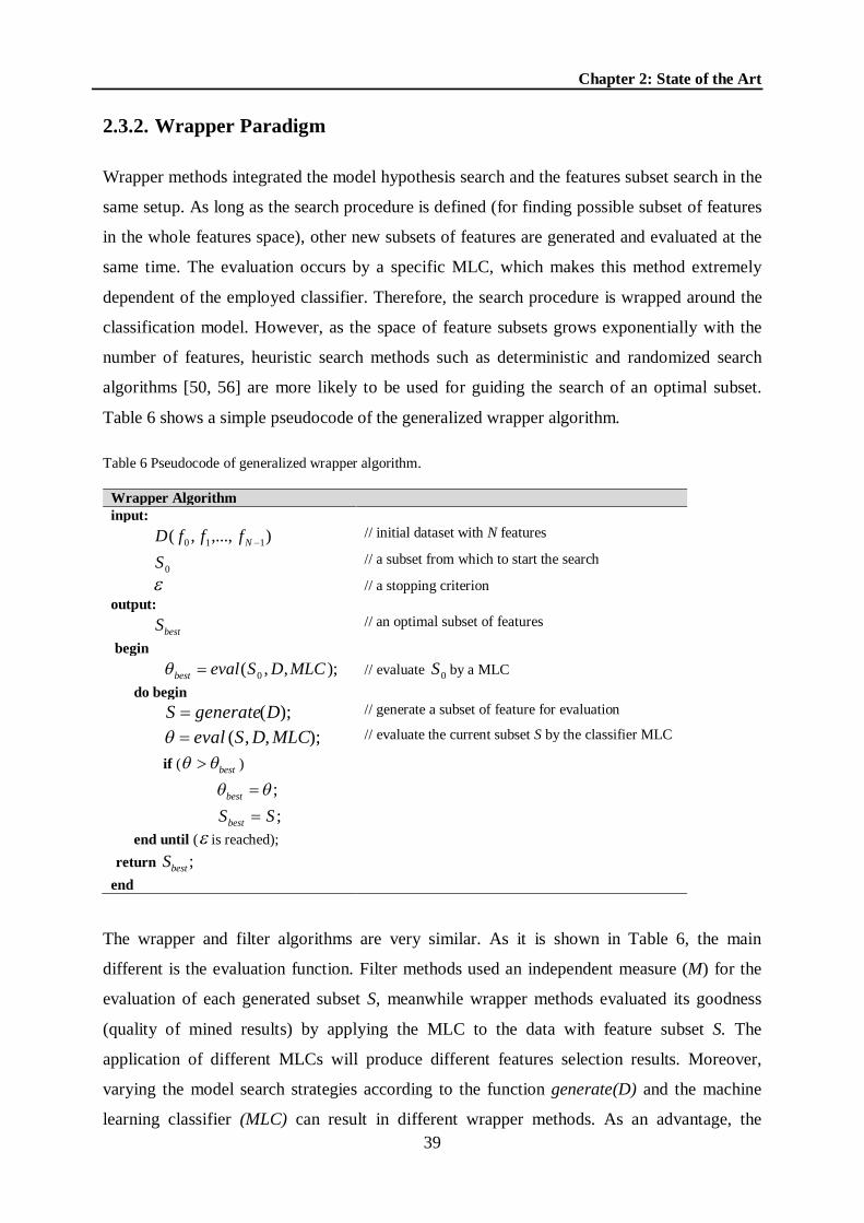
Chapter 2: State of the Art
39
2.3.2. Wrapper Paradigm
Wrapper methods integrated the model hypothesis search and the features subset search in the
same setup. As long as the search procedure is defined (for finding possible subset of features
in the whole features space), other new subsets of features are generated and evaluated at the
same time. The evaluation occurs by a specific MLC, which makes this method extremely
dependent of the employed classifier. Therefore, the search procedure is wrapped around the
classification model. However, as the space of feature subsets grows exponentially with the
number of features, heuristic search methods such as deterministic and randomized search
algorithms [50, 56] are more likely to be used for guiding the search of an optimal subset.
Table 6 shows a simple pseudocode of the generalized wrapper algorithm.
Table 6 Pseudocode of generalized wrapper algorithm.
Wrapper Algorithm input:
),...,,( 110 NfffD // initial dataset with N features
0S // a subset from which to start the search
// a stopping criterion output:
bestS // an optimal subset of features
begin );,,( 0 MLCDSevalbest // evaluate 0S by a MLC
do begin );(DgenerateS // generate a subset of feature for evaluation
);,,( MLCDSeval // evaluate the current subset S by the classifier MLC
if ( best )
; best
;SSbest
end until ( is reached); return ;bestS
end
The wrapper and filter algorithms are very similar. As it is shown in Table 6, the main
different is the evaluation function. Filter methods used an independent measure (M) for the
evaluation of each generated subset S, meanwhile wrapper methods evaluated its goodness
(quality of mined results) by applying the MLC to the data with feature subset S. The
application of different MLCs will produce different features selection results. Moreover,
varying the model search strategies according to the function generate(D) and the machine
learning classifier (MLC) can result in different wrapper methods. As an advantage, the

Chapter 2: State of the Art
40
features subset selection is supervised by the employed classifier; thus, the final subset of
features will provide better classification performances. However, this improvement has the
inconvenient that they are more computationally expensive than the filter model.
2.3.3. Hybrid Paradigm
Hybrid methods combine filter and wrapper methods as a unique model for achieving the best
performance using a particular MLC with a similar time complexity to a filter method. They
use the filter methods for obtaining information about the ranking and thus, to guide the
search for wrapper methods. These methods are more recent approach and constitute a
promising direction in the feature selection field [52].
The hybrid model is proposed to handle large datasets [173]. A general hybrid algorithm uses
an independent measure (filter method) and a MLC (wrapper method) to evaluate subset of
features (see Table 7). The independent measure (M) selects the best subset of features
according to a given cardinality and then, the MLC determines the best subset of features
among all generated subsets (with different cardinalities).
Basically, the algorithm starts the search with an empty subset S0 and tries to find the best
subsets while is increased the cardinality. For each round, the best subset with cardinality c
and the new generated subset S (by adding one feature from the remaining features) with
cardinality c+1 are evaluated using an independent measure (M) and then it is established a
comparison between them. If the S subset with cardinality c+1 is better, it becomes the
current best subset of features S'best at level c+1. At the end of each round, the S subset with
cardinality c and the new S'best subset with cardinality c+1 are evaluated by a MLC for further
comparison according to their mined result θ. If S'best is better, the algorithm continues to find
the best subset at the next level; otherwise, it stops and outputs the current best subset as the
final best subset. The quality of results from a MLC provides a natural stopping criterion in
the hybrid model.

Chapter 2: State of the Art
41
Table 7 Pseudocode of generalized hybrid algorithm.
Hybrid Algorithm input:
),...,,( 110 NfffD // initial dataset with N features
0S // a subset from which to start the search
output:
bestS // an optimal subset of features
begin );( 00 Scardc // calculate the cardinality of 0S
);,,( 0 MDSevalbest // evaluate 0S by an independent measure M
);,,( 0 MLCDSevalbest // evaluate 0S by a classifier MLC
for 10 cc to N begin
for i = 0 to N - c begin ;jbest fSS // generate a subset of feature with cardinality c for
evaluation );,,( MDSeval // evaluate the current subset S by an independent measure M
if ( best )
;best
;' SS best
end );,,'( MLCDSeval best // evaluate bestS ' by a classifier MLC
if ( best )
;'bestbest SS
; best
else break and return bestS
end return ;bestS
end
2.3.4. Related Works
Koller and Sahami [101] proposed an algorithm for feature subset selection that uses
backward elimination to eliminate predefined number of features. The idea is to select a
subset of features that keeps the class probability distribution as close as possible to the
original distribution that is obtained using all the features. The algorithm starts with all the
features and performs backward elimination to eliminate a predefined number of features. The
evaluation function selects the next feature to be deleted based on the Cross entropy measure.
For each feature the algorithm finds a subset of K features such that, the feature is
approximated to be conditionally independent of the remaining features. Setting K = 0 results

Chapter 2: State of the Art
42
in a much faster algorithm that is equal to a simple filtering approach commonly used on text-
data.
In the Relief algorithm [174] the main idea is to estimate quality of the features according to
how well their values distinguish between examples that are similar. The feature score is
calculated from a randomly selected subset of training examples, so that each example is used
to calculate the difference in the distance from the nearest example of the same class and the
nearest example of the different class. The nearest instances are found using the kNN
algorithm. Some theoretical and empirical analysis of the algorithm and its extensions is
provided in [175].
Almuallim and Dietterich [176] developed several feature subset selection algorithms
including a simple exhaustive search and algorithms that use different heuristics. They based
their feature subset evaluation function on conflicts in class value occurring when two
examples have the same values for all the selected features. In the first approach (named
FOCUS), all the feature subsets of increasing size are evaluated until a sufficient subset is
encountered. Feature subset Q is said to be sufficient if there are no conflicts i.e. if there is no
pair of examples that have different class values and the same values for all the features in Q.
The second approach (called FOCUS-2) reduces the search space by evaluating only
promising subsets. As both algorithms assume the existence of a solution (small set of
features) their application on domains with a large number of input variables can be
computationally infeasible. Due to this, heuristics searches are implemented on further
versions of the algorithm.
Aijuan and Baoying in [177] proposed a multi-resolution approach to automated classification
of mammograms using Gabor filters (with different frequencies and orientations). They
applied the statistical t-test and its p-value for feature selection and weighting respectively.
According to the experimental results, the statistical t-test reduced the feature space without
degrading the classification performance.
Akay in [178] proposed a breast cancer diagnosis method based on the combination of the
SVM classifier and the f-score feature selection method. The performance of the method is
evaluated using classification accuracy, sensitivity, specificity, positive and negative
predictive values, receiver operating characteristic curves and confusion matrix on different
training-test partitions of the Wisconsin Breast Cancer Dataset. The results show that the

Chapter 2: State of the Art
43
highest classification accuracy (99.51%) is obtained for the SVM model that contains five
features.
Aha and Bankert in [179] used a wrapper approach for feature subset selection in instance-
based learning. They proposed a new search strategy that performs beam search using a kind
of backward elimination. Namely, instead of starting with an empty feature subset, their
search randomly selects a fixed number of feature subsets and starts with the best among
them.
Recently, the work of Chandrashekarand and Sahin [180] presents a survey of feature
selection methods. They implemented the correlation criteria and mutual information methods
from the filter paradigm, the sequential floating forward selection and a modified version of
the genetic algorithm (named CHGA) methods from the wrapper paradigm. These methods
were evaluated with the performance of a SVM and radial basis function network classifiers
on seven datasets, including five from the UCI machine learning repository (Wisconsin breast
cancer dataset, Diabetes, Ionosphere, Liver Disorder and Medical).
In [181], a set of three feature selection methods were developed for combining with a
multilayer neural network and multiclass support vector machines. The developed methods
used the backward elimination and direct search in selecting a subset of salient features. Also,
in these classification models was employed the mutual information between class labels and
classifier outputs as an objective function. The methods were evaluated on various artificial
and real world datasets (including the Wisconsin Breast Cancer Diagnosis).
Lately, algorithms of the hybrid model [51, 55, 173, 182-184] are considered to handle data
sets with high dimensionality. A number of algorithms that combines fuzzy logic and genetic
programming in selecting relevant features for ANN and decision trees have been proposed
[185, 186]. Rakotomamonjy in [187] proposed new feature selection criteria derived from
SVMs and were based on the generalization error bounds sensitivity with respect to a feature.
The effectiveness of these criteria was tested on several problems including medical datasets
(Breast Cancer, Colom Cancer, Diabetes and Heart data).
Richeldi and Lanzi in [188] proposed a two-step feature selection method named ADHOC.
First, the method identifies false features according to a previous constructed profile of each
feature, then; a genetic algorithm is used for finding an important subset features. Other
studies (e.g. ref [184], [55] and [189]) also use genetic algorithms in feature selection. In

Chapter 2: State of the Art
44
[184], is combined a filter and wrapper method as a unique approach (hybrid) for feature
selection. The filter method used the mutual information to guide the searching and ranking
the features space. Then, a wrapper method based on a genetic algorithm is used for finding
the most relevant subset of features.
2.3.5. Comparative Analysis
The earliest approaches to feature selection within machine learning were filter methods.
Filter methods use heuristics based on general characteristics of the data rather than a learning
algorithm to evaluate the merit of feature subsets.
Advantages of filter techniques are that they easily scale to very high-dimensional datasets
[56], they are computationally simple and fast, and they are independent of the classification
algorithm. The process of feature selection is often most useful in situations in which
wrappers may overfit, i.e. with small training sets. As a result, feature selection needs to be
performed only once, and then different classifiers can be evaluated [173]. A common
disadvantage of filter methods is that they ignore the interaction with the classifier (the search
in the feature subset space is separated from the search in the hypothesis space), and that most
proposed techniques are univariate. This means that each feature is considered separately,
thereby ignoring feature dependencies, which may lead to worse classification performance
when compared to other types of feature selection techniques. In order to overcome the
problem of ignoring feature dependencies, a number of multivariate filter techniques were
introduced, aiming at the incorporation in some degree of feature dependencies.
Whereas filter techniques treat the problem of finding a good feature subset independently of
the model selection step. Wrapper approaches (as advantages) include the interaction between
feature subset search and model selection, and the ability to take into account feature
dependencies. But, a common drawback of these techniques is that they have a higher risk of
overfitting than filter techniques and are very computationally intensive, especially if building
the classifier has a high computational cost [60].
On the other hand, hybrid models attempt to take advantage of the two previous models by
exploiting their different evaluation criteria in different search stages. It means that hybrid
approaches improve the classification performance of filter approaches by including a specific
machine learning algorithm in the selection procedure, and improve the efficiency of wrapper
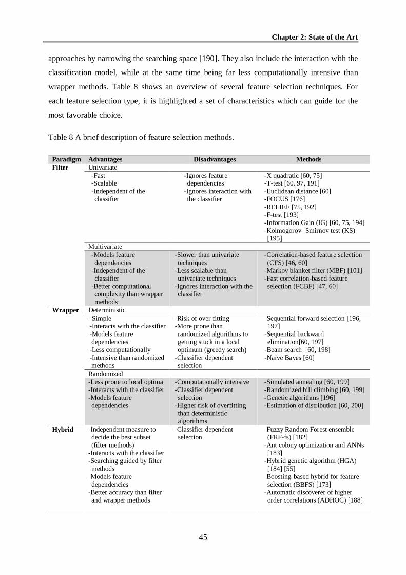
Chapter 2: State of the Art
45
approaches by narrowing the searching space [190]. They also include the interaction with the
classification model, while at the same time being far less computationally intensive than
wrapper methods. Table 8 shows an overview of several feature selection techniques. For
each feature selection type, it is highlighted a set of characteristics which can guide for the
most favorable choice.
Table 8 A brief description of feature selection methods.
Paradigm Advantages Disadvantages Methods Filter Univariate
-Fast -Scalable -Independent of the classifier
-Ignores feature dependencies
-Ignores interaction with the classifier
-X quadratic [60, 75] -T-test [60, 97, 191] -Euclidean distance [60] -FOCUS [176] -RELIEF [75, 192] -F-test [193] -Information Gain (IG) [60, 75, 194] -Kolmogorov- Smirnov test (KS) [195]
Multivariate -Models feature dependencies
-Independent of the classifier
-Better computational complexity than wrapper methods
-Slower than univariate techniques
-Less scalable than univariate techniques
-Ignores interaction with the classifier
-Correlation-based feature selection (CFS) [46, 60]
-Markov blanket filter (MBF) [101] -Fast correlation-based feature selection (FCBF) [47, 60]
Wrapper Deterministic -Simple -Interacts with the classifier -Models feature dependencies
-Less computationally -Intensive than randomized methods
-Risk of over fitting -More prone than randomized algorithms to getting stuck in a local optimum (greedy search)
-Classifier dependent selection
-Sequential forward selection [196, 197]
-Sequential backward elimination[60, 197]
-Beam search [60, 198] -Naïve Bayes [60]
Randomized -Less prone to local optima -Interacts with the classifier -Models feature dependencies
-Computationally intensive -Classifier dependent selection
-Higher risk of overfitting than deterministic algorithms
-Simulated annealing [60, 199] -Randomized hill climbing [60, 199] -Genetic algorithms [196] -Estimation of distribution [60, 200]
Hybrid -Independent measure to decide the best subset (filter methods)
-Interacts with the classifier -Searching guided by filter methods
-Models feature dependencies
-Better accuracy than filter and wrapper methods
-Classifier dependent selection
-Fuzzy Random Forest ensemble (FRF-fs) [182]
-Ant colony optimization and ANNs [183]
-Hybrid genetic algorithm (HGA) [184] [55]
-Boosting-based hybrid for feature selection (BBFS) [173]
-Automatic discoverer of higher order correlations (ADHOC) [188]

Chapter 2: State of the Art
46
2.4. Machine Learning Classifiers
In the daily practice of radiology, medical images from different modalities are read and
interpreted by radiologists. Usually radiologists must analyze and evaluate these images
comprehensively in a short time. But with the advances in modern medical technologies, the
amount of imaging data is rapidly increasing.
Machine learning provides an effective way to automate the analysis and diagnosis for
medical images. It can potentially reduce the burden on radiologists in the practice of
radiology. Bishop and Nasrabadi in [201] defined machine learning as the study of computer
algorithms which can learn complex relationships or patterns from empirical data and make
accurate decisions. It is an interdisciplinary field that has close relationships with artificial
intelligence, pattern recognition, data mining, statistics, probability theory, optimization,
statistical physics, and theoretical computer science.
One of the most important advantages of machine learning is comparable performance to
humans. In many radiology applications (e.g. mammography and colon CADe), CADe
systems have shown comparable, or even higher, performance compared with well-trained
and experienced radiologists and technologists [63-65]. In addition, a good machine learning
predictor usually will give predictions with low bias and variance at any time. On the other
hand, radiologists’ performance may be affected by various factors: fatigue, emotion, reading
time and environment, etc. In principle, machine learning-based computer systems will
perform more consistently than human beings.
A variety of machine learning classifiers have been applied in different approaches to solve
the problem of breast cancer detection/classification (see Table 9). The kNN is not only one
of the most commonly employed classifiers in mammographic CADe systems [84-87], but
also one of the simplest and most popular classifiers in general. The ANN seems to be the
most commonly used type of classifiers in mammographic CADx systems [67-74]. SVM [76-
78, 202, 203] and LDA [23, 28, 79-83] are also popular in both for CADe and CADx
community. They performed very well in breast cancer detection/classification. Others less
frequently classifiers applied in CADx systems include NB [70, 88-90], binary DT [90-92],
logic programing models [204] and the fuzzy modeling methods [205-208]. However, the
latter is very expensive in terms of Central Processing Unit (CPU) time consuming, because
they are mainly based on rules. An example is the work of Ghazavi and Liao [209] where
Chapter 2: State of the Art
47
three fuzzy modeling methods for breast cancer classification were used, achieving a
satisfactory AUC value (0.9587) when using the fuzzy kNN algorithm in the Wisconsin breast
cancer dataset, but the CPU time consumed was high. A brief description of most employed
classifiers for breast cancer detection/classification (kNN, ANN, SVM and LDA) is given
here:
2.4.1. k-Nearest Neighbors
The kNN classifier is a nonparametric technique called a ‘lazy learning’ because little effort
goes into building the classifier and most of the work is performed at the time of classification
[210]. It represents one of the simplest and most intuitive techniques in the field of statistical
discrimination. It is a nonparametric method, where a new observation is placed into the class
of the observation from the learning set that is closest to the new observation, with respect to
the covariates used [211]. The determination of this similarity is based on distance measures.
Formally this simple fact can be described as follows:
Let
},..,2,1),,{( Lii nixyL (1)
be a training or learning set of observed data, where },...,1{ cyi denotes class membership and
the vector ),..,(' 1 ipii xxx represents the predictor values. The determination of the nearest
neighbors is based on an arbitrary distance function (.,.)d (usually the Euclidean distance).
Then for a new observation ),( xy the nearest neighbor ),( )1()1( xy within the learning set is
determined by:
)),((min),( )1( ii xxdxxd (2)
and )1(ˆ yy , the class of the nearest neighbor, is selected as prediction for y. The notation of jx
and jy here describes the jth nearest neighbor of x and its class membership, respectively.
Figure 7 shows a graphical illustration of the classification process by the kNN classifier
using 3 and 7 k-neighbors.

Chapter 2: State of the Art
48
Figure 7 Possible classification of a new instance [26] by the kNN classifier using k=3 and 7 neighbors in a features space of two different classes of data (Triangle and Circle).
2.4.2. Artificial Neural Networks
ANNs are the collection of mathematical models that imitate the properties of biological
nervous system and the functions of adaptive biological learning. They are made of many
processing elements that are highly interconnected together with the weighted links that are
similar to the synapses. Unlike linear discriminants, ANNs usually use non-linear mapping
functions such as: linear, sigmoid, tangent-hyperbolic, step, multi-quadratic and Gaussian as
decision boundaries. The advantage of ANNs is their capability of self-learning, and often
suitable to solve the problems that are too complex to use the conventional techniques, or hard
to find algorithmic solutions. It includes an input layer, an output layer and one or more
hidden layers between them (according with the selected topology). Depending on the weight
values of i) w(j, and j)w(k, the inputs are either amplified or weakened to obtain the solution
in the best way. The weights are determined by training the ANN using the known samples.
The ANN topologies vary according to the problem to be solved, for example, the most
common structure for breast cancer classification is the three-layer back-propagation ANN.
Figure 8 shows a graphical representation of a Feed Forward back-propagation ANN.

Chapter 2: State of the Art
49
Figure 8 Graphical representation of; a) an artificial neuron, and b) a typical Feed-Forward ANN.
2.4.3. Support Vector Machines
SVMs are a set of kernel-based supervised learning methods used for classification and
regression [212]. The kernel means a matrix which encodes similarities between samples
(evaluated by a certain kernel function which is a weighting function in the integral equation
used to calculate similarities between samples). In comparison with other classification
methods, a SVM aims to minimize the empirical classification error and maximize the
distances (geometric margin) of the data points from the corresponding linear decision
boundary [77, 155]. For a binary classification problem, given training samples
}1,1{)},,(),..,,{( 11 inn yyxyx , the optimization problem for learning a linear classifier in the
feature space is defined as (hard margin):
wbw ,min , (3)
subject to:
nibxwy ii ,...,2,1,1)( , (4)
where )( ixw is the inner product of two vectors and refers to the mapping of the input vector
x into a higher dimensional space for easily separated by a linear hyperplane from original
space to feature space (see Figure 9). The matrix composed by inner products of samples in

Chapter 2: State of the Art
50
feature space (after linear or non-linear mapping) is called the kernel matrix which describes
the similarities between samples and serves as evidence when it maximizes the margin
between two classes of samples. The above problem is a quadratic programming optimization
problem and it is convex. The optimal ),( bw is a maximal margin classifier with geometric
margin 2
21 w if it exists. It can be applied to classify test samples once it is learned from the
training set. Figure 9 shows an illustration of the SVM concept to map a non-linear problem
to a linear separable one.
Figure 9 Illustration the concept of SVM to map: a) a nonlinear problem to (b) a linear separable one; Dashed line is the best hyperplane which can separated the two classes of data (Triangle and Circle) with maximum margin. Dashed circles represent the support vectors.
2.4.4. Linear Discriminant Analysis
LDA is a traditional method for classification [213, 214]. The main idea of this method is to
construct the decision boundaries directly by optimizing the error criterion to separate the
classes of objects. If there are n classes, and linear discriminant analysis classifies the
observations as the following n linear functions:
nicxWxg iT
ii 1,*)( (5)
where TiW is the transpose of a coefficient vector, x is a feature vector and ci is a constant as
the threshold. The values of TiW and ci are determined through the analysis of a training set.
Once the values of TiW and ci are determined, they can be used to classify the new

Chapter 2: State of the Art
51
observations. The observation is abnormal if )(xg i is positive, otherwise it is normal. An
illustration of LDA for 2D data projected to one dimensional line is shown in Figure 10.
Figure 10 Best projection direction (dashed arrow) found by LDA. Two different classes of data (Triangle and Circle) with “Gaussian-like” distributions are shown in different ellipses. 1-D distributions of the two-classes after projection are also shown along the line perpendicular to the projection direction.
2.4.5. Related Works
Sahiner et al. [79] used a classification model based on the stepwise features selection method
and the LDA classifier for masses classification. The method used a set of morphological and
spiculation features computed from manual (by radiologists) and computer-based
segmentation respectively. The evaluation on a dataset containing 249 films from 102 patients
highlighted an AUC score of 0.89 (for manual segmentation) and 0.88 (for computer-based
segmentation), respectively.
Similarly, in Shi et al. [23] is used a classification model based on the stepwise features
selection method and the LDA classifier for masses classification. The evaluation on the
primary data set (427 biopsy-proven masses: 909 ROIs, 451 malignant and 458 benign) from
multiple mammographic views was an AUC value of 0.83. This result was improved when
including the patients age in the classification model, attaining an AUC score of 0.85 (for
view-based) and 0.87 (for case-based). Moreover, an independent evaluation using a masses
dataset extracted from the DDSM (132 benign and 197 malignant ROIs) achieved a view-
based AUC value of 0.84.

Chapter 2: State of the Art
52
Jesneck et al. in [82] evaluated mammographic and sonographic features using both LDA and
ANN models to differentiate benign from malignant lesions. The high classification
performance obtained with cross validation (AUC value of 0.92 and 0.90 for LDA and ANN,
respectively) in a dataset including 803 breast mass lesions (296 malignant, 507 benign)
corroborated that combining mammographic and sonographic descriptors in a CADx model
can result in high classification and generalization performance.
Gupta et al in [83] compared the performance of CADx systems based on BI-RADS
descriptors from single or ipsilateral mammographic image view. They used a set of image-
based descriptors computed from segmented masses on the ipsilateral mammographic image
views of 115 patient cases (extracted from the DDSM). Also, it was included the BI-RADS
and the patient age information as a feature in the classification model. The CADx system
using the BI-RADS descriptor with image-based features from the ipsilateral mammographic
image view performed better than using the same descriptors extracted from the
mammographic single view, attaining an AUC value of 0.92.
Medjahed et al. in [215] used the kNN algorithm with both types of Euclidean distance and
Manhattan for the classification of 683 clinical cases of “fine needle aspiration” (458 benign
and 241 malignant) extracted from the Wisconsin Breast Cancer dataset. Despite the time
consuming respect to others distance measurement, these distances were effective in terms of
classification and performance (98.70% for Euclidean distance and 98.48% for Manhattan
with k = 1). These results were not significantly affected even when k = 1 is increased to 50.
Salama et al. in [89] presented a comparison among different classifiers: decision tree, Multi-
Layer Perception, Naive Bayes, sequential minimal optimization, and Instance Based for kNN
on three different databases of breast cancer (Wisconsin Breast Cancer (original), Wisconsin
Breast Cancer (diagnostic) and Wisconsin Breast Cancer (pronostic)). Despite the well
classification accuracy obtained by the kNN classifier (94.44%, 95.96% and 64.44%
respectively), the sequential minimal optimization classifier was the best among all.
In Christobel [90], the performance of the DT C4.5, NB, SVM and kNN classifiers were
compared to find the best classifier in the Wisconsin Breast Cancer dataset. The SVM
classifier proved to be the most accurate classifier with an accuracy value of 96.99% respect
to 94.56% for C4.5, 95.99% for NB and 95.13% for kNN classifiers.

Chapter 2: State of the Art
53
Kramer and Aghdasi [216] used a set of texture and wavelet features, which were validated by
using a kNN classifier. The classification accuracy using a dataset formed by 40 images of
Nijmegen database [106] was satisfactory (100%). Moreover, in Kramer and Aghdasi [217] is
compared the performances of both popular classifiers the kNN and ANN. According to the
obtained results the ANN was better than the kNN classifier. Zadeh et al. [218] used a set of
shape and texture features with a kNN classifier for MCs classification. The classification
model was validated by using a dataset containing 74 malignant and 29 benign MCs clusters
extracted from the Nijmegen database [106]. The obtained results by each set of features were
an AUC values of 0.82 with k=7 for shape features and 0.72 with k=9 for texture features,
which were much worse than the obtained results in previous work [216].
Ping et al. in [67] proposed a classification model based on a neural genetic algorithm (as a
features selector) and ANN classifier for the classification of small breast abnormalities. The
method used a combination of image-based features (intensity statistics) and human extracted
features from mammograms. The reported accuracy results were 90.5% rate for calcification
cases and 87.2% for mass cases with difference feature subsets.
Malar et al. in [70] proposed a variety of feed forward neural network classifier, which
contains only one layer in its configuration (called Extreme Learning Machine). In this
approach, the reported learning speed is thousand times faster than any conventional feed
forward neural network. The performance of the proposed classifier for MCs detection was
higher (AUC value of 0.94) when comparing to other machine learning classifiers such as:
SVM, NB and Bayes Net.
Bellotti et al. in [71] used an ANN to classify masses as negative and positive case. The
performance evaluation reported in a dataset with 3369 mammographic images, which
included 2307 negative cases and 1062 positive cases (diagnosed at least by one expert
radiologist) was an AUC value of 0.783 and standard deviation of 0.008 for the ROI based
classification compared with 80% sensitivity of mass detection by expert radiologists (4.23
false positives per image).
Yunfeng et al. in [219] described several linear fusion strategies, in particular the majority
vote, simple average, weighted average, and perceptron Average, which were used to
combine a group of component multilayer perceptron with optimal architecture for the
classification of breast lesions. They used in their experiments the criteria of mean squared

Chapter 2: State of the Art
54
error, absolute classification error, relative error ratio, and ROC curve to concretely evaluate
and compare the performances of the four fusion strategies. The experimental results
demonstrated that the weighted average and perceptron average strategies achieved better
diagnostic performance compared to the majority vote and simple average methods.
In a similar research [68], the perceptron average strategy outperformed the other fusion
strategies for imbalanced input features. From these results of fusion strategies, the authors
stated the advantages of fusing the component networks, and provided a particular broad
sense perspective about information fusion in neural networks.
Verma in [220] investigated multiple clusters based ANN with a training algorithm based on
the random weights (It utilizes six input nodes to represent each input feature) to find out
whether or not multiple clusters have any impact on classification of ROls in digital
mammograms. The experimental results showed that the multiple clusters for each class
strategy wilt three clusters per class achieved the best classification accuracy (96%) in a
dataset of 100 ROIs (50 benign and 50 malignant). The authors concluded that the multiple
clusters per class improved the classification accuracy. Also, it was found that the accuracy
increases with the increase of number of clusters per class.
López et al. in [221] developed a new method to classify correctly (as benign or malignant)
six different types of breast cancer abnormalities on mammography images. The method used
two different topologies of ANN as classifiers: FFBP and learning vector quantization
classifiers. The classification performance (based on the true positives) reported using a
dataset extracted from the publicly available database (Mini-MIAS [111]) was 97.5% for the
FFBP and 72.5% for the LVQ. In a similar research, López et al. [222] developed a new
CADx system, which used a FFBP neural network and included a new model of ANN; the
generalized regression neural network for the classification of six different pathological
lesions (calcifications, well-defined/circumscribed masses, spiculated masses, ill-defined
masses, architectural distortions and asymmetries). The system performance was confirmed in
an experimental dataset formed by 100 features vectors extracted from the publicly available
database Mini-MIAS [111]. Like in previous work [221], the obtained result of the FFBP
neural network (94%) outperformed the generalized regression neural network (80%) of true
positives.

Chapter 2: State of the Art
55
Ferreira et al. in [202], provided a methodology to produce machine learning classifiers that
predict mass density and predict malignancy from a reduced set of annotated mammography
findings The generated classifiers were validated using a dataset containing 348 masses cases
(biopsy-proven). The best result for predicting mass density was achieved with the SVM
classifier, attaining an accuracy value of 81.3%. This result was superior when comparing to
the obtained expert annotation (70 %.). Also, for predicting the malignancy, the best result
was provided by a SVM classifier, obtaining an accuracy score of 85.6% with a positive
predictive value of 85%. In this approach, it was possible to predict malignancy in the absence
of the mass density attribute, because they used a developed mass density predictor.
Table 9 Overview of most employed machine learning classifiers for breast cancer detection/classification.
Classifier Details References
kNN
A nonparametric method, where a new observation is placed into the class of the observation from the learning set that is closest to the new observation, with respect to the covariates used.
[85, 88-90, 129, 215-218]
ANN Construct non-linear mapping function as a decision boundary.
[27, 67-74, 77, 78, 89, 126, 139, 145, 217, 219-222]
SVM Construct linear decision boundaries by minimizing the empirical classification error and maximizing the distances (geometric margin) of the data points.
[76-78, 88, 90, 160, 161, 202, 203, 223]
LDA Construct decision boundaries by optimizing certain criteria to classify cases into one of mutually exclusive classes. [23, 28, 79-83, 141, 161, 166]
NB A classifier based on probabilistic models with strong (naïve) independence assumptions. In spite of its oversimplified assumptions.
[70, 88-90, 139]
DT A binary decision tree recursively using a threshold to separate mammogram data into two classes each time. [90-92]
2.5. CADe and CADx systems in Breast Cancer
CADe and CADx systems which integrate diagnostic imaging with several machine learning
techniques such as: image processing, pattern recognition, and artificial intelligence. It can be
defined as a diagnosis that is made by a radiologist who uses the output from computerized
analysis of medical images as a “second opinion” in detecting (CADe) and classifying
(CADx) lesions with subsequent diagnostic decisions [221, 222].
These systems represent a valuable resource for both, research scientists and medical
specialists (radiologists) because of the associated demanding research topics and potential
clinical applications. For research scientists, there are several interesting research topics in
CADe and CADx systems, such as high efficiency, high lesion classification performance,
high accuracy lesion detection algorithms, including the detection of calcifications and

Chapter 2: State of the Art
56
masses, architectural distortion, bilateral asymmetry, etc. Radiologists, on the other hand, are
paying attention to the effectiveness of clinical applications of these systems [224].
Actually both CADe and CADx systems are divided in two categories depending of
mammography type: the first group is based on the conventional SFM, where the films are
scanned, digitized, and saved on the computer for additional examination and the second
group is based on FFDM, which is expected to provide a higher signal-to-noise ratio, a higher
detection quantum efficiency, a wider dynamic range, and a higher contrast sensitivity than
the first one type of mammography [28]. Although FFDM technology is expected to be
superior to the conventional SFM technology, the results obtained in a recent study show, that
there is no difference in the accuracy between FFDM and SFM for asymptomatic women
[225].
The most important requirement for CADe systems is to expose clearly that the accuracy and
efficiency of the screening mammograms interpretation is better than the conventional
method. On the other hand, CADx systems have been focused in the used techniques to
improve their performance in the diagnosis of lesions. Although the significance progress; the
CADe and CADx systems for breast cancer is still an active research field, particularly in
regard to the detection/classification of subtle abnormalities in mammography images. An
overview of a representative selection of Breast Cancer CADe and CADx systems is
presented in Table 10.
CADe and CADx systems for screen field and full field digital mammography
Helvie et al. in [226] conducted a pilot prospective clinical trial of a noncommercial CADe
system developed at the University of Michigan for screening mammography. A total of 2389
screening cases were read by 13 qualified radiologists in two academic institutions. The most
prominent result reported here was the reasonable increment in the call back rate from 14.4%
to 15.8% when using CADe systems.
Birdwell et al. [227] evaluated the usefulness of a CADe system by comparing the detection
result with and without the CADe. They performed 165 interventions on a set of 8682 cases
and were detected 29 cancers in the following way: 21 cancers were detected by both the
CADe and the radiologists, 6 cancers were detected only by the radiologists and 2 cancers
were detected only by the CADe system. Also, it was reported that radiologists reading using
a CADe system resulted in an increment of the detection (7.4%) and the recall rate (7.6%).
Chapter 2: State of the Art
57
One interesting observation in the above two studies was that the radiologists’ call-back rate
for the study cases increased even before the CADe marks were displayed, indicating that
they might become more vigilant when they were aware that their reading would be compared
with a second reading.
Hadjiiski et al. in [41] evaluated the influence of CADx systems on radiologists’
characterization of masses. A total of 8 experts (radiologists and breast imaging fellows)
evaluated (with and without CADx system) 253 masses cases (138 malignant and 115
benign). The AUC average for the radiologists’ estimation of the likelihood of malignancy
was 0.79 without CADx and 0.84 with CADx system. This improvement was statistically
significant at p=0.005. Moreover, according to the BI-RADS assessment, it was estimated that
each radiologist reduced the number of unnecessary biopsies (average of 0.7% less) and
correctly recommended 5.7% additional biopsies.
Destounis et al. in [228] evaluated the role of CADe in reducing the false negative rate of
findings on screening mammograms (normal and double reading). As result, the CADe
system correctly detected 71% of the 52 findings read as negative in previous screening year.
This result highlights the importance of CADe system for reducing false positive rate.
Butler et al. [229] studied the influence of CADe system on the detection of suspicious breast
cancers. The system was able to correctly detect 87% of findings, which were located in a
wrong place. This result corroborates that CADe systems can aid to the radiologists.
Marx et al. in [230] proposed an experiment with 5 radiologists and 185 patients for analyzing
the performance of CADx systems. As result, they observed an increase in the call-back rates
(5% to 7%) when patient cases were analyzed by the CADx system. Also, it was observed a
reduction in the number of recommended unnecessary biopsies from 12 to 34%.
Baker et al. in [231] studied the consistency of a commercial CADe system by scanning 10
times the mammograms and evaluating the prompts from the CADe system. He concluded
that there was an inconsistency in the CADe analysis for the breast cancers detected at
screening; however, the CADe system was reasonably consistent in the overall number of
cancers identified at different runs. Greater variability was observed for the false positive
marks compared to true positive marks.

Chapter 2: State of the Art
58
Two commercial CADe schemes were compared by Gur et al. [232] on 219 patients. The
obtained accuracy detection rate for masses lesions varied from 67% to 72%. They reported
that this difference between both systems was not statistically significant. However, the
difference in the false positive rate was statistically significant, ranging from 1.08 to 1.68 per
four view examinations.
McLoughlin et al. in [233] developed a method for noise equalization in FFDM images and
showed that the proposed square root noise model improved the performance of their CADe
algorithm for detection of MCs clusters on FFDM images.
Multiview and Multimodal CADe/CADx systems
Besides the inclusion of temporal change information into CADe and CADx systems as
discussed in previous section, the incorporation of information from multiple mammographic
views as well as from complementary modalities (e.g., breast sonography, breast MRI, and
breast elastography) are important topics of current and future CADe and CADx research. In
breast cancer screening, usually the two standard mammography views CC and MLO are
acquired. Often an additional view, like the special view mammograms (e.g. spot compression
or spot compression magnification views) is also available. Radiologists of course consider
the appearance of a lesion in all available mammographic views, as well as in the images
acquired using complementary modalities, in their diagnosis. Hence, CADe and CADx
approaches should probably do so as well. While several CADe and CADx systems published
so far consider information from the standard CC and MLO views (e.g. in [23, 86, 148]),
systems that include lesion features from additional views or even from additional modalities
are rare.
Huo et al. in [170] investigated the use of special view mammograms in the CADx of
mammographic masses. Their results, AUC value of 0.95 using the special views, AUC value
of 0.78 and AUC value of 0.75 using the CC and MLO views, respectively, indicate that the
CADx of special view mammograms significantly improves the classification of masses.
However, the AUC performance that was achieved when all three views were used (AUC
value of 0.95) was not higher than when only the special view mammograms were used (AUC
value of 0.95). This indicates that the CC and MLO views might not add significant
diagnostic information to a system that already includes spot compression or spot
compression magnification views.

Chapter 2: State of the Art
59
Horsch et al. [43, 234] proposed multimodal CADx approaches that incorporates information
from mammograms and breast sonography. They found that the system’s performance
significantly improved when lesion features from both modalities were combined. However,
classification performance depended on specific methods for combining features from
multiple images per lesion (mean, minimum, or maximum). They achieved an AUC
maximum value of 0.95 for the multimodal system.
Velikova et al. [235] proposed a Bayesian network framework for breast cancer detection at a
patient level. The method performs a multi-view mammographic analysis based on causal-
independence models and context modeling over the whole breast represented as links
between the regions detected by a single-view CAD system in the two breast projections. The
method was validated using a dataset formed by 1063 patient cases (385 with breast cancer).
The reported results show that the proposed multi-view modeling leads to significantly better
performance in discriminating between normal and cancerous patients. Also, it was
demonstrated the potential of using multi-view system for selecting the most suspicious cases.
Table 10 Overview of a representative selection of Breast Cancer CADe/CADx systems.
Author Year System Number of Lesions
Type of Lesion
Setup AUC value
Salfity et al. [236] 2003 CADe 131 MCs Multiview 0.93 Kallergi et al. [126] 2004 CADx 100 MCs Singleview 0.98 Lim and Er [164] 2004 CADx 343 Masses Singleview 0.87 Timp and Karssemeijer [237] 2004 CADe 1210 Masses Multiview 0.74 Leichter et al. [131] 2004 CADx 324 MCs Singleview 0.87 Soltanian-Zadeh et al. [129] 2004 CADx 103 MCs Singleview 0.89 Drukker et al. [234] 2005 CADx 100 Masses Multimodal 0.92
Papadopoulos et al. [77] 2005 CADe 105/25 MCs Singleview/ Multiview
0.79/ 0.81
Wei et al. [148] 2005 CADe 386 MCs Multiview 0.85 Varela et al. [27] 2006 CADx 1076 Masses Singleview 0.81 Delogu et al. [25] 2007 CADx 226 Masses Singleview 0.78 Karahaliou et al. [26] 2007 CADx 100 MCs Singleview 0.96 Guliato et al. [24] 2008 CADx 111 Masses Singleview 0.94 Shi et al. [23] 2008 CADx 427 Masses Multiview 0.85
Note that direct comparisons of the AUC values are not reasonable as the systems have been evaluated on different databases

Chapter 2: State of the Art
60
2.6. Conclusions
This chapter describes current developments and status in the five critical areas in which the
thesis contributions are inserted: (1) Breast Cancer supporting repositories; (2) Clinical and
image-based descriptors for breast cancer; (3) Feature selection methods; (4) Machine
learning classifiers; and (5) CAD methods in breast cancer. In summary, principal achieved
conclusions about related areas are presented:
1. The public BCDR, BancoWeb LAPIMO, DDSM and IRMA mammographic image
databases provide greatest opportunities for development new breast cancer analysis
methods, due to the well documented ground-truth about lesions.
2. Image-based descriptors originated from the experience of radiologists such as:
perimeter, area, compactness, elongation, eccentricity, orientation, direction and
contrast evidenced to be very significant for MCs detection/classification. Also,
texture features from the GLCM, wavelet features and features extracted from MCs
clusters provided satisfactory classification performances.
3. Shape-based descriptors constituted the most important group of image-based
descriptor for masses detection/classification. They described the mass lesions
according to their shape and margin (characteristics described in the BI-RADS atlas).
Also, texture features from the GLCM and intensity features are commonly used.
4. Clinical descriptors presented in the BI-RADS lexicon demonstrated to be useful for
breast cancer classification. They consistently improve the classification performance
when combined with image-based descriptors.
5. There are evidences that filter methods are faster and with lower computational cost
than wrapper or hybrid methods. However, they ignore feature dependencies and
ignore interaction with the classifier; thus, the classification performance tends to
decrease.
6. It was observed that many researchers in the field of feature selection still consider
filter feature selection approaches. However wrapper or hybrid models tend to be the
most promising future lines of work for the scientific community.

Chapter 2: State of the Art
61
7. ANNs, SVMs, kNNs and LDAs classifiers are the most employed machine learning
classifiers for breast cancer detection/classification. They appear consistently in most
developed CAD systems. Therefore, it is possible to conclude they are trustworthy
classifiers for breast cancer analysis.

62
Experimental Methodologies
This chapter underlines materials and methods employed in the experimental design such as:
datasets description; considered clinical and image-based descriptors; exploration of several
machine learning classifiers and features selection methods; and the experimentation with a
new feature selection method we named RMean. The experimental design was divided in two
different moments (experiments) in order to analyze the selection of features and its relevance
in the context of Breast Cancer classification with mammography images. The first
experiment addresses the issue of variable selection within a feature space containing clinical
and image-based descriptors extracted from segmented lesions in both MLO and CC
mammography images. Meanwhile, the second experiment aims to gather experimental
evidence of features relevance, as well as finding a Breast Cancer classification scheme that
provides the high AUC-based performance. Discussion of results also is presented in this
chapter.
CH
AP
TER

Chapter 3: Experimental Methodologies
63
3.1. Datasets
In this thesis were considered two public repositories as the principal resource for datasets
creation: the Breast Cancer Digital Repository (BCDR), which is the first Portuguese breast
cancer database, with anonymous cases from medical historical archives supplied by Faculty
of Medicine “Centro Hospitalar São João” at University of Porto, Portugal [30, 34] and the
Digital Database for Screening Mammography version created (in compliance with all
restrictions of DDSM) by the Image Retrieval in Medical Applications (IRMA) project
(courtesy of TM Deserno, Dept. of Medical Informatics, RWTH Aachen, Germany) [115,
116]. These public repositories were selected because they provide the highest number of
annotated mammograms with biopsy-proven diagnostic. Although both repositories differ in
term of image resolution, number of grey levels, number of cases and the included
observations of radiologists; They include for each case, the density of the breast (BI-RADS
scale) and the contour of the lesions in one or two mammograms per breast (MLO and CC),
which is an important information for further computation of image-based descriptors.
3.1.1. BCDR
BCDR is composed of 1734 patient cases subdivided in two different repositories: (1) a Film
Mammography-based Repository (BCDR-FM) and (2) a Full Field Digital Mammography-
based Repository (BCDR-DM).
The BCDR-FM is formed by 1010 (998 female and 12 male) patients cases, including 1125
studies, 3703 MLO and CC mammography incidences and 1044 identified lesions clinically
described (820 already identified in MLO and/or CC views). Thus, a total of 1517
segmentations were manually made and BI-RADS classified by specialized radiologists. The
MLO and CC images are grey-level (8 bits) digitized mammograms in TIFF format with a
resolution of 720 (width) by 1168 (height) pixels.
The BCDR-DM is composed by 724 (723 female and 1 male) patients cases, including 1042
studies, 3612 MLO and/or CC mammography incidences and 452 lesions clinically described
(already identified in MLO and CC views). Thus, a total of 818 segmentations were manually
made and BI-RADS classified by specialized radiologists. The MLO and CC images are grey-
level (14 bits) mammograms with a resolution of 3328 (width) by 4084 (height) or 2560
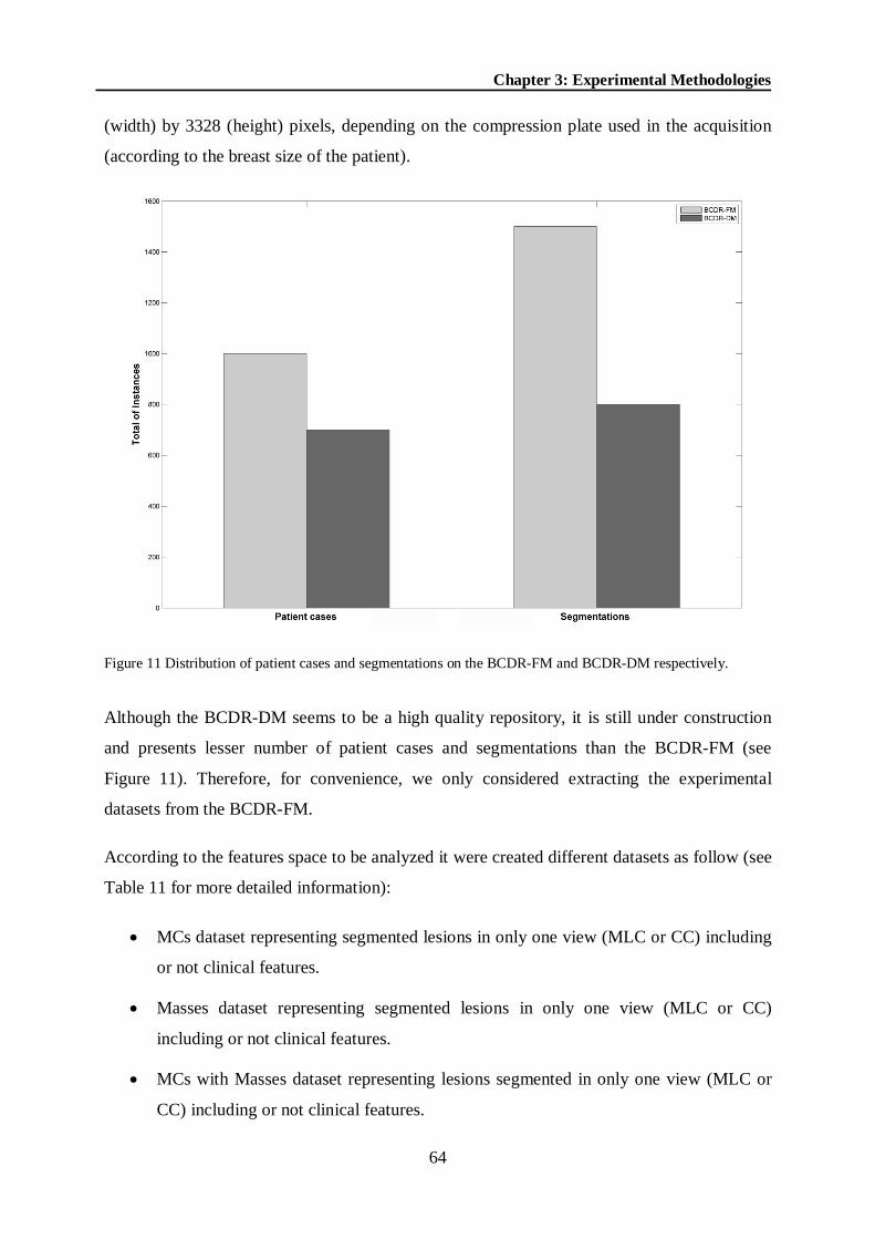
Chapter 3: Experimental Methodologies
64
(width) by 3328 (height) pixels, depending on the compression plate used in the acquisition
(according to the breast size of the patient).
Figure 11 Distribution of patient cases and segmentations on the BCDR-FM and BCDR-DM respectively.
Although the BCDR-DM seems to be a high quality repository, it is still under construction
and presents lesser number of patient cases and segmentations than the BCDR-FM (see
Figure 11). Therefore, for convenience, we only considered extracting the experimental
datasets from the BCDR-FM.
According to the features space to be analyzed it were created different datasets as follow (see
Table 11 for more detailed information):
MCs dataset representing segmented lesions in only one view (MLC or CC) including
or not clinical features.
Masses dataset representing segmented lesions in only one view (MLC or CC)
including or not clinical features.
MCs with Masses dataset representing lesions segmented in only one view (MLC or
CC) including or not clinical features.

Chapter 3: Experimental Methodologies
65
MCs dataset representing segmented lesions in an ipsilateral image view (MLC and
CC), including or not clinical features.
Masses dataset representing segmented lesions in an ipsilateral image view (MLC and
CC), including or not clinical features.
MCs with Masses dataset representing lesions segmented in an ipsilateral image view
(MLC and CC), including or not clinical features.
MCs with Masses balanced dataset (same number of instances per class) formed from
the BCDR-F01 (biopsy-proven diagnostic dataset).
MCs with Masses unbalanced dataset (with more benign than malignant instances per
class) formed from the BCDR-F01 (biopsy-proven diagnostic dataset).
MCs with Masses unbalanced dataset (with more malignant than benign instances per
class) formed from the BCDR-F01 (biopsy-proven diagnostic dataset).
3.1.2. DDSM
The DDSM database is composed by 2620 patient cases divided into three categories: normal
cases (12 volumes), cancer cases (15 volumes) and benign cases (14 volumes) [112]; each
case may have one or more associated Pathological Lesion (PL) segmentations, usually in
MLO and CC image views of the same breast. In addition to the PL segmentations and
density of the breast, the DDSM dataset also includes the subtlety of the lesion (an integer
number ranging between 1 and 5). Regarding the observations of the radiologists about the
lesions, DDSM stores if there are masses or calcifications and characterizes the shape and
margins of masses as well as the type and distribution of calcifications using keywords of the
BI-RADS glossary.
Due to the substantial volume of information, we considered only 582 segmentations
representing two volumes of cancer (vol. 1 and 2) and benign (vol. 1 and 5) cases. These
volumes correspond to the scanner LUMISYS, which provides the highest resolution in the
database (50 microns). The produced images have an average size of 3,118 (width) by 5,001
(height) pixels and 3,600 grey levels in LJPG format. For better suitability, the images used in
this thesis were obtained from the IRMA project where the original LJPEG images of DDSM
were converted to 16 bits PNG format [115, 116].
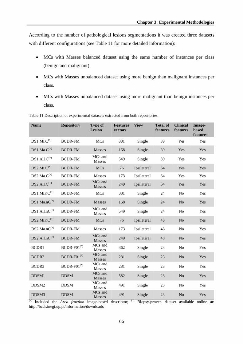
Chapter 3: Experimental Methodologies
66
According to the number of pathological lesions segmentations it was created three datasets
with different configurations (see Table 11 for more detailed information):
MCs with Masses balanced dataset using the same number of instances per class
(benign and malignant).
MCs with Masses unbalanced dataset using more benign than malignant instances per
class.
MCs with Masses unbalanced dataset using more malignant than benign instances per
class.
Table 11 Description of experimental datasets extracted from both repositories.
Name Repository Type of Lesion
Features vectors
View Total of features
Clinical features
Image-based features
DS1.Mi.C(+) BCDR-FM MCs 381 Single 39 Yes Yes
DS1.Ma.C(+) BCDR-FM Masses 168 Single 39 Yes Yes
DS1.All.C(+) BCDR-FM MCs and Masses 549 Single 39 Yes Yes
DS2.Mi.C(+) BCDR-FM MCs 76 Ipsilateral 64 Yes Yes
DS2.Ma.C(+) BCDR-FM Masses 173 Ipsilateral 64 Yes Yes
DS2.All.C(+) BCDR-FM MCs and Masses 249 Ipsilateral 64 Yes Yes
DS1.Mi.nC(+) BCDR-FM MCs 381 Single 24 No Yes
DS1.Ma.nC(+) BCDR-FM Masses 168 Single 24 No Yes
DS1.All.nC(+) BCDR-FM MCs and Masses 549 Single 24 No Yes
DS2.Mi.nC(+) BCDR-FM MCs 76 Ipsilateral 48 No Yes
DS2.Ma.nC(+) BCDR-FM Masses 173 Ipsilateral 48 No Yes
DS2.All.nC(+) BCDR-FM MCs and Masses 249 Ipsilateral 48 No Yes
BCDR1 BCDR-F01(*) MCs and Masses 362 Single 23 No Yes
BCDR2 BCDR-F01(*) MCs and Masses 281 Single 23 No Yes
BCDR3 BCDR-F01(*) MCs and Masses 281 Single 23 No Yes
DDSM1 DDSM MCs and Masses 582 Single 23 No Yes
DDSM2 DDSM MCs and Masses 491 Single 23 No Yes
DDSM3 DDSM MCs and Masses 491 Single 23 No Yes
(+) Included the Area fraction image-based descriptor; (*) Biopsy-proven dataset available online at: http://bcdr.inegi.up.pt/information/downloads
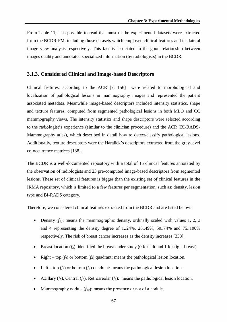
Chapter 3: Experimental Methodologies
67
From Table 11, it is possible to read that most of the experimental datasets were extracted
from the BCDR-FM, including those datasets which employed clinical features and ipsilateral
image view analysis respectively. This fact is associated to the good relationship between
images quality and annotated specialized information (by radiologists) in the BCDR.
3.1.3. Considered Clinical and Image-based Descriptors
Clinical features, according to the ACR [7, 156] were related to morphological and
localization of pathological lesions in mammography images and represented the patient
associated metadata. Meanwhile image-based descriptors included intensity statistics, shape
and texture features, computed from segmented pathological lesions in both MLO and CC
mammography views. The intensity statistics and shape descriptors were selected according
to the radiologist’s experience (similar to the clinician procedure) and the ACR (BI-RADS-
Mammography atlas), which described in detail how to detect/classify pathological lesions.
Additionally, texture descriptors were the Haralick’s descriptors extracted from the grey-level
co-occurrence matrices [138].
The BCDR is a well-documented repository with a total of 15 clinical features annotated by
the observation of radiologists and 23 pre-computed image-based descriptors from segmented
lesions. These set of clinical features is bigger than the existing set of clinical features in the
IRMA repository, which is limited to a few features per segmentation, such as: density, lesion
type and BI-RADS category.
Therefore, we considered clinical features extracted from the BCDR and are listed below:
Density (f1): means the mammographic density, ordinally scaled with values 1, 2, 3
and 4 representing the density degree of 1..24%, 25..49%, 50..74% and 75..100%
respectively. The risk of breast cancer increases as the density increases [238].
Breast location (f2): identified the breast under study (0 for left and 1 for right breast).
Right – top (f3) or bottom (f4) quadrant: means the pathological lesion location.
Left – top (f5) or bottom (f6) quadrant: means the pathological lesion location.
Axillary (f7), Central (f8), Retroareolar (f9): means the pathological lesion location.
Mammography nodule (f10): means the presence or not of a nodule.

Chapter 3: Experimental Methodologies
68
Mammography calcification (f11): means the presence or not of a calcification.
Mammography microcalcification (f12): means the presence or not of a
microcalcifications.
Mammography axillary adenopathy (f13): means the presence or not of an axillary
adenopathy.
Mammography architectural distortion (f14): means the presence or not of an
architectural distortion.
Mammography stroma distortion (f15): means the presence or not of architectural
distortion.
Besides, image-based descriptors in the BCDR were computed from the lesions contour,
which is stored in Cartesian coordinates. However, in the IRMA database the lesions contour
was stored using a chain-code technique making more difficult the computation of any
descriptors. Thus, it was necessary implementing a MATLAB (version R2011a) interface to
compute the same image-based descriptors (see Figure 12).
Figure 12 A screenshot of the developed MATLAB interface for the automatic computation of image-based descriptors. An example using the patient number A_1054_1 of the IRMA repository.

Chapter 3: Experimental Methodologies
69
The mathematical formulations of implemented image-based descriptors are presented below:
Skewness:
3
1
2
1
3
16
)(1
)(1
n
ii
n
ii
xxn
xxn
f (6)
with ix being the ith-value and x the sample mean.
kurtosis:
3
)(1
)(1
2
1
2
1
4
17
n
ii
n
ii
xxn
xxn
f (7)
with ix being the ith-value and x the sample mean.
Area fraction (f18): is the percentage of non-zero pixels in the image or selection.
Circularity:
219 4perimeter
areaf (8)
Perimeter:
)(20 Elengthf (9)
with OE being the edge pixels.
Elongation:
Mmf /21 (10)
with m being the minor axis and M the major axis of the ellipse that has the same
normalized second central moments as the region surrounded by the contour.

Chapter 3: Experimental Methodologies
70
Standard deviation:
n
ii xx
nf
1
222 )(
11 (11)
with ix being the grey level intensity of the ith pixel and x the mean of intensity.
Roughness:
areaperimenterf
*4)( 2
23 (12)
Minimum (f24) and Maximum (f25): The minimum and maximum intensity value in the
region surrounded by the contour.
Shape:
areaElongationperimeterf
*8*
26 (13)
X centroid:
227max(x)min(x)f
(14)
with x being the set of X coordinates of the object’s contour.
Entropy:
L
i
L
j
jipjipf1 1
28 ),(log),( (15)
with p(i,j) being the probability of pixels with grey-level i occur together to pixels
with grey-level j.
X center mass (f29) and Y center mass (f30): Normalized X and Y coordinates of the
center of mass of O.

Chapter 3: Experimental Methodologies
71
Energy:
L
i
L
j
jipf1 1
231 ),( (16)
with L being the number of grey-levels, and p being the grey-level co-occurrence
matrix and, thus, p(i,j) is the probability of pixels with grey-level i occur together to
pixels with grey-level j.
Median:
evenisXlengthif
nXnXMED
oddisXlengthifnMED
f
)(,2
)12
()2
(
)(,2
1
32 (17)
with X being the set of intensities.
Contrast:
i j
jipjif ),()( 233 (18)
with p(i,j) being the probability of pixels with grey-level i occur together to pixels
with grey-level j.
Correlation:
yx
i jyxjipij
f
),()(
34 (19)
with xyx ,, and y being the means and standard deviations of the marginal
distribution associated with p(i,j).

Chapter 3: Experimental Methodologies
72
Mean:
n
iix
nf
135
1 (20)
with n being the number of pixels inside the region delimited by the contour and xi
being the grey level intensity of the ith pixel inside the contour.
Homogeneity:
i j
jipji
f ),()(1
1236 (21)
with p(i,j) being the probability of pixels with grey-level i occur together to pixels
with grey-level j.
Area:
Of 37 (22)
with O being the set of pixels that belong to the segmented lesion.
Y centroid:
238max(Y)min(Y)f
(23)
with Y being the set of Y coordinates of the object’s contour.
Statistical mode (f39): Most frequent intensity value in a segmented ROI (lesion).

Chapter 3: Experimental Methodologies
73
3.2. Feature Selection
As it was mentioned in previous chapter, there are many potential benefits of features
selection, i.e. facilitating data visualization and data understanding, reducing the measurement
and storage requirements, reducing training and utilization times, defying the curse of
dimensionality to improve prediction performance [56, 60]. However, these advantages come
at a certain price, as the search for a subset of relevant features introduces an additional layer
of complexity in the modeling task; the one of finding an optimal subset of relevant features
[61, 62]. This is not practical in most situations because the number of possible subsets given
N features is 2N−1 (the empty set is excluded), which means NP-hard algorithms [56].
Therefore, in practical machine learning applications, usually a satisfactory instead of the
optimal feature subset is searched.
We considered the application of four traditional features selection methods and another one
developed from our own initial exploration made in this area (we named RMean). All
employed methods belong to the filter paradigm, because its execution is a one step process
without any data exploration (search) involved and are also independent of classifiers [239].
In addition, these methods use different evaluation function, which provides important
information about the nature of each feature (dependence with respect to the class) in the
features space. Typically, an evaluation function tries to measure the discriminating ability of
a feature or a subset of features to distinguish the different class labels. Thus, an optimal
subset chosen using one evaluation function may not be the same as that which uses another
evaluation function [240].
The selected methods were:
CHI2 discretization [96]: This method consists on a justified heuristic for supervised
discretization. Numerical features are initially sorted by placing each observed value
into its own interval. Then the chi-square statistic is used to determine whether the
relative frequencies of the classes in adjacent intervals are similar enough to justify
merging. The extent of the merging process is controlled by an automatically set chi-
square threshold. The threshold is determined through attempting to maintain the
fidelity of the original data.

Chapter 3: Experimental Methodologies
74
IG method: The IG measurement normalized with the symmetrical uncertainty
coefficient [98] is a symmetrical measure in which the amount of information gained
about Y after observing X is equal to the amount of information gained about X after
observing Y (a measure of feature-feature intercorrelation). This model is used to
estimate the value of an attribute Y for a novel sample (drawn from the same
distribution as the training data) and compensates for information gain bias toward
attributes with more values.
1Rule [241]: This method estimates the predictive accuracy of individual features
building rules based on a single feature (can be thought of as single level decision
trees). As we used training and test datasets, it is possible to calculate a classification
accuracy for each rule and hence each feature. Then, from classification scores, a
ranked list of features is obtained. Experiments with choosing a selected number of the
highest ranked features and using them with common machine learning algorithms
showed that, on average, the top three or more features are as accurate as using the
original set. This approach is unusual due to the fact that no search is conducted.
Relief [174]: This method uses instance based learning to assign a relevance weight to
each feature. Each feature weight reflects its ability to distinguish among the class
values. The feature weight is updated according to how well its values distinguish the
sampled instance from its nearest hit (instance of the same class) and nearest miss
(instance of opposite class). The feature will receive a high weight if it differentiates
between instances from different classes and has the same value for instances of the
same class. For nominal features it is defined as either 1 (the values are different) or 0
(the values are the same), while for numeric features the difference is the actual
difference normalized to the interval [0..1].
3.3. Exploring Classifiers
In this thesis, the problem of breast cancer classification is modeled as a two-class (binary)
classification problem with two discrete values: benign and malignant respectively. Therefore,
the discrimination between samples of two classes may be formulated as a supervised learning
problem, which is defined as the prediction of the value of a function for any valid input after
training a MLC using examples of input and target output pairs [125].

Chapter 3: Experimental Methodologies
75
Several MLCs have been used in Breast Cancer CADx systems. We used five of the most
employed: FFBP neural network, SVM, LDA, kNN, NB and DT J48, which are implemented
and available on Weka version 3.6 [242]. For all MLC with the exception of the NB (which
are parameterless), 10-fold cross validation method [243] was applied on the training set for
optimizing the classifiers’ parameters. A brief description and parameters configuration of
employed MLCs is given here:
The FFBP neural network is a particular model of ANN, which provides a nonlinear
mapping between its input and output according to the back-propagation error learning
algorithm. This model has demonstrated to be capable of approximating an arbitrarily
complex mapping within a finite support using only a sufficient number of neurons in
few hidden layers [244]. We used this classifier with the following parameters:
neurons on hidden layers were determined according to the equation (attributes +
number of classes)/2; one output layer associated with the binary classification
(benign or malignant); the sigmoid function was used as transfer function for all layers
and the number of iterations (epochs) were optimized in the range of 100 to 1000
epochs (with an interval increment of 100 units).
The SVM classifier, which is based on the definition of an optimal hyperplane, which
linearly separates the training data. In comparison with other classification methods, a
SVM aims to minimize the empirical risk and maximize the distances (geometric
margin) of the data points from the corresponding linear decision boundary [77, 244].
The SVM classifier was used with the following settings: the regularization parameter
C (cost) was optimized in the range of 10-3 to 103 and the kernel type was based on a
linear function, which provided better results respect to others kernel such as: radial
basis, polynomial and sigmoid function (from our experimental experience).
LDA is a traditional method for classification [213]. The basic idea is to try to find an
optimal projection (decision boundaries optimized by the error criterion), which can
maximize the distances between samples from different classes and minimize the
distances between samples from the same class. We used LDA for binary
classification, thus, observations were classified by the following linear function:
21)(g i icxWx iT
i (24)

Chapter 3: Experimental Methodologies
76
where TiW is the transpose of a coefficient vector, x is a feature vector and ci is a
constant as the threshold. The values of TiW and ci are determined through the analysis
of a training set. Once these values are determined, they can be used to classify the
new observations (smallest )(g i x is preferred).
The kNN classifier is a nonparametric technique called a ‘lazy learning’ because little
effort goes into building the classifier and most of the work is performed at the time of
classification. The kNN assigns a test sample to the class of the majority of its k-
neighbors; that is, assuming that the number of voting neighbors is k=k1+k2+k3 (where
ki is the number of samples from class i in the k-sample neighborhood of the test
sample, usually computed using the Euclidean distance), the test sample is assigned to
class m if 3,2,1),max( ikk im [210]. We used the kNN classifier including the
estimation of an optimal value k for the size of the neighborhood varying from 1 to 20,
and the contribution of each neighbor was always weighted by the distance to the
instance being classified.
The NB classifier is based on probabilistic models with strong (Naive) independence
assumptions, which assumes that a class variable depends of the set of input features
[245]. This classifier can be trained based on the relative frequencies shown in the
training set to get an estimation of the class priors and feature probability distributions.
For a test sample, the decision rule will be picking the most probable hypothesis,
which is known as the maximum a posteriori decision rule using the above model.
The DTJ48 classifier. This model is a standard tree, which has the useful characteristic
of generating tree-based models that human experts can easily interpret [244], where
non-terminal nodes represent tests on one or more attributes and terminal nodes reflect
decision outcomes. The Classification algorithm in DTJ48 is inductively learned
constructing a model from the pre-classified dataset. Each data item is defined by
values of the attributes. Due to this, the classification may be viewed as a mapping
from a set of features to a particular class. The DTJ48 classifier was used with a
confidence factor varying from 10-2 to 102 (with an interval increment of 0.1 units) and
2 leaf per node (to guarantee the binary model).

Chapter 3: Experimental Methodologies
77
3.4. The RMean Method
RMean is an ensemble method based on the mean criteria and it is supported on the filter
paradigm [4, 246]. It considers that an optimal subset of features is always relative to a certain
evaluation function, thus, the use of different evaluation function provides important
information about the nature of each feature (dependence with respect to the class) in the
features space [240].
The RMean method used as input four feature selection methods with different evaluation
function from the filter paradigm: CHI2 discretization [96] based on the chi-square statistic
function, IG [98] based on the information measure, 1Rule [241] based on rules as evaluation
functions and Relief [174] based on the distance measure. These four methods were applied
on the experimental datasets under analysis to produce four different ranking of features (one
by each applied feature selection method). Then the mean position of each feature along the
four features ranking was computed. Finally, a new ranking was created using the mean
position of features as indexing criterion. Table 12 shows a pseudo-code describing the
developed RMean method.
Table 12 The RMean method
RMean input:
),...,,( 21 NFFFD // A training dataset with N features output:
meanR // Final ranking of features 1. Begin 2. ),2(2 DCHIevalRchi // Application of CHI2 discretization method to
the D dataset. 3. ),( DIGevalRIG // Application of IG method to the D dataset. 4. ),1(1 DRuleevalR Rule // Application of 1Rule method to the D dataset.
5. ),( DreliefevalRrelief // Application of Relief method to the D dataset.
6. 4/)( 12 reliefRuleIGchimean RRRRR // Averaging the features position throughout resultant rankings from steps 2,3,4 and 5.
7. )'', ( ascendantRsortingR meanmean // Sorting in ascendant way the resultant ranking from the step 6.
8. End
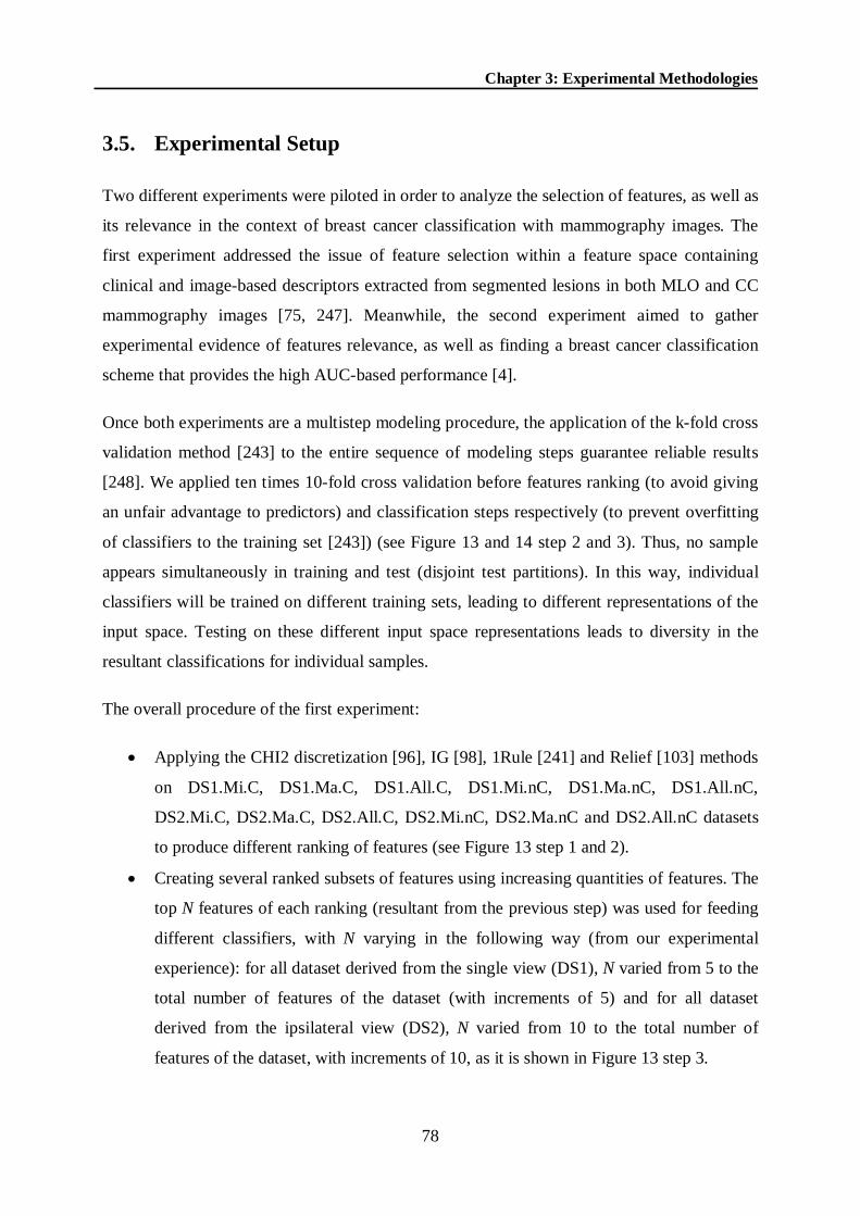
Chapter 3: Experimental Methodologies
78
3.5. Experimental Setup
Two different experiments were piloted in order to analyze the selection of features, as well as
its relevance in the context of breast cancer classification with mammography images. The
first experiment addressed the issue of feature selection within a feature space containing
clinical and image-based descriptors extracted from segmented lesions in both MLO and CC
mammography images [75, 247]. Meanwhile, the second experiment aimed to gather
experimental evidence of features relevance, as well as finding a breast cancer classification
scheme that provides the high AUC-based performance [4].
Once both experiments are a multistep modeling procedure, the application of the k-fold cross
validation method [243] to the entire sequence of modeling steps guarantee reliable results
[248]. We applied ten times 10-fold cross validation before features ranking (to avoid giving
an unfair advantage to predictors) and classification steps respectively (to prevent overfitting
of classifiers to the training set [243]) (see Figure 13 and 14 step 2 and 3). Thus, no sample
appears simultaneously in training and test (disjoint test partitions). In this way, individual
classifiers will be trained on different training sets, leading to different representations of the
input space. Testing on these different input space representations leads to diversity in the
resultant classifications for individual samples.
The overall procedure of the first experiment:
Applying the CHI2 discretization [96], IG [98], 1Rule [241] and Relief [103] methods
on DS1.Mi.C, DS1.Ma.C, DS1.All.C, DS1.Mi.nC, DS1.Ma.nC, DS1.All.nC,
DS2.Mi.C, DS2.Ma.C, DS2.All.C, DS2.Mi.nC, DS2.Ma.nC and DS2.All.nC datasets
to produce different ranking of features (see Figure 13 step 1 and 2).
Creating several ranked subsets of features using increasing quantities of features. The
top N features of each ranking (resultant from the previous step) was used for feeding
different classifiers, with N varying in the following way (from our experimental
experience): for all dataset derived from the single view (DS1), N varied from 5 to the
total number of features of the dataset (with increments of 5) and for all dataset
derived from the ipsilateral view (DS2), N varied from 10 to the total number of
features of the dataset, with increments of 10, as it is shown in Figure 13 step 3.

Chapter 3: Experimental Methodologies
79
Classifying the generated ranked subsets of features using FFBP neural network [244],
SVM [77, 244], and DTJ48 [75] classifiers for a statistical comparative analysis of
AUC scores, all comparisons were using the Wilcoxon statistical test [249-251] (see
Figure 13 step 3).
Analyzing the relevance of features by the separation of all features ranking into four
ranking groups: Single and Multiview Ranking including Clinical features and, Single
and Multiview Ranking without including Clinical features. For each group, it was
computed the total of features to be analyzed by averaging the size of the features
subset in each winner scheme. Finally, the feature relevance was decided by averaging
its position throughout all features ranking within the group under analysis.
Figure 13 Flowchart of the first experiment; filled box represents the presence of clinical features.
The overall procedure of the second experiment:
Applying the CHI2 discretization [96], IG [98], 1Rule [241], Relief [103] and RMean
[4, 246] methods on DS2.Mi.C and DS2.Ma.C datasets to produce different ranking of
features (see Figure 14 step 1 and 2).
Creating several ranked subsets of features using increasing quantities of features. The
top N features of each ranking (resultant from the previous step) were used for feeding
different classifiers, with N varying from 10 to the total number of features of the
dataset, with increments of 10 (from our experimental experience) as it is shown in
Figure 14 step 3.

Chapter 3: Experimental Methodologies
80
Classifying the generated ranked subsets of features using FFBP neural network [244],
SVM [77, 244], LDA [213, 214], kNN [210] and NB [245] classifiers for a statistical
comparative analysis of AUC scores, all comparisons were using the Wilcoxon
statistical test [249-251] (see Figure 14 step 3).
Discovering features with higher importance for MCs and masses classification
throughout (1) the validation of selected features as the most appropriate ranked subset
of features for breast cancer classification and (2) the selection of features with higher
importance inside each dataset.
Figure 14 Flowchart of the second experiment; filled box means the developed RMean method.
3.6. Results and Discussions
In this section, the empirical evaluation and discussion of results will be presented according
to the experimental setup section: first and second experiment respectively.
3.6.1. First Experiment
In this experiment, a total of 300 ranked subsets of features containing clinical and image
based features were classified using FFBP neural network, SVM and DTJ48 classifiers in
order to gather experimental evidences of variable selection within a feature space containing
clinical and image-based descriptors extracted from segmented lesions in both MLO and CC
mammography images. The obtained results showed reliable performances in the

Chapter 3: Experimental Methodologies
81
classification of MCs, masses and both lesions together in the same dataset (see Figures 15,
16, 17, 18, 19 and 20).
Classification of Microcalcifications
Particular results for MCs classification illustrated that the best combination for DS1.Mi.C
dataset was formed by the DTJ48 classifier and the IG method with a total of 20 features (see
Figure 15 c). The reached AUC of 0.91 was significantly superior (p<0.05) to others
satisfactory results such as: the obtained by the FFBP neural network classifier and the CHI2
discretization method with 25 features, attaining an AUC value of 0.88 (see Figure 15 a, and
the SVM classifier with the CHI2 discretization method using a total of 20 features, achieving
an AUC value of 0.893 (see Figure 15 b). Table 13 shows the AUC-based statistical
comparison among these combinations.
Table 13 The AUC-based statistical comparison among the three best combinations on DS1.Mi.C dataset
Classification Model Number of Features 5 10 15 20 25 30 35 39 FFBP neural network / CHI2 discretization 0.805 0.86 0.795 0.863 0.888 0.845 0.835 0.835
SVM / CHI2 Discretization 0.807 0.843 0.873 0.893 0.87 0.845 0.855 0.83 DTJ48 / IG method 0.86 0.88 0.893 0.91(*) 0.888 0.898 0.878 0.87
(*) Statistically superior among all values at p<0.05; Bold value means the higher AUC score; Underlying value means the selected one scheme.
The most prominent results for the MCs dataset without the inclusion of clinical features
(DS1.Mi.nC) were obtained using the schemes formed by the CHI2 discretization method
with 5 features in conjunction with: the FFBP neural network and SVM classifiers, attaining
AUC value of 0.8344 and 0.8301 respectively (see Figure 15 d, and e).
Table 14 The AUC-based statistical comparison among the three best combinations on DS1.Mi.nC dataset
Classification Model Number of Features 5 10 15 20 24
FFBP neural network / CHI2 discretization 0.8344(+) 0.7822 0.7497 0.7792 0.7768
SVM / CHI2 Discretization 0.8301(+) 0.8156 0.7035 0.7807 0.7454 DTJ48 / CHI2 Discretization 0.8031 0.7506 0.7365 0.8207 0.7835
(+) No significant difference among them at p<0.05; Bold value means the higher AUC score; Underlying score means the selected one scheme.
From Table 14 it is possible to analyze that two classification schemes could be considered as
appropriate for MCs classification on datasets without including clinical features. According

Chapter 3: Experimental Methodologies
82
to the Wilcoxon statistical test [249, 250], they do not present significant difference in the
performances (p<0.05). However, it was selected as the best scheme the combination which
used the SVM classifier. Because it is a classification model less complex than the
combination using the FFBP neural network classifier.
Figure 15 The mean of AUC scores (on 100 runs) of different classification schemes on DS1.Mi.C (first row) and DS1.Mi.nC (second row) datasets.
For the MCs dataset using clinical features and image-based descriptors extracted from both
MLO and CC image view (DS2.Mi.C), the results highlighted three combinations with the
same performance (AUC value of 0.7604): the FFBP neural network classifier and the 1Rule
method using 30 features; the SVM classifier and the IG method with 50 features and the
DTJ48 classifier with the IG method using 50 features (see Figure 16 a, b, c).

Chapter 3: Experimental Methodologies
83
Figure 16 The mean of AUC scores (on 100 runs) of different classification schemes on DS2.Mi.C (first row) and DS2.Mi.nC (second row) datasets.
This result was statistically superior to the remaining schemes (see Table 15). However, it is
reasonable to consider the first combination (the FFBP neural network classifier and the
1Rule method with 30 features) as the most appropriate scheme for MCs classification in this
dataset, due to the fact of reaching this performance using a fewer number of features than the
other two combinations (50 features).
Table 15 The AUC-based statistical comparison among the three best combinations on DS2.Mi.C dataset
Classification Model Number of Features 10 20 30 40 50 60 64 FFBP neural network / 1Rule method 0.7083 0.75 0.7604(+) 0.7438 0.7417 0.6583 0.6688
SVM / IG method 0.6417 0.6833 0.6979 0.7458 0.7604(+) 0.7188 0.6688 DTJ48 / IG method 0.6583 0.6917 0.6979 0.7458 0.7604(+) 0.7188 0.6729
(+) No significant difference among them at p<0.05; Bold value means the higher AUC score; Underlying value means the selected one scheme.
Besides, the classification results on DS2.Mi.nC dataset underlined as the best combination,
the scheme formed by the FFBP neural network classifier and the 1Rule method using 10
features, attaining an AUC value of 0.754 (see Figure 16 d, e and f). In this dataset, only a few
classification schemes provided AUC values superior to 0.70 (low classification
performance). As it can read in Table 16, the best classification result statistically overcomes
the remaining classification schemes.

Chapter 3: Experimental Methodologies
84
Table 16 The AUC-based statistical comparison among the three best combinations on DS2.Mi.nC dataset
Classification Model Number of Features 10 20 30 40 48
FFBP neural network / 1Rule method 0.7542(*) 0.6167 0.6438 0.6792 0.6542
SVM / 1Rule method 0.65 0.7063 0.6729 0.6625 0.6542 DTJ48 / CHI2 Discretization 0.7208 0.7 0.6604 0.6104 0.6438
(*) Statistically superior among all values at p<0.05; Bold value means the higher AUC score; Underlying value means the selected one scheme.
Classification of Masses
Several classification results, when using clinical features on masses, were superior to an
AUC value of 0.80 in the DS1.Ma.C dataset, which are globally considered as acceptable
results (see Figure 17 a, b and c). The higher AUC score of 0.9539 belongs to the
classification scheme formed by the SVM classifier and the CHI2 discretization method using
25 features (see Figure 17 b). However, this result was not statistically superior (p<0.05) to
obtained results by the combinations of the FFBP neural network classifier and the CHI2
discretization method with 20 features (AUC value of 0.9496), and the combination of the
SVM classifier with the CHI2 discretization method using 20 features, which had also a good
performance result (AUC value of 0.9485). Therefore, both combinations using 20 features
could be considered as most appropriated classification schemes for masses classification in
the DS1.Ma.C dataset. In this case, it was preferred the selection of the scheme formed by the
SVM classifier and the CHI2 discretization method using 20 features, due to the fact of being
a less complex classification model. The table 17 shows the best classification schemes for
DS1.Ma.C dataset and the statistical comparison among all of them.

Chapter 3: Experimental Methodologies
85
Table 17 The AUC-based statistical comparison among the three best combinations on DS1.Ma.C dataset.
Classification Model Number of Features 5 10 15 20 25 30 35 39 FFBP neural network / CHI2 discretization 0.8673 0.9015 0.9175 0.9496(+) 0.9426 0.9301 0.9256 0.9259
SVM / CHI2 Discretization 0.8666 0.9027 0.9325 0.9485(+) 0.9539(+) 0.9305 0.9289 0.9383 DTJ48 / IG method 0.8005 0.8712 0.9102 0.9254 0.9195 0.9349 0.9377 0.9300
(+) No significant difference among them at p<0.05; Bold value means the higher AUC score; Underlying value means the selected one scheme.
The masses classifications performances in the dataset without including clinical features
(DS1.Ma.nC) resulted in worse AUC scores with respect to the dataset including clinical
features (see Figure 18). Only classification schemes using the CHI2 discretization and IG
methods provided an AUC value superior to 0.80. The higher result in the DS1.Ma.nC dataset
was obtained by the combination of the SVM classifier and the CHI2 discretization method
with 15 features, attaining an AUC value of 0.8672 (see Table 18).
Table 18 The AUC-based statistical comparison among the three best combinations on DS1.Ma.nC dataset.
Classification Model Number of Features 5 10 15 20 24
FFBP neural network / CHI2 discretization 0.8601 0.8658(+) 0.8585 0.8603 0.8487
SVM / CHI2 Discretization 0.8576 0.83 0.8672(+) 0.8589 0.8536 DTJ48 / CHI2 Discretization 0.8031 0.8096 0.845 0.8634(+) 0.86
(+) No significant difference among them at p<0.05; Bold value means the higher AUC score; Underlying value means the selected one scheme.
From Table 18, the higher AUC value obtained by the SVM classifier and the CHI2
discretization method did not overcome statistically others combinations such as: the FFBP
neural network and DTJ48 classifiers with the same CHI2 discretization method using 10 and
20 features respectively. In this case, it was preferred the combination which used the smaller
number of features as the most appropriate classification scheme for masses classification in
the DS1.Ma.nC dataset.

Chapter 3: Experimental Methodologies
86
Figure 17 The mean of AUC scores (on 100 runs) of different classification schemes on DS1.Ma.C (first row) and DS1.Ma.nC (second row) datasets.
The best performance using DS2.Ma.C dataset was reached by the SVM classifier and the
1Rule discretization method with 30 features, reaching an AUC value of 0.9649 (see Figure
18 b). This higher result was almost statistically superior to the remainder classification
scheme. Only one combination using the same classifier and feature selection method with 40
features provided not significantly difference between them (see Table 19). However, the
most appropriate classification scheme for masses classification using the DS2.Ma.C dataset
is the combination which used smaller number of features without affecting the classification
performance (see Table 19).
Table 19 The AUC-based statistical comparison among the three best combinations on DS2.Ma.C dataset.
Classification Model Number of Features 10 20 30 40 50 60 64 FFBP neural network / IG method 0.9495 0.9103 0.9325 0.9373 0.9398 0.9523 0.9307
SVM / 1Rule method 0.9213 0.94 0.9649(+) 0.9609(+) 0.9589 0.9595 0.9374 DTJ48 / IG method 0.8598 0.9136 0.9511 0.9502 0.946 0.9406 0.9374
(+) No significant difference among them at p<0.05; Bold value means the higher AUC score; Underlying value means the selected one scheme.

Chapter 3: Experimental Methodologies
87
On the other hand, the best classification score using the DS2.Ma.nC dataset was acquired by
the FFBP neural network classifier in aggregation to the IG method with 40 features,
attainment an AUC value of 0.8899 (see Figure 18 d). This classification result was the
highest AUC value using the DS2.Ma.nC dataset, but it was not significantly different to the
combination formed by the SVM classifier and the 1Rule method using 40 features, which
reached an AUC value of 0.8863 (see Table 20).
Table 20 The AUC-based statistical comparison among the three best combinations on DS2.Ma.nC dataset.
Classification Model Number of Features 10 20 30 40 48
FFBP neural network / IG method 0.8004 0.854 0.8794 0.8899(+) 0.8742
SVM / 1Rule method 0.8394 0.863 0.8655 0.8863(+) 0.8643 DTJ48 / IG method 0.7316 0.8041 0.8275 0.8719 0.8643
(+) No significant difference among them at p<0.05; Bold value means the higher AUC score; Underlying value means the selected one scheme.
From Table 20, there are two combinations that can be used as the most appropriate
classification schemes for masses classification using the DS2.Ma.nC dataset. In this case, the
computation time and the simplicity of the classification model were the key for selecting the
scheme formed by the SVM classifier and the 1Rule method with 40 features.
Figure 18 The mean of AUC scores (on 100 runs) of different classification schemes on DS2.Ma.C (first row) and DS2.Ma.nC (second row) datasets.

Chapter 3: Experimental Methodologies
88
Classification of All Lesions (Masses and Microcalcifications together)
The classification results on datasets containing both lesions point as the winner combination
the SVM classifier and the CHI2 discretization method with 30 features in the DS1.All.C
dataset, attaining an AUC value of 0.934 (see Figure 19 b). This result was almost the winner
(in terms of AUC value) when comparing to the rest of the classification results. Two other
combinations provided similar satisfactory classification performance: the FFBP neural
network and SVM classifiers in conjunction with the CHI2 discretization method using 35
features. However, as it can be observed from Table 21, these combinations reached the best
classification performance with more features (35 features). Therefore, the selected
combination with 30 features constituted the best classification scheme for DS1.All.C dataset.
Table 21 The AUC-based statistical comparison among the three best combinations on DS1.All.C dataset.
Classification Model Number of Features 5 10 15 20 25 30 35 39 FFBP neural network / IG method 0.9055 0.9109 0.9113 0.9164 0.9149 0.9227 0.9279(+) 0.9260
SVM / CHI2 Discretization 0.8562 0.8533 0.8957 0.8984 0.9122 0.934(+) 0.928(+) 0.9264 DTJ48 / CHI2 Discretization 0.8626 0.8768 0.9037 0.9226 0.92 0.9254 0.9270 0.9256
(+) No significant difference among them at p<0.05; Bold value means the higher AUC score; Underlying value means the selected one scheme.
The best classification result for the DS1.All.nC dataset was obtained by the combination of
the SVM classifier and the CHI2 discretization method with 20 features; attaining an AUC
score of 0.843 (see Figure 19 e). This result statistically surpasses the remaining classification
schemes (see Table 22). Therefore, it could be considered as the most appropriated
classification scheme for this dataset.

Chapter 3: Experimental Methodologies
89
Table 22 The AUC-based statistical comparison among the three best combinations on DS1.All.nC dataset.
Classification Model Number of Features 5 10 15 20 24
FFBP neural network / CHI2 discretization 0.7957 0.81 0.8209 0.831 0.821
SVM / CHI2 Discretization 0.7806 0.8149 0.8188 0.843(*) 0.8305 DTJ48 / CHI2 Discretization 0.7743 0.7969 0.8054 0.823 0.8173
(*) Statistically superior among all values at p<0.05; Bold value means the higher AUC score; Underlying value means the selected one scheme.
Figure 19 The mean of AUC scores (on 100 runs) of different classification schemes on DS1.All.C (first row) and DS1.All.nC (second row) datasets.
The higher classification result in the DS2.All.C dataset was obtained by the combination of
the SVM classifier and the 1Rule method with 30 features, stretching an AUC value of 0.8874
(see Figure 20 b). According to the statistical test, this result was not the best classification
scheme. Two others combinations using a smaller set of features demonstrated to be
statistically similar in terms of classification performance (see Table 23). Thus, the most
appropriated classification scheme in this dataset was the one formed by the SVM classifier
and the 1Rule method using 20 features (AUC value of 0.8812), which provided a less
complex classification model.

Chapter 3: Experimental Methodologies
90
Table 23 The AUC-based statistical comparison among the three best combinations on DS2.All.C dataset.
Classification Model Number of Features 10 20 30 40 50 60 64 FFBP neural network / IG method 0.844 0.8832(+) 0.8443 0.8631 0.8572 0.8581 0.8401
SVM / 1Rule method 0.8731 0.8812(+) 0.8878(+) 0.8739 0.8698 0.86 0.8526 DTJ48 / IG method 0.8423 0.8495 0.8594 0.8629 0.8591 0.8535 0.8526
(+) No significant difference among them at p<0.05; Bold value means the higher AUC score; Underlying value means the selected one scheme.
The best classification result in the DS2.All.nC dataset was obtained by the combination of
the SVM classifier and the CHI2 discretization method using a total of 40 features (see Figure
20 e). This classification scheme provided the highest AUC value (0.8409) among all
combinations and also was statistically superior to the remainder results. Therefore, this
combination constituted the most appropriated classification scheme in this dataset (see Table
24).
Figure 20 The mean of AUC scores (on 100 runs) of different classification schemes on DS2.All.C (first row) and DS2.All.nC (second row) datasets.

Chapter 3: Experimental Methodologies
91
Table 24 The AUC-based statistical comparison among the three best combinations on DS2.All.nC dataset.
Classification Model Number of Features 10 20 30 40 48
FFBP neural network / CHI2 discretization 0.7771 0.7555 0.7837 0.8204 0.7914
SVM / CHI2 discretization 0.741 0.7652 0.7969 0.8409(*) 0.8111 DTJ48 / IG method 0.6796 0.757 0.8084 0.8135 0.8168
(*) Statistically superior among all values at p<0.05; Bold value means the higher AUC score; Underlying value means the selected one scheme.
Feature Relevance Analysis
The results listed in the previous section clearly provide experimental evidence that optimal
classification performance depends upon the appropriate choice of a classifier together with a
ranked subset of features and, the combination of clinical with image-based features increase
the classification performance substantially for all cases. Therefore, it was our intention to
find out the most important features in the whole features space.
The relevance of features was determined by the separation of 48 ranking of features (one by
each employed feature selection method on every experimental dataset) into four ranking
groups: Single View Ranking including Clinical features (SVRC), Single View Ranking
without including Clinical features (SVRNC), Multi View Ranking including Clinical
features (MVRC) and Multi View Ranking without including Clinical features (MVRC). For
each group, the total of features to be analyzed was computed by averaging the size of
features subset in each winner scheme. Finally, the relevance of feature was decided by
averaging its position along all rankings within the group under analysis.
Relevance within SVRC and MVRC groups
The SVRC group is formed by the ranked features extracted from DS1.Mi.C, DS1.Ma.C and
DS1.All.C datasets respectively and the total of features to be analyzed is approximately 25.
Therefore, we considered only the top 25 features of each ranking for features relevance
analysis in this group. Figure 21 shows the distribution of the average position for each
selected feature.

Chapter 3: Experimental Methodologies
92
Figure 21 Distribution of the average position for each selected clinical (filled box) and image-based (white box) features within the SVRC group.
The top clinical and image-based feature within this group was the Mammography stroma
distortion (f15) and Circularity (f19) with average positions of 2.5 and 4 respectively (see
Figure 21, f15 and f19). Even with a slight difference between them, the Mammography stroma
distortion (f15) clinical feature was the most consistent. Also, the presence of other clinical
(43%) and image-based (57%) features such as: Mammography calcification (f11), Density
(f1), Mammography microcalcification (f12), Mammography architectural distortion (f14),
Mammography nodule (f10), Mammography axillary adenopathy (f13), Retroareolar (f9), Right
top quadrant (f3), breast location (f2), Roughness (f23), Shape (f26), Perimeter (f20), Area (f37),
Entropy (f28), Contrast (f33), Energy (f31), Y center mass (f30), Y centroid (f38), standard
deviation (f32), X center mass (f29) and Correlation (f34) contributed to the classification
performances.
On the other hand, the MVRC group contains the ranked features extracted from DS2.Mi.C,
DS2.Ma.C and DS2.All.C datasets respectively and the total of features to be analyzes is 27.
Therefore, only 27 features were considered for relevance analysis. Similar to SVRC group,
the relevance analysis in this group highlighted as the top clinical and image-based features,
the Mammography stroma distortion (f15) and Circularity (f19) features with average positions

Chapter 3: Experimental Methodologies
93
of 2 and 4 respectively (see Figure 22). The f15 feature like in SVRC group appears as the
most consistent feature inside the group. The rest of clinical and image-based features
selected in this group were: Roughness (f23 and f23*), Perimeter (f20* and f20), Circularity (f19*),
Entropy (f28), Mammography calcification (f11), Area (f37* and f37), Density (f1), Y center
mass (f30 and f30*), Contrast (f33* and f33), Y centroid (f38 and f38*), Standard deviation (f22),
Energy (f31 and f31*), Shape (f26 and f26*), Mammography microcalcification (f12),
Mammography axillary adenopathy (f13), Elongation (f21) and Mammography nodule (f10). In
contrast with the SVRC group, the best classification performances and the equilibrium of
features representation (22% for clinical against to a 78% for image-based) in this group were
considered lower. These particular differences could be associated to the double presence of
image-based features (see Figure 22, features with asterisk) in the features vectors.
Figure 22 Distribution of the average position for each selected clinical (filled box) and image-based (white box) features within the MVRC group. Features with asterisk (*) represent a computed feature in the collateral view (MLO and CC).

Chapter 3: Experimental Methodologies
94
Relevance within SVRNC and MVRNC groups
The SVRNC group is formed by the ranked features extracted from DS1.Mi.nC, DS1.Ma.nC
and DS1.All.nC datasets respectively and the total of features to be analyzed is approximately
12. Therefore, only the top 12 features were considered for feature relevance analysis in this
group. Figure 23 shows the distribution of the average position for each selected feature.
Figure 23 Distribution of the average position for each selected image-based features within the SVRNC group.
The Perimeter (f20) feature (see Figure 23) was ranked as the top image-based feature within
the group, only two feature selection methods (1Rule and Relief) does not considered it as the
best feature, although it was ranked on the top 5. Also, the presence of other image-based
features such as: Entropy (f28), Area (f37), Standard deviation (f22), Energy (f31), Correlation
(f34), Roughness (f23), Circularity (f19), Minimum (f24), Kurtosis (f17), Elongation (f21) and
Skewness (f16) contributed to the classification performances.
The MVRNC group was created by the set of ranked features generated from DS2.Mi.nC,
DS2.Ma.nC and DS2.All.nC datasets respectively and the total of features to be analyzed in
this group is 30. The relevance analysis highlighted the Circularity (f19) as the best feature in
this group, with an average position of 2. The remaining contributions were provided by
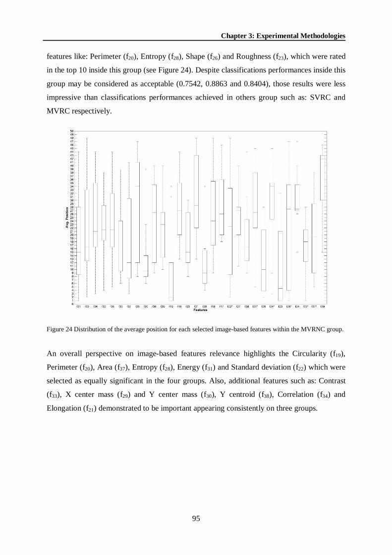
Chapter 3: Experimental Methodologies
95
features like: Perimeter (f20), Entropy (f28), Shape (f26) and Roughness (f23), which were rated
in the top 10 inside this group (see Figure 24). Despite classifications performances inside this
group may be considered as acceptable (0.7542, 0.8863 and 0.8404), those results were less
impressive than classifications performances achieved in others group such as: SVRC and
MVRC respectively.
Figure 24 Distribution of the average position for each selected image-based features within the MVRNC group.
An overall perspective on image-based features relevance highlights the Circularity (f19),
Perimeter (f20), Area (f37), Entropy (f28), Energy (f31) and Standard deviation (f22) which were
selected as equally significant in the four groups. Also, additional features such as: Contrast
(f33), X center mass (f29) and Y center mass (f30), Y centroid (f38), Correlation (f34) and
Elongation (f21) demonstrated to be important appearing consistently on three groups.
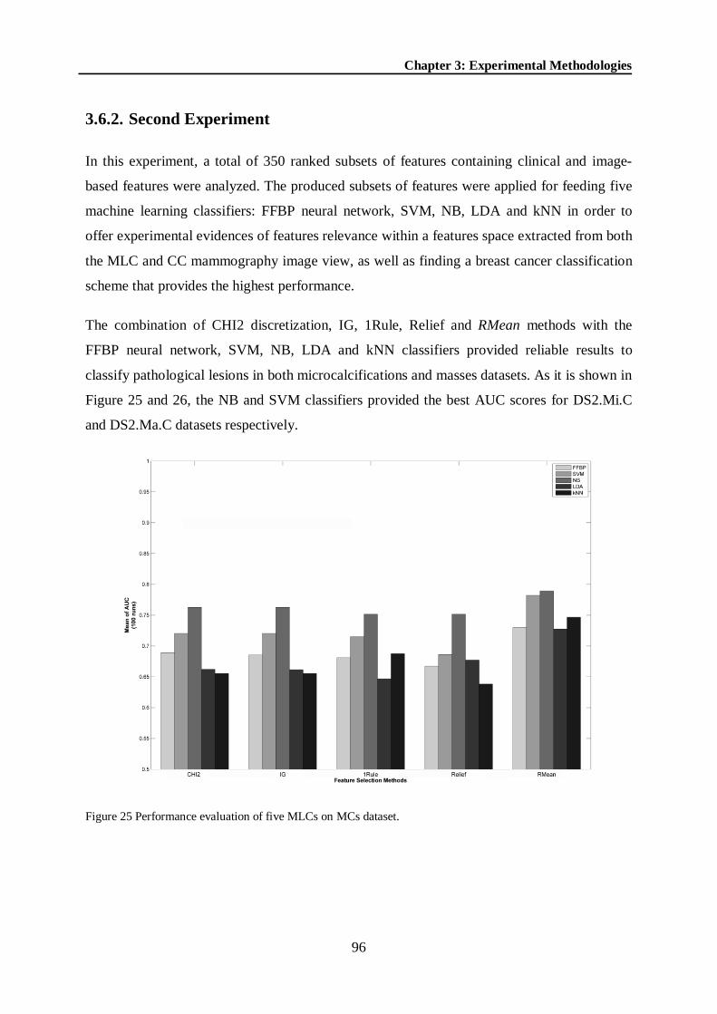
Chapter 3: Experimental Methodologies
96
3.6.2. Second Experiment
In this experiment, a total of 350 ranked subsets of features containing clinical and image-
based features were analyzed. The produced subsets of features were applied for feeding five
machine learning classifiers: FFBP neural network, SVM, NB, LDA and kNN in order to
offer experimental evidences of features relevance within a features space extracted from both
the MLC and CC mammography image view, as well as finding a breast cancer classification
scheme that provides the highest performance.
The combination of CHI2 discretization, IG, 1Rule, Relief and RMean methods with the
FFBP neural network, SVM, NB, LDA and kNN classifiers provided reliable results to
classify pathological lesions in both microcalcifications and masses datasets. As it is shown in
Figure 25 and 26, the NB and SVM classifiers provided the best AUC scores for DS2.Mi.C
and DS2.Ma.C datasets respectively.
Figure 25 Performance evaluation of five MLCs on MCs dataset.

Chapter 3: Experimental Methodologies
97
Figure 26 Performance evaluation of five MLCs on masses dataset.
Performance Evaluation
Classification results for MCs datasets illustrated that all machine learning classifiers
provided the best AUC score when using the RMean method. The higher AUC score was
obtained by the combination of the NB classifier and the RMean method with a total of 20
features, achieving an AUC score of 0.7893 with standard deviation of 0.16. Table 25 shows
the best classification performance on DS2.Mi.C dataset and the number of features employed
by each combination.
Table 25 The best classification performance based on AUC scores for the DS2.Mi.C dataset.
Pairs (FSM/MLC) CHI2 IG 1Rule Relief RMean
AUC NF AUC NF AUC NF AUC NF AUC NF
FFBP neural network 0.6890 30 0.6856 30 0.6810 30 0.6673 60 0.7298 10
SVM 0.7204 20 0.7204 20 0.7152 30 0.6860 60 0.7823 20
NB 0.7628 60 0.7628 60 0.7516 60 0.7516 60 0.7893 20
LDA 0.6621 10 0.6617 10 0.6469 10 0.6773 10 0.7275 10
kNN 0.6554 50 0.6554 50 0.6875 20 0.6383 20 0.7467 10 NF - means the number of features employed by each subset of features
From Table 25, it is possible to observe that RMean method increased the classification
performance based on AUC scores for all schemes (p<0.05). The same trend of results was

Chapter 3: Experimental Methodologies
98
not achieved with other schemes such as: the kNN classifier in conjunction with the CHI2
discretization, IG and Relief methods, which presented the worst AUC scores (0.6554, 0.6554
and 0.6383 respectively). Also, it is interesting to consider that these important results were
obtained with no more than 20 features.
According to obtained AUC scores, the best classification scheme was formed by the NB
classifier and the RMean method with 20 features (AUC score of 0.7893), which represented
an AUC numerical difference of: 0.0595, 0.007, 0.0618 and 0.0426 respect to the FFBP
neural network, SVM, LDA and kNN classifiers respectively. However, the statistical
comparison revealed there is a significant difference in most cases (p<0.05); only the scheme
formed by the SVM classifier and the RMean method using 20 features provided no
significant difference on AUC performances. Therefore, it is possible to consider both
combinations as appropriate MCs classification schemes (see Table 26).
Table 26 The statistical comparison based on the Wilcoxon Statistical Test for the DS2.Mi.C dataset.
Dataset Best scheme AUC Other winner scheme AUC Wilcoxon
(α= 0.05) Mean SD Mean SD
DS2.Mi.C NB+RMean+20F 0.7893 0.16
FFBP+RMean+10F 0.7298 0.18 p<0.01
SVM+RMean+20F 0.7823 0.17 p=0.8109
LDA+RMean+10F 0.7275 0.18 p<0.01
kNN+RMean+10F 0.7467 0.16 p<0.01 SD - Standard Deviation; F - Features.
In the case of masses classification, almost all machine learning classifiers provided the best
AUC score when using the RMean method, only the LDA classifier reached a higher AUC
score using another features selection method (see Table 30). The most important AUC score
was obtained by the combination of the SVM classifier and the RMean method with a total of
30 features, for an AUC score of 0.9549 with standard deviation of 0.05. Table 27 shows the
best classification performance on DS2.Ma.C dataset and the number of features employed by
each combination.

Chapter 3: Experimental Methodologies
99
Table 27 The best classification performance based on AUC scores for the DS2.Ma.C dataset.
Pairs (FSM/MLC) CHI2 IG 1Rule Relief RMean
AUC NF AUC NF AUC NF AUC NF AUC NF
FFBP neural network 0.9326 20 0.9307 60 0.9274 60 0.9324 50 0.9440 10
SVM 0.9522 50 0.9522 50 0.9483 40 0.9494 50 0.9549 30
NB 0.8747 10 0.8754 10 0.9011 30 0.9170 10 0.9267 10
LDA 0.9128 40 0.9128 40 0.9185 30 0.9122 20 0.9150 40
kNN 0.8226 20 0.8261 20 0.7827 20 0.7985 10 0.8279 30
NF- Number of Features
From Table 27, it is possible to perceive that the RMean method increased the classification
performance based on AUC scores for most schemes (p<0.05), which is globally considered
as good result. In contrast to the MCs classification, the number of selected features by each
scheme was superior on masses classification. Only two combinations reached high AUC
scores with the minimum number of features.
The best result based on AUC scores belongs to the scheme formed by the SVM classifier and
the RMean method with 30 features (AUC score of 0.9549), which represents an AUC
numerical difference of: 0.0109, 0.0282, 0.0364 and 0.127 with respect to the FFBP neural
network, NB, LDA and kNN classifiers respectively. According to the Wilcoxon statistical
test [249, 250] most of these numerical differences were statistically significant (p<0.05),
only one scheme presented no significant AUC difference (see Table 28). Therefore, both
combinations were considered as appropriate masses classification schemes. Table 28 shows
results of the statistical comparison between the best classification scheme and others winner
schemes.
Table 28 The statistical comparison based on the Wilcoxon Statistical Test for the DS2.Ma.C dataset.
Dataset Best scheme AUC Other winner scheme AUC Wilcoxon
(α= 0.05) Mean SD Mean SD
DS2.Ma.C SVM+RMean+30F 0.9549 0.05
FFBP+RMean+10F 0.9440 0.05 p=0.1256
NB+RMean+10F 0.9267 0.06 p<0.01
LDA+1Rule+30F 0.9185 0.07 p<0.01
kNN+RMean+30F 0.8279 0.09 p<0.01 SD - Standard Deviation; F- Features
Classification process on DS2.Mi.C and DS2.Ma.C datasets highlighted two winner schemes
for MCs and masses datasets respectively, in which the RMean method provided ranked
subsets of features with higher discriminant potential.

Chapter 3: Experimental Methodologies
100
Features Relevance Analysis
The results listed in Table 26 and 28 provided statistical evidences on selecting the most
appropriate classification scheme for MCs and masses datasets. From these results, two
combinations resulted as the best classification performances per dataset. Thus, the features
relevance analysis was conducted using these winner schemes and the following procedure:
(1) corroborating of selected features in the best classification scheme as the most appropriate
features subset for pathological lesions classification, and (2) determining features with higher
importance inside each dataset.
Features Subset Validation
The validation of selected features subsets and its impact in the classification performance
was based in the non-parametric Wilcoxon statistical test [249, 250] as the principal metric. In
this process we compared AUC performances between the best scheme and the same
combination using fewer features, and the key issue is to know how many features subsets
could be reduced without affecting the classification performance. Table 29 shows the
statistical results after applying the process of features subset validation.
Table 29 Results of the feature subset validation process.
Dataset Best scheme AUC Same scheme with
fewer features
AUC Wilcoxon
(α= 0.05) Mean SD Mean SD
DS2.Mi.C (1) NB+RMean+20F 0.7893 0.16 NB+RMean+10F 0.7395 0.20 p<0.01
(2) SVM+RMean+20F 0.7823 0.17 SVM+RMean+10F 0.7775 0.17 p=0.8109
DS2.Ma.C (3) SVM+RMean+30F 0.9549 0.05 SVM+RMean+10F 0.9271 0.06 p<0.01
(4) FFBP+RMean+10F 0.9440 0.05 N/A N/A N/A N/A SD- Standard Deviation; F- Features; N/A – Not Applicable
After completing the comparison, for MCs dataset (DS2.Mi.C) only one scheme provided
clear evidence of features subset reduction. From Table 29 it can be observed there is no
significant difference with respect to the obtained AUC scores between one of the most
appropriate schemes (scheme 2) and the same scheme using a more compact features subset.
Therefore, it was possible to reduce the features subset from 20 to 10 features without
affecting the consistency of the classification performance.
For the masses dataset (DS2.Ma.C), it was impossible the features subset reduction on one of
the most appropriate schemes (see Table 29 scheme 3) because there is statistical evidence on

Chapter 3: Experimental Methodologies
101
classification performance degradation. However, the scheme formed by the FFBP neural
network and the RMean method guaranteed the use of minimal quantity of features for
classifying masses. This means that selected features could be considered as the most relevant
features subset.
Features with Higher Importance
In the previous section, we showed how to determine if selected features subsets constitute the
most important extracted subset from the features space. From both DS2.Mi.C and DS2.Ma.C
datasets were extracted features subsets with a minimum number of features without affecting
the classification performance, which infers that selected features were relevant for MCs and
masses classification.
The most relevant features subset for MCs classification was composed by three clinical and
seven image-based features: Perimeter (f20), Standard deviation (f22 and f22*), Entropy (f28 and
f28*), Mammography stroma distortion (f15), Density (f1), Energy (f31 and f31*) and Right
bottom quadrant (f4). Clinical features like f15 and f4 were selected as relevant due to its great
capacity of discriminating between masses and MCs. The f15 feature means the presence of
architectural distortion that is a particular classification of masses. Meanwhile the f4 feature
means the location of the lesion, mostly used for MCs [7, 156]. As MCs are smaller and
brighter than masses, image-based features are very useful. For example, the f20 feature (top
ranked feature for MCs) will take smaller value than the f20 feature extracted from masses
lesions and constitutes a discriminant feature between masses and MCs. In general, image-
based features (intensity statistics, size, shape, etc.) are likely more employed for MCs
classification [7, 156].
The most relevant subset of features for masses classification was formed by four clinical and
six image-based features: Mammography stroma distortion (f15), Circularity (f19 and f19*),
Roughness (f23 and f23*), Shape (f26 and f26*), Mammography calcification (f11),
Mammography nodule (f10) and Density (f1). Clinical features like f15 and f10 were considered
strong features for masses classification because of the presence of architectural distortion
and/or nodules constitutes a particular masses classification. On the other hand, selected
image-based features were all associated to the shape and topology of masses. For example,
the f19 and f19* features (circularity features extracted from MLO and CC image view) are
measurements related to the mass shape classification [7, 156]. Also, the f23 and f23*

Chapter 3: Experimental Methodologies
102
(roughness features extracted from MLO and CC image view) are features associated to
lesions shape and topology. Generally when roughness value is near to zero means regular
contours, which is representative of benign masses, otherwise it is an indicative signal for
malignant masses or MCs (usually irregular contours is an indicative signal of malignant
lesions [7, 156]).
3.6.3. Global Discussion of Experiments
As it was designed in the experimental setup section, all results were separated in two
moments. The first one explored four traditional feature selection methods and three popular
machine learning classifiers using a massive features space, which included clinical and
image-based features extracted from single and ipsilateral pathological lesions segmentations
in mammography images. Meanwhile the second moment was aimed to find classification
schemes with less number of features and higher AUC-based performance for MCs and
masses classification.
Following obtained results in the first experiment, the Table 30 summarizes the best
classification schemes per dataset and the statistical comparison between AUC performances.
Table 30 The best classification scheme per dataset and the statistical comparison at p<0.05.
Dataset Classification Scheme AUC value NF
DS1.Mi.C DTJ48 classifier / IG method 0.91 20
DS1.Mi.nC SVM classifier / CHI2 discretization method 0.8301 5
DS2.Mi.C FFBP neural network classifier / 1Rule method 0.7604 30
DS2.Mi.nC FFBP neural network classifier / 1Rule method 0.7542 10
DS1.Ma.C SVM classifier / CHI2 discretization method 0.9485 20
DS1.Ma.nC FFBP neural network classifier / CHI2 discretization method 0.8658 10
DS2.Ma.C SVM classifier / 1Rule method 0.9649 30
DS2.Ma.nC SVM classifier / 1Rule method 0.8863 40
DS1.All.C SVM classifier / CHI2 discretization method 0.934 30
DS1.All.nC SVM classifier / CHI2 discretization method 0.843(+) 20
DS2.All.C SVM classifier / 1Rule method 0.8812 20
DS2.All.nC SVM classifier / CHI2 discretization method 0.8309(+) 40 NF- Number of Features; (+) No significant difference among them at p<0.05; Underlying value means the selected one scheme.
From Table 30, it is possible to observe that the best classification schemes for MCs lesions
were obtained on datasets with single image view (DS1.Mi.C and DS1.Mi.nC). These results

Chapter 3: Experimental Methodologies
103
were significantly superior to the obtained results by the classification schemes on ipsilateral
image view datasets (DS2.Mi.C and DS2.Mi.nC). The AUC value of 0.91 obtained by the
DTJ48 classifier and the IG method with 20 features in the DS1.Mi.C dataset represents a
significant performance increment of 0.15 (with p<0.005) respect to the best AUC score of
0.760 obtained by the FFBP classifier and the 1Rule method with 30 features on DS2.Mi.C
dataset. Meanwhile, the AUC value of 0.8301 obtained by the SVM classifier and the CHI2
discretization method using 5 features in the DS1.Mi.nC dataset constituted a significant
increment of 0.076 (with p<0.05) in the classification performance respect to the classification
result reached by the FFBP neural network classifier and the 1Rule method using 10 features
on DS2.Mi.nC dataset (0.7542).
In the case of masses classification (see Table 30), the best classification performances were
obtained on ipsilateral image view datasets (DS2.Ma.C and DS2.Ma.nC). These results were
significantly superior to the obtained results by the classification schemes on datasets with
single image view (DS1.Ma.C and DS1.Ma.nC). The AUC value of 0.9649 obtained by the
SVM classifier and the 1Rule method with 30 features in the DS2.Ma.C dataset represents a
slight significant performance increment of 0.16 (with p<0.005) respect to the best AUC score
of 0.9485 obtained by the SVM classifier and the CHI2 discretization method with 20 features
on DS1.Ma.C dataset. Meanwhile, the AUC value of 0.8863 obtained by the SVM classifier
and the 1Rule method using 40 features in the DS2.Ma.nC dataset constituted a significant
increment of 0.021 (with p<0.05) in the classification performance respect to the classification
result reached by the FFBP neural network classifier and the CHI2 discretization method
using 10 features on DS1.Ma.nC dataset (0.8658).
On the other hand, for all lesions together, the best classification schemes were obtained on
datasets using the single image view (DS1.All.C and DS1.All.nC). The AUC value of 0.934
obtained by the best classification scheme (SVM classifier and the CHI2 discretization with
30 features) in the DS1.All.C dataset represented a significant improvement of 0.053 in the
AUC value against to the obtained result by the best scheme in the DS2.All.C dataset (SVM
classifier and the 1Rule with 20 features), which stretched an AUC value of 0.8812. Also, the
best classification scheme (SVM classifier and the CHI2 discretization method with 20
features) in the DS1.All.nC dataset provided an AUC value of 0.843 against to a 0.8409
reached by the best classification scheme (SVM classifier and the CHI2 discretization method
with 40 features) in the DS2.All.nC dataset. These results were not significantly different
(p=0.089) in term of classification performance. However, the classification scheme using a

Chapter 3: Experimental Methodologies
104
fewer number of features constituted a less complex classification model and it was preferred
(see Table 30).
The statistical difference in AUC performances between single and ipsilateral image view
datasets could be explained by the fact of MCs lesions being smaller and brighter than masses
lesions [7]. Thus, image-based features extracted from intensity statistics and shapes of
segmented MCs in one image view could be considered sufficient for MCs classification. In
contrast, masses lesions tend to be obscured and confused with the surrounding tissues. As
they are very often characterized by its shape and margin [7], the use of more image-based
descriptors extracted from texture, shape and margin of segmented masses on both MLO and
CC image view could facilitate its classification.
In terms of features representation it was concluded that the inclusion of clinical features
always improved the classification performance for all classification schemes. The balance of
features participation between clinical and image-based descriptors was 43% (clinical) against
57% (image-based) for MCs classification and 22% (clinical) against 78% (image-based) for
masses classification. These results explained why the best masses classification schemes
were obtained using subsets of features extracted from segmented lesions in the ipsilateral
image view (image-based descriptors computed from MLO and CC image view).
Regarding the features selection methods and machine learning classifiers, it is possible to
observe that the best classification model was formed by the CHI2 discretization features
selection method and the SVM classifier; they consistently appeared as the most prominent
combination. Other combinations that performed well were: the 1Rule method and SVM
classifier; the CHI2 discretization method and FFBP neural network. Finally, all of these
combinations could be considered as appropriate classification schemes for breast cancer
classification.

Chapter 3: Experimental Methodologies
105
Despite the important results reported in the first experiment, it was detected a critical
limitation:
The mean of the number of employed features by the best classification schemes is
still elevated: for single image view datasets using clinical features was around 23.33
features (60%); for single image view datasets without using clinical features was
around 11.66 features (49%); for ipsilateral image view datasets with clinical features
was around 26.66 features (42%) and for ipsilateral image view datasets without
clinical features was around 30 features (63%).
Following this limitation, the second experiment provided experimental results of a new
developed feature selection method (RMean) using MCs and masses ipsilateral image view
datasets with clinical features.
The RMean method was able to provide ranked subsets of features with no more than 20
features, which increased statistically (p<0.05) the classification performance for all
classification schemes in the MCs dataset (see Table 25). The same trend of results was
obtained in the majority of classification schemes for the masses dataset. Only the LDA
classifier considered another feature selection method (1Rule) instead the developed RMean
method (see Table 27). However, as it is shown in Table 27 there is no significant difference
of performance between them.
According to the statistical results presented in the Table 30, it was possible reducing the
number of features employed by the best classification scheme on MCs and masses datasets.
Both classification schemes were condensed from 20 to 10 features without affecting the
classification performance. This means that the developed RMean method provides
competitive subsets of features with higher discriminant power.
Regarding performance of the RMean method, these results were expected since the RMean
method is based on the combination of four different feature evaluation functions, which
mean that an unfairly underrated feature by any feature selection method could have a chance
to be ranked as an important feature in the final ranking (output). However, the RMean is an
univariate filter feature selection method which presents two important drawbacks: (1) it is an
individual evaluator of features and it ignores the feature dependencies and, (2) it is dependent
of data normalization (since CHI2 and IG method are based on statistical test) and samples
sizes, which mean it is vulnerable to unbalanced training data.

Chapter 3: Experimental Methodologies
106
Concerning relevant features, the overlay analysis between the features subset selected in the
MVRC group of the first experiment (f15, f19, f23, f23*, f20*, f19*, f28, f20, f11, f37*, f37, f1, f30, f33*,
f38, f22, f30*, f31, f38*, f33, f26, f12, f26*, f13, f21, f31*, f10) and the features subsets selected by the
developed RMean method in the second experiment (f20, f22, f22*, f28, f28*, f15, f1, f31, f31*, f4 for
DS2.Mi.C dataset and f15, f19, f19*, f23, f23*, f26, f26*, f11, f10, f1 for DS2.Ma.C dataset)
highlighted that the RMean method was agreed on 70% and 100% of selected features for
MCs (DS2.Mi.C) and masses (DS2.Ma.C) datasets respectively. Although a direct
comparison between both experiments is not equitable, these results show the competence of
the developed RMean method on selecting relevant features.
The most relevant clinical features were mammographic stroma distortion (f15) and density
(f1) appearing persistently on every winner classification scheme. As it was mentioned before,
the f15 feature is related to the presence of mammographic architectural distortion, which is a
particular classification of masses. Meanwhile, the f1 is a feature divided in four ranges
depending on how dense breast tissue can be and where the low density is preferred for
lesions detection/classification [7, 156]. In addition, the most relevant image-based features
were perimeter (f20) and circularity (f19) for MCs and masses classification respectively. As
MCs lesions are smaller than masses the perimeter feature will take smaller value than the
perimeter feature extracted from masses lesions. Thus, it constitutes a strong feature for the
discrimination between masses and MCs lesions. Similar situation occur with the circularity
feature, which is a particular measurement for masses classification [7]. This feature is
strongly related to the margin of the mass and its diagnosis, e.g. values nearest to zero, means
the margin of the mass is turning into more irregular, and the possibility of being malignant
will be higher.

Chapter 3: Experimental Methodologies
107
3.7. Conclusions
As result of the proposed experimental methodology, we arrived to the following conclusions:
1. The classification performances on single view datasets (derived from DS1) were
statistically favorable for MCs classification; semi favorable for all lesions (together)
classification, and not favorable for masses classification.
2. The inclusion of clinical features always improved the classification performance for
all classification schemes.
3. The combination of the CHI2 discretization method and SVM classifier produced the
best feature selection method and machine learning classifier in the first experiment,
due to its consistently participation in all profitable classification schemes.
4. The number of features employed by the best classification schemes in the first
experiment was high. This situation provides us an open door for the improvement the
features selection.
5. The RMean method resulting of the ensemble of the others four experimented methods
achieved a high performance when compared to each other’s method alone and
according to the Wilcoxon statistic test was the best performed method for selecting
relevant features, appearing consistently on all succeeds combinations for MCs and
masses classification.
6. The RMean method improved the performance of mammography-based machine
learning classifiers with respect to each single feature selection method, attaining
AUC scores of 0.7775 and 0.9440 for MCs and masses datasets respectively.
7. The most relevant clinical features were Mammograhpy Stroma Distortion (f15) and
Density (f1). They appeared consistently in all successful classification schemes.
8. The most relevant image-based features were the Perimeter (f20) for MCs
classification and Circularity (f19) for masses classification. They were ranked as the
top image-based features for the discrimination between MCs and masses lesions.

108
The uFilter Method
This chapter addresses theoretical and implementation details of the uFilter feature selection
method, as well as the experimental methodology for its evaluation in breast cancer databases.
Also, it is describes a formal framework for understanding the proposed algorithm, which is
supported on the statistical model/theory of the non-parametric Mann- Whitney U test [252].
The uFilter improved the Mann Whitney U-test for reducing dimensionality and ranking
features in binary classification problems. It is an univariate filter method that solves some
difficulties remaining on previous methods (including the RMean), such as: it is effective in
ranking relevant features independently of the samples sizes (tolerant to unbalanced training
data) and it does not need any type of data normalization. The performance results are
presented and discussed in three ways: (1) a head-to-head statistical comparison between the
uFilter method and its theoretical basis method, (2) a global comparison between the uFilter
method with other four well-known features selection methods and, (3) a head-to-head
statistical comparison of the uFilter method against the RMean method. Also, we analyzed the
relevance of feature based on the Pearson correlation [253] as a complementary step to the
uFilter method to determine and eliminate redundant features from relevant ones, and thus to
produce the final subset.
CH
AP
TER

Chapter 4: The uFilter Method
109
4.1. Introduction
Devijver and Kittler define feature selection as the problem of "extracting from the raw data
the information which is most relevant for classification purposes, in the sense of minimizing
the within-class pattern variability while enhancing the between-class pattern variability"
[254]. Guyon and Elisseeff consider that “feature selection addresses the problem of finding
the most compact and informative set of features, to improve the efficiency or data storage
and processing” [57].
During the last decade parallel efforts from researchers in statistics, machine learning, and
knowledge discovery have been focused on the problem of feature selection and its influence
in MLCs. The recent advances made in both sensing technologies and machine learning
techniques make it possible to design recognition systems, which are capable of performing
tasks that could not be performed in the past [57]. Feature selection lies at the center of these
advances with applications in the pharmaceutical industry [255, 256], oil industry [257, 258],
speech recognition [259, 260], pattern recognition [56, 102], biotechnology [261, 262] and
many other emerging fields with significant impact in health systems for cancer detection [28,
129, 222, 263].
In contrast to other dimensionality reduction techniques like those based on projection (e.g.
principal component analysis) or compression (e.g. using information theory), feature
selection techniques do not alter the original representation of the variables, but merely select
a subset of them. Thus, they preserve the original semantics of the variables, hence, offering
the advantage of interpretability by a domain expert [264].
As it was mentioned in previous chapters, feature selection techniques are structured in three
categories: filter (univariate and multivariate), wrapper and more recently, hybrid models,
which combine filter and wrapper methods as a unique model. Wrappers are strictly
dependent of MLCs for selecting relevant features. In opposite, filter methods use heuristics
based on general characteristics of the data to evaluate the relevance of features. As result,
filter methods present lower algorithm complexity and are much faster than wrapper or hybrid
methods [4, 11].
Univariate filter methods, such as CHI2 [96], t-test [97], IG [98], Gain Ratio [99] and RMean
[4, 246] present two main disadvantages: 1) ignoring the dependencies among features and 2)

Chapter 4: The uFilter Method
110
assuming a given distribution (Gaussian in most cases) from which the samples (observations)
have been collected. In addition, to assume a Gaussian distribution includes the difficulties to
validate distributional assumptions because of small sample sizes. On the other hand,
multivariate filters methods such as: Correlation based-feature selection [97, 100], Markov
blanket filter [101], Fast correlation based-Feature selection [102], ReliefF [103, 104]
overcome the problem of ignoring feature dependencies introducing redundancy analysis
(models feature dependencies) at some degree, but the improvements are not always
significant: domains with large numbers of input variables suffer from the curse of
dimensionality and multivariate methods may overfit the data. Also, they are slower and less
scalable than univariate methods [56, 57].
To overcome these inconveniences we developed the uFilter method. uFilter is an innovative
feature selection method for ranking relevant features that assess the relevance of features by
computing the separability between class-data distribution of each feature. The uFilter is an
univariate filter method that solves some difficulties remaining on previous methods, such as:
(1) it is effective in ranking relevant features independently of the samples sizes (tolerant to
unbalanced training data); (2) it does not need any type of data normalization; and (3) the
most important, it presents a low risk of data overfitting and does not incur the high
computational cost of conducting a search through the space of feature subsets as in the
wrapper or embedded methods.
4.2. The Mann - Whitney U-test
The Mann-Whitney U test is a non-parametric test (of the t-test) used to test whether two
independent samples of observations are drawn from the same or identical distributions. The
U test is based on the idea that the particular pattern exhibited when m number of X random
variables and n number of Y random variables are arranged together in increasing order of
magnitude provides information about the relationship between their parent populations
[252]. The Mann-Whitney test criterion is based on the magnitude of the Y's in relation to the
X's (e.g. the position of Y's in the combined ordered sequence). A sample pattern of
arrangement where most of the Y's are greater than most of the X's or vice versa would be
evidence against random mixing. This would tend to discredit the null hypothesis of identical
distribution [265].

Chapter 4: The uFilter Method
111
Foundation of the test
Hypothesis evaluated: Do two independent samples represent two populations with different
median values (or different distributions with respect to the rank-orderings of the scores in the
two underlying population distributions)?
Relevant Background Information
The Mann-Whitney U test is employed with ordinal (rank-order) data in a hypothesis testing
situation involving a design with two independent samples. If the result of the Mann-Whitney
U test is significant, it indicates there is a significant difference between the two sample
medians, and as a result of the latter the researcher can conclude there is a high likelihood that
the samples represent populations with different median values.
There are two versions of the Mann-Whitney U test, which were independently developed by
Mann and Whitney [251] and Wilcoxon [266]. The first version is described here and is
commonly identified as the Mann-Whitney U test, while the second version developed by
Wilcoxon is usually referred as the Wilcoxon-Mann-Whitney test. Although they employ
different equations and different tables, the two versions of the test yield comparable results.
When the Mann-Whitney U test is employed, one of the following cases is true with regard to
the rank-order data that are evaluated: (1) The data are in a rank-order format, since it is the
only format in which scores are available; or (2) The data have been transformed into a rank-
order format from an interval/ratio format, since the researcher has reason to believe that the
normality assumption (as well as, perhaps, the homogeneity of variance assumption) of the t-
test for two independent samples (which is the parametric analog of the Mann-Whitney U
test) is saliently violated.
The Mann-Whitney U test undertakes the following assumptions [267]:
a) Each sample has been randomly selected from the population it represents.
b) The two samples are independent of one another.
c) The original variable observed (which is subsequently ranked) is a continuous random
variable. In truth, this assumption, which is common to many nonparametric tests, is

Chapter 4: The uFilter Method
112
often not adhered to, in that such tests are often employed with a dependent variable
which represents a discrete random variable.
d) The underlying distributions from which the samples are derived are identical in
shape.
The work of Maxwell and Delaney [268] point out the assumption of identically shaped
distributions implies equal dispersion of data within each distribution. Because of this, they
note that like the t-test for two independent samples, the Mann-Whitney U test also assumes
homogeneity of variance with respect to the underlying population distributions. Because the
latter assumption is not generally acknowledged for the Mann-Whitney U test, it is not
uncommon for sources to state that violation of the homogeneity of variance assumption
justifies use of the Mann-Whitney U test in lieu of the t-test for two independent samples.
It should be pointed out, that there is some empirical evidence which suggests that the
sampling distribution for the Mann-Whitney U test is not as affected by violation of the
homogeneity of variance assumption as is the sampling distribution for t-test for two
independent samples. One reason cited by various sources for employing the Mann-Whitney
U test is that by virtue of ranking interval/ratio data, a researcher will be able to reduce or
eliminate the impact of outliers, which can dramatically influence variability (they can be
responsible for heterogeneity of variance between two or more samples).
Null versus Alternative Hypotheses
Null hypothesis:
210 : H . The median of the population Group 1 represents equals the median of the
population Group 2 represents. With respect to the sample data, when both groups have an
equal sample size, this translates into the sum of the ranks of Group 1 being equal to the sum
of the ranks of Group 2 (i.e. 21 RR . A more general way of stating this, which also
encompasses designs involving unequal sample sizes, is that the means of the ranks of the two
groups are equal (i.e. 21 RR ).

Chapter 4: The uFilter Method
113
Alternative hypothesis:
1. 211 : H . The median of the population Group 1 represents does not equal the
median of the population Group 2 represents. With respect to the sample data, when
both groups have an equal sample size, this translates into the sum of the ranks of
Group 1 not being equal to the sum of the ranks of Group 2 (i.e. 21 RR ). A more
general way of stating this, which also encompasses designs involving unequal sample
sizes, is that the means of the ranks of the two groups are not equal (i.e. 21 RR ). This
is a non-directional alternative hypothesis and it is evaluated with a two-tailed test.
2. 211 : H . The median of the population Group 1 represents is greater than the
median of the population Group 2 represents. With respect to the sample data, when
both groups have an equal sample size (so long as a rank of 1 is given to the lowest
score), this translates into the sum of the ranks of Group 1 being greater than the sum
of the ranks of Group 2 (i.e. 21 RR ). A more general way of stating this, which
also encompasses designs involving unequal sample sizes, is that the mean of the
ranks of Group 1 is greater than the mean of the ranks of Group 2 (i.e. 21 RR ). This is
a directional alternative hypothesis and it is evaluated with a one-tailed test.
3. 211 : H . The median of the population Group 1 represents is less than the median
of the population Group 2 represents. With respect to the sample data, when both
groups have an equal sample size (so long as a rank of 1 is given to the lowest score),
this translates into the sum of the ranks of Group 1 being less than the sum of the
ranks of Group 2 (i.e. 21 RR ) A more general way of stating this, which also
encompasses designs involving unequal sample sizes, is that the mean of the ranks of
Group 1 is less than the mean of the ranks of Group 2 (i.e. 21 RR ). This is a
directional alternative hypothesis and it is evaluated with a one-tailed test.
Only one of the above mentioned alternative hypotheses is employed and consequently the
null hypothesis is rejected.

Chapter 4: The uFilter Method
114
Test Computations
Suppose we have a sample of xn observations },...,,{ 21 nxxx in group 1 (i.e. from one
population) and a sample of yn observations },...,,{ 21 nyyy in group 2 (i.e. from another
population). The Mann-Whitney test is based on a comparison of every observation ix in the
first sample with every observation jy in the other sample. The total number of pairwise
comparisons that can be made is yxnn and the total number of observations is yx nnN .
The overall procedure for carrying the test is listed below:
1. Arrange all the N observations (scores) in order of magnitude (irrespective of group
membership), beginning on the left with the lowest score and moving to the right as
scores increase.
2. All N scores are assigned a rank. Moving from left to right, a rank of 1 is assigned to
the score that is farthest to the left (which is the lowest score), a rank of 2 is assigned
to the score that is second from the left (which, if there are no ties, will be the second
lowest score), and so on until the score at the extreme right (which will be the highest
score) is assigned a rank equal to N (if there are no ties for the highest score).
3. The ranks must be adjusted when there are tied scores present in the data. Specifically,
in instances where two or more observations have the same score, the average of the
ranks involved is assigned to all scores tied for a given rank (e.g. x1 and y1 are two
observations having the same score of 0. Since the two scores of 0 are the lowest
scores out of the total of N scores, in assigning ranks to these scores we can arbitrarily
assign one of the 0 scores a rank of 1 and the other a rank of 2. However, since both of
these scores are identical it is more equitable to give each of them the same rank. To
do this, it is computes the average of the ranks involved for the two scores. Thus, the
two ranks involved prior to adjusting for ties (i.e., the ranks 1 and 2) are added up and
divided by two. The resulting value (1 + 2)/2 = 1.5 is the rank assigned to each of the
subjects who is tied for 0).
It should be noted that any time each set of ties involves observations in the same group; the
tie adjustment will result in the identical sum and average for the ranks of the two groups that

Chapter 4: The uFilter Method
115
will be obtained if the tie adjustment is not employed. Because of this, under these conditions
the computed test statistic will be identical regardless of whether or not one uses the tie
adjustment. On the other hand, when one or more sets of ties involve observations from both
groups, the tie-adjusted ranks will yield a value for the test statistic that will be different from
that which will be obtained if the tie adjustment is not employed.
4. The sum of the ranks for each of the groups is computed: xR and yR .
5. The values Ux and Uy are computed employing:
x
xxyxx RnnnnU
2)1( (25)
y
yyyxy R
nnnnU
2)1(
(26)
Since the U values can never be negative, yxyx UUnn equation confirms if they
were correctly computed.
6. Calculate ),min( yx UUU . The smaller of the two values Ux versus Uy is designated
as the obtained U statistic.
7. Use statistical tables for the Mann-Whitney U test to find the probability of observing
a value of U or lower than the tabled critical value at the prespecified level of
significance.
8. Interpretation of the test results (accept or reject the null hypothesis)
Additional Analytical Procedures
The normal approximation of the Mann-Whitney U statistic for large sample sizes
If the sample size employed in a study is relatively large (more than 20), the normal
distribution can be employed to approximate the Mann-Whitney U statistic. Although sources
do not agree on the value of the sample size which justifies employing the normal
approximation of the Mann-Whitney distribution, they generally state that it should be
employed for sample sizes larger than those documented in the exact table of the U

Chapter 4: The uFilter Method
116
distribution contained within the source. Equation 27 provides the normal approximation of
the Mann-Whitney U test statistic.
12)1(
2
yxyx
yx
nnnn
nnU
Z (27)
It should be noted that since the smaller of the two values Ux versus Uy is selected to represent
U (see step 6 in the overall procedure), the value of Z will always be negative (unless Ux = Uy,
in which case Z = 0). This is the case, since by selecting the smaller value U will always be
less than the expected mean value 2
yx nnU .
The correction for continuity for the normal approximation of the Mann-Whitney U test
The correction for continuity is generally not employed, unless the computed absolute value
of Z is close to the prespecified tabled critical value. The correction, which reduces the
absolute value of Z, requires that 0.5 be subtracted from the absolute value of the numerator
of Equation 27. The continuity corrected version is formulated as:
12)1(
5.02
yxyx
yx
nnnn
nnU
Z (28)
The absolute value of the continuity-corrected Z value will always be less than the absolute
value computed when the correction for continuity is not used, except when the uncorrected
value of Z = 0 (in which case it will have no impact on the result of the analysis).
Tie correction for the normal approximation of the Mann-Whitney U statistic
If there are an excessive number of ties in the data, an adjustment to the standard deviation
should be introduced into Equation 27. Thus, the tie-corrected equation for the normal
approximation of the Mann-Whitney U distribution is:
)1)((12
)(
12)1(
2
13
yxyx
k
i iiyxyxyx
yx
nnnn
llnnnnnn
nnU
Z (29)

Chapter 4: The uFilter Method
117
The only difference between Equations 28 and 29 is the term to the right of the element
12)1( yxyx nnnn
in the denominator. The result of this subtraction reduces the value of the
denominator, thereby resulting in the slight increase in the absolute value of Z. The term
k
i ii ll1
3 )( computes a value based on the number of ties in the data.
As yx nnN is the total number of observations, substituting and reducing Equation 29:
k
iiiyx
yx
llNNNN
nn
nnU
Z
1
33
1212)1(
2 (30)
4.3. The uFilter Method
We considered developing the new uFilter feature selection method based on the Mann-
Whitney U-test [252], in a first approach, to be applied in binary class problems. The uFilter
algorithm is framed in the univariate filter paradigm since it requires only the computation of
n scores and sorting them. Therefore, its time execution (faster) and complexity (lower) are
beneficial when is compared to wrapper or hybrid methods.
The principal advantage of the uFilter method against the Mann-Whitney U-test [252] is the
way of computing the weight of each feature. The fact of the Mann-Whitney U test
considering only one Z-indicator (the minimum between Equation 33 and 34) for the
computation of the feature weight contributes to underrate the discriminative power of the
feature by assigning a small value and, all those features in a dataset could unfairly regarded
as irrelevant. In contrast, the uFilter method uses both Z-indicators for the computation of the
feature weight (see Equation 38). Therefore, all those features underrated (irrelevant) at the
bottom of the ranking (by the Mann-Whitney U-test) could have the opportunity to emerge
based on its real discriminative power [269].
For better understanding the theoretical description of the developed method, we considered a
binary class problem (benign and malignant class) with more than 25 instances per class and
several tied observations, thus:

Chapter 4: The uFilter Method
118
Let tfffF ,...,, 21 a set of features with size t, and let nccci IIIf ,2,1, ,...,, an ordered set of
instances (in ascending way) with size n belonging to the thi feature under analysis, where
jcI , represents the value of the feature if for an individual instance j, and c denotes the class
value: Benign (B) and Malignant (M). Then, the uFilter performs a tie analysis in the if
sequence according to the rule: if there are tie elements, their positions are updated by the
resultant value of averaging the positions of tied elements. Then, the output sequence is saved
in if ' . Consequently, summation of benign )( BS and malignant )( MS instances positions in the
if ' sequence was defined by:
Bn
j jB fS1
' (31)
Mn
j jM fS1
' (32)
where Bn and Mn are the totals of benign and malignant instances respectively. Thus,
u-values (according to the Equations 25 and 26) for each sample are computed as:
BBB
MB SnnnnuB
2
)1( (33)
MMM
MB SnnnnuM
2
)1( (34)
As the sample size exceeds 25 instances per class, the original Mann Whitney U Test selected
the minimum between both computed u values (from Equations 27 and 28) for the calculation
of the Z-indicator (see Equations 35 or 36). In this case, only one Z-indicator will be analyzed
to accept or reject the null hypothesis at a given level of significance (alpha = 0.05). In
contrast with the original Mann Whitney U Test, the proposed uFilter method computes both
Z-indicators (one by each class) in the following way:
uB
uuBZ
(35)
uM
uuMZ
(36)
where u is the mean of the sample and the standard deviation is defined as:

Chapter 4: The uFilter Method
119
k
iiiMB
ullnn
nnnn
1
33
1212)1( (37)
where k denotes the total of range having tied elements in if sequence and il means the quantity
of elements within each thk range. Finally, the score/weight of the feature if is calculated as
the absolute value of the numerical difference between Z scores (see equation 38):
MBi ZZw (38)
The uFilter method is applied to the whole feature space and the output is the ranking of
features established by sorting in descendant way the random sequence of weights )(w . In this
approach, higher values in Equation (38) are preferred, because it means the feature has better
separability of class-data distributions and therefore higher discrimination power. Otherwise,
the class-data distributions is overlapping and finding the decision boundary for future
classifications becomes more difficult. Table 31 summarizes the uFilter steps.
Table 31 The uFilter algorithm
uFilter Algorithm input:
),...,,( 21 tfffD // a set of features with size t, where nccci IIIf ,2,1, ,...,, is a set of instances with size n
belonging to the thi feature under analysis, jcI ,
represents the value of the feature if for an individual instance j, and c denotes the class value (B or M)
output: w // ranking of features
1. begin 2. for each if 3. initialize: 0iw ; // initial weight of the features
4. );'',( ascendantfsort i // arrange all the n instances (scores) in order of magnitude
5. )(' elementstiedofpositionavgf i ; // compute the average of the ranks involved for all tied scores
6. Compute BS and MS ; // compute the summatory of benign and malignant instances based on Equations (25) and (26)
7. Compute uB and uM ; // compute u values based on Equations (27) and (28) 8. Compute BZ and MZ ; // compute Z values based on equation (29) and (30)
9. MBi ZZw // updating the weight of the feature based on equation (32)
10. end for 11. return );'',( descendantwsort 12. end

Chapter 4: The uFilter Method
120
4.4. Experimentation and Validation
This section outlines the experimental evaluation of the proposed uFilter method when
compared to four well known (classical) methods and the developed RMean feature selection
method on breast cancer diagnosis. The main goal is assessing the effectiveness (based on the
AUC scores) in ranking relevant features when varying the features space conditions e.g.
varying the samples sizes to analysis the tolerance to unbalanced training data.
The validation was carried out on six datasets: BCDR1, BCDR2 and BCDR3 formed from the
BCDR and, DDSM1, DDSM2 and DDSM3 formed from the DDSM. These datasets are
representing three different configurations: (1) two balanced datasets (same quantity of benign
and malignant instances), (2) two unbalanced datasets containing more benign than malignant
instances and (3) two unbalanced datasets holding more malignant than benign instances (see
Chapter 3, Table 14 for more detailed information).
The BCDR1 dataset comprising 362 features vectors and the BCDR2 and BCDR3 datasets
including a total of 281 features vectors (each one). Besides, the DDSM1 dataset holding 582
features vectors, and the DDSM2 and DDSM3 datasets involving a total of 491 features
vectors respectively. Each dataset contains 23 image-based descriptors (including image
intensity, shape and texture features) computed from segmented pathological lesions in both
MLO and CC mammography image view (see Chapter 3 for the mathematical formulation of
employed descriptors). Figure 27 shows a detailed description of employed datasets.
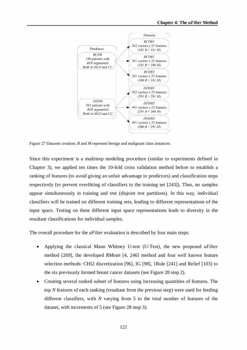
Chapter 4: The uFilter Method
121
Figure 27 Datasets creation; B and M represent benign and malignant class instances.
Since this experiment is a multistep modeling procedure (similar to experiments defined in
Chapter 3), we applied ten times the 10-fold cross validation method before to establish a
ranking of features (to avoid giving an unfair advantage to predictors) and classification steps
respectively (to prevent overfitting of classifiers to the training set [243]). Thus, no samples
appear simultaneously in training and test (disjoint test partitions). In this way, individual
classifiers will be trained on different training sets, leading to different representations of the
input space. Testing on these different input space representations leads to diversity in the
resultant classifications for individual samples.
The overall procedure for the uFilter evaluation is described by four main steps:
Applying the classical Mann Whitney U-test (U-Test), the new proposed uFilter
method [269], the developed RMean [4, 246] method and four well known feature
selection methods: CHI2 discretization [96], IG [98], 1Rule [241] and Relief [103] to
the six previously formed breast cancer datasets (see Figure 28 step 2).
Creating several ranked subset of features using increasing quantities of features. The
top N features of each ranking (resultant from the previous step) were used for feeding
different classifiers, with N varying from 5 to the total number of features of the
dataset, with increments of 5 (see Figure 28 step 3).

Chapter 4: The uFilter Method
122
Classifying the generated ranked subset of features using FFBP neural network [244],
SVM [77, 244], LDA [213] and NB [245] classifiers for a comparative analysis of
AUC scores. All comparisons were using the Wilcoxon statistical test [249, 251] to
assess the meaningfulness of differences between classification schemes (see Figure
28 step 3).
Selecting the best classification scheme on datasets (BCDR1, BCDR2, BCDR3,
DDSM1, DDSM2 and DDSM3), and thus the best subset of features.
Figure 28 Experimental workflow.
In the last step of the experiment, we determined the feature relevance analysis using a two-
step procedure involving (1) selecting the best subset of features for each dataset, and (2)
performing a redundancy analysis based on the Pearson correlation [253], to determine and
eliminate redundant features from relevant ones, and thus to produce the optimal subset of
features.
In contrast to the work of Ghazavi and Liao [209], we decided to employ the correlation
analysis as a complementary step to the uFilter procedure, instead to an evaluation function
for features selection, because in real domains many features have high correlations and thus
many are (weakly) relevant and should not be removed [270]. Also, some variables may have
a low rank because they are redundant and yet be highly relevant [56].

Chapter 4: The uFilter Method
123
4.5. Results and Discussions
4.5.1. Comparison between uFilter and U-Test Methods
The statistical comparison between uFilter and U-Test methods considered only features
subsets formed by the top 10 features (empirical threshold) of each ranking. We used a total
of 48 ranked subsets of features containing image-based features for feeding four machine
learning classifiers. With this, a head-to-head statistical comparison based on the mean of
AUC performances over 100 runs produced inspiring results. Figure 29 shows a boxplot
graph representing the statistical comparison (p<0.05) based on the mean of AUC scores
between both methods for all classification schemes.
Figure 29 Head-to-head comparison between uFilter (uF) and U-Test (uT) methods using the top 10 features of each ranking; blue and red filled box represents significant difference (p<0.05) in the AUC performance.

Chapter 4: The uFilter Method
124
Results on Balanced Datasets
The best classification scheme for BCDR1 dataset was formed by the uFilter method and the
SVM classifier (see Figure 29 b). The AUC value of 0.8369 was statistically superior to the
best AUC value (0.7995) obtained by the U-Test method when combined with the SVM
classifier. Also, this combination was statistically better than the remaining classification
schemes in the BCDR1 dataset (see Table 32).
For DDSM1 dataset, the best classification scheme was formed by the uFilter method and the
SVM classifier, reaching an AUC score of 0.80. However, this result did not provide
statistical evidence to be better than the combination of the U-Test method and the SVM
classifier, which reached an AUC score of 0.7838 (see Figure 29 b). This combination
statistically outperformed only three classification schemes for DDSM1 dataset (see Table
32).
Table 32 Summary of the Wilcoxon Statistical test among all classification schemes for BCDR1 and DDSM1
datasets.
Dataset Best scheme AUC Other scheme AUC Wilcoxon (α= 0.05)
BCDR1 uFilter+SVM 0.8369 U-Test+SVM 0.7995 p<0.01
uFilter+FFBP 0.8088 p<0.01
U-Test+FFBP 0.7938 p<0.01
uFilter+LDA 0.7906 p<0.01
U-Test+LDA 0.7968 p<0.01
uFilter+NB 0.7814 p<0.01
U-Test+NB 0.7840 p<0.01
DDSM1 uFilter+SVM 0.80 U-Test+SVM 0.7838 p=0.1390
uFilter+FFBP 0.7868 p=0.0986
U-Test+FFBP 0.7925 p=0.5149
uFilter+LDA 0.7567 p<0.01
U-Test+LDA 0.7832 p=0.0624
uFilter+NB 0.7277 p<0.01
U-Test+NB 0.7288 p<0.01

Chapter 4: The uFilter Method
125
Results on Unbalanced Datasets
The best classification scheme for BCDR2 dataset was formed by the uFilter method and the
FFBP neural network, reaching an AUC score of 0.8350. This result was statistically superior
to the obtained result by the combination of the U-Test method with the FFBP neural
network, which provided an AUC score of 0.7578 (see Figure 29 e). In this dataset other
classification schemes using the uFilter method stretched satisfactory results with no
statistical difference respect to the best scheme (see Table 33).
Besides, for DDSM2 dataset the best classification performance was obtained by the
combination of the uFilter and the FFBP neural network classifier; reaching AUC value of
0.8382 (see Figure 29 e). However, this result did not statistically outperform the obtained
result by the combination of the U-Test method and the FFBP neural network (AUC value of
0.8308). The comparison among all classification schemes for DDSM2 dataset indicated that
the best combination (higher AUC value) was almost statistically superior in all cases (see
Table 33).
Table 33 Summary of the Wilcoxon Statistical test among all classification schemes for BCDR2 and DDSM2
datasets.
Dataset Best scheme AUC Other scheme AUC Wilcoxon (α= 0.05)
BCDR2 uFilter+FFBP 0.8350 U-Test+FFBP 0.7578 p<0.01
uFilter+SVM 0.8332 p=0.6086
U-Test+SVM 0.7482 p<0.01
uFilter+LDA 0.8296 p=0.5849
U-Test+LDA 0.7613 p<0.01
uFilter+NB 0.8219 p=0.1546
U-Test+NB 0.7246 p<0.01
DDSM2 uFilter+FFBP 0.8382 U-Test+FFBP 0.8308 p=0.4923
uFilter+SVM 0.7782 p<0.01
U-Test+SVM 0.7844 p<0.01
uFilter+LDA 0.8296 p=0.7031
U-Test+LDA 0.7881 p<0.01
uFilter+NB 0.7511 p<0.01
U-Test+NB 0.8057 p<0.01

Chapter 4: The uFilter Method
126
The best classification performance for BCDR3 dataset was provided by the combination of
the uFilter method and the FFBP neural network classifier, accomplishment an AUC score of
0.8850 (see Figure 29 i). This result was statistically superior to the obtained result by the
combination of the U-Test method and the FFBP neural network, which achieved an AUC
score of 0.87. With the exception of the scheme formed by the U-Test method and the LDA
classifier, which attained a similar AUC performance (0.8725), the best scheme statistically
outperformed the remaining classification schemes (see Table 34).
In the DDSM3 dataset, the best classification scheme was formed by the combination of the
uFilter method and the LDA classifier for an AUC value of 0.7819. This classification result
showed significant difference with respect to the classification result provided by the
combination of the U-Test method with the LDA classifier, which reached an AUC value of
0.7328 (see Figure 29 k). Also, the best combination statistically outperformed other obtained
results using the U-Test method in the classification scheme, and does not indicated statistical
evidences of being better than other uFilter combinations (see Table 34).
Table 34 Summary of the Wilcoxon Statistical test among all classification schemes for BCDR3 and DDSM3
datasets.
Dataset Best scheme AUC Other scheme AUC Wilcoxon (α= 0.05)
BCDR3 uFilter+FFBP 0.8850 U-Test+FFBP 0.87 p<0.01
uFilter+SVM 0.8386 p<0.01
U-Test+SVM 0.8207 p<0.01
uFilter+LDA 0.8621 p<0.01
U-Test+LDA 0.8725 p=0.2131
uFilter+NB 0.8152 p<0.01
U-Test+NB 0.8477 p<0.01
DDSM3 uFilter+LDA 0.7819 U-Test+LDA 0.7328 p<0.01
uFilter+FFBP 0.7806 p=0.9386
U-Test+FFBP 0.6266 p<0.01
uFilter+SVM 0.7795 p=0.8441
U-Test+SVM 0.7393 p<0.01
uFilter+NB 0.7706 p=2047
U-Test+NB 0.6467 p<0.01

Chapter 4: The uFilter Method
127
A head-to-head comparison between the proposed uFilter method and the classical Mann
Withney U-test (U-Test) is well demonstrated in the experiments reported here. As it is shown
in Tables 32, 33 and 34, the uFilter method statistically outperformed the U-Test method in a
50% (blue filled box); tied in a 37.5% (green filled box) and lost in a 12.5% (red filled box) of
the 24 considered scenarios (see Figure 29).This circumstance could be related with the
assigned weights to each feature in the ranking, e.g. in the BCDR1 dataset, the uFilter method
considered the f20 feature (perimeter) as the most relevant feature, meanwhile the U-Test
method considered it as irrelevant. A similar situation occurs with the f37 feature (Area),
which was ranked in the top five features by the uFilter and irrelevant by the U-Test method
respectively. According to the ACR [7], MC lesions are tiny bright dots in the breast, and
masses are very often obscure and greater than MCs. Hence the perimeter and area are
important features for discriminating between both lesions. It is clear that the U-Test method
underestimated both features on unbalanced datasets.
In addition, for unbalanced datasets this fact could be associated to the Mann-Whitney test
criterion [252], which is based on the magnitude of the relationship between both samples
(benign and malignant instances). In the BCDR2, DDSM2, BCDR3 and DDSM3 datasets
most of the benign instances are greater than most of the malignant instances or vice versa
and this would be evidence against random mixing. Therefore, the U-Test method would tend
to discredit the null hypothesis of identical distribution [265] and underrate the features
weight (like in the balanced datasets). The opposite occur with the uFilter method, which
computes the separability between both samples, independently of the number of benign and
malignant instances.
4.5.2. Performance of uFilter versus Classical Feature Selection Methods
This section aims to compare the new developed uFilter method against four well known
(established) feature selection methods. A total of 720 ranked subsets of image-based features
were analyzed and the straightforward statistical comparison based on the mean of AUC
performances over 100 runs highlighted interesting results for balanced and unbalanced
datasets (see Figure 30).

Chapter 4: The uFilter Method
128
Figure 30 Behavior of the best classification schemes when increasing the number of features on each dataset.
Results on Balanced Datasets
On the BCDR1 dataset, the best classification scheme was obtained when we combine the
uFilter method and the SVM classifier using 10 features, obtaining an AUC score of 0.8369.
The statistical comparison against the other feature selection methods did not provide
significant difference in term of AUC scores: CHI2 discretization (AUC=0.8325, p=0.6717),
IG (AUC=0.8324, p=0.6725), 1Rule (AUC=0.8310, p=0.6053) and Relief (AUC=0.8316,
p=0.6190). However, the uFilter method reached this result using the top 10 features, while
the other methods required a total of 20 features (see Figure 30 a).
On the DDSM1 dataset, the combination of the uFilter method and the SVM classifier using
the top 10 features provided the best classification performance obtaining an AUC value of
0.8004. This result was not statistically superior to the obtained result by the CHI2
discretization (AUC=0.7893, p=0.2684), IG (AUC=0.7893, p=0.2840) and 1Rule methods
(AUC=0.79, p=0.3450), but it was better than the Relief method (AUC=0.7821, p<0.05).
Similar to the BCDR1 dataset, the uFilter method reached this result using the top 10
features, while the other methods required a total of 20 features (see Figure 30 d).

Chapter 4: The uFilter Method
129
Results on Unbalanced Datasets
The higher classification performance in the BCDR2 dataset was achieved by the combination
of the uFilter method and the FFBP neural network classifier with a total of 10 features,
obtaining an AUC value of 0.8350. However, this result was not statistically superior to the
obtained results by the remaining feature selection methods using the same number of features
(see Figure 30 b): CHI2 discretization (AUC=0.8342, p=0.7590), IG (AUC=0.8320,
p=0.8022), 1Rule (AUC=0.8259, p=0.8259) and Relief (AUC=0.8344, p=0.8402). Similar to
the BCDR2 dataset, the higher classification performance in the DDSM2 dataset was obtained
by the combination of the uFilter method and the FFBP neural network classifier using a total
of 10 features, accomplishment an AUC of 0.8382 (see Figure 30 e). This result did not
provide statistical evidences of an AUC improvement respect to the CHI2 discretization
(AUC=0.8301, p=0.8079), IG (AUC=0.8374, p=0.9076), 1Rule (AUC=0.8326, p=0.7470)
and Relief methods (AUC=0.8315, p=0.3884).
On the other hand, the best classification scheme for the BCDR3 dataset was formed by the
combination of the uFilter method and the FFBP neural network classifier using a total of 10
features (see Figure 30 c). The AUC value of 0.8850 was statistically superior respect to the
obtained result by the CHI2 discretization (AUC=0.8444, p<0.01), IG (AUC=0.8465,
p<0.01), 1Rule (AUC=0.8454, p<0.01) and Relief methods (AUC=0.8347, p<0.01).
On the DDSM3 dataset, the best classification performance was obtained by the combination
of the IG method and the FFBP neural network classifier using 15 features (AUC value of
0.7945). The AUC-based comparison against the other classification schemes using less
number of features (10) indicated no significant difference in the classification performance
(see Figure 30 f): CHI2 discretization (AUC=0.7798, p=0.0729), 1Rule (AUC=0.7776,
p=0.0551), Relief (AUC=0.7933, p=0.9717) and uFilter (AUC=0.7806, p=0.0796).
The global comparison demonstrated that uFilter method statistically outperformed the CHI2
discretization, IG, 1Rule and Relief methods on BCDR1, DDSM1 and BCDR3 datasets, and
it was statistically similar on BCDR2, DDSM2 and DDSM3 datasets while requiring less
number of features. This circumstance could be related to the particular nature of employed
feature selection methods and datasets respectively. We used datasets without any type of data
normalization, and some methods could lead to non-reliable results e.g. the CHI2
discretization (which used the chi-square statistical test as the main evaluation function), IG

Chapter 4: The uFilter Method
130
(which is an entropy-based feature evaluation), and 1Rule (which is not likely to enhance the
performance of classification schemes that require a search space of greater complexity)
methods provided the worst results on BCDR1, DDSM1 and BCDR3 datasets (see Figure 30).
In contrast, the Relief method computes the feature’s weight based on a different semantic
independent of data normalization (distance to nearest hit and nearest miss), and this explains
the good performance of the Relief method in almost all datasets (see Figure 30). The
satisfactory results obtained by the uFilter were expected since it is a non-parametric method
and thus is tolerant to non-normalized data.
Concerning classifiers performance, results show that the selection of the most appropriate
classifier is dependent on the dataset and the feature selection method (see Figure 30). For
balanced datasets, the best results were obtained with de SVM classifier; meanwhile for
unbalanced datasets were obtained with the FFBP neural network classifier (see Figure 30).
These results were expected since the SVM classifier is based on the definition of an optimal
hyperplane [244], and for a less complex features space (e. g. balanced datasets), it could
easily find the corresponding linear decision boundary. On the other hand, for a more
complex features space such as those presented on unbalanced datasets, the FFBP neural
network has demonstrated to be capable of generalizing [244].
4.5.3. Performance of uFilter versus RMean Feature Selection Method
This section aims to present a head-to-head comparison between the contributions of this
thesis: the new uFilter proposed method, which improves a non-parametric statistical test and
the RMean method, which is based on the combination of four classical feature selection
methods (see Chapter 3 for technical information).
Analogous to the previous section, we analyzed a total of 720 ranked subsets of features
containing image-based features and a direct statistical comparison based on the mean of
AUC performances over 100 runs was carried out. The Figure 31 shows the behavior (AUC
variability when increasing the number of features) of the best classification scheme and the
performance of the uFilter and RMean feature selection methods, for each formed dataset.
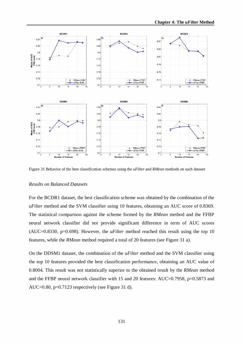
Chapter 4: The uFilter Method
131
Figure 31 Behavior of the best classification schemes using the uFilter and RMean methods on each dataset
Results on Balanced Datasets
For the BCDR1 dataset, the best classification scheme was obtained by the combination of the
uFilter method and the SVM classifier using 10 features, obtaining an AUC score of 0.8369.
The statistical comparison against the scheme formed by the RMean method and the FFBP
neural network classifier did not provide significant difference in term of AUC scores
(AUC=0.8330, p=0.698). However, the uFilter method reached this result using the top 10
features, while the RMean method required a total of 20 features (see Figure 31 a).
On the DDSM1 dataset, the combination of the uFilter method and the SVM classifier using
the top 10 features provided the best classification performance, obtaining an AUC value of
0.8004. This result was not statistically superior to the obtained result by the RMean method
and the FFBP neural network classifier with 15 and 20 features: AUC=0.7958, p=0.5873 and
AUC=0.80, p=0.7123 respectively (see Figure 31 d).
Chapter 4: The uFilter Method
132
Results on Unbalanced Datasets
The higher classification performance in the BCDR2 dataset was achieved by the combination
of the uFilter method and the FFBP neural network classifier with a total of 10 features,
obtaining an AUC value of 0.8350. However, this result was not statistically superior to the
obtained results by the RMean method and the FFBP neural network classifier using the same
number of features, which achieved an AUC value of 0.8288, p=0.5922 (see Figure 31 b).
Similar to the BCDR2, the higher classification performance in the DDSM2 dataset was
obtained by the combination of the uFilter method and the FFBP neural network classifier
using a total of 10 features, accomplishment an AUC of 0.8382 (see Figure 31 e). This result
did not provide statistical evidences of an AUC improvement respect to the RMean
(AUC=0.8352, p=0.7215).
On the BCDR3, the best classification performance was reached by the combination of the
uFilter method and the FFBP neural network classifier using a total of 10 features (see Figure
31 c). The AUC value of 0.8850 was statistically superior respect to the obtained result by the
RMean method and the FFBP neural network classifier (AUC=0.8544, p<0.01).
On the other hand, the higher performance for the DDSM3 dataset was formed by the
combination of the RMean method and the FFBP neural network classifier using a total of 10
features (see Figure 31 f). The AUC value of 0.7957 was not statistically superior respect to
the obtained result by the uFilter method (AUC=0.7806, p=0.3112),
The head-to-head comparison demonstrated that uFilter method statistically outperformed the
RMean method on BCDR1, DDSM1 and BCDR3 datasets, and it was statistically similar on
BCDR2, DDSM2 and DDSM3 datasets. This result was expected since the RMean method is
based on the combination of the CHI2 discretization, IG, 1Rule and Relief feature selection
methods, which were also statistically outperformed by the uFilter method (see previous
subsection). It should be pointed out that RMean method is an ensemble method and will
inherit all the weaknesses presented on each baseline method.
4.5.4. Analysis of the Ranked Features Space
Many methods of variable subset selection are sensitive to small perturbations of the
experimental conditions. If the data has redundant variables, different subsets of variables
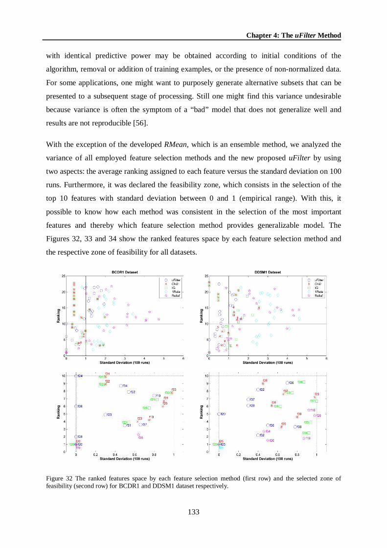
Chapter 4: The uFilter Method
133
with identical predictive power may be obtained according to initial conditions of the
algorithm, removal or addition of training examples, or the presence of non-normalized data.
For some applications, one might want to purposely generate alternative subsets that can be
presented to a subsequent stage of processing. Still one might find this variance undesirable
because variance is often the symptom of a “bad” model that does not generalize well and
results are not reproducible [56].
With the exception of the developed RMean, which is an ensemble method, we analyzed the
variance of all employed feature selection methods and the new proposed uFilter by using
two aspects: the average ranking assigned to each feature versus the standard deviation on 100
runs. Furthermore, it was declared the feasibility zone, which consists in the selection of the
top 10 features with standard deviation between 0 and 1 (empirical range). With this, it
possible to know how each method was consistent in the selection of the most important
features and thereby which feature selection method provides generalizable model. The
Figures 32, 33 and 34 show the ranked features space by each feature selection method and
the respective zone of feasibility for all datasets.
Figure 32 The ranked features space by each feature selection method (first row) and the selected zone of feasibility (second row) for BCDR1 and DDSM1 dataset respectively.

Chapter 4: The uFilter Method
134
In the BCDR1 dataset, the uFilter method considered the top 10 features inside the feasibility
zone. Also, the obtained results by the CHI2 discretization and IG methods were close to the
uFilter method, ranking 8 and 7 features inside this zone respectively. The worst results were
presented by the Relief and 1Rule methods, the first one ranked only 2 features inside the
feasibility zone and the second ranked the top 10 features out of this zone (see Figure 32
second row).
For the DDSM1 dataset, the best result was obtained by the uFilter method, which ranked 9
features inside the feasibility zone. The CHI2 discretization and IG methods considered both
7 features and, the Relief and 1Rule methods provided the worst results, ranking 5 and 1
feature inside the feasibility zone respectively (see Figure 32 second row).
In the BCDR2 dataset, the uFilter was slightly superior (selected 9 features) against the CHI2
discretization, IG and Relief methods, which obtained very close results. These methods
considered 7, 8 and 7 features inside the feasibility zone respectively. Likewise in the BCDR1
dataset, the 1Rule method resulted in worst without any selection inside the feasibility zone
for BCDR2 dataset (see Figure 33 second row).
Besides, for the DDSM2 dataset, the best results were obtained by the uFilter, CHI2
discretization and IG methods. All of them ranked 8 features inside the feasibility zone. In
contrast, the Relief and 1Rule methods considered only 2 and 3 features within this zone
respectively. These latter results were the worst in this dataset (see Figure 33 second row).

Chapter 4: The uFilter Method
135
Figure 33 The ranked features space by each feature selection method (first row) and the selected zone of feasibility (second row) for BCDR2 and DDSM2 dataset respectively.
In the BCDR3 dataset, the best result was provided by the uFilter method, which ranked 7
features inside the feasibility zone. The CHI2 discretization, IG, 1Rule and Relief methods
obtained very close results among them (5, 4, 4 and 6 features respectively), but it were lower
respect to the uFilter method.
Moreover, for the DDSM3 dataset, the best results were obtained by the uFilter and CHI2
discretization methods, both ranked 9 features inside the feasibility zone. The IG method
considered 7 features inside this zone and, the worst results were obtained by the 1Rule and
Relief methods, which ranked 1 and 5 features respectively (see Figure 34 second row).

Chapter 4: The uFilter Method
136
Figure 34 The ranked features space by each feature selection method (first row) and the selected zone of feasibility (second row) for BCDR3 and DDSM3 dataset respectively.
It should be pointed out that the uFilter method was the most consistent in ranking features
with less variance among all feature selection methods for all datasets, which mean it is
capable of provided models that generalize well. In contrast, the 1Rule was the worst method;
it ranked the features with high variance in the majority of datasets.
4.5.5. Feature Relevance Analysis
The results showed in previous section clearly provide experimental evidence that the uFilter
method provided ranked subsets of features with higher discriminant potential. It
approximates the set of relevant features by selecting a subset from the top 10 features of each
ranking list. According to its linear time complexity in terms of the dimensionality N (total of
features), the uFilter method is efficient for high-dimensional data. However, it is incapable
of removing redundant features because it is an individual evaluator of features (i.e. it assigns
weights according to their degrees of relevance [56]) and as long as features are considered
relevant to the class, they will all be selected even though many of them are highly correlated

Chapter 4: The uFilter Method
137
to each other (redundant). In this case, a validation of features’ subsets through a redundancy
analysis is convenient.
Features Subset Validation
To efficiently find an optimal subset of features we introduced an analysis of redundancy to
decrease the size of the subset of features and keeping prediction accuracy. We achieved this
goal using a two-step procedure involving: (1) selecting the best subset of features for each
dataset, and (2) performing the redundancy analysis based on the Pearson correlation [253] to
determine and eliminate redundant features from relevant ones, and thus to produce the
optimal subset of features.
In order to correctly interpret the results, John and Kohavi in [50] defined two degrees of
relevance: strong and weak. Strong relevance implies that the feature is indispensable in the
sense that it cannot be removed without loss prediction accuracy. Weak relevance (redundant
and non-redundant) implies that the feature can sometimes contribute to prediction accuracy.
Thus, features are relevant if they are both strongly or weakly relevant and irrelevant
otherwise. Irrelevant features can never contribute to prediction accuracy, by definition.
As it is shown in Figure 30 and described in previous section, the relevance analysis based on
the proposed uFilter method provided discriminant subsets of features by removing irrelevant
ones. Hence, these subsets of features were used as the starting point for the redundancy
analysis. Table 35 summarizes the redundancy analysis based on the Pearson correlation [253]
for each selected subset of features. It should be pointed out that only higher correlation
values were considered in this analysis (more than 0.5 on both positive and negative
direction).

Chapter 4: The uFilter Method
138
Table 35 Summary of the redundancy analysis.
Dataset Best subset of features
Redundant features
c-Pearson Weakly relevant
Strongly relevant
BCDR1
f20,f28,f31,f37,f23,f26,f19,f22,f34, f24
f37=f20 f26=f23,f19 f19=f23 f34=f22
0.79 0.96, -0.92 -0.84 -0.62
f20,f31(+),f23,
f22, f24 f28
BCDR2
f30,f38,f37,f20,f28,f31,f22,f29,f27,f24
f30=f38,f29, f27 f37=f20 f29=f38 f24=f22
0.99, 0.56, 0.56 0.89 0.55 0.75
f38,f28(+),
f31(+),f22,f27
f20
BCDR3
f23,f26,f19,f20,f28,f34,f31,f38,f35,f29
f26=f23,f19, f38 f19=f23,f38 f34=f28 f29=f23,f26,f19,f38
0.97,-0.94,0.56 -0.85,-0.62 -0.75 0.50, 0.57,-0.62, 0.99
f23,f20(+),f28,
f31(+),f38
f35
DDSM1
f25,f32,f35,f39,f20,f28,f37,f22,f26, f31
f39=f25,f32,f35 f37=f20 f22=f20, f31 f31=f28
f32=f35
0.85, 0.94, 0.94 0.93 0.56,-0.71 -0.79 0.99
f25(+),f20,f28,
f26(+),f35
-
DDSM2 f23,f35,f32,f39,f25,f19,f16,f21,f28,f24
f39=f35,f32,f25,f28,f24 f25=f35,f32,f24 f28=f25
0.97,0.98,0.89,0.71,0.51 0.92,0.92,0.61 0.68
f35,f32,f19(+),
f16(+),f21
(+), f24
f23
DDSM3
f25,f20,f37,f39,f32,f26, f35,f28, f34, f22
f37=f25 f39=f25,f32,f35 f32=f25,f35 f28=f25,f20,f34,f22
0.84 0.78,0.92,0.91 0.85,0.99 0.60,0.56,0.57,0.76
f25,f26(+),f35,
f34, f22 f20
(+)Weakly relevant features but non-redundant; c-Pearson is the value of correlation of Pearson.
Correlated features are considered redundant (see Table 35). Therefore, only one of them in
the correlated pair is selected together with the non-correlated features to form the weakly
relevant subset of features. Hence each weakly relevant subset of features was used for
selecting the strongly relevant ones.
In the BCDR1 dataset, the Entropy (f28) feature was selected as the strongly relevant feature
because its absence in the final subset of features significantly decreased the AUC
performance from 0.8315 to 0.791 (p<0.01). In the BCDR2 and DDSM3 datasets, the
Perimeter (f20) feature constituted the strongly relevant feature. Its participation in the final
subset significantly increased the AUC performance from 0.81 to 0.835 (p<0.01) and 0.7521
to 0.7806 (p<0.01) respectively.
For the BCDR3 dataset, the Mean (f35) feature was considered as the strongly relevant feature
because its absence significantly reduced the classification performance from an AUC value
of 0.885 to 0.8395 (p<0.01). Besides, in the DDSM2 dataset, the strongly relevant feature was
the Roughness (f23); this feature contributed to a significantly increment of 0.07 (p<0.01) in

Chapter 4: The uFilter Method
139
the AUC performance when it is included in the final subset (AUC value of 0.8382 versus
0.7727 when is left out). Only in the DDSM1 dataset no feature appears as strongly relevant,
which means that all features in this subset contributed with similar effort in the classification
model. It should be pointed out that removed features can be inferred from Table 37.
According to the relevant definition of John and Kohavi [270], we put together both weakly
and strongly relevant features to form the optimal subset of features. These subsets were
evaluated using the same machine learning classifier employed in the evaluation of its
precedent subsets of features (for further comparison). Therefore, optimal subset of features
for BCDR1 and DDSM1 datasets used the SVM classifier, and for BCDR2, BCDR3, DDSM2
and DDSM3 datasets used the FFBP neural network respectively. Table 36 summarizes the
AUC-based statistical comparison (using the Wilcoxon statistical test [249, 250]) between the
best subset of features selected by the uFilter method, and its corresponding optimal subset of
features after the redundancy analysis.
Table 36 AUC-based statistical comparison between the best and optimal subset of features.
Dataset Best subset of features AUC Weakly + Strongly AUC Wilcoxon
(α=0.05)
BCDR1 f20,f28,f31,f37,f23,f26,f19,f22,f34,f24 0.839 f20,f31(+),f23,f22,f24,f28 0.8315 p=0.811
BCDR2 f30,f38,f37,f20,f28,f31,f22,f29,f27,f24 0.835 f38,f28(+),f31
(+),f22,f27,f20 0.8413 p=0.841
BCDR3 f23,f26,f19,f20,f28,f34,f31,f38,f35,f29 0.885 f23,f20(+),f28,f31
(+),f38,f35 0.8821 p=0.918
DDSM1 f25,f32,f35,f39,f20,f28,f37,f22,f26,f31 0.8004 f25(+),f20,f28,f26
(+),f35 0.8001 p=0.982
DDSM2 f23,f35,f32,f39,f25,f19,f16,f21,f28,f24 0.8382 f35,f32,f19(+),f16
(+),f21(+),f24,f23 0.8435 p=0.757
DDSM3 f25,f20,f37,f39,f32,f26,f35,f28,f34,f22 0.7806 f25,f26(+),f35,f34,f22,f20 0.7759 p=0.685
(+)Weakly relevant features but non-redundant.
From Table 36, it is possible to conclude that only two optimal subsets of features provided a
slight increment in terms of AUC performance, but these results were not significantly
superior. Furthermore, the remaining optimal subsets of features did not provide significance
difference in the AUC performance.
Concerning redundancy analysis, redundant features were detected on every dataset, which
means there are some variables providing similar information to the classifier, and thus it is
unnecessarily increasing the complexity of the classification model. With the exception of the
DDSM1 dataset, it was possible to find the most relevant feature for all the datasets. In the
case of the BCDR2 dataset, the Perimeter (f20) feature was selected as the most appropriated
strongly relevant feature, however it has a unique correlation with the Area (f37) feature (c-
Pearson value of 0.89). In this case, it is possible to interchange both features (f20 or f37) and

Chapter 4: The uFilter Method
140
select only one of them as the most relevant feature (see Table 36). Likewise, in the DDSM3,
the Perimeter (f20) feature was selected as the most relevant feature and is correlated with the
Entropy (f28) feature (c-Pearson value of 0.56), but the Entropy (f28) feature is also correlated
with others features: Maximum (f25), Correlation (f34) and Standard deviation (f22); under this
situation, the selected Perimeter (f20) feature is the only one which can be elected as the most
relevant feature. This particular effect on both datasets could be explained by the c-Pearson
values; the correlation value between Perimeter (f20) and Area (f37) was high (unique
correlation) meanwhile the correlation value between Perimeter (f20) and Entropy (f28) was
low (multi-correlation). It means that it is possible interchanging most relevant features only
if there is a unique and strong correlation between them.
We considered strongly relevant features as the most important features: Perimeter (f20),
Entropy (f28), Mean (f35) and Roughness (f23). They consistently appeared at least 3 times
(each one) on the six optimal features subsets (see Table 36). This result was expected due to
the binary classification problem (benign-malignant classes) investigated in this work. The
perimeter and roughness features are considered significant shape descriptors for masses
classification i.e. benign masses possess smooth, round, or oval shapes with possible
macrolobulations, as opposed to malignant tumors which typically exhibit rough contours
with microlobulations, spiculations, and concavities [7]. On the other hand, the entropy and
mean features are more likely to be employed for MC classification i.e the entropy is a feature
that represents the texture of the background tissue where the calcifications are embedded in
[129, 140]; meanwhile, the mean is an intensity statistics descriptor used with higher
frequency [78, 137] because MCs are tiny brighter dots [7].
Regarding classification performances, the proposed uFilter method was able to produce
subsets of features with higher discriminant potential and the redundancy analysis did not
improve the prediction accuracy, but decreased the size of the subset of features without
significantly decreasing the performance. This result was expected since the uFilter method is
an individual evaluator of features (filter paradigm) and it ignores the feature dependencies.
This is the main drawback of individual features evaluator methods as is the case of uFilter.

141
Conclusions
This chapter presents an overview of the work that we have developed in the scope of this
thesis. Also we summarized the main contributions, limitations and future work.
5.1. Thesis Overview
Breast imaging, which is fundamental to cancer risk assessment, detection, diagnosis and
treatment, is undergoing a paradigm shift: the tendency is to move from a primarily
qualitative interpretation to a more quantitative-based interpretation model. In term of
diagnosis, the mammography and the double reading of mammograms are two useful and
suggested techniques for reducing the proportion of missed cancers. But the workload and
cost associated are high.
Breast Cancer CADx systems is a more recent technique, which have been improved both the
AUC performance of radiologists (see Chapter 1, Table 1) and the classification of cancer in
its early stages (see Chapter 2, Table 12). Despite these prominent results, the performance of
current and future commercial CADx systems still needs to be improved so that they can meet
the requirements of clinics and screening centers [20, 94].
CH
AP
TER
Chapter 5: Conclusions
142
The feature selection constitutes one of the most important steps in the lifecycle of Breast
Cancer CADx systems. It presents many potential benefits such as: facilitating data
visualization and data understanding, reducing the measurement and storage requirements,
reducing training and utilization times and, defining the curse of dimensionality to improve
the predictions performance. It is therefore convenient that feature selection methods are fast,
scalable, accurate and possibly with low algorithmic complexity.
This thesis was motivated by the need of developing new feature selection methods to provide
more accurate and compact subsets of features to feed MLCs supporting breast cancer
diagnosis. After some months of research studying previous developed approaches existing at
that time, we realized that most of the developed approaches were focused on the wrapper or
hybrid paradigm and, in fewer degrees on filter paradigm (see Chapter 2, section “Feature
Selection Methods”).
We considered exploring the filter paradigm (univariate and multivariate) over the wrappers
or hybrid models; because filter methods provide lower algorithmic complexity, faster
performance and are independent of classifiers. It means that filter methods analyze the
characteristics of data for ranking the entire space of features, while the wrappers or hybrid
methods are extremely dependent of classifiers for selecting a satisfactory subset of features.
The principal limitation of univariate filter methods is that they ignore the dependencies
among features and assume a given distribution (Gaussian in most cases) from which the
samples (observations) have been collected. In addition, assuming a Gaussian distribution
includes the difficulties to validate distributional assumptions because of small sample sizes.
On the other hand, multivariate filters methods overcome the problem of ignoring feature
dependencies introducing redundancy analysis (models feature dependencies) at some degree,
but the improvements are not always significant: domains with large numbers of input
variables suffer from the curse of dimensionality and multivariate methods may overfit the
data. Also, multivariate methods have shown to be slower and less scalable than univariate
methods. These limitations on existing filter methods may lead the Breast Cancer CADx
methods to classification performances bellow of its potential.

Chapter 5: Conclusions
143
5.2. Main Contributions and Future Work
While the results achieved in this thesis have been outlined before, into the developed
chapters, to follow we summarized the main contributions:
Contribution 1: A new ensemble feature selection method (named RMean) supported on the
filter paradigm for indexing relevant features extracted from mammographic pathological
lesions (image-based and clinical features).
The RMean method used four feature selection methods with different evaluation function
from the fillter paradigm: the CHI square discretization based on the chi-square statistic
function, Information Gain based on the information measure, 1Rule based on rules as
principal evaluation functions and Relief based on the distance measure. The application of
these methods produces four different ranking of features (one by each applied feature
selection method). Then, the mean position of each feature along the four features ranking
was computed and, a new ranking was created using the mean position of features as indexing
criterion. When applied to the breast cancer datasets under study, the subsets of ranked
features produced by using the RMean method improved the AUC performance in almost all
the explored machine learning classifiers.
Contribution 2: A new feature selection method (named uFilter) based on the Mann
Whitney U-test for ranking relevant features, which assess the relevance of features by
computing the separability between class-data distribution of each feature.
The uFilter is an innovative univariate filter method that improves the Mann Whitney U-test
for reducing dimensionality and ranking features in binary classification problems. It solves
some difficulties remaining on previous developed methods, such as: it is effective in ranking
relevant features independently of the samples sizes (tolerant to unbalanced training data); it
does not need any type of data normalization; and the most important, it presents a low risk of
data overfitting and does not incur the high computational cost of conducting a search through
the space of feature subsets as in the wrapper or embedded methods.
Contribution 3: An improvement in the performance of machine learning classifiers
supporting Breast Cancer CADx methods.

Chapter 5: Conclusions
144
Both feature selection methods (RMean and uFilter) were validated on breast cancer datasets
for further statistical comparison against other developed existing approaches. According to
the Wilcoxon statistic test, the ensemble RMean method (contribution 1) was the best on
selecting relevant features when compared against the four baseline feature selection methods.
It appeared consistently on all succeeds combinations for microcalcifications and masses
classification. Also, it improved the performance of mammography-based machine learning
classifiers. Despite the good performance of the RMean method, it still ignores the features
dependence and redundant information could lead to a non-desired classification result.
On the other hand, the uFilter method (contribution 2) performed better than the Mann
Whitney U-test (its theoretical basis) when applied to reduce and ranking features in binary
classification problems. uFilter was validated over six different (balanced and unbalanced)
datasets representative of two different breast cancer repositories. A head-to-head comparison
proved that the uFilter method significantly outperformed the U-Test method for almost all of
the classification schemes. It was superior in 50%; tied in a 37.5% and lost in a 12.5% of the
24 comparative scenarios. A global comparison against other four well known feature
selection methods demonstrated that uFilter statistically outperformed the remaining methods
on several datasets, and it was statistically similar on three datasets while requiring less
number of features. Moreover, a general comparison against the developed RMean method
also confirmed that the uFilter method was statistically superior on three datasets and
statistically similar on the remaining datasets. This method revealed competitive and
appealing cost-effectiveness results on selecting relevant features, as a support tool for breast
cancer CADx methods especially in unbalanced datasets contexts. Finally, the redundancy
analysis as a complementary step to the uFilter method provided us an effective way for
finding optimal subsets of features.
The development of these contributions provided important evidences to support the proposed
set of hypothesis in Chapter 1, Section 1.3. This can be reviewed in detail throughout the
Chapter 3 and Chapter 4 and, it is summarized here:
Hypothesis 1: Feature selection methods supported on the filter paradigm can be improved
by the creation of new ensemble methods. Experimental results in Section 3.6.2 statistically
demonstrated the satisfactory performance obtained by the developed RMean method when
compared to four well known (classical) feature selection methods of the filter paradigm.

Chapter 5: Conclusions
145
Hypothesis 2: Feature selection methods of the filter paradigm can be improved throughout
a new filtered function, which provides index of features with better separability between two
instance distributions. The theoretical description of the uFilter method (see Section 4.3) and
the experimental results reported in Section 4.5 constituted a sustain proof for the
corroboration of this hypothesis.
Hypothesis 3: Breast Cancer CADx systems can be advanced by the inclusion of a new
feature selection method that provides features with more discrimination power to yield better
AUC-based classifier performance. The AUC-based classification performance of MLCs was
always improved when using both the RMean and uFilter feature selection methods on breast
cancer datasets (see Section 3.6 and 4.5). However, the uFilter method demonstrated to be the
best, because it improved the main difficulties existing on univariate filter methods, including
the RMean method (Section 4.5).
In summary, the contributions of this thesis suggest that it possible to improve the feature
selection methods of the filter paradigm and the AUC-based classifier performance for breast
cancer CADx systems.
Future work will be aimed to three issues: (1) increasing the number of features in
benchmarking breast cancer datasets; (2) exploring the performance of uFilter method in
other knowledge domains and (3) extending the uFilter method allowing it to be used on
multiclass classification problems.

146
Bibliographic References
[1] M. D. Althuis, J. M. Dozier, W. F. Anderson, S. S. Devesa, and L. A. Brinton, "Global trends in breast cancer incidence and mortality 1973-1997", Int. J. Epidemiol., 2005, vol. 34, no. 2, pp. 405-412. http://dx.doi.org/10.1093/ije/dyh414.
[2] F. Kamangar, G. M. Dores, and W. F. Anderson, "Patterns of cancer incidence, mortality, and prevalence across five continents: defining priorities to reduce cancer disparities in different geographic regions of the world", Journal of clinical oncology, 2006, vol. 24, no. 14, pp. 2137-2150.
[3] V. Veloso, "Cancro da mama mata 5 mulheres por dia em Portugal", in CiênciaHoje, ed. Lisboa, Portugal, 2009.
[4] N. Pérez, M. A. Guevara, A. Silva, I. Ramos, and J. Loureiro, "Improving the performance of machine learning classifiers for Breast Cancer diagnosis based on feature selection", in Proceedings of the 2014 Federated Conference on Computer Science and Information Systems. M. Ganzha, L. Maciaszek, and M. Paprzycki (Eds.), IEEE, Warsaw, Poland, 2014, pp. 209-217. http://dx.doi.org/10.15439/2014F249.
[5] R. Ramos-Pollan, "Grid computing for breast cancer CAD. A pilot experience in a medical environment", in 4th Iberian Grid Infrastructure Conference, 2010, pp. 307-318.
[6] "What Is Breast Cancer?".http://www.breastcancer.org/symptoms/understand_bc/what_is_bc (Accessed: Jan 1, 2013).
[7] A. Committee, American College of Radiology (ACR) ACR BIRADS - Mammography, 4th ed. Reston, VA, 2003.
CH
AP
TER

Chapter 6: Bibliographic References
147
[8] H. Zonderland, T. Pope, Jr., and A. Nieborg, "The positive predictive value of the breast imaging reporting and data system (BI-RADS) as a method of quality assessment in breast imaging in a hospital population", European Radiology, 2004, vol. 14, no. 10, pp. 1743-1750. http://dx.doi.org/10.1007/s00330-004-2373-6.
[9] S. G. Orel, N. Kay, C. Reynolds, and D. C. Sullivan, "BI-RADS categorization as a predictor of malignancy", Radiology, 1999, vol. 211, no. 3, pp. 845-50.
[10] C. G. Ball, M. Butchart, and J. K. MacFarlane, "Effect on biopsy technique of the breast imaging reporting and data system (BI-RADS) for nonpalpable mammographic abnormalities", Can J Surg, 2002, vol. 45, no. 4, pp. 259-63.
[11] S. H. Taplin, L. E. Ichikawa, K. Kerlikowske, V. L. Ernster, R. D. Rosenberg, B. C. Yankaskas, et al., "Concordance of Breast Imaging Reporting and Data System Assessments and Management Recommendations in Screening Mammography", Radiology, 2002, vol. 222, no. 2, pp. 529-535. http://dx.doi.org/10.1148/radiol.2222010647.
[12] K. Bihrmann, A. Jensen, A. H. Olsen, S. Njor, W. Schwartz, I. Vejborg, et al., "Performance of systematic and non-systematic ('opportunistic') screening mammography: a comparative study from Denmark", J Med Screen, 2008, vol. 15, no. 1, pp. 23-6. http://dx.doi.org/10.1258/jms.2008.007055.
[13] M. H. Dilhuydy, "Breast imaging reporting and data system (BI-RADS) or French “classification ACR”: What tool for what use? A point of view", European Journal of Radiology, 2007, vol. 61, no. 2, pp. 187-191. http://dx.doi.org/10.1016/j.ejrad.2006.08.032.
[14] "Mammograms and Other Breast Imaging Procedures".http://www.cancer.org/treatment/understandingyourdiagnosis/examsandtestdescriptions/mammogramsandotherbreastimagingprocedures/mammograms-and-other-breast-imaging-procedures-mammo-report (Accessed: Jan 1, 2014).
[15] P. Boyle and B. Levin, World cancer report 2008: IARC Press, International Agency for Research on Cancer, 2008.
[16] M. M. Ng KH, "Advances in mammography have improved early detection of breast cancer", J Hong Kong Coll Radiol, 2003, vol. 6(3), no. pp. 126-131.
[17] "Digital vs. Film Mammography in the Digital Mammographic Imaging Screening Trial (DMIST): Questions and Answers".http://www.cancer.gov/cancertopics/factsheet/DMISTQandA (Accessed: Feb 2, 2013).
[18] D. Gur, "Digital Mammography: Do We Need to Convert Now?", Radiology, 2007, vol. 245, no. 1, pp. 10-11. http://dx.doi.org/10.1148/radiol.2451062078.
[19] E. D. Pisano, R. E. Hendrick, M. Yaffe, E. F. Conant, and C. Gatsonis, "Should Breast Imaging Practices Convert to Digital Mammography? A Response from Members of the DMIST Executive Committee1", Radiology, 2007, vol. 245, no. 1, pp. 12-13. http://dx.doi.org/10.1148/radiol.2451070393.

Chapter 6: Bibliographic References
148
[20] E. D. Pisano, C. Gatsonis, E. Hendrick, M. Yaffe, J. K. Baum, S. Acharyya, et al., "Diagnostic Performance of Digital versus Film Mammography for Breast-Cancer Screening", N Engl J Med, 2005, vol. 353, no. 17, pp. 1773-1783. http://dx.doi.org/10.1056/NEJMoa052911.
[21] W. Yang, "Digital mammography update", Biomed. Imag. Intervention, 2006, vol. 2, no. 4, pp. 45-12.
[22] M. Reddy and R. Given-Wilson, "Screening for breast cancer", Women's Health Medicine, 2006, vol. 3, no. 1, pp. 22-27.
[23] J. Shi, B. Sahiner, H.-P. Chan, J. Ge, L. Hadjiiski, M. A. Helvie, et al., "Characterization of mammographic masses based on level set segmentation with new image features and patient information", Medical Physics, 2008, vol. 35, no. 1, pp. 280-290.
[24] D. Guliato, R. M. Rangayyan, J. D. Carvalho, and S. A. Santiago, "Polygonal Modeling of Contours of Breast Tumors With the Preservation of Spicules", Biomedical Engineering, IEEE Transactions on, 2008, vol. 55, no. 1, pp. 14-20. http://dx.doi.org/10.1109/TBME.2007.899310.
[25] P. Delogu, M. Evelina Fantacci, P. Kasae, and A. Retico, "Characterization of mammographic masses using a gradient-based segmentation algorithm and a neural classifier", Computers in Biology and Medicine, 2007, vol. 37, no. 10, pp. 1479-1491. http://dx.doi.org/10.1016/j.compbiomed.2007.01.009.
[26] A. Karahaliou, S. Skiadopoulos, I. Boniatis, P. Sakellaropoulos, E. Likaki, G. Panayiotakis, et al., "Texture analysis of tissue surrounding microcalcifications on mammograms for breast cancer diagnosis", British Journal of Radiology, 2007, vol. 80, no. 956, pp. 648-656. http://dx.doi.org/10.1259/bjr/30415751.
[27] C. Varela, S. Timp, and N. Karssemeijer, "Use of border information in the classification of mammographic masses", Phys Med Biol, 2006, vol. 51, no. 2, pp. 425-41. http://dx.doi.org/10.1088/0031-9155/51/2/016.
[28] J. Wei, B. Sahiner, L. M. Hadjiiski, H.-P. Chan, N. Petrick, M. A. Helvie, et al., "Computer-aided detection of breast masses on full field digital mammograms", Medical physics, 2005, vol. 32, no. 9, pp. 2827-2838.
[29] E. S. d. Paredes, "Atlas of Mammography, 3rd ed", Radiology, 2009, vol. 252, no. 3, p. 663. http://dx.doi.org/10.1148/radiol.2523092526.
[30] "Breast Cancer Digital Repository".http://bcdr.inegi.up.pt/ (Accessed: Jan 1, 2014).
[31] J. S. Suri and R. M. Rangayyan, Recent advances in breast imaging, mammography, and computer-aided diagnosis of breast cancer vol. 155: SPIE press, 2006.
[32] C. H. Yip, R. A. Smith, B. O. Anderson, A. B. Miller, D. B. Thomas, E. S. Ang, et al., "Guideline implementation for breast healthcare in low- and middle-income countries: early detection resource allocation", Cancer, 2008, vol. 113, no. 8 Suppl, pp. 2244-56. http://dx.doi.org/10.1002/cncr.23842.

Chapter 6: Bibliographic References
149
[33] J. Brown, S. Bryan, and R. Warren, "Mammography screening: an incremental cost effectiveness analysis of double versus single reading of mammograms", BMJ (Clinical research ed.), 1996, vol. 312, no. 7034, pp. 809-812.
[34] R. Ramos-Pollan, M. A. Guevara-Lopez, C. Suarez-Ortega, G. Diaz-Herrero, J. M. Franco-Valiente, M. Rubio-Del-Solar, et al., "Discovering mammography-based machine learning classifiers for breast cancer diagnosis", J Med Syst, 2012, vol. 36, no. 4, pp. 2259-69. http://dx.doi.org/10.1007/s10916-011-9693-2.
[35] R. R. Pollán, "Improving multilayer perceptron classifiers AUC performance: An approach in biomedical image analysis for breast cancer CAD supported by eInfrastructures", Phd, Department of Informatics Engineering, Faculty of Engineering, University of Porto, 2011.
[36] A. Lauria, M. E. Fantacci, U. Bottigli, P. Delogu, F. Fauci, B. Golosio, et al., "Diagnostic performance of radiologists with and without different CAD systems for mammography", in Medical Imaging 2003, International Society for Optics and Photonics, 2003, pp. 51-56.
[37] L. H. Eadie, P. Taylor, and A. P. Gibson, "A systematic review of computer-assisted diagnosis in diagnostic cancer imaging", European Journal of Radiology, 2012, vol. 81, no. 1, pp. e70-e76. http://dx.doi.org/10.1016/j.ejrad.2011.01.098.
[38] J. J. Fenton, S. H. Taplin, P. A. Carney, L. Abraham, E. A. Sickles, C. D'Orsi, et al., "Influence of Computer-Aided Detection on Performance of Screening Mammography", New England Journal of Medicine, 2007, vol. 356, no. 14, pp. 1399-1409. http://dx.doi.org/10.1056/NEJMoa066099.
[39] I. Leichter, S. Fields, R. Nirel, P. Bamberger, B. Novak, R. Lederman, et al., "Improved mammographic interpretation of masses using computer-aided diagnosis", Eur Radiol, 2000, vol. 10, no. 2, pp. 377-83.
[40] Z. Huo, M. L. Giger, C. J. Vyborny, and C. E. Metz, "Breast cancer: effectiveness of computer-aided diagnosis observer study with independent database of mammograms", Radiology, 2002, vol. 224, no. 2, pp. 560-8.
[41] L. Hadjiiski, H. P. Chan, B. Sahiner, M. A. Helvie, M. A. Roubidoux, C. Blane, et al., "Improvement in radiologists' characterization of malignant and benign breast masses on serial mammograms with computer-aided diagnosis: an ROC study", Radiology, 2004, vol. 233, no. 1, pp. 255-65. http://dx.doi.org/10.1148/radiol.2331030432.
[42] L. Hadjiiski, B. Sahiner, M. A. Helvie, H. P. Chan, M. A. Roubidoux, C. Paramagul, et al., "Breast masses: computer-aided diagnosis with serial mammograms", Radiology, 2006, vol. 240, no. 2, pp. 343-56. http://dx.doi.org/10.1148/radiol.2401042099.
[43] K. Horsch, M. L. Giger, C. J. Vyborny, L. Lan, E. B. Mendelson, and R. E. Hendrick, "Classification of breast lesions with multimodality computer-aided diagnosis: observer study results on an independent clinical data set", Radiology, 2006, vol. 240, no. 2, pp. 357-68. http://dx.doi.org/10.1148/radiol.2401050208.
Chapter 6: Bibliographic References
150
[44] L. A. Meinel, A. H. Stolpen, K. S. Berbaum, L. L. Fajardo, and J. M. Reinhardt, "Breast MRI lesion classification: Improved performance of human readers with a backpropagation neural network computer-aided diagnosis (CAD) system", Journal of Magnetic Resonance Imaging, 2007, vol. 25, no. 1, pp. 89-95. http://dx.doi.org/10.1002/jmri.20794.
[45] M. Dash, K. Choi, P. Scheuermann, and H. Liu, "Feature selection for clustering-a filter solution", in Data Mining, 2002. ICDM 2003. Proceedings. 2002 IEEE International Conference on, IEEE, 2002, pp. 115-122.
[46] M. A. Hall, "Correlation-based Feature Selection for Discrete and Numeric Class Machine Learning", presented at the Proceedings of the Seventeenth International Conference on Machine Learning, Morgan Kaufmann Publishers Inc., 2000.
[47] L. Yu and H. Liu, "Feature selection for high-dimensional data: A fast correlation-based filter solution", in ICML, 2003, pp. 856-863.
[48] J. G. Dy and C. E. Brodley, "Feature subset selection and order identification for unsupervised learning", in ICML, Citeseer, 2000, pp. 247-254.
[49] Y. Kim, W. N. Street, and F. Menczer, "Feature selection in unsupervised learning via evolutionary search", in Proceedings of the sixth ACM SIGKDD international conference on Knowledge discovery and data mining, ACM, 2000, pp. 365-369.
[50] R. Kohavi and G. H. John, "Wrappers for feature subset selection", Artificial intelligence, 1997, vol. 97, no. 1, pp. 273-324.
[51] E. P. Xing, M. I. Jordan, and R. M. Karp, "Feature selection for high-dimensional genomic microarray data", in ICML, 2001, pp. 601-608.
[52] A. Fialho, F. Cismondi, S. Vieira, J. C. Sousa, S. Reti, M. Howell, et al., "Predicting Outcomes of Septic Shock Patients Using Feature Selection Based on Soft Computing Techniques", in Information Processing and Management of Uncertainty in Knowledge-Based Systems. Applications. vol. 81, E. Hüllermeier, R. Kruse, and F. Hoffmann (Eds.): Springer Berlin Heidelberg, 2010, pp. 65-74. http://dx.doi.org/10.1007/978-3-642-14058-7_7.
[53] S. M. Vieira, J. M. C. Sousa, and U. Kaymak, "Fuzzy criteria for feature selection", Fuzzy Sets and Systems, 2012, vol. 189, no. 1, pp. 1-18. http://dx.doi.org/10.1016/j.fss.2011.09.009.
[54] G. George and V. C. Raj, "Review on feature selection techniques and the impact of SVM for cancer classification using gene expression profile", arXiv preprint arXiv:1109.1062, 2011, no.
[55] I.-S. Oh, J.-S. Lee, and B.-R. Moon, "Hybrid genetic algorithms for feature selection", Pattern Analysis and Machine Intelligence, IEEE Transactions on, 2004, vol. 26, no. 11, pp. 1424-1437.
[56] I. Guyon and A. Elisseeff, "An introduction to variable and feature selection", J. Mach. Learn. Res., 2003, vol. 3, no. pp. 1157-1182.

Chapter 6: Bibliographic References
151
[57] I. Guyon and A. Elisseeff, "An Introduction to Feature Extraction", in Feature Extraction. vol. 207, I. Guyon, M. Nikravesh, S. Gunn, and L. Zadeh (Eds.): Springer Berlin Heidelberg, 2006, pp. 1-25. http://dx.doi.org/10.1007/978-3-540-35488-8_1.
[58] C. Markopoulos, E. Kouskos, K. Koufopoulos, V. Kyriakou, and J. Gogas, "Use of artificial neural networks (computer analysis) in the diagnosis of microcalcifications on mammography", European Journal of Radiology, 2001, vol. 39, no. 1, pp. 60-65. http://dx.doi.org/10.1016/S0720-048X(00)00281-3.
[59] O. Okun, Feature Selection and Ensemble Methods for Bioinformatics: Algorithmic Classification and Implementations: Medical Info Science Reference, 2011.
[60] L. Ladha and T. Deepa, "Feature selection methods and algorithms", International Journal on Computer Science and Engineering, 2011, vol. 3, no. 5, pp. 1787-1797.
[61] J. Yu, S. Ongarello, R. Fiedler, X. Chen, G. Toffolo, C. Cobelli, et al., "Ovarian cancer identification based on dimensionality reduction for high-throughput mass spectrometry data", Bioinformatics, 2005, vol. 21, no. 10, pp. 2200-2209.
[62] R. Varshavsky, A. Gottlieb, M. Linial, and D. Horn, "Novel unsupervised feature filtering of biological data", Bioinformatics, 2006, vol. 22, no. 14, pp. e507-e513.
[63] K. Doi, "Computer-aided diagnosis in medical imaging: Historical review, current status and future potential", Computerized Medical Imaging and Graphics, 2007, vol. 31, no. 4-5, pp. 198-211.
[64] K. Doi, "Current status and future potential of computer-aided diagnosis in medical imaging", British Journal of Radiology, 2005, vol. 78, no. SPEC. ISS., pp. S3-S19.
[65] H. D. Cheng, X. Cai, X. Chen, L. Hu, and X. Lou, "Computer-aided detection and classification of microcalcifications in mammograms: A survey", Pattern Recognition, 2003, vol. 36, no. 12, pp. 2967-2991.
[66] Isaac Leichter, Richard Lederman, Shalom Buchbinder, Philippe Bamberger, Boris Novak, and S. Fields4, "Optimizing parameters for computer-aided diagnosis of microcalcifications at mammography ", Academic Radiology, 2000, vol. 7, no. 6, pp. 406-412.
[67] Z. Ping, B. Verma, and K. Kuldeep, "A neural-genetic algorithm for feature selection and breast abnormality classification in digital mammography", in 2004 IEEE International Joint Conference on Neural Networks, 2004, pp. 2303-2308. http://dx.doi.org/10.1109/IJCNN.2004.1380985.
[68] W. Yunfeng, H. Jingjing, M. Yi, and J. I. Arribas, "Neural network fusion strategies for identifying breast masses", in Neural Networks, 2004. Proceedings. 2004 IEEE International Joint Conference on, 2004, pp. 2437-2442 vol.3. http://dx.doi.org/10.1109/IJCNN.2004.1381010.
[69] B. Verma and R. Panchal, "Neural Networks for the Classification of Benign and Malignant Patters in Digital Mammograms", in Intelligent Information Technologies: Concepts, Methodologies, Tools, and Applications: IGI Global, 2008, pp. 947-967. http://dx.doi.org/10.4018/978-1-59904-941-0.ch056.

Chapter 6: Bibliographic References
152
[70] E. Malar, A. Kandaswamy, D. Chakravarthy, and A. Giri Dharan, "A novel approach for detection and classification of mammographic microcalcifications using wavelet analysis and extreme learning machine", Comput Biol Med, 2012, vol. 42, no. 9, pp. 898-905. http://dx.doi.org/10.1016/j.compbiomed.2012.07.001.
[71] R. Bellotti, F. De Carlo, S. Tangaro, G. Gargano, G. Maggipinto, M. Castellano, et al., "A completely automated CAD system for mass detection in a large mammographic database", Medical physics, 2006, vol. 33, no. 8, pp. 3066-3075.
[72] B. Zheng, W. F. Good, D. R. Armfield, C. Cohen, T. Hertzberg, J. H. Sumkin, et al., "Performance Change of Mammographic CAD Schemes Optimized with Most-Recent and Prior Image Databases", Academic Radiology, 2003, vol. 10, no. 3, pp. 283-288. http://dx.doi.org/10.1016/S1076-6332(03)80102-2.
[73] L. Zhang, W. Qian, R. Sankar, D. Song, and R. Clark, "A new false positive reduction method for MCCs detection in digital mammography", in Acoustics, Speech, and Signal Processing, 2001. Proceedings. (ICASSP '01). 2001 IEEE International Conference on, 2001, pp. 1033-1036 vol.2. http://dx.doi.org/10.1109/ICASSP.2001.941095.
[74] Z. Huo, M. L. Giger, C. J. Vyborny, D. E. Wolverton, R. A. Schmidt, and K. Doi, "Automated computerized classification of malignant and benign masses on digitized mammograms", Academic Radiology, 1998, vol. 5, no. 3, pp. 155-168. http://dx.doi.org/10.1016/S1076-6332(98)80278-X.
[75] N. Pérez, M. A. Guevara, and A. Silva, "Improving breast cancer classification with mammography, supported on an appropriate variable selection analysis", in SPIE Medical Imaging, International Society for Optics and Photonics, 2013, pp. 867022-14.
[76] M. E. Mavroforakis, H. V. Georgiou, N. Dimitropoulos, D. Cavouras, and S. Theodoridis, "Mammographic masses characterization based on localized texture and dataset fractal analysis using linear, neural and support vector machine classifiers", Artif Intell Med, 2006, vol. 37, no. 2, pp. 145-62. http://dx.doi.org/10.1016/j.artmed.2006.03.002.
[77] A. Papadopoulos, D. I. Fotiadis, and A. Likas, "Characterization of clustered microcalcifications in digitized mammograms using neural networks and support vector machines", Artificial Intelligence in Medicine, 2005, vol. 34, no. 2, pp. 141-150. http://dx.doi.org/10.1016/j.artmed.2004.10.001.
[78] J. C. Fu, S. K. Lee, S. T. C. Wong, J. Y. Yeh, A. H. Wang, and H. K. Wu, "Image segmentation feature selection and pattern classification for mammographic microcalcifications", Computerized Medical Imaging and Graphics, 2005, vol. 29, no. 6, pp. 419-429. http://dx.doi.org/10.1016/j.compmedimag.2005.03.002.
[79] B. Sahiner, N. Petrick, H. P. Chan, L. M. Hadjiiski, C. Paramagul, M. A. Helvie, et al., "Computer-aided characterization of mammographic masses: accuracy of mass segmentation and its effects on characterization", IEEE Trans Med Imaging, 2001, vol. 20, no. 12, pp. 1275-84. http://dx.doi.org/10.1109/42.974922.

Chapter 6: Bibliographic References
153
[80] B. Sahiner, H.-P. Chan, N. Petrick, M. A. Helvie, and L. M. Hadjiiski, "Improvement of mammographic mass characterization using spiculation measures and morphological features", Medical Physics, 2001, vol. 28, no. 7, pp. 1455-1465.
[81] D. M. Catarious, Jr., A. H. Baydush, and C. E. Floyd, Jr., "Incorporation of an iterative, linear segmentation routine into a mammographic mass CAD system", Med Phys, 2004, vol. 31, no. 6, pp. 1512-20.
[82] J. L. Jesneck, J. Y. Lo, and J. A. Baker, "Breast mass lesions: computer-aided diagnosis models with mammographic and sonographic descriptors", Radiology, 2007, vol. 244, no. 2, pp. 390-8. http://dx.doi.org/10.1148/radiol.2442060712.
[83] S. Gupta, P. F. Chyn, and M. K. Markey, "Breast cancer CADx based on BI-RAds descriptors from two mammographic views", Med Phys, 2006, vol. 33, no. 6, pp. 1810-7.
[84] A. P. Dhawan, Y. Chitre, and C. Kaiser-Bonasso, "Analysis of mammographic microcalcifications using gray-level image structure features", Medical Imaging, IEEE Transactions on, 1996, vol. 15, no. 3, pp. 246-259.
[85] B. Zheng, A. Lu, L. A. Hardesty, J. H. Sumkin, C. M. Hakim, M. A. Ganott, et al., "A method to improve visual similarity of breast masses for an interactive computer-aided diagnosis environment", Med Phys, 2006, vol. 33, no. 1, pp. 111-7.
[86] W. J. H. Veldkamp, N. Karssemeijer, J. D. M. Otten, and J. H. C. L. Hendriks, "Automated classification of clustered microcalcifications into malignant and benign types", Medical Physics, 2000, vol. 27, no. 11, pp. 2600-2608.
[87] R. Nakayama, R. Watanabe, K. Namba, K. Takeda, K. Yamamoto, S. Katsuragawa, et al., "An improved computer-aided diagnosis scheme using the nearest neighbor criterion for determining histological classification of clustered microcalcifications", Methods Inf Med, 2007, vol. 46, no. 6, pp. 716-22.
[88] D. Moura and M. Guevara López, "An evaluation of image descriptors combined with clinical data for breast cancer diagnosis", International Journal of Computer Assisted Radiology and Surgery, 2013, vol. 8, no. 4, pp. 561-574. http://dx.doi.org/10.1007/s11548-013-0838-2.
[89] G. I. Salama, M. Abdelhalim, and M. A.-e. Zeid, "Breast Cancer Diagnosis on Three Different Datasets Using Multi-Classifiers", Breast Cancer (WDBC), 2012, vol. 32, no. 569, p. 2.
[90] A. Christobel, "An Empirical Comparison of Data mining Classification Methods", International Journal of Computer Information Systems, 2011, vol. 3, no. 2,
[91] L. Zheng, A. K. Chan, G. McCord, S. Wu, and J. S. Liu, "Detection of cancerous masses for screening mammography using discrete wavelet transform-based multiresolution Markov random field", J Digit Imaging, 1999, vol. 12, no. 2 Suppl 1, pp. 18-23.

Chapter 6: Bibliographic References
154
[92] Z. Lei and A. K. Chan, "An artificial intelligent algorithm for tumor detection in screening mammogram", Medical Imaging, IEEE Transactions on, 2001, vol. 20, no. 7, pp. 559-567. http://dx.doi.org/10.1109/42.932741.
[93] L. Hadjiiski, B. Sahiner, and H.-P. Chan, "Advances in CAD for diagnosis of breast cancer", Current opinion in obstetrics & gynecology, 2006, vol. 18, no. 1, p. 64.
[94] S. Ciatto, N. Houssami, D. Gur, R. M. Nishikawa, R. A. Schmidt, C. E. Metz, et al., "Computer-Aided Screening Mammography", N Engl J Med, 2007, vol. 357, no. 1, pp. 83-85. http://dx.doi.org/10.1056/NEJMc071248.
[95] A. Malich, D. R. Fischer, and J. Bottcher, "CAD for mammography: the technique, results, current role and further developments", Eur Radiol, 2006, vol. 16, no. 7, pp. 1449-60. http://dx.doi.org/10.1007/s00330-005-0089-x.
[96] H. Liu and R. Setiono, "Chi2: Feature Selection and Discretization of Numeric Attributes", in 2012 IEEE 24th International Conference on Tools with Artificial Intelligence, 1995, pp. 388-388.
[97] H. Liu, J. Li, and L. Wong, "A comparative study on feature selection and classification methods using gene expression profiles and proteomic patterns", Genome Inform, 2002, vol. 13, no. pp. 51-60.
[98] B. P. Flannery, W. H. Press, S. A. Teukolsky, and W. Vetterling, "Numerical recipes in C", Press Syndicate of the University of Cambridge, New York, 1992, no.
[99] A. K. Jain and B. Chandrasekaran, "39 Dimensionality and sample size considerations in pattern recognition practice", in Handbook of Statistics. vol. Volume 2, P. R. Krishnaiah and L. N. Kanal (Eds.): Elsevier, 1982, pp. 835-855. http://dx.doi.org/http://dx.doi.org/10.1016/S0169-7161(82)02042-2.
[100] M. A. Hall and L. A. Smith, "Feature Selection for Machine Learning: Comparing a Correlation-Based Filter Approach to the Wrapper", in FLAIRS conference, 1999, pp. 235-239.
[101] D. Koller and M. Sahami, "Toward optimal feature selection", 1996, no.
[102] L. Yu and H. Liu, "Efficient feature selection via analysis of relevance and redundancy", Journal of Machine Learning Research, 2004, vol. 5, no. pp. 1205-1224.
[103] K. Kira and L. A. Rendell, "A practical approach to feature selection", in Proceedings of the ninth international workshop on Machine learning, 1992, pp. 249-256.
[104] J. Prados, A. Kalousis, J. C. Sanchez, L. Allard, O. Carrette, and M. Hilario, "Mining mass spectra for diagnosis and biomarker discovery of cerebral accidents", Proteomics, 2004, vol. 4, no. 8, pp. 2320-2332.
[105] G. David, "Breast Cancer database provides faster access to patient record. Grid technology is at the heart of this massive database that holds over a million mammography images.", vol. article 174400322, ed: Information Week, 2005.
Chapter 6: Bibliographic References
155
[106] R. M. Nishikawa, "Mammographic databases", Breast Dis, 1998, vol. 10, no. 3-4, pp. 137-50.
[107] R. M. Rangayyan, N. R. Mudigonda, and J. E. L. Desautels, "Boundary modelling and shape analysis methods for classification of mammographic masses", Medical and Biological Engineering and Computing, 2000, vol. 38, no. 5, pp. 487-496. http://dx.doi.org/10.1007/BF02345742.
[108] C. J. Garcia-Orellana, R. Gallardo-Caballero, H. M. Gonzalez-Velasco, A. Garcia-Manso, and M. Macias-Macias, "Study of a mammographic CAD performance dependence on the considered mammogram set", Conf Proc IEEE Eng Med Biol Soc, 2008, vol. 2008, no. pp. 4776-9. http://dx.doi.org/10.1109/iembs.2008.4650281.
[109] A. Oliver, J. Freixenet, J. Martí, E. Pérez, J. Pont, E. R. E. Denton, et al., "A review of automatic mass detection and segmentation in mammographic images", Medical Image Analysis, 2010, vol. 14, no. 2, pp. 87-110. http://dx.doi.org/10.1016/j.media.2009.12.005.
[110] E. Song, S. Xu, X. Xu, J. Zeng, Y. Lan, S. Zhang, et al., "Hybrid segmentation of mass in mammograms using template matching and dynamic programming", Acad Radiol, 2010, vol. 17, no. 11, pp. 1414-24. http://dx.doi.org/10.1016/j.acra.2010.07.008.
[111] J. Suckling, J. Parker, D. Dance, S. Astley, I. Hutt, C. Boggis, et al., "The Mammographic Image Analysis Society digital mammogram database", in 2nd International Workshop on Digital Mammography. A. Gale, S. Astley, D. Dance, and A. Cairns (Eds.), Excerta Medica, Amsterdam, 1994.
[112] Heath M, Bowyer KW, and K. D, "Current status of the digital database for screening mammography", in Digital Mammography, Kluwer Academic Publishers, 1998, pp. 457-460.
[113] B. R. Matheus and H. Schiabel, "Online Mammographic Images Database for Development and Comparison of CAD Schemes", Journal of Digital Imaging, 2011, vol. 24, no. 3, pp. 500-506. http://dx.doi.org/10.1007/s10278-010-9297-2.
[114] I. C. Moreira, I. Amaral, I. Domingues, A. Cardoso, M. J. Cardoso, and J. S. Cardoso, "INbreast: Toward a Full-field Digital Mammographic Database", Academic Radiology, 2012, vol. 19, no. 2, pp. 236-248. http://dx.doi.org/10.1016/j.acra.2011.09.014.
[115] J. E. de Oliveira, A. M. Machado, G. C. Chavez, A. P. Lopes, T. M. Deserno, and A. Araujo Ade, "MammoSys: A content-based image retrieval system using breast density patterns", Comput Methods Programs Biomed, 2010, vol. 99, no. 3, pp. 289-97. http://dx.doi.org/10.1016/j.cmpb.2010.01.005.
[116] Júlia E. E. Oliveira, Mark O. Gueld, Arnaldo de A. Araújo, Bastian Ott, and T. M. Deserno., "Towards a Standard Reference Database for Computer-aided Mammography", in SPIE - Medical Imaging 2008: Computer-Aided Diagnosis. Maryellen L. Giger and N. Karssemeijer. (Eds.), 69151Y, 2008. http://dx.doi.org/10.1117/12.770325.

Chapter 6: Bibliographic References
156
[117] A. Oliver, "Automatic mass segmentation in mammographic images ", Phd thesis, Universitat de Girona (Españna) 2007.
[118] R. N. Strickland and H. Hee Il, "Wavelet transforms for detecting microcalcifications in mammograms", Medical Imaging, IEEE Transactions on, 1996, vol. 15, no. 2, pp. 218-229.
[119] Z. C. Antoniou, G. P. Giannakopoulou, I. I. Andreadis, K. S. Nikita, P. A. Ligomenides, and G. M. Spyrou, "A web-accessible mammographic image database dedicated to combined training and evaluation of radiologists and machines", in Information Technology and Applications in Biomedicine, 2009. ITAB 2009. 9th International Conference on, 2009, pp. 1-4. http://dx.doi.org/10.1109/ITAB.2009.5394465.
[120] Kamaledin Setarehdan S., Singh, and Sameer. (2002). Advanced Algorithmic Approaches to Medical Image Segmentation.
[121] M. T. Mandelson, N. Oestreicher, P. L. Porter, D. White, C. A. Finder, S. H. Taplin, et al., "Breast density as a predictor of mammographic detection: comparison of interval- and screen-detected cancers", J Natl Cancer Inst, 2000, vol. 92, no. 13, pp. 1081-7.
[122] C. H. van Gils, J. D. Otten, A. L. Verbeek, J. H. Hendriks, and R. Holland, "Effect of mammographic breast density on breast cancer screening performance: a study in Nijmegen, The Netherlands", J Epidemiol Community Health, 1998, vol. 52, no. 4, pp. 267-71.
[123] E. S. Burnside, J. E. Ochsner, K. J. Fowler, J. P. Fine, L. R. Salkowski, D. L. Rubin, et al., "Use of microcalcification descriptors in BI-RADS 4th edition to stratify risk of malignancy", Radiology, 2007, vol. 242, no. 2, pp. 388-95. http://dx.doi.org/10.1148/radiol.2422052130.
[124] Y. Jiang and C. E. Metz, "BI-RADS data should not be used to estimate ROC curves", Radiology, 2010, vol. 256, no. 1, pp. 29-31. http://dx.doi.org/10.1148/radiol.10091394.
[125] M. Elter and A. Horsch, "CADx of mammographic masses and clustered microcalcifications: a review", Medical physics, 2009, vol. 36, no. 6, pp. 2052-2068.
[126] M. Kallergi, "Computer-aided diagnosis of mammographic microcalcification clusters", Medical Physics, 2004, vol. 31, no. 2, pp. 314-326.
[127] R. Nakayama, Y. Uchiyama, R. Watanabe, S. Katsuragawa, K. Namba, and K. Doi, "Computer-aided diagnosis scheme for histological classification of clustered microcalcifications on magnification mammograms", Med Phys, 2004, vol. 31, no. 4, pp. 789-99.
[128] M. De Santo, M. Molinara, F. Tortorella, and M. Vento, "Automatic classification of clustered microcalcifications by a multiple expert system", Pattern Recognition, 2003, vol. 36, no. 7, pp. 1467-1477. http://dx.doi.org/10.1016/S0031-3203(03)00004-9.

Chapter 6: Bibliographic References
157
[129] H. Soltanian-Zadeh, F. Rafiee-Rad, and S. Pourabdollah-Nejad D, "Comparison of multiwavelet, wavelet, Haralick, and shape features for microcalcification classification in mammograms", Pattern Recognition, 2004, vol. 37, no. 10, pp. 1973-1986. http://dx.doi.org/10.1016/j.patcog.2003.03.001.
[130] L. Bocchi and J. Nori, "Shape analysis of microcalcifications using Radon transform", Medical Engineering & Physics, 2007, vol. 29, no. 6, pp. 691-698. http://dx.doi.org/10.1016/j.medengphy.2006.07.012.
[131] I. Leichter, R. Lederman, S. S. Buchbinder, P. Bamberger, B. Novak, and S. Fields, "Computerized evaluation of mammographic lesions: what diagnostic role does the shape of the individual microcalcifications play compared with the geometry of the cluster?", AJR Am J Roentgenol, 2004, vol. 182, no. 3, pp. 705-12. http://dx.doi.org/10.2214/ajr.182.3.1820705.
[132] H.-P. Chan, B. Sahiner, K. L. Lam, N. Petrick, M. A. Helvie, M. M. Goodsitt, et al., "Computerized analysis of mammographic microcalcifications in morphological and texture feature spaces", Medical Physics, 1998, vol. 25, no. 10, pp. 2007-2019.
[133] F. Schmidt, E. Sorantin, C. Szepesvari, E. Graif, M. Becker, H. Mayer, et al., "An automatic method for the identification and interpretation of clustered microcalcifications in mammograms", Phys Med Biol, 1999, vol. 44, no. 5, pp. 1231-43.
[134] I. Leichter, R. Lederman, P. Bamberger, B. Novak, S. Fields, and S. S. Buchbinder, "The use of an interactive software program for quantitative characterization of microcalcifications on digitized film-screen mammograms", Invest Radiol, 1999, vol. 34, no. 6, pp. 394-400.
[135] H. P. Chan, B. Sahiner, N. Petrick, M. A. Helvie, K. L. Lam, D. D. Adler, et al., "Computerized classification of malignant and benign microcalcifications on mammograms: texture analysis using an artificial neural network", Phys Med Biol, 1997, vol. 42, no. 3, pp. 549-67.
[136] D. L. Thiele, C. Kimme-Smith, T. D. Johnson, M. McCombs, and L. W. Bassett, "Using tissue texture surrounding calcification clusters to predict benign vs malignant outcomes", Med Phys, 1996, vol. 23, no. 4, pp. 549-55.
[137] A. Mohanty, M. Senapati, and S. Lenka, "An improved data mining technique for classification and detection of breast cancer from mammograms", Neural Computing and Applications, 2013, vol. 22, no. 1, pp. 303-310. http://dx.doi.org/10.1007/s00521-012-0834-4.
[138] R. M. Haralick, K. Shanmugam, and I. H. Dinstein, "Textural Features for Image Classification", Systems, Man and Cybernetics, IEEE Transactions on, 1973, vol. SMC-3, no. 6, pp. 610-621. http://dx.doi.org/10.1109/TSMC.1973.4309314.
[139] S. N. Yu, K. Y. Li, and Y. K. Huang, "Detection of microcalcifications in digital mammograms using wavelet filter and Markov random field model", Comput Med Imaging Graph, 2006, vol. 30, no. 3, pp. 163-73. http://dx.doi.org/10.1016/j.compmedimag.2006.03.002.

Chapter 6: Bibliographic References
158
[140] A. AbuBaker, R. Qahwaji, and S. Ipson, "Texture-Based Feature Extraction for the Microcalcification from Digital Mammogram Images", in Signal Processing and Communications, 2007. ICSPC 2007. IEEE International Conference on, 2007, pp. 896-899. http://dx.doi.org/10.1109/ICSPC.2007.4728464.
[141] H. Li, M. L. Giger, O. I. Olopade, and L. Lan, "Fractal Analysis of Mammographic Parenchymal Patterns in Breast Cancer Risk Assessment", Academic Radiology, 2007, vol. 14, no. 5, pp. 513-521. http://dx.doi.org/10.1016/j.acra.2007.02.003.
[142] N. Tanki, K. Murase, and M. Nagao, "A new parameter enhancing breast cancer detection in computer-aided diagnosis of X-ray mammograms", Igaku Butsuri, 2006, vol. 26, no. 4, pp. 207-15.
[143] T. M. Nguyen and R. M. Rangayyan, "Shape Analysis of Breast Masses in Mammograms via the Fractal Dimension", in Engineering in Medicine and Biology Society, 2005. IEEE-EMBS 2005. 27th Annual International Conference of the, 2005, pp. 3210-3213. http://dx.doi.org/10.1109/IEMBS.2005.1617159.
[144] P. Kestener, J. M. Lina, P. Saint-Jean, and A. Arneodo, Wavelet-based multifractal formalism to assist in diagnosis in digitized mammograms vol. 20, 2011.
[145] H. Yu-Kun and Y. Sung-Nien, "Recognition of Microcalcifications in Digital Mammograms Based on Markov Random Field and Deterministic Fractal Modeling", in Engineering in Medicine and Biology Society, 2007. EMBS 2007. 29th Annual International Conference of the IEEE, 2007, pp. 3922-3925. http://dx.doi.org/10.1109/IEMBS.2007.4353191.
[146] Y. Songyang and G. Ling, "A CAD system for the automatic detection of clustered microcalcifications in digitized mammogram films", Medical Imaging, IEEE Transactions on, 2000, vol. 19, no. 2, pp. 115-126. http://dx.doi.org/10.1109/42.836371.
[147] T. Bhangale, U. B. Desai, and U. Sharma, "An unsupervised scheme for detection of microcalcifications on mammograms", in Image Processing, 2000. Proceedings. 2000 International Conference on, 2000, pp. 184-187 vol.1. http://dx.doi.org/10.1109/ICIP.2000.900925.
[148] W. Liyang, Y. Yongyi, R. M. Nishikawa, and J. Yulei, "A study on several Machine-learning methods for classification of Malignant and benign clustered microcalcifications", Medical Imaging, IEEE Transactions on, 2005, vol. 24, no. 3, pp. 371-380. http://dx.doi.org/10.1109/TMI.2004.842457.
[149] O. Tsujii, M. T. Freedman, and S. K. Mun, "Classification of microcalcifications in digital mammograms using trend-oriented radial basis function neural network", Pattern Recognition, 1999, vol. 32, no. 5, pp. 891-903. http://dx.doi.org/10.1016/S0031-3203(98)00099-5.
[150] A. Laine and J. Fan, "Texture classification by wavelet packet signatures", Pattern Analysis and Machine Intelligence, IEEE Transactions on, 1993, vol. 15, no. 11, pp. 1186-1191. http://dx.doi.org/10.1109/34.244679.

Chapter 6: Bibliographic References
159
[151] H. Soltanian-Zadeh, S. Pourabdollah-Nezhad, and F. Rafiee Rad, "Texture feature extraction methods for microcalcification classification in mammograms", 2000, no. pp. 982-989. http://dx.doi.org/10.1117/12.387602.
[152] R. M. Rangayyan, S. Banik, and J. E. Desautels, "Computer-aided detection of architectural distortion in prior mammograms of interval cancer", J Digit Imaging, 2010, vol. 23, no. 5, pp. 611-31. http://dx.doi.org/10.1007/s10278-009-9257-x.
[153] F. Soares, M. M. Freire, M. Pereira, F. Janela, and J. Seabra, "Towards the detection of microcalcifications on mammograms through Multifractal Detrended Fluctuation Analysis", in Communications, Computers and Signal Processing, 2009. PacRim 2009. IEEE Pacific Rim Conference on, 2009, pp. 677-681. http://dx.doi.org/10.1109/PACRIM.2009.5291288.
[154] T. Stojić, I. Reljin, and B. Reljin, "Adaptation of multifractal analysis to segmentation of microcalcifications in digital mammograms", Physica A: Statistical Mechanics and its Applications, 2006, vol. 367, no. 0, pp. 494-508. http://dx.doi.org/10.1016/j.physa.2005.11.030.
[155] Y. Jiang, R. M. Nishikawa, D. E. Wolverton, C. E. Metz, M. L. Giger, R. A. Schmidt, et al., "Malignant and benign clustered microcalcifications: automated feature analysis and classification", Radiology, 1996, vol. 198, no. 3, pp. 671-678.
[156] E. S. Burnside, E. A. Sickles, L. W. Bassett, D. L. Rubin, C. H. Lee, D. M. Ikeda, et al., "The ACR BI-RADS® Experience: Learning From History", Journal of the American College of Radiology, 2009, vol. 6, no. 12, pp. 851-860. http://dx.doi.org/10.1016/j.jacr.2009.07.023.
[157] T. Mu, A. Nandi, and R. Rangayyan, "Classification of Breast Masses Using Selected Shape, Edge-sharpness, and Texture Features with Linear and Kernel-based Classifiers", Journal of Digital Imaging, 2008, vol. 21, no. 2, pp. 153-169. http://dx.doi.org/10.1007/s10278-007-9102-z.
[158] J. Martí, J. Freixenet, X. Muñoz, and A. Oliver, "Active Region Segmentation of Mammographic Masses Based on Texture, Contour and Shape Features", in Pattern Recognition and Image Analysis. vol. 2652, F. Perales, A. C. Campilho, N. Blanca, and A. Sanfeliu (Eds.): Springer Berlin Heidelberg, 2003, pp. 478-485. http://dx.doi.org/10.1007/978-3-540-44871-6_56.
[159] J. Wei, H. P. Chan, B. Sahiner, L. M. Hadjiiski, M. A. Helvie, M. A. Roubidoux, et al., "Dual system approach to computer-aided detection of breast masses on mammograms", Med Phys, 2006, vol. 33, no. 11, pp. 4157-68.
[160] A. Rojas Domínguez and A. K. Nandi, "Toward breast cancer diagnosis based on automated segmentation of masses in mammograms", Pattern Recognition, 2009, vol. 42, no. 6, pp. 1138-1148. http://dx.doi.org/10.1016/j.patcog.2008.08.006.

Chapter 6: Bibliographic References
160
[161] X. Liu, X. Xu, J. Liu, and J. Tang, "Mass Classification with Level Set Segmentation and Shape Analysis for Breast Cancer Diagnosis Using Mammography", in Advanced Intelligent Computing Theories and Applications. With Aspects of Artificial Intelligence. vol. 6839, D.-S. Huang, Y. Gan, P. Gupta, and M. M. Gromiha (Eds.): Springer Berlin Heidelberg, 2012, pp. 630-637. http://dx.doi.org/10.1007/978-3-642-25944-9_82.
[162] N. R. Mudigonda, R. Rangayyan, and J. E. L. Desautels, "Gradient and texture analysis for the classification of mammographic masses", Medical Imaging, IEEE Transactions on, 2000, vol. 19, no. 10, pp. 1032-1043.
[163] Z. Huo, M. L. Giger, C. J. Vyborny, D. E. Wolverton, and C. E. Metz, "Computerized classification of benign and malignant masses on digitized mammograms: a study of robustness", Acad Radiol, 2000, vol. 7, no. 12, pp. 1077-84.
[164] W. K. Lim and M. J. Er, "Classification of mammographic masses using generalized dynamic fuzzy neural networks", Med Phys, 2004, vol. 31, no. 5, pp. 1288-95.
[165] S. Gupta and M. K. Markey, "Correspondence in texture features between two mammographic views", Med Phys, 2005, vol. 32, no. 6, pp. 1598-606.
[166] H. Alto, R. M. Rangayyan, and J. E. L. Desautels, "Content-based retrieval and analysis of mammographic masses", Journal of Electronic Imaging, 2005, vol. 14, no. 2, pp. 023016-023016-17. http://dx.doi.org/10.1117/1.1902996.
[167] F. Ayres and R. Rangayyan, "Reduction of false positives in the detection of architectural distortion in mammograms by using a geometrically constrained phase portrait model", International Journal of Computer Assisted Radiology and Surgery, 2007, vol. 1, no. 6, pp. 361-369.
[168] R. Rangayyan and F. Ayres, "Gabor filters and phase portraits for the detection of architectural distortion in mammograms", Medical and Biological Engineering and Computing, 2006, vol. 44, no. 10, pp. 883-894.
[169] F. J. Ayres and R. M. Rangayvan, "Characterization of architectural distortion in mammograms", Engineering in Medicine and Biology Magazine, IEEE, 2005, vol. 24, no. 1, pp. 59-67.
[170] Z. Huo, M. L. Giger, and C. J. Vyborny, "Computerized analysis of multiple-mammographic views: potential usefulness of special view mammograms in computer-aided diagnosis", IEEE Trans Med Imaging, 2001, vol. 20, no. 12, pp. 1285-92. http://dx.doi.org/10.1109/42.974923.
[171] P. Miller and S. Astley, "Automated detection of breast asymmetry using anatomical features", International Journal of Pattern Recognition and Artificial Intelligence (IJPRAI), 1993, vol. 7, no. 6, pp. 1461-1476.
[172] D. Mladenić, "Feature Selection for Dimensionality Reduction", in Subspace, Latent Structure and Feature Selection. vol. 3940, C. Saunders, M. Grobelnik, S. Gunn, and J. Shawe-Taylor (Eds.): Springer Berlin Heidelberg, 2006, pp. 84-102. http://dx.doi.org/10.1007/11752790_5.

Chapter 6: Bibliographic References
161
[173] S. Das, "Filters, wrappers and a boosting-based hybrid for feature selection", in ICML, Citeseer, 2001, pp. 74-81.
[174] K. Kira and L. A. Rendell, "The feature selection problem: Traditional methods and a new algorithm", in AAAI, 1992, pp. 129-134.
[175] M. Robnik-Šikonja and I. Kononenko, "Theoretical and empirical analysis of ReliefF and RReliefF", Machine learning, 2003, vol. 53, no. 1-2, pp. 23-69.
[176] H. Almuallim and T. G. Dietterich, "Learning with Many Irrelevant Features", in AAAI, 1991, pp. 547-552.
[177] D. Aijuan and W. Baoying, "Feature selection and analysis on mammogram classification", in Communications, Computers and Signal Processing, 2009. PacRim 2009. IEEE Pacific Rim Conference on, 2009, pp. 731-735. http://dx.doi.org/10.1109/PACRIM.2009.5291281.
[178] M. F. Akay, "Support vector machines combined with feature selection for breast cancer diagnosis", Expert Systems with Applications, 2009, vol. 36, no. 2, Part 2, pp. 3240-3247. http://dx.doi.org/10.1016/j.eswa.2008.01.009.
[179] D. W. Aha and R. L. Bankert, "Feature selection for case-based classification of cloud types: An empirical comparison", in Proceedings of the 1994 AAAI workshop on case-based reasoning, 1994, pp. 106-112.
[180] G. Chandrashekar and F. Sahin, "A survey on feature selection methods", Computers & Electrical Engineering, 2014, vol. 40, no. 1, pp. 16-28. http://dx.doi.org/10.1016/j.compeleceng.2013.11.024.
[181] V. Sindhwani, S. Rakshit, D. Deodhare, D. Erdogmus, J. C. Principe, and P. Niyogi, "Feature selection in MLPs and SVMs based on maximum output information", Neural Networks, IEEE Transactions on, 2004, vol. 15, no. 4, pp. 937-948.
[182] J. M. Cadenas, M. C. Garrido, and R. Martínez, "Feature subset selection Filter–Wrapper based on low quality data", Expert Systems with Applications, 2013, vol. 40, no. 16, pp. 6241-6252. http://dx.doi.org/10.1016/j.eswa.2013.05.051.
[183] R. K. Sivagaminathan and S. Ramakrishnan, "A hybrid approach for feature subset selection using neural networks and ant colony optimization", Expert Systems with Applications, 2007, vol. 33, no. 1, pp. 49-60. http://dx.doi.org/10.1016/j.eswa.2006.04.010.
[184] J. Huang, Y. Cai, and X. Xu, "A hybrid genetic algorithm for feature selection wrapper based on mutual information", Pattern Recognition Letters, 2007, vol. 28, no. 13, pp. 1825-1844. http://dx.doi.org/10.1016/j.patrec.2007.05.011.
[185] D. Chakraborty and N. R. Pal, "A neuro-fuzzy scheme for simultaneous feature selection and fuzzy rule-based classification", Neural Networks, IEEE Transactions on, 2004, vol. 15, no. 1, pp. 110-123. http://dx.doi.org/10.1109/TNN.2003.820557.
Chapter 6: Bibliographic References
162
[186] D. P. Muni, N. R. Pal, and J. Das, "Genetic programming for simultaneous feature selection and classifier design", Systems, Man, and Cybernetics, Part B: Cybernetics, IEEE Transactions on, 2006, vol. 36, no. 1, pp. 106-117.
[187] A. Rakotomamonjy, "Variable selection using svm based criteria", The Journal of Machine Learning Research, 2003, vol. 3, no. pp. 1357-1370.
[188] M. Richeldi and P. L. Lanzi, "ADHOC: a tool for performing effective feature selection", in Tools with Artificial Intelligence, 1996., Proceedings Eighth IEEE International Conference on, 1996, pp. 102-105. http://dx.doi.org/10.1109/TAI.1996.560434.
[189] S. Salcedo-Sanz, G. Camps-Valls, F. Perez-Cruz, J. Sepulveda-Sanchis, and C. Bousono-Calzon, "Enhancing genetic feature selection through restricted search and Walsh analysis", Systems, Man, and Cybernetics, Part C: Applications and Reviews, IEEE Transactions on, 2004, vol. 34, no. 4, pp. 398-406. http://dx.doi.org/10.1109/TSMCC.2004.833301.
[190] Y. Peng, Z. Wu, and J. Jiang, "A novel feature selection approach for biomedical data classification", Journal of Biomedical Informatics, 2010, vol. 43, no. 1, pp. 15-23. http://dx.doi.org/10.1016/j.jbi.2009.07.008.
[191] B. Wu, T. Abbott, D. Fishman, W. McMurray, G. Mor, K. Stone, et al., "Comparison of statistical methods for classification of ovarian cancer using mass spectrometry data", Bioinformatics, 2003, vol. 19, no. 13, pp. 1636-1643.
[192] A. Arauzo-Azofra, J. M. Benitez, and J. L. Castro, "A feature set measure based on relief", in Proceedings of the fifth international conference on Recent Advances in Soft Computing, Citeseer, 2004, pp. 104-109.
[193] G. Bhanot, G. Alexe, B. Venkataraghavan, and A. J. Levine, "A robust meta‐classification strategy for cancer detection from MS data", Proteomics, 2006, vol. 6, no. 2, pp. 592-604.
[194] M. Ben-Bassat, "Pattern recognition and reduction of dimensionality", Handbook of Statistics, 1982, vol. 2, no. pp. 773-910.
[195] J. Yu and X.-W. Chen, "Bayesian neural network approaches to ovarian cancer identification from high-resolution mass spectrometry data", Bioinformatics, 2005, vol. 21, no. suppl 1, pp. i487-i494.
[196] Z. Xiao, E. Dellandrea, W. Dou, and L. Chen, "ESFS: A new embedded feature selection method based on SFS", Rapports de recherché, 2008, no.
[197] J. Kittler, "Feature set search algorithms", Pattern recognition and signal processing, 1978, no. pp. 41-60.
[198] W. Siedlecki and J. Sklansky, "On automatic feature selection", International Journal of Pattern Recognition and Artificial Intelligence, 1988, vol. 2, no. 02, pp. 197-220.
[199] D. B. Skalak, "Prototype and Feature Selection by Sampling and Random Mutation Hill Climbing Algorithms", in ICML, Citeseer, 1994, pp. 293-301.
Chapter 6: Bibliographic References
163
[200] I. Inza, P. Larrañaga, R. Etxeberria, and B. Sierra, "Feature Subset Selection by Bayesian network-based optimization", Artificial Intelligence, 2000, vol. 123, no. 1–2, pp. 157-184. http://dx.doi.org/10.1016/S0004-3702(00)00052-7.
[201] C. M. Bishop and N. M. Nasrabadi, Pattern recognition and machine learning vol. 1: springer New York, 2006.
[202] P. Ferreira, N. A. Fonseca, I. Dutra, R. Woods, and E. Burnside, "Predicting malignancy from mammography findings and image–guided core biopsies", International Journal of Data Mining and Bioinformatics, 2015, vol. 11, no. 3, pp. 257-276.
[203] P. Ferreira, I. de Castro Dutra, N. A. Fonseca, R. W. Woods, and E. S. Burnside, "Studying the Relevance of Breast Imaging Features", in HEALTHINF, 2011, pp. 337-342.
[204] R. Woods, L. Oliphant, K. Shinki, D. Page, J. Shavlik, and E. Burnside, "Validation of Results from Knowledge Discovery: Mass Density as a Predictor of Breast Cancer", Journal of Digital Imaging, 2010, vol. 23, no. 5, pp. 554-561. http://dx.doi.org/10.1007/s10278-009-9235-3.
[205] M. Kim and J. Ryu, "Optimized Fuzzy Classification Using Genetic Algorithm", in Fuzzy Systems and Knowledge Discovery. vol. 3613, L. Wang and Y. Jin (Eds.): Springer Berlin Heidelberg, 2005, pp. 392-401. http://dx.doi.org/10.1007/11539506_51.
[206] H. Song, S. Lee, D. Kim, and G. Park, "New Methodology of Computer Aided Diagnostic System on Breast Cancer", in Advances in Neural Networks – ISNN 2005. vol. 3498, J. Wang, X.-F. Liao, and Z. Yi (Eds.): Springer Berlin Heidelberg, 2005, pp. 780-789. http://dx.doi.org/10.1007/11427469_124.
[207] W. Xu, S. Xia, and H. Xie, "Application of CMAC-Based Networks on Medical Image Classification", in Advances in Neural Networks – ISNN 2004. vol. 3173, F.-L. Yin, J. Wang, and C. Guo (Eds.): Springer Berlin Heidelberg, 2004, pp. 953-958. http://dx.doi.org/10.1007/978-3-540-28647-9_157.
[208] J. Abonyi and F. Szeifert, "Supervised fuzzy clustering for the identification of fuzzy classifiers", Pattern Recognition Letters, 2003, vol. 24, no. 14, pp. 2195-2207. http://dx.doi.org/10.1016/S0167-8655(03)00047-3.
[209] S. N. Ghazavi and T. W. Liao, "Medical data mining by fuzzy modeling with selected features", Artif Intell Med, 2008, vol. 43, no. 3, pp. 195-206. http://dx.doi.org/10.1016/j.artmed.2008.04.004.
[210] M. A. Alolfe, A. M. Youssef, Y. M. Kadah, and A. S. Mohamed, "Computer-Aided Diagnostic System based on Wavelet Analysis for Microcalcification Detection in Digital Mammograms", in Biomedical Engineering Conference, 2008. CIBEC 2008. Cairo International, 2008, pp. 1-5. http://dx.doi.org/10.1109/CIBEC.2008.4786080.
[211] K. Hechenbichler and K. Schliep, "Weighted k-nearest-neighbor techniques and ordinal classification", 2004.

Chapter 6: Bibliographic References
164
[212] C. C. Burges, "A Tutorial on Support Vector Machines for Pattern Recognition", Data Mining and Knowledge Discovery, 1998, vol. 2, no. 2, pp. 121-167. http://dx.doi.org/10.1023/A:1009715923555.
[213] R. O. Duda, P. E. Hart, and D. G. Stork, Pattern Classification (2nd Edition): Wiley-Interscience, 2000.
[214] P. A. Lachenbruch, Discriminant Analysis: Hafner Press, New York, NY, 1975.
[215] S. A. Medjahed, T. A. Saadi, and A. Benyettou, "Breast Cancer Diagnosis by using k-Nearest Neighbor with Different Distances and Classification Rules", International Journal of Computer Applications, 2013, vol. 62, no. 1, pp. 1-5.
[216] D. Kramer and F. Aghdasi, "Classification of microcalcifications in digitised mammograms using multiscale statistical texture analysis", in Communications and Signal Processing, 1998. COMSIG '98. Proceedings of the 1998 South African Symposium on, 1998, pp. 121-126. http://dx.doi.org/10.1109/COMSIG.1998.736934.
[217] D. Kramer and F. Aghdasi, "Texture analysis techniques for the classification of microcalcifications in digitised mammograms", in AFRICON, 1999 IEEE, 1999, pp. 395-400 vol.1.
[218] H. Soltanian-Zadeh, S. Pourabdollah-Nezhad, and F. Rafiee Rad, "Shape-based and texture-based feature extraction for classification of microcalcifications in mammograms", 2001, pp. 301-310.
[219] Y. Wu, C. Wang, S. C. Ng, A. Madabhushi, and Y. Zhong, "Breast cancer diagnosis using neural-based linear fusion strategies", presented at the Proceedings of the 13th international conference on Neural information processing - Volume Part III, Springer-Verlag, Hong Kong, China, 2006.
[220] B. Verma, "Impact of multiple clusters on neural classification of ROIs in digital mammograms", in Neural Networks, 2009. IJCNN 2009. International Joint Conference on, 2009, pp. 3220-3223. http://dx.doi.org/10.1109/IJCNN.2009.5178942.
[221] Y. López, Novoa, Andra., Guevara, Miguel., Silva, Augusto, "Breast Cancer Diagnosis Based on a Suitable Combination of Deformable Models and Artificial Neural Networks Techniques", in Progress in Pattern Recognition, Image Analysis and Applications. vol. Volume 4756/2008: Springer Berlin / Heidelberg, 2008, pp. 803-811.
[222] Y. López, Novoa, Andra., Guevara, Miguel., Quintana, Nicolás., Silva, Augusto, "Computer Aided Diagnosis System to Detect Breast Cancer Pathological Lesions", in Progress in Pattern Recognition, Image Analysis and Applications. vol. Volume 5197/2008: Springer Berlin / Heidelberg, 2008, pp. 453-460.
[223] I. El-Naqa, Y. Yongyi, M. N. Wernick, N. P. Galatsanos, and R. M. Nishikawa, "A support vector machine approach for detection of microcalcifications", Medical Imaging, IEEE Transactions on, 2002, vol. 21, no. 12, pp. 1552-1563. http://dx.doi.org/10.1109/TMI.2002.806569.

Chapter 6: Bibliographic References
165
[224] R. Ramos-Pollan, J. M. Franco, J. Sevilla, M. A. Guevara-Lopez, N. G. de Posada, J. Loureiro, et al., "Grid infrastructures for developing mammography CAD systems", Conf Proc IEEE Eng Med Biol Soc, 2010, vol. 2010, no. pp. 3467-70. http://dx.doi.org/10.1109/iembs.2010.5627832.
[225] E. D. Pisano, C. A. Gatsonis, M. J. Yaffe, R. E. Hendrick, A. N. A. Tosteson, D. G. Fryback, et al., "American College of Radiology Imaging Network Digital Mammographic Imaging Screening Trial: Objectives and Methodology", Radiology, 2005, vol. 236, no. 2, pp. 404-412. http://dx.doi.org/10.1148/radiol.2362050440.
[226] M. A. Helvie, L. Hadjiiski, E. Makariou, H. P. Chan, N. Petrick, B. Sahiner, et al., "Sensitivity of noncommercial computer-aided detection system for mammographic breast cancer detection: pilot clinical trial", Radiology, 2004, vol. 231, no. 1, pp. 208-14. http://dx.doi.org/10.1148/radiol.2311030429.
[227] R. L. Birdwell, P. Bandodkar, and D. M. Ikeda, "Computer-aided detection with screening mammography in a university hospital setting", Radiology, 2005, vol. 236, no. 2, pp. 451-7. http://dx.doi.org/10.1148/radiol.2362040864.
[228] S. V. Destounis, P. DiNitto, W. Logan-Young, E. Bonaccio, M. L. Zuley, and K. M. Willison, "Can computer-aided detection with double reading of screening mammograms help decrease the false-negative rate? Initial experience", Radiology, 2004, vol. 232, no. 2, pp. 578-84. http://dx.doi.org/10.1148/radiol.2322030034.
[229] S. A. Butler, R. J. Gabbay, D. A. Kass, D. E. Siedler, F. O'Shaughnessy K, and R. A. Castellino, "Computer-aided detection in diagnostic mammography: detection of clinically unsuspected cancers", AJR Am J Roentgenol, 2004, vol. 183, no. 5, pp. 1511-5. http://dx.doi.org/10.2214/ajr.183.5.1831511.
[230] C. Marx, A. Malich, M. Facius, U. Grebenstein, D. Sauner, S. O. Pfleiderer, et al., "Are unnecessary follow-up procedures induced by computer-aided diagnosis (CAD) in mammography? Comparison of mammographic diagnosis with and without use of CAD", Eur J Radiol, 2004, vol. 51, no. 1, pp. 66-72. http://dx.doi.org/10.1016/s0720-048x(03)00144-x.
[231] J. A. Baker, J. Y. Lo, D. M. Delong, and C. E. Floyd, "Computer-aided detection in screening mammography: variability in cues", Radiology, 2004, vol. 233, no. 2, pp. 411-7. http://dx.doi.org/10.1148/radiol.2332031200.
[232] D. Gur, J. S. Stalder, L. A. Hardesty, B. Zheng, J. H. Sumkin, D. M. Chough, et al., "Computer-aided detection performance in mammographic examination of masses: assessment", Radiology, 2004, vol. 233, no. 2, pp. 418-23. http://dx.doi.org/10.1148/radiol.2332040277.
[233] K. J. McLoughlin, P. J. Bones, and N. Karssemeijer, "Noise equalization for detection of microcalcification clusters in direct digital mammogram images", Medical Imaging, IEEE Transactions on, 2004, vol. 23, no. 3, pp. 313-320.
[234] K. Drukker, K. Horsch, and M. L. Giger, "Multimodality computerized diagnosis of breast lesions using mammography and sonography", Acad Radiol, 2005, vol. 12, no. 8, pp. 970-9. http://dx.doi.org/10.1016/j.acra.2005.04.014.

Chapter 6: Bibliographic References
166
[235] M. Velikova, M. Samulski, P. J. Lucas, and N. Karssemeijer, "Improved mammographic CAD performance using multi-view information: a Bayesian network framework", Phys Med Biol, 2009, vol. 54, no. 5, pp. 1131-47. http://dx.doi.org/10.1088/0031-9155/54/5/003.
[236] M. F. Salfity, R. M. Nishikawa, Y. Jiang, and J. Papaioannou, "The use of a priori information in the detection of mammographic microcalcifications to improve their classification", Med Phys, 2003, vol. 30, no. 5, pp. 823-31.
[237] S. Timp and N. Karssemeijer, "A new 2D segmentation method based on dynamic programming applied to computer aided detection in mammography", Med Phys, 2004, vol. 31, no. 5, pp. 958-71.
[238] C. J. D'Orsi, L. W. Bassett, W. A. Berg, and et.al, Breast Imaging Reporting and Data System: ACR BI-RADS-Mammography, 4th Edition ed.: American College of Radiology, 2003.
[239] L. Talavera, "An Evaluation of Filter and Wrapper Methods for Feature Selection in Categorical Clustering", in Advances in Intelligent Data Analysis VI. vol. 3646, A. F. Famili, J. Kok, J. Peña, A. Siebes, and A. Feelders (Eds.): Springer Berlin Heidelberg, 2005, pp. 440-451. http://dx.doi.org/10.1007/11552253_40.
[240] M. Dash and H. Liu, "Feature Selection for Classification", Intelligent Data Analysis, 1997, vol. 1, no. 3, pp. 131-156. http://dx.doi.org/10.3233/IDA-1997-1302.
[241] R. Holte, "Very Simple Classification Rules Perform Well on Most Commonly Used Datasets", Machine Learning, 1993, vol. 11, no. 1, pp. 63-90. http://dx.doi.org/10.1023/A:1022631118932.
[242] M. Hall, E. Frank, G. Holmes, B. Pfahringer, P. Reutemann, and I. H. Witten, "The WEKA data mining software: an update", ACM SIGKDD explorations newsletter, 2009, vol. 11, no. 1, pp. 10-18.
[243] F. Garcıa López, M. Garcıa Torres, B. Melián Batista, J. A. Moreno Pérez, and J. M. Moreno-Vega, "Solving feature subset selection problem by a parallel scatter search", European Journal of Operational Research, 2006, vol. 169, no. 2, pp. 477-489.
[244] Y. H. Hu and J.-N. Hwang, "Introduction to Neural Networks for Signal Processing", in Handbook of neural network signal processing: CRC press, 2001.
[245] S. Wang and R. M. Summers, "Machine learning and radiology", Medical Image Analysis, 2012, vol. 16, no. 5, pp. 933-951. http://dx.doi.org/10.1016/j.media.2012.02.005.
[246] N. Pérez, A. Silva, I. Ramos, and M. Guevara, "Ensemble features selection method as tool for Breast Cancer classification", in Advanced Computing Services for Biomedical Image Analysis, M. Guevara and N. Dey (Eds.): International Journal of Image Mining, 2015.
[247] N. Pérez, M. A. Guevara, and A. Silva, "Evalualtion of features selection methods for Breast Cancer classification", in 15th International Conference on Experimental Mechanics, 2012, p. 10.

Chapter 6: Bibliographic References
167
[248] T. Hastie, R. Tibshirani, J. Friedman, and J. Franklin, "The elements of statistical learning: data mining, inference and prediction", The Mathematical Intelligencer, 2005, vol. 27, no. 2, pp. 83-85.
[249] J. Demšar, "Statistical comparisons of classifiers over multiple data sets", The Journal of Machine Learning Research, 2006, vol. 7, no. pp. 1-30.
[250] M. Hollander and D. A. Wolfe, Nonparametric statistical methods, 2nd Edition ed.: Wiley-Interscience, 1999.
[251] H. B. Mann and D. R. Whitney, "On a Test of Whether One of Two Random Variables is Stochastically Larger Than the Other", Annals of Mathematical Statistics, 1947, vol. 18, no. pp. 50-60. http://dx.doi.org/MR0022058.
[252] R. E. Kirk, Statistics: An Introduction: Thomson/Wadsworth, 2007.
[253] J. Gibbons and S. Chakraborti, "Nonparametric Statistical Inference", in International Encyclopedia of Statistical Science, M. Lovric (Ed.): Springer Berlin Heidelberg, 2011, pp. 977-979. http://dx.doi.org/10.1007/978-3-642-04898-2_420.
[254] P. A. Devijver and J. Kittler, Pattern recognition: a statistical approach. London, UK: Prentice/Hall International, 1982.
[255] F. E. Koehn and G. T. Carter, "The evolving role of natural products in drug discovery", Nat Rev Drug Discov, 2005, vol. 4, no. 3, pp. 206-20. http://dx.doi.org/10.1038/nrd1657.
[256] M. Blanco, J. Coello, H. Iturriaga, S. Maspoch, and C. de la Pezuela, "Near-infrared spectroscopy in the pharmaceutical industry", The Analyst, 1998, vol. 123, no. 8, pp. 135R-150R. http://dx.doi.org/10.1039/a802531b.
[257] H. Hashemi, D. M. J. Tax, R. P. W. Duin, A. Javaherian, and P. de Groot, "Gas chimney detection based on improving the performance of combined multilayer perceptron and support vector classifier", Nonlinear Processes in Geophysics, 2008, vol. 15, no. 6, pp. 863-871. http://dx.doi.org/10.5194/npg-15-863-2008.
[258] Y. Kaifeng, L. Wenkai, D. Wenlong, Z. Shanwen, X. Huanqin, and L. Yanda, "Hydrocarbon Prediction Method Based on Svm Feature Selection", Natural Gas Industry, 2004, vol. 24, no. 7, pp. 36-38.
[259] K. Chanwoo and R. M. Stern, "Feature extraction for robust speech recognition based on maximizing the sharpness of the power distribution and on power flooring", in Acoustics Speech and Signal Processing (ICASSP), 2010 IEEE International Conference on, Dallas, TX, 2010, pp. 4574-4577. http://dx.doi.org/10.1109/ICASSP.2010.5495570.
[260] Y. Pei, I. Essa, T. Starner, and J. M. Rehg, "Discriminative feature selection for hidden Markov models using Segmental Boosting", in IEEE International Conference on Acoustics, Speech and Signal Processing. ICASSP 2008. , IEEE, Las Vegas, NV, USA, 2008, pp. 2001-2004. http://dx.doi.org/10.1109/ICASSP.2008.4518031.

Chapter 6: Bibliographic References
168
[261] R. Dutta, E. L. Hines, J. W. Gardner, and P. Boilot, "Bacteria classification using Cyranose 320 electronic nose", BioMedical Engineering OnLine, 2002, vol. 1, no. 1, p. 4. http://dx.doi.org/10.1186/1475-925x-1-4.
[262] M. Holmberg, F. Gustafsson, E. G. Hornsten, F. Winquist, L. E. Nilsson, L. Ljung, et al., "Bacteria classification based on feature extraction from sensor data", Biotechnology Techniques, 1998, vol. 12, no. 4, pp. 319-324. http://dx.doi.org/10.1023/A:1008862617082.
[263] S.-K. Lee, P.-c. Chung, C.-I. Chang, C.-S. Lo, T. Lee, G.-C. Hsu, et al., "Classification of clustered microcalcifications using a Shape Cognitron neural network", Neural Networks, 2003, vol. 16, no. 1, pp. 121-132. http://dx.doi.org/10.1016/S0893-6080(02)00164-8.
[264] Y. Saeys, I. Inza, and P. Larranaga, "A review of feature selection techniques in bioinformatics", Bioinformatics, 2007, vol. 23, no. 19, pp. 2507-17. http://dx.doi.org/10.1093/bioinformatics/btm344.
[265] J. Marques de Sá, "Estimating Data Parameters Applied Statistics Using SPSS, STATISTICA, MATLAB and R", J. P. Marques de Sá (Ed.): Springer Berlin Heidelberg, 2007, pp. 81-109. http://dx.doi.org/10.1007/978-3-540-71972-4_3.
[266] F. Wilcoxon, "Some rapid approximate statistical procedures", Annals of the New York Academy of Sciences, 1950, vol. 52, no. 6, pp. 808-814.
[267] W. J. Conover and W. Conover, "Practical nonparametric statistics", 1980, no.
[268] S. E. Maxwell and H. D. Delaney, Designing experiments and analyzing data: A model comparison perspective vol. 1: Psychology Press, 2004.
[269] N. P. Pérez, M. A. Guevara López, A. Silva, and I. Ramos, "Improving the Mann–Whitney statistical test for feature selection: An approach in breast cancer diagnosis on mammography", Artificial Intelligence in Medicine, 2015, vol. 63, no. 1, pp. 19-31. http://dx.doi.org/10.1016/j.artmed.2014.12.004.
[270] G. H. John, R. Kohavi, and K. Pfleger, "Irrelevant Features and the Subset Selection Problem", in Machine Learning, Proceedings of the Eleventh International Conference. W. W. Cohen and H. Hirsh (Eds.), Morgan Kaufmann, Rutgers University, New Brunswick, NJ, USA, 1994, pp. 121-129.


![Boletim Estatístico Trimestral n.º 10 · [BOLETIM ESTATÍSTICO TRIMESTRAL N.º 10] ABR-JUN’11 [ 3 ] NOTAS E MÉTODOS O décimo boletim estatístico trimestral, referente ao período](https://static.fdocuments.in/doc/165x107/5fa8f46f720f3f6d790c1c53/boletim-estatstico-trimestral-n-10-boletim-estatstico-trimestral-n-10.jpg)