Improving the sensitivity of future GW observatories in the 1â€“10

Gen Relativ Gravit (2011) 43:623–656DOI 10.1007/s10714-010-1011-7

RESEARCH ARTICLE

Improving the sensitivity of future GW observatoriesin the 1–10 Hz band: Newtonian and seismic noise

M. G. Beker · G. Cella · R. DeSalvo · M. Doets ·H. Grote · J. Harms · E. Hennes · V. Mandic ·D. S. Rabeling · J. F. J. van den Brand · C. M. van Leeuwen

Received: 10 August 2009 / Accepted: 7 May 2010 / Published online: 23 May 2010© The Author(s) 2010. This article is published with open access at Springerlink.com

Abstract The next generation gravitational wave interferometric detectors willlikely be underground detectors to extend the GW detection frequency band to fre-quencies below the Newtonian noise limit. Newtonian noise originates from the con-tinuous motion of the Earth’s crust driven by human activity, tidal stresses and seismicmotion, and from mass density fluctuations in the atmosphere. It is calculated that onEarth’s surface, on a typical day, it will exceed the expected GW signals at frequen-cies below 10 Hz. The noise will decrease underground by an unknown amount. It isimportant to investigate and to quantify this expected reduction and its effect on thesensitivity of future detectors, to plan for further improvement strategies. We report

M. G. Beker · M. Doets · E. Hennes · D. S. Rabeling · J. F. J. van den Brand · C. M. van LeeuwenNikhef, National Institute for Subatomic Physics, P. O. Box 41182,1009 DB Amsterdam, The Netherlands

G. Cella (B)Istituto Nazionale di Fisica Nucleare sez. Pisa, Largo B. Pontecorvo 3, 56127 Pisa, Italye-mail: [email protected]

R. DeSalvoLIGO Laboratories, California Institute of Technology, Pasadena, CA 91125, USA

H. GroteMax-Planck-Institute for Gravitational Research (Albert Einstein Institute), Hannover, Germany

H. GroteLeibniz University Hannover, Hannover, Germany

J. Harms · V. MandicUniversity of Minnesota, Minneapolis, MN 55455, USA

D. S. Rabeling · J. F. J. van den Brand · C. M. van LeeuwenVU University Amsterdam, De Boelelaan 1081, 1081 HV Amsterdam, The Netherlands

123

624 M. G. Beker et al.

about some of these aspects. Analytical models can be used in the simplest scenar-ios to get a better qualitative and semi-quantitative understanding. As more completemodeling can be done numerically, we will discuss also some results obtained with afinite-element-based modeling tool. The method is verified by comparing its resultswith the results of analytic calculations for surface detectors. A key point about noisemodels is their initial parameters and conditions, which require detailed informationabout seismic motion in a real scenario. We will describe an effort to characterize theseismic activity at the Homestake mine which is currently in progress. This activityis specifically aimed to provide informations and to explore the site as a possiblecandidate for an underground observatory. Although the only compelling reason toput the interferometer underground is to reduce the Newtonian noise, we expect thatthe more stable underground environment will have a more general positive impacton the sensitivity. We will end this report with some considerations about seismic andsuspension noise.

Keywords Gravitational waves · Noises

1 Introduction

The noise sources that limit the design sensitivity of the first and second generationgravitational interferometric wave detectors (GWID) are well identified [1]. At verylow frequency the seismic noise plays a dominant role. It affects the detector designbecause seismic vibrations have to be sufficiently attenuated through the seismic filterchain used to suspend the test masses. Furthermore, seismic noise complicates thecontrols of the seismic filter chain (giving rise to the so-called control noise). Therequired seismic noise reduction for second generation GWID will be achieved byimproving passive and active vibration isolation systems. To suppress seismic noise inthird generation detectors, the test masses will be suspended from even more sizeableand complex seismic attenuators.

More importantly, seismically induced fluctuating gravitational fields directly cou-ple to the test masses themselves, bypassing all attenuation stages. This limitation iscalled Newtonian noise or gravity gradient noise (NN from now on). Figure 1 (top)shows the expected noise budget for a “second generation” GWID. Figure 1 (bottom)shows a comparison between NN noise [4–6] and the planned sensitivity of a thirdgeneration detector (the Einstein Telescope, see http://www.et-gw.eu/). Arguably, NNbecomes the most critical sensitivity limit in the low frequency region.

NN originates from both seismic and atmospheric density fluctuation, generating avarying gravitational force on the test mass, which is in practice indistinguishable fromGW. In general, seismic waves originate from crustal creep, human induced activities(cultural seismic noise), ocean and ground water dynamics, slow gravity drifts, andatmospheric influences. Since no filter or shield can be built for gravitational coupling,suppressing this noise source is difficult and low seismicity sites should be identified.

To quantify the issue, Fig. 1 (bottom) shows that a reduction of NN of at leasta factor 10 is required in order to obtain the desired “conventional ET” sensitivity

123

http://www.et-gw.eu/

Improving the sensitivity of future GW observatories in the 1–10 Hz band 625

10−24

10−23

10−22

10−21

Str

ain

[1/√

Hz]

AdvLIGO Noise Curve

Quantum noiseSeismic noiseSuspension thermal noiseSilica Brownian thermal noiseCoating Brownian noiseCoating thermorefractive noiseGravity GradientsTotal noise

100

101

102

103

Frequency (Hz)

10-25

10-24

10-23

10-22

10-21

10-20

Stra

in e

quiv

alen

t noi

se s

pect

ral a

mpl

itude

(H

z-1/2

)

Newtonian NoiseAdvanced LIGOET-BET-C

Fig. 1 In the top plot we show the current estimates for some important noise contributions to AdvancedLIGO. The plot was generated with the GWINC matlab script [1]. Updated estimates can be found in [3].In the bottom plot the Advanced LIGO sensitivity (green) is plotted together with two possible sensitivi-ties for a third generation interferometer, ignoring the NN contributions. The blue curve correspond to a“conventional” realization of Einstein Telescope (see [1]), the black one to a different implementation withan optimized low frequency sensitivity (see [2]). The filled region correspond to the predicted NN noise,accordingly with [5]

below 20 Hz, and much more to allow for a “low frequency optimized ET” sensitivity.Ignoring other noises, at 1 Hz the gravity gradient noise (on the surface) must besuppressed by a factor of about 103 to make gravitational-wave detection feasible atthis frequency.

123


On Earth’s surface, the dominant sources are expected to be the seismic motionof the ground, atmospheric fluctuations, and the human factor. The seismic motioncontribution is dominantly caused by the heavy soil replacing light air as the seismicwaves propagate along the surface. In principle, this noise source could be suppressedusing an active suppression system, based on a two-dimensional array of seismom-eters or accelerometers around the interferometer tracking the vertical motion of thesurface and subtracting from the interferometer’s signal the fraction correlated to it.In practice, due to the short correlation length of seismic waves on the surface (∼10 mat 1 Hz), which is a consequence of the small speed of sound in the surface layers, oflow cohesion and large density variations of surface soil, and of the presence of localnoise sources, the number of these instruments would have to be large (likely severalthousands [17]). The atmospheric fluctuations include pressure and temperature fluc-tuations, wind, rain etc. Their effect is estimated to be of similar size to the seismicground motion [4,7]. Moreover, it is not clear whether it is feasible to design a sensingsystem capable to track the atmospheric conditions to the detail needed to subtract thisnoise source. Such a system would also require a non-trivial task of processing a largedata flow to extract the gravity gradient signal. Finally, the human factor, includingeffects such as ground/air traffic or local activities, would also be difficult to controlon the surface.

The underground environment is expected to improve on all sources of gravita-tional noise. The atmospheric fluctuations are relatively far and the local environ-mental conditions underground are usually stable (and controllable). Similarly, thehuman-induced gravitational fluctuations are much more controllable underground,where access is limited. This leaves the seismic motion as the unavoidable dominantsource of the gravitational noise underground.

The surface wave seismic noise is exponentially reduced with depth, ∼e−4d/λ,where d is the depth and λ is the wavelength of the seismic wave. Our preliminarymeasurements at the Homestake mine, (Sect. 4), indicate a factor of ∼10 suppressionat 1 Hz at the depth of 600 m, and substantially more at higher frequencies. At Homes-take the speed of sound at 1–2 km underground (hardrock) is ∼5 km/s, implying thatthe seismic waves in the 0.1–10 Hz band have much longer wavelengths that at thesurface: 500 m–50 km. These dimensions are much larger than the size of the cavitiesthat would host the interferometer, so to zero-th order their movement from passingseismic waves would have only a small effect on the gravitational field at the center ofthe cavity. More importantly, the correlation length for seismic waves at these frequen-cies will be much larger than on the surface. This fact has two important implications.First, the gravity gradients will be correlated across the entire detector, which willsuppress their noise contribution especially at the lowest frequencies (largest wave-lengths). Second, the higher correlation in compact rocks makes so that the numberof instruments needed for an active suppression system (such as an array of seismom-eters) is expected to be significantly smaller than on the surface. Active suppressioncomes in addition to the ten-times noise reduction from the deep location; at 1 Hz thenoise suppression system would need to provide only a 100-times suppression factor.

The actual situation is complicated by the local geology limiting the correla-tion length. Correlation measurements show resonances related to inhomogeneitiesof the ground between the two seismometer locations [9]. Fundamental resonance

123


frequencies of the local geology also deform the seismic field in a characteristic waywhich can be revealed in local measurements with a single seismometer [10]. Reso-nances are created by reflections from so-called impedance contrasts, which mark asudden change in rock density and wave speed. Indeed, former drill-hole studies atHomestake proved that the local rock formation exhibits large planes of discontinuitieswhich appear as smooth interfaces on kilometer scales [11]. Whether such structureresults in standing (seismic) waves over kilometer lengths remains to be investigated.At smaller scales (10–100 m) the rock inhomogeneities become irregular, partiallybecause of the mine workings which decrease the mean density of the rock and gener-ate additional scattering of waves at 10–100 m wavelengths. Although such scatteringis relevant at high frequencies (>50 Hz), it could potentially decrease the correlationlength for seismic waves underground and hence impact the design of a GWID.

Although an interferometer could be placed at a safe distance from any minedvolume, it cannot avoid its own tunnels and cavities. It is, therefore, crucial to makedetailed measurements of the seismic noise underground to understand its ampli-tude and correlation length as a function of depth, frequency, rock composition,excavations, etc.

Displacement noise data have been analyzed [12,13] for various surface and under-ground sites. Although the SGN low noise model [14] (more recent that the new lownoise model NLMN [15]) shows displacement noise as low as 0.1 nm/

√Hz at fre-

quencies near 1 Hz, sites with such levels are difficult to find, mainly due to culturalnoise. Various sites have been identified that feature seismic displacement noise levelsaround 1 nm/

√Hz. These include the Black Forest Observatory, BFO, the Seismo-

logische Observatorium Berggieshübel, BRG, and the Graefenberg, GRFO, boreholestation in Germany, and the CLIO site in Kamioka, Japan.

The BFO station is realized in a formed nickel mine. The sensors are located ata depth of 62 m in granite base-rock, covered by sediments. BRG is an abandonedmine with hornblende slates geology with sensors located at 36 m depth. GRFO is a116 m deep borehole with sensors in chalk and dolomite. In Japan the test site for theCryogenic Laser Interferometer Observatory (CLIO) at 1 km depth in the Kamiokamine located 220 km west from Tokyo. CLIO is a Fabry-Perot interferometer built asa precursor of the Large Cryogenic Gravitational Telescope (LCGT), a project whichis waiting to be approved of an underground cryogenic interferometer with 3 km longarms.

The Japanese site country rock is generally hard and fine-grained stable bedrock(gneiss) with an elastic speed exceeding 6 km/s. Figure 2 shows quiet night-time dis-placement noise spectra for BFO, BRG, GRFO and CLIO. For comparison the SGNlow noise model [14] (more recent than NLNM) data from the GEO600 gravitationalwave detector near Hannover and data from the Homestake mine at a 1,250 m depth(see Sect. 4 for a detailed discussion) are shown.

The displacement noise of BFO, BRG and GRFO can be roughly described as0.5–0.8 nm/

√Hz at 1 Hz further falling as 1/ f 2 at higher frequencies. Noise levels

are less than an order of magnitude above SGN, lower than the Kamioka values, andsignificantly lower than those obtained at the GEO600 surface site. For BFO diurnalvariations of about a factor 2–3 have been determined for frequencies in the range1–10 Hz. Figure 3 shows noise spectra from the BFO station.

123


Fig. 2 Displacement noise spectra from the BFO, BRG and GRFO seismic stations in Germany [13]. Forcomparison data from Kamioka and GEO600, the SGN low noise model [14] and the data from Homestakemine at 1,250 m depth are shown. The Homestake data are obtained by minimizing over the 12-day periodat each frequency bin. They are comparable with NLMN [15] or the cited SGN, which are obtained by asimilar minimization over a large network of surface seismic stations

Fig. 3 High frequency cultural noise at the Black Forest Observatory in Germany http://www-gpi.physik.uni-karlsruhe.de/pub/widmer/BFO/. The color code at quiet times (i.e. Sunday) corresponds to the trace“BFO, night” in Fig. 2. The amplitude spectral density at more noisy times (i.e. Monday 6–11 UT), isroughly a factor of two higher for the region 2–10 Hz, and up to a factor of 10 just below 5 Hz

Cultural noise is seen on working days, between 6 a.m. and 4 p.m. The noise isstrongest around 5 Hz and is presumably caused by sawing mills in the vicinity of thesite. This is an example of cultural noise with a particular frequency spectrum (i.e.non-uniform frequency excitation) originating from specific places on the surface.

2 Analytical models for NN

For a given distribution of masses, which can be described by a mass density functionρ (x, t), the acceleration experienced by a test mass located at y can be written as

123

http://www-gpi.physik.uni-karlsruhe.de/pub/widmer/BFO/

http://www-gpi.physik.uni-karlsruhe.de/pub/widmer/BFO/


aN N (y, t) = G∫

V

ρ (x, t) K (x − y) dVx (1)

where the integration is extended to the volume V of interest and

K (x) = x

|x|3 (2)

We are interested in the fluctuating part of this quantity when the medium is an elasticsolid. From the expression of mass conservation we get

ρ̇ + ∇ · Jm = 0 (3)

where the mass density current is given by Jm = ρ0 (x) ξ̇(x, t), ρ0 being the densityof the medium in the static configuration and ξ its small displacement at a given point.

We will work in the frequency domain, so transforming and inserting Eq. (3) insideEq. (1) we find

aN N (y, ω) = −G∫

V

∇ [ρ0 (x) ξ (x, ω)]

K (x − y) dVx (4)

Note that this expression contains two different effects, as can be seen expandingthe derivative. The terms proportional to ρ0∇ξ describes the fluctuations of the localdensity connected to the compression of the medium, while the term ξ · ∇ρ0 takesinto account the effect of the movement of density inhomogeneities, for example atthe surface boundary. We get an alternate expression with an integration by parts

aN N (y, ω) = G∫

V

[∇ ⊗ K (x − y)]ρ0 (x) ξ (x, ω) dVx

− G∫

∂V

K (x − y) ρ0 (x) ξ (x, ω) · dSx (5)

where the symbol ⊗ represents the dyadic product and we used

[∇ ⊗ K (x)]T = [∇ ⊗ K (x)] = |x|2 1 − 3x ⊗ x

|x|5 (6)

as the gravitational field is curl free. In the following we will neglect the second termin Eq. (5). This is reasonable because fluctuations are not supposed to be coherentat large distances, so they will give a negligible contributions when integrated on afar away surface. The relevant quantity from our point of view is the power spectrumof the noise induced by the random acceleration of the test masses. The strain noise

123


Table 1 The quantities thatcharacterize a standardinterferometer with arm lengthL in Eqs. (7) and (9)

m 1 2 3 4

σ(m) −1 +1 −1 +1

i(m) x x y y

x(m) Lnx 0 0 Lny

equivalent for an interferometer with arms oriented along the x and y axis, of lengthL , can be written as

hN N (ω) = δL N Nx (ω) − δL N N

y (ω)

L= 1

ω2 L

4∑m=1

σ(m)aN Ni(m)

(x(m)

)(7)

The values of σ(m), i(m) and x(m) defines the optical configuration (a standard inter-ferometer in our case) and are listed in Table 1 for clarity.

The power spectrum SN Nh of hN N is given by the expectation value

⟨hN N (ω)∗ hN N (ω′)⟩ = 2πδ

(ω − ω′) SN N

h (ω) (8)

where the δ(ω − ω′) is due to the fact that we are assuming stationarity.

Note that if the accelerations of the two mirrors of an optical cavity are coherent, thefluctuations of aN N

x (y + Lnx , ω)−aN Nx (y, ω) and aN N

y (y, ω)−aN Ny

(y + Lny, ω

)will be reduced, and the noise suppressed. This is expected to be the case in the lowfrequency regime.

Inserting the expression (7) inside the Eq. (8) we can express the NN power spec-trum as a sum of several contributions

SN Nh (ω) = 1

L2ω4

4∑m,n=1

σ(m)σ(n) Ai(m)i(n)(x(m), x(m)) (9)

each generated by a cross correlation between the gravitational acceleration evaluatedat two points x, y which can be defined as

⟨aN N

i (x, ω)∗ aN Nj

(y, ω′)⟩ = 2πδ

(ω − ω′) Ai j (x, y) (10)

In order to make predictions about NN we need some assumption about the dynamicof the elastic medium. We assume that it is possible to classify the normal modes ofoscillation for the system. These modes are excited by external unspecified influences,and at the same time they lose energy as a results of dissipation and scattering effects.We suppose that it is possible to write the total displacement field as

ξ (x, ω) =∑(k)

g(k)(ω) ξ (k) (x) (11)

123


where the sum is over all the modes, labeled synthetically by the multi-index (k) and

normalized such as(ξ (k), ξ (k′)

)= δ(k)(k′) using an appropriate scalar product that

in the case of normal modes is given by the kinetic energy, as we will see in a spe-cific example in Sect. 2.1. The amplitudes g(k) are modeled as stochastic amplitudesof unknown properties. We are interested in particular to their second order statistic,which we can parametrize assuming again stationarity as

⟨g∗(k) (ω) g(k′)

(ω′)⟩ = 2πδ

(ω − ω′)Cg

(k)(k′) (ω) (12)

Inserting the mode expansion in Eq. (10) we can express the correlation betweengravitational accelerations in term of the unknown quantities Cg

(k)(k′) obtaining

Ai j (x1, x2) = G2ρ20

∑(k)(k′)

Cg(k)(k′) (ω) I (k)

i (x1)∗ I (k′)

j (x2) (13)

where the integrals

I(k) (x) =∫

∇ ⊗ K (y − x) ξ (k) (y) dVy (14)

are independent by the correlation of the amplitudes g(k) and quantify the contributionof a given mode to the NN at a point. The final result, which can be obtained insertingEq. (13) inside Eq. (9), is the expression of the NN power spectrum SN N

h in term ofthe unknown C N N

(k)(k′).

Now we need to connect SN Nh with measurable quantities. A natural candidate is

the correlation between the seismic displacement at two points

⟨ξ (x1, ω)∗ ⊗ ξ

(x2, ω

′)⟩ = 2πδ(ω − ω′)Cseism (x1, x2, ω) (15)

which can also be expanded in modes, obtaining

Cseismi j (x1, x2, ω) =

∑(k)(k′)

Cg(k)(k′) (ω)

{ξ

(k)i (x1)

∗ ξ(k′)j (x2)

}(16)

Ideally we can invert this relation and obtain Cg(k)(k′). Using the scalar product

defined over the modes we find formally

Cg(k)(k′)(ω) =

(ξ (k′), Cseismξ (k)

)(17)

and the NN power spectrum will be written as

SN Nh (ω) = G2ρ2

0

L2ω4

∑(k)(k)′

(ξ (k′), Cseismξ (k)

) 4∑m,n=1

σ(m)σ(n) I (k)i(m)

(x(m)

)∗I (k′)i(n)

(x(n)

)

(18)

123


However this way to solve the problem assumes that we know everything aboutseismic correlations, which is not a realistic assumption. We thus need to understand ifit is possible to estimate SN N

h from an incomplete knowledge of the seismic excitations.A simple approach can be as follows. We can interpretate Eq. (16) as a scalar prod-

uct between the unknown “vector” Cg(k)(k′) and a known one (the quantity between {}

braces) which represents the measurement of a seismic quantity. The scalar productis given simply by the double sum over modes. In the same way Eq. (18) can be seenas the scalar product between Cg

(k)(k′) and another known vector which represents themeasurement of NN. We can estimate this scalar product, which is the quantity we areinterested in, by approximating Cg

(k)(k′) with its projection in the subspace spanned bythe seismic measurements. In other words

SN Nh (ω) ≈ N+S

(S+S

)−1M (19)

where N is the NN measurement vector, S a matrix with columns given by the seismicmeasurement vectors and M the vector of their results.

This procedure can be improved if we assume some symmetry, for example homo-geneity and/or isotropy. In the homogeneous case for example it must be possible toclassify the modes using the horizontal wave vector (kx , ky). An immediate conse-quence is that only modes with the same (kx , ky) could be correlated, and this willstrongly reduce the number of unknown quantities to be estimated or, to express thesame concept in a different way, we will need to consider only a restricted subspaceof all the possible measurements.

A more refined approach could be based on the Bayesian approach [16], in particularon the maximum entropy method. This is currently under investigation.

2.1 Simplified NN estimate

The final result of this subsection will be an expression of SN Nh in terms of available or

(hopefully) measurable seismic quantity. We will limit our discussion to a simplifiedmodel.

We model the ground as a homogeneous medium of given density ρ0, longitudinalsound speed cL and transverse one cT . The normal modes ξ (k) can be obtained in thiscase from the Lagrangian

L = 1

2ρ0ξ̇i ξ̇i

˙−1

2ρ0c2

T

(ξi, j)2 − 1

2ρ0(c2

L − c2T

)ξi, jξi, j (20)

and they will be orthogonal with respect to the scalar product defined by

(ξ1, ξ2) =∫

ξ1(r)∗ · ξ2(r)dVr (21)

Neglecting the effect of underground structures, as for instance the galleries neededto accommodate the interferometer underground, we can use the results of [6]. Thisshould be a reasonable approximation when the wavelength is much larger than the

123


typical structures’ size. We will include only surface waves in our simplified model.These can be labeled by the two components Kx , Ky of the horizontal wave vectorand written as

ξ (Kx ,Ky) = K −1/2N

⎡⎣i

(eβL K z − 2βLβT

1 + β2T

eβT K z

)⎛⎝ Kx

Ky

0

⎞⎠

+ βL K

(eβL K z − 2

1 + β2T

eβT K z

)⎛⎝ 0

01

⎞⎠⎤⎦ ei Kx x+i Ky y

where βT = √(1 − x)/x, βL = √

(1 − xξ)/x, ξ = c2T /c2

L and x is the solution ofx3 − 8x2 + 8x(3 − 2ξ) + 16(ξ − 1) = 0 with 0 < x < 1. The mode independentnormalization constant N is fixed by the requirement that

(ξ (Kx ,Ky), ξ (K ′

x ,K ′y))

= (2π)2 δ(Kx − K ′

x

)δ(

Ky − K ′y

)(22)

and the sum over modes is defined by

∑(k)

≡∫ ∫

d Kx

2π

d Ky

2π(23)

Note that these modes correspond to a resonance frequency given by ω = K cT√

x .They are exponentially damped in z, and are expected to be the dominant contributionto NN, mainly because they are preferentially excited by surface forces, and are anefficient way to transport energy over long distances.

Now we assume both homogeneity and isotropy in the horizontal plane. This meansthat the seismic correlations will be of the form

Cseismzz (x, y) = CV V (|h| , z1, z2)

Cseismz I (x1, x2) = hI CV H (|h| , z1, z2)

CseismI J (x1, x2) = δI J C S

H H (|h| , z1, z2) +(

hI h J − 1

2|h|2 δI J

)CT

H H (|h| , z1, z2)

where h is the projection of x − y in the horizontal plane and I, J ∈ {x, y}. Insertingthese expressions in Eq. (16) it is possible to verify directly that

Cg(Kx ,Ky)(K ′

x ,K ′y)

= (2π)2 δ(Kx − K ′

x

)δ(

Ky − K ′y

)Sg(Kx ,Ky)

(24)

which means that different modes are uncorrelated. As a consequence of isotropy,Sg(Kx ,Ky)

will be really a function of K only, Sg(Kx ,Ky)

≡ SgK , and we can rewrite

123


Eq. (16) as

Cseismi j (x1, x2, ω) =

∫d Kx d Ky

(2π)2 SgK (ω)ξ

(Kx ,Ky)

i (x1)∗ ξ

(Kx ,Ky)

j (x2) (25)

In order to understand the meaning of this expression let us specialize to the case ofvertical seismic correlations on the surface.

The first observation is that CseismV V is essentially the (order 0) Hankel transform of

K SgK

CseismV V (|h| , 0, 0;ω) = C

∫d Kx d Ky

(2π)2 SgK (ω)K eiK·h

= C

2π

∫Sg

K (ω)J0 (K |h|) K 2d K (26)

(C is a normalization constant) and the transformation can easily be inverted obtainingSg

K . This means that we can fully characterize the parameters of this model with sur-face measurements, and obtain a prediction for NN. We can also insert Sg

K in Eq. (16)obtaining the general seismic cross correlation function from a knowledge of the Cseism

V Vonly. This give us a method to check the validity of the model.

Another important point is that with an appropriately chosen SgK we can explore the

effects of a finite correlation length. The general idea is that SgK contains the informa-

tion both about the strength of the unknown forces that excite a given mode, and aboutthe response of the mode when forced at a non-resonant frequency. We will see in aspecific example that if a mode is excited only at its resonant frequency the seismiccorrelation has a power-law asymptotic behavior. If the mode has a finite quality factorthe typical asymptotic behavior is exponential.

The coupling of a mode to the NN is given by the integral (14) which can be esti-mated easily in our case. For simplicity we will consider the gravitational accelerationalong the direction x of single test mass located at a position r inside a spherical cavityof radius R. For a better understanding we will discuss separately the bulk and thesurface contributions.

Bulk contributions are proportional to ∇ · ξ (Kx ,Ky). An explicit evaluation of thisquantity shows that only the longitudinal part contribute, as expected. The mode cou-pling to NN will be proportional to

I(Kx ,Ky)

bulk (x) = 2πN K −1/2∇x

{eiK·h [2eβL K z − (1 + βL)eK z

]}(27)

which is exponentially damped with the position of the mass.The surface contribution is also exponentially damped, and it is given explicitly by

I(Kx ,Ky)

sur f (x) = 2πN K −1/2 βL(β2

T − 1)

β2T + 1

∇x eK z+iK·h (28)

We consider now the effect of the cavity. Because we neglect its effect on the normalmodes, we will be able to give only an estimate, which is expected however to be

123


Fig. 4 The geometricalsuppression factor F as afunction of the ratio between themode’s wavelength λ and thelength L of the interferometer’sarm. F suppress the NN at lowfrequency. It is normalized toone in the high frequency region,where the contribution of themotion of each test mass isuncorrelated and adds inquadrature

10 1 1 10 102

10 2

10 1

1

accurate enough when the cavity size is small compared with the wavelength of themode. In this limit we get

I(Kx ,Ky)

bulk,c (x) = −2πN K −1/2 (K R)2 (β2L − 1)∇x eKβL z+iK·h (29)

where we added a factor (−1) to take in account the fact that this must be subtracted.This is also damped with the depth, and suppressed by a factor (R/λ)2. The contribu-tion of the surface of the cavity is

I(Kx ,Ky)

sur f,c (x) = −4

3πN K −1/2 (K R)2

(β2

L − 1)

∇xeKβL z+iK·h (30)

which is also suppressed. We can write now the final expression for the NN estimate.Neglecting for simplicity the cavity contributions we have

SN Nh (ω) = 4πG2ρ2

0

L2ω4

∫N 2Sg

K (ω)

[2eβL K z − 1 + 2βL + β2

T

β2T + 1

eK z

]2

F (K L) K d K

(31)

where the factor

F (K L) = 1 + 2J2(kL) − 2

kLJ1(kL) − 1

2J2

(kL

√2)

(32)

describes the coherence between the gravitational accelerations of different test masses,which is apparently real and near to one in the low frequency regime. This is due tothe fact that when λ < L the phase factors suppress the integral unless the masses arelocated at the same place (see Fig. 4)

This expression do not change if we rescale N , because the factor will bere-adsorbed by the change of Sg

K . To make this explicit we can substitute SgK with our

preferred seismic estimate for it. With surface modes only we can write for example

123


the inverse of Eq. (25) as

K SgK (ω) = 2π

N 2β2L

(β2

T + 1

β2T − 1

)2 ∫Cseism

vv (r;ω) J0 (Kr) rdr (33)

We can compare this prediction with previous estimates in literature by assuming thatmodes are excited only at their natural frequency. This means that

K Sgk (ω) = 2π

N 2β2L K

(β2

T + 1

β2T − 1

)2

Cseismvv (0;ω) δ

(K − ω

cT√

x

)(34)

Inserting this expression in Eq. (31) we find a transfer function between verticalseismic noise and NN

√SN N

h (ω)

Cseismvv (0;ω)

= 4πGρ0

Lω2√

2

×(

2(β2

T + 1)

eβL K z − (1 + 2βL + β2T

)eK z

βL(β2

T − 1)

)F

(ωL

cT√

x

)1/2

(35)

and setting z = 0 we can directly compare with [5,6], taking into account the fact thatwe have only surface modes in our model.

The attenuation factor, which is the ratio between the NN amplitude at a depth zand the one on the surface, can be obtained comparing the intermediate factor betweenin Eq. (35). It is plotted in Fig. 5 for several selected frequencies, as a function of thedepth.

For a given frequency NN can be zero at a peculiar depth. This in a sense is anartifact of our oversimplified model, and depend from our assumption that a modecontribute to the NN noise only at its resonant frequency. Another consequence of this

assumption is that the vertical seismic correlation is proportional to J0

(ωr

cT√

x

), so it

decrease quite slowly (as r−1/2) at large distances, which is also quite unrealistic.We can take into account coherence effects by imposing a finite linewidth to Sg

K .Just for illustrative purpose we can choose a Gaussian linewidth

K SgK (ω) ∼ exp

⎡⎣− 1

2�2

(K − ω

c2T

√x

)2⎤⎦ (36)

and compare the result for the N N estimate. We do not report the analytical detailshere,̧ instead we present the result comparing the attenuation factor at different valuesof � in Fig. 6.

We see the expected smoothing effect, and also an apparent saturation of the atten-uation factor for the smallest Q. This can be understood, because when the quality

123


0 50 100 150 200depth (m)

10 6

10 5

10 4

10 3

10 2

10 1

1

Fig. 5 The attenuation factor (vertical axis) predicted by Eq. (35) as a function of the depth (horizontalaxis, in m) for selected frequencies. The correspondence is red 1 Hz, green 2 Hz, blue 5 Hz, orange 10 Hz,purple 20 Hz and brown 50 Hz. Here cT 220 m/s and cL 440 m/s (continuous line) or cL = 880 m/s (dashedline). The zero appears when the two exponentially damped factors in Eq. (35) cancel. Before and after thispoint the decrease will be dominated by one of the two, therefore the decay constant changes

Fig. 6 Effect of the qualityfactor on the attenuation factor(vertical axis) as a function ofthe depth (horizontal axis, in m)for selected frequencies. Thecorrespondence is red 1 Hz,green 2 Hz, blue 5 Hz, orange10 Hz, purple 20 Hz and brown50 Hz. Here cT = 220 m/s andcL = 440 m/s. Quality factor ismodeled using Eq. (36) andcorrespond roughly to Q = 104

(continuous line), Q = 103

(dashed line) and Q = 2 × 103

(dotted line)

0 50 100 150 200depth (m)

10 6

10 5

10 4

10 3

10 2

10 1

1

factor is small there are longer wavelength modes which are excited for a given fre-quency. Coherence effect have also an impact on the estimate of NN, which will notbe discussed here.

2.2 NN subtraction

A possible approach to the problem of NN mitigation is its subtraction. The basic ideais to exploit the expected correlation between NN and a set of auxiliary quantitieswhich are continuously monitored [17].

123


The natural candidates for these are seismic displacement, and we can imagine abasic scenario where a set of sensors (let’s say displacement sensors) record severaltime series.

We will consider here the simplest possibility, namely we suppose that the rele-vant quantities are stationary in a statistical sense. The time series recorded by theI th sensor will be X I = sI + σI , where sI is the seismic displacement evaluated atthe sensor’s position and σI its instrumental noise. We will write the output of theinterferometer as Y = H + N , where N is the NN and H the remaining part, whichwe suppose uncorrelated with the seismic motion. Note that from the point of view ofthe subtraction we can threat seismic and Newtonian noise on the same footing, andwe will do this in the following. A simple way to state the problem is asking what isthe linear combination of the interferometer’s and sensors’ time series

Ys(ω) = Y (ω) +∫

dω′∑I

αI (ω, ω′)X I (ω′) (37)

which we can call subtracted signal which minimizes the power spectrum at each fre-quency. The minimization variables are the functions αI (ω), which clearly representlinear filters that must be applied to the output of the sensors before adding them tothe interferometer’s data. The power spectrum SYs Ys of the linear combination (37) isrelated to the correlation

⟨Ys(ω)∗Ys(ω

′)⟩ = ⟨Y (ω)∗Y (ω′)

⟩+∫

dω′′∑I

αI (ω, ω′′)∗⟨X I (ω

′′)∗Y (ω′)⟩

+αI (ω′, ω′′)

⟨Y (ω)∗ X I (ω

′′)⟩

+∫

dω′′dω′′′∑I,J

αI (ω, ω′′)∗αJ (ω′, ω′′′)⟨X I (ω

′′)∗ X J (ω′′′)⟩

(38)

and minimizing this expression with respect to αK (ω, ω′′)∗ we obtain a set of linearintegral equations for the optimal filters

⟨X K (ω′′)∗Y (ω′)

⟩+∑J

∫dω′′ ⟨X K (ω′′)∗ X J (ω′′′)

⟩αJ (ω′, ω′′′) = 0 (39)

In principle the expressions of αJ ’s can be obtained by finding the inverse of the kernelKK J (ω, ω′) ≡ ⟨X K (ω)∗ X J (ω′)

⟩, formally

aI (ω′, ω) = −

∑K

∫dω′′K −1

I K

(ω,ω′′) ⟨X K (ω′′)∗Y (ω′)

⟩(40)

If non stationary noise is present, we should define what is the relevant quantity thatmust be maximized, as the definition of the optimal apparatus sensitivity cannot be

123


given it term of noise power spectrum only. In the stationary case we can write

⟨X I (ω)∗Y (ω′)

⟩ = 2πδ(ω − ω′)CSN I (ω) (41)

and define CSN (ω) as the vector whose I th component is the cross correlation betweenthe I th sensor’s output and the NN. Similarly

⟨X I (ω)∗ X J (ω′)

⟩ = 2πδ(ω − ω′) [CSS I J (ω) + C I J (ω)] (42)

Here the I, J entry of the array CSS is the cross correlation between the seismic noisemeasured by the I th and J th sensors. Similarly C I J is the correlation between theintrinsic noises of the I th and J th sensors. Finally

⟨Y (ω)∗Y (ω′)

⟩ = 2πδ(ω − ω′) [CN N (ω) + CH H (ω)] (43)

is the decomposition of interferometer’s power spectrum in a Newtonian Noise con-tribution plus all which is uncorrelated with it. Putting all this inside Eqs. (40) and(38) we get the optimal filters

αI (ω, ω′) = −δ(ω − ω′) [CSS(ω) + C (ω)]−1

I J [CSN (ω)]J (44)

which in the stationary case considered are time invariant, and the amplitude efficiencyε(ω) of NN subtraction, which we define in term of the ratio between the power spectraof the subtracted (SYs (ω)) and unsubtracted (SY (ω)) interferometer’s signal spectralamplitude

1 − ε (ω) =√

SYs (ω)

SY (ω)=√

1 − C+SN (ω) [CSS (ω) + C (ω)]−1 CSN (ω)

CN N (ω)(45)

Note that (1 − ε)2 gives the ratio between the power spectra of the NN contained inthe subtracted and un-subtracted signal.

Equation (45) tells us that to achieve a good subtraction efficiency three conditionsare needed. First of all the sensors should be coupled as much as possible to NN, inother words CSN must be as large as possible. Second, the intrinsic noise of the sensordescribed by C should be small. Third, the correlation between quantities measuredby different sensors, described by CSS , must also be low. It is important to observethat the second term below the square root is always positive, so the procedure willnever reduce the sensitivity at each frequency.

The quantities CSS, CSN and CN N can be estimated using a given model. CN N isclearly given by Eq. (31), and CSS by Eq. (25). A similar formula can be derived alsofor CSN . Note that only CSS can be measured easily, so there is no real hope to fullytest the subtraction procedure without building a NN sensitive detector.

One issue to be investigated is connected with the optimal way in which the set ofsensors available must be displaced on the field. This can be studied theoretically usinga given model, and optimizing Eq. (45) over the positions and the orientations. For

123


illustrative purposes we report the results of a simple optimization study, done usinga model with seismic correlations characterized by a single (frequency dependent)correlation length ξ(ω).

We consider a single test mass inside an infinite medium, and we suppose thateach sensor can monitor the mass density fluctuation at its position. The i th sensor isalso affected by a intrinsic noise σ̃i ( f ), without correlations between σ̃i and σ̃ j wheni = j . We model the density fluctuations as a Gaussian stochastic field described byan exponential cross correlation function

⟨ρ̃ (ω, x)∗ ρ̃

(ω′, x′)∗⟩ = 2π�(ω)2δ

(ω − ω′) exp

(−∣∣x − x′∣∣ξ(ω)

)(46)

The correlation functions relevant for the subtraction are easily evaluated, obtaining

CSS (ω)I J + C (ω)I J = �(ω)2 exp (− |uI − uJ |) + σ 2(ω)δI J (47)

CSN (ω)I = 4πξG�(ω)2 cos θI �(uI ) (48)

CN N (ω) = 16

3π2ξ2G2�(ω)2 (49)

where uI = ξ−1rI is the position of the I -th sensor measured in ξ units, θI the anglebetween the axis along which the Newtonian acceleration is measured and the sensor’sposition vector and

�(u) = 1

u2

[2 − e−u

(2 + 2u + u2

)](50)

For a given arrangement of the sensors Eq. (45) becomes

1 − ε =√

1 − 3

(e−|uI −uJ | + σ 2

�2 δI J

)−1

�(uI )�(u J ) cos θI cos θJ (51)

With two sensors only the optimal positions are on the Newtonian accelerationaxis, ad a distance d � ±1.281 ξ from the est mass (we will consider only the σ = 0case). The cos θ factor is maximized along the axis, while �(u) has a maximum atu � 1.451. In this optimal case 1 − ε � 0.902. If we add a third sensor, we can eval-uate 1 − ε as a function of its position, with the other two fixed. This is representedin Fig. 7, assuming that the NN is measured along the z axis. We can see how thesubtraction efficiency changes with the position of the sensor, measured in unit of thecorrelation length. There is no improvement if we put the third sensor near the others,due to the complete correlation of the new measurement with the others. We do notgain anything far from the test mass or at z = 0, because in this case the measureis uncorrelated to NN. The best positions are along the z axis, at a distance roughlydoubled from the center.

The model is quite crude so these are only indicative results, which howevershows one expected feature. The separation between the sensors must be optimizedaccordingly with the typical correlation length ξ of the contributions to NN we wantto subtract, which depends on the frequency band where the subtraction is needed.

123


−4 −3 −2 −1 0 1 2 3 4−4

−3

−2

−1

0

1

2

3

4

Z

X

0.886

0.888

0.89

0.892

0.894

0.896

0.898

0.9

0.902

Fig. 7 The percentage reduction of NN on a single test mass with three sensors, for the model describedby Eq. (46) The test mass is at the origin of the coordinate system, and the sensors measure the local densityfluctuation. NN acceleration is sensed along the z axis. Two sensors are fixed at their optimal positions,which are located at the circular dark spots at (x, z) = (0, ±). The quantity 1 − ε (see Eq. (45)) is plottedas a function of the position of the third sensor. There is axial symmetry around the z axis, so only the x − zplane is displayed

Another important point to understand is how the subtraction procedure improveswith the number of sensors, and how much it is sensitive to a non optimal placementof the sensors. This is important because in a practical implementation the possibilityof optimizing the placement will be limited, especially if the number of sensors willbe large. It must be remembered that the optimization of the sensors’ positions is aglobal process and all the parameters must be changed at the same time.

Remaining in the framework of the simple model considered we optimized Eq. (51)for a different number of sensors. We used a simulated annealing procedure to be rea-sonably sure to find a global minimum. A typical result for the optimal configurationof the sensors is shown in Fig. 8. We considered 512 sensors, adjusting their positions.Each sphere in the plot has a radius length ξ , and is centered on a sensor’s position.We see that the spheres attempt to cover the region which is maximally coupled toNN acceleration (the test mass is between the two clouds), but they attempt also notto overlap in order to minimize the correlation between sensors. Figure 8 correspondto the optimal configuration in the σ = 0 case. We do not show similar plots forσ > 0, however in that case we found that the overlap between the spheres increaseswith σ/�. This is expected because in that case a correlation between detectors canbe compensated by the average of intrinsic noises.

In Fig. 9 we show the relative reduction of NN as a function of the number N ofauxiliary sensors. The reference plot is labeled with circles, and it corresponds to theoptimal configuration in the σ = 0 case. We see that the reduction of NN is quite

123


Fig. 8 The optimal positions for 512 sensors, evaluated accordingly with the model (46). Each sensor issupposed to measure the local fluctuation of density, and is represented as a sphere with the center on itsposition and radius ξ . The single test mass considered is at the center of the two clouds, and the NN ismeasured along the approximate axis of symmetry of the distribution

1000100101

# sensors

0.4

0.5

0.6

0.7

0.8

0.9

1

1 -

ε optimal, σ/Γ = 0optimal, σ/Γ = 0.2optimal, σ/Γ = 0.4optimal, σ/Γ = 0.8grid L

x,y = 1

grid Lx,y

= 3

grid Lx,y

= 5

grid Lx,y

= 7

grid Lx,y

= 9

Fig. 9 The percentage reduction of NN on a single test as a function of the number of auxiliary sensors,accordingly with the model (46). The sensors are supposed to measure the local fluctuation of density. Solidlines correspond to optimal configurations, evaluated for different intrinsic noises of the sensors. Dashedlines correspond to regular grids with sizes Lx = L y and Lz . The grid is centered on the grid and thenumber of sensors is given by Lx L y Lz . The NN is sensed along the z axis, and σ = 0 in this case

modest, and improves slowly with N . This is partly due to the chosen model, whichis quite bad from this point of view, as can be seen with the following argument. Eachsensor can be used at best to subtract the contribution to the NN of a sphere of radiusξ centered on it. The number of non overlapping spheres at distance nξ from the testmass scales as n2, while the contribution of each of them to NN scales as n−2. Wehave to sum all the contributions in quadrature, so if all the spheres with n < N are

monitored we expect for large n that 1 − ε ∼√∑∞

k=n k−2 ∼ n−1/2 or, as the number

of sensors Ns scales as n3, 1 − ε ∼ N−1/6s .

Different models are expected to allow better subtraction performances, especiallywhen the loss of coherence described by the scale ξ is less relevant. This could be the

123


Fig. 10 On the left, the reduction of NN noise for a configuration of the sensors optimized for ξ = ξ0,as a function of the ratio ξ(ω)/ξ0, where ξ(ω) correspond to the observed frequency. The different plotscorrespond to a different number of sensors. On the right, for N = 32 sensors in the configuration optimizedat ξ = ξ0, the reduction of NN noise is plotted as a function of ξ(ω)/ξ0. The different plots correspond todifferent values of the intrinsic noise of the sensors

case in some geological scenarios, while in others the simplified model presented cangive an adequate description. It is an important issue, which is currently under carefulinvestigation.

Coming back to Fig. 9, the plots labeled with squares, triangles and diamonds gives1 − ε for the optimal configuration in presence of some amount of instrumental noise.As expected there is a reduction of the subtraction performances.

Finally, we showed in the same figure for comparison the results which can beobtained with a non optimal configuration, namely a regular grid of detectors withdifferent sizes Lx = Lx and Lz , centered on the test mass. The optimization here isdone only on the grid size, and σ = 0. The best regular grids correspond to the shapeswhich are best overlapped to the region coupled to NN, which means Lz > 2Lx,y .

The optimization of the positions of sensors can clearly be done at a given coher-ence length ξ(ω), while the subtraction procedure will be applied to an entire rangeof frequencies (we can assume for definiteness ξ proportional to the frequency). Thismeans that the subtraction will be optimal at a chosen frequency only.

In Fig. 10 (left) we plotted the NN reduction as a function of the ratio ξ(ω)/ξ0between the coherence length at the observed frequency and the one ξ0 which corre-spond to the optimized sensors’ configuration. Different plot correspond to a differentnumber of sensors, and σ = 0. A sensible reduction of the subtraction performanceis evident when ξ changes by one order of magnitude. This reduction is somewhatdecreased by a large number of sensors.

The effect of noise can be seen in Fig. 10 (right). Here the number of sensors is fixedat 32, and different plots correspond to different values of σ/�. The plot suggest (with

123


some extrapolation) that to achieve an hundred fold NN suppression, rock density (andposition) fluctuations need to be measured in real time with resolution less than 1% ofthe actual motion (in quiescent times in a quiet location), i.e. σ/� < 10−2. Becausethe available seismometers have been mainly developed to detect seismic events, theirsensitivity is just below the normal rock activity level. A well defined subtractionpipeline has to be tested with models in order to give a precise estimate, howeverour conservative expectation is that seismic sensors 100 times more sensitive must bedeveloped for NN suppression to become useful. Preliminary studies in this directionare being done at Homestake, specifically in the direction of laser strain meters andhigh sensitivity dilatometers. We expect that these developments, if successful, willalso yield important side results in geology.

3 Finite-element models for noise contributions

In our finite-element analysis (FEA) we subdivide a 3D continuum in small hexae-dral elements. Within each element the relevant physical variables (like displacement,stress) are approximated by spline functions (of arbitrary order) that are continuous ona number of so-called inter-elemental node points. In our elastic mechanical FEA soilmodel the continuum is approximated by N nodes and we use the nodal displacementξi due to vibrations directly to compute the NN signal at the mirror location. This isachieved by associating to each node the mass mi of a fixed fraction of the elementssharing this node.

The mirror (test-mass) with mass M is placed at the origin and node i with massmi is located at position ri . The acceleration of the mirror is given by

aN N =∑

i

ai =∑

i

Gmi K(ri ) (52)

with G the universal gravitational constant. When a disturbance is present, e.g. a seis-mic wave, the nodes suffer displacement. Note that in the FE model the mass of eachnode is unchanged. The displacement vectors are denoted by ξi . The gravity gradientacceleration due to these displacements is given by

aNN =∑

i

(∇ ⊗ ai )T ξi , (53)

The corresponding analytical expression [Eq. (5)] can be obtained by the substitutionmi → ρdV , with ρ the instantaneous mass density.

The FE model was validated by creating simple homogeneous half-space models,equivalent to those discussed by Saulson for a surface detector [4,18]. The isotropic,elastic half-space with ρ = 1.8 g/cm3, Poisson ratio σ = 0.33, longitudinal wavespeed cL = 440 m/s and transverse wave speed cT = 220 m/s was excited on oneboundary to yield plane harmonic pressure waves scaled to a flat ambient seismicnoise spectrum of 1 nm/

√Hz between 1 and 10 Hz and the subsequent nodal dis-

placements were recorded as a function of time. Boundary conditions were set such

123


10-19

10-20

10-18

10-17

10-16

100

101

Frequency [Hz]

|x(f

)| [

m/

Hz]

ET design goalSaulsonHughes and ThorneAnalytic integralFEA resultsET design sens.

Fig. 11 FE calculation of the Newtonian displacement noise amplitude for a surface detector. For com-parison the results of Saulson, Hughes and Thorne, and the analytic expression given by Eq. (5) are shown.Also the ET design sensitivity is shown

that no reflections occurred and seismic waves were continuous. With this input spec-trum the gravity gradient displacement noise amplitude at the interferometer outputwas calculated and is shown in Fig. 11. The FE results are compared with the ana-lytic results of Saulson, Hughes and Thorne [5,19], and the required displacementsensitivity for Einstein Telescope [1].

To facilitate comparison, a cut-off equal to that used in Saulson’s analysis (rcut−off =λ/4) was employed in the summation process. Figure 11 shows that good agreementis obtained. To assess the effect of this cut-off the above model was calculated analyt-ically by using Eq. (5). Removing the cut-off leads to an increase of NN by about afactor 2 (see Fig. 11). The FE results approach those of the analytic expression in thelimit that the element size decreases to zero.

3.1 Noise from surface waves

An important aspect for third generation GW detectors is the influence of cultural seis-mic noise. It has been shown [20] that the distribution of displacement waves from anexcitation with a circular footing on a homogeneous, isotropic half-space largely con-sists of Rayleigh surface waves carrying 67% of the energy, with 26% and 7% in shearand compression waves, respectively. The best solution to reduce the cultural noiseamplitude, is to move away from (sub)urban and industrial areas. While measurementsat Kamioka and BFO show that remote subterranean sites exhibit lower ambient seis-mic noise amplitude levels, Fig. 3 shows even such sites suffer from cultural noise ifclose to significant human activities.

Rayleigh waves are confined to the surface. Their amplitude decays exponentiallyand is negligible at a depth of a few Rayleigh wavelengths, λR = 0.92cT / f . Therefore,it seems natural to consider underground sites for third-generation GW detectors.

123


10-14

10-16

10-18

10-20

10-22

10-24

Acc

eler

atio

n [m

/s ]2

Depth [m]1000 200 300 400 500 600

Artifact of mesh element sizeand wavelength

(i)

(ii)

(iii)

(iv)

10 0

100

10-1

10-2

10-3

10-4

10-5

10-6

10-7Wav

e am

plitu

de r

educ

tion

fact

or

Frequency [Hz]

(i)

(ii)

(iii)

(iv)

Surface100 m260 m500 m(iv)

(iii)(ii)(i)

0.5 Hz1.0 Hz2.0 Hz5.0 Hzanalytic

(iv)(iii)(ii)(i)

Fig. 12 Left panel Comparison between the local horizontal NN acceleration determined with FEA andanalytic predictions as a function of depth for various frequencies. Right panel NN reduction factor asa function of depth compared to a surface site. The modelizations takes into account the surface wavecontribution only. The mesh element size used is 20 m × 20 m × 10 m

The gravitational disturbance has been determined for an isotropic, elastic half-space with parameters ρ = 1.8 g/cm3, σ = 0.33, cL = 440 m/s and cT = 220 m/s.The model was configured to confine waves in a thick surface layer and results werescaled to a seismic noise spectrum of 1 nm/

√Hz(1 Hz/ f )2. Pressure waves were sent

through the top layer plane originating from two orthogonal directions. The resultingacceleration was calculated at various depths in the half-space giving good agreementwith analytic values obtained using Eq. (5). The left plot of Fig. 12 shows the localhorizontal acceleration. The FEA results are in good agreement with the analytic pre-dictions, breaking down at f = 5 Hz and for depths exceeding 200 m. The right panelin Fig. 12 shows the NN reduction factor as a function of depth compared to a surfacesite. It is seen that significant depth is needed to suppress low frequency NN fromsurface waves.

Two mechanisms lead to the reduction in the acceleration noise originating fromthe surface with increasing depth. As the distance to the displaced masses is increasedgeometric averaging over surface waves occurs while the larger distance reduces theoverall effect. Both effects give rise to an exponential decrease with the depth [comparethe analytical expressions for mode contributions, Eqs. (27) and (28)]. The averag-ing becomes more effective at greater depth and shorter wavelength. Note that theaveraging mechanism is more effective with media with lower S-wave velocity.

3.2 NN results for Rayleigh, shear and compression waves

FE simulations of NN were performed in the time domain to study the response toboth harmonic and impulse excitations. The left panel in Fig. 13 shows the response toan impulse surface excitation where the half-space is modeled by a half-sphere (onlya quarter slice shown, symmetry is used to obtain the full result). The half-space hasparameters ρ = 2.0 g/cm3, σ = 0.25, cL = 220 m/s and cT = 127 m/s.

The excitation was given at the center of the half-sphere, and the figure shows prop-agation of seismic Rayleigh, shear, Head and compression waves. The model gives

123


Max = 6.55e-5

x10-5

0 1 2 3 4 5 6 7−2−101234

x 10−16

x−ac

cele

ratio

n [m

/s2]

z = 0 mz = 200 mz = 400 mz = 600 m

0 1 2 3 4 5 6 7−2

−1

0

1

2 x 10−16

Time[s]

z−ac

cele

ratio

n [m

/s2]

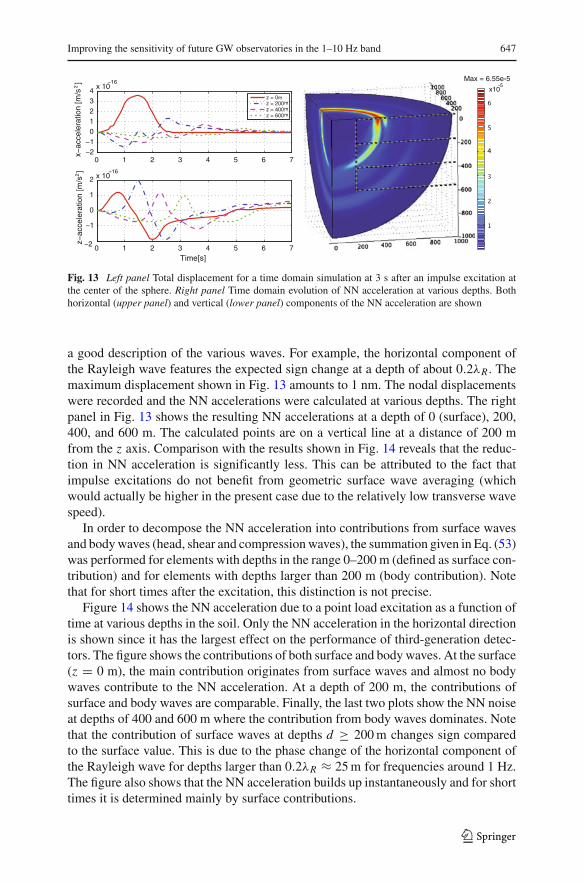
Fig. 13 Left panel Total displacement for a time domain simulation at 3 s after an impulse excitation atthe center of the sphere. Right panel Time domain evolution of NN acceleration at various depths. Bothhorizontal (upper panel) and vertical (lower panel) components of the NN acceleration are shown

a good description of the various waves. For example, the horizontal component ofthe Rayleigh wave features the expected sign change at a depth of about 0.2λR . Themaximum displacement shown in Fig. 13 amounts to 1 nm. The nodal displacementswere recorded and the NN accelerations were calculated at various depths. The rightpanel in Fig. 13 shows the resulting NN accelerations at a depth of 0 (surface), 200,400, and 600 m. The calculated points are on a vertical line at a distance of 200 mfrom the z axis. Comparison with the results shown in Fig. 14 reveals that the reduc-tion in NN acceleration is significantly less. This can be attributed to the fact thatimpulse excitations do not benefit from geometric surface wave averaging (whichwould actually be higher in the present case due to the relatively low transverse wavespeed).

In order to decompose the NN acceleration into contributions from surface wavesand body waves (head, shear and compression waves), the summation given in Eq. (53)was performed for elements with depths in the range 0–200 m (defined as surface con-tribution) and for elements with depths larger than 200 m (body contribution). Notethat for short times after the excitation, this distinction is not precise.

Figure 14 shows the NN acceleration due to a point load excitation as a function oftime at various depths in the soil. Only the NN acceleration in the horizontal directionis shown since it has the largest effect on the performance of third-generation detec-tors. The figure shows the contributions of both surface and body waves. At the surface(z = 0 m), the main contribution originates from surface waves and almost no bodywaves contribute to the NN acceleration. At a depth of 200 m, the contributions ofsurface and body waves are comparable. Finally, the last two plots show the NN noiseat depths of 400 and 600 m where the contribution from body waves dominates. Notethat the contribution of surface waves at depths d ≥ 200 m changes sign comparedto the surface value. This is due to the phase change of the horizontal component ofthe Rayleigh wave for depths larger than 0.2λR ≈ 25 m for frequencies around 1 Hz.The figure also shows that the NN acceleration builds up instantaneously and for shorttimes it is determined mainly by surface contributions.

123


0 2 4 6−2

−1

0

1

2

3

4x 10

−16 z=0 m

Acc

eler

atio

n [m

/s2 ]

0 2 4 6−3

−2

−1

0

1

2

3x 10

−16 z=200 m

0 2 4 6−1

−0.5

0

0.5

1x 10

−16 z=400 m

Acc

eler

atio

n [m

/s2 ]

Time [s]0 2 4 6

−4

−2

0

2

4x 10

−17 z=600 m

Time [s]

SurfaceBulkTotal

Fig. 14 Time domain horizontal NN acceleration response due to point load excitation at the origin of thehalf-sphere shown in Fig. 13. Top left NN acceleration at the surface, top right at 200 m depth, bottom leftat 400 m depth, bottom right at 600 m depth. The total NN acceleration and the contributions from surfaceand body waves are shown

4 Characterizing seismic noise at Homestake mine

Homestake mine was chosen by the NSF to host the Deep Underground Scienceand Engineering Laboratory (DUSEL). Efforts are under way to develop plans for theDUSEL facility and its initial suite of experiments on astroparticle experiments, whichrequire the low cosmic-ray background, biology, geology and seismology.

Homestake mine also provides a unique low gravitational background environment.The reduced seismic motion, the protection from variable weather, and the controlledlevel of human activity make the Homestake mine an ideal site for sensitive mechanicalmeasurements. The Homestake mine includes about 600 km of tunnels, allowing us toprobe correlations and propagation of seismic waves over kilometer-scale horizontaldistances. Due to the ongoing dewatering of the mine, it is currently possible to accesslevels down to 1,480 m. We have started to develop an array of seismic stations at theHomestake mine (see Figs. 15, 16), and currently have five operational stations: at 90,240, 610 and 1,250 m.

Each station operates at least one high-sensitivity broadband seismometer. Weinstrumented them with either the Streckheisen STS-2 and the Nanometrics T240low frequency seismometers (depending on availability), which are the best availableand have similar performance in the frequency band of interest, between 5–8 mHz and10–30 Hz. The instruments are placed onto horizontal granite tiles glued to a concreteslab that is well-connected to the bedrock. This arrangement was found to providegood contact with the rock and to minimize the effects of uneven surfaces. In addition

123


Fig. 15 Map of the levels with seismometer stations whose construction is completed. Two stations atthe 4,100 ft level and one at the 2,000 ft level are not yet operative. their seismometers are expected to beinstalled at those stations in September 2009

Fig. 16 Photos of the existing stations at the Homestake mine. From left to right instrument hut, seismom-eters, PCB operating environment monitors, and computer hut

to the seismometer, each station also operates a number of instruments to monitor theenvironment: thermometers, magnetometers, hygrometers, barometers, microphonesetc.

The instruments are isolated from the local acoustic disturbances and air-flow bynested huts made of rigid polyisocyanurate foam (at least two levels). They are read-out locally, using a standard PC with a National Instruments PCI-6289 digitizer card,located in a separate hut ∼10 m away. The computer is connected to the networkusing a fiber optic cable. This link is used both to transfer the data to the surface,and to synchronize the data acquisition at different locations. Timing is important inour studies, because they are focused on propagation and scattering of waves, as wellas measurement of propagation speed. Our current synchronization (at the level of0.2 ms) is based on NTP protocols, and is presently sufficient for our frequency bandof interest (0.1–10 Hz). A separate fiber link will be used to provide sub-microsecondtiming precision [21]. With the current data acquisition system the acquired data islimited below 1 Hz, this constraint is being removed.

The preliminary data acquired by the existing stations is already informative. Thevertical spectral displacement amplitude can be seen in Fig. 2, and apparently themine environment is seismically quiet. As shown in Fig. 17 (top), the environment ofthe mine is remarkably stable. Figure 18 shows that our near-surface station observes

123


Fig. 17 Preliminary data from Homestake. Top temperature stability of the 610 m station is remarkableover the 12-day period. Bottom spectral coherence of vertical displacement between stations at 610 and1,250 m depth is close to 1 below 0.1 Hz. The distance between the two stations is 1 km

a number of local disturbances (in the 0.2–1 Hz band) which are not present at thedeeper location, illustrating one reason why underground locations are preferred forgravitational-wave detectors. However, for a more detailed understanding of the seis-mic noise and its correlation length as a function of depth and position, three sta-tions are not sufficient—a more detailed network of stations is required. We expectto increase the array size to 8 stations (see Fig. 15) by the end of September 2009:with a sub-array of three at 1,250 and 610 m each, complementing the existing sta-tions at 240 and 90 m. Further expansions of the array are planned for the future.We expect that this array will begin to provide a more detailed understanding ofthe seismic noise underground. The data from this array will be used as an input tofinite-element models of the underground gravitational field, which will then producean estimate of the gravity gradient noise underground. The experiment will char-acterize the local site, and will provide a benchmark on how to characterize other

123


Fig. 18 Time-frequency maps of the seismic noise spectra at 90 m (left) and 610 m (right) indicate a largenumber of transient disturbances at 90 m at 0.2–1 Hz (likely due to local/surface disturbances). The 90 mdata below 0.1 Hz is known to be unreliable

perspective sites, as well as studying the measurement techniques necessary for NNsubtraction.

5 Seismic attenuation

The basic concept for seismic attenuation will likely be based on variations of theVirgo SuperAttenuators (SA) [22], which produce seismic attenuation in the Virgo-LIGO band and below [23]. Lower frequency attenuation will require longer chains,which practically eliminate the GEO-AdLIGO option of parallel attenuation chainsfor test mass controls, in favor of the branched topology of Virgo’s recoil masses. Theadaptation of seismic attenuation to cryogenic systems, if this option will be consid-ered, has been studied with the proposed LCGT detector in mind [24], and solved witha parallel attenuation chain isolating the chiller’s mechanical noise.

Producing seismic isolation for lower frequencies than in Virgo is a tough prob-lem and will introduce a whole host of new issues. The observed low-frequency extranoise in the superattenuator’s inverted pendula (IP) has shown a hint of the problemsto come. Seismic attenuation is based on harmonic oscillators, relying on materialelasticity (springs and flexures). Hysteresis and random motion observed in the VirgoIP, and later in the tilt hysteresis of masses suspended with metal wires, have drawnthe attention to the fact that at low frequencies the Young’s modulus of ordinary springmaterials are far from ideal and stable. New studies, as well as review of many, scat-tered, older observations, have shown evidence of time-dependent deviations from theHooke law below 1 Hz.

The evidence points towards a phase transition from dissipation dominated bymovement of individual dislocations, resulting in viscous-like behavior, to collec-tive dislocation activities, in a Self Organized Criticality state, resulting in avalanchedominated dissipation, spontaneous equilibrium point changes, and sudden tempo-rary drops of the Young’s modulus [25,26]. This anomalous behavior was observedto reduce the effectiveness of harmonic oscillators as vibration filters [27]. Becauseof this, the transfer function of a low frequency mechanical filter stage are observedto changes from an f −2 roll off to a much less effective f −1 roll off. If the problem

123


was limited to the reduction from f −2 to a f −1, it could be solved with brute force,by doubling the number of the filters in an attenuation chain.

But this effect can generate unexpected noises. At low frequency equilibrium pointrandom walk (due to dislocation distribution drifts), spontaneous collapse (due tosudden, although temporary, reduction of the Young’s modulus during dislocationre-arrangement) and large hysteresis, may produce fractal noise and vastly complicatethe problem of designing seismic attenuation systems at lower frequencies. Linearcontrols would have to be abandoned, in favor of more advanced schemes. Furtherstudies are needed to understand this issue.

The problem is not hopeless though, it is not clear if there will be excess noisein seismic attenuators after sufficiently long settling time and in sufficiently stablethermal conditions. Torsion pendula show excess noise for hours after large perturba-tions, but were observed to reach their expected thermal noise limited behavior aftersufficient time [28].

Additionally, as most of the identified problems appear to be connected to disloca-tion movement in polycrystalline metals, springs can be manufactured with alternativematerials, like glassy metals that having no crystals have no dislocations, or ceramicmaterials (for example tungsten carbide) that having polar bonds only have frozendislocations. Impeding or avoiding dislocation mobility is expected to restore the f −2

transfer function of the filters, and more importantly remove the additional sources ofinternal noise.

The use of dislocation-free or frozen-dislocation materials may inevitably intro-duce some level of fragility (this is the case of ceramic materials, but not of glassymetals) and complicate the engineering, but it does not seem to pose insurmountabletechnical problems. Confident that these engineering problems can be solved in thenear future (just as the introduction of Maraging steel has made the Virgo cantileversprings possible) we can try to have a peek to possible seismic attenuation schemesfor lower frequencies.

The 7-m tall Virgo superattenuators provide attenuation that crosses into the mirrorthermal noise level at 7–8 Hz, quite sufficient for a GWID sensitive above 10 Hz.A naively equivalent superattenuator, designed to allow GW detection starting from1 Hz, would require pendula 100 times longer and be more than 500 m tall. Suchtall pendula would be unthinkable on the surface but not too difficult to realize under-ground, where the longer suspension wires could be housed in low-diameter bore holesand the filters housed in small caverns dug at different heights along the bore hole.Fortunately it is not necessary to build such a tall seismic attenuator.

Labeling with T Hi the horizontal displacement transfer function from the top sus-

pension point to the mass of the i-th pendulum, numerated top to the bottom, we canwrite

⎛⎜⎜⎜⎜⎜⎜⎝

T H1

T H2......

T HN

⎞⎟⎟⎟⎟⎟⎟⎠

=

⎛⎜⎜⎜⎜⎜⎜⎝

d1 −k2−k2 d2 −k3

−k3. . .

. . .

. . .. . . −kN

−kN dN

⎞⎟⎟⎟⎟⎟⎟⎠

−1⎛⎜⎜⎜⎜⎜⎜⎝

k10......

0

⎞⎟⎟⎟⎟⎟⎟⎠

(54)

123


where the coefficient are defined as

ki = τi

�i= g

�i

N∑k=i

mk and di = ki + (1 − δi N ) ki+1 − miω2 (55)

and τi is the tension of the i th pendulum, �i its length, mi its mass.In order to find the attenuation of the last stage it is enough to determine the N , 1

element of the inverse of the tridiagonal, symmetric matrix [29] obtaining for thetop-bottom displacement transfer function

T HN =

N∏p=1

kp

Cbp

(56)

where Cbp is the pth convergent of the backward continued fraction associated with

the tridiagonal matrix in Eq. (54),

Cbp = dp − k2

p

dp−1 − k2p−1

. . .

d2 − k22

d1

(57)

In the higher frequency region Cbp � dp � −m pω

2 and we get the expected powerlaw behavior

T HN � (−1)N 1

f 2N

N∏p=1

⎡⎣ g

(2π)2 �p

N∑k=p

mk

m p

⎤⎦ (58)

In Virgo the horizontal attenuation chain was designed with seven 1 m tall pendula,then reduced to 5 in the practical implementation, each with the same mass and with

fpendulum = 1

2π

√g

�= 5 × 10−1 Hz (59)

and this gives (in the 7 stages case)

T HN � −5040

(fpendulum

f

)14

(60)

where the large numerical factor is connected to the fact that each pendulum in thechain has a different tension. At 10 Hz we get

∣∣T HN

∣∣ � 3 × 10−15. Similar consid-erations can be done for the vertical top-bottom transfer function T V

N , with a maindifference. Here the low frequency spring effect is obtained with a Magnetic Anti

123


Fig. 19 Horizontal attenuationperformances of asuperattenuator chain at 1 Hz(vertical axis) as a function ofthe total length of the chain(horizontal axis, in meters) forseveral number of stages. Theparameters of each stage are thesame. In order of increasingthickness the plot correspond ton = 2, 3, 4, 5, 6, 7, 8, 9 stages

10 1005020 2003015 15070Chain length (m)

10 12

10 11

10 10

10 9

10 8

10 7

10 6

10 5

10 4

10 3

10 2

10 1

1

10

100

Atte

nuat

ion

Spring (MAS) filter, described by spring constants χi that can be supposed to be equaland

T VN � (−1)N 1

f 2N

N∏p=1

χp

(2π)2 m p= (−1)N

(fM AS

f

)2N

(61)

without the large multiplicative factor. Note that fM AS = 3 × 10−1 Hz. This allowsthe superattenuator to obtain the required attenuation with a relatively small numberof filters.

The lower level of seismic noise underground requires less attenuation, thus requir-ing 4, or maybe even as little as 3 attenuation filter stages below the initial invertedpendulum, assuming the use of the new GAS filters, which provide almost doubleattenuation (80 dB/unit instead of 40 dB/unit) than the older MAS filters. If the verti-cal height was still a problem one can reduce to half the overall length of the attenuationchain, without losing performance, by doubling the number of stages, within each sec-tion. A two stage chain delivering 10−5 attenuation at 1 Hz is 200 m tall (see Fig. 19,red line). It can be replaced by a three stage chain with the same performances 70 mtall (Fig. 19, orange line), or by a four stage one 40 m tall (Fig. 19, light green line).

Attenuation chains shorter than 200 m can be designed with present technologies.Completely new developments would be required to design shorter ones. The IP isa compact horizontal attenuator. Unfortunately, while it is easy to chain normal pen-dula, chaining more than one stage of IPs results in instability. Shortened, but lowfrequency pendula may be possible by applying horizontal magnetic anti-springs tonormal pendula.

123


6 Conclusions

The need to reduce both the seismic and gravity gradient noise can be fulfilled by anunderground site. Low seismic activity and uniformity of the soil plays a dominantrole in the site identification process. As a next step the effectiveness of NN subtractionschemes will be studied in detail. We expect that a synergy between analytical work,numerical modelizations and seismic measurements will improve in the near futureour understanding of the problem, allowing us to obtain more accurate and trustablepredictions. This will be important in order to make a good choice for the sites of thirdgeneration interferometers.

A vigorous R&D effort to improve the sensitivity of inexpensive borehole typedetectors to rock motion and density will be necessary to fulfill the target of bringingthe sensitivity of underground GW observatories all the way down to 1 Hz.

Alternative to the underground solution involves the possibility of finding a quietenough place on the surface, or a space based detector. The first option does not seemsfeasible up to our knowledge, but a search effort in this direction is surely important.

Concerning the space option, it will be hardly less expensive. A single space-bornedetector cannot compete with an underground detector at frequencies where both canachieve similar sensitivity.

We are not proposing in any way that something like a BBO [30] can be built onEarth. Our NN discussion is really relevant for a one-on-one comparison, not for com-paring space-borne arrays with arrays on Earth. Space-borne arrays obviously willhave a great advantage at low frequencies.

Acknowledgments We are grateful to Dr. Rudolf Widmer-Schnidrig from the University of Stuttgart forpermission to use Fig. (3). This work is part of the research programme of the Foundation for FundamentalResearch on Matter (FOM), which is financially supported by the Netherlands Organization for ScientificResearch (NWO). Funding and support of this study is also provided by The National Science Foundationthrough the LIGO cooperative agreement and the Minnesota U. grant.

Open Access This article is distributed under the terms of the Creative Commons Attribution Noncom-mercial License which permits any noncommercial use, distribution, and reproduction in any medium,provided the original author(s) and source are credited.

References

1. Hild, S., Chelkowski, S., Freise, A.: Pushing towards the ET sensitivity using ‘conventional’technology. arXiv:0810.0604v2 (2008)

2. Hild, S., et al.: A xylophone configuration for a third generation gravitational wave detector (2009),arXiv:0906.2655

3. Advanced LIGO anticipated sensitivity curves. LIGO-T0900288-v2, https://dcc.ligo.org/cgi-bin/private/DocDB/ShowDocument?docid=2974

4. Saulson, P.: Terrestrial gravitational noise on a gravitational wave antenna. Phys. Rev. D 30, 732 (1984)5. Hughes, S.A., Thorne, K.S.: Seismic gravity-gradient noise in interferometric gravitational-wave detec-

tors. Phys. Rev. D 58, 122002 (1998)6. Beccaria, M., et al.: Relevance of Newtonian seismic noise for the VIRGO interferometer sensitiv-

ity. Class. Quantum Grav. 15, 3339 (1998)7. Creighton, T.: Tumbleweeds and airborne gravitational noise sources for LIGO. Class. Quantum

Grav. 25, 125011 (2008)

123

https://dcc.ligo.org/cgi-bin/private/DocDB/ShowDocument?docid=2974



8. Cafaro, C., Ali, S.A.: Analytical estimate of atmospheric Newtonian noise generated by acoustic andturbulent phenomena in laser-interferometric gravitational waves detectors. arXiv:0906.4844 [gr-qc]

9. Hough, S.E., et al.: Ambient noise and weak-motion excitation of sediment resonances: results fromthe Tiber Valley, Italy. Bull. Seism. Soc. Am. 82, 1186 (1992)

10. Bour, M., et al.: On the use of microtremor recordings in seismic microzonation. Soil Dyn. Earth.Eng. 17, 465 (1998)

11. Noble, J.A., Harder, J.O.: Stratigraphy and metamorphism in a part of the Northern Black Hills andthe Homestake mine, Lead, South Dakota. Bull. Geol. Soc. Am. 50, 941 (1948)

12. Einstein Telescope WG1 report: selection criteria for ET candidate sites (2009)13. Grote, H.: Seismic Data from the Black Forest Underground Station and Experience from Kamioka,

ET, WP1 meeting, Gran Sasso, (February 2009)14. Berger, et al.: Ambient earth noise: a survey of the global seismographic network. JGR 109, B11307

(2004)15. Peterson, J.: Observations and modeling of seismic background noise. US Department of Interior

Geological Survey, Open-file report 93–322 (1993)16. Caticha, A., Preuss, R.: Maximum entropy and bayesian data analysis: entropic priors. Phys. Rev. E

70, 04612717. Cella, G.: Off line subtraction of seismic Newtonian noise. In: Casciaro, B., Fortunato, D., Francaviglia,

M., Masiello, A. Recent Developments in General Relativity, Springer, Heidelberg (2000)18. Saulson, P.R.: Fundamentals of Interferometric Gravitational Wave Detectors. World Scientific,

Singapore (1997)19. Thorne, K.S., Winstein, C.J.: Human gravity-gradient noise in interferometric gravitational-wave detec-

tors. Phys. Rev. D 60, 082001 (1999)20. Woods, R.D.: Screening the surface waves in soils. In: Proceedings of ASCE 94 SM4, 951–97921. Bartos, R., et al.: Timing system document map advanced LIGO, LIGO-090003, https://dcc.ligo.org/

cgi-bin/private/DocDB/ShowDocument?docid=48322. Braccini, S., et al.: Measurement of the seismic attenuation performance of the VIRGO Superattenu-

ator. Astropart. Phys. 23, 557–565 (2005)23. Braccini, S., et al.: Superattenuator seismic isolation measurement by Virgo interferometer: a com-

parison with the future generation antenna requirements. ET-025-09 (Technical report of EinsteinTelescope FP7 Design Study). Submitted to Astropart. Phys

24. Ohashi, M.: Status of LCGT and CLIO. J. Phys. Conf. Ser. 120, 032008 (2008)25. Di Cintio, A., Marchesoni, F., Ascione, M., Bhawal, A., De Salvo, R.: Dislocation movement and

hysteresis in Maraging blades. LIGO-P090092826. Di Cintio, A.: Astrophysics issues and low frequency mechanical noise for third generation gravita-

tional waves detectors. Master Thesis, LIGO -P090007627. Stochino, A., et al.: Improvement of the seismic noise attenuation performance of the Monolithic

Geometric Anti-Spring filters for gravitational wave interferometric detectors. Nucl. Instr. Meth. Phys.Res. A 580(3), 1559–1564 (2007)

28. Schlamminger, S., Gurlach, J.: Private communication (2009)29. Kılıç, E.: Explicit formula for the inverse of a tridiagonal matrix by backward continued fractions. Appl

Math Comput 197, 345–357 (2008)30. Phinney, S., Bender, P., Buchman, S., Byer, R., Cornish, N., Fritschel, P., Folkner, W., Merkowitz, S.,

Danzmann, K., DiFiore, L., Kawamura, S., Schutz, B., Vecchio, A., Vitale, S.: The Big Bang Observer,BBO Proposal

123



Improving the sensitivity of future GW observatories in the 1â€“10

Documents

Transcript of Improving the sensitivity of future GW observatories in the 1â€“10