IMPROVING THE COMPUTATIONAL EFFICIENCY OF TRAINING AND ...

IMPROVING THE COMPUTATIONAL

EFFICIENCY OF TRAINING AND APPLICATION

OF NEURAL LANGUAGE MODELS FOR

AUTOMATIC SPEECH RECOGNITION

by

Hainan Xu

A dissertation submitted to The Johns Hopkins University

in conformity with the requirements for the degree of

Doctor of Philosophy

Baltimore, Maryland

October 2020

© 2020 by Hainan Xu

All rights reserved

Abstract

A language model is a vital component of automatic speech recognition sys-

tems. In recent years, advancements in neural network technologies have

brought vast improvement in various machine learning tasks, including lan-

guage modeling. However, compared to the conventional backoff n-gram

models, neural networks require much greater computation power and cannot

completely replace the conventional methods.

In this work, we examine the pipeline of a typical hybrid speech recognition

system. In a hybrid speech recognition system, the acoustic and language

models are trained separately and used in conjunction. We propose ways to

speed up the computation induced by the language model in various com-

ponents. In the context of neural-network language modeling, we propose

a new loss function that modifies the standard cross-entropy loss that trains

the neural network to self-normalize, which we call a linear loss. The linear

loss significantly reduces inference-time computation and allows us to use an

importance-sampling based method in computing an unbiased estimator of

the loss function during neural network training.

We conduct extensive experiments comparing the linear loss and several

ii

commonly used self-normalizing loss functions and show linear loss’s su-

periority. We also show that we can initialize with a well-trained language

model trained with the cross-entropy loss and convert it into a self-normalizing

linear loss system with minimal training. The trained system preserves the

performance and also achieves the self-normalizing capability.

We refine the sampling procedure for commonly used sampling-based ap-

proaches. We propose using a sampling-without-replacement scheme, which

improves the model performance and allows a more efficient algorithm to

be used to minimize the sampling overhead. We propose a speed-up of the

algorithm that significantly reduces the sampling run-time while not affecting

performance. We demonstrate that using the sampling-without-replacement

scheme consistently outperforms traditional sampling-with-replacement meth-

ods across multiple training loss functions for language models.

We also experiment with changing the sampling distribution for importance-

sampling by utilizing longer histories. For batched training, we propose a

method to generate the sampling distribution by averaging the n-gram distri-

butions of the whole batch. Experiments show that including longer histories

for sampling can help improve the rate of convergence and enhance the trained

model’s performance. To reduce the computational overhead with sampling

from higher-order n-grams, we propose a 2-stage sampling algorithm that

only adds a small overhead compared to the commonly used unigram-based

sampling schemes.

When applying a trained neural-network for lattice-rescoring for ASR, we

iii

propose a pruning algorithm that runs much faster than the standard algorithm

and improves ASR performances.

The methods proposed in this dissertation will make the application of neu-

ral language models in speech recognition significantly more computationally

efficient. This allows researchers to apply larger and more sophisticated net-

works in their research and enable companies to provide better speech-based

service to customers. Some of the methods proposed in this dissertation are

not limited to neural language modeling and may facilitate neural network

research in other fields.

Primary reader: Daniel Povey

Secondary reader: Sanjeev Khudanpur

Third reader: Philipp Koehn

iv

Acknowledgments

First of all, I would want to thank Dr. Daniel Povey, my primary advisor, for

his close guidance in the past six years of my Ph.D. program. Also, for his

relentless efforts in protecting the servers of Center for Language and Speech

Processing at Johns Hopkins University. What happened to Dan that caused

his firing from the university was unfair. While I hope things could be different,

I am glad that he found employment opportunities with Xiaomi China. I am

glad that now Dan can work with some of the best speech researchers globally

and have complete freedom to improve speech recognition and help build

products that reach hundreds of millions of users worldwide.

I also want to thank Prof. Sanjeev Khudanpur, my advisor, for his guidance

in my research projects and for sharing his life wisdom in our frequent conver-

sations. Sanjeev showed me how to be a better researcher and taught me how

to be a better human being. I also owe a lot of gratitude to Sanjeev for doing an

impeccable job maintaining my funding over the past years.

I am also grateful to Prof. Kai Yu for first taking me to the beautiful world

of speech research; to Prof. Philipp Koehn, Prof. Shinji Watanabe, Dr. Guoguo

Chen, for their guidance on research projects at JHU. I also owe much gratitude

v

to Dr. Bhuvana Ramabhadran, my current manager at Google, for her guidance

in my work and also being supportive while I prepared for my defense and

wrote my thesis while working with her.

I also want to express my utmost gratitude to Dr. Leslie Leathers, Dr. Scott

Spier, Dr. Michael Lint, and Dr. Alex Szablya, who at different times were my

therapist. Working on a Ph.D. takes many tolls on a person’s mental health,

and I would not have been able to make it if it were not for the counseling

sessions I have had with you.

I also want to thank Dr. Jordan Peterson. I know Dr. Peterson is a contro-

versial figure, and I cannot entirely agree with everything he said. But I benefit

immensely from his advice to “compare yourself to who you were yesterday,

not to who someone else is today”, as well as the most straightforward advice

to just "clean your room before you criticize the world”. Personal development

is an endless pursuit, and I am glad that I have taken Dr. Peterson’s advice to

do my best to work on myself, and I will try to keep doing that going forward.

vi

Table of Contents

Abstract ii

Acknowledgments v

Table of Contents vii

List of Tables xii

List of Figures xv

1 Introduction 1

1.1 The Speech Recognition Problem . . . . . . . . . . . . . . . . . . 1

1.2 Mathematical Analysis of Speech Recognition . . . . . . . . . . 5

1.3 Language Models . . . . . . . . . . . . . . . . . . . . . . . . . . . 6

1.3.1 n-gram Language Models . . . . . . . . . . . . . . . . . . 8

1.3.2 Neural-network Language Models . . . . . . . . . . . . . 10

1.4 Application of Language Models in ASR . . . . . . . . . . . . . . 14

1.4.1 2-pass Method . . . . . . . . . . . . . . . . . . . . . . . . 15

1.4.1.1 n-best Rescoring . . . . . . . . . . . . . . . . . . 15

1.4.1.2 Lattice Rescoring . . . . . . . . . . . . . . . . . . 16

vii

1.5 Evaluation of Language Models in ASR . . . . . . . . . . . . . . 17

1.6 Limitations of RNNLMs in ASR . . . . . . . . . . . . . . . . . . . 19

1.6.1 Training . . . . . . . . . . . . . . . . . . . . . . . . . . . . 19

1.6.2 Inference . . . . . . . . . . . . . . . . . . . . . . . . . . . . 20

1.6.3 Rescoring algorithms . . . . . . . . . . . . . . . . . . . . . 21

1.6.4 Contribution of this Dissertation . . . . . . . . . . . . . . 22

I Improving the Computational Efficiency of RNNLMs 25

2 Linear Loss: an Alternative to Cross-entropy Loss 27

2.1 Cross-Entropy Loss Function . . . . . . . . . . . . . . . . . . . . 27

2.1.1 Log-softmax Function . . . . . . . . . . . . . . . . . . . . 28

2.1.2 Cross-entropy Implementation . . . . . . . . . . . . . . . 29

2.2 Linear Loss . . . . . . . . . . . . . . . . . . . . . . . . . . . . . . . 31

2.3 Experiments . . . . . . . . . . . . . . . . . . . . . . . . . . . . . . 33

2.3.1 Datasets . . . . . . . . . . . . . . . . . . . . . . . . . . . . 34

2.3.2 Language Modeling Performance . . . . . . . . . . . . . 35

2.3.3 Initializing with Cross-entropy Systems . . . . . . . . . . 38

2.3.4 Hybrid Speech Recognition Performance . . . . . . . . . 39

2.3.4.1 Speech Recognition Performance . . . . . . . . 40

2.3.4.2 Speech Recognition Performance - One Epoch

Training . . . . . . . . . . . . . . . . . . . . . . . 43

2.3.4.3 Speed of RNNLM Computation . . . . . . . . . 44

2.3.5 End-to-end Speech Recognition Performance . . . . . . . 45

2.4 Chapter Summary . . . . . . . . . . . . . . . . . . . . . . . . . . . 46

viii

3 RNNLM Training with Sampling 49

3.1 Importance-sampling . . . . . . . . . . . . . . . . . . . . . . . . . 50

3.2 RNNLM Training with Sampling-based Methods . . . . . . . . . 51

3.2.1 Importance-sampling for Cross-entropy Training . . . . 51

3.2.2 Importance-sampling for Linear Loss Training . . . . . . 53

3.2.3 Sampling Distributions . . . . . . . . . . . . . . . . . . . 54

3.2.4 Noise-contrastive Estimation . . . . . . . . . . . . . . . . 56

3.3 Importance-sampling for Variance-Regularization . . . . . . . . 58

3.4 Chapter Summary . . . . . . . . . . . . . . . . . . . . . . . . . . . 59

4 Evaluation of Linear Loss 61

4.1 Comparison with Variance Regularization . . . . . . . . . . . . . 64

4.2 Comparison with Noise-contrastive Estimation . . . . . . . . . . 65

4.3 Comparison with Sampled Softmax . . . . . . . . . . . . . . . . 67

4.4 Comparison with Sampled Variance Regularization . . . . . . . 69

4.5 Chapter Summary . . . . . . . . . . . . . . . . . . . . . . . . . . . 71

5 Impact of Sampling Algorithm on Language Model Training 73

5.1 Sampling with Replacement . . . . . . . . . . . . . . . . . . . . . 74

5.2 Sampling without Replacement . . . . . . . . . . . . . . . . . . . 76

5.3 Sampling without Replacement: Algorithm . . . . . . . . . . . . 78

5.3.1 An Obvious (and Wrong) Approach . . . . . . . . . . . . 78

5.3.2 Reservoir Sampling Algorithm . . . . . . . . . . . . . . . 80

5.3.3 2-stage Reservoir Sampling Algorithm . . . . . . . . . . . 82

5.3.4 Systematic Sampling Algorithm . . . . . . . . . . . . . . 85

ix

5.3.5 2-stage systematic sampling . . . . . . . . . . . . . . . . . 87

5.4 Computing Inclusion Probabilities . . . . . . . . . . . . . . . . . 88

5.5 Evaluation of Different Sampling Methods . . . . . . . . . . . . 91

5.6 Language Modeling Experiments . . . . . . . . . . . . . . . . . . 93

5.6.1 The Impact of Replacement . . . . . . . . . . . . . . . . . 94

5.7 Chapter Summary . . . . . . . . . . . . . . . . . . . . . . . . . . . 95

6 Batch Training and Sampling from Longer Histories 97

6.1 Average n-gram Distribution in a Batch . . . . . . . . . . . . . . 99

6.2 Sampling with Longer Histories . . . . . . . . . . . . . . . . . . . 100

6.3 Experiments . . . . . . . . . . . . . . . . . . . . . . . . . . . . . . 105

6.4 Chapter Summary . . . . . . . . . . . . . . . . . . . . . . . . . . . 107

II Improving the Computational Efficiency of RNNLM Lat-

tice Rescoring 109

7 Lattice Rescoring in the FST Framework 111

7.1 Finite-state Automaton . . . . . . . . . . . . . . . . . . . . . . . . 112

7.2 Finite-state Transducer . . . . . . . . . . . . . . . . . . . . . . . . 115

7.3 FST Composition . . . . . . . . . . . . . . . . . . . . . . . . . . . 116

7.4 FST Representation of Lattices . . . . . . . . . . . . . . . . . . . . 118

7.5 Lattice-rescoring with FST Composition . . . . . . . . . . . . . . 120

7.5.1 Exact Lattice Rescoring . . . . . . . . . . . . . . . . . . . 125

7.5.2 Lattice Rescoring with n-gram Approximations . . . . . 127

7.6 Chapter Summary . . . . . . . . . . . . . . . . . . . . . . . . . . . 132

x

8 Pruned Lattice Rescoring 133

8.1 Pruned composition . . . . . . . . . . . . . . . . . . . . . . . . . 134

8.2 Heuristics . . . . . . . . . . . . . . . . . . . . . . . . . . . . . . . 136

8.2.1 Assumption . . . . . . . . . . . . . . . . . . . . . . . . . . 137

8.2.2 Background: α and β Scores . . . . . . . . . . . . . . . . . 138

8.2.3 Heuristic . . . . . . . . . . . . . . . . . . . . . . . . . . . . 140

8.3 Applying the Heuristics in Composition . . . . . . . . . . . . . . 143

8.3.1 Lazy Updates of Forward/Backward Scores . . . . . . . 143

8.3.2 Initial Computation . . . . . . . . . . . . . . . . . . . . . 145

8.4 Experiments . . . . . . . . . . . . . . . . . . . . . . . . . . . . . . 146

8.4.1 Rescoring Speed and Output Lattice Size . . . . . . . . . 146

8.4.2 WER performances . . . . . . . . . . . . . . . . . . . . . . 150

8.5 Chapter Summary . . . . . . . . . . . . . . . . . . . . . . . . . . . 151

9 Conclusion 153

Vita 171

xi

List of Tables

2.1 Model Stats on AMI Corpus Showing Perplexity, Mean, Variance

and Ratio between Standard Deviation and Mean for the Nor-

malization Term for the Output of Models Trained with Different

Loss Functions. . . . . . . . . . . . . . . . . . . . . . . . . . . . . 36

2.2 Perplexity of Models Trained with Different Loss Functions on

WSJ Corpus . . . . . . . . . . . . . . . . . . . . . . . . . . . . . . 37

2.3 Model Stats on WSJ Corpus Showing Perplexity, Mean, Vari-

ance and Ratio between Standard Deviation and Mean for the

Normalization Term for the Output of Models Trained with Dif-

ferent Loss Functions. The Linear Loss System is Trained for

One Epoch after Initializing with a Well-trained Cross-entropy

System. . . . . . . . . . . . . . . . . . . . . . . . . . . . . . . . . . 39

2.4 WER of AMI-SDM Corpus When Rescored by Different RNNLMs. 40

2.5 WER of WSJ Corpus When Rescored by Different RNNLMs. . . 41

2.6 WER in AMI-SDM When Rescored by Different RNNLMs with

Different Normalization Schemes. . . . . . . . . . . . . . . . . . 42

2.7 WER in WSJ When Rescored by Different RNNLMs with Differ-

ent Normalization Schemes. . . . . . . . . . . . . . . . . . . . . . 43

xii

2.8 WER in WSJ of Cross-entropy and Linear-loss Systems. The

Linear loss System is Trained for One Epoch after Initializing

with a Well-trained Cross-entropy Model. . . . . . . . . . . . . . 43

2.9 Time Spent Rescoring 10000 Randomly Selected Sentences from

n-best Lists with Different RNNLMs on AMI Corpus. For Linear

loss RNNLM, Normalization is Not Performed on the Output. . 44

2.10 Time Spent Rescoring 10000 Randomly Selected Sentences from

n-best Lists with Different RNNLMs on WSJ Corpus. For Linear

loss RNNLM, Normalization is Not Performed on the Output. . 45

2.11 WER of Shallow Fusion with Different LMs for E2E ASR on WSJ

Corpus. Normalization is not Performed on the Output of the

Linear Model. . . . . . . . . . . . . . . . . . . . . . . . . . . . . . 46

4.1 Model Stats on AMI Corpus Showing Perplexity, Mean, Variance

and Ratio between Standard Deviation and Mean for the Nor-

malization Term for the Output of Models Trained with Different

Loss Functions. . . . . . . . . . . . . . . . . . . . . . . . . . . . . 63

4.2 Comparisons of WER% on AMI-SDM Corpus, Linear Loss VS

Variance Regularization . . . . . . . . . . . . . . . . . . . . . . . 65

4.3 Mean and Variance of Unnormalized Outputs in AMI with

Sampling-based Training, Linear VS NCE, Sampling with Re-

placement . . . . . . . . . . . . . . . . . . . . . . . . . . . . . . . 66

4.4 Comparison of WER of RNNLMs Trained with Linear Loss VS

NCE . . . . . . . . . . . . . . . . . . . . . . . . . . . . . . . . . . . 67


Sampled Softmax . . . . . . . . . . . . . . . . . . . . . . . . . . . 68

xiii

4.6 Mean and Variance of Unnormalized Outputs in AMI with

Sampling-based Training, Sampled VR VS Linear, Sampling

with Replacement . . . . . . . . . . . . . . . . . . . . . . . . . . . 69


Sampled VR . . . . . . . . . . . . . . . . . . . . . . . . . . . . . . 70

5.1 Time (of t runs of n choose k in seconds) of Sampling from

Unigrams . . . . . . . . . . . . . . . . . . . . . . . . . . . . . . . . 92

5.2 Comparison between Different Sampling Methods . . . . . . . . 94

6.1 Effect of Sampling From Longer History in Switchboard . . . . 106

7.1 Statistics on Kaldi Generated Lattices for Different Datasets . . . 120

8.1 Speed (seconds) Comparison of Lattice-rescoring, AMI-DEV . . 149

8.2 Output Lattice-size Comparison of Lattice-rescoring, AMI-DEV 149

8.3 WER of Lattice-rescoring of Different RNNLMs in Different

Datasets . . . . . . . . . . . . . . . . . . . . . . . . . . . . . . . . 151

xiv

List of Figures

1.1 A Demonstration of a Simple RNNLM Working on Text Se-

quence "I am Spartacus". . . . . . . . . . . . . . . . . . . . . . . . 13

1.2 An Example of a Simple Word Lattice. . . . . . . . . . . . . . . . 16

2.1 Comparing -log(x) (blue) and 1 - x (red). . . . . . . . . . . . . . . 33

2.2 Comparison of Cross-entropy Loss to Number of Epochs for

Models Trained with Different Loss Functions. . . . . . . . . . . 38

5.1 Visual Aid to Help Understand the Systematic Sampling Algo-

rithm. . . . . . . . . . . . . . . . . . . . . . . . . . . . . . . . . . . 86

6.1 Changing group assignments for words when changing the

sampling distribution from unigrams to higher-order n-grams.

The group containing words w1, ..., w7 is divided into 4 groups

since w1 and w4 have higher-order n-gram probabilities. . . . . 104

6.2 Convergence Rate VS Sampling Distribution . . . . . . . . . . . 107

xv

7.1 Diagram depicting the author’s experience of working on a Ph.D.

It consists of three states and four directed arcs connecting one

state to another. This diagram does not satisfy the condition for

finite-state automata because it does not have a start state and a

final state. . . . . . . . . . . . . . . . . . . . . . . . . . . . . . . . 113

7.2 A finite-state automaton depicting the author’s experience of

working on PhD. It consists of five states, and 6 directed arcs

connecting one state to another. The start state is represented by

the double circle and the final state is represented by the triple

circle. . . . . . . . . . . . . . . . . . . . . . . . . . . . . . . . . . . 114

7.3 Copy of the Word Lattice Example First Shown in Figure 1.2 . . 119

7.4 A Real Lattice for SWBD-Eval2000 Data Generated by Kaldi,

Utterance ID: en_4156-A_030470-030672. The reference for the

utterance is, “well i am going to have mine in two more classes.”

The lattice has a start-state 0 at the left and a final state 48 at

the bottom right, with 127 arcs. The word labels on each arc is

shown, but we omit the weights. . . . . . . . . . . . . . . . . . . 121

7.5 Topology of lattice from Figure 7.3 if rescored by a bi-gram

model. Note this lattice is partial, and only shows the part that

is close to the start-state of the lattice. . . . . . . . . . . . . . . . . 123

7.6 Topology of lattice from Figure 7.3 if rescored by an RNNLM.

Note this lattice is partial, and only shows the part that is close

to the start-state of the lattice. . . . . . . . . . . . . . . . . . . . . 124

7.7 Examples of Lattices . . . . . . . . . . . . . . . . . . . . . . . . . 129

8.1 Average run-time (in seconds) of lattice-rescoring, AMI-DEV . . 147

xvi

en_4156-A_030470-030672

8.2 Average number of arcs per frame of rescored lattices, AMI-DEV 148

xvii

This page was left intentionally blank.

xviii

Chapter 1

Introduction

1.1 The Speech Recognition Problem

Speech is one of the, if not the most, natural way[s] for people to communicate

with each other and to convey information. In this information age, there is a lot

of demand for computers to “understand” human speech, and researchers have

been working for decades trying to solve this task. While the word “understand”

is hard to define, few would argue that to extract the text information from the

speech is a vital first step before any understanding is possible. This defines

the task of automatic speech recognition (ASR) [1], i.e., of designing a system that

can accurately transcribe a representation of audio (for example, waveform or

MP3 audio that we could play on a computer, or extracted acoustic features

including Mel-frequency cepstral coefficients [2] (MFCC) or Perceptual linear

predictive [3] (PLP), etc.) into text. While the ability to recognize speech

1

comes naturally to most humans, it is no easy task for machines. Although

researchers have come up with different speech processing models and made

significant progress in ASR [4, 5, 6] for the last five decades, speech recognition

remains a challenging problem, especially in noisy environments and/or with

spontaneous/accented speech.

The basic principles of solving the speech recognition problem have ex-

perienced many shifts in the past decades. In the earliest speech recognition

systems, researchers built a “template” for each word in the vocabulary and

used dynamic time warping [7] or similar methods for computing a “distance”

between the template word and audio input to be recognized. This method

works well for isolated word-recognition, e.g., recognizing single word com-

mands. However, suppose an input sequence has multiple words. In that case,

a separate stage of processing is needed to find boundaries between words

before the speech recognition model recognizes the word from each segment.

Overall, while there was progress, this class of methods did not make the

speech recognition technology applicable to real-life uses.

With the introduction of the Dragon System [8], Hidden Markov Models

(HMM) began their long success in the speech recognition community, up to

this day. At the same time, the problem of speech recognition also became

modular, where a typical system would comprise of several sub-components,

including an acoustic model, a lexicon, a language model, and a decoder. In

each of those components, researchers have worked on improving model per-

2

formance. For acoustic modeling, we have seen a shift from adopting Gaussian-

mixture Models (GMM), to sub-space GMM [9], to Deep neural network (DNN)

based models [10]; we have also seen different training schemes proposed,

including Maximum-likelihood Estimation (MLE) [11], Maximum A-Posteriori

Estimation (MAP) [12] and discriminative training objectives [13], including

Maximum Mutual Information (MMI) training [14] and Minimum Phone Error-

rate (MPE) training [15]. Some linguistic knowledge was also shown to help

improve ASR performance, especially in earlier times; for example, expert

knowledge of a phone set of a language was used in constructing questions for

building phonetic decision trees [16] in order to cluster acoustic model units.

Although gradually, the reliance on linguistic knowledge started to disappear.

Rumor has it that the great speech scientist Fred Jelinek has said, Every time I

fire a linguist, the performance of our speech recognition system goes up. Although

there is a certain level of exaggeration in this quote, it does reflect the real trend,

namely, that we are moving towards building a speech recognition system from

data alone without external knowledge about languages. Even the lexicon (a

pronunciation dictionary), which gives vital information on how words are

pronounced, is sometimes unnecessary for many languages. Researchers have

discovered that graphemic (letter-based) systems [17] can work surprisingly

well, not only for languages like Spanish, which has a simple spelling to pro-

nunciation mapping, but even for languages like English, whose spelling to

pronunciation mapping is quite complicated and lacks structure. The recent

3

success seen in end-to-end speech recognition further proves this trend.

Several techniques, including model adaptation [18] and model combina-

tion [19], are shown to be useful in improving ASR performance, either in their

generic forms or within the context of phonetic decision trees [20, 21]. With the

incorporation of phonetic decision trees to classify context-dependent phones

for generating modeling units, and the complexity of representing a phonetic

dictionary and a language model, there was a high bar for researchers to imple-

ment a correct decoder for large vocabulary continuous speech recognition (LVCSR).

Fortunately, those sub-components of ASR systems, in the last decade, have

been elegantly unified in the weight finite-state transducer (WFST) framework

[22, 23], which not only provides an elegant mathematical foundation of the

methods but also makes the system more efficient and the algorithms easier to

implement.

In the last ten years, as neural machine translation (NMT) models [24] have

gradually surpassed the performance of traditional statistical machine translation

(SMT) models [25], end-to-end speech recognition [26] has emerged. Since then,

much of the work in end-to-end speech recognition has been inspired by

similar work in machine translation, such as data cleaning [27], alternative

representations of words [28] etc. However, although the end-to-end methods

have caught up with or even surpassed the traditional hybrid systems on very

large datasets, overall, it still cannot replace the traditional hybrid methods

in terms of performance, the ease of performing domain adaptation [29], and

4

interpretability [30].

1.2 Mathematical Analysis of Speech Recognition

As of this moment, the most successful approach to tackle the speech recogni-

tion problem is through probabilistic and statistical modeling of speech, and

that requires us to look at the speech recognition problem through a mathemat-

ical lens, which happens later in this section.

If we denote the speech observation as O and a word sequence as W, then

the problem of speech recognition is to find the most “probable” word sequence

W∗ given the observation O, i.e.,

W∗ = arg maxW

P(W|O). (1.1)

Now the problem becomes how to compute the term P(W|O). While it is

possible to model the distribution P(W|O) directly, which is the foundation

of end-to-end speech recognition techniques, the most successful approach, at

least at the moment of writing, is to first break up the conditional probability

5

using Bayes’ Rule,

W∗ = arg maxW

P(W|O)

= arg maxW

P(O|W)P(W)

P(O)

= arg maxW

P(O|W)P(W).

(1.2)

With this decomposition, an ASR system is now broken into two compo-

nents,

1. an acoustic model which computes P(O|W).

2. a language mode that computes P(W).

While there has been much exciting work on acoustic modeling, this disser-

tation focuses on the language modeling part. However, a major part of the

work proposed in this dissertation is generic enough to apply to any neural

network, so some of the techniques proposed in this paper apply to other tasks,

including acoustic modeling as well.

1.3 Language Models

The task of language modeling is to design a mathematical system that can

take the input W, which is a sequence of words, i.e. W = w1, w2, ..., wn, and

compute a score for it, for example, its probability P(W). Usually the joint

probability itself is hard to estimate, and a common approach is to use the

6

chain rule to break it into a product of conditional probabilities,

P(W) = P(w1, ..., wn)

= P(w1)P(w2|w1)...P(wn|w1, ..., wn−1).

(1.3)

This is the basic idea, and in practice people find that it helps to imagine

there are always an implicit “begin-of-sentence” (<s>) and an “end-of-sentence”

(</s>) word in each sentence, and then compute sentence probabilities as,

P(W) = P(<s>, w1, ..., wn, </s>)

= P(w1|<s>)P(w2|</s>, w1)...P(wn|<s>, w1, ..., wn−1)

P(</s>|<s>, w1, ..., wn).

(1.4)

Note we omit the P(<s>) term because it’s always 11.

With this decomposition, it is now possible to use a counting-based method

to estimate those conditional probability distributions from corpora. How-

ever, the longer the history is, the harder it is to get a reliable estimate for its

distribution because of data sparsity issues. Researchers have come up with

different techniques to alleviate this issue. While the actual methods differ, the

fundamental idea is to map all possible (of which there are infinite) histories

into a finite space to make estimations feasible. Mathematically, given a word

1Since “<s>” is always the 1st word in any sentence in this representation.

7

w and a history h, it assumes

P(w|h) = P(w| f (h)). (1.5)

for some mapping function f (.), whose structure and output domain depend

on the model assumption. We now briefly introduce the standard n-gram

language models and then recurrent neural models, which are the focus of this

dissertation.

1.3.1 n-gram Language Models

An n-gram language model [31] is the most standard method in language mod-

eling, which achieved significant success in the early stages of ASR research.

An n-gram model only identifies the last n − 1 words in any history, for a

pre-determined n. If we view an n-gram model in the context of Equation (1.5),

the f (.) function for an n-gram model is defined as,

f (h) = f (w1, ..., wt−1) = wt−n+1, ..., wt−1.

Plugging this in the original equation we have,

P(wt|w1, ..., wt−1) = P(wt|wt−n+1, ..., wt−1). (1.6)

The n-gram assumption, along with some backoff/smoothing methods,

8

makes it possible to build a language model that gives a good performance in

tasks like speech recognition and machine translation. To this day, although

other forms of language models have far surpassed the performance of n-

grams, it is still a vital component in most ASR systems. One of its major

benefits is that since the target of the mapping function f (.) for any n-gram is

finite-sized (there can be at most |V|n−1 unique histories for an n-gram, where

V is the vocabulary of words), they can always be compiled into a finite-state

automaton, which enables efficient processing that is vital for any ASR systems

in production. Even without the advantage in terms of efficiency, researchers

have observed that for a language model that outperforms an n-gram model,

further performance gains could be seen if this model is combined2 with a

well-trained n-gram model [32].

The limitation of n-gram language models is evident in that they are not

capable of learning long-term dependencies between words with distances

larger than n− 1. For example, if one English speaker sees the following partial

sentence: “I heard a joke earlier today and it was so...”, she or he would usually

have no problem in guessing correctly that the next word is probably “funny”

or “hilarious”, based on the word “joke” in history; however, any n−gram

model with n < 7 would not be able to capture this dependency. This is due to

the limitation of model capacity, and no amount of data could make the model

learn this association.

2For example, linearly or log-linearly interpolated.

9

1.3.2 Neural-network Language Models

In the past decade, with the advent of greater computation power, neural-

networks have become popular and successful in solving various tasks, includ-

ing language modeling [33]. In particular, because a language model needs

to model variable length texts, a recurrent neural network (RNN) becomes a

natural choice for this task. We have seen great success in RNN language

models (RNNLM) [34], especially with the application of more sophisticated

recurrent structures, e.g., Long-short Term Memory (LSTM) networks [35]. Note

that while we acknowledge that in some literature, the term RNNLM only

means “vanilla RNNLMs” where simple linear layers coupled with non-linear

activation function are used in building the network, here we use the term in

its broader sense, to mean any network that has a recurrence in the t dimension,

including more sophisticated networks like LSTM, GRU, etc. Formally, an

RNN is a neural-network where at time t, its hidden state st depends not only

on its input at t (which we denote as wt in the context of language modeling)

but also its hidden state at the previous time step st−1. In order to compute

P(w|h), an RNNLM maps the history h into a real vector of a fixed dimension

d for some d, i.e.

f (h) ∈ Rd

where d is the vector dimension. Again, f (.) here refers to the definition in

Equation (1.5).

10

Let’s assume that the RNN takes input w from an alphabet V, and the

hidden state s is represented as a real vector with dimension d, i.e. s ∈ Rd.

Then an RNN is defined by two functions:

• a state-transition function δ: (s, w)→ s

• a function f : s → (0, 1)|V| that converts a hidden representation to an

output distribution.

When an RNN models a sequence, the two functions are computed alter-

nately. At any time t, first, a new hidden representation st is computed based

on the old hidden representation st−1 and the new word wt,

st = δ(st−1, wt). (1.7)

Then a distribution over all words is computed based on the current hidden

state,

p(w|st) = f (st). (1.8)

To make the recursion well-defined, an RNN would also need to identify

an initial state s0 for the initial computation. Researchers usually set s0 as an

all-zero vector/tensor; an alternative is to make s0 part of the model parameter

learned during training.

In the context of recurrent neural-network language models (RNNLM), the

11

w above represents words, and h represents the encoding of a “history”. The

model assumes,

P(wt|w1, ..., wt−1) = p(wt|st−1)

where

st−1 = δ(st−2, wt−1)

= δ(δ(st−3, wt−2), wt−1)

= ...

= δ(δ(...(δ(δ(s0, w1), w2), ...), wt−2), wt−1).

(1.9)

We see that the computation for any hidden state st would depend on all histo-

ries from w1 to wt, and thus theoretically RNNLMs can encode infinite history

information. Although in practice, RNNLMs rarely acquire the power of infi-

nite memory, they have outperformed n-gram models significantly in various

language modeling tasks, including language generation, speech recognition

and machine translation.

In recent years, a special type of RNN, namely long short-term memory

(LSTM) [36] based language models [35] have brought furthers gains in various

language-related tasks. Compared to vanilla RNNLMs where both δ and f

functions are implemented as simple affine transforms, or stacks of affine trans-

forms and non-linearity layers, an LSTM uses a gated mechanism that enables

the system to learn long-term dependencies. A Gated Recurrent Unit (GRU) [37]

12

Figure 1.1: A Demonstration of a Simple RNNLM Working on Text Sequence "I amSpartacus".

is similar to LSTMs in using gated mechanisms but is less complicated and

uses fewer parameters than LSTM.

Figure 1.1 shows how a simple 1-hidden-layer RNNLM works on the sen-

tence “I am Spartacus”. In this example, the hidden states of the RNNLM are

represented in boxes with text s, and the arrows represent functional depen-

dency. We see that state s1 depends on the initial state s0 and the input at t = 1,

which is “I”; s1 outputs a symbol “am”, which is passed as input at t = 2 which

alongside s1 generate s2. This procedure repeats for the words in the sentence,

until the last “end of sentence” symbol <eos> is generated.

13

1.4 Application of Language Models in ASR

Suppose we already have a well-trained language model that computes P(W),

and a well-trained acoustic model that computes P(W|O), we can use Equation

(1.2) to compute for the most-likely word sequence W given any speech input

O. However, it is impossible to apply Equation (1.2) directly in an ASR system,

for it has to enumerate all possible sequences, of which there are infinitely

many. Even when constraining the maximum lengths of hypotheses, using

Equation (1.2) results in an algorithm that is not feasible in practice – we would

need to iterate over all possible word sequences under the length constraint,

which grows exponentially with the length. To solve this problem, an efficient

decoding procedure is required.

The essence of the decoding procedure is to find the best hypotheses in a

hypothesis set, represented as a graph, which could theoretically be infinite,

and it is a challenging problem. If there are structures in the graph to exploit

(for example, if the Markov assumption holds for the graph and/or the graph

is finite), it is possible to make decoding more efficient. As an n-gram model

can be compiled into a finite graph that satisfies the Markov assumption, it

is a convenient choice for performing ASR decoding. In this case, an exact

decoding process with an n-gram language model is equivalent to performing

a Viterbi Shortest Path algorithm [38].

Because RNNLMs can theoretically encode infinite history, it is impossible

14

to compile a static decoding graph from an RNNLM. How to apply an RNNLM

in speech recognition has been an ongoing topic in the speech community [39,

40] and is one of the primary focus of this dissertation.

1.4.1 2-pass Method

Previously we mentioned that an n-gram may be compiled into a finite-state

graph, and an efficient decoding procedure is therefore possible. The same

thing, however, cannot be said about RNNLMs. While researchers have at-

tempted to use RNNLMs for decoding directly, a more common approach is to

adopt a 2-pass method or a coarse-to-fine method. In this method, we use an

n-gram in the first pass decoding to generate a set of hypotheses, and in the

second pass, refine the scores of hypotheses with an RNNLM.

The commonly used 2-pass methods for speech recognition utilizing RNNLMs

differ in representing the hypothesis set and generally fall into two categories,

(1) n-best rescoring and (2) lattice-rescoring.

1.4.1.1 n-best Rescoring

In n-best rescoring, the hypothesis set is chosen to contain the n highest-scoring

sentences for the input audio, where n is commonly chosen between 10 and

1000 in practice. The benefit of such methods is that it is relatively easier

to implement, and also, for any sentence in the n-best list, the RNNLM can

compute the exact score for it. However, since the hypothesis class represented

15

Figure 1.2: An Example of a Simple Word Lattice.

with n-best list has a simple structure with no sharing mechanism, it might

not cover enough hypotheses unless a large enough n is chosen. For a small

n, it might not contain enough hypotheses, which could hurt performance.

However, if n is too large, it could be computationally very costly.

1.4.1.2 Lattice Rescoring

In lattice-rescoring, the hypothesis set is represented in the form of a word

lattice [41], where hypotheses with common prefixes can share their common

structure, which enables more efficient computation and also more space-

efficiency in representing hypotheses.

An example of a word-lattice is shown in Figure 1.2. This lattice contains 7

states and 13 arcs, yet it contains 36 sentence hypotheses. However, in n-best

rescoring, to rescore all hypotheses in this lattice, we need to run forward

computation for 36 sentences separately, with minimal sentence-length being 4,

and this inevitably adds a large overhead in computation.

In this dissertation, when we evaluate language models, both methods are

used. The n-best rescoring method is mostly used for comparing different

types of language models since it is easy to implement; we also focus on lattice-

16

rescoring later and propose ways to improve both the performance and the

computational complexity of the algorithm.

1.5 Evaluation of Language Models in ASR

Previously, we have mentioned that different language models achieve different

“performance” in speech recognition tasks, but how do we evaluate a language

model’s performance?

A common measure for the quality of a language model is perplexity [42]

(PPL). Given a language model m, and a corpus text T consisting of sentences

[t1, t2, ..., tn], the perplexity of the text under the model is computed as,

perplexity = exp(− log(Pm(T))N

) = exp(−∑i log(Pm(ti))

N), (1.10)

where Pm(t) is the probability that the model m assigns to the sentence t, and N

is the total length of all sentences in T, with the convention that all occurrences

of the end-of-sentence symbol </s> are included in both Pm(t) and N.

By examining the perplexity computation, we note that it directly measures

the text’s likelihood under the model. A smaller perplexity indicates that the

model assigns a larger probability to the text and is thus “better”. While per-

plexity is a good measurement for language models, when we use a language

model for speech recognition, the perplexity computation does not use any

ASR system information. Thus it might not give us the complete picture of the

17

language model’s impact in speech recognition tasks.

When a language model is used in speech recognition, the direct method

to measure its performance is through the ASR system’s accuracy that incor-

porates the model. The most commonly used measure for speech recognition

accuracy is word error rates (WER).

Say we run an ASR system on a dataset and generate a list of hypotheses

[h1, h2, ..., hn] where n is the number of utterances to recognize, and hi is the

hypothesis output of the ASR system for the i-th utterance. Let us represent

the reference text as [r1, ..., rn], then the WER of the ASR output is computed as,

WER =S + I + D

N,

where S, I, D represent the number of substitution errors, insertion errors and dele-

tion errors, respectively; N represent the total length of the reference sentences.

The values of S, I and D are computed by performing a Levenshtein Distance [43]

computation between the hypothesis and the reference text, at the word level,

summed over all (hi, ri) pairs. Thus the numerator represents the minimal

number of edits on words (possible edits include adding a word, deleting a

word, and substituting one word with another) to change the hypothesis text

to the reference text.

In the scenario above, the WER is computed between the one-best hypoth-

esis for every utterance and the reference; we could generalize WER for use

18

with lattices. If we have a set of hypotheses instead of just one, we could

compute oracle WER, as the lowest possible WER we could get by comparing

all hypotheses with the reference text. Depending on how we represent the

hypothesis set, we could have lattice oracle WER and n-best oracle WER.

1.6 Limitations of RNNLMs in ASR

In this section, we identify several issues of RNNLMs and their application in

ASR.

1.6.1 Training

Compared to traditional n-grams where the model parameters are computed by

simple counting-based methods on the training data, a neural network model

requires estimating its parameters from data, with many training iterations.

Training a feed-forward neural language model even with fully paralleled

computation is much slower than estimating an n-gram, let alone a recurrent

neural network, whose training is harder to parallelize because of the sequential

dependencies of the computation. Besides, to achieve better performance, we

use more sophisticated networks (e.g., LSTM or GRU) instead of simple RNNs,

which are more complex and take longer to run.

Compared to other tasks, the computational cost for neural networks is

particularly more extensive for language modeling related tasks due to its

19

vocabulary size of hundreds of thousands (or even millions) of words. In the

input layer, having a large vocabulary size does not necessarily require more

computation time since the computation could be implemented as selecting a

row from the embedding matrix. However, in the output layer, full-sized matrix

multiplication is inevitable, which is a bottleneck during the computation.

1.6.2 Inference

After an RNNLM is well-trained, an ASR system uses it to score sentences,

and the scores are combined with the acoustic model scores to recognize the

input audio. We call this model inference. Usually, running inference with an

RNNLM requires a full forward-propagation on the network, which is orders

of magnitudes slower than an n-gram, where the inference “computation” is

essentially a table-lookup.

Like the training, a large vocabulary is also a problem for RNNLM infer-

ence. The output-embedding is usually large, making the matrix-to-vector

multiplication very costly.

It is worth mentioning that this costly computation with the output-embedding

layer is rather unnecessary. In the 2-pass method, we only care about the scores

for words that occur in the hypotheses for any given history in the hypothesis

set. For example, let us take a look at the lattice shown in Figure 1.2. For the

history “wreck a nice”, scores are only needed for the words “speech” and

“beach”; however, for a typical RNNLM, the score for any output word would

20

depend on scores for all words, and this increases the complexities of the

computation.

1.6.3 Rescoring algorithms

As mentioned before, part of this work focuses on the 2-pass rescoring frame-

work, where the hypothesis set is represented as a word-lattice. Because

RNNLMs theoretically encode infinite history, a trivial rescoring algorithm on

the lattice would expand it to an exponentially-sized tree, where each path

from the root to a leaf is a sentence in the hypothesis set, whose size could be

huge, making the computation infeasible.

An n-gram approximation method is usually adopted in practice to limit

the search space, where the n-gram order is chosen to be 4 or 5. Under such a

setup, two histories are merged into one if they share the last (n− 1) words.

However, even with the n-gram approximation method, the computational

complexity still grows exponentially w.r.t. n, and that is why, in practice, an

n larger than 5 is usually not quite computationally tractable. On top of that,

using an n-gram approximation, we would be merging states representing

different histories; thus, some of the following states’ computation would be

based on wrong histories, thus computing inaccurate scores for some of the hy-

potheses. Thus, this n-gram approximation method usually hurts performance

[44] relative to the full exponential-complexity computation.

21

1.6.4 Contribution of this Dissertation

In the previous section, we identified several computational issues regarding

neural language model training, inference, and applications in speech recogni-

tion. Those are the issues that we work on in this dissertation. The dissertation

makes the following contributions.

1. We provide an alternative loss function to cross-entropy loss, which we

call linear loss.

(a) In terms of modeling performance, we show that linear loss either

outperforms or is on-par with cross-entropy.

(b) Linear loss trains the model to self-normalize. It also outperforms the

commonly used self-normalizing noise contrastive estimation (NCE)

loss.

The self-normalization property brings significant speed up for model

inference.

2. We propose using importance-sampling for linear loss training, which

significantly speeds up model training.

3. We show that it is easy to “convert” a well-trained cross-entropy model

to a self-normalizing model, with just one epoch of training with linear

loss.

22

4. We propose an efficient method to perform lattice rescoring with neural

language models for speech recognition.

(a) The method significantly speeds up the rescoring procedure, and

it outperform the standard method in terms of speech recognition

performance.

The methods proposed in this paper could be easily applied to ASR systems

working on smartphones, tablets, and other smart devices with a voice interface

and could improve the quality of the service they provide and drive down the

computation costs.

23


24

PART I:


EFFICIENCY OF RNNLMS

25

Part I Outline

In Part I of this thesis, we focus on improving the computational efficiency of

RNNLMs. We focus on both training and inference of RNNLMs and propose

methods to make the computation more efficient for both of those scenarios.

Part I spans from Chapter 2 to Chapter 6, and is structured as follows: we

first introduce a new loss function for RNNLM training in Chapter 2, which

we call linear loss; in Chapter 3, we propose an importance-sampling based

training scheme that works in combination with the linear loss; we compare the

performance of linear loss with common methods in Chapter 4; in Chapter 5,

we conduct a comprehensive study on the choice of sampling algorithms used,

investigating their impact on training speed as well as model performance.

Furthermore, we study the effect of including longer histories in the sampling

distribution in Chapter 6.

26

Chapter 2

Linear Loss: an Alternative to

Cross-entropy Loss

This chapter first briefly introduces the standard cross-entropy loss and then

introduces a new training loss for RNNLMs as an alternative to cross-entropy.

We name the loss linear loss as it may be viewed as a linear-approximation of

cross-entropy by applying Taylor expansion. We show how it is derived and

its computational benefits compared to cross-entropy.

2.1 Cross-Entropy Loss Function

Cross-entropy is a standard loss function used in neural network training.

When training a network by minimizing the cross-entropy between the output

distribution predicted by the model, and the empirical distribution of the

27

training data, the log-likelihood of the data under the model is maximized, or

equivalently, the KL-divergence between the empirical data distribution and

the model output distribution is minimized.

2.1.1 Log-softmax Function

To understand cross-entropy, let us first take a look at some background in

neural network modeling. Usually, a neural network model’s output represents

a probability distribution over k classes, where k is the dimension of the model

output, and in language modeling, it would equal the size of the vocabulary. In

order for the output to represent a proper probability distribution, normaliza-

tion of the output is required. This is usually achieved by performing a softmax

operation on the output. Let σ : Rk → Rk represent the softmax function, as

defined by

σ(z)i =exp(zi)

∑j exp(zj), ∀i ∈ {1, 2, ..., k}, (2.1)

where zi’s represent the “pre-softmax” output of the network, and σ()i repre-

sents the i-th component of the softmax output.

In the actual implementation of the cross-entropy loss, log-softmax values

are usually stored instead of the values of the softmax. The difference is that the

log-softmax function would perform a per-element log function after the the

softmax function, i.e.

log-softmax(z) = log σ(z), (2.2)

28

where log-softmax(z) ∈ Rk, and log(z)i is given by

log(z)i = log(zi), ∀i ∈ {1, 2, ..., k}. (2.3)

By plugging in the definitions, we can see that

log-softmax(z)i = zi − log(

∑j

exp(zj))

, ∀i ∈ {1, 2, ..., k}. (2.4)

2.1.2 Cross-entropy Implementation

In training, the correct word after a history is sometimes referred to as the

gold label, and could be represented as a one-hot vector v ∈ Rk, where k is the

vocabulary size, and

vi =

⎧⎪⎪⎪⎨⎪⎪⎪⎩1, if i is the index of the gold label,

0, otherwise.

(2.5)

Given those definitions, the cross-entropy loss could be implemented as a

negated dot-product between the one-hot vector representing the gold label

and the network output, representing the different classes’ log-probabilities.

To ensure the output represents a valid probability distribution, we perform a

log-softmax function as the last step of the network.

Mathematically, let V be the (output) vocabulary of an n-layer neural net-

29

work, c represent an input data point, θ the current parameters, hn−1(c; θ) ∈ Rd

the hidden layer activations before the last affine layer of the network, An the

last affine layer of dimension d× |V|, and w the one-hot vector representation

of the gold label corresponding to c. Then the cross-entropy loss for this one

data point is the negated dot product,

−w · log-softmax(

An(hn−1(c; θ)))

. (2.6)

In the context of language modeling, the linear component of An, which is of

size d× |V|, is usually referred to as a word embedding matrix, where each row of

this matrix is a vector embedding of the correspond word. As the log-softmax

function may be thought of as subtracting a scalar (acting as the normalization

term), this setup may be understood as, firstly, computing w as the “predicted

word embedding”, then computing the dot product between w and all word

embeddings, the log-probability for a certain word is the dot-product minus

the normalization term.

Let us define y(c; θ) = An(hn−1(c; θ)), then the normalization term to be

subtract is computed as

log ∑i

exp(yi(c; θ)), (2.7)

and the computed log-probability of a word w is,

yw(c; θ)− log ∑i

exp(yi(c; θ)). (2.8)

30

In cross-entropy training, the negated sum in Equation (2.8) over all (c, w) pairs

in the data is used as the loss function that we want to minimize. If we view

the data D as a collection of (history context, correct word) pairs, then the

cross-entropy loss on the whole dataset is computed as,

L(D; θ) = − 1|D| ∑

(c,w)∈D

[yw(c; θ)− log ∑

iexp(yi(c; θ))

]. (2.9)

2.2 Linear Loss

In this section, we propose a new loss function that takes a linear approximation

of the standard cross-entropy loss, and analyze how the new function might

impact training for neural networks.

Recall that for a continuously differentiable function f (x), we can use Taylor

expansion at a point x0 to approximate it with a linear function, i.e.

f (x) ≈ f (x0) + g(x0)(x− x0),

where g(x) = d fdx

We derive our linear loss by applying this linear approximation to the log

function in cross-entropy. Note that,

log x ≈ log(x0) +1x0(x− x0)

= log(x0) +xx0− 1.

(2.10)

31

We also note that log is a convex function, and the linear approximation would

always be smaller or equal to the function value, i.e.

log x ≤ log(x0) +xx0− 1. (2.11)

In particular, when x0 = 1, we have

− log x ≥ 1− x, (2.12)

with equality iff x = 1, as illustrated in Figure (2.1).

Now, we define

L′(D; θ) = − 1|D| ∑

(c,w)∈D

[yw(c; θ) + 1−∑

iexp(yi(c; θ))

]. (2.13)

By this definition, we have

L′(D; θ) ≥ L(D; θ), ∀D∀θ, (2.14)

with equality iff

∑i

exp(yi(c; θ) = 1, ∀c. (2.15)

This inequality means that if we minimize the linear loss, the best it can do is

to achieve the same value that we could get from cross-entropy loss, and at

that point, Equation (2.15) would apply for the neural network output for all

32

Figure 2.1: Comparing -log(x) (blue) and 1 - x (red).

context in the training data1. In practice, though, due to a neural network’s

limited modeling capacity with finite parameters and details of optimization

methods, we are not likely to reach that point. However, it is still reasonable

to assume that a neural network’s output should be reasonably close to being

normalized when well trained under the linear loss.

2.3 Experiments

In this section, we empirically evaluate the proposed loss function and compare

it with the cross-entropy loss. We implement the loss function with PyTorch

[46], following the RNNLM example from [47]. We report both perplexity

on development data as well as word-error-rates (WER) in ASR tasks, where

1This could be easily proven if we assume that our neural network is indeed a universalapproximator [45], and we have a perfect optimizer to do the training.

33

we include experiments in both hybrid speech recognition as well as end-to-

end speech recognition. As mentioned in the last section, we expect this loss

function to train a network to self-normalize; therefore, we also report the

normalization terms’ mean and variance when running inference with the

trained neural networks.

2.3.1 Datasets

In the following sections, we report our numbers on two speech datasets,

namely AMI [48, 49] and Wall Street Journal [50] (WSJ).

The AMI corpus consists of around 100 hours of meeting recordings. The

language spoken in those meetings is English, where most speakers are not

native speakers. The meetings were recorded in three rooms, each with differ-

ent acoustic properties. The corpus has around 100,000 sentences and around

800,000 words (excluding the end-of-sentence symbol) in total, and the vocabu-

lary size is 11,842 unique words. In this corpus, the most frequent five words

are the, yeah, uh, I and you, with unigram probabilities of 0.0434, 0.0290, 0.0264,

0.0242 and 0.0219 respectively. Of all the 11,842 words in the vocabulary, 4387

appear only once in the corpus, and 1589 appear twice.

The Wall Street Journal (WSJ) corpus consists of around 284 hours of record-

ing. The content comes from English news articles from the Wall Street Journal.

The text consists of around 1,631,000 sentences and 37,000,000 words, and the

vocabulary consists of 162,430 unique words. The most frequent five words are

34

the, of, to, a and and, with unigram probabilities 0.0553, 0.0261, 0.0253, 0.0229

and 0.0222. Of all words in the vocabulary, 55,292 words appear only once in

the corpus, and 20,837 appear twice.

2.3.2 Language Modeling Performance

We train RNNLMs on the text corpus of the AMI dataset. We take its official

training and development (dev) datasets for training and parameter tuning. We

also randomly select a “training diagnostics” subset of 10000 sentences from

the training set to report training perplexities. For the linear loss systems, we

normalize the output to show valid perplexity numbers to make it comparable

with cross-entropy systems. Three systems trained with the linear loss function

are evaluated, where we choose different x0 values 2 to be 0.5, 1.0 and 2.03

in linearly approximating the log function. We also report the mean and

variance of ∑ exp(yi) for the unnormalized neural network outputs evaluated

on datasets, as well as the ratio between standard deviation and mean4. We

choose embedding-size to be 200 and use Long-short term memory (LSTM) for

the network, and the number of layers is chosen to be two, with a dropout

rate of 0.4. We report the results in Table 2.1. For each configuration, we select

2Refer to Equation (2.11) on page 32 for its definition.3Those numbers are rather arbitrarily chosen and not tuned.4This ratio is a meaningful quantity to look at because, if the average mean of a network on

a dataset is c, then we could trivially add a constant − log(c) to every dimension of the biasparameter of the softmax layer and this would guarantee that the average mean is exactly one,to make this network “self-normalizing”. However, the ratio between the standard deviationand the mean remains invariant during this operation, more accurately reflecting how well thenetwork can normalize the output.

35

the model trained that gives the best (lowest) perplexities on the development

set. For all systems, the batching is done by concatenating all sentences (the

order of which is shuffled first to minimize between-sentence dependencies)

before splitting into fixed-sized chunks, which we choose to be 35, and we use

a batch-size of 64. For optimization, we use an Adam optimizer [51] with an

initial learning rate of 0.001.

loss Dataset perplexity mean variance stddev/mean

CE train 50.78 0.2131 0.0196 0.6566dev 91.77 0.2209 0.0203 0.6451

Linear, x0 = 1.0 train 49.56 1.0572 0.0326 0.1707dev 90.20 1.0623 0.0331 0.1713



Table 2.1: Model Stats on AMI Corpus Showing Perplexity, Mean, Variance and Ratiobetween Standard Deviation and Mean for the Normalization Term for the Output ofModels Trained with Different Loss Functions.

Table 2.1 shows our experimental results, where we report perplexities of

training and development set under different training schemes. By comparing

the dev perplexities in the third column, we see that the linear loss function

improves perplexity on the dev dataset compared to cross-entropy systems in

all cases. We also see from the last column (stddev/mean) that using the linear

loss would help reduce the variance of the sum of the exponential terms of the

output. From the fourth column (mean), we see that it gives a very arbitrary

mean in the cross-entropy system, while for the linear loss, the mean is quite

36

close to the value specified by x0.

We also report perplexity results for the Wall Street Journal (WSJ) corpus.

We use the standard script from the open-source toolkit Kaldi [52] repository

to pre-process the corpus. We then take a random subset of 1000 sentences

from this corpus as the development and the rest as the training set. We use a

two-layered LSTM with dimension 800 and a dropout rate of 0.2 for training.

All other parameters are kept the same as the AMI system described before.

system train perplexity dev perplexity

cross-entropy 62.96 84.12

linear, x0 = 1 64.60 85.62linear, x0 = 0.5 65.55 85.98

Table 2.2: Perplexity of Models Trained with Different Loss Functions on WSJ Corpus

From Table 2.2, we see that using the linear loss achieves very similar

perplexities compared with the baseline cross-entropy system. The numbers

shown are slightly worse than cross-entropy for both training and development

data. We show the impact of this on word-error-rates in ASR systems in later

sections.

To investigate the convergence speed of training, we show the curve of

train/dev loss during training at different epochs in Figure 2.2 with the AMI

corpus, where we use the normalization constant x0 = 1.0 with linear loss.

The curves for the linear loss system use dotted lines in order to highlight

the difference. From the curves’ overall trend, we see that the linear loss has

37

Figure 2.2: Comparison of Cross-entropy Loss to Number of Epochs for ModelsTrained with Different Loss Functions.

roughly the same convergence rate compared to the cross-entropy system. We

also see that the linear loss achieves a better dev loss and a worse train loss than

the cross-entropy system, which shows the linear loss’s superiority compared

to the cross-entropy loss.

2.3.3 Initializing with Cross-entropy Systems

In the experiments reported in the previous section, RNNLMs are trained from

scratch. As researchers widely use cross-entropy systems, it would be nice to

easily “convert” a model trained with cross-entropy to one trained by linear

loss. Here, we experiment in the framework of initializing our RNNLM model

with a well-trained cross-entropy model and report results with continuing

training with the linear loss for only one epoch. We take a well-trained cross-

38

entropy system for WSJ (the one we used to report in Table 2.2) to initialize the

model and run only one epoch of training using the linear loss function. All

parameters in the original network are updated during the training, and we

use an Adam optimizer with an initial learning rate of 0.0001. We report the

perplexities in Table 2.3.

system ppl mean variance stddev/mean

cross-entropy 84.12 3.658e14 1.578e33 108.6245linear, x0 = 1 85.62 1.1138 0.1888 0.5274

Table 2.3: Model Stats on WSJ Corpus Showing Perplexity, Mean, Variance and Ratiobetween Standard Deviation and Mean for the Normalization Term for the Output ofModels Trained with Different Loss Functions. The Linear Loss System is Trained forOne Epoch after Initializing with a Well-trained Cross-entropy System.

It may be seen that with the cross-entropy system, while it is giving good

language modeling performance as measured by perplexity, the average mean

is very large, and the variance is even larger, making normalization vital for

the output to be interpreted as probabilities. With the linear loss training, even

after one epoch, the system learns to normalize the output and significantly

decrease the variance/mean ratio of the outputs.

2.3.4 Hybrid Speech Recognition Performance

A practical benefit of a self-normalizing RNNLM is that it brings potential

speed-up in the inference of an RNNLM. Note that while perplexity on devel-

opment set is one crucial measurement for language modeling performance, it

requires that the network output be normalized in order for the perplexity num-

39

ber to be valid, and thus the output of a self-normalizing network cannot be

used to compute perplexity numbers. To investigate the effects of normalizing

the outputs of RNNLMs, we compare their performance in speech recognition

tasks.

2.3.4.1 Speech Recognition Performance

We evaluate the WER on the AMI-SDM dataset when rescoring with different

RNNLMs. We utilize the PyTorch RNNLMs by adopting the n-best rescoring

method, where n is chosen to be 50. During rescoring, the RNNLM output

is linearly interpolated with the original LM score, and the weight for the

RNNLM scores is set as 0.8, while the original score has a weight of 0.2. For the

linear loss systems, we choose x0 to be 1.0. We report both the “unnormalized”

results where the neural network output is used without normalization, and

“normalized” results where we force-normalize the output of RNNLMs. We

evaluate on the AMI-SDM dataset and follow the standard script in Kaldi [52]

to build a Lattice-free MMI [53] acoustic model for our evaluation. The results

are shown in Table 2.4.

rescoring LM dev eval

no rescoring 35.9 39.8


linear, unnormalized 34.8 38.2linear, normalized 34.7 38.3

Table 2.4: WER of AMI-SDM Corpus When Rescored by Different RNNLMs.

40

From Table 2.4, by comparing rows 1 and 2, we see that rescoring with a

cross-entropy trained RNNLM significantly reduces WER; when comparing

rows 3, 4, and 5, we see that the linear loss gives almost identical performance

compared to the standard cross-entropy system, regardless whether normaliza-

tion is performed on the neural-network outputs.

We also report the WER on the Wall Street Journal corpus in Table 2.5. From

the table, we can see very similar trends in WER to those of the AMI corpus.

rescoring LM dev93 eval92



linear, unnormalized 3.2 1.3linear, normalized 3.3 1.3

Table 2.5: WER of WSJ Corpus When Rescored by Different RNNLMs.

Now we study if the specified normalization term (x0 in Equation (2.10))

impacts the language model performance. In Table 2.6, we report the WER

performances on the AMI-SDM set of RNNLMs trained with different values

of the specified normalization term, with or without normalization during

inference. We adopt two types of normalization schemes, (i). exact normaliza-

tion (denoted as exact), where we use a log-softmax function for the neural

network output so that the neural network output could be interpreted as

a valid probability distribution; (ii). approximate normalization (denoted as

approx), where we add − log(x0) to the neural network output so that the

sum of the “probabilities” is close to 1 (when x0 = 1, this is equivalent to

41

without normalization). The results are reported in Table 2.6. Again, we see no

major difference when choosing a different normalization term, when either

an exact or approximate normalization is performed; For the systems without

any normalization, we notice that, interestingly, the system with specified

x0 = 0.5 gives the best performance, and x0 = 2.0 gives the worst performance.

Unfortunately, we do not see this trend in other datasets in later sections.

x0 normalization dev eval

no rescoring n/a 35.9 39.8

cross-entropy exact 34.8 38.2

1.0 no/approx 34.8 38.2exact 34.7 38.3

0.5no 34.6 37.9

approx 34.8 38.2exact 34.8 38.2

2.0no 35.0 38.6

approx 34.8 38.2exact 34.8 38.3

Table 2.6: WER in AMI-SDM When Rescored by Different RNNLMs with DifferentNormalization Schemes.

When we run rescoring experiments on the WSJ setup, we see some interest-

ing results shown in Table 2.7. Remember previously in Table 2.2, we have seen

slightly worse perplexities achieved using the linear loss than the cross-entropy

one. However, from Table 2.7, we see that although their perplexity might be

higher, language models trained using the linear loss consistently outperform

the baseline cross-entropy systems, as similarly reported for the AMI dataset.

42

x0 normalization dev93 eval92

no rescoring n/a 4.8 2.7

cross-entropy n/a 3.4 1.7

1.0 no/approx 3.2 1.3exact 3.3 1.3

0.5no 3.1 1.6

approx 3.1 1.5exact 3.0 1.5

Table 2.7: WER in WSJ When Rescored by Different RNNLMs with Different Normal-ization Schemes.

system normalization dev93 eval92

from scratch no/approx 3.2 1.3exact 3.3 1.3

1 epoch from cross-entropy no/approx 3.2 1.5exact 3.1 1.5

Table 2.8: WER in WSJ of Cross-entropy and Linear-loss Systems. The Linear lossSystem is Trained for One Epoch after Initializing with a Well-trained Cross-entropyModel.

2.3.4.2 Speech Recognition Performance - One Epoch Training

Previously, we proposed converting a cross-entropy RNNLM to a self-normalizing

one by training with the linear loss for one epoch and have shown that this

achieves similar perplexities. Here we evaluate this training method in speech

recognition tasks and show results in Table 2.8. Again, we use x0 = 1 and

report the unnormalized results versus the normalized ones. We could see that,

overall, the RNNLM trained from scratch performs similarly to the one trained

with the linear loss for just one epoch when initialized from a cross-entropy

43

system. This is very encouraging and means that if researchers have already

spent weeks or even months training a good cross-entropy language model,

they could acquire a self-normalizing language model by quickly converting

their old model. This new model retains the old model’s performance but

could run much faster in inference, as we show in the next section.

2.3.4.3 Speed of RNNLM Computation

In this section, we report the inference speed for different methods. In Table

2.9, we compare the time used to rescore a subset of 10000 randomly selected

sentences from the n-best list for all utterances with (i) the cross-entropy system

and (ii) the linear loss system. We see that using the linear loss gives more

than twice speed-up compared to the cross-entropy because there is no need to

normalize the output.

Time (seconds) relative speed-up

cross-entropy 72.3 -linear (unnormalized) 34.3 211%

Table 2.9: Time Spent Rescoring 10000 Randomly Selected Sentences from n-best Listswith Different RNNLMs on AMI Corpus. For Linear loss RNNLM, Normalization isNot Performed on the Output.

The AMI corpus has a small vocabulary (less than 12,000 words). We report

the inference time of rescoring a random subset of 3000 sentences from all

n-best sentences for the eval92 dataset of WSJ in Table 2.10. Note that the WSJ

corpus’s vocabulary size is around 162,000, which means a larger portion of the

44

computation would be on the last softmax layer. From the results, we see that

for such a model with an extensive vocabulary size, using our proposed linear

loss and run unnormalized inference would save almost 97% of the time in

inference computation. This is more similar to the real applications of RNNLMs

used in companies like Google, Microsoft, and Apple. The vocabulary size

could be hundreds of thousands or even millions, and this amount of run-time

reduction would be very significant in reducing the actual costs of speech

recognition systems.

Time (seconds) relative speed-up

cross-entropy 912.4 -linear (unnormalized) 28.1 3247%

Table 2.10: Time Spent Rescoring 10000 Randomly Selected Sentences from n-bestLists with Different RNNLMs on WSJ Corpus. For Linear loss RNNLM, Normalizationis Not Performed on the Output.

Combining the results here and previously shown tables, we conclude that

the proposed linear loss improves the computational efficiency of RNNLMs in

ASR tasks, which does not come at the cost of model performance.

2.3.5 End-to-end Speech Recognition Performance

To further evaluate the proposed linear loss’s effectiveness, we now turn to

end-to-end speech recognition (E2E ASR). We use Espresso [54, 55] to carry

out our experiments. We use the proposed linear loss in external language

models used in E2E ASR in the context of shallow-fusion [56] for E2E ASR. We

45

report on the Wall Street Journal corpus and compare it with shallow fusion

results with the standard cross-entropy systems; for reference, we also report

the results without language model fusion. We train a 2-layer LSTM language

model with a hidden dimension 800. We use Adam optimizer and an initial

learning rate of 0.001 and a dropout rate of 0.2. For decoding, we follow all the

default parameters provided in the official Espresso release. The results are

shown in Table 2.11. We can see that using the linear loss gives comparable

WER in end-to-end ASR compared to the cross-entropy loss.

LM for fusion dev93 eval92

no fusion 14.3 11.5

cross-entropy 5.9 4.5linear 6.3 4.5

Table 2.11: WER of Shallow Fusion with Different LMs for E2E ASR on WSJ Corpus.Normalization is not Performed on the Output of the Linear Model.

2.4 Chapter Summary

This chapter introduces a new loss function, which we call linear loss, for

neural network training, and in particular neural network language model-

ing. From the experimental results, we see that linear loss trains the neural

language model to self-normalize. We have presented a comprehensive com-

parison between the proposed loss and the widely used cross-entropy loss.

Our experiments show that the linear loss gives an on-par performance as

measured in the perplexity of development data and either outperforms or is

46

on-par with the cross-entropy loss in both hybrid speech recognition systems

and end-to-end speech recognition systems while being significantly faster. We

have also shown that it is easy to “convert” a cross-entropy trained model to a

self-normalizing one by training with the linear loss for just one epoch, saving

much time. In particular, when rescoring the WSJ corpus, it brings a speed-up

of more than 32X compared to the standard cross-entropy system while also

giving better WER performance.

47


48

Chapter 3

RNNLM Training with Sampling

In the previous chapter, we introduced a linear loss function that could re-

place the standard cross-entropy training for neural language models. We

have shown that the linear loss function helps improve the inference speed of

RNNLM computation and achieves comparable perplexities on held-out data

and lower word error rates in speech recognition tasks.

This chapter shifts our focus to RNNLM training and proposes using an

importance-sampling-based method to speed up training for RNNLMs. We

use theoretical results as well as run evaluations to show the superiority of our

method.

Note that in the current literature, the term “importance-sampling” is al-

ready used in the context of language modeling training to mean a particular

method that adopts the importance-sampling technique to approximate the

49

cross-entropy loss1. Here, we use the term in its broad sense in statistics and

later apply it to compute the previously proposed linear loss. Readers are

reminded not to be confused with those two different methods.

3.1 Importance-sampling

In statistics, importance-sampling is a general method to estimate specific

properties of a distribution and a common such scenario is for computing

summation of a discrete distribution or integration of a continuous distribution.

In this work, we mainly focus on using importance-sampling for computing a

summation term of discrete symbols. Say we want to compute the term,

S = ∑i

f (xi). (3.1)

The method to compute S exactly requires looping over all possible i’s;

however, we can define a random variable

yi =

⎧⎪⎪⎪⎨⎪⎪⎪⎩f (xi)

pi, with probability pi,

0, with probability 1− pi.

(3.2)

If we compute the sum of all y’s, i.e.

S′ = ∑i

yi. (3.3)

1See Section 3.2.1 for details.

50

Note, now S′ is also a random variable just like yi’s. We see that,

E[y′] = pi ·f (xi)

pi+ (1− pi) · 0

= f (xi).

(3.4)

We can see that

E[S′] = E[∑i

yi] = ∑i

E[yi] = ∑i

xi = S. (3.5)

In this case, because E[S′] = S, we say S′ is an unbiased estimator for S.

One benefit of utilizing importance-sampling to compute the sum is that it

could save much computation. In this case, depending on the choice of pi’s, a

large number of the y’s could be made 0, a novel scheme could be adopted that

loops over only the non-zero terms to compute the summation term. We talk

about that in the subsequent chapters.

3.2 RNNLM Training with Sampling-based Meth-

ods

3.2.1 Importance-sampling for Cross-entropy Training

Importance-sampling has been used in the past for standard cross-entropy

training of neural networks [57, 58]. Actually, the term “importance-sampling”

51

in the context of language model training usually refers to this use case. It is

also referred to as “sampled-softmax” in parts of the literature [59, 60]. As

mentioned in Chapter 2, in standard RNNLM training, we usually use the

cross-entropy loss

L(D; θ) = − ∑(c,w)∈D


iexp(yi(c; θ))

]. (3.6)

Here it is possible to use importance-sampling methods to compute the

term ∑i exp(yi(c; θ)). If we let

e′i(c; θ) =

⎧⎪⎪⎪⎨⎪⎪⎪⎩exp(yi(c;θ))

pi, with probability pi,

0, with probability 1− pi,

(3.7)

then we can compute Ls as an estimator for L, i.e.

Ls(D; θ) = − ∑(c,w)∈D


ie′i(c; θ)

]. (3.8)

However, even though we have the guarantee that y′ is an unbiased estima-

tor for y, i.e. that

E[∑i

e′i(c; θ)] = ∑i

exp(yi(c; θ)), (3.9)

note that the logarithm is a non-linear function, and

E[log ∑i

e′i(c; θ)] = log E[∑i

e′i(c; θ)], (3.10)

52

and therefore Ls is not an unbiased estimator of L:

E[Ls(D; θ)] = L(D; θ). (3.11)

The use of importance-sampling for computing the summation term in the

standard cross-entropy training results in a biased estimator of the actual loss

and this could potentially be a problem in practice during RNNLM training.

Actually, since log is a convex function, by applying Jensen’s Inequality we

have

E[log ∑i

e′i(c; θ)] ≤ log ∑i

exp(yi(c; θ)), (3.12)

and therefore,

E[Ls(D; θ)] ≤ L(D; θ). (3.13)

In other words, using importance-sampling inside the log function underesti-

mates the true loss in practice.

3.2.2 Importance-sampling for Linear Loss Training

In Chapter 2, we proposed a linear loss function,

L′(D; θ) = − 1|C| ∑

(c,w)∈D

[yw(c; θ) + 1−∑

iexp(yi(c; θ))

], (3.14)

This new loss function, compared to the standard cross-entropy, does not have

a log term, and is linear w.r.t the neural-network terms in the summation,

53

and therefore, if we use importance-sampling techniques for computing the

summation term ∑i exp(yi(c; θ)), and define

L′s(D; θ) = − 1|C| ∑

(c,w)∈D

[yw(c; θ) + 1−∑

ie′i(c; θ)

], (3.15)

then we have

E[L′s(D; θ)] = L′(D; θ). (3.16)

This means using importance-sampling methods for computing the new

loss yields an unbiased estimator for the actual loss. Note that this conclusion is

reached without specifying the sampling-distribution p, which means we have

the freedom to pick any p in practice, and the math would ensure the sample

estimator’s unbiasedness.

3.2.3 Sampling Distributions

In the previous section, we have shown that when using importance-sampling

for training neural networks with the linear loss, an unbiased estimator is

always guaranteed without specifying the sampling distribution. A natural

question readers might want to ask is, “Does this mean we could use any

distribution for sampling? Does the sampling distribution have any impact on

the estimator at all?" We answer that question in this section.

When we talk about an estimator being biased or unbiased, this limits

us in only analyzing its expectation E[∑i e′i(c; θ)]. Let’s now consider another

54

important aspect – the variance of the estimator, Var[∑i e′i(c; θ)], which we want

to minimize during training.

For simplicity of analysis, let’s assume in Var[∑i e′i(c; θ)], all the terms in

the summation are independent. This can be easily achieved if, during the

sampling procedure, an independent decision is made whether a word i is

picked in the sampled set, with probability pi. Also, let’s assume that the sum

of all pi’s is bounded, i.e. ∑i pi ≤ c for c > 0, since without this constraint, we

have a trivial solution to minimize the variance, by making pi = 1, ∀i. In this

case, the variance is 0 since we will be “sampling”/looping over all the words.

For a particular y′i(c; θ), if we use the formula for Bernoulli distribution,

Var[e′i(c; θ)] = pi(1− pi)exp2(yi(c; θ))

p2i

=1− pi

piexp2(yi(c; θ)), (3.17)

then we have

Var[∑i

e′i(c; θ)] = ∑i

Var[e′i(c; θ)]

= ∑i

1− pi

piexp2(yi(c; θ))

= ∑i

exp2(yi(c; θ))

pi−∑

iexp2(yi(c; θ)).

(3.18)

A simple application of the Lagrange Multiplier method shows that the

choice of pi that minimizes the variance satisfies

pi ∝ exp(yi(c; θ)), (3.19)

55

i.e., for any word i, we should set pi to be proportional to the “true” distribution

of words based on the current history. In practice, it usually suffices to set pi

proportional to the unigram probability distribution; for simplicity, we refer to

this as sampling from unigram. Naturally, it will further minimize the variance if

we utilize the history information in the context, for example, using a bigram

or trigram distribution. However, so far, it is not apparent how to utilize any

history when training models with batches of data since there could be multiple

histories within the same batch. Hence, we first focus on experiments that

sample from a unigram distribution in this chapter. We propose a method to

leverage longer histories in Chapter 6.

3.2.4 Noise-contrastive Estimation

Noise-contrastive estimation (NCE), although technically does not belong to the

class of importance-sampling methods, is another commonly used method

that utilizes sampling to speed up training, as well as trains RNNLMs to self-

normalize. NCE works in different ways from the standard CE systems, which

trains to maximize the likelihood of training text. Instead, NCE trains the

system to differentiate between real data and generated noise (hence noise-

contrastive).

NCE assumes that for any word history h, data could be generated from

one of two distributions,

1. the true distribution PTRUE(.|h) which the model would try to learn;

56

2. a noise distribution PNOISE(.|h),

NCE trains the system to tell them apart. In training, for every word from the

given training data (which represents the true distribution), the system samples

k noisy words from the noise distribution PNOISE(.|h), so there are (1 + k) total

words, only one of which is the “true” one. From any word w from all the

(1 + k) choices, we could compute the posterior probability of “w is generated

from the TRUE distribution”, denoted as P(TRUE|w, h),

P(TRUE|w, h) =PTRUE(w|h)

PTRUE(w|h) + kPNOISE(w|h),

and conversely, the probability of “w is generated from the noise distribution”,

denoted as P(NOISE|w, h),

P(NOISE|w, h) =kPNOISE(w|h)

PTRUE(w|h) + kPNOISE(w|h).

In training, we sample k words from the noise distribution for every correct

word and maximize the joint-posterior probabilities (or equivalently, the sum of

the log of those probabilities) of each word being in their correct class (TRUE vs.

NOISE). The noise distribution is usually chosen to be the unigram distribution

that is pre-computed from the training data. A sampling-with-replacement

scheme is usually used in NCE.

Since there is no way to compute exactly PTRUE(.|h), we replace that with the

probability output from RNNLM, i.e. using PRNNLM(w|h) instead. However,

57

to compute PRNNLM(w|h) is quite costly because it requires a normalization

term to be computed; [61] pointed out that simply replacing the RNNLM

output probabilities with RNNLM output “unnormalized scores” is enough

to make training work. Furthermore, this would also train the RNNLM to

self-normalize.

3.3 Importance-sampling for Variance-Regularization

The use of importance-sampling is not limited to any particular loss function,

as we have shown with sampled softmax and the sampled version of linear

loss. In this section, we turn to another commonly used self-normalizing loss

function, namely the Variance Regularization (VR) loss [62].

Variance regularization (VR) [63, 62] is a common method in order to train

an RNNLM to self-normalize. In some literature, it is also referred to as self-

normalizing methods [64]. This method’s core idea is to add a quadratic penalty

term to the standard cross-entropy loss to regulate the normalization term’s

growth. The mathematical definition of the loss function is shown in Equation

(3.20).

Lvr(D; θ) = − 1|D| ∑

(c,w)∈D


iexp(yi(c; θ))

− λ(

log ∑i

exp(yi(c; θ)))2

].

(3.20)

58

The difference between the VR loss and the standard cross-entropy is that it

includes a third term of λ(

log ∑i exp(yi(c; θ)))2

. The term(

log ∑i exp(yi(c; θ)))2

would penalize the loss if the normalization term is either greater or less than 1

and λ is a hyper-parameter in order to weight the penalty term.

In the equation, the summation term ∑i exp(yi(c; θ)) appear twice, for

which we could use importance-sampling to compute. For ease of imple-

mentation and efficiency, the two terms could share the same samples for

computation.

To the best of our knowledge, there are no attempts in literature in adopting

sampling to compute the Variance Regularization (VR) loss [62]. One possible

reason is that VR loss directly regulates the summation term, and thus using

sampling to compute the sum might affect the interpretability of the method.

Nevertheless, here we also propose to apply the sampling-based techniques to

the VR loss. It could also be seen as combining the sampled softmax and VR.

3.4 Chapter Summary

This chapter gave an overview of sampling for training neural-network mod-

els and introduced some of the commonly used techniques, including noise-

contrastive estimation and sampled softmax. We propose to apply importance-

sampling to training with linear loss, as well as the variance-regularization

technique. We also present some theoretical analysis on deriving the sampling

59

distribution that minimizes the variance of the estimator from the sampling

procedure, laying the foundation for sampling distribution selection, which

we investigate in detail in Chapter 6. In the next chapter, we will present our

experiments comparing all those techniques in terms of model performance

measured in perplexities on development datasets and speech recognition

accuracy.

60

Chapter 4

Evaluation of Linear Loss

This chapter evaluates the linear loss and compares it with some of the com-

monly used method used loss functions for RNNLM training. Those methods

that we compare against either utilize sampling-based techniques in order to

speed up training and/or train the model to self normalize, including noise-

contrastive estimation, variance regularization and sampled softmax. All experi-

ments reported in this chapter use a PyTorch implementation of RNNLMs

based on [47]. We implemented on top of the code different types of training

loss functions, and we have uploaded all the changes to [65] for interested

readers to reproduce those experiments. In all experiments, unless otherwise

specified, we use a 2-layer LSTM model with a dropout rate of 0.4 for training

a full-vocabulary RNNLM on the AMI corpus. For all the sampling-based

experiments, we set the sampling distribution as the unigram distribution pre-

61

computed based on the training data and use a sampling-with-replacement1

procedure unless otherwise specified. For the perplexity numbers, we take a

random subset of 10000 sentences from the original “train” set of AMI as the

development set to report perplexities and the rest of the training sentences.

We also evaluate different language models in speech recognition tasks.

Instead of directly decoding with neural language models, we use the 2-pass n-

best rescoring method where in the first pass, we generate the top 50 hypotheses

with a 3-gram language model, and in the second pass, we recompute the

language model weights from RNNLMs for those hypotheses. The scores from

RNNLMs are linearly interpolated with the 3-gram scores, with an RNNLM

weight of 0.8. ASR evaluation is performed on the AMI-SDM testset, following

the standard recipe provided by Kaldi. The acoustic model is a TDNN-LSTM

[66, 67], and uses the semi-orthogonal low-rank matrix factorization [68] techniques

during training; in compiling the initial decoding graph, we include explicit

pronunciation and word-dependent silence probability modeling [69]. We use

exact lattice generation [41] to generate lattices, from which we extract the n-best

list.

62

loss Dataset perplexity mean variance stddev/mean

CE train 50.78 0.2131 0.0196 0.6566dev 91.77 0.2209 0.0203 0.6451




VR, λ = 0.01 train 47.81 0.6520 0.0806 0.4355dev 90.34 0.6727 0.0811 0.4233

VR, λ = 0.05 train 48.15 0.9810 0.0914 0.3081dev 90.35 0.9957 0.0903 0.3017

VR, λ = 0.1 train 48.29 1.0074 0.0714 0.2652dev 90.16 1.0216 0.0705 0.2598

VR, λ = 0.2 train 48.68 1.0278 0.0504 0.2184dev 90.34 1.0396 0.0501 0.2152

VR, λ = 0.5 train 49.32 1.0244 0.0290 0.1662dev 90.21 1.0321 0.0288 0.1643

VR, λ = 1.0 train 48.97 1.0279 0.0180 0.1306dev 90.01 1.0341 0.0114 0.1302

VR, λ = 2.0 train 48.22 1.0301 0.0110 0.1038dev 89.87 1.0350 0.0114 0.1034

VR, λ = 5.0 train 49.22 1.0398 0.0064 0.0768dev 90.13 1.0426 0.0065 0.0772

VR, λ = 10.0 train 51.33 1.0391 0.0029 0.0515dev 90.85 1.0411 0.0029 0.0521

Table 4.1: Model Stats on AMI Corpus Showing Perplexity, Mean, Variance and Ratiobetween Standard Deviation and Mean for the Normalization Term for the Output ofModels Trained with Different Loss Functions.

63

4.1 Comparison with Variance Regularization

We compare linear loss with cross-entropy loss and variance regularization

(VR) loss in Table 4.1, where we report perplexity, mean, variance, and standard

deviation (stddev) to mean ratio on training (train) and development (dev) sets.

For the variance regularization systems, we perform a sweep over the values

for λ to control the weight of the penalty term; for the linear loss function, we

report systems trained with x0 values 0.5, 1.0, and 2.0. From Table 4.1, we have

the following observations:

1. for reasonably-chosen hyper-parameters, the perplexity performance of

both linear and variance regularization systems can surpass that of the

cross-entropy system;

2. both the linear loss and variance regularization loss are effective in limit-

ing the normalization terms;

3. VR systems have an advantage of controlling the variance of the normal-

ization term by controlling the k hyper-parameter, although this choice

also affects the perplexity performance;

4. For well-chosen hyper-parameters, the linear systems can outperform

the variance regularization systems as measured by the perplexity of

development data.1This means we allow the same word to appear in the same sample set more than once.

This is the easiest sampling method to implement and is the default setting when people usemethods like NCE.

64

We report the ASR performance of variance regularization and other RNNLMs

in Table 4.2. We see that although those systems give noticeably different per-

formances measured in perplexity on dev data, when used for rescoring n-best

lists for ASR systems, they give very similar performances.

rescoring LM dev eval



linear 34.8 38.2

VR, λ = 1.0 34.8 38.2VR, λ = 2.0 34.8 38.2VR, λ = 5.0 34.8 38.4

Table 4.2: Comparisons of WER% on AMI-SDM Corpus, Linear Loss VS VarianceRegularization

4.2 Comparison with Noise-contrastive Estimation

We compare the linear loss with NCE in Table 4.3 on language modeling

performance as measured by perplexity on the development data.

Note from Table 4.3, when using the same number of samples during

training, the linear loss systems give better performance than NCE systems

and start to outperform the cross-entropy baseline when sample sizes exceed

512; we notice that NCE would need ≥ 1024 samples in order to beat the

cross-entropy baseline. In terms of enforcing the normalization term to be close

to 1.0, we notice that NCE seems slightly better at pushing its average closer to

1.0, while the linear loss would result in less variance, as shown in the variance

65

num-samples Dataset perplexity mean variance stddev/mean

cross entropy train 50.78 0.2131 0.0196 0.6566dev 91.77 0.2209 0.0203 0.6451

linear loss train 49.56 1.0572 0.0326 0.1707dev 90.20 1.0623 0.0331 0.1713

64, NCE train 119.41 0.7407 0.0631 0.3390dev 114.55 0.7471 0.0592 0.3256

128, NCE train 90.87 0.8311 0.0501 0.2693dev 120.47 0.8383 0.0448 0.2524

256, NCE train 73.53 0.8956 0.0560 0.2642dev 105.99 0.9084 0.0500 0.2461

512, NCE train 60.68 0.9243 0.0444 0.2281dev 96.03 0.9387 0.0394 0.2115

1024, NCE train 55.72 1.0143 0.0420 0.2020dev 92.77 1.0268 0.0383 0.1907

64, Linear train 70.80 0.9020 0.0332 0.2021dev 109.63 0.9064 0.0316 0.1960

128, Linear train 65.73 0.9560 0.0313 0.1850dev 100.55 0.9573 0.0312 0.1844

256, Linear train 58.22 1.0397 0.0318 0.1717dev 93.79 1.0419 0.0311 0.1694

512, Linear train 54.48 1.0778 0.0311 0.1638dev 91.64 1.0802 0.0296 0.1592

1024, Linear train 51.39 1.1178 0.0312 0.1581dev 89.47 1.1225 0.0310 0.1568

Table 4.3: Mean and Variance of Unnormalized Outputs in AMI with Sampling-basedTraining, Linear VS NCE, Sampling with Replacement

66

and the stddev/mean columns.

sample size loss type dev eval

n/a no rescoring 35.9 39.8

n/a cross-entropy 34.8 38.2

64 NCE 36.3 40.1128 NCE 35.9 39.6256 NCE 35.2 38.6512 NCE 35.0 38.51024 NCE 35.0 38.4

complete sum Linear 34.8 38.264 Linear 35.3 38.8

128 Linear 35.1 38.6256 Linear 35.0 38.4512 Linear 34.9 38.41024 Linear 34.8 38.4

Table 4.4: Comparison of WER of RNNLMs Trained with Linear Loss VS NCE

Table 4.4 compares the ASR performance between NCE and linear loss. We

see that with the same number of samples, the linear loss system would always

outperform the NCE systems. When compared to the cross-entropy systems,

although neither linear loss nor NCE could match the cross-entropy baseline,

we see that the linear loss system could match the performance on the dev set

and slightly worse on eval, while the NCE is inferior to cross-entropy in both

datasets.

4.3 Comparison with Sampled Softmax

Sampled softmax is sometimes referred to as the “importance-sampling” method

for RNNLM – it is similar to the linear method in that it uses importance-

67

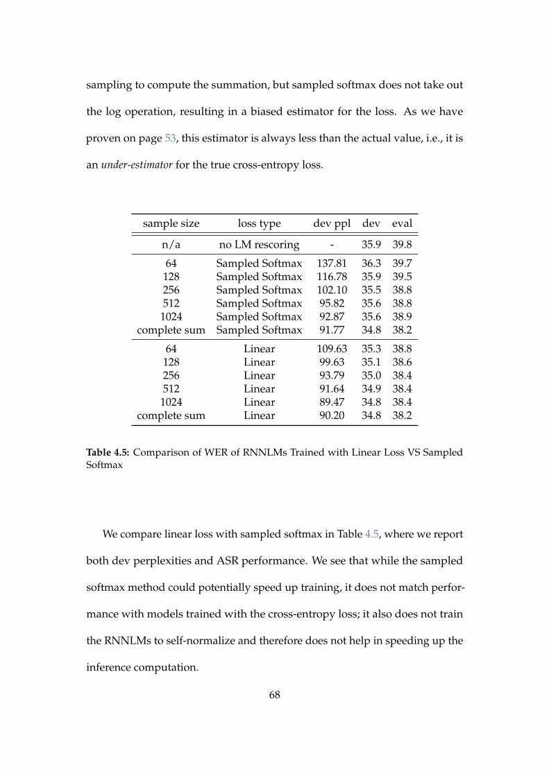
sampling to compute the summation, but sampled softmax does not take out

the log operation, resulting in a biased estimator for the loss. As we have

proven on page 53, this estimator is always less than the actual value, i.e., it is

an under-estimator for the true cross-entropy loss.

sample size loss type dev ppl dev eval

n/a no LM rescoring - 35.9 39.8

64 Sampled Softmax 137.81 36.3 39.7128 Sampled Softmax 116.78 35.9 39.5256 Sampled Softmax 102.10 35.5 38.8512 Sampled Softmax 95.82 35.6 38.8

1024 Sampled Softmax 92.87 35.6 38.9complete sum Sampled Softmax 91.77 34.8 38.2

64 Linear 109.63 35.3 38.8128 Linear 99.63 35.1 38.6256 Linear 93.79 35.0 38.4512 Linear 91.64 34.9 38.4

1024 Linear 89.47 34.8 38.4complete sum Linear 90.20 34.8 38.2

Table 4.5: Comparison of WER of RNNLMs Trained with Linear Loss VS SampledSoftmax

We compare linear loss with sampled softmax in Table 4.5, where we report

both dev perplexities and ASR performance. We see that while the sampled

softmax method could potentially speed up training, it does not match perfor-

mance with models trained with the cross-entropy loss; it also does not train

the RNNLMs to self-normalize and therefore does not help in speeding up the

inference computation.

68

4.4 Comparison with Sampled Variance Regulariza-

tion




64, S-VR train 75.89 0.9103 0.0260 0.1770dev 109.97 0.9163 0.0243 0.1700

128, S-VR train 60.77 0.9519 0.0315 0.1865dev 98.83 0.9559 0.0299 0.1808

256, S-VR train 58.43 1.0301 0.0245 0.1519dev 93.86 1.0325 0.0234 0.1483

512, S-VR train 54.71 1.0561 0.0226 0.1424dev 91.53 1.0593 0.0212 0.1373

1024, S-VR train 52.11 1.0935 0.0204 0.1306dev 89.83 1.0978 0.0197 0.1277

64, Linear train 70.80 0.9020 0.0332 0.2021dev 109.63 0.9064 0.0316 0.1960

128, Linear train 65.73 0.9560 0.0313 0.1850dev 100.55 0.9573 0.0312 0.1844

256, Linear train 58.22 1.0397 0.0318 0.1717dev 93.79 1.0419 0.0311 0.1694

512, Linear train 54.48 1.0778 0.0311 0.1638dev 91.64 1.0802 0.0296 0.1592

1024, Linear train 51.39 1.1178 0.0312 0.1581dev 89.47 1.1225 0.0310 0.1568

Table 4.6: Mean and Variance of Unnormalized Outputs in AMI with Sampling-basedTraining, Sampled VR VS Linear, Sampling with Replacement

In Section 3.3, we proposed to use importance-sampling on VR loss. We

report the experiments in Tables 4.6 and 4.7. We use hyper-parameter λ = 2.0

in all the sampled VR experiments.

69

From Table 4.6, we see that in most cases, the linear loss achieves compa-

rable but slightly worse perplexities than sampled VR, except the case with

1024 samples where the linear system slightly outperforms the corresponding

sampled VR system. Sample VR systems also seem to constrain the average

normalization terms closer to 1.0 and have smaller variance, but this depends

on the λ hyper-parameter we choose.

sample size loss type dev eval

n/a no LM rescoring 35.9 39.8

n/a cross-entropy 34.8 38.2

64 S-VR 35.4 38.9128 S-VR 35.1 38.8256 S-VR 35.1 38.7512 S-VR 35.0 38.5

1024 S-VR 34.8 38.4

64 Linear 35.3 38.8128 Linear 35.1 38.6256 Linear 35.0 38.4512 Linear 34.9 38.4

1024 Linear 34.8 38.4complete sum Linear 34.8 38.2

Table 4.7: Comparison of WER of RNNLMs Trained with Linear Loss VS Sampled VR

From Table 4.7, we see that again, the linear loss and the sampled VR loss

give very similar performances when used in the ASR task on the AMI-SDM

datasets.

70

4.5 Chapter Summary

In this chapter, we compared the linear loss proposed in Chapter 2 against

several commonly used loss functions in language modeling, both in terms of

perplexity on development data and word error rates in speech recognition

tasks. We have shown the superiority of the linear loss in both measures. We

also show that using sampling during training allows us to not compute the

whole summation term in the loss function, which can save much computation.

The sampling used in those experiments uses unigram distribution over the

vocabulary, and we allow the same word to be sampled multiple times during

each training step. In the next chapter, we perform a more comprehensive

study on sampling for language model training. We investigate the impact

of sampling specifications and propose more sophisticated sampling schemes

that improve the models’ performance.

71


72

Chapter 5

Impact of Sampling Algorithm on

Language Model Training

In Chapter 3, we described a training procedure for RNNLMs that uses importance-

sampling to speed up its computation. While sampling-based training could

save much neural-network computation, the sampling procedure adds com-

putational overheads, especially if it is not implemented efficiently. So far, in

all the reported experiments in previous chapters, we use a simple “sampling

with replacement” as the implementation. This is in order to get an initial idea

of the application of sampling in model training. In this chapter, we conduct

a study into the details of sampling algorithms and their impact on language

modeling, in performance and training speed.

73

5.1 Sampling with Replacement

In previous chapters, we have so far only considered the case of “sampling with

replacement”. This is perhaps the easiest sampling procedure to implement,

for it can be implemented as sampling one word from a unigram distribution k

times, where k is the desired number of samples. Algorithm 1 shows the basic

steps.

Algorithm 1: Algorithm for Sampling with ReplacementInput: k, p[1,...,n]Result: A Set S of size k

1 S = {}2 while |S| < k do3 s = sample a word according to p4 S = S ∪ {s}5 end6 return S

On line 3 of Algorithm 1, instead of naively performing a linear search

through the vocabulary, a more efficient binary-search version could be im-

plemented. With binary-search, this step requires a run-time complexity of

O(log(V)) instead of O(V)1, with V being the size of the vocabulary. Since line

3 will be performed precisely k times, this algorithm runs with a O(k log V)

complexity when line 3 uses a binary search algorithm. Moreover, if we could

afford more complex pre-processing of the sampling distribution, then a highly

efficient alias method [70] could be adopted in this sampling scheme, which

1The binary-search method also requires a one-time pre-processing of complexity O(V) tocompute a vector of accumulative sums of p.

74

runs in O(1) to generate one sample on line 3, and the run-time for generating

k samples would be O(k).

However, a problem with sampling with replacement is that it performs

duplicated computations if the same word appears more than once in the

sample. This almost always happens in real applications of this method. Take

English, for example – the most frequent word in English is “the” in most

domains; according to Google’s N-gram Viewer2, the unigram probability for

“the” has always been greater than 4.5% in the past 200 years. Hence, if we

train an English language model with a sample size greater than 44, we would

expect to see the word “the” in the sample at least twice. In our previously

reported experiments, we have shown that a sample size around 512 is needed

to achieve the best language modeling performance, and this would mean we

would expect to see the word “the” appear more than 23 times in the sample!

Furthermore, with the number of samples getting large, we would expect to see

duplications of many other less frequent words. Even in the case of sampling as

many words as the vocabulary-size, if we adopt the sampling with replacement

scheme, we will likely not see all words represented in the sample, but instead,

we will see frequent words appear multiple times in the sample and very few

infrequent words. This would result in wasted computation, not to mention

possible unnecessary estimation issues.

2https://books.google.com/ngrams

75

https://books.google.com/ngrams

5.2 Sampling without Replacement

We propose to use sampling without replacement as the sampling method.

By definition, this would solve the duplication issue and ensure that a word

appears at most once in any sample. However, by making this change, we now

have to be careful and redefine terms like the “sampling distribution”. Let us

take a look at one example to show how this could be an issue.

Again, we use the case of the word “the” mentioned above as an example –

let us assume that it has a unigram probability of 0.05, and we specify a sample

size of 512 words. We have seen that in the case of sampling with replacement,

it is expected that “the” would appear multiple times in the sample, since

0.05× 512 > 1. However, in the case of sampling without replacement, we

need to define the algorithm’s behavior to handles words like “the”. For

example, should we ensure that “the” will be sampled, i.e., with a sampling

probability of 1.0? Or should we assign a very high but still less-than-one

probability for it to be sampled? If we need to lower the probability for the,

how do we adjust the probabilities of other words? Those are non-trivial

questions but are essential in the design of the algorithm.

Sampling without replacement is a commonly used method for sampling in

statistics. This problem is formulated in two different ways, with very different

mathematical properties of the samples (except when the sampling distribution

is uniform, in which case the two formulations are equivalent). While we

76

will describe the details in later sections, we state here, with loosely defined

terms, that those two formulations differ because, due to the nature of sampling

without replacement, if we “sample from” a distribution, the “distribution of

the resulting samples” usually does not match the one from which we sample.

Given this distinction, some of the prior work, for example, [71], [72] focus

on sampling from a pre-defined distribution, while other works, such as [73],

[74] and [75], focuses on making sure the output samples match a pre-defined

distribution. Those works give an excellent analysis of the sampling methods’

statistical properties, but in general, are not focused on applying the methods

in a specific task, for example, in language modeling.

Following our previous results in Equation (3.19), we take the second ap-

proach of the interpretation for the problem, since in Equation (3.19), pi rep-

resents the probability that a word is included in the sample, which we refer

to as its inclusion probability. Say the vocabulary is V and we want to sample k

words. It is easy to see that, the inclusion probabilities for all the words in V

should sum up to k, i.e.

∑w∈V

P(w ∈ Sample) = k (5.1)

So the sampling procedure runs as follows:

1. we work out the “inclusion probabilities” of all words based on their

unigram probabilities and the number of samples we want;

77

2. we sample a set of words based on their inclusion probabilities.

For ease of presentation, in the following sections of this chapter, we first

visit the second step and then go back to the first.

5.3 Sampling without Replacement: Algorithm

In this section, we study one problem: given a positive integer k, a vocabulary

V = {1, ..., n}, and a list of inclusion probabilities for each word {p1, p2, ..., pn},

such thatn

∑i=1

pi = k

how should one sample a set S ⊂ V of distinct words, such that

|S| = k

and

∀i ∈ {1, 2, ..., n}, P(i ∈ S) = pi .

5.3.1 An Obvious (and Wrong) Approach

Most researchers, including the author of this dissertation, came up with a

very straight-forward algorithm for this problem, which unfortunately was

not correct. Since it is a common misconception, we demonstrate why it is not

correct in this section. The algorithm takes a simple “iteratively sample and

78

re-normalize” method, as shown in Algorithm 2.

Algorithm 2: An Incorrect Sampling-without-replacement AlgorithmInput: k, p[1,...,n]Result: A Set S of size k

1 S = {}2 while |S| < k do3 Z = ∑i/∈S p[i]4 re-normalize p by Z5 s = sample a word from p6 S = S ∪ {s}7 p[s] = 08 end9 return S

This algorithm runs reasonably efficient and would generate a set of distinct

k samples for every run; however, if we carry out the algorithm, then the actual

inclusion probabilities of words would not be equal to the specified ones.

We demonstrate that with a simple example of selecting two samples from a

vocabulary of size 3.

Say we have

(p1, p2, p3) = (0.5, 0.5, 1) (5.2)

Then the desired probabilities for selected subsets of words should be

p({1, 2}) = 0

p({1, 3}) = 0.5

p({2, 3}) = 0.5

(5.3)

However, we can easily see that if we follow Algorithm 2, then in the first

79

iteration of the while loop, there is a probability of 0.5 that word 1 is sampled;

then in the 2nd iteration, there is a probability of 13 that word 2 get sampled.

This would give

p({1, 2}) > 16> 0,

which does not equal the probabilities we specified. Note that this is a simple

example to demonstrate the algorithm is incorrect by devising a case where

certain combinations of words are not possible. However, this algorithm is

wrong even in the most general cases, even when all combinations allowed in

the sample.

5.3.2 Reservoir Sampling Algorithm

[75] proposed an algorithm that correctly solves the problem, which is com-

monly referred to as the reservoir sampling algorithm. It is a rather complex

algorithm, and we only show its main structure in Algorithm 3 (upon which

we make improvements in later sections) and omit some of the details.

Algorithm 3 works by first picking the first k words in the set and then

iterates over all the remaining words. When seeing a new word, it first makes

a random decision whether to add this new word in the set. If not, it goes on

to decide for the next word; otherwise, it randomly picks an existing word

to be replaced by the new. We omit the details of computing the vector R,

representing the replacement probability for each existing word. The detail of

computing the vector R is presented in [75]. The key is setting them so that at

80

Algorithm 3: Reservoir Sampling Algorithm (incomplete)Input: k, p[1,...,n]Result: A List S of size k

1 S = [1, 2, ..., k] for i← k + 1 to n do2 decide with probability p[i] whether to include i in S3 if decided to add i then4 compute R[1, ..., k] (refer to paper for details)5 randomly pick j ∈ {1, ..., k} according to R6 S[j] = i7 end8 end9 return S

the end of each iteration of the for loop, the inclusion probability of any word

w up to the current index i is proportional to its desired inclusion probability in

p[w] so that after the last iteration, the inclusion probability of all words would

correspond to the values specified in p.

An analysis of the algorithm reveals that its worst-case time complexity is

O(nk), n for iterating over all words, and k for computing vector R of length

k. We notice that the computation of R is only needed if we decide to add the

new word to the set, and the probability of that depends on the new word’s

inclusion probability. We can take advantage of that and make the algorithm

faster (in terms of average time complexity) by arranging the word orders such

that the p[i] is descending for i. Of course, sorting would add complexity of

O(n log n) to the algorithm, but in the case where we pre-process once and

then sample multiple times, this one-time cost will be amortized, leading to

significant speed-ups.

81

5.3.3 2-stage Reservoir Sampling Algorithm

One benefit of the reservoir sampling algorithm is that it introduces minimum

dependencies among different words. Note that, since we are sampling a fix-

sized set, certain dependencies between words are inevitable, and one example

would be the previous example shown in Equation (5.2), wherein the solution

Equation (5.3), we see that 1 and 2 can never be sampled simultaneously.

This type of dependency is inevitable because of the nature of the “n choose

k” problems. However, it can be shown that this algorithm adds no other

dependencies in the output than the problem imposes; again, interested readers

should refer to [75] for details.

A significant problem of the algorithm is the n term in its complexity. This is

because, in practice, n could be in the hundreds of thousands or even millions.

We now propose a modification that does not need to iterate over all words.

We achieve this by adding more dependencies in the output, which we call a

2-stage sampling algorithm.

Here is how the 2-stage sampling algorithm works: we first divide the

vocabulary {1, 2, ..., n} into m disjoint subsets s1, s2, ..., sm, where

p(si)def= ∑

j∈si

p(j) ≤ 1.0, ∀i ∈ {1, 2, ..., m}

The grouping operation could be simply implemented with a greedy al-

gorithm, as shown in Algorithm 4. To simplify the procedure and improve

82

efficiency, we only group words with consecutive indices, which is usually

arbitrarily chosen, and does not affect the correctness of the algorithm.

Algorithm 4: Placing Words into Groups for 2-stage SamplingInput: p[1,...,n]Result: g[1,2,...,m], each element is a group represented as a set

1 idx = 02 g_idx = 03 g_probs = [0.0]4 g = []5 while idx < n do6 if g_probs[g_idx] + p[idx] ≤ 1.0 then7 g[g_idx].insert(idx)8 g_probs[g_idx] = g_probs[g_idx] + p[idx]9 else

10 g_idx++;11 g[g_idx].insert(idx) g_probs[g_idx] = p[idx]12 end

13 end14 return g

After the grouping, we do the sampling. In the first stage, we sample k

groups according to group inclusion probabilities p(s); in the second stage, we

pick precisely one element from each group, with probabilities proportional to

word inclusion probabilities in this group.

It is not hard to see that this algorithm is “correct” in that, the probability

for any word w being sampled is p(w): first we need to sample the group s

where w ∈ s, with probability p(s) = ∑i∈s p(i); then we need to pick w from

the group, with probability p(w)p(s) , and the algorithm is correct because,

p(s) · p(w)

p(s)= p(w).

83

However, we also see that this modification adds unnecessary dependencies

between words – for example, two words in the same group would never be

simultaneously sampled.

Now we analyze the complexity when the grouping {s1, s2, ..., sm} is already

given. In the first stage, we sample k groups from m groups, and so it has a

complexity of O(km). It is hard to perform a rigorous analysis in the second

stage because we do not know the grouping information. Nevertheless, sam-

pling one from multiple words could easily be implemented with a binary

search algorithm3, which is logarithmic w.r.t. group sizes. Suppose the group-

ing is close to evenly, then each group would have nm elements, and then the

complexity for the second stage is

O(k lognm)

This will give a total complexity of

O(km) + O(k lognm) = O(k(m +

nm)) = O(k max(m,

nm))

This analysis under simple assumptions also shows that a good choice of

the number of groups to use would be around√

n. We can generalize this

method to 3-stage (or even 4 or above), and the optimum number of groups

3Although the alias method gives better performance than binary search, as in later chapters,we will not always sample from the same distribution; therefore the alias method is not suitedfor our experiments.

84

would then be around n13 , but the efficiency improvement would be marginal

compared to the computation overhead.

5.3.4 Systematic Sampling Algorithm

Another sampling method with added dependencies is the systematic sampling

algorithm method proposed in [76]. This algorithm is best explained with a

visual aid shown in Figure 5.1. Figure 5.1 shows a 2-D space with X and Y

axes. For each word i with inclusion probability pi, there is a rectangle of size

[1× pi], where 1 is the width on the x-axis, and pi is the height on the y-axis. In

the figure, we have assigned different words with different colors. Because we

have

∑i

pi = k

We can now put the rectangles for all words at the corner of the 1st quadrant,

and by possibly cutting rectangles for certain words horizontally, arrange all of

them fit in the shape of a larger rectangle [k× 1]. In the example in Figure 5.1,

we cut the rectangles with the colors orange, dark blue, and purple, and all of

those rectangles fit in the space of [6× 1].

Now we uniformly choose a random number r between 0 and 1 and draw a

line y = r on the rearranged rectangles, as shown with the dotted line in Figure

5.1. This line would touch exactly k rectangles 4. The words corresponding to

4In order for this to be well-defined, we shall also define what “touch” means. It mightvary with implementation, but an easy way would be to consider each rectangle as taking aleft-close and right-open space, except the top-rightest one, which is close for both left and

85

Figure 5.1: Visual Aid to Help Understand the Systematic Sampling Algorithm.

those rectangles are then the sampled words. Since we draw a random number

from a uniform distribution between 0 and 1, the probability of sampling a

word is proportional to its “height” in the diagram, and thus we guarantee

that this method also satisfies the inclusion probability conditions. Also, it

introduces strong dependencies in the distribution of the sampled words,

and the relative position of rectangles determines this dependency after the

rearrangement. For example, if the arrangement is like that in Figure 5.1, then

we know that if the word represented by the light-blue color is sampled, then

we know for sure that the words represented by red will be sampled, and the

word represented by yellow will not be sampled.

Now the complexity: This algorithm requires us to search for precisely

one rectangle at k different height levels, and each of those searches could be

right. The exact choice does not matter theoretically since the probability of cutting “exactlyon the boundary” is always zero; however, in practice where numbers are represented inapproximations, e.g., the floating-point number representation, this might make some edgecases more complicated than in theory.

86

implemented as a binary search. On average, each height level would have

nk + 1 rectangles5. So the complexity would be

O(k log(nk+ 1))

Note this method is a continuous (as opposed to discrete) version of the 2-

stage method – because we can divide the probability mass w.r.t. one word into

different parts, the algorithm can start with exactly k “groups”. The difference

is, in order to avoid picking the same word in 2 different groups (since a word

can now be in two groups), the algorithm does not independently sample from

each group but jointly does so, avoiding the possibility of sampling one word

twice.

5.3.5 2-stage systematic sampling

We can also apply the 2-stage idea for the systematic sampling algorithm, where

we use systematic sampling in the first stage to sample groups. However, a

simple analysis of this method would reveal that this does not change the

Big-O complexity of the algorithm – since in both stages, the search could be

efficiently implemented as a binary search, if we adopt a 2-stage sampling

method.

However, there is still merit in performing 2-stage sampling with systematic

5we have +1 because, with high probability, each original rectangle would be cut in 2,though each level would on average have one more rectangle

87

sampling. The reason is, so far, we only sample from a unigram distribution,

which allows the opportunity to pre-process the distribution – computing a

vector storing the cumulative sums of the unigram probabilities to perform

an efficient binary search. However, if we want to repeatedly sample from a

(slightly) different distribution every time, then we could not afford to perform

the pre-processing every time before sampling. However, using the 2-stage

sampling method could alleviate this issue. More details are shown in Chapter

6.

5.4 Computing Inclusion Probabilities

In the previous sections, we assumed that the inclusion probabilities are already

given and studied algorithms to sample from such distributions. In this section,

we study how to generate inclusion probabilities for a vocabulary, given their

unigram probabilities and the sample-size we want. Note that the algorithm we

propose could be used to compute inclusion probabilities for not just unigrams

but higher-order models as well, and we pick unigrams to make it easy to

describe the method.

Say we have a vocabulary V = {1, 2, ..., n}, and a unigram distribution

u(.) on V. Our task is to compute a vector of inclusion probabilities pi, where

pi represents the probability of selecting word i in the sample. In the case

of sampling k words from a vocabulary of size n, the pi’s need to somehow

88

“reflect” the unigram probabilities, while satisfying the following constraints,

n

∑i=1

pi = k (5.4)

and

0 ≤ pi ≤ 1, ∀i = 1, ..., n. (5.5)

This problem is an open-ended one, to which there is not one single “cor-

rect” solution because the inclusion probabilities could “reflect” the unigram

distribution in different ways. One primary reason that we want the sample to

reflect the real distribution is in Equation 3.19, where we show that we could

minimize the variance in the sampled estimator if the sampling distribution

is proportional to the actual distribution. In our case, we use the unigram

distribution as a proxy for the actual distribution, and thus an ideal setup for

the inclusion probabilities is

pi = kui, ∀i.

This guarantees that for every word in the vocabulary, the probability of

it getting sampled is proportional to its unigram probability; however, in real

languages, the unigram probabilities for different words vary by a lot, and

setting the inclusion probability to be proportional to unigrams, the most

frequent words in the language would usually have an inclusion probability of

greater than one, which violates Equation 5.5, and the pi’s do not represent valid

probabilities any more. The statistics on the word “the” in English described in

89

Section 5.2 is an excellent example of this issue.

The solution we propose is to distribute the excess probability mass of

frequent words to less frequent words proportionally to their unigram prob-

abilities. In this procedure, we first compute a P = [p1, p2, ..., pn], where

∀i ∈ V, pi = ui · k, so some of the numbers might be larger than one. We

perform the normalization in Algorithm 5.

Algorithm 5: Inclusion Probability Normalization AlgorithmInput: k, p[1,...,n]Result: normalized p[1,...,n]

1 m = argmaxi p[i]2 while p[m] > 1.0 do3 d = p[m]− 1.04 p[m] = 1.05 s = k− p[m]6 for i← 1 to n do7 if i = m then8 p[i] = p[i] + d× p[i]/s9 end

10 end11 m = argmaxi p[i]12 end13 return p

Algorithm 5 works by picking words whose inclusion probabilities are

greater than one and proportionally distribute the extra probability mass to

all other words, proportional to their unigram probabilities. This procedure

needs to be carried out iteratively until there are no words with larger-than-one

inclusion probabilities. We need such an iterative algorithm because even if

a word initially has an inclusion probability smaller than 1.0, it might end up

larger than one after acquiring some of the probability mass from other words.

90

Fortunately, this algorithm is guaranteed to terminate – a simple way to see

that is, this algorithm guarantees that the difference between the largest and

the smallest p[i]’s is decreasing after each iteration, and the worst-case scenario

would be the “n choose n” case, where the final inclusion probability vector

contains all 1’s no matter what the initial values are6.

5.5 Evaluation of Different Sampling Methods

In this section, we compare the different approached mentioned in this chapter

in terms of efficiency.

We compare the speed of running different sampling algorithms by sam-

pling from a unigram distribution in Table 5.1. In those experiments, we

randomly generate unigram probability distributions for the specified vocabu-

lary and then normalize the generated distribution according to Algorithm 5.

For 2-stage sampling algorithms, additional processing is performed to break

the vocabulary into groups. This is done by following the greedy algorithm rep-

resented in Algorithm 4. For the “sorted” experiments, we sort the vocabulary

once according to their inclusion probabilities in a descending way. Since we

only sample from the same unigram distribution, the pre-processing steps only

need to be done once in the beginning. We report the run-time, in seconds, of

running the same sampling procedure of “sampling k words from a vocabulary

6We point out here that, again, this is the result of purely theoretical analysis. In the case offloating-point numbers, depending on the details of implementation, it is possible that this “nchoose n” would never terminate, and special attention is needed in the implementation of thealgorithm to avoid such issues.

91

of size n” exactly t times.

n, k, t reservoir systematic

std sorted 2-stage std 2-stage

100000, 50, 100 0.256 0.288 0.032 0.016 0.008100000, 100, 100 0.376 0.388 0.04 0.016 0.008100000, 250, 100 1.032 0.968 0.044 0.012 0.016100000, 500, 100 3.112 2.952 0.056 0.02 0.012

100000, 1000, 100 9.94 9.228 0.088 0.028 0.024100000, 2000, 100 33.592 28.364 0.208 0.036 0.036100000, 4000, 100 113.864 87.208 0.704 0.044 0.06

100000, 10000, 100 514.148 354.064 7.648 0.084 0.116100000, 20000, 100 1473.72 867.288 86.472 0.128 0.176100000, 40000, 100 3536.45 1488.59 761.188 0.196 0.276

10000, 50, 1000 0.488 0.468 0.056 0.008 0.01210000, 100, 1000 1.132 1.056 0.08 0.012 0.01610000, 250, 1000 5.076 4.316 0.128 0.02 0.02810000, 500, 1000 16.08 12.932 0.2 0.036 0.06

10000, 1000, 1000 48.012 35.58 0.36 0.052 0.09610000, 2000, 1000 138.936 87.74 1.132 0.104 0.1410000, 4000, 1000 323.832 146.00 6.276 0.172 0.26

Table 5.1: Time (of t runs of n choose k in seconds) of Sampling from Unigrams

For reservoir sampling, as shown in columns 2 to 4 in Table 5.1, we have

the following observations.

1. sorting the vocabulary helps reduce the run-time of the algorithm for

most of the experiments. However, in a few cases where the number of

samples is small, it takes more time than the unsorted version, and this

is due to the added cost of sorting the vocabulary – when we only want

a small number of samples, this added cost is too high for the efficiency

improvement to compensate.

92

2. while sorting brings a small improvement to the speed of the algorithm,

the 2-stage method brings significant speed-up to the original algorithm;

depending on the actual configuration, this speed-up ranges from one

order of magnitude (e.g., the first row) to two orders of magnitudes (e.g.,

the second-to-last row).

Now we analyze columns 5 and 6 for the systematic sampling algorithm.

We see the following,

1. Compared to the reservoir sampling method, the systematic algorithm

is much faster. In the extreme case of a large number of samples, it is

3536.45/0.276 = 12813 times faster than the reservoir algorithm.

2. the 2-stage version of the algorithm slows down the computation – this

is no surprise, as our analysis showed that the 2-stage algorithm has the

same complexity as the original 1-stage algorithm in terms of Big-O order,

however, because the added overhead of the 2-stage algorithm, it would

result in a larger constant in the complexity that is hidden in the Big-O

notations.

5.6 Language Modeling Experiments

In this section, we perform a simple set of experiments investigating the differ-

ence of different sampling methods in the task of language model training. We

use the aforementioned PyTorch RNNLM implementation as a starting point,

93




64, NR train 65.03 0.9533 0.0326 0.1893dev 100.69 0.9525 0.0331 0.1911

128, NR train 59.25 1.0360 0.0256 0.1544dev 95.32 1.0424 0.0250 0.1518

256, NR train 54.52 1.0997 0.0346 0.1692dev 92.01 1.1040 0.0336 0.1659

512, NR train 49.10 1.1361 0.0436 0.1838dev 89.12 1.1428 0.0429 0.1812

1024, NR train 46.25 1.1823 0.0504 0.1899dev 89.26 1.1892 0.0518 0.1914

64, R train 70.80 0.9020 0.0332 0.2021dev 109.63 0.9064 0.0316 0.1960

128, R train 65.73 0.9560 0.0313 0.1850dev 100.55 0.9573 0.0312 0.1844

256, R train 58.22 1.0397 0.0318 0.1717dev 93.79 1.0419 0.0311 0.1694

512, R train 54.48 1.0778 0.0311 0.1638dev 91.64 1.0802 0.0296 0.1592

1024, R train 51.39 1.1178 0.0312 0.1581dev 89.47 1.1225 0.0310 0.1568

Table 5.2: Comparison between Different Sampling Methods

and implement the different schemes described in previous sections that uses a

pre-computed unigram distribution as the sampling distribution.

5.6.1 The Impact of Replacement

We report the training stats on the AMI corpus in Table 5.2 with two types of

sampling procedures, namely sampling with replacement (R) and sampling

94

without replacement (NR). As described before, in the R scheme, we could

sample the same word multiple times for the same batch, which makes it

easier to implement the sampling algorithm, but there could be a duplicate of

computation; when we sample without replacement (NR), there is no duplicate

of the same word in the sampled set.

From Table 5.2, we see that, in general, the sampling-without-replacement

methods yield better perplexities than sampling-with-replacement for all sample-

sizes, and with more significant differences for smaller sample-sizes. This is

expected since, in the sampling-without-replacement approach, the generated

samples have no duplicates and cover more vocabulary words. We also see

that sampling-without-replacement methods result in slightly higher variances

for the normalization term. This is explained by the fact that, for the sampling-

without-replacement approach, the inclusion probabilities of words are not

always proportional to their unigram probabilities, thus resulting in higher

variances, following our analysis done in Section 3.2.3.

5.7 Chapter Summary

In this chapter, we focus on the sampling algorithm used in importance-

sampling based language model training. We present algorithms for sampling

with and without replacement and propose improvements on the sampling-

without-replacement algorithm, making it more efficient. We also present an

algorithm for normalizing the inclusion probability vector used in the sampling-

95

without-replacement algorithm.

We present our experimental results comparing the efficiency of differ-

ent sampling algorithms and comparing their performance in language mod-

eling tasks. We show that our proposed 2-stage sampling method gives

significant speed-up over the unmodified baseline algorithm and that us-

ing a sampling-without-replacement scheme outperforms the sampling-with-

replacement scheme in language modeling tasks.

96

Chapter 6

Batch Training and Sampling from

Longer Histories

In previous chapters, we have proposed using importance-sampling to help

speed up RNNLM training with the linear loss and reported experimental

results, where we compared the linear loss with some other loss functions and

investigated the impact of different sampling algorithms.

Recall in Equation (3.19) on page 55, where we have shown that to minimize

the variance of the loss estimator computed from sampling, the sampling

distribution need be proportional to the “true” distribution of data. In all the

experiments we have reported, we use simple unigram distribution as a proxy

for the true distribution. While not necessarily the optimal distribution, this

allows smooth interaction between the sampling-based training and batch-

based training – by sampling from a unigram distribution and not considering

97

any history information, different examples in a batch may share the same

samples, which helps improve the computational efficiency of model training.

At this point, readers might not be convinced of the importance of including

longer histories, especially since we have demonstrated with our previously

reported experiments that reasonably good performance could be achieved

with sampling from unigrams. While we will conduct detailed experiments,

comparing results with different sampling distributions, here is an intuitive

explanation for why the history might matter.

Let us take English as an example and consider the word “San”. Say a sen-

tence contains the phrase “San Francisco”, and the model now is computing the

loss for the word “Francisco”. We know that words like “Jose”, “Bernardino”

and “Diego” all have relatively low unigram probabilities but frequently occur

after “San”. To accurately estimate the normalization term for history “San”, it

would be essential to include those words in the sample. However, sampling

from a unigram distribution would make this very unlikely, making the esti-

mated normalization term deviate from the actual value; On the other hand, if

we sample from a bigram in this case, then it is much more likely that all those

words get sampled, leading to a more accurate estimator for the loss function.

This chapter discusses how to incorporate longer history information in

the sampling-based training scheme, for example, sampling from a bigram

distribution. In the case of training on one example at a time, it is trivial to

change the training scheme to support sampling from bigrams; however, it is

98

not the case for batch-based training. This is because different examples in the

same batch usually have different histories, so we can not make all examples in

the batch share the same samples; it is possible to generate different samples for

different examples in the same batch, adding unwanted computation overheads

and is therefore not ideal.

To balance the improved computational efficiency of batch training and the

more accurate estimation with history information, we propose generating the

sampling distribution from the average of all the n-gram distributions in the

batch.

6.1 Average n-gram Distribution in a Batch

Let us view all examples in a batch B as a set of (history, word) pairs, denoted

as (h, w).

B = {(h, w)}

By pre-training an n-gram model on the training data, each h would correspond

to a probability distribution over the vocabulary by truncating history and

retaining only the last n− 1 words. We denote the distribution for history h as

99

Pn(.|h). Then, we set the sampling distribution 1 s(.) for this batch as,

sB(w) =1|B| ∑

(h,w)∈BPn(w|h) (6.1)

6.2 Sampling with Longer Histories

Previously in Chapter 5, we introduced efficient algorithms to sample from a

unigram distribution, which involves a one-time pre-processing of the distribu-

tion, which the efficient sampling algorithm needs. A side effect of using longer

histories as the sampling distribution is that now we sample from different

distributions for different batches, so it is no longer possible only to pre-process

once and reuse the output of pre-processing for all later computations. Here we

propose a method that achieves the middle ground – a sampling algorithm that

involves a one-time pre-processing step and supports sampling from different

run-time distributions while still being efficient.

Note that the method we propose is not a general-purpose sampling scheme

that supports any run-time distribution but operates under the assumption that

while the run-time sampling distributions might differ, their differences are

relatively small. To achieves this, we first perform a highly selective pruning

procedure over the higher-order n-grams. The pruning works by removing

certain higher-order n-grams if they do not meet the specified criteria, and

1Readers are reminded here that sampling distribution is not the distribution we samplewords from, but rather a starting point to generate the inclusion probability distribution, whichthe sampling algorithms use. More details are in Section 5.4.

100

we use their back-off lower-order n-gram probabilities instead. For example,

if bigram p(A|B) does not meet our criteria and is pruned away, then the

sampling probability of A with history B will be its unigram probability P(A); if

trigram P(A|BC) is pruned away but P(A|C) is not pruned, then the sampling

probability of A with history BC will be its bigram probability P(A|C).

The pruning criteria is the following,

1. we prune away p(w|w1, ..., wn−1) if the ratio

p(w|w1, ..., wn−1)

p(w)

is smaller than a threshold, and we set this threshold to be 100;

2. for n > 2, we prune away p(w|w1, ..., wn−1) if its ratio to its immediate

backoff n-gram, i.e.

p(w|w1, ..., wn−1)

p(w|w2, ..., wn−1)

is smaller than a threshold, which we set as 2.

The intuition behind the pruning idea is, given a history, if the higher-order

n-gram probability of a word is significantly larger than its back-off n-gram

or unigram, then we need to raise the sampling probability of this word by

keeping its higher-order n-gram. Otherwise, we would not likely sample this

word and significantly underestimate the normalization term in our estimation.

After the pruning is performed, for any history h, most of the words w

101

in the vocabulary would rely on backing off to their unigram probabilities in

generating their sampling probabilities. By backing off, we do not mean directly

using their unigram probabilities, but instead, take the unigram probabilities

and multiply by a factor to make sure the sum of probabilities for all words

add up to one. This is part of the standard methods with a back-off n-gram

model, and readers could refer to [77] for more details.

Note that in previous chapters, we pre-process the unigram probability

vector to compute a vector of accumulative sums, on which we perform a

binary search in run-time to save computation. Now, because we might have

a different distribution at run-time, such an accumulative sum vector is dif-

ferent each time. We use the 2-stage sampling method described in Chapter 5

for sampling and propose the following method to avoid adding substantial

computational overheads for higher-order n-grams. Here is an outline of the

2-stage sampling method,

• Pre-processing

1. Generating grouping structures

2. Compute accumulative sum vector for groups

3. Compute accumulative sum vector for within each group

• Run-time

1. pick groups according to group accumulative sum vector

102

2. pick a word from each selected group using its accumulative sum

vector

For sampling with n-grams, its outline is slightly different,

• Pre-processing

1. Generating grouping structures

2. Compute accumulative sum vector for within each group

• Run-time

1. Re-grouping

2. pick groups according to the output from step 1

3. pick a word from each selected group using its accumulative sum

vector

The pre-processing step is almost identical to the unigram case, and the

only difference is that we do not compute the accumulative sum vector for

groups since it is not needed.

At run time, the first step is to perform a procedure that we call re-grouping.

Say the current history is h, and we first identifies all words w following this

history whose probabilities do not back off to unigrams. We find the groups

they belong to for all those words and change the structures for those groups

by further dividing them into subgroups. The result of the re-grouping is that

each resulted group would contain only a single word that does not back off

103

Figure 6.1: Changing group assignments for words when changing the sampling distri-bution from unigrams to higher-order n-grams. The group containing words w1, ..., w7is divided into 4 groups since w1 and w4 have higher-order n-gram probabilities.

to unigram, or a consecutive block of words, all of which back off to unigram.

Note we do not change the relative ordering of the words in this group.

An example of this is shown in Figure 6.1. In this example, we have a group

with words w1, ..., w7, and the words marked in red, namely w1 and w4, do not

back off to unigram. We then further divide the group into four subgroups: w1

and w4 both become single-word groups. Two more groups are formed that

consist of back-off words, one for {w2, w3}, and the other for {w5, w6, w7}.

The second step is to pick k groups from all groups. For this step, we need

to generate the accumulative sum vector for the groups from scratch each time.

This was carried out in pre-processing steps for unigram 2-stage sampling

since the group probabilities do not change. This step is the primary overhead

that this algorithm introduces. Also, we note that the number of groups now is

larger than the unigram sampling case because step 1 of the algorithm would

increase the number of groups. A careful analysis shows that the increase for

104

the number of groups is bounded by 2d, where d is the number of words that

do not back off to unigram. This is because, in the re-grouping step, a word

that does not back off to unigram adds at most two additional groups in the

algorithm. Therefore, as long as we prune the n-gram language well, this step

does not add substantial overhead to our computation.

The last step is to pick precisely one word from each sampled group. Be-

cause in the grouping restructure step, we do not change the relative ordering

of the words, we could reuse the pre-computed accumulative sum vector for

computation.

6.3 Experiments

In this section, we report experiments that compare sampling from a unigram

distribution versus from distribution with histories, including bigram and

trigram histories. The experiments reported in this section are conducted with

Kaldi, and the RNNLM implementation uses Kaldi-RNNLM [78].

We first report experiments on the AMI dataset. The data preparation of

this dataset follows the provided script [79] in Kaldi. Note that this script has

its way of dividing the training and development data, and thus the reported

perplexities on the development set are not comparable with the previously

reported AMI numbers. The results are in Table 6.1.

We also report the rate of convergence comparing unigram, bigram, and

105

num-samples n-gram order perplexity mean

128 1 58.3 1.13128 2 53.6 1.09128 3 51.9 1.06256 1 51.4 1.09256 2 49.7 1.08256 3 49.1 1.07512 1 49.4 1.08512 2 48.4 1.08512 3 48.0 1.07

Table 6.1: Effect of Sampling From Longer History in Switchboard

trigram-based sampling, for the setup using 256 samples in Figure 6.2, where

we plot the cross-entropy loss on the development set.

Combining the information from Table 6.1 and Figure 6.2, we have the

following observation,

1. Including history information for sampling helps improve language mod-

eling performance as measured by dev perplexity.

2. Including history information also helps bring the mean of the normal-

ization term closer to one; this effect is more pronounced for models with

fewer samples.

3. History information also helps improve the convergence rate during

training.

4. For all the observation above, we have seen that using a bigram language

model is better than unigram, and trigram would be better than bigram.

106

Figure 6.2: Convergence Rate VS Sampling Distribution

6.4 Chapter Summary

This chapter identifies the potential problem of the sampling-based method

introduced in previous chapters, which uses a unigram probability distribution

for sampling. We propose to include history to improve the sampling-based

RNNLM training and sample from an n-gram distribution based on the context.

We propose an efficient method that computes the average n-gram distribu-

tion based on all histories in the batch and makes the examples in the same

batch share the same samples. This makes the computation tractable, and

experiments show that including history information in the sampling step

leads to better language models’ performance measured by perplexity on the

development set. It also pushes the average normalization terms closer to one.

107

This concludes the first part of this thesis, which is primarily on improving

the computational efficiency of RNNLMs, both for training and inference

computation. In part II, we introduce methods to improve the computational

efficiency of applying RNNLMs in lattice rescoring for speech recognition.

108

PART II:


EFFICIENCY OF RNNLM LATTICE

RESCORING

109

Part II Outline

Various techniques to make the RNNLM computation more efficient both in

training and inference were studied in Part I. We focus in Part II on applying

RNNLMs in speech recognition tasks. We study the commonly used lattice-

rescoring method for applying an RNNLM and propose improvements to

the algorithm, making it more computationally efficient. This part includes

Chapters 7 and 8. We first give a gentle introduction to finite-state transducers

in Chapter 7, which lays the foundation of the lattice-rescoring algorithm on

which we focus. We then introduce the standard lattice-rescoring algorithm

using the FST framework and the commonly used n-gram approximation

method for applying an RNNLM in lattice rescoring, which serves as the

baseline method upon which we try to improve. We then introduce the pruning

algorithm for lattice-rescoring and report our experimental results.

110

Chapter 7

Lattice Rescoring in the FST

Framework

We begin with a brief introduction to Finite-state transducers (FST)1, with which

lattice rescoring methods are usually implemented. FSTs are commonly used in

most major hybrid speech recognition systems. They elegantly unify Hidden-

Markov Models, the use of context-dependent phones, pronunciation lexicon,

and an n-gram language model into one decoding graph, each of which may

be represented using an FST, and may be amalgamated into a single FST,

using the FST-composition operation, while preserving all the information of the

individual FSTs. Although the FST framework is not necessary for building an

ASR system, and it does not add any additional modeling power, it dramatically

1We follow the convention in the speech community that when we say FST, it usuallymeans weighted finite-state transducer or WFST, except when we make clear we are talking aboutunweighted FSTs.

111

reduces the amount of work by researchers by providing a level of abstraction

and makes the system easier to understand and implement.

This chapter is not a comprehensive description of FSTs and FST operations

but a gentle introduction to the necessary concepts to understand our proposed

algorithms in the next chapter. Interested readers are referred to [23, 80] for

details on FSTs. In this chapter, we first introduce a finite-state automaton, which

may be viewed as a special (and simple) version of an FST; then, we talk

about FSTs and the composition operation, which serves as the foundation of

the standard lattice-rescoring algorithm and the pruned improvement that we

propose in Chapter 8.

7.1 Finite-state Automaton

In plain natural language, a finite-state automaton represents a graph with a

finite number of nodes connected with directed arcs. Let us take a look at a

real-life example in Figure 7.1. Although simple, this diagram is a surprisingly

realistic depiction of all those years of working on a Ph.D. experienced by the

author.

We can see the following from the diagram.

• It has three states;

• It has four arcs connecting from a state to another;

• On each arc, there is an associated label.

112

Figure 7.1: Diagram depicting the author’s experience of working on a Ph.D. It consistsof three states and four directed arcs connecting one state to another. This diagramdoes not satisfy the condition for finite-state automata because it does not have a startstate and a final state.

However, Figure 7.1 does not yet satisfy the condition for an FSA. Two

additional requirements are needed in order to make a mathematically well-

defined FSA.

• It needs to have a start state;

• It needs to have one or more final state[s];

If we take Figure 7.1 and change it slightly to Figure 7.2 by adding a start

state and final state, along with necessary arcs that connect them to the original

diagram, then it is a valid FSA.

Mathematically, an FSA is a 5-tuple, (Q, Σ, I, F, δ), where

• Q is a finite set of states;

• Σ is a finite alphabet set;

• I ⊆ Q is the set of initial states;

• F ⊆ Q is the set of final states;

113

Figure 7.2: A finite-state automaton depicting the author’s experience of working onPhD. It consists of five states, and 6 directed arcs connecting one state to another. Thestart state is represented by the double circle and the final state is represented by thetriple circle.

• δ ⊆ Q× (Σ∪{ϵ})×Q is the set of arcs. (ϵ represents the “empty” symbol,

or lack of a symbol)

The details of the definition might vary. For example, some definitions

require that the cardinality of I or F must be exactly 1. Nevertheless, those

constraints do not hamper the modeling capacity of an FSA. 2

We could extend the definition of an FSA to weighted finite-state automaton

(WFSA), where associated with each arc in δ, there is a weight. The domain of

the weight is any semi-ring, and readers may refer to [81] for more details.

2By this, we mean that if an FSA A under one definition breaks some constraint of a differentdefinition of FSA, then we could easily reconstruct another FSA A′ that is mathematicallyequivalent.

114

7.2 Finite-state Transducer

Finite-state transducers (FST) are a generalization of FSAs, where instead of just

one symbol associated with an arc, now there is a separate “input symbol” and

“output symbol”. Note that an FSA could be seen as a special case of FST where

the input and output symbols are always identical. Similarly, we expand the

definition of (unweighted) FSTs to weighted finite-state transducers (WFST) by

making each arc associate with a weight.

There are two common ways to view a WFST. Firstly, a WFST represents a

function3

si → (so, w) (7.1)

In the second way, a WFST represents a function,

(si, so)→ w (7.2)

In both interpretations, si represents an input sequence, so an output se-

quence; and w a weight. In the first interpretation, it means that the FST takes

input si and transduces it to so, with weight w; in the second interpretation, it

means that the FST “accepts” the sequence pair (si, so) with weight w.

3Strictly speaking, a function needs to be right-unique [82], meaning there should be aunique output for a given input; this is not always the case for general FSTs since FSTs alsosupport one-to-many mapping; but within the scope of this thesis, the WFSTs we use arealways deterministic and thus always represent a function.

115

7.3 FST Composition

Composition is an operation on FSTs that combines two transductions. If FST

A transduces sequence x to sequence y, and FST B transduces y to z, then the

Composition of B and A, represented by B ◦ A, transduces x directly to z. FST

composition is an important operation that combines FSTs that operate on

different layers of representations. For example, in a typical speech recognition

system, there are four different FSTs, namely H, C, L, and G. The four FSTs

represent the HMM topology that transduces from phone-states to context-

dependent phones, context-dependency that transduces context-dependent

phones to monophones, a lexicon that transduces monophones to words, and

finally grammar, which is usually an FSA that we use to compute the weight

of word equences4), respectively. By composing all four FSTs, we generate a

decoding graph HCLG,

HCLG = H ◦ C ◦ L ◦ G, (7.3)

which transduces phone-state sequences directly to word-sequences and output

the associated weights. The information provided by such a decoding graph

is vital for a speech recognition system to work. Note that the composition

operation is associative; therefore, no parentheses are needed in the Equation

4We may think of G as an FSA. However, in practice, we use special symbols in the arcs, sonot all arcs have the same input and output symbols. A discussion of that is out of the scopeof this thesis. Interested readers may refer to [83] and search the keyword “disambiguationsymbol” for details.

116

7.3 to specify the order of composition.

Readers should refer to [22] for details on FST composition. We give the

algorithm for conventional FST-composition in Algorithm 6 as background,

and for later showing the changes in algorithm for the pruned composition.

We use the algorithm given in Figure 7 from [22], with slight changes for

consistency with the notations used in this thesis. We follow the notation in

[22] where E(q) represents the set of all arcs leaving state q, and o(e) and i(e)

represent the output and input symbol on arc e, respectively; n(e) represents

the “next state” of arc e.

Algorithm 6: FST CompositionInput: FST T1 = (Q1, Σ1, I1, F1, δ1), T2 = (Q2, Σ2, I2, F2, δ2)Result: Composition of T1 and T2

1 Q = I1 × I22 S = queue storing elements in I1 × I23 while S = ∅ do4 (q1, q2) = S.pop()5 if (q1, q2) ∈ I1 × I2 then6 I = I ∪ {(q1, q2)}7 end8 if (q1, q2) ∈ F1 × F2 then9 F = F ∪ {(q1, q2)}

10 end11 for (e1, e2) ∈ E[q1]× E[q2] s.t. o[e1] = i[e2] do12 if (n[e1], n[e2]) /∈ Q then13 Q = Q ∪ {(n[e1], n[e2])}14 S.push((n[e1], n[e2]))15 end16 E = E ∪ {((q1, q2), i[e1], o[e2], w[e1]

⨂w[e2], (n[e1], n[e2]))}

17 end18 end19 return T = (Q, Σ, I, F, δ)

From Algorithm 6, we see that it uses a queue S to store pairs of (input-state,

117

output-state)’s to process and terminates when the queue is eventually empty.

Each time we take an element (q1, q2) from the queue, we find all pairs of

(e1, e2) such that e1 leaves from q1 and e2 leaves from q2, and the output symbol

on e1 is the same as the input symbol on e2, and merge those arcs and add a

new state and a new arc to the output FST, with appropriate weights. We then

add the new states to the queue so they will be processed later.

7.4 FST Representation of Lattices

Lattice-rescoring is a standard method for utilizing a recurrent language model

in ASR. A lattice is a way of representing a set of hypotheses in ASR tasks.

Depending on the exact usage scenario, phone-state lattices, phone lattices,

and word lattices are used in speech recognition. A lattice is made up of

states and arcs and is commonly represented as an FST in speech recognition

systems. To differentiate the scores computed from the acoustic model and the

language model, when we use FSTs to represent lattices, we usually store a

pair of weights on each arc, one representing the acoustic model scores and

the other the language model. Given a lattice represented as an FST, if we start

from the start-state and follow any arcs sequence to the final-state, then the

concatenation of all the symbols on the visited arcs forms a hypothesis. The

weight of that hypothesis may be computed as the semiring product⨂

of the

weights on its arcs. One example of a word lattice is shown in Figure 1.2 on

page 16. We copy that figure here in Figure 7.3 for easy reference.

118

Figure 7.3: Copy of the Word Lattice Example First Shown in Figure 1.2

In this example, the start-state is at the left-most and the final-state the right-

most. We print out the symbols on the arcs but omit the weights to simplify

the illustration. In this case, if we follow all the upper-arcs in the figure, we get

the hypothesis, “how two recognize speech”; if we follow all the lower-arcs,

we get “how to wreck a nice beach”. We note that the two sentences sound

somewhat similar in terms of pronunciation, and this is no surprise for lattices

generated from a speech recognition system because the way to generate the

lattice, in plain words, is to find word sequences that “match” the acoustic

input (as measured by an acoustic model), that also “makes sense” themselves

(as measured by a language model). However, we point out that this is an

elementary example of a lattice to illustrate the concept. In practice, depending

on the acoustic model, decoding language model, and the beam-size used, the

actual lattices generated from ASR systems are usually much more complicated

than this.

Table 7.1 shows some statistics on the lattices generate by the standard

decoding procedure in Kaldi for different datasets. We report the stats on

Switchboard (SWBD), Wall Street Journal (WSJ), and AMI datasets. For WSJ,

we report the stats on both Dev93 and Eval92 testsets, and for AMI, we report

both Dev and Eval testsets under the single microphone condition. We choose

119

the default lattice-free MMI model provided in Kaldi and decode with each

dataset’s default parameters. We report the total number of utterances (#utts),

the total number of arcs (#arcs), and the average number of arcs per utterance

(#arcs per utt) and the average number of arcs per word (#arcs per word )

across all lattices for those datasets.

dataset #utts #arcs #arcs per utt #arcs per word

SWBD-Eval2000 4458 10,593,049 2,376.2 248.0WSJ-Dev93 503 425,191 845.3 51.0WSJ-Eval92 333 198,530 596.2 34.8

AMI-SDM-Dev 13059 181,935,163 13,931.8 1916.8AMI-SDM-Eval 12612 208,486,336 16,530.8 2325.9

Table 7.1: Statistics on Kaldi Generated Lattices for Different Datasets

For a visual demonstration, we include an example of a real lattice generated

from the SWBD-Eval2000 corpus, with utterance-id en_4156-A_030470-030672,

as shown in Figure 7.4. The reference text for this utterance is “well I am going

to have mine in two more classes”. The lattice has 127 arcs, which is around 5%

of the average size of lattices for the SWBD-Eval2000 dataset. Nevertheless, we

still see that it is highly complex, with many possible paths from the start-state

0 (at the left) to the final state 48 (at the bottom right).

7.5 Lattice-rescoring with FST Composition

Lattice-rescoring uses the score computed from an external language model to

replace the language model weights on the lattice. As it is usually the case that

120

en_4156-A_030470-030672

0

1

go

2

oh

3

w-

4we-

5

well

6wh-

7

wo-

8i'm

9i'm

10i'm

11i'm

12

i'm

13i'm

14i'm

67going

68gonna

65going

66gonna

64

going

16

gonna

gonna

15

going

62going 63

gonna

gonna

going

gonna

going

17

to

18

have

to

have

to

have

to

to

have

60have

19mind

20

mind-

21minded

22

mine

23mining

24

minor

mind

mind-

minded

mining

minor

61

mine

25

and

26

in

27

too

28

two

two

29

and

30

in

31

too

two

too

32and

two

33

an

34

and

35

are

36

in

37

into

38

on

39

onto

40

or

41

too

two

too

two

42

and

43

in

44

too

45two

46

two

50

more

47

more

too

two

two

53too

more

two

two

too

two51

do

52two

two

too

54more

55two

56more

57two

more

too

two

two

more

more

49

more

48

classes

classes

more

59

more

more

classes

more

classes

58more

classes

classes

classes

two

an

and

are

in

into

on

onto

or

too

Figure 7.4: A Real Lattice for SWBD-Eval2000 Data Generated by Kaldi, UtteranceID: en_4156-A_030470-030672. The reference for the utterance is, “well i am going tohave mine in two more classes.” The lattice has a start-state 0 at the left and a finalstate 48 at the bottom right, with 127 arcs. The word labels on each arc is shown, butwe omit the weights.

the external language model is of higher quality than the one used to generate

the initial lattice, this process improves the quality of the lattice and helps

reduce the error rates of the hypotheses computed from the lattice.

121

en_4156-A_030470-030672

In lattice-rescoring, although the typical use case is when the original lattice

is generated with an n-gram language model, and the external language model

is a neural language model, this need not be the case – the language model

used in the original lattice and the external language model both may take

any form. However, in order to see an improvement in the ASR performance,

the external language model needs to be “better” than the lattice language

model – in practice, besides rescoring with RNNLMs, we sometimes also use

a higher-order n-gram model to rescore lattices generated with a lower-order

n-gram. For ease of description, we refer to the language model that is used to

generate the original lattice as “lattice LM”.

There are two ways in which we could understand rescoring, both of which

are equivalent.

1. For all sequences in the lattice, we first remove its lattice LM weights and

add new weights computed on-the-fly from the external LM.

2. For all sequences in the lattice, we compute its weight difference between

the external LM and the lattice LM and add that difference to the lattice.

Because the external language model is usually “better” than the lattice

language model at capturing long contexts, the rescoring procedure usually

needs to change the lattice’s topology. Let us look at the lattice in Figure 7.3 as

an example, which we rescore with a n-gram language model. Note that in the

original lattice, the arcs associated with words “two”, “to” and “two” point to

122

the same state; therefore, this state represents three different bi-gram histories.

This state then has out-going arcs associated with words “recognize”, “wreck”

and “reck”. If rescored with a bi-gram model, then at this state, nine bi-gram

probabilities need to be included in the lattice, and the same word might have

different probabilities following different histories.

Figure 7.5: Topology of lattice from Figure 7.3 if rescored by a bi-gram model. Notethis lattice is partial, and only shows the part that is close to the start-state of the lattice.

Figure 7.5 shows how the lattice topology changes if rescored with a bi-

gram language model. Note it only shows the arcs near the start-state of the

FST. We notice that there are significantly more states and more arcs than the

corresponding part from the original lattice; now each state corresponds to a

distinct bi-gram history, e.g., unlike in Figure 7.3, where the arcs corresponding

to words “two”, “to” and “too” merge back into the same state, here since

their subsequent arcs need to reflect bi-gram probabilities based on different

histories, we can not merge those states anymore. We also notice that we still

merge states in the rescored lattice, e.g., at the right side of the lattice, all arcs

associated with the word “recognize” are pointing to the same state. This is

123

Figure 7.6: Topology of lattice from Figure 7.3 if rescored by an RNNLM. Note thislattice is partial, and only shows the part that is close to the start-state of the lattice.

because, although they associate with different histories (“how two recognize”,

“how to recognize” and “how too recognize”), a bi-gram model only looks at

the last word in the history, and therefore those histories are all equivalent in

the bi-gram sense.

Since RNNLMs do not use the n-gram assumption, it does not allow any

state merging if an RNNLM rescores a lattice. Figure 7.6 shows the lattice

topology if we rescore the lattice from Figure 7.3 with an RNNLM. Note that

since no state merging is performed, the rescored lattice is expanded like a

tree. Note that the example in Figure 7.6 is the result of performing exact lattice

rescoring; in practice, in order to save computational cost, it is common to use

an inexact version of lattice rescoring – we still have an n-gram assumption

with n = 4, 5 or 6, and merge states that represent histories that are equivalent

under the n-gram assumption.

124

7.5.1 Exact Lattice Rescoring

Now we introduce the algorithm for performing an exact version of lattice-

rescoring. A naive and straightforward implementation would enumerate all

possible sequences in the rescored lattice and individually update the weights

on those sequences with an external language model. We notice a lot of re-

peated computation for different sequences in this implementation for different

sequences, e.g., if two or more hypotheses have a common prefix of several

words, the computation of the prefix could be re-used. A much more effi-

cient rescoring mechanism could be easily explained using the composition

operation of FSTs. The algorithm is shown in Algorithm 7.

Algorithm 7: Performing Lattice Rescoring with FST CompositionInput: Lattice L, n-gram FST A, RNNLM BResult: Rescored Lattice L’

1 B’ = FstWrapper(B)2 L’ = Compose(L, -A, B’)3 return L’

On line 2 of Algorithm 7, it uses a composition operation to subtract the

lattice language model weights from the original lattice and then add new

weights computed from an RNNLM. To add the weights from an RNNLM,

we need to perform a composition between an FST and an RNNLM. This is

achieved by viewing an RNNLM as a dynamically growing “finite”-state trans-

ducer, which in the algorithm we refer to as a “FstWrapper“5. This wrapper

5We emphasize that we can never convert an RNNLM to an actual FST, herefore we addedthe quotation mark. However, to rescore a lattice, we only need to perform a finite number

125

has all the same interfaces as a standard FST; the difference is that it takes an

RNNLM as input, generates the FST on-the-fly, and only generates the states

and arcs needed during the composition process. During the composition

process, the algorithm frequently “queries” the FSTWrapper for a score P(w|h)

for different (w, h) pairs, and the wrapper computes those scores with the

RNNLM on-the-fly.

Note back in Chapter 1 on Page 11, we mentioned that an RNNLM defines

two functions, i) a function st = δ(st−1, wt) that defines state-transition of

the RNN, and ii) a function p(w|st) = f (st, w) that generates a probability

distribution over words based on the RNN hidden state. We also mentioned

that an initial-state s0 needs to be associated with an RNNLM as well. The

initial-state, along with the two functions above, uniquely defines an RNNLM.

Given this background, we give the algorithm that wraps an RNNLM to an FST

in Algorithm 8. Note that this algorithm is not a typical algorithm that takes a

single input and terminates after computing an output, but rather a procedure

that is always running and handling new input queries while updating its

internal structures. A major part of the “input” to the algorithm is the new

query (h, w) that the algorithm handles in the while loop from line 4 to line 10.

To make the algorithm description more illustrative, we do not include this

type of input in the “Input” section of the algorithm.

We emphasize here that Algorithm 8 is not a general-purpose wrapper

of computations on the RNNLM to compute language model weights for a finite number of[history, word] pairs, and could indeed convert those scores into an FST for composition.

126

for an RNNLM, but one that only works in the context of the composition

operation defined in Algorithm 7. If this wrapper is used in the composition

context described in Algorithm 7, then the map query m[h] on line 5 of the

algorithm would always return a valid hidden representation that is added

previously on line 8. However, if we use this wrapper in other applications,

there is no guarantee that the key h exists in the map m.

Algorithm 8: Wrapping an RNNLM to an Dynamically Growing FSTInput: An RNNLM defined by functions δ, f and initial state s0.Output: Output p(w | h) whenever there is a query.

1 state-map m = {}2 sbos = δ(s0, <s>)3 m[“<s>”] = sbos4 while receives a query (h, w) do5 s = m[h]6 p(w | h) = f(s, w)7 new-h = concat(h, w)8 m[new-h] = δ(h, w)9 Create New State new-h

10 Create New Arc (h, new-h, w, log p(w | h))11 end

7.5.2 Lattice Rescoring with n-gram Approximations

An exact lattice-rescoring algorithm in practice is not feasible because the

resulting lattice grows exponentially to the length6 of the original lattice. In-

stead of exact lattice-rescoring, usually, an inexact version of lattice-rescoring

that adopts an n-gram approximation algorithm is used to limit the research

space. The algorithm works by not differentiating between history states in the

6By “length” of a lattice, we mean the average distance in terms of the number of arcs fromthe start state to a final state in the lattice.

127

RNNLM that are the same in the (n− 1) most recent words.

Algorithm 9: Wrapping an RNNLM to an FST with n-gram Approxi-mation

Input: an RNNLM defined by functions δ, f and initial state s0.Output: computed p(w | h) whenever there is a query.

1 state-map m = {}2 sbos = δ(s0, <s>)3 m[“<s>”] = sbos4 while a new query (h, w) do5 if len(h) > n - 1 then6 h = Last-[n-1]-WordsOf(h)7 end8 new-h = concat(h, w)9 if len(new-h) > n - 1 then

10 new-h = Last-[n-1]-WordsOf(new-h)11 end12 if !m.has_key(new-h) then13 CreateState new-h14 m[new-h] = δ(h, w)15 end16 if !exist an arc from h to new-h then17 s = m[h]18 p(w | h) = f(s, w)19 CreateArc (h, new-h, w, log p(w | h))20 end21 end

The outline for the n-gram approximation algorithm is the same as the exact

rescoring algorithm, as shown in Algorithm 7. The only difference is in how

we wrap the RNNLM into an FST. Now because we no long differentiate all

histories for RNNLMs, a more sophisticated wrapper than the one described

in Algorithm 8 is needed and shown in Algorithm 9.

Let us first look at exact lattice-rescoring with a simple example. Say the

original lattice is the one shown in Figure 7.7 (a), and we perform exact lattice-

rescoring, then the FST wrapper result of the RNNLM will eventually have the

128

b

c

d

e

a1

2

3

5

4

b

c

d

e

a

3

5

4

c

d

e

2

7

9

8

1

6

b

c

d

e

a

3

5

4

c

d

2

7

1

6

(c)(a) (b)

Figure 7.7: Examples of Lattices

topology shown in (b). The states in this wrapped FST are added in Algorithm

8 at line 9, and the arcs are added on line 10. In this case, since all different

histories are differentiated, whenever a query (h, w) arrives, the algorithm

concatenates h and w, and creates a new state for concat(h, w), and create an

arc from state h to concat(h, w). The weights on the arcs accurately reflect the

scores computed from RNNLM for the corresponding (h, w) pair.

Figure 7.7 (c) shows the wrapped RNNLM, if we use 3-gram approximation

in lattice-rescoring. Compare that with Figure 7.7 (b), we see state 4 and 8 from

(b) are merged into a single state 4 (because they share the 2-gram history (c, d)).

This is accomplished in Algorithm 9 through multiple steps. First, whenever a

new query (h, w) arrives, it truncates both histories h and new-h = concat(h, w),

by only retaining last (n− 1) words in the histories. Then it checks if a state

corresponding to history new-h is already created. If not, the algorithm creates

129

such a state and an arc from h to new-h; otherwise, the algorithm does not

create new states or arcs, but “borrow” the weight on the arc from h to new-h

that already exists in the FST. For example, say the algorithm first queries

(h = (a, c), w = d), then after truncation, h = (a, c) and new-h = (c, d), and

state 4 is created, with the weight on arc from state 3 to 4 storing weight

− log PRNNLM(d|a, c); later when the algorithm queries (h = (b, c), w = d),

then after truncation, we have h = (b, c) and new-h = (c, d). We note that a

state corresponding to history (c, d) had already been created (state 4), but an

arc from h to new-h had not, so we skip the state creation, and create a new

arc pointing from state 7 to state 4, and the weight on this arc also reflects the

correct weight − log PRNNLM(d|b, c).

At this point, if the composition continues, then two more queries, (h1 =

(a, c, d), w1 = e) and (h2 = (a, c, d), w2 = e) will be made. Without loss

of generality, let’s assume that (h1 = (a, c, d), w1 = e) comes first, which will

make the algorithm create state 5, as well as an arc from state 4 to state 5, storing

weight − log PRNNLM(e|a, c, d); then when the query (h2 = (a, c, d), w2 = e) is

made, with truncation, it becomes a query from history (c, d) to (d, e), with label

e. This corresponds to the exact same arc we just created, and thus here, we skip

both state and arc creation and borrow the previously computed results. In

this case, we are using the previously computed score − log PRNNLM(e|a, c, d)

to approximate − log PRNNLM(e|b, c, d). Note that if previously, the query

(h2 = (a, c, d), w2 = e) comes earlier than (h1 = (a, c, d), w1 = e), then the

130

opposite result happens, where we will be using score − log PRNNLM(e|b, c, d)

to approximate − log PRNNLM(e|a, c, d). In the actual composition algorithm,

the order in which arcs are processed is arbitrarily chosen, and we see that this

could potentially affect the computation of p(e|c, d).

From this analysis, we see that the n-gram approximation method is more

computationally efficient for it creates fewer states and fewer arcs in the FST

wrapper for RNNLM; however, this is achieved at the cost of accuracy – longer-

than-n history words would not be correctly utilized in RNNLM, and this may

result in degradation of performance.

How can we minimize the negative impact of performing the n-gram ap-

proximation? Note that the goal of lattice-rescoring is to make the lattice

represent more accurate scores so that it is more likely that the gold sequence7

will have better scores than competing hypotheses. Therefore, we would prefer

that the golden sequence have all correct scores, and only the competing incor-

rect hypotheses have inexact scores because of the approximation. Of course,

there is no way to know the gold sequence during rescoring, but we may use

useful heuristics in the computation to achieve better results than arbitrarily

guessing, which is the main topic for the next chapter.

7By gold sequence, we mean that the “oracle” or correct sequence that the speech audiorepresents.

131

7.6 Chapter Summary

In this chapter, we gave a brief introduction to finite-state automata (FSA),

finite-state transducers (FST), weighted finite-state transducers (WFST), and

the composition operations defined on WFSTs, which lays the foundation

for the lattice-rescoring algorithm. We analyzed the exact lattice-rescoring

algorithm as well as the inexact version with n-gram approximations. We use

an example to illustrate the potential drawback of the n-gram approximation

method, which we address in the next chapter.

132

Chapter 8

Pruned Lattice Rescoring

In Chapter 7, we introduced basic concepts in FST and used the FST framework

in describing the basic methods for lattice-rescoring. Besides the exact version

of lattice-rescoring, we have also introduced a commonly-used n-gram approx-

imation method for lattice-rescoring in order to speed up the computation.

We showed that the n-gram approximation method is more computationally

efficient than the exact algorithm, but the approximation could degrade lattice-

rescoring performance.

This chapter proposes a pruned version of lattice-rescoring that further

improves efficiency over the n-gram approximation method. The basic idea of

pruning is to use a heuristic score that reflects how “promising” an arc is and

always expand the most promising arcs first while completely discarding the

least promising arcs. The high-level algorithm is shown in Algorithm 10.

The difference between Algorithm 10 with the non-pruned Algorithm 7 is

133

Algorithm 10: Lattice Rescoring with FST Pruned CompositionInput: Lattice L, n-gram FST A, RNNLM BResult: Rescored Lattice L’

1 B’ = RnnlmWrap(B)2 L’ = PrunedCompose(L, Compose(-A, B’))3 return L’

in Line 2, where a special PrunedCompose composition is used for the pruned

algorithm. Note that in Chapter 7, we mentioned that composition is associa-

tive; therefore, no parentheses are needed in Algorithm 7 to specify the order

of operation in composition; however, in Algorithm 10, we need to specify the

order of operations, where we first perform an on-the-fly composition between

the negated lattice LM −A and the RNNLMWrapper B′ and generate a “dif-

ference FST”. Then we compose the original lattice with this “difference FST”

for rescoring. Note that this order of operation only defines the computational

dependency, in that during PrunedCompose, every bit of information about the

difference FST needs to be computed with the Compose operation first before

being used in PrunedCompose; but this does not mean that we first compute

DiffFST = Compose(-A, B’) and when it terminates, we then perform Pruned-

Compose(L, DiffFST). The computation of those two composition operations

alternates, and both B’ and DiffFST grow on-the-fly.

8.1 Pruned composition

In Algorithm 11, we introduce pruned composition. Compared to the standard

composition algorithm shown in Algorithm 6, this pruned composition that

134

Algorithm 11: Pruned FST CompositionInput: FST T1, T2, beamResult: Composition of T1 and T2

1 Q = I1 × I22 S = priority queue storing elements in I1 × I2 × {0.0}3 while S = ∅ do4 (q1, q2, p) = S.pop()5 if p > beam then6 break7 end8 if (q1, q2) ∈ I1 × I2 then9 I = I ∪ {(q1, q2)}

10 λ(q1, q2) = λ1(q1)⨂

λ2(q2)11 end12 if (q1, q2) ∈ F1 × F2 then13 F = F ∪ {(q1, q2)}14 ρ(q1, q2) = ρ1(q1)

⨂ρ2(q2)

15 end16 for (e1, e2) ∈ E[q1]× E[q2] s.t. o[e1] = i[e2] do17 if (n[e1], n[e2]) /∈ Q then18 Q = Q ∪ {(n[e1], n[e2])}19 p = ComputePriority((n[e1], n[e2]))20 S.push((n[e1], n[e2]), p)21 end22 E = E ∪ {((q1, q2), i[e1], o[e2], w[e1]

⨂w[e2], (n[e1], n[e2]))}

23 end24 end25 return T

we propose is “partial”, where not all possible arcs and states are processed,

and the composition result is only a sub-graph of the result of the standard

composition. In the composition process, we discard certain states and arcs in

the output, and the decision for whether to retain an arc depends on a heuristic

function we define. Compared with Algorithm 6, which uses a queue to store

arc pairs to process, with the pruned algorithm, we define a priority score for

elements in the queue, and prioritize arcs with better scores and discard those

135

that are “very bad”. This is implemented with a priority queue. The algorithm

requires an external function ComputePriority(), whose details will be presented

in the next section. Assuming the priority score is good, meaning it gives better

scores to arcs in the gold sequence, we see the following from the algorithm,

1. In lines 5 to 7, by discarding certain arcs, the algorithm can terminate

early, reducing the run-time of the composition operation, making lattice-

rescoring run faster;

2. By adopting a priority queue, the algorithm always prioritizes “more

promising” arcs. In the context of lattice-rescoring, using an n-gram

approximation where state merging is required means that when merging

two states, the algorithm picks a “better” history state for the merged state,

and thus minimizing the potential negative effects of the approximation

in preserving the scores for the best path in the lattice. 1

8.2 Heuristics

From the previous section’s analysis, a good heuristics function for arcs in the

FST is needed for the pruned rescoring algorithm to work. The ideal heuristic

would give good scores to arcs in the gold sequence and bad scores to arcs that

are not. However, there is no way to know the gold sequence, and we propose

1Readers can refer back to the analysis of the n-gram approximation example on Page 130,where we show that when merging two states, it is the history that was first computed with theRNNLM that gets stored in the FSTWrapper for RNNLM, and impacts all future computation

136

to use a proxy for that instead: we assume if we rescore the lattice with an

RNNLM without approximation, then the best path in the rescored lattice is

most likely to be the gold sequence, and we set up our heuristics in order to

preserve this sequence.

8.2.1 Assumption

We propose the heuristics based on an assumption we make on the scoring

output from a language model. We first present a crucial theoretical result here

as the foundation for the heuristic. Let M1, M2 be two probabilistic language

models, i.e. let S be the set of all possible sequences, and

∑W∈S

PM1(W) = ∑W∈S

PM2(W) = 1. (8.1)

Following Equation (8.1), we expect that, for any sequence W, the difference

of probability scores given by the two models for W is 0, i.e.

∀W ∈ S, E[PM1(W)− PM2(W)] = 0. (8.2)

In the pruning algorithm, the actual assumption we use is,

∀W ∈ S, E[log PM1(W)− log PM2(W)] ≈ 0. (8.3)

Note that while we can easily prove Equation (8.2) following (8.1), we

137

have to use “approximately equal” in Equation (8.3) because mathematical

expectations do not carry through a non-linear log function; however we have

empirically found that Equation (8.3) is a good approximation and is useful

in practice. The consequences of the assumption in Equation (8.3) is, the ex-

pected difference of total weight of the original n-gram model and the external

RNNLM is 0, hence when a lattice is rescored with the external RNNLM, we

would see some paths get their weights increased, and others decreased, but

the overall changes in weights from the to the original lattice is close to 0.

8.2.2 Background: α and β Scores

Before introducing the algorithm, we first need to define some terminology.

Note some of the terminologies are very similar to HMM terminologies, and

here we borrow them in the context of a word-lattice. For simplicity, in this

section, we assume we use the tropical-semiring [84] in all the FSTs 2. Under

this semiring, when we say a weight w1 is better than w2, we mean w1 < w2;

the “best” path of a lattice is the path that has the lowest weight among all

possible paths in the lattice.

Forward Weights

For each state, we define its forward weight, which we call α score as “the

negative log-probability of the best path from a start-state to this state”. It is

2In particular, we use the min tropical semiring where weights are interpreted as negativelog-probabilities.

138

defined recursively as,

α(s) =

⎧⎪⎪⎪⎨⎪⎪⎪⎩0, if s is a start state;

min[i,s]∈A

[α(i) + w([i, s])

], otherwise.

(8.4)

where [i, s] represents an arc from state i to s, A the set of all arcs and w([i, s])

represents the weight of the arc [i, s]. Since we can topologically sort the states

in an FST-represented lattice, Equation (8.4) can be implemented by iterating

the sorted list and for any state, we need only check its antecedent states to

iterate all its incoming arcs.

Backward Weights

We define the backward weight for a state, which we call a β score as “the

negative log-probability of the best path from this state to any final-state”. Just

like the forward weights, it is also defined recursively,

β(s) =

⎧⎪⎪⎪⎪⎪⎪⎪⎪⎨⎪⎪⎪⎪⎪⎪⎪⎪⎩

0, if s is a final state;

+∞, if a final state is not yet reachable from s

min[s,i]∈A

[β(i) + w([s, i])

], otherwise.

(8.5)

Similarly, we can also compute this quantity efficiently by taking advantage

of the topologically sorting of the FST states.

139

Properties of the Forward and Backward Weights

For any arc with starting-state s1 and destination state s2, and the weight on

the arc w, if we compute the following,

α(s1) + w + β(s2). (8.6)

Since α(s1) is the weight of the best path from a start state to s1, and β(s2)

is the weight of the best path from s1 to a final state, it naturally follows that

the quantity in Equation (8.6) stores the weight of the best path from a state to

a final state, with the constraint that this path passes through the arc from s1 to

s2. Therefore, if we compute α(s1) + w + β(s2) for any arc on the best-path of a

lattice, they are all equal to the weight of the best path; and the quantity for any

other arc in the lattice would be worse (larger) than the weight of the best path.

8.2.3 Heuristic

Before talking about the heuristic, let us introduce some terminology in de-

scribing the rescoring process. Note that we are simultaneously dealing with

two lattices during the rescoring process, i.e., the original lattice whose arcs

store lattice language model weights and a rescored lattice which grows in the

rescoring process. We call the original lattice A and the rescored lattice C in

this section’s description. Note that as C grows during rescoring, each state

c ∈ C corresponds to a state a ∈ A, which we call c’s “source state”. Similarly,

140

an arc (s1, s2, x, w) ∈ C also corresponds to a “source arc” in A as well3.

The heuristic we propose is computed for each arc c ∈ C. Say arc c is

from s1 to s2 with weight w, then the heuristic tries to approximate the value

αC(s1) + w + βC(s2), where the smaller the value, the higher its priority.

The first thing we notice is that, while all the forward scores for each lattice

state is easy to compute while the lattice grows, it is not the case for backward

scores. From the definition, the backward score for a state s is only well-defined

when a final state is reachable from s or mathematically when there exists a

sequence of arcs that connect s to a final state. However, in the earlier stages

of rescoring a lattice, a final state is usually not reachable from any state in

the output lattice, and therefore we need to handle this case and estimate the

backward score.

We propose to use the assumption in Equation (8.3) in order to approximate

backward scores for all states. Let’s first re-write βC(c) as,

βC(c) = βA(a) + δ(c),

where a is the state in A corresponding to c, and

δ(c) = βC(c)− βA(a).

3Here we slightly abuse the meaning of ∈. When we say a state is “in” an FST A, we meanit is in the set of states associated with A; similarly, when we say an arc is “in“ an FST, wemean it is in the set of arcs associated with the FST.

141

In other words, δ(c) is the difference between the two backward scores.

Now, we propose to use the δ(c) defined in Equation (8.7) to recursively

estimate the value of δ(c), using approximations when necessary.

δ(c) =

⎧⎪⎪⎪⎪⎪⎪⎪⎪⎨⎪⎪⎪⎪⎪⎪⎪⎪⎩

βC(c)− βA(a), if βC(c) < +∞;

0, if βC(c) = +∞ and c is a start state;

δ(prev(c)), otherwise.

(8.7)

We note that in order to compute the δ, there are three cases to consider. In

the first case, we have a well-defined βC(c), and therefore we compute its

exact value and there is no need to perform any approximation. In the second

case, βC(c) is infinity and c is a start-state. According to the assumption from

Equation (8.3), we estimate the difference between the two beta scores as 0,

since no information indicates either one language model gives better scores

than the other; in the third case, we have an infinite βC(c) again, but c is not a

start state. In this case, we go back to the previous state of c and borrow the

delta score from that state instead. The rationale is since prev(c) is the closest

state to c, and therefore c and prev(c) should have a very similar difference in

their backward scores.

Given the definition of forward and backward scores in Section 8.2.2, and

the definition of δ(c) in Equation 8.7, now we give the heuristic function H(.)

142

for a state c = s1, s2, x, w in the output lattice, in Equation (8.8),

H(c) = αC(s1) + w + βA(s2) + δ(s2), (8.8)

where δ(s2) is defined in Equation (8.7).

8.3 Applying the Heuristics in Composition

Combining Algorithm 11 and the heuristic function defined in Equation (8.8),

the pruned version of FST-based lattice-rescoring is ready to run. This section

proposes several methods we use to ensure this algorithm’s high performance

and efficiency.

8.3.1 Lazy Updates of Forward/Backward Scores

We point out that to ensure the algorithm’s correctness, we need to keep

updating the forward and backward scores of all states in the output lattice

whenever a new state is added to it. Although each update runs relatively

fast (its time complexity is linear to lattice size), carrying out the computation

repeatedly is still quite costly. Suppose the final rescored lattice has n states.

Since the output lattice has to grow from size 0 and add states one-by-one,

and each time a new state is added, we need to update all the forward and

143

backward scores, the total computational cost becomes,

O(1) + (2) + O(3) + ... + O(n) = O(n(n + 1)

2) = O(n2)

We propose using a workaround to reduce the computational overhead

significantly: we only periodically update the forward and backward values

for output lattice states. Note, the consequence of this design is that most of the

time, we use stale values of these quantities that may be slightly worse than

the exact value.

In designing the schedule to update those values, our goal is to limit the

added overhead to linear to the final lattice size. To achieve that, we pre-define

a constant λ > 1 and follow the update schedule shown in Algorithm 12. In

this algorithm, the schedule monitors the total size of the output lattices and

recomputes everything if the current size is λ times the previous size, where λ

is a constant greater than 1, and we choose λ = 1.25 in practice.

Algorithm 12: Scheduling for Updating Alpha’s and Beta’sInput: A constant λ, and the output lattice L

1 n = NumStates(L)2 current_limit = n ·λ3 while a new state is added to output lattice L do4 n = NumStates(L)5 if n > current_limit then6 current_limit = current_limit ·λ7 UpdateAlphaBetas()8 end9 end

To analyze this schedule’s time complexity, let us assume that the final size

144

of the output lattice is n, then the function UpdateAlphaBetas() on line 7 will be

called⌈logλ n

⌉times. The size of the lattice each time the UpdateAlphaBeta()

is called grows exponentially. Since the computational complexity of one call

to UpdateAlphaBeta() is linear to the lattice-size at the time of call, the total

cost is

O(1) + O(λ) + O(λ2) + ... + O(λ⌈logλ n⌉−1).

By using the Equation for computing summation of geometric series, the

total cost equals to

O(λ⌈logλ n⌉−1 − 1

λ− 1) = O(

nλ− 1

) = O(n)

Therefore, we conclude that the schedule we propose to update all the

forward and backward scores only adds a linear (to the final lattice size) com-

putational overhead to the rescoring process.

8.3.2 Initial Computation

We notice that the algorithm does not always speed up the lattice rescoring

computation if the lattice is huge during our initial experiments with the prun-

ing algorithm. Our investigation reveals that the reason is that Equation 8.3

may be interpreted as a comparison of the entropy of an n-gram model and an

RNNLM. We have empirically observed that RNNs tend to give sharper output

145

distributions, while n-grams tend to give more smooth distributions. There-

fore, the RNNLMs usually have smaller average entropy than n-grams. This

difference, therefore, accumulates on longer sequences and leads to a poorer

heuristic. We work around this problem by changing the initial computation

of the algorithm. We first always go along the original lattice’s best path and

replace the n-gram scores with RNNLM scores. Once this path is visited, the

states along this best path all have well-defined backward scores, and the states

visited afterward have a better estimate of their backward scores by using case

3 of Equation 8.7.

8.4 Experiments

In this section, we report experimental results of running the pruned lattice-

rescoring. We compare it with the standard n-gram approximation algorithm

without pruning, both in terms of ASR performance as well as rescoring speed.

All experiments are conducted using the open-source speech recognition toolkit

Kaldi.

8.4.1 Rescoring Speed and Output Lattice Size

We first report how much the pruning algorithm could reduce the computation

of the rescoring procedure. We first show the rescoring speed for different

rescoring algorithms. We pick the AMI datasets for experiments and compare

146

the algorithms’ speed; we report the average time (in seconds) it takes to

rescore all lattice generated for the development set, divided into 30 roughly

equal-sized jobs.

Figure 8.1: Average run-time (in seconds) of lattice-rescoring, AMI-DEV

We plot the run-time and output lattice size of different rescoring algorithms

in Figures 8.1 and 8.2, where for the pruned algorithm, we use beam-size = 6.

We use n-gram approximation to limit the search space for both the pruned

and unpruned version of the rescoring algorithms. In both figures, we use

blue lines with square-shaped dots representing the algorithm with lattice

pruning and red lines with circled dots to represent the standard algorithm.

We see from both of those figures that, for the standard rescoring algorithm,

the running time and output lattice size grow exponentially to n-gram order

(roughly doubling whenever the n-gram order is incremented by one), while

the growth seems linear for the pruned algorithm. As a result, the gap between

147

Figure 8.2: Average number of arcs per frame of rescored lattices, AMI-DEV

the two lines in both figures grows larger for larger n-gram orders.

While Figures 8.1 and 8.2 only show the experimental results with beam-

size = 6, we report number for different beam-sizes in Table 8.1. We experiment

with different beam-sizes for the pruned algorithm, including 2, 4, 6, and 8,

and use n-gram approximation to limit the search space, with n being 3, 4, 5, 6.

We also report numbers when we do not use n-gram approximation (n = +∞)

and the standard rescoring algorithm (no pruning). In the case of no pruning

and not using any n-gram approximation, the experiment was unable to finish

due to memory exhaustion, so that cell in the table is deliberately left blank.

From Table 8.1, we have the following observations,

1. Using an n-gram approximation significantly reduces the running time

of the rescoring procedure;

148

n-gram order beam=2 beam=4 beam=6 beam=8 no prune

3 29.06 49.96 86.92 111.96 140.424 31.76 62.64 119.26 168.9 286.055 34.48 72.18 149.9 230.22 609.526 37.54 85.46 179.9 302.86 1290.78∞ 170.32 660.22 1840.2 3575.92 -

Table 8.1: Speed (seconds) Comparison of Lattice-rescoring, AMI-DEV

2. Using a lower beam-size also has a noticeable effect in reducing the

running time. In particular, when running a 5-gram approximation, using

a beam-size = 4 gives almost 10X speed-up for the algorithm, compared to

the standard rescoring without using pruning; and when using a 6-gram

approximation, this speed-up is 15X.

n-gram order beam=2 beam=4 beam=6 beam=8 no prune

3 1.44 2.70 5.44 8.11 14.324 1.45 2.74 5.68 8.97 25.225 1.48 2.89 6.17 10.4 49.486 1.52 3.04 6.69 11.79 96.30∞ 1.78 6.13 19.99 43.19 -

Table 8.2: Output Lattice-size Comparison of Lattice-rescoring, AMI-DEV

We also report the size of the output lattice after the rescoring procedure

in Table 8.2. Note that since the pruned rescoring algorithm is mathematically

equivalent to incomplete/partial composition of FSTs, which discards arcs

when processing based on the beam, this makes the output lattice smaller than

rescoring without pruning. For the number reported here, the experiment

setting is the same as Table 8.1. We measure the size of a lattice by its average

149

number of arcs per frame, computed by the lattice-depth-per-frame binary

of Kaldi. We also see very similar trends in the impact on lattice-size compared

to rescoring speed. We notice that the reduction of size with beam-size 4, for

5-gram and 6-gram approximation is 17X and 31X, compared to 10X and 15X in

speed. This discrepancy can be explained by the computational overhead of the

pruned algorithm required to compute all the forward and backward scores.

We see that this overhead is outweighed by the pruning algorithm’s speed

improvement, consistently for all configurations from the reported results.

8.4.2 WER performances

In the previous section, we have shown that the pruned rescoring brings speed-

up to the rescoring procedure. However, does this speed-up come free, or do

we have to sacrifice the performance in order for the algorithm to run faster?

In this section, we answer that question by reporting experimental results on

several datasets comparing the pruned rescoring with the standard rescoring

algorithm in terms of ASR performance.

In Table 8.3, we compare the WERs of different rescoring results as well as

the un-rescored baseline. The baseline is decoded from a 3-gram LM. During

lattice-rescoring, the 3-gram model weight is interpolated with the computed

RNNLM weight, and the interpolation weight is optimized for each corpus. As

we can see, in all recipes, our pruning method achieves better WERs than the

standard algorithm for all n-gram orders.

150

lattice-depth-per-frame

n-gram RNNLM with n-gram approximationCorpus Test set only 3-gram 4-gram

baseline standard pruned standard pruned

AMI dev 24.2 23.7 23.4 23.4 23.3eval 25.4 24.6 24.4 24.3 24.2

SWBD swbd 8.1 7.4 7.2 7.2 7.1eval2000 12.4 11.7 11.5 11.5 11.3

WSJ dev93 7.6 6.4 6.2 6.4 6.2eval92 5.1 4.1 3.9 3.9 3.8

LIB

test-clean 6.0 4.9 4.8 4.8 4.7test-other 15.0 12.7 12.4 12.4 12.3dev-clean 5.7 4.4 4.3 4.3 4.3dev-other 14.5 12.3 12.0 11.9 11.7

Table 8.3: WER of Lattice-rescoring of Different RNNLMs in Different Datasets

Combining the results in Table 8.3, Figures 8.1 and 8.2, we conclude that

the proposed pruned lattice-rescoring algorithm runs much faster, greatly

reduces the output lattice size, and improves ASR performances compared to

the standard algorithm.

8.5 Chapter Summary

This chapter proposed a pruned version of lattice-rescoring, implemented

as a pruned composition for FSTs. We compute the forward and backward

scores for lattices and propose a heuristic score that uses those scores. With the

heuristics defined, we implement the composition algorithm that prioritizes

more promising arcs while discarding arcs that are not promising. We carefully

design the update schedule for the forward and backward scores so that it

151

only adds a linear computational overhead to the rescoring process. We show

from experiments that the proposed algorithm makes the rescoring process

more efficient and improves the quality of the rescored lattice and helps reduce

word-error-rates on several datasets.

152

Chapter 9

Conclusion

This dissertation investigates improving neural language models in the context

of automatic speech recognition, focusing on speeding up training, inference,

and the application of neural LM in ASR, without degradation in ASR perfor-

mance.

We propose a new training loss function, which we call linear loss, which

is inspired by taking a first-order Taylor expansion of the cross-entropy ob-

jective. We have shown that the linear loss slightly outperforms the standard

cross-entropy loss in terms of model performance; it also trains the network

to self-normalize, which alleviates the need for normalization during infer-

ence. Experiments also show that the linear loss outperforms the variance-

regularization loss, another commonly used self-normalizing loss for training

language models.

We propose to use sampling-based techniques to speed up linear-loss LM

153

training. We have theoretically shown that our proposed linear loss function,

combined with importance-sampling techniques, yields an unbiased estimator

of the actual loss. We compare with noise-contrastive estimation and show that

our method is superior.

We study the impact of sampling algorithms on LM training. The usual

choice of such a sampling algorithm is a sampling with replacement procedure,

which could have duplicates of samples and waste some of the computation.

We propose to use a sampling without replacement procedure for LM training,

ensuring there are no duplicates in the sample, and so we can fully utilize

the computational resources. To make the method mathematically sound, we

propose a method to normalize a probability vector for a set of vocabulary to an

“inclusion probability vector” to deal with words with very high probabilities.

We have shown with experiments on multiple datasets that sampling without

replacement consistently gives better results.

When dealing with a large vocabulary (of up to hundreds of thousands of

words), the sampling algorithm might become a non-negligible computational

overhead during the LM training, so we study ways to speed up the algorithm.

We study two types of implementations of the sampling without replacement

procedure and propose a novel 2-stage sampling algorithm that dramatically

reduces the run-time of the sampling algorithm, as shown in experiments. We

also show in experiments that the 2-stage sampling achieves speed-up at no

cost of training performance.

154

We study an important method to utilize neural language models for ASR

– lattice rescoring. We show that even with the commonly used n-gram ap-

proximation techniques, the lattice rescoring procedure still is computationally

inefficient, and the approximation would result in degradation in performance;

we propose a pruned lattice rescoring method, which uses a heuristic to guide the

search, and discards non-promising paths during the rescoring process, result-

ing in an algorithm that is significantly faster than the n-gram approximation

baselines but also achieves better performance.

To sum up, here are the major contributions of this dissertation.

1. We propose a new loss function for neural language model training,

which we call linear loss;

2. We show that the linear loss could greatly reduce inference computation

for not having to normalize the output;

3. We show that the linear loss slightly outperforms the standard cross-

entropy loss in experiments;

4. We propose an importance-sampling scheme that works with the linear

loss, and show the superiority of this method over the commonly used

alternative method noise-contrastive estimation;

5. We propose several improvements over the sampling-based training

methods, including using the sampling without replacement scheme, uti-

lizing longer histories in sampling, and 2-stage sampling. These methods

155

either improve the performance of trained models or improve computa-

tional efficiency during model training.

6. We propose a pruned version of lattice-rescoring that utilizes a neural

language model. We show that the pruned algorithm runs significantly

faster than the standard (non-pruned) version and brings gains in ASR

performance measured by word-error-rates.

These claims have been validated by theoretical analysis where appropriate

and by empirical results on several data sets commonly used in ASR. The

implementation of these algorithms and procedures is made open-source.

156

References

[1] Dong Yu and Li Deng. AUTOMATIC SPEECH RECOGNITION. Springer,

2016.

[2] Paul Mermelstein. “Distance measures for speech recognition, psycho-

logical and instrumental”. In: Pattern recognition and artificial intelligence

116 (1976), pp. 374–388.

[3] Hynek Hermansky. “Perceptual linear predictive (PLP) analysis of speech”.

In: the Journal of the Acoustical Society of America 87.4 (1990), pp. 1738–1752.

[4] Steve Young, Gunnar Evermann, Mark Gales, Thomas Hain, Dan Ker-

shaw, Xunying Liu, Gareth Moore, Julian Odell, Dave Ollason, Dan

Povey, et al. “The HTK book”. In: Cambridge university engineering depart-

ment 3 (2002), p. 175.

[5] Biing Hwang Juang and Laurence R Rabiner. “Hidden Markov models

for speech recognition”. In: Technometrics 33.3 (1991), pp. 251–272.

157

[6] K-F Lee, H-W Hon, and Raj Reddy. “An overview of the SPHINX speech

recognition system”. In: IEEE Transactions on Acoustics, Speech, and Signal

Processing 38.1 (1990), pp. 35–45.

[7] Taras K Vintsyuk. “Speech discrimination by dynamic programming”.

In: Cybernetics 4.1 (1968), pp. 52–57.

[8] James Baker. “The DRAGON system–An overview”. In: IEEE Transactions

on Acoustics, Speech, and Signal Processing 23.1 (1975), pp. 24–29.

[9] Daniel Povey, Luksš Burget, Mohit Agarwal, Pinar Akyazi, Kai Feng,

Arnab Ghoshal, Ondrej Glembek, Nagendra Kumar Goel, Martin Karafiát,

Ariya Rastrow, et al. “Subspace Gaussian mixture models for speech

recognition”. In: 2010 IEEE International Conference on Acoustics, Speech

and Signal Processing. IEEE. 2010, pp. 4330–4333.

[10] Alex Graves, Abdel-rahman Mohamed, and Geoffrey Hinton. “Speech

recognition with deep recurrent neural networks”. In: 2013 IEEE inter-

national conference on acoustics, speech and signal processing. IEEE. 2013,

pp. 6645–6649.

[11] Lalit R Bahl, Frederick Jelinek, and Robert L Mercer. “A maximum likeli-

hood approach to continuous speech recognition”. In: IEEE Transactions

on Pattern Analysis & Machine Intelligence 2 (1983), pp. 179–190.

[12] J-L Gauvain and Chin-Hui Lee. “Maximum a posteriori estimation for

multivariate Gaussian mixture observations of Markov chains”. In: IEEE

transactions on speech and audio processing 2.2 (1994), pp. 291–298.

158

[13] Daniel Povey. “Discriminative training for large vocabulary speech recog-

nition”. PhD thesis. University of Cambridge, 2005.

[14] Lalit R Bahl, Peter F Brown, Peter V De Souza, and Robert L Mercer.

“Maximum mutual information estimation of hidden Markov model

parameters for speech recognition”. In: proc. icassp. Vol. 86. 1986, pp. 49–

52.

[15] Daniel Povey and Philip C Woodland. “Minimum phone error and I-

smoothing for improved discriminative training”. In: 2002 IEEE Interna-

tional Conference on Acoustics, Speech, and Signal Processing. Vol. 1. IEEE.

2002, pp. I–105.

[16] S. J. Young, J. J. Odell, and P. C. Woodland. “Tree-based State Tying for

High Accuracy Acoustic Modelling”. In: Proceedings of the Workshop on

Human Language Technology. HLT ’94. Plainsboro, NJ: Association for

Computational Linguistics, 1994, pp. 307–312. ISBN: 1-55860-357-3. DOI:

10.3115/1075812.1075885. URL: https://doi.org/10.3115/1075812.

1075885.

[17] Mirjam Killer, Sebastian Stuker, and Tanja Schultz. “Grapheme based

speech recognition”. In: Eighth European Conference on Speech Communica-

tion and Technology. 2003.

[18] Mark JF Gales. “Maximum likelihood linear transformations for HMM-

based speech recognition”. In: Computer speech & language 12.2 (1998),

pp. 75–98.

159

https://doi.org/10.3115/1075812.1075885

https://doi.org/10.3115/1075812.1075885

https://doi.org/10.3115/1075812.1075885

[19] Mark JF Gales and Steve J Young. “Robust continuous speech recognition

using parallel model combination”. In: IEEE Transactions on Speech and

Audio Processing 4.5 (1996), pp. 352–359.

[20] Kai Yu and Hainan Xu. “Cluster adaptive training with factorized deci-

sion trees for speech recognition.” In: Interspeech. 2013, pp. 1243–1247.

[21] Hainan Xu, Guoguo Chen, Daniel Povey, and Sanjeev Khudanpur. “Mod-

eling phonetic context with non-random forests for speech recognition”.

In: Sixteenth Annual Conference of the International Speech Communication

Association. 2015.

[22] Mehryar Mohri, Fernando Pereira, and Michael Riley. “Speech recog-

nition with weighted finite-state transducers”. In: Springer Handbook of

Speech Processing. Springer, 2008, pp. 559–584.

[23] Cyril Allauzen, Michael Riley, Johan Schalkwyk, Wojciech Skut, and

Mehryar Mohri. “OpenFst: A general and efficient weighted finite-state

transducer library”. In: International Conference on Implementation and

Application of Automata. Springer. 2007, pp. 11–23.

[24] Dzmitry Bahdanau, Kyunghyun Cho, and Yoshua Bengio. “Neural ma-

chine translation by jointly learning to align and translate”. In: arXiv

preprint arXiv:1409.0473 (2014).

[25] Philipp Koehn, Hieu Hoang, Alexandra Birch, Chris Callison-Burch,

Marcello Federico, Nicola Bertoldi, Brooke Cowan, Wade Shen, Christine

Moran, Richard Zens, et al. “Moses: Open source toolkit for statistical

160

machine translation”. In: Proceedings of the 45th annual meeting of the

association for computational linguistics companion volume proceedings of the

demo and poster sessions. 2007, pp. 177–180.

[26] Shinji Watanabe, Takaaki Hori, Shigeki Karita, Tomoki Hayashi, Jiro

Nishitoba, Yuya Unno, Nelson Enrique Yalta Soplin, Jahn Heymann,

Matthew Wiesner, Nanxin Chen, et al. “Espnet: End-to-end speech pro-

cessing toolkit”. In: arXiv preprint arXiv:1804.00015 (2018).

[27] Hainan Xu and Philipp Koehn. “Zipporah: a fast and scalable data clean-

ing system for noisy web-crawled parallel corpora”. In: Proceedings of the

2017 Conference on Empirical Methods in Natural Language Processing. 2017,

pp. 2945–2950.

[28] Hainan Xu, Shuoyang Ding, and Shinji Watanabe. “Improving End-to-

end Speech Recognition with Pronunciation-assisted Sub-word Mod-

eling”. In: ICASSP 2019-2019 IEEE International Conference on Acoustics,

Speech and Signal Processing (ICASSP). IEEE. 2019, pp. 7110–7114.

[29] Ke Li, Hainan Xu, Yiming Wang, Daniel Povey, and Sanjeev Khudanpur.

“Recurrent Neural Network Language Model Adaptation for Conversa-

tional Speech Recognition.” In: Interspeech. 2018, pp. 3373–3377.

[30] Shuoyang Ding, Hainan Xu, and Philipp Koehn. “Saliency-driven Word

Alignment Interpretation for Neural Machine Translation”. In: arXiv

preprint arXiv:1906.10282 (2019).

161

[31] Joshua T Goodman. “A bit of progress in language modeling”. In: Com-

puter Speech & Language 15.4 (2001), pp. 403–434.

[32] Hainan Xu, Tongfei Chen, Dongji Gao, Yiming Wang, Ke Li, Nagendra

Goel, Yishay Carmiel, Daniel Povey, and Sanjeev Khudanpur. “A pruned

RNNLM lattice-rescoring algorithm for aumatic speech recognition”. In:

Acoustics, Speech and Signal Processing (ICASSP), 2018 IEEE International

Conference on. IEEE. 2018.

[33] Yoshua Bengio, Réjean Ducharme, Pascal Vincent, and Christian Jauvin.

“A neural probabilistic language model”. In: Journal of machine learning

research 3.Feb (2003), pp. 1137–1155.

[34] Tomas Mikolov, Stefan Kombrink, Anoop Deoras, Lukar Burget, and Jan

Cernocky. “Rnnlm-recurrent neural network language modeling toolkit”.

In: Proc. of the 2011 ASRU Workshop. 2011, pp. 196–201.

[35] Martin Sundermeyer, Ralf Schlüter, and Hermann Ney. “LSTM neural

networks for language modeling”. In: Thirteenth annual conference of the

international speech communication association. 2012.

[36] Sepp Hochreiter and Jürgen Schmidhuber. “Long short-term memory”.

In: Neural computation 9.8 (1997), pp. 1735–1780.

[37] Kyunghyun Cho, Bart Van Merriënboer, Caglar Gulcehre, Dzmitry Bah-

danau, Fethi Bougares, Holger Schwenk, and Yoshua Bengio. “Learning

phrase representations using RNN encoder-decoder for statistical ma-

chine translation”. In: arXiv preprint arXiv:1406.1078 (2014).

162

[38] G David Forney. “The viterbi algorithm”. In: Proceedings of the IEEE 61.3

(1973), pp. 268–278.

[39] Gwénolé Lecorvé and Petr Motlicek. “Conversion of recurrent neural net-

work language models to weighted finite state transducers for automatic

speech recognition”. In: Thirteenth Annual Conference of the International

Speech Communication Association. 2012.

[40] Ebru Arisoy, Stanley F Chen, Bhuvana Ramabhadran, and Abhinav

Sethy. “Converting neural network language models into back-off lan-

guage models for efficient decoding in automatic speech recognition”. In:

IEEE/ACM Transactions on Audio, Speech and Language Processing (TASLP)

22.1 (2014), pp. 184–192.

[41] Daniel Povey, Mirko Hannemann, Gilles Boulianne, Lukáš Burget, Arnab

Ghoshal, Miloš Janda, Martin Karafiát, Stefan Kombrink, Petr Motlícek,

Yanmin Qian, et al. “Generating exact lattices in the WFST framework”.

In: 2012 IEEE International Conference on Acoustics, Speech and Signal Pro-

cessing (ICASSP). IEEE. 2012, pp. 4213–4216.

[42] Peter F Brown, Vincent J Della Pietra, Robert L Mercer, Stephen A Della

Pietra, and Jennifer C Lai. “An estimate of an upper bound for the entropy

of English”. In: Computational Linguistics 18.1 (1992), pp. 31–40.

[43] Vladimir I Levenshtein. “Binary codes capable of correcting deletions, in-

sertions, and reversals”. In: Soviet physics doklady. Vol. 10. 8. 1966, pp. 707–

710.

163

[44] Xunying Liu, Yongqiang Wang, Xie Chen, Mark JF Gales, and Philip C

Woodland. “Efficient lattice rescoring using recurrent neural network

language models”. In: Acoustics, Speech and Signal Processing (ICASSP),

2014 IEEE International Conference on. IEEE. 2014, pp. 4908–4912.

[45] Kurt Hornik. “Approximation capabilities of multilayer feedforward

networks”. In: Neural networks 4.2 (1991), pp. 251–257.

[46] Adam Paszke, Sam Gross, Soumith Chintala, Gregory Chanan, Edward

Yang, Zachary DeVito, Zeming Lin, Alban Desmaison, Luca Antiga, and

Adam Lerer. “Automatic differentiation in PyTorch”. In: NIPS-W. 2017.

[47] Kaiyu Shi. An NCE implementation in pytorch. 2019. URL: https://github.

com/Stonesjtu/Pytorch-NCE.

[48] Jean Carletta. “Unleashing the killer corpus: experiences in creating

the multi-everything AMI Meeting Corpus”. In: Language Resources and

Evaluation 41.2 (2007), pp. 181–190.

[49] Steve Renals, Thomas Hain, and Hervé Bourlard. “Recognition and un-

derstanding of meetings the AMI and AMIDA projects”. In: 2007 IEEE

Workshop on Automatic Speech Recognition & Understanding (ASRU). IEEE.

2007, pp. 238–247.

[50] Eugene Charniak, Don Blaheta, Niyu Ge, Keith Hall, John Hale, and

Mark Johnson. “Bllip 1987-89 wsj corpus release 1”. In: Linguistic Data

Consortium, Philadelphia 36 (2000).

164

https://github.com/Stonesjtu/Pytorch-NCE

https://github.com/Stonesjtu/Pytorch-NCE

[51] Diederik P Kingma and Jimmy Ba. “Adam: A method for stochastic

optimization”. In: arXiv preprint arXiv:1412.6980 (2014).

[52] Daniel Povey, Arnab Ghoshal, Gilles Boulianne, Lukas Burget, Ondrej

Glembek, Nagendra Goel, Mirko Hannemann, Petr Motlicek, Yanmin

Qian, Petr Schwarz, et al. “The Kaldi speech recognition toolkit”. In: IEEE

2011 workshop on automatic speech recognition and understanding. EPFL-

CONF-192584. IEEE Signal Processing Society. 2011.

[53] Daniel Povey, Vijayaditya Peddinti, Daniel Galvez, Pegah Ghahremani,

Vimal Manohar, Xingyu Na, Yiming Wang, and Sanjeev Khudanpur.

“Purely sequence-trained neural networks for ASR based on lattice-free

MMI.” In: Interspeech. 2016, pp. 2751–2755.

[54] Yiming Wang, Tongfei Chen, Hainan Xu, Shuoyang Ding, Hang Lv, Yi-

wen Shao, Nanyun Peng, Lei Xie, Shinji Watanabe, and Sanjeev Khudan-

pur. “Espresso: A Fast End-to-end Neural Speech Recognition Toolkit”.

In: arXiv preprint arXiv:1909.08723 (2019).

[55] Myle Ott, Sergey Edunov, Alexei Baevski, Angela Fan, Sam Gross, Nathan

Ng, David Grangier, and Michael Auli. “fairseq: A Fast, Extensible Toolkit

for Sequence Modeling”. In: Proceedings of NAACL-HLT 2019: Demonstra-

tions. 2019.

[56] Caglar Gulcehre, Orhan Firat, Kelvin Xu, Kyunghyun Cho, Loic Barrault,

Huei-Chi Lin, Fethi Bougares, Holger Schwenk, and Yoshua Bengio. “On

165

Using Monolingual Corpora in Neural Machine Translation”. In: arXiv

preprint arXiv:1503.03535 (2015).

[57] Yoshua Bengio, Jean-Sébastien Senécal, et al. “Quick Training of Proba-

bilistic Neural Nets by Importance Sampling.” In: AISTATS. 2003, pp. 1–

9.

[58] Yoshua Bengio and Jean-Sébastien Senécal. “Adaptive importance sam-

pling to accelerate training of a neural probabilistic language model”. In:

IEEE Transactions on Neural Networks 19.4 (2008), pp. 713–722.

[59] Guy Blanc and Steffen Rendle. “Adaptive sampled softmax with kernel

based sampling”. In: International Conference on Machine Learning. 2018,

pp. 590–599.

[60] Maciej Skorski. “Efficient Sampled Softmax for Tensorflow”. In: arXiv

preprint arXiv:2004.05244 (2020).

[61] Michael Gutmann and Aapo Hyvärinen. “Noise-contrastive estimation:

A new estimation principle for unnormalized statistical models”. In:

Proceedings of the Thirteenth International Conference on Artificial Intelligence

and Statistics. 2010, pp. 297–304.

[62] Yongzhe Shi, Wei-Qiang Zhang, Meng Cai, and Jia Liu. “Variance regu-

larization of RNNLM for speech recognition”. In: 2014 IEEE International

Conference on Acoustics, Speech and Signal Processing (ICASSP). IEEE. 2014,

pp. 4893–4897.

166

[63] Xie Chen, Xunying Liu, Yanmin Qian, MJF Gales, and Philip C Wood-

land. “CUED-RNNLM—An open-source toolkit for efficient training and

evaluation of recurrent neural network language models”. In: Acoustics,

Speech and Signal Processing (ICASSP), 2016 IEEE International Conference

on. IEEE. 2016, pp. 6000–6004.

[64] Jacob Devlin, Rabih Zbib, Zhongqiang Huang, Thomas Lamar, Richard

Schwartz, and John Makhoul. “Fast and robust neural network joint

models for statistical machine translation”. In: Proceedings of the 52nd

Annual Meeting of the Association for Computational Linguistics (Volume 1:

Long Papers). 2014, pp. 1370–1380.

[65] Hainan Xu. Hainan’s Fork of An NCE implementation in pytorch. 2019. URL:

https://github.com/hainan-xv/Pytorch-NCE.

[66] Vijayaditya Peddinti, Daniel Povey, and Sanjeev Khudanpur. “A time

delay neural network architecture for efficient modeling of long tempo-

ral contexts”. In: Sixteenth Annual Conference of the International Speech

Communication Association. 2015.

[67] Vijayaditya Peddinti, Yiming Wang, Daniel Povey, and Sanjeev Khudan-

pur. “Low latency acoustic modeling using temporal convolution and

LSTMs”. In: IEEE Signal Processing Letters 25.3 (2018), pp. 373–377.

[68] Daniel Povey, Gaofeng Cheng, Yiming Wang, Ke Li, Hainan Xu, Mahsa

Yarmohammadi, and Sanjeev Khudanpur. “Semi-Orthogonal Low-Rank

167

https://github.com/hainan-xv/Pytorch-NCE

Matrix Factorization for Deep Neural Networks.” In: Interspeech. 2018,

pp. 3743–3747.

[69] Guoguo Chen, Hainan Xu, Minhua Wu, Daniel Povey, and Sanjeev Khu-

danpur. “Pronunciation and silence probability modeling for ASR”. In:

Sixteenth Annual Conference of the International Speech Communication Asso-

ciation. 2015.

[70] Alastair J Walker. “An efficient method for generating discrete random

variables with general distributions”. In: ACM Transactions on Mathemati-

cal Software (TOMS) 3.3 (1977), pp. 253–256.

[71] Ronald Fagin and Thomas G Price. “Efficient calculation of expected

miss ratios in the independent reference model”. In: SIAM Journal on

Computing 7.3 (1978), pp. 288–297.

[72] Chak-Kuen Wong and Malcolm C. Easton. “An efficient method for

weighted sampling without replacement”. In: SIAM Journal on Computing

9.1 (1980), pp. 111–113.

[73] MR Sampford. “On sampling without replacement with unequal proba-

bilities of selection”. In: Biometrika 54.3-4 (1967), pp. 499–513.

[74] Jean-Claude Deville and Yves Tille. “Unequal probability sampling with-

out replacement through a splitting method”. In: Biometrika 85.1 (1998),

pp. 89–101.

168

[75] MT Chao. “A general purpose unequal probability sampling plan”. In:

Biometrika 69.3 (1982), pp. 653–656.

[76] Herman Otto Hartley. “Systematic sampling with unequal probability

and without replacement”. In: Journal of the American Statistical Association

61.315 (1966), pp. 739–748.

[77] Wikipedia contributors. Katz’s back-off model. 2020. URL: https://en.

wikipedia.org/wiki/Katz%27s_back-off_model.

[78] Hainan Xu, Ke Li, Yiming Wang, Jian Wang, Shiyin Kang, Xie Chen,

Daniel Povey, and Sanjeev Khudanpur. “NEURAL NETWORK LAN-

GUAGE MODELING WITH LETTER-BASED FEATURES AND IMPOR-

TANCE SAMPLING”. In: Acoustics, Speech and Signal Processing (ICASSP),

2018 IEEE International Conference on. IEEE. 2018.

[79] https://github.com/kaldi-asr/kaldi/blob/master/egs/ami/s5b/

local/rnnlm/tuning/run_lstm_tdnn_1b.sh. 2020.

[80] Mehryar Mohri, Fernando Pereira, and Michael Riley. “Weighted finite-

state transducers in speech recognition”. In: Computer Speech & Language

16.1 (2002), pp. 69–88.

[81] Wikipedia contributors. Semiring. 2020. URL: https://en.wikipedia.

org/wiki/Semiring.

169

https://en.wikipedia.org/wiki/Katz%27s_back-off_model

https://en.wikipedia.org/wiki/Katz%27s_back-off_model

https://github.com/kaldi-asr/kaldi/blob/master/egs/ami/s5b/local/rnnlm/tuning/run_lstm_tdnn_1b.sh

https://github.com/kaldi-asr/kaldi/blob/master/egs/ami/s5b/local/rnnlm/tuning/run_lstm_tdnn_1b.sh

https://en.wikipedia.org/wiki/Semiring

https://en.wikipedia.org/wiki/Semiring

[82] Stephan Mäs. “Reasoning on spatial semantic integrity constraints”.

In: International Conference on Spatial Information Theory. Springer. 2007,

pp. 285–302.

[83] Decoding graph construction in Kaldi. https://kaldi-asr.org/doc/graph.

html. 2020.

[84] Wikipedia contributors. Tropical semiring. 2020. URL: https://en.wikipedia.

org/wiki/Tropical_semiring.

170

https://kaldi-asr.org/doc/graph.html

https://kaldi-asr.org/doc/graph.html

https://en.wikipedia.org/wiki/Tropical_semiring

https://en.wikipedia.org/wiki/Tropical_semiring

Vita

Hainan Xu received his bachelor’s degree in Software Engineering from Shang-

hai Jiaotong University, in the beautiful city of Shanghai, 300 miles from his

hometown in Lianyungang, Jiangsu, China. Inspired by Prof. Kai Yu at the

Speech Group at Shanghai Jiaotong University, Hainan began a Ph.D. in Com-

puter Science at Johns Hopkins University in 2013, advised by Prof. Daniel

Povey and Prof. Sanjeev Khudanpur, working on speech recognition. Hainan

is a contributor to the open-source ASR Kaldi toolkit. He has worked on

acoustic modeling, pronunciation and silence modeling, and various aspects

of language modeling with speech recognition applications. Hainan has also

worked on end-to-end sequence modeling for speech recognition and machine

translation, advised by Prof. Shinji Watanabe and Prof. Phillip Koehn. He is a

contributor to the open-source end-to-end ASR Espresso toolkit and the main

contributor for the machine translation data-cleaning toolkit Zipporah. In 2015,

he interned at the speech team at Google in New York City, supervised by Dr.

Cyril Allauzen and Dr. Michael Riley. In September 2019, Hainan became a

full-time software engineer at the speech team at Google in NYC, working

171

under Dr. Bhuvana Ramabhadran on improving Google’s speech recognition

technology.

172

IMPROVING THE COMPUTATIONAL EFFICIENCY OF TRAINING AND ...

Documents

Transcript of IMPROVING THE COMPUTATIONAL EFFICIENCY OF TRAINING AND ...