Improving Optimization Performance with Parallel … MATLAB Digest Parallel computing techniques can...

1 MATLAB Digest www.mathworks.com

Parallel computing techniques can help re-duce the time it takes to reach a solution. To derive the full benefits of parallelization, it is important to choose an approach that is ap-propriate for the optimization problem.

This article describes two ways to use the inherent parallelism in optimization prob-lems to reduce the time to solution. The first example solves a mathematical prob-lem using the parallel computing option in Optimization Toolbox™, and requires no code modification. The second, a practical engineering optimization problem, requires a single-line change in code. Both examples use Parallel Computing Toolbox™ and MATLAB Distributed Computing Server™ to automate and manage the parallel com-puting tasks.

Parallel Optimization with Optimization ToolboxIn a typical optimization, an iterative search procedure is used to find a mini-mum value of a given function —for ex-ample, using a gradient-based algorithm to

find a minimum value of the peaks func-tion in MATLAB® (Figure 1).

Gradient estimation is often the most time-consuming computation during opti-mization. In a single iteration, the optimi-zation solver estimates the local gradient of

Engineers, scientists, and financial analysts frequently use optimization

methods to solve computationally expensive problems such as smoothing

the large computational meshes used in fluid dynamic simulations, performing

image registration, or analyzing high-dimensional financial portfolios. How-

ever, computing a solution can take anywhere from hours to days.

Improving Optimization Performance with Parallel Computing

the function and uses that information to determine the direction of the search and the magnitude of the step to the next point in the search. This process is repeated until

Products Used ■ MATLAB®

■ Simulink®

■ Optimization Toolbox™

■ Statistics Toolbox™

■ Parallel Computing Toolbox™

■ MATLAB Distributed Computing Server™

Figure 1. Using a gradient-based optimization solver to search for a minimum value.


the solver finds a minimum value or reaches a predefined time or iteration limit.

The gradient estimation step, which is often performed using an approximation method, such as finite differences, requires several function evaluations near the cur-rent point. Typically, N function evalua-tions are required, where N is the number of variables, or the dimensionality of the problem. As N increases, so do the number of function evaluations for each iteration and the time to solution.

Figure 2 shows how you can perform computations in parallel to accelerate gra-dient estimation. The N function evalua-tion used to estimate the gradient when performed on a single MATLAB worker would be executed serially.

Whereas in the serial approach the N function evaluations occur one after the other, in the parallel approach the com-putations are distributed across MATLAB workers, and several function evaluations can occur simultaneously. We can speed up gradient estimation as long as the cost of distributing the function evaluation across

multiple workers is less than the execution time of N objective (and constraint) func-tion evaluations. The actual solution time depends on the objective/constraint func-tion execution speed, the computer pro-cessing speed, available memory, current load, and network speed.

An ElectroStatics Examplei

This example illustrates how to formu-late and solve an optimization problem in MATLAB. Consider N electrons in a con-ducting body (Figure 3). The electrons ar-range themselves to minimize their potential energy subject to the constraint of lying in-side the conducting body. At the minimum

Serial Approach

Start

Stop

For k = 1 : N

Evaluate model

Parallel Approach

...MATLAB...

...workers...

Evaluate model

Evaluate model

Evaluate model

Evaluate model

Stop

Start

Figure 2. Serial and parallel approaches to gradient estimation.

Figure 3. Conducting body and electrons.

i Inspired by Dolan, Moré, and Munson, “Benchmarking Optimization Software with COPS 3.0”, Argonne National Laboratory Technical Report. ANL/MCS-TM-273, February 2004.


total potential energy, all the electrons lie on the boundary of the body. Because the electrons are indistinguishable, there is no unique minimum for this problem (permut-ing the electrons in one solution gives another valid solution).

The optimization goal is to minimize the total potential energy of the electrons subject to the constraint that the electrons remain within the conducting body. The ob-jective function, potential energy, is the sum of the inverses of the distances between each electron pair (i,j = 1, 2, 3,… N):

The constraints that define the boundary of the conducting body are

As written, the first inequality is a non-smooth nonlinear constraint because of the absolute values on x and y. Absolute values can be linearized to simplify the optimization problem. This constraint can be written in linear form as a set of four constraints for each electron, i.

The indices 1, 2, and 3 refer to the x, y, and z coordinates, respectively.

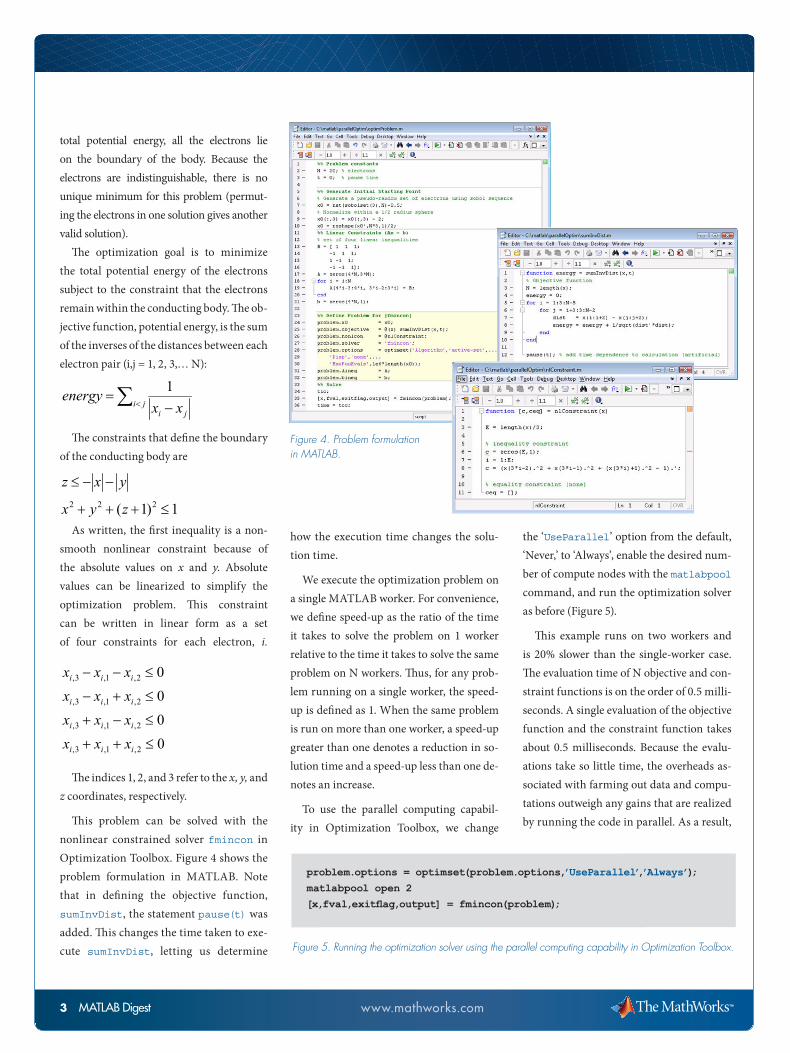
This problem can be solved with the nonlinear constrained solver fmincon in Optimization Toolbox. Figure 4 shows the problem formulation in MATLAB. Note that in defining the objective function, sumInvDist, the statement pause(t) was added. This changes the time taken to exe-cute sumInvDist, letting us determine

how the execution time changes the solu-tion time.

We execute the optimization problem on a single MATLAB worker. For convenience, we define speed-up as the ratio of the time it takes to solve the problem on 1 worker relative to the time it takes to solve the same problem on N workers. Thus, for any prob-lem running on a single worker, the speed-up is defined as 1. When the same problem is run on more than one worker, a speed-up greater than one denotes a reduction in so-lution time and a speed-up less than one de-notes an increase.

To use the parallel computing capabil-ity in Optimization Toolbox, we change

the ‘UseParallel’ option from the default, ‘Never,’ to ‘Always’, enable the desired num-ber of compute nodes with the matlabpool command, and run the optimization solver as before (Figure 5).

This example runs on two workers and is 20% slower than the single-worker case. The evaluation time of N objective and con-straint functions is on the order of 0.5 milli-seconds. A single evaluation of the objective function and the constraint function takes about 0.5 milliseconds. Because the evalu-ations take so little time, the overheads as-sociated with farming out data and compu-tations outweigh any gains that are realized by running the code in parallel. As a result,

Figure 4. Problem formulation in MATLAB.

Figure 5. Running the optimization solver using the parallel computing capability in Optimization Toolbox.

problem.options = optimset(problem.options,’UseParallel’,’Always’);

matlabpool open 2

[x,fval,exitflag,output] = fmincon(problem);

∑< −=

jiji xx

energy 1

yxz −−≤

1)1( 222 ≤+++ zyx

0000

2,1,3,

2,1,3,

2,1,3,

2,1,3,

≤++

≤−+

≤+−

≤−−

iii

iii

iii

iii

xxxxxxxxxxxx


distributing computations to run in parallel is slower than running the problem serially.

This example shows that for optimiza-tion problems to benefit from running the computations in parallel, the cost associated with the function evaluations with gradient estimation must be greater than the overhead costs associated with data and code transfer.

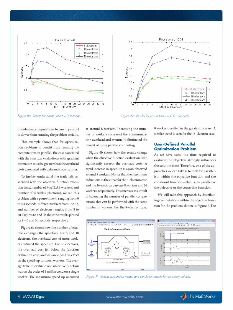
To further understand the trade-offs as-sociated with the objective function execu-tion time, number of MATLAB workers, and number of variables (electrons), we ran this problem with a pause time (t) ranging from 0 to 0.4 seconds, different workers from 1 to 32, and number of electrons ranging from 8 to 20. Figures 6a and 6b show the results plotted for t = 0 and 0.1 seconds, respectively.

Figure 6a shows how the number of elec-trons changes the speed-up. For 8 and 10 electrons, the overhead cost of more work-ers reduced the speed-up. For 16 electrons, the overhead cost fell below the function evaluation cost, and we saw a positive effect on the speed-up for most workers. The aver-age time to evaluate one objective function was on the order of 1 millisecond on a single worker. The maximum speed-up occurred

at around 8 workers. Increasing the num-ber of workers increased the communica-tion overhead and eventually eliminated the benefit of using parallel computing.

Figure 6b shows how the results change when the objective function evaluation time significantly exceeds the overhead costs. A rapid increase in speed-up is again observed around 8 workers. Notice that the maximum reductions in the curve for the 8-electron case and the 16-electron case are 8 workers and 16 workers, respectively. This increase is a result of balancing the number of parallel compu-tations that can be performed with the same number of workers. For the 8-electron case,

8 workers resulted in the greatest increase. A similar trend is seen for the 16-electron case.

User-Defined Parallel Optimization ProblemAs we have seen, the time required to evaluate the objective strongly influences the solution time. Therefore, one of the ap-proaches we can take is to look for parallel-ism within the objective function and the constraint function—that is, to parallelize the objective or the constraint function.

We will take this approach by distribut-ing computations within the objective func-tion for the problem shown in Figure 7. The

Figure 6b. Results for pause time t = 0.01 seconds.Figure 6a. Results for pause time t = 0 seconds.

Figure 7. Vehicle suspension model and simulation results for an empty vehicle.


goal of this problem is to design a suspen-sion system that minimizes the discomfort the driver would experience when traveling over a bump in the road. At the same time, we must account for uncertainty in the mass of the driver, passengers, and trunk load-ings. We can modify the four parameters that define the front and rear suspension system stiffness and damping rate: kf, kr, cf, cr. The masses of the driver, passengers, and trunk loadings are uncertain and have a normal distribution assigned to them.

A Monte-Carlo simulation is performed to capture the different vehicle loadings. The model outputs are angular acceleration about the center of gravity (thetadotdot, ··θ) and vertical acceleration (zdotdot, ··z).

The objective function, myCostFcnRR, contains a Monte-Carlo simulation used to evaluate the mean and standard deviation of acceleration that the passengers would experience (Figure 8). The goal is to mini-mize the mean and standard deviations.

In a Monte-Carlo simulation, each run is independent and therefore can benefit from parallel computation. To convert the problem from serial to parallel, we sim-ply replace the for loop construct with the parfor (parallel for loop) construct (Figure 9). The objective statements inside the parfor loop can then run in parallel,

speeding up the objective function evalu-ation time.

The optimization problem was run for three different values of nRuns, the num-ber of points to evaluate in the Monte-Carlo simulation. The results show that parallelizing the objective function yielded substantial performance gains (Figure 10).

Figure 8. Objective function used to run a Monte-Carlo simulation within the optimi-zation process.

Figure 9. Objective function modified to execute in parallel.

Figure 10. Results for the suspension system design problem.

Optimizer

Stop

Objective Function

Monte-Carlo Simulation

For k = 1 :N

Evaluate Model


For More Information

■ Designing for Reliability and Robustness. MATLAB Digest, January 2008 www.mathworks.com/company/robustdesign

■ Cleve’s Corner: Parallel MATLAB: Multiple Processors and Multiple Cores, The MathWorks News and Notes, June 2007. www.mathworks.com/company/ parallelmatlab

MATLAB Distributed Computing Server

Computer Setup

8 networked PCs configured with Linux 2.6, 2 dual-core AMD Opeteron 2.59 GHz

processors, 3 GB RAM.

91710v00 03/09

© 2009 The MathWorks, Inc. MATLAB and Simulink are registered trademarks of The MathWorks, Inc. See www.mathworks.com/trademarks for a list of additional trademarks. Other product or brand names may be trade-marks or registered trademarks of their respective holders.

Selecting a Parallelization MethodAs the results show, it is best to select a parallelization method based upon where computational expense is encoun-tered in the optimization problem. The first example showed that it is possible to see a reduction in performance even after distributing computations if the objective/constraint function execution time does not exceed the communication overhead. For the problem and hardware configuration tested, we would need an execution time of at least one millisec-ond to see any benefit from parallelizing the problem.

The second example showed that the benefits obtained by performing parallel computations can depend on the problem being solved. Using the parallelism within the objective function—that is, parallel-ising the objective function itself—result-ed in better performance than would have been possible using the parallel comput-ing option in Optimization Toolbox. In this example, the execution time of the objective function was the slowest part of the optimization problem, and speeding up the objective function resulted in the greatest reduction in solution time.

In summary, when selecting a parallel - i z ation approach it is important to consider the number of available workers and the execution time of the objective/constraint function relative to overheads associated

with distributing computations across multiple workers The built-in support in Optimization Toolbox is beneficial for problems that have objective/constraint functions with execution times greater than network overhead. However, parallel-izing the objective/constraint function it-self can be a better approach if it is the most expensive step in the optimization prob-lem and can be accelerated by parallelizing the objective function. ■

www.mathworks.com/company/robustdesign

www.mathworks.com/company/parallelmatlab

www.mathworks.com/company/parallelmatlab

Improving Optimization Performance with Parallel … MATLAB Digest Parallel computing techniques can...

Documents

Transcript of Improving Optimization Performance with Parallel … MATLAB Digest Parallel computing techniques can...