IMPROVING INTERACTIVE CLASSIFICATION

OF

SATELLITE IMAGE CONTENT

GOKHAN TEKKAYA

MAY 2007

IMPROVING INTERACTIVE CLASSIFICATION

OF

SATELLITE IMAGE CONTENT

A THESIS SUBMITTED TO

THE GRADUATE SCHOOL OF NATURAL AND APPLIED SCIENCES

OF

MIDDLE EAST TECHNICAL UNIVERSITY

BY

GOKHAN TEKKAYA

IN PARTIAL FULFILLMENT OF THE REQUIREMENTS

FOR

THE DEGREE OF MASTER OF SCIENCE

IN

COMPUTER ENGINEERING

MAY 2007

Approval of the Graduate School of Natural And Applied Sciences

Prof. Dr. Canan OZGEN

Director

I certify that this thesis satisfies all the requirements as a thesis for the degree of

Master Of Science.

Prof. Dr. Volkan ATALAY

Head of Department

This is to certify that we have read this thesis and that in our opinion it is fully

adequate, in scope and quality, as a thesis for the degree of Master Of Science.

Prof. Dr. Volkan ATALAY

Supervisor

Examining Committee Members

Prof. Dr. Nese Yalabık (METU,CENG)

Prof. Dr. Volkan Atalay (METU,CENG)

Asist. Prof. Dr. Selim Aksoy (Bilkent,CENG)

Asist. Prof. Dr. Tolga Can (METU,CENG)

Dr. Adem Mulayim (MilSOFT)

I hereby declare that all information in this document has been obtained and pre-

sented in accordance with academic rules and ethical conduct. I also declare that,

as required by these rules and conduct, I have fully cited and referenced all material

and results that are not original to this work.

Name, Lastname : Gokhan TEKKAYA

Signature :

iii

Abstract

IMPROVING INTERACTIVE CLASSIFICATION OF SATELLITE

IMAGE CONTENT

Tekkaya, Gokhan

M.Sc., Department of Computer Engineering

Supervisor: Prof. Dr. Volkan ATALAY

May 2007, 57 pages

Interactive classification is an attractive alternative and complementary for automatic

classification of satellite image content, since the subject is visual and there are not yet

powerful computational features corresponding to the sought visual features. In this

study, we improve our previous attempt by building a more stable software system

with better capabilities for interactive classification of the content of satellite images.

The system allows user to indicate a few number of image regions that contain a

specific geographical object, for example, a bridge, and to retrieve similar objects on

the same satellite images. Retrieval process is iterative in the sense that user guides

the classification procedure by interaction and visual observation of the results. The

classification procedure is based on one-class classification.

Keywords: One Class Classification, Satellite Image, SVDD, Interactive Classification

iv

Oz

UYDU GORUNTULERININ ETKILESIMLI

SINIFLANDIRMASININ IYILESTIRILMESI

Tekkaya, Gokhan

Yuksek Lisans, Bilgisayar Muhendisligi Bolumu

Tez Yoneticisi: Prof. Dr. Volkan ATALAY

Mayıs 2007, 57 sayfa

Etkilesimli sınıflandırma yontemi, konu gorsel oldugundan ve aranan gorsel oz nitelik-

ler ile ilgili hesaba dayalı etkili oz nitelikler bulunmadıgından, uydu goruntu iceriginin

otomatik sınıflandırılması yonteminin ilgi cekici bir alternatifi ve tamamlayacısıdır.

Bu calısmada onceki girisimimizi uydu goruntu iceriginin sınıflandırmasında daha

yetenekli olgun bir yazılım gerceklestirerek gelistiriyoruz. Sistem kullanıcının kopru

gibi belirli bir cografi nesneyi iceren az sayıda goruntu bolgesi belirtmesine ve ardından

aynı goruntuden benzer nesneler iceren bolgelere erismine olanak saglamaktadır.

Erisim sureci kullanıcının sınıflandırma islemini sonucları gorsel inceleyerek inter-

aktif bir sekilde yonlendirdigi tekrarlamalı bir surectir. Sınıflandırma islemi tek sınıf

sınııflandırma yontemine dayanmaktadır.

Anahtar Kelimeler: Tek Sınıf Sınıflandırma, Uydu Gorutu Icerigi, SVDD, Etkilesimli

sınıflandırma

v

To my family, friends and my beloved Ezgi

vi

Acknowledgments

I would like to express my sincere gratitude to my supervisor Prof. Dr. Volkan ATA-

LAY, without whose guidance and support this work could not be accomplished.

I deeply thank the members of the Department of Computer Engineering and my

friends for their suggestions during the period of writing the thesis.

I deeply thank my family for their understanding and their support.

vii

Table of Contents

Plagiarism . . . . . . . . . . . . . . . . . . . . . . . . . . . . . . . . . . . . . . . . . . . . . . . . . . . . . . . . . . . . iii

Abstract . . . . . . . . . . . . . . . . . . . . . . . . . . . . . . . . . . . . . . . . . . . . . . . . . . . . . . . . . . . . . . iv

Oz . . . . . . . . . . . . . . . . . . . . . . . . . . . . . . . . . . . . . . . . . . . . . . . . . . . . . . . . . . . . . . . . . . . . . . v

Acknowledgments . . . . . . . . . . . . . . . . . . . . . . . . . . . . . . . . . . . . . . . . . . . . . . . . . . . vii

Table of Contents . . . . . . . . . . . . . . . . . . . . . . . . . . . . . . . . . . . . . . . . . . . . . . . . . . . viii

List of Tables . . . . . . . . . . . . . . . . . . . . . . . . . . . . . . . . . . . . . . . . . . . . . . . . . . . . . . . . x

List of Figures . . . . . . . . . . . . . . . . . . . . . . . . . . . . . . . . . . . . . . . . . . . . . . . . . . . . . . . xi

List of Algorithms . . . . . . . . . . . . . . . . . . . . . . . . . . . . . . . . . . . . . . . . . . . . . . . . . . xiii

CHAPTER

1 Introduction . . . . . . . . . . . . . . . . . . . . . . . . . . . . . . . . . . . . . . . . . . . . . . . . . . . . . . 1

1.1 Problem Definition . . . . . . . . . . . . . . . . . . . . . . . . . . . . . 1

1.2 Motivation . . . . . . . . . . . . . . . . . . . . . . . . . . . . . . . . . 2

1.3 Achievements . . . . . . . . . . . . . . . . . . . . . . . . . . . . . . . . 3

1.4 Organization . . . . . . . . . . . . . . . . . . . . . . . . . . . . . . . . 4

2 Background Information on Classification And Feature Ex-

traction . . . . . . . . . . . . . . . . . . . . . . . . . . . . . . . . . . . . . . . . . . . . . . . . . . . . . . . . . . . 5

viii

2.1 Feature Extraction . . . . . . . . . . . . . . . . . . . . . . . . . . . . . 5

2.1.1 Spectral Features . . . . . . . . . . . . . . . . . . . . . . . . . . 5

2.1.2 Linear Features . . . . . . . . . . . . . . . . . . . . . . . . . . . 6

2.2 Classification Algorithms . . . . . . . . . . . . . . . . . . . . . . . . . 8

2.2.1 One Class Classification . . . . . . . . . . . . . . . . . . . . . . 8

2.2.2 Binary Classification . . . . . . . . . . . . . . . . . . . . . . . . 12

2.2.3 One-Class Classification Methods Used In This Study . . . . . 13

3 Interactive Classification System Software . . . . . . . . . . . . . . . . . 19

3.1 Software Design and Development Environment . . . . . . . . . . . . . 19

3.2 Software Description . . . . . . . . . . . . . . . . . . . . . . . . . . . . 23

4 Experiments And Results . . . . . . . . . . . . . . . . . . . . . . . . . . . . . . . . . . . . . . . . 26

4.1 Description of The System . . . . . . . . . . . . . . . . . . . . . . . . . 26

4.2 Prototype Design and Experiment . . . . . . . . . . . . . . . . . . . . 27

4.3 Comments On Experiment Results . . . . . . . . . . . . . . . . . . . . 50

4.3.1 Urban Area Experiment . . . . . . . . . . . . . . . . . . . . . . 50

4.3.2 Road Experiment . . . . . . . . . . . . . . . . . . . . . . . . . . 51

4.4 Comparison With Passive Learning . . . . . . . . . . . . . . . . . . . . 52

5 Conclusion . . . . . . . . . . . . . . . . . . . . . . . . . . . . . . . . . . . . . . . . . . . . . . . . . . . . . . . . . 54

References . . . . . . . . . . . . . . . . . . . . . . . . . . . . . . . . . . . . . . . . . . . . . . . . . . . . . . . . . . . . 56

ix

List of Tables

4.1 Prototype experiment: markers for objects used on experiment image. 31

4.2 Prototype experiment 1: SVDD parameters in urban area experiment

iterations. . . . . . . . . . . . . . . . . . . . . . . . . . . . . . . . . . . 33

4.3 Prototype experiment 1: Parzen density estimation parameters in ur-

ban area experiment iterations. . . . . . . . . . . . . . . . . . . . . . . 33

4.4 Prototype experiment 2: SVDD parameters in road experiment itera-

tions. . . . . . . . . . . . . . . . . . . . . . . . . . . . . . . . . . . . . . 33

4.5 Prototype experiment 2: SVM parameters in road experiment iterations. 34

4.6 Prototype experiment 1: SVDD performance observed in urban area

experiment iterations. . . . . . . . . . . . . . . . . . . . . . . . . . . . 34

4.7 Prototype experiment 1: Parzen density estimation performance ob-

served in urban area experiment iterations. . . . . . . . . . . . . . . . 34

4.8 Prototype experiment 2: SVDD performance observed in road exper-

iment iterations. . . . . . . . . . . . . . . . . . . . . . . . . . . . . . . 35

4.9 Prototype experiment 2: SVM performance observed in road experi-

ment iterations. . . . . . . . . . . . . . . . . . . . . . . . . . . . . . . . 35

4.10 SVM classifier performance observed with randomly generated training

sets. . . . . . . . . . . . . . . . . . . . . . . . . . . . . . . . . . . . . . 53

x

List of Figures

1.1 Overview of two phase classification approach. . . . . . . . . . . . . . 2

1.2 Overview of our system for finding region of interests. . . . . . . . . . 4

2.1 Regions in classification: a spherical data description boundary is

trained around a banana shaped target distribution. . . . . . . . . . . 9

2.2 Maximum-margin hyperplanes for a SVM trained with samples from

two classes. Samples along the hyperplanes are called the support

vectors. . . . . . . . . . . . . . . . . . . . . . . . . . . . . . . . . . . . 13

2.3 Spherical data description: hypersphere containing the target data is

described by the center a and radius R. Three objects are on the

boundary which are the support vectors. One object xi is outside and

has ξi > 0. . . . . . . . . . . . . . . . . . . . . . . . . . . . . . . . . . . 14

2.4 Impact of different width parameters values on a data description

trained on a banana-shaped set. Support vectors are marked by circles. 17

4.1 Prototype experiment image: single band SPOT panchromatic image

of size (2400×4000) with a spatial resolution of 10m. . . . . . . . . . . 29

4.2 Prototype experiment image: single band SPOT panchromatic image

of size (2400×1200) with a spatial resolution of 10m. . . . . . . . . . . 30

4.3 Initial training set for urban area experiment (Prototype experiment

1) containing 10 target objects. . . . . . . . . . . . . . . . . . . . . . . 35

4.4 Targets corrected by the user at the end of the first iteration of ur-

ban area experiment (Prototype experiment 1). Corrected targets are

added to the training set. . . . . . . . . . . . . . . . . . . . . . . . . . 36

xi

4.5 Outliers corrected by the user at the end of the first iteration of ur-

ban area experiment (Prototype experiment 1). Corrected outliers are

added to the training set. . . . . . . . . . . . . . . . . . . . . . . . . . 36

4.6 Initial training set for road experiment (Prototype experiment 2) con-

taining 10 target objects. . . . . . . . . . . . . . . . . . . . . . . . . . 36

4.7 Targets corrected by the user at the end of the first iteration of road

experiment (Prototype experiment 2). Corrected targets are added to

the training set. . . . . . . . . . . . . . . . . . . . . . . . . . . . . . . . 37

4.8 Outliers corrected by the user at the end of the first iteration of road

experiment (Prototype experiment 2). Corrected outliers are added to

the training set. . . . . . . . . . . . . . . . . . . . . . . . . . . . . . . . 37

4.11 SVDD classifiers, formed in iterations of urban area experiment (Pro-

totype experiment 1), shown in feature space. Outliers marked with

+ and targets with ∗. . . . . . . . . . . . . . . . . . . . . . . . . . . . 42

4.12 Parzen density estimation classifiers, formed in iterations of urban area

experiment (Prototype experiment 1), shown in feature space. Outliers

marked with + and targets with ∗. . . . . . . . . . . . . . . . . . . . . 43

4.15 Classification results, obtained with SVDD in road experiment (Pro-

totype experiment 2), shown in scaled feature space. Outliers marked

with � and targets with o. . . . . . . . . . . . . . . . . . . . . . . . . . 48

4.16 Classification results, obtained with SVM in road experiment (Proto-

type experiment 2), shown in scaled feature space. Outliers marked

with � and targets with o. . . . . . . . . . . . . . . . . . . . . . . . . . 49

xii

List of Algorithms

1 Canny Edge Detection . . . . . . . . . . . . . . . . . . . . . . . . . . . 6

2 Connected Component Labelling . . . . . . . . . . . . . . . . . . . . . 7

3 Iterative End-point Fitting . . . . . . . . . . . . . . . . . . . . . . . . 7

4 Classification Using Spectral Features . . . . . . . . . . . . . . . . . . 30

5 Classification Using Linear Features . . . . . . . . . . . . . . . . . . . 31

xiii

Chapter 1

Introduction

1.1 Problem Definition

Today, world’s highest resolution commercial satellite GeoEye-1 has a spatial reso-

lution of 41cm in collecting panchromatic images and it is known that spy satellites

have even better resolutions. With that much information, satellite images have

many applications in agriculture, geology, forestry, regional planning, education, in-

telligence and warfare. However, with the increase in resolution, the amount of data

to be handled accumulates. Therefore, extracting data and then exploration are

becoming challenging problems in remote sensing applications. To cope with the

increasing amount of data, a two phase approach, which is proposed in Oral Dalay’s

thesis [3] is given in Figure 1.1. The aim is to find regions of interest in first phase

so as to perform more refined analysis on these regions of interest. In this study,

we focus on the first phase, and one of the alternative approaches in the analysis of

such large images is to profit from user interaction. For this purpose we designed

an interactive classification software, which is based on active learning principles, to

detect man made (structural) geographical objects. User starts with a small set of

sample images, containing sought geographical object, and refines incrementally the

classification performance by interaction.

1

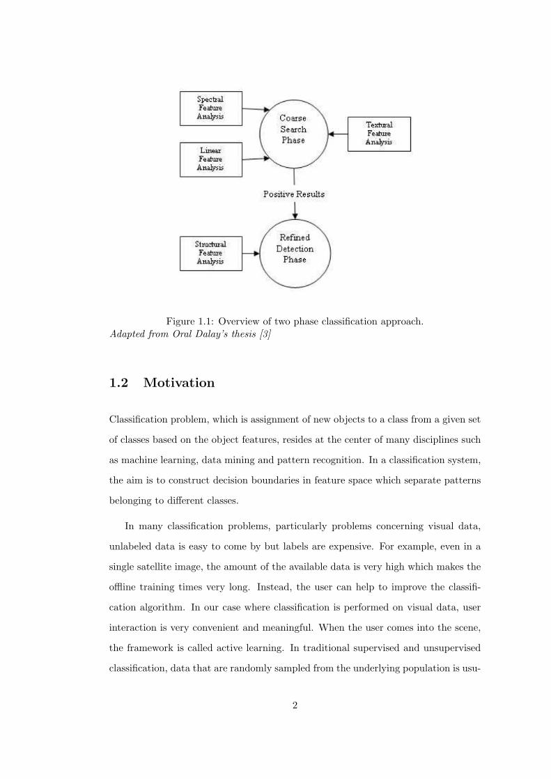
Figure 1.1: Overview of two phase classification approach.Adapted from Oral Dalay’s thesis [3]

1.2 Motivation

Classification problem, which is assignment of new objects to a class from a given set

of classes based on the object features, resides at the center of many disciplines such

as machine learning, data mining and pattern recognition. In a classification system,

the aim is to construct decision boundaries in feature space which separate patterns

belonging to different classes.

In many classification problems, particularly problems concerning visual data,

unlabeled data is easy to come by but labels are expensive. For example, even in a

single satellite image, the amount of the available data is very high which makes the

offline training times very long. Instead, the user can help to improve the classifi-

cation algorithm. In our case where classification is performed on visual data, user

interaction is very convenient and meaningful. When the user comes into the scene,

the framework is called active learning. In traditional supervised and unsupervised

classification, data that are randomly sampled from the underlying population is usu-

2

ally gathered and then a classifier or a model is induced. This methodology is called

passive learning. A passive learner receives a random data set from the world and

then outputs a classifier or model. On the other hand, in active learning, user se-

lects the examples hopefully in an intelligent manner in order to reduce the required

labeling effort while retaining the accuracy. This framework would allow the user

the flexibility to choose the data points that s/he feels which are most relevant for

classification. Besides, since in our case the data is visual, the algorithm may query

the user for the labels of the selected examples.

In our system, only detection of objects belonging to one class (the target class),

which is sampled by the user, is required. In most cases, there will be a large imbal-

ance between the target class and all other classes (the outliers) and it is very hard to

get a complete set of examples for the outliers. For this, we use classifiers which are

especially constructed for this type of problem: one-class classifiers. These classifiers

aim at describing the target class and distinguish that from all other possible objects.

These one-class classifiers are constructed such that they only require examples of

the target class.

1.3 Achievements

We are interested in applying active learning principles for analysis of panchromatic

satellite images. For this purpose, we have focused on the first phase of the interactive

classification system whose overview is given in Figure 1.1. We have proposed a new

approach based on one-class classifiers. Since it is necessary to prove the concept

approach, a prototype has been implemented before starting the design of the final

system. The overview of the proposed system is given in Figure 1.2.

The main idea behind the system is to get user feedback and iteratively improve

the performance of the classifier. First step in the classification process is the gener-

ation of the initial training set of sample regions containing example target objects,

3

by the user. Features from these regions are computed and then the result of the

classification is presented to the user. From this point, user can eliminate some of

the wrongly detected targets and perform classification again in an iterative manner.

The two most important issues in our system are given below.

• It is an example of active learning approach.

• It is based on one-class classification problem, i.e. only examples of target class

are available and an object is labeled as target or outlier.

Figure 1.2: Overview of our system for finding region of interests.

1.4 Organization

The organization of this thesis is as follows. In Chapter 2 background information

on techniques used in this study is given. Details of interactive classification system

is described in Chapter 3. The prototype and the proposed system are evaluated

in Chapter 4. The proposed system is discussed in Chapter 5, which concludes the

thesis.

4

Chapter 2

Background Information on

Classification And Feature

Extraction

In this chapter, we focus on and give detailed information about methods and algo-

rithms used throughout our study.

2.1 Feature Extraction

2.1.1 Spectral Features

In order to deal with urban areas in panchromatic satellite images, we first follow the

traditional approach where mean and standard deviation of pixel gray values in the

regions with fixed same size, which form the image are employed. The mean µ and

standard deviation σ of pixel gray values of the regions are computed as follows.

µ =1N

N∑i=1

xi (2.1)

5

σ = 2

√√√√ 1N

N∑i=1

(xi − µ)2 (2.2)

where xi indicates gray value of pixel i and N is total number of pixels in the region.

2.1.2 Linear Features

In satellite images, man-made objects such as roads, buildings may be discriminated

based on linear features. In this study, we apply the same linear feature extraction

method as presented in Oral Dalay’s thesis study [3]. Steps of linear feature extraction

are given below.

Step 1 Canny Edge Detection: Binary edge image is computed using Canny edge

detection algorithm [1] presented in Algorithm 1.

Algorithm 1 Canny Edge Detection1: Convolve Image I with a Gaussian of scale σ2: for all pixels p in I do3: Find edge magnitude and edge direction using Sobel operator4: end for5: for each pixel p with non-zero edge magnitude do6: inspect two adjacent pixels along the edge direction7: if edge magnitude of one these is greater than edge magnitude of p then8: mark edge pixel p for deletion9: end if

10: end for11: Apply hysteresis thresholding with t low and thigh

Step 2 Connected Component Labeling: Boundary curves are formed by ap-

plying the connected component algorithm [9] to binary edge image. Connected

component labeling algorithm is shown in Algorithm 2.

6

Algorithm 2 Connected Component LabellingRequire: binary edge Image I1: for all pixels p in I do2: if p == 1 then3: if all of four neighbor pixels (top, left, top-left and top-right) == 0 then4: assign a new label to p5: else if only one neighbor == 1 then6: assign neighbor’s label to p7: else8: assign one of the neighbors’ label to p and make a note of equivalences9: end if

10: end if11: end for12: Assign a unique label for each equivalence class13: for all pixels p in I do14: if p has a label then15: replace its label by the label assigned to its equivalence class16: end if17: end for

Step 3 Boundary Curve Segmentation by Polynomial Approximation: Linear

segments are formed by applying the iterative end-point fit algorithm [4] given

in Algorithm 3, and a non-uniform ten level histogram of the length of these

line segments is computed as linear features.

Algorithm 3 Iterative End-point Fitting1: Extract Edge Image with connected components computed2: for all connected components in edge Image do3: repeat4: connect the start and end points of the connected component with a line L5: Detect edge pixel P of the component with the maximum distance d to L6: if d < threshold then7: break8: else9: Split component at P into S1 and S2 and for both subsets goto 3

10: end if11: until all subsets have been checked12: merge collinear points13: end for

7

2.2 Classification Algorithms

Classification of a new object as target or outlier may be performed in two different

ways. The first one is the classical n-class classification, while the other is one-class

classification. In an n-class classification problem, a new object is assigned to one of a

set of n known classes. On the other hand, in a one-class classification problem, only

one class (target) is known and a new object is either assigned as target or outlier

(all classes other than target).

In this study, main interest about classification is on one-class classification meth-

ods. Classical n-class classification methods are only used in final iterations of the

classification process when using high dimensional features. Section 2.2.1 briefly

describes one-class classification and it is mainly based on David M. Tax’s the-

sis [15]. Section 2.2.2 briefly describes binary classification and Support Vector Ma-

chines(SVM) [17] that as used in this study.

2.2.1 One Class Classification

In one class classification method, a boundary is formed around given target objects

with the aim of maximizing target acceptance rate while minimizing the acceptance

of outlier objects. One-class classification methods can be analyzed in three groups:

• density estimation,

• boundary methods,

• reconstruction methods.

The most important feature of one-class classifiers is the tradeoff between false posi-

tives (outlier objects labeled by classifier a target) and false negatives (target objects

labeled by classifier as outlier). This can be visualized as in Figure 2.1. The enclosed

area labeled as XT is the target distribution. The circular data description is the

resulting area of a one-class classification method. The dark gray area labeled as

8

EII is the area of false positives and light gray area labeled as EI is the area of false

negatives. As it can be observed from Figure 2.1, a tradeoff between false positives

and false negatives cannot be avoided. Increasing the volume of the data description

to decrease the false negatives, will automatically increase the number of the false

positives. Therefore EII will increase.

Figure 2.1: Regions in classification: a spherical data description boundary is trainedaround a banana shaped target distribution.Adapted from David M. Tax’s thesis [15]

2.2.1.1 Features of One-Class Classification Approaches

While comparing different one-class classification approaches, not only the errors are

important, but also the following features.

Robustness to outliers: For training one class classification methods, a set which

is a characteristic representation for the target distribution should be used.

However, this training set may already happen to contain some outliers. A one-

class classification method should reject these outliers while trying to accept

the target class objects as much as possible.

9

Incorporation of known outliers: Available outliers in training set can be used

to tighten the boundary around the target class. The model of the target set

and the training procedure allow the usage of outlier objects for more precise

classification. For example, when the target set is modeled with one Gaus-

sian distribution, outlier objects cannot be used, while other methods such as

Parzen [5] density estimation and support vector data description (SVDD) can

use this information.

Magic parameters and ease of configuration: From the users’ point of view,

the number of free parameters whose values have to be determined is one of

most important features of any method. These parameters are called the magic

‘parameters, because they often have a big influence on the final performance

and no clear rules are given how to set them. Since our system is an interactive

one, a method with minimum number of magic parameters is more suitable to

use.

Computation and storage requirements: A last criterion to consider is the com-

putational requirements of the methods. This criterion is also very important,

since in our system, training is performed on-line and the classification method

is adaptively changed by the inputs from the user.

2.2.1.2 Density Methods

Estimating the density of the target class distribution using training data is the most

straightforward method to obtain a one-class classifier. A classifier is formed by set-

ting a threshold on this density estimation. Density estimation methods produces

good results when the sample size is sufficiently high and a flexible density model

is used; for example a Parzen density estimation. Unfortunately, density estima-

tion methods require a large number of training samples to overcome the curse of

dimensionality; that is the volume that should be described by classifier increases

exponentially as the number of features increases [5]. Examples for density methods

10

are:

• Gaussian,

• mixture of Gaussians,

• Parzen density estimation.

2.2.1.3 Boundary Methods

In boundary methods, a closed boundary around the target set is optimized. Even

the volume is not always actively minimized, most boundary methods have a strong

bias towards a solution having minimal volume. The size of the volume depends on

the fit of the model to the data. In most cases, distances or weighted distances to an

edited set of objects in the training set are computed. Since the distance calculation

is sensitive to scaling, boundary methods, heavily relying on the distances between

objects, are sensitive to the scaling of features used in classification. If we want to

compare density methods with boundary methods in terms of the size of the training

set required, is smaller in boundary methods. Examples for boundary methods are:

• k-centers,

• d nearest neighborhood (NN-d),

• support vector data description (SVDD).

2.2.1.4 Reconstruction Methods

In reconstruction methods, a model is fitted to the data by using prior knowledge

about the data and making assumptions about the generating process. New objects

can then be described in terms of a state of the generating model. We assume

that a more compact representation of the target data can be obtained and that in

this encoded data the noise contribution is decreased. Most of these methods make

11

assumptions about the clustering characteristics of the data or their distribution in

subspaces. A set of prototypes or subspaces is defined and a reconstruction error is

minimized. Examples for reconstruction methods are:

• k-means clustering,

• self-organizing maps,

• auto-encoder networks.

The above methods differ in the definition of the prototypes or subspaces, their

reconstruction error and their optimization routine.

2.2.2 Binary Classification

Binary classification is an example of n-class classification where data belongs to one

of the two classes, which are available for training. In this study we use Support

Vector Machines (SVM) as a binary classification method.

2.2.2.1 Support Vector Machines

Support Vector Machines are learning machines that can perform binary classification

tasks. The main idea behind the SVM is that, it maps input vectors xi to a higher

dimensional space and constructs a maximal separating hyperplane. Two parallel

hyperplanes are constructed on each side of the hyperplane that separates the data.

The separating hyperplane is the hyperplane that maximizes the distance between

the two parallel hyperplanes as shown in Figure 2.2. An assumption is made that

the larger the margin or distance between these parallel hyperplanes the better the

generalization error of the classifier will be.

12

Figure 2.2: Maximum-margin hyperplanes for a SVM trained with samples from twoclasses. Samples along the hyperplanes are called the support vectors.

2.2.3 One-Class Classification Methods Used In This Study

In order to decide which methods to use in this study, we consider the features

described in Section 2.2.1.1. In this work, we use one boundary method, SVDD and

one density estimation method, Parzen, since both methods are robust to outlier

objects in training data and they are able to incorporate outliers to tighten the

boundary of the target class. In addition, both methods have only one free parameter

which has to be set by the user and their computational power requirements can be

handled by current processors adequately for an interactive system. One of the

reasons for using two different methods is their performances with respect to the

properties of training data. SVDD is more suitable where training data set contains

a-typical samples, while Parzen density estimation produces better results with a

representative training data set. Here, more information about SVDD and Parzen

density estimation are given.

13

2.2.3.1 Support Vector Data Description (SVDD)

In SVDD method, a hypersphere is formed to contain all target objects and volume

of the hypersphere is minimized to reject maximum number of outliers.

Spherical data description is defined with a center a and a radius value R and all

target objects are required to be inside the sphere.

Figure 2.3: Spherical data description: hypersphere containing the target data isdescribed by the center a and radius R. Three objects are on the boundary whichare the support vectors. One object xi is outside and has ξi > 0.Adapted from David M. Tax’s thesis [15]

Structural error is defined as εstruct(R, a) = R2 with the minimization of the

constraint ‖ xi − a ‖2≤ R2, ∀i. To allow outliers in training of the classifier, it

is possible for objects xi to have a distance to the center a greater than R2. Since

those objects should be penalized, an empirical error is added to structural error

with the introduction of variable ξ,∀xi. The final error is defined as ε(R, a, ξ) =

R2 +C∑

i ξi and the free parameters a,R, ξ should be optimized with the constraint

‖ xi−a ‖2≤ R2 + ξi, ξi ≥ 0,∀i. This is done by using Lagrange multipliers and final

Lagrangian [14] is

L =∑

i

αi(xi · xi) −∑ij

αiαj(xi · xj) (2.3)

where αi is Lagrange multiplier and xi · xj is inner product between xi and xj .

14

Equation 2.3 is an instance of quadratic programming problem and several al-

gorithms exist for the solution of this problem [10]. A new object is labeled as

target when the distance to the hypersphere center is less than equal to the radius

R. Spherical data description enables incorporation of outlier objects in training and

it is identical to the one without outliers.

The hypersphere is a very tight model of the boundary of the data and in real life

problems it does not fit the data well. To overcome this problem Kernel trick [17]

can be utilized in which the data is mapped to a new representation in order to

obtain a better fit between the actual data boundary and the hypersphere model.

Assume we are given a mapping Φ(x) of the data which improves this fit: x∗ = Φ(x).

Equation 2.3 becomes

L =∑

i

αiΦ(xi) · Φ(xi) −∑ij

αiαjΦ(xi) · Φ(xj) (2.4)

where αi is Lagrange multiplier and Φ(xi) ·Φ(xj) is inner product between Φ(xi) and

Φ(xj).

In Equation 2.4, all mappings Φ(x) present only in inner products with other

mappings. It is possible to define a new function of two input variables, called a

kernel function: K(xi, xj) = Φ(xi) ·Φ(xj) and replace all occurrences of Φ(xi) ·Φ(xj)

by this kernel. This results in:

L =∑

i

αiK(xi, xi) −∑ij

αiαjK(xi, xj) (2.5)

where αi is Lagrange multiplier and K is kernel function.

A good kernel function, which maps the target data onto a bounded, spherically

shaped area in the feature space and outlier objects outside this area should be

defined. In this case, the hypersphere model fits the data well and good classification

performance is obtained.

15

In this study, we use a flexible data description with Gaussian kernel:

K(xi, xi) = exp(‖ xi − xj ‖2

s2

)

Since K(xi, xj) = 1, both the Lagrangian and the evaluation function simplify. Ig-

noring constants Equation 2.5 becomes:

L = −∑ij

αiαjK(xi, xj) (2.6)

From the solution of Equation 2.6, a new object z is labeled as target when Equa-

tion 2.7 is true. ∑i

αi exp(− ‖ z − xi ‖2

s2

)>

12(B −R2) (2.7)

where αi is Lagrange multiplier and B = 1 +∑

ij αiαjK(xi, xj).

Note that B only depends on the support vectors xi (not on the object z) and

Equation 2.7 is a thresholded mixture of Gaussians.

The character of the data description depends on the value of the width parameter

s. For very small values of s, differences between K(xi, xj) for different i and j can

be ignored, and the total model becomes a sum of equally weighted Gaussians, which

is identical to a Parzen density estimation with a small width parameter. For very

large values of s, values near or large than the maximum distance between objects,

the flexible data description becomes the original spherical data description. For

intermediate values of s, the data description of forms a weighted Parzen density. In

Figure 2.4, on the left a small s = 1.0 width parameter is used, and on the right a

large s = 25.0 is used (average nearest neighbor distance between the target objects

is 1.1). In all cases, except when s becomes considerably large than the average

distance, the description is tighter than the original spherical data description. Note

that with increasing s the number of support vectors decreases.

16

Figure 2.4: Impact of different width parameters values on a data description trainedon a banana-shaped set. Support vectors are marked by circles.Adapted from David M. Tax’s thesis [15]

2.2.3.2 Parzen Density Estimation

The estimated density is a mixture of Gaussian kernels centered on the individual

training objects, with diagonal covariance matrices∑

i = hI

pp(x) =1

n

∑i

pN(x; xi, hI) (2.8)

where pN is Gaussian kernel, h is the kernel width parameter I is the identity matrix,

n is the size of training set.

In Equation 2.8, kernel width h is equal in each feature direction meaning that the

Parzen density estimator assumes equally weighted features and so it will be sensitive

to the scaling of the feature values of the data, especially for lower sample sizes.

The only free parameter to train a Parzen density estimation is the optimal width

of the kernel h, which is optimized using the maximum likelihood [11] on the training

data set using leave-one-out. A good description totally depends on the representa-

tiveness of the training set i.e. a bad training set most probably results in a classifier

with poor performance. The computational cost for training a Parzen density es-

timator is almost zero, but the test is expensive. All training objects have to be

stored and, during test, distances to all training objects have to be calculated and

17

sorted. This might severely limit the applicability of the method, especially when

large datasets in high dimensional feature spaces are considered.

18

Chapter 3

Interactive Classification

System Software

The software is mainly an integration of classification, feature extraction and visual-

ization methods provided to the user for detecting geographical objects quickly and

precisely in satellite images.

3.1 Software Design and Development Environment

Before the implementation phase several design decisions are taken and they are

stated below.

• Software should be open-source, and well documented for enabling potential

contribution.

• Software should be cross-platform and run on at least Linux and Windows

operating systems.

• Software should have an open architecture to allow addition of new classification

and feature extraction methods.

19

In order to conform to the design decisions, cross platform graphical user interface

(GUI) library wxWidgets written in C++ is used. For code generation gcc is used on a

Windows platform with the help of MinGW (Minimalist GNU for Windows). Eclipse

is used as integrated development environment (IDE) since it can run on aimed

platforms. With these development environment set, software can be maintained

easily either on Windows or Linux platforms.

In this study, to develop an extendible software, an open architecture is employed.

The architecture of the software is based on well-known design patterns. A general

repeatable solution to commonly faced problems in software design is called a design

pattern [6]. A design pattern is not a finished design that can be transformed directly

into code. It is a description or template for how to solve a problem that can be used in

many different situations. Design patterns can speed up the development process by

providing tested, proven development paradigms. Effective software design requires

considering issues that may not become visible until later in the implementation.

Reusing design patterns helps to prevent subtle issues that can cause major problems

and improves code readability for coders and architects familiar with the patterns.

Design patterns can be classified in terms of the underlying problem they solve.

Examples of problem-based pattern classifications include:

• Fundamental patterns,

• Creational patterns, which deal with the creation of objects,

• Structural patterns, which ease the design by identifying a simple way to realize

relationships between entities,

• Behavioral patterns, which identify common communication patterns between

objects and realize these patterns.

As a fundamental principle of object oriented design, interface pattern is used

thoroughly. As seen from the class design of the software in Figure 3.1a and Fig-

ure 3.1b, classification, feature extraction classes are based on interface classes. From

20

creational patterns, Factory [8] pattern is employed for creation of specific imple-

mentations (SVDD, Parzen density estimation, SVM)of these interfaces. With this

design decision, graphical user interface (GUI) classes have no direct connection to

the specific implementations of IClassifier and IFeatureComputer interfaces. Fac-

tory classes FeatureComputerFactory, ClassifierFactory provide implicit access to

the functions of the implementation classes. For the GUI architecture, Model-View-

Presenter (MVP) [12] architectural pattern is employed, which proposes logic free

view classes controlled by presenter classes through view interfaces. This will help

the developer easily to change the view classes or even the GUI library without any

modification to the presenter classes, which contain the logical code.

(a) Classifier Class Design

21

(b) Graphical User Interface Class Design

Figure 3.1: Class design of the interactive classification system software.

22

3.2 Software Description

For the demonstration of the ideas of this study, we implemented an interactive clas-

sification software. GUI parts of the software was developed using wxWidgets [13]

framework with C++ programming language. Dockable GUI elements from wxWid-

gets framework were employed in order to provide an easily customizable interface

for users as shown in Figure 3.2. One class classification and feature computation

algorithms were implemented with Matlab using ddtools [16], prtools [7] and inte-

grated to the software through Matlab C external interface libraries. Code parts,

which are interacting with the Matlab, were hidden in one class classifier implemen-

tations, hence Matlab dependency was minimized. Finally for binary classification

libsvm [2] was used in a similar way to usage of Matlab for one class classification.

Main functionalities provided by our classification software are given below.

• Several image formats including JPEG, BMP, PNG, GIF, PCX, TIF and XPM

are supported for processing.

• Algorithms for extracting spectral features and linear features described in Sec-

tion 2.1.1 and Section 2.1.2, respectively are available.

• As one class classifiers, SVDD and Parzen density estimation are available in

addition to the SVM classifier, which can be used by the user as well.

• A half size overview image is displayed, for helping user to navigate through

large images easily. This overview and original size image is linked together,

such that whenever user selects a point in overview or original image view, the

other view is automatically scrolled to the selected point.

• A plot view is presented to the user for displaying features or multidimensional

scaled features (in case of high dimensional features). The plot view is also

linked to the original image view such that, whenever a point in feature space

is selected the original image is scrolled automatically to the region having the

feature which is closest to the selected point in feature space.

23

• The list of target and outlier examples are displayed in separate views, which

are interactively managed by the user through the interface.

• Parameters of classifiers can be changed easily from the parameter views pro-

vided for each classifier.

• Classification results are shown in a separate layer on the overview image. In

addition, features from target and outlier objects are labeled differently in the

plot view when classification is performed.

• It is possible for user to save classification results or training set information

for resuming classification process in another time.

(a) Docked interface - dialogs

24

(b) Floating interface - dialogs

Figure 3.2: Interface of the interactive classification software.

25

Chapter 4

Experiments And Results

4.1 Description of The System

The main idea behind the system is to get user feedback and iteratively improve the

performance of the classifier. First step in the classification process is generation of

the initial set containing example target objects. This initial set contains only target

objects. The result of the classification is subsequently presented to the user with

nearest outliers highlighted. Nearest outliers to the target data description have the

most valuable information to tighten the boundary around the target distribution.

User adds more examples (target or outlier) to the training set and the target data

description is re-computed. This process is proceeded with the support vector data

description (SVDD) until a preset training set size is achieved or the user selects to

another classifier, Parzen density estimation or SVM. In the first iterations, SVDD is

preferred to Parzen density estimation and SVM, because the latter classifiers require

a larger training set than SVDD. In addition, Parzen density estimation and SVM

produce poor results in case of a bad representative training set, which is more likely

to happen in early iterations.

26

4.2 Prototype Design and Experiment

The prototype is an exact copy of the proposed interactive system except the graphi-

cal user interface (GUI) parts. User interaction is simulated by a series of predefined

labels given to image regions containing the target object and outlier objects. After

each iteration, size of the training set is increased and the classifier is re-run. The

boundary around the target data description and nearest outliers to the classifier

boundary is presented to the user for feedback. At the end of each iteration, classi-

fier performance is compared against the ground truth data existing with the example

satellite image.

The aim of the prototyping is to prove that the method will work as it is designed.

Therefore we decided to make two experiments; the first experiment is with simple

spectral features of intensity values while the second experiment is based on linear

features.

First experiment is aimed at detection of urban areas in a satellite image with

existing ground truth data. The satellite image given in Figure 4.1 is split into 1500

regions of size 80×80 pixels and 231 of these regions are labeled as urban area by an

expert. One of the reasons for using spectral features is that they are simple, easy to

calculate and produce good results for urban area targets in gray level images. Parzen

density estimation is preferred to SVM in this experiment, since the dimension of the

spectral features is just two.

Second experiment is aimed at proving that our approach produces good results,

in case of high dimensional feature space. Regions which contain main roads in satel-

lite image given in Figure 4.2 are to be detected. The image is split into 450 regions

and 127 of these regions are labeled as road by an expert. SVM is preferred to Parzen

density estimation in this experiment, since the latter requires a complete density es-

timate in complete feature space and in cases like this when high dimensional feature

spaces are present, this classifier requires huge amount of data.

27

The notations used in interactive classification algorithm of the prototype is given

as follows;

• I : input satellite image,

• µ : mean of an image region in I,

• σ : standard deviation of an image region in I,

• H : linear segment histogram of an image region in I,

• ω : classifier,

• Λ : set of all image regions in I,

• Λtrain : set of image regions in I used in training of ω.

28

Figure 4.1: Prototype experiment image: single band SPOT panchromatic image ofsize (2400×4000) with a spatial resolution of 10m.

29

Figure 4.2: Prototype experiment image: single band SPOT panchromatic image ofsize (2400×1200) with a spatial resolution of 10m.

The classification algorithms used, follows the approach given in Section 4.1. The

steps of the algorithms for urban area detection and road detection are given in

Algorithm 4 and Algorithm 5 respectively.

Algorithm 4 Classification Using Spectral Features1: for all image regions i in Λ do2: calculate µi and σi

3: end for4: set ω = SVDD5: get Λtrain from user6: repeat7: set ω parameters8: train ω with Λtrain

9: apply ω to Λ10: show I11: mark classified target objects on I12: mark Λtrain on I13: mark nearest outliers on I14: show ω performance against ground truth information15: user adds new target and outlier objects to Λtrain

16: if user request classifier change then17: ω = Parzen density estimation18: end if19: until user stops iteration

30

Algorithm 5 Classification Using Linear Features1: for all image regions i in Λ do2: calculate H3: end for4: set ω = SVDD5: get Λtrain from user6: repeat7: set ω parameters8: train ω with Λtrain

9: apply ω to Λ10: show I11: mark classified target objects on I12: mark Λtrain on I13: mark nearest outliers on I14: show ω performance against ground truth information15: user adds new target and outlier objects to Λtrain

16: if user request classifier change then17: ω = SVM18: end if19: until user stops iteration

The experiment for detecting urban areas consists of two runs of five iterations

with increasing training set size. At the end of the each iteration, the results are

presented visually on experiment image by using markers defined in Table 4.1 and

classifier boundary around the features is plotted.

The experiment for detecting areas containing roads consists of two runs of six

iterations with increasing training set size. At the end of the each iteration, the

results are presented visually on experiment image and multidimensional scaling is

performed for displaying results on scaled features. Since used linear features are ten

dimensional, classifier boundary cannot be plotted.

Table 4.1: Prototype experiment: markers for objects used on experiment image.Marker Definition Marker SymbolAll targets from ground truth data �Targets in training set +Outliers in training set +Detected targets xNearest outliers o

31

Performance of the classification is evaluated by the criteria defined below:

True positives: number of correctly detected targets

False positives: number of outliers detected as targets

True negatives: number of correctly detected outliers

False negatives: number of targets detected as outliers

Precision:true positives

true positives + false positives

Recall:true positives

true positives + false negatives

In the urban area experiment, for the first run SVDD is used with given training

set size and parameters in Table 4.2, and for the second run we use the training

set generated during the first run and Parzen density estimation with parameters

given in Table 4.3. Image regions in the initial training set are given in Figure 4.3.

Targets and outliers corrected by the user after first iteration are given in Figure 4.4

and Figure 4.5, respectively. Results for SVDD and Parzen density estimation on

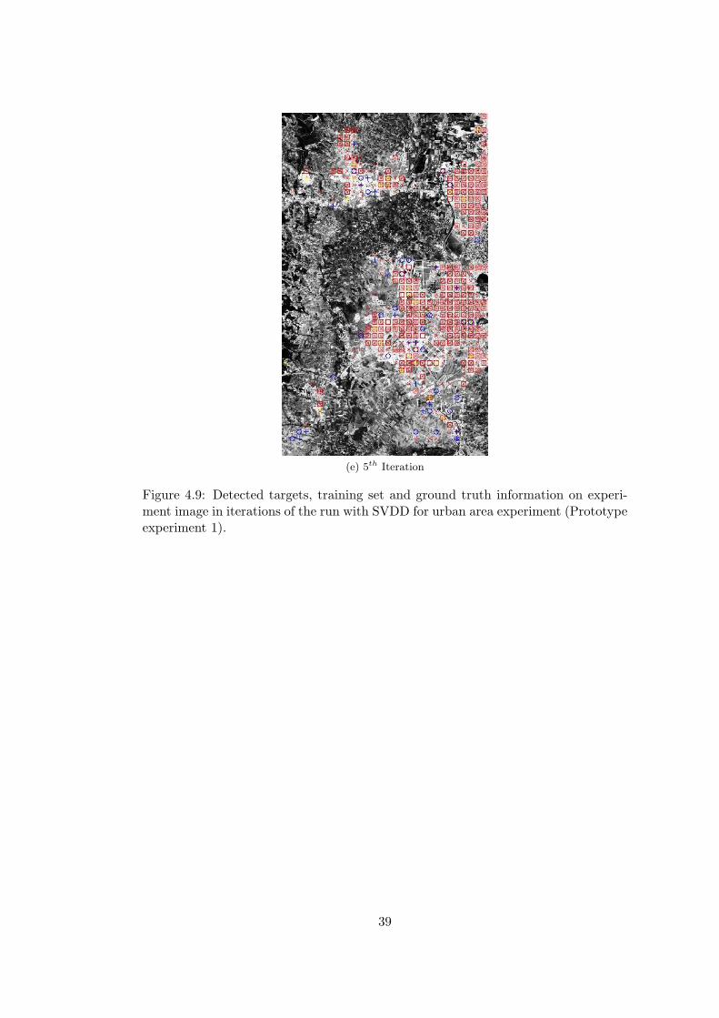
the experiment image are given in Figure 4.9 and Figure 4.10, respectively. Perfor-

mance of SVDD and Parzen density estimation can be visualized in Figure 4.11 and

Figure 4.12, respectively.

In the road experiment, for the first run SVDD is used with given training set

size and parameters in Table 4.4, and for the second run we use the training set

generated during the first run and SVM classifier with parameters given in Table 4.5.

Image regions in the initial training set are given in Figure 4.6. Targets and outliers

corrected by the user after first iteration are given in Figure 4.7 and Figure 4.8,

respectively. Results for SVDD and SVM classifiers on the experiment image are

given in Figure 4.13 and Figure 4.14, respectively. Performance of SVDD and SVM

classifiers can be visualized in Figure 4.15 and Figure 4.16, respectively.

32

Table 4.2: Prototype experiment 1: SVDD parameters in urban area experimentiterations.

Iterationnumber

Target rejectionrate

# of supportvectors

Kernelwidth

# of targetexamples

# of outlierexamples

1 0.1 3 1 10 02 0.1 9 0.9 18 53 0.1 11 0.6 23 104 0.1 18 0.5 27 145 0.1 27 0.51 30 20

Table 4.3: Prototype experiment 1: Parzen density estimation parameters in urbanarea experiment iterations.

Iterationnumber

Target rejectionrate

Width # of targetexamples

# of outlierexamples

1 0.1 0.060 10 02 0.1 0.107 18 53 0.15 0.094 23 104 0.15 0.085 27 145 0.15 0.086 30 20

Table 4.4: Prototype experiment 2: SVDD parameters in road experiment iterations.

Iterationnumber

Target rejectionrate

# of supportvectors

Kernelwidth

# of targetexamples

# of outlierexamples

1 0.1 4 0.6 10 02 0.1 14 1.4 22 73 0.1 19 0.9 32 174 0.1 28 0.8 42 225 0.05 26 0.8 54 226 0.05 32 0.8 67 34

33

Table 4.5: Prototype experiment 2: SVM parameters in road experiment iterations.Iterationnumber

Gamma C # of supportvectors

# of targetexamples

# of outlierexamples

1 8 128 0 10 02 8 128 20 22 73 8 128 30 32 174 8 128 35 42 225 8 128 38 54 226 8 128 62 67 34

Table 4.6: Prototype experiment 1: SVDD performance observed in urban areaexperiment iterations.

Iterationnumber

Truepositives

Falsepositives

Truenegatives

Falsenegatives

Precision Recall

1 173 105 1164 58 0.62 0.752 199 182 1087 32 0.49 0.863 213 124 1145 18 0.63 0.924 213 111 1158 18 0.66 0.925 211 100 1169 20 0.68 0.91

Table 4.7: Prototype experiment 1: Parzen density estimation performance observedin urban area experiment iterations.

Iterationnumber

Truepositives

Falsepositives

Truenegatives

Falsenegatives

Precision Recall

1 190 77 1192 41 0.71 0.822 226 239 1030 5 0.49 0.973 226 168 1101 5 0.57 0.984 225 190 1079 6 0.54 0.975 225 150 1119 6 0.60 0.97

In Parzen density estimation method, target rejection rate is used for finding the

required threshold to reject lowest given fraction of the targets in the training data

set. In addition, in SVDD target rejection rate together with the kernel width affects

the number of support vectors identifying the data description [15].

34

Table 4.8: Prototype experiment 2: SVDD performance observed in road experimentiterations.

Iterationnumber

Truepositives

Falsepositives

Truenegatives

Falsenegatives

Precision Recall

1 69 72 251 58 0.49 0.542 90 85 238 37 0.51 0.713 93 85 238 34 0.52 0.734 100 80 243 27 0.56 0.795 107 91 232 20 0.54 0.846 108 96 227 19 0.54 0.85

Table 4.9: Prototype experiment 2: SVM performance observed in road experimentiterations.

Iterationnumber

Truepositives

Falsepositives

Truenegatives

Falsenegatives

Precision Recall

1 127 323 0 0 0.28 1.002 101 93 230 26 0.52 0.803 110 120 203 17 0.48 0.874 109 107 216 18 0.50 0.865 115 126 197 12 0.48 0.906 116 77 246 11 0.60 0.91

(a) (b) (c) (d) (e)

(f) (g) (h) (i) (j)

Figure 4.3: Initial training set for urban area experiment (Prototype experiment 1)containing 10 target objects.

35

(a) (b) (c) (d)

(e) (f) (g) (h)

Figure 4.4: Targets corrected by the user at the end of the first iteration of urban areaexperiment (Prototype experiment 1). Corrected targets are added to the trainingset.

(a) (b) (c) (d) (e)

Figure 4.5: Outliers corrected by the user at the end of the first iteration of urban areaexperiment (Prototype experiment 1). Corrected outliers are added to the trainingset.

(a) (b) (c) (d) (e)

(f) (g) (h) (i) (j)

Figure 4.6: Initial training set for road experiment (Prototype experiment 2) con-taining 10 target objects.

36

(a) (b) (c) (d) (e) (f)

(g) (h) (i) (j) (k) (l)

Figure 4.7: Targets corrected by the user at the end of the first iteration of roadexperiment (Prototype experiment 2). Corrected targets are added to the trainingset.

(a) (b) (c) (d) (e)

(f) (g) (h) (i) (j)

Figure 4.8: Outliers corrected by the user at the end of the first iteration of roadexperiment (Prototype experiment 2). Corrected outliers are added to the trainingset.

37

(a) 1st Iteration (b) 2nd Iteration

(c) 3rd Iteration (d) 4th Iteration

38

(e) 5th Iteration

Figure 4.9: Detected targets, training set and ground truth information on experi-ment image in iterations of the run with SVDD for urban area experiment (Prototypeexperiment 1).

39

(a) 1st Iteration (b) 2nd Iteration

(c) 3rd Iteration (d) 4th Iteration

40

(e) 5th Iteration

Figure 4.10: Detected targets, training set and ground truth information on exper-iment image in iterations of the run with Parzen density estimation for urban areaexperiment (Prototype experiment 1).

41

(a) 1st Iteration (b) 2nd Iteration

(c) 3rd Iteration (d) 4th Iteration

(e) 5th Iteration

Figure 4.11: SVDD classifiers, formed in iterations of urban area experiment (Pro-totype experiment 1), shown in feature space. Outliers marked with + and targetswith ∗.

42

(a) 1st Iteration (b) 2nd Iteration

(c) 3rd Iteration (d) 4th Iteration

(e) 5th Iteration

Figure 4.12: Parzen density estimation classifiers, formed in iterations of urban areaexperiment (Prototype experiment 1), shown in feature space. Outliers marked with+ and targets with ∗.

43

(a) 1st Iteration

(b) 2nd Iteration

(c) 3rd Iteration

44

(d) 4th Iteration

(e) 5th Iteration

(f) 6th Iteration

Figure 4.13: Detected targets, training set and ground truth information on exper-iment image in iterations of the run with SVDD for road experiment (Prototypeexperiment 2).

45

(a) 1st Iteration

(b) 2nd Iteration

(c) 3rd Iteration

46

(d) 4th Iteration

(e) 5th Iteration

(f) 6th Iteration

Figure 4.14: Detected targets, training set and ground truth information on ex-periment image in iterations of the run with SVM for road experiment (Prototypeexperiment 2).

47

(a) 1st Iteration (b) 2nd Iteration

(c) 3rd Iteration (d) 4th Iteration

(e) 5th Iteration (f) 6th Iteration

Figure 4.15: Classification results, obtained with SVDD in road experiment (Pro-totype experiment 2), shown in scaled feature space. Outliers marked with � andtargets with o.

48

(a) 1st Iteration (b) 2nd Iteration

(c) 3rd Iteration (d) 4th Iteration

(e) 5th Iteration (f) 6th Iteration

Figure 4.16: Classification results, obtained with SVM in road experiment (Prototypeexperiment 2), shown in scaled feature space. Outliers marked with � and targetswith o.

49

4.3 Comments On Experiment Results

In both of the performed experiments, we expect to have a steady improvement on

the precision and recall values at each iteration, since the size of the training sets are

increasing. In addition, we expect to have better results with SVDD compared to

Parzen density estimation and SVM in early iterations, since the latter two classifiers

require larger training sets to produce results close to that of produced by SVDD.

Also, we expect Parzen density estimation and SVM to produce better recall results

when the size of the training sets becomes larger, which occur only in final iterations.

4.3.1 Urban Area Experiment

Performance of SVDD and Parzen density observed in each iteration of the urban

area experiment is given in Table 4.6 and Table 4.7, respectively.

In the 1st iteration, since size of the training set is relatively small, number of

support vectors, which is inversely proportional to the kernel width, is 3. Kernel width

is set to 1 (greater than the maximum distance between targets) and in Figure 4.11a

we observe that, SVDD forms a rigid spherical data description, as described in

Figure 2.4. Even if the kernel width is greater than the maximum distance between

targets, 25% of targets are missed, since SVDD is bounded by the spherical data

description around the furthest targets, which are support vectors, in training set. In

our initial training set, targets are very close to each other. In addition ,due to small

size of the area inside the classifier boundary, a few outliers are detected as targets.

The false positives in this iteration is the minimum of false positives in any iteration.

In the 2nd iteration, increase in the number of target objects in the training set

causes an increase in true positives but a decrease in true negatives as well, since

the target area is considerably larger than that of the 1st iteration. The precision

also decreases in parallel to the increase in false positives. However, our aim is to

increase the true positive rate in early iterations and tighten the boundary in later

50

ones. 3rd and 4th iterations produce results supporting our expectations. In the 3rd

iteration kernel width is set as 0.6 and with the help of the increase in the number of

examples, true positives increase. In the 4th iteration kernel width is set as 0.5. The

change in kernel width does not result an increase in true positives, but it decreases

the number of false positives, which results in a better precision than the previous

iteration. In the final iteration, the kernel width is set to 0.51. In all of the iterations

target rejection rate is set 0.1, but the number of support vectors increase in parallel

with the training set size.

For the second run of the prototype experiment, we use Parzen density estimation

with the same data set generated in the first run. The only free parameter, width is

set to 0.1 for the first two iterations and 0.15 for the last three iterations. The results

for the first four iterations show that, with the increase in the number of targets

in the training set, recall increases but precision decreases. This result is mainly

due to the spectral features, which can not separate target and outlier objects well

enough. In final iteration more outliers are added to the training set, which causes

and increase in precision while preserving the recall at %97.

4.3.2 Road Experiment

Performance of SVDD and SVM in each iteration of the road experiment is given in

Table 4.8 and Table 4.9, respectively.

In parallel to the results obtained in urban area experiment, the results of the

road experiment steadily become better at each iteration. In the 1st iteration, SVDD

produces a less precise result compared to the result obtained in urban area exper-

iment with the same size of training set, since the size of the training set required

for precise classification becomes larger when the dimension of the features increases,

and in this case urban area features are two dimensional while linear features have

ten dimensions. In addition, since SVM classifier is a n-class classifier, without any

outlier examples SVM is unable to make a classification. In the subsequent itera-

51

tions, the relation between the results obtained with SVM and the results obtained

with SVDD is similar to the relation between results obtained by SVDD and Parzen

density estimation in urban area experiment. In order to achieve precision values

close to SVDD classifier, both Parzen density estimation and SVM requires larger

number of examples, which occur only in final iterations.

Results obtained from the runs support our combined approach, since it can be

easily observed that Parzen density estimation produces less precise results than

SVDD classifier and within a loose boundary it is more difficult for user to identify

the crucial objects that lie aside the boundary. Therefore starting the iterations with

SVDD classifier enables the user to steadily increase recall without loss of precision.

In the final iterations, with a large number of training set, maximum recall is obtained

by Parzen density estimation with a slight decrease in precision. The increase in

precision in the final iteration of run with Parzen density estimation is due to the

increase in outlier examples in training set. At the end of the iterative classification

process, the aim is to reduce the number of objects required to be further classified

by different methods (model based etc.), with preserving almost all of the targets in

the original image.

4.4 Comparison With Passive Learning

With our prototype and classification software, we showed that one class classifiers

are suitable for active learning systems. However, it is still interesting to compare our

approach with passive learning techniques. For this purpose we repeated our road

detection experiment with the same size of training sets, used in the last iteration of

road detection prototype experiment. This time, there was no interaction between

the user and the software and the training set was randomly generated from the

labeled road experiment image. SVM classifier is used with the same parameters

from the prototype experiment. The results of these ten experiments are given in

Table 4.10.

52

Table 4.10: SVM classifier performance observed with randomly generated trainingsets.

Testnumber

Truepositives

Falsepositives

Truenegatives

Falsenegatives

Precision Recall

1 119 135 188 8 0.47 0.942 111 130 193 16 0.46 0.873 105 116 207 22 0.48 0.834 105 145 178 22 0.42 0.835 109 124 199 18 0.47 0.866 111 145 178 16 0.43 0.877 102 104 219 25 0.50 0.808 112 139 184 15 0.45 0.889 114 156 167 13 0.42 0.9010 113 158 165 14 0.42 0.89

Results obtained from these experiments showed that, our iterative approach

produces better results in both recall and precision (approximately 0.05 better from

the average recall of 86.7% and 0.15 better from the average precision of 45.2%).

The difference in precision is much larger than the difference in recall. There are

two main reasons for this. The number of the outlier examples in the training set

is half of the number of target examples. Therefore it is very important to choose

outliers near to the boundary around the target class to tighten it and to decrease

the number of false positives. In our interactive approach, at each iteration wrongly

classified outliers are corrected by the user, forming a tight boundary around the

targets despite the imbalance between the number of outlier and target examples.

However with randomly generated training set, since the number of outliers (323)

in whole image is much larger than the number of targets (127), the possibility of

choosing an outlier far from the target boundary is high. These outlier examples far

from the target boundary has no or very little effect on the decision performance of

the classifier, which causes low precision in results.

53

Chapter 5

Conclusion

Recent satellites provide panchromatic images with very high spatial resolution. In

order to reveal valuable semantic information from these images, remote sensing

applications should be employed. In this study, we implement an interactive classifi-

cation software attempt to detect man made geographical objects in satellite images.

An interactive system is chosen because of the following observations:

• With high spatial resolution, even in a single satellite image, the amount of the

available data is very high which makes the offline training times very long.

• In our case where classification is performed on visual data, user interaction is

very convenient and meaningful for improving the classification algorithm.

In order to prove the concept of our approach, before the design and development

of the interactive software system, a Matlab prototype is implemented. Results ob-

served with the prototype, supported our approach and lead us to the development

phase of the software.

We have built a software, which provides a classification framework combining

• user interaction,

• spectral and linear feature extraction methods,

54

• one class classifiers including SVDD and Parzen density estimation,

• binary classifier (SVM),

• and visualization tools for features and classification results.

The major aim of the classification process, is to keep true positives high while

reducing the number of false positives. We implemented two different image features

(spectral and linear) for detecting man-made structures, such as roads, buildings,

bridges and urban areas. In order to guide the user throughout the classification

process, we provided some visual tools such as a 2-dimensional plot view. For two

dimensional features plot view directly shows the feature vectors for image regions, on

the other hand if the dimension of the features is higher than two multidimensional

scaling (MDS) is employed for mapping.

From the conducted experiments, we achieved high recall (higher than 90%) values

with both of the spectral and linear features while leaving most of the outliers out of

the target description. These results were promising for us, since our main aim was

to keep true positives high while reducing the number of false positives. In addition,

we conducted experiments to test our interactive approach against passive learning

methods. In these experiment we achieved 0.15 increase in precision on the average,

which encouraged us as well.

As future work, we plan to include other types of image features to employ in

refined classification process, which uses the output of current system as input (size of

the input set is highly reduced by filtering most of the outliers). We also think that,

a better projection method will help the user to visualize in separating the target

image regions from outliers, hence increasing the accuracy of the classification.

55

References

[1] J. Canny. A computational approach to edge detection. In M. A. Fischler and

O. Firschein, editors, Readings in Computer Vision: Issues, Problems, Princi-

ples, and Paradigms, pages 184–203. Kaufmann, Los Altos, CA., 1987.

[2] Chih Chung Chang and Chih Jen Lin. LIBSVM: A Li-

brary for Support Vector Machines, 2001. Software available at

http://www.csie.ntu.edu.tw/~cjlin/libsvm.

[3] O. Dalay. Interactive classification of satellite image content based on query by

example. Master’s thesis, Middle East Technical University, January 2006.

[4] D. H. Douglas and T. K. Peucker. Algorithms for the reduction of the number

of points. The Canadian Cartographer, 10:112–122, 1973.

[5] R. Duda and P. Hart. Pattern Classification and Scene Analysis. John Wiley $

Sons, 1973.

[6] Ralph Johnson Erich Gamma, Richard Helm and John Vlissides. Design Pat-

terns: Elements of Reusable Object-Oriented Software. Addison-Wesley, 1995.

[7] D. de Ridder F. van der Heijden, R.P.W. Duin and D.M.J. Tax. Classifica-

tion, parameter estimation and state estimation - an engineering approach using

Matlab. John Wiley & Sons, 2004.

[8] Martin Fowler. Refactoring: Improving the Design of Existing Code. Addison-

Wesley, 1999.

56

[9] R.M. Haralick and L.G. Shapiro. Computer and Robot Vision. Addison-Wesley,

1992.

[10] M.K. Kozlov, S.P. Tarasov, and L.G. Khachiyan. Polynomial solvability of con-

vex quadratic programming. Soviet Math. Doklady, 20:1108–1111, 1979.

[11] R.P.W. Duin M. Kraaijveld. A criterion for the smoothing parameter for parzen-

estimators of probability density functions. Technical report, Delft University of

Technology, 1991.

[12] Martin Micah Martin C. Robert. Agile Principles, Patterns and Practices in C].

Prentice Hall, 2006.

[13] Julian Smart, Kevin Hock, and Stefan Csomor. Cross-Platform GUI Program-

ming with wxWidgets (Bruce Perens Open Source). Prentice Hall PTR, Upper

Saddle River, NJ, USA, 2005.

[14] G. Strang. Linear Algebra and Its Applications. Wellesley-Cambridge Press,

1988.

[15] D.M.J. Tax. One-class Classification; concept-learning in the absence of counter-

examples. PhD thesis, Delft University of Technology, June 2001.

[16] D.M.J. Tax. Ddtools, the data description toolbox for matlab, Nov 2006. version

1.5.5.

[17] V.N. Vapnik. Statistical Learning Theory. John Wiley & Sons, 1998.

57