The Annals of Applied Statistics2016, Vol. 10, No. 4, 2274–2302DOI: 10.1214/16-AOAS979© Institute of Mathematical Statistics, 2016

IMPROVING ICE SHEET MODEL CALIBRATION USINGPALEOCLIMATE AND MODERN DATA

BY WON CHANG1,2,∗, MURALI HARAN1,3,†, PATRICK

APPLEGATE1,3,† AND DAVID POLLARD1,3,4,†

University of Cincinnati∗ and Pennsylvania State University†

Human-induced climate change may cause significant ice volume lossfrom the West Antarctic Ice Sheet (WAIS). Projections of ice volume changefrom ice sheet models and corresponding future sea-level rise have large un-certainties due to poorly constrained input parameters. In most future applica-tions to date, model calibration has utilized only modern or recent (decadal)observations, leaving input parameters that control the long-term behaviorof WAIS largely unconstrained. Many paleo-observations are in the formof localized time series, while modern observations are non-Gaussian spa-tial data; combining information across these types poses nontrivial statisti-cal challenges. Here we introduce a computationally efficient calibration ap-proach that utilizes both modern and paleo-observations to generate betterconstrained ice volume projections. Using fast emulators built upon prin-cipal component analysis and a reduced dimension calibration model, wecan efficiently handle high-dimensional and non-Gaussian data. We applyour calibration approach to the PSU3D-ICE model which can realisticallysimulate long-term behavior of WAIS. Our results show that using paleo-observations in calibration significantly reduces parametric uncertainty, re-sulting in sharper projections about the future state of WAIS. One benefitof using paleo-observations is found to be that unrealistic simulations withovershoots in past ice retreat and projected future regrowth are eliminated.

1. Introduction. Human-induced climate change may cause significant icevolume loss in the polar regions. The West Antarctic Ice Sheet (WAIS) is particu-larly vulnerable to the changing climate because much of the ice is grounded wellbelow sea level. Previous studies suggest that ice volume loss in this area may re-sult in up to 4 meters of sea level rise [Fretwell et al. (2013)], which in turn willrequire significant resource allocations for adaptation and may therefore have aprofound impact on human society [e.g., Lempert, Sriver and Keller (2012)].

Received May 2016; revised August 2016.1Supported in part by the NSF through Network for Sustainable Climate Risk Management under

NSF cooperative agreement GEO1240507.2Supported in part by the NSF Statistical Methods in the Atmospheric Sciences Network (Award

Nos. 1106862, 1106974 and 1107046).3Supported in part by the NSF through NSF-DMS-1418090.4Supported in part by the NSF through NSF/OCE/FESD 1202632 and NSF/OPP/ANT 1341394.Key words and phrases. Paleoclimate, West Antarctic Ice Sheet, computer model calibration,

Gaussian process, dimension reduction.

2274

ICE SHEET MODEL CALIBRATION USING PALEO RECORDS 2275

Many recent modeling efforts have focused on simulating and projecting thepast and future WAIS volume dynamics [e.g., Bindschadler et al. (2013)]. Therelevant time scale for many aspects of WAIS behavior is often in hundreds tothousands of years; this in turn necessitates simulating and projecting the evolu-tion of WAIS for a very long time span [Cornford et al. (2015), Feldmann andLevermann (2015), Golledge et al. (2015), Gomez, Pollard and Holland (2015),Ritz et al. (2015), Winkelmann et al. (2015)].

In this work we use the PSU3D-ICE model [Pollard and DeConto (2009, 2012a,2012b)] to simulate the long-term evolution of the West Antarctic Ice Sheet. Us-ing a hybrid dynamical core that combines the shallow-ice and the shallow-shelfapproximation, the model can realistically simulate the long-term behavior of theice sheet with a reasonable amount of computational effort. In contrast to higher-resolution models [e.g., Favier et al. (2014), Gladstone et al. (2012), Joughin,Smith and Medley (2014)] that are designed for relatively short simulations withmore detailed physical processes, this modeling strategy enables us to simulate thelong-term evolution of the West Antarctic Ice Sheet and utilize information frompaleo-observations for model calibration. The approach here is a trade-off between(i) reduced fidelity in capturing details such as sills near modern grounding linesthat may be important for 10’s-km scale retreat in the next hundred years, and(ii) more robust calibration versus retreat over hundreds of kilometres and morepronounced bedrock variations, which is arguably more relevant to larger-scaleretreat into the West Antarctic interior within the next several centuries.

Parametric uncertainty is an important source of uncertainty in projecting futureWAIS volume change. Ice sheet models have input parameters that strongly affectthe model behaviors; they are also poorly constrained [Applegate et al. (2012),Stone et al. (2010)]. Various calibration methods have been proposed to reduceparametric uncertainty for Greenland [Chang et al. (2014b), McNeall et al. (2013)]and the Antarctica ice sheets model [Chang et al. (2016), Gladstone et al. (2012)].Although these recent studies have provided statistically sound ways of generat-ing constrained future projections, they are mostly limited to generating short-termprojections (i.e., a few hundred years from present) or utilizing modern or recentobservations in the calibration. Inferring input parameters that are related to thelong-term behavior of WAIS is crucial for generating well-constrained projectionsin the relevant time scale (hundreds to thousands of years). Modern or recent ob-servations often lack information on these parameters, and therefore calibratingsolely based on these information sources may result in poorly constrained projec-tions. Recent studies using heuristic approaches suggest that utilizing informationfrom paleo data can reduce uncertainties in these long-term behavior related pa-rameters [Briggs, Pollard and Tarasov (2013, 2014), Briggs and Tarasov (2013),Golledge et al. (2014), Maris et al. (2015), Whitehouse, Bentley and Le Brocq(2012), Whitehouse et al. (2012)].

Here we propose an approach to simultaneously utilize modern- and paleo-observations for ice sheet model calibration, generating well-constrained future

2276 CHANG, HARAN, APPLEGATE AND POLLARD

WAIS ice volume change projections. This work represents the first statisticallyrigorous approach for calibrating an ice sheet model based on both modern andpaleo data, and the resulting inference about parameters and projected sea levelrise are therefore less uncertain than those obtained solely based on modern data[cf. Chang et al. (2016)]. Our methodological contribution is to provide a com-putationally expedient approach to fuse information from modern and paleo data.Our dimension reduction methods build upon two different calibration approachesgiven by Chang et al. (2014a, 2016), while also accounting for potential relation-ships between the two very different types of data—the modern data are spatial andbinary, while the paleo data are in the form of a time series. A central contributionof this work is scientific. Based on our methods, we are able to show explicitly howpaleo data provides key new information about parameters of the ice sheet model,and we thereby show that utilizing paleo data in addition to modern ice sheet datavirtually eliminates the possibility of zero (or negative) sea level rise.

The rest of the paper is organized as follows. Section 2 introduces the modelruns and the observational data sets used in our calibration experiment. Section 3explains our computationally efficient reduced-dimension calibration approachthat enables us to emulate and calibrate the PSU3D-ICE model using both thegrounding line positions and the modern observations while avoiding the compu-tational and inferential challenges. Section 4 describes our calibration experimentresults based on a simulated example and real observations. Finally, in Section 5,we summarize our findings and discuss caveats and possible improvements.

2. Model runs and observational data. In this section, we describe the icesheet model that we use to simulate past and future West Antarctic Ice Sheet be-havior, as well as the modern and paleo-data sets that we use to calibrate the icesheet model.

2.1. Model runs and input parameter decription. We calibrate the followingfour model parameters that are considered to be important in determining thelong-term evolution of the West Antarctic Ice Sheet, yet whose values are particu-larly uncertain: the sub-ice-shelf oceanic melt factor (OCFAC), the calving factor(CALV), the basal sliding coefficient (CRH), and the asthenospheric relaxation e-folding time (TAU). OCFAC (nondimensional) represents the strength of oceanicmelting at the base of floating ice shelves in response to changing ocean temper-atures, and CALV (nondimensional) determines the rate of iceberg calving at theouter edges of floating ice shelves. CRH (m year−1 Pa−2) represents how slipperythe bedrock is in areas around Antarctica that are currently under ocean, that is,how fast grounded ice slides over these areas as it expands beyond the present ex-tent. A higher value of CRH corresponds to faster basal sliding and greater ice fluxtoward the ocean. TAU (with units in thousands of years) represents the time scalefor vertical bedrock displacements in response to changing ice load. In this paper,

ICE SHEET MODEL CALIBRATION USING PALEO RECORDS 2277

we remap the parameter values to the [0,1] intervals for convenience. We refer toChang et al. (2016) for more detailed description of these parameters.

We run the PSU3D-ICE model with 625 different parameter settings specifiedby a factorial design, with five different values for each parameter. Starting from40,000 years before present, each model run is spun up until present and thenprojected 5000 years into the future. For atmospheric forcing, we use the mod-ern climatological Antarctic data set from the Sea Rise project [Bindschadler et al.(2013)] uniformly perturbed in proportion to a deep-sea-core d18O record [Pollardand DeConto (2009, 2012b)]. For oceanic forcing, we use the ocean temperaturepattern from AOGCM simulation runs generated by Liu et al. (2009). From eachmodel run we extract the following two data sets and compare them to the corre-sponding observational record: (i) the time series of grounding line positions, thelocation of the transition from grounded ice to ice shelf along the central flow-line in the Amundsen Sea Embayment (ASE) region (see Section 2.2 below formore details), and (ii) the modern binary spatial pattern of presence and absenceof grounded ice in the ASE. The grounding line position time series (i) has 1501time points from 15,000 years ago to the present, and the modern binary spatialpattern (ii) is a binary map with 86 × 37 pixels with a 20 km horizontal resolution.Because the time series of the grounding line position for each model run does notusually show much change until 15,000 years before present, we only use the timeseries after 15,000 years ago for our calibration. Note that each model output is inthe form of high-dimensional multivariate data, which causes computational andinferential challenges described in Section 3.1.4. The corresponding observationaldata sets, described below, have the same dimensionalities as the model outputsets.

Note that, for some parameter settings, the past grounding line position showsunrealistically rapid retreat early in the time series and does not change for the restof the time period. We have found that using these runs for building our emula-tor negatively affects the emulation performance for more realistic model outputs.Therefore, we have excluded the model runs that reach a grounding line position500 meters inland from the modern grounding line before 10,000 years ago fromour analysis and use the remaining 461 model runs for emulating the past ground-ing line position output.

2.2. Paleo-records of grounding line positions. We take advantage of a veryrecent, comprehensive synthesis of Antarctic grounding line data since the lastglacial maximum [RAISED Consortium (2014)]. For the ASE sector, Larter et al.(2014) provide spatial maps of estimated grounding lines at 5000 year intervalsfrom 25,000 years ago to the present. These maps are based primarily on manyship-based observations taken in the oceanic part of ASE using sonar (showingpatterns of ocean-floor features formed by flow of past grounded ice) and shal-low sediment cores (providing dating and information on ice proximity, i.e., open

2278 CHANG, HARAN, APPLEGATE AND POLLARD

ocean, ice proximal or grounded). There is considerable uncertainty in the recon-structions, but general consensus for the overall retreat in this sector, especiallyalong the central flowline of the major paleo-ice stream emerging from the con-fluence of Pine Island and Thwaites Glaciers and crossing the ASE [cf. earliersynthesis by Kirshner et al. (2012)].

2.3. Modern observations. We use a map of modern grounding lines deducedfrom the Bedmap2 data set [Fretwell et al. (2013)]. Bedmap2 is the most recentall-Antarctic data set that provides gridded maps of ice surface elevation, bedrockelevation and ice thickness. These fields were derived from a variety of sources,including satellite altimetry, airborne and ground radar surveys, and seismic sound-ing. The nominal Bedmap2 grid spacing is 1 km, but the actual coverage in someareas is sparser especially for ice thickness. We deduce grounding line locations bya simple floatation criterion at each model grid cell, after interpolating the data toour coarser model grid. In this work, we use a part of the data that corresponds tothe ASE sector, which is expected to be the largest contributor to future sea levelrise caused by WAIS volume loss [Pritchard et al. (2012)]. Since the observedmodern binary pattern is derived from the highly accurate ice thickness measure-ments in the Bedmap2 data set and the model binary patterns are highly variabledepending on the input parameter settings (see Section S1 and Figure S1 in theSupplementary Material [Chang et al. (2016)]), the model outputs approximatedby our emulator are accurate enough to provide a basis for calibration.

3. Computer model emulation and calibration using dimension reduction.As explained in the preceding discussion, parameter inference is central to WAISvolume change projections; taking full advantage of all observational data, bothpaleo and modern, may result in reduced parametric uncertainty which in turncan result in well-constrained projections of volume change. In this section wedescribe our statistical approach for inferring input parameters for WAIS modelswhile accounting for relevant sources of uncertainty. In Section 3.1 we introduceour two-stage framework [Bayarri et al. (2007), Bhat, Haran and Goes (2010),Bhat et al. (2012), Chang et al. (2014a)] that consists of the emulation and thecalibration steps: In the emulation step we build a Gaussian process emulator as afast approximation to WAIS model outputs [Sacks et al. (1989)]. In the calibrationstep, we infer the input parameters for WAIS models by combining informationfrom emulator output and observational data while accounting for the systematicmodel-observation discrepancy. The framework faces computational and inferen-tial challenges when model output and observational data are high-dimensionaldata such as large spatial patterns or long time series, and the challenges are fur-ther exacerbated when the marginal distribution of model output and observationaldata cannot be modeled by a Gaussian distribution. Section 3.2 describes a compu-tationally expedient reduced-dimension approach that mitigates these challenges

ICE SHEET MODEL CALIBRATION USING PALEO RECORDS 2279

for high-dimensional Gaussian and non-Gaussian data and enables us to utilize in-formation from both past grounding line positions and modern binary patterns forcalibration.

We use the following notation henceforth: Let θ1, . . . , θq ∈ R4 be the parame-ter settings at which we use both the past grounding line positions and the mod-ern binary patterns for emulation, and let θq+1, . . . , θp ∈ R4 be the settings atwhich we use only the modern binary patterns (see Section 2.1 above for thereason why q is less than p in our experiment). We denote the past ground-ing line position time series from our WAIS model at a parameter setting θ anda time point t by Y1(θ , t). We let Y1 be a q × n matrix where its ith row is[Y1(θ i , t1), . . . , Y1(θ i , tn)] and t1, . . . , tn are time points at which the groundingline positions are recorded. We let Z1 = [Z1(t1), . . . ,Z1(tn)] be a vector of theobserved time series of past grounding line positions reconstructed from paleorecords. Similarly, we denote the modern ice-no ice binary output at the param-eter setting θ and a spatial location s by Y2(θ , s). We let Y2 be a p × m matrixwhere its ith row is [Y2(θ i , s1), . . . , Y2(θ i , sm)] with model grid points s1, . . . , sm.The corresponding observational data are denoted by an m-dimensional vectorZ2 = [Z2(s1), . . . ,Z2(sm)]. For our WAIS model emulation and calibration prob-lem in Section 4, n = 1501, m = 3182, p = 625k and q = 461.

3.1. Basic WAIS model emulation and calibration framework. In this subsec-tion we explain the basic general framework for computer model emulation andcalibration, and describe the computational challenges posed by our use of high-dimensional model output and observational data.

3.1.1. Emulation and calibration using past grounding line positions. We startwith the model output Y1 and the observational data Z1 for the past grounding linepositions. Since computer model runs are available only at a limited number of pa-rameter settings q , one needs to construct a statistical model for approximating themodel output at a new parameter setting θ by interpolating the existing model out-put obtained at the design points θ1, . . . , θq [Sacks et al. (1989)]. Constructing thisstatistical model requires us to build a Gaussian process that gives the followingprobability model for the existing q model runs with n-dimensional output:

(1) vec(Y1) ∼ N(X1β1,�(ξ1)

),

where vec(·) is the vectorization operator that stacks the columns of a matrix intoone column vector, and X1 is a nq×b covariate matrix that contains all the time co-ordinates and the input parameters settings used in the nq × nq covariance matrix�(ξ1) with a covariance parameter vector ξ1. The b-dimensional vector β1 con-tains all the coefficients for the columns of X1. When the number of time points n

and the number of parameter settings q are small, one can estimate the parameterξ1 by maximizing the likelihood function corresponding to the probability modelin (1) and finding the conditional distribution of Y1(θ i , t1), . . . , Y1(θ i , tn) given Y1

2280 CHANG, HARAN, APPLEGATE AND POLLARD

for any new value of θ using the fitted Gaussian process with the maximum like-lihood estimates β̂1 and ξ̂1. We call the fitted Gaussian process an emulator anddenote the output at θ interpolated by the emulator as η(θ ,Y1). Using the emula-tor, one can set up a model for inferring the input parameter θ as follows [Bayarriet al. (2007), Kennedy and O’Hagan (2001)]:

(2) Z1 = η(θ ,Y1) + δ,

where δ is an n-dimensional random vector that represents model-observation dis-crepancy. The discrepancy term δ is often modeled by a Gaussian process that isindependent of the emulated output η(θ ,Y1). Using a posterior density defined bythe likelihood function that corresponds to the probability model in (2) and a stan-dard prior specification, one can estimate the input parameter θ along with otherparameters in the model via Markov Chain Monte Carlo (MCMC).

3.1.2. Emulation and calibration using modern binary observations. Emula-tion and calibration for the modern ice-no ice binary patterns require additionalconsideration in model specification due to the binary nature of the data sets. In-spired by the generalized linear model framework, Chang et al. (2016) specifyemulation and calibration models in terms of logits of model output and observa-tional data. Let � = {γij } be a p × m-dimensional matrix whose element is thelogit of the (i, j)th element in Y2, that is,

P(Y2(θ i , sj ) = yij

) =(

exp(γij )

1 + exp(γij )

)yij(

1

1 + exp(γij )

)1−yij

= (1 + exp

(−(2yij − 1)γij

))−1,

where the value of yij is ether 0 or 1. Assuming conditional independence be-tween the elements in Y2 given �, one can use a Gaussian process that yields theprobability model below to specify the dependence between the model output atdifferent parameter settings and spatial locations,

(3) vec(�) ∼ N(X2β2,�(ξ2)

),

where the mp × c dimensional covariate matrix X2, c-dimensional coefficient vec-tor β2 and the mp × mp covariance matrix �(ξ2) with a covariance parametervector ξ2 are defined in the same way as in (1). One can find the maximum like-lihood estimates β̂2 and ξ̂2 by maximizing the likelihood function correspondingto the probability model in (3). The resulting Gaussian process emulator gives avector of interpolated logits ψ(θ ,Y2) for a new input parameter value θ .

The calibration model is also defined in terms of the logits of the observationaldata Z2, denoted by an m-dimensional vector λ = [λ1, . . . , λm],

λ = ψ(θ ,Y2) + φ,

ICE SHEET MODEL CALIBRATION USING PALEO RECORDS 2281

where φ is an m-dimensional random vector representing the model-observationdiscrepancy defined in terms of the logits of Z2. Again, assuming conditional in-dependence between the elements in Z2 given λ, the relationship between λ andZ2(si) is given by

P(Z2(sj ) = zj

) =(

exp(λj )

1 + exp(λj )

)zj(

1

1 + exp(λi)

)1−zj

= (1 + exp

(−(2zj − 1)λj

))−1,

(4)

where zj takes a value of either 0 or 1. If the number of parameter settings p

and spatial locations m are small, one can set up a posterior density based onthe likelihood function corresponding to the probability models above and somestandard prior specifications, and might be able to infer θ and other parametersusing MCMC.

3.1.3. Combining information from two data sets in calibration. We set up acalibration model to infer the input parameters in θ based on the models describedin Sections 3.1.1 and 3.1.2. The main consideration here is how to model the de-pendence between Z1 and Z2, which can be translated to the dependence betweenthe emulated outputs η(θ ,Y1) and ψ(θ,Y2) and the dependence between the dis-crepancy terms δ and φ. We model the dependence between η(θ ,Y1) and ψ(θ ,Y2)

only through the input parameter θ [i.e., we assume that η(θ ,Y1) and ψ(θ ,Y2)

are conditionally independent given the input parameter θ ] because the emulatorsare independently constructed for Y1 and Y2. We do not introduce a conditionaldependence between the emulators η(θ ,Y1) and ψ(θ ,Y2) given θ because theemulators are already highly accurate. The greater challenge is the dependence be-tween the discrepancy terms δ and φ because both terms are high dimensional andit is not straightforward to find a parsimonious model that can efficiently handlethe cross-correlation between them (see Section 3.1.4 below for further discussionand Section 3.2 for our solution).

3.1.4. Computational and inferential challenges. The emulation and calibra-tion problems for both the past grounding line positions and the modern ice-noice binary patterns face computational and inferential challenges when the lengthof time series n and the number of spatial locations m are large. For both ofthese problems, the likelihood evaluation in the emulation step involves Choleskydecomposition of nq × nq and mp × mp covariance matrices, which scales asO(n3q3) and O(m3p3), respectively. For our WAIS model calibration problem,this requires 1

3n3q3 = 1.1 × 1017 and 13m3p3 = 2.6 × 1018 flops of computation

for each likelihood evaluation, which translate to about 28,000 hours and 220,000hours on a high-performance single core. Moreover, emulation and calibration us-ing the modern ice-no ice patterns poses additional inferential difficulties. In par-ticular, we need to compute mp = 1,988,750 logits for the model output in the

2282 CHANG, HARAN, APPLEGATE AND POLLARD

emulation step and 2m = 6364 logits for the observational data. The challenge istherefore to ensure that the problem is well posed by constraining the logits, whileat the same time retaining enough flexibility in the model. The problem is evenmore complicated due to the dependence between the discrepancy terms δ and φbecause we need to estimate n×m = 1501×3182 correlation coefficients betweenthe elements in those two terms.

3.2. Reduced-dimension approach. In this subsection, we discuss ourreduced-dimension approaches to mitigate the computational and inferential chal-lenges described above.

3.2.1. Dimension reduction using principal components. The first step is toreduce the dimensionality of model output via principal component analysis. Forthe model output matrix of the past grounding line positions Y1, we find the J1-leading principal components by treating each of its columns (i.e., output for eachtime point) as different variables and rows (i.e., output for each parameter setting)as repeated observations. For computational convenience we rescale the princi-pal component scores by dividing them by the square roots of their correspondingeigenvalues so that their sample variances become 1. We denote the j th rescaledprincipal component scores at the parameter setting θ as YR

1 (θ , j), and denotethe q × J1 matrix that contains all the principal component scores for the designpoints θ1, . . . , θq as YR

1 = {YR1 (θ i , j )} with its rows for different parameter set-

tings and columns for different principal components. Similarly, for the modeloutput matrix of the modern ice-no ice binary patterns Y2, we form a p × J2 ma-trix YR

2 = {YR2 (θ i , j )} of J2 leading logistic principal components in the same way,

where YR2 (θ , j) is the j th logistic principal component at the parameter setting θ .

We use J1 = 20 principal components for the past grounding position outputand J2 = 10 for the modern binary pattern output. Through a cross-validation ex-periment described below in Section 4, we have found that increasing the numberof principal components does not improve the emulation performance. We havealso confirmed that the principal component score surfaces vary smoothly in theparameter space, and hence Gaussian process emulation is a suitable approach toapproximating them (Figures S2–S7 in the Supplementary Material [Chang et al.(2016)]).

We display the first three principal components for a modern binary spatial pat-tern in Figure S8 and past grounding line position time series in Figure S9. Thefirst three principal components for the modern binary spatial pattern show thatthe most variable patterns between parameter settings are (i) the overall ice cov-erage in the inner part of the Amundsen Embayment, which determines whetherthere is a total collapse of ice sheet in this area, (ii) the grounding line patternaround the edge of Amundsen Sea Embayment, (iii) and the ice coverage aroundthe Thurston island. The first three principal components for the past grounding

ICE SHEET MODEL CALIBRATION USING PALEO RECORDS 2283

line position time series indicate that the most variable patterns between the inputparameter settings are (i) the grounding line retreat occurring between 15,000 and7000 years ago, (ii) the retreat occurring until around 9000 years ago, followedby strong re-advance until 3000 years ago (red dashed curve), and (iii) a quasi-sinusoidal advance and retreat (black dashed-dotted curve) that spans the entiretime period.

3.2.2. Emulation using principal components. In the emulation step, our prin-cipal component-based approach allows us to circumvent expensive matrix com-putations in likelihood evaluation (Section 3.1.4 above) by constructing emulatorsfor each principal component separately. For the j th principal component of Y1,we fit a Gaussian process model to YR

1 (θ1, j), . . . , YR1 (θq, j) (j = 1, . . . , J1) with

0 mean and the following covariance function:

Cov(YR

1 (θk, j), YR1 (θ l , j )

) = κ1,j exp

(−

4∑i=1

|θik − θil|φ1,ij

)+ ζ1,j 1(θk = θ l),

with κ1,j , φ1,1j , . . . , φ1,4j , ζ1,j > 0 by finding the MLEs κ̂1,j , φ̂1,1j , . . . , φ̂1,4j , andζ̂1,j . The computational cost for likelihood evaluation is reduced from O(q3n3

1) toO(J1q

3). The resulting J1 Gaussian process models allow us to interpolate the val-ues of the principal components at any new value of θ . We denote the collection ofthe predicted values given by these Gaussian process models for parameter settingθ as η(θ ,YR

1 ). Similarly, we construct Gaussian process models for the logisticprincipal components YR

2 (θ1, j), . . . , YR2 (θp, j) (j = 1, . . . , J2) with mean 0 and

the covariance function

Cov(YR

2 (θk, j), YR2 (θ l , j )

) = κ2,j exp

(−

4∑i=1

|θik − θil|φ2,ij

)+ ζ2,j 1(θk = θ l),

with κ2,j , φ2,1j , . . . , φ2,4j , ζ2,j > 0, by finding the MLEs κ̂2,j , φ̂2,1j , . . . , φ̂2,4j ,and ζ̂2,j . This reduces the computational cost for likelihood evaluation fromO(m3p3) to O(J2p

3). Moreover, our approach requires computing only p × J2logistic principal components, and hence eliminates the need for computing mp

logits. As above, we let ψ(θ ,YR2 ) be the collection of the values of logistic princi-

pal components at any new value of θ interpolated by the Gaussian process models.

3.2.3. Dimension-reduced calibration. In the calibration step, we use basisrepresentations for the observational data sets using the emulators for the principalcomponents constructed above to mitigate the computational and inferential chal-lenges explained in Section 3.1.4. For the observed past grounding line positionsZ1, we set up the following linear model:

Z1 = K1,yη(θ,YR

1) + K1,dν1 + ε1,(5)

2284 CHANG, HARAN, APPLEGATE AND POLLARD

where K1,y is the n × J1 matrix for the eigenvectors for the leading principalcomponents rescaled by square roots of their corresponding eigenvalues, K1,dν1is a low-rank representation of the discrepancy term δ, with an n×M basis matrixK1,d and its M-dimensional random coefficient vector ν1 ∼ N(0, α2

1IM) (α21 > 0),

and ε1 is a vector of n i.i.d. random errors with mean 0 and variance σ 2ε > 0 (see

Section 3.3 below for the details on specifying K1,d ). Inferring parameters usingdimension-reduced observational data computed based on the representation in (5)leads to a significant computational advantage by reducing the computational costfor likelihood evaluation from the order of O(n3) to the order of O((J1 + M)3)

(see Appendix A for details).The idea of using principal components and kernel convolution in calibration is

similar to the approach described in Higdon et al. (2008). However, our approachenables a faster computation by emulating each principal component separatelyand formulating the calibration model in terms of the dimension-reduced obser-vational data ZR

1 ; the approach in Higdon et al. (2008) retains the original dataZ1, and hence their computational gains are primarily due to more efficient ma-trix operations. Moreover, we use a two-stage approach [cf. Bayarri et al. (2007),Bhat et al. (2012), Chang et al. (2014a)], which separates the emulation and thecalibration steps, to reduce the identifiability issues between the parameters in theemulator and the discrepancy term.

For the modern observed ice-no ice binary patterns Z2, we set up the followinglinear model for the logits:

(6) λ = K2,yψ(θ ,YR

2) + K2,dν2,

where K2,y is the m × J2 eigenvectors for the leading logistic principal compo-nents and K2,d is an m × L basis matrix with L-dimensional random coefficientsν2 ∼ N(0, α2

2IL) (see Section 3.3 below for the details on specifying K2,d ). Thisbasis representation also reduces the cost for matrix computation from O(m3) toO(J2p

3). More importantly, using this basis representation reduces the number oflogits that need to be estimated from 2m to J2 + L, and hence makes the cali-bration problem well posed. Using the model in (5) and (6) and additional priorspecification, we can set up the posterior density and estimate the input parametersθ while accounting for the uncertainty in other parameters via MCMC using thestandard Metropolis–Hastings algorithm. We describe posterior density specifica-tion in more detail in Appendix B.

We need to consider the dependence between Z1 and Z2 to use the informationfrom both data sets simultaneously. As discussed above, we model the dependencebetween the emulators through the input parameter θ . We also capture the depen-dence between the discrepancy terms through the M × L cross-correlation matrixRν between ν1 and ν2, where the (i, j)th element of Rν is ρν,ij = Cov(ν1i , ν2j )

and ν1i and ν2j are respectively the ith and j th elements of ν1 and ν2 (see Ap-pendix A and B for further details). This greatly reduces the inferential issue byreducing the number of cross-correlation coefficients that need to be estimatedfrom mn to ML.

ICE SHEET MODEL CALIBRATION USING PALEO RECORDS 2285

3.3. Model-observation discrepancy. For a successful computer model cali-bration it is important to find good discrepancy basis matrices K1,d and K2,d

that allow enough flexibility in representing the model-observation discrepan-cies while avoiding identifiability issues in estimating θ [cf. Brynjarsdóttir andO’Hagan (2014)]. To define the discrepancy basis matrix for the past ground-ing line positions K1,d , we use a kernel convolution approach using M < n knotpoints a1, . . . , aM that are evenly distributed between t1 and tn. We use the fol-lowing exponential kernel function to define the correlation between t1, . . . , tn anda1, . . . , aM :

(7) {K1,d}ij = exp(−|ti − aj |

φ1,d

),

with a fixed value φ1,d > 0. The basis representation based on this kernel functionenables us to represent the general trend in model-observation discrepancy using asmall number of random variables for the knot locations. Note that the discrepancyterm constructed by kernel convolution can confound the effect from model param-eters and thus cause identifiability issues; any trend produced by K1,yη(θ ,YR

1 ) canbe easily approximated by K1,dν1, and therefore one cannot distinguish the effectsfrom these two terms [Chang et al. (2014a)]. To avoid this issue, we replace K1,d

with its leading eigenvectors, which corresponds to regularization given by ridgeregression [see Hastie, Tibshirani and Friedman (2009), page 66]. In the calibra-tion experiment in Section 4, we chose the value of φ1,d as 750 (years), the numberof knots as M = 1500 and the number of eigenvectors as 300, and confirmed thatusing the discrepancy term based on these values leads to a reasonable calibrationresult by a simulated example (Section 4.1). We have also found that different set-tings for these values lead to similar calibration results, and hence inference for θ

is robust to the choice of these values [cf. Chang et al. (2014a)].The identifiability issue explained above is further complicated for the modern

ice-no ice binary patterns because binary patterns provide even less informationfor separating the effects from the input parameters and the discrepancy term thancontinuous ones do. Through some preliminary experiments (not shown here) wefound that the regularization introduced above does not solve the identifiability is-sue for binary patterns. Therefore, we use an alternative approach to construct thediscrepancy basis K2,d , which is based on comparison between model runs andobservational data [Chang et al. (2016)]. In this approach K2,d has only one col-umn (i.e., L = 1), and therefore the matrix is reduced to a column vector k2,d andits coefficient vector ν2 becomes a scalar ν2. For the j th location sj , we calculatethe following signed mismatch between the model and observed binary outcomes:

rj = 1

p

p∑i=1

sgn(Y2(θ i , sj ) − Z2(sj )

)I(Y2(θ i , sj ) �= Z2(sj )

),

2286 CHANG, HARAN, APPLEGATE AND POLLARD

where sgn(·) is the sign function. If |rj | is greater than or equal to a threshold valuec, then we identify sj as a location with notable discrepancy and define the corre-

sponding j th element of k2,d as the logistic transformed rj , log(1+rj1−rj

). If |rj | < c,then we assume that the location sj shows no notable model-observation discrep-ancy and set the j th element of k2,d as 0. Choosing a too large value of c results ininaccurate discrepancy representation by ignoring important patterns in the model-observation discrepancy, while a too small value of c causes identifiability issuesbetween the input parameters θ and the discrepancy term. Based on experimentswith different model runs and observational data sets [cf. Chang et al. (2016)], wefound that setting c to be 0.5 gives us a good balance between accurate discrepancyrepresentation and parameter identifiability.

4. Implementation details and results. We calibrate the PSU3D-ICE model(Section 2) using our reduced-dimension approach (Section 3.2). We first verify theperformance of our approach using simulated observational data sets (Section 4.1)and then move on to actual calibration using real observational data sets to estimatethe input parameters and generate WAIS volume change projections (Section 4.2).

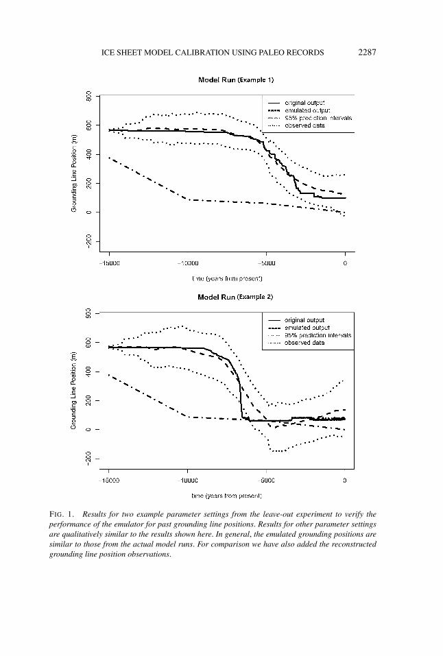
Before calibration, we verified the performance of our emulators through sep-arate leave-out experiments for each emulator η and ψ . In each experiment weleave out a group of model runs around the center of the parameter space fromthe ensemble and try to recover them using an emulator constructed based on theremaining model runs. We have left out 82 model runs for the modern binary icepatterns and 60 for the past grounding line positions since we use a smaller num-ber of model runs to emulate the grounding line position output (q = 461) thanthe modern binary pattern output (p = 625). Some examples of the comparisonresults are shown in Figures 1 (for the past grounding line positions) and 2 (for themodern binary patterns). The results show that our emulators can approximate thetrue model output reasonably well.

4.1. Simulated example. In this subsection we describe our calibration re-sults based on simulated observations to study how accurately our method recov-ers the assumed true parameter setting and its corresponding true projected icevolume change. The assumed-true parameter setting that we choose to use hereis OCFAC = 0.5, CALV = 0.5, CRH = 0.5 and TAU = 0.4 (rescaled to [0,1]),which correspond to OCFAC = 1 (nondimensional), CALV = 1 (nondimensional),CRH = 10−7 (m/year Pa2) and approximately TAU = 2.6 (k year) in the originalscale. This is one of the design points that is closest to the center of the parameterspace.

To represent the presence of model-observation discrepancy, we contaminatethe model outputs at the true parameter setting with simulated structural errors.We generate simulated errors for the past grounding line positions from a Gaus-sian process model with zero mean and the covariance defined by the squared ex-ponential function with a sill of 90 m and a range of 10,500 years. The generated

ICE SHEET MODEL CALIBRATION USING PALEO RECORDS 2287

FIG. 1. Results for two example parameter settings from the leave-out experiment to verify theperformance of the emulator for past grounding line positions. Results for other parameter settingsare qualitatively similar to the results shown here. In general, the emulated grounding positions aresimilar to those from the actual model runs. For comparison we have also added the reconstructedgrounding line position observations.

2288 CHANG, HARAN, APPLEGATE AND POLLARD

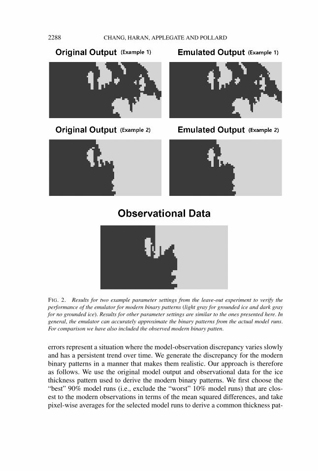
FIG. 2. Results for two example parameter settings from the leave-out experiment to verify theperformance of the emulator for modern binary patterns (light gray for grounded ice and dark grayfor no grounded ice). Results for other parameter settings are similar to the ones presented here. Ingeneral, the emulator can accurately approximate the binary patterns from the actual model runs.For comparison we have also included the observed modern binary patten.

errors represent a situation where the model-observation discrepancy varies slowlyand has a persistent trend over time. We generate the discrepancy for the modernbinary patterns in a manner that makes them realistic. Our approach is thereforeas follows. We use the original model output and observational data for the icethickness pattern used to derive the modern binary patterns. We first choose the“best” 90% model runs (i.e., exclude the “worst” 10% model runs) that are clos-est to the modern observations in terms of the mean squared differences, and takepixel-wise averages for the selected model runs to derive a common thickness pat-

ICE SHEET MODEL CALIBRATION USING PALEO RECORDS 2289

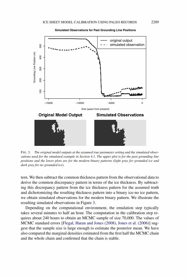
FIG. 3. The original model outputs at the assumed true parameter setting and the simulated obser-vations used for the simulated example in Section 4.1. The upper plot is for the past grounding linepositions and the lower plots are for the modern binary patterns (light gray for grounded ice anddark gray for no grounded ice).

tern. We then subtract the common thickness pattern from the observational data toderive the common discrepancy pattern in terms of the ice thickness. By subtract-ing this discrepancy pattern from the ice thickness pattern for the assumed truthand dichotomizing the resulting thickness pattern into a binary ice-no ice pattern,we obtain simulated observations for the modern binary pattern. We illustrate theresulting simulated observations in Figure 3.

Depending on the computational environment, the emulation step typicallytakes several minutes to half an hour. The computation in the calibration step re-quires about 240 hours to obtain an MCMC sample of size 70,000. The values ofMCMC standard errors [Flegal, Haran and Jones (2008), Jones et al. (2006)] sug-gest that the sample size is large enough to estimate the posterior mean. We havealso compared the marginal densities estimated from the first half the MCMC chainand the whole chain and confirmed that the chain is stable.

2290 CHANG, HARAN, APPLEGATE AND POLLARD

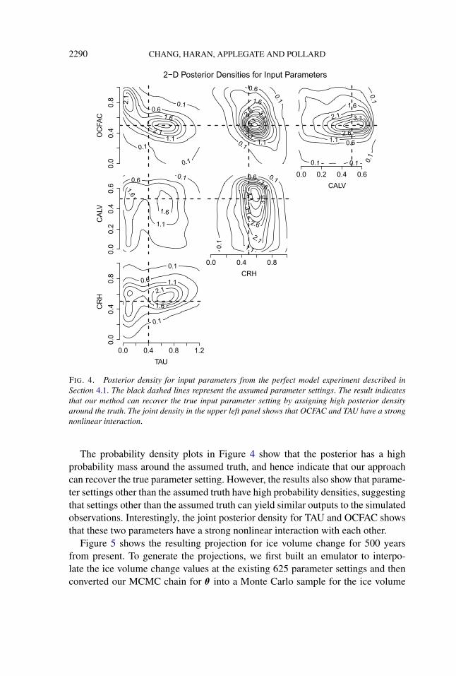
FIG. 4. Posterior density for input parameters from the perfect model experiment described inSection 4.1. The black dashed lines represent the assumed parameter settings. The result indicatesthat our method can recover the true input parameter setting by assigning high posterior densityaround the truth. The joint density in the upper left panel shows that OCFAC and TAU have a strongnonlinear interaction.

The probability density plots in Figure 4 show that the posterior has a highprobability mass around the assumed truth, and hence indicate that our approachcan recover the true parameter setting. However, the results also show that parame-ter settings other than the assumed truth have high probability densities, suggestingthat settings other than the assumed truth can yield similar outputs to the simulatedobservations. Interestingly, the joint posterior density for TAU and OCFAC showsthat these two parameters have a strong nonlinear interaction with each other.

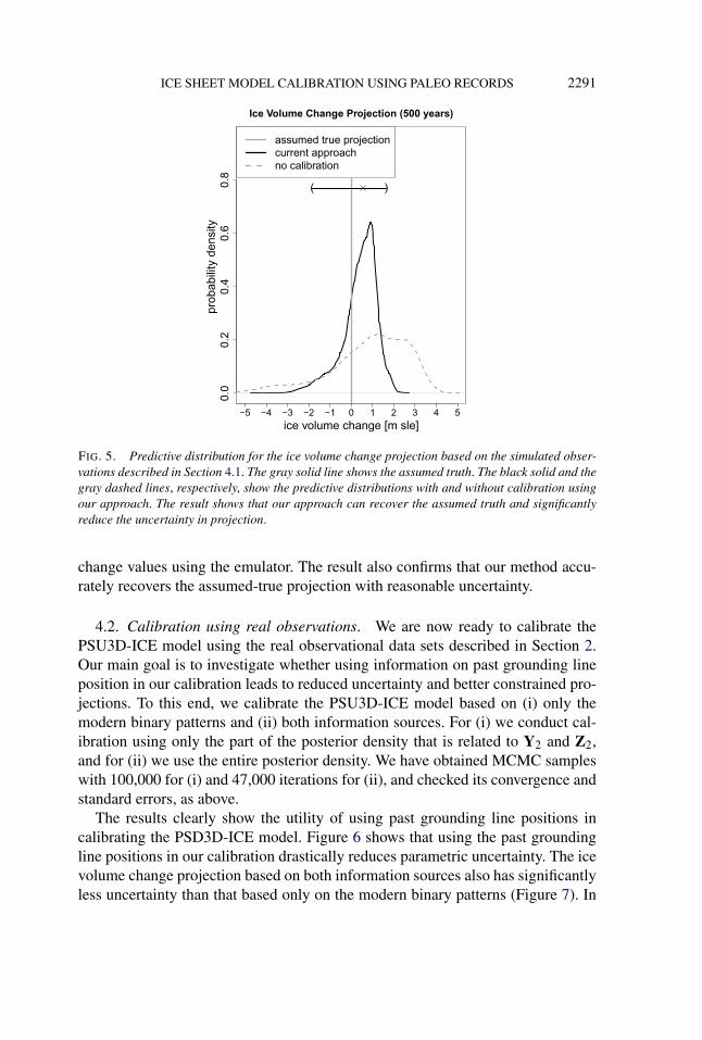
Figure 5 shows the resulting projection for ice volume change for 500 yearsfrom present. To generate the projections, we first built an emulator to interpo-late the ice volume change values at the existing 625 parameter settings and thenconverted our MCMC chain for θ into a Monte Carlo sample for the ice volume

ICE SHEET MODEL CALIBRATION USING PALEO RECORDS 2291

FIG. 5. Predictive distribution for the ice volume change projection based on the simulated obser-vations described in Section 4.1. The gray solid line shows the assumed truth. The black solid and thegray dashed lines, respectively, show the predictive distributions with and without calibration usingour approach. The result shows that our approach can recover the assumed truth and significantlyreduce the uncertainty in projection.

change values using the emulator. The result also confirms that our method accu-rately recovers the assumed-true projection with reasonable uncertainty.

4.2. Calibration using real observations. We are now ready to calibrate thePSU3D-ICE model using the real observational data sets described in Section 2.Our main goal is to investigate whether using information on past grounding lineposition in our calibration leads to reduced uncertainty and better constrained pro-jections. To this end, we calibrate the PSU3D-ICE model based on (i) only themodern binary patterns and (ii) both information sources. For (i) we conduct cal-ibration using only the part of the posterior density that is related to Y2 and Z2,and for (ii) we use the entire posterior density. We have obtained MCMC sampleswith 100,000 for (i) and 47,000 iterations for (ii), and checked its convergence andstandard errors, as above.

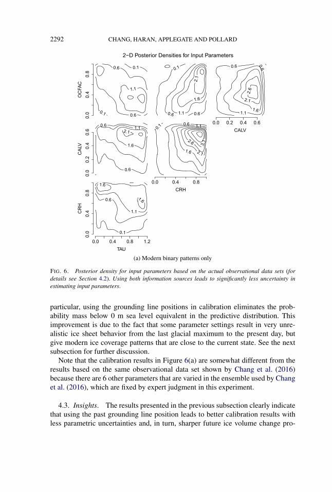
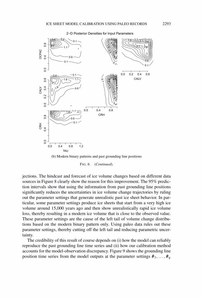
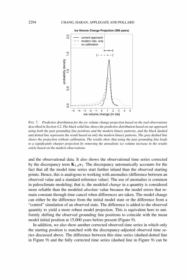
The results clearly show the utility of using past grounding line positions incalibrating the PSD3D-ICE model. Figure 6 shows that using the past groundingline positions in our calibration drastically reduces parametric uncertainty. The icevolume change projection based on both information sources also has significantlyless uncertainty than that based only on the modern binary patterns (Figure 7). In

2292 CHANG, HARAN, APPLEGATE AND POLLARD

(a) Modern binary patterns only

FIG. 6. Posterior density for input parameters based on the actual observational data sets (fordetails see Section 4.2). Using both information sources leads to significantly less uncertainty inestimating input parameters.

particular, using the grounding line positions in calibration eliminates the prob-ability mass below 0 m sea level equivalent in the predictive distribution. Thisimprovement is due to the fact that some parameter settings result in very unre-alistic ice sheet behavior from the last glacial maximum to the present day, butgive modern ice coverage patterns that are close to the current state. See the nextsubsection for further discussion.

Note that the calibration results in Figure 6(a) are somewhat different from theresults based on the same observational data set shown by Chang et al. (2016)because there are 6 other parameters that are varied in the ensemble used by Changet al. (2016), which are fixed by expert judgment in this experiment.

4.3. Insights. The results presented in the previous subsection clearly indicatethat using the past grounding line position leads to better calibration results withless parametric uncertainties and, in turn, sharper future ice volume change pro-

ICE SHEET MODEL CALIBRATION USING PALEO RECORDS 2293

(b) Modern binary patterns and past grounding line positions

FIG. 6. (Continued).

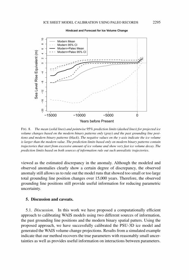
jections. The hindcast and forecast of ice volume changes based on different datasources in Figure 8 clearly show the reason for this improvement. The 95% predic-tion intervals show that using the information from past grounding line positionssignificantly reduces the uncertainties in ice volume change trajectories by rulingout the parameter settings that generate unrealistic past ice sheet behavior. In par-ticular, some parameter settings produce ice sheets that start from a very high icevolume around 15,000 years ago and then show unrealistically rapid ice volumeloss, thereby resulting in a modern ice volume that is close to the observed value.These parameter settings are the cause of the left tail of volume change distribu-tions based on the modern binary pattern only. Using paleo data rules out theseparameter settings, thereby cutting off the left tail and reducing parametric uncer-tainty.

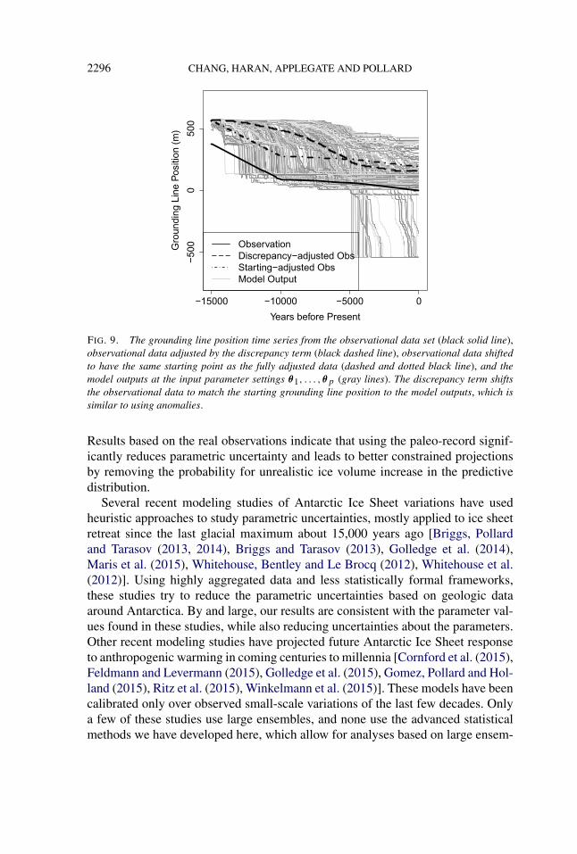
The credibility of this result of course depends on (i) how the model can reliablyreproduce the past grounding line time series and (ii) how our calibration methodaccounts for the model-observation discrepancy. Figure 9 shows the grounding lineposition time series from the model outputs at the parameter settings θ1, . . . , θq

2294 CHANG, HARAN, APPLEGATE AND POLLARD

FIG. 7. Predictive distribution for the ice volume change projection based on the real observationsdescribed in Section 4.2. The black solid line shows the predictive distribution based on our approachusing both the past grounding line positions and the modern binary patterns, and the black dashedand dotted line represents the result based on only the modern binary patterns. The gray dashed lineshows the projection without calibration. The results show that using the past grounding line leadsto a significantly sharper projection by removing the unrealistic ice volume increase in the resultssolely based on the modern observations.

and the observational data. It also shows the observational time series correctedby the discrepancy term K1,dν1. The discrepancy automatically accounts for thefact that all the model time series start further inland than the observed startingpoints. Hence, this is analogous to working with anomalies (difference between anobserved value and a standard reference value). The use of anomalies is commonin paleoclimate modeling; that is, the modeled change in a quantity is consideredmore reliable than the modeled absolute value because the model errors that re-main constant through time cancel when differences are taken. The model changecan either be the difference from the initial model state or the difference from a“control” simulation of an observed state. The difference is added to the observedquantity to yield a more robust model projection. This is equivalent here to uni-formly shifting the observed grounding line positions to coincide with the meanmodel initial position at 15,000 years before present (Figure 9).

In addition, we also show another corrected observed time series in which onlythe starting position is matched with the discrepancy-adjusted observed time se-ries discussed above. The difference between this time series (dashed-dotted linein Figure 9) and the fully corrected time series (dashed line in Figure 9) can be

ICE SHEET MODEL CALIBRATION USING PALEO RECORDS 2295

FIG. 8. The mean (solid lines) and pointwise 95% prediction limits (dashed lines) for projected icevolume changes based on the modern binary patterns only (gray) and the past grounding line posi-tions and modern binary patterns (black). The negative values on the y-axis indicate the ice volumeis larger than the modern value. The prediction limits based only on modern binary patterns containtrajectories that start from excessive amount of ice volume and show very fast ice volume decay. Theprediction limits based on both sources of information rule out such unrealistic trajectories.

viewed as the estimated discrepancy in the anomaly. Although the modeled andobserved anomalies clearly show a certain degree of discrepancy, the observedanomaly still allows us to rule out the model runs that showed too small or too largetotal grounding line position changes over 15,000 years. Therefore, the observedgrounding line positions still provide useful information for reducing parametricuncertainty.

5. Discussion and caveats.

5.1. Discussion. In this work we have proposed a computationally efficientapproach to calibrating WAIS models using two different sources of information,the past grounding line positions and the modern binary spatial patters. Using theproposed approach, we have successfully calibrated the PSU-3D ice model andgenerated the WAIS volume change projections. Results from a simulated exampleindicate that our method recovers the true parameters with reasonably small uncer-tainties as well as provides useful information on interactions between parameters.

2296 CHANG, HARAN, APPLEGATE AND POLLARD

FIG. 9. The grounding line position time series from the observational data set (black solid line),observational data adjusted by the discrepancy term (black dashed line), observational data shiftedto have the same starting point as the fully adjusted data (dashed and dotted black line), and themodel outputs at the input parameter settings θ1, . . . , θp (gray lines). The discrepancy term shiftsthe observational data to match the starting grounding line position to the model outputs, which issimilar to using anomalies.

Results based on the real observations indicate that using the paleo-record signif-icantly reduces parametric uncertainty and leads to better constrained projectionsby removing the probability for unrealistic ice volume increase in the predictivedistribution.

Several recent modeling studies of Antarctic Ice Sheet variations have usedheuristic approaches to study parametric uncertainties, mostly applied to ice sheetretreat since the last glacial maximum about 15,000 years ago [Briggs, Pollardand Tarasov (2013, 2014), Briggs and Tarasov (2013), Golledge et al. (2014),Maris et al. (2015), Whitehouse, Bentley and Le Brocq (2012), Whitehouse et al.(2012)]. Using highly aggregated data and less statistically formal frameworks,these studies try to reduce the parametric uncertainties based on geologic dataaround Antarctica. By and large, our results are consistent with the parameter val-ues found in these studies, while also reducing uncertainties about the parameters.Other recent modeling studies have projected future Antarctic Ice Sheet responseto anthropogenic warming in coming centuries to millennia [Cornford et al. (2015),Feldmann and Levermann (2015), Golledge et al. (2015), Gomez, Pollard and Hol-land (2015), Ritz et al. (2015), Winkelmann et al. (2015)]. These models have beencalibrated only over observed small-scale variations of the last few decades. Onlya few of these studies use large ensembles, and none use the advanced statisticalmethods we have developed here, which allow for analyses based on large ensem-

ICE SHEET MODEL CALIBRATION USING PALEO RECORDS 2297

bles and unaggregated data sets. Furthermore, we are able to obtain projections aswell as parameter inference in the form of genuine probability distributions, andwe take into account potential data-model discrepancies that are ignored by otherstudies. This allows us to provide uncertainties about our estimates and projec-tions.

5.2. Caveats and future directions. One caveat in our calibration model spec-ification is that we do not take into account the dependence between the pastgrounding line positions and the modern binary patterns. However, we note thatthe past grounding line positions and the modern binary patterns contain quitedifferent information since two model runs with very different trajectories of pastgrounding line position often end up with very similar modern binary patterns; thisis corroborated by an examination of cross-correlations. Developing a calibrationapproach based on the generalized principal component analysis that reduces thedimensionality of Gaussian and binary data simultaneously and computes commonprincipal component scores for both data sets is one possible future direction.

Our results are also subject to the usual caveats in ice sheet modeling. For ex-ample, we use simplified atmospheric conditions for projections, which assumethat atmospheric and oceanic temperatures linearly increase until 150 years afterpresent and stay constant thereafter. Using more detailed warming scenarios is asubject for further work. Another caveat for the present study is the use of coarse-grid global ocean model results to parameterize past basal melting under floatingice shelves. Fine-grid modeling of ocean circulation in Antarctic embayments ischallenging and a topic for further work [e.g., Hellmer et al. (2012)]. Another im-provement will be the use of finer scale models with higher-order ice dynamics,which, as discussed in the Introduction, are not quite feasible for the large spaceand time scales of this study, but should gradually become practical in the nearfuture.

APPENDIX A: COMPUTATION IN REDUCED-DIMENSIONAL SPACE

For faster computation we infer θ and other parameters in the model based onthe following dimension-reduced version of the observational data for the pastgrounding line positions:

ZR1 = (

KT1 K1

)−1KT1 Z1 =

(η(θ ,YR

1)

ν1

)+ (

KT1 K1

)−1KT1 ε1,

where K1 = (K1,y K1,d), which leads to the probability model

(8) ZR1 |ν2 ∼ N

((μη

μν1|ν2

),

(�η 00 �ν1|ν2

)+ σ 2

ε

(KT

1 K1)−1

).

The J1-dimensional vector μη and J1 × J1 matrix η are the mean and varianceof η(θ ,YR

1 ). The M-dimensional vector μν1|ν2and M × M matrix �ν1|ν2 are the

2298 CHANG, HARAN, APPLEGATE AND POLLARD

conditional mean and variance of ν1 given ν2, which can be computed as

μν1|ν2= 1

α22

Rνν2,

�ν1|ν2 = α21(IM − RνRT

ν

).

Using the likelihood function corresponding to this probability model and somestandard prior specification for θ , α2

1 and σ 2ε (see Section 4 for details), we can

infer the parameters via Markov chain Monte Carlo (MCMC). The computationalcost for likelihood evaluation reduces from 1

3n3 to 13(J1 + M)3.

APPENDIX B: DETAILED DESCRIPTION FOR THE POSTERIORDENSITY BASED ON THE MODEL SPECIFICATION IN SECTION 3.2.3

The parameters that we estimate in the equations in (5) and (6) are the in-put parameter θ (which is our main target), the variance of the i.i.d. observa-tional errors for the grounding line positions σ 2

ε , coefficients for the emulator termψ = ψ(θ ,YR

2 ), the coefficients for the discrepancy term for the modern binary pat-tern ν2, and the variances of ν1 and ν2, α2

1 and α22 . In addition to these parameters,

we also re-estimate the sill parameters for the emulator η, κ1 = [κ1,1, . . . , κ1,J1][cf. Bayarri et al. (2007), Bhat et al. (2012), Chang et al. (2014a)] to account fora possible scale mismatch between the computer model output Y1 and the ob-servational data Z1. However, we do not re-estimate the sill parameters for ψ ,κ2,1, . . . , κ2,J2 , since both Y2 and Z2 are binary responses, and hence a scalingissue is not likely to occur here; in fact, we have found that re-estimating theseparameters causes identifiability issues between the emulator term K2,yψ(θ ,YR

2 )

and the discrepancy term K2,dν2.The posterior density can be written as

π(θ ,ψ,κ1, ν2, α

21, α

22, σ

2ε ,Rν |YR

1 ,ZR1 ,YR

2 ,Z2)

∝ L(ZR

1 |YR1 , θ,κ1, α

21, σ 2

ε , ν2,Rν

)× f (κ1)f

(α2

1)f

(σ 2

ε

)f (Rν)

× L(Z2|ψ, ν2)

× f(ψ |θ ,YR

2)f

(ν2|α2

2)f

(α2

2)

× f (θ).

The likelihood function L(ZR1 |YR

1 , θ,κ1, α21, σ

2ε , ν2,Rν) is given by the proba-

bility model in (8). For f (κ1) = f (κ1,1, . . . , κ1,J1) we use independent inversegamma priors with a shape parameter of 50 and scale parameters specified in a waythat the modes of the densities coincide with the estimated values of κ1,1, . . . , κ1,J1

from the emulation stage. We assign a vague prior IG(2,3) for f (α21), f (α2

2) and

ICE SHEET MODEL CALIBRATION USING PALEO RECORDS 2299

f (σ 2ε ), and a uniform prior for f (θ) whose support is defined by the range of

design points θ1, . . . , θp . The likelihood function L(Z2|ψ, ν2) is defined as

L(Z2|ψ, ν2) ∝n∏

j=1

(exp(λj )

1 + exp(λj )

)Z2(sj )( 1

1 + exp(λj )

)1−Z2(sj )

,

where λj is the j th element of λ in (6). The conditional density f (ψ |θ ,YR2 )

is given by the Gaussian process emulator ψ(θ ,YR2 ). The conditional density

f (ν2|α22) is defined by the model ν2 ∼ N(0, α2

2IL). The prior density f (Rν) isdefined as

M∏i=1

L∏j=1

I (−1 < ρν,i,j < 1) · I (IM − RνRT

ν is positive definite),

where I (·) is the indicator function and ρν,i,j is the (i, j)th element of Rν .

Acknowledgments. We are grateful to A. Landgraf for distributing hiscode for logistic PCA freely on the Web (https://github.com/andland/SparseLogisticPCA). All views, errors and opinions are solely those of the authors.

SUPPLEMENTARY MATERIAL

Supplement to “Improving ice sheet model calibration using paleo and 2modern observations: A reduced dimensional approach” (DOI: 10.1214/16-AOAS979SUPP; .pdf). We provide additional supporting plots that show moreexample model outputs for modern binary patterns and the leading principal com-ponents used in our calibration method.

REFERENCES

APPLEGATE, P. J., KIRCHNER, N., STONE, E. J., KELLER, K. and GREVE, R. (2012). An as-sessment of key model parametric uncertainties in projections of Greenland ice sheet behavior.Cryosphere 6 589–606.

BAYARRI, M. J., BERGER, J. O., CAFEO, J., GARCIA-DONATO, G., LIU, F., PALOMO, J.,PARTHASARATHY, R. J., PAULO, R., SACKS, J. and WALSH, D. (2007). Computer model vali-dation with functional output. Ann. Statist. 35 1874–1906. MR2363956

BHAT, K. S., HARAN, M. and GOES, M. (2010). Computer model calibration with multivariatespatial output: A case study. In Frontiers of Statistical Decision Making and Bayesian Analysis(M. H. Chen, P. Müller, D. Sun, K. Ye and D. K. Dey, eds.) 168–184. Springer, New York.

BHAT, K. S., HARAN, M., OLSON, R. and KELLER, K. (2012). Inferring likelihoods and climatesystem characteristics from climate models and multiple tracers. Environmetrics 23 345–362.MR2935569

BINDSCHADLER, R. A., NOWICKI, S., ABE-OUCHI, A., ASCHWANDEN, A., CHOI, H., FAS-TOOK, J., GRANZOW, G., GREVE, R., GUTOWSKI, G., HERZFELD, U., JACKSON, C.,JOHNSON, J., KHROULEV, C., LEVERMANN, A., LIPSCOMB, W. H., MARTIN, M. A.,MORLIGHEM, M., PARIZEK, B. R., POLLARD, D., PRICE, S. F., REN, D., SAITO, F., SATO, T.,SEDDIK, H., SEROUSSI, H., TAKAHASHI, K., WALKER, R. and WANG, W. L. (2013). Ice-sheet model sensitivities to environmental forcing and their use in projecting future sea level (theSeaRISE project). J. Glaciol. 59 195–224.

2300 CHANG, HARAN, APPLEGATE AND POLLARD

BRIGGS, R., POLLARD, D. and TARASOV, L. (2013). A glacial systems model configured for largeensemble analysis of Antarctic deglaciation. Cryosphere 7 1533–1589.

BRIGGS, R. D., POLLARD, D. and TARASOV, L. (2014). A data-constrained large ensemble analysisof Antarctic evolution since the Eemian. Quat. Sci. Rev. 103 91–115.

BRIGGS, R. D. and TARASOV, L. (2013). How to evaluate model-derived deglaciation chronologies:A case study using Antarctica. Quat. Sci. Rev. 63 109–127.

BRYNJARSDÓTTIR, J. and O’HAGAN, A. (2014). Learning about physical parameters: The impor-tance of model discrepancy. Inverse Probl. 30 114007, 24. MR3274591

CHANG, W., HARAN, M., OLSON, R. and KELLER, K. (2014a). Fast dimension-reduced climatemodel calibration and the effect of data aggregation. Ann. Appl. Stat. 8 649–673. MR3262529

CHANG, W., APPLEGATE, P., HARAN, H. and KELLER, K. (2014b). Probabilistic calibration of aGreenland ice sheet model using spatially-resolved synthetic observations: Toward projections ofice mass loss with uncertainties. Geosci. Model Dev. 7 1933–1943.

CHANG, W., HARAN, M., APPLEGATE, P. and POLLARD, D. (2016). Supplement to “Improving icesheet model calibration using paleoclimate and modern data.” DOI:10.1214/16-AOAS979SUPP.

CHANG, W., HARAN, M., APPLEGATE, P. and POLLARD, D. (2016). Calibrating an ice sheet modelusing high-dimensional binary spatial data. J. Amer. Statist. Assoc. 111 57–72. MR3494638

CORNFORD, S. L., MARTIN, D. F., PAYNE, A. J., NG, E. G., LE BROCQ, A. M., GLAD-STONE, R. M., EDWARDS, T. L., SHANNON, S. R., AGOSTA, C., VAN DEN BROEKE, M. R.,HELLMER, H. H., KRINNER, G., LIGTENBERG, S. R. M., TIMMERMANN, R. andVAUGHAN, D. G. (2015). Century-scale simulations of the response of the West Antarctic IceSheet to a warming climate. Cryosphere 9 1579–1600.

FAVIER, L., DURAND, G., CORNFORD, S. L., GUDMUNDSSON, G. H., GAGLIARDINI, O.,GILLET-CHAULET, F., ZWINGER, T., PAYNE, A. J. and LE BROCQ, A. M. (2014). Retreat ofPine Island Glacier controlled by marine ice-sheet instability. Nature Climate Change 4 171–121.

FELDMANN, J. and LEVERMANN, A. (2015). Collapse of the West Antarctic Ice Sheet after localdestabilization of the Amundsen Basin. Proc. Natl. Acad. Sci. USA 112 14191–14196.

FLEGAL, J. M., HARAN, M. and JONES, G. L. (2008). Markov chain Monte Carlo: Can we trustthe third significant figure? Statist. Sci. 23 250–260. MR2516823

FRETWELL, P., PRITCHARD, H. D., VAUGHAN, D. G., BAMBER, J. L., BARRAND, N. E.,BELL, R., BIANCHI, C., BINGHAM, R. G., BLANKENSHIP, D. D., CASASSA, G., CATA-NIA, G., CALLENS, D., CONWAY, H., COOK, A. J., CORR, H. F. J., DAMASKE, D., DAMM, V.,FERRACCIOLI, F., FORSBERG, R., FUJITA, S., GIM, Y., GOGINENI, P., GRIGGS, J. A., HIND-MARSH, R. C. A., HOLMLUND, P., HOLT, J. W., JACOBEL, R. W., JENKINS, A., JOKAT, W.,JORDAN, T., KING, E. C., KOHLER, J., KRABILL, W., RIGER-KUSK, M., LANGLEY, K. A.,LEITCHENKOV, G., LEUSCHEN, C., LUYENDYK, B. P., MATSUOKA, K., MOUGINOT, J.,NITSCHE, F. O., NOGI, Y., NOST, O. A., POPOV, S. V., RIGNOT, E., RIPPIN, D. M.,RIVERA, A., ROBERTS, J., ROSS, N., SIEGERT, M. J., SMITH, A. M., STEINHAGE, D.,STUDINGER, M., SUN, B., TINTO, B. K., WELCH, B. C., WILSON, D., YOUNG, D. A., XI-ANGBIN, C. and ZIRIZZOTTI, A. (2013). Bedmap2: Improved ice bed, surface and thicknessdatasets for Antarctica. Cryosphere 7 375–393.

GLADSTONE, R. M., LEE, V., ROUGIER, J., PAYNE, A. J., HELLMER, H., LE BROCQ, A., SHEP-HERD, A., EDWARDS, T. L., GREGORY, J. and CORNFORD, S. L. (2012). Calibrated predictionof Pine Island Glacier retreat during the 21st and 22nd centuries with a coupled flowline model.Earth Planet. Sci. Lett. 333 191–199.

GOLLEDGE, N. R., MENVIEL, L., CARTER, L., FOGWILL, C. J., ENGLAND, M. H., CORTESE, G.and LEVY, R. H. (2014). Antarctic contribution to meltwater pulse 1A from reduced SouthernOcean overturning. Nature Comm. 5.

GOLLEDGE, N. R., KOWALEWSKI, D. E., NAISH, T. R., LEVY, R. H., FOGWILL, C. J. and GAS-SON, E. G. W. (2015). The multi-millennial Antarctic commitment to future sea-level rise. Nature526 421–425.

ICE SHEET MODEL CALIBRATION USING PALEO RECORDS 2301

GOMEZ, N., POLLARD, D. and HOLLAND, D. (2015). Sea-level feedback lowers projections offuture Antarctic ice-sheet mass loss. Nature Comm. 6.

HASTIE, T., TIBSHIRANI, R. and FRIEDMAN, J. (2009). The Elements of Statistical Learning: DataMining, Inference, and Prediction, 2nd ed. Springer, New York. MR2722294

HELLMER, H. H., KAUKER, F., TIMMERMANN, R., DETERMANN, J. and RAE, J. (2012). Twenty-first-century warming of a large Antarctic ice-shelf cavity by a redirected coastal current. Nature485 225–228.

HIGDON, D., GATTIKER, J., WILLIAMS, B. and RIGHTLEY, M. (2008). Computer model calibra-tion using high-dimensional output. J. Amer. Statist. Assoc. 103 570–583. MR2523994

JONES, G. L., HARAN, M., CAFFO, B. S. and NEATH, R. (2006). Fixed-width output analysis forMarkov chain Monte Carlo. J. Amer. Statist. Assoc. 101 1537–1547. MR2279478

JOUGHIN, I., SMITH, B. E. and MEDLEY, B. (2014). Marine ice sheet collapse potentially underway for the Thwaites Glacier Basin, West Antarctica. Science 344 735–738.

KENNEDY, M. C. and O’HAGAN, A. (2001). Bayesian calibration of computer models. J. R. Stat.Soc. Ser. B. Stat. Methodol. 63 425–464. MR1858398

KIRSHNER, A. E., ANDERSON, J. B., JAKOBSSON, M., O’REGAN, M., MAJEWSKI, W. andNITSCHE, F. O. (2012). Post-LGM deglaciation in Pine Island Bay, West Antarctica. Quat. Sci.Rev. 38 11–26.

LARTER, R. D., ANDERSON, J. B., GRAHAM, A. G., GOHL, K., HILLENBRAND, C.-D., JAKOBS-SON, M., JOHNSON, J. S., KUHN, G., NITSCHE, F. O. and SMITH, J. A. (2014). Reconstructionof changes in the Amundsen Sea and Bellingshausen sea sector of the West Antarctic Ice Sheetsince the last glacial maximum. Quat. Sci. Rev. 100 55–86.

LEMPERT, R., SRIVER, R. L. and KELLER, K. (2012). Characterizing uncertain sea level riseprojections to support investment decisions. California Energy Commission. Publication Number:CEC-500-2012-056.

LIU, Z., OTTO-BLIESNER, B. L., HE, F., BRADY, E. C., TOMAS, R., CLARK, P. U., CARL-SON, A. E., LYNCH-STIEGLITZ, J., CURRY, W., BROOK, E., ERICKSON, D., JACOB, R.,KUTZBACH, J. and CHENG, J. (2009). Transient simulation of last deglaciation with a new mech-anism for Bølling–Allerød warming. Science 325 310–314.

MARIS, M. N. A., VAN WESSEM, J. M., VAN DE BERG, W. J., DE BOER, B. and OERLE-MANS, J. (2015). A model study of the effect of climate and sea-level change on the evolution ofthe Antarctic Ice Sheet from the Last Glacial Maximum to 2100. Clim. Dynam. 45 837–851.

MCNEALL, D. J., CHALLENOR, P. G., GATTIKER, J. R. and STONE, E. J. (2013). The potential ofan observational data set for calibration of a computationally expensive computer model. Geosci.Model Dev. 6 1715–1728.

POLLARD, D. and DECONTO, R. M. (2009). Modelling West Antarctic Ice Sheet growth and col-lapse through the past five million years. Nature 458 329–332.

POLLARD, D. and DECONTO, R. M. (2012a). A simple inverse method for the distribution of basalsliding coefficients under ice sheets, applied to Antarctica. Cryosphere 6 1405–1444.

POLLARD, D. and DECONTO, R. M. (2012b). Description of a hybrid ice sheet-shelf model, andapplication to Antarctica. Geosci. Model Dev. 5 1273–1295.

PRITCHARD, H. D., LIGTENBERG, S. R. M., FRICKER, H. A., VAUGHAN, D. G., VAN DEN

BROEKE, M. R. and PADMAN, L. (2012). Antarctic ice-sheet loss driven by basal melting of iceshelves. Nature 484 502–505.

RAISED CONSORTIUM (2014). A community-based geological reconstruction of Antarctic IceSheet deglaciation since the Last Glacial Maximum. Quat. Sci. Rev. 100 1–9.

RITZ, C., EDWARDS, T. L., DURAND, G., PAYNE, A. J., PEYAUD, V. and HINDMARSH, R. C.(2015). Potential sea-level rise from Antarctic ice-sheet instability constrained by observations.Nature 528 115–118.

SACKS, J., WELCH, W. J., MITCHELL, T. J. and WYNN, H. P. (1989). Design and analysis ofcomputer experiments. Statist. Sci. 4 409–435. MR1041765

2302 CHANG, HARAN, APPLEGATE AND POLLARD

STONE, E. J., LUNT, D. J., RUTT, I. C. and HANNA, E. (2010). Investigating the sensitivity of nu-merical model simulations of the modern state of the Greenland ice-sheet and its future responseto climate change. Cryosphere 4 397–417.

WHITEHOUSE, P. L., BENTLEY, M. J. and LE BROCQ, A. M. (2012). A deglacial model for Antarc-tica: Geological constraints and glaciological modeling as a basis for a new model of Antarcticglacial isostatic adjustment. Quat. Sci. Rev. 32 1–24.

WHITEHOUSE, P. L., BENTLEY, M. J., MILNE, G. A., KING, M. A. and THOMAS, I. D. (2012).A new glacial isostatic model for Antarctica: Calibrated and tested using observations of relativesea-level change and present-day uplifts. Geophysical Journal International 190 1464–1482.

WINKELMANN, R., LEVERMANN, A., RIDGWELL, A. and CALDEIRA, K. (2015). Combustion ofavailable fossil fuel resources sufficient to eliminate the Antarctic Ice Sheet. Sci. Adv. 1 e1500589.

W. CHANG

DEPARTMENT OF MATHEMATICAL SCIENCES

UNIVERSITY OF CINCINNATI

CINCINNATI, OHIO 45221USAE-MAIL: won.chang@uc.edu

M. HARAN

DEPARTMENT OF STATISTICS

PENNSYLVANIA STATE UNIVERSITY

UNIVERSITY PARK, PENNSYLVANIA 16802USAE-MAIL: mharan@stat.psu.edu

P. APPLEGATE

D. POLLARD

EARTH AND ENVIRONMENTAL SYSTEMS INSTITUTE

PENNSYLVANIA STATE UNIVERSITY

UNIVERSITY PARK, PENNSYLVANIA 16802USAE-MAIL: patrick.applegate@psu.edu

pollard@essc.psu.edu