IMPROVING HEMODIALYSIS TREATMENT: MODELING, EXPERIMENTAL ...
213
IMPROVING HEMODIALYSIS TREATMENT: MODELING, EXPERIMENTAL DESIGN, AND CLINICAL STUDIES VAIBHAV MAHESHWARI NATIONAL UNIVERSITY OF SINGAPORE 2013
Transcript of IMPROVING HEMODIALYSIS TREATMENT: MODELING, EXPERIMENTAL ...

IMPROVING HEMODIALYSIS TREATMENT:
MODELING, EXPERIMENTAL DESIGN, AND
CLINICAL STUDIES
VAIBHAV MAHESHWARI
NATIONAL UNIVERSITY OF SINGAPORE
2013

IMPROVING HEMODIALYSIS TREATMENT: MODELING, EXPERIMENTAL DESIGN, AND CLINICAL STUDIES
VAIBHAV MAHESHWARI
2013

IMPROVING HEMODIALYSIS TREATMENT:
MODELING, EXPERIMENTAL DESIGN, AND
CLINICAL STUDIES
VAIBHAV MAHESHWARI
(B.Tech., NIT Durgapur, India)
A THESIS SUBMITTED
FOR THE DEGREE OF DOCTOR OF PHILOSOPHY
DEPARTMENT OF CHEMICAL AND BIOMOLECULAR
ENGINEERING
NATIONAL UNIVERSITY OF SINGAPORE
2013


DECLARATION
I hereby declare that the thesis is my original work and it has been written
by me in its entirety. I have duly acknowledged all the sources of
information which have been used in the thesis.
This thesis has not been submitted for any degree in any university
previously.
Vaibhav Maheshwari
29 July 2013


To my teachers


Acknowledgements
vii
Acknowledgements
I used to believe that PhD is a solo journey. You have to define your research problem;
you have to articulate your thoughts; and you have to communicate it with scientific
community. Now when I have completed my PhD research work and introspect into last
few years, I can firmly say that PhD is not a solo journey. Without help of many people, I
could not have completed this. Here, I take the opportunity to say THANK YOU ALL.
First and foremost, I sincerely thank my supervisors Prof Laksh and Prof Rangaiah for
their guidance throughout this memorable journey. I will remain eternally grateful to both
of them for giving me ample freedom to pursue this research. Nevertheless, I sought their
guidance time and again. Prof Laksh enlightened me about teaching & education, writing
skills, and many facets of both personal and professional life. At the same time, I learnt to
be systematic, organized, and transparent in all activities from Prof Rangaiah. I also thank
Dr. Titus Lau for his support and guidance in clinical research.
I extend my heartfelt gratitude to my lab-mates and friends with whom I have shared my
frustration and joy, success and failures, highs and lows of PhD. I thank Naviyn with
whom I spent perhaps the maximum time in this journey. If I want to emulate the
humbleness of anyone then it would be Naviyn. I thank Shruti who has been very helpful.
She is one of those many people who helped me whenever I asked for. Her jokes always
uplifted the mood in the E5-B-02 (my sitting place). I will remain indebted to many NUS
friends: Manoj, Krishna, Shivom, Karthik Raja, KMG, Ashwini, Sumit, Vamsi, Wendou,
Bhargava, Susarla Naresh, Shailesh, Deepti & Anupam, who have been part of this
journey. They not only made this journey enjoyable but also memorable. Without friends,
this journey would only be a dream. My seniors Lakshmi Kiran and Loganathan guided
me in my early days of research and also helped me improving my presentation skills.

Acknowledgements
viii
Technical help from Sridharan Srinath immensely helped me at important junctures of my
research.
I thank NUS for financial support and NKF for providing the research grant to conduct
clinical research. I also thank research collaborators for their help in clinical research –
NUH dialysis center nurses (Aafiah, Eve, Farrah, Frances, George, Karen, Rajani, Sister
Soriani), Yijun Loy and Serene Lim (physiotherapists), Dr. Ling Lieng Hsi. I thank all the
patients who have been part of clinical study. I thank Mr. Boey and Samantha for lab
related issues, Steffen for resolving finance queries in NKF grants, Doris and Vanessa for
providing administrative support. I thank NUS library which has played an important role
in providing the required reference materials.
Then, there are persons whom I have never met personally but who have been of great
help – the first person is Dr. Richard Ward (University of Louisville) who provided the
confidential patient data which eventually directed my research, and second is Joanna
(from NKF) who unfailingly resolved my queries and acceded to all grant related queries.
I find myself very lucky to have a group of friends from Self Realization Fellowship
whom I have been meeting on Sundays. I thank them for many things which cannot be
expressed in words. In the later part of this PhD journey when my research took upswing,
I married to Anchal. She is one of those who suffered the most because of this research,
and I thank her for understanding heart. This work is the result of many prayers and well
wishes of my parents who are always worried about me. I thank my brother who has
always been an inspiration for me. Last but not the least, I thank the reader for taking time
to read this thesis.
I thank God for his unconditional love and everything.

Table of Contents
ix
SUMMARY .................................................................................................................... xiii
LIST OF TABLES ........................................................................................................... xv
LIST OF FIGURES ....................................................................................................... xvii
ABBREVIATIONS & NOTATIONS ............................................................................ xxi
1. Introduction .................................................................................................................. 1
1.1 Engineering and Medicine .................................................................................... 1
1.2 Kidneys and Kidney Failure .................................................................................. 2
1.3 Dialysis .................................................................................................................. 3
1.3.1 Peritoneal dialysis .......................................................................................... 3
1.3.2 Hemodialysis.................................................................................................. 4
1.4 Statistics ................................................................................................................ 6
1.5 Motivation and Objectives .................................................................................... 9
1.6 Thesis Organization............................................................................................. 11
Part 1 Toxin Kinetic Modeling and Clinical Study....................................................... 13
2. Literature Review: Toxin Kinetic Modeling .............................................................. 15
2.1 Toxins .................................................................................................................. 15
2.2 Uremic Toxicity and Marker Toxin(s) ................................................................ 17
2.3 Toxin Kinetic Modeling ...................................................................................... 20
2.3.1 Single-pool Model ....................................................................................... 21
2.3.2 Two-pool Model .......................................................................................... 24

Table of Contents
x
2.3.3 Multi-compartment Model ........................................................................... 27
2.3.4 Regional Blood Flow Model ........................................................................ 29
2.4 Kinetics of other toxins ....................................................................................... 31
2.4.1 Phosphate Kinetics ....................................................................................... 32
2.4.2 Sodium Kinetics and Profiling ..................................................................... 33
2.4.3 Kinetics of Guanidino Compounds .............................................................. 35
2.5 Summary ............................................................................................................. 37
3. Diffusion-adjusted Regional Blood Flow Model for β2-Microglobulin .................... 39
3.1 β2-microglobulin and Kinetic Studies ................................................................. 40
3.2 Model Description ............................................................................................... 42
3.3 Model Parameter Reduction and Estimation ....................................................... 47
3.4 Interpretation of Parameter Estimates ................................................................. 53
3.5 Model Applications ............................................................................................. 58
3.5.1 Estimation of Removed Toxin Mass............................................................ 58
3.5.2 Simulating Effect of Exercise ...................................................................... 59
3.6 Summary ............................................................................................................. 64
4. Clinical Study to Compare Toxin Removal in Hemodialysis, Hemodiafiltration, and
Hemodialysis with Exercise ............................................................................................... 65
4.1 Hemodiafiltration ................................................................................................ 66
4.1.1 Clinical Evidences for HDF ......................................................................... 68
4.2 Exercise during Dialysis...................................................................................... 71

Table of Contents
xi
4.2.1 Exercise and Temperature ............................................................................ 72
4.3 Clinical Trial Design ........................................................................................... 73
4.3.1 Study Design and Ethics Approval .............................................................. 74
4.3.2 Patient Recruitment and Inclusion-Exclusion Criteria ................................ 75
4.3.3 Study Interventions ...................................................................................... 77
4.3.4 Data collection ............................................................................................. 78
4.4 Patient and Dialysis Information ......................................................................... 80
4.5 Results from the Clinical Study .......................................................................... 83
4.6 Discussion ........................................................................................................... 87
4.7 Summary ............................................................................................................. 92
Part 2 Model-based Design of Experiments .................................................................. 95
5. Multi-Objective Framework for Model-based Design of Experiment Techniques ... 97
5.1 Mathematical Models and Experiment ............................................................... 98
5.2 Mathematics of MBDOE .................................................................................. 102
5.3 Parameter correlation ........................................................................................ 105
5.4 Multi-Objective Optimization based DOE framework ..................................... 108
5.5 Solution Approach (Genetic algorithm) ............................................................ 110
5.6 Case Studies ...................................................................................................... 111
5.6.1 Modified Bergman minimal model for Type 1 diabetes subjects .............. 114
5.6.2 Baker’s Yeast Fermentation Reactor Model .............................................. 127
5.7 Discussion ......................................................................................................... 135
Table of Contents
xii
5.8 Summary ........................................................................................................... 137
6. Optimal Sampling Protocol for Toxin Kinetic Modeling ........................................ 139
6.1 Sampling protocols in TKM .............................................................................. 139
6.2 Materials and Methods ...................................................................................... 142
6.3 Results ............................................................................................................... 146
6.4 Discussion and Sampling Recommendation ..................................................... 151
6.5 Summary ........................................................................................................... 155
7. Conclusions and Recommendations for Future Works ........................................... 157
7.1 Contributions ..................................................................................................... 158
7.1.1 Toxin Kinetic Modeling and Clinical Study .............................................. 158
7.1.2 Model-based Design of Experiments ......................................................... 162
7.2 Recommendations for Future Works ................................................................ 164
7.2.1 One TKM for All Marker Toxins .............................................................. 164
7.2.2 Clinical Study: HDF vs. HD-Ex ................................................................ 165
7.2.3 Clinical Study: Cool vs. Warm Dialysate .................................................. 166
7.2.4 Model Predictive Controller and Dialysate Temperature .......................... 168
7.2.5 Exploring Synergies between Exercise Regimen and Dialysate Temperature
168
7.2.6 MOO based DOE for Larger Systems ....................................................... 169
REFERENCES ............................................................................................................... 171

Summary
xiii
SUMMARY
Hemodialysis (HD) is a life-saving treatment option for end stage kidney disease patients.
It removes excess fluid and toxins which are normally removed by healthy kidneys.
During HD, blood is passed through hollow fiber membranes, which remove accumulated
toxins and fluid via diffusion and convection. This makes HD a perfect example of
synergy between chemical engineering principles and medical care. Although HD
sustains patients’ lives, poor patients’ outcome is a major concern. Hence, the broad focus
of this research work is to improve HD care such that it will result in better patient
outcome. One potential way to achieve this is to enhance the toxin removal, the mainstay
of HD since its inception in 1950’s. One effective way to accomplish this is via process
systems engineering (PSE) principles, especially mathematical modeling.
In HD, compartmental toxin kinetic modeling continues to play an important role in
understanding the toxin removal behavior. The present work proposes a comprehensive
kinetic model for middle-sized marker toxin (β2-microglobulin) in HD patients. One of
the major advantages of mathematical models is that, they are not restricted to explain the
underlying phenomena only, but also can be extrapolated to simulate other relevant
scenarios. Guided by this, the proposed model is expanded to explain the enhanced toxin
removal due to exercise during dialysis. Simulation results suggest that the increased
toxin removal can only be explained by a decrease in inter-compartmental resistance, the
major barrier for toxin removal. In order to verify the simulation results, a pilot scale
clinical study was conducted in the National University Hospital, Singapore. Results
indicate that exercise can lead to improved toxin removal. It is also found that the
exercise during dialysis increases the body core temperature and cardiac output resulting
in decreased compartmental resistance i.e. enhanced toxin removal. This is the first

Summary
xiv
clinical study which thoroughly investigated the exercise induced physiological changes
in HD care.
However, the clinical experiment did not quantify the decrease in inter-compartmental
resistance, which can provide better understanding of exercise induced physiological
changes and pave way for personalized prescription of intra-dialytic exercise. The inter-
compartmental resistance cannot be measured, but it can be inferred from one of the
parameters in the proposed toxin kinetic model. To estimate the model parameters, good
data should be collected. In this context, model based design of experiments (MBDoE)
techniques would be effective. However, the existing MBDoE techniques increase the
correlation among parameters, which may lead to inaccurate estimates. Therefore, they
are improved by proposing a multi-objective framework. The proposed framework is first
tested for example case studies and then for the developed toxin kinetic model. This is the
first study to investigate the optimal sampling for improving the HD model.
Overall, the thesis combines the in silico approach (of model development and
improvement via better estimation of model parameters) with the in vivo approach (of
clinical study to test the model generated hypothesis in HD care), and provides useful
results and improved techniques for improving the HD care.

List of Tables
xv
LIST OF TABLES
Table 3.1: Constant model parameters for all patients ...................................................... 51
Table 3.2: Estimated model parameters for β2-microglobulin kinetics ............................. 52
Table 3.3: Estimates of removed toxin mass (mean±s.e.m.) ............................................. 59
Table 3.4: Simulating effect of intra-dialytic exercise – Decrease in rebound % (a) for 100% increase in cardiac output (CO) and (b) for 15% increase in inter-compartmental mass transfer coefficient (Kip) ............................................................................................ 63
Table 4.1: Patient demographics at the time of consent .................................................... 81
Table 4.2: Percentage rebound for each uremic toxin in different dialysis protocols ....... 83
Table 5.1: Design variables, their bounds, and initial guess for the proposed clinical test for Type 1 diabetes subjects ............................................................................................. 117
Table 5.2: Transformation of constraints into bounds ..................................................... 119
Table 5.3: Parameter estimates and statistics for D-optimal and DMOO design ............ 122
Table 5.4: Parameter estimates and statistics for A-optimal and AMOO design ............ 124
Table 5.5: Parameter estimates and statistics for E-optimal and EMOO design ............. 125
Table 5.6: Percentage normalized Euclidean distance for alphabetical and MOO based designs for Type 1 diabetes model ................................................................................... 126
Table 5.7: Design variables, their bounds, and initial guess values for Baker's yeast fermentation reactor system ............................................................................................. 128
Table 5.8: Parameter estimates and statistics for D-optimal design and DMOO design . 131
Table 5.9: Parameter estimates and statistics for A-optimal design and AMOO design . 132
Table 5.10: Parameter estimates and statistics for E-optimal design and EMOO design 134
Table 5.11: Percentage normalized Euclidean distance for alphabetical and MOO based designs for Baker’s yeast fermentation reactor model ..................................................... 135
Table 6.1: Existing sampling protocols for various uremic toxins .................................. 141
Table 6.2: Model parameters with their known true values and initial guesses used for model-based design of experiment techniques ................................................................ 144

List of Tables
xvi
Table 6.3: Two factors – Experiment duration and number of decision variables, each at 4 levels ................................................................................................................................ 145
Table 6.4: Decision variables (d.v.) or optimal sampling instances in different experiment duration (during dialysis + post-dialysis). Sampling instances during dialysis (normal text) and post-dialysis (bold text), respectively. .............................................................. 149
Table 6.5: Point estimates (θ), t-value, and Percentage normalized Euclidean distance (δ) from true parameter for each scenario ............................................................................. 150

List of Figures
xvii
LIST OF FIGURES
Figure 1.1 Schematics of (A) peritoneal dialysis[6] and (B) hemodialysis [7] ................... 5
Figure 1.2: Block representation of Hemodialysis, Hemofiltration, and Hemodiafiltration 6
Figure 1.3: Adjusted (for race and gender) all-cause mortality in US population [11]. ...... 7
Figure 1.4: Yearly total Medicare expenditure in US by modality [11]. ............................. 9
Figure 2.1: (A) Patient (single-pool model) attached to hemodialyzer; (B) Constant volume single-pool model; and (C) Variable volume single-pool model. Vd and Cs are urea distribution volume and urea concentration in body, respectively. G is urea generation rate; KD is dialyzer urea clearance; Kr is residual renal clearance; α is fluid intake; and Quf is ultrafiltration rate. .................................................................................. 22
Figure 2.2: Two-pool model representation of physiology. Intracellular fluid volume is greater than extracellular fluid. Toxin generation is assumed to occur in intracellular compartment. ..................................................................................................................... 25
Figure 2.3: Urea kinetics modeling by single- and two-pool models. Sharp post-dialytic increase of urea concentration disproves the single-pool hypothesis for UKM ................ 27
Figure 2.4: Multi-compartmental representation of physiology. C and V denote concentration and toxin distribution volume. The suffix ‘i’ denotes intracellular compartment, ‘ei’ denote interstitial-extracellular and ‘ep’ is plasma-extracellular compartment. ..................................................................................................................... 28
Figure 2.5: Blood flow/tissue water volume and water content of different organs under baseline condition [48] ....................................................................................................... 30
Figure 2.6: Regional blood flow representation of physiology. The flow line thickness is approximately proportional to the amount of cardiac output received. QH and QL represent the amount of blood flow received by HFR and LFR, respectively; QB is the blood flow to dialyzer; Quf is ultrafiltration rate; CO is cardiac output; kH and kL are fluid fraction of HFR and LFR, respectively. .............................................................................................. 31
Figure 2.7: Phosphate kinetics model comprising four pools [56]. ................................... 33
Figure 2.8: Dialysate sodium profile to control the serum sodium concentration ............. 35
Figure 3.1: Compartmental representation of physiology. Toxins are distributed in intracellular (IC) and extracellular compartments (EC). Urea is distributed in both IC and EC, and β2M is distributed in EC. The hollow arrows between IC and interstitium denote fluid movement, while solid arrows between interstitium and plasma represent the fluid as well as β2M movement. ..................................................................................................... 40
List of Figures
xviii
Figure 3.2: Diffusion-adjusted regional blood flow model (parallel-cum-series representation of physiology) for explaining β2M kinetics. Toxin transfer is due to diffusion across capillary endothelium, and blood/plasma circulation causes convective transport. Qh/Qhp, Ql/Qlp, and Qb/Qbp are blood/plasma flows to HFR, LFR, and dialyzer, respectively. Qcr and Qar are cardiopulmonary and access recirculation, respectively. Shaded compartments represent contact with blood (A – arterial node and V – venous node). Here, IC is not presented because β2M distribution is restricted to EC alone. ....... 43
Figure 3.3: Plasma β2M concentrations during 240 min dialysis treatment and for 4 hours following the treatment. Data is presented as mean± standard error of mean (s.e.m.) [74].
............................................................................................................................................ 47
Figure 3.4: Arterial plasma concentration profile (model fit) and measured concentration of β2-microglobulin for Patient 1 (top) and Patient 10 (bottom) ....................................... 56
Figure 3.5: β2-microglobulin concentration profile in different body compartments for Patient 1 (top) and Patient 10 (bottom). ............................................................................. 57
Figure 3.6: Simulation of effect of intra-dialytic exercise for Patient 1 (top) and Patient 10 (bottom) – Decrease in post-dialysis rebound due to 100% increase in cardiac output. ... 61
Figure 4.1: Blood and dialysate flow along dialyzer length. Horizontal arrows represent transfer of accumulated toxins and excess fluid from blood to dialysate stream .............. 67
Figure 4.2: Pre- and post-dilution modes of hemodiafiltration. The given blood and dialysate flow rate are usual numbers practiced in routine dialysis settings. The replacement fluid rate is assumed to be 80 mL/min. ......................................................... 68
Figure 4.3 Blood temperature snapshot during HD session for two sample patients. In panel A, the kink in dialysate and venous temperatures is due to the measurement of access recirculation. ........................................................................................................... 80
Figure 4.4: Schematic flow-chart of clinical trial .............................................................. 82
Figure 4.5: Arterial (red - -) and Venous (blue - -) blood temperature during HD-Ex session ................................................................................................................................ 85
Figure 4.6: Patients' cardiac output and peripheral vascular resistance index during the first bout of exercise. In bottom panel, cardiac output and resistance index are presented as mean ± standard deviation. ............................................................................................ 86
Figure 5.1: Schematic of model development following the principles of model-based design of experiments techniques .................................................................................... 100
Figure 5.2: Geometrical interpretation of the D-, A-, and E-optimal design for two parameters ........................................................................................................................ 105

List of Figures
xix
Figure 5.3: Schematic representation of trade-off between information measure and correlation measure. Between the two extremes of alphabetical (D-, A-, E-) design criterion and Pritchard and Bacon criterion, experimenter has freedom to select appropriate optimal experiment design from the Pareto-optimal front. Star is one chosen design for illustration. ...................................................................................................... 112
Figure 5.4: Schematic of the design procedure followed in the case studies .................. 113
Figure 5.5: Transformation of exact time-instants into delta-time instants ..................... 118
Figure 5.6: Pareto-optimal front for DMOO design ........................................................ 121
Figure 5.7: Time profiles of basal insulin infusion and blood glucose sampling instances (●) for D-optimal and DMOO design vectors and resulting glucose concentration profiles
.......................................................................................................................................... 122
Figure 5.8: Pareto-optimal front for AMOO design ........................................................ 123
Figure 5.9: Time profiles of basal insulin infusion and blood glucose sampling instances (●) for A-optimal and AMOO design vectors and resulting glucose concentration profiles
.......................................................................................................................................... 123
Figure 5.10: Pareto-optimal front for EMOO design ....................................................... 124
Figure 5.11: Time profiles of basal insulin infusion and blood glucose sampling instances (●) for E-optimal and EMOO design vectors and resulting glucose concentration profiles
.......................................................................................................................................... 125
Figure 5.12: Pareto-optimal front for DMOO design ...................................................... 130
Figure 5.13: Time-profile of manipulated vairables ( 1u and 2u ) and sampling instances (●) for D-optimal and DMOO design .................................................................................... 130
Figure 5.14: Pareto-optimal front for AMOO design ...................................................... 131
Figure 5.15: Time-profile of manipulated vairables ( 1u and 2u ) and sampling instances (●) for A-optimal and AMOO design. ................................................................................... 132
Figure 5.16: Pareto-optimal front for EMOO design ....................................................... 133
Figure 5.17: Time-profile of manipulated vairables ( 1u and 2u ) and sampling instances (●) for E-optimal and EMOO design. .................................................................................... 133
Figure 6.1: Pareto-optimal front for 240 min experiment duration and 8 decision variables .......................................................................................................................................... 146

List of Figures
xx
Figure 6.2: Pareto-optimal front for 300 min experiment duration and 8 decision variables .......................................................................................................................................... 147
Figure 6.3: Pareto-optimal front for 360 min experiment duration and 8 decision variables .......................................................................................................................................... 147
Figure 6.4: Pareto-optimal front for 480 min experiment duration and 8 decision variables .......................................................................................................................................... 148

Abbreviations
xxi
ABBREVIATIONS & NOTATIONS
6 MWT 6-min walk test
AC Anti-correlation
ADMA Asymmetric dimethylarginine
AGE Advanced glycation end-product
ALE Advanced lipoxidation end-product
AMOO MOO based A-optimal design
β2M β2-microglobulin
BTM Blood Temperature Monitor
BUN Blood Urea Nitrogen
C Toxin concentration
C0 Pre-dialysis serum urea concentration
Cart/ven Arterial/Venous concentration
Cend End-dialysis serum urea concentration
CO Cardiac Output
CHD Conventional Hemodialysis
CHO Carbohydrates
CKD Chronic Kidney Disease
COPD Chronic Obstructive Pulmonary Disease
CRF Chronic Renal Failure

Abbreviations
xxii
Cs Solute Concentration
DAE Differential-Algebraic Equations
DA-RBF Diffusion-adjusted Regional Blood Flow
DBP Diastolic Blood Pressure
DMOO MOO based D-optimal design
DOE Design of Experiments
e Extracellular fluid volume fraction
EC Extracellular Compartment
EMOO MOO based E-optimal design
ESRD End Stage Renal Disease
FIM Fisher Information Matrix
fh/l Blood flow fraction to HFR/LFR
fP Plasma fraction in EC
FMC Fresenius Medical Care
G Toxin Generation Rate (Urea, Creatinine, β2M …)
GA Genetic Algorithm
GC Guanidino Compounds
GCP Good Clinical Practices
HCT Hematocrit
HD Hemodialysis

Abbreviations
xxiii
HDF Hemodiafiltration
HD-Ex Exercise during HD
HF Hemofiltration
HFR High Flow Region
HIV Human Immunodeficiency Virus
HR Heart Rate
HRR Heart Rate Recovery
IC Intracellular Compartment
IDH Intra-dialytic Hypotension
KD Dialyzer Clearance
kh/l Fluid volume fraction of HFR/LFR
Kie Inter-compartmental (IC-EC) Mass Transfer Coefficient
Kip Inter-compartmental (interstitium-plasma) Mass Transfer Coefficient
KNR Non-renal Clearance
Kr Residual Renal Clearance
LFR Low Flow Region
MBDOE Model-based Design of Experiments
MOO Multi-objective Optimization
MPC Model Predictive Controller
MR Removed toxin mass

Abbreviations
xxiv
NHG National Healthcare Group
NKF National Kidney Foundation
nPCR Normalized Protein Catabolism Rate
NSGA Non-dominated Sorting Genetic Algorithm
NUH National University Hospital
ODE Ordinary Differential Equation
OGTT Oral Glucose Tolerance Test
PCR Protein Catabolism Rate
PD Peritoneal Dialysis
PSE Process System Engineering
Qar Access recirculation
QB/H/L Blood Flow to Dialyzer/HFR/LFR
Qcr Cardiopulmonary recirculation
QF Filtration rate in HDF
Qhp/lp Plasma flow to HFR/LFR
Quf Ultrafiltration Rate
RBF Regional Blood Flow
RPE Rate of Perceived Exertion
RRT Renal Replacement Therapy
SBP Systolic Blood Pressure

Abbreviations
xxv
SST Serum Separator Tubes
UF Ultrafiltration
UKM Urea Kinetic Modeling
US United States
USRDS United States Renal Data System
T / t Dialysis Duration
TKM Toxin Kinetic Modeling
Vd Toxin distribution volume
Vurea Urea Distribution Volume
Z Sensitivity Matrix
Greek Symbols
α Fluid Intake
δ Percentage normalized Euclidean distance
ϕ Design vector
θ Parameters


Introduction
1
1. Introduction
“The dialysis lets the patient live a close to normal life
so they can be a grandparent or go to work.”
- Nora Daludado
1.1 Engineering and Medicine
Engineering and medicine have been working synergistically for a long time. An
engineer’s hand is visible in the ubiquitous stethoscope often seen as the symbol of
doctor’s profession, prosthetics (artificial limbs), pacemaker, advanced imaging devices
for diagnosis of diseases, artificial blood purification system, etc. Accordingly, the role of
engineers in medicine has always been appreciated in invention of new devices,
equipment, medical peripherals, and ensuring their optimal function, i.e. pre-dominantly
in the hardware segment of medical care. It will not be a mistake to say that if doctors
save life, then engineers sustain it (via medical equipment). Lately, with increasing
collaboration among doctors and engineers, the medical field is being rapidly
revolutionized, and process system engineers are playing a pivotal role in this revolution.
Process system engineering (PSE) has changed the way we think about various diseases
conditions such as tumor growth modeling in cancer diagnosis and treatment, organs and
tissue level modeling in diabetes care, electrical equivalent of cerebral and cardiovascular
system, population based modeling of pandemic spread, modeling of circadian rhythm to
understand the aging process, and HIV modeling, to name a few. Biomedical engineering
bridging medicine and technology has emerged as a new branch of engineering [1].
“Medicine by numbers” is a new buzzword [2].
The PSE approach deals with the analysis and design of complex systems, resulting in
mathematical models of underlying system. Modeling is the soul of PSE, and provides a

Chapter 1
2
wealth of information, which cannot be assessed by direct human perception. Presently, a
disease can be modeled on the computer platform and the cause-effect relationship can be
established for exogenous and endogenous inputs. A disease model allows testing of
novel interventions before their trial and subsequent deployment in physical world. The
present thesis employs these strengths of PSE to suggest ways of improving the
hemodialysis care for kidney patients. This chapter comprises a brief overview of kidney
and its failure (Section 1.2), available treatment options (Section 1.3), disease statistics
(Section 1.4), research motivation (Section 1.5), and finally concludes with a description
of how this thesis is organized (Section 1.6).
1.2 Kidneys and Kidney Failure
Human body constitutes several organs working in harmony to ensure healthy living. Of
these organs, kidneys are a pair of vital organs responsible for homeostatic functions: (i)
salt and water balance; and (ii) electrolytes and acid-base balance. More importantly,
kidneys serve as natural filter of blood removing waste products and excess water via
urine. Kidneys are medically termed as renal, which is derived from Latin renalis means
kidneys. Although Mother Nature endowed the human body with two kidneys, only one
of them is sufficient to sustain the necessary physiological functions. This is nature’s way
of building reliability by design such that an individual can survive on 50% renal capacity
alone, should one of the kidneys dysfunction. However, if both kidneys malfunction, then
waste products and fluid starts accumulating and their levels may well go beyond
physiologically acceptable limits. Increased fluid levels and high concentrations of toxins
cause myriad of complications, and eventually death.
Traditionally, kidney failure is classified as acute and chronic. Acute renal failure refers
to a sudden decline in renal function that is generally reversible, while chronic renal

Introduction
3
failure (CRF) is a slow progressive decline of kidney function over a period of months or
years. It can occur due to reasons like diabetes, hypertension, glomerulonephritis,
polycystic kidney disease, family history of kidney disease, kidney stones, urinary tract
infection, etc. [3]. The advanced stage of CRF is known as stage five CRF or end stage
renal disease (ESRD), where patient’s daily urine output is negligibly small. At this stage,
available treatment options are renal transplant or dialysis. Renal transplant is the best
known treatment option because it has the potential to function as the native kidney, but
renal graft (i.e. kidney transplant) compatibility is a serious issue and is subject to a high
probability of rejection. Unavailability of donor graft and patient-donor graft mismatch
prohibits widespread use of transplant, and the patient has to resort to an artificial blood
purification system, known as artificial kidney or dialysis.
1.3 Dialysis
Dialysis is defined as the diffusion of molecules in solution across a semi-permeable
membrane along an electrochemical concentration gradient [4]. For ESRD patients, the
primary functions of dialysis are to remove accumulated toxins and excess fluid. Two
modes of dialysis known as peritoneal dialysis (PD) and hemodialysis (HD) are
universally employed renal replacement therapies (RRTs).
1.3.1 Peritoneal dialysis
PD uses body’s own peritoneum membrane surrounding the abdomen i.e. blood is
cleaned inside the body. Fluid exchange and toxin removal occurs between the capillary
blood and dialysate solution in peritoneal cavity. Dialysate is usually concentrated
glucose solution with desired concentration of solutes such as sodium, potassium,
calcium, magnesium, chloride, and bicarbonate. High concentration of glucose in
dialysate solution causes osmotic fluid movement through peritoneum membrane to

Chapter 1
4
cavity, and solutes are transferred due to concentration gradient i.e. by diffusion [3]. A
catheter is surgically placed inside the peritoneal cavity through the abdominal wall.
Dialysate enters the abdominal cavity through the catheter, where it remains in contact
with peritoneum membrane for 24 hours except for the short periods of time when
dialysate exchange is performed. Schematic of PD is shown in Figure 1.1A.
1.3.2 Hemodialysis
Hemodialysis (‘hemo’ means blood) is an RRT where blood is taken out from the
patient’s body at a constant rate and purified in a dialyzer (Figure 1.1B). Dialyzer is a
hollow fiber membrane module through which blood and dialysate flow in the counter-
current direction to maximize the toxin mass transfer. In ESRD patients, both small- and
large-sized toxins co-exist. The blood is taken out from the patient’s body at constant rate
and passed through the hollow fibers in the dialyzer while dialysate flows in the shell
side. The clean blood is then returned to the patient’s body and the cycle continues. The
dialysate composition in HD differs from that in PD. In HD, dialysate is essentially
ultrapure water with solutes: sodium, potassium, bicarbonate, magnesium, chloride,
calcium, and glucose [5]. Dialysate composition can be altered based on patient’s disease
condition; for example, in HD patients with diabetes, dialysate with less glucose is
prescribed. Standard HD prescription is for 4 hours × 3 times per week, and generally
performed at dialysis centers. A patient either follows Monday, Wednesday, Friday or
Tuesday, Thursday, Saturday dialysis schedule. Before a patient can be initiated on HD,
an artificial blood access is created. This allows repeated puncturing and sufficiently high
blood flow for dialysis. The access is a surgically created connection of artery and vein in
patient’s hand (Figure 1.1B).

Introduction
5
Figure 1.1 Schematics of (A) peritoneal dialysis [6] and (B) hemodialysis [7]
Based on the toxin exchange mechanism across dialyzer membrane, HD is classified into
three sub-categories, namely, conventional hemodialysis (CHD), hemofiltration (HF), and
hemodiafiltration (HDF). HD is an umbrella term for all extracorporeal RRTs, where
extracorporeal means that the procedure is performed outside body.
1) Conventional hemodialysis is primarily based on diffusion of toxins across dialyzer
membrane. Diffusion is more efficient for small-sized toxins, and CHD is therefore
inefficient for removal of large-sized toxins.
2) Hemofiltration is the convection based RRT where large amount of fluid is
removed from blood stream along the dialyzer length. To compensate for the
removed fluid volume, the output stream is replenished by ultrapure replacement
fluid. The excessive fluid movement from blood to dialysate drags large-sized
molecules; however, diffusion-based toxin removal is inhibited. There is no
dialysate stream in HF.
3) Hemodiafiltration combines both diffusion and convection in a single system, and
removes both large-sized toxins (via convection) and small-sized toxins (via
diffusion). All three modalities are schematically presented in Figure 1.2.
(A) (B)

Chapter 1
6
Figure 1.2: Block representation of Hemodialysis, Hemofiltration, and Hemodiafiltration
PD has a distinct advantage over HD, as the former is a continuous process where patient
need not come to the dialysis center regularly, but only has to exchange the dialysate
several times a day. It has been found that PD may be advantageous initially but is
associated with poor patient outcomes after 12 months from the start of PD [8]. The
foremost reason is the high possibility of PD site infection, especially during dialysate
exchange. Also, the long term use of dialysate in peritoneum cavity reduces the functional
efficiency of peritoneal membrane [9]. Long-term outcomes for PD patients are not
desirable, and are worse than HD patients [10]. According to the recent USRDS (United
States Renal Data System) report, the December 2010 prevalent population included
383,992 patients on HD and 29,733 on PD [11]. According to Fresenius Medical Care
(FMC), leading provider of dialysis products and medical care for patients with chronic
kidney disease (CKD), only 8% ESRD patients were on PD in 2012 [12]. HD allows
patients to be fully rehabilitated and to have a satisfactory nutritional intake. Owing to
these reasons, the focus of this thesis is on HD.
1.4 Statistics
According to FMC, the number of patients being treated for ESRD globally was
estimated to be 3 million at the end of 2012. Note that the numbers correspond to only
Hem
odia
lysis
Dialysate In
Dialysate Out
Blood from patient
Blood to patient
Hem
ofilt
ratio
n
Ultrafiltrate
Blood from patient
Blood to patient
Replacement fluid
Hem
odia
filtra
tion Dialysate
In
Dialysate +
Ultrafiltrate
Blood from patient
Blood to patient
Replacement fluid

Introduction
7
150 out of 230 countries where FMC has market share, and so more ESRD patients can
be expected. With a ~7% growth rate, the ESRD patients continue to increase at a
significantly higher rate than the 1.1% growth rate of world population [12]. According to
recent USRDS report, a total of 116,946 new patients began ESRD therapy in 2010, of
which 97.5% patients were initiated on dialysis.
Despite the advantages of HD over PD, mortality and morbidity rates of HD patients are
still high. Mortality can be defined as the condition of being subjected to death due to
disease or treatment condition, while morbidity is anything that is exceptional or
abnormal, and usually occurs as a result of treatment side-effects, when prescribed
treatment is inappropriate or inadequate. Mortality among dialysis remains 10 times
greater than the patients of similar age without kidney diseases. Despite decades of HD
practice and innovations, only 1 out of 2 dialysis patients is still alive 3 years after start of
dialysis therapy. The annual mortality rate exceeds 20% in chronic HD patients. All-cause
mortality adjusted for age, gender, race, and co-morbidity is 6.3–8.2 times greater for
dialysis patients than for individuals in the general population [11]. Notably, mortality
among dialysis patients is significantly higher than the patients in the general population
who have diabetes, cancer, congestive heart failure, stroke, or acute myocardial infarction
(Figure 1.3).
Figure 1.3: Adjusted (for race and gender) all-cause mortality in US population [11].

Chapter 1
8
Certainly, the dialysis population is at relatively high risk of death, and plausible reason
for this is the high prevalence of co-morbid factors such as diabetes and hypertension
[13]. With the current dialysis regimen, patients with ESRD exhibit the retention of large
variety of uremic toxins [14]. Accumulated toxins result in a wide range of undesired
biological functions, such as chronic inflammatory state, mineral metabolism disorders,
etc. which contribute towards cardiovascular disease [15]. Though cardiovascular
mortality is the single largest cause of mortality in general population, the cardiac
mortality of dialysis patients aged 45 years or younger is 100-folds greater than that in the
general population [16]. Other important co-morbid factors are anemia (reduced
hemoglobin levels or red blood cell concentration), dyslipidemia (very high lipid levels),
inadequate nutrition, abnormalities in bones, etc. Complications during dialysis such as
cramps, giddiness, nausea, etc. also add to the mortality and morbidity numbers. These
intra-dialytic episodes are commonly described as incidence of intra-dialytic hypotension
(IDH), and occur in as much as 30-35% of HD patients [4].
Though dialysis patients are small in number compared to the patients on modern age
epidemics such as diabetes, cancer, or hypertension, the cost involved for dialysis care is
enormous. In US, the total expenditure for ESRD patients alone was $47.5 billion in the
year 2010, where $33 billion came from Medicare. This ESRD expenditure combines
transplant, HD, and PD. But, as mentioned earlier, HD is the most prevalent renal
replacement therapy for ESRD patients; thus the major contribution to expenditure is by
HD alone (Figure 1.4). The total expenditure per HD patient per month is $7,300. This
number corresponds to Medicare payment alone [11]. Additional expenditure by non-
Medicare patients and out-of-pocket payment by all HD patients will further inflate these
numbers.

Introduction
9
Figure 1.4: Yearly total Medicare expenditure in US by modality [11].
1.5 Motivation and Objectives
Following the opening quote of this chapter, the focal point of this research is to move the
performance of HD from close to normal life to closer to normal life. Improving the
performance of any process can have numerous facets. In the context of improving HD
care, numerous aspects such as control of inter-dialysis fluid retention, optimal fluid
removal during dialysis, prevention of IDH episodes, maintaining optimal hemoglobin
level, sodium control, precise electrolyte balance etc. can be considered; however,
increasing the toxin removal can possibly have the greatest impact [17]. Current HD
process is far from decreasing the toxin concentration as found in healthy subjects of age-
matched group, and the ultimate goal is to achieve similar toxin removal as achieved by
24 × 7 functioning of healthy kidney. It is impossible to completely replace the native
healthy kidney function with artificial kidney i.e. HD, but improving the efficiency of HD
process can significantly decrease the existing co-morbidities and bring down the
mortality. Thus, increasing toxin removal is the central theme of the current clinical
research.
A number of clinicians and researchers have advocated increasing the frequency or
increasing the duration of dialysis, and both modalities have been found to increase the
Chapter 1
10
toxin removal. These modalities include short daily HD and long nocturnal HD, referred
as intensive HD [18]. Nevertheless, these modalities are (i) logistically expensive, (ii)
inconvenient to patients, and (iii) have not been tested in randomized controlled clinical
trials for studying the hard outcomes like decrease in mortality or hospitalization rate.
Hence, interventions which can work during routine dialysis settings are necessary. HDF
is proclaimed as one such solution for enhancing the toxin removal [19]. HDF’s long-
term toxin removal outcomes are comparable to CHD [20] and the process is costlier than
CHD. Hence, the immediate question is how to improve toxin removal without disturbing
the existing dialysis operation mode and without incurring additional cost.
Identifying the major resistances to toxin removal and ways to overcome them can pave
way for enhanced toxin removal. This demands a very good understanding of patient-
dialysis system. PSE tools and techniques have potential to guide research efforts in this
direction. These can be loosely categorized into four areas, namely experimentation,
modeling, control, and optimization. Understanding a system and representing that
understanding into the form of a mathematical model is an important step to solve a
problem. Model simulations can provide new insights and hypotheses which need to be
tested in real setting, or a model can be refined further so that better prediction of system
behavior can be obtained. This refinement requires new experiments and collection of
data. This thesis work primarily addresses in silico modeling and the in vivo testing of
hypotheses in clinical setting, and further improvement of models using intelligent
experimental designs. The important objectives of thesis are highlighted below.
• Mathematical modeling (Chapter 3): The PSE approach to understand the patient-
dialysis system starts with modeling. Hence, the first focus is on modeling the
toxin removal, which is at the heart of HD process. In this thesis, a comprehensive

Introduction
11
toxin kinetic model will be developed, which will be followed by model
calibration aspects.
• Model applications
•
(Chapter 3): The model should not be limited to explain the
underlying phenomenon only. A model can be used to simulate the system
behavior under certain conditions before observing the system response in real
settings. In this direction, the developed HD model will be employed to study the
toxin removal due to exercise during dialysis. Exercise during dialysis is known to
improve toxin removal. How exercise augments the toxin removal will be
explored in greater detail, and new inferences and hypotheses will be elucidated.
Clinical trial design
•
(Chapter 4): Testing the model-generated hypothesis in real-
time settings completes the loop of any investigation. Hence, to test/substantiate
the hypotheses, a prospective clinical trial is necessary. In this clinical research,
the effect of exercise on physiological changes will be explored. Also, the toxin
removal aspects for HD, HDF, and HD with exercise will be explored.
Model-based design of experiments
1.6 Thesis Organization
(Chapters 5 and 6): Developing a model is the
first step to understand the system. To further improve the model, more
experiments are required. Experimenters often ensure data quantity, but overlook
the data quality aspects. Experiments should be designed beforehand because
fixing the data quality later is more expensive. In this context, concepts of model-
based design of experiments (MBDOE) will be explored.
The thesis is divided into two parts. In Part 1, the modeling aspects in hemodialysis,
originated hypotheses, clinical trial design, and clinical testing of hypotheses are
presented. The aspects related to experimental design are detailed in Part 2 of the thesis.
In Part 1, Chapter 2 describes the existing modeling paradigms in the context of toxin

Chapter 1
12
kinetic modeling (TKM) and emphasizes the utility of TKM in HD literature. Also, the
challenges that can be addressed by PSE methodologies are highlighted. In Chapter 3, a
comprehensive diffusion-adjusted regional blood flow model for toxin β2-microglobulin
(β2M) is proposed (β2M is one of the many toxins present in excess in dialysis patients).
The developed model is also validated with clinical data. The model is further employed
to explain the effect of exercise during dialysis, and new hypotheses are proposed. To test
the proposed hypotheses, a prospective clinical trial is designed. The clinical trial not only
aims to study physiological changes associated with exercise during CHD, but also
intends to compare the toxin removal outcomes with the most efficient and clinically
employed renal replacement therapy, HDF. The clinical trial design aspects and obtained
results are presented in Chapter 4.
In Part 2, MBDOE aspects are explored. It is observed that traditional alphabetical design
techniques suffer from increased correlation among parameters, which can be detrimental
to parameter estimation and their precision. To overcome these drawbacks, a novel multi-
objective optimization (MOO) based design of experiments framework is proposed and
first tested on two example case studies. The MBDOE description, existing drawbacks,
proposed solution, and results from two example case studies are presented in Chapter 5.
In Chapter 6, the proposed MOO based DOE framework is applied to the developed toxin
kinetic model (presented in Chapter 3) and important insights are developed. Finally,
Chapter 7 summarizes important conclusions of the thesis and provides recommendations
for future work.

Part 1
Toxin Kinetic Modeling and Clinical Study

Chapter 2
14

Literature Review
15
2. Literature Review: Toxin Kinetic Modeling
“Literature always anticipates life.
It does not copy it, but moulds it to its purpose.”
- Oscar Wilde
As Sir Isaac Newton prophesied “To explain all nature is too difficult a task for any one
man or even for any one age”, the review in this chapter does not intend to provide the
complete picture of toxins and their kinetics, rather it highlights the importance of TKM
in HD research; consequently, existing nephrology literature is molded accordingly. After
an introduction to toxin environment, classification, pathology of various toxins (Section
2.1), choice of marker toxin(s) (Section 2.2), TKM paradigm in HD, and concept of
dialysis adequacy (Section 2.3), existing modeling studies for a number of toxins are
presented (Section 2.4).
2.1 Toxins
Dialysis patients are often loaded with a number of uremic toxins, which have known
biological effects leading to malfunction of cells or organ systems. When these biological
effects are clinically visible, the patient is said to be in the state of uremia meaning urine
in the blood [21]. A solute is characterized as uremic toxin based on the following
criteria, commonly known as Massry/Koch postulates [22].
1. Toxin must be identified and characterized as a unique chemical entity.
2. Quantitative analysis of the toxin in bodily fluids must be possible.
3. The level of the presumed toxin must be elevated in bodily fluids of subjects with
uremia.
4. The level of presumed toxin in bodily fluids should correlate with one of the
manifestations of uremia.

Chapter 2
16
5. Decreasing the levels of presumed toxin in the bodily fluids must improve the
associated symptoms.
6. Adding the presumed toxin to achieve levels similar to those in uremia should
reproduce the associated symptoms.
Based on the above criteria, more than 115 uremic toxins have been identified which
correlate with pathological dysfunction [23, 24]. It is good to identify and characterize all
the uremic toxins so that non-dialytic ways of toxin removal can be discovered or ways to
curb their generation can be identified. However, unlike kidneys, dialysis is a non-
selective way of toxin removal and primarily depends on size of concerned toxin. Hence,
all the identified toxins are classified in 4 major classes. These four classes are based on
physiochemical characteristics namely, molecular mass, protein binding, and polarity
[25].
1. Small-sized toxins (polar, water soluble, non-protein bound, molecular weight <
500 Da)
2. Small-sized protein-bound solutes (polar, water soluble, molecular weight < 500
Da)
3. Middle-sized toxins (non-protein bound, molecular weight between 500 – 12000
Da)
4. Large-sized toxins (molecular weight > 12000 Da)
The two classes of middle-sized and large-sized toxins are often combined into a single
class referred as middle-large-sized toxins. In uremia, molecular weight of toxin can
range from 60 Da (Urea) to 32,000 Da (Interleukin-1β), and serum concentrations order
can range from g/L for urea to ng/L for methionine enkephalin [24]. However, high
concentration does not imply equally large biologic toxicity e.g. urea is a time-honored
marker of toxin milieu, but high concentration of urea have limited biologic activity [24].
Literature Review
17
Johnson et al. proved it by adding urea in dialysate stream thus inhibiting urea removal,
and it did not impact the clinical status of ESRD patients [26]. Protein bound solutes are
difficult to remove due to increased combined size of toxin-protein. These solutes also
alter the protein binding characteristics such as reduced drug-binding capacity owing to
unavailability of protein molecules for binding with drug molecules.
2.2 Uremic Toxicity and Marker Toxin(s)
Retention of myriad uremic toxins that under normal conditions are excreted by healthy
kidney exerts toxicity. The condition is also referred as uremic syndrome, which is a
complex mixture of organ dysfunction [27]. It is impractical to recount the biological
effect of all known uremic toxins; hence, some of the extensively studied uremic toxins
with their toxicity are presented below.
Among the non-protein bound small-sized toxins such as urea, guanidino compounds
(GCs), reactive carbonyl compounds, polyamines have shown to induce deleterious effect
on organ systems. Increased levels of urea alone may not induce clinically significant
symptoms, but its increased levels does denote the increased levels of other uremic toxins
[26]. The GCs comprise guanidinosuccinic acid, creatine, guanidinovaleric acid,
guanidinoacetic acid, creatinine, arginine, methylguanidine, asymmetric dimethylarginine
(ADMA) etc. These compounds are found in high concentration in cerebrospinal fluid as
well as in serum [28, 29], and proposed as candidate neurotoxins. Reactive carbonyl
compounds, derived from metabolism of carbohydrates and polyunsaturated fatty acids
can exert their toxicity directly or indirectly i.e. via increased formation of advanced
glycation end-products (AGEs) or advanced lipoxidation end-products (ALEs). Both
AGE and ALE group of toxins are associated with poor cardiovascular outcomes.
Polyamines are suggested to play role in dis-coordinated muscle movement, convulsion,

Chapter 2
18
abnormally low body core temperature, vomiting, immune deficiency, etc. [30]. It is
impractical to measure all the toxins in routine dialysis, and urea is considered as
representative of small-sized non-protein bound toxins.
The second class of uremic toxins with protein-binding characteristics behaves like large-
sized uremic toxins. Removal of such toxins with CHD remain abysmally low, because
only the small fraction of the solute is available for diffusion [31]. Important toxins in this
category, namely, p-cresol, indoxyl sulphate, and AGEs, have been studied extensively
[32]. p-cresol, a representative from this group of molecules, has been shown to associate
with uremic immunodeficiency and endothelial (interior of blood vessels) dysfunction,
conceivably linking its serum levels to mortality [33]. Indoxyl sulphate is associated with
vascular calcification (calcium deposition), vascular stiffness, progression of glomerular
sclerosis (tissue hardening), and mortality in CKD patients [34]. AGEs are believed to
contribute towards inflammatory response in dialysis patients. They also play a role in
atherosclerosis (thickening of arterial wall) and worsening of renal failure [35].
Homocysteine is another protein bound toxins and is associated with increased risk of
cardiovascular disease in CRF patients [36], and may also relate with irregular
intracellular metabolism [27]. Briefly, protein bound uremic solutes contribute to a
number of functional disturbances in uremia, but at present, no effective extracorporeal
renal replacement therapy is available for removal of such toxins.
The last category of uremic toxins i.e. middle/large-sized toxins has increasingly been
recognized to contribute towards uremic syndrome. Some of the toxins in this class are
β2M, leptins, proinflammatory cytokines, etc. [14, 24], of which, β2M is recognized as a
marker [37, 38]. In ESRD patients, β2M levels can increase up to 60 folds or more.
Increased levels of β2M have been associated with amyloid deposits leading to bone
related complications in maintenance HD patients. Leptin is a 16,000 Da protein; it is

Literature Review
19
speculated to mediate anorexia (poor appetite) and muscle wasting [39]. Large-sized
toxins are also associated with cardiovascular damage [40].
There is yet another small and water soluble toxin – phosphate, whose removal
characteristics are completely different from any other toxin mentioned above. High
phosphate levels are associated with pruritus (itching) and hyperparathyroidism (excess of
parathyroid hormone), which is related to osteodystrophy (dystrophic or imperfect bone
development), cardiovascular disease including calcification. Phosphate is also engaged
in intestinal dysfunction. ESRD patients are often in the state of hyperphosphatemia, and
are advised to restrict their phosphate intake.
In summary, uremic syndrome is a multifaceted state due to retention of numerous toxins.
These toxins result in chronic inflammatory state, oxidative stress, endothelial
dysfunction, vascular stiffness or calcification, oxidative stress responsible for
cardiovascular disease, etc. Some of the protein bound uremic toxins modify proteins, act
on receptors, and (de)activate cell signaling pathways. Uremic toxins and associated
toxicity have received unique attention among dialysis research community, which is
evident from the number of scholarly contributions. A monograph devoted to uremic
toxins and toxicity was published in scientific journal Seminars in Dialysis in 2002 [21].
A recent book Uremic Toxins from Wiley & Sons [25] further expounds about uremic
toxins, their toxicity, and known biological pathways through which these toxins damage
the organ system. To increase the toxin removal via artificial kidney i.e. via HD requires
an understanding of toxin build up and their subsequent removal, information about major
resistance for toxin removal, etc. TKM has been a major contribution in this direction.

Chapter 2
20
2.3 Toxin Kinetic Modeling
It is now understood that dialysis is associated with a number of co-morbid factors and
uremia is purportedly the major contributor for poor outcomes in patients [17]. It is also
understood that conventional dialysis is always inadequate when compared with the
native kidney function. Hence, increasing the toxin removal is the mainstay of present
dialysis research. Before we aim for increasing the toxin removal, it is important to
understand the toxin removal characteristics, known as TKM in HD literature.
Kinetics is the study of motion and its cause. In the context of TKM, it refers to
movement of toxins from patient to the dialysate. From the chemical engineering point of
view, reaction kinetics is the study of rate of chemical reactions whereby substrate
depletion or product formation occurs at certain rate. In dialysis, there is no chemical
reaction involved but toxins are removed through dialyzer and their concentration in
patients depletes with time. Hence, toxin kinetics during dialysis describes the rate of
change of toxin mass. The driving force governing the toxin removal is concentration
gradient between blood and dialysate stream, with dialyzer membrane offering resistance.
In order to mathematically represent the toxin removal process, a control volume is
considered first. Control volume, also referred as compartment or pool in TKM literature,
is a region where the physical entity of interest (here toxin concentration) assumes the
same value over the entire compartment [2]. The control volume assumption can be
extrapolated to each organ and tissue level, but, in the context of TKM, limited number of
compartments is sufficient to describe underlying toxin removal kinetics. Based on the
control volume assumption and body fluid distribution, existing TKM paradigms are
reviewed here.

Literature Review
21
It is impossible to study each and every toxin in uremia; hence, generally marker toxins
are studied, and it is assumed that the removal kinetics of other toxins will follow suit.
Urea is a traditional choice of marker. It is not due to pathophysiological reasons, but due
to the fact that several decades ago when concept of uremic toxicity was developed, not
many uremic toxins were known and urea was found in significantly higher concentration
in ESRD patients. Also, the cost of analysis for urea is relatively low when compared to
that of other uremic toxins [25].
2.3.1 Single-pool Model
In human body, approximately 60% of body weight is due to fluid where urea is
distributed; e.g. in a 70 kg male, the fluid volume will be ~42 L. In the single-pool
modeling assumption, the whole bodily fluid is assumed as single pool (Figure 2.1A).
Blood is taken out at constant rate from patient’s body and flows through the dialyzer,
where dialysate flows in counter-current direction. Gotch and co-workers started with
concept of constant volume urea kinetic modeling (UKM), illustrated in Figure 2.1B [41].
However, during dialysis, excess fluid is also removed or body fluid volume continuously
decreases. Typical fluid removal can range from 2.5–3.5L, which depends on the inter-
dialytic fluid gain, obtained from the difference between pre-dialysis weight and post-
dialysis weight at the end of previous HD session. To account for intra- and inter-dialytic
fluid gains, constant volume UKM was further modified to variable volume UKM [42],
which is shown in Figure 2.1C.

Chapter 2
22
Figure 2.1: (A) Patient (single-pool model) attached to hemodialyzer; (B) Constant volume single-pool model; and (C) Variable volume single-pool model. Vd and Cs are urea distribution volume and urea concentration in body, respectively. G is urea generation rate; KD is dialyzer urea clearance; Kr is residual renal clearance; α is fluid intake; and Quf is ultrafiltration rate.
Variable volume single-pool UKM resulted in more realistic values of urea distribution
volume (Vd). The rate of change of urea mass is equal to urea generation rate (G) minus
removal rate via dialyzer and residual renal clearance (= (KD + Kr) Cs, where Cs is the
toxin concentration). In variable volume single-pool model, distribution volume decreases
continuously at constant ultrafiltration rate (Quf). The relevant equations are provided
below.
Constant volume single-pool model:
sd D r s
d ( )dtCV G K K C= − + (2.1)
Variable volume single-pool model:
d sD r s
d( ) ( )dt
V C G K K C= − + (2.2)
duf
d
d , (during dialysis)dt
d , (between dialysis)dt
V Q
V
= − =
α (2.3)
GVdCs
Dialysate in
Dialysate outBlood from arterial port
Blood to venous port
PatientDialyzer
(A)
G K + Kr
(B)
VdCs
K + KrG
α Qf
(C)
VdCs

Literature Review
23
In equation 2.1, one can safely assume that toxin generation during dialysis period will be
much smaller when compared to the removal. Also, the Kr is negligibly small in dialysis
patients, thus neglecting both G and Kr, the simplified version of equation 2.1 will result
in,
D
d
ts D s
end 0d
d edt
KVC K C C C
V
−
= − ⇒ = (2.4)
where C0 and Cend are pre-dialysis and post-dialysis serum urea concentration, 't' is the
dialysis duration, Vd is urea distribution volume and requires prior estimation. In equation
2.4, increasing KD and/or 't' will result in smaller post-dialysis serum urea concentration.
Based on this, the time on dialysis required to control the blood urea nitrogen (BUN) at
desired levels was calculated [43].
Importance of UKM: Urea and other nitrogenous compounds are products of protein
catabolism, thus knowledge of protein catabolism rate (PCR) can help dietitians to
prescribe nutrition intake. Inadequate protein intake may lead to malnutrition, while
excessive protein intake may be associated with high inorganic phosphate intake; so,
optimal protein intake is important for dialysis patients. Gotch and co-workers [41]
observed a wide range of pre-dialysis BUN levels in patients despite the same dialysis
dose, which suggested that their dietary protein intake must vary widely. Since other toxic
protein catabolites, such as H+ and inorganic phosphate were expected to correlate with
urea generation [44], UKM was found to be a suitable method to measure the normalized
PCR (nPCR, g/kg/day) in individual patients. As nPCR can assist in deciding protein
intake, UKM also helped in assessing compliance with dietary protein prescription.
Dialysis adequacy D ureat / VK: Increasing the will result in lower end-dialysis
concentration i.e. more toxin removal according to single-pool model. According to this

Chapter 2
24
formula, increasing the dialyzer clearance ( DK ) and/or dialysis duration (t) will culminate
in increased toxin removal. ureaV is urea distribution volume and needs prior estimation
using patient data. It was observed that D ureat / VK correlates with nPCR [45]. Thus,
dialysis dose was quantified using D ureat / VK , which is a dimensionless parameter and
describes the prescribed fractional clearance of body water. Though dialysis adequacy
refers to urea, it was assumed that urea clearance will provide the proportional fractional
clearance of other low molecular weight uremic toxins. This was the first step in
quantifying the dose of dialysis, and used in clinical setting till date. Nevertheless, a
number of researchers have proven the inadequacy of D ureat / VK ; this aspect is discussed
in Section 2.4.
2.3.2 Two-pool Model
The single-pool assumption is too simple to describe the post-dialytic as well as intra-
dialytic characteristics of toxin concentration. Urea concentration or concentration of any
toxin for that matter increases sharply immediately after dialysis. During dialysis also, the
observed decline in urea concentration is much steeper than that predicted by the single-
pool model. This led to a theory that urea is distributed in intracellular (IC) and
extracellular compartments (EC), with inter-compartmental membrane offering resistance
to toxin transfer, and eventually resulted in the two-pool UKM [42], comprising two
control volumes (Figure 2.2).

Literature Review
25
Figure 2.2: Two-pool model representation of physiology. Intracellular fluid volume is greater than extracellular fluid. Toxin generation is assumed to occur in intracellular
compartment.
During dialysis, only blood from EC comes in contact with dialyzer. Due to high dialyzer
clearance, fluid and mass transfer between blood and dialyzer is rapid i.e. concentration in
EC drops significantly faster than that of IC. When dialysis ends, toxin transfer from IC
to EC, results in sharp increase in toxin concentration. This phenomenon is characterized
as rebound, and any good TKM must reflect this physiological behavior.
The model equations for two-pool model during dialysis are described below.
e eie i e D r e uf e uf i
d( ) 2( ) ( )dt 3
V C K C C K K C Q C Q C= − − + − + (2.5)
i iie i e uf i
d( ) 2G ( )dt 3V C K C C Q C= − − − (2.6)
euf
d 1dt 3V Q= − (2.7)
iuf
d 2dt 3V Q= − (2.8)
where V and C are toxin distribution volume and toxin concentrations in the
compartments, respectively. Subscript ‘i’ and ‘e’ represent IC and EC respectively; Kie is
inter-compartmental mass transfer coefficient or inter-compartmental clearance; Quf is the
GKie
Dialysate out
Dialysate in
Blood from arterial port
Blood to venous port
ViCi
VeCe

Chapter 2
26
constant ultrafiltration rate. Physiologically, the typical fluid distribution is such that
approximately 66% of body fluid resides in IC and remaining 33% in EC. Following the
early example of a 70 kg male, out of 42 L of fluid, 28 L will be in IC and the rest 14 L in
EC. During dialysis, fluid is removed from both compartments, and cellular membrane
presumably offers no resistance to fluid movement. The inter-compartmental fluid
exchange occurs through water channels known as aquaporins, present on the cell wall.
In the model equations 2.5–2.8, it is assumed that fluid removal from IC and EC occurs in
proportion of their physiological fluid volume. Similar assumption is valid for fluid
ingested during inter-dialytic period. The toxin mass balance for EC (equation 2.5)
comprises inter-compartmental diffusive mass exchange, dialyzer and residual renal
clearance, convective removal with ultrafiltered fluid, and convective mass transfer from
IC to EC. The toxin generation is assumed to be intracellular because majority of toxins
are byproducts of cellular metabolism.
The model simulation for single-pool clearly shows its inability to capture the rebound
phenomenon (Figure 2.3). Unlike the single-pool model simulation, the two-pool model
predicts that the toxin concentration sharply decreases during the initial phase of dialysis,
because the blood compartment is rapidly cleared of toxins.

Literature Review
27
Figure 2.3: Urea kinetics modeling by single- and two-pool models. Sharp post-dialytic increase of urea concentration disproves the single-pool hypothesis for UKM
The rebound for small-sized toxins lasts from 40 min to 1 hour, after which the toxin
concentration equilibrates. For middle-sized toxins, the diffusive flux is much smaller
because diffusion is inversely proportional to molecular size. Hence, the rebound for
middle-sized toxins can be more pronounced than that of small-sized toxins, and persists
for a longer period. Single-pool model does not consider this physiological behavior and
over-estimates the delivered dose. On the other hand, the two-pool model enables
calculation of the correct dialysis dose defined as D ureae t / VK or equilibrated Kt/V. The
presence of rebound discounts the actual delivered dose of dialysis. The two-pool model
has two model parameters, Kie and Vd whose estimation is necessary before it can be used
for calculation of dialysis adequacy. The parameter estimation aspects will be discussed
later in Part 2 of the thesis.
2.3.3 Multi-compartment Model
The preceding model segregates physiology into two-pools, and explains the toxin
rebound. However, the EC comprises interstitial and blood compartment separated by

Chapter 2
28
capillary endothelium, resulting in three-compartmental representation of physiology
(Figure 2.4). The interstitial compartment comprises ~75% of extracellular fluid volume
and remaining 25% belongs to blood plasma. Using the earlier example of a 70 kg male
with 42 L of total fluid volume, the blood plasma will constitute ~3.5 L from 14 L of EC
fluid volume. Typical blood volume in humans is 5 L, which also includes the
contribution from red blood cells, white blood cells, and platelets.
Figure 2.4: Multi-compartmental representation of physiology. C and V denote concentration and toxin distribution volume. The suffix ‘i’ denotes intracellular compartment, ‘ei’ denote interstitial-extracellular and ‘ep’ is plasma-extracellular compartment.
Writing the model equations based on these assumptions will result in additional mass
transfer coefficient between interstitium and plasma compartments. The capillary
endothelium might offer additional resistance to large-sized toxins, but it has been
observed that transcapillary mass transfer coefficient for urea (60 Da), creatinine (113
Da), and vitamin B-12 (1355 Da) are at least 10 folds larger than the transcellular mass
transfer coefficient [46]. This suggests that transcellular resistance will be the major
impediment for toxin removal. Also, estimating transcapillary mass transfer coefficient
will require additional concentration measurement either from IC or interstitial, and both
of these are inaccessible compartments. This also explains why most of TKM studies do
CepVep
CeiVei
Interstitium Blood plasma
Intracellular
CiVi
Blood to dialyzer
Blood to patient

Literature Review
29
not segregate EC into plasma and interstitial compartments. For experimental purposes, it
is possible to measure intra-cellular concentration but the process is difficult to replicate
in routine clinical settings. The additional benefit of multi-compartment model is that it
can predict concentration changes in the inaccessible body compartments, which may be
relevant to understanding side effects.
2.3.4 Regional Blood Flow Model
Earlier model representations consider the body as a series of compartments, and lacks
sound physiological basis, e.g. administration of D2O or T2O bolus to the blood stream
requires more than an hour to equilibrate in blood compartment [47]. This phenomenon
cannot be explained by the two-pool representation of physiology. The delayed
equilibration is explained by heterogeneous distribution of blood to the tissues. As shown
in Figure 2.5, very small organs like kidneys, heart, brain etc. receive a major portion of
blood flow. Based on this premise, the regional blood flow (RBF) model assumes that
removal of toxins is flow limited rather than the diffusion limited. Small-sized organs like
kidneys, heart, brain, and lungs in the body receives larger fraction of cardiac output
(CO), while the large-sized organs receive only a small fraction of total CO. The former
category of organs is designated as high flow region (HFR), while the latter as low flow
region (LFR). The HFR constitutes only 20% of fluid volume, but receives almost 85% of
total CO. On the other hand, LFR comprises 80% of fluid volume but receives only 15%
of CO. This heterogeneous distribution of CO results in high clearance of HFR, and less
or delayed clearance of LFR. This model representation was first proposed by Schneditz
et al. [48].

Chapter 2
30
Figure 2.5: Blood flow/tissue water volume and water content of different organs under baseline condition [48]
At the start of dialysis, toxins are equilibrated thorough out the body, i.e. toxin
concentration is the same; hence, the LFR contains significantly more amounts of toxins
than HFR, owing to the larger fluid volume of the former. Owing to heterogeneous
distribution of CO, HFR is thoroughly cleared, and LFR is insufficiently cleared of
toxins. After dialysis, the toxin starts equilibrating between regions, and thus explains the
post-dialytic rebound. Such conceptualization lays the foundation for RBF representation
of physiology. Unlike the two-compartment model where compartments are arranged in
series, the RBF representation is referred as parallel flow model [49, 50]. The RBF
representation of physiology is presented in Figure 2.6. The RBF model equations are
illustrated below.
H L 1k k+ = (2.9)
HFRH art H art r H uf H HFR
d( ) ( )dt
VC Q C C C K k Q C G= − − − + (2.10)
LFRL art L art r L uf L LFR
d( ) ( )dt
VC Q C C C K k Q C G= − − − + (2.11)

Literature Review
31
Figure 2.6: Regional blood flow representation of physiology. The flow line thickness is approximately proportional to the amount of cardiac output received. QH and QL represent the amount of blood flow received by HFR and LFR, respectively; QB is the blood flow to dialyzer; Quf is ultrafiltration rate; CO is cardiac output; kH and kL are fluid fraction of HFR and LFR, respectively.
Though this model is physiologically superior to the preceding two-pool model, it could
not explain the kinetics of other smaller sized uremic toxins such as creatinine. This
means that there is a need for further modification of RBF model – Chapter 3 will
consider this problem in detail. Schneditz et al. [51] divided each region of RBF model
into two-pool model, thus diffusion as well as flow was accounted in the new model, and
the model was named as diffusion-adjusted RBF model. This model is complex due to the
more number of unknown model parameters. This issue will also receive attention in
Chapter 3.
2.4 Kinetics of other toxins
Urea based dialysis adequacy is the established marker of dialysis prescription.
Insufficient removal of urea has been found to relate with morbidity and mortality [52].
However, it has been reported in the literature that increasing the dialysis dose defined by
D ureat / VK did not improve patient survival [53]. Even, restricting urea removal by
Low Flow Region
High Flow
Region
QHQL
CO
QB
Dialysate out
Dialysate in
QL+ kLQuf QH + kHQuf QB – Quf

Chapter 2
32
adding urea in dialysate did not cause clinically significant complication [26]. Numerous
studies pointed out that urea removal does not extrapolate to other middle-sized uremic
toxins. Moreover, other small-sized uremic toxins behave differently than urea. Hence,
researchers started focusing on toxins other than urea, with the postulate that urea kinetics
is not representative for kinetics of most other uremic toxins. Kinetic study of other
uremic toxins can provide better understanding on evolution of pathophyiologcally
important solutes. Some of the toxin kinetics studies are briefly discussed below.
2.4.1 Phosphate Kinetics
ESRD patients are often overloaded with phosphate, a condition known as
hyperphosphatemia, which results in secondary hyperparathyroidism and ultimately to
osteodystrophy. An easy maneuver for low serum phosphate is to control phosphate via
dietary intake, but this may lead to protein-calorie malnutrition. Serum phosphate levels
decline significantly during dialysis, but post-dialytic rebound is also more pronounced.
Sometimes, during dialysis itself, the phosphate level starts rising after a steep decline.
This complicates the phosphate kinetics, and early phosphate kinetics model could not
explain such behavior [54, 55]. The best model to-date explaining the phosphate kinetics
was proposed by Spalding et al. [56]. Their model comprises four pools of phosphate;
two of them are conventional EC and IC (Figure 2.7). In addition, it was hypothesized
that dialysis patients are likely to have pathologic stores of phosphate in bones, from
where phosphate can potentially efflux. This was designated as the third pool, comprising
phosphate not yet incorporated into the bone matrix. When phosphate concentrations are
critically low, the fourth pool of phosphate inside IC can activate. This fourth pool
containing glycophosphates in the IC could be involved in a short-term regulatory
response mechanism [56].

Literature Review
33
Figure 2.7: Phosphate kinetics model comprising four pools [56].
Phosphate removal by dialysis is abysmally low due to its complex kinetic behavior.
Clinically, phosphate removal is often achieved by non-dialytic means such as phosphate
binders, which binds with intestinal phosphate and prevents its intestinal absorption [57].
Patients are advised to take phosphate binders just before the meal. These binders are
generally calcium, aluminum, or lanthanum based salts. They bind with phosphate present
in ingested food and prevent its absorption into blood stream.
2.4.2 Sodium Kinetics and Profiling
Sodium is an important electrolyte which is responsible for homeostatic balance. The
ideal sodium concentration in the serum is 140 mEq/L, a condition known as
normonatremia. However, dialysis patients are often overloaded with sodium
(hypernatremia). Excess sodium cascades on to increased thirst, fluid overload,
hypertension, and cardiovascular mortality or deterioration of residual kidney function.
Although sodium is the main constituent in EC, clinicians have referred it as a toxin due
to its pathophysiological contribution [58, 59]. Sodium levels in dialysis patients can
reach well above 140 mEq/L, and its removal is achieved by using the conventional
GKie
Dialysate out
Dialysate in
Blood from arterial port
Blood to venous port
ViCi
(2nd pool)
VeCe
(1st pool)
3rd pool
4th
pool

Chapter 2
34
dialysate composition of 138 mEq/L. Slight decrease in serum sodium concentration
below normonatremia can lead to condition known as hyponatremia, which immediately
manifests in the form of cramps, giddiness, or similar intra-dialytic symptom, commonly
known as intra-dialytic hypotensive (IDH) episodes. Incidence of IDH is observed in 30-
35% of dialysis sessions, and is suggested to play a major role in cardiovascular mortality
[60].
Increasing the sodium concentration in dialysate will result in less sodium removal and
thus prevents the incidence of IDH. The downside of increased dialysate sodium is that it
will result in increased thirst and eventually hypertension. Clinicians have thus
investigated the ramping of dialysate sodium. In ramping, clinicians start with high
sodium concentration and decrease it in piecewise constant steps or linearly until the end
of dialysis session. Ramping of dialysate sodium is commonly known as sodium
profiling; however, such intervention did not result in improved patient outcomes [61]. In
such a scenario, controlling dialysate sodium via feedback mechanism is an obvious
scheme [62]. This will require continuous measurement of serum sodium concentration,
so that controller can take corrective actions to keep sodium within desirable limits.
However, continuous measurement of sodium is very difficult and so secondary inference
using a mathematical model is required, which is commonly referred as soft-sensing in
chemical engineering. Early developments in sodium kinetics were proposed by Coli and
Ursino et al. [62, 63], who also proposed model-based sodium profiling. The model-based
profiling simulation also results in improved dialysate sodium control and suggests that
first the dialysate sodium should be increased and then ramped down to certain level,
such that the plasma sodium concentration does not reach to a point where it may
culminate in hypotensive episode. An example of sodium profiling is shown in Figure 2.8
(results reproduced from Coli et al. [62]).

Literature Review
35
Figure 2.8: Dialysate sodium profile to control the serum sodium concentration
The concept of sodium profiling seems to stabilize the model patient, but in routine
clinical settings sodium profiling could not result in better outcomes [64]. The prescribed
dialysate sodium profile (Figure 2.8) will stabilize the patient but at the same time it does
not remove sufficient sodium and results in high post-dialysis serum sodium
concentration. In other words, dialysate sodium is a good maneuver for stabilizing the
patient in the short-term, but at the cost of poor patient outcomes in the long-term. Until
sodium profiling is realized in routine clinical settings, the best strategy to control the
serum sodium is to restrict its intake [59].
2.4.3 Kinetics of Guanidino Compounds
Guanidino compounds (GCs) are large group of solutes resulting from protein and amino
acid metabolism. Unlike urea, GCs can interfere with neuronal, cardiovascular, and blood
cells functions, and are commonly referred to as neurotoxins [65]. In non-dialyzed
subjects, the concentration of GCs was found to be very high when compared to controls,
and correlated with morbidities [66]. The kinetics of GCs was first explored by Eloot et
al. In their study, they employed two-pool model structure and considered 6 small and
0 50 100 150 200 250143
144
145
146
147
148
149
150
151
152
153
Time(min)
Dia
lysa
te S
odiu
m (m
Eq/l)
0 50 100 150 200 250143
144
145
146
147
148
149
150
151
152
153
Time(min)
Plas
ma
Sodi
um (m
Eq/l)

Chapter 2
36
water soluble GCs, namely, creatinine, guanidinosuccinic acid, guanidine,
methylguanidine, guanidinoacetic acid, and creatine [67]. It was noted that though GCs
are present in small concentration, their total distribution volume can be much higher than
that of urea. The total distribution volume for creatinine (54 L), guanidinosuccinic acid
(30.6 L), guanidine (89.7 L), methylguanidine (102.6 L) , guanidinoacetic acid (123.8 L),
and creatine (98 L), was significantly higher the distribution volume for urea (42.7 L),
except for guanidinosuccinic acid. Only mean values of 7 recruited patients are presented
[67]. Note that the estimates of toxin distribution volume are higher than the body weight
itself, which is infeasible. The authors suggested that larger the toxin distribution, the
longer it will take to clear the toxin, as more body fluid needs to be processed. The
conclusion is that urea kinetics is not representative of other small-sized uremic toxins,
thus D ureat / VK based dialysis adequacy should be abolished [68].
All these researches corroborate the idea that urea is not the best marker toxin and
concept of adequacy must be revised. After decades of practice, the adequate dialysis
concept has not improved mortality and morbidity. Some researchers have even suggested
the introduction of D ureat / VK concept as an unfortunate one [59, 69]. In summary,
attention should be shifted from urea, as it cannot be a suitable representative of other
uremic toxins, and a better marker is definitely required. Recently, middle molecules have
been discussed extensively. Particularly, β2-microglobulin (β2M) has been considered as a
marker of middle molecules [68]. Its pre-dialysis concentration has been found to
correlate with mortality [38, 70]. After urea, β2M is the most studied toxins. Numerous
kinetic studies have been published to explain its kinetics [71-74]. In this thesis, β2M is
considered as a marker of toxin milieu and its kinetics is studied. Further details will be
presented in Chapter 3.

Literature Review
37
2.5 Summary
More than 115 uremic toxins have been identified and supposedly more new toxins will
be identified in the future. Dialysis, being a non-selective method (dependent on
membrane pore size) of toxin removal, needs a marker whose removal can correlate with
the removal of other uremic toxins. Urea is an established choice of marker and is the
basis of current dialysis prescription. Urea based dialysis adequacy, emerged from kinetic
studies of urea was an important step for standardizing the dialysis therapy. The kinetic
studies are generally referred as toxin kinetic modeling (TKM), and a number of TKMs
were reviewed in this chapter. TKM explained an important phenomenon known as
rebound, which controls the net efficacy of dialysis. The advantage of these models is that
predictions beyond the range of examined parameters are more robust, as they are based
on fundamental physical principles (conservation of mass) [69]. TKM also assists in
better understanding of physiology, based on which it is suggested that toxin transfer to
dialysate is restricted both by physiological resistance as well as resistance in artificial
kidney i.e. dialyzer.

Chapter 3
38

DA-RBF Model for β2M
39
3. Diffusion-adjusted Regional Blood Flow Model for β2-
Microglobulin§
“All models are wrong, but some are useful.”
- George E. P. Box
In the previous chapter, the importance of TKM paradigm in HD literature was discussed.
The inadequacy of urea as marker toxin was elucidated. Hence, clinicians started focusing
on uremic toxins other than urea. β2-microglobulin (β2M) is one such toxin which has
received major attention from the nephrology community (Section 3.1). In this chapter, a
comprehensive model for explaining β2M kinetics is proposed (Section 3.2). The
developed model comprises 7 unknown model parameters whose estimation is difficult
from limited patient data. Hence, parameter reduction aspects using a priori identifiability
analysis are discussed (Section 3.3). The model is calibrated using clinical data of 10
maintenance HD patients and parameter estimates are compared with those obtained for
the existing two-pool model for β2M (Section 3.4). The use of a mathematical model
should not be limited to explaining the underlying phenomenon; rather it should also be
employed to study interventions prior to their realization in clinical settings. In this
direction, the calibrated model is employed to study the effect of exercise intervention
during HD as exercise has been shown to improve the toxin removal. Based on the model
simulations, a new hypothesis for explaining the exercise effect on physiology is
presented (Section 3.5).
§ The contents of this chapter have been published in: Vaibhav Maheshwari, Lakshminarayanan Samavedham, and Gade Pandu Rangaiah, A regional blood flow model for β2-microglobulin kinetics and for simulating intra-dialytic exercise effect, Annals of Biomedical Engineering, 39:12, 2011

Chapter 3
40
3.1 β2-microglobulin and Kinetic Studies
β2M is an undisputed marker of middle to large-sized uremic toxins [37, 68]. Higher pre-
dialysis serum concentrations of β2M have been associated with mortality and morbidity
[38, 75]. β2M is found on the surface of all nucleated cells. After being shed from cell
surface, it is excreted by glomerular filtration. In subjects with renal insufficiency, it
accumulates in the interstitium and plasma, and deposits as amyloid fibrils in
osteoarticular structures [76, 77]. These deposits can lead to amyloidosis, carpal tunnel
syndrome, or formation of bone cysts, which are causes of morbidity in long-term
hemodialysis subjects [78]. Vanholder et al. have recommended that monitoring the
serum level of β2M alone might be sufficient for the evaluation of dialysis adequacy [68].
The kinetics of β2M differs from that of small molecules (e.g., urea and creatinine) in that
the former is distributed in extracellular (plasma + interstitium) compartment only [72],
while the latter are distributed in both extracellular and intracellular compartments
(Figure 3.1).
Figure 3.1: Compartmental representation of physiology. Toxins are distributed in intracellular (IC) and extracellular compartments (EC). Urea is distributed in both IC and EC, and β2M is distributed in EC. The hollow arrows between IC and interstitium denote fluid movement, while solid arrows between interstitium and plasma represent the fluid as well as β2M movement.
Interstitium Blood plasma
Diffusion + Convection
Intracellular
Fluid transfer
Fluid and mass transfer
Urea/Creatinine distribution
β2-microglobulin distribution

DA-RBF Model for β2M
41
Though considerable interest has been shown for intra-dialytic removal of β2M, urea is
still considered to be the standard marker of dialysis adequacy in clinical practice.
Incorporating β2M in the prescription of adequate dialysis requires comprehensive
mathematical models that can describe β2M kinetics and motivate clinicians to accept its
clinical use. Such models can also help in realizing the goal of optimal individualized
treatment. So far, the two-pool model has been used to describe the kinetics of urea,
creatinine [79], β2M [73, 74, 80], guanidino compounds [29, 67], phosphate [80], and
other toxins [81] in patients on renal replacement therapy. However, the practical
application of the two-pool models has been limited, and primarily restricted to explain
the effect of increased dialysis frequency or duration [80, 82, 83]. Alternatively, regional
blood flow (RBF) model can also explain urea kinetics (Sub-section 2.3.4) [48]. It
describes solute kinetics in terms of an unequal distribution of blood flow to different
body organs, and appears to be better that the two-pool model. The reasons are that RBF
model is closely related to physiology and explains certain aspects of kinetics which the
two-pool model cannot, such as cardiopulmonary recirculation [84], and the effect of
intra-dialytic exercise [85]. Recently, Schneditz et al. proposed a diffusion-adjusted RBF
(DA-RBF) model structure [51], which encompasses the characteristics of both the two-
pool and the simple RBF model, and brings it much closer to physiology.
Even after the improvements in the previous RBF model, the DA-RBF model has not
been much valued by the research community. Probable reasons include the large number
of parameters in the DA-RBF model [69, 86], which are difficult to estimate from limited
patient data, and clinicians’ reluctance to shift to a more complex model. Additionally,
the DA-RBF model has not been validated using real-time clinical data for any toxin.
Nevertheless, these reasons alone do not undermine the relevance of DA-RBF model in
routine clinical setting. In the past, the DA-RBF model has been employed to simulate the
Chapter 3
42
kinetics of small molecules like urea and creatinine only [51]. The applicability of DA-
RBF model for larger molecules marker, such as β2M, and its relevance for renal subjects,
has yet to be evaluated.
3.2 Model Description
The original DA-RBF model was developed for urea which is distributed in both IC and
EC [51]. To account for the distribution characteristics of β2M, the existing DA-RBF
model is modified in this study. Based on specific perfusion (ratio of blood flow rate to
organ fluid volume), the body organs are divided into two major regions, namely, high
flow region (HFR) and low flow region (LFR) (Figure 3.2). HFR comprises small organs
like heart, brain, kidney, and liver with specific perfusion greater than 0.2 min-1. They
sum up to 20% of total body fluid volume, but are highly perfused and almost 85% of
cardiac output goes to them. The remaining organs are part of LFR which mainly
comprises the large body organs like skin, muscles, and bones. They sum up to 80% of
total fluid volume and perfused by only 15% of total cardiac output [86, 87]. Heart pumps
blood to various body organs; HFR and LFR plasma flows (Qhp and Qlp) move the toxin
between plasma compartments and dialyzer. Both HFR and LFR behave as a two-
compartmental structure where mass transfer between compartments is controlled by
inter-compartmental mass transfer coefficient (Kip). It can be observed that this model
structure comprises 2 two-pool compartments in parallel, or it can be called as parallel-
cum-series representation of physiology (Figure 3.2). In the following, all model
equations are described.
Toxin exchange between compartments depends on the concentration difference
(diffusive flux), and fluid movement due to ultrafiltration (convective flux). Additionally,
Mass balance during dialysis

DA-RBF Model for β2M
43
constant toxin generation and constant non-renal clearance (KNR) also contribute to toxin
accumulation. For example, toxin accumulation in HFR plasma compartment depends on
the following factors; (i) diffusive flux from interstitium to plasma, (ii) toxin transfer
from interstitium to plasma with ultrafiltered fluid, (iii) toxin transfer from plasma to
systemic circulation with ultrafiltered fluid, (iv) convective removal with systemic
circulation, (v) non-renal clearance from plasma compartment, and (vi) constant toxin
generation. Here systemic circulation refers to the distribution of cardiac output to various
regions. All these factors appear in the same order in the right hand side of equation (3.1).
Toxin balance equations for other compartments are written in the similar manner.
Figure 3.2: Diffusion-adjusted regional blood flow model (parallel-cum-series representation of physiology) for explaining β2M kinetics. Toxin transfer is due to diffusion across capillary endothelium, and blood/plasma circulation causes convective transport. Qh/Qhp, Ql/Qlp, and Qb/Qbp are blood/plasma flows to HFR, LFR, and dialyzer, respectively. Qcr and Qar are cardiopulmonary and access recirculation, respectively. Shaded compartments represent contact with blood (A – arterial node and V – venous node). Here, IC is not presented because β2M distribution is restricted to EC alone.
CO = Qh + Ql + Qb
QbpQlp
Qlp + klQuf
Qhp + khQuf
Qbp - Quf
CO
Dialysate in
Dialysate out
LFR
HFR
ChpVhp
ChiVhiClp
Vlp
CliVli
Diffusion + Convection
Interstitium BloodPlasma
Diffusion + Convection
A
V
Qhp
Qcr
Qar

Chapter 3
44
HFR plasma mass balance:
hp hph ip hi hp h uf hi h uf hp hp art hp h NR hp h 2M P
d( )( ) ( )
dtC V
k K C C k Q C k Q C Q C C k K C k G fβ= − + − + − − +
(3.1)
HFR interstitium mass balance:
hi hih ip hi hp h uf hi h 2M P
d( ) ( ) (1 )dt
C V k K C C k Q C +k G fβ= − − − − (3.2)
LFR plasma mass balance:
lp lpl ip li lp l uf li l uf lp hp art lp l NR lp l 2M P
d( )( ) ( )
dtC V
k K C C k Q C k Q C Q C C k K C k G fβ= − + − + − − +
(3.3) LFR interstitium mass balance:
li lil ip li lp l uf li l 2M P
d( ) ( ) (1 )dt
C V k K C C k Q C +k G fβ= − − − − (3.4)
During dialysis, blood is taken from the arterial port (Cart) and rendered to dialyzer; after
purification, it is infused back through the venous port. Blood sampling is limited to this
arterial blood, which is not purely from HFR or LFR; therefore, an expression relating
arterial concentration to HFR and LFR plasma concentration is needed. According to
Figure 3.2, plasma mass balance across dialyzer (in lumen side) can be described by:
Calculation of arterial toxin concentration (Cart)
bp art bp uf ven D art( ) Amount transferred todialysateQ C Q Q C K C− − = = (3.5)
Fluid (blood/plasma) balance across arterial node (‘A’ in Figure 3.2):
h l bCO Q Q Q= + + (3.6)
hp lp bp(1 HCT)CO Q Q Q− = + + (3.7)
Plasma mass balance across venous node (‘V’ in Figure 3.2):
art hp h uf hp lp l uf lp bp uf ven(1 HCT)CO. ( ) ( ) ( )C Q k Q C Q k Q C Q Q C− = + + + + − (3.8)
Rearrangement of equation (3.8) using equations (3.5) and (3.7) gives:

DA-RBF Model for β2M
45
hp h uf hp lp l uf lpart
hp lp D
( ) ( )C
Q k Q C Q k Q CQ Q K
+ + +=
+ + (3.9)
During dialysis fluid is removed from both IC and EC (interstitium + plasma). Fraction
‘e’ of total ultrafiltered fluid comes from EC and rest from IC. The fluid removal from
EC is further divided into two components, (i) removal from interstitial compartment and
(ii) removal from plasma compartment, based on plasma volume fraction in EC (fP). It is
assumed that fluid removal from any compartment will be in proportion of that
compartment fluid volume [73, 74].
Volume balance during dialysis
HFR plasma volume depletion:
hpuf h P
ddtV
eQ k f= − (3.10)
HFR interstitial volume depletion:
hiuf h P
d (1 )dtV eQ k f= − − (3.11)
LFR plasma volume depletion:
lpuf l P
ddtV
eQ k f= − (3.12)
LFR interstitial volume depletion:
liuf l P
d (1 )dtV eQ k f= − − (3.13)
Summing up all the volume balance equations (equations 3.10 to 3.13) will give the total
fluid removal from extracellular compartment.
Sum of HFR and LFR volume fraction must be equal to 1. Therefore,
Auxiliary equations
h l 1k k+ = (3.14)

Chapter 3
46
A part of cardiac output goes to dialyzer (Qb), and rest goes in systemic circulation
(Figure 3.2). In blood, β2M is found in plasma only, so, only a portion of systemic
circulation participates in mass transfer which is called as systemic plasma (Qs).
s b(1 HCT)(CO )Q Q= − − (3.15)
This systemic plasma is sub-divided into two parts, one going to HFR and other to LFR,
thus plasma flow fraction to HFR and LFR:
hp h s
lp l s
Q f QQ f Q
==
(3.16)
Sum of blood flow fraction to HFR and LFR must be equal to 1. Therefore,
h l 1f f+ = (3.17)
During inter-dialysis period, all the equations are modified by setting dialyzer clearance
(KD), ultrafiltration rate (Quf), and blood flow to dialyzer (Qb) equal to zero. It is assumed
that distribution of fluid intake will be in proportion to compartmental fluid volume, i.e.
part of fluid intake, proportional to intracellular fluid volume will move to IC. Sample
equation describing the HFR plasma compartment is shown below; toxin accumulation in
HFR plasma compartment depends on (i) diffusive flux from interstitium to plasma, (ii)
toxin transfer from plasma to systemic circulation, (iii) non-renal clearance from plasma
compartment, (iv) constant toxin generation, and (v) convective flux from plasma to
interstitium with fluid intake. Similar equations hold for mass and volume balances in
other compartments as well.
Model equations during inter-dialysis period
HFR plasma mass balance:
hp hph ip hi hp hp art hp h NR hp h 2M P h hp P
d( )( ) ( ) (1 )
dtC V
k K C C Q C C k K C k G f k C e fβ α= − + − − + − −
(3.18)

DA-RBF Model for β2M
47
HFR plasma volume balance:
hph P
ddtV
ek f α= (3.19)
3.3 Model Parameter Reduction and Estimation
Patient data are obtained from a previously published study of 10 patients (8 men and 2
women) treated with post-dilution hemodiafiltration (HDF) [74]. Briefly, HDF is also an
extracorporeal method of blood purification, and has shown its superiority over
conventional HD in the removal of middle-sized uremic toxins. Further details of HDF,
associated clinical outcomes, modes of operation are detailed in Chapter 4. The data used
for parameter estimation was obtained under same treatment conditions for all recruited
patients [74]. Blood and dialysate flow rates were kept constant at 280 mL min-1 and 500
mL min-1, respectively. Treatment time was 240 min for all patients. Blood samples from
arterial line were collected at the beginning of dialysis and subsequently at 60, 120, and
240 min during the session. Immediately after HDF, a sample was collected 20 sec later;
subsequent samples were collected at 5, 10, 30, 60, 90, 120, and 240 min for capturing the
post-dialysis rebound (Figure 3.3). Blood sample just before the next treatment session
was also collected for each patient to calculate toxin generation rate (Gβ2M).
Figure 3.3: Plasma β2M concentrations during 240 min dialysis treatment and for 4 hours following the treatment. Data is presented as mean± standard error of mean (s.e.m.) [74].

Chapter 3
48
The developed model has 7 unknown parameters, namely, inter-compartmental clearance
or inter-compartmental mass transfer coefficient (Kip), toxin distribution volume (Vd),
cardiac output (CO), HFR flow fraction (fh), HFR volume fraction (kh), EC volume
fraction (e), and plasma volume fraction in EC (fP). It is not possible to estimate all these
parameters with precision from limited patient data, and one should replace weakly
identifiable parameters with constants. To reduce the number of parameters, a priori
identifiability analysis proposed by Yao et al. is employed [88]. It helps to determine the
subset of potentially identifiable parameters, and is based on the calculation of parametric
sensitivities (equation 3.20). Large sensitivity indicates the strong influence of that
parameter on measured output state, and so the parameter can be better estimated from
available data.
j
arti ip d h h Pcons
j i
; , ,CO, , , ,t p
C p K V f k e f=
≠
∂=
∂ (3.20)
Scaled sensitivities are calculated at each sample time to form the scaled sensitivity
matrix, which is evaluated for initial parameter estimates [88].
ip art d art artP
art ip art d art P0 t 0 t 0t 0 t 0 t 0
ip art d art artP
art ip art d art Pt 60 t 60 t 60t 60 t 60 t 60
. . .( )
. . .( )
. . . . . .
. . . .
t
K C V C CfC K C V C f
K C V C CfC K C V C f
Z
= = == = =
= = == = =
∂ ∂ ∂ ∂ ∂ ∂
∂ ∂ ∂ ∂ ∂ ∂
=
ip art d art artP
art ip art d art Pt 480 t 480 t 480t 480 t 480 t 480
. .. . . . . .
. . .( )
K C V C CfC K C V C f
= = == = =
∂ ∂ ∂ ∂ ∂ ∂
(3.21)
Absolute sum of elements in all columns of matrix Z provides the basis to identify the
significant parameters. Larger column sum suggests that corresponding sensitivities are
large i.e. change in state (Cart) with respect to change in the parameter is significant. After

DA-RBF Model for β2M
49
selecting the most significant parameter, scaled sensitivity matrix is deflated (i.e.,
removing inter-dependence among parametric sensitivities to evaluate the “net influence”
of each parameter) using the column corresponding to the largest sum, and second
important parameter is then obtained. This process is iterative and continued till all the
parameters are ranked according to their column sum. The involved steps are outlined
below.
1. Calculate the absolute column sum (corresponding to each parameter) of matrix Z.
2. Select the first important parameter corresponding to largest column sum, and
mark the corresponding column as XL (L = 1 for first iteration).
3. Calculate ZL, the prediction of full sensitivity matrix, Z, using the XL:
T 1 TL L L L L( )Z X X X X Z−=
4. Calculate the deflated matrix/residual matrix: L LR Z Z= −
5. Calculate the column sum and select the second most important parameter
corresponding to highest column sum.
6. Augment the XL by including new column. Repeat the procedure until all the
parameters are ranked in the decreasing order of their column sum.
The procedure can be understood by the following illustration, where following initial
guesses are selected for individual patient. The initial guesses are close approximation of
physiology. The initial guess for each parameter is stored in a parameter vector 0θ .
0 ip d h h P[ , ,CO, , , , ] [100, 14, 6, 0.85, 0.2, 0.4, 0.25]K V f k e fθ = =
Using the Patient 1 data, the following estimates are obtained.
e [78, 17.62, 9.9, 0.74, 0.73, 0.4, 0.32]θ =

Chapter 3
50
Obtained estimates are used to calculate the scaled sensitivity matrix (Z) (equation 3.21),
and following the above mentioned steps, all parameters are ranked. The column sums
(CS) of all parameters and their % contribution (CS%) are:
ip ip
d d
h h
h h
P P
0.45 6.385.30 74.8
CO 0.0008 CO 0.02CS CS%0.0001 0.0
0.001 0.010.005 0.071.33 18.8
K KV V
f fk ke ef f
= ⇒ =
It is evident that cumulative contribution of parameters Vd, fP, and Kip is ~99.9%, and thus
selected as the important parameters. In other words, the effect of change in CO, fh, e, and
kh on arterial blood plasma concentration (Cart) is very small in comparison to the effect of
change in Vd, fP, and Kip. The remaining four parameters (CO, fh, e, and kh) are replaced
by constants. The constants for model parameters and other physiological constants are
presented in Table 3.1. Same parameter sub-set results are obtained for other patients too.
Note that the previous two-pool β2M kinetic studies have assumed the removal of
accumulated fluid from EC alone [73, 74], which is infeasible, as fluid removal from
blood compartment will induce the fluid movement from interstitial compartment and
then from IC. To make it realistic, the two-pool model assumption pertaining to fluid
removal is modified, and is discussed in the following. The net fluid removal is
considered from both EC and IC. Further, it is assumed that fluid removal from any
compartment will be in proportion of that compartmental fluid volume [89]. Hence, fluid
removal from EC will be in proportion of volume fraction of EC (e), which is later
assumed to be a constant based on a priori identifiability analysis. It is assumed that
about 33% of fluid is removed from EC and the remaining 67% comes from IC [89-91].

DA-RBF Model for β2M
51
Considering this information, EC volume fraction (e) is replaced by factor of 1/3 in the
equations for rate of volume depletion (Table 3.1).
Table 3.1: Constant model parameters for all patients
Symbol Description Value Reference
HCT Hematocrit 0.35 [74]
kh Volume fraction of high flow region 0.2 [92]
CO Cardiac output (L min-1) 5.8 [84, 93]
e Extracellular fluid fraction 1/3 [89]
fh Blood flow fraction to high flow region 0.85 [84, 92]
KNR Non-renal clearance (mL min-1) 3 [74]
After replacing the four insensitive parameters by suitable constant values, the three
important parameters are re-estimated. The estimated post-dialysis toxin distribution
volume (Vd) is 14.22±0.75 L (equivalent to 20.3±1.3% of end-dialysis body weight),
plasma fraction in EC (fP) is 0.39±0.03, and inter-compartmental mass transfer coefficient
(Kip) is 44±4.1 mL min-1. Estimated values of model parameters for each patient are listed
in Table 3.2. For comparison, parameter estimates from two-compartment model
approach are also presented [74]. Obtained estimates of Vd are larger than those obtained
from the two-pool model (10.2±0.6 L). Also, the obtained estimates for fP are larger than
fP of 0.25 in normal subjects. Toxin generation rate is 0.131±0.007 mg min-1, which is
calculated using estimated Vd and toxin concentration measured at the beginning of next
dialysis session. Note that results are presented as mean ± s.e.m. (standard error of mean).

Chapter 3
52
Table 3.2: Estimated model parameters for β2-microglobulin kinetics
Patient
No.
Diffusion adjusted regional blood flow model Two-compartment model (Ward et al. [74])
Inter-compartmental clearance, Kip (mL
min-1)
Toxin distribution
volume, Vd (L)
Plasma Fraction in extracellular compartment, fP
Generation Rate, Gβ2M (mg min-1)
Inter-compartmental clearance, Kip (mL
min-1)
Toxin distribution
volume, Vd (L)
Generation Rate, Gβ2M (mg min-1)
1 43 18.47 0.41 0.134 100 13.27 0.131
2 46 10.51 0.43 0.121 86 7.52 0.131
3 51 14.28 0.27 0.125 63 8.10 0.144
4 48 15.03 0.38 0.091 75 12.31 0.091
5 39 15.21 0.27 0.136 53 8.57 0.140
6 28 16.26 0.33 0.128 57 9.25 0.125
7 54 14.39 0.46 0.122 108 11.99 0.131
8 24 10.84 0.54 0.155 102 9.91 0.165
9 40 13.10 0.39 0.171 74 9.31 0.182
10 70 14.12 0.42 0.126 107 11.37 0.115
Mean ± s.e.m. 44 ± 4.1 14.22 ± 0.75 0.39 ± 0.03 0.131 ± 0.007 82.5 ± 6.7 10.2 ± 0.6 0.136 ± 0.008

DA-RBF Model for β2M
53
The reduced DA-RBF model adopts similar assumptions as in the two-pool study [74]. In
the absence of any literature evidence, membrane sieving coefficient is considered as one,
inferred from the study by Harper et al., where they revealed in vivo that uremia enhances
the membrane permeability [94]. However, as dialysis progresses, uremia decreases;
hence, membrane permeability and Kip should continuously decrease. Nevertheless, the
sieving coefficient and Kip are considered as constant, which is the assumption in all
previously developed kinetic models for urea, creatinine, and β2M. This may not be valid
in reality. Experimental studies are required to find out how the sieving coefficient and
Kip changes with the decrease in uremia. Secondly, even though the DA-RBF model can
account for access recirculation (Qar), it is neglected in the current study due to the
absence of relevant individual patient data, and to make a valid comparison between the
outputs of the developed model and that of the existing two-pool model [94]. Qar dilute
the inlet blood to dialyzer and reduce the toxin concentration. As a result of this reduced
concentration, toxin removal or access clearance reduces, or post-dialysis toxin
concentration increases. The effect of Qar is not limited to β2M alone, rather affects all
toxins equally, and leads to reduction in the measure of dialysis adequacy D ureat / VK . As
dialyzer clearance (KD) and time of dialysis (t) are independent of recirculation, only
increase in distribution volume (Vd) can explain the decreased adequacy index. Hence,
inclusion of Qar will result in larger estimates of toxin distribution volume [92, 95].
3.4 Interpretation of Parameter Estimates
The toxin distribution volume for β2M obtained from fitting the model to experimental
data (14.22±0.75 L or 20.3±1.3% of end-dialysis body weight) is greater than that
estimated by anthropometric formulae given by Watson et al. [96], (12.62±0.57 L or
17.6±0.4% of end dialysis body weight). The difference could be because anthropometric
formulae were derived for normal subjects, and not for renal patients, who always have

Chapter 3
54
excess fluid. On the other hand, significant difference is observed between the results
obtained here and from the two-pool study for Vd (10.2±0.6 L) [74]. This can be attributed
to the improved physiological representation in the form of DA-RBF model, and the
assumption that about 33% of ultrafiltered volume comes from EC and rest comes from
IC. In clinical scenario, one can validate one of the two models by measuring the toxin
concentration in blood serum, and comparing it with that obtained by both the models.
The correct (validated) model can be used to decide the dialysis dose. The parameter
estimate for plasma fraction in EC is 0.39±0.03, which is greater than plasma fraction
found in normal subjects. It can be understood that this excess fluid contributes to blood
volume; the obtained parameter estimates also explain the reason for most renal patients
being hypertensive. Distinctively, fP for Patient 8 (0.54) is much higher than rest of the
patients, probably because there is no fluid removal for this patient during dialysis (pre-
and post-dialysis weight are same).
Toxin generation is assumed to be in both interstitium and plasma compartments, and it is
calculated after estimating toxin distribution volume. Toxin concentration at t = 480 min
(with t = 0 min denoting start of dialysis) and pre-dialysis toxin concentration measured
before next dialysis session are used for this purpose (assuming constant toxin generation
rate). The calculated generation rate (0.131±0.007 mg min-1) is similar to the results
obtained for the same patient group using the two-pool study (0.136±0.008 mg min-1)
[74], and in other hemodialysis subjects using the two-pool modeling approach
(0.132±0.006 mg min-1) [71]. Estimated inter-compartmental clearance (Kip) between
interstitium and plasma compartment is 44±4.1 mL min-1, which is much smaller than
reported value of 82±7 mL min-1 in the two-compartment study [74]. In this study,
measured dialyzer clearance (KD) of β2M is 73±2 mL min-1. Despite this high KD, mass
transfer is limited by smaller Kip, which is evident from the obtained parameter estimates

DA-RBF Model for β2M
55
for individual patient, i.e. toxin removal is primarily controlled by membrane resistance.
The smaller value of Kip than KD explains, why convection based dialysis
(hemodiafiltration) does not result in significantly improved toxin removal, and is limited
to toxin removal from blood compartment only [74]. This also implies that physiological
resistance confer the major resistance for toxin removal [74].
Measured toxin concentrations and model fit are shown in Figure 3.4, while toxin
concentration in each compartment is illustrated in Figure 3.5 (for Patients 1 and 10).
There is consistent difference between concentrations of Chp and Clp from the onset of
dialysis, as the unequal distribution of cardiac output creates a concentration difference
between HFR and LFR. Nevertheless, one can observe that HFR and LFR plasma
concentration equilibrate immediately after dialysis due to systemic circulation (Figure
3.5). This explains the cause of sharp rebound after dialysis. One can also observe that
major contribution to rebound is concentration difference between interstitium and
plasma compartment. In summary, the developed model gives better insight into toxin
distribution in various compartments. It can be employed for precise estimation of toxin
distribution volume i.e. extracellular fluid volume, which is one of the greatest challenges
to practicing nephrologists [97]. This may further help in accurate dialysis dose prediction
for hemodialysis subjects based on modified dialysis adequacy index considering β2M
(KDt/Vβ2M) as a global marker of toxin milieu.

Chapter 3
56
Figure 3.4: Arterial plasma concentration profile (model fit) and measured concentration of β2-microglobulin for Patient 1 (top) and Patient 10 (bottom)
0 60 120 180 240 300 360 420 48010
15
20
25
30
Time (min)
β 2M c
once
ntra
tion
(mg
L-1)
Gβ
2M
= 0.134 mg min-1
Kip
= 42.6 mL min-1
Vd = 18.47 L
fP = 0.41
Model PredictionMeasured Data
0 50 120 180 240 300 360 420 480
6
7
8
9
10
11
12
13
14
15
Time (min)
β 2M c
once
ntra
tion
(mg
L-1)
Gβ
2M
= 0.126 mg min-1
Kip
= 69.6 mL min-1
Vd = 14.12 L
fP = 0.42
Model PredictionMeasured Data

DA-RBF Model for β2M
57
Figure 3.5: β2-microglobulin concentration profile in different body compartments for Patient 1 (top) and Patient 10 (bottom).
0 60 120 180 240 300 360 420 48010
15
20
25
30
35
Time (min)
Chp
/Clp
& C
hi/C
li β2M
con
cent
ratio
n (m
g L-1
)
HFR PlasmaLFR PlasmaHFR interstitiumLFR interstitium
Interstitiumtoxin
concentration
Plasma toxinconcentration
0 60 120 180 240 300 360 420 480
6
7
8
9
10
11
12
13
14
15
Time (min)
Chp
/Clp
& C
hi/C
li β2M
con
cent
ratio
n (m
g L-1
) HFR plasmaLFR plasmaHFR interstitiumLFR interstitium
Interstitiumtoxin
concentration
Plasmatoxin
concentration

Chapter 3
58
3.5 Model Applications
It is evident that DA-RBF model results in better parameter estimates for HD patients
which explain the physiology of HD patients. Nevertheless, developing a good model is
the first step to understand a system, and model is not restricted to predict the underlying
behavior only. Hence, the developed model is employed to estimate the removed toxin
mass and also study the effect of exercise on toxin removal.
3.5.1 Estimation of Removed Toxin Mass
The DA-RBF model is employed to estimate the removed toxin mass during HDF. This
calculation can be performed using initial (at t = 0 min) and final toxin concentration after
dialysis (at t = 240 min) and obtained estimates of toxin distribution volume,
0 240 0 0 240 240MR M M C V C V= − = − (3.22)
However, above formulation will overestimate the removed toxin mass due to post-
dialysis rebound. Thus, adjusting for post-dialysis rebound will result in,
0 480 0 0 480 480MR M M C V C V= − = − (3.23)
where C0, C240, and C480, represent pre-dialysis toxin concentration (at t = 0),
concentration at the end of dialysis (at t = 240 min), and concentration after 240 min of
dialysis (at 480th min from the beginning of dialysis), respectively. The estimates of
removed toxin mass using the developed model are 196.31±19.7 mg, which are higher
than 141.45±14.17 mg, obtained by the existing two pool model (Table 3.3). The larger
estimates of removed toxin mass from DA-RBF model can be explained by the bigger
estimates of Vd when comapred with that obtained in the two-pool model. This simple
approach can be used to validate the superiority of one toxin kinetic model over another.

DA-RBF Model for β2M
59
Table 3.3: Estimates of removed toxin mass (mean±s.e.m.)
Patient No. Mass removed, mg (estimated
by the DA-RBF model) Mass removed, mg (estimated
by the Two-pool model [74])
1 268.63 208.42
2 218.76 160.39
3 190.19 112.99
4 110.67 88.91
5 189.69 115.47
6 268.22 158.17
7 241.70 199.41
8 144.77 121.64
9 236.25 171.38
10 94.26 77.69
Mean ± s.e.m. 196.31±19.7 141.45±14.17
3.5.2 Simulating Effect of Exercise
Exercise during dialysis (intra-dialytic exercise) has shown to improve the toxin removal
[98, 99]. Smye et al. first employed the simple RBF model and demonstrated via
simulations that increase in cardiac output or increased perfusion of the skeletal muscles
results in reduced post-dialysis rebound [85]. It has been suggested in the past that, as a
result of intra-dialytic exercise, a large fraction of increased CO reaches the LFR, where
major portion of toxin is present in comparison to HFR [84]. This increased perfusion of
LFR results in higher toxin removal through convection, and thus reduced post-dialysis
rebound. To observe the same, the effect of increased CO (6 L min-1 in normal condition
to 12 L min-1 during exercise [85]) on arterial plasma concentration is studied for all 10
patients. Exercise is given to in silico patients at t = 150 min, and sustained till the end of
session (t = 240 min). Quantitatively, the 100% increase of CO results in only ~1%
decrease in post-dialysis toxin concentration at t = 480 min. Similar results are observed

Chapter 3
60
for rest of the patients too (Table 3.4). Figure 3.6 illustrates the effect of 100% increase in
cardiac output due to intra-dialytic exercise. However, exercise has shown to decrease the
post-dialytic toxin rebound much more than 1 %; e.g. in the study of Kong et al., the
creatinine rebound decreased 4% [100]. Similar results were obtained for phosphate
removal, where weekly phosphate removal increased in exercises intervention [99].
Though there is no clinical trial studying the effect of intra-dialytic exercise on any of
middle-sized uremic toxin removal, it can be assumed that exercise will result in similar
quantum of decrease in % rebound. This leads to the question – how does intra-dialytic
exercise lead to reduced rebound when the effect of increased cardiac output is not
significant?
To explain the phenomenon, it is hypothesized that intra-dialytic exercise increases both
CO and Kip. It is known that exercise to lower extremity causes increased blood flow to
LFR. The increased flow is hypothesized to dilate capillaries/membranes so that the
excess blood flow can be accommodated [98]; this will increase the membrane surface
area. Additionally, dilation will lead to larger membrane pore size. These two reasons,
namely, increased surface area of capillaries and increased membrane pore size will
increase the membrane permeability i.e. increase in inter-compartmental mass transfer
clearance (Kip), and hence more toxin transfer to blood compartment. This transferred
toxin will be swept away by increased blood flow.
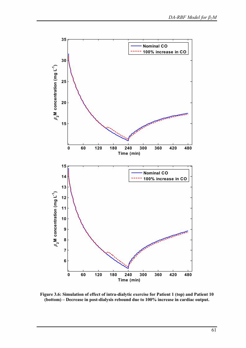
DA-RBF Model for β2M
61
Figure 3.6: Simulation of effect of intra-dialytic exercise for Patient 1 (top) and Patient 10 (bottom) – Decrease in post-dialysis rebound due to 100% increase in cardiac output.
0 60 120 180 240 300 360 420 480
15
20
25
30
35
Time (min)
β 2M c
once
ntra
tion
(mg
L-1)
Nominal CO100% increase in CO
0 60 120 180 240 300 360 420 480
6
7
8
9
10
11
12
13
14
15
Time (min)
β 2M c
once
ntra
tion
(mg
L-1)
Nominal CO100% increase in CO

Chapter 3
62
To compare their individual effect on toxin removal, increase in both factors is studied
independently. (i) The model is simulated for CO = 6 L min-1 (without exercise) and CO
= 12 L min-1 (with intra-dialytic exercise) keeping Kip constant. To simulate the toxin
kinetics during exercise, the HFR blood flow remained same as in no exercise condition
[85], thus rest of the increased cardiac output will perfuse LFR. (ii) To observe the effect
of increase in Kip, a hypothetical increase of 15% is studied (keeping cardiac output
constant at 6 L min-1). In all the cases, the post-dialysis rebound is calculated using the
following equation [72].
480 240
0 240
% 100C CReboundC C
−= ×
− (3.24)
Difference in percentage rebound is calculated for CO = 6 and 12 L min-1; similar
calculations are performed between nominal Kip and 15% increased Kip. Table 3.4
comprises the quantitative results corresponding to both scenarios. It is observed that 15%
increase in Kip can result in similar decrease as obtained with 100% increase in CO.
Hence, it can be concluded that intra-dialytic exercise not only increases the CO but also
increases the Kip. To substantiate this hypothesis, further clinical studies need to be
carried out so as to segregate the effect of CO and Kip on arterial toxin plasma
concentration, and formulating a relationship between the effect of exercise and toxin
removal. Such clinical studies can also help in quantifying the effect of exercise on inter-
compartmental clearance.

DA-RBF Model for β2M
63
Table 3.4: Simulating effect of intra-dialytic exercise – Decrease in rebound % (a) for 100% increase in cardiac output (CO) and (b) for 15%
increase in inter-compartmental mass transfer coefficient (Kip)
Patient
No.
Effect of increase in CO, keeping Kip constant Effect of increase in Kip, keeping CO constant
Rebound % during
normal dialysis
(CO = 6 L min-1)
Rebound % with
intra-dialytic exercise
(CO = 12 L min-1)
Decrease in
Rebound % due
to exercise
Rebound % during
normal dialysis
(Kip = nominal)
Rebound % with
intra-dialytic exercise
(Kip = 1.15 × nominal)
Decrease in
Rebound % due
to exercise
1 31.37 30.07 1.30 31.76 31.00 0.75
2 23.38 22.64 0.74 24.71 23.92 0.80
3 32.91 32.06 0.85 34.95 33.60 1.35
4 37.18 36.49 0.69 37.75 36.59 1.17
5 39.21 38.78 0.43 40.48 39.31 1.17
6 33.57 32.90 0.68 35.35 34.57 0.78
7 25.63 24.25 1.38 25.31 24.30 1.01
8 33.95 33.31 0.64 33.73 32.91 0.82
9 33.38 32.70 0.68 34.13 33.17 0.97
10 37.45 36.25 1.21 37.20 36.20 1.00

Chapter 3
64
3.6 Summary
A comprehensive model (diffusion-adjusted regional blood flow model) describing the
removal kinetics of middle-sized marker toxin, β2-microglobulin, has been presented.
Based on a priori identifiability analysis, the number of estimable parameters is reduced
from seven to three. The estimates for toxin distribution volume (Vd) are greater than
those obtained with two-compartment models, which can be justified by the fact that
patients on maintenance hemodialysis are fluid overloaded. Estimates of plasma fraction
in extracellular compartment (fP) suggest that more of this excess fluid stores in plasma
compartment, which explains the reason for renal patients being hypertensive. In
summary, the reduced parameter DA-RBF model results in improved understanding of
β2-microglobulin kinetics. The developed model results in higher estimate of removed
toxin mass than that obtained by the two-pool model. This information can be used to
validate the existing models and select the one that is the best representative of
physiology. To demonstrate the clinical application of the developed model, the effect of
intra-dialytic exercise is examined. Based on the simulation results, it is suggested that
increase in cardiac output alone cannot explain the decrease in rebound, and it is
hypothesized that stating that intra-dialytic exercise not only increases the cardiac output
but also increases the inter-compartmental mass transfer coefficient (Kip). When
combined together, both these manifests as lower post-dialysis rebound i.e. increased
toxin removal. Further clinical studies are required to study the effect of exercise on toxin
removal and to quantify the associated physiological changes. After confirming the intra-
dialytic exercise effect in prospective clinical trials, the developed model can be utilized
for systematic introduction of intra-dialytic exercise and synergizing its effect with
dialysis to obtain improved patient outcomes.

Clinical Study
65
4. Clinical Study to Compare Toxin Removal in Hemodialysis,
Hemodiafiltration, and Hemodialysis with Exercise§
“The strongest arguments prove nothing so long as the conclusions are not verified by
experience. Experimental science is the queen of sciences and the goal of all
speculation.”
- Roger Bacon
The previous chapter described a comprehensive model for β2-microglobulin kinetics.
Employing the developed model, the effect of exercise during dialysis was studied. To
explain the existing clinical evidence pertaining to enhanced toxin removal by exercise, it
is hypothesized that intra-dialytic exercise not only increases the perfusion of remote
body compartments, but also decreases the inter-compartmental resistance. To advance
further, clinical studies are required to test the proposed hypotheses. In this direction, a
pilot clinical research to investigate the effect of exercise during dialysis on toxin removal
is designed. The primary focus of this clinical research is to investigate the physiological
changes associated with intra-dialytic exercise.
As discussed in sub-section 1.3.2, hemodiafiltration (HDF) has also shown to improve the
toxin removal; hence, it is also studied for comparison purpose. The HDF details and
associated literature evidence are presented in Section 4.1. In Section 4.2, clinical
evidences for exercise and involved hypotheses are presented. The clinical trial design
aspects are presented in Section 4.3. Information on study patients and dialysis
§ A portion of this chapter has been published in: Vaibhav Maheshwari, Lakshminarayanan Samavedham, Gade Pandu Rangaiah, Yijun Loy, Lieng Hsi Ling, Sunil Sethi and Titus Lau Wai Leong. Comparison of toxin removal outcomes in online hemodiafiltration and intra-dialytic exercise in high-flux hemodialysis: A prospective randomized open-label clinical study protocol; BMC Nephrology, 13: 156, 2012

Chapter 4
66
prescription are provided in Section 4.4. The results and discussion are presented in
Sections 4.5 and 4.6, respectively.
4.1 Hemodiafiltration
According to single-pool assumption, the toxin removal is primarily hindered by dialyzer
membrane pore size. Hence, an easy maneuver for increasing the toxin removal is to
increase the membrane pore size. Two randomized clinical trials, Hemodialysis study and
Membrane Permeability Outcome study have shown the superiority of large pore size
membrane (high flux dialyzers) over small pore size membrane (low flux dialyzers) in
decreasing the mortality and morbidity [101, 102]. Nevertheless, the removal of middle-
sized toxins is poor with high-flux membranes, and CHD patients are often overloaded
with middle-sized uremic toxins. The reason is that toxin removal in CHD is primarily
controlled by diffusion. Since diffusion is inversely proportional to molecular weight or
size [103], removal of middle-sized toxins is relatively smaller than that of small-sized
toxins. Also, membrane pore size cannot be increased beyond certain limits because it
may translate in loss of important constituents of blood such as glucose, proteins, etc.
HDF augments the toxin removal by convection, which mobilizes the toxins and thus
enhances their removal. Understanding the toxin removal in dialyzer can clearly elucidate
the role of diffusion and convection in toxin removal. In TKM, the dialyzer performance
is quantified by dialyzer clearance (KD), which determines the removal rate. Following
Figure 4.1, the KD can be calculated as [46],
D Bi Bi Bi Bo BoK C Q C Q C= − (4.1)
where BiQ and BoQ denote blood flow at the inlet and outlet of dialyzer (mL/min), CBi
and CBo are corresponding concentrations of uremic toxin.

Clinical Study
67
Figure 4.1: Blood and dialysate flow along dialyzer length. Horizontal arrows represent transfer of accumulated toxins and excess fluid from blood to dialysate stream
Along the dialyzer length, fluid is removed at a certain rate. If the rate of fluid removal is
QF, then
Bo Bi FQ Q Q= − (4.2)
Replacing BiQ simply by BQ , equation 4.1 simplifies to a general formula for dialyzer
clearance,
Bi Bo BoD B F
Bi Bi
Bi BoD B F F
Bi
( )
C C CK Q QC C
C CK Q Q QC
−= +
−⇒ = − +
(4.3)
Hence, to calculate KD, blood samples at the inlet and outlet of dialyzer should be
collected. During dialysis, the membrane permeability would decrease thus KD will also
decrease; however, clinical studies found that KD remains almost constant during 4 hour
dialysis [46, 74]. The first term in equation 4.3 describes the effect of diffusion on toxin
removal and the second that of convection. In CHD, the fluid removal rate is 10-15
mL/min, which is decided based on the amount of weight gain during inter-dialysis
period. This is very small when compared with the diffusive component. In HDF, the QF
contribution is increased by removing excess fluid along dialyzer length, which is
Dialysate In
Dialysate Out
QBi
CBi
QBo
CBo
QF

Chapter 4
68
compensated by addition of sterile fluid before blood goes back to the patient. Typical
replacement fluid volume during 4 hour HDF process is ~20 L, which corresponds to QF
= 80 mL/min. The HDF can be performed in pre-dilution and post-dilution mode,
depending on the point of fluid infusion. Figure 4.2 schematically presents both modes of
HDF.
Figure 4.2: Pre- and post-dilution modes of hemodiafiltration. The given blood and dialysate flow rate are usual numbers practiced in routine dialysis settings. The replacement fluid rate is assumed to be 80 mL/min.
The utmost requirement of HDF is the availability of non-pyrogenic sterile replacement
fluid, which can be added to the blood stream. In the past, the replacement fluid was
provided in sterile bags, but the extremely high cost prohibited this practice. On-line
regeneration of replacement fluid has decreased this cost [104, 105], and resulted in
increased acceptability of HDF. This mode of HDF is known as online-HDF.
4.1.1 Clinical Evidences for HDF
HDF is increasingly being considered as superior to CHD, and is a subject of major
research [19, 106]. Numerous randomized controlled trials have studied its efficacy for
toxin removal and clinical outcomes [20, 107-111]. As discussed earlier, the basic
premise for encouraging HDF is the forced ultrafiltration rate that results in increased
QBi = 250 ml/min
QBo = 240 ml/min
QDi = 500 ml/min
QDo = 590 ml/min
80 ml/min
Post-dilution
QBi = 250 ml/min
QBo = 240 ml/min
80 ml/min
QDi = 500 ml/min
QDo = 590 ml/min
Pre-dilution
QBi = 250 ml/min
QBo = 240 ml/min

Clinical Study
69
removal of middle and large-sized toxins via convection [112, 113]. Despite numerous
documented benefits of HDF, there is lack of evidence from various clinical trials that
HDF can improve the toxin removal. This points to a need of properly designed
randomized controlled clinical trials [19, 114].
Among clinical trials studying HDF, a prospective clinical study comparing online-HDF
and high flux HD has shown that both small (urea and creatinine) and large (β2M and
complement factor D) sized toxin removal were greater for HDF when compared to high-
flux HD. However, this increased removal of urea and creatinine did not result in lower
pre-treatment serum concentration in both groups. In the context of large-sized molecules,
it was found that, after one year, pre-treatment serum β2M levels were similar in both
regimens, but significant decrease was observed for complement factor D [20].
Complement factor D is one of the toxins distributed in blood plasma. Based on these
evidences, it was concluded that efficacy of HDF is largely limited to blood compartment
only and is restricted by inter-compartmental resistance [74]. Toxins, which are
distributed in intracellular and/or interstitial compartments, in addition to blood plasma
compartment, are severely restricted by cellular membrane or capillary endothelium. This
also explained the significant removal of complement factor D, for its distribution is
limited to blood compartment only. Since majority of uremic toxins are distributed in
both IC and EC, HDF and high-flux HD seem to detoxify the blood compartment
primarily. These arguments also led to conclude that, after a certain volume of
replacement fluid in HDF, there will not be significant benefit for toxin removal, as blood
plasma compartment will almost be devoid of toxins and inflow of toxins from remote
compartments is restricted by inter-compartmental resistance. This explains why even
with very high volume of replacement fluid (60 L), there was no significant improvement
in toxin removal [115]. The only plausible way to overcome this resistance is to opt for
Chapter 4
70
intensive dialysis, i.e. prescribe long nocturnal dialysis or increased frequency of dialysis,
which have been found to be more efficacious than the high flux HD [57, 116].
In another clinical study performed on 20 subjects, removal outcomes of HDF and low
flux HD were compared for asymmetric dimethylarginine (ADMA), which is one of the
guanidino compounds. There was no benefit from HDF over HD in lowering the ADMA
concentration; rather, authors found that low-flux HD was superior in increasing the L-
arginine/ADMA ratio [117]. The reason for insignificant ADMA removal was associated
with protein binding of ADMA. However, it is noted that ADMA is a metabolic by-
product of protein modification process in human cells, thus it may also be chiefly intra-
cellular, and so HDF will be inefficient for its removal. This further strengthens the
conclusion of Ward et al. that inter-compartmental resistance is the major barrier for toxin
removal [74].
Recent Turkish online-HDF study [110] comparing high-flux HD and HDF observed
decreased incidence of cardiovascular mortality in patients with high amount of
replacement fluid. Nevertheless, the positive outcomes cannot be associated with
increased toxin removal in HDF because authors could not find statistically significant
difference in pre-dialysis serum concentration of urea, creatinine, phosphate, and β2M
after two years [110]. The superiority of HDF over conventional high-flux HD in long
term clinical trials is still debated [114], and this thesis does not intend to delve on this
debate. Rather, the intention here is to see – how we can further improve the toxin
removal performance of CHD or HDF by overcoming the physiological barrier. Exercise
during dialysis has been found to improve the toxin removal, although acceptance of
exercise intervention in clinical setting is poor.
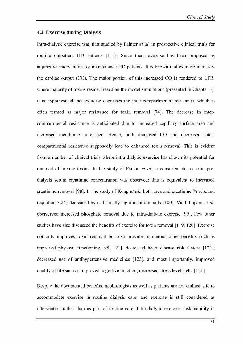
Clinical Study
71
4.2 Exercise during Dialysis
Intra-dialytic exercise was first studied by Painter et al. in prospective clinical trials for
routine outpatient HD patients [118]. Since then, exercise has been proposed as
adjunctive intervention for maintenance HD patients. It is known that exercise increases
the cardiac output (CO). The major portion of this increased CO is rendered to LFR,
where majority of toxins reside. Based on the model simulations (presented in Chapter 3),
it is hypothesized that exercise decreases the inter-compartmental resistance, which is
often termed as major resistance for toxin removal [74]. The decrease in inter-
compartmental resistance is anticipated due to increased capillary surface area and
increased membrane pore size. Hence, both increased CO and decreased inter-
compartmental resistance supposedly lead to enhanced toxin removal. This is evident
from a number of clinical trials where intra-dialytic exercise has shown its potential for
removal of uremic toxins. In the study of Parson et al., a consistent decrease in pre-
dialysis serum creatinine concentration was observed; this is equivalent to increased
creatinine removal [98]. In the study of Kong et al., both urea and creatinine % rebound
(equation 3.24) decreased by statistically significant amounts [100]. Vaithilingam et al.
oberserved increased phosphate removal due to intra-dialytic exercise [99]. Few other
studies have also discussed the benefits of exercise for toxin removal [119, 120]. Exercise
not only improves toxin removal but also provides numerous other benefits such as
improved physical functioning [98, 121], decreased heart disease risk factors [122],
decreased use of antihypertensive medicines [123], and most importantly, improved
quality of life such as improved cognitive function, decreased stress levels, etc. [121].
Despite the documented benefits, nephrologists as well as patients are not enthusiastic to
accommodate exercise in routine dialysis care, and exercise is still considered as
intervention rather than as part of routine care. Intra-dialytic exercise sustainability in

Chapter 4
72
routine HD setting is poor [124]. It will not be a mistake to say that exercise is one of the
most underrated clinical interventions in HD care. One reason behind this could be the
requirement of individualized prescription for intra-dialytic exercise [124]. Before we aim
for individualized prescription, it is important to understand what physiological changes
are responsible for enhanced toxin removal. In addition to increased CO and decreased
peripheral vascular resistance, exercise induced physiological changes may also occur
due to increased body core temperature. This is discussed in the following section.
4.2.1 Exercise and Temperature
It is hypothesized that exercise will increase the body core temperature which will further
dilate the blood vessels or vasculature, i.e. decrease the inter-compartmental resistance.
This hypothesis is based on results from another clinical research which studied the effect
of dialysate temperature on urea removal and patient hemodynamic stability [125].
Dialysate temperature plays an important role in patient hemodynamic stability and
conventional dialysate temperature is set at 36°C or 36.5°C, while body core temperature
is presumably 37°C. In the study of Kaufmann et al. comprising 15 HD subjects, effect of
cool dialysate (35.5°C) and thermo-neutral dialysate (37°C) was studied. It was noted that
cooled dialysate decreased the body core temperature by 0.22 ± 0.04 °C, while thermo-
neutral dialysate increased it by 0.31 ± 0.05 °C. The increase in body core temperature in
thermo-neutral dialysate was associated with inflammatory response. The cool dialysate
provided better hemodynamic stability. Nevertheless, cooling also resulted in ~400%
increase in peripheral vascular resistance index, when compared with thermo-neutral
dialysate. Interestingly, increased peripheral vascular resistance index did not affect the
urea removal and % rebound was similar in both cool and thermo-neutral dialysate [125].

Clinical Study
73
Peripheral vascular resistance index, also known as systemic vascular resistance index,
can be considered as surrogate of inter-compartmental resistance. Increased peripheral
vascular resistance index could not affect the urea removal, because urea is small in size
and its kinetics is primarily flow controlled (Sub-section 2.3.4) [84]. Also, rapid
equilibration of urea across the cell membrane is essentially due to facilitated transport by
selective urea transporters [126]. This suggests that, even with vasoconstriction, urea can
easily pass through the cellular membrane and its removal is not affected. However, the
conclusion should not be extrapolated to other uremic toxins, and their removal may be
compromised in cool dialysate.
It is known that exercise increases the body core temperature due to increased oxygen
uptake and increased metabolism in cells [127]. To decrease the body core temperature or
to remove the accumulated heat, the blood flow to skin increases, and the person sweats.
In the context of HD subjects under intra-dialytic exercise, this increased blood flow will
mobilize toxins from remote compartments. However, there is no clinical study to
investigate the effect of intra-dialytic exercise on body core temperature. It is
hypothesized that exercise will increase the body core temperature, which will decrease
the inter-compartmental resistance and result in increased toxin removal. To study change
in peripheral vascular resistance index, patients were subjected to echocardiogram during
the exercise session.
4.3 Clinical Trial Design
Following the preceding discussion, the proposed clinical trial was aimed to investigate
the exercise induced physiological changes. The inter-compartmental resistance cannot be
measured, and so change in peripheral resistance index is used as surrogate. The
resistance index is measured via echocardiogram, also referred as Doppler ultrasound,

Chapter 4
74
which is a non-invasive way to quantify the physiological changes (see Sub-section
4.3.4). The specific aims of study are:
1. Investigate the effect of intra-dialytic exercise on physiological changes, namely,
decrease in inter-compartmental resistance, increase in CO, and increase in body
core temperature due to exercise. The decrease in inter-compartmental clearance
will be assessed by decrease in peripheral vascular resistance index.
2. Investigate the effect of intra-dialytic exercise on removal of middle molecule
marker toxin, β2-micorglobulin and compare the same with CHD and HDF. This
is the first study to investigate the effect of exercise on β2-micorglobulin removal.
The toxin removal outcome will be assessed by 2 hour post-dialysis % rebound.
The rebound % will also be compared for conventional toxins: urea, creatinine,
and phosphate.
4.3.1 Study Design and Ethics Approval
This study was single center, open label, self-controlled (within subject design),
randomized prospective, efficacy study involving patients undergoing conventional high-
flux HD. Blinding is an important aspect for randomized study; this helps in preventing
the investigator and subject bias. However, blinding was not feasible because the changes
in conventional HD are immediately visible to both study subjects and investigators.
The domain specific review board affiliated with the National Healthcare Group (NHG),
Singapore has approved the trial. The study has undergone routine quality assurance
review conducted by the ethics board. The ethics board also received timely progress
status report and promptly informed of any adverse events owing to the intervention
during the course of the study. The study was conducted at outpatient dialysis center of
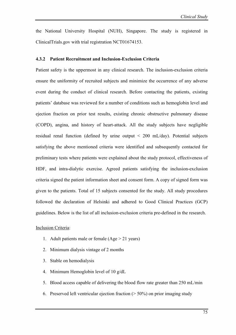
Clinical Study
75
the National University Hospital (NUH), Singapore. The study is registered in
ClinicalTrials.gov with trial registration NCT01674153.
4.3.2 Patient Recruitment and Inclusion-Exclusion Criteria
Patient safety is the uppermost in any clinical research. The inclusion-exclusion criteria
ensure the uniformity of recruited subjects and minimize the occurrence of any adverse
event during the conduct of clinical research. Before contacting the patients, existing
patients’ database was reviewed for a number of conditions such as hemoglobin level and
ejection fraction on prior test results, existing chronic obstructive pulmonary disease
(COPD), angina, and history of heart-attack. All the study subjects have negligible
residual renal function (defined by urine output < 200 mL/day). Potential subjects
satisfying the above mentioned criteria were identified and subsequently contacted for
preliminary tests where patients were explained about the study protocol, effectiveness of
HDF, and intra-dialytic exercise. Agreed patients satisfying the inclusion-exclusion
criteria signed the patient information sheet and consent form. A copy of signed form was
given to the patients. Total of 15 subjects consented for the study. All study procedures
followed the declaration of Helsinki and adhered to Good Clinical Practices (GCP)
guidelines. Below is the list of all inclusion-exclusion criteria pre-defined in the research.
Inclusion Criteria
1. Adult patients male or female (Age > 21 years)
:
2. Minimum dialysis vintage of 2 months
3. Stable on hemodialysis
4. Minimum Hemoglobin level of 10 g/dL
5. Blood access capable of delivering the blood flow rate greater than 250 mL/min
6. Preserved left ventricular ejection fraction (> 50%) on prior imaging study

Chapter 4
76
7. Desirable performance in 6-min walk test (6 MWT)
Exclusion Criteria
1. History of recurring or persistent hypotension in the past 2 months
:
2. Pregnant woman
3. Severely Hypertensive patients (systolic blood pressure > 180 mmHg and/or
diastolic blood pressure > 115 mmHg)
4. History of recent myocardial infarction or unstable angina (within the past 6
months)
5. Significant valvular disease, i.e. severe aortic stenosis and moderate-severe mitral
regurgitation.
6. Patients with end stage organ disease e.g. COPD, recent or debilitating
cerebrovascular accident (CVA)
7. Patient with recent stroke (within the past 6 months)
8. Anemic patients
9. History of known arrhythmia
10. Participation in another clinical intervention trial
11. Moderate to severe osteoarthritis of knee(s)
12. Unable to consent
The consented subjects were called for 6 MWT, which was performed according to the
standard guidelines prescribed by American Thoracic Society [128]. This test has been
considered as appropriate sub-maximum test to assess patient’s functional and
physiological response, cardiovascular fitness, and suitability for intra-dialytic exercise in
ESRD population [129]. Patients walked along a measured circuit (30 m), instructed to
cover as much distance as they can within 6 min. Patients were not allowed to run. Blood

Clinical Study
77
pressure (BP), heart rate (HR) and rate of perceived exertion (RPE) were assessed at pre-
and post- 6 MWT. HR and RPE were measured at every minute of the test, as well as at 8
and 10 min to assess heart rate recovery (HRR) and blood pressure. Patients who
ambulated less than 300 m over 6 min were excluded from the test due to the likelihood
that they may not tolerate the exercise protocol (described in Sub-section 4.3.4). Patients
were also supposed to demonstrate acceptable physiological response during the test, e.g.
HRR, hemodynamic parameters within safe guidelines for exercise. The 6 MWT was
conducted by a trained physiotherapist.
4.3.3 Study Interventions
All recruited study subjects underwent three different study dialysis sessions, namely,
HD, HDF, and HD with intra-dialytic exercise (HD-Ex) within a maximum time interval
of 6 months between the first and last study session. Minimum one week gap was
maintained between study sessions for each individual patient. The one-week gap should
remove any carry-over effect of previous study session and bring the patients to their
nominal toxin concentration level. High-flux HD was conducted as per the patient routine
dialysis session; HDF was conducted with 18 L of target replacement fluid. Patients’
medications such as phosphate binder, medication for hypertension, erythropoietin dose,
etc. were not changed during the study period. Patients were also advised to keep their
diet fairly constant during the study period. The study sessions were conducted in mid-
week or end-week setting; however, study sessions for an individual subject were on the
same day of the week. To avoid the effect of confounding factors, same dialysis
conditions were used in all study dialysis sessions.
The intra-dialytic exercise was conducted in conventional high-flux HD setting with
exercise prescription in three bouts. The first exercise bout started from 40–60 min,

Chapter 4
78
second from 80–100 min, and third from 120–140 min. If patients were unable to adhere
to the prescribed exercise intervention, then they were advised to perform a total of 60
min exercise during the dialysis. The exercise was sustained till the achievement of 70%
of maximum heart rate, and given via active cycling movement (ACM) using calibrated
Monark 881E cycle ergometer (Monark, Sweden). The maximum heart rate is calculated
by subtracting patient age from 220. Various hemodynamic responses, namely, heart rate,
blood pressure, arterial and venous blood temperature were measured during all study
sessions. Additional hemodynamic responses, namely, CO and peripheral vascular
resistance index, were also assessed by measuring left ventricular stroke volume using
Doppler echocardiography. The echocardiogram images were taken just before starting of
HD-Ex session, before starting first bout of exercise, at 5-minute intervals during
exercise, and after termination of first exercise bout. But they were not taken during the
second and third bouts of exercise because similar cardiac responses were anticipated.
Systemic vascular resistance and parameters of ventricular-arterial coupling were derived
to determine the stroke volume response to exercise. The echocardiography was also used
to assess cardiac structure and function before and during exercise – any new or
unexpected abnormality, e.g. regional dysfunction. Any abnormality was recorded and
best possible clinical judgment was taken to ensure patient safety. If during exercise,
patient’s systolic blood pressure exceeds beyond 180 mm Hg, the patient was asked to
stop exercise till the pressure attains the safe level of below 180 mm Hg.
4.3.4 Data collection
Blood sampling
Three arterial blood samples, namely, pre-dialysis (t = 0 min), end-dialysis (t = 240 min),
and post-rebound (t = 360 min) were collected in each study session. Each blood sample
:

Clinical Study
79
was analyzed for uremic toxins, namely, urea, creatinine, phosphate, and β2M. The
volume of each collected blood sample was ~4 mL. All the blood samples were sent to
NUH clinical laboratory immediately after collection. These toxins/solutes concentrations
were used for calculating the post-dialytic % rebound for each toxin. Conventionally, the
blood samples are collected in tubes containing EDTA, which is a strong anticoagulant
[74]. The anticoagulant prevents the blood clotting. This practice can plausibly equilibrate
the toxin concentration between blood cells and plasma. However, as discussed earlier
(Figure 3.5), dialysis process results in the concentration gradient between inaccessible
cellular/interstitial compartments and accessible blood compartment. To prevent the
concentration equilibration, all blood samples were collected in serum separator tubes
(SST II), also referred as gold cap tubes. These tubes are coated with clot activator which
expedites the blood clotting. The faster blood clotting prevents the equilibration of toxin
among blood plasma and blood cells. The gel inside SST II tubes separates the blood
plasma and blood cells, so that plasma extraction after centrifugation becomes relatively
easier.
Blood temperature monitoring
Arterial and venous blood temperature was continuously monitored using blood
temperature monitor, abbreviated as BTM (Fresenius, Bad Homburg, Germany). As
discussed earlier, intra-dialytic exercise will increase the body core temperature (Sub-
section 4.2.1). The dialysate temperature directly affects the blood temperature; hence, it
was kept same for all three study sessions for each individual patient. The dialysate
temperature was measured during HD-Ex session alone. During standard HD or HDF, the
blood temperature change is insignificant (Figure 4.3); hence, during these sessions,
blood temperature was not measured. The schematic flow chart of clinical trials is
:

Chapter 4
80
presented in Figure 4.4. To maintain patient confidentiality, all the collected samples and
data were assigned a unique study number.
Figure 4.3 Blood temperature snapshot during HD session for two sample patients. In panel A, the kink in dialysate and venous temperatures is due to the measurement of access recirculation.
4.4 Patient and Dialysis Information
A total of 15 patients consented to participate in the study. Two patients could not fulfill
the inclusion-exclusion criteria. Information pertaining to individual subjects who
underwent the study intervention is provided in Table 4.1. Among 13 patients, one patient
was prohibited to continue on HD-Ex session owing to poor baseline ejection fraction
(25%); according to the inclusion-exclusion criteria, the baseline ejection fraction should
be at least 50%. To prevent any adverse event, this particular patient was not allowed to
undergo HD-Ex session. Hence, a total 38 study sessions were performed. Among the 12
patients who completed all 3 study sessions, echocardiogram could not be performed for
one subject. Nevertheless, exercise intervention was followed as per the protocol

Clinical Study
81
discussed in Sub-section 4.3.3 and blood samples were collected as per the protocol
discussed in Sub-section 4.3.4.
Table 4.1: Patient demographics at the time of consent
Patient ID
Gender Age Hemoglobin (mg/dL)
Ejection fraction (on prior imaging)
Distance covered in 6 MWT (m)
P1 M 51 11.6 74 470
P2 M 66.5 13.9 75 460
P3 F 42 10.1 67 360
P4 M 55 12.7 56 423
P5 M 56 12.7 61 510
P6 F 63 12.6 72 368
P7 M 52 12 56 405
P8 F 40.5 11.6 58 425
P9 F 42 12.7 54 375
P10 F 55 11.5 55 397
P11 M 56 11.2 61 430
P12 F 54 11.4 55 570
P13 M 23 11.6 72 576
Mean ± std 50.5 ± 11.3 12 ± 0.95 63 ± 8 % 444 ± 71
All HD and HD-Ex sessions were conducted on Fresenius 4008S, and HDF sessions were
performed on Gambro AK200. The dialyzer was same in all study sessions for an
individual patient. All dialysis related parameters such as dialysate temperature, dialysate
composition, were kept same in the study sessions of an individual patient to minimize
the confounding factors. However, the ultrafiltration or fluid removal rate during each
study session was calculated based on inter-dialytic weight gain, and was different for
different sessions. It is assumed that excess fluid removal via ultrafiltration will
insignificantly contribute towards toxin removal. The mean convective fluid volume in
HDF was 21.2 ± 3.7 L, with minimum and maximum at 15.8 and 29.1 L, respectively.

Chapter 4
82
Figure 4.4: Schematic flow-chart of clinical trial
Identify mobile subjects:- Obtain list of mobile patients- Access mobile patients’ existing clinical history- Check for existing cardiovascular and/or
orthopedic diseases
Explain to the identified subjects:- Satisfying inclusion-exclusion criteria- Information on intra-dialytic exercise and HDF- Post-dialysis stay for 2 hours- Blood sampling- Echocardiogram in intra-dialytic exercise study- Information about 6 min-walk-test - Report all relevant study results
Consent and 6 min-walk-test- Obtain patient consent in the presence- Perform 6 min-walk-test
Study visit 0
Educating identified subjects
Pre-recruitment
process
Random allocation of dialysis sessions – Study visit 1/2/3
3 study sessions per patient in random order• High-flux Hemodialysis (HD)• Hemodiafiltration (HDF)• HD with intra-dialytic exercise (HD-Ex)
• Collection of arterial blood samples• Analysis of collected samples for urea,
creatinine, phosphate, sodium, potassium, and β2-microglobulin
• Perform ultrasound echocardiography (HD-Ex)• Measure blood temperature using BTM (HD-Ex)
Sampling, analysis, and
Data collection
Data analysis
Primary outcome measure Compare % rebound outcomeSecondary outcome measure Study change in peripheral vascular
resistance index and temperature

Clinical Study
83
4.5 Results from the Clinical Study
The toxin removal is adjudged by % rebound calculation. The mean % rebound in HD,
HDF, and HD-Ex for uremic toxins: urea, creatinine, phosphate, and β2M are presented in
Table 4.2. The rebound was calculated using pre-dialysis (t = 0 min), end-dialysis (t =
240 min), and post-rebound (t = 360 min) plasma toxin concentration (equation 3.24).
Table 4.2: Percentage rebound for each uremic toxin in different dialysis protocols
Dialysis Protocol Urea Creatinine Phosphate β2-microglobulin
HD 13.4 ± 3.3 22.7 ± 4.2 37 ± 8.1 29.1 ± 14.5
HDF 14.4 ± 5.4 22.8 ± 4.5 23.5 ± 16.5 24.5 ± 3.0
HD-Ex 13.5 ± 4.0 22.0 ± 3.6 52.1 ± 21.6 27.4 ± 5.9
In Table 4.2, the mean % rebound results for HD corresponds to 12 patients. For one
patient, the post-rebound sample was corrupted due to dilution while sampling blood. For
HDF, phosphate rebound for one patient was negative because the post-dialysis phosphate
concentration was lower than the end-dialysis concentration, which seems unrealistic.
This was considered as wrong phosphate concentration measurement; thus the phosphate
% rebound calculation in HDF is from 12 patients. Similarly, the % rebound presented for
HD-Ex is based on 12 patients, as one patient was not allowed to continue with the
exercise due to poor baseline ejection fraction.
The blood temperature profiles during HD-Ex session are presented in Figure 4.5, where
three peaks in arterial blood temperature can be observed. These three peaks correspond
to three bouts of exercise. On the other hand, insignificant changes are seen in venous
temperature. Small variations in venous temperature can be attributed to fluctuations in
dialysate temperature. Notably for P6, the arterial temperature does not reflect in exact

Chapter 4
84
three peaks, rather four small peaks can be observed. This is because patient completed
the prescribed exercise protocol in four bouts. The venous temperature for the same
patient P6 is also perturbed due to unexpected change in dialysate temperature. The
difference between maximum and minimum arterial temperature was 0.96 ± 0.23 °C. The
variation denotes the inter-patient variability, i.e. each patient hemodynamic response is
different to exercise intervention. Also the intensity of exercise was not controlled, and
patients exercised at their comfort levels.
The results for change in cardiac output and peripheral vascular resistance index for
individual patients are presented in Figure 4.6. Although patients started the exercise bout
at different times (Figure 4.5), it is assumed that all patients started their first exercise
bout at 40 min during dialysis. This assumption is made to standardize the change in CO
and resistance index for all patients. The mean increase in CO is 4.34 ± 1 L/min, while
mean decrease in resistance index is 874 ± 272 dyn.s/cm5. The mean maximum-
percentage increase in CO is 106 ± 32%, with maximum and minimum increment being
147% and 61%, respectively. Similarly, the mean maximum-percentage decrease in
resistance index is 94 ± 45%, with maximum and minimum reduction being 186% and
42%, respectively.

Clinical Study
85
Figure 4.5: Arterial (red - -) and Venous (blue - -) blood temperature during HD-Ex session
0 50 100 150 200 25034.5
35.0
35.5
36.0
36.5
37.0
37.5
50 100 150 200 250
35.0
35.5
36.0
36.5
37.0
37.5
38.0
0 50 100 150 200 25034.5
35.0
35.5
36.0
36.5
37.0
37.5
38.0
0 50 100 150 200 25034.535.035.536.036.537.037.538.0
0 50 100 150 200 25034.535.035.536.036.537.037.538.0
0 50 100 150 200 25035.0
35.5
36.0
36.5
37.0
37.5
0 50 100 150 200 25035.0
35.5
36.0
36.5
37.0
37.5
38.0
0 40 80 120 160 200
35.5
36.0
36.5
37.0
37.5
50 100 150 200 250
35.5
36.0
36.5
37.0
37.5
0 50 100 150 200 250
35.5
36.0
36.5
37.0
37.5
38.0
0 50 100 150 200 250
35.5
36.0
36.5
37.0
37.5
0 50 100 150 200 250
35.0
35.5
36.0
36.5
37.0
37.5
P1 P2 P3 P4
P5 P6 P7
P8
Time on Dialysis (min)
Arte
rial a
nd V
enou
s Blo
od T
empe
ratu
re (o C
)
P9 P11 P12 P13

Chapter 4
86
Figure 4.6: Patients' cardiac output and peripheral vascular resistance index during the first bout of exercise. In bottom panel, cardiac
output and resistance index are presented as mean ± standard deviation.
0 20 40 60 80
3
4
5
6
7
8
9
10
0 20 40 60 80
500
1000
1500
2000
2500
3000
0 20 40 60 803
4
5
6
7
8
9
10
0 20 40 60 80600
800
1000
1200
1400
1600
1800
2000
2200
2400
Card
iac O
utpu
t (L/
min
)
P2 P3 P4 P5 P6 P7 P8 P9 P11 P12 P13
Resis
tanc
e Ind
ex (d
yn.s/
cm5 )
Card
iac O
uput
(L/m
in)
Resis
tanc
e Ind
ex (d
yn.s/
cm5 )

Clinical Study
87
4.6 Discussion
In this study, the toxin removal is adjudged by % rebound after dialysis. Comparison of
% rebound in different dialysis protocols will prove the efficacy of one over another. It
should be noted that magnitude of % rebound and time required for equilibration in body
compartments can be different for different toxins, e.g. % rebound of large-sized toxins
can be more pronounced due to slower diffusion of large-sized molecules. In this clinical
study, it was assumed that toxins will equilibrate within two hours post-dialysis and
rebound will recede thereafter. Comparing the urea rebound values in Table 4.2, it can be
observed that mean % rebound is comparable among HD, HDF, and HD-Ex, except HDF
results in slightly larger mean % rebound. These results suggest that urea removal is
primarily controlled by diffusion and is not affected by convection, which is the
augmented characteristic of HDF. The reason for slightly larger % urea rebound in HDF
is unknown, but may be ascribed to interference between diffusion and convection [130].
Toxin removal via convection is dependent on fluid transport from blood to dialysate
steam, i.e., it is independent of concentration gradient. Increased removal of fluid in HDF
will plausibly move more urea into dialysate stream and decrease the urea concentration
difference between blood and dialysate stream, and thus hamper the diffusive urea
transport. The assumption in this argument is that there is sufficient amount of toxin in
blood plasma compartment and there is no or insignificant resistance between
physiological compartments. Urea conforms to this assumption because urea is small in
size and inter-compartmental urea transport is boosted by urea transporters in cellular
wall. For other small as well as large-sized uremic toxins, no such specific transporters
exist on the cellular wall, and their removal is restricted by inter-compartmental
resistance. This is evident from % rebound results for creatinine. The mean % rebound of
creatinine is almost the same for both HD (22.7 %) and HDF (22.8 %), but is slightly

Chapter 4
88
lower for HD-Ex (22.0 %). The similar creatinine rebound from HD and HDF points out
to the similar contribution of diffusion and convection towards creatinine removal from
blood to dialysate stream. However, physiological resistance still plays the dominant role,
which is reduced by exercise. The slight drop in creatinine rebound in HD-Ex can be
associated with increased blood flow to remote peripheral compartments during exercise
and decreased peripheral resistance, quantified by resistance index (Figure 4.6).
The mean % rebound for β2M is lowest in HDF (24.5 %), which suggest that removal of
large-sized toxins is significantly contributed by convection. At the same time, the mean
% rebound of β2M in HD-Ex was 27.4 % which is lower than that obtained in HD
(29.1%). This indicates that, even without convection (i.e., with diffusion alone), the %
rebound can be reduced (i.e. toxin removal can be increased). These results suggests that
exercise can not only augment the removal of small-sized toxins [120], but also has
potential to increase the removal of large-sized uremic toxins. Comparing the toxin
removal outcomes for urea, creatinine, and β2M, it can be inferred that urea removal in
dialyzer is influenced by diffusion alone, creatinine removal is influenced by both
diffusion and convection, and β2M removal is primarily influenced by convection.
Interestingly, the mean % rebound for phosphate is significantly pronounced in HD-Ex
(52.1%) than that obtained in HD (37%) and HDF (23.5%). Vaithilingam et al. have
found that intra-dialytic exercise increases the phosphate removal [99]. The unexpected
high phosphate rebound in the present clinical study can only be explained by
significantly delayed mobilization of phosphate from bones or remote intracellular
compartments, which manifests much after completion of dialysis. It is important to note
that in this study, the first exercise bout was implemented on or after 40 min from the
start of dialysis, but in the study of Vaithilingam et al. the exercise intervention was
before and/or during early phase of dialysis [99]. This suggests that exercise does increase

Clinical Study
89
the phosphate removal, but delayed mobilization can be the root cause of pronounced
rebound in this study. In other words, the post-dialytic wait of 2 hours is too small for
complete equilibration of phosphate, i.e. the rebound of phosphate may be delayed by as
much as 4 hours. In summary, to improve the phosphate removal, immediate pre-dialysis
exercise intervention may be more helpful than the intra-dialytic exercise intervention.
The important question then is whether this is true for all uremic toxins or only for
phosphate whose kinetics is most complex among all studied uremic toxins [56, 69]?
At the same time, the % rebound for phosphate is lowest in HDF, but prolonged HDF
interventions could not decrease the pre-dialysis phosphate concentration than that
obtained in high-flux HD [110]. If HDF reduces the phosphate rebound to such great
extent as observed in this pilot study then why it does not reflect in reduced pre-dialysis
serum phosphate concentration? This can be attributed to the fact that the efficacy of HDF
is primarily restricted to blood compartment only [74]. During 4h dialysis, the HDF will
plausibly decrease the plasma phosphate concentration to very low levels. Post-dialysis,
the phosphate rebound does occur but the 2h rebound period may be too small to see the
significant phosphate rebound. To further strengthen the above mentioned claims, more
clinical studies should be designed where patients should be asked to wait for 4h post-
dialysis. However, this is difficult and inconvenient for many patients. The other method
to adjudge the superiority of one dialysis protocol over another will be to collect the
whole spent dialysis and analyze a representative sample for removal of total toxin mass.
This is the first clinical study to investigate the effect of exercise on body core
temperature. As hypothesized, the intra-dialytic exercise results in increase in body core
temperature which was inferred from measured arterial blood temperature. In Figure 4.5,
three distinct peaks can be observed which correspond to three successive bouts of
Blood Temperature and Hemodynamic Response

Chapter 4
90
exercise. Although all recruited patients were unconditioned to exercise, all of them were
able to complete the 60 min exercise intervention without any adverse event requiring
clinical intervention. The key reason for this is that the exercise protocol was performed
at zero resistance, which was easily tolerated by this cohort of patients. The venous
temperature is almost constant throughout the dialysis sessions (Figure 4.5), because inlet
(arterial) blood comes in contact with dialysate which is at constant temperature. Within
the length of dialyzer module, the heat transfer from inlet blood to dialysate stream will
bring the outlet (venous) blood to the dialysate temperature. However, the venous blood
temperature is always lower than the dialysate temperature. This is because, after exiting
from the dialyzer, the venous blood circuit comes in contact with environmental
temperature, which is much lower than the dialysate temperature. This environmental
heat loss plausibly decreases the venous blood temperature below dialysate temperature.
During HD-Ex session, patient’s cardiac output was also measured during the first bout of
exercise using Doppler echocardiogram. As expected, the patient’s CO peaks during
exercise intervention (Figure 4.6). At the same time, the vascular resistance index reached
the nadir during exercise. The decrease in peripheral resistance index can be attributed to
increased CO as well as increased blood core temperature, which results in increased
blood flow to remote compartments so that the excess heat can be removed via skin. It
remains unclear that between CO and temperature which one is the dominant factor for
decreasing the peripheral resistance. Nevertheless, without delving into the contribution
from individual factors, it is ascertained that exercise increases the body core temperature
(besides cardiac output) and decreases the inter-compartmental resistance which
eventually results in enhanced toxin removal.
Notably, the baseline (t = 0) CO drops from 5.41 ± 0.97 L/min to 4.62 ± 1.19 L/min just
before the start of exercise (t = 40 min), which is equivalent to ~15% decrease in CO.

Clinical Study
91
This can be attributed to the reduced venous blood temperature, which is much lower than
the arterial or systemic blood temperature (Figure 4.3). The systemic blood temperature
decreases, when cooled venous blood mixes with the systemic circulation. To reconcile
for this sudden decrease in blood temperature, the vasoconstriction occurs which reduces
the blood flow to remote compartments or manifest in the form of decreased cardiac
output. The vasoconstriction prevents the heat loss from skin or peripheral organs.
Although increased body core temperature may lead to incidence of intra-dialytic
hypotension, increased core temperature induces the blood flow to remote peripheral
compartments so that the body core temperature can be reduced. In the process, the
central blood volume decreases which can potentially result in IDH episode. The same
principle is used to achieve the hemodynamic stability via cool dialysate. Nevertheless, in
the present clinical tests, no episode of IDH requiring clinical intervention was
experienced. This can be credited to the inclusion-exclusion criteria which prevented the
IDH prone patients to participate in the clinical study. The IDH prone patients were
prevented to participate because the objective here was to compare the physiological
changes and toxin removal, rather than to test the compliance of IDH prone patients on
exercise intervention.
One should note that, among the four studied uremic toxins, % rebound is highest for
phosphate. Although phosphate is much smaller in size than β2M, its rebound is much
more pronounced. This is because phosphate is distributed in both IC and EC, but β2M is
distributed in EC alone. Additionally, the phosphate mobilization can occur from
pathologic stores of phosphate in bones. Following the model of Spalding et al. to explain
phosphate kinetics [56], the phosphate mobilization need to overcome at least three
Is β2-microglobulin an appropriate marker?

Chapter 4
92
physiological resistances – the first resistance when phosphate mobilizes from bone
matrix to cellular compartment, the second resistance by cellular membrane when
phosphate mobilizes from IC to EC, and the third resistance by capillary endothelium
when phosphate mobilizes from interstitial space to accessible blood compartment. On
the other hand, β2M, distributed in EC has to overcome only one resistance due to
capillary endothelium. Multiple resistances delay the phosphate removal and eventually
manifest in significantly high post-dialytic rebound. Although most uremic toxins do not
behave like phosphate, these toxins are still distributed in both IC and EC, and experience
at least two resistances by cellular membrane and by capillary endothelium. This
questions the credibility of β2M being designated as potential marker toxin instead of
conventional marker urea. Urea cannot be the marker because its removal kinetics does
not even coincide with other small-sized uremic toxins [67]. At the same time, caution
should be exercised before β2M is authoritatively accepted as the marker of toxin milieu.
Historically, urea is considered as marker toxin because of its high plasma concentration
and low cost of analysis, which seems to have played an important role in favoring urea
as marker toxin [25]. Hence, not only the toxin distribution but also the cost of analysis
should be considered while deciding a better representative of uremic toxins.
4.7 Summary
This is the first pilot clinical study to investigate the exercise induced physiological
change(s) responsible for enhanced toxin removal. It is also perhaps the first one that
compares the toxin removal outcome for both small and middle-sized toxins. The toxin
removal outcomes are compared for HD, HDF, and HD-Ex. The urea rebound is higher in
HDF, while creatinine rebound in HD-Ex is slightly lower than that obtained in HD or
HDF. The β2M rebound is lowest for HDF, but HD-Ex still results in lower rebound than
HD. These results indicate that it is more important to focus on patient physiology i.e.

Clinical Study
93
overcoming the inter-compartmental resistance rather than focusing on improvement of
RRTs. The rebound for phosphate (true to its complex kinetics) was highest in HD-Ex,
which is attributed to delayed mobilization of phosphate from remote bone matrix to
blood compartment. Results demand for an optimal exercise intervention for enhancing
the removal of phosphate as well as other uremic toxins. Note that the obtained results are
based on single session study on patients unconditioned to exercise. With prolonged
exercise intervention, it can be hypothesized that intra-dialytic exercise will culminate in
improved physical function or improved performance towards exercise. Patients will be
able to tolerate higher resistance exercise protocol which will further increase the toxin
removal. Long term clinical studies comparing the toxin removal in HDF and HD-Ex are
required to test the proposed hypotheses. With the obtained results, it can be proposed
that exercise during HDF can improve the removal of both small and large uremic toxins.
The present clinical study also proves that exercise intervention not only increases the
cardiac output but also increases the body core temperature which potentially decreases
the vascular resistance. Note that the decrease in vascular resistance is only an indication
towards reduced cellular resistance. It is impossible to measure the changes in inter-
compartmental resistance. To quantify the decrease in compartmental resistance,
previously discussed diffusion adjusted regional blood flow model (Chapter 3) can be
employed. The increase in inter-compartmental clearance (Kip, model parameter) can
quantify the decrease in inter-compartmental resistance. This requires the precise
estimation of Kip, which requires appropriate experimental data. The next part of the
thesis deals with experimental design aspects that lead to enhancing the precision of
estimates model parameters.


Part 2
Model-based Design of Experiments

Chapter 5
96
MOO based DOE
97
5. Multi-Objective Framework for Model-based Design of
Experiment Techniques§
Conflict is the beginning of consciousness.
- Mary Esther Harding
In Part 1, a comprehensive toxin kinetic model for β2-microglobulin was proposed. The
model was subsequently employed to explain the effect of exercise and new hypotheses
were proposed. To test the hypotheses, a pilot clinical study was carried out. The clinical
study validated the hypotheses that exercise during dialysis increases the toxin removal
by decreasing the inter-compartmental resistance. It also appears that decrease in inter-
compartmental resistance is not only due to increased cardiac output which dilates the
vasculature but also due to increased body core temperature which further dilates the
vasculature. However, the clinical study did not quantify the decrease in inter-
compartmental resistance. Quantifying the decrease in this resistance can provide a better
understanding of exercise induced physiological changes and pave way for personalized
prescription of intra-dialytic exercise. The model parameter Kip that characterizes the
inter-compartmental clearance can quantify the decrease in this compartmental resistance.
To estimate Kip, blood samples need to be collected. The important question addressed in
Part 2 of this thesis is related to the timing of collection of those samples so that Kip and
other model parameters can be precisely estimated. Towards this end, model-based design
of experiment (MBDOE) techniques can play an important role.
Before getting into the implementation details of MBDOE techniques for elucidating the
optimal HD sampling protocol, the importance of experiments and MBDOE paradigm are
§The contents of this chapter have been published in: Vaibhav Maheshwari, Gade Pandu Rangaiah, Lakshminarayanan Samavedham, Multi-objective framework for model-based design of experiments to improve parameter precision and minimize parameter correlation, Industrial and Engineering Chemistry Research, 52, 8289-8304 (2013).

Chapter 5
98
reviewed. It is observed that existing MBDOE techniques such as D-, A-, and E-optimal
designs have inherent drawbacks, which can potentially lead to poor precision of model
parameters and so defeats the objective of optimal experimental design. To overcome
these drawbacks, a new strategy is proposed and evaluated on two case studies.
5.1 Mathematical Models and Experiment
Mathematical models for processes form the foundation for their performance
improvement through optimization, control of product quality within pre-specified limits,
developing soft sensors for predicting and monitoring “difficult to measure” states, in
silico testing of new strategies, and/or for the development of new products/processes.
Success of all these activities relies significantly on precise and accurate description of
the system in the form of mathematical equations. Therefore, building a high-fidelity
model is a crucial step before employing the model as a proxy to the real system.
Model building can be regarded as an iterative process: starting with the objective of
model building, followed by a priori process knowledge in the form of physical,
chemical, or biological laws governing the system, preliminary tests, and initial
hypotheses; then a model structure in the form of algebraic equations (AEs), differential-
algebraic equations (DAEs), or partial differential equations (PDEs), is decided. This will
culminate in one or more model structures, which invariably contain adjustable model
parameters. Selecting the most appropriate model out of all proposed models requires a
maximally discriminating experiment; this aspect is studied under the category of
experimental design for model discrimination. Once the appropriate model is selected,
parameter estimation (also known as model calibration) is compulsory before using the
model, because a mathematical model is only as good as its estimated parameters [131].
For estimating the model parameters, experiments need to be conducted. Experiments

MOO based DOE
99
require resources, time, and money. Hence it is imperative that intelligent experiments are
designed for estimating the model parameters.
To obtain maximum information from limited resources, MBDOE techniques continues
to play a pivotal role, and serve as a vital link between the modeling and experimental
worlds. Informative data collected after such intelligent experiment(s) is used for model
parameter estimation or for improving the precision of weakly known parameters.
Subsequently, statistical validity of parameters must be checked, and if not satisfied, the
DOE procedure is successively iterated. A schematic of the process of model
development is shown in Figure 5.1, where two MBDOE perspectives, namely, design of
experiments for model discrimination and design of experiments for precise parameter
estimation are portrayed. In this work, the focus is on DOE for parameter estimation, and
specifically on overcoming the drawbacks of traditional MBDOE techniques
Initially, MBDOE methodology was considered only for steady-state algebraic systems.
Following this, researchers have successfully extended the concepts to dynamic systems,
with applications in chemical kinetics [132], crystallization [133], systems biology [134-
136], fermentation processes [137, 138], heat/mass transfer [139], etc. For more details
and applications, readers are referred to the state-of-the-art review on MBDOE practices
[140]. Along with these existing and emerging applications, research focus has been on
improving the DOE methods by proposing new objectives [141] and new approaches
[142].
All MBDOE problems culminate in an optimization problem; however, solving the
optimization problems can be difficult in systems with significant parameter interactions.
Often large correlation among model parameters is noticed, unless one resorts to properly
designed experiments [140, 143, 144]. Reaction networks comprising sequential, parallel,

Chapter 5
100
or consecutive steps are examples of kinetic models recognized as systems with highly
correlated model parameters that pose challenges to successful experimental design and
subsequent parameter identification [140, 145]. The objective of DOE techniques is to
devise intelligent experiments such that the resulting experimental data can provide
parameter estimates of improved statistical quality measured in terms of parameter
precision and de-correlation [138, 146].
Figure 5.1: Schematic of model development following the principles of model-based design of experiments techniques
Existing MBDOE techniques that employ D-, A-, E-optimality criteria (discussed in
Section 5.2) focus primarily on the first statistical quality i.e. improvement in parameter
Propose Model(s)
Design Experiment(s)
Estimate parameters
Statistical test
Notsatisfied
Satisfied Model validation
Design of experiments for model
discrimination
Design of experiments for precise parameter
estimation
Final model for Application(s)
No
Yes
Preliminary Tests
Model discrimination
Most plausible model
Experiment & Collect data

MOO based DOE
101
precision, but overlook the parameter de-correlation. The increase in information content
of the data often comes at the cost of increased correlation among parameters, which can
lead to incorrect and imprecise point estimates of parameters; this violates the inherent
objective of existing experiment design techniques [144, 147, 148]. To overcome the
problem of correlated parameters, anti-correlation based formulations have been proposed
and their successful applications have been reported [144, 149, 150].
This work here presents a distinct approach to overcome the correlation among
parameters; essentially, we propose a multi-objective optimization (MOO) based DOE
framework that considers two conflicting objectives: maximize the information measure
and minimize the correlation among parameters. With this approach, a trade-off between
conflicting objectives (in the form of Pareto-optimal front) is obtained; this can suggest
the optimal experiment depending on the permissible trade-off. MOO based experimental
design techniques have also been discussed earlier with the focus on reaping the benefit
of multiple alphabetical designs, and overcoming their drawbacks [137, 146]. Here, we
aim to overcome the drawback(s) of individual optimal experimental design technique by
simultaneously de-correlating the parameters and maximizing the information for
parameter estimation.
In the next section, a brief overview of various MBDOE techniques is presented.
Subsequently, the correlation aspect among model parameters and the associated issues
are also outlined in Section 5.3. The proposed MOO based formulations and the solution
techniques employed are described in Sections 5.4 and 5.5, respectively. In Section 5.6,
two case studies, namely, the modified Bergman Minimal model for Type 1 diabetes
subjects and the Baker’s yeast fermentation reactor model are employed to apply the
proposed MOO based DOE techniques and to compare their performance against the
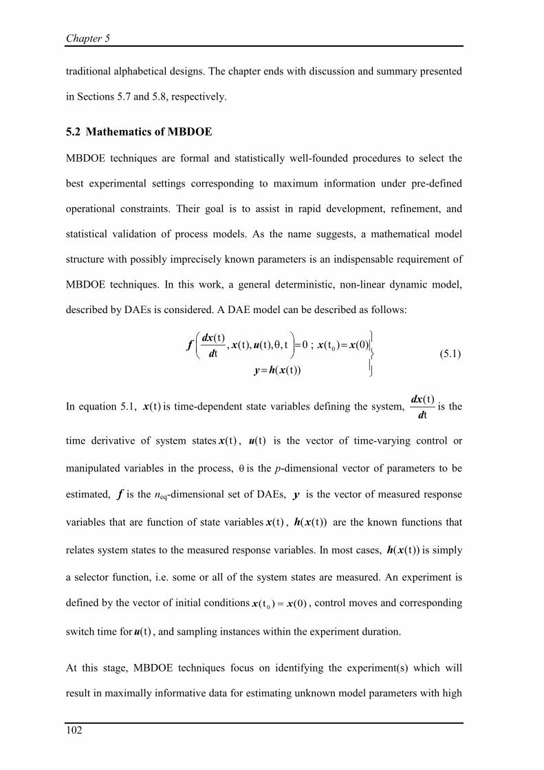
Chapter 5
102
traditional alphabetical designs. The chapter ends with discussion and summary presented
in Sections 5.7 and 5.8, respectively.
5.2 Mathematics of MBDOE
MBDOE techniques are formal and statistically well-founded procedures to select the
best experimental settings corresponding to maximum information under pre-defined
operational constraints. Their goal is to assist in rapid development, refinement, and
statistical validation of process models. As the name suggests, a mathematical model
structure with possibly imprecisely known parameters is an indispensable requirement of
MBDOE techniques. In this work, a general deterministic, non-linear dynamic model,
described by DAEs is considered. A DAE model can be described as follows:
0(t) , (t), (t), , t 0 ; (t ) (0)t
( (t))
θ = =
=
dx x u x xd
y h x
f (5.1)
In equation 5.1, (t)x is time-dependent state variables defining the system, (t)t
dxd
is the
time derivative of system states (t)x , (t)u is the vector of time-varying control or
manipulated variables in the process, θ is the p-dimensional vector of parameters to be
estimated, f is the neq-dimensional set of DAEs, y is the vector of measured response
variables that are function of state variables (t)x , ( (t))h x are the known functions that
relates system states to the measured response variables. In most cases, ( (t))h x is simply
a selector function, i.e. some or all of the system states are measured. An experiment is
defined by the vector of initial conditions 0(t ) (0)=x x , control moves and corresponding
switch time for (t)u , and sampling instances within the experiment duration.
At this stage, MBDOE techniques focus on identifying the experiment(s) which will
result in maximally informative data for estimating unknown model parameters with high

MOO based DOE
103
degree of precision. Hence, before collecting the data, based on the current mathematical
description of the process, in silico experiment(s) is/are designed, where the objective is
to adjust the available manipulated inputs so as to minimize the effect of errors on
estimated values of parameters, i.e. to make the output as ‘sensitive’ as possible to the
parameters. Data collected from the implementation of such optimal experiment(s) is used
for parameter estimation of process model under consideration. Factors such as the initial
condition for various states in the process, the experiment duration, sampling instances,
how and when the system should be perturbed, which manipulated variable(s) should be
perturbed, the best sensor locations, etc. can be the decision variables that are decided
based on the optimal solution of experimental design problem. All the decision variables
are collected in a design vector ϕ, subjected to equality or inequality constraints defining
the pre-specified operational restrictions in mathematical form. Each decision variable is
bounded between the pre-set lower and upper bounds, constituting the design space (Φ).
In addition to the operational constraints, an experiment may also involve system
constraints which must be satisfied whilst designing the optimal experiment.
Characteristically, given the initial model structure and initial guess for its parameters, the
aim of the classical DOE approaches is to minimize the parameter variance or minimize
the parameter confidence interval i.e. to make the elements of parameter variance-
covariance matrix small. A typical experiment design thus involves minimizing a metric
of variance-covariance matrix (V), or maximizing that of its inverse, the Fisher
Information Matrix (FIM). Mathematically,
( ) ( )V FIMmin arg max arg∆ = ≡ (5.2)
The FIM is (p×p) symmetric matrix and is defined as,
y y
Tij i j 0
i 1 j 1
ˆFIM( , ) G G FIM= =
θ φ = σ +∑∑n n
(5.3)

Chapter 5
104
where ijσ is the (i,j)th element of inverse of variance-covariance matrix of experimental
measurements, yn is the number of measured states (outputs), 0FIM is prior FIM from
previous experiment(s), (used in sequential experiment design). Gi is s×p matrix of first
order sensitivity coefficients at ith measured state at spn sampling instances,
isi sp
k
yG ; s 1,2,..., ;k 1,2,...,n p ∂
= = = ∂θ (5.4)
Various real-valued functions are used to quantify the FIM or variance-covariance matrix
into a scalar metric. All of them essentially focus on the eigenvalue(s) of FIM. The most
common criteria include:
1. D-optimality criterion maximizes the determinant (product of eigenvalues) of FIM,
or equivalently, minimizes the determinant of the variance-covariance matrix.
2. A-optimality criterion maximizes the trace (sum of eigenvalues) of FIM, or
equivalently, minimizes the trace of variance-covariance matrix.
3. E-optimality criterion aims to maximize the smallest eigenvalue of FIM, or
equivalently, minimizes the largest eigenvalue of variance-covariance matrix.
The geometrical interpretation of these criteria is provided in Figure 5.2. A distinct
interpretation is that A- and D-optimal designs minimize the arithmetic and geometric
mean of the identification errors, respectively, whereas the E-optimal design minimizes
the largest error [146].

MOO based DOE
105
Figure 5.2: Geometrical interpretation of the D-, A-, and E-optimal design for two parameters
Though FIM based criteria are frequently discussed in the literature, their inherent
limitations are also known. FIM is based on local first-order approximation, obtained
from the Taylor series approximation of expectation function [140], and thus apply only
approximately to non-linear systems and may not be applicable for highly non-linear
systems [151]. Notwithstanding this, only the joint confidence region based on linear
approximation of FIM is considered here, as is the common practice in MBDOE literature
[135, 140, 141, 144]. Alternatively, other approaches like bootstrap, jackknife, or Monte
Carlo simulations can be employed to characterize the uncertainty in estimated
parameters, but with associated high computational costs [152].
5.3 Parameter correlation
As mentioned earlier, the purpose of MBDOE approaches is to devise the intelligent
experiments such that the parameters estimates from the resulting experimental data are
of improved statistical quality, measured in terms of precision and de-correlation of
estimated parameters [139]. Traditional designs aim at maximizing the information
content in experimental data, resulting in improved precision of parameter estimates,
which is usually judged by a t-test [151]. However, the statistical quality of parameter
estimates cannot be decided by precision measure alone; correlation among different
model parameters should also be taken into consideration, as high parameter correlation
θ1
θ2
D Minimizes the volume of confidence
ellipse
A Minimizes the dimension of
surrounding geometry
E Minimizes the length of major axis

Chapter 5
106
afflicts the inverse problem of parameter identification [140, 145]. Interestingly, the
conventional objective of increasing the information measure alone inadvertently
increases the parameter correlation [144, 147]. Correlation among parameters can
potentially lead to convergence problems while estimating parameters [146]. Owing to
the correlation, change in one parameter can be offset by the change in other(s), leading
to the situation where various parameter combinations result in comparable values of the
objective function [146, 152, 153]. This poses problems for optimization algorithms
because no definite direction can be found in which the objective function value will
improve, leading to premature convergence of the optimization algorithm [146]. This
makes the unique identification of model parameters difficult, or even leads to inaccurate
estimates of parameters [138]. Correlation can reduce parameter precision despite good
experimental design and/or increased number of samples [147].
Correlation in parameters can manifest due to model structure (structural identifiability
issue) and/or due to noisy/sparse experimental data (practical identifiability issue) [152].
A model is structurally identifiable when under the condition of noise-free infinite
observations, one is able to uniquely identify the model parameters; otherwise, the model
is structurally unidentifiable. Existing solutions to overcome the structural unidenfiability
or structural correlation are model re-parameterization [147], parameter separation [154],
or redefining the model structure. Structural identifiability of a model does not guarantee
the unique identification of model parameters using real experimental data. The
identifiability issue owing to experimental data is addressed under practical
identifiability, which enables evaluation of the possibility of finding unique values of
parameters from the available experimental data. Here, the application of MBDOE
techniques can be very useful. Both identifiability aspects can be understood from the
simple algebraic models (equation 5.5).

MOO based DOE
107
( )2
1 1 2
x2 1
y x
y 1 e k
k k
k −
=
= − (5.5)
In the first model, estimation of the parameter combination i.e. 1 2k k is possible from
suitable experimental data, but individual estimation of 1k and 2k is impossible even
with infinite samples. Hence, the model is structurally unidentifiable. On the other hand,
in the second model, it seems that both the parameters can be estimated uniquely.
However, for very small ‘ 2xk ’ values, 2x21 e xk k−− ≈ and model 2 reduces to model 1,
which we know to be structurally unidentifiable. Thus, to estimate both the parameters in
model 2, samples should be collected for appropriate values of ‘x’. This renders model 2
an example where parameter correlation issues can arise owing to poor experimental data.
The issue can, however, be dealt with using intelligent experimental design. It may be
relatively easier to detect the practical/structural correlation for algebraic systems, but
such insights are difficult to obtain for dynamic systems [153].
Whilst researchers have discussed the issue of parameter correlation, only a few studies
have investigated the problem in detail and proposed solutions. The D-optimal design can
both reduce the parameter correlation and improve the parameter precision for two-
parameter systems, but the approach cannot be extended to model systems with three or
more parameters [140]. Modified E-optimal design, where the objective is to minimize
the condition number (ratio of maximum and minimum eigenvalues of the FIM), has also
been suggested for reducing parameter correlation [144]. Again, similar to the D-optimal
criterion, the method is effective for two-parameter systems only. A promising solution to
reduce the parameter correlation was proposed by Pritchard and Bacon [145], who instead
of opting for traditional maximization of a metric of FIM, explicitly considered an
objective function that minimizes a correlation measure [145],
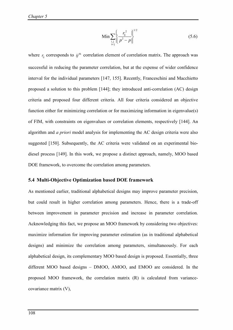
Chapter 5
108
1/22
ij2
i, ji j
Minr
p p≠
−
∑ (5.6)
where ijr corresponds to thij correlation element of correlation matrix. The approach was
successful in reducing the parameter correlation, but at the expense of wider confidence
interval for the individual parameters [147, 155]. Recently, Franceschini and Macchietto
proposed a solution to this problem [144]; they introduced anti-correlation (AC) design
criteria and proposed four different criteria. All four criteria considered an objective
function either for minimizing correlation or for maximizing information in eigenvalue(s)
of FIM, with constraints on eigenvalues or correlation elements, respectively [144]. An
algorithm and a priori model analysis for implementing the AC design criteria were also
suggested [150]. Subsequently, the AC criteria were validated on an experimental bio-
diesel process [149]. In this work, we propose a distinct approach, namely, MOO based
DOE framework, to overcome the correlation among parameters.
5.4 Multi-Objective Optimization based DOE framework
As mentioned earlier, traditional alphabetical designs may improve parameter precision,
but could result in higher correlation among parameters. Hence, there is a trade-off
between improvement in parameter precision and increase in parameter correlation.
Acknowledging this fact, we propose an MOO framework by considering two objectives:
maximize information for improving parameter estimation (as in traditional alphabetical
designs) and minimize the correlation among parameters, simultaneously. For each
alphabetical design, its complementary MOO based design is proposed. Essentially, three
different MOO based designs – DMOO, AMOO, and EMOO are considered. In the
proposed MOO framework, the correlation matrix (R) is calculated from variance-
covariance matrix (V),

MOO based DOE
109
( )
1 1 2 1 n
1 2 1 2 2 n
n 1 n 2 n
( ) ( , ) . ( , )( , ) ( ) . ( , )SSE SSEV FIM. . . .DOF DOF( , ) ( , ) . ( )
var covar covarcovar var covar
covar covar var
−
θ θ θ θ θ θ θ θ θ θ = = θ θ θ θ θ
(5.7)
ijij
ii jj
VV V
r = (5.8)
where ijV and ijr are the thij element of matrix V and R, characterizing the covariance
and correlation between thi and thj parameters, respectively. For i = j, ijV will be the
diagonal element of variance-covariance matrix and corresponds to variance of thi
parameter. SSE is the sum of squared errors between model predictions and
corresponding experimental data for obtained experimental design, and DOF corresponds
to degrees of freedom, calculated as the difference between total number of data samples
and number of estimated parameters.
The correlation matrix is symmetric with principal diagonal elements as one. The
objective function for minimizing the correlation is denoted as R . For a three parameter
system, matrix R and R are shown for illustration (equation 5.9).
12 13
2 2 221 23 12 13 23
31 32
1R 1 R
1
r rr r r r rr r
= ⇒ = + +
(5.9)
DMOO design
obj1: FIM
obj2 : R
max
min (5.10)
AMOO design
obj1: trace(FIM)obj2 : R
maxmin
(5.11)

Chapter 5
110
EMOO design
minobj1:obj2 : R
maxmin
λ (5.12)
In equation 5.12, minλ denotes the minimum eigenvalue of FIM. The second objective in
the above MOO formulations (equations 5.10 to 5.12) is one of the many possible ways
of minimizing parameter correlation. One other approach is to minimize specific
correlation elements larger than a pre-specified limit [144]. However, care should be
taken to ensure that minimizing one correlation element will not result in increasing other
correlation(s). While the MOO framework can handle more than two objectives, scope of
the present work is restricted to two objectives only.
5.5 Solution Approach (Genetic algorithm)
Non-dominated sorting genetic algorithm (NSGA-II) based solver (NGPM) available at
MATLAB Central [156], is used for solving the formulated optimization problems.
Genetic algorithm (GA) is a stochastic global optimization method that mimics the
process of natural biological evolution. It repeatedly modifies a population of individual
solutions. At each step, the GA selects individuals from the current population to be
parents and uses them to produce children for the next generation. Three main rules are
applied at each step for producing the improved population. (1) Selection rule to select
better individuals that contribute to the population at the next generation. These
individuals are also called Parents. (2) Crossover rule to combine two randomly chosen
parents to form children. (3) Mutation rule that applies random change to the children, to
form the population for the next generation. Over successive generations, the population
advances towards an optimal solution [157]. NSGA-II is an adaptation of GA for multiple
objectives. Solution of an MOO problem by this algorithm gives many equally good
optimal solutions. Set of these non-dominated solutions is also known as the Pareto-

MOO based DOE
111
optimal solutions or front [158]. Selection of an optimal point from the obtained Pareto-
optimal front depends on the desired trade-off between the conflicting objectives. In our
case, each Pareto-optimal solution corresponds to trade-off between information and
correlation measure, and an optimal experiment design.
A factor to note here is the computationally intensive nature of GA. Owing to the number
of function evaluations, the GA requires longer time to reach to the optima. For large
complex systems, the GA can be time-consuming. A simple approach to alleviate the
problem is to use a hybrid approach that combines stochastic and deterministic algorithms
[146]. Another plausible approach is to use appropriate termination criteria [158]. Since
the primary focus of this work is on the benefits of MOO in DOE, we leave out further
discussion on the computational aspects of GA.
5.6 Case Studies
To illustrate the effectiveness and applicability of the proposed MOO based DOE
framework, two case studies are considered. In both the case studies, D-, A-, E-optimal
designs, and their corresponding MOO based designs are compared. Experimental data
are simulated using true values of parameters (known a priori as this is a simulation
study) and inputs recommended by the chosen optimal experimental design. Normally
distributed random errors with pre-specified error variance-covariance matrix are added
to the simulated data to mimic, as close as possible, the characteristics of real data. The
extreme point in the Pareto-optimal front, corresponding to maximum information–
maximum correlation, belongs to alphabetical design, while the other extreme
corresponding to minimum information–minimum correlation can be considered
equivalent to Pritchard and Bacon criterion (equation 5.6). Between these two extremes,
the experimenter can select the optimal trade-off (Figure 5.3). Approaches like net flow

Chapter 5
112
method and rough set method can be employed for ranking Pareto optimal solutions and
selection [159]; however, these methods require preferences from the decision maker
(here, experimenter/modeler). Since the scope of this work is limited to illustration of
conflicting objectives in traditional DOE techniques, a relatively simple way of Pareto-
point selection is employed. In the case studies discussed, the optimal trade-off for MOO
based design and corresponding design vector are selected after transforming the obtained
Pareto-optimal front to 0 to 1 scaled Pareto-optimal front. The optimal trade-off is
selected such that the percentage decrease in information measure is less than the
percentage decrease in correlation measure. The trade-off selection is obvious when there
is significant loss in correlation measure, but little loss in information measure, e.g. see
Figure 5.8. On the other hand, for not so obvious cases, the selection is based on
eyeballing the obtained Pareto-optimal front.
Figure 5.3: Schematic representation of trade-off between information measure and correlation measure. Between the two extremes of alphabetical (D-, A-, E-) design criterion and Pritchard and Bacon criterion, experimenter has freedom to select appropriate optimal experiment design from the Pareto-optimal front. Star is one chosen design for illustration.
After implementation of the selected experiment design, model parameters are estimated
and their confidence intervals calculated. The t-value can indicate the reliable estimation
[151]:
Obj 1 – Max Information measure
Obj
2 –
Min
Cor
rela
tion
mea
sure Alphabetical
(D-, A-, E-) design
MOO based design (experimenter
decision)
Pritchard and Bacon criterion
Pareto-optimal
front

MOO based DOE
113
ii
ii
ˆ
Vt θ= (5.13)
The obtained t-value for individual parameters is tested against reference t-distribution for
n –p DOF; a t-value higher than the reference indicates that the estimate is reliable. Figure
5.4 provides a detailed flow-sheet of the approach followed here.
Figure 5.4: Schematic of the design procedure followed in the case studies
The procedure can be iterated until the obtained point estimates are close to those in the
previous iteration, and satisfy the statistical quality tests of improved precision and
Solve DAE system using θ0
Maximize information measure and minimize correlation measure
Obtain Pareto-optimal front
Select the design vector (dvec) (experimental
conditions)
Good initial guess for parameters (θ0)
Selected model structure
Design of experiments
Parameter estimation (θ)
Statistical measure (t-test, correlation)
Generate plant data using chosen dvec
Point estimates, parameter confidence
interval, and correlation
Satisfactory?
No
Final model for application(s)
Yes
Update parameter guess: θ0 = θ

Chapter 5
114
reduced correlation. Next, the case studies with their brief description, model equations,
and corresponding results are presented. In both the case studies, the manipulated variable
trajectory is parameterized as piecewise constant elements. The adopted piecewise
constant trajectory has been found to give best experimental results, and also preferred
from the operational point of view because it is easier to implement in practice [157].
5.6.1 Modified Bergman minimal model for Type 1 diabetes subjects
A model describing glucose-insulin kinetics in Type 1 diabetics is considered. Diabetes, a
disease of endocrine malfunction, is one of the most prevalent lifestyle diseases resulting
in significantly increased mortality and morbidities. A diabetic subject is either non-
responsive to insulin secreted by the pancreatic cells or the insulin secretion is
insufficient. Insulin deficient subjects are considered as Type 1 diabetes patients, and they
depend on exogenous insulin infusion for maintaining the blood glucose at acceptable
levels. In such patients, an optimal insulin infusion is required to maintain the glucose
level within permissible limits. This can be obtained by employing an appropriate
mathematical model that mimics the glucose-insulin dynamics in Type 1 diabetes patients
[160]. In this work, the modified Bergman minimal model having three parameters is
considered [161]. The model, earlier used in backoff based MBDOE [162], is given by
the following set of ODEs:
1 bG
2 3
bI
d (t)( )dtddtd (t)( )dt
G DG X G GV
X X I
I un I IV
θ
θ θ
= − − + +
= − +
= − + +
(5.14)
Here, G, X, and I represent the serum glucose concentration (mg/dL), the insulin
concentration in non-accessible compartment (mU/L), and the serum insulin

MOO based DOE
115
concentration (mU/L) above their basal values, respectively. Basal glucose concentration
(Gb = 81 mg/dL), basal insulin concentration (Ib = 15 mU/L), insulin distribution volume
(VI = 12 L), glucose distribution volume (VG = 16 L), and disappearance rate of insulin (n
= 5/54 min-1) are constant parameters in the model; and u(t) is the rate of infusion of
exogenous insulin (mU/min). The unknown model parameters are 1θ , 2θ and 3θ . In
equation 5.14, D(t) denotes meal absorption dynamics described by the following
equation [163]:
max
2max
t
A t e(t)t
tfD
−
= (5.15)
where 'A' is the amount of carbohydrates (CHO) in the meal (fixed at 75 g in this study),
max 40mint = is the time required to reach the maximum glucose concentration in the
accessible compartment, f is the dimensionless factor which represents the fraction of
CHO being absorbed (here, f = 0.8). The meal model suggests that ingested meal does not
alter the glucose concentration immediately; rather, there is a lag between food ingestion
and subsequent manifestation of glucose concentration in the blood serum.
The exogenous insulin infusion, u(t), is expressed as:
bolus basal(t)u u u= + (5.16)
Here, bolusu represents the subcutaneous bolus insulin kinetics for a bolus Ub (see equation
5.17), given at the start of experiment (at t = 0). This subcutaneous insulin dose
compensates for CHO ingestion in a "feed-forward" manner. In this in silico experiment,
the time of CHO intake is decided by the experimenter, and it can vary between 2 to 30
min after the bolus insulin dose [164]. The bolusu kinetics is given by [165]:
s 1 s
50 bbolus s s 2
50
t sT U(T t )
u−
=+
(5.17)

Chapter 5
116
where 50T is the time required to reach 50% absorption of the bolus insulin. 50T is given
by,
50 bT aU b= + (5.18)
In equations 5.17 and 5.18, the parameters a, b, and s depend on insulin type. For
Humalog insulin, a, b, and s are 5.2 min/U, 41 min, and 1.6, respectively [166].
In equation 5.16, basalu is time varying basal insulin infusion, approximated by a piecewise
constant profile. The proposed clinical test is an adaptation of oral glucose tolerance test
(OGTT), which is routinely conducted in clinical settings for measuing the glucose-
insulin sensitivity of Type 1 diabetes subjects. In OGTT, following the measurement of
fasting glucose concentration, the patient ingests 75g of CHO. Subsequently, glucose
measurements at 60 min and 120 min are taken. This test is not informative enough to
give data for estimation of unknown model parameters. Hence, a modified OGTT is
proposed here, which is similar to the one proposed by Galvanin et al. [162], with the
only difference being that the experimental duration is restricted to a maximum of 300
min. Also, only five piecewise constant moves are assumed for basal insulin infusion.
The experimental design objective is to suggest optimal basal insulin infusion profile,
amount of bolus dose at t = 0, time of meal ingestion, and corresponding blood glucose
measurement instances which will result in information-rich data for precise estimation of
θ1, θ2, and θ3, while ensuring that the correlation among estimated parameters is as low as
possible. The experiment duration is decided based on the last sampling instance. Table
5.1 lists all the design variables with their lower and upper bounds, and initial guess.

MOO based DOE
117
Table 5.1: Design variables, their bounds, and initial guess for the proposed clinical test for Type 1 diabetes subjects
Design Variable Symbol Lower Bound
Upper bound
Initial guess
Bolus insulin dose (mU) bU 0 10000 1000
CHO ingestion time At 2 30 5
Basal insulin (mU/min) basalu 16.67 300 [200, 100, 200, 0, 150]
Switch time for basalu s1t 10 300 [20, 10, 30, 25]
Sampling instances (min) tsp 10 300 [20, 50, 70, 80, 95, 115, 140, 150, 162]
The lower bound for exogenous basal insulin is fixed at 16.67 mU/min such that the
blood glucose concentration is maintained at its basal value (81 mg/dL). Several
operational constraints considered in this work are mentioned below.
1. A total of 10 blood samples (including sample at t = 0) are taken for measuring
glucose concentration [167].
2. Consecutive blood samples should have a minimum time interval of 10 min. The
maximum allowed time interval between consecutive samples is 300 min, which is
also the maximum allowed experiment duration. The last sampling instance
decides the duration of clinical test.
3. Minimum 10 min interval is mandated between two consecutive switches of basal
insulin infusion rates. Similar to the sampling constraints, the maximum switching
time is also constrained to be within 300 min.
The proposed experimental design results in 20 decision variables and 22 linear
constraints besides the model equations and physiological constraints, resulting in a fairly
challenging optimization problem – a frequent situation for generic MBDOE
implementation [141]. An intuitive approach of reducing the number of constraints is
followed here – instead of considering the switching time instant or sampling instant as

Chapter 5
118
design variables, we considered time intervals as design variables, each bounded in [10,
300]. This reduced the number of linear constraints from 22 in original optimization
problem to just 2 in the modified optimization problem. Both optimization problems are
essentially equivalent, but the latter is computationally more tractable than the original.
The modification is schematically shown for basal insulin in Figure 5.5. Similar
transformation is realized for sampling time instants.
Figure 5.5: Transformation of exact time-instants into delta-time instants
The transformation of constraints into bounds is illustrated in Table 5.2. The 22
constraints in the original formulation are transformed into 2 constraints in the modified
formulation. The switching constraint for last control move (ui5 in Figure 5.5B) is
considered to ensure that it stays for at least 10 minutes (lower bound for each control
move) within the experimental duration.
ui
ui1
ui2
ui3
ui4
ui5
t1 t2 t3 t4 T
(A)
ui
ui1
ui2
ui3
ui4
ui5
∆t1 ∆t2 ∆t3 ∆t4 T
Upper bound
Lower bound
(B)

MOO based DOE
119
Table 5.2: Transformation of constraints into bounds
(A) Original Formulation
Switching constraints
j i
j i
10; i 1, 2,3; j i 1
300
6
t tt t
constraints
− ≥= = +
− ≤
Sampling constraints
m n
m n
10; n 1,2,...,8;m n 1
30016
t tt t
constraints
− ≥= = +
− ≤
Experiment
duration
bound
end 300t ≤
(B) Modified Formulation
Switching bounds
i10 300;i 1, 2,3, 4t≤ ∆ ≤ =
Sampling bounds
j10 300; j 1, 2,...9t≤ ∆ ≤ =
Switching constraint
for last control move 9 4
j ij 1 i 1
10t t= =
∆ − ∆ ≥∑ ∑
Duration
constraint 9
jj 1
300t=
∆ ≤∑
The problem of designing the clinical test is further complicated due to additional
physiological constraints. The function of insulin is to maintain the glucose concentration
within the window of 60-120 mg/dL. However, in diabetic patients, the upper limit is
relaxed to a value such as 160 mg/dL [168]. Patients are categorized as having
experienced a hyperglycemic episode if they exceed 160 mg/dL glucose limit; in a similar
fashion, a hypoglycemic episode is said to occur when the patient’s blood glucose
concentration goes below 60 mg/dL [168]. Hypoglycemia is more dangerous than
hyperglycemia because it can result in coma or even death, thus the lower limit of 60
mg/dL may be considered as hard constraint and the upper limit of 160 mg/dL may be
regarded as soft constraint. However, for simplicity, both are considered as hard
constraints in the present simulation study. These physiological constraints are handled
using penalty function method [158]. In this approach, first the constraints are scaled and
constraint violation pertaining to hypo- and hyperglycemia for each experimental design
is calculated. The total violation is multiplied with a large weight and then added to each
objective. The penalty weight is decided based on the objective function value for
experimental design corresponding to the initial guess in Table 5.1.

Chapter 5
120
In the present simulation study, true parameters -5true = [0.025, 0.015, 1.26 10 ]θ × are used
in the patient model to generate the patient data for optimal experimental conditions. A
constant relative variance of 0.01 is added to incorporate the real-world noise
characteristics in glucose measurements. The initial parameter guess for designing the
experiment is considered at 25% positive deviation from true parameter values. They
were assumed equidistant from true parameter values so that obtained estimates and their
precision characteristics cannot be attributed to better/worse initial guess [144]. Note that,
the resulting experiment when implemented on real subjects can still violate the
permissible glucose limits due to patient-model mismatch. To prevent such undesirable
events, a conservative design approach has been considered in this work where the hypo-
and hyperglycemia limits are set at 65 and 150 mg/dL, respectively. This conservative
design may result in less information because functional value space is constrained;
however, computationally intensive robust experimental design methods such as expected
value criterion, min-max optimization [148] or backoff based technique for experiment
design [162], can overcome this problem. The robust experimental design criteria can be
incorporated in the proposed MOO based DOE framework, and will be explored in our
future work.
Traditional vs. MOO based DOE: In the simulations below, the alphabetical design (D-,
A-, and E-) and corresponding MOO based design are compared. The results for
alphabetical design typically correspond to the extreme Pareto-optimal point for
maximum information–maximum correlation, while MOO based design refers to a
chosen experimental design from the obtained Pareto-optimal front. First, the comparison
of D-optimal and DMOO design is presented – the Pareto-optimal front for DMOO based
design (Figure 5.6), the schematic of D-optimal design and the chosen DMOO based
experimental design (Figure 5.7), followed by the parameter estimates for both the

MOO based DOE
121
designs (Table 5.3). Similar sequence is followed for comparing simulation results for A-
optimal vs. AMOO design and E-optimal vs. EMOO design. In the Pareto-optimal fronts
for DMOO, AMOO, and EMOO designs (Figure 5.6, 5.8, and 5.10), the data-tip (X,Y)
corresponds to the selected optimal trade-off for implementation.
Note that FIM is based on sensitivity coefficient (equation 5.4), which is dependent on
initial guesses of parameters. The sensitivity coefficients based FIM may provide
misleading experimental design due to order of magnitude difference in model
parameters; hence, parameter-scaled sensitivity is considered for FIM calculation [169].
The parameter-scaled sensitivity ( i,G θ ) is defined as:
isi, j
j
G y θθθ
∂=∂
(5.19)
In equation 5.19, i, j, and s are the indices of measured state (Glucose), parameters (j = 1,
2, 3), and sampling instances (s = 1, 2, 3…, 10), respectively.
Figure 5.6: Pareto-optimal front for DMOO design
0 1x10¹⁶ 2x10¹⁶ 3x10¹⁶ 4x10¹⁶ 5x10¹⁶ 6x10¹⁶
0.5
0.6
0.7
0.8
0.9
1.0
1.1
1.2
X: 4.73x10¹⁶
Y: 1.005
Obj
2 -
Min
Cor
rela
tion
mea
sure
Obj1 - Max information measure
DMOO Pareto
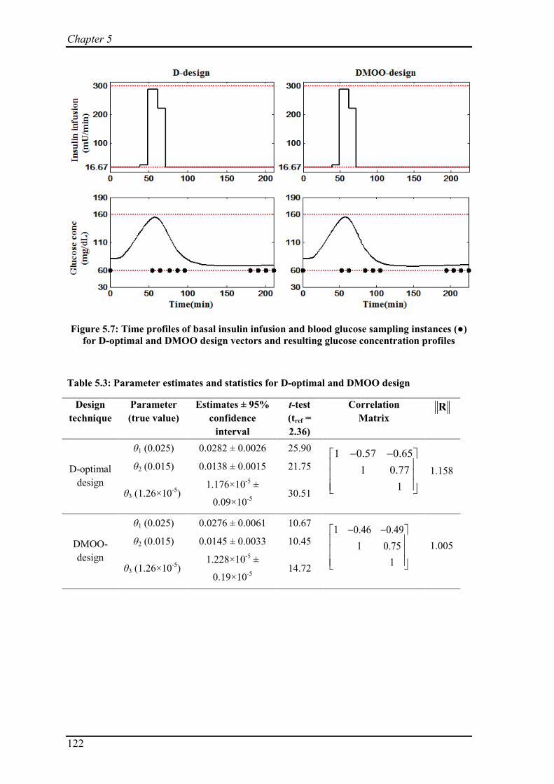
Chapter 5
122
Figure 5.7: Time profiles of basal insulin infusion and blood glucose sampling instances (●) for D-optimal and DMOO design vectors and resulting glucose concentration profiles
Table 5.3: Parameter estimates and statistics for D-optimal and DMOO design
Design technique
Parameter (true value)
Estimates ± 95% confidence
interval
t-test (tref = 2.36)
Correlation Matrix
R
D-optimal design
θ1 (0.025) 0.0282 ± 0.0026 25.90 1 0.57 0.651 0.77
1
− −
1.158 θ2 (0.015) 0.0138 ± 0.0015 21.75
θ3 (1.26×10⁻⁵) 1.176×10⁻⁵ ±
0.09×10⁻⁵ 30.51
DMOO- design
θ1 (0.025) 0.0276 ± 0.0061 10.67 1 0.46 0.491 0.75
1
− −
1.005 θ2 (0.015) 0.0145 ± 0.0033 10.45
θ3 (1.26×10⁻⁵) 1.228×10⁻⁵ ±
0.19×10⁻⁵ 14.72

MOO based DOE
123
Figure 5.8: Pareto-optimal front for AMOO design
Figure 5.9: Time profiles of basal insulin infusion and blood glucose sampling instances (●) for A-optimal and AMOO design vectors and resulting glucose concentration profiles
0.5x10⁶ 1.0x10⁶ 1.5x10⁶ 2.0x10⁶ 2.5x10⁶ 3.0x1060.4
0.6
0.8
1.0
1.2
1.4
1.6
1.8
Obj
2 -
Min
cor
rela
tion
mea
sure
Obj 1 - Max information measure
AMOO Pareto
X: 2.65x10⁶
Y: 0.862

Chapter 5
124
Table 5.4: Parameter estimates and statistics for A-optimal and AMOO design
Design technique
Parameter (true value)
Estimates ± 95% confidence
interval
t-test (tref = 2.36)
Correlation Matrix
R
A-optimal design
θ1 (0.025) 0.0770 ± 0.2371 0.77 1 0.999 0.9991 0.999
1
1.731 θ2 (0.015) 0.0185 ± 0.0164 2.67
θ3 (1.26×10⁻⁵) 1.547×10⁻⁵ ±
1.41×10⁻⁵ 2.60
AMOO- design
θ1 (0.025) 0.0254 ± 0.0164 3.66 1 0.42 0.571 0.50
1
− −
0.862 θ2 (0.015) 0.0143 ± 0.0016 21.54
θ3 (1.26×10⁻⁵) 1.218×10⁻⁵ ±
0.077×10⁻⁵ 37.27
Figure 5.10: Pareto-optimal front for EMOO design
0 2x10⁴ 4x10⁴ 6x10⁴ 8x10⁴ 10x104 12x104
0.50
0.55
0.60
0.65
0.70
0.75
Obj
2 - M
in c
orre
latio
n m
easu
re
Obj 1 - Max information measure
EMOO Pareto
X: 9.513x10⁴
Y: 0.697

MOO based DOE
125
Figure 5.11: Time profiles of basal insulin infusion and blood glucose sampling instances (●) for E-optimal and EMOO design vectors and resulting glucose concentration profiles
Table 5.5: Parameter estimates and statistics for E-optimal and EMOO design
Design technique
Parameter (true value)
Estimates ± 95% confidence
interval
t-test (tref = 2.36)
Correlation Matrix
R
E-optimal design
θ1 (0.025) 0.0263 ± 0.0043 14.41 1 0.11 0.131 0.71
1
−
0.735 θ2 (0.015) 0.0143 ± 0.0020 16.83
θ3 (1.26×10⁻⁵) 1.228×10⁻⁵ ±
0.160×10⁻⁵ 18.17
EMOO- design
θ1 (0.025) 0.0261 ± 0.0047 13.11 1 0.10 0.121 0.68
1
−
0.697 θ2 (0.015) 0.0151 ± 0.0022 15.94
θ3 (1.26×10⁻⁵) 1.220×10⁻⁵ ±
0.169×10⁻⁵ 17.03
From the results in Tables 5.3 to 5.5, it can be observed that each MOO based
experimental design performs better or equivalent to its alphabetical counterpart. For D
vs. DMOO and E vs. EMOO scenarios, the decrease in correlation comes at a small cost
of decreased parameter precision, but they give improved point estimates, which are

Chapter 5
126
closer to true values of parameters. Both D-optimal and DMOO-designs result in similar
basal insulin profiles, however, a closer inspection will indicate that the DMOO-design
results in slightly longer experiment duration and different sampling instances (Figure
5.7). A-optimal design results in significantly high correlation among parameters, with all
correlation elements close to 1. This results in poor point estimates as well as smaller t-
value for parameters (Table 5.4). It is clear from Figure 5.8 that the selected AMOO
experimental design provides a precipitous decrease in correlation measure with little loss
in information measure. The resulting point estimates for individual parameters are closer
to true values with significantly high t-values (Table 5.4).
The proximity of obtained parameter estimates is compared based on percentage
normalized Euclidean distance (δ) between obtained parameter estimates and true
parameters.
2
ni,true i
i 1 i,true
100 ; n number of parametersθ θθ=
−δ = × =
∑ (5.20)
The results are summarized in Table 5.6. In all three scenarios, the percentage normalized
Euclidean distance is smaller for MOO based designs, which confirms that the resulting
parameter estimates from MOO based designs are closer to the true values of model
parameters when compared with the corresponding alphabetical designs.
Table 5.6: Percentage normalized Euclidean distance for alphabetical and MOO based designs for Type 1 diabetes model
Alphabetical vs. MOO design δtraditional δMOO
D vs. DMOO 16.62 11.12
A vs. AMOO 210.59 5.83
E vs. EMOO 7.29 5.57

MOO based DOE
127
5.6.2 Baker’s Yeast Fermentation Reactor Model
This case study corresponds to fed-batch model for Baker’s yeast fermentation [170].
This classical model has been widely employed for implementation of various DOE
techniques such as D-optimal [171], E-optimal [142], SV-optimal [142], min-max robust
optimal [148], P-optimal [141], and anti-correlation experimental design [150], and can
be considered as a benchmark model in MBDOE literature. Assuming Monod kinetics for
substrate consumption and biomass growth, the reactor model can be described by the
following set of DAEs:
11 4 1
2 11 2 2
3
1 2
2 2
( ).
. ( )
dy r u ydt
dy r y u u ydt
yry
θ
θ
θθ
= − −
= − + −
=+
(5.21)
where 1y and 2y are the biomass and substrate concentrations (g/L), respectively and r is
the specific growth rate of bio-mass. The reactor system uses two piecewise constant
manipulated variables 1u (dilution factor, h-1) and 2u (feed substrate concentration, g/L).
The reactor model has four unknown parameters, of which two are for the rate expression
( 1θ , 2θ ) and the rest two are yield coefficients ( 3θ , 4θ ). At t = 0, the substrate
concentration 02y equals 0.1 and biomass concentration denoted by 0
1y is a design
variable, i.e. 00 1[ ,0.1]y y=
The design variables comprise 01y , five manipulated variable moves for each of 1u and 2u ,
four switching times for each manipulated variable, and ten sampling instances. In effect,
the design space constitutes a total of 29 decision variables. All the design variables with
their lower and upper bounds, and initial guess values are summarized in Table 5.7.

Chapter 5
128
Table 5.7: Design variables, their bounds, and initial guess values for Baker's yeast fermentation reactor system
Design Variable Symbol Lower Bound
Upper bound
Initial guess
Initial amount of Biomass 01y 1 10 5.5
Sampling instances (h) spt 0.5 20 [2, 6, 9, 16, 21, 23, 27, 33, 36, 38]
Dilution factor (L-1) 1u 0.05 0.2 [0.12, 0.12, 0.12, 0.12, 0.12]
Substrate in feed (g L-1) 2u 5 35 [15, 15, 15, 15, 15]
Switch time for 1u s1t 0.5 20 [5, 15, 20, 30]
Switch time for 2u s2t 0.5 20 [5, 15, 20, 30]
The operational constraints considered in the design are as follows:
• Minimum and maximum duration between consecutive control switches is 0.5 and
20 hours, respectively.
• Two consecutive samples should be at least 0.5 hours apart and at most 20 hours
apart [141].
• The first sample could only be taken after 0.5 hours of start of experiment.
• Maximum allowable experiment duration is 40 hours.
Based on the above constraints, a total of 30 linear constraints were obtained for
experimental design, besides the model equations. These were reduced to 3 by employing
the earlier mentioned approach of transforming the time instants to time intervals (Figure
5.5 and Table 5.2), each bounded between [0.5, 20]. Corresponding to measured states,
1y and 2y , the error variance matrix ∑ is assumed to be diagonal and following a constant
relative variance model [141]:
0.04 0
0 0.04
=
∑ (5.22)

MOO based DOE
129
The true parameter values for this system were, θtrue = [0.31, 0.18, 0.55, 0.05]. These
values were used to obtain the "experimental data" from the model. For all the
experimental designs, the initial parameter guess, θ = [0.5, 0.5, 0.5, 0.5] is used. In the
parameter estimation stage, following upper and lower bounds on parameters were
imposed [141]:
1 2 3 40.05 , , 0.98 0.01 0.98< < < <θ θ θ θ (5.23)
Traditional vs. MOO based DOE
i,G yθ
: Similar to the first case study, comparison of parameter
estimates, correlation, and t-value for D-, A-, and E-optimal design with their respective
MOO counterparts are tabulated in Tables 5.8, 5.9, and 5.10, respectively. Figures 5.12,
5.14, and 5.16 are Pareto-optimal fronts corresponding to DMOO, AMOO, and EMOO
design, respectively; in these figures, the data-tip (X,Y) corresponds to the selected
optimal trade-off for implementation. As in the first case study, parametric scaling of
sensitivity coefficients is adopted. In addition, the sensitivity coefficients are also scaled
with respect to states in order to remove the magnitude difference between different
measured states. The modified scaled sensitivity is defined as response-ranged sensitivity
( ) [169]:
jisi,
j i,max i,min
G y θyθ y yθ
∂=∂ −
(5.24)
In this equation, ‘i’ is the index of measured state (both states 1y and 2y are measured),
‘s’ is the index for sampling instance (s = 1, 2,…,10), and ‘j’ is the index for parameters (j
= 1, 2, 3, 4).
Figures 5.13, 5.15, and 5.17 show the optimal time profiles for dilution factor ( 1u ) and
substrate in feed ( 2u ); all these figures show profiles for traditional designs and their

Chapter 5
130
MOO design counterpart along with sampling instances, and the dotted lines in the
figures denote the lower and upper bounds for manipulated variables 1u and 2u .
Figure 5.12: Pareto-optimal front for DMOO design
Figure 5.13: Time-profile of manipulated vairables ( 1u and 2u ) and sampling instances (●) for D-optimal and DMOO design
0.0 0.5x10⁹ 1.0x10⁹ 1.5x10⁹ 2.0x10⁹
0.8
1.0
1.2
1.4
1.6
1.8
2.0
Obj
2 :
Min
cor
rela
tion
mea
sure
Obj 1 : Max information measure
DMOO Pareto
X: 1.6x10⁹
Y: 1.93
0 2 4 6 8 10 12
0.05
0.1
0.15
0.2
u 1 (Dilu
tion
fact
or)
D-design
0 2 4 6 8 10 12 13.7
5
15
25
35
u 2 (Fee
d su
bstr
ate
conc
entr
atio
n)
Time (hr)
0 2 4 6 8 10 12 13.3
0.05
0.1
0.15
0.2
DMOO-design
0 2 4 6 8 10 12 13.3
5
15
25
35
Time (hr)

MOO based DOE
131
Table 5.8: Parameter estimates and statistics for D-optimal design and DMOO design
Design technique
Parameter (true value)
Estimates ± 95% confidence
interval
t-test (tref = 2.12)
Correlation Matrix
R
D-optimal design
θ1 (0.31) 0.275 ± 0.632 0.92* 1 0.60 0.95 0.9971 0.64 0.64
1 0.941
− − −
1.986 θ2 (0.18) 0.242 ± 1.031 0.50* θ3 (0.55) 0.602 ± 0.199 6.42 θ4 (0.05)
0.061 ± 0.030 4.34
DMOO- design
θ1 (0.31) 0.407 ± 0.419 0.94* 1 0.54 0.94 0.9971 0.61 0.58
1 0.931
− − −
1.933 θ2 (0.18) 0.222 ± 0.415 0.69* θ3 (0.55) 0.537 ± 0.193 5.14 θ4 (0.05)
0.049 ± 0.025 3.39
* Statistically insignificant parameter(s)
Figure 5.14: Pareto-optimal front for AMOO design
0.0 0.5x10⁵ 1.0x10⁵ 1.5x10⁵ 2.0x10⁵ 2.5x10⁵ 3.0x10⁵
0.8
1.0
1.2
1.4
1.6
1.8
2.0
2.2
Obj
2 -
Min
cor
rela
tion
mea
sure
Obj 1 - Max information measure
AMOO Pareto
X: 2.415x10⁵
Y: 1.66

Chapter 5
132
Figure 5.15: Time-profile of manipulated vairables ( 1u and 2u ) and sampling instances (●) for A-optimal and AMOO design.
Table 5.9: Parameter estimates and statistics for A-optimal design and AMOO design
Design technique
Parameter (true value)
Estimates ± 95% confidence
interval
t-test (tref = 2.12)
Correlation Matrix
R
A-optimal design
θ1 (0.31) 0.389 ± 0.152 5.42 1 0.69 0.99 0.9991 0.73 0.71
1 0.991
− − −
2.113 θ2 (0.18) 0.310 ± 0.246 2.66 θ3 (0.55) 0.570 ± 0.203 5.95 θ4 (0.05)
0.053 ± 0.023 4.92
AMOO- design
θ1 (0.31) 0.315 ± 0.176 3.80 1 0.12 0.94 0.9931 0.04 0.23
1 0.901
− −
1.660 θ2 (0.18) 0.210 ± 0.189 2.35 θ3 (0.55) 0.620 ± 0.256 5.14 θ4 (0.05)
0.060 ± 0.027 4.68
0 5 10 15 20
0.05
0.1
0.15
0.2
u 1 (
Dil
utio
n fa
ctor
)A-design
0 5 10 15 20
5
15
25
35
u 2 (Fee
d su
bstr
ate
conc
entr
atio
n)
Time (hr)
0 5 10 15 20
0.05
0.1
0.15
0.2
AMOO-design
0 5 10 15 20
5
15
25
35
Time (hr)

MOO based DOE
133
Figure 5.16: Pareto-optimal front for EMOO design
Figure 5.17: Time-profile of manipulated vairables ( 1u and 2u ) and sampling instances (●) for E-optimal and EMOO design.
0 1 2 3 4 5 60.85
0.90
0.95
1.00
1.05
1.10
Obj
2 -
Min
corre
latio
n m
easu
re
Obj 1 - Max information measure
EMOO Pareto
X: 5.069Y: 1.004
0 5 10 15 20
0.05
0.1
0.15
0.2
u 1 (Dilu
tion
fact
or)
E-design
0 5 10 15 20
5
15
25
35
u 2 (Fee
d su
bstr
ate
conc
entr
atio
n)
Time (hr)0 5 10 15 20
5
15
25
35
Time (hr)
0 5 10 15 20
0.05
0.1
0.15
0.2
EMOO-design

Chapter 5
134
Table 5.10: Parameter estimates and statistics for E-optimal design and EMOO design
Design technique
Parameter (true value)
Estimates ± 95% confidence
interval
t-test (tref = 2.12)
Correlation Matrix
R
E-optimal design
θ1 (0.31) 0.230 ± 0.117 4.17 1 0.09 0.31 0.971 0.25 0.11
1 0.271
− −
1.095 θ2 (0.18) 0.176 ± 0.203 1.84* θ3 (0.55) 0.483 ± 0.131 7.84 θ4 (0.05)
0.042 ± 0.016 5.46
EMOO- design
θ1 (0.31) 0.275 ± 0.167 3.49 1 0.08 0.18 0.971 0.06 0.14
1 0.081
− −
1.004 θ2 (0.18) 0.173 ± 0.177 2.08* θ3 (0.55) 0.547 ± 0.172 6.75 θ4 (0.05)
0.050 ± 0.019 5.49
* Statistically insignificant parameter(s)
In all the three MOO based designs, point estimates of parameters are close to true
parameter values (Table 5.8, 5.9, and 5.10). The proximity of these to true parameter
values are compared based on percentage normalized Euclidean distance (δ), defined in
equation 5.20. The results are summarized in Tables 5.6 and 5.11. Considering D- vs.
DMOO designs, only a small decrease in correlation measure can be obtained for a
somewhat large decrease in information measure (Figure 5.12). This is reflected in
obtained parameter estimates for both designs, which are similar with two parameters
turning out to be statistically insignificant (Table 5.8). D-optimal design results in more
precise parameters, while DMOO design results in slightly better point estimates. This
suggests that based on one’s requirement, the alphabetical design or MOO based design
can be preferred. If the parameter precision is more important, then one should opt for D-
design, and if focus is on accurate point estimates then one should opt for DMOO design.
Similarly, the AMOO design outperforms A-optimal design while considering point
estimates, but result in slightly poor t-values or wider confidence interval (Table 5.9).

MOO based DOE
135
Similar results are obtained for E-EMOO pair where improved point estimates are
obtained at the cost of wider confidence interval (Table 5.10).
Table 5.11: Percentage normalized Euclidean distance for alphabetical and MOO based designs for Baker’s yeast fermentation reactor model
Alphabetical vs. MOO design δtraditional δMOO
D vs. DMOO 43.30 39.07
A vs. AMOO 76.87 28.40
E vs. EMOO 32.59 11.84
5.7 Discussion
The foremost advantage of the proposed MOO based DOE framework is that it results in
multiple optimal experiment designs in the form of a Pareto-optimal front. The two
extremes of Pareto-optimal front can be considered equivalent to single objective designs:
one extreme corresponds to maximum information–maximum correlation which is
equivalent to the traditional alphabetical design, while the other extreme refers to
minimum information–minimum correlation, equivalent to the design for Pritchard and
Bacon criterion [145]. Between these two extremes, there exist a number of optimal
trade-offs between information and correlation measures. This offers the experimenter the
freedom to choose an optimal experiment design according to the desired trade-off. From
the results on the two case studies, it can be concluded that MOO based designs result in
better point estimates than the traditional alphabetical designs. The improved point
estimates are obtained at the cost of slightly decreased precision in MOO based designs.
The decreased precision is expected owing to the fact that MOO based experimental
design opts for decreased information measure. This decreased information contributes
towards poor precision of estimated parameters. Note that the comparison of results is
based on the chosen optimal trade-off between information and correlation measure and
the respective alphabetical design.
Chapter 5
136
Interestingly, the AMOO-design results for Type 1 diabetes model clearly outperforms
those from the A-optimal design, both in the context of point estimates as well as
parameter precision (Table 5.4). Even in the Baker’s yeast fermentation reactor case
study, the A-optimal design results in poorer point estimates (Table 5.9); this is also
evident from Table 5.11, where the worst percentage normalized Euclidean distance (δ) is
obtained for A-optimal design. Earlier, it has been recommended that A-optimal criterion
should not be employed for experimental design since it may lead to non-informative
experiments due to high correlation in parameters [140]. Results of the present simulation
study show that AMOO design can overcome the problems associated with A-optimal
design and results in better parameter estimates. Among the discussed alphabetical
designs, E-optimal design performs better for the two case studies, but EMOO-design
performs even better than E-optimal design, as can be observed from percentage
normalized Euclidean distance (δ) in Tables 5.6 and 5.11. The lower value of δ indicates
that the obtained point estimates for parameters are closer to true parameter values.
Further, comparison of the obtained Pareto-optimal fronts for DMOO, AMOO, and
EMOO designs shows that the point corresponding to minimum correlation measure is
very similar in all the designs (Figures 5.6, 5.8, and 5.10 for Type 1 diabetes model, and
Figures 5.12, 5.14, and 5.16 for Baker’s yeast fermentation reactor model). The minor
discrepancy could be attributed to the stochastic nature of genetic algorithm employed.
Notably, the other extreme corresponding to maximum information–maximum
correlation i.e. alphabetical design shows the least value for EMOO Pareto-optimal front,
when compared with corresponding DMOO and AMOO Pareto-optimal fronts. This
suggests that this particular extreme point in EMOO Pareto-optimal front or E-optimal
design can also reduce parameter correlation. In other words, among the alphabetical
designs, E-optimal design can better handle the correlation among parameters.
MOO based DOE
137
Results of the case studies show that the obtained Pareto-optimal fronts for the two case
studies are different for the same design. Also, for each case study, the Pareto-optimal
front is different for different designs. This suggests that shape of the Pareto-optimal front
depends on model equations, number of parameters, and the choice of design criteria. The
other plausible factors affecting the shape of the Pareto-optimal front are number of
measured states, number of samples, and input perturbation allowed. Generally, the
correlation among parameters increases with increase in information, but the actual trade-
off needs to be established for each scenario by MOO.
5.8 Summary
An MOO based DOE framework, which provides an optimal trade-off between
information for parameter estimation and correlation among parameters, is proposed. Two
case studies, namely, a 3-parameter modified Bergman minimal model for Type 1
diabetes patients and a 4-parameter Baker’s Yeast fermentation model are used to
illustrate the effectiveness of the proposed approach. The results highlight the potential of
MOO based DOE formulations to perform better than the traditional alphabetical designs.
Specifically, the proposed approach can provide point estimates closer to the true values
than those obtained by the traditional alphabetical designs; the AMOO design overcomes
the problems associated with A-optimal design. Among the alphabetical designs, the E-
optimal design is superior in reducing the correlation among parameters, but EMOO
design performs even better.

Chapter 6
138

Optimal HD sampling
139
6. Optimal Sampling Protocol for Toxin Kinetic Modeling
If your experiment needs statistics, you ought to have done a better experiment.
- Ernest Rutherford
Part 2 of the thesis started with the premise that, if better estimates of inter-
compartmental clearance (Kip) and/or other model parameters are obtained, then exercise
induced physiological changes can be better quantified. To obtain precise estimates of the
model parameters, an intelligent experiment design is a pre-requisite. Towards this end,
the previous chapter proposed a novel MOO based DOE framework for experimental
design. The proposed DOE framework was tested on two case studies. It was shown that
though traditional MBDOE techniques maximize the information content for precise
parameter estimation, they also increase the correlation among model parameters. In this
chapter, the same framework will be used on the proposed toxin kinetic model (TKM) in
Chapter 3. The objective here is not to compare the performance of alphabetical and
MOO based DOE, but to provide the optimal sampling protocol for TKM. Hence, only D-
optimal design and its MOO based counterpart will be studied. The D-optimal design is
chosen because it is the most popular experimental design criterion [140].
6.1 Sampling protocols in TKM
To improve the existing dialysis care i.e. obtaining enhanced toxin removal, TKM can
play an important role [69]. For details of TKM and related literature, see Chapter 2
where a review of TKM has been presented. Briefly, TKM relates to the mathematical
approximation of physiology. A number of mathematical representations such as single-
pool model, two-pool model, regional blood flow model, and diffusion-adjusted regional
blood flow model are available to approximate the physiology. Irrespective of the type of
model employed, all of them have unknown model parameters whose estimation is
necessary before the model can be employed to understand the toxin kinetics and to

Chapter 6
140
decipher how the dialysis adequacy can be increased for pathophysiologically important
toxins. A better understanding of the toxin kinetic behavior not only provides a rational
for choosing dialysis dose [172], but also gives important insights about physiological
resistance responsible for inadequate toxin removal [173]. The aspects related to
physiological resistance were detailed in Chapter 3, and change in this resistance as a
result of intra-dialytic exercise was presented in Chapter 4. The physiological changes
related to inter-compartmental toxin transfer are lumped in a model parameter Kip, which
is inversely proportional to inter-compartmental resistance. The precise estimation of Kip
can not only quantify the exercise induced physiological changes, but also provide a
better estimate of toxin removal. Apart from Kip, estimation of other model parameters
can facilitate a better understanding of patient physiology [29, 173].
Parameter estimation necessitates toxin concentration measurement, and number of blood
samples are collected during and post-dialysis phase. The importance of intelligent
sampling is paramount considering the significance of TKM [69]. Numerous sampling
practices exist in the TKM literature (Table 6.1); but an important question remains
unanswered: Which sampling protocol is superior (to others)? Specifically, when and how
many samples should be collected such that precise estimates for physiologically
important model parameters can be obtained? MBDOE techniques can potentially play an
important role in this regard, because a good physiological representation in the form of
DA-RBF model already exists (Chapter 3). The MBDOE paradigm has already been
realized in engineering, systems biology domain [140], and also in biomedical fields such
as diabetes care [167]. Despite this, there is no mention or use of MBDOE in TKM
literature. This chapter intends to fill this gap.

Optimal HD sampling
141
Table 6.1: Existing sampling protocols for various uremic toxins
Reference Solute Dialysis regimen
Kinetic modeling approach
Sampling instances during dialysis
Sampling instances post-dialytic
Total samples
Eloot et al.[67] Urea, Guanidino compounds
HD Two-pool model 0, 5, 15, 30, 120, end dialysis No sample 6
Schneditz et al.[51]*
Urea, Creatinine HD DA-RBF model 0, 5, 15, 30, 120, end dialysis No sample 6
Yashiro et al.[87] Urea HD RBF model 0, 15, 30, 45, 60, 90, 120, 180, 240
60 10
Liberati et al.[174]
Urea HD Bi- and Tri-compartment model
0, 5, 10, 30, 100, 240 5, 10, 30 ,60 10
DeSoi et al.[55]**
Phosphate HD Two-pool model 0, 15, 30, 45, 60, 90, 120, 150, 180, 210, 240
15, 30, 45, 60, 90, 120, 150, 180, 210, 240
21
Spalding et al.[56]
Phosphate HD/HDF Four-pool model 0, 40, 80, 120, 160, 200, 240 2, 15, 30, 60 11
Ursino et al.[63] K+, Na+, Cl-, Urea, HCO3
-, H+ Profiled HD Two-pool model 0, 20, 40, 60, 80, 100, 120,
140, 160, 180, 200, 220, 240 No sample 13
Leypoldt et al.[72]
β2-microglobulin HD Two-pool model 0, 60, 120, 180, 210 20 sec, 2, 10, 20, 30, 60 11
Stiller et al.[73] β2-microglobulin HD Two-pool model 0, 30, 60, 120, 180, 240 10, 20, 30, 40, 50, 60 12 Ward et al.[74] β2-microglobulin HDF Two-pool model 0, 60, 120, 240 20 sec, 5, 10 ,30 ,60, 90
120, 240 12
Maheshwari et al.[173]***
β2-microglobulin HDF DA-RBF model 0, 60, 120, 240 20 sec, 5, 10 ,30 ,60, 90 120, 240
12
* Urea and creatinine concentrations reported by Eloot et al.[67] were used for the study. ** Recruited study subjects dialyzed for different durations. The sampling protocol presented here reflects 4 hour dialysis. *** β2-microglobulin concentrations reported by Ward et al.[74] were used for the study.

Chapter 6
142
As mentioned earlier, different sampling protocols exist in the context of TKM. However,
no definite consensus exists for sampling during and post-dialysis period (Table 6.1).
Also, how many samples should be collected for precise estimation of model parameters
remains an unstudied problem. Different clinical studies follow different sampling
protocols, without accounting for the fact that those sampling protocols may be expensive
due to too many samples and/or uninformative due to sampling decisions based on
intuition. The objective of this work is to provide an optimal sampling protocol for
precise estimation of DA-RBF model parameters. In the next section, experimental design
details are presented. Obtained sampling protocols and results from MBDOE paradigm
are presented in Section 6.3. A discussion on the obtained results is presented in Section
6.4. The last section summarizes the important insights developed from this investigation.
6.2 Materials and Methods
The foremost requirement for MBDOE techniques is a mathematical model with some a
priori knowledge of values for unknown model parameters. In this work, the DA-RBF
model, which arguably is the most comprehensive TKM available at present, is employed
for elucidating the optimal sampling protocol. The toxin considered is β2-microglobulin, a
marker of middle-sized uremic toxins and also an independent marker of mortality and
morbidity in maintenance HD patients [75]. The model description, equations, and related
details can be found in Chapter 3. The original model comprised seven parameters, which
were reduced to three parameters using a priori identifiability analysis (Section 3.3). The
three model parameters that need to be estimated are Kip, Vd, and fP. The measured state is
arterial serum concentration (Cart).
Toxin Kinetic Model
Optimal HD sampling
143
As mentioned in the previous chapter, central to the MBDOE techniques is the Fisher
Information Matrix (FIM) which is calculated from sensitivity coefficients. In this
particular model, the corresponding sensitivity coefficient defined at each sampling
instant (tj) is:
art , jij
i
Z ; where i 1, 2,3 jC
and sampling instance∂
= = =∂θ
(6.1)
Note that ijZ corresponds to ijth element of sensitivity coefficient matrix (Z), whose size
depends on the number of samples; e.g., if 10 samples are collected for estimating 3
parameters, then the size of Z matrix is 10×3.
The flowchart of employed MBDOE methodology is shown in a previous chapter (Figure
5.4), which starts with model selection and initialization of model parameters. The model
structure corresponds to the DA-RBF model. The initial guess for parameters can be
obtained from the literature or from an understanding of patient physiology; e.g., β2-
microglobulin distribution volume (Vd) corresponds to extracellular fluid volume which is
typically 33% of total body water. In this simulation study, the true value of patient
parameters is known and the design objective is to obtain the output samples at optimal
times that will result in point estimates closer to the true values. The true values of model
parameters were taken as the mean estimates from Chapter 3. The initial guess for Kip, Vd,
and fP were chosen at 50%, 20%, and 20% negative deviation from known true values.
The inter-compartmental clearance is considered to have a larger deviation because it
cannot be measured, while the Vd and fP can be inferred from patient physiology. The true
parameter values along with their initial guess values (for MBDOE purposes) are
presented in Table 6.2.
Experimental Design Information

Chapter 6
144
Table 6.2: Model parameters with their known true values and initial guesses used for model-based design of experiment techniques
Parameter True Value [173] Initial guess (% deviation
from true values)
Kip 44 mL/min 22 mL/min (-50%)
Vd 14 L 11.2 L (-20%)
fP 0.39 0.31 (-20%)
Two important considerations in the experimental design for TKM are the experiment
duration and the number of samples. From Table 6.1, it can be noted that different TKM
studies have followed different criteria for both these aspects. First, for the experiment
duration, it can be suggested that smaller the experiment duration the more convenient it
is for the patients; however, it cannot be less than 240 min dialysis duration and so the
decision variable with clinician/experimenter is the post-dialysis wait. In Table 6.1, the
post-dialysis ranges from 0 to 240 min. To ascertain the optimal duration of experiment,
different experiment duration (including post-dialysis wait), namely, 240 min, 300 min,
360 min, and 480 min are studied independently. The second important aspect for TKM
experiment design is the total number of samples. Again, from Table 6.1, it is clear that a
wide variety of sampling protocol exists. The important question is: should all the
samples be collected in intra-dialytic phase, or more samples should be collected during
intra-dialytic phase and less in post-dialysis phase, or vice-versa? Here, four different
scenarios for total number of samples are considered (Table 6.3). The MBDOE will
automatically decide the distribution of sampling instances in intra-dialysis phase as well
as post-dialysis phase. For each of the experiment duration, individual sampling scenario
is considered. In effect, total 16 scenarios as mentioned in Table 6.3 are considered. Note
that, in design procedure, the pre-dialysis sample (at t = 0) and end-dialysis sample (t =
240 min) are mandatory because these are conventionally required for estimation of

Optimal HD sampling
145
D ureat / VK or toxin reduction ratio. To account for this, the decision variables in Table
6.3 exclude the sample at t = 0, but sample at t = 240 is decided by MBDOE itself. If
MBDOE does not result in t = 240 min in the final sampling protocol, then sampling t =
240 is included for final parameter estimation. Few operational constraints were also
incorporated in the experimental design: a minimum gap of 5 minutes is maintained
between two consecutive samples. At the same time, maximum time interval between two
consecutive samples is restricted to 120 min.
Table 6.3: Two factors – Experiment duration and number of decision variables, each at 4 levels
Number of decision variables (dv)
Exp
erim
ent d
urat
ion
240 min 6 dv
240 min 8 dv
240 min 10 dv
240 min 12 dv
300 min 6 dv
300 min 8 dv
300 min 10 dv
300 min 12 dv
360 min 6 dv
360 min 8 dv
360 min 10 dv
360 min 12 dv
480 min 6 dv
480 min 8 dv
480 min 10 dv
480 min 12 dv
Here, the objective is to suggest the optimal sampling instances for TKM, based on D-
optimal design. At the same time, the DMOO design is also studied. In all the 16
scenarios, the arterial serum toxin concentration is obtained at these optimal sampling
instances using the model with true parameter values. To incorporate the characteristics
of real-time data, 10% relative noise was added to all the samples. In clinical setting, the
data will be obtained from actual measurement during intra- and post-dialysis. This data
is used for parameter estimation and subsequent calculation of parameter confidence
interval. The entire procedure highlighted above was repeated for all the 16 scenarios
shown in Table 6.3. In all the scenarios, it is assumed that post-dialysis fluid intake is at
constant rate (α), while there is no fluid intake during dialysis.

Chapter 6
146
6.3 Results
The MBDOE and parameter estimation procedure was repeated for each scenario. The
sampling instances for each experiment scenario are shown in Table 6.4. In Table 6.5,
only optimal sampling instances are shown. The mandatory samples at t = 0 and t = 240
min are not shown. In some scenarios, t = 240 is the sampling instance from optimizer
itself, and hence included in Table 6.5. For DMOO-design, the presented sampling
instances correspond to chosen trade-off solution from the Pareto-optimal front. For each
of the 16 scenarios, one Pareto-optimal front was obtained. For illustration, only four of
these Pareto-optimal fronts for the case of 8 decision variables, one each for experimental
duration, are presented in Figures 6.1 to 6.4. The data-tip in each of these figures
corresponds to the chosen experimental design.
Figure 6.1: Pareto-optimal front for 240 min
0 5000 10000 150000.9
0.95
1
1.05
1.1
1.15
1.2
1.25
1.3
X: 1.11e+004Y: 1.198
Obj1 - Max information
Obj
2 -
Min
cor
rela
tion
DMOO Pareto for experiment dutation 240 min
experiment duration and 8 decision variables

Optimal HD sampling
147
Figure 6.2: Pareto-optimal front for 300 min
experiment duration and 8 decision variables
Figure 6.3: Pareto-optimal front for 360 min
0 1 2 3 4x 10⁴
0.9
1
1.1
1.2
1.3
1.4
1.5
1.6
X: 2.852e+004Y: 1.432
Obj1 - Max information
Obj
2 -
Min
cor
rela
tion
DMOO Pareto for experiment duration 300 min
experiment duration and 8 decision variables
0 2 4 6 8x 10⁴
0.9
1
1.1
1.2
1.3
1.4
1.5
X: 4.646e+004Y: 1.317
Obj1 - Max information
Obj
2 -
Min
cor
rela
tion
DMOO Pareto for experiment duration 360 min

Chapter 6
148
Figure 6.4: Pareto-optimal front for 480 min
As mentioned earlier, in this simulation study, the patient model with known true
parameter values is assumed as proxy to the patient, and it is simulated to obtain the toxin
concentration at the optimal sampling instances. The obtained data was used to estimate
the unknown model parameters Kip, Vd, and fP. To evaluate the individual parameter
precision, the t-value for individual parameter is calculated. At the same time, the point
estimates were compared using percentage normalized Euclidean distance (δ) between
obtained parameter estimates and true parameters (equation 5.20). In Table 6.5, obtained
point estimates with t-value and the δ are shown for comparative analysis. Larger t-value
for individual parameter indicates improved precision while smaller value of δ denotes
superior point estimates.
experiment duration and 8 decision variables
0.5 1 1.5 2 2.5x 10⁵
0.55
0.6
0.65
0.7
0.75
0.8
0.85
0.9
0.95
1
X: 1.93e+005Y: 0.8078
Obj1 - Max information
Obj
2 -
Min
cor
rela
tion
DMOO Pareto for experiment duration 480 min

Optimal HD sampling
149
Table 6.4: Decision variables (d.v.) or optimal sampling instances in different experiment duration (during dialysis + post-dialysis). Sampling instances during dialysis (normal text) and post-dialysis (bold text), respectively.
240 min 300 min 360 min 480 min 6 d.v. 8 d.v. 10 d.v. 12 d.v. 6 d.v. 8 d.v. 10 d.v. 12 d.v. 6 d.v. 8 d.v. 10 d.v. 12 d.v. 6 d.v. 8 d.v. 10 d.v. 12 d.v.
D-o
ptim
al d
esig
n
25 22 22 19 25 25 21 19 23 23 20 20 29 27 31 28 30 27 28 24 30 30 26 24 28 28 25 25 34 32 36 33 101 32 33 29 105 107 31 29 110 108 30 30 154 105 41 38 115 98 94 34 120 115 97 34 151 113 106 98 274 172 161 95 235 110 99 41 240 120 102 95 271 118 111 103 370 292 281 170 240 115 105 94 300 240 107 100 360 240 117 108 480 355 298 290
235 110 99 294 120 105 355 240 120 475 350 304 240 230 105 300 240 110 360 350 131 480 470 330 235 110 295 170 355 230 475 450 240 229 300 290 360 350 480 470 235 295 355 475 240 300 360 480
DM
OO
des
ign
25 22 23 21 21 20 18 19 22 22 20 20 32 27 27 24 93 27 28 26 26 25 23 24 27 27 25 25 152 32 32 29 98 90 90 31 101 30 28 29 107 101 30 30 272 148 109 34 115 95 95 78 120 97 97 34 120 107 100 93 355 267 168 112 235 101 100 88 240 102 102 95 240 112 107 99 475 350 288 165 240 115 105 93 300 120 107 100 360 120 112 104 480 470 345 285
235 110 98 240 120 105 240 117 110 475 465 339 240 230 105 300 240 110 360 235 115 480 470 459 235 110 295 120 355 120 475 465 240 230 300 240 360 240 480 470 235 295 355 475 240 300 360 480

Chapter 6
150
Table 6.5: Point estimates (θ), t-value, and Percentage normalized Euclidean distance (δ) from true parameter for each scenario
240 min 300 min 360 min 480 min
θ t-value δ θ t-value δ θ t-value δ θ t-value δ
6 de
cisi
on
Var
iabl
es D-design
Kip 26.1 2.47 42.7
28 3.02 40.17
30.5 1.95 35.68
29.5 3.36 33.77 Vd 14.39 3.8 15.86 2.69 16.11 2.32 14.52 9.63
fP 0.44 4.7 0.35 3.31 0.35 3.2 0.42 13.86
DMOO design
Kip 26.8 1.71 43.2
28.4 3.05 39.18
30.8 1.14 33.53
31.8 3.04 33.37 Vd 14.49 3.46 15.74 2.83 16.05 1.97 15.36 11.2
fP 0.46 4.9 0.35 3.52 0.40 2.96 0.45 13.8
8 de
cisi
on
Var
iabl
es D-design
Kip 44.8 2.12 35.69
32.2 2.14 27.46
33.3 2.16 25
55.3 3.32 27.81 Vd 16.74 2.05 14.15 3.4 14.72 5.43 14.26 16.22
fP 0.27 2.29 0.37 5.15 0.40 9.73 0.35 6.91
DMOO design
Kip 43 2.01 35.46
33 1.87 26.41
36 2.05 22.85
53.7 3.02 24.77 Vd 16.92 1.92 13.37 4.29 14.28 7.47 14.35 14.6
fP 0.28 2.17 0.42 5.75 0.44 8.34 0.35 6.55
10 d
ecis
ion
vari
able
s D-design Kip 32.4 2.27
32.74 50.7 3.04
16.86 37.7 3.07
17.35 48.6 2.74
19.29 Vd 16.66 2.56 13.1 11.65 15.39 8.94 13.7 19.98 fP 0.38 3.20 0.38 8.2 0.33 15.14 0.45 8.2
DMOO design
Kip 31.6 1.84 30.34
50.3 2.99 15.86
40 2.85 15.44
47.4 2.77 17.74 Vd 15.08 3.25 13.1 11.32 14.29 7.49 13.77 19.76
fP 0.42 4.38 0.38 8 0.34 8.61 0.45 7.14
12 d
ecis
ion
Var
iabl
es D-design
Kip 31.9 1.84 30.88
50.4 4 15.64
49.5 3.48 14.56
46.9 3.91 11.46 Vd 15.19 3.01 13.43 14.64 13.72 20.27 13.62 25.1
fP 0.43 3.74 0.37 12.23 0.42 9.02 0.42 10.66
DMOO design
Kip 38 1.46 24.96
45.7 3.19 14.88
46.3 3.91 14.52
48.8 3.56 11.56 Vd 13.32 4.86 13.36 14.09 14.93 11.1 13.64 19.98
fP 0.47 4.72 0.44 10.9 0.34 10 0.4 8.57

Optimal HD sampling
151
6.4 Discussion and Sampling Recommendation
The importance of TKM has been widely recognized in dialysis community and recently
elucidated in an editorial review titled “What can the dialysis physician learn from kinetic
modeling beyond Kt/Vurea?” by Eloot et al. [69]. The review recommends further clinical
research for kinetic studies especially for the toxins whose impact on patient outcome is
well established. A number of clinical studies have been performed to improve HD care
through improved understanding of toxin kinetics via TKM. The information from
clinical trials completely depends on the blood samples collected. These blood samples
are used to estimate the unknown model parameters in the TKM. From a preliminary
study of 2 patients, Eloot et al. determined that 14 samples during dialysis can
characterize the toxin kinetics [67]. A number of TKM studies prescribe the sampling at
equal time-intervals during dialysis, and frequent sampling after dialysis [73, 74]. There
is no consensus among medical professionals or modelers about the sampling instances
and sampling for TKM remains an intuition driven strategy. To the best of our
knowledge, there is no simulation/clinical study which explores the optimal sampling
protocol for TKM in maintenance HD subjects. Acknowledging the importance of
sampling in TKM, an MBDOE based approach was employed in this work to elucidate
the optimal sampling instances. Specifically, the D-optimal design was employed to
suggest the optimal sampling instances. The foremost and important observation from the
optimal sampling instances reported in Table 6.4 is that more samples should be collected
during early phase of dialysis when maximum change in arterial serum toxin
concentration takes place. The discussion below details the important outcome of
MBDOE based sampling in comparison with existing literature.
Intra-dialytic sampling: Sampling during dialysis is important because plasma
toxin/solute concentration decreases exponentially during the initial phase of dialysis.

Chapter 6
152
Eloot et al. have qualitatively highlighted the importance of intra-dialytic sampling
protocol and suggested that logarithmic sampling intervals should be observed rather than
a linear sampling interval protocol [69]. In other words, unlike sampling at regular
intervals, more samples should be collected in the early phase of dialysis. The MBDOE
based sampling results presented in Table 6.4 corroborate the logarithmic sampling
protocol in intra-dialytic phase. The prescribed sampling in the intra-dialytic phase
typically manifest in pairs or triplets, e.g. in 240 min experiment duration with 6 decision
variables scenario, sampling at 25 min is followed by sampling at 30 min (Table 6.4). The
5 min interval between successive samples is due to the inherent constraint that the
minimum difference between consecutive samples should be 5 min. This minimum
interval can be adjusted based on the available resources. It is recommended that
minimum sampling interval should not be decreased beyond 5 min because when samples
are too close the effect of noise can be more pronounced, e.g. toxin concentration at t = 30
min should be less that at t = 25 min. If noise is high or samples are too close then owing
to randomized nature of noise it may so happen that concentration at t = 30 min is higher
than that at t = 25 min. The intra-dialytic sampling results from MBDOE are different
from the sampling protocols in the existing TKM studies [55, 67, 73, 174] (see Table 6.1).
Also, the sampling instance results in all scenarios suggest that there is no need for
sampling during the first 20 min of dialysis.
Post-dialysis sampling: Though intra-dialytic samples are important, steep change of
toxin concentration in post-dialysis phase renders the post-dialysis sampling important as
well. This is evident from the point estimates for 240 min experiment duration (Table
6.5), where irrespective of the number of samples, it is not possible to estimate all model
parameters accurately as well as precisely. The results here also advocate the importance
of post-dialysis samples.

Optimal HD sampling
153
In the simulation here, the post-dialysis sampling is restricted to 4 hours maximum i.e.
patient waits for 4 hours post-dialysis. Three different scenarios are considered – 60 min,
120 min, and 240 min post-dialysis wait. It can be understood that, the shorter the post-
dialysis wait, the more convenient it is for patients. The important question is what post-
dialysis wait is optimal for precise and accurate estimation of model parameters?
Firstly, the post-dialysis sampling results suggested by MBDOE are in contrast with
existing literature. From Table 6.1, it can be observed that post-dialysis sampling should
be frequent [55, 56, 73, 74, 174], which is based on the assumption that there is
significant change in toxin concentration. This is due to the fact that during dialysis the
high dialyzer clearance causes faster removal of toxins from blood compartment. The
rapid decrease in serum toxin concentration leads to a considerably wider gap between
the IC and the EC toxin concentrations, since only a small proportion of toxins pass over
from the IC to the EC space during dialysis. This results in a rapid increase of plasma
concentration after dialysis. This increase is referred to as rebound. The argument in
favor of post-dialytic sampling is that the magnitude of rebound is higher when Kip is low
(as in case of middle-sized toxins). However, similar argument can be proposed for
concentration change during dialysis, i.e. when Kip is low, then a steep decline in serum
toxin concentration is observed (again as in case of middle-sized marker toxins or
intracellular toxins). The MBDOE results appear to favor the second argument and
suggest that more samples should be collected during intra-dialytic phase rather than
during rebound (Table 6.4 – see 300 and 360 min experiment duration). Popovich et al.
have also suggested that steep decline in serum toxin concentration can be used to
calculate the cell membrane mass transfer coefficient (Kip) [175]. The post-dialysis
sampling results here corroborate the above argument and recommends that very few

Chapter 6
154
sample(s) is/are required which should be collected towards the end of experiment
duration.
Secondly, as the experiment duration increases, the point estimates improve. The best
point estimates both in terms of accuracy and precision are obtained for 480 min duration
with 12 decision variables. Nevertheless, 60 min post-dialysis wait (i.e. 300 min
experiment duration) is adequate for estimating all three parameters of DA-RBF model. It
is interesting to note that unlike the MBDOE results for 300 min and 360 min
experimental duration, the MBDOE results for 480 min experiment duration recommends
more samples in post-dialysis phase and less during the dialysis phase itself. The
plausible reason behind this exception can be that 4 hours post-dialysis wait is sufficient
time for toxin equilibration or to characterize the Kip. Frequent sampling during this phase
will capture the role of inter-compartmental resistance in delayed toxin transfer from IC
to EC. On the other hand, MBDOE results for 300 min or 360 min experiment duration
suggest frequent sampling in intra-dialytic phase where sharp change in toxin
concentration takes place. One major problem of note in longer experiment duration is the
fluid intake by patient. The fluid intake will affect the bodily fluid volume which will
change the toxin distribution volume (Vd). A patient cannot restrict his/her thirst, but for
shorter experiment duration the frequency of fluid intake will be less than that in longer
experiment. This further recommends the 300 min experiment.
Total number of samples: Irrespective of experiment duration, sampling at 6 time points
are too little to obtain good quality estimates of model parameters. It can be anticipated
that as the number samples increases, the parameter precision will improve. This is
evident from the results in Table 6.5 – for the same experiment duration, as the number of
samples increases, the t-value for individual parameter i.e. parameter precision improves.

Optimal HD sampling
155
It appears that 10 decision variables is the optimal number of samples. Further increasing
the decision variables will inevitably increase the cost of laboratory analysis with little
improvement in the precision of estimates. In effect, the experiment duration of 300 min
with 10 decision variables will suffice for precise as well as accurate point estimates.
D-optimal vs. DMOO design
6.5 Summary
: The DMOO design clearly outperforms the D-optimal
design. In almost all the scenarios, the percentage normalized Euclidean distance (δ) is
smaller for DMOO design, i.e. the DMOO based sampling protocol results in slightly
superior point estimates than those obtained by D-optimal design. The improved point
estimates are obtained at some cost – the parameter precision becomes poorer. This can
be anticipated because DMOO design compromises between information and correlation.
In a few instances, DMOO based experimental design results in better precision than that
obtained by D-optimal design; e.g., the t-values for Vd and fP in experiment duration of
240 min with 12 decision variables are larger in DMOO design. However, DMOO design
does not improve the precision of all parameters. This indicates that MOO based design
provides a better distribution of information for estimation of model parameters. The
sampling instances and corresponding parameter estimates in D- vs. DMOO design can
be found in Tables 6.4 and 6.5, respectively. Unlike the case studies discussed in Chapter
5, the HD experimental design does not involve any manipulated variable which can be
used to perturb the system. The only design variables are sampling instances. This may be
one of the reasons why D- and DMOO designs provide similar point estimates for model
parameters.
MBDOE techniques can provide optimal moves for available manipulated variables and
optimal sampling instances for measurements, so that the uncertainty in parameter

Chapter 6
156
estimates can be minimized. Hence, an MBDOE based sampling protocol for TKM was
studied for the first time. Conventional sampling protocols recommend sampling during
intra-dialytic and post-dialysis phase; however, different TKM studies used different
sampling times. In this study, four distinct experiment durations, namely 240 min, 300
min, 360 min, and 480 min were considered. For each of these durations, distinct
experimental protocols with 6, 8, 10, or 12 decision variables were investigated using
DA-RBF model as basis for MBDOE. The results indicate that, irrespective of the
number of measurement samples, the 240 min experiment is inadequate for precise and
accurate estimation of model parameters. Similarly, irrespective of experiment duration,
sampling at 6 time points are too little to obtain good quality estimates of model
parameters. Among 300 min, 360 min, and 480 min experiment duration, the point
estimates from 480 min outperform the rest. The sampling instances in 480 min
experiment duration are primarily in the post-dialysis phase, while for 300 and 360 min
experiment duration, the sampling instances are primarily in the intra-dialytic phase.
Though the point estimates from 300 min and 360 min experiment are inferior to those
obtained in 480 min experiment, they are reasonably good when compared based on
percentage normalized Euclidean distance. Also, the 480 min experiment duration can be
too long and logistically expensive. Considering these aspects, this work recommends a
sampling protocol of 11 samples collected over 300 min experiment duration, as adequate
for both precise and accurate point estimates.

Conclusions & Future Works
157
7. Conclusions and Recommendations for Future Works
The important thing is not to stop questioning. Curiosity has its own reason for existing.
- Albert Einstein
Hemodialysis, a method to detoxify blood, is an established life-saving treatment for
ESRD patients. Remarkable improvements in HD care in the last five decades has
rendered HD as the most sought after renal replacement therapy [4]. For more than 2.3
million patients worldwide, HD is part of life [12]. Nevertheless, patients on HD still
have poor quality of life, high morbidity and mortality. The pertinent question is “what
can be done to improve the existing HD care?” Improvement can be achieved via several
ways. The direction followed in this thesis is to suggest approaches to enhance the toxin
removal, which is the chief aim of HD. Improvement in toxin removal can be studied via
experimental studies and/or computer simulations. The experimental focus can be on
aspects such as clinical testing of more efficient dialyzer for enhanced toxin removal,
comparing the performance of daily dialysis vs. conventional 3 times × 4 hours dialysis,
etc. One should note that conducting experiments without sound hypotheses rarely
provides good outcomes, and one may end up wasting useful resources. Indeed, a good
understanding of system is the foremost requirement to form sound hypotheses, and
clinicians can provide that understanding. The system understanding can also be obtained
via computer simulation, which is a common Process System Engineering (PSE)
technique. The PSE approach represents the underlying system as a mathematical model
which can be simulated beyond the conventional settings. These simulations can form the
basis of generating new hypotheses and thus suggesting new clinical studies. This
research work has followed this combined approach of modeling as well as clinical
testing of model generated hypotheses. As the mathematical model forms the foundation

Chapter 7
158
for simulations and subsequent clinical studies, the aspects pertaining to model
improvement are also explored. The approach for model improvement is based on
improved estimates of model parameters, which are obtained via MBDOE approach.
The salient contributions from this thesis work are highlighted in Section 7.1. This thesis
work has also led to more research questions which need to be addressed in future. The
potential future works are presented in Section 7.2.
7.1 Contributions
The contributions from this thesis work are highlighted in the order of their occurrence in
the preceding chapters. Since the thesis focuses on two different aspects – the first on
TKM and clinical testing of model generated hypothesis, and the second on improvement
of TKM itself via MBDOE for improvement of model parameter estimates, the
contributions pertaining to each aspect are discussed separately in Sub-sections 7.1.1 and
7.1.2.
7.1.1 Toxin Kinetic Modeling and Clinical Study
TKM and clinical study constituted Part 1 of this thesis. Chapter 2 provided the
foundation for TKM paradigm in HD care. Starting with the toxin classification and
concept of marker toxin(s), the importance of TKM was elucidated and related literature
was reviewed. The evolution of TKM starting from single-pool model assumption to the
two-pool model and physiological RBF model to the present state-of-the-art DA-RBF
model was presented. An overview of TKM studies for a number of uremic toxins such as
urea, creatinine, guanidino compounds, phosphate, and β2-microglobulin, was also
provided. It was noted that the DA-RBF model, despite being a fairly comprehensive
representation of physiology, is limited to characterizing the kinetics of small-sized
uremic toxins urea and creatinine only. Cognizant of this gap in the TKM literature, the

Conclusions & Future Works
159
Chapter 3 of this thesis explored the extension of DA-RBF model for middle-sized
marker toxin, β2-microglobulin.
DA-RBF model for β2-microglobulin and model application
Note that the model application is not restricted to explain the underlying HD process;
rather it should be further employed to study aspects which can improve the toxin
removal. Accordingly, this research contribution simulated the effect of exercise on toxin
removal. Based on the simulation results, a new hypothesis is proposed to explain the
effect of intra-dialytic exercise toxin removal. It was suggested that exercise not only
increases the cardiac output (CO), but also decreases the peripheral vascular resistance.
More importantly, the simulation results suggest that decrease in inter-compartmental
resistance is the dominant factor contributing towards enhanced toxin removal. This work
on DA-RBF model for β2-microglobulin and its application has been published [173]; this
: In this research contribution,
a comprehensive model of middle-sized marker toxin β2-microglobulin was presented.
The model is an adaptation and refinement of existing DA-RBF model [51], which was
proposed for urea. However, this model by Schneditz et al. suffers from the drawback of
having too many model parameters. This has limited the acceptability of DA-RBF by
dialysis research community [69, 86]. Also, the model was never validated with real
clinical data. To overcome the mentioned drawbacks, first a priori identifiability analysis
was employed to elucidate the estimable subset of model parameters. This step reduced
the number of unknown parameter from seven to three. Subsequently, the model was
validated with the clinical data of 10 patients obtained from Dr. Richard Ward (of
University of Louisville). The parameter estimates for proposed DA-RBF model were
better representative of HD patient physiology than those obtained from the existing two-
pool model parameter estimates [74].

Chapter 7
160
has been reviewed post-publication by Dr. Daniel Schneditz, who designated this research
contribution as a recommended read in Faculty of 1000 [176]. To advance further,
clinical studies are required to test the proposed hypotheses.
Clinical study to investigate the effect of exercise on physiological changes: Exercise
during dialysis has been shown to improve the removal of small-sized toxins, but no such
study exists for middle-sized uremic toxins. In Chapter 3, it was hypothesized that intra-
dialytic exercise not only increases the perfusion of remote peripheral compartments but
also decrease the inter-compartmental resistance, which is often designated as major
barrier for toxin removal [74]. To test this hypothesis and to understand the exercise
physiology, a pilot clinical study was designed. The study obtained prior ethics approval
from the National Healthcare Group, Singapore, and was registered in
www.clinicaltrials.gov with trial identifier NCT01674153. In this self-controlled, open
label, randomized prospective clinical study, a total of 15 subjects satisfying the pre-
defined inclusion-exclusion criteria were enrolled. Each study subject underwent three
study sessions - HD, HDF, and HD-Ex. Here, HDF is also studied because HDF is widely
proclaimed as superior to HD. Out of these 15 subjects, 12 completed all three sessions,
one subject completed HD and HDF, while two subjects withdrew prior to their initiation
into study sessions. The questions asked in this clinical study were as follows: (1) what
physiological changes are responsible for decrease the inter-compartmental resistance?
(2) will those physiological changes be sufficient to increase the removal of middle-sized
uremic toxins? and (3) can intra-dialytic exercise provide the similar quantum of toxin
removal as that obtained in HDF?
It is known that exercise increases the CO which mobilizes the toxins from remote
peripheral compartments [85, 98]. However, the factors responsible for decreased inter-

Conclusions & Future Works
161
compartmental resistance are not explicitly known as yet. It was hypothesized that
exercise increases the body core temperature thereby decreasing the peripheral resistance.
To test this hypothesis, the arterial and venous blood temperatures were measured using
BTM. The clinical results confirmed that intra-dialytic exercise increase the body core
temperature. The change in core temperature from baseline was as much as 0.96 ± 0.23
°C. To quantify the corresponding physiological changes, the Doppler Ultrasound
Echocardiography was employed. Echocardiography provided information about the
increase in CO and decrease in peripheral vascular resistance index, which can be
associated with increase in body core temperature. The maximum mean percentage
increase in CO is 106 ± 32%, while the maximum mean percentage reduction in
peripheral vascular resistance index was 94 ± 45%. This answers the first question and
elucidates the factors responsible for increased toxin removal.
To answer the next questions, the quantum of toxin removed was assessed via % toxin
rebound. A lower % toxin rebound indicates higher toxin removal. The studied toxins
space was not restricted to β2-microglobulin. Other uremic toxins namely, urea,
creatinine, and phosphate were also studied. For β2-microglobulin, it was observed that
HD-Ex outperformed that HD and resulted in lower post-dialytic rebound, but HDF still
outperformed HD-Ex and resulted in still lower post-dialytic rebound. Nevertheless, one
should note that the patients were unconditioned to exercise and exercise intensity was
minimum (set at zero resistance). It can be hypothesized that prolonged intra-dialytic
exercise intervention can lead to equivalent or even more toxin removal than that
obtained in HDF. For urea and creatinine, all three study sessions (i.e. HD, HDF, and
HD-Ex) gave similar results for post-dialytic rebound. Interestingly, for phosphate, the
HD-Ex resulted in significantly higher toxin rebound than that obtained in HD and HDF.
It is hypothesized that this happens due to the delayed mobilization of phosphate from

Chapter 7
162
bone matrix. This hypothesis is further strengthened due to the existing studies where pre-
dialysis exercise has shown its potential to decrease the serum phosphate concentration
[99]. Only long term clinical studies can prove the validity of above mentioned
hypothesis. The clinical study related content is presented in Chapter 4 of the thesis. A
portion of this chapter has been published in [177].
7.1.2 Model-based Design of Experiments
Part 1 of the thesis focused on the DA-RBF model for β2-microglobulin, its application,
and testing of model generated hypotheses. It is the model simulations that helped in
explaining the effect of intra-dialytic exercise. This culminated in the clinical study where
the effect of exercise on physiological changes and toxin removal was investigated. A
good model is the foremost requirement for model-based hypotheses testing and clinical
studies. It is known that a model is as good as its estimated parameters [131]. Hence, Part
2 of the thesis contributed toward improvement of the DA-RBF model parameters
proposed in this thesis. To improve or estimate the model parameters, appropriate data
needs to be collected. The important question is: what is the best experiment and
sampling protocol? In this context, MBDOE techniques have become an essential tool to
plan and conduct experiments that provide high information for a given experimental
effort. However, an inherent drawback in existing MBDOE techniques was observed.
These techniques not only maximize the system information for improvement of
parameter precision but also result in increased correlation among model parameters
which corrupt the final point estimates. Second part of the thesis contributed to the
scientific literature by proposing a novel MOO based experimental design solution which
appropriately addressed the correlation issue (Chapter 5). Subsequently, the sampling
protocol for newly proposed DA-RBF model was elucidated (Chapter 6).

Conclusions & Future Works
163
Multi-objective optimization based MBDOE framework
To obtain the maximum system information from limited experimental work, MBDOE
techniques have played a pivotal role serving as a vital link between the modeling and
experimental worlds. The purpose of MBDOE techniques is to devise intelligent
experiments such that the parameter estimates from the resulting experimental data are of
“best” statistical quality. However, it was noted that existing MBDOE techniques, such as
D-, A-, and E-optimal designs suffer from inherent drawback of maximizing the
correlation among model parameters; this can deteriorate the point estimates and/or
reduce the parameter precision. To overcome this drawback, a novel MOO based
MBDOE framework was proposed. The proposed framework incorporates the traditional
alphabetical design objective to maximize the information measure and another objective
to minimize the correlation measure (between parameters), thus resulting in DMOO,
AMOO, and EMOO designs, which are counterparts of D-, A-, and E-optimal designs,
respectively. The MOO based designs result in a Pareto-optimal front from which an
appropriate trade-off solution can be chosen as MOO based experimental design. The
proposed framework was tested for two case studies, namely, a three parameter Type 1
diabetes model and a four parameter Baker’s yeast fermentation reactor model. The
results show that proposed MOO designs outperform the existing single objective
alphabetical designs. This research contribution has already been published [178].
:
Optimal sampling protocol for TKM
The aim of this research contribution was to elucidate the sampling protocol for TKM.
The TKM literature is rich in modeling studies for a number of uremic toxins, but the
important question – “when should one collect the blood samples so that TKM
parameters can be better estimated?” remains unanswered. A good estimation of these
:

Chapter 7
164
parameters can lead to new hypotheses and ideas for further clinical studies. In the
existing TKM literature, there is no mention of optimal sampling protocol, except a
qualitative recommendation from Eloot et al. who suggested logarithmic sampling i.e.
frequent sampling in early phase of dialysis [69]. However, there is no recommendation
for post-dialytic sampling. Also, there is no definite consensus for sampling, as different
TKM studies have followed different sampling protocols (see Table 6.1). This research
contribution provided the optimal sampling protocol for “best” or precise estimation of
DA-RBF model parameters. The results suggested that 300 min experiment duration with
10 samples (excluding sample at t = 0) interspersed in dialysis as well as post-dialytic
phase is sufficient to obtain precise estimates for model parameters. The obtained results
are important because it specifies the optimal post-dialytic wait and restricts it to 60 min.
The suggested optimal sampling instances have potential to encourage nephrologists and
TKM researchers to explore kinetic studies for other uremic toxins. The characterization
of TKM can also pave ways for identifying global marker(s) for uremia in the future.
7.2 Recommendations for Future Works
This section highlights the important topics that may be studied by interested researchers
in future.
7.2.1 One TKM for All Marker Toxins
Currently there appears to be little or no investigation on the kinetic behavior for both
small and large-sized uremic toxins in a single clinical study, i.e. when the marker toxins
are measured and analyzed within the same experiment. Eloot et al. have explored the
kinetics of number of guanidino compounds in same experiment [29, 67], but all the
studied toxins are small-sized molecules and are found in both IC and EC. Also, their
objective was to test the hypothesis that kinetic behavior of other small-sized uremic

Conclusions & Future Works
165
toxins is different from urea. It does not answer the question “which model is better for
majority of uremic toxins?” Studying both small (urea, creatinine) and large-sized marker
toxins (β2-microglobulin) in a single session can provide this information based on the
estimates of respective toxin distribution volume (Vd). The urea or creatinine distribution
volume will correspond to total fluid volume, while the β2-microglobulin distribution
volume corresponds to extracellular fluid volume. These distribution volume estimates
can be compared with those obtained from anthropometric formulae [96] or bioelectrical
impedance method [97]. A global TKM study of this kind can provide insight of fluid
distribution in HD patients and a better understanding of physiology. More importantly, it
can highlight the relative superiority of DA-RBF and the two-compartment models. One
TKM (with toxin specific parameters) can provide guidelines for removal of a wide-
spectrum of uremic toxins.
7.2.2 Clinical Study: HDF vs. HD-Ex
HDF has been proclaimed as more efficient than the conventional HD. The convection
augmented toxin removal is supposed to enhance the toxin removal in HDF, but long
term clinical outcomes with regard to pre-dialysis toxin concentration remained similar in
both HD and HDF [109-111, 179]. On the other hand, a randomized clinical study
comparing HDF and HD has shown that HDF potentially improves the cardiovascular
status of ESRD patients but could not reduce mortality rate [109]. The debate on the
superiority of HDF over conventional HD is still on. A pro-con debate about HDF
controversy in the recent ERA-EDTA conference (http://www.era-edta2013.org/en-
US/industry-symposium-15) further suggest that, before HDF is universally accepted,
more research on HDF is required.

Chapter 7
166
As of now, it is understood that the efficacy of HDF is restricted by inter-compartmental
resistance [20, 74, 117]. The clinical study results in presented in Chapter 4 indicated that
this resistance can be overcome by intra-dialytic exercise (HD-Ex). This leads to the
following questions:
1. Will this decrease in resistance translate into reduced pre-dialysis toxin
concentration?
2. Will prolonged HD-Ex result in lower pre-dialysis toxin concentration than HDF?
The clinical study performed as part of this doctoral thesis research was a single session
study and was not designed to answer the above questions. To answer these questions, a
long-term clinical study could be designed so as to compare HDF and HD-Ex.
Based on the existing evidence, it can be hypothesized that HD-Ex can perform similar or
better in terms of toxin removal compared to HDF. This hypothesis is based on the
clinical study results where HD-Ex performed much better than HD for β2-microglobulin
removal, but HD-Ex still performed poorer that HDF. This may be due to the fact that
recruited patients were unconditioned to exercise. Prolonged HD-Ex may not only
enhance the toxin removal but also the patient’s quality of life, which is one the major
goals for HD patients. Intra-dialytic exercise prescription is reported to be useful for
treatment of depression in ESRD patients [180]. Can HDF also alleviate the depression?
All these hypotheses should be tested via randomized prospective clinical study.
7.2.3 Clinical Study: Cool vs. Warm Dialysate
The focus of this research has been on enhancing the toxin removal. The notion is that
increased toxin removal will culminate in improved patient outcome in long term. While
this may be the case, short-term outcomes are also important. One of the common short-

Conclusions & Future Works
167
term complications for HD patients is the intra-dialytic hypotension (IDH) which affects
almost 30% of dialysis patients [181]. Though short-term in nature, IDH has been
suggested as one of the most important cause of mortality and morbidity in dialysis
patients [60]. It occurs when patient’s cardiovascular responses cannot compensate for
large fluid losses that can occur with high UF. IDH can also occur when UF rate is more
than the plasma refilling rate and persists for long enough to reach a critical threshold in
the reduction of blood volume. The decrease in blood volume results in sudden drop in
blood pressure which results in severe cramps, dizziness, headache, etc. The easy solution
to this approach is to decrease the UF rate thereby preventing further reduction in blood
volume. The downside of this approach is that patient is left “fluid overloaded”, which
results in chronic hypertension and associated complications.
The other important maneuver is the reduction in dialysate temperature. The conventional
dialysate temperature is set at 36°C. The cool dialysate is recommended at 35 or 35.5°C.
The cool dialysate decreases the blood temperature. When this cool blood mixes with the
systemic circulation the body core temperature decreases. To adjust for the reduced body
core temperature, vasoconstriction takes place preventing the blood flow to remote
peripheral compartments and the central fluid volume is ultimately stabilized. The results
presented in Chapter 4 of this thesis pointed out that increase in body core temperature
leads to increased toxin removal. This implies that cool dialysate will potentially inhibit
the toxin removal. The effect of cool dialysate on urea removal has been studied in 1995
and 1998, and it was found that urea removal remains unaffected with cool dialysate [125,
182]. Nevertheless, it has been mentioned repeatedly in this thesis that urea removal does
not ensure the removal of other uremic toxins, because urea is small in size and urea
exchange between compartments is facilitated by urea transporters on the cell wall. This
explains why cool dialysate could not inhibit the urea removal. The question is – will cool

Chapter 7
168
dialysate not inhibit the removal of other small and large-sized uremic toxins? To answer
this question, clinical studies could be conducted to study the effect of cool vs. warm
dialysate (37°C). A pilot clinical study funded by National Kidney Foundation, Singapore
(NKFRC/2012/01/08) is currently under progress. This study is designed to answer the
above mentioned question.
7.2.4 Model Predictive Controller and Dialysate Temperature
The previous section highlighted the importance of cool dialysate for hemodynamic
stability and also its unfortunate side-effect of reduced toxin removal. Therefore, a
clinical study comparing cool and warm dialysate was proposed. If the above mentioned
hypothesis is indeed correct, then warm dialysate should result in improved toxin removal
but poor hemodynamic stability. This would lead to the temperature induced trade-off
between toxin removal and hemodynamic stability. As future work, one could explore
intelligent control of dialysate temperature. The Model Predictive Controller (MPC)
technique could use the current hemodynamic response and a model to predict the future
hemodynamic responses. Based on this information, the MPC can take appropriate
corrective actions and either increase or decrease the dialysate temperature to elicit the
enhanced toxin removal and hemodynamic stability and avoid IDH.
7.2.5 Exploring Synergies between Exercise Regimen and Dialysate Temperature
Experimental results in Chapter 4 indicate that intra-dialytic exercise leads to increase in
body core temperature. For three bouts of exercise, three distinct peaks in arterial blood
temperature were observed (Figure 4.5). On the other hand, it is also known that
increased body core temperature can potentially lead to incidence of IDH (see Sub-
section 7.2.3) [60, 183]. This implies the possible hemodynamic instability due to intra-
dialytic exercise. In summary, intra-dialytic exercise and dialysate temperature can

Conclusions & Future Works
169
change the body core temperature. A synergy of these two aspects can further maximize
the toxin removal and minimize the hemodynamic instability. In other words, exercise
time, duration, intensity, and the dialysate temperature are primary handles to attain the
improved patient outcomes. Careful experimentation and modeling of these aspects can
help to decrease the mortality and morbidity in HD patients, and they are recommended
as future work.
7.2.6 MOO based DOE for Larger Systems
In Chapter 5 of the thesis, the MOO based DOE framework was proposed. The
framework was tested on two case studies, namely, the three-parameter type 1 diabetes
model and the four-parameter Baker’s yeast fermentation reactor model. Those case
studies were used to illustrate the effect of correlation on parameter estimates and to
demonstrate that the proposed MOO based DOE performs better than the basic
alphabetical experimental designs. Future work could study the performance of proposed
framework on systems characterized by large number of parameters. Another important
aspect in proposed DOE framework is the Pareto-optimal point selection. This aspect
could be explored in this future work.

References
170

References
171
REFERENCES
[1] W.M. Saltzman, Biomedical engineering: bridging medicine and technology: Cambridge University Press, 2009.
[2] C. Cobelli and E. Carson, Introduction to modeling in physiology and medicine: Academic Press, 2007.
[3] J. Levy, E. Brown, C. Daley, and A. Lawrence, Oxford handbook of dialysis: Oxford University Press, 2009.
[4] J. Himmelfarb and T.A. Ikizler, “Hemodialysis,” New England Journal of Medicine, vol. 363, (no. 19), pp. 1833-1845, 2010.
[5] R. Sam, M. Vaseemuddin, W.H. Leong, B.E. Rogers, C.M. Kjellstrand, and T.S. Ing, “Composition and clinical use of hemodialysates,” Hemodialysis International, vol. 10, (no. 1), pp. 15-28, 2006.
[6] “Chronic kidney failure,” in: http://www.mayoclinic.com/health/medical/IM00801 Mayo Clinic, 2013, [25 July
2013].
[7] “Your Health,” in: http://www.aurorahealthcare.org/yourhealth/healthgate/images/si55551793.jpg
[8] S.P. McDonald, M.R. Marshall, D.W. Johnson, and K.R. Polkinghorne, “Relationship between dialysis modality and mortality,” Journal of the American Society of Nephrology, vol. 20, (no. 1), pp. 155-163, 2009.
Aurora Health Care, [25 Jul 2013].
[9] N. Di Paolo and G. Sacchi, “Peritoneal vascular changes in continuous ambulatory peritoneal dialysis (CAPD): an in vivo model for the study of diabetic microangiopathy,” Peritoneal Dialysis International, vol. 9, (no. 1), pp. 41-45, 1989.
[10] E.F. Vonesh, J.J. Snyder, R.N. Foley, and A.J. Collins, “Mortality studies comparing peritoneal dialysis and hemodialysis: What do they tell us?,” Kidney International, vol. 70, (no. S103), pp. S3-S11, 2006.
[11] “U S Renal Data System, USRDS 2012 Annual Data Report: Atlas of Chronic Kidney Disease and End-Stage Renal Disease in the United States ” National Institutes of Health, National Institute of Diabetes and Digestive and Kidney Diseases, Bethesda, MD2012.
[12] “ESRD patients in 2012: A Global Perspective,” in http://www.vision-fmc.com/I/pazienti-esrd.html ESRD patients, Bad Homburg, Germany:Fresenius Medical Care, 2012, [01 May 2013].
[13] D.E. Weiner, H. Tighiouart, M.G. Amin, P.C. Stark, B. MacLeod, J.L. Griffith, D.N. Salem, A.S. Levey, and M.J. Sarnak, “Chronic Kidney Disease as a Risk Factor for Cardiovascular Disease and All-Cause Mortality: A Pooled Analysis of Community-Based Studies,” Journal of the American Society of Nephrology, vol. 15, (no. 5), pp. 1307-1315, 2004.

References
172
[14] A. Yavuz, C. Tetta, F.F. Ersoy, V. D'intini, R. Ratanarat, M.D. Cal, M. Bonello, V. Bordoni, G. Salvatori, E. Andrikos, G. Yakupoglu, N.W. Levin, and C. Ronco, “Uremic toxins: A new focus on an old subject,” Seminars in Dialysis, vol. 18, (no. 3), pp. 203-211, 2005.
[15] G.A. Block, P.S. Klassen, J.M. Lazarus, N. Ofsthun, E.G. Lowrie, and G.M. Chertow, “Mineral metabolism, mortality, and morbidity in maintenance hemodialysis,” Journal of the American Society of Nephrology, vol. 15, (no. 8), pp. 2208-2218, 2004.
[16] J. Himmelfarb, P. Stenvinkel, T.A. Ikizler, and R.M. Hakim, “The elephant in uremia: oxidant stress as a unifying concept of cardiovascular disease in uremia,” Kidney International, vol. 62, (no. 5), pp. 1524-1538, 2002.
[17] R. Vanholder, “The ultimate salt war? Uraemic toxins are all that count in dialysis patients,” Nephrology Dialysis Transplantation, vol. 27, (no. 1), pp. 62-66, 2012.
[18] R. Fissell, G. Schulman, M. Pfister, L. Zhang, and A.M. Hung, “Novel Dialysis Modalities Do We Need New Metrics to Optimize Treatment?,” The Journal of Clinical Pharmacology, vol. 52, (no. 1 suppl), pp. 72S-78S, 2012.
[19] P. Blankestijn, “Has the Time Now Come to More Widely Accept Hemodiafiltration in the United States?,” Journal of the American Society of Nephrology, vol. 24, (no. 3), pp. 332-334, 2013.
[20] R.A. Ward, B. Schmidt, J. Hullin, G.F. Hillebrand, and W. Samtleben, “A comparison of on-line hemodiafiltration and high-flux hemodialysis: A prospective clinical study,” Journal of the American Society of Nephrology, vol. 11, (no. 12), pp. 2344-2350, 2000.
[21] C. Almeras and À. Argilés, “Progress in Uremic Toxin Research: The General Picture of Uremia,” Seminars in Dialysis, vol. 22, (no. 4), pp. 329-333, 2009.
[22] S. Massry, “Parathyroid hormone: a uremic toxin,” Advances in experimental medicine and biology, vol. 223, pp. 1, 1987.
[23] R. Vanholder, U. Baurmeister, P. Brunet, G. Cohen, G. Glorieux, and J. Jankowski, “A bench to bedside view of uremic toxins,” Journal of the American Society of Nephrology, vol. 19, (no. 5), pp. 863-870, 2008.
[24] R. Vanholder, R. De Smet, G. Glorieux, A. Argiles, U. Baurmeister, P. Brunet, W. Clark, G. Cohen, P.P. De Deyn, R. Deppisch, B. Descamps-Latscha, T. Henle, A. Jorres, H.D. Lemke, Z.A. Massy, J. Passlick-Deetjen, M. Rodriguez, B. Stegmayr, P. Stenvinkel, C. Tetta, C. Wanner, and W. Zidek, “Review on uremic toxins: Classification, concentration, and interindividual variability,” Kidney International, vol. 63, (no. 5), pp. 1934-1943, 2003.
[25] R.J. Glassock and S.G. Massry, “Uremic Toxins: An Integrated Overview of Definition and Classification,” in Uremic Toxins: John Wiley & Sons, Inc., 2012, pp. 1-12.
[26] W.J. Johnson, W.W. Hagge, R.D. Wagoner, R.P. Dinapoli, and J.W. Rosevear, “Effects of urea loading in patients with far-advanced renal failure,” Mayo Clinic proceedings. Mayo Clinic, vol. 47, (no. 1), pp. 21-29, 1972.

References
173
[27] R. Vanholder, A. Argiles, U. Baumeister, P. Brunet, W. Clark, G. Cohen, P. De Deyn, R. Deppisch, B. Descamps-Latscha, and T. Henle, “Uremic toxicity: present state of the art,” International Journal of Artificial Organs, vol. 24, (no. 10), pp. 695-725, 2001.
[28] P.P. De Deyn, B. Marescau, R. D'Hooge, I. Possemiers, J. Nagler, and C. Mahler, “Guanidino compound levels in brain regions of non-dialyzed uremic patients,” Neurochemistry international, vol. 27, (no. 3), pp. 227-237, 1995.
[29] S. Eloot, A. Torremans, R. De Smet, B. Marescau, P.P. De Deyn, P. Verdonck, and R. Vanholder, “Complex compartmental behavior of small water-soluble uremic retention solutes: Evaluation by direct measurements in plasma and erythrocytes,” American Journal of Kidney Diseases, vol. 50, (no. 2), pp. 279-288, 2007.
[30] R.A. Campbell, “Polyamines and uremia,” Advances in experimental medicine and biology, vol. 223, pp. 47, 1987.
[31] G. Lesaffer, R. De Smet, N. Lameire, A. Dhondt, P. Duym, and R. Vanholder, “Intradialytic removal of protein-bound uraemic toxins: role of solute characteristics and of dialyser membrane,” Nephrology Dialysis Transplantation, vol. 15, (no. 1), pp. 50-57, 2000.
[32] N. Jourde-Chiche, L. Dou, C. Cerini, F. Dignat-George, R. Vanholder, and P. Brunet, “PROGRESS IN UREMIC TOXIN RESEARCH: Protein-Bound Toxins—Update 2009,” Seminars in Dialysis, vol. 22, (no. 4), pp. 334-339, 2009.
[33] B. Bammens, P. Evenepoel, H. Keuleers, K. Verbeke, and Y. Vanrenterghem, “Free serum concentrations of the protein-bound retention solute p-cresol predict mortality in hemodialysis patients,” Kidney International, vol. 69, (no. 6), pp. 1081-1087, 2006.
[34] F.C. Barreto, D.V. Barreto, S. Liabeuf, N. Meert, G. Glorieux, M. Temmar, G. Choukroun, R. Vanholder, and Z.A. Massy, “Serum indoxyl sulfate is associated with vascular disease and mortality in chronic kidney disease patients,” Clinical Journal of the American Society of Nephrology, vol. 4, (no. 10), pp. 1551-1558, 2009.
[35] G. Stein, S. Franke, A. Mahiout, S. Schneider, H. Sperschneider, S. Borst, and J. Vienken, “Influence of dialysis modalities on serum AGE levels in end‐stage renal disease patients,” Nephrology Dialysis Transplantation, vol. 16, (no. 5), pp. 999-1008, 2001.
[36] Z.A. Massy, “Importance of homocysteine, lipoprotein (a) and non‐classical cardiovascular risk factors (fibrinogen and advanced glycation end‐products) for atherogenesis in uraemic patients,” Nephrology Dialysis Transplantation, vol. 15, (no. suppl 5), pp. 81-91, 2000.
[37] B. Canaud, M. Morena, J.P. Cristol, and D. Krieter, “Beta2-microglobulin, a uremic toxin with a double meaning,” Kidney International, vol. 69, (no. 8), pp. 1297-1299, 2006.

References
174
[38] S. Okuno, E. Ishimura, K. Kohno, Y. Fujino-Katoh, Y. Maeno, T. Yamakawa, M. Inaba, and Y. Nishizawa, “Serum beta2-microglobulin level is a significant predictor of mortality in maintenance haemodialysis patients,” Nephrology Dialysis Transplantation, vol. 24, (no. 2), pp. 571-577, 2009.
[39] T. Yamamoto, J.J. Carrero, B. Lindholm, P. Stenvinkel, and J. Axelsson, “PROGRESS IN UREMIC TAXIN RESEARCH: Leptin and Uremic Protein-Energy Wasting—The Axis of Eating,” Seminars in Dialysis, vol. 22, (no. 4), pp. 387-390, 2009.
[40] R. Vanholder, S. Van Laecke, and G. Glorieux, “The middle-molecule hypothesis 30 years after: lost and rediscovered in the universe of uremic toxicity?,” Journal of nephrology, vol. 21, (no. 2), pp. 146-160, 2008.
[41] F.A. Gotch, J.A. Sargent, M.L. Keen, and M. Lee, “Individualized, quantified dialysis therapy of uremia,” Proceedings of the Clinical Dialysis and Transplant Forum, (no. 4), pp. 27-35, 1974.
[42] F. Gotch and M. Keen, “Kinetic modeling in hemodialysis,” in Clinical dialysis: Appleton and Lange, 1995, pp. 156–188.
[43] F. Gotch, “A quantitative evaluation of small and middle molecule toxicity in therapy of uremia,” Dialysis & Transplantation, vol. 9, pp. 183-192, 1980.
[44] F.A. Gotch, J.A. Sargent, and M.L. Keen, “Hydrogen-ion balance in dialysis therapy,” Artificial Organs, vol. 6, (no. 4), pp. 388-395, 1982.
[45] F.A. Gotch and J.A. Sargent, “A mechanistic analysis of the National Cooperative Dialysis Study (NCDS),” Kidney International, vol. 28, (no. 3), pp. 526-534, 1985.
[46] K.B.G. Sprenger, W. Kratz, A.E. Lewis, and U. Stadtmuller, “Kinetic modeling of hemodialysis, hemofiltration, and hemodiafiltration,” Kidney International, vol. 24, (no. 2), pp. 143-151, 1983.
[47] R. Star, J. Hootkins, J. Thompson, T. Poole, and R. Toto, “Variability and stability of two pool urea mass transfer coefficient,” Journal of the American Society of Nephrology, vol. 3, pp. 395, 1992.
[48] D. Schneditz, J.C. Van Stone, and J.T. Daugirdas, “A Regional blood circulation alternative to in-series two compartment urea kinetic modeling,” ASAIO Journal, vol. 39, (no. 3), pp. M573–M577, 1993.
[49] D. Schneditz and J.T. Daugirdas, “Formal Analytical Solution to a Regional Blood Flow and Diffusion Based Urea Kinetic Model,” ASAIO Journal, vol. 40, (no. 3), pp. M667-M673, 1994.
[50] D. Schneditz, B. Fariyike, R. Osheroff, and N.W. Levin, “Is intercompartmental urea clearance during hemodialysis a perfusion term - A comparison of 2 pool urea kinetic models,” Journal of the American Society of Nephrology, vol. 6, (no. 5), pp. 1360-1370, 1995.

References
175
[51] D. Schneditz, D. Platzer, and J.T. Daugirdas, “A diffusion-adjusted regional blood flow model to predict solute kinetics during haemodialysis,” Nephrology Dialysis Transplantation, vol. 24, (no. 7), pp. 2218-24, 2009.
[52] W.E. Bloembergen, D.C. Stannard, F.K. Port, R.A. Wolfe, J.A. Pugh, C.A. Jones, J.W. Greer, T.A. Golper, and P.J. Held, “Relationship of dose of hemodialysis and cause-specific mortality,” Kidney International, vol. 50, (no. 2), pp. 557-565, 1996.
[53] G. Eknoyan, G.J. Beck, A.K. Cheung, J.T. Daugirdas, T. Greene, J.W. Kusek, M. Allon, J. Bailey, J.A. Delmez, and T.A. Depner, “Effect of dialysis dose and membrane flux in maintenance hemodialysis,” New England Journal of Medicine, vol. 347, (no. 25), pp. 2010-2019, 2002.
[54] T. Haas, D. Hillion, and G. Dongradi, “Phosphate kinetics in dialysis patients,” Nephrology Dialysis Transplantation, vol. 6, (no. suppl 2), pp. S108-S13, 1991.
[55] C.A. DeSoi and J.G. Umans, “Phosphate kinetics during high-flux hemodialysis,” Journal of the American Society of Nephrology, vol. 4, (no. 5), pp. 1214-1218, 1993.
[56] E.M. Spalding, P.W. Chamney, and K. Farrington, “Phosphate kinetics during hemodialysis: evidence for biphasic regulation,” Kidney International, vol. 61, (no. 2), pp. 655-667, 2002.
[57] I. Mucsi, G. Hercz, R. Uldall, M. Ouwendyk, R. Francoeur, and A. Pierratos, “Control of serum phosphate without any phosphate binders in patients treated with nocturnal hemodialysis,” Kidney International, vol. 53, (no. 5), pp. 1399-1404, 1998.
[58] E. Ritz, R. Dikow, C. Morath, and V. Schwenger, “Salt–A Potential ‘Uremic Toxin’?,” Blood Purification, vol. 24, (no. 1), pp. 63-66, 2006.
[59] E. Ok and E.J.D. Mees, “Unpleasant truths about salt restriction,” Seminars in Dialysis, vol. 23, (no. 1), pp. 1-3, 2010.
[60] M.J. Damasiewicz and K.R. Polkinghorne, “Intra-dialytic hypotension and blood volume and blood temperature monitoring,” Nephrology, vol. 16, (no. 1), pp. 13-18, 2011.
[61] S. George Lam Sui, K. Carl, U. Ray, and M.K. Carl, “Sodium ramping in hemodialysis: A study of beneficial and adverse effects,” American Journal of Kidney Diseases, vol. 29, (no. 5), pp. 669-677, 1997.
[62] L. Coli, M. Ursino, V. Dalmastri, F. Volpe, G. La Manna, G. Avanzolini, S. Stefoni, and V. Bonomini, “A simple mathematical model applied to selection of the sodium profile during profiled haemodialysis,” Nephrology Dialysis Transplantation, vol. 13, (no. 2), pp. 402-414, 1998.
[63] M. Ursino, L. Colí, C. Brighenti, L. Chiari, A. De Pascalis, and G. Avanzolini, “Prediction of Solute Kinetics, Acid-Base Status, and Blood Volume Changes During Profiled Hemodialysis,” Annals of Biomedical Engineering, vol. 28, (no. 2), pp. 204-216, 2000.

References
176
[64] M. Gerrish and J. Little, “The effect of profiling dialysate sodium and ultrafiltration on patient comfort and cardiovascular stability during haemodialysis,” EDTNA-ERCA Journal, vol. 29, (no. 2), pp. 61-72, 2012.
[65] P.P. De Deyn, R. Vanholder, S. Eloot, and G. Glorieux, “PROGRESS IN UREMIC TOXIN RESEARCH: Guanidino Compounds as Uremic (Neuro)Toxins,” Seminars in Dialysis, vol. 22, (no. 4), pp. 340-345, 2009.
[66] B. Marescau, G. Nagels, I. Possemiers, M.E. De Broe, I. Becaus, J.-M. Billiouw, W. Lornoy, and P.P. De Deyn, “Guanidino compounds in serum and urine of nondialyzed patients with chronic renal insufficiency,” Metabolism, vol. 46, (no. 9), pp. 1024-1031, 1997.
[67] S. Eloot, A. Torremans, R. De Smet, B. Marescau, D. De Wachter, P.P. De Deyn, N. Lameire, P. Verdonck, and R. Vanholder, “Kinetic behavior of urea is different from that of other water-soluble compounds: The case of the guanidino compounds,” Kidney International, vol. 67, (no. 4), pp. 1566-1575, 2005.
[68] R. Vanholder, S. Eloot, and W. Van Biesen, “Do we need new indicators of dialysis adequacy based on middle-molecule removal?,” Nature Clinical Practice Nephrology, vol. 4, (no. 4), pp. 174-175, 2008.
[69] S. Eloot, D. Schneditz, and R. Vanholder, “What can the dialysis physician learn from kinetic modelling beyond Kt/Vurea?,” Nephrology Dialysis Transplantation, vol. 27, (no. 11), pp. 4021-4029, 2012.
[70] A.K. Cheung, T. Greene, J.K. Leypoldt, G. Yan, M. Allon, J. Delmez, A.S. Levey, N.W. Levin, M.V. Rocco, G. Schulman, G. Eknoyan, and for HEMO Study Group, “Association between serum 2-microglobulin level and Infectious mortality in hemodialysis patients,” Clinical Journal of the American Society of Nephrology, vol. 3, (no. 1), pp. 69-77, 2008.
[71] K. Maeda, T. Shinzato, T. Ota, H. Kobayakawa, I. Takai, Y. Fujita, and H. Morita, “Beta-2-microglobulin generation rate and clearance rate in maintenance hemodialysis patients,” Nephron, vol. 56, (no. 2), pp. 118-125, 1990.
[72] J.K. Leypoldt, A.K. Cheung, and R.B. Deeter, “Rebound kinetics of beta2-microglobulin after hemodialysis,” Kidney International, vol. 56, (no. 4), pp. 1571-1577, 1999.
[73] S. Stiller, X.Q. Xu, N. Gruner, J. Vienken, and H. Mann, “Validation of a two-pool model for the kinetics of Beta 2-microglobulin,” International Journal of Artificial Organs, vol. 25, (no. 5), pp. 411-420, 2002.
[74] R.A. Ward, T. Greene, B. Hartmann, and W. Samtleben, “Resistance to intercompartmental mass transfer limits beta(2)-microglobulin removal by post-dilution hemodiafiltration,” Kidney International, vol. 69, (no. 8), pp. 1431-1437, 2006.
[75] A.K. Cheung, M.V. Rocco, G. Yan, J.K. Leypoldt, N.W. Levin, T. Greene, L. Agodoa, J. Bailey, G.J. Beck, W. Clark, A.S. Levey, D.B. Ornt, G. Schulman, S. Schwab, B. Teehan, and G. Eknoyan, “Serum beta-2 microglobulin levels predict

References
177
mortality in dialysis patients: Results of the HEMO study,” Journal of the American Society of Nephrology, vol. 17, (no. 2), pp. 546-555, 2006.
[76] T.B. Drueke, “{beta}2-Microglobulin and amyloidosis,” Nephrology Dialysis Transplantation, vol. 15, (no. suppl 1), pp. 17-24, 2000.
[77] J. Farrell and B. Bastani, “Beta 2-microglobulin amyloidosis in chronic dialysis patients: a case report and review of the literature,” Journal of the American Society of Nephrology, vol. 8, (no. 3), pp. 509-514, 1997.
[78] T. Miyata, M. Jadoul, K. Kurokawa, and C. Van Ypersele de Strihou, “Beta-2 microglobulin in renal disease,” Journal of the American Society of Nephrology, vol. 9, (no. 9), pp. 1723-1735, 1998.
[79] M. Ziolko, J.A. Pietrzyk, and J. Grabska-Chrzastowska, “Accuracy of hemodialysis modeling,” Kidney International, vol. 57, (no. 3), pp. 1152-1163, 2000.
[80] J.K. Leypoldt, “Kinetics of β2-Microglobulin and Phosphate during Hemodialysis: Effects of Treatment Frequency and Duration,” Seminars in Dialysis, vol. 18, (no. 5), pp. 401-408, 2005.
[81] S. Eloot, A. Dhondt, E. Hoste, A. Verstraete, J. De Waele, K. Colpaert, H. Hoeksema, F. Tromp, and R. Vanholder, “How to remove accumulated iodine in burn-injured patients,” Nephrology Dialysis Transplantation, vol. 25, (no. 5), pp. 1614-1620, 2010.
[82] S. Eloot, W. van Biesen, A. Dhondt, R. de Smet, B. Marescau, P.P. De Deyn, P. Verdonck, and R. Vanholder, “Impact of increasing haemodialysis frequency versus haemodialysis duration on removal of urea and guanidino compounds: A kinetic analysis,” Nephrology Dialysis Transplantation, vol. 24, (no. 7), pp. 2225-2232, 2009.
[83] A.S. Goldfarb-Rumyantzev, A.K. Cheung, and J.K. Leypoldt, “Computer simulation of small-solute and middle-molecule removal during short daily and long thrice-weekly hemodialysis,” American Journal of Kidney Diseases, vol. 40, (no. 6), pp. 1211-1218, 2002.
[84] T.O. George, A. Priester-Coary, G. Dunea, D. Schneditz, N. Tarif, and J.T. Daugirdas, “Cardiac output and urea kinetics in dialysis patients: Evidence supporting the regional blood flow model,” Kidney International, vol. 50, (no. 4), pp. 1273-1277, 1996.
[85] S. Smye, E. Lindley, and E. Will, “Simulating the effect of exercise on urea clearance in hemodialysis,” Journal of the American Society of Nephrology, vol. 9, (no. 1), pp. 128-132, 1998.
[86] P. Korohoda, “Flow based two-compartment models - A comparative computational study,” in Book Flow based two-compartment models - A comparative computational study, vol. 25/7, Series Flow based two-compartment models - A comparative computational study, Editor ed.^eds., City: Springer Berlin Heidelberg, 2009, pp. 838-841.

References
178
[87] M. Yashiro, H. Watanabe, and E. Muso, “Simulation of post-dialysis urea rebound using regional flow model,” Clinical and Experimental Nephrology, vol. 8, (no. 2), pp. 139-145, 2004.
[88] K.Z. Yao, B.M. Shaw, B. Kou, K.B. McAuley, and D.W. Bacon, “Modeling ethylene/butene copolymerization with multi-site catalysts: Parameter estimability and experimental design,” Polymer Reaction Engineering, vol. 11, (no. 3), pp. 563-588, 2003.
[89] T. Kanamori and K. Sakai, “An estimate of [beta]2-microglobulin deposition rate in uremic patients on hemodialysis using a mathematical kinetic model,” Kidney International, vol. 47, (no. 5), pp. 1453-1457, 1995.
[90] M. Debowska, B. Lindholm, and J. Waniewski, “Adequacy Indices for Dialysis in Acute Renal Failure: Kinetic Modeling,” Artificial Organs, vol. 34, (no. 5), pp. 412-419, 2010.
[91] M. Debowska, J. Waniewski, and B. Lindholm, “Bimodal dialysis: theoretical and computational investigations of adequacy indices for combined use of peritoneal dialysis and hemodialysis,” ASAIO Journal, vol. 53, (no. 5), pp. 566-575, 2007.
[92] D. Schneditz, A.M. Kaufman, H.D. Polaschegg, N.W. Levin, and J.T. Daugirdas, “Cardiopulmonary recirculation during hemodialysis,” Kidney International, vol. 42, (no. 6), pp. 1450-1456, 1992.
[93] N.M. Krivitski and T.A. Depner, “Cardiac output and central blood volume during hemodialysis: Methodology,” Advances in renal replacement therapy, vol. 6, (no. 3), pp. 225-232, 1999.
[94] S.J. Harper, C.R.V. Tomson, and D.O. Bates, “Human uremic plasma increases microvascular permeability to water and proteins in vivo,” Kidney International, vol. 61, (no. 4), pp. 1416-1422, 2002.
[95] J. Daugirdas, D. Schneditz, and D. Leehey, “Effect of access recirculation on the modeled urea distribution volume,” American Journal of Kidney Diseases, vol. 27, (no. 4), pp. 512-518, 1996.
[96] P. Watson, I. Watson, and R. Batt, “Total body water volumes for adult males and females estimated from simple anthropometric measurements,” The American Journal of Clinical Nutrition, vol. 33, (no. 1), pp. 27-39, 1980.
[97] S. Ishibe and A.J. Peixoto, “Methods of assessment of volume status and intercompartmental fluid shifts in hemodialysis patients: Implications in clinical practice,” Seminars in Dialysis, vol. 17, (no. 1), pp. 37-43, 2004.
[98] T.L. Parsons, E.B. Toffelmire, and C.E. King-Van Vlack, “Exercise training during hemodialysis improves dialysis efficacy and physical performance,” Anglais, vol. 87, (no. 5), pp. 680–687, 2006.
[99] I. Vaithilingam, K.R. Polkinghorne, R.C. Atkins, and P.G. Kerr, “Time and exercise improve phosphate removal in hemodialysis patients,” American Journal of Kidney Diseases, vol. 43, (no. 1), pp. 85-89, 2004.

References
179
[100] C.H. Kong, J.E. Tattersall, R.N. Greenwood, and K. Farrington, “The effect of exercise during haemodialysis on solute removal,” Nephrology Dialysis Transplantation, vol. 14, (no. 12), pp. 2927-2931, 1999.
[101] A.K. Cheung, N.W. Levin, T. Greene, L. Agodoa, J. Bailey, G. Beck, W. Clark, A.S. Levey, J.K. Leypoldt, and D.B. Ornt, “Effects of high-flux hemodialysis on clinical outcomes: results of the HEMO study,” Journal of the American Society of Nephrology, vol. 14, (no. 12), pp. 3251-3263, 2003.
[102] F. Locatelli, A. Martin-Malo, T. Hannedouche, A. Loureiro, M. Papadimitriou, V. Wizemann, S.H. Jacobson, S. Czekalski, C. Ronco, and R. Vanholder, “Effect of membrane permeability on survival of hemodialysis patients,” Journal of the American Society of Nephrology, vol. 20, (no. 3), pp. 645-654, 2009.
[103] R.E. Treybal, Mass-transfer operations: McGraw-Hill New York, 1980.
[104] B. Canaud, Q. Nguyen, C. Polito, F. Stec, and C. Mion, “Hemodiafiltration with on-line production of bicarbonate infusate. A new standard for high-efficiency, low-cost dialysis in elderly and uncompliant patients,” Contributions to nephrology, vol. 74, pp. 91-100, 1989.
[105] B. Canaud, “Online Hemodiafiltration,” in Hemodiafiltration, vol. 158, C. B. Ronco C, Aljama P ed., Basel: Karger, 2007, pp. 110-122.
[106] G. Krick and C. Ronco, On-line Hemodiafiltration: The Journey and the Vision: S Karger Ag, 2011.
[107] H. Schiffl, “Prospective randomized cross-over long-term comparison of online haemodiafiltration and ultrapure high-flux haemodialysis,” European journal of medical research, vol. 12, (no. 1), pp. 26-33, 2007.
[108] L.A. Pedrini, V. De Cristofaro, M. Comelli, F.G. Casino, M. Prencipe, A. Baroni, G. Campolo, C. Manzoni, L. Colì, and P. Ruggiero, “Long-term effects of high-efficiency on-line haemodiafiltration on uraemic toxicity. A multicentre prospective randomized study,” Nephrology Dialysis Transplantation, vol. 26, (no. 8), pp. 2617-2624, 2011.
[109] M.P. Grooteman, M.A. van den Dorpel, M.L. Bots, E.L. Penne, N.C. van der Weerd, A.H. Mazairac, C.H. den Hoedt, I. van der Tweel, R. Lévesque, and M.J. Nubé, “Effect of online hemodiafiltration on all-cause mortality and cardiovascular outcomes,” Journal of the American Society of Nephrology, vol. 23, (no. 6), pp. 1087-1096, 2012.
[110] E. Ok, G. Asci, H. Toz, E.S. Ok, F. Kircelli, M. Yilmaz, E. Hur, M.S. Demirci, C. Demirci, S. Duman, A. Basci, S.M. Adam, I.O. Isik, M. Zengin, G. Suleymanlar, M.E. Yilmaz, M. Ozkahya, and O.b.o.t.T.O.H. Study’, “Mortality and cardiovascular events in online haemodiafiltration (OL-HDF) compared with high-flux dialysis: results from the Turkish OL-HDF Study,” Nephrology Dialysis Transplantation, vol. 28, (no. 1), pp. 192-202, 2013.
[111] F. Maduell, F. Moreso, M. Pons, R. Ramos, J. Mora-Macià, J. Carreras, J. Soler, F. Torres, J.M. Campistol, and A. Martinez-Castelao, “High-Efficiency

References
180
Postdilution Online Hemodiafiltration Reduces All-Cause Mortality in Hemodialysis Patients,” Journal of the American Society of Nephrology, 2013.
[112] G. Thomas and B.L. Jaber, “Convective therapies for removal of middle molecular weight uremic toxins in end-stage renal disease: a review of the evidence,” Seminars in Dialysis, vol. 22, (no. 6), pp. 610-614, 2009.
[113] F. Locatelli, C. Manzoni, A. Cavalli, and S. Di Filippo, “Can convective therapies improve dialysis outcomes?,” Current Opinion in Nephrology and Hypertension, vol. 18, (no. 6), pp. 476-480, 2009.
[114] P.J. Blankestijn, I. Ledebo, and B. Canaud, “Hemodiafiltration: clinical evidence and remaining questions,” Kidney International, vol. 77, (no. 7), pp. 581-587, 2010.
[115] V. Wizemann, C. Lotz, F. Techert, and S. Uthoff, “On‐line haemodiafiltration versus low‐flux haemodialysis. A prospective randomized study,” Nephrology Dialysis Transplantation, vol. 15, (no. suppl 1), pp. 43-48, 2000.
[116] S. Eloot, W. Van Biesen, A. Dhondt, H. Van de Wynkele, G. Glorieux, P. Verdonck, and R. Vanholder, “Impact of hemodialysis duration on the removal of uremic retention solutes,” Kidney International, vol. 73, (no. 6), pp. 765-770, 2007.
[117] M. Kalousová, J.T. Kielstein, M. Hodková, T. Zima, S. Dusilová-Sulková, J. Martens-Lobenhoffer, and S.M. Bode-Boger, “No Benefit of Hemodiafiltration over Hemodialysis in Lowering Elevated Levels of Asymmetric Dimethylarginine in ESRD Patients,” Blood Purification, vol. 24, pp. 439-444, 2006.
[118] P.L. Painter, J.N. Nelson-Worel, M. Hill, D. Thornbery, W. Shelp, A. Harrington, and A. Weinstein, “Effects of exercise training during hemodialysis,” Nephron, vol. 43, (no. 2), pp. 87-92, 1986.
[119] C.D. Giannaki, I. Stefanidis, C. Karatzaferi, N. Liakos, V. Roka, I. Ntente, and G.K. Sakkas, “The Effect of Prolonged Intradialytic Exercise in Hemodialysis Efficiency Indices,” ASAIO Journal, vol. 57, (no. 3), pp. 213-218, 2011.
[120] S. Farese, R. Budmiger, F. Aregger, I. Bergmann, F. Frey, and D. Uehlinger, “Effect of transcutaneous electrical muscle stimulation and passive cycling movements on blood pressure and removal of urea and phosphate during hemodialysis,” American Journal of Kidney Diseases, vol. 52, (no. 4), pp. 745-752, 2008.
[121] M. De Moura Reboredo, D.M.N. Henrique, R. De Souza Faria, A. Chaoubah, M.G. Bastos, and R.B. De Paula, “Exercise training during hemodialysis reduces blood pressure and increases physical functioning and quality of life,” Artificial Organs, vol. 34, (no. 7), pp. 586-593, 2010.
[122] A.P. Goldberg, E. Geltman, J. Gavin III, R. Carney, J. Hagberg, J. Delmez, A. Naumovich, M. Oldfield, and H. Harter, “Exercise training reduces coronary risk and effectively rehabilitates hemodialysis patients,” Nephron, vol. 42, (no. 4), pp. 311-316, 2008.

References
181
[123] B.W. Miller, C.L. Cress, M.E. Johnson, D.H. Nichols, and M.A. Schnitzler, “Exercise during hemodialysis decreases the use of antihypertensive medications,” American Journal of Kidney Diseases, vol. 39, (no. 4), pp. 828-833, 2002.
[124] P.N. Bennett, L. Breugelmans, R. Barnard, M. Agius, D. Chan, D. Fraser, L. McNeill, and L. Potter, “Sustaining a hemodialysis exercise program: a review,” Seminars in Dialysis, vol. 23, (no. 1), pp. 62-73, 2010.
[125] A.M. Kaufman, A.T. Morris, V.A. Lavarias, Y. Wang, J.F. Leung, M.B. Glabman, S.A. Yusuf, A.L. Levoci, H.D. Polaschegg, and N.W. Levin, “Effects of controlled blood cooling on hemodynamic stability and urea kinetics during high-efficiency hemodialysis,” Journal of the American Society of Nephrology, vol. 9, (no. 5), pp. 877-883, 1998.
[126] R. Duchesne, J.D. Klein, J.B. Velotta, J.J. Doran, P. Rouillard, B.R. Roberts, A.A. McDonough, and J.M. Sands, “UT-A urea transporter protein in heart increased abundance during uremia, hypertension, and heart failure,” Circulation research, vol. 89, (no. 2), pp. 139-145, 2001.
[127] C. Matwichuk, S. Taylor, C. Shmon, P. Kass, and G. Shelton, “Changes in rectal temperature and hematologic, biochemical, blood gas, and acid-base values in healthy Labrador Retrievers before and after strenuous exercise,” American journal of veterinary research, vol. 60, (no. 1), pp. 88-92, 1999.
[128] “ATS Statement: Guidelines for the Six-Minute Walk Test,” American Journal of Respiratory and Critical Care Medicine, vol. 166, (no. 1), pp. 111-117, 2002.
[129] S.S. Fitts and M.R. Guthrie, “Six-minute walk by people with chronic renal failure: assessment of effort by perceived exertion,” American journal of physical medicine & rehabilitation, vol. 74, (no. 1), pp. 54-58, 1995.
[130] I. Ledebo and P.J. Blankestijn, “Haemodiafiltration-optimal efficiency and safety,” NDT Plus, vol. 3, (no. 1), pp. 8-16, 2009.
[131] W.R. Witkowski and J.J. Allen, “Approximation of parameter uncertainty in nonlinear optimization-based parameter-estimation schemes,” AIAA Journal, vol. 31, (no. 5), pp. 947-950, 1993.
[132] A. Yang, E. Martin, G. Montague, and J. Morris, “Optimal experimental design for the precision of a subset of model parameters in process development,” in Computer Aided Chemical Engineering, vol. 21, W. Marquardt and C. Pantelides eds.: Elsevier, 2006, pp. 563-568.
[133] M. Fujiwara, Z.K. Nagy, J.W. Chew, and R.D. Braatz, “First-principles and direct design approaches for the control of pharmaceutical crystallization,” Journal of Process Control, vol. 15, (no. 5), pp. 493-504, 2005.
[134] P. Felix Oliver Lindner and B. Hitzmann, “Experimental design for optimal parameter estimation of an enzyme kinetic process based on the analysis of the Fisher information matrix,” Journal of Theoretical Biology, vol. 238, (no. 1), pp. 111-123, 2006.

References
182
[135] J.R. Banga and E. Balsa-Canto, “Parameter estimation and optimal experimental design,” in Essays in Biochemistry: Systems Biology, vol. 45, Essays in Biochemistry, 2008, pp. 195-209.
[136] K.H. Cho, S.Y. Shin, W. Kolch, and O. Wolkenhauer, “Experimental Design in Systems Biology, Based on Parameter Sensitivity Analysis Using a Monte Carlo Method: A Case Study for the TNFα-Mediated NF-κ B Signal Transduction Pathway,” Simulation, vol. 79, (no. 12), pp. 726-739, 2003.
[137] D. Telen, F. Logist, E. Van Derlinden, I. Tack, and J. Van Impe, “Optimal experiment design for dynamic bioprocesses: A multi-objective approach,” Chemical Engineering Science, vol. 78, pp. 82-97, 2012.
[138] K. Bernaerts, K.J. Versyck, and J.F. Van Impe, “On the design of optimal dynamic experiments for parameter estimation of a Ratkowsky-type growth kinetics at suboptimal temperatures,” International Journal of Food Microbiology, vol. 54, (no. 1-2), pp. 27-38, 2000.
[139] E. Balsa-Canto, M. Rodriguez-Fernandez, and J.R. Banga, “Optimal design of dynamic experiments for improved estimation of kinetic parameters of thermal degradation,” Journal of Food Engineering, vol. 82, (no. 2), pp. 178-188, 2007.
[140] G. Franceschini and S. Macchietto, “Model-based design of experiments for parameter precision: State of the art,” Chemical Engineering Science, vol. 63, (no. 19), pp. 4846-4872, 2008.
[141] Y. Zhang and T.F. Edgar, “PCA Combined Model-Based Design of Experiments (DOE) Criteria for Differential and Algebraic System Parameter Estimation,” Industrial & Engineering Chemistry Research, vol. 47, (no. 20), pp. 7772-7783, 2008.
[142] F. Galvanin, S. Macchietto, and F. Bezzo, “Model-Based Design of Parallel Experiments,” Industrial & Engineering Chemistry Research, vol. 46, (no. 3), pp. 871-882, 2007.
[143] A.K. Agarwal and M.L. Brisk, “Sequential experimental design for precise parameter estimation. 2. Design criteria,” Industrial & Engineering Chemistry Process Design and Development, vol. 24, (no. 1), pp. 207-210, 1985.
[144] G. Franceschini and S. Macchietto, “Novel anticorrelation criteria for model-based experiment design: Theory and formulations,” AIChE Journal, vol. 54, (no. 4), pp. 1009-1024, 2008.
[145] D.J. Pritchard and D.W. Bacon, “Prospects for reducing correlations among parameter estimates in kinetic models,” Chemical Engineering Science, vol. 33, (no. 11), pp. 1539-1543, 1978.
[146] M. Rodriguez-Fernandez, P. Mendes, and J.R. Banga, “A hybrid approach for efficient and robust parameter estimation in biochemical pathways,” Biosystems, vol. 83, (no. 2), pp. 248-265, 2006.
[147] A.K. Agarwal and M.L. Brisk, “Sequential experimental design for precise parameter estimation. 1. Use of reparameterization,” Industrial & Engineering Chemistry Process Design and Development, vol. 24, (no. 1), pp. 203-207, 1985.

References
183
[148] S.P. Asprey and S. Macchietto, “Designing robust optimal dynamic experiments,” Journal of Process Control, vol. 12, (no. 4), pp. 545-556, 2002.
[149] G. Franceschini and S. Macchietto, “Anti-Correlation Approach to Model-Based Experiment Design: Application to a Biodiesel Production Process,” Industrial & Engineering Chemistry Research, vol. 47, (no. 7), pp. 2331-2348, 2008.
[150] G. Franceschini and S. Macchietto, “Novel anticorrelation criteria for design of experiments: Algorithm and application,” AIChE Journal, vol. 54, (no. 12), pp. 3221-3238, 2008.
[151] S.P. Asprey and Y. Naka, “Mathematical Problems in Fitting Kinetic Models - Some New Perspectives,” Journal of Chemical Engineering of Japan, vol. 32, (no. 3), pp. 328-337, 1999.
[152] K.A.P. McLean and K.B. McAuley, “Mathematical modelling of chemical processes—obtaining the best model predictions and parameter estimates using identifiability and estimability procedures,” The Canadian Journal of Chemical Engineering, vol. 90, (no. 2), pp. 351–366, 2012.
[153] J.V. Beck and K.J. Arnold, Parameter estimation in engineering and science: Wiley New York, 1977.
[154] V.G. Dovi, A.P. Reverberi, and L. Acevedo-Duarte, “New procedure for optimal design of sequential experiments in kinetic models,” Industrial & Engineering Chemistry Research, vol. 33, (no. 1), pp. 62-68, 1994.
[155] S. Issanchou, P. Cognet, and M. Cabassud, “Precise parameter estimation for chemical batch reactions in heterogeneous medium,” Chemical Engineering Science, vol. 58, (no. 9), pp. 1805-1813, 2003.
[156] S. Lin, “NGPM -- A NSGA-II Program in Matlab v1.4,” in, http://www.mathworks.com/matlabcentral/fileexchange/31166-ngpm-a-nsga-ii-program-in-matlab-v1-4, [Dec 2012].
[157] J.R. Banga, K.J. Versyck, and J.F. Van Impe, “Computation of optimal identification experiments for nonlinear dynamic process models: a stochastic global optimization approach,” Industrial & Engineering Chemistry Research, vol. 41, (no. 10), pp. 2425-2430, 2002.
[158] K. Deb, Multi-objective optimization using evolutionary algorithms: Wiley, 2001.
[159] J. Thibault, “Net Flow and Rough Sets: Two Methods for Ranking the Pareto Domain,” in Multi-objective optimization: techniques and applications in chemical engineering, vol. 1, G. P. Rangaiah ed.: World Scientific, 2008.
[160] N.P. Balakrishnan, G.P. Rangaiah, and L. Samavedham, “Review and analysis of blood glucose (BG) models for type 1 diabetic patients,” Industrial & Engineering Chemistry Research, vol. 50, (no. 21), pp. 12041-12066, 2011.
[161] S.M. Lynch and B.W. Bequette, “Model predictive control of blood glucose in type I diabetics using subcutaneous glucose measurements,” in Book Model predictive control of blood glucose in type I diabetics using subcutaneous glucose measurements, vol. 5, Series Model predictive control of blood glucose in type I

References
184
diabetics using subcutaneous glucose measurements, Editor ed.^eds., City: IEEE, 2002, pp. 4039-4043.
[162] F. Galvanin, M. Barolo, F. Bezzo, and S. Macchietto, “A backoff strategy for model‐based experiment design under parametric uncertainty,” AIChE Journal, vol. 56, (no. 8), pp. 2088-2102, 2010.
[163] R. Hovorka, V. Canonico, L.J. Chassin, U. Haueter, M. Massi-Benedetti, M.O. Federici, T.R. Pieber, H.C. Schaller, L. Schaupp, and T. Vering, “Nonlinear model predictive control of glucose concentration in subjects with type 1 diabetes,” Physiological measurement, vol. 25, (no. 4), pp. 905-920, 2004.
[164] DirecNet, “The Effect of Basal Insulin During Exercise on the Development of Hypoglycemia in Children with Type 1 Diabetes,” in, http://direcnet.jaeb.org, 2005, [Nov-2012 2012].
[165] G. Nucci and C. Cobelli, “Models of subcutaneous insulin kinetics. A critical review,” Computer methods and programs in biomedicine, vol. 62, (no. 3), pp. 249-257, 2000.
[166] C.L. Chen and H.W. Tsai, “Model-based insulin therapy scheduling: A mixed-integer nonlinear dynamic optimization approach,” Industrial & Engineering Chemistry Research, vol. 48, (no. 18), pp. 8595-8604, 2009.
[167] F. Galvanin, M. Barolo, S. Macchietto, and F. Bezzo, “Optimal design of clinical tests for the identification of physiological models of type 1 diabetes mellitus,” Industrial & Engineering Chemistry Research, vol. 48, (no. 4), pp. 1989-2002, 2009.
[168] “Blood Sugar Level Ranges,” in, 2012, http://www.diabetes.co.uk/diabetes_care/blood-sugar-level-ranges.html [Dec 2012 2012].
[169] G. Franceschini and S. Macchietto, “The Choice of Sensitivity Metrics in Model-Based Design of Optimal Experiments,” in Book The Choice of Sensitivity Metrics in Model-Based Design of Optimal Experiments, Series The Choice of Sensitivity Metrics in Model-Based Design of Optimal Experiments, Editor ed.^eds., City, 2006.
[170] M. Nihtilä and J. Virkkunen, “Practical identifiability of growth and substrate consumption models,” Biotechnology and Bioengineering, vol. 19, (no. 12), pp. 1831-1850, 1977.
[171] S.P. Asprey and S. Macchietto, “Statistical tools for optimal dynamic model building,” Computers & Chemical Engineering, vol. 24, (no. 2-7), pp. 1261-1267, 2000.
[172] J.T. Daugirdas, “Second generation logarithmic estimates of single-pool variable volume Kt/V: an analysis of error,” Journal of the American Society of Nephrology, vol. 4, (no. 5), pp. 1205-1213, 1993.
[173] V. Maheshwari, L. Samavedham, and G. Rangaiah, “A Regional Blood Flow Model for β2-Microglobulin Kinetics and for Simulating Intra-dialytic Exercise

References
185
Effect,” Annals of Biomedical Engineering, vol. 39, (no. 12), pp. 2879-2890, 2011.
[174] D. Liberati, S. Biasioli, R. Foroni, F. Rudello, and F. Turkheimer, “New compartmental model approach to dialysis,” Med. Biol. Eng. Comput., vol. 31, (no. 2), pp. 171-179, 1993.
[175] R. Popovich, D. Hlavinka, J. Bomar, J. Moncrief, and J. Decherd, “The consequences of physiological resistances on metabolite removal from the patient-artificial kidney system,” ASAIO Journal, vol. 21, pp. 108-116, 1975.
[176] D. Schneditz, “ Article Recommendations on: A regional blood flow model for β2-microglobulin kinetics and for simulating intra-dialytic exercise effect.,” in, F1000 Prime: FACULTY of 1000, 2012, [cited 27 Feb 2012].
[177] V. Maheshwari, L. Samavedham, G.P. Rangaiah, Y. Loy, L.L. Hsi, S. Sethi, and T.L. Leong, “Comparison of toxin removal outcomes in online hemodiafiltration and intra-dialytic exercise in high-flux hemodialysis: A prospective randomized open-label clinical study protocol,” BMC nephrology, vol. 13, (no. 1), pp. 156, 2012.
[178] V. Maheshwari, G.P. Rangaiah, and L. Samavedham, “Multiobjective Framework for Model-based Design of Experiments to Improve Parameter Precision and Minimize Parameter Correlation,” Industrial & Engineering Chemistry Research, vol. 52, (no. 24), pp. 8289-8304, 2013.
[179] E.L. Penne, N.C. van der Weerd, M.A. van den Dorpel, M.P. Grooteman, R. Lévesque, M.J. Nubé, M.L. Bots, P.J. Blankestijn, and P.M. ter Wee, “Short-term effects of online hemodiafiltration on phosphate control: a result from the randomized controlled Convective Transport Study (CONTRAST),” American Journal of Kidney Diseases, vol. 55, (no. 1), pp. 77-87, 2010.
[180] S. Ouzouni, E. Kouidi, A. Sioulis, D. Grekas, and A. Deligiannis, “Effects of intradialytic exercise training on health-related quality of life indices in haemodialysis patients,” Clinical rehabilitation, vol. 23, (no. 1), pp. 53-63, 2009.
[181] N.M. Selby and C.W. McIntyre, “A systematic review of the clinical effects of reducing dialysate fluid temperature,” Nephrology Dialysis Transplantation, vol. 21, (no. 7), pp. 1883-1898, 2006.
[182] A.W. Yu, T.S. Ing, R.I. Zabaneh, and J.T. Daugirdas, “Effect of dialysate temperature on central hemodynamics and urea kinetics,” Kidney International, vol. 48, (no. 1), pp. 237-243, 1995.
[183] L.J. Chesterton, N.M. Selby, J.O. Burton, and C.W. McIntyre, “Cool dialysate reduces asymptomatic intradialytic hypotension and increases baroreflex variability,” Hemodialysis International, vol. 13, (no. 2), pp. 189-196, 2009.