
Improving Polylactide Toughness by Plasticizing with Low ...
Carl von Ossietzky Universität Oldenburg
Fakultät II – Informatik, Wirtschafts- und RechtswissenschaftenDepartment für Informatik
Improving End-to-end Quality of Service inLow-power Wireless Sensor Networks
Dissertation zur Erlangung des Grades einesDoktor der Ingenieurwissenschaften (Dr.-Ing.)
vorlegt von
M.Sc. Peilin Zhang
Gutachter:
Prof. Dr.-Ing. Oliver TheelProf. Dr. Oliver KramerProf. Dr. Olaf Landsiedel
Tag der Disputation:05.06.2020


Abstract
Nowadays, smart homes, smart cities, and intelligent transportation are infrastruc-ture systems connecting human beings and increasingly changing our daily life. Suchsystems are commonly defined as the Internet of Things (IoT) or Cyber-Physical Systems(CPS), where the entire physical world is closely associated with sensors, machines, andnetworked embedded devices. In such a sophisticated dynamic system, devices are inter-connected to sense measurements, to process valuable information, and to exchange datain distributed networks. A wireless sensor network (WSN) is a network that comprisesa large number of sensor nodes. Each node is equipped with sensors to detect physicalphenomena such as light, heat, pressure, and humidity to name but a few. Sensor nodescommunicate with each other wirelessly, thus, WSNs feature easier deployment and bet-ter flexibility of devices compared with wired solutions. Owing to the recent advancesin electronics, networking, and information processing, WSNs have risen as a promisingtechnology for IoT and CPS. Over the past decade, a wide range of WSN-based applica-tions have been proposed and implemented, such as environmental monitoring systems,forecasting systems and healthcare systems.In most of these applications, low power, inexpensive and tiny sensor nodes cooperate
as a network. In particular, such networks have to be energy-efficient and must be able toprovide a sufficient level of quality of services (QoS), such as reliability, timeliness, energyefficiency, and security. However, QoS provision in WSNs is an extremely challengingtask, since these QoS metrics are typically contradicting to each other. This is becauseof, for instance, bounded resources of the deployed devices with respect to computationcapability, memory capacity, energy budget, multihop communication over lossy low-power wireless channels, and unpredictable and dynamic changes in (often adverse)environments.Recently, there has been growing interest in Industry 4.0. Industry 4.0, commonly
known as the 4th industrial revolution, refers to the current trend of automation and dataexchange in manufacturing technologies aiming to foster the so-called "smart factory"concept, which originates from high-technology strategies of the German government.Within modular structured smart factories, IoT and CPS monitor physical processes,communicate and cooperate with each other and with humans in real-time. For a rangeof WSN-based applications, especially mission-critical applications under adverse con-ditions, for example, in smart buildings, industrial monitoring and control, cooperativedriving and so forth, maintaining a consistent QoS guarantee throughout the networklifetime is highly required. That is, any performance degradation over time in WSN-based applications should be avoided as much as possible. In this thesis, the main goalis to facilitate the designs of WSN applications and protocols for the realizations of IoTand CPS in Industry 4.0. Specifically, we provide a number of solutions to improve end-to-end QoS in WSN communications. Namely, this thesis presents four novel techniquesfor WSNs, their analytical studies, practical implementations, as well as real-world eval-
i

uations and corresponding analyses. Particularly, we make four main contributions inthis thesis:
• Multichannel Opportunistic Routing. WSNs technically share the 2.4 GHzISM band with a number of wireless technologies, such as WiFi and Bluetooth.This and external interference from electrical devices, such as, for example, mi-crowaves, deteriorate the reliability of many routing protocols in WSNs. Multi-channel communication strategies allow routing protocols to provide reliability inpresence of interference. We propose robust, reliable, and energy-efficient Mul-tichannel Opportunistic Routing (MOR) for WSNs. MOR employs both, oppor-tunistic routing and multichannel hopping strategies, to improve the robustness ofthe network to interference. The combination of both, opportunistic routing andopportunistic multichannel hopping, empowers MOR to take advantage of not onlythe spatial and temporal diversities as traditional opportunistic routing in WSNsdoes, but also of frequency diversity. We implement MOR in Contiki and conductextensive experiments in the FlockLab testbed. Under interference MOR providesan end-to-end packet delivery ratio (PDR) of more than 98%, while other proto-cols such as, for example, opportunistic IPv6 Routing Protocol for Low-Power andLossy Networks (ORPL), obtain a PDR of merely 25%. Additionally, our dutycycle stays below 2% for these settings and latency is less than two seconds. Ininterference-free scenarios, MOR achieves a performance similar to our baselineprotocol ORPL, with only an approximately 0.3% increment of the duty cycle.
• Machine Learning-based Flooding. Concurrent transmission, a novel com-munication paradigm, has been shown to effectively accomplish a reliable andenergy-efficient flooding in wireless networks. With multiple nodes exploiting areceive-and-forward scheme in the network, this technique inevitably introducescommunication redundancy and consequently raises the energy consumption ofthe nodes. We propose Less is More (LiM), an energy-efficient flooding protocolfor wireless sensor networks. LiM builds on concurrent transmissions, exploitingconstructive interference and the capture effect to achieve high reliability and lowlatency. Moreover, LiM equips itself with a machine learning capability to pro-gressively reduce redundancy while maintaining high reliability. As a result, LiMis able to significantly reduce the radio-on time and therefore energy consumption.We compare LiM with our baseline protocol Glossy by extensive experiments in the30-node testbed FlockLab. Experimental results show that LiM highly reduces thebroadcast redundancy in flooding. It outperforms the baseline protocol in termsof radio-on time while attaining a high reliability of over 99.50%, and an averageend-to-end latency around two milliseconds in all experimental scenarios.
• Concurrent Transmission-based Collection. Concurrent transmission is ableto effectively accomplish a reliable and energy-efficient flooding in low-power wire-less networks. With multiple nodes exploiting a receive-and-forward scheme, thistechnique works effectively in flooding-based network, i.e., in one-to-many scenar-ios. However, for data collection in WSNs, application-level scheduling has tobe introduced. We propose Packet-in-Packet (PiP), an energy-efficient paradigmrequiring no application-level scheduling for timely data collections in low-power
ii

WSNs. PiP builds on concurrent transmissions, exploiting constructive interfer-ence and the capture effect to achieve high reliability and low latency. Moreover,PiP equips a packet concatenation capability to gather single-hop information ina best-effort manner. As a result, PiP reduces significantly the collection durationand thereby the energy consumption. We further compare PiP with a state-of-the-art protocol by extensive experiments in FlockLab. Experimental results showPiP highly reduces collection time (in terms of number of rounds) and achievesa good performance in terms of high reliability of approximately 98.7% and highenergy efficiency in all experimental scenarios in the real-world testbed.
• Application-oriented Adaptation. We propose a novel strategy, referred to asthe Lifetime Planning (LP) for achieving best-effort QoS in WSNs, while reachingan adequate lifetime required to complete the assigned task simultaneously. Thecore idea is to sidestep lifetime maximization strategies where sensor nodes con-tinue functioning even after their fulfillment of the required tasks. We deliberatelybound the operational lifetime to the expected task lifetime. As a result, residualenergy can be spent throughout the entire task lifetime for enhancing performance.An analytical QoS model is engineered to validate the trade-offs among variousapplication-level metrics. Lifetime planning is based on design-time knowledge,and thus, estimates boundaries of different metrics. During run-time, the con-trollable low-level parameters are tuned by a proactive adaptation mechanism tofurther adjust to different environmental conditions. To demonstrate the effective-ness of our design, we conduct an intensive simulation-based evaluation using anoffice monitoring scenario as a case study. The scenario is designed within thesimulator Cooja in Contiki OS. Furthermore, we examine the profit of our strat-egy and compare it to two state-of-the-art protocols. Experimental results showthat lifetime planning is able to achieve an expected network lifetime but improvesreliability and reduces latency.
Overall, the guarantee and optimization of end-to-end QoS is the key to the adoptionof WSNs in real-world applications in order to accomplish IoT and CPS within Indus-try 4.0. This thesis explains that opportunistic routing, machine learning, concurrenttransmission, and application-oriented adaptation provide enabling technologies for thispurpose. The evaluations based on real-world testbeds as well as simulations validate theexcellent performances of the dedicated designs of the WSN protocols. This anticipatesa bright future for the full employment of WSNs in the forthcoming industries.
iii


Zusammenfassung
Smart Homes, Smart Cities und intelligente Verkehrsmittel sind heute Infrastruk-tursysteme, die Menschen verbinden und unseren Alltag zunehmend verändern. SolcheSysteme werden gemeinhin als das Internet of Things (IoT) oder Cyber-Physical Systems(CPS) definiert, bei denen die gesamte physikalische Welt eng mit Sensoren, Maschinenund vernetzten eingebetteten Geräten verbunden ist. In so einem komplexen dynami-schen System sind Geräte miteinander verbunden, um Messungen zu erfassen, wertvolleInformationen zu verarbeiten und Daten in verteilten Netzwerken auszutauschen. Eindrahtloses Sensornetzwerk (WSN) ist ein Netzwerk, das eine große Anzahl von Sensor-knoten umfasst. Jeder Knoten ist mit Sensoren ausgestattet, um physikalische Größenwie Licht, Wärme, Druck und Feuchtigkeit zu erfassen, um hier nur einige aufzuführen.Sensorknoten kommunizieren drahtlos miteinander, so dass WSNs im Vergleich zu draht-gebundenen Lösungen eine einfachere Bereitstellung und bessere Flexibilität der Gerätebieten. Aufgrund der jüngsten Fortschritte in den Bereichen Elektronik, Vernetzung undInformationsverarbeitung haben sich WSNs zu einer vielversprechenden Technologie fürIoT und CPS entwickelt. Im letzten Jahrzehnt wurde eine breite Palette von WSN-basierten Anwendungen konzipiert und implementiert, wie z.B. Umweltüberwachungs-,Vorhersage- und Gesundheitssysteme.In den meisten dieser Anwendungen arbeiten kleine, kostengünstige Niederspannungs-
sensoren als ein Netzwerk zusammen. Insbesondere müssen solche Netze aufgrund be-grenzter Ressourcen energieeffizient sein und ein ausreichendes Quality of Services (QoS),wie Zuverlässigkeit, Datenaktualität, Energieeffizienz und Sicherheit, gewährleisten kön-nen. Die QoS-Bereitstellung in WSNs ist jedoch eine äußerst anspruchsvolle Aufgabe,da diese QoS-Anforderungen in der Regel im Gegensatz zueinanderstehen. Dies liegtzum Beispiel an den begrenzten Ressourcen der eingesetzten Geräte in Bezug auf Re-chenleistung, Speicherkapazität, Energiebudget, Multihop-Kommunikation über verlust-behaftete drahtlose Kanäle und unvorhersehbare und dynamische Veränderungen in (oftwidrigen) Umgebungen.In jüngster Zeit ist das Interesse an Industrie 4.0 gestiegen. Allgemein bekannt als
die vierte industrielle Revolution, bezieht sich dieser Begriff auf den derzeitigen Trendder Automatisierung und des Datenaustauschs in der Produktionstechnik, der auf dieFörderung des so genannten “Smart Factory”-Konzepts abzielt, welches aus den Hightech-Strategie der Bundesregierung stammt. In modularen Smart Factories überwachen IoTund CPS physikalische Prozesse, kommunizieren und kooperieren miteinander und mitMenschen in Echtzeit. Für eine Reihe von WSN-basierten Anwendungen, insbesonderefür einsatzkritische Anwendungen unter widrigen Bedingungen, z.B. in intelligent ver-netzten Gebäuden, überwachung und Steuerung in der Industrie, kooperativem Fahrenusw., ist die Aufrechterhaltung einer durchgängigen QoS-Güte über die gesamte Le-bensdauer des Netzwerks dringend erforderlich. Das heißt, jede Beeinträchtigung derLeistung im Zeitverlauf in WSN-basierten Anwendungen sollte soweit wie möglich ver-
v

mieden werden. Diese Dissertation stellt sich zur Aufgabe, die Gestaltung von WSN-Anwendungen und Protokollen für die Realisierung von IoT und CPS in Industrie 4.0zu erleichtern. Insbesondere bieten wir eine Reihe von Lösungen zur Verbesserung derEnd-to-End-QoS in der WSN-Kommunikation. Mit dieser Dissertation werden vier neueTechniken für WSNs, ihre analytischen Studien, praktische Implementierungen, sowiereale Bewertungen und entsprechende Analysen vorgestellt. Insbesondere machen wirvier Hauptbeiträge in dieser Arbeit:
• Multichannel Opportunistic Routing. WSNs teilen sich das 2.4-GHz-ISM-Band in der Praxis mit einer Reihe von kabellosen übertragungsverfahren, wie WiFiund Bluetooth. Dieser Umstand und externe Störungen durch elektrische Geräte,wie z.B. Mikrowellen, beeinträchtigen die Zuverlässigkeit vieler Routing-Protokollein WSNs. Mehrkanalige Kommunikationsstrategien ermöglichen Routing-Protokolle,die bei Störungen zuverlässig sind. Wir bieten ein robustes, zuverlässiges undenergieeffizientes Multichannel Opportunistic Routing (MOR) für WSNs. MORverwendet sowohl Opportunistic Routing als auch Opportunistic Multichannel-Hopping-Strategien, um die Robustheit des Netzwerks gegenüber Störungen zuverbessern. Die Kombination von Opportunistic Routing und Multichannel Hop-ping erlaubt es MOR, nicht nur die räumlichen und zeitlichen Unterschiede, wiebeim traditionellen Opportunistic Routing in WSNs zu nutzen, sondern auch dieverschiedenen Frequenzen. Wir implementieren MOR in Contiki und führen um-fangreiche Experimente im FlockLab-Testbed durch. Unter Störeinflüssen bietetMOR ein End-to-End packet delivery ratio (PDR) von mehr als 98%, währendandere Protokolle wie beispielsweise das Opportunistic IPv6-Routingprotokoll fürLow-Power- und Lossy-Netzwerke (ORPL) ein PDR von nur 25% erreicht. Zu-sätzlich bleibt die Auslastungsrate unter 2% und die Latenzzeit beträgt wenigerals zwei Sekunden. In störungsfreien Szenarien erreicht MOR eine Leistung ähnlichunserem Baseline-Protokoll ORPL, mit nur ca. 0, 3% Erhöhung der Auslastungs-rate.
• Machine Learning-based Flooding. Concurrent Transmission, ein neuarti-ges Kommunikationsschema, hat sich bewährt, um eine zuverlässige und energie-effiziente Flooding in drahtlosen Netzwerken zu erreichen. Da mehrere Knotenein Empfangs- und Weiterleitungsschema im Netzwerk nutzen, führt diese Tech-nik zwangsläufig zu einer Kommunikationsredundanz und damit zu einem erhöh-ten Energieverbrauch der Knoten. Wir schlagen vor, dass Less is More (LiM),ein energieeffizientes Floodingprotokoll für drahtlose Sensornetze, verwendet wird.LiM baut auf gleichzeitigen übertragungen auf und nutzt konstruktive Interferen-zen und den Capture-Effekt, um eine hohe Zuverlässigkeit und geringe Latenzzu erreichen. Darüber hinaus stattet sich LiM mit einer maschinellen Lernfähig-keit aus, um Redundanzen zunehmend zu reduzieren und gleichzeitig eine hoheZuverlässigkeit aufrechtzuerhalten. Dadurch kann LiM die Einschaltzeit und da-mit den Energieverbrauch signifikant reduzieren. Wir vergleichen LiM mit un-serem Baseline-Protokoll Glossy durch umfangreiche Experimente im 30-KnotenFlockLab-Testbed. Experimentelle Ergebnisse zeigen, dass LiM die Broadcast-Redundanz bei Flooding stark reduziert. Es übertrifft das Baseline-Protokoll in
vi

Bezug auf die Radio-On-Zeit und erreicht gleichzeitig eine hohe Zuverlässigkeitvon über 99, 50% und eine durchschnittliche End-to-End-Latenz von rund zweiMillisekunden in allen experimentellen Szenarien.
• Concurrent Transmission-based Collection. Concurrent Transmission ist inder Lage, ein zuverlässiges und energieeffizientes Flooding in kabellosen Low-PowerNetzwerken effektiv durchzuführen. Da mehrere Knoten ein Empfangs- und Wei-terleitungsschema nutzen, funktioniert diese Technik effektiv in Flooding-basiertenNetzwerken, d.h. in One-to-Many-Szenarien. Für die Datenerfassung in WSNsmuss jedoch die Planung auf Anwendungsebene eingeführt werden. Wir schlagenPacket-in-Packet (PiP) vor, ein energieeffizientes Schema, welches keine Planungauf Anwendungsebene für zeitnahe Datenerhebungen in Low-Power-WSNs erfor-dert. PiP baut auf Concurrent Transmission auf und nutzt konstruktive Interfe-renzen und den Capture-Effekt, um eine hohe Zuverlässigkeit und geringe Latenzzu erreichen. Darüber hinaus ist PiP in der Lage Pakete zu verbinden, um Single-Hop-Informationen auf einfachste Weise zu sammeln. Dadurch reduziert PiP dieDauer der Datenerfassung und damit den Energieverbrauch deutlich. Ein Vergleichvon PIP mit einem hochmodernen Protokoll durch umfangreiche Experimente inFlockLab zeigt, dass PiP die Erfassungszeit (in Bezug auf die Anzahl der Run-den) stark verkürzt und eine gute Leistung in Bezug auf hohe Zuverlässigkeit vonca. 98, 7% und hohe Energieeffizienz in allen experimentellen Szenarien im realenTestbed erreicht.
• Application-oriented Adaptation. Um die für die gleichzeitige Erfüllung dergestellten Aufgabe erforderliche bestmögliche QoS in WSNs und gleichzeitig eineangemessene Lebensdauer zu erreichen, schlagen wir eine neuartige Strategie vor,die als Lifetime Planning (LP) bezeichnet wird. Die Kernidee ist es, Strategien zurMaximierung der Lebenserwartung zu umgehen, bei denen Sensorknoten auch nachErfüllung der erforderlichen Aufgaben weiter funktionieren. Die Betriebsdauerwird bewusst an die erwartete Lebensdauer der Aufgabe gebunden. Dadurch kanndie Restenergie über die gesamte Lebensdauer der Aufgabe zur Leistungssteigerunggenutzt werden. Ein analytisches QoS-Modell wird entwickelt, um die Trade-offszwischen verschiedenen Metriken auf Anwendungsebene zu validieren. Die Planungder Lebenserwartung basiert auf dem Wissen zur Entwicklungszeit und schätzt sodie Grenzen verschiedener Kennzahlen. Während der Laufzeit werden die steuer-baren Low-Level-Parameter durch einen proaktiven Anpassungsmechanismus ab-gestimmt. Dadurch können sie sich weiter an unterschiedliche Umgebungsbedin-gungen anpassen. Um die Effektivität dieses Designs zu demonstrieren, wird eineintensive simulationsbasierte Auswertung anhand eines Office Monitoring Szena-rios als Fallstudie durchgeführt. Das Szenario ist innerhalb des Simulators Cooja inContiki OS konzipiert. Darüber hinaus untersuchen wir den Nutzen unserer Strate-gie und vergleichen ihn mit zwei modernen Protokollen. Experimentelle Ergebnissezeigen, dass Lifetime Planning eine erwartete Netzwerklebensdauer erreichen kannund gleichzeitig die Zuverlässigkeit verbessert und die Latenzzeit reduziert.
Insgesamt ist die Sicherstellung und Optimierung von End-to-End-QoS der Schlüsselzur Einführung von WSNs in realen Anwendungen, um IoT und CPS innerhalb von
vii

Industrie 4.0 zu erreichen. Diese Arbeit erklärt, dass Opportunistic Routing, MachineLearning, Concurrent Transmission und anwendungsorientierte Anpassung grundlegendeTechnologien für diesen Zweck bereitstellen. Die auf realen Testbeds basierenden Aus-wertungen sowie Simulationen bestätigen die hervorragenden Leistungen der dediziertenDesigns der WSN-Protokolle. Dies lässt eine vielversprechende Zukunft für die vollstän-dige Integration von WSNs in den kommenden Industrien erwarten.
viii
AcknowledgmentsIt is a wonderful journal.It seems to finally end here;Yet, there is no finale on the way of exploration.
It is not only a great challenge, but also a great pleasure to thank all those who havegiven me the opportunity, support, and time to work on this thesis.Firstly, I would like to thank my supervisor Prof. Dr.-Ing Oliver Theel for consistently
giving me the biggest support, motivation, and advice during my doctoral research. Fromthe first day in his research group on, he has been a great source of inspiration whileproviding me with independence, patience, and motivation for my research interests. Ithas been a great honor for me to work together with him and to learn from his approachand experience in the research. Moreover, I thank Prof. Dr. Oliver Kramer for being mysecond supervisor and for his encouraging comments for my work, especially in the fieldof machine learning. I would give the biggest thanks to Prof. Dr. Ernst-Rüdiger Olderogfor the solid support and motivation of my research since the first day I have startedworking in SCARE project. I, hereby, acknowledge the great thanks to the GermanResearch Foundation (DFG GRK 1765) for funding our Research Training Group. I alsothank all the professors in SCARE project for numerous fruitful discussions.Besides, this work is based on the results of collaborations with several excellent
researchers. It has been a great honor to work with Prof. Dr. Olaf Landsiedel. With hisstrong support, I had the chance to conduct a research visit within his group at ChalmersInstitute of Technology, Sweden. I have benefited a lot from plentiful discussions and aninspiring working atmosphere in his group. I am grateful to Alex Yuan Gao for manyinspiring Skype discussions, paper reviewing, and his invaluable advice in the field ofmachine learning. I am profoundly thankful to Xiaoyuan Ma for the great collaborationthat we have conducted: 1st place and 3rd place respectively in EWSN DependabilityCompetition 2018 and 2019. I can never forget the countless late nights in which wehave strived for conducting ideas, coding, and experiments.I would like to take the opportunity to thank all current and past colleagues of the Sys-
tem Software and Distributed System Group and the Research Training Group SCAREfor providing me with such a creative and friendly atmosphere that has made my studyone of the most unforgettable experience. Additionally, many thanks to Ira Wemper,Meike Burke, and Katrin Müller, who have helped me with many practical arrangements.Last but not least, I would like to give the greatest thanks to my family, to whom I
dedicate this thesis, for their continuous support and priceless love.
Dedicated to my family...
FromPeilin ZhangOldenburg, Germany15.10.2019
ix


Contents
Abstract i
Zusammenfassung v
Acknowledgments ix
1. Introduction 11.1. Background . . . . . . . . . . . . . . . . . . . . . . . . . . . . . . . . . . 1
1.1.1. Wireless Sensor Networks . . . . . . . . . . . . . . . . . . . . . . 11.1.2. Quality of Service . . . . . . . . . . . . . . . . . . . . . . . . . . . 3
1.2. Challenges . . . . . . . . . . . . . . . . . . . . . . . . . . . . . . . . . . . 61.3. Research Goals . . . . . . . . . . . . . . . . . . . . . . . . . . . . . . . . 71.4. Contributions . . . . . . . . . . . . . . . . . . . . . . . . . . . . . . . . . 7
1.4.1. Multichannel Opportunistic Routing . . . . . . . . . . . . . . . . 81.4.2. Machine Learning-based Flooding . . . . . . . . . . . . . . . . . . 81.4.3. Concurrent Transmission-based Collection . . . . . . . . . . . . . 81.4.4. Application-oriented Adaptation . . . . . . . . . . . . . . . . . . 9
1.5. Outline . . . . . . . . . . . . . . . . . . . . . . . . . . . . . . . . . . . . 9
2. Multichannel Opportunistic Routing 112.1. Introduction . . . . . . . . . . . . . . . . . . . . . . . . . . . . . . . . . . 112.2. Related Work . . . . . . . . . . . . . . . . . . . . . . . . . . . . . . . . . 13
2.2.1. Synchronous MAC Protocols . . . . . . . . . . . . . . . . . . . . 132.2.2. Asynchronous MAC Protocols . . . . . . . . . . . . . . . . . . . . 142.2.3. Summary . . . . . . . . . . . . . . . . . . . . . . . . . . . . . . . 15
2.3. Overview . . . . . . . . . . . . . . . . . . . . . . . . . . . . . . . . . . . 152.3.1. Channel Hopping Strategies in WSNs . . . . . . . . . . . . . . . 152.3.2. Opportunistic Routing in WSNs . . . . . . . . . . . . . . . . . . 162.3.3. MOR in a Nutshell . . . . . . . . . . . . . . . . . . . . . . . . . . 18
2.4. Design of MOR . . . . . . . . . . . . . . . . . . . . . . . . . . . . . . . . 182.4.1. Channel Allocation . . . . . . . . . . . . . . . . . . . . . . . . . . 182.4.2. Channel Rendezvous . . . . . . . . . . . . . . . . . . . . . . . . . 192.4.3. Fast Channel Hopping . . . . . . . . . . . . . . . . . . . . . . . . 202.4.4. Implementation Aspects . . . . . . . . . . . . . . . . . . . . . . . 222.4.5. Summary . . . . . . . . . . . . . . . . . . . . . . . . . . . . . . . 23
2.5. Performance Evaluation . . . . . . . . . . . . . . . . . . . . . . . . . . . 232.5.1. Methodology . . . . . . . . . . . . . . . . . . . . . . . . . . . . . 232.5.2. Protocols . . . . . . . . . . . . . . . . . . . . . . . . . . . . . . . 242.5.3. Cost of Multichannel Routing . . . . . . . . . . . . . . . . . . . . 242.5.4. Benefits of Multichannel Routing . . . . . . . . . . . . . . . . . . 262.5.5. Resilience to Interference . . . . . . . . . . . . . . . . . . . . . . 28

Contents
2.5.6. Impact of Low-level Parameters . . . . . . . . . . . . . . . . . . . 322.5.7. Discussion . . . . . . . . . . . . . . . . . . . . . . . . . . . . . . . 34
2.6. Conclusion . . . . . . . . . . . . . . . . . . . . . . . . . . . . . . . . . . . 34
3. Machine Learning-based Flooding 373.1. Introduction . . . . . . . . . . . . . . . . . . . . . . . . . . . . . . . . . . 373.2. Related Work . . . . . . . . . . . . . . . . . . . . . . . . . . . . . . . . . 40
3.2.1. CT-based Flooding Protocols . . . . . . . . . . . . . . . . . . . . 403.2.2. Multi-armed Bandit Algorithms . . . . . . . . . . . . . . . . . . . 403.2.3. Bandit Learning in WSNs . . . . . . . . . . . . . . . . . . . . . . 413.2.4. Summary . . . . . . . . . . . . . . . . . . . . . . . . . . . . . . . 42
3.3. Overview . . . . . . . . . . . . . . . . . . . . . . . . . . . . . . . . . . . 423.3.1. Reliable Flooding . . . . . . . . . . . . . . . . . . . . . . . . . . . 423.3.2. Machine Learning . . . . . . . . . . . . . . . . . . . . . . . . . . 443.3.3. LiM in a Nutshell . . . . . . . . . . . . . . . . . . . . . . . . . . . 45
3.4. Design of LiM . . . . . . . . . . . . . . . . . . . . . . . . . . . . . . . . . 463.4.1. Concurrent Transmissions . . . . . . . . . . . . . . . . . . . . . . 463.4.2. Greedy Exploration . . . . . . . . . . . . . . . . . . . . . . . . . 493.4.3. Multi-armed Bandit Learning . . . . . . . . . . . . . . . . . . . . 523.4.4. Implementation Aspects . . . . . . . . . . . . . . . . . . . . . . . 55
3.5. Performance Evaluation . . . . . . . . . . . . . . . . . . . . . . . . . . . 563.5.1. Methodology . . . . . . . . . . . . . . . . . . . . . . . . . . . . . 563.5.2. Impact of Number of Transmissions . . . . . . . . . . . . . . . . 573.5.3. Impact of Topology . . . . . . . . . . . . . . . . . . . . . . . . . . 593.5.4. Impact of Exploration Phase . . . . . . . . . . . . . . . . . . . . 603.5.5. Discussion . . . . . . . . . . . . . . . . . . . . . . . . . . . . . . . 61
3.6. Conclusion . . . . . . . . . . . . . . . . . . . . . . . . . . . . . . . . . . . 62
4. Concurrent Transmission-based Collection 654.1. Introduction . . . . . . . . . . . . . . . . . . . . . . . . . . . . . . . . . . 654.2. Related Work . . . . . . . . . . . . . . . . . . . . . . . . . . . . . . . . . 67
4.2.1. CT-based Protocols . . . . . . . . . . . . . . . . . . . . . . . . . 674.2.2. Packets in a Packet . . . . . . . . . . . . . . . . . . . . . . . . . . 684.2.3. Summary . . . . . . . . . . . . . . . . . . . . . . . . . . . . . . . 69
4.3. Overview . . . . . . . . . . . . . . . . . . . . . . . . . . . . . . . . . . . 694.3.1. Concurrent Transmission . . . . . . . . . . . . . . . . . . . . . . 694.3.2. Packets in a Packet . . . . . . . . . . . . . . . . . . . . . . . . . . 704.3.3. PiP in a Nutshell . . . . . . . . . . . . . . . . . . . . . . . . . . . 70
4.4. Design of PiP . . . . . . . . . . . . . . . . . . . . . . . . . . . . . . . . . 714.4.1. Concurrent Transmission-based Collection . . . . . . . . . . . . . 714.4.2. Packet Concatenation . . . . . . . . . . . . . . . . . . . . . . . . 754.4.3. Make it Work Network-wide . . . . . . . . . . . . . . . . . . . . . 784.4.4. Implementation Aspects . . . . . . . . . . . . . . . . . . . . . . . 79
4.5. Performance Evaluation . . . . . . . . . . . . . . . . . . . . . . . . . . . 804.5.1. Methodology . . . . . . . . . . . . . . . . . . . . . . . . . . . . . 804.5.2. Single-hop Capability of PiP . . . . . . . . . . . . . . . . . . . . 80

Contents
4.5.3. Multihop Data Collection . . . . . . . . . . . . . . . . . . . . . . 844.5.4. Discussion . . . . . . . . . . . . . . . . . . . . . . . . . . . . . . . 87
4.6. Conclusion . . . . . . . . . . . . . . . . . . . . . . . . . . . . . . . . . . . 88
5. Application-oriented Adaptation 895.1. Introduction . . . . . . . . . . . . . . . . . . . . . . . . . . . . . . . . . . 895.2. Related Work . . . . . . . . . . . . . . . . . . . . . . . . . . . . . . . . . 91
5.2.1. Lifetime Maximization . . . . . . . . . . . . . . . . . . . . . . . . 915.2.2. Self-adaptation Scheme . . . . . . . . . . . . . . . . . . . . . . . 915.2.3. Summary . . . . . . . . . . . . . . . . . . . . . . . . . . . . . . . 92
5.3. Overview . . . . . . . . . . . . . . . . . . . . . . . . . . . . . . . . . . . 925.4. Design of Lifetime Planning . . . . . . . . . . . . . . . . . . . . . . . . . 92
5.4.1. Comparative Analysis . . . . . . . . . . . . . . . . . . . . . . . . 935.4.2. Hierarchical Self-adaptation . . . . . . . . . . . . . . . . . . . . . 955.4.3. QoS Modeling . . . . . . . . . . . . . . . . . . . . . . . . . . . . . 965.4.4. Case Study: Office Monitoring Scenario . . . . . . . . . . . . . . 100
5.5. Performance Evaluation . . . . . . . . . . . . . . . . . . . . . . . . . . . 1015.5.1. Unplanned Adaptation . . . . . . . . . . . . . . . . . . . . . . . . 1025.5.2. Lifetime Planning . . . . . . . . . . . . . . . . . . . . . . . . . . . 102
5.6. Conclusion . . . . . . . . . . . . . . . . . . . . . . . . . . . . . . . . . . . 106
6. Conclusions and Outlook 1076.1. Conclusions . . . . . . . . . . . . . . . . . . . . . . . . . . . . . . . . . . 1076.2. Outlook . . . . . . . . . . . . . . . . . . . . . . . . . . . . . . . . . . . . 109
Appendices 111
A. Competition: Using Enhanced OF∂COIN to Monitor Multiple Con-current Events under Adverse Conditions 113A.1. Introduction . . . . . . . . . . . . . . . . . . . . . . . . . . . . . . . . . . 113A.2. Enhanced OF∂COIN . . . . . . . . . . . . . . . . . . . . . . . . . . . . . 114
A.2.1. Oriented Flooding . . . . . . . . . . . . . . . . . . . . . . . . . . 114A.2.2. Many-to-many Mechanism . . . . . . . . . . . . . . . . . . . . . . 114A.2.3. Message Synchronization . . . . . . . . . . . . . . . . . . . . . . . 116A.2.4. Hopping More in Frequency . . . . . . . . . . . . . . . . . . . . . 116A.2.5. Scalability . . . . . . . . . . . . . . . . . . . . . . . . . . . . . . . 116
A.3. Result . . . . . . . . . . . . . . . . . . . . . . . . . . . . . . . . . . . . . 116
B. Competition: Using DeCoT+ to Collect Data under Interference 117B.1. Introduction . . . . . . . . . . . . . . . . . . . . . . . . . . . . . . . . . . 117B.2. DeCoT+ . . . . . . . . . . . . . . . . . . . . . . . . . . . . . . . . . . . . 118
B.2.1. Consistency Strategy . . . . . . . . . . . . . . . . . . . . . . . . . 118B.2.2. Network Coding . . . . . . . . . . . . . . . . . . . . . . . . . . . 118B.2.3. Many-to-all Communication . . . . . . . . . . . . . . . . . . . . . 119B.2.4. Node Failure . . . . . . . . . . . . . . . . . . . . . . . . . . . . . 119
B.3. Result . . . . . . . . . . . . . . . . . . . . . . . . . . . . . . . . . . . . . 119

Contents
List of Figures 121
List of Tables 123
List of Algorithms 125
List of Acronyms 129
List of Publications 131
Bibliography 135

1Introduction
This chapter provides a brief introduction to this thesis. Section 1.1 gives the back-ground of key research topics in this work: Wireless Sensor Network (WSN) and Qualityof Service (QoS). Next, Section 1.2 demonstrates the current challenges in terms of QoSprovision in WSNs. After that, Section 1.3 and Section 1.4 present the research goals andthe general contributions of this work, respectively. Finally, Section 1.5 demonstratesthe outline of this thesis.
1.1. Background
This section gives the background of wireless sensor networks and quality of service,respectively.
1.1.1. Wireless Sensor Networks
In the 1950s, the Sound Surveillance System (SOSUS) [Whi05] was developed by theUnited States military to detect and track Soviet submarines. SOSUS consisted ofthousands of underwater acoustic sensors widely distributed in the Atlantic and Pacificocean. The sensing technology is still available, albeit serving more peaceful functions ofmonitoring undersea wildlife and volcanic activity. SOSUS was the first wireless networkthat bore an resemblance to a modern WSN. From then on, the WSN technology beganto be rapidly developing and applied in an increasing number of applications such as airquality monitoring, forest fire detection, natural disaster prevention, weather stationsand structural monitoring to name but a few. Promoted by the technology giants of thattime in the world, such as IBM and Bell Labs, the WSN technology started to be used inindustrial applications such as power distribution, waste treatment, specialized factoryautomation and so forth. Over the past decades, along with the rapid developments of
1

1. Introduction
Integrated Circuits (ICs), Micro-Electro-Mechanical Systems (MEMSs) and low-powerwireless communication technology, WSN technology was increasingly progressing andbore tremendous potential thanks to the vision of ubiquitous computing [Wei93]. Thistechnology performed as a promising role in a large number of cutting-edge real-worldapplications, ranging from healthcare, industry, agriculture, to military.Today, as Moore’s law [Sch97] continues, connected things are everywhere — people
have become so used to being always connected to the Internet. Sensor nodes now havebecome not only tiny and cheap but also low-powered and addressable devices, thatalso boosts the development of the Internet of Things (IoT) [Ash09] and Cyber-PhysicalSystems (CPS) [Lee08]. Industrial giants such as Ericsson AB and Cisco Systems, Inc.predict a growing connectivity and project 29 billions devices to be connected by theyear of 2022 [AB15]. If this trend lives up to the predictions, then a large number ofdevice is being connected to each other and to the Internet.In smart city scenarios, hundreds or thousands of distributed battery-powered sen-
sor nodes are connected and they communicate wirelessly with each other. Industry4.0 [KHHW13] is commonly known as the 4th industrial revolution, refers to the cur-rent trend of automation and data exchange in manufacturing technologies, that aimsto foster the so-called "smart factory" concept, which originates from high-technologystrategies of the German government. Endorsed by industrial companies such as RobertBosch GmbH, Siemens AG, and SAP SE, it aims to enhance the automation of fac-tories with WSNs and connections to cloud services, so as to, for example, improvelogistics management, predict failures, trigger predictive maintenance procedures auto-matically [Gil16].In general, a WSN is a wireless network that is built of a number of (wireless) devices,
namely sensor nodes. Generally, each sensor node is made of several parts: a radiotransceiver with an antenna, a micro-controller, an electronic circuit to interface withvarious sensors such as temperature, humidity and pressure sensors, and an energy sourcei.e., a battery or an energy harvesting source. Due the limited energy source, a sensornode is often designed as a “low-power” (consumption) device so as to achieve a longerlifetime for WSNs.Normally, all the communication in WSN is taken place between source and desti-
nation via multiple hops. In a data collection scenario, one or multiple sensor nodesact as a sink node (sometimes also referred to as “gateway”) and other nodes generate,transmit, and reply the information to the sink node. Moreover, in a data disseminationscenario, one or multiple sensor nodes work as a initiator, which normally triggers aninformation propagation, and other nodes receive the information from the initiator andreply it to the destination. All these nodes cooperate to fulfill various tasks so as to pro-vide an acceptable level of QoS to the applications. However, the tiny size and low costof sensor nodes result in corresponding resource constraints such as limited energy, mem-ory, computational speed, communication range, and communication bandwidth. Theseresource constraints further result in the characteristics of WSNs such as low-power ofthe sensor nodes, multihop communications, and lossy radio links. Therefore, owing tothe resource-constrained nature of sensor nodes, providing satisfactory application-levelQoS is extremely challenging, especially in such low-power, multihop, and lossy wirelessnetworks.
2

1.1. Background
1.1.2. Quality of Service
QoS is the description of the overall performance of a service such as a computer networkor a telephone network. Defined by the International Telecommunication Union (ITU),it explains the totality of characteristics of a telecommunication service that bear on itsability to satisfy stated and implied needs of the user of the service [Gro08]. In orderto quantitatively measure and describe QoS, a number of related aspects of the networkservice are considered as indicators of the service, for instance, reliability, timeliness,energy efficiency, and security to name but a few. Traditional QoS metrics, such asreliability, timeliness, and energy efficiency, also apply to WSNs, but their importancediverges from legacy communication networks. For example, the reliability is particularlysignificant in WSNs. A data packet in computer networks is routed via highly reliablewire, while a data packet in WSNs is forwarded via lossy wireless links by single ormultiple hops. On each wireless link, the Packet Error Rate (PER), for instance, canvary a lot, thereby decreasing the end-to-end reliability greatly.Achieving a best-effort performance is the main goal of the design of WSN proto-
cols. There are a number of QoS metrics (shown in Figure 1.1) in WSNs, which aremost critical for the performance of WSNs, such as reliability, timeliness, energy effi-ciency, security, et cetera [ABK+09]. Moreover, QoS metrics are used to measure theperformance of WSNs and presents a practical expression of QoS trade-offs in WSN pro-tocols. Therefore, a selected set of QoS metrics are explained in detail in the followingparagraphs.
QoS in WSNs
ScalabilityMobility
Energy Efficiency
ThroughputHeterogeneity
Security
Timeliness
Reliability
Figure 1.1.: QoS performance metrics in WSNs.
• Reliability: Reliability refers to the ability of a system or a component that per-forms its required functions under predefined conditions for a specified period of
3

1. Introduction
time. Since WSNs may be extremely difficult or even impossible to be physicallyaccessed again once they are deployed [För16], this performance metric is especiallyimportant. Usually in WSNs, sensor nodes are expected to be alive as long as pos-sible. However, on the one hand, WSN hardware (e.g., sensors) should performwell under the potential harsh environmental conditions, such as vibration, me-chanical impacts, temperature, humidity, and moisture, as well as the interferencefrom Radio Frequency (RF) and Cross-Technology Interference (CTI) [GAKS11].On the other hand, the resources of the sensor node limit the capability of theapplications in WSNs. Even worse, the multihop nature of the communicationeven deteriorates this situation. As a consequence, considering reliability becomesa must in the design process of WSNs in order to overcome the difficulties of theseadverse conditions, thus mitigating maintenance actions and improving applicationusability.
• Timeliness: Timeliness represents the timing behavior of an application in termsof computations and communications. It encompasses the timing issues such asmessage transmission delay, task execution time. A number of WSN applica-tions might impose to finish specific tasks within a certain time limit (i.e., dead-line) which are usually referred to as “real-time” applications requiring real-timecomputations and communications. For instance, in some mission-critical WSNapplications, there might be a task to monitor and detect a certain event (e.g.,power outage in smart grids), and to transmit warning information to a remotesink within at most several seconds. Such type of time-critical CPS requires anadaptation in the normal computing and networking concepts [Lee06], and giventhat the computing entities closely interact with their environment, timeliness isof increasing importance [SAL+03].
• Energy Efficiency: Energy efficiency can be defined as the ratio of workload doneto the amount of energy consumed. From the advent of the WSN paradigm on, ithas been a major focus of research in the community since most of WSN nodes relyon small batteries with a restricted energy budget. Consequently, a large numberof techniques for WSNs have been proposed to improve the efficiency so as tomaximize the lifetime of battery-powered sensor nodes. These techniques aim atenergy conservation, that reduces energy consumption through a reduction in theworkload while still fulfilling the application task. In addition, energy harvestingis technique that extracts energy from the ambient environment and converts itinto consumable electrical energy. Note, that in this thesis we mainly focus on thebattery-powered WSN applications, and the energy harvesting techniques are outof the scope in this thesis.
• Mobility: Basically, mobility refers to the geographical change of the entity intime, such as the physical movement of sensor nodes, while logical mobility refers tothe dynamic changes in the network topology due to adding or removing entities[ABK+09]. In WSNs, if some nodes are likely to move physically or logicallyrelatively to each other, then mobility can be a crucial issue. Supporting mobility inWSNs significantly increases the capabilities of the network, i.e., to repair or extendthe network connectivity [LBD+05], to balance energy consumption [JSS05], to
4

1.1. Background
adapt to dynamic stimulus changes, or to improve the lifetime of WSNs withmobile sink node [YX10]. Therefore, mobility support in WSNs is also a ratherheterogeneous and challenging aspect.
• Security: Security is one of the key aspects for WSNs’ acceptance outside the re-search community, given the interactive and pervasive nature of WSNs [ABK+09].As a standalone research topic, security in WSNs is a more difficult long-termproblem than it is today in desktop and enterprise computing. Generally, tinysensor nodes have many limitations in terms of energy consumption, computation,storage, and communication capabilities, that lead to severe constraints on secu-rity solutions that can be applied in WSNs. Furthermore, a WSN uses a wirelessmedium to communicate with each other. Therefore, an adversary with a simpleradio transceiver can easily eavesdrop, manipulate, inject as well as modify datapackets in a wireless network. Meanwhile, security in WSNs is getting increasinglycrucial with the rapid increase of the software content of embedded wireless sys-tems and networks. Note, that security in WSNs, as a research topic on it own, isout of interest in this thesis.
Generally, in this thesis, we consider three most fundamental QoS metrics, i.e., relia-bility, timeliness, and energy efficiency, while other metrics are out of scope of this thesis.Specifically, a set of relevant performance metrics in WSNs are used to measure the de-gree of satisfaction of the QoS, namely, the end-to-end Packet Delivery Ratio (PDR) forreliability, the end-to-end latency for timeliness, and the duty cycle or radio-on time forenergy efficiency.
• Packet Delivery Ratio: PDR refers to the ratio of the number of packets that aresuccessfully delivered to a destination over the number of packets that have beensent by the sender in an end-to-end communication. In most cases, PDR is usedas a performance metric of a WSN to indicate the reliability of the communicationprotocol.
• Latency: Latency is the time elapsed from the application on the source nodehanding the packet to the Medium Access Control (MAC) layer until the packetarrives at the destination’s application. It represents the timeliness of a packet gen-erated and sent by the source (e.g., a sensor node) and received by the dedicateddestination (e.g. a sink node). In general, latency indicates the end-to-end time-liness on the application level. Minimizing end-to-end latency in random accessnetworks is one of the key goals of protocol design, especially for mission-criticalWSN applications.
• Duty Cycle: In WSNs, low-power wireless sensor node must maintain strict powerbudgets to achieve years of lifetime. The wireless transceiver (i.e., radio) oftenhas the highest power consumption among all components on a low-power wirelesssensor node [Dun11]. Therefore, it is common to address the energy consumption ofa radio with respect to the energy efficiency of a sensor node. The duty cycle is theportion of radio-on time over the total time. It is a hardware-independent indicatorof power consumption and thus describes the energy efficiency of a protocol.
5

1. Introduction
• Radio-on Time: Similar to the duty cycle, radio-on time is the time durationthat the radio is active in one single duty cycle, including the time for listen-ing, receiving, and transmitting. It expresses the power consumption of a radiostraightforwardly and implies the energy consumption of a protocol.
1.2. Challenges
Particularly, the characteristics of WSNs differ from other traditional computer networks.Such a WSN either requires to sense environmental data from the surroundings and toforward the sensed data towards a more powerful node (i.e., a sink node), or obligatesto distribute information from a single node to all the other nodes in the network. QoSprovision in WSNs is an extremely challenging task due to the facts that WSN resourcessuch as power source, processing power, and memory are highly constrained and QoSmetrics are typically contradicting. Therefore, in the following, a number of selectedsignificant challenges are discussed in detail.
• Limited Resources: Due to the characteristics of the cheap, tiny, and battery-powered WSN sensor nodes, there are inevitably a number of significant resourceconstraints in WSNs, namely, energy budget, communication bandwidth, compu-tation capability, and transmission range.
• Unreliable Communication Medium: Generally, wireless sensor nodes com-municate wirelessly with each other via low-power radio. Thus, this wirelessmedium is inherently less reliable. Meanwhile, the wireless links are lossy andoccasionally affected by various environmental factors such as noise and interfer-ence (e.g., Cross-Technology Interference (CTI).
• Redundant Data: Since WSN sensor nodes are normally deployed densely inan area of interest, sensor nodes therefore generate a large amount of redundantdata. While the redundancy benefits reliability and fault tolerance of the WSNs,they also cause a significant amount of energy wastage, thus, degrading the energyefficiency of the network.
• Dynamic Network Topology: Mostly, the topology of WSNs can get influenceddynamically due to lots of aspects, such as the physical movement of sensor nodes,link failures, and hardware defects. Self reorganizing of WSNs and being adapt-able to such changes is a challenging issue. For instance, during run-time, newsensor nodes may be added and some may even die due to empty batteries. All ofthese factors may potentially dynamically change the network topology of WSNs.However, QoS should not be affected drastically due to the mobility, failure, ad-dition or removal of sensor nodes. Managing dynamics requires QoS adaptationmechanisms to work in unpredictable conditions. That is, WSNs must be adaptiveand flexible at run-time to all the dynamic changes.
• Mixed Application and Traffic Patterns: In the real world, diverse appli-cations may need to share the same deployed WSNs, such as many-to-one (datacollection), one-to-many (data dissemination), and many-to-many applications.
6

1.3. Research Goals
Besides, data can be both, periodic and aperiodic data generated by various sourcenodes. With respect to data flow, data from a large number of sensor nodes arecollected by the sink node, while in some cases (e.g., data dissemination), datafrom the initiator are also required to flow to all other sensor nodes. Moreover,some sensor nodes may be used to create the measurements of physical variablesin a periodic manner for the purpose of monitoring and control, e.g., tempera-ture, humidity, pressure, vibration. Meanwhile, others may be deployed to detectcritical events.
• Conflicting QoS Metrics: Additionally, QoS metrics in WSNs usually contra-dict with each other [HBT+09]. For instance, improving the end-to-end reliabilitymight affect the end-to-end timeliness and energy efficiency in WSNs. Also, thereis a trade-off between energy and timeliness [SG09]: Optimizing latency may in-troduce a lot of overhead, such as more radio-on time, thus, increasing the energyconsumption. Optimizing QoS trade-offs and mitigating QoS conflicts in WSNsare also challenging topics determining the performance of WSN applications.
1.3. Research Goals
The focus of the thesis is to provide, to guarantee, and to optimize QoS in low-power mul-tihop WSNs with respect to achieving high reliability, high timeliness, and high energyefficiency in WSN communications while satisfying the application-level requirements.Thereby, the results of this thesis contribute to the realization of WSN applications forIoT and CPS in real world and then further bring the accomplishment of more advancedWSN applications closer towards the Industry 4.0.
The main goals of the thesis are to: (i) propose and implement novel communicationalgorithms and protocols to optimize multi-objective QoS in multihop low-power WSNs;(ii) validate and evaluate the effectiveness of the proposed algorithms and protocolsin terms of several key QoS metrics, i.e., reliability, timeliness, and energy efficiency,through simulations and real-world experiments; and (iii) compare the performance ofsolutions to the existing state-of-the-art solutions and then analyze performance basedon the QoS trade-offs.
1.4. Contributions
The contributions of the thesis are mainly in improving performance while satisfyingthe QoS requirements in low-power multihop WSNs, which is essential for the increas-ing adoptions of WSNs in IoT, CPS, and other mission-critical applications. Particu-larly, the contributions can be divided into four aspects according to the WSN protocolstack [KW07]: improving QoS by (i) exploiting multichannel opportunistic routing toresist the harsh conditions, (ii) using machine learning techniques to mitigate commu-nication redundancy, (iii) applying concurrent transmission for reliable and timely datacollection, and (iv) utilizing application-level adaptations on run-time dynamics togetherwith design-time knowledge.
7

1. Introduction
1.4.1. Multichannel Opportunistic Routing
We make the following contributions to mitigate the problem of harsh CTI in WSNs:
• We propose Multichannel Opportunistic Routing (MOR) [ZLT17] for duty-cycledmultihop WSNs. By opportunistically exploiting temporal, spatial, and frequencydiversities, MOR achieves good performance in both, interference-free and inter-fered conditions.
• As a basis for MOR, we introduce a lightweight channel-hopping strategy for asyn-chronous Low-Power Listening (LPL)-based MAC protocols. It guarantees a fastrendezvous between sensor nodes, where the sender and the receiver both oppor-tunistically perform fast channel hopping in each active duty cycle.
• We implemented MOR in Contiki OS [DGV04], and evaluated the performance ofthe protocol in terms of end-to-end reliability, latency, and radio duty cycle in theFlockLab testbed [LFZ+13b].
1.4.2. Machine Learning-based Flooding
We make the following contributions to the problem of data redundancy in flooding:
• We propose Less is More (LiM) [ZGT17,ZGT18], an energy-efficient flooding pro-tocol with progressive learning ability for low-power multihop WSNs.
• As a basis for LiM, we explore and implemented a light-weight bandit-learningscheme to determine the number of broadcasts in each node. It guarantees acorrect exploration of the “redundant” nodes and further conducts a progressivelearning of the other nodes to greatly reduce broadcast redundancy.
• We implemented LiM in Contiki OS and conducted extensive experiments withvarious configurations in a 30-node real-world testbed (FlockLab), and evaluatedthe performance of LiM and compared to the baseline protocol in terms of end-to-end reliability, radio-on time, and latency.
1.4.3. Concurrent Transmission-based Collection
The main contributions in this part of the thesis are as follows so as to realize reliableand timely data collection:
• We propose a communication scheme— Packet-in-Packet (PiP) [ZMTW18a,ZMTW18b,MZTW20] — for reliable and timely data collection in low-power WSNs.
• We introduce a novel hardware operation — the so-called Power Amplifier (PA)operation to realize concurrent packet concatenation in PiP. It guarantees a naturalscheduling in the MAC layer between single-hop neighboring nodes, where thesenders opportunistically perform their in-packet concatenations in each activetransmission round.
• We implemented PiP in Contiki OS and carry out extensive real-world experimentsrespectively in single-hop and multihop scenarios, and evaluated the performance ofPiP and compare to the state-of-the-art in terms of end-to-end reliability, collectionduration (time), and duty cycle in FlockLab.
8

1.5. Outline
1.4.4. Application-oriented Adaptation
In order to solve the QoS contradiction problem and to further realize application-oriented adaptations in WSNs, we make the following contributions:
• We propose a novel strategy named Lifetime Planning (LP) [AZT15, ZAT18] toimprove performance of low-power WSNs.
• We introduce a light-weight hierarchical framework for self-adaptation, namelymonitoring, analysis, planning, and execution.
• We investigated a QoS analytic model that maps low-level controllable parametersto application-level performance metrics, and we validated the resulting model byperforming simulations in Contiki OS.
• We compared the impact of LP with other strategies, i.e., static heuristics andunplanned adaptations, using the network simulator Cooja [ÖDE+06].
Specifically, this work was a joint work with Dr.-Ing. Mohamed Abdelaal, which hasbeen partly published in the doctoral dissertation [Abd16]. In this research, my mainfocus is the investigation of the analytic model and the practical implementation of theadaptive system in Contiki OS [ZAT18].
1.5. Outline
For easily understanding the proposed WSN protocols and algorithms in this thesis, thestructure of the thesis is outlined in Figure 1.2. Detailed in the perspectives of WSNprotocol stack [KW07], this thesis develops through a series of layers: physical (PHY)layer, MAC layer, network layer, and ends in application layer.Chapter 2 focuses on the network layer and MAC layer. It introduces a Multichannel
Opportunistic Routing scheme — MOR, that significantly improves the reliability androbustness against the cross-technology interference with only slight overhead of energyconsumption. Following the state-of-the-art standard IEEE 802.15.4 [ISA11], MOR fur-ther equips opportunistic routing with a multichannel hopping scheme, thus, benefitingfrom both.Chapter 3 details a machine learning strategy, called Less is More (LiM), for one-
to-many communication (i.e. data dissemination) in WSNs, aiming at the MAC layerand the physical layer. LiM applies a multi-armed bandit algorithm to lessen dataredundancy in concurrent transmissions. Therefore, it further improves energy efficiencyin flooding, while maintaining a high reliability and a low latency.Chapter 4 specifies a concurrent packet concatenation pattern, named Packet-in-
Packet (PiP), for reliable and timely many-to-one communication (i.e. data collection)in WSNs, addressing on the MAC layer and the physical layer. PiP concatenates thepackets on the receiver from different concurrent senders in the air by manipulating thepower-amplifier operation in the radio. PiP greatly decreases the data collection time inthe network, yet keeping up a high reliability and a low latency.Chapter 5 concentrates on an application-oriented adaptation strategy — Life Plan-
ning (LP). In general, LP is based on both, design-time knowledge and run-time adap-tation, in order to achieve a best-effort QoS performance while satisfying the expected
9

1. Introduction
Application
Network
MAC
Physical
Conclusions
Introduction
Chapter 5
Application-oriented
Adaptation
Chapter 2
Multichannel Opportunistic
Routing
Chapter 3
Machine Learning-
based Flooding
Chapter 4
Concurrent Transmission
-based Collection
Figure 1.2.: Thesis outline based on WSN protocol stack.
task time. In this case, LP connects the application layer to the MAC layer so as torealize a cross-layer performance optimization.Chapter 6 concludes the thesis by a summary of the contributions, prospects, and
opportunities for the future.Appendix provides more details in the regard of practical designs and implementations
in competitions. In order to further evaluate and investigate our designed protocols inreal-world cases, we have participated twice the Dependability Competition in the inter-national conference on Embedded Wireless Systems and Networks (EWSN), respectivelyin 2018 and 2019. Basically, we have combined various designs, such as the channel hop-ping from MOR [ZLT17] and the concurrent transmission used in LiM [ZGT18] andPiP [ZMTW18b] . In the end, among all the teams from both academia and industry,we have successfully achieved the third place and the first place respectively in 2018 and2019.
10

2Multichannel Opportunistic Routing
2.1. Introduction
Over the past decades, WSNs began to play a significant role as an enabling technologyin a large number of applications, including healthcare, industry and agriculture. Dueto the limited number of radio channels in WSNs, sensor nodes share the 2.4 GHzIndustrial, Scientific and Medical (ISM) band with each other, as well as with otherwireless technologies such as WiFi, Bluetooth, and microwaves to name but a few. Asa result, there exists not only internal interference within the network but also plentyof CTI [GAKS11]. For instance, under interference from WiFi devices and microwaves,the performance of the X-MAC protocol can degrade by over 50% [BVN+11,BYAH06],resulting in high network latency and reduced reliability. Under these adverse conditions,the communication in WSNs, however, is obligated to maintain strong robustness andresilience to both, internal and external interference.Multichannel hopping schemes in WSNs efficiently mitigate the interference, as shown
by a number of existing approaches [SGJ08,KSC08,WMP09,BSL10,TSGJ11,IVHJH11,ANDIV14,MGC16]. By exploiting the frequency diversity, these approaches are ableto improve reliability and robustness against internal interference within the network aswell as external Cross-Technology Interference (CTI), e.g., caused by WiFi, Bluetooth,and microwave. Figure 2.1 demonstrates the basic idea of multichannel hopping in time-slotted WSNs, i.e. Time Slotted Channel Hopping (TSCH) [WPG15]. As shown in thefigure, nodes in the network use three channels, namely, channel A, B, and C. In thefirst time slot, node 1 transmits a message to node 2 in channel C. Then in the secondtime slot, it continues to send a message to node 3 using channel A. Similar processesalso apply to the other nodes. In this case, multichannel hopping scheme improve thechannel utilization so as to improve overall dependability against interference.
11

2. Multichannel Opportunistic Routing
Meanwhile, a number of challenges arise: As more channels are involved in the com-munication, the power consumption increases accordingly, e.g., due to channel allocationand switching. Furthermore, the Time-To-Rendezvous (TTR) between sender and re-ceiver is another crucial factor when utilizing multiple channels in duty-cycled WSNs,that indirectly determines the end-to-end latency of the whole network. We argue inthis chapter, that most state-of-the-art multichannel protocols for WSNs fail to providethe best-effort balance among reliability, latency, and power consumption.
2 3B
C 3 1
A 1 3
1 2
2
Slotted time
Ch
an
ne
l offs
ets
3
1
Figure 2.1.: Time-slotted multichannel hopping. Note, that this multichannel hopping isbased on the synchronous MAC, where nodes are highly time-synchronized.
Opportunistic routing has drawn much attention from research communities becauseof its capability to improve the performance of wireless networks, for instance, in [BM04,RSMQ09,MTX+11, LGDJ12,DLV13,GHG+14]. Figure 2.2 depicts the general idea ofopportunistic routing. A source node uses not only the reliable links but also the unreli-able link, in order to deliver a packet to the destination. Opportunistic routing exploitsthe broadcast nature of the wireless channel and selects multiple potential candidatesas next hop to forward data packets. Instead of relying on one “good” single path,opportunistic routing utilizes multiple paths to route data from source to destination.Consequently, it effectively improves reliability, reduces delay as well as power consump-tion,and highly increases resilience to wireless link dynamics. However, most approachesto opportunistic routing in low-power duty-cycled WSNs are limited to a single channel.As a result, their performance strongly deteriorates in presence of interference.
1
2
3
Reliable link
Unreliable link
Figure 2.2.: Opportunistic routing. Node 1 reaches node 3 via node 2 on reliable linksor direct on an unreliable link.
In this chapter, we propose MOR, a Multichannel Opportunistic Routing scheme forlow-power duty-cycled multihop WSNs. Incorporated with opportunistic routing, MORis able to effectively increase the end-to-end reliability and to reduce the end-to-endlatency as well as the power consumption. Moreover, MOR empowers opportunistic
12

2.2. Related Work
routing more opportunistically on multiple channels. It fully takes advantage of fre-quency diversity to provide a satisfactory level of QoS (i.e., reliability and timeliness)and to maintain a best-effort resilience to dynamic interference in real-world scenar-ios. MOR trades a slight portion of energy for low-power-listening (LPL) on multiplechannels, while improving reliability, minimizing latency and power consumption.We implement MOR in Contiki OS [DGV04] and conduct extensive experiments in
the 30-node testbed FlockLab [LFZ+13b]. We compare MOR with selected state-of-the-art single-channel and multichannel protocols. Our evaluation shows that MOReffectively limits the impact of interference: Under interference, MOR provides an end-to-end PDR of more than 98%, while other protocols such as Opportunistic RPL (ORPL)[DLV13] achieve a PDR of merely 25%. Moreover, MOR’s duty cycle settles below 2%for these settings and the average latency is less than two seconds. In interference-freescenarios, MOR achieves a performance similar to our baseline protocol ORPL with onlyan approximately 0.3% increment of duty cycle.The remainder of this chapter is organized as follows. Section 2.2 discusses related
work, with a focus on multichannel MAC and routing protocols in WSNs. Section 2.3explains the basis of our proposed protocol and provides a brief overview of it. Sec-tion 2.4 details the design of MOR, followed by the performance evaluation elaboratedin Section 2.5. Section 2.6 provides concluding remarks.
2.2. Related Work
Multichannel communication is essential to provide reliable communication under inter-ference and is part of many standards such as Bluetooth and WirelessHART [Fun06].In the domain of WSNs, multichannel communication helps to, for example, improvereliability, resilience to interference, throughput, and reduce latency [SGJ08, KSC08,WMP09,BSL10,TSGJ11, IVHJH11,ANDIV14,MGC16]. These approaches take advan-tage of location-specific knowledge of the wireless channel: its diversities in frequency,time, and space. As a result, these protocols ensure reliable, and robust co-existentwireless communication.In the following, we group approaches to multichannel routing into two classes, ac-
cording to the MAC layer they are based on: multichannel routing for (i) synchronous,and (ii) asynchronous protocols. In synchronous MAC protocols, sensor nodes maintaina tight time synchronization and the wake-ups of each node are commonly scheduledto when neighboring nodes wake up. Asynchronous MAC protocols, on the other hand,establish communication between two nodes that are on different active/sleep schedules.
2.2.1. Synchronous MAC Protocols
Y-MAC [KSC08] is an energy-efficient multichannel MAC protocol for WSNs. It is aTime Division Multiple Access (TDMA)-based MAC protocol, thus, requiring accuratetime synchronization. In Y-MAC, sensor nodes exchange the remaining time in thecurrent time slot to synchronize their starting points for the next slot. A light-weightchannel hopping mechanism is implemented in Y-MAC that enables multiple nodes tocommunicate simultaneously on multiple channels. This mechanism increases networkthroughput and reduces latency. Experimental results demonstrate that Y-MAC is able
13

2. Multichannel Opportunistic Routing
to achieve a low duty cycle under light traffic conditions and ensures an energy-efficienttransmission of bursty messages under high traffic conditions.MC-LMAC [IVHJH11] is a multichannel MAC protocol, designed to maximize the
throughput of WSNs by coordinating transmissions over multiple channels. In MC-LMAC, time is slotted and each node is assigned the control over a time slot to transmiton a particular channel. Hence, MC-LMAC takes advantage of both, scheduled andmultichannel communication, which can minimize communication collisions. Therefore,it overcomes the increased contention and interference on the limited bandwidth andimproves the channel utilization. Simulation results show that MC-LMAC obtains sig-nificant bandwidth utilization and high throughput while ensuring an energy-efficientoperation.Moreover, in RPL networks, Orchestra [DANLW15] provides a TSCH [WPG15]. In
Orchestra, nodes autonomously compute their own local schedules and maintain theschedules allocated to a particular traffic plane, i.e., application, routing, and MAC.Nodes update their local schedules automatically as the topology evolves. Orchestra(re)computes local schedules without signaling overhead. Instead, it only relies on theexisting network stack information to maintain the schedules. This scheme allows Or-chestra to handle non-deterministic network traffic while exploiting the robustness ofTSCH. Extensive evaluations in simulation and in two different testbeds demonstratethe practicality of Orchestra and its ability to consistently achieve a very high deliv-ery ratio in the order of 99.99%, while obtaining a balance between latency and energyconsumption.
2.2.2. Asynchronous MAC Protocols
MuChMAC [BSL10] is a low-overhead multichannel MAC protocol, which combinesTDMA with asynchronous MAC techniques and requires no coordination or tight syn-chronization between nodes. MuChMAC is a receiver-initiated multichannel MAC pro-tocol. In every time slot, each node switches its radio channel according to a pre-definedchannel assignment, which is based on the parallel rendezvous principle [SWM07]. Thechannel is calculated based on a node’s ID and the current slot number following apseudo-random hopping sequence. Experiments in a testbed demonstrate the applica-bility of MuChMAC and show that it can efficiently operate multichannel communicationwithout coordination or synchronization overhead.Chrysso [IWL11] is a multichannel protocol for data collection. In Chrysso, sensor
nodes are organized in parent-children groups, where each parent-children group usestwo channels: one for packet transmissions and one for receptions. When a node inChrysso detects interference on one channel, both, parent nodes and child nodes, switchto another channel based on a channel hopping policy. The authors of Chrysso show itsreliability under severe WiFi interference and jamming.Efficient Multichannel MAC (EM-MAC) [TSGJ11] introduces mechanisms for adap-
tive receiver-initiated multichannel rendezvous and predictive wake-up scheduling. Toachieve high energy efficiency, EM-MAC enables a sender to predict both, the receiver’stransmission channel and wake-up time. In EM-MAC, a node is able to select channelsdynamically based on the channel conditions it senses. In this matter, it avoids utilizingchannels that are heavily loaded or are undesirable because of interference or jamming.
14

2.3. Overview
In their evaluation, the authors show that it can achieve a low duty cycle, low latency,and high PDR under interference.MiCMAC [ANDIV14] is a multichannel extension of ContikiMAC based on LPL. MiC-
MAC performs a sender-initiated channel hopping. Namely, in every wake-up period,the channel is determined by the sender according to a pseudo-random sequence. Similarto the phase-lock mechanism in ContikiMAC, a channel-lock mechanism is integratedin MiCMAC to shorten the rendezvous time between the sender and the receiver onvarious communication channels. Experiments show that MiCMAC improves the per-formance of the network in terms of reliability, latency, duty cycle, and resilience toexternal interference.Oppcast [MGC16] is a multichannel LPP-based data collection protocol. It oppor-
tunistically utilizes both, broadcast and unicast transmissions, to maintain good net-work performance in the presence of interference. Oppcast selects and uses three goodchannels, i.e., channel 15, 25, and 26 out of all 16 ZigBee channels. In Oppcast, both,receivers and senders, simultaneously perform channel hopping with a round-robin prin-ciple. Based on opportunistic routing, Oppcast takes advantage of the spatial diversity.It utilizes the hop count as a routing metric to optimize performance. Experimentsin a large-scale testbed show that Oppcast consistently maintains high reliability, lowlatency, and low duty cycle in several urban scenarios.
2.2.3. Summary
Multichannel routing is essential for reliable communication under interference and it hasreceived significant attention in the recent years. Nonetheless, most approaches focus ontraditional unicast routing. In this chapter, we argue that opportunistic routing, such asORPL and ORW, opens new design options for reliable, multichannel communication.Thus, in MOR, we extend the concept of opportunistic routing to the frequency domain:The first node that (i) wakes up on the rendezvous channel, (ii) successfully receivesthe packet, and (iii) provides routing progress, acknowledges and acts as a forwarder.We show in our experimental evaluation that MOR significantly improves robustness inpresence of interference when compared to other state-of-the-art protocols.
2.3. Overview
In this section, we provide the required background on both, channel hopping and op-portunistic routing in low-power WSNs. Next, we introduce the basic concepts of MOR.
2.3.1. Channel Hopping Strategies in WSNs
Regarding the selection of channels, channel hopping strategies fall into two categories:“whitelisting” and “blind hopping” [WMP09]. In whitelisting, neighboring nodes agreeon which channels to use at what point in time for their communication. In blind channelhopping, nodes do not know which channels their neighboring nodes use at what pointin time. To establish communication, nodes uniformly hop over all utilized channels,i.e., up to 16 radio channels in IEEE 802.15.4 [ISA11].
15

2. Multichannel Opportunistic Routing
Practically, there are two types of channel allocations in multichannel communication,i.e., static channel allocation and dynamic channel allocation [HXS+13]. Depending onthe scenarios, dynamic channel allocation can be more effective if the interference condi-tion is changing dynamically over time. It, however, often performs complex rendezvousalgorithms, thus, resulting in non-trivial communication computing overhead. To bal-ance the performance and the computing overhead of the sensor node, MOR chooses touse static channel allocation.The main goal of any channel hopping scheme is to increase robustness towards
interference. We observe three approaches of channel hopping strategies in wirelesscommunication: fast channel hopping, slow channel hopping, and hybrid channel hop-ping [HXS+13]. Fast channel hopping switches to a new channel in each time slot. Fastchannel hopping is used in a number of applications and standards in order to improvesecrecy and to make the system more robust against jamming or interference. For ex-ample, Bluetooth and WirelessHART [Fun06] employ fast channel hopping. Meanwhile,this approach increases the overhead for a packet transmission, i.e., frequent channelswitching makes a device consume energy faster than others. Slow channel hoppingstays for multiple continuous time slots on a single channel before switching. Comparedto fast channel hopping, slow channel hopping generates less latency when two devicesneed to rendezvous on a common channel. Hybrid channel hopping combines both fastand slow channel hopping, where fast channel hopping improves the robustness towardsinterference and slow hopping allows for fast rendezvous.Generally, MOR exploits hybrid channel hopping scheme. Duty-cycled sensor nodes
perform fast channel hopping to ensure robustness towards the interference. That is, theyswitch to a new channel in a short time slot so as to avoid keeping using a interferedchannel for rather long time. An always-on node (i.e., the sink), which does not goto sleep mode at all, employs the slow channel hopping scheme to guarantee the fastrendezvous of the last-hop neighbors. In this case, whenever there comes a packetfrom last-hop neighbors to the sink, the sink can capture and receive it in at least one“good” channel, simply because that the last-hop neighbors hop to a new channel morefrequently than the sink does.
2.3.2. Opportunistic Routing in WSNs
Approaches to opportunistic routing in duty-cycled WSNs differ from traditional unicast,where packets are addressed to one specific neighbor. In traditional unicast, as shownin Figure 2.3(a), if node 1 has a data frame to send, then it keeps sending a data framevia a reliable link. A receiver, on the other hand, wakes up and detects the data by aClear Channel Assessment (CCA). In IEEE 802.15.4, the MAC layer employs the CarrierSense Multiple Access with Collision Avoidance (CSMA/CA) mechanism. CCA is usedin the physical layer to determine the channel occupancy [ISA11]. Generally, a CCAperforms Energy Detection (ED), or Carrier Sense (CS), or a combination of both. CCAaims to report a busy channel upon detecting any energy above a preset ED threshold.Afterwards, the receiver sends an acknowledgment back to the sender, i.e. node 1. Node2 then sends the data frame to the destination, i.e., node 3. Node 3 wakes up, detectsthe data by a CCA, receives the data frame, and sends back an acknowledgment. In thiscase, the routing set is built based on the link quality. That means one node selects its
16

2.3. Overview
next-hop forwarder from the neighboring nodes based on the link quality.Opportunistic Routing for Wireless sensor networks (ORW) [LGDJ12] is an oppor-
tunistic routing scheme for duty-cycled WSNs. ORW uses anycast addressing a one-to-any-one scenario where data packets are routed to any single member of a group ofpotential receivers. Consequently, data packets in ORW are forwarded by one of theneighboring nodes which (i) wakes up first, (ii) successfully receives the packet, and (iii)provides routing progress. As shown in Figure 2.3(b), in LPL-anycast, node 1 repeatssending the data frame regardless of the link quality. The next-hop node, who wakesup earlier, detects the data frame using a CCA, receives the data, and acknowledges thesender.ORW is able to sufficiently reduce delay and energy consumption and improves the
resilience to wireless link dynamics. Furthermore, Opportunistic RPL (ORPL) integratesthe concepts of opportunistic routing with RPL [Win12], the standard protocol for low-power and lossy Internet Protocol version 6 (IPv6)-based networks. ORPL provides any-to-any and on-demand traffic. Both ORW and ORPL utilize the Expected Duty Cycles(EDCs) [LGDJ12] as the routing metric. When a node is selecting its next-hop forwarderfrom its neighboring nodes, EDCs of the neighboring nodes are used as a metric tocompare. This allows the node to select the set of neighboring nodes in different hops thatprovide sufficient routing progress. Experimental results from testbeds show that ORWand ORPL outperform the state-of-the-art solutions including RPL and the CollectionTree Protocol (CTP) [GSC09] in terms of latency, power consumption, robustness, andscalability.
D D D
c
c
D D D D D
D D D D
c D
A
A
A
A
1
2
3
D: Data FrameA: AcknowledgementC: Clear Channel Assessment
c
(a) LPL-based unicast. One sender unicasts the data packet over a single channel to a neighborbased on a routing metric, e.g., link quality.
D D D
c
D D D
D A
A
c c
c c
1
2
3
D: Data FrameA: AcknowledgementC: Clear Channel Assessment
(b) LPL-based anycast. One sender anycasts the data packet over a single channel to the neighborwho wakes up earliest thus, reducing the delay.
Figure 2.3.: Low-power listening-based unicast and anycast using the same topology asthe one in Figure 2.2.
17

2. Multichannel Opportunistic Routing
2.3.3. MOR in a Nutshell
MOR extends opportunistic routing with multichannel hopping to combine their keyadvantages: low latency and high energy efficiency of opportunistic routing with strongrobustness to interference of multichannel hopping. Thus, MOR inherits the spatialand temporal diversities of opportunistic routing and additionally exploits the frequencydiversity of multichannel routing.MOR builds on ORPL: It employs the EDC routing metric [LGDJ12] and the integra-
tion with RPL [Win12]. Additionally, unlike a number of synchronous MAC protocolsfor WSNs, e.g., [KSC08] and [IVHJH11], MOR is based on asynchronous Low-PowerListening (LPL). It, thus, does not lead to additional synchronization overhead withinthe network and efficiently operates its channel hopping without coordination overhead.Moreover, MOR does not only transmit opportunistically, but also selects channels op-portunistically: For each listening and (re)transmission of the underlying MAC layer,MOR utilizes a new channel. For example, while in ORPL it takes multiple transmissionsof the MAC on a single channel until one neighboring node wakes up and successfullyreceives the packet, MOR does each of these (re)transmissions on a different channel.Overall, MOR extends the concept of opportunistic routing to the frequency domain.
That is, in MOR, the first node that wakes up on the rendezvous channel and successfullyreceives the packet, acts as a forwarder and, thus, provides the routing progress. Weshow in our experimental evaluations that MOR significantly improves robustness in thepresence of interference when compared to other state-of-the-art protocols. In addition,we show that the duty cycle of MOR is only approximately 0.3% higher when comparedto our baseline protocol ORPL in interference-free scenarios.
2.4. Design of MOR
In this section, we detail the design of MOR. We discuss the allocation of channels,opportunistic channel rendezvous of senders and receivers, and implementation aspectsfor integrating multichannel hopping scheme into opportunistic routing.
2.4.1. Channel Allocation
In MOR, we utilize a subset of the 16 IEEE 802.15.4 channels. To determine this sub-set of channels, we execute a number of sets of experiments in FlockLab [LFZ+13b],respectively on 16 individual ZigBee channels. We use the standard protocol Contiki-MAC/RPL in Contiki OS [DGV04]. Note, that these experiments aim to help evaluatingthe diversity of each channel, instead of the performance of the protocol.Figure 2.4 reveals the link qualities of the 16 channels in FlockLab. As shown in the
figure, there are only eight “good” channels with an end-to-end PDR higher than 50%:channel 26, 25, 20, 15, 21, 22, 19, 14 (sorted in order, with best quality first).Employing all these eight channel shown in Figure 2.4 might not be advantageous,
while considering the trade-off between the number of channels utilized and the comput-ing overhead: The more channels are utilized, the more time is required for the nodesto rendezvous, because every receiving node needs to scan the “whitelist” of channels.
18

2.4. Design of MOR
11 12 13 14 15 16 17 18 19 20 21 22 23 24 25 26Channel Index
0.0
0.2
0.4
0.6
0.8
1.0
Aver
age
End-
to-e
nd P
DR
ContikiMAC/RPL
Figure 2.4.: Average end-to-end reliability of 16 ZigBee channels evaluated with Contiki-MAC in FlockLab. The red line indicates the PDR of 50%.
Besides, since low-power listening is required on each channel to exploit frequency di-versity, the total energy consumption for channel sensing increases correspondingly asthe number of channel increases. Finally, using some “bad” channels does not help toimprove the reliability but leads to high latency and energy consumption.Therefore, MOR chooses to assign three “best” ZigBee channels by default, for in-
stance, channel 15, 25, and 26. These channels are orthogonal to WiFi channels in mostscenarios: Even with a fully deployed WiFi network (IEEE 802.11 channel 1, 6, and 11),there are still a few channels that are free from the interference (i.e., channel 15, 20, 25,and 26) in [ANDIV14] and [MGC16]. Furthermore, the effectiveness of the number ofchannels will be discussed in the following subsection and evaluated by experiments inSection 2.5.
2.4.2. Channel Rendezvous
In this section, we discuss the rendezvous scheme of MOR. MOR operates withoutsynchronization: A node does not know when and on which channel a neighboring nodewakes up. As a result, a node opportunistically transmits repeatedly and on differentchannels until its packet has been received. The sender and the receiver rendezvous untilthey select the same channel at the same point in time. As a result, it provides an upperbound of the TTR. Formally, the rotation closure property in an asynchronous channelhopping system can be defined as follows by Bian et al. [BP11]:
∀k, l ∈ [0, T − 1], C(rotate(µ, k), rotate(ν, l)) ≥ m, (2.1)
where the positive natural number m is the degree of channel overlaps in the system
19

2. Multichannel Opportunistic Routing
and T represents the number of time slots. µ and ν denote two different channel hoppingsequences, respectively. C(µ, ν) denotes the number of rendezvous channels between twochannel hopping sequences µ and ν. A channel hopping sequence in T time slots (µ of T )can be represented as a set of channel: µ = {µ0, µ1, ..., µT−1}. Furthermore, rotate(µ, k)denotes a cyclic rotation of channel hopping sequence µ by k time slots, i.e.,
rotate(µ, k) = νj | νj = µj+k mod T, j ∈ [0, T − 1], (2.2)
where j, k are non-negative integers. Generally, if two channel hopping sequencessatisfy Equation 2.1, then two nodes with these two sequences µ and ν can rendezvouson at leastm distinct channels. For instance, given T = 3, µ = {1, 2, 3} and ν = {3, 2, 1},there exist k = 0 and l = 0 satisfying Equation 2.1, i.e., C(rotate(µ, 0), rotate(ν, 0)) ≥1. Specifically, it means that by using these two sequences µ and ν, two nodes canrendezvous at least on one channel, i.e., in the second time slot on channel 2 in thisexample.If T = 4, µ = {1, 2, 3, 4} and ν = {4, 3, 2, 1}, it renders C(rotate(µ, 0), rotate(ν, 0)) ≥
1 being false. Therefore, T = 3 guarantees that C(µ, ν) ≥ 1 is always true regardless ofthe value of non-negative integers k and l. That means, these two sequences rendezvousat least on one channel no matter how each individual sequence rotates. For the detailedproof, we refer the reader to the paper of Lin et al. [LLCL11]. In this case, utilizingthree hopping channels in MOR is appropriate for maximizing the probability of fastrendezvous. Consequently, an upper bound of the rendezvous time can be provided asfive (i.e., 2T − 1) time slots by these channel hopping sequences. Based on this, weconstruct our channel rendezvous sequences in a round-robin fashion, as µ = {15, 25,26}and ν = {15,26, 25} for transmitting and receiving, respectively.
2.4.3. Fast Channel Hopping
Generally, there are two types of sender-initiated channel hopping: slow hopping andfast hopping as shown in Figure 2.5. Sender-initiated communication means that thecommunications are initiated by the sender: Whenever sender has a data frame tosend, it starts keeping transmitting the packet until an Acknowledgment (ACK) hasbeen received or a time-out occurs. Before each reception, the receiver performs twoconsecutive CCAs to check whether the medium is occupied. If the receiver detectsa busy channel, then it prepares to receive the data frame and sends back an ACK.Otherwise, it switches to a different channel and repeats the CCA process. Figure 2.5(a)shows the idea of slow hoping. That is, the sender stays on a channel for the wholecommunication period. The receiver switches to another channel every time it wakesup and keeps on this channel for two consecutive CCAs. Differently, in fast hopping,the sender switches its channel for every single data frame and so does the receiver fordifferent CCAs, as depicted in Figure 2.5(b)MOR employs fast channel hopping for both senders and receivers as shown in Fig-
ure 2.5(b). Thus, for each (re)transmission in the MAC layer, senders in MOR transmiton a different channel, allowing it to quickly iterate over the channels in use. Receivers,upon duty-cycled wake-up, sense the multiple channels. As a result, MOR ensures thatsenders and receivers rendezvous quickly with this iteration.
20

2.4. Design of MOR
D D D
c
D D D D D
D A
A1
2
D: Data FrameA: AcknowledgementC: Clear Channel Assessment
c c c c
D D D D
(a) Sender-initiated slow hopping. The sender initiates which channel to be used in each dutycycle while the receiver performs CCAs on one channel in each duty cycle, which is exploited byMiCMAC.
D D D D D D
D A
1
2 c c
A
c
D D
c c
D: Data FrameA: AcknowledgementC: Clear Channel Assessment
(b) Sender-initiated and receiver-initiated fast hopping. The sender and the receiver both performfast channel hopping in each time slot instead of the whole duty cycle, thus, significantly reducingthe TTR.
Figure 2.5.: Multichannel hopping schemes: slow hopping and fast hopping.
The transmission sequence of a sender consists of three steps: (i) sending, (ii) waitingfor an ACK, if there is an ACK received, the transmission is completed, otherwise (iii) thesender switches to the next channel based on the rendezvous sequence. As soon as it getsan ACK from the receiver, the sender enters to a low-power mode. Alternatively, it keepsthe transmission of the packet until a time-out occurs. If not successfully transmitted,this packet will be re-transmitted in the next active period after a pre-defined time.In a word, the sender performs fast channel hopping in each individual time slot, andchannels are chosen according to the rendezvous sequence.
Generally, when a receiver wakes up, it first senses the channel activity using a CCA,and then hops to the next channel if it does not detect anything. If the receiver detects adata packet on a particular channel, it prepares itself with the correct channel ready forthe next time slot and then goes into a fast-sleep mode. Furthermore, when a receivingnode wakes up in each duty cycle, it performs LPL by a number of consecutive channelsensing, one per channel used by MOR. We set the number of CCAs M to the numberof channels N plus 1, i.e., M = N + 1. In MOR, the default number of channels isN = 3, thus M is set to 4 by default. This increases the probability of early rendezvousand the randomness of the channel selection: Receivers use a different starting indexof the hopping sequence to sense the channel every time they wake up. It exploits thefrequency diversity more opportunistically.
Overall, MOR trades more energy consumption of channel sensing and switching thanslow channel hopping strategies and single-channel approaches. However, this portionof extra energy highly improves the robustness to interference by exploiting frequencydiversity, thus, enabling MOR to attain a better network performance. We illustratethis further in Section 2.5.
21

2. Multichannel Opportunistic Routing
2.4.4. Implementation Aspects
In this section, we discuss the implementation details of MOR.
2.4.4.1. MAC and Routing Layer
We implement the multichannel extensions of MOR in the MAC layer. While MOR istailored to opportunistic routing and ORPL in particular, our modifications are trans-parent to any routing protocol. To ensure a fair comparison, we retain the modificationsof the ContikiMAC [Dun11] version of ORPL [DLV13], i.e., 63 milliseconds (ms) guardtime for phase locking. This also includes five retransmission attempts with exponentialbackoffs of the MAC layer, i.e., on top of the LPL of ContikiMAC.Moreover, we choose EDC as the routing metric of MOR. Since ORPL uses only one
channel for communication, EDC calculation in ORPL is not appropriate for MOR.Thus, we disable the minimal “penalty” function for updating the EDC value in theMAC layer. Because in MOR, if one particular channel is busy, the sending node simplyswitches to another one, which shall not have a negative effect for the routing metricEDC.
2.4.4.2. Hit and Hop: Carrier Sense
With the fast multichannel hopping strategies of MOR, a node always switches to anotherchannel after a time slot, i.e., the time period to complete one packet transmission inMOR. It is, as a result, more challenging for a receiver to not only rendezvous on thesame channel with the sender, but also detect the data packet. Thus, it requires theprotocol to ensure that the receiver can firstly rendezvous on the same channel with thesender and secondly detects the data packet and successfully receives it.As shown in Figure 2.5(b), every time it rendezvous with the sender on a particular
channel, the receiver prepares itself for the reception of data on the next-hop channelthat is determined by the sender’s round-robin hopping sequence. Basically, the receiverfollows the process of “Hit → Hop → Sleep → Listen”, whereas (i) “Hit” stands for thereceiver successfully rendezvousing with the sender on a common channel, (ii) “Hop”means that it then hops to the next channel and enters a fast “Sleep” mode, (iii) after-wards, before the start of next time slot in the sender, the receiver wakes up again, listensto the channel and receives the packet. Therefore, while waking up after “Sleep” in thisprocedure, the node can always receive the packet on the assigned channel. Throughoutthis work, we assume that two consecutive channels in the hopping sequence are notalways interfered at exactly the same time point. This is assumed, because the channelsutilized by MOR are not influenced exactly by WiFi at the same time in most real-worldcases.
2.4.4.3. Slow Hopping of the Sink
By default, in both, unicast and opportunistic routing protocols including CTP, RPL,ORW, and ORPL, the sink node is not duty-cycled. MOR reflects this always-on natureof the sink in its channel-hopping strategy. Thus, the sink executes the slow hoppingstrategy. For example, if MOR uses three channels, then the sink node hops to another
22

2.5. Performance Evaluation
channel every 1/3 of the duration of the duty cycle. As a result, MOR helps the last-hopnodes to attain a rendezvous with the sink within the duration of one duty cycle. Inaddition, this shortens the strobing time and effectively reduces the power consumptionof the last-hop nodes.
2.4.5. Summary
In summary, MOR effectively extends the concept of opportunistic routing to the fre-quency domain: In MOR, the first node that wakes up on the rendezvous channel andsuccessfully receives the packet, acknowledges and acts as a forwarder. In next sec-tion, we show that in our experiments MOR drastically improves robustness in presenceof interference when compared to other state-of-the-art protocols. Further, while ininterference-free scenarios, MOR trades only a small portion of the duty cycle to achievea similar performance as our baseline protocol ORPL.
2.5. Performance Evaluation
In this section, we perform an extensive experimental evaluation of MOR. We compareMOR to the state-of-the-art, including ContikiMAC/RPL, ORPL, MiCMAC/RPL [AN-DIV14], and Oppcast [MGC16], respectively, in scenarios with and without interference.We focus on three key metrics to evaluate the performance of the protocols: reliability,latency, and energy efficiency. To calculate PDR, we log both, the packets sent by eachnode and the ones received by the sink. We measure latency based on the time-stampsof the serial port outputs from the source nodes and the sink node. For energy efficiency,we measure duty cycle by using the software-based energy profiler [DOTH07] of ContikiOS.
2.5.1. Methodology
We use the FlockLab testbed [LFZ+13b] for our experimental evaluation. FlockLabis a second generation WSN testbed developed and run by the Computer Engineeringand Networks Laboratory at the Swiss Federal Institute of Technology ETH Zürich inSwitzerland. It features a co-located and tightly coupled observer platform togetherwith every sensor node. This enables creating testing scenarios which are much morerealistic and hence more complex than with standard bus-based testbed architectures.The testbed consists of 30 observers and one server which are spread across one level ofthe ETZ-building at ETH Zürich and the surrounding rooftops, thus, supporting jointindoor and outdoor testing of WSN applications. For more details, we refer readers tothe paper [LFZ+13b] and website1 of FlockLab. The topology of the testbed is shownin Figure 2.6. We use node 16, a node on the edge of the network, as the networksink to expand the network diameter. In all the experiments, we use the maximumtransmission power of the CC2420 radio chip [Tex06], i.e., 0 dBm. We run a periodicdata collection application, where each sensor node transmits a 64-byte payload as UserDatagram Protocol (UDP) datagram over IPv6 over Low power Wireless Personal Area
1https://gitlab.ethz.ch/tec/public/flocklab/wikis/home
23

2. Multichannel Opportunistic Routing
Networks (6LoWPAN) to the sink node with an average interval of two minutes. Thedefault wake-up frequency of all protocols is 2 Hz. We use JamLab [BVN+11] to generateinterference in a deterministic and reproducible manner.For each experimental setting, we perform five independent runs and each run lasts 60
minutes. Experiments with three interfering nodes are executed for 90 minutes. All theresults are averaged over these five runs, and the standard deviations are shown by errorbars. Following recent trends, such as the 2016 EWSN Dependability Competition2, weinclude the whole experimental run in our evaluation, including the starting phase ofnetwork initialization. The phase of initialization is more energy-consuming since senornodes have to communicate more frequently so as to discover their neighbors and buildtheir own lists of neighbors. However, considering this phase is realistic with respectto the protocol performance in real-world scenarios. This is also justified by the shortinitialization time of ORPL and other opportunistic routing protocols, as we show inour evaluation.
2.5.2. Protocols
We compare MOR to RPL, ORPL, MiCMAC, and Oppcast [MGC16], four state-of-the-art routing protocols, which are all implemented in Contiki OS [DGV04].
• ContikiMAC/RPL: RPL is a unicast, tree-based data collection protocol. It usesthe Expected Transmission Count (ETX) routing metric (by default) and operatesover a single radio channel. We run RPL on ContikiMAC [DEFT11], a defaultpower-saving MAC in Contiki OS. It is duty-cycled and employs LPL with optionalphase lock. In our experiments, we choose channel 26 to limit external interferenceand obtain predictable performance.
• ContikiMAC/ORPL: ORPL is an extension of RPL and employs opportunisticrouting over a single channel. As for ORPL, we use channel 26 if not notedelsewise. ORPL utilizes EDC as routing metric.
• MiCMAC/RPL: To exploit the frequency diversity, MiCMAC extends ContikiMACwith a multichannel hopping scheme. By default, MiCMAC runs RPL as routingprotocol.
• Oppcast: Oppcast is an opportunistic, multichannel data collection protocol basedon Low-Power Probing (LPP). It applies a combination of spatial and frequencydiversities. It selects three best ZigBee channels out of 16 for channel hopping andit considers the hop count as the routing metric. MOR is different from Oppcastin utilizing different MAC-layer techniques and different routing metrics.
2.5.3. Cost of Multichannel Routing
As first step, we compare MOR to single-channel routing protocols, ContikiMAC/RPLand ContikiMAC/ORPL. Our goal is to measure the overhead of MOR compared to thetraditional, single-channel routing protocols in scenarios without interference. In this
2ewsn2016.tugraz.at
24

2.5. Performance Evaluation
1
4
33
8
2
3
32
31
15
10
22
28
6
16 18 27 24
2320
1917
2526
13
14
11 7
204 200
202
Indoor observer
Outdoor observer
201
Figure 2.6.: The deployment of sensor nodes in FlockLab.
scenario, RPL and ORPL operate on channel 26 and MOR utilizes three channels: 26,25, and 15. We show that the multichannel operation of MOR leads to a reasonableoverhead when compared to both RPL and ORPL. Figure 2.7 presents the results ofthese three protocols, with respect to PDR, latency, and duty cycle.Taking latency and duty cycle into account, ORPL outperforms both MOR and RPL
protocols, with MOR outperforming RPL. MOR inherits key advantages of ORPL suchas the high PDR. Namely, MOR achieves an average PDR of 99.26%, slightly betterthan the one of ORPL (98.41%).On the other hand, utilizing more communication channels, MOR inevitably suffers an
approximate 0.21 second longer average end-to-end latency than ORPL. Also, its duty
25

2. Multichannel Opportunistic Routing
RPLORPL
MOR(3)0.6
0.7
0.8
0.9
1.0
PDR
(a) PDR
RPLORPL
MOR(3)0.0
0.5
1.0
1.5
2.0
2.5
3.0
3.5
Late
ncy (
Seco
nd)
(b) Latency
RPLORPL
MOR(3)0.0
0.2
0.4
0.6
0.8
1.0
1.2
1.4
1.6
1.8
Duty
Cyc
le (%
)
(c) Duty Cycle
Figure 2.7.: Effectiveness of opportunistic routing. In interference-free scenarios, ORPLperforms slightly better than MOR in terms of latency and duty cycle, sinceit operates over a single channel, leading to less overhead than in MOR.In terms of PDR, MOR achieves similar performance to ORPL. ORPL andMOR outperform RPL on all three metrics.
cycle increases from roughly 0.70% to 0.95% when compared to ORPL. These resultsshow that multichannel routing in MOR does not come for free, but with a — as weargue — reasonable overhead. Later, we show that this overhead becomes negligible,once we add interference or switch away from channel 26.
2.5.4. Benefits of Multichannel Routing
In this section, we evaluate the performance of MOR and related approaches under inter-ference. We compare MOR with our baseline protocol ORPL and two other state-of-the-art multichannel protocols for WSNs, namely MiCMAC/RPL and Oppcast. By default,MiCMAC/RPL utilizes four channels. In contrast, Oppcast utilizes three channels — atleast the version provided by the authors to us. Thus, to ensure a fair comparison, wedepict results for two configurations of MOR: with three and four channels, denoted asMOR(3) and MOR(4). We use channels 26, 25, and 15 and channels 26, 25, 20, and 15,respectively, in MOR(3) and MOR(4).We use JamLab [BVN+11] to introduce external interference in the testbed. In this
setup, a JamLab node acts as a jamming (or an interference) node. For the experimentsin this section, we select node 22 in FlockLab as the jamming node, which is close tothe sink node 16. We hence expect node 22 to strongly influence the performance ofthe different protocols. To ensure fairness, we switch on the source of interference afterthe start of each experiment so that each protocol has time to complete the initial setup
26

2.5. Performance Evaluation
of its routing tables. We use a transmit power of 0 dBm on channel 26 and keep it onuntil the test is completed. Our goal is to illustrate the impact that a single interferingnode has on the performance of each individual protocol. Later, we extend to dynamicinterference scenarios with multiple jamming nodes.Figure 2.8 shows the key metrics of the above-mentioned protocols under an augmented
interference. As a single-channel protocol, ORPL suffers the most: When compared tothe scenario without interference, its PDR drops to approximately 25% while its radioduty cycle rises to above 2%. MiCMAC/RPL shows a PDR of about 43% with veryhigh latency and duty cycle. Oppcast, a recent state-of-the-art multichannel protocol,performs fairly well in terms of PDR and latency. However, in terms of duty cycle,Oppcast performs worse than ORPL and both configurations of MOR. Oppcast has ahigher duty cycle: ORPL has roughly 2.2%, Oppcast 3.1%, and MOR 1.5% and 1.7%,for three and four different channels, respectively.
ORPL
MiCMAC
Oppcas
t
MOR(3)
MOR(4)0.2
0.3
0.4
0.5
0.6
0.7
0.8
0.9
1.0
PDR
(a) PDR
ORPL
MiCMAC
Oppcast
MOR(3)
MOR(4)02468
10121416182022242628
Late
ncy (
Seco
nd)
(b) Latency
ORPL
MiCMAC
Oppcast
MOR(3)
MOR(4)0
1
2
3
4
5
6
7
8
Duty
Cycle
(%)
(c) Duty Cycle
Figure 2.8.: Multichannel routing under interference. MOR is superior to other protocolsin the light of PDR, latency, and duty cycle. As a single-channel protocol,interference has the strongest impact on ORPL. MiCMAC and Oppcastimprove over ORPL, but MOR outperforms them with its fast hoppingstrategy.
In contrast, MOR outperforms other protocols under interference: Both configurationsof MOR are able to obtain a high reliability of over 98.5%. Similarly, MOR achieves alower latency and the lowest duty cycle: MOR shows a less than 1.4 seconds latency andless than 1.7% duty cycle with both configurations.Figure 2.9 summarizes the key metrics of every individual sensor node under two
conditions accordingly: with and without emulated interference, respectively in Con-tikiMAC/ORPL, MiCMAC/RPL, Oppcast, MOR(3) and MOR(4). Please note, thatwe use log-10 scale for the y-axis of latency in Figure 2.9, in Figure 2.10, as well as
27

2. Multichannel Opportunistic Routing
in Figure 2.11. Overall, MOR accomplishes a duty cycle that is roughly half the oneof Oppcast, the second best protocol in this setting, while — in addition — achievingimproved reliability and latency.
2.5.5. Resilience to Interference
In this section, we evaluate MOR, ORPL, MiCMAC/RPL, and Oppcast, respectively,under (static) single-channel and (dynamic) multichannel interference: Three jammingnodes are dynamically enabled on a single channel and on multiple channels throughoutthe experiment. We are interested to evaluate the performance of the selected protocolsunder different levels of interference on a single channel, as well as the robustness undermultichannel interference.
2.5.5.1. Resilience to Single-channel Interference
We evaluate MOR, ORPL, MiCMAC/RPL, and Oppcast under relatively static inter-ference with different levels. Three jamming nodes are enabled throughout a 90-minuteexperiment. We select node 15, 19, and 22 of FlockLab as jamming nodes. These nodesare well distributed over the testbed.In this experiment, we change the communication channel from channel 26 to channel
15 so as to address the frequency diversity. In this case, ORPL uses channel 15 as itssingle channel. Also, we interfere channel 15. We divide each 90-minute test into twoperiods of 45 minutes. Each 45-minute period consists of three phases of a 15-minuterun: (i) No jamming node is enabled; (ii) One jamming node (node 15) is enabled; And(iii) three jamming nodes are enabled. Our aim is to evaluate the impact of differentlevels of interference (on a single channel) on the performance and the ability of theprotocols to recover after interference.Figure 2.10 illustrates our metrics over time: Both, MOR and Oppcast, bear a strong
capability to withstand the interference, maintaining higher PDR, lower latency and dutycycle, independent of the interference levels. These protocols benefit from frequency di-versity, that is, while there is interference on a certain channel, the other channels canbe effectively utilized opportunistically. Nonetheless, the higher radio duty cycle of Op-pcast becomes apparent: It is constantly roughly twice as high as MOR(3), independentof whether there is interference or not. Furthermore, under severe interfered conditions,MiCMAC/RPL earns a better performance than ContikiMAC/ORPL with respect tothe average end-to-end PDR and latency. However, MiCMAC/RPL has to pay a highduty cycle of approximately 8%.On the contrary, the performance of the single-channel ContikiMAC/ORPL degrades
along with the aggressiveness of the interference, i.e., the more aggressive the interferenceis, the lower reliability ORPL gains. It is interesting to observe how the performance ofContikiMAC/ORPL recovers once interference ends. Overall, the results underline thatMOR obtains a robust performance even under strong adverse conditions, outperformingthe state-of-the-art protocols.
28

2.5. Performance Evaluation
0.0
0.2
0.4
0.6
0.8
1.0
PDR 10-2
10-1
100
101
102
Latency (Second)
12
46
78
1011
1314
1517
1819
2022
2324
2526
2728
3132
3320
020
120
220
4No
de In
dex
02468101214 Duty Cycle (%)
ORPL
ORPL
+ In
terfe
renc
eM
iCM
ACM
iCM
AC +
Inte
rfere
nce
Oppc
ast
Oppc
ast +
Inte
rfere
nce
MOR
(3)
MOR
(3) +
Inte
rfere
nce
MOR
(4)
MOR
(4) +
Inte
rfere
nce
Figure2.9.:S
ummaryof
keymetrics
withno
deindicesin
interferen
ce-freean
dinterfered
scen
arios.
The
lighter
colors
representthe
nodespe
rforman
cein
theinterference-freescen
arios,while
theda
rker
colors
depict
theno
desin
theem
ulated
-interfered
scenarios.
Intheem
ulated-in
terfered
scen
arios,
node
22acts
asthejammingno
de.Note,
that
thelatenc
yvalues
are
show
nin
log-10
scale.
29

2. Multichannel Opportunistic Routing
0.00.20.40.60.81.0
PDR
10-1
100
101
102
103
Late
ncy
(Sec
ond)
0 600 1200 1800 2400 3000 3600 4200 4800 5400Timeline (in Second)
05
101520
Duty
Cyc
le (%
)
ContikiMAC/ORPL MiCMAC/ORPL Oppcast MOR(3) MOR(4)
Figure 2.10.: Impact of single-channel interference. The areas filled with white colorrepresent the interference-free conditions, while the areas filled with lightgreen and dark green indicate the interfered conditions with one jammingnode and three jamming nodes, respectively. Note, that the latency valuesare shown in log-10 scale.
2.5.5.2. Resilience to Multichannel Interference
Furthermore, we evaluate MOR, ORPL, MiCMAC/RPL, and Oppcast under dynamicinterference. Similarly, three jamming nodes (node 19, 22, and 32) are enabled through-out a 60-minutes experiment.
To introduce dynamic interference, we enable jamming nodes interfere in various chan-nels, i.e., 16 IEEE 802.15.4 channels in this experiment. That means, a jamming node isable to hop to a different channel every second, spanning from channel 11 to 26. There-fore, in this case, it cannot be assumed that some IEEE 802.15.4 channels are constantlyinterference-free throughout the testbed.We divide each 60-minutes test into four periods of 15 minutes: First quarter, no
jamming node is enabled; Second quarter, one multichannel jamming node (node 32)is enabled; Third quarter, two multichannel jamming nodes (node 19 and 32) are en-abled; And last quarter, all three multichannel jamming nodes (node 19, 22, and 32)are enabled. Our aim is to evaluate the impact of dynamics of interference (on multiplechannels) on the performance of the protocols.Figure 2.11 reveals the performance metrics over time: Both, MOR and Oppcast, bear
a strong capability to withstand the interference, maintaining higher PDR, lower latency,
30

2.5. Performance Evaluation
and lower duty cycle, independent of interference levels, benefiting from frequency di-versity. Both, MOR(3) and MOR(4), achieve a higher reliability, a lower latency, and alower duty cycle than the other protocols. Nonetheless, Oppcast still maintains a higherduty cycle than MOR. The duty cycle of Oppcast is roughly twice as high as the one ofMOR(4), independent of whether there is interference or not. These protocols benefitfrom frequency diversity, that is, while there is interference existing on a certain channel,the other “good” channels can be effectively utilized.
Furthermore, thanks to the opportunistic routing, ORPL performs better than MiC-MAC/RPL with respect to average end-to-end PDR and duty cycle, however, with ahigher latency. It is also interesting to observe how ORPL performs, once interference ismore dynamic. Overall, the results underline that MOR obtains a robust performanceeven under more realistic dynamic interference, thereby outperforming the state-of-the-art protocols.
0.00.20.40.60.81.0
PDR
10-1
100
101
102
Late
ncy
(Sec
ond)
0 600 1200 1800 2400 3000 3600Timeline (in Second)
05
101520
Duty
Cyc
le (%
)
ContikiMAC/ORPL MiCMAC/ORPL Oppcast MOR(3) MOR(4)
Figure 2.11.: Impact of dynamic multichannel interference. The areas in white representthe interference-free conditions, while the areas in light green, mediumgreen, and dark green indicate interfered conditions, with one, two, andthree multichannel jamming nodes, correspondingly. Note, that the la-tency values are shown in log-10 scale. ORPL has the ability to resist thistype of (short-term) dynamic interference, but trades a portion of latency.MOR and Oppcast, both, perform better than the others in terms of PDR,latency, and duty cycle. Oppcast, however, introduces a higher duty cyclecompared to MOR.
31

2. Multichannel Opportunistic Routing
2.5.6. Impact of Low-level Parameters
In this section, we provide a set of low-level benchmarks to further evaluate the keyparameters, for example, the number of assigned channels and the wake-up rate in theMAC layer.
2.5.6.1. Wake-up Interval
At first, we investigate how the wake-up interval of sensor nodes in MOR affects ourmetrics of reliability, latency, and duty cycle. We preserve the same settings as before,e.g., the number of nodes is 30, and we generate one data packet per node every twominutes. In this experiment, we configure wake-up intervals of 62.5, 125, 250, 500, and1000 ms, representing channel check rates of 16, 8, 4, 2, and 1 Hz, respectively.
62.5 125 250 500 1000Wakeup Interval (ms)
0.90
0.92
0.94
0.96
0.98
1.00
PD
R
(a) PDR
62.5 125 250 500 1000Wakeup Interval (ms)
0.00.20.40.60.81.01.21.41.6
Late
ncy
(Seco
nd)
(b) Latency
62.5 125 250 500 1000Wakeup Interval (ms)
0
1
2
3
4
5
Duty
Cycle
(%
)
(c) Duty Cycle
62.5 125 250 500 1000Wakeup Interval (ms)
0
1
2
3
4
5
Duty
Cycl
e (
%)
MAC Baseline
RX
TX
(d) Energy Profiles
Figure 2.12.: Effectiveness of the channel check rate in MOR. Performance metrics varyalong with utilizing different channel check rates.
Figure 2.12 depicts the impact of the different channel check rates in the MAC layer.The results underline that configurations with channel check rates of 2 Hz efficientlybalance end-to-end reliability, latency, and power consumption. More specifically, thedetailed energy profiles are illustrated in Figure 2.12(d). Basically, the energy cost of
32

2.5. Performance Evaluation
the MAC baseline decreases when increasing the wake-up interval: A larger channelcheck rate results in more channel listening and, thus, increases power consumption.Additionally, when the wake-up interval increases, the energy spent by each transmissionis also increasing: When the channel check rate decreases, then the strobing time of apacket is also increased until a rendezvous with a receiver on the same channel happens.
2.5.6.2. Number of Channels
Next, we evaluate the impact of the number of channels MOR utilizes. We expect thatthe power consumption increases when the number of utilized channels increases. Usingmore channels inherently increases the time until rendezvous and adds channel switchingoverhead, LPL overhead on each individual channel. Figure 2.4 indicates that there areonly eight “good” channels in FlockLab, i.e, channels with more than 50% end-to-endPDR: channel 26, 25, 20, 15, 21, 22, 19, and 14 (sorted in order of decreasing quality).To quantify the impact of the number of channels in detail, we run experiments of MORin FlockLab using from two to eight of these channels. In this experiment, we do not addadditional interference next to the interference that is already present in the testbed,e.g., from WiFi or Bluetooth.
2 3 4 5 6 7 8Number of Channels
0.0
0.2
0.4
0.6
0.8
1.0
PDR
(a) PDR
2 3 4 5 6 7 8Number of Channels
0.0
0.2
0.4
0.6
0.8
1.0
1.2
1.4
Late
ncy
(Sec
ond)
(b) Latency
2 3 4 5 6 7 8Number of Channels
0.0
0.5
1.0
1.5
2.0
2.5
Dut
y C
ycle
(%
)
(c) Duty Cycle
Figure 2.13.: Cost of the number of channels used in MOR. While PDR stays high,latency and duty cycle increase for each channel added.
Figure 2.13 demonstrates how the performance metrics, i.e., PDR, latency, and dutycycle, change when using more channels in MOR. PDR stays high, while both, latencyand radio duty cycle, increase — as expected — when increasing the number of channelsused. The latency here, however, does not increases linearly with the number of channels.One possible reason for this can be that, as the number of channels increases, several “not-so-good” channels are also in use, which produces a negative effect on latency. Therefore,
33

2. Multichannel Opportunistic Routing
we argue that it is sufficient to choose the number of channels to reflect the amount ofinterference expected. Additionally, we have shown in previous sections that even understrong interference, three channels are sufficient to maintain good performance.
2.5.7. Discussion
Table 2.1 summarizes our experimental results in four scenarios: (i) an interference-freescenario; (ii) scenario with only one interference source near the sink; (iii) scenario withthree interference sources in one single channel across the network; And (iv) scenariowith three multichannel interference sources across the network.Our experimental results reveal that multichannel routing in MOR comes at a cost:
In an interference-free environment MOR sacrifices latency and radio duty cycles whencompared to ORPL. However, under interference MOR outperforms other state-of-the-art protocols, including Oppcast and MiCMAC. MOR attains approximately half theduty cycle than Oppcast, the protocol with the second best results and also improves interms of reliability and latency over the state-of-the-art. Moreover, MOR shows theseresults independently of the level and the dynamic of interference.Meanwhile, there are only few limitations in MOR: Practically, the channel rendezvous
sequence becomes longer and more complex as the number of channels increases. As aresult, the probability of rendezvous in a short period of time cannot always be guar-anteed to be 100%. The rendezvous time can vary strongly due to the design of thehopping frequency sequence.In addition, in scenarios with aggressive interference, i.e., simultaneously on many
channels, MOR can only keep its robust performance when at least one channel is avail-able at each point in time. However, this situation might not be practical because theinterference does not exist on all the channels simultaneously and for a long period oftime; otherwise all the communication protocols on these channels would easily fail.Moreover, the link quality of channels changes over time and can be different in differentparts of the network.To sum up, in this section, we demonstrated the performance of different protocols
respectively in different scenarios: interference-free, interfered, and dynamic interferedscenarios. Our experimental results reveal that in the interference-free scenario, MOReffectively inherits the benefits from opportunistic routing. It achieves the best perfor-mance in interfered scenarios in terms of PDR, latency, and duty cycle compared toother state-of-the-art protocols. Besides, MOR is able to maintain the robust perfor-mance even under adverse conditions of dynamic interfered scenario.
2.6. Conclusion
This chapter introduced MOR, a multichannel opportunistic routing protocol for low-power duty-cycled WSNs. MOR applies multichannel hopping strategies in opportunisticrouting, thus, exploiting spatial, temporal, and frequency diversities in WSNs. Theopportunistic nature of the packet forwarding in MOR is essential for its performance:In contrast to traditional approaches to unicast routing, e.g., RPL or CTP, MOR doesnot have to ensure rendezvous with one particular parent. MOR only needs a rendezvouswith one of the typically many potential forwarders. Thereby, MOR benefits from both,
34

2.6. Conclusion
Tab
le2.1.:S
ummaryof
expe
rimentalresults.MORmaintains
abe
st-effo
rten
d-to-end
PDRrega
rdless
ofinterferen
ce.Und
erad
verse
interfered
cond
itions,M
OR
improves
theen
d-to-end
latenc
ywhile
preserving
high
eren
ergy
efficien
cy.Opp
cast
isalso
arobu
stprotocol
withrespectto
PDR,laten
cy,a
ndresilie
nceto
interferen
ce,b
utit
consum
esmoreen
ergy.
Scenario
NetworkSettings
Protocol
PDR
(%)
Laten
cy(s)
Duty
Cycle
(%)
(i)
App
lication:
Man
y-to-one
DataCollection
Exp
erim
entDuration:
60minutes
TX
Pow
er:
0dB
mCha
nnel
Check
Rate:
2Hz
Average
PacketGeneration
Interval:
2minutes
Con
tikiMAC/R
PL
82.38
2.64
1.35
(max
:91.56min:76.69)
(max
:3.17
min:1.94)
(max
:1.67
min:0.87)
Con
tikiMAC/O
RPL
98.41
0.50
0.65
(max
:99.88min:95.05)
(max
:0.63
min:0.32)
(max
:0.77
min:0.55)
MOR(3)
99.26
0.71
0.95
(max
:99.77min:98.62)
(max
:0.79
min:0.65)
(max
:0.99
min:0.92)
(ii)
App
lication:
Man
y-to-one
DataCollection
Exp
erim
entDuration:
60minutes
TX
Pow
er:
0dB
mCha
nnel
Check
Rate:
2Hz
Average
PacketGeneration
Interval:
2minutes
JammingCha
nnel:
Cha
nnel
26Ja
mmingNod
e(nod
e22):
15minutes
OFF+
45minutes
ON
Con
tikiMAC/O
RPL
24.87
0.45
2.25
(max
:25.12min:24.60)
(max
:0.53
min:0.38)
(max
:2.32
min:2.10)
MiCMAC/R
PL
43.13
25.45
6.89
(max
:47.45min:39.65)
(max
:26.93min:23.88)
(max
:7.21
min:6.68)
Opp
cast
97.68
2.00
3.13
(max
:99.13min:96.79)
(max
:2.10
min:1.84)
(max
:3.33
min:2.93)
MOR(3)
98.51
1.31
1.52
(max
:99.52min:97.48)
(max
:1.51
min:1.18)
(max
:1.62
min:1.45)
MOR(4)
98.97
1.37
1.66
(max
:99.64min:97.59)
(max
:1.57
min:1.24)
(max
:1.87
min:1.52)
(iii)
App
lication:
Man
y-to-one
DataCollection
Exp
erim
entDuration:
90minutes
TX
Pow
er:
0dB
mCha
nnel
Check
Rate:
2Hz
Average
PacketGeneration
Interval:
2minutes
JammingCha
nnel:
Cha
nnel
15Ja
mmingNod
e(nod
e15):
(15minutes
OFF+
30minutes
ON)x2
JammingNod
e(nod
e19):
(30minutes
OFF+
15minutes
ON)x2
JammingNod
e(nod
e22):
(30minutes
OFF+
15minutes
ON)x2
Con
tikiMAC/O
RPL
64.5
140.13
1.69
(max
:66.20min:62.34)
(max
:163.20
min:104.40)
(max
:1.77
min:1.60)
MiCMAC/R
PL
45.72
25.87
6.76
(max
:50.00min:41.52)
(max
:29.29min:21.23)
(max
:7.10
min:6.22)
Opp
cast
99.21
1.43
2.70
(max
:99.56min:98.60)
(max
:1.49
min:1.39)
(max
:2.74
min:2.66)
MOR(3)
99.35
1.17
1.56
(max
:99.66min:98.98)
(max
:1.46
min:1.07)
(max
:1.77
min:1.49)
MOR(4)
99.33
1.56
1.68
(max
:99.66min:98.88)
(max
:1.73
min:1.39)
(max
:1.79
min:1.63)
(iv)
App
lication:
Man
y-to-one
DataCollection
Exp
erim
entDuration:
60minutes
TX
Pow
er:
0dB
mCha
nnel
Check
Rate:
2Hz
Average
PacketGeneration
Interval:
2minutes
JammingCha
nnel:
Cha
nnel
11-26
JammingNod
e(nod
e15):
15minutes
OFF+
45minutes
ON
JammingNod
e(nod
e19):
30minutes
OFF+
30minutes
ON
JammingNod
e(nod
e22):
45minutes
OFF+
15minutes
ON
Con
tikiMAC/O
RPL
98.98
0.83
0.89
(max
:99.87min:97.31)
(max
:1.46
min:0.45)
(max
:1.05
min:0.71)
MiCMAC/R
PL
62.43
15.63
5.43
(max
:69.05min:55.59)
(max
:18.05min:14.32)
(max
:6.26
min:4.56)
Opp
cast
99.67
0.95
2.27
(max
:100.0min:99.17)
(max
:1.13
min:0.83)
(max
:2.38
min:2.15)
MOR(3)
99.71
0.47
1.25
(max
:100.0min:99.49)
(max
:0.51
min:0.43)
(max
:1.37
min:1.14)
MOR(4)
99.90
0.39
1.15
(max
:100.0min:99.87)
(max
:0.45
min:0.32)
(max
:1.22
min:1.08)
35

2. Multichannel Opportunistic Routing
spatial and frequency diversities: If one neighbor is not available on a particular channel,then it either utilizes a different forwarder or a different channel.We implemented our protocol in Contiki OS and evaluated it with extensive exper-
iments in FlockLab. With trading only a slight portion of power consumption, MORachieves higher than 98.50% average end-to-end reliability and less than 1.60 seconds av-erage end-to-end latency, in both, interference-free and severely interfered environments.Furthermore, MOR maintains a more robust resilience to highly dynamic interferencewith less duty cycle while compared to other protocols. To sum up, MOR outperformsthe state-of-the-art protocols in the light of end-to-end reliability, latency, and powerconsumption.
36

3Machine Learning-based Flooding
3.1. Introduction
Network flooding is a protocol that delivers messages from a source node to all othernodes in a connected network. For instance, the Open Shortest Path First (OSPF) proto-col [Moy97] in Internet Protocol (IP) networks uses flooding to update router informationin a network. In addition, as an essential operation for WSNs, flooding is widely used forinformation dissemination, bulk data transfer, code update, time synchronization, andnetwork configuration. In the last few years, flooding in WSNs has been experimentallyproven to be fast, reliable, and energy-efficient [LW09, FZTS11]. Recently ConcurrentTransmission (CT)-based flooding has been introduced in low-power wireless networksas a promising technique for data dissemination. For example, Flash Flooding [LW09]and the Glossy protocol [FZTS11] (referred to as “Glossy” in the following) exploit con-structive interference and the capture effect to achieve highly reliable data flooding inmultihop WSNs. These protocols significantly increase network throughput, enhancepacket transmission reliability, and reduce flooding latency.However, these protocols have to introduce high communication redundancy in order
to attain high reliability. That is, to obtain a fast and reliable coverage of the wholenetwork, each sensor node has to broadcast the received packet until every node in thenetwork has been covered. Consequently, there exists a large degree of transmissionredundancy, i.e., many of these broadcast transmissions are not necessary. Figure 3.1demonstrates a network with three nodes: node I, A, and B. As shown in Figure 3.1(a),at first node I broadcasts a packet. After both, node A and B receive the packet, they re-broadcast the packet to each other and to node I, shown in Figure 3.1(b). Apparently, thelast two transmissions are unnecessary in the case of delivering the information to everynode in a network. Such transmissions are defined as broadcast redundancy. In this case,
37
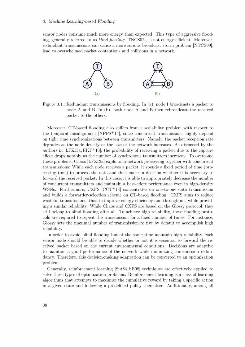
3. Machine Learning-based Flooding
sensor nodes consume much more energy than expected. This type of aggressive flood-ing, generally referred to as blind flooding [TNCS02], is not energy-efficient. Moreover,redundant transmissions can cause a more serious broadcast storm problem [NTCS99],lead to overwhelmed packet contentions and collisions in a network.
I
BA
(a)
I
BA
(b)
Figure 3.1.: Redundant transmissions by flooding. In (a), node I broadcasts a packet tonode A and B. In (b), both node A and B then rebroadcast the receivedpacket to the others.
Moreover, CT-based flooding also suffers from a scalability problem with respect tothe temporal misalignment [NPPS+15], since concurrent transmissions highly dependon tight time synchronizations between transmitters. Namely, the packet reception ratedegrades as the node density or the size of the network increases. As discussed by theauthors in [LFZ13a,RKP+16], the probability of receiving a packet due to the captureeffect drops notably as the number of synchronous transmitters increases. To overcomethese problems, Chaos [LFZ13a] exploits in-network processing together with concurrenttransmissions: While each node receives a packet, it spends a fixed period of time (pro-cessing time) to process the data and then makes a decision whether it is necessary toforward the received packet. In this case, it is able to appropriately decrease the numberof concurrent transmitters and maintain a best-effort performance even in high-densityWSNs. Furthermore, CXFS [CCT+13] concentrates on one-to-one data transmissionand builds a forwarder-selection scheme on CT-based flooding. CXFS aims to reducewasteful transmissions, thus to improve energy efficiency and throughput, while provid-ing a similar reliability. While Chaos and CXFS are based on the Glossy protocol, theystill belong to blind flooding after all. To achieve high reliability, these flooding proto-cols are required to repeat the transmission for a fixed number of times. For instance,Glossy sets the maximal number of transmission to five by default to accomplish highreliability.In order to avoid blind flooding but at the same time maintain high reliability, each
sensor node should be able to decide whether or not it is essential to forward the re-ceived packet based on the current environmental conditions. Decisions are adaptiveto maintain a good performance of the network while minimizing transmission redun-dancy. Therefore, this decision-making adaptation can be converted to an optimizationproblem.Generally, reinforcement learning [Sut84, SB98] techniques are effectively applied to
solve these types of optimization problems. Reinforcement learning is a class of learningalgorithms that attempts to maximize the cumulative reward by taking a specific actionin a given state and following a predefined policy thereafter. Additionally, among all
38

3.1. Introduction
the reinforcement learning techniques, a set of so-called multi-armed bandit algorithmsis particularly suitable for the optimization of CT-based WSNs. That is because thenumber of transmissions in each sensor node can be furthermore modeled as a multi-armed bandit problem, originally described by Robins [Rob85].
A multi-armed bandit, also called K-armed bandit, is similar to a traditional slotmachine but generally with more than one lever. As further explained by Auer etal. [ACBFS95], in a multi-armed bandit problem, a gambler need to choose which of slotmachines to play. At each time step, the gambler pulls the arm of one of the machines.After that, he receives a reward or a payoff. The purpose is to maximize the total rewardover a sequence of trials. Therefore, the goal is to find the arm with the best expectedreturn as early as possible, and then to keep gambling using that arm, since each arm isassumed to have a different distribution of rewards. Similarly, this type of multi-armedbandit algorithm investigates the selection of the “best” action for the dynamic situationsin low-power and lossy WSNs as well.
We propose Less is More (LiM), a machine learning-based data dissemination proto-col for low-power multihop WSNs. In designing LiM, we utilize a reinforcement learningtechnique to reduce redundant broadcast transmissions. We model the optimization ofthe transmission times in each sensor node as a multi-armed bandit problem. Besides, weexploit an exponential-weight algorithm for exploration and exploitation (called Exp3 ),for bandit learning in each sensor node of the WSN. Incorporated with concurrent trans-missions, LiM is able to effectively achieve high end-to-end reliability and low end-to-endlatency. Moreover, LiM empowers sensor nodes with a learning capability to reduce theredundancy of the flooding step by step, thereby significantly lowering power consump-tion. We implement LiM in Contiki [DGV04] and conduct extensive experiments in a30-node testbed — FlockLab [LFZ+13b]. Furthermore, we compare LiM to the baselineprotocol Glossy [FZTS11] focusing on reducing communication redundancy in flooding.
Our evaluation shows that LiM is able to effectively limit the number of transmissionsof the sensor nodes while still preserving high reliability and energy efficiency, as well aslow latency: Sensor nodes, which do not belong to the backbone of the network, stay onlyin receiving and sleeping mode. The others execute the decision-making based on theirobtained experience from the learning phase. With various levels of transmission (TX)power and different topologies, LiM obtains an average reliability of over 99.70% and anaverage end-to-end latency of less than 2.4 ms in all experimental scenarios. Moreover,LiM reduces the radio-on time by at least 30% compared to the default configuration ofGlossy.
The remainder of this chapter is organized as follows. Section 3.2 discusses relatedwork with two foci: on Glossy-based flooding protocols and on bandit-learning strategiesapplied in WSNs. Section 3.3 explains the basis of LiM and provides a brief overview.Section 3.4 details the design perspectives of LiM, followed by performance evaluationselaborated in Section 3.5. Section 3.6 concludes our work and leads to an outlook forfuture work.
39

3. Machine Learning-based Flooding
3.2. Related Work
In this section, we review a number of existing research work in terms of CT floodingprotocols in WSNs, multi-armed bandit algorithms, and the bandit learning in WSNs.
3.2.1. CT-based Flooding Protocols
Network flooding is one of the most fundamental services in WSNs. It forms the basis fora wide range of applications and network operations. Glossy [FZTS11] provides a fastand efficient network flooding service by using concurrent transmissions in WSNs. Byexploiting constructive interference and the capture effect on the physical layer, Glossyis able to get an average packet delivery ratio of 99.99% in real testbeds. Afterwards,Ferrari et al. adds an application-level scheduler to construct a so-called Low-powerWireless Bus (LWB) [FZMT12]. LWB centrally schedules the data communication tosupport one-to-many, many-to-one, and many-to-many traffic patterns in WSNs. Onthe contrary, Chaos [LFZ13a] builds on Glossy to achieve fast all-to-all data sharing in adistributed manner. Chaos further combines programmable in-network processing withconcurrent transmissions in WSNs.Splash [DCL13] builds a tree pipeline [RCBG10] on Glossy, thereby improving channel
utilization. Furthermore, Pando [DLZL15] integrates fountain code [Mac05] togetherwith CT and disseminates packets as data pipelines so as to overcome the long-tailproblem of Splash. While Glossy disseminates one packet in each communication round,Splash and Pando are designed to deliver large data objects to all nodes in a network,e.g., an up-to-date image for the purpose of reprogramming WSN-based applications.Ripple [YH15] also relies on Splash and network coding techniques to further improveparticularly in terms of network throughput.Carlson et al. propose CXFS [CCT+13], a forwarder selection mechanism for con-
current transmissions. In CXFS, sensor nodes use a hop count in each packet to gettheir relative distance to each other. CXFS builds on Glossy and supports point-to-point transmissions while achieving high reliability, high energy efficiency, and highthroughput. Moreover, Sparkle [YRH14] selects subsets of nodes that participate inGlossy-based flooding. It also supports one-to-one communication. Similarly, Lane-Flood [BLS16] is built on Glossy and further integrates the forwarder selection scheme ofCXFS with application-level network protocols in WSNs. LaneFlood thus supports one-to-one traffic, forwarder selection, and standard protocols in IoT such as TCP/UDP andthe Constrained Application Protocol (CoAP). RTF [ZRHK15] further extends Sparkleand exploits TDMA for data scheduling to improve reliability and energy efficiency inpoint-to-point traffic. RFT identifies reliable relay nodes to limit the number of concur-rently active neighbors to save more energy.
3.2.2. Multi-armed Bandit Algorithms
Many real-word problems require decisions to be made for maximizing the expectedreward. Over the last two decades, a number of algorithms have been designed for thispurpose.One simple strategy, called ε-greedy, was first investigated by Watkins [Wat89]. This
40

3.2. Related Work
method introduces an ε-frequency, which is configured by the users, to decide the prob-ability of uniformly trying an action. Otherwise, the algorithm executes the action withthe highest mean value µ. The Exp3 algorithm [ACBFS95], first introduced by Auer,considers using a modified softmax function to decide the possibility of trying differentactions.Besides, several more strategies were proposed after ε-greedy and Exp3. For instance,
in 1998, Cesa-Bianchi et al. introduced SOFTMIX [CBF98]. In 2005, Vermorel etal. introduced the POKER algorithm [VM05]. These algorithms are claimed to performbetter than ε-greedy and Exp3. However, compared to the others, Exp3 is simple, widelyused, and easy to be implemented on an embedded sensor device, especially running onContiki OS. In this work, we select the Exp3 algorithm as a candidate (i) to provethe feasibility of reinforcement learning algorithms in resource-constrained sensor nodes,and (ii) to evaluate the usability and adaptability of this kinds of learning algorithms inWSNs.
3.2.3. Bandit Learning in WSNs
In [MB07], Motamedi et al. propose a distributed multi-channel MAC protocol for wire-less networks. It formulates the dynamic channel selection in wireless networks as amulti-armed bandit problem and derives optimal channel selection rules. The authorsinvestigate the effectiveness of their protocol by using simulations only. Thus, the effec-tiveness in real-world scenarios is therefore not clear.Similarly, another multi-channel access scheme is proposed in [ZSJS16] to schedule the
access for cognitive users, in order to maximize the throughput in cognitive radio-basedWSNs. By their simulation results, the authors claim that the proposed scheme caneffectively improve the utilization of the idle spectrum and guarantees the fairness ofselecting channels between cognitive users.In [KF14], Kadono et al. propose a budget-limited multi-armed bandit algorithm,
which is suitable for resource-constrained WSNs. It can limit sources to be retrievedwhen a relatively hard budget limitation has been applied. By conducting simulations,the authors claim that the proposed protocol outperforms the state-of-the-art.Authors in [dPAP12] present a duty cycle learning algorithm (DCLA) for IEEE
802.15.4 WSNs. DCLA automatically adapts the duty cycle during run-time to mini-mize power consumption and to balance the packet delivery ratio and delay constraintsof the application. It estimates the incoming traffic by collecting network informationduring each active phase and then uses a reinforcement learning framework to learn thebest duty cycle at each beacon interval. Simulations demonstrate that the proposedscheme achieves the best overall performance for both, constant and event-based traffic,compared to existing IEEE 802.15.4 duty-cycled adaptation schemes.In [TTRJ12], the authors study the long-term information collection in the WSN
domain. They propose a multi-armed bandit-based approach for the energy managementproblem in WSNs. They also describe a multi-armed bandit algorithm — Exp3 — thatcan be used to efficiently deal with the energy management problem. They show throughsimulations that their approaches improve the performance of the network by up to 120%.
In [VRP12], Villaverde et al. present a route selection algorithm (InRout), whichshares local information among neighboring nodes to enable efficient, distributed route
41

3. Machine Learning-based Flooding
selection. They model it as a as a multi-armed bandit problem and use Q-learningtechniques to obtain the best routes based on current network conditions and applicationsettings. The authors compare InRout with existing approaches by simulations. Theirresults demonstrate that InRout provides gains ranging from 4% to 60% in the numberof successfully delivered packets compared to current approaches while having a lowercontrol overhead.
3.2.4. Summary
Concurrent transmissions — a promising technique in this field — allow highly energy-efficient, low-power communication in WSNs. The technique has been developed andintegrated with different standards and techniques. None of the state-of-the-art pro-tocols, however, makes a great effort to apply an adaptive machine-learning scheme toconcurrent transmissions. On the other hand, the bandit-learning scheme has been ex-ploited in the field of WSNs for smart duty cycling, long-term energy management, androute selection. Most of the work has been investigated by using simulations only. As aconsequence, their effectiveness in real-world scenarios has not been shown yet.LiM incorporates concurrent transmission with a bandit-learning scheme in order to
take advantage of both techniques. Meanwhile, LiM proves the feasibility of apply-ing relatively light-weight machine-learning techniques to concurrent transmission forlow-power wireless networks in real-world applications. To the best of our knowledge,LiM is the first primitive that integrates a machine-learning scheme with concurrenttransmissions, especially for low-power multihop WSNs. We believe that LiM is ableto be further developed to robustly resist more adverse conditions in reality, e.g., witha channel hopping scheme in [ZLT17], and to satisfy the requirements of the variousapplications.
3.3. Overview
In this section, we explain the basis of LiM in two dimensions: (i) reliable flooding and(ii) machine leaning. Then, we provide a brief overview of the protocol.
3.3.1. Reliable Flooding
Proposed in 2011, Glossy [FZTS11] is one of the most representative CT-based floodingprotocols in the WSN community. Basically, Glossy exploits both, constructive interfer-ence to superimpose (identical) packets and the capture effect to ensure that a receiveris actually able to correctly demodulate a received packet. These two mechanisms em-power Glossy to manage a highly reliable flooding and an accurate time synchronization.In Glossy, nodes concurrently transmit packets in a receive-and-forward scheme, whichmeans that nodes receive a valid packet and forward it immediately. Messages are prop-agated through the network without contention of the wireless medium. Therefore, thelatency of flooding could approximately reach the theoretical upper bound, as studiedin [FZTS11]. Moreover, nodes in the network get clock-synchronized to the initiator inorder to estimate the time to wake up, thereby saving much energy.
42

3.3. Overview
Figure 3.2 demonstrates one Glossy flooding example. The network consists threenodes, which are highly time-synchronized among each other. Node I can reach node Abut not B, and node B can reach node A but not I, as shown in the figure. Nodes areconfigured with the number of transmissions equals to two, i.e. N = 2, which meanseach node only transmits the packet twice in total. At first, node I starts to send apacket to node A in time slot 0, as a normal transmission. After node A has successfullyreceived the packet, it transmits the packet to both, node I and B in time slot 1. Intime slot 2, as node I and B have received the packet, both of them synchronously sendthe packet to node A, as concurrent transmissions. At the end of this time slot, nodeI finishes two transmissions and goes into a sleep mode. In time slot 3, node A sendsthe packet to node B and then goes to sleep. Node B receives the packet in time slot4. Afterwards, it sends the received packet again and goes to sleep. At the end, onedata packet from node I has been reliably disseminated to each node in the network forseveral times.
I
A
B
TX
RX TX RX TX
RX TX
Time Slot 0 1 2 3 4
TX
Transmission
RX
ReceivingRadio-on period
Concurrent transmission
Normal transmission
Time
RX TX RX TX
Figure 3.2.: Example of a Glossy flooding round with N = 2 in a topology of threenodes. Black lines connecting the nodes imply the communication links.Each node transmits only twice in total. Nodes always concurrently transmitpackets once they have received them. Thin arrow lines stand for a normaltransmission, where CT does not exist to the receiver. Thick arrow linesrefer to a CT, where occur the constructive interference and the captureeffect to the receiver.
3.3.1.1. Constructive Interference
In physics, interference is a phenomenon in which two or more waveforms superpose toform a resultant wave, which is either reinforced or canceled. As shown in Figure 3.3(a),constructive interference is generated from the two identical waves 1 and 2, which leadsto a wave of greater amplitude. Otherwise, destructive interference is created when thetwo waves cancel each other, thus resulting a wave of weaker amplitude, as shown inFigure 3.3(b).Specifically, in WSNs, constructive interference occurs only when two or more nodes
43

3. Machine Learning-based Flooding
transmit identical packets. Besides, it requires a highly tight time synchronizationsamong radio transmitters. For instance, with IEEE 802.15.4 radios operating in the2.4 GHz ISM band, these identical packets from various transmitters are required tooverlap within 0.5 µs [DDHC+10,FZTS11] in order to make the packets appropriatelysuperposed.
Resultant Wave
Wave 1
Wave 2
(a)
Resultant Wave
Wave 1
Wave 2
(b)
Figure 3.3.: Constructive interference and destructive interference resulted from twowaves.
3.3.1.2. Capture Effect
The capture effect, also referred to as co-channel interference tolerance, is a phenomenonwhere a certain radio correctly receives a strong signal from one transmitter despitesignificant interference from other transmitters [LF76, WWJ+05]. In IEEE 802.15.4wireless networks, if a received signal is approximately 3 − 4 dB stronger than thesum of all the other received signals, then the receiver is able to lock on to and correctlydemodulate the signal [LF76,WWJ+05,FZTS11]. Additionally, the strongest signal mustarrive no later than 160 µs after the weaker signals in order to be properly captured anddecoded by the receiver [LFZ13a]. In other words, within a time period of 160 µs, ifthere are multiple signals transmitting to a receiver, then the strongest signal wins thechance to be correctly received. Accordingly, the others are considered as interference.
3.3.2. Machine Learning
Machine learning is a sub-field of artificial intelligence that is concerned with the questionof “how to construct computer programs that automatically improve from experience”[Mit97]. This property makes the family of machine learning-based algorithms attractivefor reliable and efficient communications in WSNs.
44

3.3. Overview
3.3.2.1. Reinforcement Learning
Reinforcement learning is one of the machine-learning techniques, in which the learningagent earns knowledge from the interaction with the environment. Technically, reinforce-ment learning is used by a class of algorithms that seeks to maximize the cumulativereward by executing different actions in a task. In this case, different configurations ofa system can be modeled as the corresponding actions to maximize the reward in orderto optimize the performance of the system.
3.3.2.2. Multi-armed Bandit Problem
The multi-armed bandit problem was originally proposed by Robbins [Rob85] in theyear of 1985. A gambler, firstly, chooses K slot machines to play. At each time step, thegambler pulls one arm of one machine (out of K) and then receives a positive, zero, ornegative reward. The purpose is to maximize the total reward over a sequence of trials.Assuming each arm in a slot machine has a different distribution of rewards, the goal isto find out the arm with the best expected return as early as possible and then to keepusing that specific arm.The problem is a classical example of the trade-off between exploration and exploita-
tion [ACBFS95]: On the one hand, if the gambler plays exclusively on the machine whichthe gambler supposes to be the best one (“exploitation”), then the gambler may fail todiscover that one of the other arms, in fact, has a higher average return. On the otherhand, if the gambler spends too much time trying out all K machines and then makesa decision based on the gathered statistics (“exploration”), then the gambler may fail toplay the best arm for long enough a period of time to get a high total return.To solve the multi-armed bandit problem, the Exponential-weight algorithm for Ex-
ploration and Exploitation (Exp3) was proposed by Auer et al. [ACBFS02] in the yearof 2002. Exp3 is based on a reinforcement learning scheme and it solves the followingproblem:
“If there are many available actions with uncertain outcomes in a system, howshould the system act to maximize the quality of the results over many trials? ”
We provide the details of Exp3 and the related implementation issues later in Section 3.4.
3.3.3. LiM in a Nutshell
LiM builds on Glossy and it is able to effectively inherit the advantages of the CT-basedflooding protocols, i.e., high reliability, low latency, and low radio duty cycle. In thiscase, LiM exploits both, constructive interference and the capture effect to guarantee agood performance of the network. Meanwhile, it is challenging to integrate LiM withGlossy, since Glossy requires a highly tight deterministic software delay and the identicalcontent of the packet for concurrent transmission.The feedback from the neighboring nodes should be renewed according to the dynamic
network conditions, leading various packets within the network. Therefore, the require-ment of identical content of the packets cannot be satisfied. However, the packets inLiM are not necessarily identical, since LiM opportunistically uses the capture effect to
45

3. Machine Learning-based Flooding
effectively receive the packet with the strongest signal level. Additionally, LiM mod-els the redundancy optimization problem as a multi-armed bandit problem and maps anumber of configurations to the corresponding actions in each sensor node. LiM employsa bandit-learning scheme — Exp3 — in order to progressively optimize the efficiency ofthe network. This learning scheme investigates the selection of the “best” action for thedynamic environment, dramatically minimizing the redundancy of the communicationswhile still maintaining a high reliability.Generally, LiM comprises two main phases: a greedy exploration phase and a bandit
learning phase. The former one is an exploration process where the “redundant” nodesin the network could be discovered. In this phase, LiM randomly selects one node toact as a exploring node in the network. This exploring node triggers some unexpectedevents in the network, e.g., after receiving a packet from its “upside” parent nodes, itstops forwarding for some time slots. As a result, a number of communication linksare disabled during those time slots. Some neighboring nodes might suffer a packet lossfor this period of time and accordingly they give negative feedback to the exploringnode. Otherwise, if no one suffers a packet loss, then the exploring only receives positivefeedback and then LiM regards this exploring node as a “redundent” node. This type of“redundant” nodes acts as a concurrent transmitter in CT-based protocols. LiM attemptsto seek these nodes and then keeps them staying in either receiving mode or sleepingmode in the network. Therefore, it is able to reduce redundancy and to improve theenergy efficiency of the network.The latter phase is a reinforcement learning process. Similar to the exploration phase,
in the learning phase, LiM attempts to grant each node (except the previous found“redundant” node) to select a corresponding action (i.e., the number of transmission (N))based on the network dynamics. This selection depends on the result of the reinforcementlearning in each node — choosing the action with the highest probability. Moreover, thelearning phase has no conflict with data dissemination, which means, in this phase, LiMconcurrently floods the information while progressively learning from the dynamics. Inthe following section, we explain these two phases of LiM in more detail.
3.4. Design of LiM
In this section, we detail the design aspects of LiM. We discuss the basis of LiM: con-current transmissions and the reinforcement learning scheme, respectively. Besides, wedepict two phases of LiM in detail.
3.4.1. Concurrent Transmissions
As derived from Glossy, LiM is based on CT, i.e., constructive interference and the cap-ture effect. LiM adds an action scheme together with a feedback scheme to progressivelylearn the dynamics of the network. The feedback scheme is based on one specific byte ineach packet updated by the neighboring nodes of a node. In the following, We specify thedesign of the frame structure in LiM. As a consequence, the content of a packet cannotbe guaranteed to be identical all the time. By exploiting the capture effect, however, thereceiver is able to correctly receive a packet with the stronger signal strength. In othercases, LiM similarly works with constructive interference as Glossy.
46

3.4. Design of LiM
Figure 3.4 shows the protocol stack of LiM. LiM operates IEEE 802.15.4 radios (i.e.,CC2420) on the physical layer which is integrated with Glossy. On the MAC layer,LiM incorporates a machine learning module on the top of Glossy. That is, the learningmodule helps to update the feedback based on CT. Meanwhile, the parameters in CT(i.e. Glossy) are configured based on the actions determined by the learning results. Asa result, LiM can be considered as an extension of Glossy, namely, it builds the learningscheme consisting of feedback and action selection on a higher layer of Glossy. Theapplication layer can be further developed to meet the users’ requirements, for instance,data dissemination. Later in this section, we explain the action and the feedback schemein more detail.
Glossy
CC2420 Radio
Application
Learning
PHY
MAC
APP
FeedbackAction
Figure 3.4.: Protocol stack of LiM. LiM builds on CC2420 radio as a physical layer andintegrates Glossy on the MAC layer. It exploits an iterative reinforcementlearning scheme to select an action based on the feedback. Arrows in thefigure refer to the interactions between different layers.
3.4.1.1. Number of Transmissions
By design, LiM maps four configurations of transmission times to four actions respec-tively: Action 0 stands for a node staying only in receiving (i.e., LPL) or sleeping mode,i.e., N = 0; Action N (N = 1, 2, 3) means that a node works normally except settingthe maximal transmission times to N , i.e., transmitting the packet N times. In general,nodes in LiM exploit one of the above-mentioned four actions to effectively reduce thebroadcast times in order to improve energy efficiency. Besides, the initiator in LiM isexempted from the action selection. Namely, the initiator maintains the default maximalnumber of transmission (i.e., N = 5, the same as Glossy), and does not execute neitherthe greedy exploration phase nor the bandit learning phase.
3.4.1.2. Frame Structure
To support the feedback scheme, LiM extends the frame structure in Glossy by addingone byte for an exploring ID field and one byte for a feedback field, respectively. One
47

3. Machine Learning-based Flooding
example of a frame structure is illustrated in Figure 3.5.
Frame Length Header Data Relay
Counter CRCFeedbackExploring ID
1 1 4 1 1 1 2Bytes:
Field:
Figure 3.5.: Application-level frame structure in LiM. By design, the length of the datafield (payload) is set to eight bytes in LiM. The exploring ID field is to notifythe nodes in the network to proceed to different phases. The feedback fieldis to carry a response for the learning process.
The frame length stands for the length of the whole frame in bytes. The header isa constant value, e.g., 0xA0 in LiM. The length of the data (i.e., payload) in LiM canbe adjusted according to the needs of different applications. By default, LiM sets thepayload length to eight bytes. The exploring ID field is to disseminate the ID of thecurrent exploring node: A node that receives the packet is able to notice whether it isthe right time for itself to explore or to learn. While a node experiences a packet loss,the feedback field is in use and is updated to a negative feedback value. If not, thefeedback is not updated after the data packet has been received from the upper-levelnodes, and hence, remains a positive feedback value. The relay counter is inherited fromGlossy for concurrent transmissions and time synchronization. A Cyclic RedundancyCheck (CRC) is an error-detection field to discover accidental changes to the raw datawhile transmission in the air.
3.4.1.3. Feedback Scheme
The feedback scheme is one key feature of LiM. Namely, only with the accurate feedback,nodes can make the correct decision of choosing the appropriate action according to thenetwork dynamics.As mentioned in Section 3.3, LiM consists of two main phases: an exploration phase
and a learning phase. The former one is an exploration process where the “redundant”nodes can be discovered so as to reduce the redundant broadcasts. LiM attempts toseek these nodes and then keeps them staying in either receiving mode or sleeping modein the network. The second phase is a reinforcement learning process. In this phase, anode in LiM floods the information and updates the corresponding actions based on thefeedback received from the network, thereby, progressively learning from the dynamics.To achieve the accurate feedback from neighboring nodes, a node in LiM assigns two
types of feedback: a positive feedback (0x01) and a negative feedback (0x00). When anode is in the exploration phase, then it explores whether it is a “redundant” node or not,for instance, node A in Figure 3.2. At first, it stops forwarding the received packets in thecurrent transmission round. As a result, the neighboring nodes, i.e., child node node Band parent node I in Figure 3.2, suffer a packet loss in the current round and accordinglyupdate the feedback byte to a negative one (0x00). In the following round, as a newflooding round comes from node I, the exploring node recovers to receive and forwardpackets. In this case, it receives the packet with the negative feedback byte written bythe neighboring nodes, which have lost a packet in the previous round. Correspondingly,the exploring node, i.e. node A, reads the feedback byte in the packet and then (iii)
48

3.4. Design of LiM
makes a corresponding decision base on the feedback.When in the bandit learning phase, the criterion is similar to the one in the exploration
phase. If a node is in a learning phase, then it attempts to use different configurationsof number of transmissions (N) for each round. Besides, if the neighboring nodes ofthis node receive at least one packet, then the neighboring nodes update the feedbackbyte as a positive one (0x01) in the packet. Otherwise, they renew the feedback byteto a negative one (i.e. 0x00). Afterwards, they continue to forward the packet with theup-to-date feedback byte. The learning node subsequently receives the packet and thenuses learning algorithm to compute the probability distribution of each action based onthe received feedback. After that, the node chooses the corresponding action with thehighest probability.In a few cases, the capture effect could fail to work correctly due to the density of
the nodes [LFZ13a]. Another reason is, that the feedback byte from different nodeis different. For example, when in learning phase, if a positive feedback from “upside”parent node and a negative one from “downside” child node are concurrently transmittedto this learning node, then this could cause an invalid packet so that the feedback is notaccurate any more. To overcome this situation, LiM extends one extra listening timeslot particularly for the packets from child nodes to obtain a correct feedback, e.g., nodeB, as shown in Figure 3.6. Figure 3.6 reveals the timeline of one single round in theflooding protocol. In time slot 6, with N = 3 node B should have gone to sleep modebecause it had already transmitted three times in this flooding round. However, since itis in the leaning phase in this round, it keeps listening in time slot 6 and receives an extrapacket from its child node, i.e., node C. In next sections, we explain the exploration andlearning phases in more detail.
3.4.2. Greedy Exploration
In general, there are two main phases in LiM: (i) a greedy exploration phase and (ii) abandit learning phase. In this section, we detail the exploration phase in LiM.In LiM, after a node is powered on, the first step is, that it keeps its radio on and
listening to the communication channel. Meanwhile, a so-called “initiator ”, consideredas the information source of a flooding, starts broadcasting packet periodically, similarto Glossy. As a result, the other nodes, which are currently listening, are able to receivethe packet from the initiator hop-by-hop. Afterwards, based on the time-stamp of the re-ception, a node accomplishes time synchronization with the node (its parent node) fromwhich the packet comes. When each node in the network is synchronized, the initial-ization of the network is then achieved. This is guaranteed by the time synchronizationscheme derived from Glossy [FZTS11].Next, LiM comes to an exploration phase. In this phase, LiM aims to explore the nodes
that are not essential for transmitting or forwarding the received packets in the network,i.e., so-called “redundant” nodes. We define this type of nodes as “absorbing nodes”that can always stay in either receiving mode or sleeping mode, but not in transmittingmode. Due to the special characteristics of these nodes, the number of absorbing nodessignificantly affects the performance of the CT-based flooding protocols, e.g., floodingredundancy.Determining the trade-off between the number of absorbing nodes and the network
49

3. Machine Learning-based Flooding
I
A
B
C
D
TX
RX TX
RX
RX TX RX TX
RX TX RX TX
TX RX TX RX TX
RX TX RX TX RX TX
RX TX RX TX RX TX
Time Slot 0 1 2 3 4 5 6 7
RX
TX
Transmission
RX
ReceivingRadio-on period
Concurrent transmission
Normal transmission
Time
RX
Additional receiving slot
Time...
Flooding round
... ... ...
Figure 3.6.: Example of a LiM flooding round with a configuration ofN = 3 in a topologyof five nodes. A data packet is generated in and flooded from node I to allthe others. In this round, node B is in a learning phase. LiM compelsnode B to extend one extra listening time slot for the exploring feedback,particularly for receiving the feedback from child node (i.e., node C).
reliability is quite critical. On the one hand, increasing the number of absorbing nodesdecreases the number of concurrent transmitters, consequently strengthening the concur-rent transmissions in the network, according to the results in [LFZ13a]: The reliability(i.e., PDR) degrades greatly with the increasing number of concurrent transmitters. Onthe other hand, maintaining too many absorbing nodes might lead to a fragile networkwith a higher probability that nodes get disconnected while the environment dynamicallychanges or the interference suddenly gets harsh.LiM appropriately explores the absorbing nodes by considering the dynamical envi-
ronment in the exploration phase, as depicted in Algorithm 1. At first, the initiatorgenerates an exploring list L containing all the node IDs of the whole network, exceptthe initiator itself. Then, the initiator selects one node ID from the exploring list andwrites it into the “Exploring ID” field of the data packet (see Figure 3.5). Next, theinitiator disseminates this packet for a number of consecutive flooding rounds, e.g., bydefault with a configuration of f = 10 for each single ID in LiM. Then, the initiatorremoves the ID of the exploring node from the list L. If the exploring list is empty, thenthe initiator learns that the phase of exploration is complete.When a node is assigned to be an exploring node by the initiator, it receives a packet
50

3.4. Design of LiM
that contains its own node ID in the “Exploring ID” field. Thereby, in the current floodinground, it only receives the packets from the neighboring nodes but does not forward anypacket, i.e., it acts as an absorbing node. Afterwards, in the following flooding round,the node recovers as a normal node, i.e., it continues to forward the received packetsand meanwhile receives the feedback from neighboring nodes — whether they have lostany packet or not. Correspondingly, the node checks the feedback byte of the receiveddata packet and then makes a decision based on the received feedback: If it is negative,then the node considers itself as an essential node in the network; otherwise, the nodeconsiders itself as an absorbing node.Generally, if neighboring nodes of the exploring node lose any packet in the current
flooding round, then they update the feedback byte to a negative one (i.e. 0x00) in theirreceived packet and transmit it in the following flooding round. In this case, the exploringnode is able to make a decision in the next flooding round based on the feedback fromits neighboring nodes.
Algorithm 1 Exploration1: procedure Initialization2: initialize a node ID list: L3: end procedure4: procedure Iteration5: for L is not empty do6: select a node ID ni ∈ L7: update the “Exploring ID” byte in the packet with ni8: trigger f consecutive rounds of flooding9: remove node ID ni from L10: end for11: end procedure
Figure 3.7 demonstrates an example after greedy exploration in LiM. Compared to theprevious topology shown in Figure 3.6, node B is in the first hop from the initiator, actingas as the child node of node I and the parent node of node C. While in the explorationphase, node B finds out that it is not necessary for itself to forward the received packetto the neighboring nodes. Since with or without it, the neighboring nodes do not loseany packet. Node B decides to act as an “absorbing node”, i.e., staying only in receivingmode or sleeping mode, thereby, the link between node B and node C is removed bynode B, as shown in Figure 3.7.Specifically, in LiM, if a node decides to be an absorbing node, then it extends one more
slot for LPL on the occasion that it misses the packet in the first slot. This is because,that the time synchronization inherited from Glossy is not fine-grained — it is highlydependent on the clock in CC2420 radio [FZTS11]. Beside, after the exploration phase,a node, once being considered as an absorbing node, can only listen to the channel andreceive a packet in the first time slot. In this case, if the clock drifts in an absorbing node,this node might lose the chance to receive any packet, since the time synchronizationis not accurate any more and accordingly the node misses the first time slot — itsonly chance to receive. To overcome this problem, LiM extends one more time slot forlistening so as to add a period of guard time, e.g., node B shown in Figure 3.7. It
51

3. Machine Learning-based Flooding
guarantees, that node B has enough time slot to receive a packet regardless of the clockdrift problem.Please note, that in the exploration phase, the initiator in LiM by default does not
transmit any real data in the payload except the node ID, since the probability of packetloss is relatively high. However, if users can tolerate the loss, then the initiator can beset to transmit real data also in this exploration phase. With respect to this point, weshow the reliability of LiM particularly in the exploration phase later in Section 3.5.
I
A
B
C
D
TX
RX TX
RX
RX TX RX TX
RX TX RX TX
RX TX RX TX RX TX
RX TX RX TX RX TX
Time Slot 0 1 2 3 4 5 6 7
TX
Transmission
RX
ReceivingRadio-on period
Concurrent transmission
Normal transmission
Time
Figure 3.7.: Example of a LiM flooding round with a configuration ofN = 3 in a topologyof five nodes. Nodes self-prune the connection links during the explorationphase. Node B (in yellow) then acts as an absorbing node and stays inreceiving mode in a flooding round. In this example, node B attempts toextend the listening time for one more time slot, in case that it misses thepacket in slot 0. As a result, node B still saves the energy consumed in fourslots compared to the other nodes.
3.4.3. Multi-armed Bandit Learning
Similar to the exploration phase, in the learning phase, LiM attempts to grant each node(except the previous found “redundant” node) to select a corresponding action, i.e., thenumber of transmission (N ). The selection is based on the result of the reinforcementlearning in each node — choosing the action with the highest probability. Moreover, thelearning phase has no conflict with data dissemination, which means, in this phase, LiMconcurrently floods the information while progressively learning from the dynamics. Inthis section, we detail the learning phase in LiM.Firstly, we explain the main bandit learning algorithm. As different configurations
52

3.4. Design of LiM
are mapped to responding actions, we model the optimization problem as a multi-armedbandit problem. In order to overcome this problem, we use one algorithm from the setof multi-armed bandit learning algorithms: Exp3. In our case, the goal of the algo-rithm is to optimize the energy efficiency with reliability based on the policy of selectingtransmission times for each sensor node.Considering a process withK different actions, the Exp3 algorithm functions as shown
in Algorithm 2, where γ is the so-called exploration factor and wi is the weight of eachaction i. pi(t) is the probability of selecting action i in flooding round t, and xi(t) ∈ [0, 1]is the reward of action i on flooding round t, while T means the total number of iterations.At the beginning, the algorithm initializes the exploration parameter γ. This param-
eter adjusts the possibility that the algorithm attempts to explore other actions while acertain action has already achieved the highest probability, i.e., trying new actions re-gardless the one with converged probability. Next, the algorithm associates a weight witheach action in order to give each action a probability to form a probability distributionP over all actions.
Algorithm 2 Exp31: procedure Initialization2: initialize γ ∈ [0, 1]3: initialize the weights wi(1) = 1, ∀i ∈ {1, . . . ,K}
4: set pi(t) = (1− γ)wi(t)∑Kj=1wj(t)
+γ
K, ∀i ∈ {1, . . . ,K} for the distribution P
5: end procedure6: procedure Iteration7: for t < T do8: draw the next action it randomly according to the distribution P9: observe the reward xit(t)10: define the estimated reward x̂it(t) = xit(t)/pit(t)11: set the weight of action it: wit(t+ 1) = wit(t)e
γx̂it (t)/K
12: set all other weights: wj(t+ 1) = wj(t), ∀j 6= it and j ∈ {1, . . . ,K}
13: update P: pit(t+ 1) = (1− γ)wit(t+ 1)∑Kj=1wj(t+ 1)
+γ
K, ∀it ∈ {1, . . . ,K}
14: end for15: end procedure
After the exploration phase, the algorithm iterates T times the learning procedure inorder to learn from the environment and to generate an accurate probability distributionto receive more accumulative rewards, so that the probabilities of various actions can haveenough time to be converged. In the iterative learning procedure, at first, the algorithmrandomly selects an action it as the next executive action based on the distributionP. Then, it executes the action it, and receives a reward xit(t) from the environment.Specifically, hereby in LiM, the reward from the environment implies the feedback fromneighboring nodes in the network. Thereafter, an estimated reward x̂it(t) is calculatedas xit(t)/pit(t) to further include the influence of the probability on the reward. In theend, the weight of the sampled action is updated, while the weights of other actions
53

3. Machine Learning-based Flooding
(wj , ∀ j 6= it, j ∈ {1, . . . ,K}) remain unchanged. While the algorithm converges,the eventual probability distribution P over different actions is considered to be theguidance to select the best action in order to maximize the reward.
To integrate Exp3 in LiM, each action in this algorithm is associated with a cor-responding configuration in each node, which is mentioned in Section 3.4.1. In eachiteration, the probability of selecting a certain action is calculated based on the feedbackfrom the neighboring nodes. For instance, there are three actions (K = 3) in the learningprocedure of LiM by design, i.e., action 1, 2, and 3. Respectively, action 1, 2, and 3 aremapped to three different configurations, where nodes transmit the packet once, twiceor three times, respectively. That is, if the randomly sampled action i is 1, then thenode only transmits once in the current round. After the node receives the feedback,the weight of the corresponding action (i.e., action 1) is updated as shown in Line 11of the algorithm. The weights of other actions (i.e., action 2 and 3) stay the same (inLine 12). In the final step, the distribution P is updated to prepare for the next iterativeflooding round according to the formula in Line 13 of the algorithm.
At this point of time, one learning iteration has been performed. This iteration phasecontinues until the number of flooding rounds reaches T . By design, LiM sets this valueto T = 200, i.e., a fixed learning period for each node in LiM. However, due to thedynamic environmental changes, a fixed period might cause a case that the probabilityof choosing an action does not converge. We detail and evaluate this case later inSection 3.4.4.2.
Similar to the greedy exploration phase depicted in Algorithm 1, the initiator main-tains an exploring list L containing all IDs of the nodes in the whole network, except theinitiator itself and the absorbing nodes. Here in the learning phase, f equals to T , i.e.,200 consecutive flooding rounds. After the learning phase of one particular node (whenT reaches 200), the initiator randomly assigns another node to learn by exploiting thealgorithm. This is achieved by the “Exploring ID” field of the data packet: The initiatorfloods the packet containing the “Exploring ID” for 200 consecutive flooding rounds andthen removes the ID of the exploring node from the list L. If the exploring list L isempty, then it means that the phase of learning is done.
Correspondingly, when a node receives the exploring ID information in a data packet,it knows wet her this flooding round is its turn to start learning or not. In the end, afterall nodes (except the initiator and the absorbing nodes) have completed their learningphase, the learning procedure finishes and then all the nodes mainly focus on dataflooding using their own actions.
Figure 3.8 demonstrates the timeline of an example where all nodes have determinedtheir own actions. After the two main phases of greedy exploration and bandit learning,nodes maintain their own actions accordingly. For instance, node B and D considerthemselves as the absorbing nodes, while node A and C choose the action 3, i.e., trans-mitting only three times in one flooding round. As the figure depicts, LiM reduces eighttime slots in total (four from node B and four from node D) compared to our baselineGlossy, thereby, improving energy efficiency of the network.
54

3.4. Design of LiM
I
A
B
C
D
TX
RX TX
RX
RX TX RX TX
RX TX RX TX
RX TX RX TX RX TX
RX
Time Slot 0 1 2 3 4 5 6 7
TX
Transmission
RX
ReceivingRadio-on period
Concurrent transmission
Normal transmission
Time
Figure 3.8.: Example of a LiM flooding round with a configuration ofN = 3 in a topologyof five nodes. Nodes self-determine the actions based on the results of theirlearning phase. This example shows the final state after all sensor nodes havecompleted their learning phase. Node A and C choose action 3 (N = 3) toensure the reliability, while node B and D (in yellow) act as absorbing nodes.Node D hears nothing in time slot 3, since there is no neighboring nodes ona lower level (as child nodes of node D).
3.4.4. Implementation Aspects
In this part, we give several additional implementation aspects of LiM: destructive actionand non-converging case.
3.4.4.1. Destructive Action
In the bandit learning phase, the nodes — except the initiator and the absorbing ones —learn to make a decision based on the feedback they receive. By trying action 1, wherea node only transmits the received packet once, receivers might miss the packet so thatthe reliability of the whole network degrades. In reality, this is sometimes harmful tothe reliability of the whole network. Because of the dynamics in the environment, e.g.,interference, this packet has a higher possibility of getting lost since it is only transmittedonce. Consequently, the nodes which are far away from the initiator would suffer a packetloss with a relatively high probability. To avoid this negative effect, LiM conservativelylearns to select action 1. Namely, if a node in LiM (i) gets a negative feedback of theexploring action in the previous round and (ii) this specific action is action 1, then thenode abandons selecting action 1, i.e., it stops exploring action 1. The mechanism leadsLiM to make a relatively conservative decision of choosing action 1.
55

3. Machine Learning-based Flooding
3.4.4.2. Non-converging Case
Practically, the learning procedure in a node may not always converge: The learningduration might not be long enough for the node to clearly distinguish the difference ofthe probabilities on selecting different actions. That means, at the end of the learningphase, the derivation between each probability might not be large enough. Figure 3.9demonstrates two cases of the convergence of different probabilities of selecting corre-sponding actions in the learning algorithm. In Figure 3.9(a), the probability of selectingaction 1 converges and the node chooses action 1 as its final decision. Comparatively, asshown in Figure 3.9(b), the probability of choosing action 1 and action 2 is almost thesame — both of which are higher than the one of choosing action 3. That means, thenode might take a wrong decision according to the final probability distribution, sincethe probabilities of different actions are not converged. In case of this exception, to bemore conservative, LiM selects action 3 with a maximal transmission of N = 3 in orderto maintain a good reliability instead of aggressively reducing the energy consumptionfurther. Note, that this is an example of a special case in FlockLab topology. By default,LiM defines the learning round to be T = 200 in order to avoid most non-convergingcases.
0 50 100 150 200Learning Round Index
0.0
0.2
0.4
0.6
0.8
1.0
Pro
babili
ty o
f A
ctio
n S
ele
ctio
n
Action 1
Action 2
Action 3
(a) Converging case.
0 50 100 150 200Learning Round Index
0.0
0.2
0.4
0.6
0.8
1.0Pro
babili
ty o
f A
ctio
n S
ele
ctio
n
Action 1
Action 2
Action 3
(b) Non-converging case.
Figure 3.9.: Two convergence cases of a learning phase in LiM. In (a), action 1 dominatesat the end of the learning phase, while in (b), action 1 and action 2 stillcompete with each other in the end.
3.5. Performance Evaluation
In this section, we provide an evaluation of LiM based on a number of experiments in areal-world testbed — the FlockLab testbed [LFZ+13b].
3.5.1. Methodology
Similarly, in this work, we use the FlockLab testbed [LFZ+13b] for our experimentalevaluation. The topology of the testbed is shown in Figure 2.6 in Chapter 2. We use
56
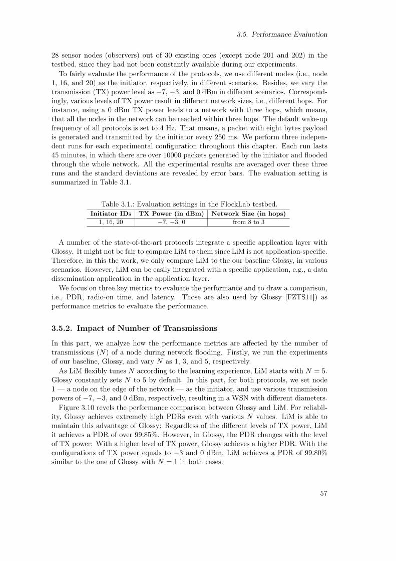
3.5. Performance Evaluation
28 sensor nodes (observers) out of 30 existing ones (except node 201 and 202) in thetestbed, since they had not been constantly available during our experiments.To fairly evaluate the performance of the protocols, we use different nodes (i.e., node
1, 16, and 20) as the initiator, respectively, in different scenarios. Besides, we vary thetransmission (TX) power level as −7, −3, and 0 dBm in different scenarios. Correspond-ingly, various levels of TX power result in different network sizes, i.e., different hops. Forinstance, using a 0 dBm TX power leads to a network with three hops, which means,that all the nodes in the network can be reached within three hops. The default wake-upfrequency of all protocols is set to 4 Hz. That means, a packet with eight bytes payloadis generated and transmitted by the initiator every 250 ms. We perform three indepen-dent runs for each experimental configuration throughout this chapter. Each run lasts45 minutes, in which there are over 10000 packets generated by the initiator and floodedthrough the whole network. All the experimental results are averaged over these threeruns and the standard deviations are revealed by error bars. The evaluation setting issummarized in Table 3.1.
Table 3.1.: Evaluation settings in the FlockLab testbed.Initiator IDs TX Power (in dBm) Network Size (in hops)
1, 16, 20 −7, −3, 0 from 8 to 3
A number of the state-of-the-art protocols integrate a specific application layer withGlossy. It might not be fair to compare LiM to them since LiM is not application-specific.Therefore, in this the work, we only compare LiM to the our baseline Glossy, in variousscenarios. However, LiM can be easily integrated with a specific application, e.g., a datadissemination application in the application layer.We focus on three key metrics to evaluate the performance and to draw a comparison,
i.e., PDR, radio-on time, and latency. Those are also used by Glossy [FZTS11]) asperformance metrics to evaluate the performance.
3.5.2. Impact of Number of Transmissions
In this part, we analyze how the performance metrics are affected by the number oftransmissions (N) of a node during network flooding. Firstly, we run the experimentsof our baseline, Glossy, and vary N as 1, 3, and 5, respectively.As LiM flexibly tunes N according to the learning experience, LiM starts with N = 5.
Glossy constantly sets N to 5 by default. In this part, for both protocols, we set node1 — a node on the edge of the network — as the initiator, and use various transmissionpowers of −7, −3, and 0 dBm, respectively, resulting in a WSN with different diameters.Figure 3.10 revels the performance comparison between Glossy and LiM. For reliabil-
ity, Glossy achieves extremely high PDRs even with various N values. LiM is able tomaintain this advantage of Glossy: Regardless of the different levels of TX power, LiMit achieves a PDR of over 99.85%. However, in Glossy, the PDR changes with the levelof TX power: With a higher level of TX power, Glossy achieves a higher PDR. With theconfigurations of TX power equals to −3 and 0 dBm, LiM achieves a PDR of 99.80%similar to the one of Glossy with N = 1 in both cases.
57

3. Machine Learning-based Flooding
0.9900.9920.9940.9960.9981.000
PDR
TX power = -7 dBmTX power = -3 dBmTX power = 0 dBm
02468
10Ra
dio-
on T
ime
(in m
s)
N = 1
N = 3
N = 5 LiM
N = 1
N = 3
N = 5 LiM
N = 1
N = 3
N = 5 LiM
0.00.51.01.52.02.5
Late
ncy
(in m
s)
Figure 3.10.: Performance metrics of Glossy with various N values and of LiM, respec-tively. Both protocols set node 1 as the initiator and use the transmissionpower of −7, −3, and 0 dBm. LiM inherits the advantages from Glossyin terms of high reliability with various levels of transmission power, whileeffectively reducing the radio-on time. The longer latency in LiM stemsfrom the overall processing time in the bandit learning phase.
Moreover, LiM succeeds in reducing unnecessary broadcast redundancy, resulting ina notable decreased portion of radio-on time, compared to Glossy with N = 3 and 5.The radio-on time is even close to the one of Glossy with N = 1 by using −3 or 0dBm as transmission power level. Even with a transmission power of −7 dBm, LiMis able to carry out a radio-on time similar to the one of Glossy with N = 3. Withthis configuration, the network might consist of 8 hops of nodes. As a side effect, thecommunication links in the network are more vulnerable because of a lower TX powerlevel, e.g., interference in the environment might influence the communications. In thisscenario, according to the radio-on time shown in the figure, we confirm, that LiMactively chooses the most conservative action — action 3 (N = 3) to maintain a reliableperformance.For the flooding latency, LiM does not perform better than Glossy in all three sce-
narios. This is because, that LiM has to spend more time for data processing, decisionmaking, and probability calculation, consequently leading to a latency of approximately2 ms in all cases. However, even with an end-to-end network latency of 2 ms, this couldstill meet a lot of mission-critical applications’ requirements.Please note, that in reality, Glossy with N = 1 may have a bootstrap problem and
experience a highly fragile network, according to our experience from the experiments
58

3.5. Performance Evaluation
that we carried out. We argue that LiM aims to interactively learn from the environ-ment and, thus, makes a decision of N to progressively reduce the broadcast redundancywhile maintaining acceptable levels of reliability, energy efficiency, and latency. In Sec-tion 3.5.4, we take a closer look at how LiM determines the number of transmissions(N).
3.5.3. Impact of Topology
In this section, we evaluate LiM with different positions of the initiator. We changethe position of the initiator (i.e., node 1, 16, and 20, respectively) to alter the floodingdiameter of the network, making the topology different in each set of experiments. Whilethe position of the initiator changes in the testbed, the network topology varies as well:Since the data source of a flooding changes, the absolute hop distance between a nodeand the source also changes. The idea of changing the position of the initiator is toevaluate whether a protocol is dependent on a specific topology or not. Besides, weexploit the transmission power of −7 dBm to result in a network with approximatelyeight hops.Figure 3.11 illustrates the results of LiM with various positions of the initiator (I),
i.e., positions of I are node 1, 16, and 20, respectively. For the reliability, LiM achievesa PDR of over 99.70% in all scenarios. The radio-on time and latency change slightlyalong with the position of the initiator. However, LiM maintains a less than 6 ms radio-on time and a less than 2 ms end-to-end latency only with a transmission power of −7dBm regardless of the initiator’s position.
I = 1
I = 16
I = 20
0.990
0.992
0.994
0.996
0.998
1.000
PDR
I = 1
I = 16
I = 20
0
1
2
3
4
5
6
7
Radi
o-on
Tim
e (in
ms)
I = 1
I = 16
I = 20
0.0
0.5
1.0
1.5
2.0
2.5
Late
ncy
(in m
s)
Figure 3.11.: Performance metrics of LiM with various initiator positions using a TXpower of −7 dBm. Even with relatively weak link connections, the net-work can still provide high reliability, low radio-on time, and low latency,regardless of the initiator’s position.
59

3. Machine Learning-based Flooding
3.5.4. Impact of Exploration Phase
In this part, we discuss the influences of the absorbing nodes and the reliability drop inthe exploration phase, respectively.
3.5.4.1. Absorbing Nodes
In general, the main part of redundancy reduction is contributed by the explorationphase in LiM, where the absorbing nodes are discovered. These absorbing nodes stayin a receiving mode and do not forward a received packet after waking up from thesleeping mode. Figure 3.12 shows the average number of each node in LiM from oneexperiment with node 1 as the initiator and 0 dBm transmission power. As the figuresshows, the absorbing nodes are successfully discovered in this case. The nodes thathave no transmission are actually the absorbing nodes, as the other nodes are the set ofbackbone nodes of the network.
1 2 3 4 6 7 8 10 11 13 14 15 16 170
1
2
3
4
18 19 20 22 23 24 25 26 27 28 31 32 33 2002040
1
2
3
4
Avera
ge N
um
ber
of
Tra
nsm
issi
ons
Node Index
Figure 3.12.: Average number of transmissions in each node with node 1 as the initiatorand 0 dBm TX power. The dotted line shows the overall average number oftransmissions. A node in LiM starts with N equal to 5 and progressivelydetermines N : The average value of N in each node is determined byitself. After the learning phase, LiM successfully finds all absorbing nodesand eventually obtains an average N equal to 1 as the dotted line shows.
3.5.4.2. Reliability Drop
A node in the exploration phase exploits a temporary “log-out” strategy, where it doesnot transmit a received packet for a flooding round, so as to review whether it is anabsorbing node. In this case, the network reliability cannot be guaranteed to be 100%.However, by default, LiM only reserves ten flooding rounds for each node to explore
60

3.5. Performance Evaluation
its role. Additionally, during these rounds, a node only logs out of the network for oneparticular round (out of 10), where the node only stays in receiving mode and does nottransmit. Consequently, assuming there are 30 nodes in a WSN and that nodes are wellsynchronized, then a node can lose 29 packets out of 300 (i.e., 10×30) in the worst case,i.e., PDR equals 90.33% (i.e., (300 − 29)/300). Figure 3.13 illustrates the dynamicallychanging PDRs of all the nodes in the testbed along with the running time. As shown,even though several nodes suffer a packet loss during the exploration phase, they arestill able to maintain a high reliability afterwards.
0 270 540 810 1080 1350 1620 1890 2160 2430 2700Run-time (in s)
0.90
0.92
0.94
0.96
0.98
1.00
PD
R
Node 2
Node 3
Node 4
Node 6
Node 7
Node 8
Node 10
Node 11
Node 13
Node 14
Node 15
Node 16
Node 17
Node 18
Node 19
Node 20
Node 22
Node 23
Node 24
Node 25
Node 26
Node 27
Node 28
Node 31
Node 32
Node 33
Node 200
Node 204
Figure 3.13.: PDRs of all nodes in FlockLab changing over run-time. PDR drops duringthe greedy exploration phase while finding all the absorbing nodes, butit is still higher than 90%. In this case, users can decide whether to putimportant or dummy data in the payload during the exploration phaseaccording to application-level requirements.
3.5.5. Discussion
To summarize, in this section, we demonstrated the performance of two different proto-cols: LiM and the baseline protocol Glossy, respectively, in various evaluation scenarios.The experimental results revealed that LiM effectively inherits the benefits from con-current transmission. It delivers a high end-to-end reliability of over 99.70% with anaverage end-to-end latency of less than 2.4 ms in all cases. More importantly, LiM isable to decrease the radio-on time to less than 6 ms step-by-step, and significantly re-duces broadcast redundancy. Even with different topologies, LiM is able to manage ahigh reliability with low end-to-end latency, while reducing unnecessary communicationredundancy. Table 3.2 shows the memory usage, i.e., Random-Access Memory (RAM)and Read-Only Memory (ROM), of LiM and Glossy, respectively, in Contiki OS 2.7.Even Equipped with a reinforcement learning scheme, LiM does not increase a lot of thememory usage compared to Glossy.
Table 3.2.: Memory usage of different protocols in Contiki OS 2.7.
Protocol Code Footprint (Kb)ROM RAM
LiM 22.554 0.526
Glossy 17.900 0.432
61

3. Machine Learning-based Flooding
Finally, Table 3.3 summarizes all the experimental results of different scenarios in thischapter. Please note, that we do not include the experiments of tuning the initiator’sposition for Glossy, since we focus on the self performance comparison of LiM in thischapter. For the interest of this part of Glossy, we refer the reader to the Glossy paper[FZTS11] and LWB paper [FZMT12].
3.6. Conclusion
This chapter introduces LiM, a machine learning-based flooding protocol for low-powerduty-cycled WSNs. LiM applies a multi-armed bandit learning scheme in CT-basedflooding, thereby benefiting from both. Concurrent transmissions ensure LiM a highlyreliable communication with low end-to-end latency and low energy cost. Machine learn-ing brings the adaptation ability to deal with the dynamics of the environment, therebyfurther improving energy efficiency. We implement our protocol in Contiki OS and eval-uate it with extensive experiments in a real-world testbed FlockLab. Our experimentalevaluation shows that LiM achieves less radio-on time, and — as a consequence — itgreatly improves energy efficiency of the network. Meanwhile, LiM manages a more than99.70% average end-to-end reliability and a less than 2.4 ms average end-to-end latencyin all experiments in the testbed. Furthermore, with its learning ability, LiM maintainsa flexible adaptation to the dynamics of the network, when compared to the baselineprotocol Glossy. To sum up, LiM inherits the benefits from concurrent transmissionsand a machine-learning scheme, outperforming the baseline protocol Glossy in the lightof energy efficiency while maintaining a high end-to-end reliability and low latency.
62

3.6. Conclusion
Tab
le3.3.:S
ummaryof
expe
rimentalresults.In
allexp
erim
entalscena
rios,L
iMmaintains
abe
st-effo
rten
d-to-end
PDRan
dlatenc
y,taking
advantag
eof
concurrent
tran
smission
s.Besides,LiM
decreasesap
proxim
ately
5msradio-on
timecompa
redto
thedefaultconfi
guration
ofGlossy.
The
max
imal
valueof
radio-on
timein
GlossyisN
=5,
while
theminim
umvalue
isN
=1.
LiM
redu
cestheradio-on
timeby
atleast3mscompa
redto
thede
faultsettingof
Glossy(i.e.,N
=5).
Protocol
InitiatorID
TX
Pow
erPDR
(%)
Rad
io-onTim
e(m
s)Laten
cy(m
s)
Glossy
Nod
e1
0dB
m99
.97
5.42
1.24
(max
:10
0.00
min:99
.88)
(max
:8.41
min:2.53
)(m
ax:1.26
min:1.23
)
-3dB
m99
.97
5.61
1.44
(max
:10
0.00
min:99
.88)
(max
:8.71
min:2.61
)(m
ax:1.69
min:1.30
)
-7dB
m99
.84
6.17
1.95
(max
:99
.97min:99
.66)
(max
:9.26
min:3.25
)(m
ax:2.03
min:1.89
)
LiM
Nod
e1
0dB
m99
.91
3.02
2.00
(max
:99
.98min:99
.80)
(max
:3.22
min:2.82
)(m
ax:2.12
min:1.92
)
-3dB
m99
.84
3.48
2.01
(max
:99
.92min:99
.76)
(max
:3.69
min:3.25
)(m
ax:2.34
min:1.44
)
-7dB
m99
.86
6.00
1.95
(max
:99
.95min:99
.73)
(max
:6.33
min:5.68
)(m
ax:2.33
min:1.62
)
Nod
e16
0dB
m99
.97
3.89
0.91
(max
:99
.99min:99
.94)
(max
:4.70
min:3.14
)(m
ax:1.06
min:0.80
)
-3dB
m99
.84
3.64
1.53
(max
:99
.91min:99
.76)
(max
:4.07
min:3.27
)(m
ax:1.58
min:1.48
)
-7dB
m99
.89
4.87
1.28
(max
:99
.96min:99
.84)
(max
:5.38
min:4.34
)(m
ax:1.38
min:1.18
)
Nod
e20
0dB
m99
.91
2.96
0.94
(max
:10
0.00
min:99
.79)
(max
:3.11
min:2.83
)(m
ax:1.12
min:0.87
)
-3dB
m99
.93
3.11
1.18
(max
:99
.94min:99
.92)
(max
:3.20
min:2.98
)(m
ax:1.23
min:1.07
)
-7dB
m99
.95
4.47
1.40
(max
:99
.98min:99
.92)
(max
:4.77
min:4.18
)(m
ax:1.44
min:1.35
)
63


4Concurrent Transmission-based
Collection
4.1. Introduction
In smart city scenarios, hundreds or thousands of distributed battery-powered sensornodes communicate wirelessly over single or multiple hops. These nodes cooperate to-gether in order to fulfill various tasks and to provide an acceptable level of QoS to theusers. However, owing to the resource-constrained nature of sensor nodes, providingsatisfactory application-level QoS in WSNs is extremely challenging, especially in multi-hop, low-power, and lossy networks. For instance, mission-critical applications — suchas data collection in smart grids — usually require not only high energy efficiency andhigh reliability but also ultra low latency.Rising as a novel communication paradigm, Concurrent Transmission (CT) is intro-
duced by Ferrari et al. [FZTS11]. As the first CT-based flooding primitive, Glossy[FZTS11] has caught much attention in the community. By exploiting a receive-and-forward scheme, sensor nodes transmit an identical packet at the same moment (e.g.,within 0.5 µs) to achieve a constructive interference and the capture effect [FZTS11].It has proven, that CT allows messages to be propagated in the whole network in sev-eral milliseconds without any severe collisions. Glossy achieves energy-efficient floodingwithout causing broadcast storm problems and, thus, does not require any routing infor-mation in the network. Basically, Glossy is based on an accurate time synchronization torealize CT. In this respect, it differs from the Carrier Sense Multiple Access with Colli-sion Avoidance (CSMA/CA)-based IEEE 802.15.4 standard, e.g., used by IPv6 RoutingProtocol for Low-Power and Lossy Networks (RPL) [Win12].
65

4. Concurrent Transmission-based Collection
Data collection, as a many-to-one scenario, is one of the most important WSN-basedapplications. This scenario requires that sensor nodes (also referred to as source node),where the data are generated, e.g., temperature, humidity, vibration, and rotation, trans-mit the data packets to a so-called sink (node). Acting as a central base station, thesink collects and processes all the data packets from the sensor nodes throughout thenetwork, so as to fulfill the data collection tasks. The state-of-the-art collection proto-cols, such as CTP [GFJ+09], RPL [Win12], Opportunistic Routing for Wireless sensornetworks (ORW) [LGDJ12], Opportunistic RPL (ORPL) [DLV13], and MOR [ZLT17]stick to CSMA/CA to deal with collisions. Inevitably, the back-off scheme of the CS-MA/CA approach introduces longer latency and the re-transmission introduces higheroverhead. In contrast, CT-based data collection has the potential of effectively providinghigh end-to-end reliability and low latency. This is, because CT-based protocols do notrequire MAC-layer collision avoidance and network-layer routing, as presented in theLWB [FZMT12] and Chaos [LFZ13a], since CT replies on constructive interference andthe capture effect. In other words, CT counts on collisions but the constructive ones,which come from the tight time synchronization and the identical packet through thewhole network in a flooding round.Nevertheless, current CT-based protocols used for data collection have to deal with two
main issues: (i) a flooding-based communication primitive and (ii) network-level schedul-ing. This type of communication primitive requires that the packet must be identicalin one flooding period within the whole network, so that constructive interference canfunction. Besides, the capture effect is exploited to correctly receive a packet with thestronger signal strength, when multiple senders are concurrently transmitting [LFZ13a].As a consequence, certain source nodes can never successfully transmit their packets tothe receiver if they are not well scheduled globally. Even worse, when too many nodesconcurrently transmit different packets, then the destructive collision occurs more often.That leads to a decreasing PDR, a broken flooding process, and clock desynchronizations.To address this problem, Ferrari et al. [FZMT12] designed an application-level schedul-
ing mechanism for multiple source nodes by a dedicated host in the network. The hostcentrally computes a schedule and periodically distributes the schedule to all nodes inthe network to coordinate the traffic. This technique, however, inevitably introduces acollision period in the beginning of network initialization to construct a global schedulerin a many-to-one communication pattern. Moreover, LWB [FZMT12] triggers periodicalsynchronization with identical packets in the network to accurately achieve global syn-chronization. Consequently, the schedule-based many-to-one communication approachincreases the complexity of the CT-based network. We argue that there could be atechnique to achieve CT-based data collection without any scheduler. We propose anew communication primitive — Packet-in-Packet (PiP) — for timely and reliable datacollection in multihop low-power WSNs.PiP uses concurrent transmissions, i.e., constructive interference and the capture ef-
fect, to inherit the advantages: high reliability, low latency, and low energy consumption.PiP is able to grant accurate clock synchronization even with different packets in thenetwork. Moreover, PiP exploits packet concatenation to achieve concurrent data col-lection from multiple neighboring nodes in a single Transmit (TX) slot. By nature, PiPconcatenates multiple packets from neighboring nodes in the air. Therefore, it requiresneither a global scheduler nor a dedicated setup period. From the network perspective,
66
4.2. Related Work
PiP coordinates the concatenated packet that contains multiple packets from varioussource nodes as a “higher-priority” packet to the sink. As a result, PiP reduces datacollection time and maintains high reliability and high energy efficiency compared to thestate-of-the-art.The remainder of this chapter is organized as follows. Section 4.2 discusses related
work, with foci on CT-based protocols and packets in a packet in low-power wirelessnetworks. Section 4.3 explains the basics of our proposed protocol and provides a briefoverview. Section 4.4 details the design of PiP, followed by a performance evaluation inSection 4.5. Section 4.6 provides concluding remarks.
4.2. Related Work
In this section, we review a number of existing research work in terms of CT-based pro-tocols in WSNs and the concept of “packets in a packet” in WSNs. Next, we summarizethe related work.
4.2.1. CT-based Protocols
Network flooding is one of the most fundamental services in WSNs. It forms the basis fora wide range of applications and network operations. Glossy [FZTS11] provides a fastand efficient network flooding service by using concurrent transmissions in WSNs. Byexploiting constructive interference and the capture effect on the physical layer, Glossyis able to get an average packet delivery ratio of 99.99% and ultra-low latency in realtestbeds.Splash [DCL13] builds a tree pipeline [RCBG10] by exploiting Glossy, thereby improv-
ing channel utilization. Furthermore, Pando [DLZL15] integrates fountain code [Mac05](also known as rateless erasure codes) with pipelining to further improve the reliabilityof Splash. While Glossy disseminates one packet in each communication round, Splashand Pando are designed to deliver large data objects to all nodes in a WSN, e.g., forthe purpose of reprogramming or firmware update the WSN-based applications. Rip-ple [YH15] also relies on Splash and network coding techniques to improve particularlyin terms of network throughput.However, Glossy aims to provide highly reliable flooding for one-to-many applications.
Thus, it is not applicable for many-to-one applications such as data collection. To realizethe design of many-to-one applications with Glossy, Ferrari et al. added an application-level scheduler to construct a so-called Low-power Wireless Bus (LWB) [FZMT12]. LWBcentrally schedules the data communication to support one-to-many, many-to-one, andmany-to-many traffic patterns in WSNs. Moreover, Chaos [LFZ13a] builds on Glossy toachieve fast all-to-all data sharing in a distributed manner. Chaos further combines pro-grammable in-network processing with concurrent transmissions in WSNs. Meanwhile,Suzuki et al. proposed a reliable data collection protocol based on Glossy for many-to-one applications named Choco [SYM13]. By their testbed evaluations, they arguedthat Choco can provide more energy-efficient collections than the state-of-the-art andachieves high end-to-end reliability.Apart from aforementioned protocols, there are a number of efforts to construct one-
to-one application on Glossy. For instance, Carlson et al. propose CXFS [CCT+13], a
67

4. Concurrent Transmission-based Collection
forwarder selection mechanism for concurrent transmissions. In CXFS, sensor nodes usea hop count in each packet to get their relative distance to each other. CXFS builds onGlossy and supports point-to-point transmissions while achieving high reliability, highenergy efficiency, and high throughput. Moreover, Sparkle [YRH14] selects subsets ofnodes that participate in Glossy-based flooding. It also supports one-to-one communi-cation. Similarly, RTF [ZRHK15] further extends Sparkle and exploits TDMA for datascheduling to improve reliability and energy efficiency in point-to-point traffic. RFTidentifies reliable relay nodes to limit the number of concurrently active neighbors tosave more energy. More recently, LaneFlood [BLS16] builds on Glossy and further inte-grates the forwarder selection scheme of CXFS with application-level network protocolsin WSNs. LaneFlood thus supports one-to-one traffic, forwarder selection, and standardprotocols in IoT such as TCP/UDP and the constrained application protocol (CoAP)— a specialized Internet Application Protocol for constrained devices, as defined inRFC7252 [She14].
4.2.2. Packets in a Packet
Santhapuri et al. investigated link-layer opportunities and challenges towards harness-ing the feature of a so-called message-in-message (MIM) in [SCM+08]. They proposedan MIM-aware framework that reorders transmissions to enable concurrent communica-tions. By continuously scanning for sync-words, their technique allows a transceiver todisengage from the reception of an ongoing transmission and to lock onto a newly-startedstronger one.
The usage of in-band signaling to denote the start of a packet is almost universal indigital radios. Authors in [GBM+11] demonstrate that by exploiting this this property,in-band radio signaling mechanisms can be abused to inject raw digital frames. Fromthe perspective of security, they provide a few tested examples of raw frame injectionfor digital radios such as IEEE 802.15.4 radio. Besides, they show that an attacker caninject frames into a packet, if he/she is able to predict the on-air pattern produced byencapsulated data.
More recently, König et al. [KW16] proposed a class of wireless transmission schemesthat decouple synchronization headers from payloads in order to create new transmissionprimitives of a second sender. By only transmitting a synchronization header, a nodeis able to let the neighboring nodes receive fragments of a packet. Besides, portionsof the payload of longer ongoing packets can be overwritten by exploiting the captureeffect. The authors then explored two scenarios potentially benefiting from such schemes:crossing a network “chasm” (i.e., a virtual or physical gap between two parts of thenetwork where communication links are very poor) and insertion of high-priority packets.Further, they examined the technique in these two scenarios. Results in testbeds showedthat the packet-received ratio can be increased from 5% to up to 30% in the case ofnetwork chasm. In the second scenario, the successful decoding of the injected packet inup to 70% of the cases could be reached.
68

4.3. Overview
4.2.3. Summary
Over the years, CT has been proven to be an efficient approach to improve the timelinessand reliability, because packets can positively overlap rather than collide in the air.CT is able to achieve good performance for one-to-many scenarios due to the naturalproperty of flooding. For many-to-one scenarios — e.g., data collection, the most popularapplications of a WSN — CT can be only implemented with additional scheduling orcontent compression on the application layer. However, for the applications requiringoriginal data in a dynamic network, scheduling in advance and content compressionsometimes hardly work. PiP, on the contrary, is suitable for this type of scenarios.Original data collection is supported by PiP without any scheduling or compression. Sofar, to the best of our knowledge, there is no application working in the manner as PiPdoes in practice.
4.3. Overview
In this section, we explain the prerequisites of concurrent transmission in low-powerWSNs — constructive interference and the capture effect. Then, we briefly introducethe concept and background of LiM. Last, we give a general review of PiP.
4.3.1. Concurrent Transmission
Glossy [FZTS11] has boosted much new research interest in wireless network communi-ties, as one of the most representative CT-based flooding protocols in the community.Generally, it exploits constructive interference and the capture effect: It uses construc-tive interference to superimpose (identical) packets; and it exploits the capture effectto ensure, that a receiver successfully receives a packet and correctly demodulates thepacket while multiple senders simultaneously transmitting. Using these two mechanisms,Glossy is able to manage a highly reliable flooding and an accurate time synchroniza-tion [FZTS11].In Glossy, nodes in the network get time-synchronized to a so-called “initiator” —
from which the data flooding is initiated — in order to estimate the time to wake upand listen to the channel. Moreover, nodes concurrently transmit packets in a “receive-and-forward” scheme, which means whenever a node receives a valid packet, then itimmediately forwards the packet to all the neighboring nodes. In this way, messages arepropagated through the network without contention of the wireless medium. To someextend, Glossy makes use of contention due to the nature of constructive interferenceand the capture effect. Ferrari et al. [FZTS11] argue, that the latency of flooding couldapproximately reach the theoretical upper bound since every node in the network is ina receive-and-forward manner to spread the messages. The manner introduces no extraoverhead in terms of time as the traditional CSMA/CA does, e.g., the back-off time forcontention avoidance.Constructive interference occurs only when two or more nodes transmit identical pack-
ets. With IEEE 802.15.4 radios operating in the 2.4 GHz ISM band, these identicalpackets are required to overlap within 0.5 µs [FZTS11,DDHC+10]. This enables makesthe packets appropriately superimposed, thereby, can be correctly received and demod-
69

4. Concurrent Transmission-based Collection
ulated by the receiver. The capture effect is a phenomenon, where the receiver can lockonto and correctly demodulate a packet, when the signal of the packet is approximately3 – 4 dB stronger than the sum of all the other signals [LF76,FZTS11]. Besides, in IEEE802.15.4 radios, the strongest signal must arrive no later than 160 µs after the weakersignals [LFZ13a], in order to be properly recognized and decoded by the receiver. Formore details of CT, i.e. constructive interference and the capture effect, we refer thereader to Section 3.3.1 in Chapter 3.
4.3.2. Packets in a Packet
Technically, most wireless receivers — including IEEE 802.15.4 radios — start to record apacket in the air once a synchronization header (i.e. preamble is detected. They stop therecording based on the frame-length byte in the packet [Tex06]. However, if a collisionoccurs during the reception of synchronization header, then nothing can be received bythe radio. In other words, if a synchronization header of a data frame (i.e. packet) iscaptured by a radio, then the radio can be synchronized with the data frame. It thenrecords for the time of a frame with the length of the value written in the frame-lengthbyte. Some related work concentrates on empowering the radios to avoid medium accesscollisions and to receive more valid bytes. However, König et al. [KW16] recently proposea class of wireless transmission primitives by investigating on collisions, specifically, thecapture effect. This primitive decouples synchronization headers from payloads in orderto create new transmission primitives of a second sender. By using the capture effect,different neighboring senders can overwrite portions of the payload in ongoing packetsin the air.
4.3.3. PiP in a Nutshell
Motivated by König et al. [KW16], we propose a link-layer communication primitive —PiP— that by nature manages the “in-packet” time slots for various neighbors in a singletransmission. On the one hand, PiP is similar to TDMA scheme: It builds on CT anddivides a transmission into several time slots. In PiP, this kind of time slot is defined as“in-packet” slot, which is further explained later in Section 4.4.2.2. On the other hand,different from other power control-based approaches, PiP relies on a hardware-based PAoperation. Namely, a PA is an electronic amplifier that converts a low-power RF signalinto a higher-power RF signal. This means, if being switched off, a PA can be then usedto lower the power level of the output RF signals of the radio. PiP relies on this typeof operation during transmission: While multiple neighboring senders are concurrentlytransmitting to a single receiver, one or more of them can give away the opportunitiesto others that are simultaneously transmitting. As a result, PiP is able to successfully“control” the capture effect in presence of multiple senders, so that every sender canfairly transmit the packet to the receiver instead of being negatively “captured” (i.e.,cause a collision). Moreover, PiP requires no global scheduling and causes no extraoverhead of routing. Meanwhile, it achieves accurate time synchronization inheritedfrom Glossy [FZMT12], even when the content of packets is different the network. In aword, by realizing packet-in-packet, PiP is able to obtain timely, reliable, and energy-efficient data collection in multihop low-power WSNs.
70

4.4. Design of PiP
4.4. Design of PiP
In this section, we detail the design aspects of PiP. We discuss the basis of PiP: con-current transmission and the packet concatenation scheme, respectively. Moreover, wedepict the network-wide data collection with PiP and additional implementation aspectsin detail.
4.4.1. Concurrent Transmission-based Collection
PiP is based on concurrent transmissions, i.e., constructive interference and the captureeffect, as derived from the essence of Glossy [FZTS11]. In general, PiP is a sink-initiateddata collection protocol, since CT-based data collections are always triggered by the sink.In a data collection phase, there are typically various packets generated by differentsensor nodes throughout the network. The content of these packets are most oftendifferent in a collection round. For instance, in a machine data collection scenario,various sensors can measure different values from the physical world, e.g., vibrationsfrom different machines. Correspondingly, constructive interference may not functioneffectively. The capture effect, in this case, however, enables the receiver to correctlyreceive a packet with the stronger received signal strength if all the senders are highlysynchronized (i.e., the time difference is less than 160 µs).Generally, to well handle data collection, CT protocols exploit either global scheduling
such as LWB [FZMT12] or real-time in-network processing such as Chaos [LFZ13a]. Thekey foundation of CT protocols is one-to-all data flooding, which makes all-to-one datacollection rather challenging, because the data flows are totally different. Moreover, CTsrequire highly accurate time synchronization between senders and the identical contentof packets throughout the network.PiP manages time synchronization with network flooding (similar to Glossy), while
employing a number of in-packet slots to collect the data from the single-hop neighborsin a single transmission round. In other words, PiP uses one-to-all data flooding tomaintain accurate time synchronization and utilizes various minor slots within a packetto achieve all-to-one data collection. When dealing with the capture effect, PiP doesnot manipulate power control as other approaches do, e.g., tuning the TX power level ofthe radio. Instead, PiP relies on a type of hardware-based operation — a so-called PAoperation.Figure 4.1 reveals the basic idea of the packet concatenation with a network of five
nodes, where node H is the sink node that ought to collect the data packets from allthe neighboring nodes. In time slot 0, node H broadcasts a packet to all the neighbor-ing nodes, so as to maintain the accurate synchronizations (similar to Glossy). Afterthe neighboring nodes have received the packet, they concurrently transmit their ownpackets immediately in the following time slot, i.e., time slot 1 in Figure 4.1. Thisreceive-and-forward pattern is inherited from CTs, which helps in keeping accurate timesynchronization throughout the network. In time slot 1, every transmitter has its owncorresponding time period (i.e., defined as in-packet slot in PiP) to transmit its ownpacket (i.e., defined as in-packet packet in PiP).A single transmitter only switches its PA on when it is its turn to transmit. For
instance, node A switches PA off after it finishes transmitting its in-packet packet in the
71

4. Concurrent Transmission-based Collection
corresponding in-packet slot. Then, node B switches its PA on and starts to transmit itsown in-packet packet. As a result, using the PA operation, multiple senders in PiP areable to transmit their own in-packet packets in different (minor) slots of one major timeslot, as shown in the figure. At the receiver (node H), different in-packet packets arenaturally concatenated in the air and formed as a longer packet afterwards. Please note,that PA operation is different from radio-on and -off operations. That is, switchingPA on and off does not mean powering the radio on and off; Instead, PA operationcan only be done when the RF radio is powered on. In the following, we explain thetransmission process and the PA operation based on one of the IEEE 802.15.4 radios —CC2420 [Ins07], respectively.
A
B
H
C
D
TX
B
Time Slot 0 1
RX
TX RX
Transmission Reception
In-packet packet
Concurrent transmission
Radio-on period
RX
RX
RX
RX
TX
TX
TX
TXA
C
D
A B C D
...
...
...
...
...
...
In-packet slot
Figure 4.1.: Single-hop packet concatenation in PiP. Node H collects data packets fromneighboring nodes in a single transmission round. Node H manages timesynchronization by flooding and collects various data packets in differentminor time slots of a major receiving time slot.
Furthermore, in the extent of a network, basically, the whole process of data collectionin PiP can be defined as a PiP period. Each PiP period consists of a number of PiProunds. Subsequently, each PiP round is made up of several CT slots. One CT slot isfor the transmission or the reception of one single PiP packet. We provide more detailsin Section 4.4.3: How PiP works in the scope of a multihop low-power WSN.
4.4.1.1. Radio Frequency Transmission
A radio frequency power amplifier (PA) is a type of electronic amplifier that enhancesthe power of radio-frequency signal. For a better explanation, the RF transmission ofCC2420 radio is briefly explained in this section.
On a CC2420 radio chip [Ins07], each byte to be transmitted in TX First In First Out(FIFO) buffer is divided into two symbols, of four bits each. Each symbol is spread bythe IEEE 802.15.4 spreading sequence to 32 chips. Then, the chips are converted by theDigital-to-Analog Converter (DAC). Afterwards, the low pass filter and the quadratureup-conversion mixers convert the modulated analog baseband signals (I and Q) to RFsignals on the given channel. Finally, the RF signals are amplified by PA based on the
72

4.4. Design of PiP
PA_LEVEL in the TXCTRL register [Ins07]. Then, they are fed to the antenna ports(RF Input/Output (I/O)). For more details of CC2420 transmission procedure, we referthe readers to the manual of CC2420 from Texas Instruments [Ins07]. Note, that RFsignals could be fed to the RF I/O directly, without PA amplification, but the power ofelectromagnetic radiation would be quite limited. Consequently, if the signals are fed tothe RF I/O directly (without PA amplification), then even a receiver that is extremelyclose to a sender may detect nothing in the air. In this work, we exploit this phenomenonto enable packet concatenation in PiP without tuning TX power level.
4.4.1.2. Power Amplifier Operation
Generally, a RF PA is a type of electronic amplifier that converts a low-power RF signalinto a higher-power signal, as shown in Figure 4.2 [Tex06]. Typically, the RF signal isamplified in the PA, fed to the antenna and then transmitted in the air. In our research,we explore that it is feasible to manipulate PA when a packet is being transmitted.PA can be switched on and off via the registers MANAND and MANOR in CC2420radio [Ins07] during the transmission. Hence, a packet in PiP can be virtually consideredas a number of PA-on and PA-off in-packet packets. Later in this section, we detail theframe structure in PiP. The sender in PiP switches its PA on if it intends to transmit aown packet, and switches PA off while there is nothing to transmit. Besides, the receiverreceives the concatenated packet in the air by nature without any PA operation.
CC2420
SWRS041c Page 17 of 85
8 Circuit Description
Seri
al
mic
roco
ntr
oller
inte
rfa
ce
LNA
DIGITAL
DEMODULATOR
- Digital RSSI
- Gain Control
- Image Suppression
- Channel Filtering
- Demodulation
- Frame
synchronization
DIGITAL
MODULATOR
- Data spreading
- Modulation
On-chip
BIAS
DIGITAL
INTERFACE
WITH FIFO
BUFFERS,
CRC AND
ENCRYPTION
CO
NT
RO
L L
OG
IC
AUTOMATIC GAIN CONTROL
TX POWER CONTROL
TX/RX CONTROL
XOSC
16 MHz
R
ADC
ADC
DAC
DAC
0
90
FREQ
SYNTH
SmartRF
CC2420
Power
Control
PA
Serial
voltage
regulator
Digital and
Analog test
interface
Figure 2. CC2420 simplified block diagram
A simplified block diagram of CC2420 is shown in Figure 2.
CC2420 features a low-IF receiver. The received RF signal is amplified by the low-noise amplifier (LNA) and down-converted in quadrature (I and Q) to the intermediate frequency (IF). At IF (2 MHz), the complex I/Q signal is filtered and amplified, and then digitized by the ADCs. Automatic gain control, final channel filtering, de-spreading, symbol correlation and byte synchronisation are performed digitally.
When the SFD pin goes active, this
indicates that a start of frame delimiter has
been detected. CC2420 buffers the received data in a 128 byte receive FIFO. The user may read the FIFO through an SPI interface. CRC is verified in hardware. RSSI and correlation values are appended to the frame. CCA is available on a pin in receive mode. Serial (unbuffered) data modes are also available for test purposes.
The CC2420 transmitter is based on direct up-conversion. The data is buffered in a 128 byte transmit FIFO (separate from the receive FIFO). The preamble and start of frame delimiter are generated by hardware. Each symbol (4 bits) is spread using the IEEE 802.15.4 spreading sequence to 32 chips and output to the digital-to-analog converters (DACs).
An analog low pass filter passes the signal to the quadrature (I and Q) upconversion mixers. The RF signal is amplified in the power amplifier (PA) and fed to the antenna.
The internal T/R switch circuitry makes the antenna interface and matching easy. The RF connection is differential. A balun may be used for single-ended antennas. The biasing of the PA and LNA is done by connecting TXRX_SWITCH to RF_P and
RF_N through an external DC path.
The frequency synthesizer includes a completely on-chip LC VCO and a 90
Not Recommended For New Designs
Figure 4.2.: Functional diagram of IEEE 802.15.4 radio CC2420 on page 8 of the techni-cal datasheet [Tex06]. Power amplifier (PA) is located in the lower left sidein the figure.
Moreover, the PA operation in PiP also offers another benefit: less energy overhead.For low-power WSNs, the energy consumption is always one of the most critical issues. InPiP, when a node switches PA off, the energy consumption can be significantly reduced.
73

4. Concurrent Transmission-based Collection
Figure 4.3 illustrates one specific case of a TelosB sky mote with 0 dBm TX power. Withthe setting of 0 dBm TX power, the radio normally consumes around 28 mA currentfor transmission, as the figure shows. With PA operation, specifically switching PA off,the radio saves approximately 10 mA current for almost half a period. When switchingthe PA on, the radio costs the same current consumption as the one without any PAoperation.
0 200 400 600 800 1000 1200 1400Samples
5
10
15
20
25
30Cu
rrent
(mA)
Without PA operationWith PA operation
Figure 4.3.: Energy cost of IEEE 802.15.4 radio (CC2420) with and without PA opera-tion at TX power level of 0 dBm.
Please note, that the current consumption in Figure 4.3 includes all overheads such asthe energy consumed by the micro-controller, light and temperature sensors, and radiotransceiver. In this case, this leads to a higher current level than the one in the CC2420datasheet [Tex06], i.e. 17.4 mA at 0 dBm TX power. As the zoomed-in sub-figureshows, the current drops deeper when the node switches PA off (in blue) compared tothe one without PA operation (in red). This implies, that PiP can benefit from the PAoperation in terms of energy consumption. According to our experimental measurements,we calculate that the current consumption is approximately 6.1 mA when PA is switchedoff. For the sake of simplicity, we calculate the energy consumption of the CC2420 radioaccording to Equation 4.1.
ETXwithPA∝ (EPA_ON +
EPA_OFF
ω) (4.1)
where ETXwithPAis the energy consumption of a transmission with PA operation.
EPA_ON and EPA_OFF are the energy consumption when PA is turned on and off,respectively. For a fair comparison to other protocols, we use ω, a factor convertingthe current consumption with PA operation to an overall one provided in the datasheet[Tex06], in order to compute the average energy consumption of PiP. Furthermore, thecorresponding current consumption [Tex06] with their factors at different TX powerlevels are summarized in Table 4.1.
74

4.4. Design of PiP
Table 4.1.: Current consumption mappings to the corresponding TX power levels[Tex06].
TX Power (dBm) Current Consumption (mA) ω
0 17.4 2.85-1 16.5 2.70-3 15.2 2.49-5 13.9 2.28-7 12.5 2.05-10 11.2 1.84-15 9.9 1.62-25 8.5 1.39
4.4.1.3. Concurrent Transmission with Power Amplifier Operation
We develop PiP with PA operation through (i) extending the packet length and (ii)dividing the extended packet into a number of in-packet slots. As a consequence, diverseinformation from multiple single-hop nodes can be received successfully as long as thevarious in-packet parts do not overlap in the concatenated packet. Based on CT withPA operations, PiP can realize the single-hop packet concatenations.
4.4.2. Packet Concatenation
In this section, we address the following three key aspects to make PiP working. First,the frame structure in PiP is elaborately re-designed since the received packet cannotbe validated automatically by the hardware. Besides, the flooding process with respectto transmission and synchronization should continue even when the in-packet packetscollide with each other. Moreover, the strategy to avoid overlapping is required to ensurethat most of the in-packet packets are tightly aligned and received correctly.
4.4.2.1. Frame Structure
To support the concatenation of packets in a packet, PiP extends the frame structure ofGlossy by adding a two-byte checksum field, a 10-byte bitmap for ACK and one dummybyte, as illustrated in Figure 4.4. The checksum is used to check the correctness ofthe parts, including the bytes of frame length, header, sequence number, relay counter,and bitmap of the concatenated packet. Besides, the dummy byte is considered as areserved period of time for parsing the received packet at the end of the transmission.The details of the PiP frame structure are shown in Figure 4.4. The PiP payload isdivided by a guard byte into various in-packet slots. The guard byte distinguishes thedifferent in-packet slots and reserves the time for operating the PA. In this case, thisbyte ensures that the PA operation does not affect the completeness of receiving eachindividual in-packet packet. Each in-packet slot (or packet) is assigned for each neigh-boring node correspondingly. Namely, an in-packet packet includes a one-byte header,a seven-byte payload, and a slot checksum. The slot checksum ensures the correctnessof the corresponding in-packet packet, so that every in-packet packet is independent ofeach other, even if an error occurs in the overall frame.
75

4. Concurrent Transmission-based Collection
In-packet Slot 2(9 bytes)
In-packet Slot 7(9 bytes)...Guard Byte
(1 byte)Guard Byte
(1 byte)Guard Byte
(1 byte)In-packet Slot 1
(9 bytes)
PiP Header(1 byte)
Sequence Number(4 bytes)
Relay Counter(1 byte)
Bitmap(10 bytes)
Checksum(2 bytes)
Payload(70 bytes)
Dummy(1 byte)
Payload (89 bytes)
Slot Header(1 byte) Payload (7 bytes) Slot Checksum
(1 bytes)
PiP Payload
In-packetSlot Frame
Preamble + SFD(5 bytes)
Footer(2 bytes)
Length(1 byte)
PHY-layer Frame
PiP Frame
Figure 4.4.: Hierarchical frame structure in PiP. PHY-layer frame refers to the physical-layer frame structure in IEEE 802.15.4 standard.
4.4.2.2. Concatenation in a Packet
In PiP, we divide one packet into a certain number of in-packet packets (e.g., into sevenin-packet packets) with fixed length. Correspondingly, the sender switches PA on whenthere is an in-packet packet to transmit and switches it off when there is nothing totransmit. The receiver detects the (identical) overlapped headers (i.e., the preamble andthe Start of Frame Delimiter (SFD)) from multiple senders because of CTs. As long asthere is one sender, which turns PA on during the in-packet slot, the receiver can receivethe corresponding PA-on parts successfully.As shown in Figure 4.5, two senders concurrently transmit their own information. The
receiver starts to record symbols in the air once a header is detected and stops basedon the frame-length byte, i.e., the first byte after the header. In a normal case of CT,when the content of two packets is identical, the receiver can correctly receive the packetdue to constructive interference. In this case, the first six bytes (i.e., the header and thelength) are received based on constructive interference. Otherwise, when the content isnot the same, the receiver can receive the packet with the higher power because of thecapture effect. In the case of PiP, the capture effect still happens if multiple sendersswitch PA on at the same time, e.g., in in-packet slot 4.
However, by switching the PA off, a sender in PiP is able to give away the opportunityof being received to the other senders. For instance, the receiver in Figure 4.5 receivesthe in-packet packet from sender 1 since sender 2 turns PA off in in-packet slot 1. Whenit comes to a special case (e.g., in in-packet slot 5), where two senders, both, turn PA off,the receiver does not detect anything in the air. However, in this case, the receiver stillmakes a soft decision (see the CC2420 manual [Tex06]), even though there is nothing inthe air. As a result, a random sequence is placed as the content of the PA-off part atthe receiver, as illustrated in in-packet 5.
Moreover, when the PA-off part passes and a following PA-on part arrives, then the PA-on part can be received and demodulated correctly because of the individual checksumin each in-packet slot (see in-packet slot frame in Figure 4.4). In this case, the receivedCRC in the footer is meaningless for the receiver since a random sequence might exist inthe packet. As a result, a received packet in PiP is validated by a software-based checkat the receiver instead of a hardware-enabled CRC.
76

4.4. Design of PiP
Generally, PiP maintains two schemes to concatenate in-packet packets (also referredto as packet injection): (i) packet injection with pre-reservation and (ii) random packetinjection. On the one hand, packet injection with pre-reservation refers that senders havetheir pre-defined transmission sequence for their own in-packet packet — pre-reseveredin-packet time slot. Therefore, the “collision” — where the capture effect occurs, e.g., inin-packet slot 4 shown in Figure 4.5 — can be avoided. Because this in-packet time slotcan either be assigned to sender 1 or sender 2.
In the single-hop scenario shown in Figure 4.1, neighbors of node H concurrently trans-mit the packet once they have been initiated by node H. Practically, there is almost nochance to pre-assign the in-packet slots for all nodes in a WSN. Compared to the afore-mentioned relatively “static” packet concatenation scheme, random (packet) injection,on the other hand, is more flexible that requires no knowledge of the network in advance,e.g., topology information. It enables senders to determine whether to transmit theirin-packet packet randomly in one in-packet slot without any pre-assigned transmissionsequence. Therefore, the node is allowed to transmit its in-packet packet in a randomlychosen in-packet slot, i.e., randomly injecting in-packet packet in the current in-packetslot.
To some extent, this randomness introduces the probability of collisions betweensenders, e.g., in in-packet slot 4 depicted in Figure 4.5. The capture effect would hap-pen only when multiple neighbors inject their different in-packet packets exactly intothe same in-packet slot. In this case, due to the capture effect, the receiver could onlyreceive the packet from one specific sender and would not receive the packets from otherneighboring nodes. In Section 4.5.2.2 and Section 4.5.2.3, we evaluate the performanceof both, PiP with pre-reservation and random injection, in terms of single-hop and mul-tihop scenarios, respectively.
Footer
In-packet packet 1
In-packet packet 2
In-packet packet 3
Footer
Footer
...
In-packet packet 4Preamble + SFD Length
Length
Random Sequence
In-packet packet 2
In-packet packet 4
In-packet packet 5
In-packet packet 1
In-packet packet 3
In-packet packet 5
Preamble + SFD In-packet packet 1
In-packet packet 3
Preamble + SFD In-packet packet 2
In-packet packet 4
Length
Preamble + SFD FooterLength PayloadIEEE 802.15.4Frame
Sender 1
Sender 2
Receiver 1
5 bytes 1 byte 2 bytes0 - 125 bytes
...
...
From Sender 1 From Sender 2 From Sender 1 Capture EffectConstructive Interference From the air Capture Effect
PA On PA Off Constructive InterferenceCapture Effect Soft decision
In-packet Slot 1 In-packet Slot 2 In-packet Slot 3 In-packet Slot 4 In-packet Slot 5 ...
Figure 4.5.: Packet concatenation of two senders with one receiver. Both senders switchPA on and off to ensure that the receiver is able to receive various in-packetpackets from all senders during one transmission slot. If both of two sendersturn PA off, then the receiver makes a soft decision according to [Tex06],thereby, placing a random sequence in the corresponding part.
77

4. Concurrent Transmission-based Collection
4.4.2.3. Time Synchronization
In this section, we explain how PiP exploits the designed frame structure to achieve timesynchronization. Most of the CT-based protocols achieve accurate time synchronizationby the receive-and-forward communication pattern proposed in Glossy [FZTS11]. Theaccurate time synchronization is based on identical packets in the whole network of asingle CT round. However, in PiP, the packets cannot be identical throughout the net-work due to the “collection” nature. Therefore, we deliberately design the PiP framestructure and use one part of the frame to realize time synchronization. More precisely,this part can be regarded as the CT-based in-packet packet, which is identical throughthe network. Namely, it refers to the first 24 bytes (preamble, SFD, length, PiP Header,sequence number, relay counter, bitmap, and checksum) in a PiP packet (see Figure 4.4).Senders always turn on PA when transmitting this identical part of the packet. At thereceiver, this identical part can be always received correctly due to CT. As a result, theback-to-back receive-and-forward pattern can continue to work and, thus, time synchro-nization can be achieved even though the remaining parts of the packets from differentsources can be quite different.
4.4.2.4. Acknowledgment
The worst case of random in-packet packet injection is that all senders inject their packetsinto the same in-packet slot, so that collision or the capture effect happens and someof the packets never reach the receiver. In order to deal with this situation, we utilizea bitmap (as depicted in Figure 4.4) to enable the receiver to give an acknowledgmentto all the senders (this is similar to Chaos [LFZ13a]). After the receiver receives acertain in-packet packet from a specific sender, an acknowledgment is broadcast to allthe neighboring senders. Consequently, those nodes know that whose in-packet packethas been delivered to the receiver. If the in-packet packet from one sender has beendelivered, then this sender would switch off its PA in the following TX rounds, so thatmore in-packet slots will be available for the other senders. In other words, the bitmapsent by the receiver notifies the senders that the in-packet packets from which nodehave been received correctly. Senders that get acknowledged, will switch PA off andinject nothing in the following transmission rounds. The acknowledgment scheme takesseveral rounds until all the in-packet packets have been acknowledged. As a result,various packets in in-packet slots can be received by the receiver.
4.4.3. Make it Work Network-wide
Previously, we explain how sensor nodes work with PiP. However, in order to make PiPeffectively work in a network scale, here, we clarify a number of definitions of PiP withrespect to the multihop network scale.Figure 4.6 shows a small network consisting of four nodes — three source nodes and
one sink within two hops. The whole process of data collection can be defined as a PiPperiod. Each PiP period consists of a number of PiP rounds. Each PiP round is madeup of several CT slots. One CT slot is for the transmission or the reception of one singlePiP packet.
78

4.4. Design of PiP
Time
...PiP Period
TX RX TX RX TX RX TX
PiP RoundSlot
... ... ... ......
TXRX TX RX TX RX TX RX
RX TX RX TX RX TX RX TX
TXRX TX RX TX RX TX RX
S
S1
S2
S3
Sink
Sources
TX RX
Transmission Reception Concatenated packet
Concurrent transmissionRadio-on period
Figure 4.6.: Network-scale definitions and information exchange process in PiP. Basi-cally, a data collection process is a PiP period. A PiP period consists of anumber of PiP rounds. In each PiP round, there exists several CT slots.Note, the RX slot in yellow shows that multiple senders inject their ownin-packet packets into the major packet, thus, generating a so-called con-catenated packet.
In PiP, data collection is initiated by the sink and the source nodes broadcast theirin-packet packets, relying on the attribute of concurrent transmissions. As a side effect,CTs could not control the direction of the data flow if without any central schedulingor processing, such as the one in LWB [FZMT12] or Chaos [LFZ13a]. In other words,this “flooding” attribute could cause that the packets are flooded away from the sink andnever flow back.For data collection applications, information generated by source nodes should not
only be collected by a single-hop neighbor, but also forwarded in the direction of the sinkhop-by-hop, and finally received by the sink. To achieve the oriented data propagation,PiP exploits the concept of a rank [MTH+17], i.e., the topology information representingthe relative hop distance to the sink in each in-packet packet. For instance, the rank ofthe sink is set to 0. In PiP, nodes compare the rank in the received in-packet packetto their own rank. If the rank of the in-packet packet is greater than the rank of thereceiver, then this means that the in-packet packet is propagated from the source nodesto the sink. On the contrary, an in-packet packet with an equal or smaller rank is neitherstored nor forwarded by a node.
4.4.4. Implementation Aspects
Our implementation is based on Contiki OS [DGV04] and TelosB Tmote Sky. CC2420[Tex06], the transceiver on the Tmote Sky, requires that the SFD pin must be activeduring the transmission of a data frame. Additionally, this pin (SFD) is the only onethat is active during the transmission of a frame. Therefore, no normal register in the
79

4. Concurrent Transmission-based Collection
transceiver could be utilized to directly operate PA during a transmission. However, inour implementations, we operate with PA in the manner of busy-waiting for a certainfixed period of time during the transmission of a frame: PiP estimates the time periodfor a complete in-packet slot — in-packet slot. When the time is up, PiP forces tooperate PA in the transceiver, namely switching PA either on or off.Another big challenge in implementation is, that there is extremely limited time to
parse, to restore, and to select in-packet packets that are to be forwarded. To overcomethese problems, we utilize the Direct Memory Access (DMA) to speed up in writingthe transmit buffer, reading from the buffer via the Serial Peripheral Interface (SPI)bus, copy and set memory in micro-controller. That saves a lot of time in read- andwrite-operations in memory.
4.5. Performance Evaluation
We evaluate PiP in terms of single-hop and multihop scenarios for data collections inWSNs, respectively. Additionally, we compare the performance of PiP to a state-of-the-art CT-based data collection protocol LWB [FZMT12] in each scenario.
4.5.1. Methodology
In this work, we use the FlockLab testbed [LFZ+13b] for our experimental evaluation.We use the 26 indoor observers out of the 30, except outdoor nodes in the testbed, sincethey were not constantly available during our experiments.Similarly to previous chapters, for the network performance of PiP, we focus on three
key metrics to evaluate the performance of the selected protocols: (i) reliability (indi-cated by PDR), (ii) latency (indicated by collection rounds), and (iii) energy efficiency(indicated by radio duty cycle).Specially, for CT-based protocols, it is however difficult to accurately measure the end-
to-end latency by using the output messages from the serial ports, since the process ofprint is quite time-consuming and might cause clock drift. Besides, it is easy to computethe number of collection rounds in LWB [FZMT12] as well. For the sake of simplicityand fairness, in this chapter, we refer to the number of collection rounds as the notionof end-to-end latency in data collection applications.We compare PiP to the LWB [FZMT12], a popular state-of-the-art communication
protocol of low-power WSNs implemented in Contiki, following the trends of the 2018EWSN Dependability Competition. LWB is realized by adding an application-levelscheduler to Glossy in order to support many-to-one applications. The experiments ofLWB are based on the TelosB-compliant code of LWB implemented by Sarkar [Sar16].The basic configurations of LWB and PiP in multihop collection scenario (Section 4.5.3)are summarized in Table 4.2. The configurations apply in Contiki OS for a fair compar-ison.
4.5.2. Single-hop Capability of PiP
In this section, we review the single-hop performance of PiP. Basically, we show howPiP can actively “control” the capture effect and two packet concatenation schemes, i.e.,
80

4.5. Performance Evaluation
Table 4.2.: Configurations of LWB and PiP in the multihop data collection scenario.Parameter Configuration Description
LWB PiPIPI 2 s 1.5 s Inter-packet interval (sensing frequency)
MINIMUM_LWB_ROUND 1 s – Duration of minimum LWB roundCOOLOFF_PERIOD 30 s – Duration of the cool-off period
STABILIZATION_PERIOD 30 s – Duration of the stabilization periodMAX_PAYLOAD_LEN 3 bytes Maximum payload of a LWB data packet
SINK_NODE_ID 1 ID of the sink nodeNUM_TX 5 Number of transmissions
static packet injection and random packet injection.
4.5.2.1. Resisting the Capture Effect
In general, the capture effect is strongly used in CT-based WSNs. Namely, when senderstransmit packets with different payloads to a receiver, then the receiver always receivesthe packet with the strongest signal. To some extent, the PA operation in PiP controlsand eliminates the capture effect in order to ensure that the receiver successfully receivesother packets instead of the strongest one only.As shown in Figure 4.7, we measured the Received Signal Strength (RSS) of a set of
neighboring nodes with node 3 as a receiver in FlockLab. The RSS values are measuredby using 0 dBm TX power in all senders.
From node: 32 8 31 28 6 16 3380
70
60
50
40
30
20
10
0
Aver
age
RSS
valu
es (d
Bm) i
n no
de 3
Figure 4.7.: Single-hop RSS values from various neighbors of node 3 in FlockLab. Thehigher the RSS value is, the closer to node 3 the node is.
Besides, we carry out a number of local tests and experiments in FlockLab in order tofigure out the influencing factors on the performance of PiP, such as RSS value, relativedistance between sender and receiver, and TX power level. In these local tests and
81

4. Concurrent Transmission-based Collection
FlockLab experiments, two source nodes are pre-assigned to transmit their own packetin in-packet slot 1 and 2, respectively.Figure 4.8(a) and Figure 4.8(b) show the results from the local tests with TelosB
nodes. In the tests of non-equal distance, the further node is placed three meters awayfrom the host (i.e., receiver) without obstacles, while the closer node is quite close (lessthan 0.5 meters) to the host. Thus, we ignore this short distance and assume that thecloser node is at the same point as the host. The distance difference between the furthernode and the closer one to the host is roughly three meters. In the tests of equal distance,both nodes are placed quite close to the host with the same distance.
From further node From closer node0.0
0.2
0.4
0.6
0.8
1.0
Aver
age
singl
e-ho
p PD
Rs
0.50
1.00
0.00
1.00
With PA operationsWithout PA operations
(a) Non-equal distance in local testsFrom node A From node B0.0
0.2
0.4
0.6
0.8
1.0
Aver
age
singl
e-ho
p PD
Rs
0.98 0.99
0.13
0.73
1.00 1.00
0.00
1.00
Equal TX power with PA operationsEqual TX power without PA operationsDifferent TX power with PA operationsDifferent TX power without PA operations
(b) Equal distance in local tests
From node 33 From node 320.0
0.2
0.4
0.6
0.8
1.0
Aver
age
singl
e-ho
p PD
Rs
1.00
0.21
1.00
0.00
With PA operationsWithout PA operations
(c) Non-equal distance in FlockLabFrom node 8 From node 320.0
0.2
0.4
0.6
0.8
1.0
Aver
age
singl
e-ho
p PD
Rs
0.98
0.85
0.57
0.10With PA operationsWithout PA operations
(d) Equal distance in FlockLab
Figure 4.8.: Single-hop concatenations with non-equal/equal distance cases in local testsand in FlockLab.
In the tests of non-equal distance, the host receives the PA-on part from the furthernode when another sender turns PA off. As shown in Figure 4.8(a), the PDR of thecloser node is 100% due to the capture effect. The packets from both nodes could bereceived by the host if they are transmitted using the PA operation. The PDR of thefurther node is only 50% if it transmits using the PA operation, which is still much betterthan its PDR without PA operation. This is, because, for the receiver, the concatenatedpacket is quite sensitive to the packet decoding error in CTs (also mentioned in [KW16]).However, the difference of distances are doubled in terms of the CT error due to the
82

4.5. Performance Evaluation
receive-and-forward scheme. The CT error for the two nodes is computed based on thedistance differences and the speed of the radio signal: approximately 0.02 µs.To further prove whether the CT with PA operation can function against the capture
effect with respect to TX power, we used different levels of TX power in two source nodes(i.e., node A and B), i.e., 0 dBm and −25 dBm, in the equal-distance scenario. Thisis, because we attempt to exclude the influence of the relative distance difference to thehost. As shown in Figure 4.8(b), with PA operation, high PDRs are achieved by PiP,which are independent of the TX power levels. Otherwise, PDRs would be worsened bythe occurring capture effect, e.g., the case of equal TX power without a PA operation.Similar experiments are carried out in FlockLab. Figure 4.8(c) shows the worst case,
where node 33 is much closer to the host (node 3) than node 32, as indicated by theRSS values in Figure 4.7. Even though, node 32 with a PA operation can still obtainan average PDR of about 21%. Moreover, while in the case of equal distance to thehost, nodes (node 8 and 32) with PA operation are able to maintain an average PDR ofmore than 80% as illustrated in Figure 4.8(d). In summary, experimental results revealthat PiP works effectively to concurrently concatenate various packets from neighboringsource nodes in a single-hop manner.
4.5.2.2. PiP with Reservation
Static pre-reservation means that the pre-defined corresponding in-packet slots are pre-reserved for the neighboring nodes to inject their own packet. In other words, each senderknows, which in-packet slot within the packet is preserved for its own transmission.Figure 4.9 illustrates the results for the single-hop cases with pre-reserved order in localtests and in FlockLab, respectively. Basically, the number of receptions equals to thenumber of transmissions (NUM_TX) (indicated in Table 4.2) plus one, e.g., receiving(RX) once means that the NUM_TX is set to two.As Figure 4.9(a) and Figure 4.9(b) illustrate, the number of receptions has a positive
effect on the PDRs in most cases. That is, higher PDRs can be achieved by increasing thenumber of transmissions. It is also clear that with our bitmap-based ACK mechanism,PiP is able to further improve the PDRs in both, local tests and experiments in FlockLab.The kind of PDR improvement is more noticeable, especially in the case of real-worldtestbed shown in Figure 4.9(b). Besides, in general, our results of the local tests inFigure 4.9(a) are better than the ones in FlockLab in Figure 4.9(b). This is, because weattempt to deploy the sender closer to the host in our local tests, which could alleviatethe synchronization errors caused by the round time of transmission spent in the air.
4.5.2.3. Random Injection
Differ from the pre-reservation scheme, random packet injection refers that in a singlein-packet slot, multiple senders randomly decide whether choosing the current in-pakcetslot to transmit their own in-packet packet or not: There is no pre-defined transmissionorder of multiple senders to avoid in-pakcet slot overlaps. Namely, while concurrentlysending in-packet packets in one collection round, senders randomly inject their own in-packet packets into the current in-packet slot without any pre-defined order. Therefore,it combines the idea of an CSMA scheme with CT. The sender could back-off to the
83

4. Concurrent Transmission-based Collection
A B C D E F GNode index
0.80
0.85
0.90
0.95
1.00
Aver
age
singl
e-ho
p PD
Rs
RX onceRX twiceRX twice with ACKRX three timesRX three times with ACKRX four times with ACK
(a) Local tests
32 8 31 28 6 16 33Node index
0.0
0.2
0.4
0.6
0.8
1.0
Aver
age
singl
e-ho
p PD
Rs
RX onceRX twiceRX twice with ACKRX three timesRX three times with ACKRX four times with ACK
(b) Experiments in FlockLab
Figure 4.9.: Single-hop concatenations with static pre-reservation in local tests and ex-periments in FlockLab.
next PiP round if its in-packet packet overlapped with other in-packet packets fromother nodes.As Figure 4.10 shows, the overall performance is worse than the one with the pre-
reservation in both, local and FlockLab experiments (see Figure 4.9), since the collisionhappens with a higher probability, and thus, deteriorates the quality of transmission.However, the worst PDR in this scenario is still higher than 50%, i.e., node 28 in
Figure 4.10(b), since node 28 is the furthest one to the sink node (also indicated by theRSS values in Figure 4.7).
4.5.3. Multihop Data Collection
In this section, we review the multihop collection performance of PiP. In general, wefocus on four performance metrics: network initialization time, reliability, data collectionround, and radio duty cycle. Besides, we evaluate the performance of PiP with randompacket injection scheme and compare it to LWB in terms of those four metrics.
84

4.5. Performance Evaluation
A B C D E F GNode index
0.0
0.2
0.4
0.6
0.8
1.0Av
erag
e sin
gle-
hop
PDRs
RX onceRX twice with ACKRX three times with ACKRX four times with ACK
(a) Local tests
32 8 31 28 6 16 33Node index
0.0
0.2
0.4
0.6
0.8
1.0
Aver
age
singl
e-ho
p PD
Rs
RX onceRX twice with ACKRX three times with ACKRX four times with ACK
(b) Experiments in FlockLab
Figure 4.10.: Single-hop concatenations with random injections in local tests and exper-iments in FlockLab.
4.5.3.1. Initialization Time
In the TelosB-compliant version of LWB [Sar16], the cool-off period refers to the timespent on time synchronization of the nodes in the whole network. The sink sends a syn-chronization packet once every second. After the cool-off period, a network stabilizationperiod is executed, which contains a request/reply slot and a contention slot of all thesource nodes. In contrast, PiP does not require a network-wide initialization such as acool-off period and a stabilization period as in LWB [Sar16], since PiP does not rely onthe central scheduling in LWB.Figure 4.11 illustrates two resulting initializations of PiP and LWB with TX powers of−5 and 0 dBm, respectively. As shown in Figure 4.11, PiP initializes the network within amuch less period of time compared to LWB. The cool-off and stabilization time of LWBcan be re-configured in the implementation [Sar16]: Even with least time for cool-offand stabilization, to settle down the network initialization and the time synchronizationamong all nodes in FlockLab, at least 25 rounds (or seconds) are required.
PiP LWB010203040506070
Aver
age
cool
-off
time
(s)
14.39
64.91
14.28
64.71
TX power: -5 dBmTX power: 0 dBm
Figure 4.11.: Comparison of the network-wide cool-off time between PiP and LWB inFlockLab.
85

4. Concurrent Transmission-based Collection
4.5.3.2. Reliability
We conduct a number of experiments of PiP in FlockLab with a number of differentconfigurations: We tune the number of PiP rounds ranging from seven to thirteen and thelevel of TX power of −5 and 0 dBm, respectively. For one configuration, we run five timesof experiments and compute the mean values and the corresponding standard deviations.In one single experiment, we run more than 1000 PiP periods of data collection.
Higher average PDRs are achieved by increasing the number of PiP rounds, as shownin Figure 4.12(a). The average PDR of LWB is 99% at 0 dBm and 98.9% at −5 dBm.Observing the experiments of PiP with nine rounds in one period, the worst-case PDRsamounts to 96.8% at 0 dBm and 97.6% at −5 dBm. By setting the round value to 11,the average PDR can reach 98.7% at 0 dBm. When the round value is set to 13, thenthe average PDR is 98.5% at 0 dBm and 97.7% at −5 dBm.The dominant reason for packet loss of Glossy-like protocols is inaccurate time syn-
chronizations. As a result, the sink does not receive anything in a few continuous LWBslots. This phenomenon becomes more apparent when the network diameter increases.However, in PiP, the packet loss is mainly led by the collisions among different in-packetpackets. Moreover, the packet loss problem caused by different distances as mentioned inthe single-hop scenario is thereby solved accidentally. The reason is that — once sourcenodes get an invalid packet — their "RX-TX" sequence is disrupted by accident. Thus,the source nodes at the same level have the opportunity to receive the in-packet packetsfrom each other. As a side effect, the in-packet packets are relayed by those neighborsopportunistically. Therefore, the average PDRs in multihop scenarios are higher thanthe ones in the single-hop scenarios. The PDRs at lower TX power levels are lower thanthe ones at higher levels, when the PiP round number is relatively small (e.g., seven), asshown in Figure 4.12(a). A number of transmission rounds are insufficient, since severecollisions occur in the in-packet packets, resulting in degraded end-to-end PDRs.
4.5.3.3. Collection Round
Besides, we show the performance of different collection rounds of PiP. As shown inFigure 4.12(a) and Figure 4.12(b), PDR and the duty cycle of PiP are increased withthe number of PiP rounds, e.g., PiP with eight rounds achieves more than 95% PDRand around 25% duty cycle. Note, that there is no so-called (collection) round in LWB.But according to our experiments, LWB requires at least 25 seconds to complete thedata collection specifically in FlockLab.
4.5.3.4. Duty Cycle
Figure 4.12(b) presents the comparison of the duty cycle in PiP and LWB. The dutycycles of PiP are revised by Equation 4.1 with ω according to Table 4.1. All the dutycycles are converted based on the same total period for comparisons, i.e., the duty cyclesof LWB are extended by a factor of 2/1.5. PiP exploits the duty cycles of 28.1% at−5 dBm and 26.3% at 0 dBm with nine rounds, while LWB maintains duty cycles of18.4% at −5 dBm and 18% at 0 dBm, respectively. LWB performs better with respect toduty cycles (after network initialization). However, on the one hand, this result does notinclude the energy cost of the network initialization. On the other hand, the transmission
86

4.5. Performance Evaluation
order of senders (in a so-called contention slot) is scheduled in advance in LWB whilenothing is pre-assigned in PiP. This also inevitably degrades the overall energy efficiencyand the adaptation of LWB.
Round: 7 8 9 10 11 12 13 LWB0.5
0.6
0.7
0.8
0.9
1.0
Aver
age
PDRs
in F
lock
Lab
PiP with TX power -5 dBmPiP with TX power 0 dBmLWB with TX power -5 dBmLWB with TX power 0 dBm
(a) Reliability
Round: 7 8 9 10 11 12 13 LWB5
10
15
20
25
30
35
40
Aver
age
duty
cyc
les i
n Fl
ockL
ab (%
)
PiP with TX power -5 dBmPiP with TX power 0 dBmLWB with TX power -5 dBmLWB with TX power 0 dBm
(b) Duty cycle
Figure 4.12.: Comparison of performance metrics between PiP (with random injection)and LWB with TX powers of −5 and 0 dBm, respectively, in FlockLab.
4.5.4. Discussion
The prototype of PiP has proved that the idea of packet concatenation in the air worksin principle. A set of factors on practical data collection applications are discussed next.
87

4. Concurrent Transmission-based Collection
4.5.4.1. Capability
Most of real-world WSNs are developed to collect data of sensors such as humidity andtemperature. In this case, only a small-sized payload is required for this data. In PiP,the length of an in-packet packet is nine bytes. However, the payload of three bytes isreserved for users, excluding the node ID (two bytes), rank (one byte), header (one byte),and checksum (two bytes). The in-packet packet can also be extended if the payloadsize cannot satisfy the application requirement. Nevertheless, the maximal payload sizeof IEEE 802.15.4 (i.e., 125 bytes) limits the size and the number of in-packet packets.The network scale that PiP applies, depends on the size of the bitmap field, meaningthat PiP currently supports a WSN with 80 nodes.
4.5.4.2. Behind MAC
CT also plays a critical role in PiP. The concatenation of packets cannot be imple-mented easily if there is no CT. This is because the packets in a packet are sensitiveto the precision of the alignment of transmission (tight time synchronization). In CT-based network, receivers transmit the packets once the reception stops. They keep thealignment of transmission relying on the end of reception and the valid received packet.Therefore, the length of the forwarded packets must be identical and so do the con-tents. Moreover, the timeout scheme enables the process of receive-and-forward not tobe stopped by invalid received packets in Chaos [LFZ13a]. The reception is triggered bythe synchronization header and stopped according to the length of the frame. The align-ment of transmission among nodes relies on their the accurate clocks. The part-by-partvalidations of the received packets rather than automatic validation of the whole packetby the hardware guarantee that the CTs with different contents do not be terminated.
4.6. Conclusion
In this chapter, we proposed an energy-efficient communication paradigm based on IEEE804.15.4 for timely data collection in low-power WSNs. PiP exploits both, constructiveinterference and the capture effect to achieve high reliability and low latency. Moreover,PiP maintains a packet concatenation capability to gather single-hop information ina best-effort manner. We further compared PiP to LWB, a state-of-the-art CT-basedcollection protocol, by extensive experiments in FlockLab. Experimental results revealthat PiP highly reduces the collection duration and achieves a good performance interms of high reliability and high energy efficiency in all experiments.
88

5Application-oriented Adaptation
5.1. Introduction
WSNs have been recognized as promising tools to collect relevant, in-situ data for a widerange of application domains. Plenty of those real-world WSN-based applications haveknown predefined lifetimes. Several examples of such applications and their plannedlifetimes are listed in Table 5.1 [RM04]. Basically, the applications have expected life-times within which the WSNs must function properly to fulfill the tasks. For instance,the College of Atlantic and Berkeley University conducted field research on the GreatDuck Island (GDI) [MCP+02]. The research objective was to explore the usage patternof the nesting burrows when one parent or both parents alternate between incubationand feeding. In the project, the monitoring application was designed to run for sevenmonths.
Table 5.1.: Various WSN-based applications together with their corresponding expectedlifetimes and affected performance metrics while maximizing the lifetime.Project Task Lifetime Performance MetricsAvalanche days (duration of a hike) reliabilityGlacier months reliabilityGDI months (breeding period) reliability, energy efficiencyGrape months (growth period) energy efficiency, timeliness
ZebraNet one year throughput, energy efficiencyOcean years reliability, timeliness
Despite this valuable knowledge of lifetime expectancy, the WSN literature reportsheavily on solving the lifetime maximization problem [HY08,YX10, ZWLL12] in order
89

5. Application-oriented Adaptation
to enable the WSNs to run as long as possible. Such maximization sometimes comesat the expense of degrading other QoS parameters such as reliability, energy efficiency,latency, and throughput. On the contrary, exploiting design-time knowledge duringrun-time can be beneficial for the performance of QoS self-adaptation structures.
In this chapter, we introduce a strategy for QoS improvement, referred to as LifetimePlanning (LP). The core idea behind our proposed strategy is to deliberately reduce theoperational lifetime beyond a given maximal required lifetime to a predefined lifetime.Simultaneously, the nodes’ lifetime has to meet the predefined time required to completetasks. The amount of conserved energy is then utilized to provide a set of best-effort QoSmetrics. According to the application scenario, the user can collect data on the basisof spatial mapping, target tracking, or both. Lifetime planning considers the case of aheterogeneous network in which data aggregation is achieved in an event-driven and time-driven manner. Namely, the proposed strategy re-configures the low-level controllableparameters similar to [ZFM+12], such as transmission power, duty cycle, and samplingrate, so that event-miss probabilities are minimized and the sampling rates for continuousdata flows are optimized.
Technically, LP is feasible through exploiting design-time knowledge. During design-time, a set of QoS maximal and minimal boundaries is estimated. These boundariesact as two thresholds where the instantaneous QoS metric should settle in between. Atrun-time, low-level parameters are tuned — within the allocated range — in the lightof changes in the scenario and the environmental dynamics. Accordingly, a frameworkfor self-adaptation is exploited to dynamically adapt the low-level parameters. Theautonomic Monitor Analyze Plan Execute (MAPE) model [GSC09] is the basis of ourself-adaptation technique. Afterwards, a reasoning engine is responsible for checkingQoS boundary violations. Whenever a conflict occurs, then the low-level parameters aretherefore triggered to be updated.
Throughout this chapter, we consider a cluster-tree topology where a hierarchicalstructure of the MAPE control loop is proposed. In this case, a system update —emerged from each sensor node — is only executed whenever permission is granted fromits corresponding cluster head. This limitation is intuitive to prevent any selfish nodestrategy. To determine the system performance throughout the entire lifetime, we havedesigned an office monitoring scenario. The indoor environment dynamics are exploitedto validate our proposed approach. A network of Tmote sky sensor nodes is deployed inthe Contiki OS [DGV04] network simulator Cooja [ÖDE+06].
The remainder of this chapter is organized as follows. Section 5.2 surveys previousendeavors to maximize lifetime and to design self-adaptation mechanisms in WSNs.Section 5.3 provides a brief overview of our protocol. Section 5.4 details the proposedstrategy — LP. An analytical QoS model is introduced and validated in Section 5.4.3.The office monitoring scenario and its dynamics are elaborated in Section 5.4.4. Sec-tion 5.5 shows a comparative performance analysis in terms of reliability, latency, andnetwork lifetime. Finally, the conclusion together with an outlook is given in Section 5.6.
90

5.2. Related Work
5.2. Related Work
In this section, we motivate our proposed solution via exploring existent state-of-the-artfor maximizing the lifetime and several self-adaptation scheme in WSNs.
5.2.1. Lifetime Maximization
Many efforts are exerted to maximize the operational lifetime of WSNs. Authors in[HY08] propose an optimal routing and data aggregation scheme to maximize networklifetime while reducing data traffic. Rao et al. [RLCL09] consider the trade-off betweennetwork performance and lifetime maximization in real-time WSNs as a joint non-linearoptimization problem. Based on the solution to such a mathematical optimization prob-lem, they developed an on-line distributed algorithm to achieve an appropriate trade-off.Alternatively, an adaptive fault-tolerant QoS control algorithm is designed in [CSE11]to meet the QoS requirements in query-based WSNs. They developed a mathematicalmodel in which lifetime of the system is considered as a system parameter. Then, they de-termined the optimal redundancy level that satisfies QoS requirements while prolongingthe lifetime. However, the network dynamics is not fully considered in their application.To some extent, the work is specified in the fault-tolerant and query-based WSNs, thusseveral QoS metrics are not mostly critical to the users. Similarly, authors [YX10] pro-pose a framework for delay-tolerant applications that utilizes a mobile sink to maximizethe lifetime of WSNs. Alternatively, the authors in [ZWLL12] present a sleep-schedulingtechnique, referred to as Virtual Backbone Scheduling. It provides multiple overlappedbackbones working alternatively to maximize the network lifetime. However, none ofthese studies thoroughly considers or provides QoS support in WSNs, which are highlyrequired based on the type of application.
5.2.2. Self-adaptation Scheme
A number of strategies of designing frameworks for self-adaptation are addressed in theliterature [MGR09,ASB+14, SVNSO+11, JH13]. Munir et al. [MGR09] design a tuningalgorithm based on a Markov Decision Process (MDP). This tuning scheme is scheduledto meet the user requirements and the dynamic environmental changes. Hence, mes-sages in the network are flooded back and forth. They consider an energy consumptionminimization scheme, which in turn increases the number of reconfigurations. The MDPalgorithm is evaluated in MATLAB and therefore, the overhead of porting it to real sen-sor nodes is not investigated. Moreover, a proactive mechanism is proposed in [ASB+14]to optimize the system behavior through forecasting future conditions. Although thisapproach reduces the energy consumption, it increases the end-to-end delay due to theincurred computational overhead and the centralized nature of this algorithm.Furthermore, an adaptation technique — similar to our approach — is introduced
in [SVNSO+11], which also makes use of design-time knowledge. The system parame-ters are assigned in response to the expected and detectable scenario dynamics. Dataflooding is used to distribute commands among sensor nodes. Despite the simplicityof this strategy, it does not react to unexpected environmental dynamics. Besides, theadaptation of network routing is manly based on flooding that completely contradicts
91

5. Application-oriented Adaptation
with the goal of high energy efficiency.The authors of [JH13] focus on the self-adaptation mechanism. They adapt the MAPE
control loop over tree-based topologies. The cluster heads are completely responsible forplanning the reconfigurations. In fact, this computational overhead burdens the clusterheads and leads to rapid battery depletion. Hence, their distribution of the MAPE fourphases (M, A, P, and E) is arguable. In our self-adaptation mechanism, we balance theenergy draw via planning the reconfigurations at each node. Then, the cluster headsutilize their knowledge of the cluster status to approve or disallow the reconfigurationsof their children. However, relationships between the residual energy and other QoSmetrics on the network-scale are still not carefully considered.
5.2.3. Summary
In this chapter, we present our cross-layer QoS optimization approach LP, in which thedrawbacks of the aforementioned methods are sidestepped. LP makes use of design-time knowledge and relies on a light-weight self-adaptation procedure during run-time.Besides, based on the network model, LP carefully considers the WSN lifetime, QoSboundary, as well as the QoS metric conflicts.
5.3. Overview
In this chapter, we present LP, in which the drawbacks of the aforementioned methodsare sidestepped. First, the algorithm makes use of design-time knowledge and relieson a light-weight self-adaptation procedure during run-time. Afterwards, we brieflydescribe the relevant definitions including WSN lifetime, QoS boundary, as well as thenetwork model, based on which we need to concisely describe our approach. Moreover,we introduce assumptions made and define the problem of QoS degradation in responseto lifetime maximization.
5.4. Design of Lifetime Planning
In this section, we explain the crux behind our proposed strategy LP for low-powerWSNs. The main ideas are to (i) conserve energy by limiting the lifetime below amaximal possible lifetime, and (ii) exploit the design-time knowledge for controllingapplication-relevant QoS metrics. In fact, design-time knowledge of the applicationscenario is a significant resource. Such valuable knowledge can drastically decreasethe computational burden on the self-adaptation mechanism. Furthermore, it can beutilized to engineer the lower and upper boundaries of QoS metrics. For instance, officemonitoring applications do not have to provide extremely high service quality at nightor during holidays. Based on the scenario dynamics, the instantaneous QoS metrics areconfined between their boundaries.The autonomic MAPE reference model [GSC09] is exploited to design a self-adaptive
management element, as depicted in Figure 5.1. At run-time, the QoS metrics are con-tinuously monitored. A set of secondary sensors — such as temperature and light sensors— forward their readings to the adaptation mechanism. Subsequently, the received data
92

5.4. Design of Lifetime Planning
is analyzed to discover any interesting events. Accordingly, nodes find a course of actionto adapt the low-level parameters once a problem has been detected.
Actuators
Predictive Models PlanAnalyze Variability Models
ExecuteRun-time ReconfigurationMonitor Input Features
Extraction
KnowledgeRepository
Management Element
Sensors
Figure 5.1.: Autonomic MAPE model [GSC09] in WSNs.
5.4.1. Comparative Analysis
To compare the proposed strategy LP to lifetime maximization, a network model has tobe defined first. Consider a network consisting N wireless sensor nodes. A cluster-treetopology is used to avoid flooding unnecessary adaptation-oriented control packets inthe network. In this case, the sensor nodes are grouped intoM clusters controlled by asingle sink node (base station).Each cluster Ci has a (cluster) head node Chi that manages its child nodes S =〈si1, si2, . . . , sij〉, where j+1 is the cluster capacity. Clusters are formed based on variouscriteria such as communication range, number and type of sensors, and geographicallocation. Generally, the head nodes are frequently elected for balancing the intra-clusterenergy consumption. Please note, that the clustering method for such a homogeneousWSN is beyond the scope of this chapter.We assume that all nodes sij are allocated an equal amount of energy E0. Hence, we
consider a worst case where the network has neither energy harvesters nor special nodeswith a larger energy budget. It is assumed that m low-level controllable parametersP = 〈p1, p2, . . . , pm〉 have a range of adjustable values. The user can provide a setof QoS requirements Q = 〈q1, q2, . . . , qn〉 that are used for adapting the parameters ofP . Moreover, the user has to define the task lifetime Ltask in which the network mustfunction with a best-effort performance. Accordingly, we define the WSN lifetime asthe time span from deployment till the end of the intended task as depicted by Ltask inFigure 5.2.For maximization, on one hand, the lifetime is typically maximized by “squeezing”
other quality metrics. The second row of Table 5.1 lists several relevant QoS metrics ofreal-world WSN-based applications. These metrics are severely affected by maximizingthe operational lifetime. On the other hand, each sensor node spends an amount ofenergy to continue functioning beyond the expected task period. Such an amount ofenergy waste can be modeled as an area of a rectangle (in dark blue) shown in Figure 5.2.
93

5. Application-oriented Adaptation
QoS
TimeLtask Lmax
Qlower
Qupper
Deployed
Figure 5.2.: QoS metrics in the light of heuristic lifetime maximization and planning.
The height of this rectangular represents the provided QoS level. Accordingly, the pro-vided QoS after the completion of the task (hashed in the figure) ∆̄ can be characterizedby the following equation:
∆̄ := Q̄lower(Lmax − Ltask) (5.1)
where Q̄lower is the QoS level that could be provided until the lifetime Lmax. Ltaskdenotes the task’s actual lifetime. We consider level Q̄lower as the worst case, where theservice can be further improved. To sum up, sensor nodes mostly consume superfluousenergy beyond the lifetime Ltask at the expense of relaxing other service qualities. Inthe sequel, we discuss the architecture of our proposed framework in more detail.The proposed LP exploits the residual energy thanks to the knowledge of expected
lifetime — energy that still exists after the WSN task has been already accomplished— to improve the performance instead of wasting it beyond the lifetime Ltask. Simul-taneously, such a planning improves the provided QoS. Without planning, the averageQoS resembles a lower boundary during the task lifetime. On the contrary, the plan-ning strategy affords an upper level of QoS by investing the residual energy ∆̄ over thelifetime Ltask. Equation 5.2 expresses the new level of the QoS Q̄upper over the lifetimeLtask.
Q̄upper :=
(Q̄lower +
∆̄
Ltask
)(5.2)
In the following, we estimate a speedup ratio to examine the superiority of LP overlifetime maximization. A speedup ratio S between the naïve quality — obtained bysolving the maximization problem — and the quality provided by LP is defined as givenin Equation 5.3. The total power consumption is an approximation where a linearproportion exists with the average quality Q̄. The term P2 =
(E0−EwLtask
)expresses the
average consumed power during the lifetime Ltask, where Ew is the residual energy ina sensor node. Similarly, the consumed power during the lifetime Lmax is specified byP1 =
(E0−EwLmax
). The speedup ratio S is then given by Equation 5.3.
94

5.4. Design of Lifetime Planning
S :=Q̄upperQ̄lower
∼=∫ Ltask
t=0 P2(t)dt∫ Lmax
t=0 P1(t)dt(5.3)
where P2(t) and P1(t) are the instantaneous power consumption as functions of time.Knowing that the energy consumed in both cases is identical and that Lmax > Ltaskholds, we can infer that the speedup ratio is larger than 1 (i.e., S > 1). After analyzingboth strategies, i.e., maximizing and planning the lifetime, we then discuss the idea ofself-adaptation in the perspective of network. In the next section, we explain how toimplement the MAPE-based self-adaptation algorithm within the network.
5.4.2. Hierarchical Self-adaptation
In this work, we focus on the self-adaptation mechanism and performance of each sen-sor node under LP. We address the self-adaptation mechanism from the network per-spective. Accordingly, we introduce a hierarchical WSN exploiting the self-adaptationscheme. Figure 5.3 depicts the MAPE loop assignment within a cluster-based WSN.The placeholders M, A, P, and E stand for the components of the MAPE loop, namelyMonitor, Analyze, Plan, and Execute. As demonstrated in the figure, both clusterheads and their children implement the components of the MAPE loop, whereas thebase station only analyzes and plans for the cluster heads.
A P
A EM P
A EM P
Base Station
Cluster Head
Sensor Node
Figure 5.3.: An heuristic network architecture of a proactive WSN exploiting the MAPEscheme.
Under these settings, reconfigurations of the low-level parameters in each child nodehave to be reviewed by the corresponding cluster head, which is “data-rich” about itscluster. This constraint primarily sidesteps the execution of plans that harm the inter-sensors cooperation. The base station, in our setting, gives permission to execute pro-posed plans in the cluster heads. This hierarchy of data flow can highly improve thenodes’ self-adaptation with emphasis on the global network parameters. In general, tworesearch questions are raised when dealing with proactive adaptations: (i) How to selectthe best fitting target configuration? And (ii) how to deal with conflicting objectives?Our proposed LP implicitly solves these two challenges. First, the best fitting is con-
95

5. Application-oriented Adaptation
sidered close to the upper QoS boundary as long as the lifetime is in its predefined range[0, Ltask]. Second, the conflicts are sidestepped through the QoS model in lifetime plan-ning. To confirm this hypothesis, we further investigate the QoS metrics to discover thepossible conflicts. Next, we investigate QoS metrics of interest such as communicationreliability, latency, and energy consumption.
5.4.3. QoS Modeling
In this section, we provide a QoS model that relates application-level QoS metrics tolow-level parameters. The goal is to explore any possible conflicts between the variousQoS metrics when adapting LP.
5.4.3.1. Analytical Model
For our analysis, we account for three major QoS metrics, i.e., reliability (PDR), la-tency (delay), and energy consumption. These mapping functions are devoted to controlthe node’s behavior at run-time. Specifically, our QoS model is based on merging theHoes’s model [HBT+07] and the probabilistic Markov chain model of the IEEE 802.15.4standard [ISA11] referred to as Park’s model [PDMFJ13].Reliability: In our model, reliability R(sij) is defined as the probability of correct-
ness and success of packet transmission between the nodes i and j. Specifically, ourmodel differentiates itself from Park’s model [PDMFJ13] by further considering the sig-nal corruption in the accompanied noise (i.e., correctness), while Park’s model accountsonly for the contention-loss probability (i.e., successful transmission). The multiplicativereliability metric R(sij) is expressed in terms of the Signal to Interference plus NoiseRatio (SINR) and the approximated probability of successful packet transmission R̃(sij)as given in Equation 5.4.
R(sij) =(
1−Q(√
2× SINR))b× R̃(sij) (5.4)
where b is the packet size (in bit) and Q(·) is the tail probability of the standard normaldistribution. The second part of Equation 5.4 represents the probability of successfulpacket reception. It mainly depends on the packet generation rate, the operational dutycycle, and the (re-)transmission times. The term SINR has a direct relationship withthe transmission power via Equation 5.5.
SINR =
(PrxN
)=Kr × Ptx × (d0/d)r
K × T ×B(5.5)
where Prx and Ptx are the received and transmitted power respectively. The noiselevel N is expressed by the Boltzmann’s constant K, the effective temperature in KelvinT , and the receiver bandwidth B. The remaining terms are as follows: r is the path-losscoefficient (r ≥ 2). Kr is the constant gain factor. d0 is the reference distance, while dis the actual distance between a transmitting node Tx and a receiving one Rx.Latency: In Park’s model [PDMFJ13], the latency is defined as the time interval from
the time point a packet is at the head of its MAC queue and ready to be transmitted untilthe transmission is successful and an acknowledgment has been received. In contrast,
96

5.4. Design of Lifetime Planning
our model extends this notion via considering the time span from the arrival of a nearbyobjective until its detection (detection delay) as well. Equation 5.6 describes the additivedelay metrics D(sij) as a function of the sampling rate rs, the detection duration Ds,and the transmission delay D̃.
D(sij) =
(1
rs+Ds
)+ D̃ (5.6)
Energy Consumption: In this work, we assume that the radio transceiver is in sleepmode during the back-off mechanism specified by the IEEE 802.15.4 standard [ISA11].Moreover, we presume that packet transmission and reception have identical energyconsumption. Accordingly, the total energy consumption P(sij) can be expressed by theEquation 5.7.
P(sij) = f(sij) (Es × rs + Pmcu) + Eradio (ro + κ× ri) (5.7)
where Es is the energy consumption of the sensing module, Pmcu is the consumedpower for processing the sampled data, and f(sij) is the (active) radio duty cycle of thetransceiver. The output traffic rate r0 is the average rate of packet transmission while rirepresents the received traffic rate from κ neighboring nodes. Neglecting the consumedenergy in sleep mode, the term Eradio reflects the average power consumption duringchannel sensing, MAC back-off state, and packet transmission including both, successfultransmission and packet collision.
5.4.3.2. Model Validation
We discuss the validation of the proposed QoS analytical model. We implement ouraforementioned analytical model in MATLAB and compare the results with the sim-ulations by the Cooja simulator [ÖDE+06] in Contiki OS [DGV04]. We estimate thecontention loss and the transmission delay in the various simulation scenarios. Simul-taneously, we measure the parameters in the MAC layer that would be applied laterin our analytical model in MATLAB, such as the probability of the first CCA α andthe probability of the second one β. During our simulations, we utilize the powertraceapplication [Dun11] to estimate the power consumption.Table 5.2 presents the general configurations of the simulations. Considering the
PER and the contention loss ratio, we carry out simulations by setting various valuesof parameters in Cooja, such as number of nodes, channel check rate, and idle timeinterval, based on the equations stated above.For the number of nodes, we select the values of 4, 8, and 16 for a single cluster head.
Besides, we set the channel check rate to 8, 16, 32, and 64 (Hz), respectively, in eachsimulation. For simplicity, we fix the idle time interval to 1000 milliseconds (ms) forall simulations. In this case, we run 12 (3 × 4 × 1) simulations in total. Taking thematter of time into account, we run each simulation in approximately 10 minutes foreach scenario. In each simulation, multiple transmitters (i.e., child nodes) generate adata packet in every idle time interval. Then, each node performs two CCAs beforetransmission. If these two consecutive CCAs are both clear, meaning that the channelis idle at the moment, then the node transmits that data packet to the receiver (i.e.,
97

5. Application-oriented Adaptation
Table 5.2.: Simulation parameters.Parameter ConfigurationFramer 802.15.4 framerRadio Duty Cycling ContikiMACMAC CSMA/CANetwork RimeRadio Model Unit disk graph mediumSimulated Node Type Tmote skyPacket Size 32 bytesTransmission Power -7 dBmTransmission Range 10 metersIdle Time Interval 1000 msNumber of Nodes 4, 8, 16Channel Check Rate 8, 16, 32, 64 Hz
cluster head).Reliability. In our model, the reliability represents the probability that a sensor node
correctly and successfully transmits a data packet. Thus, it describes the probabilitythat neither a single bit error occurs in the packet during transmission, nor that thedata packet is discarded as a result of a contention of the communication medium.By utilizing the measurements from simulations, we obtain the average PDR of all
the sensor nodes in different simulation scenarios. Then, using the reliability formula(Equation 5.4), we obtain the average PDR of our analytical model in the correspondingscenario via MATLAB.Figure 5.4(a) shows the deviation of the average PDRs between the analytical model
and the simulation. As shown in the figure, the deviation of the average PDR between theanalytical model and the simulation decreases along with the increment of the channelcheck rate and the number of nodes. Even in the scenario with four nodes and 8 Hzchannel check rate, the difference between the analytical and the simulated results is lessthan 4%.Latency. As stated in Equation 5.6, the average transmission latency in our model
contains two parts, Ds and D̃. The first part — the detection delay — is easy to obtainonce the sensor’s sample rate, the duration of sampling, and the duration of detectionare fixed. The second part, the transmission delay, is the average delay for a successfulpacket transmission. It is defined as the time interval from the time instant the packetis at the head of its MAC queue and ready to be transmitted until the transmission wassuccessful and the acknowledgment has been received. Therefore, we mainly discuss thevalidation of the average transmission delay D̃.Similarly, we obtain the average transmission delay of all the sensor nodes from simu-
lations in different scenarios. By using the settings of parameters in the MAC layer, weobtain the average transmission delay in the analytical model.Figure 5.4(b) illustrates the deviation of average transmission delay between our an-
alytical model and the simulations. As shown in the figure, the average transmissiondelay is affected by the number of nodes when the channel check rate is less than 32Hz. Additionally, the delay is affected by the channel check rate whenever the rate is
98

5.4. Design of Lifetime Planning
greater than or equal to 32 Hz. In the scenario of 16 nodes, the difference betweenthe analytical model and the simulated one is still less than 10 ms. To conclude, ourproposed analytical model considers several layers of the network stack. According tothe validation work, the model is feasible enough to be invoked for detecting possibleQoS conflicts due to LP.
8 16 32 64Channel check rate (Hz)
0.5
0.6
0.7
0.8
0.9
1.0
Aver
age
PDR
Analytical, 4 nodesSimulated, 4 nodesAnalytical, 8 nodesSimulated, 8 nodesAnalytical, 16 nodesSimulated, 16 nodes
(a) Average PDR versus channel check rate
8 16 32 64Channel check rate (Hz)
20
40
60
80
100
120
140
Aver
age
late
ncy
(ms)
Analytical, 4 nodesSimulated, 4 nodesAnalytical, 8 nodesSimulated, 8 nodesAnalytical, 16 nodesSimulated, 16 nodes
(b) Average latency versus channel check rate
Figure 5.4.: Performance metrics with various channel check rates evaluated in Coojasimulations.
5.4.3.3. Discussion
In this section, we extracted the main model parameters to search for possible conflicts.Figure 5.5 summarizes the aforementioned relationships via delineating a mapping modelbetween the low-level controllable parameters and the high-level QoS metrics. Therectangles represent constant values, while ovals are metrics that depend on the otherparameters. The considered quality metrics are reliability, latency, and lifetime. Lineswith a filled circle at the end embody direct proportions, i.e., if a low-level parameter isincreased, then the corresponding metric increases as well. Similarly, lines with an opencircle indicate inverse proportions.The model depicts the possible trade-offs where adjusting a parameter has a positive
influence on some quality metrics and a negative influence on others. These trade-offsare implicitly avoided in LP. This fact emerges from intentionally reducing the lifetimebelow the maximal operational lifetime. Moreover, other metrics — such as reliabilityand delay — have no inter-contradictions, as can be seen in Figure 5.5. Therefore, LPnot only improves the provided QoS, but also avoids using any sophisticated algorithm tooptimize contradicting metrics. However, to ensure the correctness of these remarks, wehave to evaluate our novel QoS model. As a proof of concept, the next section discussesour implementation of an office monitoring scenario. This case study is investigated toexamine the network performance with and without lifetime planning.
99

5. Application-oriented Adaptation
TransmissionPower
SamplingRate
Duty Cycle
Reliability
Latency
Lifetime
Controlable Parameters Quality Metrics
SINR
CommunicationReliability
PacketGeneration Rate
DetectionSpeed
Backoff Delay
EnergyConsumptionOutput Rate
Received TrafficRate
BatteryCapacity
Figure 5.5.: Hierarchical relationships among QoS metrics.
5.4.4. Case Study: Office Monitoring Scenario
Energy efficiency in smart buildings is an important application objective of WSNs. Toconserve energy, for example, online data has to be collected as a basis for dynamicallycontrolling the lighting and heating systems. Such data also include the location ofpersons and their activities. In this section, we consider an active indoor localizationscenario. A network of TelosB sensor nodes is simulated in the Cooja simulator. Specif-ically, the testbed consists of eleven Static Sensor Nodes (SSNs), which monitor theobserved geographical areas, measure environmental changes, and forward event pack-ets to the sink (base station). Another set of Mobile Sensor Nodes (MSNs) representsthe indoor traffic. These MSNs broadcast identification packets to neighboring SSNs.To localize the MSNs, the sink node processes the RSS values for communication linksbetween the MSNs and the nearby SSNs.
5.4.4.1. Scenario Dynamics
In real-world office monitoring applications, several interesting events emerge due to theenvironmental dynamics. The occurrence of such events is exploited to reconfigure thenetwork in the light of LP. For instance, the mobility of a MSN is highly affected by aperson’s status: Detecting the person is “stationary” or “walking”, thus, triggers a setof re-configurations. During the “walking” state, the RSS is more frequently detectedbased on the connectivity between the SSNs and the MSN. In this case, duty cycle fand the sampling rate rs of the transceiver need to be set at a higher level. Moreover,the interference is waving when a person is walking. Thus, the transmission power Ttxshould also be modified to overcome the imposed interference. The patterns of day andnight are also of interest to our self-adaptation mechanism. The hallway in an officebuilding, for example, has mostly low traffic at night. Less data has to be reportedto the sink node during the night time. Accordingly, specific configurations could becustomized to improve other performance metrics and save energy. In the next section,we discuss reasoning engines for modulating QoS metrics.
100
5.5. Performance Evaluation
5.4.4.2. Reasoning Engine
According to the MAPE framework, the collected context information has to be pro-cessed to discover interesting events. In addition, reactions have to be generated in thelight of these detected events. A prior knowledge of the application scenario leads tothe definition of a set of possible events. Hence, reactions can be earmarked even beforedeployment such as the technique presented by [SVNSO+11]. Nevertheless, environ-mental dynamics typically result in unexpected events that could also be exploited.Consequently, a “good” reasoning engine should make use of nearly any interestingevent. Examples of such engines are the Constraint-Satisfaction Problem [GRF+12],MDP [MGR09], Fuzzy inference [MPH07], and Event Condition Action (ECA) rules[ST09]. We use ECA rules to reconfigure the nodes, since such rules are simple andhave low computational overheads. Formerly, ECA rules are used in active databasesystems [ST09]. Afterwards, they have been widely utilized as a flexible strategy tosupport management, reconfiguration and execution of reasoning rules.Basically, ECA rules comprise three parts as follows. First, the event part specifies
the signal that triggers the invocation of the rule. Second, the condition part is a logicaltest that, if evaluating to be true, then it causes the action to be executed. Finally, theaction part is a function or a procedure that can be called by the condition evaluator.Handling various QoS metrics demands the modulation of manifold low-level parameters.Hence, an ECA rule has to execute multiple actions per single condition. In the nextsection, we introduce the performance evaluation through a comparative study amongLP, unplanned adaptation, and lifetime maximization strategies.
5.5. Performance Evaluation
An experimental study on the office monitoring scenario has been performed to evaluatethe proposed LP. The goal of LP is to improve the QoS of the network with adequatenetwork lifetime. Therefore, a proactive adaptation mechanism based on the MAPEframework has been adopted. To fulfill this goal, we focus on answering the followingthree research questions: (i) Does LP improve the QoS metrics compared to staticheuristics and unplanned adaptation? (ii) Does the actual network lifetime meet theapplication requirement? and (iii) Are the QoS metrics confined within boundariesthroughout the entire lifetime?As aforementioned, a scenario of office monitoring is engineered for evaluation pur-
poses. The inherent dynamics in such a scenario are to be exploited to show the effect ofplanning the QoS levels throughout the entire lifetime. The simulator runs on a virtualmachine with a 2.5 GHz processor and 8 GB RAM using an Ubuntu OS. Figure 5.6shows the layout of the proposed office monitoring scenario. A mobile node broadcastits current coordinates to the neighboring nodes while moving from the right side to theleft. As long as a cluster child node receives a packet, it forwards the packet to a so-callcluster head. The cluster head then delivers the packet to the sink via multiple hops. Inthis case, the simulation provides an application that tracks a moving object in an officemonitoring scenario.For a comparative analysis, we contrast LP to two different strategies, namely lifetime
maximization and unplanned adaptation. The former strategy represents a fixed strat-
101

5. Application-oriented Adaptation
1
2
4 3
5 8 7
6 9 12
10
11
10m
13
SinkUNode ClusterUHead ClusterUChild MobileUNode
UnicastUPacket Multi-hopUPacket
Figure 5.6.: An office monitoring scenario implemented in the Cooja simulator.
egy in which the controllable parameters P are assigned to the minimum values. Thelatter strategy — inspired from [SVNSO+11] — exploits the environmental dynamicsin a proactive manner in order to optimize system performance. Next, we discuss theimplementation details of LP and of the unplanned adaptation strategy.
5.5.1. Unplanned Adaptation
Steine et al. [SVNSO+11] introduce an adaptation method by exploiting design-timeknowledge of the application scenario dynamics. At design-time, operation modes aredefined, as well as the controllable parameters of the network stack. In this case, theparameters are adapted in response to the expected events. Such an approach is onlydealing with a limited set of events. Thus, we refine the possible events and theircorresponding conditions. The adaptation framework, designed in [SVNSO+11], is notplanned in terms of relevant QoS metrics. Hence, invoking the unplanned adaptationfor the comparative study is able to clarify the advantages of our proposed approach.
5.5.2. Lifetime Planning
In this section, we detail LP in the simulated office monitoring scenario.Algorithm 3 introduces the major details of applying LP in a sensor node. At design-
time, lower and upper boundaries of QoS are estimated in the light of the expectedtask lifetime Ltask and the initial energy budget E0. Besides, the lower boundary isadjusted to the user requirements, if existing. Otherwise, it is assigned to the averageQoS of the lifetime maximization. For the upper boundary, a set of mapping functions— extrapolated from the analytical model and simulations — determines the boundary,as stated in line 3. Considering only the analytical model is not practical due to therun-time data loss in the upper layers such as transmission collisions and failures toacknowledge packet reception. Moreover, the probabilities of a busy medium (busyCCAs lead to back-offs in the time domain) have to be used during the performanceevaluation. We simulate the network in Cooja for each sensor node, depicted in lines 1-4in Algorithm 3.During run-time, ECA rules are continuously evaluated based on the environmental
changes. Specifically, four rules have been designed in the light of the criteria listed in
102

5.5. Performance Evaluation
Algorithm 3 Lifetime planning algorithmRequire: task lifetime Ltask, energy budget E0, user requirement {Rmin, Dmax, Pmax}
/* Design-time estimation of the upper QoS boundary */1: for 0 ≤ i < (M− 1) do2: for 0 ≤ j < ((N/M)− 1) do3: P ← f(E0, Ltask) where P = {rs, f, Ptx}4: determine R(sij), D(sij), P(sij)5: end for6: end for
/* Run-time processing */7: monitor QoSinstantenous = R, D, P ∀ sij ∈ S8: if an ECA rule is fired then9: update the parameters P . mathematical model10: end if11: if (head Chi == 0) then . Chi rejects the plan12: go to line 813: else14: execute the update15: go to line 716: end if
Table 5.3. Two of them monitor the environmental events. The other rules confine theQoS metrics in their boundaries. Finally, the algorithm introduces a simple protocolbetween a child node and its cluster head for approving the system updates.Besides, Table 5.3 summarizes the operational mode and all possible scenarios for
lifetime maximization, unplanned adaptation, and LP, respectively. In fact, adaptinggeneral criteria — such as the traffic size and the speed of mobile nodes — mostly coversall possible events in office monitoring scenario. The settings are classified in the lightof a mobile node’s state i.e., mobile or stationary. The former has been classified inaccordance with the speed and the number of mobile nodes. Thus, four cases emerge byconsidering only two linguistic variables low and high, as expressed in the table. Eachstrategy has different values of the transmission power Ptx and the channel check rate rc,an indirect indicator of the duty cycle. For unplanned adaptation, the values indicatedin the table are selected to reduce the power consumption, as proposed in [SVNSO+11].Alternatively, the values for LP are derived based on the required lifetime Ltask viathe mapping functions. Below, we discuss the obtained results in the context of theaforementioned research questions.
5.5.2.1. Evaluating the QoS metrics
In this section, we examine the impact of applying LP, unplanned adaptation, and life-time maximization on the QoS metrics. Figure 5.7 and Figure 5.8 show a comparisonbetween the three strategies in terms of the average PDR — representing a realisticmeasure of the reliability R — and the average delay D in several milliseconds. Thehorizontal axes gives the ID number of children according to Figure 5.6. In these exper-
103

5. Application-oriented Adaptation
Table 5.3.: Mode selection for office monitoring scenario.Parameters ConfigurationsMode of MSNs Mobile StationaryMode of SSNs Stationary Stationary
Scenario Settings Traffic Low Low High High – –Speed Low High Low High Low High
Number of MSNs 1 1 4 4 1 4Moving Speed (m/s) 0.5 1 0.5 1 – –
Lifetime Maximization Ptx (dBm) -7 -7 -7 -7 -7 -7rc (Hz) 8 8 8 8 8 8
Unplanned Adaptation Ptx (dBm) -7 -7 -7 -3 -7 -7rc (Hz) 8 16 16 64 8 16
Lifetime Planning Ptx (dBm) -7 -3 -3 0 -7 -3rc (Hz) 8 32 64 64 32 32
iments, we focus on the communication link between cluster heads and their children.Accordingly, QoS values of the sink and the cluster heads (node 1, 4, 8, and 12) havebeen eliminated from the figures.As expected, LP achieves a higher reliability and a shorter latency than the other
approaches, as can be seen in Figure 5.7 and Figure 5.8, respectively.
2 3 5 6 7 9 10 11Node index
0.70
0.75
0.80
0.85
0.90
0.95
1.00
Aver
age
PDR
(%)
Lifetime PlanningUnplanned AdaptationLifetime Maximization
Figure 5.7.: Impacts of three strategies on the average PDRs for the office monitoringscenario.
Particularly, LP achieves an approximately 9.6% higher reliability than unplannedadaptation and a 20% higher reliability than lifetime maximization. Similarly, LP getsabout 53% less delay than unplanned adaptation and 78% less delay than lifetime maxi-mization. This excel is reasonable due to spending more energy in case of LP. However,we still need to double-check the impact of such improvements on the lifetime.Figure 5.9 delineates the lifetime of cluster heads and children for all strategies. The
104

5.5. Performance Evaluation
2 3 5 6 7 9 10 11Node index
0
100
200
300
400
500
Aver
age
late
ncy
(ms)
Lifetime PlanningUnplanned AdaptationLifetime Maximization
Figure 5.8.: Impacts of three strategies on the average delay for the office monitoringscenario.
average actual lifetime in case of LP is about 40% less than the one of unplanned adap-tation, and 50% less than the one of lifetime maximization. Nevertheless, the obtainednetwork lifetime (approximately 100 days) achieves the task lifetime used for estimatingthe QoS boundaries. Hence, we can conclude that LP (i) manages to improve the QoSmetrics (i.e., reliability and latency), (ii) avoids any adaptation conflicts, and (iii) meetsthe expected task lifetime.
2 3 5 6 7 9 10 11Node index
0
50
100
150
200
250
Aver
age
lifet
ime
(day
s)
Lifetime PlanningUnplanned AdaptationLifetime Maximization
Figure 5.9.: Impacts on the lifetime for the office monitoring scenario.
105

5. Application-oriented Adaptation
5.5.2.2. Evaluating the QoS boundaries
Finally, we need to indicate how the expected lifetime is met. In this section, the averagereliability and the average delay are examined for node 6 during several runs over thevarious scenarios. As it can be seen in Figures 5.10(a) and 5.10(b), the QoS boundariesare colored in gray and marked with triangles. Obviously, both strategies have the samebehavior, but they reside at different levels. For the PDR, the LP (in blue) values areconfined between the two gray thresholds, as shown in Figure 5.10(a). Alternatively,unplanned adaptation (in red) is reduced without any restrictions to reduce the energyconsumption. Figure 5.10(b) shows a similar behavior for the delay metrics.
1 2 3 4 5 6Scenario index
0.75
0.80
0.85
0.90
0.95
1.00
Aver
age
PDR
Lifetime PlanningUnplanned Adaptation
(a) PDR
2 4 6 8 10Scenario index
0
50
100
150
200
250
Aver
age
late
ncy
(ms) Lifetime Planning
Unplanned Adaptation
(b) Latency
Figure 5.10.: Average end-to-end metrics in cases of LP and unplanned adaptation interms of various scenarios.
5.6. Conclusion
Upcoming applications require WSNs to meet application-specific performance targetssuch as high reliability, low latency, and high throughput. In this chapter, we proposean application-oriented strategy to handle the self-adaptation of QoS metrics in WSNs,referred to as LP. Different from conventional QoS management designs, LP improvesQoS metrics by exploiting an additional amount of energy. Such energy is gained fromlimiting the lifetime to the time required to fulfill the task. Based on a validated analyt-ical model, we show that LP is able to avoid possible conflicts among the QoS metrics.Furthermore, an office monitoring scenario is engineered and used to examine the pro-posed strategy. The simulation results show that LP highly improves the reliability andlowers the latency. This profit comes at the expense of reducing the lifetime of a WSN.However, the shortened lifetime is still long enough to complete the assigned applicationtasks.
106

6Conclusions and Outlook
This chapter concludes the thesis. It gives a summary of the presented work in Sec-tion 6.1 and a number of future prospects in Section 6.2.
6.1. Conclusions
The advancements in wireless technology and MEMS have enabled the boosting progressof WSNs, that in turn have fostered the emergence of a plethora of WSN-based applica-tions in various fields such as agriculture, healthcare, industry, transportation systems,to name but a few. However, due to the constraint resource of battery-powered sensors,unreliable communication medium, and other limitations, these applications are stillfacing major QoS provision issues that prevent their widespread endorsements.In this thesis, we concentrated to overcome the challenges through a number of research
contributions provided in this thesis. Based on the WSN protocol stack, we beganwith the network and MAC layers: We proposed a multichannel opportunistic routingapproach (MOR) so as to further improve the reliability again the adverse CTI, as wellas to keep a high reliability, a low latency and a high energy efficiency. We evaluatedMOR through extensive experiments to reveal the advantages (and also trade-offs) ofthe protocol especially in extreme adverse conditions.Afterwards, covering MAC and physical layers, we proposed a machine learning-based
strategy (LiM) to lessen the data redundancy in flooding. We modeled the data redun-dancy problem as a multi-armed bandit optimization problem and then, we exploitedthe Exp3 to overcome the optimization problem. To the best of our knowledge, we werethe first to combine light-weight machine learning together with concurrent transmissionin WSNs.Subsequently, we introduced a physical- and MAC- layer communication scheme (PiP)
in order to realize the packet concatenation in the air. We used so-called PA operations
107

6. Conclusions and Outlook
to control the packets in a packet to reduce the conflicts of the medium usage. Weshowed that PiP is able to significantly decrease data collection time while maintaininga high reliability and a high energy efficiency.At last, we introduced an application-oriented adaptation strategy (LP) to relax the
QoS contradiction and meanwhile to achieve a best-effort performance, which directlyconnects MAC layer to application layer. To realize this, we introduced an analyticalmodel together with a so-called MAPE model for run-time adaptations in LP. Experi-ments showed that LP is able to satisfy the user requirement of sufficient lifetime whilemaintaining a high reliability and a high energy efficiency.To sum up, all the protocols and algorithms discussed in this thesis provide approaches
to improve, optimize, and analyze the QoS for WSNs. Compared with the existing state-of-the-art in the literature, the proposed protocols and algorithms substantially makeefforts on the end-to-end QoS enhancement in WSNs, namely reliability, timeliness, andenergy efficiency. We not only developed new models, communication protocols, anddistributed algorithms to improve the end-to-end QoS of WSNs, but also implementedall our approaches based on the IEEE 802.15.4 standard [ISA11], TelosB sky mote (hard-ware), and Contiki OS (software). That is to say, we designed and developed the softwarefor TeloB sensor node running in the Contiki OS. This enables us to study theWSN topicsin a more realistic way — practically in real-world WSN-based applications. Moreover,for all proposed protocols, we evaluated their performances through extensive numericalreal-world experiments in the FlockLab testbed [LFZ+13b] and through simulations byCooja [ÖDE+06] in Contiki OS.
Generally, the guarantee and optimization of QoS are the key to the adoption of WSNsin real-world applications so as to accomplish IoT and CPS in Industry 4.0. Specifically,the main goals of the thesis are to (i) propose and implement novel communicationalgorithms and protocols to optimize multi-objective QoS in multihop low-power WSNs;(ii) validate and evaluate the effectiveness of the proposed algorithms and protocolsin terms of several key QoS metrics, i.e., reliability, timeliness, and energy efficiency,through simulations and real-world experiments; and (iii) compare the performance ofsolutions to the existing state-of-the-art solutions and then analyze performance basedon the QoS trade-offs.In conclusion, this thesis explains that opportunistic routing, machine learning, con-
current transmission, and application adaptation provide enabling technologies for thepurpose of accomplishing the main goals: MOR (Chapter 2) provides a dependablesolution for WSNs against interference in real world; LiM (Chapter 3) exploits a re-inforcement learning algorithm to improve the energy efficiency of WSNs, especiallyfor data dissemination in WSN applications; By actively manipulating of concurrenttransmissions, PiP (Chapter 4) aims to enhance the timeliness for mission-critical datacollection in WSN applications; LP (Chapter 5) designs a dynamical tuning strategybetween MAC layer and application layer so as to achieve the target lifetime of a WSN.Additionally, the evaluations based on real-world testbeds as well as simulations vali-date the excellent performances and anticipate a bright future for the full endorsement ofWSNs. Moreover, the performance comparisons between the proposed solutions and ex-isting state-of-the-art, as well as the QoS trade-off analysis, provide a number of valuableresearch insights of WSNs towards IoT and CPS in realization of Industry 4.0.
108

6.2. Outlook
6.2. Outlook
The end-to-end communication performance is a key point that matters a lot for manyreal-world low-power wireless applications, ranging from data collection to other CPSscenarios. Existing WSN research tends to focus on protocol design for specific appli-cations. However, many WSNs simultaneously need to share a common communica-tion infrastructure for various applications, e.g., data collection and data dissemination.Thereby, WSN protocols are required to support heterogeneous applications.Regarding the proposed protocols and algorithms of this thesis, as future work, we
envisage to consider wrapping up the proposed strategies as a generic cross-layer so-lution aiming at various QoS trade-offs. Correspondingly, the generic protocol can beadjusted to the specific application by the users to fast-boost the design and develop-ment. For instance, the protocol is able to dynamically handle different applicationscenarios in WSNs, such as one-to-many, many-to-one, one-to-one and many-to-manyscenarios, similar to LWB [FZMT12] and ORPL [DLV13].Additionally, in the future, we plan to extend LiM to the frequency domain, i.e.,
adding a channel hopping strategy provided by MOR, so as to enhance the dependabilityagainst the uncertain interference in real-world scenarios. Besides, we are also interestedin applying PiP in the next EWSN Dependability Competition in order to evaluate theperformance in a much larger WSN testbed — D-Cube [SBWR17].Moreover, as one of the most critical QoS metrics, security in WSNs is a must to be
contemplated for the fulfillment of the real-world IoT within Industry 4.0. This is agreat challenge that requires numerous efforts for the communities that are working andcontributing in wireless technologies, standards, and network security.Last but not least, in general, we also believe a number of novel approaches — such
as artificial intelligence [RN16], bio-mimic optimization strategies [ARAI13], machinelearning algorithms [ALNT14], and battery-less wireless communication (e.g., RadioFrequency Identification (RFID) and ambient backscatter [LPT+13]) — can be furtheremployed together with WSNs, Thereby, contributing to pushing forward smart andefficient IoT and CPS in Industry 4.0.
109


Appendices
111


ACompetition: Using Enhanced
OF∂COIN to Monitor MultipleConcurrent Events under Adverse
Conditions
Monitoring various states of multiple nodes reliably and timely in narrow-band andpower-constrained wireless sensor network is extremely challenging, not to mention in ex-istence of interference. An enhanced Oriented Flooding protocol with Partial COnstruc-tive INterference (eOF∂COIN ) [MZT+18] is proposed to collect the states of sourcesvia many-to-many communication. Basically, eOF∂COIN is based on two phenom-ena, i.e., constructive interference and the capture effect. To boost the dependabilityagainst interference, eOF∂COIN further exploits a channel-hopping scheme. Further-more, eOF∂COIN maintains a light-weight topology model to achieve oriented many-to-many communication.
A.1. Introduction
Data packets can be received correctly by a commercial IEEE 802.15.4 device, if thewireless signal (i) is stronger than noise, or (ii) is diverse from noise in the domain oftime or frequency. In terms of the time domain, transmitting messages when the channelbecomes clear is intuitive. It is easy to be implemented via low-power medium accesscontrol (MAC) mechanisms with clear channel assessment (CCA) such as ContikiMAC[Dun11]. However, it might not be the best choice since distinguishing a wireless signalfrom noise is quite challenging for CCA. Moreover, differentiating a signal from noise
113

A. Competition: Using eOF∂COIN to Monitor Multiple Concurrent Events
in the time domain, e.g, wait-and-transmit, introduces latency as most of unknowninterference is stochastic. Therefore, our enhanced Oriented Flooding protocol withPartial COnstructive INterference (eOF∂COIN) wakes up all devices globally withoutCCA and makes the signal as strong as possible (using constructive interference) indifferent channels (using a frequency hopping mechanism) to avoid the noise. In the givenscenario, which is more complicated than the scenario of last year, multiple sources needto be monitored and the data should be reported to several destinations in real-time.The observed 8th pin of each source is required to be ORed together in every destination,i.e. many-to-many communication. The states of other pins are sent to the designateddestination hop-by-hop, i.e. in one-to-one communication. However, it is necessarythat the one-to-one message is replicated on other routes in the network to achievereliability in spite of consuming more energy such as opportunistic routing [LGDJ12],MOR [ZLT17]. Therefore, eOF∂COIN, a many-to-many scheme, is applicable in thisscenario to achieve high reliability and low latency.
A.2. Enhanced OF∂COIN
A.2.1. Oriented Flooding
An off-the-shelf IEEE 802.15.4 transceiver can be triggered to start recording the wire-less signal when the preamble is strong enough and the rate of successful reception canbe increased [FZTS11,KW16]. OF∂COIN [MTH+17] is an approach which affords feed-back. That is, different information which is located at the end of the packet can betransmitted via the capture effect after the constructively interfered identical informa-tion. The feedback including the rank of the receiver, which represents how far it is fromthe given node, allows the flooding to be oriented. If the given node is the destinationnode, then it can make messages propagate in the right direction as shown in Figure A.1.Nodes decide whether it is in the yellow area in Figure A.1 by calculating the ranks to
the source and the destination. Gray nodes outside the yellow area will not participatein the communication and sleep. Green nodes on the routes, i.e., inside the yellowarea, turn off the radio immediately to save energy once having successfully forwardedthe received messages. In this scenario, nodes in colorful blocks relay messages andothers sleep as shown in Figure A.2. eOF∂COIN reserves the oriented flooding fromthe original protocol. Besides, it is improved with respect to many-to-many mechanism,message synchronization, frequency hopping and network scalability.
A.2.2. Many-to-many Mechanism
As mentioned above, we need to add the many-to-many characteristic to the originalOF∂COIN protocol. Each source fills its states of pins in the private information field(shown in Figure A.3) to inject its own information to the network. The lengths of thepublic information and private information are to be determined by the overall numberof sources. Relay nodes mix their private information field to the common informationfield. All nodes, i.e., sources, relays, and destinations, fill their own rank in the topologyinformation field that are calculated during the set-up phase. The identical part and thedifferent part of one packet could be checked separately.
114

A.2. Enhanced OF∂COIN
D
8
5
S
1
9
10 11
18
1719
20
21
12
22
23
24
25 26
27
28
30
31
Data Flow
Source nodesS
D
Active Relay NodesR
R
Destination nodes
Silent Relay Nodes
Rank 0
Rank 1
Rank 2
Rank 3
Rank 0
Rank 1
Rank 2
Rank 3
Figure A.1.: Oriented flooding.
D1
D2
8
6
3
5
S2
2
71
4 S1
9
10 11
1213
14
1516
18
1719
20
21
12
22
23
24
25 26
27
28
2930
31
32
33
34
33
35
36
Source nodesS
D
Active Relay NodesR
R
Destination nodes
Silent Relay Nodes
Figure A.2.: Oriented flooding using multiple sources and destinations.
Preamble Sequence
Start of Frame
Delimiter
Frame Length
Public Information
Identical Part
Checksum
Private Information
Topology Information
Different Part
Checksum
Footer/CRC
Identical Part Different Part
Octets:
4 1 TBD TBD 11 1 1 2
Figure A.3.: Frame structure of eOF∂COIN.
115

A. Competition: Using eOF∂COIN to Monitor Multiple Concurrent Events
A.2.3. Message Synchronization
Since the states of 8th pin on the sources are required to be ORed in all destinations, allthe messages in the network should be highly synchronized, as depicted in Figure A.4.Packet loss, latency, or jitters in the network could lead to asynchronous messages, whichcan induce errors. Every sample of sources is marked and related with each other. TheOR operation is not executed if the 8th pins of other sources are out of date.
8th pin in Source 1
8th pin in Source 2
Correct result in Destination
False result in Destination
Figure A.4.: ORed messages are required to be synchronized in the network.
A.2.4. Hopping More in Frequency
The hopping frequency sequence in the original OF∂COIN protocol is only of lengththree. Although three channels are well selected so that they can hardly be interfered atone same moment, the performance is still affected when the noise reaches the strongestlevel, according to our experience from the last year. We intend to extend the sequenceappropriately to ensure the reliability during strong interference. The timing is similarto the one used in the original protocol [MTH+17].
A.2.5. Scalability
As mentioned in [NPPS+15] and [WHM+13], concurrent transmission in large-scale anddense networks induces failed reception. In order to avoid false-positive cases as theyhave occurred last year, we adopt additional methods, such as transmitting power controlto limit the density of concurrent transmission in the network.
A.3. Result
In the EWSN 2018 Dependability Competition1, at the end, we achieved the third place2
among all teams from academia and industry.
1https://ewsn2018.networks.imdea.org/competition-program.html2https://iti-testbed.tugraz.at/blog/page/11/ewsn-18-dependability-competition-final-results/
116

BCompetition: Using DeCoT+ toCollect Data under Interference
Toward the scenario of data collection in EWSN 2019 Dependability Competition,we base our design on the efficient concurrent transmission. Moreover, there are twocritical mechanisms to guarantee the dependability of the protocol, i.e., the channel-hopping and the network initiation. The Dependable Concurrent Transmission-basedprotocol (DeCoT) [MZL+18] performs effectively in the past competitions where an eventwas represented as a short payload. Variable lengths of payloads and dynamic trafficloads are new challenges appearing in the EWSN 2019 Dependability Competition. AConsistency Strategy and a Network Coding (ConNec) are functional to overcome thechallenges. Therefore, we propose DeCoT+ [MZL+19], DeCoT with ConNeC, that oughtto work effectively in a dynamic (heavy or light) traffic loads under interference. Besides,the network coding strategy could improve the reliability of the network, where nodescommunicate with long packets, e.g., 64 bytes.
B.1. Introduction
In 2017, we proposed OF∂COIN [MTH+17] based on the concurrent transmission (CT)to propagate simple events from one source to one destination dependably under interfer-ence. In 2018, an enhanced OF∂COIN (eOF∂COIN) [MZT+18], supporting many-to-allcommunications, was proposed to monitor multiple concurrent events under adverse con-ditions. Both protocols achieved high reliability under interference. Specifically, Scan-and-Lock mechanism, a continuous transmission with channel hopping mechanism pro-posed in OF∂COIN [MTH+17] and eOF∂COIN [MZT+18], maintains usable links underinterference. By using Force-Initiated mechanism, not only the host but also the synchro-nization agents are able to initiate the network, which is quite different from the mech-
117

B. Competition: Using DeCoT+ to Collect Data under Interference
anisms in most current CT-based protocols. It was applied in eOF∂COIN [MZT+18]to decentralize the network, thereby improving reliability. We name the CT-based pro-tocol with the Scan-and-Lock mechanism and the Force-Initiated mechanism as De-CoT [MZL+18]. Each event in these scenarios of previous competitions can be describedwith ONE bit. That is to say, the payload is so tiny that we can repeat the payloadcontinuously to guarantee a high reliability. As presented in [MZT+18], putting all theevents from different sources into one packet does not drastically lengthen the payload.However, the scenario of this year is more challenging. An event could be several bytesrather than one bit. That means simple repetitions of an event in the network is notfeasible and energy-efficient since each event can not be represented as ONE bit anymore. The traffic would be more dynamic, i.e., the period between two events would beeither 1 s or 30 s. To this end, we propose DeCoT+, which combines DeCoT with aConsistency Strategy and a Network Coding (ConNeC).
B.2. DeCoT+
DeCoT is based on CT and supports many-to-all communications. It exploits Scan-and-Lock mechanism and Force-Initiated mechanism. On the fundamental of DeCoT,DeCoT+ combines the consistency strategy with the network coding.
B.2.1. Consistency Strategy
Considering such a scenario with eight sources, each source has 4-byte packets to trans-mit. That is to say, a direct concatenation of these packets requires at least a payloadof 32 bytes, if there is no data compression used. Even worse, some source nodes prob-ably have 64-byte packets to transmit at the same time. It is impossible to put all thepackets into one payload due to the limitation of the maximum length of the payloadin IEEE 802.15.4 standard. Therefore, we need a consistency strategy that all nodes inthe network agree in advance and abide by. The goal of the consistency strategy is tolet the information, which is unknown to the sink, to be flooded to the sink as soon aspossible. In a CT period, both node A and node B have packets to send at the samemoment. According to the consistency strategy, packets from node A always have ahigher priority. Therefore, the payload would be filled with the packet from node A.Eventually, in this period the packet from node A is forwarded by relays and receivedby the sink. The packet from node B would be scheduled to be forwarded in the follow-ing period. However, the specific consistency strategy can be optimized according to aconcrete application scenario and benchmarks of the protocol.
B.2.2. Network Coding
Assuming that we put a 64-byte payload in one packet of IEEE 802.15.4, i.e., to senda long packet directly rather than to split it into multiple small packets, all the nodesneed to forward this long packet in one single period. That means, the period wouldhave to be long. The sink needs to wait for a relative longer period of time, e.g.,another period, if the long payload is not received successfully in the current period.Then, the latency would increase in this case. Consequently, we decide to divide a longpacket into several small blocks to deliver. Some approaches are based on a handshaking
118

B.3. Result
mechanism, e.g., Crystal [IMPR16, ITMP18], work well when the handshaking packetcan be received, such as an acknowledgment packet. However, this mechanism is notdependable enough under harsh interference. Therefore, relying on an ACK might notbe reliable under intensive interference. Compared to the handshaking mechanism, theintra-session network coding is more reliable, because no handshaking packet is requiredat all. In summary, we divide a long packet into several small blocks to deliver. Then weapply an intra-session network coding, e.g., LT Codes [Lub02], to those blocks. The sinkcan recover the long packet after a certain amount of coded blocks have been received.
B.2.3. Many-to-all Communication
Data collection is a many-to-one communication scenario. This does not mean that thesource in the network does not need to communicate with other sources. On the contrary,one source is required to give away the opportunities to others if it has nothing to send.One source can repeat a message for a number of times to guarantee the reliabilitywhen others have nothing new to send. Thus, in this competition scenario (a many-to-one scenario), we can not avoid many-to-all and many-to-many communications. Asmentioned above, DeCoT+ does not rely on ACK to ensure the high reliability. However,the ACK from the sink to the others helps to optimize the allocation of the networkresources. That is, to make the allocation reasonably, DeCoT+ disseminates the ACKsfrom the sink representing from which source the message has been received.
B.2.4. Node Failure
A dependable network should be able to recover from any failure states. If a network ispartitioned unexpectedly by interference, the traditional centralized CT protocols suchas Glossy [FZTS11], LWB [FZMT12], Crystal [IMPR16, ITMP18] and Chaos [LFZ13a]can not even complete the initialization phase [MZL+18]. Generally, the host in theseprotocols is the sink in the scenario of data collection. Packets from the sink in theseprotocols can not reach all the nodes at all. That means these nodes consume energywithout any contribution until they are initialized, i.e., synchronized with the host. Relaynodes, in the assumed scenario, may suffer a power failure at any time and reboot aftera random period of time. To let the rebooted nodes be initialized as fast as possible, theForce-Initiated mechanism is used.
B.3. Result
We conducted extensive experiments in the first topology (layout 1). In all the scenarios— even when the interference level is the most intensive — we can achieve a reliabilityof more than 95%, with the payload of 64 bytes and the message generation period offive seconds. A main lesson was learned in the preparation phase. A high reliability canbe achieved if dividing a long packet into several short blocks in the harsh interference(level 3). However, the latency increases especially when the number of source nodesincreases. Therefore, the reliability and the latency needs to be balanced when the inter-network coding is applied in our protocol. Finally, in the EWSN 2019 Dependability
119

B. Competition: Using DeCoT+ to Collect Data under Interference
Competition1, we won the first place2 among all teams from both academia and industry.
1http://ewsn2019.thss.tsinghua.edu.cn/competition-scenario.html2https://iti-testbed.tugraz.at/blog/page/21/ewsn-19-dependability-competition-final-results/
120

List of Figures
1.1. QoS performance metrics in WSNs. . . . . . . . . . . . . . . . . . . . . . 31.2. Thesis outline based on WSN protocol stack. . . . . . . . . . . . . . . . 10
2.1. Time-slotted multichannel hopping. . . . . . . . . . . . . . . . . . . . . . 122.2. Opportunistic routing. . . . . . . . . . . . . . . . . . . . . . . . . . . . . 122.3. Low-power listening-based unicast and anycast. . . . . . . . . . . . . . . 172.4. Average end-to-end reliability of 16 ZigBee channels evaluated with Con-
tikiMAC in FlockLab. . . . . . . . . . . . . . . . . . . . . . . . . . . . . 192.5. Multichannel hopping schemes: slow hopping and fast hopping. . . . . . 212.6. The deployment of sensor nodes in FlockLab. . . . . . . . . . . . . . . . 252.7. Effectiveness of opportunistic routing. . . . . . . . . . . . . . . . . . . . 262.8. Multichannel routing under interference. . . . . . . . . . . . . . . . . . . 272.9. Summary of key metrics with node indices in interference-free and inter-
fered scenarios. . . . . . . . . . . . . . . . . . . . . . . . . . . . . . . . . 292.10. Impact of single-channel interference. . . . . . . . . . . . . . . . . . . . . 302.11. Impact of dynamic multichannel interference. . . . . . . . . . . . . . . . 312.12. Effectiveness of the channel check rate in MOR. . . . . . . . . . . . . . . 322.13. Cost of the number of channels used in MOR. . . . . . . . . . . . . . . . 33
3.1. Redundant transmissions by flooding. . . . . . . . . . . . . . . . . . . . 383.2. Example of a Glossy flooding round with N = 2 in a topology of three
nodes. . . . . . . . . . . . . . . . . . . . . . . . . . . . . . . . . . . . . . 433.3. Constructive interference and destructive interference resulted from two
waves. . . . . . . . . . . . . . . . . . . . . . . . . . . . . . . . . . . . . . 443.4. Protocol stack of LiM. . . . . . . . . . . . . . . . . . . . . . . . . . . . . 473.5. Application-level frame structure in LiM. . . . . . . . . . . . . . . . . . . 483.6. Example of a LiM flooding round with a configuration of N = 3 in a
topology of five nodes. . . . . . . . . . . . . . . . . . . . . . . . . . . . . 503.7. Nodes self-prune the connection links during the exploration phase. . . . 523.8. Nodes self-determine the actions based on the results of their learning phase. 553.9. Two convergence cases of a learning phase in LiM. . . . . . . . . . . . . 563.10. Performance metrics of Glossy with various N values and of LiM, respec-
tively. . . . . . . . . . . . . . . . . . . . . . . . . . . . . . . . . . . . . . 583.11. Performance metrics of LiM with various initiator positions using a TX
power of −7 dBm. . . . . . . . . . . . . . . . . . . . . . . . . . . . . . . 593.12. Average number of transmissions in each node with node 1 as the initiator
and 0 dBm TX power. . . . . . . . . . . . . . . . . . . . . . . . . . . . . 603.13. PDRs of all nodes in FlockLab changing over run-time. . . . . . . . . . . 61
4.1. Single-hop packet concatenation in PiP. . . . . . . . . . . . . . . . . . . 724.2. Functional diagram of IEEE 802.15.4 radio CC2420. . . . . . . . . . . . 73
121

LIST OF FIGURES
4.3. Energy cost of IEEE 802.15.4 radio (CC2420) with and without PA op-eration at TX power level of 0 dBm. . . . . . . . . . . . . . . . . . . . . 74
4.4. Hierarchical frame structure in PiP. PHY-layer frame refers to the physical-layer frame structure in IEEE 802.15.4 standard. . . . . . . . . . . . . . 76
4.5. Packet concatenation of two senders with one receiver. . . . . . . . . . . 774.6. Network-scale definitions and information exchange process in PiP. . . . 794.7. Single-hop RSS values from various neighbors of node 3 in FlockLab. . . 814.8. Single-hop concatenations with non-equal/equal distance cases in local
tests and in FlockLab. . . . . . . . . . . . . . . . . . . . . . . . . . . . . 824.9. Single-hop concatenations with static pre-reservation in local tests and
experiments in FlockLab. . . . . . . . . . . . . . . . . . . . . . . . . . . 844.10. Single-hop concatenations with random injections in local tests and ex-
periments in FlockLab. . . . . . . . . . . . . . . . . . . . . . . . . . . . . 854.11. Comparison of the network-wide cool-off time between PiP and LWB in
FlockLab. . . . . . . . . . . . . . . . . . . . . . . . . . . . . . . . . . . . 854.12. Comparison of performance metrics between PiP (with random injection)
and LWB with TX powers of −5 and 0 dBm, respectively, in FlockLab. 87
5.1. Autonomic Monitor-Analyze-Plan-Execute model in WSNs. . . . . . . . 935.2. QoS metrics in the light of heuristic lifetime maximization and planning. 945.3. An heuristic network architecture of a proactive WSN exploiting the
MAPE scheme. . . . . . . . . . . . . . . . . . . . . . . . . . . . . . . . . 955.4. Performance metrics with various channel check rates evaluated in Cooja
simulations. . . . . . . . . . . . . . . . . . . . . . . . . . . . . . . . . . . 995.5. Hierarchical relationships among QoS metrics. . . . . . . . . . . . . . . . 1005.6. An office monitoring scenario implemented in the Cooja simulator. . . . 1025.7. Impacts of three strategies on the average PDRs for the office monitoring
scenario. . . . . . . . . . . . . . . . . . . . . . . . . . . . . . . . . . . . . 1045.8. Impacts of three strategies on the average delay for the office monitoring
scenario. . . . . . . . . . . . . . . . . . . . . . . . . . . . . . . . . . . . . 1055.9. Impacts on the lifetime for the office monitoring scenario. . . . . . . . . 1055.10. Average end-to-end metrics in cases of LP and unplanned adaptation in
terms of various scenarios. . . . . . . . . . . . . . . . . . . . . . . . . . . 106
A.1. Oriented flooding. . . . . . . . . . . . . . . . . . . . . . . . . . . . . . . 115A.2. Oriented flooding using multiple sources and destinations. . . . . . . . . 115A.3. Frame structure of eOF∂COIN. . . . . . . . . . . . . . . . . . . . . . . . 115A.4. ORed messages are required to be synchronized in the network. . . . . . 116
122

List of Tables
2.1. Summary of experimental results. . . . . . . . . . . . . . . . . . . . . . . 35
3.1. Evaluation settings in the FlockLab testbed. . . . . . . . . . . . . . . . . 573.2. Memory usage of different protocols in Contiki OS 2.7. . . . . . . . . . . 613.3. Summary of experimental results. . . . . . . . . . . . . . . . . . . . . . . 63
4.1. Current consumption mappings to the corresponding TX power levels. . 754.2. Configurations of LWB and PiP in the multihop data collection scenario. 81
5.1. Various WSN-based applications together with their corresponding ex-pected lifetimes and affected performance metrics while maximizing thelifetime. . . . . . . . . . . . . . . . . . . . . . . . . . . . . . . . . . . . . 89
5.2. Simulation parameters. . . . . . . . . . . . . . . . . . . . . . . . . . . . . 985.3. Mode selection for office monitoring scenario. . . . . . . . . . . . . . . . 104
123


List of Algorithms
1 Exploration . . . . . . . . . . . . . . . . . . . . . . . . . . . . . . . . . . 512 Exp3 . . . . . . . . . . . . . . . . . . . . . . . . . . . . . . . . . . . . . . 53
3 Lifetime planning algorithm . . . . . . . . . . . . . . . . . . . . . . . . . 103
125


List of Acronyms
6LoWPAN IPv6 over Low power Wireless Personal Area Net-works
ACK Acknowledgment
CCA Clear Channel AssessmentCoAP Constrained Application ProtocolCPS Cyber-Physical SystemsCRC Cyclic Redundancy CheckCS Carrier SenseCSMA Carrier Sense Multiple AccessCSMA/CA Carrier Sense Multiple Access with Collision Avoid-
anceCT Concurrent TransmissionCTI Cross-Technology InterferenceCTP Collection Tree Protocol
DAC Digital-to-Analog ConverterDCO Digitally Controlled OscillatorDMA Direct Memory Access
ECA Event Condition ActionED Energy DetectionEDC Expected Duty CycleETX Expected Transmission CountEWSN international conference on Embedded Wireless Sys-
tems and NetworksExp3 Exponential-weight algorithm for Exploration and
Exploitation
FIFO First In First OutFIFOP First In First Out (Positive)
GDI Great Duck Island
I/O Input/OutputIC Integrated CircuitIoT Internet of ThingsIP Internet ProtocolIPv6 Internet Protocol version 6ISM Industrial, Scientific and Medical
127

List of Acronyms
ITU International Telecommunication Union
LiM Less is MoreLP Lifetime PlanningLPL Low-Power ListeningLPP Low-Power ProbingLWB Low-power Wireless Bus
MAC Medium Access ControlMAPE Monitor Analyze Plan ExecuteMDP Markov Decision ProcessMEMS Micro-Electro-Mechanical SystemMIM Message In MessageMOR Multichannel Opportunistic RoutingMSN Mobile Sensor Node
ORPL Opportunistic RPLORW Opportunistic Routing for Wireless sensor networksOSI Open Systems InterconnectionOSPF Open Shortest Path First
PA Power AmplifierPDR Packet Delivery RatioPER Packet Error RatePiP Packet-in-Packet
QoS Quality of Service
RAM Random-Access MemoryRF Radio FrequencyRFID Radio Frequency IdentificationROM Read-Only MemoryRPL IPv6 Routing Protocol for Low-Power and Lossy Net-
worksRSS Received Signal StrengthRX Receive
SFD Start of Frame DelimiterSINR Signal to Interference plus Noise RatioSOSUS Sound Surveillance SystemSPI Serial Peripheral InterfaceSSN Static Sensor Node
TDMA Time Division Multiple AccessTSCH Time Slotted Channel HoppingTTR Time-To-Rendezvous
128

List of Acronyms
TX Transmit
UDP User Datagram Protocol
WAP Wireless Access PointWSN Wireless Sensor Network
129


List of Publications
In Journals
[1] Peilin Zhang, Mohamed Abdelaal, and Oliver Theel. Quality of service control inproactive wireless sensor networks via lifetime planning. International Journal ofSensor Networks (IJSNET), 26(4), 2018.
[2] Peilin Zhang, Alex Yuan Gao, and Oliver Theel. Bandit learning with concur-rent transmissions for energy-efficient flooding in sensor networks. EAI EndorsedTransactions on Industrial Networks and Intelligent Systems, 18(13), 2018.
[3] Xiaoyuan Ma, Peilin Zhang, Oliver Theel, and Jianming Wei. Gathering datawith Packet-in-Packet in wireless sensor networks. Computer Networks, 170, 2020.
[4] Xiaoyuan Ma, Peilin Zhang, Xin Li, Weisheng Tang, Jianming Wei, and OliverTheel. DeCoT: A dependable concurrent transmission-based protocol for wirelesssensor networks. IEEE Access, 6, 2018.
[5] Jenny Röbesaat, Peilin Zhang, Mohamed Abdelaal, and Oliver Theel. An im-proved BLE indoor localization with kalman-based fusion: An experimental study.Sensors, 17(5), 2017.
[6] Dennis Lisiecki, Peilin Zhang, and Oliver Theel. CONE: A Connected DominatingSet-Based Flooding Protocol for Wireless Sensor Networks. Sensors, 19(10), 2019.
[7] Mohamed Abdelaal, Oliver Theel, Christian Kuka, Peilin Zhang, Yang Gao, Vasil-isa Bashlovkina, Daniela Nicklas, and Martin Fränzle. Improving energy efficiencyin QoS-constrained wireless sensor networks. International Journal of DistributedSensor Networks, 12(5), 2016.
In Conference Proceedings
[8] Peilin Zhang, Xiaoyuan Ma, Oliver Theel, and Jianming Wei. Packet-in-Packet:Concatenation with concurrent transmission for data collection in low-power wire-less sensor networks. In Proceedings of the 24th IEEE International Conference onParallel and Distributed Systems (ICPADS ’18), Sentosa, Singapore, Dec. 2018.
[9] Peilin Zhang, Xiaoyuan Ma, Oliver Theel, and Jianming Wei. Concurrenttransmission-based packet concatenation in wireless sensor networks. In Proceed-ings of the 43nd IEEE Conference on Local Computer Networks (LCN ’18), Chicago,USA, Oct. 2018.
131

LIST OF PUBLICATIONS
[10] Peilin Zhang, Alex Yuan Gao, and Oliver Theel. Less is More: Learning more withconcurrent transmissions for energy-efficient flooding. In Proceedings of the 14th In-ternational Conference on Mobile and Ubiquitous Systems: Computing Networkingand Services (MobiQuitous ’17), Nov. 2017.
[11] Peilin Zhang, Olaf Landsiedel, and Oliver Theel. MOR: Multichannel opportunis-tic routing for wireless sensor networks. In Proceedings of the 14th InternationalConference on Embedded Wireless Systems and Networks (EWSN ’17), pages 36–47, Uppsala, Sweden, Feb. 2017.
[12] Xiaoyuan Ma, Peilin Zhang, Ye Liu, Carlo Alberto Boano, Hyung-sin Kim, Jian-ming Wei, and Jun Huang. Harmony: Saving concurrent transmissions from harshRF interference. In Proceedings of the 38th IEEE International Conference on Com-puter Communications (INFOCOM ’20), Apr. 2020.
[13] Xiaoyuan Ma, Peilin Zhang, Ye Liu, Xin Li, Weisheng Tang, Pei Tian, JianmingWei, Lei Shu, and Oliver Theel. Competition: Using DeCoT+ to collect dataunder interference. In Proceedings of the 16th International Conference on EmbeddedWireless Systems and Networks (EWSN ’19), pages 290–291, 2019. 1st place.
[14] Xiaoyuan Ma, Peilin Zhang, Weisheng Tang, Xin Li, Wangji He, Fuping Zhang,Jianming Wei, and Oliver Theel. Competition: Using enhanced OF∂COIN to mon-itor multiple concurrent events under adverse conditions. In Proceedings of the15th International Conference on Embedded Wireless Systems and Networks (EWSN’18), pages 211–212, 2018. 3rd place.
[15] Mohamed Abdelaal, Peilin Zhang, and Oliver Theel. QoS improvement with life-time planning in wireless sensor networks. In Proceedings of the 11th InternationalConference on Mobile Ad-hoc and Sensor Networks (MSN ’15), pages 8–17, Shen-zhen, China, Dec. 2015.
[16] Xin Li, Xiaoyuan Ma, Peilin Zhang, Pei Tian, and Jianming Wei. Escape orexploit?: A noise-modulation-based communication under harsh interference. InProceedings of the 7th International Workshop on Real-World Embedded WirelessSystems and Networks (RealWSN@SenSys ’18), pages 31–36, Shenzhen, China, Nov.2018.
[17] Awais Usman, Peilin Zhang, and Oliver Theel. A highly available replicatedservice registry for service discovery in a highly dynamic deployment infrastructure.In Proceedings of the 15th IEEE International Conference on Services Computing(SCC ’18), pages 265-268, San Francisco, CA, USA, Jul. 2018.
[18] Awais Usman, Peilin Zhang, and Oliver Theel. A component-based highly avail-able data replication strategy exploiting operation types and hybrid communicationmechanisms. In Proceedings of the 14th IEEE International Conference on ServicesComputing (SCC ’17), pages 495–498, Hawaii, USA, Jun. 2017.
[19] Awais Usman, Peilin Zhang, and Oliver Theel. An efficient and updatable item-to-item frequency matrix for frequent itemset generation. In Proceedings of the 2nd
132

LIST OF PUBLICATIONS
International Conference on Internet of Things and Cloud Computing (ICC ’17),pages 85:1–85:6, New York, NY, USA, 2017.
133


Bibliography[AB15] Ericsson AB. Ericsson mobility report: On the pulse of the networked
society. Ericsson, Sweden, Technical Report EAB-14, 61078, 2015.
[Abd16] Mohamed Abdelaal. Enabling Energy-Efficient Wireless Sensing with Im-proved Service Quality. PhD thesis, University of Oldenburg, Germany,2016.
[ABK+09] Mário Alves, Nouha Baccour, Anis Koubaa, Ricardo Severino, GianlucaDini, Nuno Pereira, Rui Sá, Ida Savino, and Paulo Gandra de Sousa.Quality-of-service in wireless sensor networks: State-of-the-art and futuredirections. Technical report, CISTER-Research Centre in Realtime andEmbedded Computing Systems, 2009.
[ACBFS95] Peter Auer, Nicolò Cesa-Bianchi, Yoav Freund, and Robert E Schapire.Gambling in a rigged casino: The adversarial multi-armed bandit problem.In Proceedings of the 36th IEEE Annual Foundations of Computer Science,pages 322–331, Oct 1995.
[ACBFS02] Peter Auer, Nicolò Cesa-Bianchi, Yoav Freund, and Robert E Schapire.The nonstochastic multiarmed bandit problem. SIAM Journal on Com-puting, 32(1):48–77, 2002.
[ALNT14] Mohammad Abu Alsheikh, Shaowei Lin, Dusit Niyato, and Hwee-PinkTan. Machine learning in wireless sensor networks: Algorithms, strategies,and applications. IEEE Communications Surveys & Tutorials, 16(4):1996–2018, 2014.
[ANDIV14] Beshr Al Nahas, Simon Duquennoy, Venkatraman Iyer, and Thiemo Voigt.Low-power listening goes multi-channel. In Proceedings of the 2014 IEEEInternational Conference on Distributed Computing in Sensor Systems,DCOSS ’14, pages 2–9, Washington, DC, USA, 2014. IEEE ComputerSociety.
[ARAI13] Md Akhtaruzzaman Adnan, Mohammd Abdur Razzaque, IshtiaqueAhmed, and Ismail Fauzi Isnin. Bio-mimic optimization strategies in wire-less sensor networks: A survey. Sensors, 14(1):299–345, 2013.
[ASB+14] Ivan Dario Paez Anaya, Viliam Simko, Johann Bourcier, Noël Plouzeau,and Jean-Marc Jézéquel. A prediction-driven adaptation approach for self-adaptive sensor networks. In Proceedings of the 9th International Sympo-sium on Software Engineering for Adaptive and Self-Managing Systems,SEAMS ’14, pages 145–154, 2014.
[Ash09] Kevin Ashton. That ‘Internet of Things’ thing. RFID journal, 22(7):97–114, 2009.
135

BIBLIOGRAPHY
[AZT15] Mohamed Abdelaal, Peilin Zhang, and Oliver Theel. QoS improvementwith lifetime planning in wireless sensor networks. In Proceedings of 11thInternational Conference on Mobile Ad-hoc and Sensor Networks, MSN’15, pages 8–17, Dec 2015.
[BLS16] Martina Brachmann, Olaf Landsiedel, and Silvia Santini. Concurrenttransmissions for communication protocols in the internet of things. InProceedings of the 41st IEEE Conference on Local Computer Networks,LCN ’16, pages 406–414, Nov 2016.
[BM04] Sanjit Biswas and Robert Morris. Opportunistic routing in multi-hop wire-less networks. SIGCOMM Computer Communication Review, 34(1):69–74,January 2004.
[BP11] Kaigui Bian and Jung-Min Park. Asynchronous channel hopping for es-tablishing rendezvous in cognitive radio networks. In Proceedings of the2011 IEEE International Conference on Computer Communications, IN-FOCOM ’11, pages 236–240, April 2011.
[BSL10] Joris Borms, Kris Steenhaut, and Bart Lemmens. Low-overhead dynamicmulti-channel MAC for wireless sensor networks. In Proceedings of the7th European Conference on Wireless Sensor Networks, EWSN ’10, pages81–96, Berlin, Heidelberg, 2010. Springer-Verlag.
[BVN+11] Carlo Alberto Boano, Thiemo Voigt, Claro Noda, Kay Römer, and MarcoZúñiga. JamLab: Augmenting sensornet testbeds with realistic and con-trolled interference generation. In Proceedings of the 10th InternationalConference on Information Processing in Sensor Networks, IPSN ’11,pages 175–186, April 2011.
[BYAH06] Michael Buettner, Gary V Yee, Eric Anderson, and Richard Han. X-MAC:A short preamble MAC protocol for duty-cycled wireless sensor networks.In Proceedings of the 4th International Conference on Embedded NetworkedSensor Systems, SenSys ’06, pages 307–320, New York, NY, USA, 2006.ACM.
[CBF98] Nicolo Cesa-Bianchi and Paul Fischer. Finite-time regret bounds for themultiarmed bandit problem. In Proceedings of the 5th International Con-ference on Machine Learning, ICML ’98, pages 100–108, San Francisco,CA, USA, 1998. Morgan Kaufmann Publishers Inc.
[CCT+13] Doug Carlson, Marcus Chang, Andreas Terzis, Yin Chen, and OmprakashGnawali. Forwarder selection in multi-transmitter networks. In Proceedingsof the 2013 IEEE International Conference on Distributed Computing inSensor Systems, DCOSS ’13, pages 1–10, May 2013.
[CSE11] Ray Chen, Anh Phan Speer, and Mohamed Eltoweissy. Adaptive fault-tolerant QoS control algorithms for maximizing system lifetime of query-based wireless sensor networks. IEEE Transactions on Dependable andSecure Computing, 8(2):161–176, March 2011.
136

BIBLIOGRAPHY
[DANLW15] Simon Duquennoy, Beshr Al Nahas, Olaf Landsiedel, and Thomas Wat-teyne. Orchestra: Robust mesh networks through autonomously sched-uled TSCH. In Proceedings of the 13th ACM Conference on EmbeddedNetworked Sensor Systems, SenSys ’15, pages 337–350, New York, NY,USA, 2015. ACM.
[DCL13] Manjunath Doddavenkatappa, Mun Choon Chan, and Ben Leong. Splash:Fast data dissemination with constructive interference in wireless sensornetworks. In Proceedings of the 10th USENIX Conference on NetworkedSystems Design and Implementation, NSDI ’13, pages 269–282, Berkeley,CA, USA, 2013. USENIX Association.
[DDHC+10] Prabal Dutta, Stephen Dawson-Haggerty, Yin Chen, Chieh-Jan MikeLiang, and Andreas Terzis. Design and evaluation of a versatile and effi-cient receiver-initiated link layer for low-power wireless. In Proceedings ofthe 8th ACM Conference on Embedded Networked Sensor Systems, SenSys’10, pages 1–14, New York, NY, USA, 2010. ACM.
[DEFT11] Adam Dunkels, Joakim Eriksson, Niclas Finne, and Nicolas Tsiftes. Power-trace: network-level power profiling for low-power wireless networks. Tech-nical report, Swedish Institute of Computer Science, 2011.
[DGV04] Adam Dunkels, Bjorn Gronvall, and Thiemo Voigt. Contiki – a lightweightand flexible operating system for tiny networked sensors. In Proceedingsof the 29th IEEE Annual International Conference on Local ComputerNetworks, LCN ’04, pages 455–462, Washington, DC, USA, 2004. IEEEComputer Society.
[DLV13] Simon Duquennoy, Olaf Landsiedel, and Thiemo Voigt. Let the tree bloom:Scalable opportunistic routing with ORPL. In Proceedings of the 11thACM Conference on Embedded Networked Sensor Systems, SenSys ’13,pages 2:1–2:14, New York, NY, USA, 2013. ACM.
[DLZL15] Wan Du, Jansen Christian Liando, Huanle Zhang, and Mo Li. Whenpipelines meet fountain: Fast data dissemination in wireless sensor net-works. In Proceedings of the 13th ACM Conference on Embedded Net-worked Sensor Systems, SenSys ’15, pages 365–378, New York, NY, USA,2015. ACM.
[DOTH07] Adam Dunkels, Fredrik Österlind, Nicolas Tsiftes, and Zhitao He.Software-based on-line energy estimation for sensor nodes. In Proceedingsof the 4th Workshop on Embedded Networked Sensors (EmNets), EmNets’07, pages 28–32, New York, NY, USA, 2007. ACM.
[dPAP12] Rodolfo de Paz Alberola and Dirk Pesch. Duty cycle learning algorithm(DCLA) for IEEE 802.15.4 beacon-enabled wireless sensor networks. AdHoc Networks, 10(4):664 – 679, 2012.
137

BIBLIOGRAPHY
[Dun11] Adam Dunkels. The ContikiMAC radio duty cycling protocol. TechnicalReport 2011:13, Swedish Information and Communications Technology(ICT), 2011.
[För16] Anna Förster. Introduction to wireless sensor networks. John Wiley &Sons, 2016.
[Fun06] HART Comunication Fundation. HART field communication protocolspecification. Revision HFC_SPEC12, 6, 2006.
[FZMT12] Federico Ferrari, Marco Zimmerling, Luca Mottola, and Lothar Thiele.Low-power wireless bus. In Proceedings of the 10th ACM Conference onEmbedded Network Sensor Systems, SenSys ’12, pages 1–14, New York,NY, USA, 2012. ACM.
[FZTS11] Federico Ferrari, Marco Zimmerling, Lothar Thiele, and Olga Saukh. Ef-ficient network flooding and time synchronization with glossy. In Pro-ceedings of the 10th ACM/IEEE International Conference on InformationProcessing in Sensor Networks, IPSN ’11, pages 73–84, April 2011.
[GAKS11] Shyamnath Gollakota, Fadel Adib, Dina Katabi, and Srinivasan Seshan.Clearing the RF smog: Making 802.11n robust to cross-technology interfer-ence. In Proceedings of the ACM SIGCOMM 2011 Conference, SIGCOMM’11, pages 170–181, New York, NY, USA, 2011. ACM.
[GBM+11] Travis Goodspeed, Sergey Bratus, Ricky Melgares, Rebecca Shapiro, andRyan Speers. Packets in packets: Orson welles’ in-band signaling attacksfor modern radios. In Proceedings of the 5th USENIX Workshop on Of-fensive Technologies, WOOT ’11, pages 54–61, 2011.
[GFJ+09] Omprakash Gnawali, Rodrigo Fonseca, Kyle Jamieson, David Moss, andPhilip Levis. Collection tree protocol. In Proceedings of the 7th ACMConference on Embedded Networked Sensor Systems, SenSys ’09, pages1–14, New York, NY, USA, 2009. ACM.
[GHG+14] Shuo Guo, Liang He, Yu Gu, Bo Jiang, and Tian He. Opportunisticflooding in low-duty-cycle wireless sensor networks with unreliable links.IEEE Transactions on Computers, 63(11):2787–2802, Nov 2014.
[Gil16] Alasdair Gilchrist. Industry 4.0: The Industrial Internet of Things. Apress,Berkely, CA, USA, 1st edition, 2016.
[GRF+12] Nadia Gamez, Daniel Romero, Lidia Fuentes, Romain Rouvoy, and Lau-rence Duchien. Constraint-based self-adaptation of wireless sensor net-works. In Proceedings of the 2Nd International Workshop on AdaptiveServices for the Future Internet and 6th International Workshop on WebAPIs and Service Mashups, pages 20–27, 2012.
[Gro08] ITU-T Study Group. Definitions of terms related to quality of service,2008.
138

BIBLIOGRAPHY
[GSC09] David Garlan, Bradley R Schmerl, and Shang-Wen Cheng. Softwarearchitecture-based self-adaptation. In Autonomic Computing and Net-working, pages 31–55. Springer US, 2009.
[HBT+07] Rob Hoes, Twan Basten, Chen-Khong Tham, Marc Geilen, and Henk Cor-poraal. Analysing QoS trade-offs in wireless sensor networks. In Proceed-ings of the 10th ACM Symposium on Modeling, Analysis, and Simulationof Wireless and Mobile Systems, pages 60–69. ACM, 2007.
[HBT+09] Rob Hoes, Twan Basten, Chen-Khong Tham, Marc Geilen, and Henk Cor-poraal. Quality-of-service trade-off analysis for wireless sensor networks.Performance Evaluation, 66(3-5):191–208, 2009.
[HXS+13] Pei Huang, Li Xiao, Soroor Soltani, Matt W Mutka, and Ning Xi. Theevolution of MAC protocols in wireless sensor networks: A survey. IEEECommunications Surveys Tutorials, 15(1):101–120, First 2013.
[HY08] Cunqing Hua and Tak-Shing Peter Yum. Optimal routing and data ag-gregation for maximizing lifetime of wireless sensor networks. IEEE/ACMTransactions on Networking, 16(4):892–903, Aug 2008.
[IMPR16] Timofei Istomin, Amy L Murphy, Gian Pietro Picco, and Usman Raza.Data prediction + synchronous transmissions = ultra-low power wirelesssensor networks. In Proceedings of the 14th ACM Conference on EmbeddedNetwork Sensor Systems, SenSys ’16, pages 83–95. ACM, 2016.
[Ins07] Texas Instruments. CC2420 datasheet. Reference SWRS041B, 2007.
[ISA11] IEEE-Standards-Association. IEEE standard for local and metropolitanarea networks – Part 15.4: Low-rate wireless personal area networks (LR-WPANs). IEEE Std 802.15.4-2011 (Revision of IEEE Std 802.15.4-2006),pages 1–314, Sept 2011.
[ITMP18] Timofei Istomin, Matteo Trobinger, Amy Lynn Murphy, and Gian PietroPicco. Interference-resilient ultra-low power aperiodic data collection. InProceedings of the 17th ACM/IEEE International Conference on Infor-mation Processing in Sensor Networks (IPSN), pages 84–95. IEEE, April2018.
[IVHJH11] Ozlem Durmaz Incel, Lodewijk Van Hoesel, Pierre Jansen, and PaulHavinga. MC-LMAC: A multi-channel MAC protocol for wireless sensornetworks. Ad Hoc Networks, 9(1):73 – 94, 2011.
[IWL11] Venkatraman Iyer, Matthias Woehrle, and Koen Langendoen. Chrysso –a multi-channel approach to mitigate external interference. In Proceedingsof the 8th Annual IEEE Communications Society Conference on Sensor,Mesh and Ad Hoc Communications and Networks, SECON ’11, pages 449–457. IEEE, 2011.
139

BIBLIOGRAPHY
[JH13] Ahmed Jemal and Riadh Ben Halima. A QoS-driven self-adaptive archi-tecture for wireless sensor networks. In Proceedings of the IEEE 22ndInternational Workshop on Enabling Technologies: Infrastructure for Col-laborative Enterprises, pages 125–130, June 2013.
[JSS05] David Jea, Arun Somasundara, and Mani Srivastava. Multiple controlledmobile elements (data mules) for data collection in sensor networks. InProceedings of the International Conference on Distributed Computing inSensor Systems, pages 244–257. Springer, 2005.
[KF14] Yoshiaki Kadono and Naoki Fukuta. LAKUBE: An improved multi-armedbandit algorithm for strongly budget-constrained conditions on collect-ing large-scale sensor network data. In Proceedings of the 13th PacificRim International Conference on Artificial Intelligence, pages 1089–1095.Springer International Publishing, 2014.
[KHHW13] Henning Kagermann, Johannes Helbig, Ariane Hellinger, and WolfgangWahlster. Recommendations for implementing the strategic initiative in-dustrie 4.0: Securing the future of german manufacturing industry. finalreport of the industrie 4.0 working group, 2013.
[KSC08] Youngmin Kim, Hyojeong Shin, and Hojung Cha. Y-MAC: An energy-efficient multi-channel MAC protocol for dense wireless sensor networks. InProceedings of the 7th International Conference on Information Processingin Sensor Networks, IPSN ’08, pages 53–63, Washington, DC, USA, 2008.IEEE Computer Society.
[KW07] Holger Karl and Andreas Willig. Protocols and architectures for wirelesssensor networks. John Wiley & Sons, 2007.
[KW16] Michael König and Roger Wattenhofer. Effectively capturing attentionusing the capture effect. In Proceedings of the 14th ACM Conference onEmbedded Network Sensor Systems, SenSys ’16, pages 70–82, New York,NY, USA, 2016. ACM.
[LBD+05] Benyuan Liu, Peter Brass, Olivier Dousse, Philippe Nain, and DonTowsley. Mobility improves coverage of sensor networks. In Proceedings ofthe 6th ACM international symposium on Mobile ad hoc networking andcomputing, pages 300–308. ACM, 2005.
[Lee06] Edward A. Lee. Cyber-physical systems - are computing foundations ade-quate? In Position Paper for NSF Workshop On Cyber-Physical Systems:Research Motivation, Techniques and Roadmap, volume 2, pages 1–9. Cite-seer, 2006.
[Lee08] Edward A. Lee. Cyber physical systems: Design challenges. In Proceedingsof the 11th IEEE International Symposium on Object and Component-Oriented Real-Time Distributed Computing (ISORC), pages 363–369.IEEE, 2008.
140

BIBLIOGRAPHY
[LF76] Krijn Leentvaar and Jan Flint. The capture effect in FM receivers. IEEETransactions on Communications, 24(5):531–539, May 1976.
[LFZ13a] Olaf Landsiedel, Federico Ferrari, and Marco Zimmerling. Chaos: Versatileand efficient all-to-all data sharing and in-network processing at scale. InProceedings of the 11th ACM Conference on Embedded Networked SensorSystems, SenSys ’13, pages 1:1–1:14, New York, NY, USA, 2013. ACM.
[LFZ+13b] Roman Lim, Federico Ferrari, Marco Zimmerling, Christoph Walser,Philipp Sommer, and Jan Beutel. Flocklab: A testbed for distributed,synchronized tracing and profiling of wireless embedded systems. In Pro-ceedings of the 12th International Conference on Information Processingin Sensor Networks, IPSN ’13, pages 153–166, New York, NY, USA, 2013.
[LGDJ12] Olaf Landsiedel, Euhanna Ghadimi, Simon Duquennoy, and Mikael Jo-hansson. Low power, low delay: Opportunistic routing meets duty cy-cling. In Proceedings of the 11th International Conference on InformationProcessing in Sensor Networks, IPSN ’12, pages 185–196, New York, NY,USA, 2012. ACM.
[LLCL11] Zhiyong Lin, Hai Liu, Xiaowen Chu, and Yiu-Wing Leung. Jump-staybased channel-hopping algorithm with guaranteed rendezvous for cognitiveradio networks. In Proceedings of the 2011 IEEE International Conferenceon Computer Communications, pages 2444–2452. IEEE, 2011.
[LPT+13] Vincent Liu, Aaron Parks, Vamsi Talla, Shyamnath Gollakota, DavidWetherall, and Joshua R Smith. Ambient backscatter: wireless commu-nication out of thin air. ACM SIGCOMM Computer Communication Re-view, 43(4):39–50, 2013.
[Lub02] Michael Luby. LT codes. In Proceedings of the 43rd Annual IEEE Sym-posium on Foundations of Computer Science, pages 271–280, Nov 2002.
[LW09] Jiakang Lu and KaminWhitehouse. Flash flooding: Exploiting the captureeffect for rapid flooding in wireless sensor networks. In Proceedings of the28th Conference on Computer Communications, INFOCOM ’09, pages2491–2499, April 2009.
[Mac05] David JC MacKay. Fountain codes. IEE Proceedings-Communications,152(6):1062–1068, 2005.
[MB07] Ali Motamedi and Ahmad Bahai. MAC protocol design for spectrum-agilewireless networks: Stochastic control approach. In Proceedings of the 2ndIEEE International Symposium on New Frontiers in Dynamic SpectrumAccess Networks, pages 448–451, April 2007.
[MCP+02] Alan Mainwaring, David Culler, Joseph Polastre, Robert Szewczyk, andJohn Anderson. Wireless sensor networks for habitat monitoring. In Pro-ceedings of the 1st ACM International Workshop on Wireless Sensor Net-works and Applications, pages 88–97, 2002.
141

BIBLIOGRAPHY
[MGC16] Mobashir Mohammad, XiangFa Guo, and Mun Choon Chan. Oppcast:Exploiting spatial and channel diversity for robust data collection in urbanenvironments. In Proceedings of the 15th ACM/IEEE International Con-ference on Information Processing in Sensor Networks, IPSN ’16, pages1–12, April 2016.
[MGR09] Arslan Munir and Ann Gordon-Ross. An MDP-based application ori-ented optimal policy for wireless sensor networks. In Proceedings of the7th IEEE/ACM International Conference on Hardware/Software Codesignand System Synthesis, pages 183–192, 2009.
[Mit97] Tom Mitchell. Machine Learning. McGraw Hill, 1997. ISBN: 0070428077.
[Moy97] John Moy. Ospf version 2. RFC 2178, Internet Engineering Task Force(IETF), 1997.
[MPH07] Mihai Marin-Perianu and Paul Havinga. D-FLER – A distributed fuzzylogic engine for rule-based wireless sensor networks. In Ubiquitous Com-puting Systems, volume 4836, pages 86–101. 2007.
[MTH+17] Xiaoyuan Ma, Weisheng Tang, Wangji He, Fuping Zhang, and JianmingWei. Competition: Using OF∂COIN under interference. In Proceedingsof the 14th International Conference on Embedded Wireless Systems andNetworks, EWSN ’17, pages 266–267, USA, 2017.
[MTX+11] Xufei Mao, Shaojie Tang, Xiahua Xu, Xiang-Yang Li, and Huadong Ma.Energy-efficient opportunistic routing in wireless sensor networks. IEEETransactions on Parallel and Distributed Systems, 22(11):1934–1942, Nov2011.
[MZL+18] Xiaoyuan Ma, Peilin Zhang, Xin Li, Weisheng Tang, Jianming Wei, andOliver Theel. DeCoT: A dependable concurrent transmission-based pro-tocol for wireless sensor networks. IEEE Access, 6:73130–73146, 2018.
[MZL+19] Xiaoyuan Ma, Peilin Zhang, Ye Liu, Xin Li, Weisheng Tang, Pei Tian,Jianming Wei, Lei Shu, and Oliver Theel. Competition: Using DeCoT+to collect data under interference. In Proceedings of the 2019 InternationalConference on Embedded Wireless Systems and Networks, pages 290–291,USA, 2019. Junction Publishing.
[MZT+18] Xiaoyuan Ma, Peilin Zhang, Weisheng Tang, Xin Li, Wangji He, FupingZhang, Jianming Wei, and Oliver Theel. Competition: Using enhancedOF∂COIN to monitor multiple concurrent events under adverse condi-tions. In Proceedings of the 15th International Conference on EmbeddedWireless Systems and Networks, pages 211–212, USA, 2018.
[MZTW20] Xiaoyuan Ma, Peilin Zhang, Oliver Theel, and Jianming Wei. Gatheringdata with Packet-in-Packet in wireless sensor networks. Computer Net-works, 170:107–124, 2020.
142

BIBLIOGRAPHY
[NPPS+15] Claro Noda, Carlos M Pérez-Penichet, Balint Seeber, Marco Zennaro,Mário Alves, and Adriano Moreira. On the scalability of constructiveinterference in low-power wireless networks. In Proceedings of the 12th Eu-ropean Conference on Wireless Sensor Networks, pages 250–257. Springer,2015.
[NTCS99] Sze-Yao Ni, Yu-Chee Tseng, Yuh-Shyan Chen, and Jang-Ping Sheu. Thebroadcast storm problem in a mobile ad hoc network. In Proceedings ofthe 5th annual ACM/IEEE international conference on Mobile computingand networking, pages 151–162. ACM, 1999.
[ÖDE+06] Fredrik Österlind, Adam Dunkels, Joakim Eriksson, Niclas Finne, andThiemo Voigt. Cross-level sensor network simulation with Cooja. In Pro-ceedings of the 31st IEEE Conference on Local Computer Networks, LCN’06, pages 641–648, Nov 2006.
[PDMFJ13] Pangun Park, Piergiuseppe Di Marco, Carlo Fischione, and Karl HenrikJohansson. Modeling and optimization of the IEEE 802.15.4 protocol forreliable and timely communications. IEEE Transactions on Parallel andDistributed Systems, 24(3):550–564, March 2013.
[RCBG10] Bhaskaran Raman, Kameswari Chebrolu, Sagar Bijwe, and Vijay Gabale.PIP: A connection-oriented, multi-hop, multi-channel TDMA-based MACfor high throughput bulk transfer. In Proceedings of the 8th ACM Con-ference on Embedded Networked Sensor Systems, SenSys ’10, pages 15–28,New York, NY, USA, 2010. ACM.
[RKP+16] Vijay S Rao, M Koppal, R Venkatesha Prasad, Tamma V Prabhakar,Chayan Sarkar, and Ignas Niemegeers. Murphy loves ci: Unfolding andimproving constructive interference in WSNs. In Proceedings of The 35thAnnual IEEE International Conference on Computer Communications,INFOCOM ’16, pages 1–9, April 2016.
[RLCL09] Lei Rao, Xue Liu, Jian-Jia Chen, and Wenyu Liu. Joint optimizationof system lifetime and network performance for real-time wireless sensornetworks. In Quality of Service in Heterogeneous Networks, pages 317–333.Springer, 2009.
[RM04] Kay Römer and Friedemann Mattern. The design space of wireless sensornetworks. IEEE Wireless Communications, 11(6):54–61, Dec 2004.
[RN16] Stuart J Russell and Peter Norvig. Artificial intelligence: a modern ap-proach. Malaysia; Pearson Education Limited„ 2016.
[Rob85] Herbert Robbins. Some aspects of the sequential design of experiments,pages 169–177. Springer New York, New York, NY, 1985.
[RSMQ09] Eric Rozner, Jayesh Seshadri, Yogita Mehta, and Lili Qiu. SOAR: Simpleopportunistic adaptive routing protocol for wireless mesh networks. IEEETransactions on Mobile Computing, 8(12):1622–1635, Dec 2009.
143

BIBLIOGRAPHY
[SAL+03] John A. Stankovic, Tarek Abdelzaher, Chenyang Lu, Lui Sha, and Jen-nifer C. Hou. Real-time communication and coordination in embeddedsensor networks. Proceedings of the IEEE, 91(7):1002–1022, July 2003.
[Sar16] Chayan Sarkar. LWB and FS-LWB implementation for Sky platform usingContiki. CoRR, abs/1607.06622, 2016.
[SB98] Richard Stuart Sutton and Andrew G. Barto. Introduction to reinforce-ment learning, volume 135. MIT press Cambridge, 1998.
[SBWR17] Markus Schuß, Carlo Alberto Boano, Manuel Weber, and Kay Römer. Acompetition to push the dependability of low-power wireless protocols tothe edge. In Proceedings of the 14th International Conference on EmbeddedWireless Systems and Networks, pages 54–65, USA, 2017.
[Sch97] Robert R. Schaller. Moore’s law: past, present and future. IEEE Spectrum,34(6):52–59, June 1997.
[SCM+08] N. Santhapuri, R. R. Choudhury, J. Manweiler, S. Nelakuduti, S. Sen, andK. Munagala. Message in Message MIM: A case for reordering transmis-sions in wireless networks. In Proceedings of the 7th ACM Workshop onHot Topics in Networks, HotNets ’08, 2008.
[SG09] Ryo Sugihara and Rajesh K. Gupta. Optimizing energy-latency trade-offin sensor networks with controlled mobility. In Proceedings of the 28thConference on Computer Communications, INFOCOM ’09, pages 2566–2570, April 2009.
[SGJ08] Yanjun Sun, Omer Gurewitz, and David B. Johnson. RI-MAC: A receiver-initiated asynchronous duty cycle MAC protocol for dynamic traffic loadsin wireless sensor networks. In Proceedings of the 6th ACM Conferenceon Embedded Network Sensor Systems, SenSys ’08, pages 1–14, New York,NY, USA, 2008. ACM.
[She14] Z. Shelby. The constrained application protocol (coap). RFC 7252, Inter-net Engineering Task Force (IETF), 2014.
[ST09] Mazeiar Salehie and Ladan Tahvildari. Self-adaptive software: Landscapeand research challenges. ACM transactions on autonomous and adaptivesystems (TAAS), 4(2):14:1–14:42, 2009.
[Sut84] Richard Stuart Sutton. Temporal Credit Assignment in ReinforcementLearning. PhD thesis, 1984. AAI8410337.
[SVNSO+11] Marcel Steine, Cuong Viet Ngo, Ramon Serna Oliver, Marc Geilen, TwanBasten, Gerhard Fohler, and Jean-Dominique Decotignie. Proactive re-configuration of wireless sensor networks. In Proceedings of the 14th ACMInternational Conference on Modeling, Analysis and Simulation of Wire-less and Mobile Systems, MSWiM ’11, pages 31–40, 2011.
144

BIBLIOGRAPHY
[SWM07] Hoi-sheung Wilson So, Jean Walrand, and Jeonghoon Mo. McMAC: Aparallel rendezvous multi-channel MAC protocol. In Proceedings of the2007 IEEE Wireless Communications and Networking Conference, pages334–339, Washington, DC, USA, 2007. IEEE Computer Society.
[SYM13] Makoto Suzuki, Yasuta Yamashita, and Hiroyuki Morikawa. Low-power,end-to-end reliable collection using glossy for wireless sensor networks.In Proceedings of the IEEE 77th Vehicular Technology Conference, VTCSpring ’13, pages 1–5, June 2013.
[Tex06] Texas Instruments. CC2420: 2.4 GHz IEEE 802.15.4 / ZigBee-ready RFtransceiver, 2006. www.ti.com/lit/gpn/cc2420.
[TNCS02] Yu-Chee Tseng, Sze-Yao Ni, Yuh-Shyan Chen, and Jang-Ping Sheu. Thebroadcast storm problem in a mobile ad hoc network. Wireless Networks,8(2/3):153–167, March 2002.
[TSGJ11] Lei Tang, Yanjun Sun, Omer Gurewitz, and David B. Johnson. EM-MAC: A dynamic multichannel energy-efficient MAC protocol for wirelesssensor networks. In Proceedings of the 12th ACM International Symposiumon Mobile Ad Hoc Networking and Computing, MobiHoc ’11, pages 23:1–23:11, New York, NY, USA, 2011. ACM.
[TTRJ12] Long Tran-Thanh, Alex Rogers, and Nicholas R. Jennings. Long-terminformation collection with energy harvesting wireless sensors: A multi-armed bandit based approach. Autonomous Agents and Multi-Agent Sys-tems, 25(2):352–394, 2012.
[VM05] Joannes Vermorel and Mehryar Mohri. Multi-armed bandit algorithms andempirical evaluation, pages 437–448. Springer Berlin Heidelberg, Berlin,Heidelberg, 2005.
[VRP12] Berta Carballido Villaverde, Susan Rea, and Dirk Pesch. Inrout – a QoSaware route selection algorithm for industrial wireless sensor networks. AdHoc Networks, 10(3):458 – 478, 2012.
[Wat89] Christopher John Cornish Hellaby Watkins. Learning from delayed re-wards. PhD thesis, King’s College, Cambridge, 1989.
[Wei93] Mark Weiser. Ubiquitous computing. Computer, (10):71–72, 1993.
[Whi05] Edward C. Whitman. Sosus: The “secret weapon” of undersea surveillance.Undersea Warfare, 7(2):256, 2005.
[WHM+13] Yin Wang, Yuan He, Xufei Mao, Yunhao Liu, and Xiangyang Li. Ex-ploiting constructive interference for scalable flooding in wireless networks.IEEE/ACM Transactions on Networking, 21(6):1880–1889, 2013.
[Win12] TimWinter. RPL: IPv6 routing protocol for low-power and lossy networks.2012.
145

BIBLIOGRAPHY
[WMP09] Thomas Watteyne, Ankur Mehta, and Kris Pister. Reliability throughfrequency diversity: Why channel hopping makes sense. In Proceedings ofthe 6th ACM Symposium on Performance Evaluation of Wireless Ad Hoc,Sensor, and Ubiquitous Networks, PE-WASUN ’09, pages 116–123, NewYork, NY, USA, 2009. ACM.
[WPG15] Thomas Watteyne, Maria Palattella, and Luigi Grieco. Using IEEE802.15.4e time-slotted channel hopping (TSCH) in the Internet of Things(IoT): Problem statement. RFC 7554, IETF, 2015.
[WWJ+05] Kamin Whitehouse, Alec Woo, Fred Jiang, Joseph Polastre, and DavidCuller. Exploiting the capture effect for collision detection and recovery. InProceedings of the 2nd IEEE Workshop on Embedded Networked Sensors,pages 45–52. IEEE, 2005.
[YH15] Dingwen Yuan and Matthias Hollick. Ripple: High-throughput, reliableand energy-efficient network flooding in wireless sensor networks. In Pro-ceedings of the 16th IEEE International Symposium on A World of Wire-less, Mobile and Multimedia Networks, WoWMoM ’15, pages 1–9, June2015.
[YRH14] Dingwen Yuan, Michael Riecker, and Matthias Hollick. Making ‘Glossy’networks sparkle: Exploiting concurrent transmissions for energy efficient,reliable, ultra-low latency communication in wireless control networks. InProceedings of the 11th European Conference on Wireless Sensor Networks,EWSN ’14, pages 133–149, New York, NY, USA, 2014. Springer-VerlagNew York, Inc.
[YX10] YoungSang Yun and Ye Xia. Maximizing the lifetime of wireless sensornetworks with mobile sink in delay-tolerant applications. IEEE Transac-tions on mobile computing, 9(9):1308–1318, 2010.
[ZAT18] Peilin Zhang, Mohamed Abdelaal, and Oliver Theel. Quality of servicecontrol in proactive wireless sensor networks via lifetime planning. Inter-national Journal of Sensor Networks (IJSNET), 26(4), 2018.
[ZFM+12] Marco Zimmerling, Federico Ferrari, Luca Mottola, Thiemo Voigt, andLothar Thiele. ptunes: Runtime parameter adaptation for low-power MACprotocols. In Proceedings of the 11th International Conference on Informa-tion Processing in Sensor Networks, IPSN ’12, pages 173–184, New York,NY, USA, 2012. ACM.
[ZGT17] Peilin Zhang, Alex Yuan Gao, and Oliver Theel. Less is More: Learn-ing more with concurrent transmissions for energy-efficient flooding. InProceedings of the 14th International Conference on Mobile and Ubiqui-tous Systems: Computing Networking and Services (MobiQuitous), pages323–332, New York, NY, USA, 2017. ACM.
146

BIBLIOGRAPHY
[ZGT18] Peilin Zhang, Alex Yuan Gao, and Oliver Theel. Bandit learning withconcurrent transmissions for energy-efficient flooding in sensor networks.EAI Endorsed Transactions on Industrial Networks and Intelligent Sys-tems, 18(13), 3 2018.
[ZLT17] Peilin Zhang, Olaf Landsiedel, and Oliver Theel. MOR: Multichannel op-portunistic routing for wireless sensor networks. In Proceedings of the 14thInternational Conference on Embedded Wireless Systems and Networks,EWSN ’17, pages 36–47, USA, 2017. Junction Publishing.
[ZMTW18a] Peilin Zhang, Xiaoyuan Ma, Oliver Theel, and Jianming Wei. Concurrenttransmission-based packet concatenation in wireless sensor networks. InProceedings of the 43nd IEEE Conference on Local Computer Networks(LCN), pages 421–424, Oct 2018.
[ZMTW18b] Peilin Zhang, Xiaoyuan Ma, Oliver Theel, and Jianming Wei. Packet-in-packet: Concatenation with concurrent transmission for data collectionin low-power wireless sensor networks. In Proceedings of the IEEE 24thInternational Conference on Parallel and Distributed Systems (ICPADS),pages 868–877, Dec 2018.
[ZRHK15] Jin Zhang, Andreas Reinhardt, Wen Hu, and Salil S. Kanhere. RFT: Iden-tifying suitable neighbors for concurrent transmissions in point-to-pointcommunications. In Proceedings of the 18th ACM International Confer-ence on Modeling, Analysis and Simulation of Wireless and Mobile Sys-tems, MSWiM ’15, pages 73–82, New York, NY, USA, 2015. ACM.
[ZSJS16] Jiang Zhu, Yonghui Song, Dingde Jiang, and Houbing Song. Multi-armedbandit channel access scheme with cognitive radio technology in wirelesssensor networks for the internet of things. IEEE Access, 4:4609–4617, 2016.
[ZWLL12] Yaxiong Zhao, Jie Wu, Feng Li, and Sanglu Lu. On maximizing the life-time of wireless sensor networks using virtual backbone scheduling. IEEETransactions on Parallel and Distributed Systems, 23(8):1528–1535, Aug2012.
147