Improving deep reinforcement learning with advanced ...
121
This document is downloaded from DR‑NTU (https://dr.ntu.edu.sg) Nanyang Technological University, Singapore. Improving deep reinforcement learning with advanced exploration and transfer learning techniques Yin, Haiyan 2019 Yin, H. (2019). Improving deep reinforcement learning with advanced exploration and transfer learning techniques. Doctoral thesis, Nanyang Technological University, Singapore. https://hdl.handle.net/10356/137772 https://doi.org/10.32657/10356/137772 This work is licensed under a Creative Commons Attribution‑NonCommercial 4.0 International License (CC BY‑NC 4.0). Downloaded on 20 Jan 2022 15:39:17 SGT
Transcript of Improving deep reinforcement learning with advanced ...

This document is downloaded from DR‑NTU (https://dr.ntu.edu.sg)Nanyang Technological University, Singapore.
Improving deep reinforcement learning withadvanced exploration and transfer learningtechniques
Yin, Haiyan
2019
Yin, H. (2019). Improving deep reinforcement learning with advanced exploration andtransfer learning techniques. Doctoral thesis, Nanyang Technological University,Singapore.
https://hdl.handle.net/10356/137772
https://doi.org/10.32657/10356/137772
This work is licensed under a Creative Commons Attribution‑NonCommercial 4.0International License (CC BY‑NC 4.0).
Downloaded on 20 Jan 2022 15:39:17 SGT

Improving Deep ReinforcementLearning with Advanced Explorationand Transfer Learning Techniques
A dissertation submitted tothe School of Computer Science and Engineering
of Nanyang Technological University
by
HAIYAN YIN
in partial satisfaction of therequirements for the degree of Doctor of Philosophy
Supervisor: Assoc Prof Sinno Jialin Pan
August, 2019

Statement of Originality
I hereby certify that the work embodied in this thesis is the result of original
research, is free of plagiarised materials, and has not been submitted for a higher
degree to any other University or Institution.
23/08/2019
. . . . . . . . . . . . . . . . . . . . . . . . . . . . . . . . . . . . . . . . . . . . Date Haiyan Yin

Supervisor Declaration Statement
I have reviewed the content and presentation style of this thesis and declare it is
free of plagiarism and of sufficient grammatical clarity to be examined. To the
best of my knowledge, the research and writing are those of the candidate except
as acknowledged in the Author Attribution Statement. I confirm that the
investigations were conducted in accord with the ethics policies and integrity
standards of Nanyang Technological University and that the research data are
presented honestly and without prejudice.
23/08/2019
. . . . . . . . . . . . . . . . . . . . . . . . . . . . . . . . . . . . . . . . . . . . Date Sinno Jialin Pan

Authorship Attribution Statement
This thesis contains material from 2 paper(s) published from papers accepted at conferences in
which I am listed as an author.
Chapter 3 is published as H. Yin, J. Chen and S. J. Pan. Hashing over predicted future
frames for informed exploration of deep reinforcement learning. 27th International
Joint Conference on Artificial Intelligence joint with the the 23rd European Conference
on Artificial Intelligence, Stockholm, Sweden, 2018.
The contributions of the co-authors are as follows:
l I discussed initial problem statement with Assoc Prof Sinno Jialin Pan.
l I collected pretraining data and pretrained the action-conditional model and the
autoencoder model. I discussed the preliminary experiment result with Assoc
Prof Sinno Jialin Pan and he adviced the loss function 3.3 and 3.4.
l I wrote the draft to be submitted for Neurips 2017. Assoc Prof Sinno Jialin Pan
revised the manuscript.
l The paper was rejected by Neurips 2017. Assoc Prof Sinno Jialin Pan adviced
to add more analysis such as Fig 3.7.
l I revised the paper to be submitted to IJCAI 2018. Jianda Chen drew Figure 3.1
and Figure 3.7. Assoc Prof Sinno Jialin Pan revised the paper.
Chapter 6 is published as H. Yin and S. J. Pan. Knowledge transfer for deep
reinforcement learning with hierarchical experience replay. Thirty-First AAAI
Conference on Artificial Intelligence, 2017.
The contributions of the co-authors are as follows:
l I conducted survey on mulit-task deep reinforcement learning and discussed
the preliminary idea with Assoc Prof Sinno Jialin Pan
l I designed the initial multi-task network architecture and conducted
experiments with small number of task domains.

l Assoc Prof Sinno Jialin Pan adviced to add extra contribution. I presented an
idea of hierarchical sampling and Assoc Prof Sinno Jialin Pan wrote up the
formulation.
l I wrote the manuscript and Assoc Prof Sinno Jialin Pan revised it.
l I discussed the experiment result with Assoc Prof Sinno Jialin Pan. Assoc Prof
Sinno Jialin Pan adviced to change the experiment setting and creat a large
multi-task domain which consists of 10 tasks.
l I redo the experiment and submit the paper to AAAI’17.
23/08/2019
. . . . . . . . . . . . . . . . . . . . . . . . . . . . . . . . . . . . . . . . . . . . Date Haiyan Yin
Abstract
Deep reinforcement learning utilizes deep neural networks as the function ap-
proximator to model the reinforcement learning policy and enables the policy
to be trained in an end-to-end manner. When applied to complex real world
problems such as video games playing and natural language processing, the deep
reinforcement learning algorithms often engage tremendous parameters with
intractable search space, which is a result from the low-level modeling of state
space or the complex the nature of the problem. Therefore, constructing an
e↵ective exploration strategy to search through the solution space is crucial for
deriving a policy that can tackle challenging problems. Furthermore, considering
the considerable amount of computational resource and time consumed for policy
training, it is also crucial to develop the transferability of the algorithm to create
versatile and generalizable policy.
In this thesis, I present a study on improving the deep reinforcement learning
algorithms from the perspectives of exploration and transfer learning. The study
of exploration mainly focuses on solving hard exploration problems in Atari 2600
games suite and the partially observable navigation domains with extremely
sparse rewards. The following three exploration algorithms are discussed: a
planning-based algorithm with deep hashing techniques to improve the search
e�ciency, a distributed framework with an exploration incentivizing novelty
model to increase the sample throughput while gathering more novel experiences,
and a sequence-level novelty model designated for sparse rewarded partially
observable domains. With the attempt to improve the generalization ability of
the policy, I discuss two policy transfer algorithms, which work on multi-task
policy distillation and zero-shot policy transfer tasks, respectively.
The above mentioned study has been evaluated in video games playing
domains with high dimensional pixel-level inputs. The testified domains consist
i

of Atari 2600 games suite, ViZDoom and DeepMind Lab. As a result, the
presented approaches demonstrate desirable properties for improving the policy
performance with the advanced exploration or transfer learning mechanism.
Finally, I conclude by discussing open questions and future directions in applying
the presented exploration and transfer learning techniques in more general and
practical scenarios.
ii

Acknowledgments
First and foremost, I wish to express my sincerest gratitude to my Ph.D. supervi-
sor Prof Sinno Jialin Pan, for generously o↵ering me continuous funding support
under Nanyang Assistant Professorship grant during the past four years. I feel
extremely fortunate to be his student and I truly enjoyed the days of exploring
problems and discussing with him, which I consider as the best part of this
journey. Prof Sinno has greatly influenced me not only as my supervisor but also
as a role model of the most respectful researcher I could ever expect for. Since I
met him, he has consistently demonstrated faithfulness, kindness and fairness,
which nurtured my dream of becoming a great researcher in the way he does. I
am truly grateful for the consistent support he o↵ered to me whenever I needed
while pursuing my career as a researcher.
I would also like to thank my previous advisors and collaborators Prof
Wentong Cai, Prof Linbo Luo, Prof Yusen Li, Prof Ong Yew Soon, Prof Jinghui
Zhong and Prof Michael Lees for advising me on the research of procedural
content generation. I wish to thank Ms Irene Goh for consistently o↵ering
me professional and prompt technical support, without whom the experiments
presented in this thesis would not be possible. I also wish to thank Prof Lixin
Duan, for generously o↵ering me cluster resources to conduct experiment.
I’m very happy to have the opportunity to collaborate with Jianda Chen
on part of the works presented in this thesis. I enjoyed working with the Ph.D
or research sta↵s from School of Computer Science and Engineering (NTU),
including Dr Wenya Wang, Yu Chen, Hangwei Qian, Jianjun Zhao, Longkai
Huang, Sulin Liu, Yaodong Yu, Yunxiang Liu, Dr Joey Tianyi Zhou, Tianze Luo,
Shangyu Chen, Dr Xiaosong Li, Dr Pan Lai, Qian Chen, Dr Jair Weigui Zhou
and Dr Mengchen Zhao. Also, I wish to thank the support from my friends in
life, Man Yang, Dr Zhunan Jia, Sandy Xiao Dong, Qing Shi, Dr Tianchi Liu,
iii

Xinyi Shao, Jiajun Wang, Naihua Wan, Naiyao Wan, Xue Bai, Yueyang Wang,
Xiao Liu, Zeguo Wang and Daiqing Zhu.
I wish to thank Prof Ping Li, Dr Dingcheng Li, Dr Zhiqiang Xu and Dr Tan
Yu for hosting me during my internship at the Cognitive Computing Lab, Baidu
Research, in the summer of 2019. I wish to express my sincere appreciation to
them for o↵ering me an opportunity to join them as a full-time postdoctoral
researcher. I am also very grateful to Prof Sebastian Tschiatschek, Dr Cheng
Zhang and Dr Yingzhen Li for supervising me during my internship at Microsoft
Research, Cambridge. I extend my special gratitude to Prof Sebastian Tschi-
atschek for continuously advising me on my research and lighting up my life
upon graduation with lots of career advise and encouragement. My life has been
very di↵erent as being influenced by his erudition, diligence and kindness as my
advisor. I feel privileged I am able to end up my PhD journey with the amazing
interaction with him.
Finally, this thesis is dedicated to my family members. Word cannot express
my love and gratitude to them. They make me believe in love and live my
life everyday in the most positive way. This dissertation would not have been
possible without their unwavering and unselfish love and support given to me at
all times.
iv

Contents
Abstract . . . . . . . . . . . . . . . . . . . . . . . . . . . . . . . . . i
Acknowledgments . . . . . . . . . . . . . . . . . . . . . . . . . . . iii
List of Figures . . . . . . . . . . . . . . . . . . . . . . . . . . . . . viii
List of Tables . . . . . . . . . . . . . . . . . . . . . . . . . . . . . . . 1
1 Introduction 2
1.1 Deep Reinforcement Learning . . . . . . . . . . . . . . . . . . . 2
1.2 Exploration vs. Exploitation . . . . . . . . . . . . . . . . . . . . 3
1.3 Policy Generalization . . . . . . . . . . . . . . . . . . . . . . . . 5
1.4 Contributions and Thesis Overview . . . . . . . . . . . . . . . . 6
2 Related Work 8
2.1 A Review of Exploration Approaches . . . . . . . . . . . . . . . 8
2.1.1 Exploration with Reward Shaping . . . . . . . . . . . . . 9
2.1.2 Model-based Exploration . . . . . . . . . . . . . . . . . . . 11
2.1.3 Distributed Deep RL . . . . . . . . . . . . . . . . . . . . 12
2.2 A Review of Policy Generalization . . . . . . . . . . . . . . . . . 13
2.2.1 Policy Distillation . . . . . . . . . . . . . . . . . . . . . . 13
2.2.2 Zero-shot Policy Generalization . . . . . . . . . . . . . . 14
3 Informed Exploration Framework with Deep Hashing 16
3.1 Motivation . . . . . . . . . . . . . . . . . . . . . . . . . . . . . . 16
3.2 Notations . . . . . . . . . . . . . . . . . . . . . . . . . . . . . . 18
3.3 Methodology . . . . . . . . . . . . . . . . . . . . . . . . . . . . 18
3.3.1 Action-Conditional Prediction Network for Predicting Fu-
ture States . . . . . . . . . . . . . . . . . . . . . . . . . . 18
3.3.2 Hashing over the State Space with Autoencoder and LSH 20
v

3.3.3 Matching the Prediction with Reality . . . . . . . . . . . . 21
3.3.4 Computing Novelty for States . . . . . . . . . . . . . . . 23
3.4 Experimental Evaluation . . . . . . . . . . . . . . . . . . . . . . 24
3.4.1 Task Domains . . . . . . . . . . . . . . . . . . . . . . . . 24
3.4.2 Evaluation on Prediction Model . . . . . . . . . . . . . . 25
3.4.3 Evaluation on Hashing with Autoencoder and LSH . . . 26
3.4.4 Evaluation on Informed Exploration Framework . . . . . 29
4 Incentivizing Exploration for Distributed Deep Reinforcement
Learning 31
4.1 Motivation . . . . . . . . . . . . . . . . . . . . . . . . . . . . . . . 31
4.2 Notations . . . . . . . . . . . . . . . . . . . . . . . . . . . . . . 32
4.3 Distributed Q-learning with Prioritized Experience Replay (Ape-X) 33
4.4 Distributed Q-learning with an Exploration Incentivizing Mecha-
nism (Ape-EX) . . . . . . . . . . . . . . . . . . . . . . . . . . . 34
4.5 Experimental Evaluation . . . . . . . . . . . . . . . . . . . . . . 39
4.5.1 Task Domains . . . . . . . . . . . . . . . . . . . . . . . . 39
4.5.2 Model Specifications . . . . . . . . . . . . . . . . . . . . 40
4.5.3 Initialization of RND and Noisy Q-network . . . . . . . . . 41
4.5.4 Evaluation Result . . . . . . . . . . . . . . . . . . . . . . . 41
5 Sequence-level Intrinsic Exploration Model 45
5.1 Motivation . . . . . . . . . . . . . . . . . . . . . . . . . . . . . . 45
5.2 Notations . . . . . . . . . . . . . . . . . . . . . . . . . . . . . . 46
5.3 Methodology . . . . . . . . . . . . . . . . . . . . . . . . . . . . 47
5.3.1 Intrinsic Exploration Framework . . . . . . . . . . . . . . 47
5.3.2 Sequence Encoding with Dual-LSTM Architecture . . . . 48
5.3.3 Computing Novelty from Prediction Error . . . . . . . . 49
5.3.4 Loss Functions for Model Training . . . . . . . . . . . . 50
5.4 Experiments . . . . . . . . . . . . . . . . . . . . . . . . . . . . . . 51
5.4.1 Experimental Setup . . . . . . . . . . . . . . . . . . . . . . 51
5.4.2 Evaluation with Varying Reward Sparsity . . . . . . . . 52
5.4.3 Evaluation with Varying Maze Layout and Goal Location 55
5.4.4 Evaluation with Reward Distractions . . . . . . . . . . . 56
vi

5.4.5 Ablation Study . . . . . . . . . . . . . . . . . . . . . . . 56
5.4.6 Evaluation on Atari Domains . . . . . . . . . . . . . . . 59
6 Policy Distillation with Hierarchical Experience Replay 62
6.1 Motivation . . . . . . . . . . . . . . . . . . . . . . . . . . . . . . 62
6.2 Notations . . . . . . . . . . . . . . . . . . . . . . . . . . . . . . 63
6.2.1 Deep Q-Networks . . . . . . . . . . . . . . . . . . . . . . 63
6.2.2 Policy Distillation . . . . . . . . . . . . . . . . . . . . . . 64
6.3 Multi-task Policy Distillation Algorithm . . . . . . . . . . . . . 65
6.3.1 Architecture . . . . . . . . . . . . . . . . . . . . . . . . . 65
6.3.2 Hierarchical Prioritized Experience Replay . . . . . . . . 66
6.4 Experimental Evaluation . . . . . . . . . . . . . . . . . . . . . . 70
6.4.1 Task Domains . . . . . . . . . . . . . . . . . . . . . . . . 70
6.4.2 Experiment Setting . . . . . . . . . . . . . . . . . . . . . 73
6.4.3 Evaluation on Multi-task Architecture . . . . . . . . . . 73
6.4.4 Evaluation on Hierarchical Prioritized Replay . . . . . . 76
7 Zero-Shot Policy Transfer with Adversarial Training 79
7.1 Motivation . . . . . . . . . . . . . . . . . . . . . . . . . . . . . . 79
7.2 Multi-Stage Zero-Shot Policy Transfer Setting . . . . . . . . . . 80
7.3 Domain Invariant Feature Learning Framework . . . . . . . . . 82
7.4 Experimental Evaluation . . . . . . . . . . . . . . . . . . . . . . 85
7.4.1 Task Settings . . . . . . . . . . . . . . . . . . . . . . . . 86
7.4.2 Evaluation on Domain Invariant Features . . . . . . . . . 87
7.4.3 Zero-Shot Policy Transfer Performance in Multi-Stage
Deep RL . . . . . . . . . . . . . . . . . . . . . . . . . . . 90
8 Conclusion and Discussion 92
8.1 Conclusion . . . . . . . . . . . . . . . . . . . . . . . . . . . . . . 92
8.2 Discussion . . . . . . . . . . . . . . . . . . . . . . . . . . . . . . 93
References 94
vii
List of Figures
3.1 An overview of the the decision making procedure for the proposed
informed exploration algorithm. For exploration, the agent needs
to choose from a(1)t to a(|A|)t state St, as the exploration action.
In the figure, the states inside the dashed rectangle indicates
predicted future states, and the color of circles (after St) indicates
the frequency/novelty of states, the darker the higher novelty. To
determine the exploration action, the agent first predicts future
roll-outs with the action-conditional prediction module. Then, the
novelty of the predicted states is evaluated via deep hashing. In
the given example, action a(2)t is selected for exploration, because
its following roll-out is the most novel. . . . . . . . . . . . . . . 17
3.2 Deep neural network architectures for the action-conditional pre-
diction model to predict over the future frames. . . . . . . . . . 19
3.3 Deep neural network architectures for the autoencoder model,
which is used to conduct hashing over the state space. . . . . . . . 21
3.4 The prediction and reconstruction result for each task domain.
For each task, we present 1 set of frames, where the four frames
are organized as follows: (1) the ground-truth frame seen by the
agent; (2) the predicted frame by the prediction model; (3) the
reconstruction of autoencoder trained only with reconstruction
loss; (4) the reconstruction of autoencoder trained after the
second phase (i.e., trained with both reconstruction loss and code
matching loss). Overall, the prediction model could perfectly pro-
duce frame output, while the fully trained autoencoder generates
slightly blurred frames. . . . . . . . . . . . . . . . . . . . . . . 27
3.5 Comparison of the code loss for the training of the autoencoder
model (phase 1 and phase 2). . . . . . . . . . . . . . . . . . . . 28
viii
3.6 Comparison of the reconstruction loss (MSE) for the training of
the autoencoder model (phase 1 and phase 2. . . . . . . . . . . 28
3.7 The first block shows predicted trajectories in Breakout. In each
row, the first frame is the ground-truth frame and the following
five frames are the predicted trajectories with length 5. In each
row, the agent takes one of the following actions (continuously):
(1) no-op; (2) fire; (3) right; (4) left. The blocks below are the
hash (hex) codes for the frames in the same row ordered in a
top-down manner. The color map is normalized linearly by the
hex value. . . . . . . . . . . . . . . . . . . . . . . . . . . . . . . 29
4.1 An illustrative figure for the Ape-EX framework. Its exploration
strategy uses ✏-greedy heuristics as its backbone, where each actor
process uses a di↵erent value of ✏ to explore. For the learner,
we incorporate an additional novelty model to perform reward
shaping and use noise perturbed policy model. . . . . . . . . . 35
4.2 Learning curves for Ape-X and our proposed approach on Ms-
pacman. The x-axis corresponds to the number of sampled transi-
tions and the y-axis corresponds to the performance scores. . . . 42
4.3 Learning curves for Ape-X and our proposed approach on frostbite.
The x-axis corresponds to the number of sampled transitions and
the y-axis corresponds to the performance scores. . . . . . . . . 43
4.4 Learning statistics for Ape-X and our proposed framework on the
infamously challenging game Montezuma’s Revenge. Up: average
episode rewards; down: average TD-error computed by the learner. 44
5.1 A high-level overview for the proposed sequence-level forward dynamics
model. The forward model predicts the representation for ot via employing
an observation sequence with length H followed by an action sequence with
length L as its input. . . . . . . . . . . . . . . . . . . . . . . . . . 47
ix

5.2 Dual-LSTM architecture for the proposed sequence-level intrinsic model.
Overall, the forward model employs an observation sequence and an action
sequence as input to predict the forward dynamics. The prediction target
for forward model is computed from a target function f⇤(·). An inverse
dynamics model is employed to let the latent features ht encode more transition
information. . . . . . . . . . . . . . . . . . . . . . . . . . . . . . . 48
5.3 The 3D navigation task domains adopted for empirical evalua-
tion: (1) an example of partial observation frame from ViZDoom
task; (2) the spawn/goal location settings for ViZDoom tasks;
(3/4) an example of partial observation frame from the apple-
distractions/goal-exploration task in DeepMind Lab. . . . . . . . 51
5.4 Learning curves measured in terms of the navigation success ratio
in ViZDoom. The figures are ordered as: 1) dense; 2) sparse; 3)
very sparse. We run each method for 6 times. . . . . . . . . . . 53
5.5 Learning curves for the procedurally generated goal searching task
in DeepMind Lab. We run each method for 5 times. . . . . . . . 55
5.6 Learning curves for ’Stairway to Melon’ task in DeepMind Lab.
Up: cumulative episode reward; Down: navigation success ratio.
We run each method for 5 times. . . . . . . . . . . . . . . . . . 57
5.7 Results of ablation study in the very sparse task of ViZDoom in
terms of varying obs./act. seq. len. . . . . . . . . . . . . . . . . 58
5.8 Results of ablation study in the very sparse task of ViZDoom in
terms of di↵erent form of ht. . . . . . . . . . . . . . . . . . . . 58
5.9 Results of ablation study in the very sparse task of ViZDoom in
terms of the impact of seq./RND module. . . . . . . . . . . . . 59
5.10 Results of ablation study in the very sparse task of ViZDoom in
terms of the impact of inverse dynamics module. . . . . . . . . . 60
5.11 Result of using SIM and non-sequential baselines of ICM and RND
in two Atari 2600 games: ms-pacman and seaquest. . . . . . . . . 61
6.1 Multi-task policy distillation architecture . . . . . . . . . . . . . 65
6.2 Left: an example state. Right: state statistics for DQN state
visiting in the game Breakout. . . . . . . . . . . . . . . . . . . . 67
x

6.3 Learning curves for di↵erent architectures on the 4 games that
requires long time to converge. . . . . . . . . . . . . . . . . . . . 75
6.4 Learning curves for the multi-task policy networks with di↵erent
sampling approaches. . . . . . . . . . . . . . . . . . . . . . . . . 76
6.5 Learning curves for H-PR with di↵erent partition sizes for Break-
out and Q-bert respectively. . . . . . . . . . . . . . . . . . . . 78
7.1 Zero-shot setting in DeepMind Lab (room color (fR) is task-
irrelevant factor and object-set type (fO) is task-relevant factor).
The tasks being considered are object pick-up tasks with partial
observation. There are two types of objects placed in one room,
where picking up one type of object would be given positive reward
whereas the other type resulting in negative reward. The agent is
restricted to performing pick up task within a specified duration. 81
7.2 Architecture for variational autoencoder feature learning model,
with latent space being factorized into task-irrelevant features z
(binary) and domain invariant features z� (continuous). . . . . . 82
7.3 The proposed domain-invariant feature learning framework. Color:
represent task-irrelevant fR; shape: represent domain invariant
fo. When mapping to latent space, we hope same shape to align
together, regardless of the color. Hence, we introduce 2 adver-
sarial discriminators DGANz
and DGANx
, which tries to work on
the latent-feature level and cross-domain image translation level
respectively. Also, we introduce a classifier to separate the latent
features with di↵erent domain invariant labels. . . . . . . . . . 83
7.4 Two rooms in ViZDoom with di↵erent object-set combination,
and distinct color/texture for wall/floor. . . . . . . . . . . . . . 86
7.5 Reconstruction result for di↵erent types of VAEs. Left: recon-
struction of images in domain {R2, OA}; Right: reconstruction of
images in {R1, OA} and {R1, OB}. Reconstruction from Beta-VAE
is more blurred, and multi-level VAE generates unstable visual
features due to high variance in its group feature computation. 87
xi

7.6 Cross-domain image translation result for di↵erent VAE types
(better viewed in color). For each approach, we swap the domain
label features and preserve the (domain invariant) style features
(i.e., swap the green room label with pink room label) to generate
a new image at the alternate domain (in terms of room color). 88
7.7 Cross-domain image translation result using target domain data,
to show whether significant features could be preserved after the
translation. . . . . . . . . . . . . . . . . . . . . . . . . . . . . . 90
xii
List of Tables
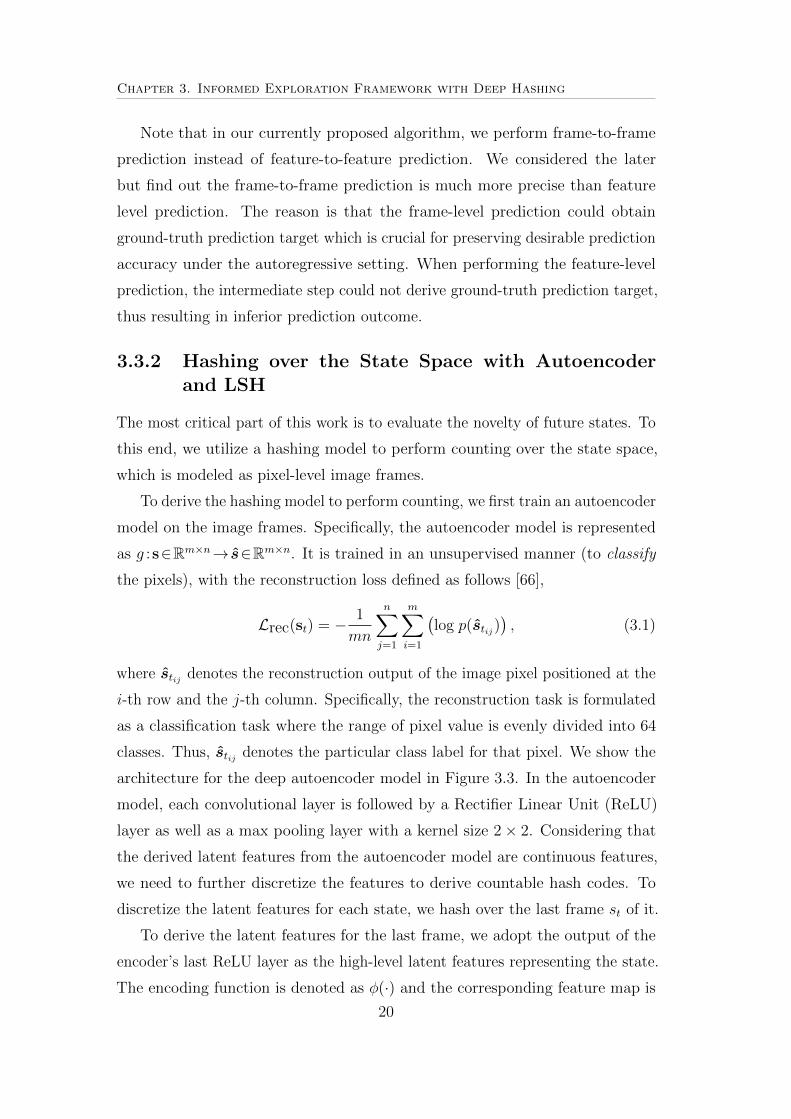
3.1 The multi-step prediction loss measured in MSE for the action-
conditional prediction model. . . . . . . . . . . . . . . . . . . . 26
3.2 Performance score for the proposed approach and baseline RL
approaches. . . . . . . . . . . . . . . . . . . . . . . . . . . . . . 30
4.1 Performance scores for di↵erent deep RL approaches on 6 hard
exploration domains from Atari 2600.. . . . . . . . . . . . . . . 42
5.1 Performance scores for the three task settings in ViZDoom eval-
uated over 6 independent runs. Overall, only our approach and
’RND’ could converge to 100% under all the settings. . . . . . . 54
5.2 The approximated environment steps taken by each algorithm to
reach its convergence standard under each task setting. Notably,
our proposed algorithm could achieve an average speed up of 2.89x
compared to ‘ICM’, and 1.90x compared to ‘RND’. . . . . . . . 54
6.1 Performance scores for policy networks with di↵erent architectures
in each game domain. . . . . . . . . . . . . . . . . . . . . . . . . 74
7.1 Zero-shot policy transfer score evaluated at the target domain for
DeepMind Lab task. . . . . . . . . . . . . . . . . . . . . . . . . 90
7.2 Zero-shot policy transfer score evaluated at the target domain for
ViZDoom. . . . . . . . . . . . . . . . . . . . . . . . . . . . . . . . 91
1

Chapter 1
Introduction
1.1 Deep Reinforcement Learning
Reinforcement learning (RL) o↵ers a mathematical framework for an artificial
agent to automatically develop meaningful task-driven behaviors given limited
supervision of task-related reward signals [1]. An RL agent progressively interacts
with the initially unknown environment, and continuously adjusts its policy model
with the objective of maximizing the total cumulative rewards collected from
the environment. Over the past decades, RL has achieved persistent success
across a broad range of application domains, such as robotics control [2, 3, 4],
autonomous driving [5, 6], etc. Despite its success, conventional approaches are
mostly developed upon human designed features and could not scale to more
complex problems with high dimensional input. Such limitation is mainly due
to the reason that the traditional way of modeling policy lacks of complexity to
handle complex relationships.
Over the recent years, deep neural network has emerged as an e�cient function
approximator to advance the state-of-the-art performance in various task domains
such as object detection [7, 8, 9], speech recognition [10, 11] and language
translation [12, 13]. Utilizing deep neural networks as the function approximator
to represent RL policy lead to the emergence of today’s deep RL research.
Powered up by the superior representation ability of deep neural networks,
deep RL is capable to solve much more challenging tasks than conventional
RL approaches. The revolution of deep RL first started from the development
of DQN [14], where one single algorithm could be used to play a range of
Atari 2600 video games by only taking pixel-level frames as the input for the
2

Chapter 1. Introduction
model. Afterwards, successful applications of deep RL have emerged across
many application domains other than video games playing, such as recommender
systems [15, 16, 17], classification [18, 19, 20] and dialogue generation [21, 22].
One of the key reasons that lead to the success of deep RL is that it reveals
the e↵ort of handcrafting model features and enables the policy to be trained
in an end-to-end manner. However, this in turn leads to considerable di�culty
to the training of deep RL models. The state space, when modeled as low-level
sensory inputs such as image pixels and word tokens, could result in tremendous
size. Moreover, the complex nature of the problems, such as the long decision
horizon and sparse reward condition, further enlarges the search space for the
algorithm to experience through. Therefore, developing exploration strategy
that could e�ciently search through the tremendous solution space is crucial for
advancing today’s deep RL research. Also, considering that the training of deep
RL model would consume considerable computation resource and time, it is also
desirable to develop the generalization ability of the policy, so that knowledge
among di↵erent task domains could be exploited to derive better policy at a
lower cost. This motivates the research presented in this thesis. On the one
hand, the presented study aims to improve the exploration strategy of deep RL
algorithms via adopting advanced novelty model, distributed training techniques
or planning. On the other hand, we aim to improve the generalization ability of
the policy model by utilizing e�cient transfer learning techniques.
1.2 Exploration vs. Exploitation
RL involves an agent progressively interacting with an initially unknown envi-
ronment, in order to learn an optimal policy that can maximize the cumulative
rewards collected from the environment. Throughout the training process, the
RL agent alternates between two primal behaviors: exploration - to try out novel
states that could potentially lead to high future rewards; and exploitation - to
perform greedily according to the learned knowledge. The RL agent faces the
trade-o↵ between exploration and exploitation throughout the learning process.
It is impossible for the agent to learn an optimal policy without su�ciently
exploring through the state space. How to model the exploration behavior is a
critical issue for deriving deep RL policy model to solve complex problems.
3
Chapter 1. Introduction
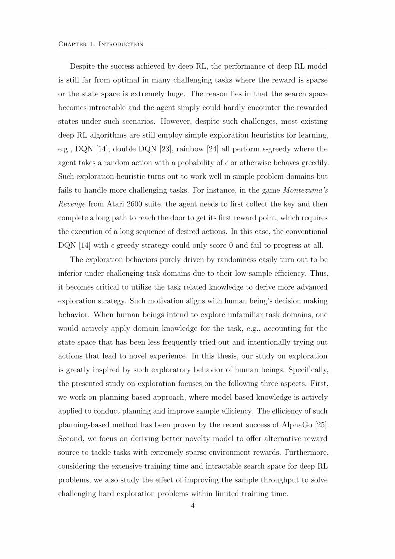
Despite the success achieved by deep RL, the performance of deep RL model
is still far from optimal in many challenging tasks where the reward is sparse
or the state space is extremely huge. The reason lies in that the search space
becomes intractable and the agent simply could hardly encounter the rewarded
states under such scenarios. However, despite such challenges, most existing
deep RL algorithms are still employ simple exploration heuristics for learning,
e.g., DQN [14], double DQN [23], rainbow [24] all perform ✏-greedy where the
agent takes a random action with a probability of ✏ or otherwise behaves greedily.
Such exploration heuristic turns out to work well in simple problem domains but
fails to handle more challenging tasks. For instance, in the game Montezuma’s
Revenge from Atari 2600 suite, the agent needs to first collect the key and then
complete a long path to reach the door to get its first reward point, which requires
the execution of a long sequence of desired actions. In this case, the conventional
DQN [14] with ✏-greedy strategy could only score 0 and fail to progress at all.
The exploration behaviors purely driven by randomness easily turn out to be
inferior under challenging task domains due to their low sample e�ciency. Thus,
it becomes critical to utilize the task related knowledge to derive more advanced
exploration strategy. Such motivation aligns with human being’s decision making
behavior. When human beings intend to explore unfamiliar task domains, one
would actively apply domain knowledge for the task, e.g., accounting for the
state space that has been less frequently tried out and intentionally trying out
actions that lead to novel experience. In this thesis, our study on exploration
is greatly inspired by such exploratory behavior of human beings. Specifically,
the presented study on exploration focuses on the following three aspects. First,
we work on planning-based approach, where model-based knowledge is actively
applied to conduct planning and improve sample e�ciency. The e�ciency of such
planning-based method has been proven by the recent success of AlphaGo [25].
Second, we focus on deriving better novelty model to o↵er alternative reward
source to tackle tasks with extremely sparse environment rewards. Furthermore,
considering the extensive training time and intractable search space for deep RL
problems, we also study the e↵ect of improving the sample throughput to solve
challenging hard exploration problems within limited training time.
4

Chapter 1. Introduction
1.3 Policy Generalization
Though generalization has long been considered as an important and desirable
property for RL policy, unfortunately, the application of today’s deep RL policy
model is highly restricted over its own training domain and the derived policy
conveys very limited capability of generalization. Developing the generalization
capability of deep RL policy not only helps to save the training e↵ort by being able
to reuse the models, but also brings noticeable improvement on task performance
by utilizing the transfer learning formalism, i.e., exploiting the commonalities
between related tasks so that knowledge learned from some source task domain(s)
could e�ciently help the learning in the target task domain. In this thesis, we
present a study on policy generalization problems for deep RL that covers the
following two types of policy generalization problems: policy distillation and
zero-shot policy transfer.
Policy distillation refers to the process for transferring knowledge from multi-
ple RL policies into a single multi-task policy via distillation technique. When
policy distillation is adopted under a deep RL setting, due to the giant parameter
size and the huge state space for each task domain, the training of the multi-task
policy network would consume extensive computational e↵orts. In this study, we
present a new solution with the attempt of improving the convergence speed and
representation quality of the multi-task policy model. To this end, we introduce
a novel multi-task policy architecture to improve the feature representation of the
policy model. Furthermore, we introduce a novel hierarchical sampling approach
to conduct experience replay, so that the sample e�ciency could be improved for
policy distillation with the advanced sampling approach.
Also, the presented study on policy generalization tackles the zero-shot
policy transfer problems, which refers to the type of challenging policy transfer
tasks where data from the target domain is strictly inaccessible for the learning
algorithm. In such problems, the RL policy is evaluated on a disjointed set of
target domain from the source domains, with no further fine-tuning performed
on the target domain data. For zero-shot policy generalization, even though the
source domains could convey significant commonalities with the target domain,
since there is completely no access to the target domain data, it becomes extremely
challenging to develop the generalization ability of the policy, especially for deep
5

Chapter 1. Introduction
RL problems where the input state is modeled as low-level representations. To
solve such problems, we introduce a novel adversarial training mechanism which
could derive domain invariant features and disentangle the task relevant and
irrelevant features with great e�ciency.
1.4 Contributions and Thesis Overview
In this thesis, I will present several algorithms that aim to improve deep RL algo-
rithm from the perspectives of exploration and policy generalization. Specifically,
for exploration, our study covers three algorithms that work on model-based
planning, distributed policy learning and sequence-level intrinsic novelty model,
respectively. For policy generalization, I will introduce two algorithms that
aim to tackle the policy distillation problem and zero-shot policy generalization
problem, respectively. All of the algorithms are designated for solving challenging
vision-based game playing tasks with high dimensional input space. The above
mentioned algorithms are presented from Chapters 3 to 7 in this thesis. Overall,
this thesis is organized as follows:
Chapter 2 presents a literature review on exploration approaches and policy
generalization approaches.
Chapter 3 presents a planning-based exploration algorithm which adopts deep
hashing techniques to perform count-based exploration in order to improve the
sample e�ciency.
Chapter 4 presents a distributed deep RL framework with an exploration
incentivizing mechanism. We adopt a novelty model formulated as random distil-
lation network and a policy model formulated as NoisyNet [26]. By embedding
them into the distributed framework, we aim to derive an algorithm with both
superior sample throughput and superior sample e�ciency, so that the policy
training could be updated from a large throughput of novel experiences.
6

Chapter 1. Introduction
Chapter 5 presents a sequence-level novelty model designated for solving par-
tially observable tasks with extremely sparse rewards. A dual-LSTM architecture
is presented, which consists of an open-loop action prediction module to flexibly
adjust the degree of prediction di�culty for the forward dynamics model.
Chapter 6 presents a novel algorithm for multi-task policy distillation. A new
multi-task network architecture as well as a hierarchical sampling approach is
introduced to improve the sample e�ciency of policy distillation.
Chapter 7 presents a zero-shot policy transfer algorithm. An adversarial
training mechanism is presented to derive domain invariant features via semi-
supervised learning. Then the policy is trained by taking the domain invariant
features as input under a multi-stage RL set up.
7
Chapter 2
Related Work
The study presented in this thesis is mainly related to exploration and transfer
learning problems for deep RL. In this chapter, I therefore review previous works
of exploration approaches and transfer learning approaches in Section 2.1 and
Section 2.2, respectively.
2.1 A Review of Exploration Approaches
The learning process for the RL agent is driven by performing two primary
types of behaviors: exploration, under which the agent attempts to seek novel
experience, and exploitation, under which the agent behaves greedily. How to
model the exploration behavior for deep RL agent is a crucial issue for deriving a
desirable policy with limited consumption of time and computational resources.
To model the exploration behavior, the simplest and most commonly adopted
way is to perturb the greedy action selection policy by adding random dithering
to it. A typical example under the discrete action setting is ✏-greedy exploration
strategy [1], where the agent takes a random exploratory action with probability
less than a specified value of ✏, or otherwise acts greedily according to the learned
knowledge, i.e.,
at =
(argmax
a[Q(s, a)] p � ",
random(a) p < ",
where p is a random value sampled from a distribution, e.g., uniform distribution,
and Q(s, a) denotes the value for action a at state s:
Q(s, a) = E⇡⇥ TX
t=0
�tR(st, at)|s0 = s, a0 = a⇤. (2.1)
8

Chapter 2. Related Work
For continuous control setting, a common way of such dithering is to add Gaussian
noise to the derived greedy action values. Besides the above-mentioned way of
performing exploration and exploitation alternatively, another prominent line
of introducing randomness for exploration is to adopt sampling on the learned
action distribution. A common way of performing such sampling under discrete
actions setting is to formulate the action distribution as a Boltzmann distribution,
where the probability for each action is defined as:
⇡(a|s) = eQ(s,a)/⌧
Pa e
Q(s,a)/⌧, (2.2)
where ⌧ is a positive temperature hyperparameter and Q(s, a) is the estimated
action value.
Such simple exploration strategies are easy to be developed, and they do not
rely greatly on the specific knowledge of the task domain. Therefore, they are
commonly adopted by many deep RL methods, e.g., DQN [14], A3C [27], Dueling-
DQN [28] and Categorical-DQN [29] all adopt the simple ✏-greedy exploration
strategy. However, such simple randomization nature can easily be insu�cient for
complicated deep RL problems, since the complex problems often engage a search
space with tremendous size. The ine�ciency of such approaches mainly come
from the low sample e�ciency for the simple perturbation or sampling, e.g., the
way of introducing exploratory randomization could neither depress those actions
that could easily be learned to be inferior, nor intuitively distinguish the state
space which have been su�ciently experienced from the rarely experienced places.
Therefore, a more sophisticated exploration strategy is desired to facilitate the
policy learning of deep RL algorithms in complex problem domains.
2.1.1 Exploration with Reward Shaping
Reward shaping is a prevailing type of method to solve the exploration challenge
in deep RL domains. Initially, the term shaping is proposed by experimental
psychologists, which is referred to as the process of training animals to do complex
motor tasks [30]. Later, when first introduced in the RL context [31, 32], shaping
refers to the approach of training the robot on a succession of tasks, where each
task is solved by the composed skill modeled as a combination of a subset of the
already learned elemental tasks together with the new elemental task. Nowadays,
9
Chapter 2. Related Work
the semantics of shaping, or reward shaping, has been extended beyond training
a succession of tasks. Reward shaping in RL is more commonly referred to as
supplying additional rewards to a learning agent to guide the policy learning
beyond the external rewards supplied by the task environment [33, 34].
Reward shaping is closely related to the intrinsically motivated [35] or
curiosity-driven RL. The intrinsic or curiosity model could be conveniently
modeled via reward shaping. Formally, to adopt reward shaping in deep RL, an
additional reward function is modeled to assign additional reward to each state
or state action pair, i.e.,: R+ : S ⇥ A ! R or R+ : S ! R. Thus in addition
to the external environment reward R(s, a), each state or state action pair is
associated with an additional reward bonus term R+(s, a) (or R+(s)). And the
overall optimization objective for RL after incorporating the additional reward
bonus becomes:
⌘(⇡) = Es0,a0,...
h 1X
t=1
R(st, at) +R+(st, at)i, (2.3)
where ⇡ is the policy to be optimized and the expectation is taken over the
trajectories sampled from policy ⇡.
Developing agent’s intrinsically motivated or curiosity-driven behavior with
reward shaping turns out to be extremely beneficial for solving complex deep RL
problems. The intrinsic novelty model could encourage the agent to continuously
search through the state space and acquire meaningful reward gaining experience.
This works extremely well for solving the challenging problems with sparse
reward, since the agent could consistently receive the intrinsic reward while the
external environment hardly gives any feedback for policy learning at the initial
stage.
In recent years, a great number of exploration approaches with reward shaping
have emerged, which have significantly improved the state-of-the-art performance
of deep RL algorithms in many challenging task domains. In [36], a count-based
approach is proposed by hashing with deep autoencoder model. In [37], a neural
density model is proposed to approximately compute a pseudo-count to represent
the novelty of each state. [38] derive the novelty of state from prediction error
of environment dynamics model or self-prediction models. In this study, we also
10

Chapter 2. Related Work
present a novel reward shaping model based on prediction-error of environment
dynamics.
Our work is mostly related to [38] and all the works are evaluated in partially
observable domains. However, the model in [38] engages a feed forward model to
perform 1-step forward prediction. Thus, it conveys relatively limited capability
to model the state transition in partially observable domains. Our proposed
model engages a sequence-level novelty prediction model. Moreover, we engage
an open-loop action prediction module , which could flexibly control the di�culty
of novelty prediction to cater for di↵erent problems. Our approach has been
demonstrated to work well not only in partially observable domains but also for
tasks with nearly full observation like Atari 2600 games.
2.1.2 Model-based Exploration
Model-based exploration approaches utilize the knowledge about the learning
process (i.e., MDP) to construct an exploration strategy. A prominent type of
such approach is the planning-based approaches. In [39], Guo et al. integrate
an o↵-line Monte Carlo tree search planning method based on upper confidence
bounds for tree (UCT) [40] with DQN to play Atari 2600 games. UTC-agent
by itself is not capable to be used for real-time game play. The o✏ine playing
data generated by the UTC agent is utilized to train a deep classifier that is
capable for real-time play. The Monte Carlo planning could generate reliable
estimate for the utility of taking each action by e�ciently summarizing future
roll-out information. In [41], Oh et al. train a deep predictive model for
conducting informed exploration, which is built upon the standard ✏-greedy
strategy. Once ✏-greedy decides to take an exploratory action, the predictive
model generates future roll-outs for each action direction and the Gaussian
kernel distance between the future roll-out frames and a window of recently
experienced frames is used to derive a novelty metric for each action direction.
Thus the model-based planning enables the agent to pick up the most novel
action to explore in an informed manner. In [42], an Imagination-based Planner
(IBP) is proposed where agent’s external policy making model and an internal
environment prediction model is jointly optimized. Specifically, the policy making
model could determine at each step whether to take a real action or take an
11

Chapter 2. Related Work
imagination step to perform a variable number of prediction over the environment
roll-outs. The imagination context could be aggregated to form a plan context
which could facilitate the agent’s decision on the real action. In [43], Weber et al.
proposed Imagination-Augmented Agents (I2As), which aims to utilize the plan
context derived from model-based knowledge to facilitate decision making. I2As
composes the predicted roll-out information into an encoding feature, which is
used as part of the input for the deep policy network.
One of the key advantages of the planning-based approach is that the model-
based knowledge could help to establish a relationship between policy and future
rewards, and thereby e�ciently encourage the novel experience seeking behavior.
In this thesis, we also introduce a model-based planning approach to carry out
exploration. Our work is mostly related to [41]. While [41] utilizes a Gaussian
kernel distance metric to evaluate the novelty of future states, our proposed
method utilizes deep hashing techniques to hash over the future frames and
infer the novelty of future states in a count-based manner. The count-based
evaluation of novelty demonstrates to be a more reliable metrics to represent
novelty. Compared to the count-based approaches [36, 44], our approach utilize
hashing for conducting planning instead of conducting reward shaping.
2.1.3 Distributed Deep RL
Nowadays, one of the key challenges for the training of deep RL algorithm is the
limitation in terms of the sample throughput. Even with advanced exploration
mechanism, the training of conventional deep RL algorithms still su↵ers from
extremely slow convergence, i.e., training a model easily takes several days
or weeks. The advancement of distributed deep RL algorithms has brought
significant benefit in increasing the sample throughput. Furthermore, with such
techniques, the agent also significantly benefits from the increased search space
and in tern derives policy with better performance.
In [45], IMPALA is proposed, which formulates the actor-critic learning in
a distributed manner. Furthermore, an importance weighted sample update is
incorporated to further improve the sample e�ciency. In [46], Ape-X framework
is proposed, which conducts importance weighted Q-learning update in a dis-
tributed manner. In [47], an RNN-based distributed framework is proposed to
12

Chapter 2. Related Work
conduct importance weighted Q-learning. The above mentioned distributed ap-
proaches lead to significant reduce of model training time as well as considerable
performance improvement in various challenging task domains. However, the
algorithms only incorporate simple exploration strategy, e.g., each actor agent
in Ape-X simply adopts ✏-greedy exploration, and the actor in IMPALA simply
performs Boltzmann sampling.
In this thesis, we present a distributed framework which aims to improve the
exploration behavior of the distributed deep RL algorithms. Specifically, our work
is built upon Ape-X with the aim of bootstrapping the performance of Ape-X in
extremely challenging exploration domains. To this end, we take the following
two e↵orts to improve the exploration of the algorithm. On the one hand, we
adopt random distillation network to construct a novelty model, which is good at
identifying novel states while o↵ering a relatively computational lightweight way
for online inference/optimization. On the other hand, we parameterize the policy
model as NoisyNet [26], which turns out to work extremely well in generating
rewarded experience even in those sparse reward hard exploration task domains.
2.2 A Review of Policy Generalization
2.2.1 Policy Distillation
The idea of policy distillation comes from model compression in ensemble learn-
ing [48]. Originally, the application of ensemble learning to deep learning aims to
compress the capacity of a deep neural network model through e�cient knowledge
transfer [49, 50, 51, 52]. In recent years, policy distillation has been successfully
applied to solve deep RL problems [53, 54]. The goal is often defined as training
a single policy network that can be used for multiple tasks at the same time.
Generally, such policy transfer engages a transfer learning process that has a
student-teacher architecture. Specifically, the policy is first trained from each
single problem domain as teacher policies, and then the single-task policies are
transferred to a multi-task policy model known as student policy. In [54], a
transfer learning is proposed which uses a supervised regression loss. Specifically,
the student model is trained to generate the same output as the teacher model.
In the existing policy distillation approaches, the multi-task model almost
shares the entire model parameters among the task domains. In this way, the
13

Chapter 2. Related Work
entire policy parameters need to be updated during the multi-task learning,
which could lead to considerable training time. Moreover, such setting assumes
multiple tasks to share the same statistical base by sharing all the convolutional
filters among tasks. However, the pixel-level inputs for di↵erent tasks actually
di↵er a lot. Thus, sharing the entire network parameter might fail to model
some important task-specific features and lead to inferior performance. In this
thesis, we present an algorithm to improve upon the existing policy distillation
method. Specifically, we propose a novel model architecture, where we remain the
convolutional filters as task-specific and share the fully-connected layers as multi-
task policy network. This turns out to significantly reduce the model convergence
time. Furthermore, utilizing the task-specific features would result in better
model performance. To further improve the sample e�ciency of the multi-task
training, our work also introduces a new hierarchical sampling approach.
2.2.2 Zero-shot Policy Generalization
In this thesis, we present a new algorithm that tackles zero-shot policy generaliza-
tion problem. Zero-shot policy transfer is an important but relatively less studied
topic among RL literature. Developing domain generalization capability for the
policy under zero-shot deep RL setting is a non-trivial task. First, the low-level
state inputs, often modeled as image pixels, would saliently encode abundant
domain specific information irrelevant to policy learning, and thus makes the
policy hard to generalize. Second, since target domain data is strictly inaccessible
for zero-shot policy training, those commonly adopted domain adaptation tech-
niques, e.g., latent feature alignment [55, 56, 57] and minimizing discrepancies
between latent distributions of domains [58], could hardly help.
The existing zero-shot policy transfer methods with non-deep RL setting
mainly focus on learning task descriptors or explicitly establishing inter-task
relationship. In [59], skills are parameterized by task descriptors, and classifiers
or regression models are combined to learn the lower-dimensional manifold on
which the policies lie. In [60], dictionary learning with sparsity constraints is
adopted to develop inter-task relationship. However, with deep RL setting, such
attempts are often not applicable due to the di�culty of explicitly learning task
descriptors or relationship. The existing methods with deep RL setting often rely
14

Chapter 2. Related Work
on training the policy across multiple source domains to make it generalizable.
In [61], the explicitly specified goal for each task is used as part of input to the
policy, and a universal function approximator is learned to map the state-goal pair
to policy. In [62], a hierarchical controller is constructed with analogy-making
goal embedding techniques. Compared to the above mentioned attempts, our
work mainly di↵ers in two aspects. First, we tackle a line of problems with
di↵erent zero-shot setting [63], where task distinction is introduced by input
state distribution shift. The most related work to ours is [63], where a Beta-
VAE [64] is trained to generate disentangled latent features. In our work, we
move beyond unsupervised learning and propose a weakly supervised learning
mechanism. Second, our approach improves upon traditional attempts of deriving
generalizable policy via training it across multiple source domains. Instead, we
enable the transferable policy to be trained on only one source domain.
15

Chapter 3
Informed ExplorationFramework with Deep Hashing1
3.1 Motivation
To tackle challenging deep RL tasks, an e�cient exploration mechanism should
continuously encourage the agent to select exploration actions that lead to less
frequent experience which could possibly bring higher cumulative future rewards.
However, constructing such exploration strategy is extremely di�cult, since the
task of letting the intelligent agent to know about the future consequence and
evaluate the novelty of future states are both considered as non-trivial tasks. In
this chapter, we present a novel exploration algorithm that could intuitively
direct the agent to select exploration action which could lead to novel future
states. Generally, the RL agent no longer performs random action selection for
exploration. Instead, the presented algorithm could deterministic ally suggest an
action which could lead to the least frequent future states.
To this end, we develop the following two capabilities of an RL agent: (1) to
predict over the future transitions, (2) to evaluate the novelty for the predicted
future frames with a count-based manner. Then we incorporate the above two
modules into a unified exploration framework. The overall decision making
process for exploration is presented in Figure 3.1.
Evaluating the novelty of states in a count-based manner under deep RL
setting is a non-trivial task. Since the state is often modeled as low-level sensory
inputs, counting over the low-level sensory state is less e�cient. To derive an
1The content in this chapter has been published in [65].
16

Chapter 3. Informed Exploration Framework with Deep Hashing
Figure 3.1: An overview of the the decision making procedure for the proposedinformed exploration algorithm. For exploration, the agent needs to choose froma(1)t to a(|A|)
t state St, as the exploration action. In the figure, the states insidethe dashed rectangle indicates predicted future states, and the color of circles(after St) indicates the frequency/novelty of states, the darker the higher novelty.To determine the exploration action, the agent first predicts future roll-outs withthe action-conditional prediction module. Then, the novelty of the predictedstates is evaluated via deep hashing. In the given example, action a(2)t is selectedfor exploration, because its following roll-out is the most novel.
e�cient novelty metric over the low-level states, we present a deep hashing
technique based on a convolutional autoencoder model. Specifically, a deep
prediction model is first trained to predict the future frames given each state-
action pair. Then, hashing is performed over the predicted frames by utilizing the
deep autoencoder model and locality sensitive hashing [36]. However, performing
hashing over the predicted frames would face a severe challenge. When the
learned hash function is counting over the actually visited real states, the novelty
is queried over the predicted fake states. Hence, in this algorithm, we engage
an additional training phase to address the problem of the hash code mismatch
between the real and fake states. The count value derived from hashing is used
to derive a reliable metric to evaluate the novelty of each future state, so that
the exploration could inform the agent to explore the actions that lead to least
frequent future states. Compared to the conventional exploration approaches
with random sampling such as ✏-greedy, our presented approach could select the
exploration action in a deterministic manner, and thus results in higher sample
e�ciency.
17

Chapter 3. Informed Exploration Framework with Deep Hashing
3.2 Notations
We consider Markov Decision Process (MDP) with a discounted finite-horizon
and discrete actions. Formally, we define the MDP as the following tuple
(S,A,P ,R, �), where S represents a set of states which are modeled as high-
dimensional image pixels, A is a set of actions, P represents a state transition
probability distribution with each value P(s0|s, a) specifying the probability of
transiting to state s0 after taking action a at state s, R is a real-valued reward
function that maps each state-action pair to a reward in R, and � 2 [0, 1] is a
discount factor. The goal of the RL agent is to learn a policy ⇡ which maximizes
the expected total future rewards under the policy: E⇡[PT
t=0 �tR(st, at)], where
T specifies the time horizon. For di↵erent RL algorithms, policy ⇡ can be
defined in di↵erent manner. For instance, the policy for actor-critic method
is normally defined as sampling from a probability distribution characterized
by ⇡(a|s), whereas that for Q-learning is defined as ✏�greedy which combines
uniform sampling with greedy action selection.
Under deep RL setting, at each time step t, the state observation received by
the agent is represented as St 2 Rr⇥m⇥n, where r is the number of consequent
frames which we use to represent a Markov state, and each frame has dimension
of m⇥n. After receiving the state observation, the agent selects an action at 2 Aamong all the l actions to take. Then the environment would return a reward
rt 2 R to the agent.
3.3 Methodology
3.3.1 Action-Conditional Prediction Network for Predict-ing Future States
The proposed informed exploration framework incorporates an action-conditional
deep prediction model to predict the future frames. The architecture for the
prediction model is shown in Figure 3.2.
To be specific, the deep prediction model takes a state-action pair as input to
predict the next frame f : (St, at)! St+1, where the input state St is modeled
as a concatenation of r consequent image frames, and the action at is modeled
18

Chapter 3. Informed Exploration Framework with Deep Hashing
Figure 3.2: Deep neural network architectures for the action-conditional predic-tion model to predict over the future frames.
as a one-hot vector at 2 Rl, where l denotes the total number of actions in the
task domain. The output of the model is denoted as s 2 Rm⇥n.
The proposed prediction model works in a autoregressive manner. The new
state St+1 could simply be formed by concatenating the newest predicted frame
with its recent r�1 frames. The state features need to be interact with the
action features to form a joint feature representation. To this end, we adopt
an action-conditional feature transformation as proposed in [41]. Specifically,
we first process the state input through three stacked convolutional layers to
derive a feature vector hst 2 Rh. Then linear transformation is performed on the
state feature hst and the one-hot action feature at via multiplying the features
with their corresponding transformation matrix Wst 2 Rk⇥h and Wa
t 2 Rk⇥l.
After the linear transformation, the two types of features convey the same
dimensionality. Then the transformed state and action features are adopted to
perform a multiplicative interaction to derive a joint feature as follows,
ht = Wsth
st �Wa
that .
The joint feature ht synthesis information from state feature and action feature.
It is then passed through three stacked deconvolutional layers with each followed
by a sigmoid layer. The output to the model is a single frame with shape 84⇥ 84.
To perform multi-step future prediction, the prediction model composes the new
state input autoregressively using its prediction result as part of its input.
19
Chapter 3. Informed Exploration Framework with Deep Hashing
Note that in our currently proposed algorithm, we perform frame-to-frame
prediction instead of feature-to-feature prediction. We considered the later
but find out the frame-to-frame prediction is much more precise than feature
level prediction. The reason is that the frame-level prediction could obtain
ground-truth prediction target which is crucial for preserving desirable prediction
accuracy under the autoregressive setting. When performing the feature-level
prediction, the intermediate step could not derive ground-truth prediction target,
thus resulting in inferior prediction outcome.
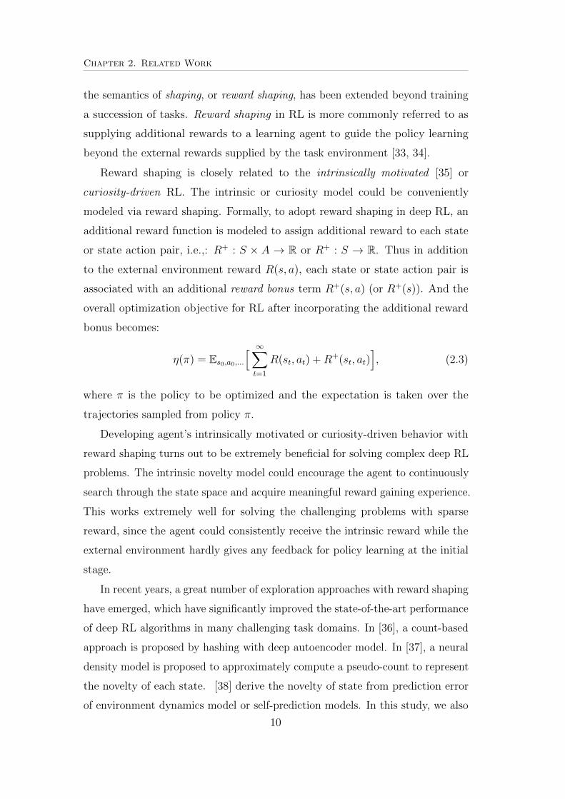
3.3.2 Hashing over the State Space with Autoencoderand LSH
The most critical part of this work is to evaluate the novelty of future states. To
this end, we utilize a hashing model to perform counting over the state space,
which is modeled as pixel-level image frames.
To derive the hashing model to perform counting, we first train an autoencoder
model on the image frames. Specifically, the autoencoder model is represented
as g :s2Rm⇥n! s2Rm⇥n. It is trained in an unsupervised manner (to classify
the pixels), with the reconstruction loss defined as follows [66],
Lrec(st) = �1
mn
nX
j=1
mX
i=1
�log p(st
ij
)�, (3.1)
where stij
denotes the reconstruction output of the image pixel positioned at the
i-th row and the j-th column. Specifically, the reconstruction task is formulated
as a classification task where the range of pixel value is evenly divided into 64
classes. Thus, stij
denotes the particular class label for that pixel. We show the
architecture for the deep autoencoder model in Figure 3.3. In the autoencoder
model, each convolutional layer is followed by a Rectifier Linear Unit (ReLU)
layer as well as a max pooling layer with a kernel size 2⇥ 2. Considering that
the derived latent features from the autoencoder model are continuous features,
we need to further discretize the features to derive countable hash codes. To
discretize the latent features for each state, we hash over the last frame st of it.
To derive the latent features for the last frame, we adopt the output of the
encoder’s last ReLU layer as the high-level latent features representing the state.
The encoding function is denoted as �(·) and the corresponding feature map is
20

Chapter 3. Informed Exploration Framework with Deep Hashing
Figure 3.3: Deep neural network architectures for the autoencoder model, whichis used to conduct hashing over the state space.
represented as vector zt2Rd, i.e., �(st) = zt. Then, to perform discretization
over zt, we adopt locality-sensitive hashing (LSH) [67] upon zt. Specifically, we
define a random projection matrix A 2 Rp⇥d i.i.d. entries drawn from a standard
Gaussian N (0, 1). Then the features z are projected through A, with the sign
of the outputs forming a binary code, c 2 Rp. Then counting is performed by
taking the discrete code c as hash code.
During the RL training, we create a hash table H to store the counts.
Specifically, the count for a state st is denoted as t. It can be queried and
updated online throughout the policy training phase. When a new observation
st arrives, the hash table H would increase the count t by 1 if ct exists in its
key set, or otherwise registering ct and set its count to be 1. Overall, the process
for counting over a state St is represented in the following manner:
zt = �(st), ct = sgn(Azt), and t = H(ct). (3.2)
3.3.3 Matching the Prediction with Reality
When we perform counting, we count over the actually seen frames, i.e., real
frames, to update the hash table. However, when we query the hash table to
derive the novelty, we query it over the predicted frames, which are fake. This
leads to a mismatch of the hash code between the counting and inference phase.
In order to derive meaningful novelty value, we need to match the predictions
with realities, i.e., to make the hash codes for the predicted frames to be the
same as their corresponding ground-truth seen frames.
21

Chapter 3. Informed Exploration Framework with Deep Hashing
To match the prediction with reality, we introduce an additional training
phase for the deep autoencoder model g(·). To this end, we force the encoding
function �(·) to generate close features between a pair of predicted frame and its
ground-truth seen frames. (Note that we could derive such pairs by collecting
data online during policy training). We introduce the following code matching
loss function, which works with a pair of ground-truth seen frame and predicted
frame (st, st) in the following manner,
Lmat(st, st) = k�(st)� �(st)k2 (3.3)
Finally, the composed loss function for training the autoencoder could be derive
by combing (3.1) and (3.3),
L(st, st; ✓) = Lrec(st) + Lrec(st) + �Lmat(st, st), (3.4)
where ✓ represents the parameters for the autoencoder.
Such code matching phase is crucial for deriving desirable novelty metrics.
Note that even though the prediction model could be well trained and generate
nearly perfect frames, hashing with the autoencoder with LSH would still lead to
distinct hash codes (we have evaluated this in all the task domains and details
are presented in Section 3.4.3). Therefore, the e↵ort for matching prediction
with reality is necessary. Moreover, it is a non-trivial task to match the state
code while ensuring a satisfying reconstruction behavior. If we simply fine-tune
a fully trained autoencoder with the reconstruction loss Lrec by optimizing
according to the additional code matching loss Lmat, it would instantly disrupt
the reconstruction behavior of the autoencoder even before the code loss could
decrease to the expected standard. Also, training the autoencoder from scratch
with both losses Lrec and Lmat turn out to be di�cult as well, since the loss
Lmat is initially very low while Lrec is initially very high. This makes the
network hardly find a meaningful direction to consistently decrease both losses
with a balance. Therefore, considering the above challenges, in this work, we
propose to train the autoencoder with two phases. The first phase optimizes
according to Lrec with input from seen frames until convergence. And the second
phase adopts the composed loss function L as proposed in (3.4) to match the
predicted hash code from its ground-truth.
22

Chapter 3. Informed Exploration Framework with Deep Hashing
3.3.4 Computing Novelty for States
Once the action-conditional prediction model f(·) and the deep autoencoder
model g(·) are pre-trained, the agent could utilize the two models to perform
informed exploration.
The exploration algorithm controls exploration vs. exploitation balance with
a decaying hyperparameter ✏. At each step, the agent would explore with a
probability of ✏, or otherwise performs greedy according to its learned policy.
When selecting exploration action, the agent would strategically choose the
one with the highest novelty to explore. Such selection is deterministic. To
select exploration action in the informed manner, given state St, the agent first
performs multi-step roll-out with length H to predict the future trajectories with
the action-conditional prediction model. The roll-out is performed over all the
possible actions aj 2 A. Then, with the predicted roll-outs, we could derive the
novelty score for an action aj given state St. Formally, the novelty is denoted by
⇢(aj|St),
⇢(aj|St) =HX
i=1
�i�1
q (j)t+i + 0.01
, (3.5)
where (j)t+i is the count derived for the i-th future state S(j)
t+i along the predicted
trajectory for the j-th action following (3.2), H denotes a predefined roll-out
length, and � denotes a real-valued discount rate. With the proposed novelty
function, the novelty score for a state would be inversely correlated to its count
and the novelty for a trajectory is represented as a sum over that for each state
evaluated in a discounted manner. After evaluating the novelty for all the actions,
the agent could deterministically select the one with the highest novelty score
to take. The overall action selection policy for the RL agent with the proposed
informed exploration strategy is defined as follows:
at =
8<
:
argmaxa
[Q(St, a)] p � ",
argmaxa
[⇢(a|St)] p < ",
where p is a random value drawn from uniform distribution Uniform (0,1), and
Q(St, a) is the output of the action-value.
23

Chapter 3. Informed Exploration Framework with Deep Hashing
3.4 Experimental Evaluation
3.4.1 Task Domains
The proposed exploration algorithm is evaluated on the following 5 representative
games from Atari 2600 series [68] in which the policy training would not converge
to desirable performance standard with the conventional ✏-greedy exploration
strategy:
• Breakout : a ball-and-paddle game where a ball bounces in the space and
the player moves the paddle in its horizontal position to avoid the ball
from dropping out of the paddle. The agent loses one life if the paddle fails
to collect the ball. The agent is rewarded when the ball hits bricks. The
action space consists of 4 actions: {no-op, fire, left, right}.
• Freeway : a chicken-crossing-high-way game where the player controls a
chicken to cross a ten lane high-way. The high-way is filled with moving
tra�c. The agent is rewarded if it could reaches the other side of the
high-way. It would lose life if hit by tra�c. The action space consists of
three actions: {no-op, up, down}.
• Frostbite: the game consists of four rows of ice blocks floating horizontal
on the water. The task of player is to control the agent to jump on the ice
blocks via avoiding deadly clams, snow geese, Alaskan king crabs, polar
bears, and the rapidly dropping temperature. The action space consists of
the full set of 18 Atari 2600 actions.
• Ms-Pacman: the player controls an agent to traverse through an enclosed
2D maze. The objective of the game is to eat all of the pellets placed in the
maze while avoiding four colored ghosts. The pellets are placed at static
locations whereas the ghosts could move. There is a specific type of pellets
that is large and flashing. If eaten by player, the ghosts would turn blue
and flee and the player could consume the ghosts for a short period to earn
bonus points. The action space consists of 9 actions: {no-op, up, right, left,down, upright, upleft, downright, downleft}.
24

Chapter 3. Informed Exploration Framework with Deep Hashing
• Q-bert :the game is to use isometric graphics puzzle elements formed in a
shape of pyramid. The objective of the game is to control a Q-bert agent to
change the color of every cube in the pyramid to create a pseudo-3D e↵ect.
To this end, the agent hops on top of the cube while avoiding obstacles and
enemies. The action space consists of six actions: {no-op, fire, up, right,left, down}.
Based on the taxonomy of exploration as proposed in [44], four of the five
games, Freeway, Frostbite, Ms-Pacman and Q-bert, are classified as hard explo-
ration games. The game Freeway has sparse reward and all the others have dense
reward. Though Breakout has not been classified as a hard exploration game,
the policy training of it demonstrates significant exploration bottleneck, since it
engages a state space that is changing rapidly as the learning progresses, and
the performance of standard exploration algorithm falls far behind advanced
exploration techniques in this domain.
For all the tasks, we model the state as a concatenation of 4 consequent image
frames of size 84⇥ 84.
3.4.2 Evaluation on Prediction Model
To evaluate the performance of the action-conditional prediction model, we adopt
identical network architecture as the one shown in Figure 3.2.
When training the prediction model, we create a training dataset that contains
500,000 transition records collected from a fully trained agent with DQN algorithm
and standard ✏-greedy exploration. During data collection, ✏ is set to be 0.3
(following the setting from [41]). For optimization, we adopt Adam [69] with a
learning rate of 10�3 and a mini-batch size of 100.
To demonstrate the prediction accuracy, we present the pixel-level prediction
loss measured in terms of mean square error (MSE) in Table 3.1. The multi-step
prediction result with a prediction horizon of {1, 3, 5, 10} are presented. From
the results, we could see the prediction losses are within a small scale for all
the task domains. Furthermore, we could notice that as the prediction horizon
increases, the prediction loss would also increase, which is as expected.
25
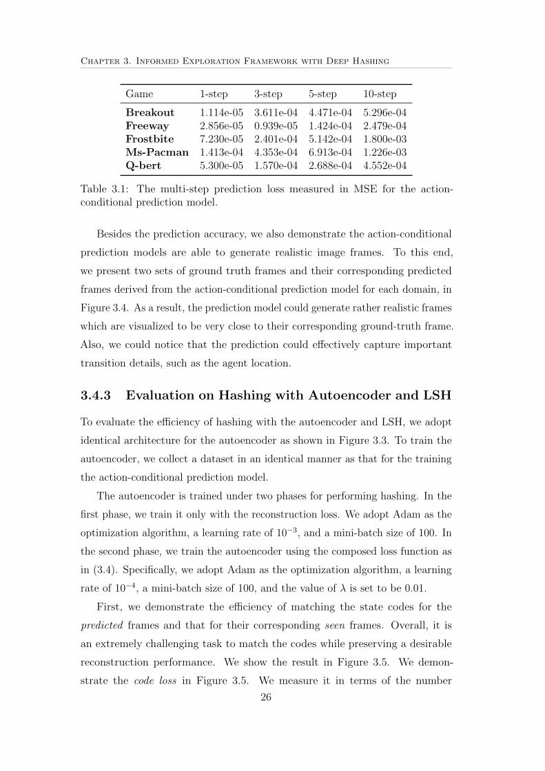
Chapter 3. Informed Exploration Framework with Deep Hashing
Game 1-step 3-step 5-step 10-step
Breakout 1.114e-05 3.611e-04 4.471e-04 5.296e-04Freeway 2.856e-05 0.939e-05 1.424e-04 2.479e-04Frostbite 7.230e-05 2.401e-04 5.142e-04 1.800e-03Ms-Pacman 1.413e-04 4.353e-04 6.913e-04 1.226e-03Q-bert 5.300e-05 1.570e-04 2.688e-04 4.552e-04
Table 3.1: The multi-step prediction loss measured in MSE for the action-conditional prediction model.
Besides the prediction accuracy, we also demonstrate the action-conditional
prediction models are able to generate realistic image frames. To this end,
we present two sets of ground truth frames and their corresponding predicted
frames derived from the action-conditional prediction model for each domain, in
Figure 3.4. As a result, the prediction model could generate rather realistic frames
which are visualized to be very close to their corresponding ground-truth frame.
Also, we could notice that the prediction could e↵ectively capture important
transition details, such as the agent location.
3.4.3 Evaluation on Hashing with Autoencoder and LSH
To evaluate the e�ciency of hashing with the autoencoder and LSH, we adopt
identical architecture for the autoencoder as shown in Figure 3.3. To train the
autoencoder, we collect a dataset in an identical manner as that for the training
the action-conditional prediction model.
The autoencoder is trained under two phases for performing hashing. In the
first phase, we train it only with the reconstruction loss. We adopt Adam as the
optimization algorithm, a learning rate of 10�3, and a mini-batch size of 100. In
the second phase, we train the autoencoder using the composed loss function as
in (3.4). Specifically, we adopt Adam as the optimization algorithm, a learning
rate of 10�4, a mini-batch size of 100, and the value of � is set to be 0.01.
First, we demonstrate the e�ciency of matching the state codes for the
predicted frames and that for their corresponding seen frames. Overall, it is
an extremely challenging task to match the codes while preserving a desirable
reconstruction performance. We show the result in Figure 3.5. We demon-
strate the code loss in Figure 3.5. We measure it in terms of the number
26

Chapter 3. Informed Exploration Framework with Deep Hashing
Figure 3.4: The prediction and reconstruction result for each task domain. Foreach task, we present 1 set of frames, where the four frames are organized asfollows: (1) the ground-truth frame seen by the agent; (2) the predicted frameby the prediction model; (3) the reconstruction of autoencoder trained onlywith reconstruction loss; (4) the reconstruction of autoencoder trained afterthe second phase (i.e., trained with both reconstruction loss and code matchingloss). Overall, the prediction model could perfectly produce frame output, whilethe fully trained autoencoder generates slightly blurred frames.
of mismatch in the hash codes between each pair of predicted frame and the
ground-truth frame. The presented values are derived by averaging over 10,000
pairs of binary codes. The result reveals an important fact that if we do not
perform the optimization of the second phase, it is impossible to perform hash-
ing with the deep autoencoder model, since the average code losses for all
the task domains are above 1, which indicates that the predicted frame would
derive distinct hash codes from its ground-truth frame, and thus makes the
novelty model meaningless, since the returned count does not represent the
true frequent. Also, the result in Figure 3.5 shows that after conducting the
second phase of training, the values of code loss could be significantly reduced.
For all the task domains, the values of the loss are reduced to be less than 1.
We also demonstrate the reconstruction errors in MSE after the training of
the autoencoder model with the two training phases. The result is presented
27

Chapter 3. Informed Exploration Framework with Deep Hashing
Figure 3.5: Comparison of the code loss for the training of the autoencodermodel (phase 1 and phase 2).
Figure 3.6: Comparison of the reconstruction loss (MSE) for the training of theautoencoder model (phase 1 and phase 2.
in Figure 3.6. We could observe that the reconstruction behavior for the au-
toencoder is slightly reduced by incorporating the second phase of training. To
demonstrate that even with the reduction of reconstruction performance, our
trained autoencoder model could still present reconstruction outcome which could
preserve significant features, we show the reconstruction outcome before and
after the second phase in Figure 3.4. Even the reconstructed frames are slightly
blurred after the second phase of training, they could still preserve essential game
features in the presented task domains.
Moreover, we demonstrate an illustrative example in Breakout to show that
the proposed hashing mechanism could derive meaningful hash codes for predicted
future frames (see Figure 3.7). Given a ground-truth frame, we predict the
future frames with length 5 by taking each action. It can be found that taking
di↵erent actions would lead to di↵erent trajectories of board positions. When
28

Chapter 3. Informed Exploration Framework with Deep Hashing
investigating the hash codes, we could observe three of the actions, no-op, fire
and left, lead to rather small visual change, and thereby, their corresponding
hash codes convey very little changes as well. The action right leads to the
most significant visual change, so the hash codes for its predicted trajectories
demonstrates much more change in color than the rest. Meanwhile, the frames
shown in Figure 3.7 also demonstrate that the action-conditional prediction
model could generate realistic multi-step prediction outputs, since the change of
board positions aligns with the actions being taken.
3.4.4 Evaluation on Informed Exploration Framework
To evaluate the e�ciency of the proposed exploration framework, we adopt into
the DQN algorithm [14] and compare the result by considering the following
baselines: (1) DQN which performs ✏-greedy with uniform action sampling,
Figure 3.7: The first block shows predicted trajectories in Breakout. In eachrow, the first frame is the ground-truth frame and the following five frames arethe predicted trajectories with length 5. In each row, the agent takes one ofthe following actions (continuously): (1) no-op; (2) fire; (3) right; (4) left. Theblocks below are the hash (hex) codes for the frames in the same row ordered ina top-down manner. The color map is normalized linearly by the hex value.
29

Chapter 3. Informed Exploration Framework with Deep Hashing
denoted by DQN-Random; (2) A3C [27], (3)A3C with density model derived
from hand-written Atari features [44], (4) pixelCNN-based exploration model [37],
(5) the mostly related informed exploration approach as proposed in [41], denoted
by DQN-Informed. Our proposed approach is denoted by DQN-Informed-Hash.
We adopt future prediction size of q = 3 when considering exploration. The
results are presented in Table 3.2.
From the results shown in Table 3.2, we could find that DQN-Informed-Hash
outperforms DQN-Informed with significant margin over all the testified domains.
Note that in the task Breakout, the agent with DQN-Informed fails to progress
in learning and always scores around 0. The reason may be that the kernel-
based pixel distance metric used by DQN-Informed would encourage the agent
to explore states that are dissimilar from their recent predecessors, but such
mechanism might be harmful for the agent to experience novel states. Also, our
proposed method DQN-Informed-Hash demonstrates the superior performance
with a deterministic exploration mechanism. This shows that counting over
the predicted future frames could help the agent to derive a meaningful novelty
evaluation mechanism.
Model Breakout Freeway Frostbite Ms-Pacman Q-bert
DQN-Random 401.2 30.9 328.3 2281 3876A3C 432.42 0 283.99 2327.8 19175.72
A3C-CTS 473.93 30.48 325.42 2401.04 19257.55pixelCNN 448.2 31.7 1480 2489.3 5876DQN-Informed 0.93 32.2 1287.01 2522 8238
DQN-Informed-Hash 451.93 33.92 1812.10 3526.60 8827.83
Table 3.2: Performance score for the proposed approach and baseline RL ap-proaches.
30

Chapter 4
Incentivizing Exploration forDistributed Deep ReinforcementLearning
4.1 Motivation
Recent advancement of distributed deep RL techniques exploits the computation
capability of the machines by running multiple environments in parallel and thus
enables the RL agent to process much more number of samples than conventional
RL algorithms. Besides the significantly reduced model training time, the parallel
computation of such distributed algorithms also brings noticeable benefit for
exploration and leads to performance increment across a broad range of task
domains.
Despite the various advantages, distributed deep RL algorithms still fail to
su�ce the exploration bottleneck on the extremely challenging tasks due to their
simple exploration strategy. That is, the existing approaches simply increase
the sample throughput while using standard exploration heuristics as backbone.
There lacks an e�cient novelty mechanism to encourage the distributed deep
RL agent to proactively search for novel experience and achieve near optimal
performance to tackle extremely challenging task domains.
Our study aims to improve the performance of the distributed deep RL
framework to derive better performance in a series of extremely challenging Atari
2600 game domains. In this chapter, we present a solution built upon Ape-X,
which performs prioritized experience replay under distributed Q-learning setting
and demonstrates great e�ciency in solving the series of Atari 2600 domains.
31

Chapter 4. Incentivizing Exploration for Distributed Deep ReinforcementLearning
Our objective is to improve the performance of Ape-X agent by designing a
more advanced exploration incentivizing mechanism. To this end, our e↵orts for
improving the exploration behavior of Ape-X fall to the following two aspects.
On the one hand, we incorporate a computationally friendly novelty model to
evaluate the novelty over the state space and perform reward shaping. On
the other hand, to deal with the cold start experienced by those tasks with
extremely sparse rewards (e.g., Montezuma’s Revenge), we conduct parameter
space exploration by using noise perturbed network weights to further incentivize
the model to explore.
4.2 Notations
We consider finite-horizon Markov Decision Process (MDP) with discrete actions
and discounted rewards. Formally, an MDP is defined by a tuple (S,A,P ,R, �),
where S is a set of states which are often modeled as high-dimensional image
pixels for deep RL algorithms, A is a set of actions, P is a state transition
probability distribution with each entry P(s0|s, a) specifying the probability for
transiting to state s0 given action a at state s, R is a real valued reward function
mapping each state-action pair to a reward in R, and � 2 [0, 1] is a discount
factor. The goal of the RL agent is to learn a policy ⇡, so that the expected
cumulative future rewards for each state-action pair by performing under ⇡:
E⇡[PT
t=0 �tR(st, at)]), could be maximized.
The cumulative future rewards for each state-action pair is also known as the
action value function or the Q-function, i.e., Q(s, a) = E⇥PT
t=0 �tR(st, at)|s0 =
s, a0 = a⇤. The value of each state V (s) is represented as the expectation of
action value over the policy ⇡, denoted as V (s) = Ea⇠⇡(s)[Q(s, a)]. The advantage
value for each state-action pair A(s, a) is defined by subtracting the state value
from the action value, i.e., A(s, a) = Q(s, a)�V (s). Given a state, the advantage
values for the actions sum to 0 and each value tells the relative importance for
the action at the given state.
32

Chapter 4. Incentivizing Exploration for Distributed Deep ReinforcementLearning
4.3 Distributed Q-learning with Prioritized Ex-perience Replay (Ape-X)
We first introduce Ape-X, which is the backbone algorithm for our proposed
solution.
Ape-X is a distributed Q-learning architecture that decouples acting from
learning: the actors run in parallel with each running on its own instances of
environment; the experience generated by the actors are stored in a centralized
replay memory; there is one learner that samples experience from the replay
memory and updates the Q-network. The actors take actions based on a shared
copy of network and the learner periodically synchronizes its weights to the
actors’ network.
Given an experience tuple et = {st, at, rt:t+n�1, st+n} where st is the state at
time t, at is the actor’s choice of action, rt:t+n�1 is the set of n-step environment
rewards, and st+n is the n-th future state transited from st and at, the centralized
learner conducts n-step Q-learning to minimize the following loss function:
L(✓i) =1
2
�Q⇤(st, at; ✓i�1)�Q(st, at; ✓i)
�2, (4.1)
where Q⇤(st, at; ✓i�1) is the n-step Q-value target computed by following Bellman
equation:
Q⇤(st, at; ✓i�1) = rt + �rt+1 + ...+ �n�1rt+n�1 + �n maxa0
Q(st+n, a0; ✓i�1). (4.2)
As such, the n-step Q-value target is represented by summing up the one-step
reward for the following n steps and then add the Q-value estimate for the
(t+ n)-th step evaluated from some target network parameterized by ✓i�1. In
the case where the episode ends with less than n steps, the multi-step rewards in
Equation 6.2 are truncated.
To further improve the data e�ciency, Ape-X adopts prioritized experience
replay [70] for the learner to sample data from the shared replay memory. With
prioritized experience replay, each experience is prioritized based on the scale of
the gradient for its TD-error (derived from the temporal di↵erence (TD) learning
loss function as defined in Equation 6.3):
w(et) =��5 L(✓i)
��, P (et) =(w(et) + ⌫)↵Pk (w(ek) + ⌫)↵
, (4.3)
33

Chapter 4. Incentivizing Exploration for Distributed Deep ReinforcementLearning
where w(et) is the sampling weight for et, ⌫ is a small constant to make each
weight strictly positive, ↵ is a small positive constant to stabilize the sampling
weight, and P (et) is the probability for the experience to be sampled. Thus, the
TD-error based prioritized experience replay enables the learner to sample the
most useful data to update the network.
Within its decoupled architecture, Ape-X adopts ✏-greedy to characterize the
exploration behavior for the distributed Q-learning agent. Specifically, each of the
parallel actors use a specific value of ✏ which is computed from some exponentially
scaled function. This setting mimics the situation where each actor explores a
specific region of the decision making space so that the search span could be
significantly expanded with the increased number of actor size. Furthermore, by
decoupling acting from learning, Ape-X enables both the throughput of actors to
generate new experience and the throughput for the learner to conduct Q-learning
to be increased simultaneously on a great scale. Thus, Ape-X results in much
shorter model training time. The exploration strategy of using di↵erent ✏ values
on di↵erent actor processes also leads to diverse experience to update the learner
network and results in promising performance scores consistently over the ALE
domain.
4.4 Distributed Q-learning with an ExplorationIncentivizing Mechanism (Ape-EX)
We introduce our solution, an improved framework over Ape-X with an advanced
exploration incentivizing mechanism, termed Ape-EX. Though the decoupled
architecture of Ape-X works well in most of the ALE domains, the exploration
behavior driven by the simple ✏-greedy exploration heuristic easily turns out to
be insu�cient to tackle the extremely challenging exploration tasks (e.g., Venture
and Gravitar, which are categorized as sparse-reward hard exploration domains
in [44] and the algorithm converges slowly to inferior performance). The reason
is that ✏-greedy leads to completely undirected exploration [71] with low sample
e�ciency.
Our solution to improve upon Ape-X is shown in Figure 4.1. Our framework
involves the same actor/learner/sampler processes as Ape-X. However, the di↵er-
ence is that our learner is defined with an exploration incentivizing mechanism.
34
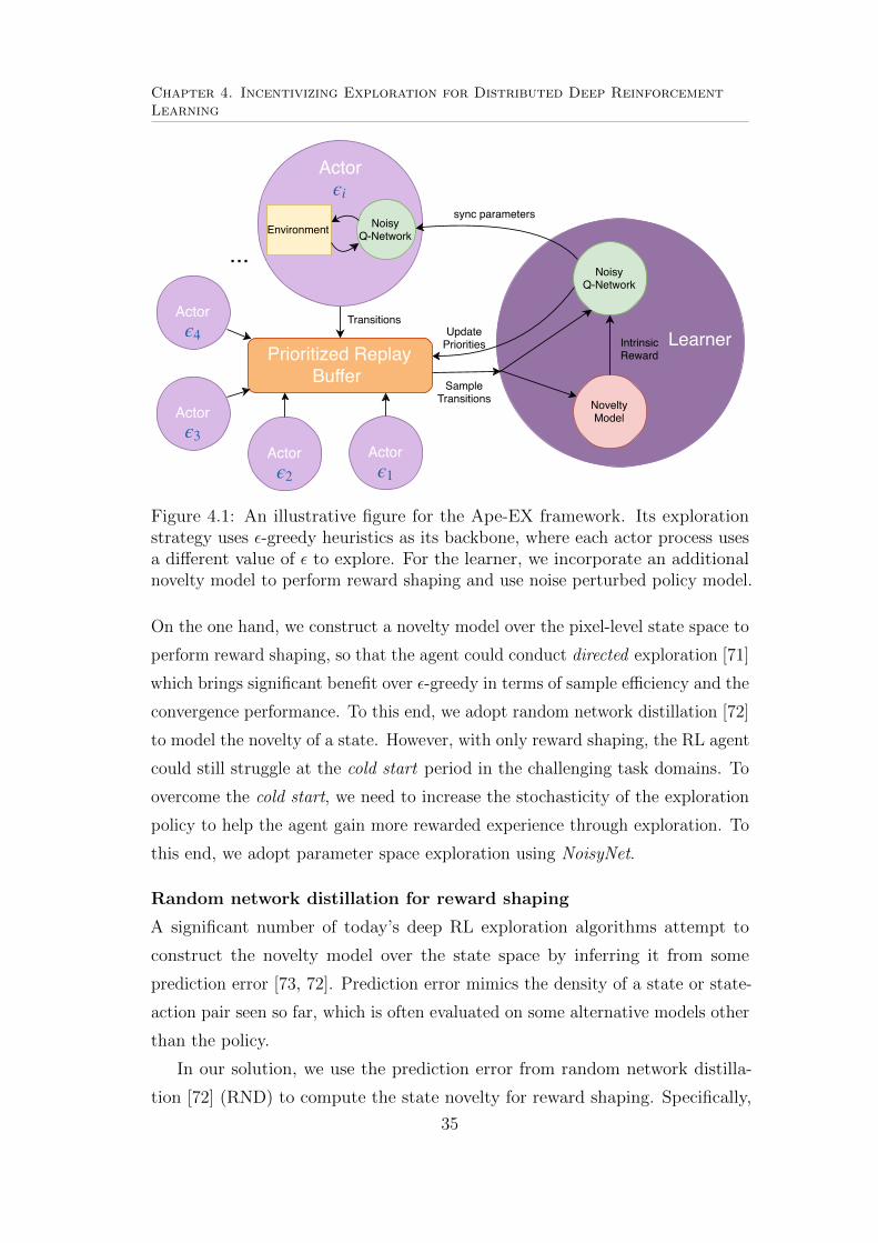
Chapter 4. Incentivizing Exploration for Distributed Deep ReinforcementLearning
Actor
Prioritized ReplayBuffer
Transitions
Learner
Noisy Q-Network
Novelty Model
Intrinsic Reward
Actor
Noisy Q-Network Environment
Actor
Actor
Actor Actor
sync parameters
Sample Transitions
Update Priorities
...
Text
Figure 4.1: An illustrative figure for the Ape-EX framework. Its explorationstrategy uses ✏-greedy heuristics as its backbone, where each actor process usesa di↵erent value of ✏ to explore. For the learner, we incorporate an additionalnovelty model to perform reward shaping and use noise perturbed policy model.
On the one hand, we construct a novelty model over the pixel-level state space to
perform reward shaping, so that the agent could conduct directed exploration [71]
which brings significant benefit over ✏-greedy in terms of sample e�ciency and the
convergence performance. To this end, we adopt random network distillation [72]
to model the novelty of a state. However, with only reward shaping, the RL agent
could still struggle at the cold start period in the challenging task domains. To
overcome the cold start, we need to increase the stochasticity of the exploration
policy to help the agent gain more rewarded experience through exploration. To
this end, we adopt parameter space exploration using NoisyNet.
Random network distillation for reward shaping
A significant number of today’s deep RL exploration algorithms attempt to
construct the novelty model over the state space by inferring it from some
prediction error [73, 72]. Prediction error mimics the density of a state or state-
action pair seen so far, which is often evaluated on some alternative models other
than the policy.
In our solution, we use the prediction error from random network distilla-
tion [72] (RND) to compute the state novelty for reward shaping. Specifically,
35

Chapter 4. Incentivizing Exploration for Distributed Deep ReinforcementLearning
given the state distribution D = {s0, s1, ...}, RND creates a random mapping
f⇠⇤ : st ! xt, where st is the low-level sensory input to represent the state and
xt 2 Rd is a set of low-dimensional features to represent st. The mapping is
characterized by parameters ⇠⇤, which is randomly initialized and kept fixed
during the policy learning. A popular choice of function f⇠⇤ is to use deep neural
networks. In our framework, the learner agent trains a prediction model f⇠(·) onthe sampled states to mimic the predefined function f⇠⇤ , so that the error from
f⇠(·) could be used to infer the novelty of a state.
Specifically, given a state st, the parameters for f⇠ is trained by minimizing
the following loss function:
⇠ = argmin⇠
Est
⇠Dkf⇠(st)� f⇠⇤(st)k2 + ⌦(⇠), (4.4)
where ⌦(·) is a regularization function. Based on the training loss, the novelty of
a state r+(st) is defined as:
r+(st) = �kf⇠(st)� f⇠⇤(st)k2, (4.5)
where � is a scaling factor. Hence, RND distills a random mapping function f⇠⇤
to another function f⇠. Since ⇠⇤ is kept fixed during training, the model involves
very light weighted trainable parameters for optimization, which makes it super
e�cient to be used by the learner in distributed framework.
Parameter space exploration
To further drive the exploration behavior of the distributed RL algorithm to
proactively seek more diverse experiences, we aim to increase the stochasticity
of the policy parameters. To this end, we adopt parameter space exploration
to the linear layers of the deep value network model to derive noise perturbed
parameter weights.
Conventionally, given input x, the output of a linear layer with parameters
(w, b) (i.e., the weights and bias) are computed as:
y = wx+ b. (4.6)
With the noise perturbed model, each linear layer parameter ✓ is defined as
✓ = µ + ⌃ � !, where ! is a zero-mean noise with fixed statistics. Thus each
36

Chapter 4. Incentivizing Exploration for Distributed Deep ReinforcementLearning
model parameter is characterized by a distribution ⇣def= (µ,⌃). As a result, the
network output for the noise perturbed linear layer is computed as:
y = (wµ + w� � !w)x+ (bµ + b� � !b). (4.7)
Furthermore, the noise for ✓i,j (connecting input i to output j) could be sampled
in the following factorized manner to reduce the sampling overhead:
!wi,j = f(!i)f(!j), !b
j = f(!j), (4.8)
where f could be some real-valued function, e.g., f(x) = sgn(x)p|x|. By
using the reparameterization trick, the noise perturbed formulation brings little
computational overhead for inference and optimization. Moreover, such sampling
approach leads to a more stochastic policy model which could help the RL agent
to explore more diverse experience. We demonstrate the stochasticity brought
by the noise perturbed formulation could bring significant benefit for the agent
to overcome the cold start period in those extremely sparse reward domains in
the experiment section.
The Ape-EX algorithm
Overall, the exploration incentivizing mechanism a↵ects the learner process by
updating the additional RND prediction model to compute reward bonus and
using a Q-network parameterized with noise perturbation. It a↵ects the actor
processes by using a sampling-based inference for their greedy action selection
and letting them adopt a policy which saliently encodes the novelty over the
state space.
By formulating the Q-value function following the dueling [28] architecture,
the learner process optimizes the following loss function:
L(✓i) =1
2krt + �rt+1 + ...+ �n�1rt+n�1 + r+(st+n)
+ �n maxa0
Q(st+n, a0; ✓i�1)�Q(st, at; ✓i)k2,
(4.9)
where the Q-function is formulated as:
Q(s, a) = V (s) + A(s, a)� Aµ(s, a), (4.10)
with Aµ(s, a) =P
a0 A(s, a0)/N being the mean of the advantage value outputs.
The complete Ape-EX algorithm is shown in Algorithm 1&2.
37

Chapter 4. Incentivizing Exploration for Distributed Deep ReinforcementLearning
Algorithm 1: Actor
1: procedure Actor(T, ✏)2: ✓ Learner.Parameters()3: st Environment.Reset()4: for t = 0 to T � 1 do5: ! ⇠ N(0, 1)6: at ✏-greedy(Q(st, · ; ✓,!))7: rt, st+1 Environment.Step(at)8: p ComputePriorities(st, rt, st+1)9: ReplayBu↵er.Add(st, at, rt, st+1, p)10: if Learner.ParametersHaveChanged() then11: ✓ Learner.Parameters()12: end if13: end for14: end procedure
Algorithm 2: Learner
1: procedure Learner(T, Ttarget)2: ✓, ⇠ InitializeNetworkParameters()3: ✓� ✓ . Initial target Q-network4: for t = 1 to T do5: idx, ⌧ ReplayBu↵er.Sample()6: rin RNDNovelty (⌧ ; ⇠)7: lRND ComputeRNDLoss(⌧ ; ⇠)8: ⇠ UpdateParameters(lRND, ⇠)9: !,!� ⇠ N(0, 1) . Sample noise for Q-network and target Q-network10: l ComputeLoss(⌧, rin; ✓,!, ✓�,!�)11: ✓ UpdateParameters(l, ✓)12: p ComputePriorities()13: ReplayBu↵er.UpdatePriorities(idx, ⌧, p)14: if t mod Ttarget == 0 then15: ✓� ✓16: end if17: end for18: end procedure
38

Chapter 4. Incentivizing Exploration for Distributed Deep ReinforcementLearning
4.5 Experimental Evaluation
4.5.1 Task Domains
For empirical evaluation, we evaluate our method on 6 of the most challenging
tasks from Atari 2600 games suite:
(i) Solaris: a space combat game with the galaxy being made up of 16
quadrants, each combining 48 sectors. The player uses a tactical map
to choose a sector to warp to, during which the fuel consumption must
be carefully managed. The player must descend to one of the 3 types
of planets: friendly federation planets, enemy Zylon planets and enemy
corridor planets. There are di↵erent enemies placed on the planets. The
ultimate goal of the game is to reach the planet Solaris and rescue its
colonists. The action space consists of the full set of 18 Atari 2600 actions.
(ii) Ms-pacman: the player controls an agent to traverse through an enclosed
2D maze. The objective of the game is to eat all of the pellets placed in the
maze while avoiding four colored ghosts. The pellets are placed at static
locations whereas the ghosts could move. There is a specific type of pellets
that is large and flashing. If eaten by player, the ghosts would turn blue
and flee and the player could consume the ghosts for a short period to earn
bonus points. The action space consists of 9 actions: {no-op, up, right, left,down, upright, upleft, downright, downleft}.
(iii) Montezuma’s Revenge: the player controls a character to move him from
one room to another where the rooms are located in an underground
pyramid of the 16th century Aztec temple of emperor Montezuma II. The
room is filled with enemies, obstacles, traps and dangers. The player could
score points by gathering jewels and keys or killing enemies along the way.
The action space consists of the full set of 18 Atari 2600 actions.
(iv) Gravitar : the player controls a small blue spacecraft to explore several
planets in a fictional solar system. When the player lands on a planet, he
will be taken to a side-view landscape. In side-view levels, the player needs
to destroy red bunkers, shoot, and pick up fuel tanks. Reward is gained
39

Chapter 4. Incentivizing Exploration for Distributed Deep ReinforcementLearning
when all bunkers are destroyed and the planet will blow up accordingly.
The player will move to other solar system if all the planets are destroyed.
The game terminates when fuel runs out or the spacecraft crashes into
terrain or shot by the enemy. The action space consists of the full set of 18
Atari 2600 actions.
(v) Private Eye: the player assumes the role of a private investigator who is
working on the task of capturing a criminal mastermind. The player needs
to search the city for specific clue of crimes and look for the object stolen.
Also, each stolen object needs to be returned to its rightful owner. After
locating all object and items, the player must capture the mastermind and
take him to jail. The action space consists of the full set of 18 Atari 2600
actions.
(vi) Frostbite: the game consists of four rows of ice blocks floating horizontal
on the water. The task of player is to control the agent to jump on the ice
blocks via avoiding deadly clams, snow geese, Alaskan king crabs, polar
bears, and the rapidly dropping temperature. The action space consists of
the full set of 18 Atari 2600 actions.
All of the games are categorized as hard exploration games from the taxonomy
proposed in [44]. Specifically, two of the games, Ms-pacman and Frostbite, have
dense reward, while all the others have sparse reward. Under the sparse reward
setting, it is extremely hard for the agent to e�ciently explore through the
decision space and progress in policy learning. And the game Montezuma’s
Revenge is known as an infamously challenging exploration task.
4.5.2 Model Specifications
Our Ape-EX model involves 384 actor processes and 1 learner process. Each actor
i 2 {1, ..., N} executes ✏i-greedy policy, where ✏i = ✏1+i�1N�1↵ with ✏ = 0.4, ↵ = 7.
The trainable models are the RND’s prediction network and the Q-network which
is modeled as NoisyNet. The learner synchronizes the Q-network to all the actors
after each update. The target network is updated for every 2500 updates. We
adopt transformed Bellman operator [74] on the Q-value targets and use 3-step
Q-value update with a discount factor of 0.999. The parameters for prioritized
40

Chapter 4. Incentivizing Exploration for Distributed Deep ReinforcementLearning
replay follows [70]. The replay bu↵er size is 2 million. For optimizing the two
networks, we use Adam with learning rate 6.25e-5 and clap the gradient to the
range [�40, 40]. The update frequency for RND and Q-network is 1:4. The batch
size for the learner’s sample is 512. When running Ape-EX, we observe that the
inference with the noisy Q-network model brings negligible overhead to actor’s
computation. Overall, Ape-EX framework could result in frame rate almost at
the same scale of Ape-EX.
4.5.3 Initialization of RND and Noisy Q-network
The initialization for RND and the Noisy Q-network is critical to our proposed
method. For RND, we create a target function f⇠⇤ , which takes 4 stacks of 84⇥84
frames as input and outputs a 512 dimensional vector. The network architecture
for f⇠⇤ consists of 3 convolutional layers with kernel size of 8, 4 and 3, stride size
of 4, 2 and 1, and channel size of 32, 64 and 64, respectively. The convolutional
output is connected to one fully-connected layer with 512 units. The prediction
model f⇠(·) has the same convolutional layer settings as f⇠⇤ . The convolutional
output is followed by three fully-connected layers with 512 units for each. For
initialization of f⇠⇤ and f⇠(·), we use orthogonal initialization for all the layers.
Those two models are initialized with di↵erent random seeds.
The Q-network takes 4 stacks of 84⇥ 84 frames as input. The architecture
consists of three convolutional layers with the same settings as RND. The output
of convolutional network feeds to a dueling network architecture. The state value
head consists of two noisy fully-connected layers with unit size of 512 and 1. The
advantage head consists of one hidden layer of size 512 followed by one noisy
fully-connected layer with output dimension equal to the number of actions. We
adopt Xavier initialization for all the layer weights and zero initialization for all
the biases.
4.5.4 Evaluation Result
For comparison, we compare with the conventional RL approaches with simple
exploration heuristics: DQN [14], A3C [27] and Rainbow [24], as well as the
algorithms which incorporate decent exploration techniques: A3C-CTS [44],
41

Chapter 4. Incentivizing Exploration for Distributed Deep ReinforcementLearning
DQN A3C Rainbow A3C-CTS Hashing PixelCNN Ape-X Ape-EX(ours)
Solaris 4055 1936.4 3560.3 2102.13 - 5501.5 2892.9 3318.4Ms-pacman 2311 850.7 5380.4 2327.80 - - 11255.2 13714.3Montezuma 0 41.0 384 0.17 75 2514.3 2500.0 2504Gravitar 306.7 320.0 1419.3 201.29 - 859.1 1598.5 2234.0Private Eye 1788 421.1 4234.0 97.36 - 15806.5 49.8 188.0Frostbite 328.3 197.6 9590.5 283.99 1450 - 9328.6 31379
Table 4.1: Performance scores for di↵erent deep RL approaches on 6 hardexploration domains from Atari 2600..
Figure 4.2: Learning curves for Ape-X and our proposed approach on Ms-pacman.The x-axis corresponds to the number of sampled transitions and the y-axiscorresponds to the performance scores.
Hashing [50], and PixelCNN [37]. Also, we compare with the most relevant
baseline Ape-X [46].
From the scores shown in Table 4.1, the conventional RL approaches with
simple exploration heuristics demonstrate inferior performance over most of those
hard exploration games. Compared to those simple exploration approaches, the
performance of the distributed algorithms Ape-X and Ape-EX result to be on
much greater scale. For instance, in Ms-pacman, the conventional approaches
with ✏-greedy could only score thousands of points. But the distributed models
could score more than 10k. This demonstrates that the distributed architecture
could bring significant benefit to the policy learning in hard exploration games.
Compared to Ape-X, our proposed method leads to significant performance
gain in Ms-pacman, Gravitar, and Frostbite. This shows that the proposed
42

Chapter 4. Incentivizing Exploration for Distributed Deep ReinforcementLearning
Figure 4.3: Learning curves for Ape-X and our proposed approach on frostbite.The x-axis corresponds to the number of sampled transitions and the y-axiscorresponds to the performance scores.
exploration incentivizing mechanism could be beneficial for the agent to explore
more e�ciently. Moreover, we show the learning curves for Ape-X and our
algorithm on the games Ms-pacman and Frostbite in Figure 4.2 and Figure 4.3,
respectively. For Ms-pacman, the stochasticity of the policy introduced by
noise perturbed formulation of the Q-network makes the Ape-EX agent progress
much faster than Ape-X from the start of the training. For Frostbite, though the
algorithm progresses slightly slower than Ape-X at the beginning, the performance
surpasses Ape-X after a short period of training time. For both domains, our
method could converge to much better scores than the baseline framework. In the
tasks Solaris and Private eye, due to the task nature, most RL algorithms result
in a rather stochastic learning trend and cannot obtain consistent improvement.
Our method obtains slightly higher scores than Ape-X.
We analysis the performance of our algorithm on the infamously challenging
exploration task Montezuma’s Revenge. In the game, the agent needs to complete
a super long decision sequence to get the first rewarded point. Hence, many
algorithms experience a long period of cold start and even could not progress at
all. For comparison, we show the average performance curve and the TD-error
for Ape-EX and Ape-X algorithms in Figure 4.4. The performance of Ape-X
43

Chapter 4. Incentivizing Exploration for Distributed Deep ReinforcementLearning
agent with vanilla ✏-greedy exploration strategy is not very stable. For many
chances, the agent experiences a super long cold start period and gets no gradient
information at all, while our agent could consistently make progress at a much
faster scale. As a result, our algorithm could fast explore points up to 2600,
while Ape-X could only explore up to 2500 points. Compared to other decent
exploration algorithms, our method converge to a comparable standard with
pixelCNN and performs much better than CTS and Hashing. Moreover, our
model results in a much more reduced model training time due to its distributed
workflow.
Figure 4.4: Learning statistics for Ape-X and our proposed framework on the in-famously challenging game Montezuma’s Revenge. Up: average episode rewards;down: average TD-error computed by the learner.
44

Chapter 5
Sequence-level IntrinsicExploration Model
5.1 Motivation
Many real-world problems have sparse rewards and most existing algorithms
struggle with such sparsity. In this chapter, we propose an algorithm that
tackles the line of sparse reward problems that employ partially observable
inputs, with the inputs scaling to high-dimensional state spaces, such as images.
Such problems cover a range of important applications among AI research, e.g.,
navigation, robotics control and video game playing. For instance, in most
navigation domains, the environment only supplies a single positive reward to
the agent when reaching the goal. As a result, many conventional reinforcement
learning algorithms [14, 27, 75] su↵er from extremely long policy training time
or could not derive any meaningful policy at all.
One key challenge for developing intrinsic novelty model for such problems
lies in formalizing an informative novelty representation given only the partial
observations, with each conveying very limited information regarding to the true
state. Even though the recently emerged intrinsic novelty models have achieved
great advancement in solving sparse reward problems with partial observability,
most of today’s state-of-the-art approaches (e.g., [76, 38]) still demonstrate limited
capability in modeling the sequential information to form a more informative
novelty representation. Often, the inputs are modeled out of local information,
e.g., concatenation of few recent frames. Also, the novelty model is developed
upon short-term prediction error such as 1-step look-ahead, instead of considering
longer-term consequences. Besides, some algorithms require careful pretraining
45

Chapter 5. Sequence-level Intrinsic Exploration Model
on the auxiliary models to make the policy learning work, which is a non-trivial
task. Though there are attempts to solve the partially observable problems with
sequential models (e.g., [77, 78, 47]), they mainly focus on deriving a sequential
policy model and do not consider intrinsically motivated exploration.
Based on the above mentioned intuitions, this chapter proposes a new
sequence-level novelty model for partially observable domains with the following
three distinct characteristics. First, we reason over a sequence of past transi-
tions to construct the novelty model and consider long-term consequences when
inferring the novelty of a state. Second, unlike the conventional self-supervised
forward dynamics models, we employ random network distillation [72] to com-
pute the target function for the sequence-level prediction framework, which
demonstrates great e�ciency in distinguishing novel states. Last but not least,
unlike the conventional novelty models which are mostly built upon 1-step future
prediction, our model engages a multi-step open-loop action prediction module,
which enables us to flexibly control the di�culty of prediction.
5.2 Notations
Partially Observable Markov Decision Process (POMDP) generalizes MDPs by
planning under partial observability. Formally, a POMDP is defined as a tuple
hS,A,O, T ,Z,Ri, where S, A and O are the spaces for the state, action and
observation, respectively. The transition function T (s, a, s0) = p(s0|s, a) specifiesthe probability for transiting to state s0 after taking action a at state s. The
observation function Z(s, a, o) = p(o|s, a) defines the probability of receiving
observation o after taking action a at state s. The reward function R(s, a) defines
the real-valued environment reward issued to the agent after taking action a at
state s. Under partial observability, the state space S is not accessible by the
agent. Thus, the agent performs decision making by forming a belief state bt
from its observation space O, which integrates the information from the entire
past history, i.e., (o0, a0, o1, a1, ..., ot, at). The goal of reinforcement learning is
to optimize a policy ⇡(bt) that outputs an action distribution given each belief
state bt, with the objective of maximizing the discounted cumulative rewards
collected from each episode, i.e.,P1
t=0 �trt, where � 2 (0, 1] is a real-valued
discount factor.
46

Chapter 5. Sequence-level Intrinsic Exploration Model
5.3 Methodology
5.3.1 Intrinsic Exploration Framework
We now describe our proposed sequence-level novelty model for partially observ-
able domains with high-dimensional inputs (i.e., images). Our primary focuses
are the tasks where the external rewards rt are sparse, i.e., zero for most of the
times. This motivates us to engage a novelty function f(·) to infer the novelty
over the state space and assign reward bonus to encourage exploration.
The novelty function f(·) is derived from a self-supervised forward-inverse
dynamics model. Figure 5.1 depicts a high-level overview of our proposed
sequence-level novelty computation. To infer the novelty of a state at time t, we
perform reasoning over a sequence of transitions that lead to the observation ot.
Intuitively, we use a sequence of H consequent observation frames together with
a sequence of actions with length L which are taken following the observation
sequence, to predict the forward dynamics.
To process the input sequences, we propose a dual-LSTM architecture as
shown in Figure 5.2. Overall, each raw observation and action data are first
projected by their corresponding embedding modules. Then LSTM modules
are adopted over the sequences of observation/action embeddings to derive the
sequential observation/action features. We synthesize the sequential observa-
tion/action features to form latent features over the past transitions and then
employ them as inputs to predict forward dynamics. To make the latent fea-
tures over the past transitions more informative, we also incorporate an inverse
dynamics model to predict the action distributions.
. . . . . .
Observation sequence
Action sequence with lengthObservation sequence with length
with length
Action sequence with length
Figure 5.1: A high-level overview for the proposed sequence-level forward dynamics model.The forward model predicts the representation for ot via employing an observation sequencewith length H followed by an action sequence with length L as its input.
47
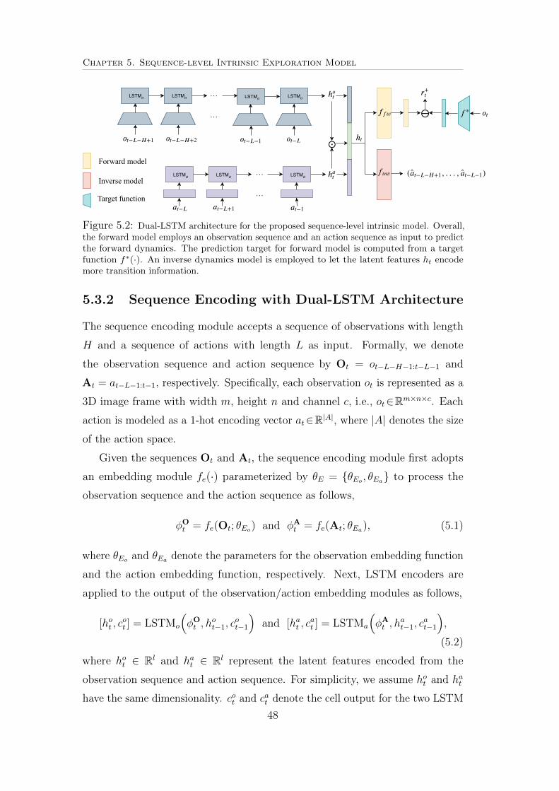
Chapter 5. Sequence-level Intrinsic Exploration Model
Targetfunction
Forwardmodel
LSTM
LSTM LSTM. . .
. . .
LSTM
LSTM
LSTM
Inversemodel
. . .
. . .
LSTM
Figure 5.2: Dual-LSTM architecture for the proposed sequence-level intrinsic model. Overall,the forward model employs an observation sequence and an action sequence as input to predictthe forward dynamics. The prediction target for forward model is computed from a targetfunction f⇤(·). An inverse dynamics model is employed to let the latent features ht encodemore transition information.
5.3.2 Sequence Encoding with Dual-LSTM Architecture
The sequence encoding module accepts a sequence of observations with length
H and a sequence of actions with length L as input. Formally, we denote
the observation sequence and action sequence by Ot = ot�L�H�1:t�L�1 and
At = at�L�1:t�1, respectively. Specifically, each observation ot is represented as a
3D image frame with width m, height n and channel c, i.e., ot2Rm⇥n⇥c. Each
action is modeled as a 1-hot encoding vector at2R|A|, where |A| denotes the size
of the action space.
Given the sequences Ot and At, the sequence encoding module first adopts
an embedding module fe(·) parameterized by ✓E = {✓Eo
, ✓Ea
} to process the
observation sequence and the action sequence as follows,
�Ot = fe(Ot; ✓E
o
) and �At = fe(At; ✓E
a
), (5.1)
where ✓Eo
and ✓Ea
denote the parameters for the observation embedding function
and the action embedding function, respectively. Next, LSTM encoders are
applied to the output of the observation/action embedding modules as follows,
[hot , c
ot ] = LSTMo
⇣�Ot , h
ot�1, c
ot�1
⌘and [ha
t , cat ] = LSTMa
⇣�At , h
at�1, c
at�1
⌘,
(5.2)
where hot 2 Rl and ha
t 2 Rl represent the latent features encoded from the
observation sequence and action sequence. For simplicity, we assume hot and ha
t
have the same dimensionality. cot and cat denote the cell output for the two LSTM
48
Chapter 5. Sequence-level Intrinsic Exploration Model
modules, which are stored for computing the sequence features in a recurrent
manner.
Next, the sequence features for the observation/action hot and ha
t are synthe-
sized to derive latent features ht which describe the past transitions:
hitrt = ho
t � hat and ht = [ho
t , hat , h
itrt ]. (5.3)
To compute ht, an multiplicative interaction is first performed over hot and ha
t ,
which results in hitrt and � denotes element-wise multiplication. Then ht is
derived by concatenating the multiplicative interaction feature hitrt with the
latent representations for the observation and action sequences, i.e., hot and ha
t .
The reason for generating ht in this way is that the prediction task over the
partial observation ot is related to both the local information conveyed in the two
sequences themselves (i.e., hot and ha
t ), as well as the collaborative information
derived via interacting the two sequence features in a form. The reason for
performing multiplicative interaction is that the advancement of such operation
has been validated in prior works [41, 79]. We demonstrate that generating ht in
the proposed form is e↵ective and crucial to derive a desirable policy learning
performance in the ablation study of the experiment section.
5.3.3 Computing Novelty from Prediction Error
The latent features ht are employed as input by a feedforward prediction function
to predict the forward dynamics:
t = ffw(ht; ✓F ) and ⇤t = f⇤(ot), (5.4)
where ffw(·) is the forward prediction function parameterized by ✓F , and t
denotes the prediction output. We use ⇤t to denote the prediction target, which
is computed from some target function f⇤(·). Within the proposed novelty
framework, the target function f⇤(·) could be derived in various forms, where the
common choices include the representation of ot at its original feature space, i.g.,
image pixels, and the learned embedding of ot, i.e., fe(·; ✓Eo
). Apart from the
conventional choices, in this work, we employ a target function computed from a
random network distillation model [72], which demonstrates great e�ciency in
distinguishing the novel states. Thus, f⇤(·) is represented by a fixed and randomly
49

Chapter 5. Sequence-level Intrinsic Exploration Model
initialized target network. Intuitively, it forms a random mapping from each input
observation to a point in a k-dimensional space, i.e., f⇤ : Rm⇥n⇥c ! Rk. Hence
the forward dynamics model is trained to distill the randomly drawn function
from the prior. The prediction error inferred from such a model is related to the
uncertainty quantification in predicting some constant zero function [80].
The novelty of a state is inferred from the uncertainty evaluated as the MSE
loss for the forward model. Formally, at step t, a novelty score or reward bonus
is computed in the following form:
r+(Ot,At) =�
2|| ⇤
t � t||2
2, (5.5)
where � � 0 is a hyperparameter to scale the reward bonus. The reward
bonus is issued to the agent in a step-wise manner. During the policy learning
process, the agent maximizes the sum over the external rewards and the intrinsic
rewards derived from the novelty model. Therefore, the overall reward term to
be maximized as will be shown in (5.8) is computed as rt = ret + r+t , where ret
denotes the external rewards from the environment.
5.3.4 Loss Functions for Model Training
The training of the forward dynamics model turns out to be a regression problem.
The optimization is conducted by minimizing the following loss:
Lfw( ⇤t , t) =
1
2|| ⇤
t � t||2
2. (5.6)
We additionally incorporate an inverse dynamics model finv over the latent
features ht to make them encode more abundant transition information. Given
the observation sequence Ot with length H, the inverse model is trained to
predict the H � 1 actions taken between the observations. Thus, the inverse
model is defined as:
finv�ht; ✓I
�=
H�1Y
i=1
p(at�L�i), (5.7)
where finv(·) denotes the inverse function parameterized by ✓I , and p(at�L�i)
denotes the action distribution output for time step t�L� i. The inverse model
is trained with a standard cross-entropy loss.
Overall, the forward loss and inverse loss are jointly optimized together with
the reinforcement learning objective, without any pretraining required. Moreover,
50

Chapter 5. Sequence-level Intrinsic Exploration Model
Spawn locationGoal
Sparse
Very sparse
Figure 5.3: The 3D navigation task domains adopted for empirical evaluation: (1)an example of partial observation frame from ViZDoom task; (2) the spawn/goallocation settings for ViZDoom tasks; (3/4) an example of partial observationframe from the apple-distractions/goal-exploration task in DeepMind Lab.
the parameters for the observation embedding module ✓Eo
could be shared with
the policy model. In summary, the compound objective function for deriving the
intrinsically motivated reinforcement learning policy becomes:
min✓E
,✓F
,✓I
,✓⇡
�Lfw( ⇤t , t) +
(1� �)H � 1
H�1X
i=1
Linv(at�L�i, at�L�i)� ⌘E⇡(�ot
;✓⇡
)[X
t
rt],
(5.8)
where ✓E, ✓F and ✓I are the parameters for the novelty model, ✓⇡ are the
parameters for the policy model, Linv(·) is the cross-entropy loss for the inverse
model, 0 � 1 is a weight to balance the loss for the forward and inverse
models, and ⌘ � 0 is the weight for the reinforcement learning loss.
5.4 Experiments
5.4.1 Experimental Setup
Task Domains For empirical evaluation, we adopt three 3D navigation tasks
with first-person view: 1) ‘DoomMyWayHome-v0 ’ from ViZDoom [81]; 2) ‘Stair-
way to Melon’ from DeepMind Lab [82]; 3) ‘Explore Goal Locations ’ from Deep-
Mind Lab. The experiments in ‘DoomMyWayHome-v0 ’ allow us to test the
algorithms in scenarios with varying degrees of reward sparsity. The experiments
in ‘Stairway to Melon’ allow us to test the algorithms in scenarios with reward
distractions. The experiments in ‘Explore Goal Locations’ allow us to test the
algorithms in scenarios with procedurally generated maze layout and random
goal locations.
51

Chapter 5. Sequence-level Intrinsic Exploration Model
Baseline Methods For fare comparison, we adopt ‘LSTM-A3C’ as the RL
algorithm for all the methods. In the experiments, we compare with the vanilla
‘LSTM-A3C’ as well as the following intrinsic exploration baselines: 1) the
Intrinsic Curiosity Module [38], denoted as ‘ICM’; 2) Episodic Curiosity through
reachability [76], denoted as ‘EC’; 3) the Random Network Distillation model,
denoted as ‘RND’. Our proposed Sequence-level Intrinsic Module is denoted as
‘SIM’. All the intrinsic exploration baselines adopt non-sequential inputs. The
baseline ‘EC’ is a memory-based algorithm and requires careful pretraining, so we
shift the corresponding learning curves by the budgets of pretraining frames (i.e.,
0.6M) in the results to be presented, following the original paper [76]. Except for
‘EC’, the exploration models in all the other baselines are jointly trained with
the policy model.
5.4.2 Evaluation with Varying Reward Sparsity
Our first empirical domain is a navigation task in the ‘DoomMyWayHome-v0 ’
scenario from ViZDoom. The task consists of a static maze layout and a fixed
goal location. At the start of each episode, the agent spawns from one of the
17 spawning locations, as shown in Figure 5.3. In this domain, we adopt three
di↵erent setups with varying degree of reward sparsity, i.e., dense, sparse, and
very sparse. Under the dense setting, the agent spawns at one randomly selected
location from the 17 locations and it is relatively easy to succeed in navigation.
Under the sparse and very sparse settings, the agent spawns at a fixed location
far away from the goal. The environment issues a positive reward of +1 to
the agent when reaching the goal. Otherwise, the rewards are 0. The episode
terminates when the agent reaches the goal location or the episode length exceeds
the time limit of 525 4-repeated steps.
We show the training curves measured in terms of navigation success ratio in
Figure 5.4. The results from Figure 5.4 depicts that as the rewards go sparser, the
navigation would become more challenging. The vanilla ‘LSTM-A3C’ algorithm
could not progress at all under the sparse and very sparse settings. ‘ICM’ could
not reach 100% success ratio under the sparse and very sparse settings, and so
does ‘EC’ under the very sparse setting. However, our proposed method could
consistently achieve 100% success ratio across all the tasks with varying reward
sparsity. The detailed convergence scores are shown in Table 5.1.
52

Chapter 5. Sequence-level Intrinsic Exploration Model
Figure 5.4: Learning curves measured in terms of the navigation success ratio inViZDoom. The figures are ordered as: 1) dense; 2) sparse; 3) very sparse. Werun each method for 6 times.
53

Chapter 5. Sequence-level Intrinsic Exploration Model
dense sparse very sparse
LSTM-A3C 100% 0.0% 0.0%ICM 100% 66.7% 68.6%EC 100% 100% 75.5%RND 100% 100% 100%SIM 100% 100% 100%
Table 5.1: Performance scores for the three task settings in ViZDoom evaluatedover 6 independent runs. Overall, only our approach and ’RND’ could convergeto 100% under all the settings.
Our proposed solution also demonstrates significant advantage in terms of
convergence speed. Though the reward sparsity varies, our method could quickly
reach 100% success ratio in all the scenarios. However, the convergence speeds
of ‘ICM’, ‘EC’ and ‘RND’ apparently degrade with sparser rewards. Also, we
notice that the memory-based method (i.e., ‘EC’) takes much longer time to
converge compared to the prediction-error based baselines ‘RND’ and ‘SIM’.
That is, the learning curves for those prediction-error based methods go up with
a much steeper ratio compared to the memory-based method. The reason is that
‘EC’ keeps a memory which is being updated at runtime to compute the novelty.
Therefore, the novelty score assigned for each state might be quite unstable.
Moreover, ‘EC’ requires a non-trivial task to pretrain the comparator module to
make it work.
Overall, our proposed method could converge to 100% success ratio on average
3.0x as fast as ‘ICM’ and 1.97x compared to ‘RND’. We show detailed convergence
statistics in Table 5.2.
LSTM-A3C ICM RND EC SIM (ours)
dense 7.13m 3.50m 1.86m >10m 1.50msparse >10m 6.01m 4.51m 6.45m 1.82mvery sparse >10m 6.93m 4.55m >10m 2.27m
Table 5.2: The approximated environment steps taken by each algorithm toreach its convergence standard under each task setting. Notably, our proposedalgorithm could achieve an average speed up of 2.89x compared to ‘ICM’, and1.90x compared to ‘RND’.
54

Chapter 5. Sequence-level Intrinsic Exploration Model
5.4.3 Evaluation with Varying Maze Layout and Goal Lo-cation
Our second empirical evaluation engages a more dynamic navigation task with
procedurally generated maze layout and randomly chosen goal locations. We
adopt the ‘Explore Goal Locations’ level script from DeepMind Lab. At the
start of each episode, the agent spawns at a random location and searches for a
randomly defined goal location within the time limit of 1350 4-repeated steps.
Each time the agent reaches the goal, it receives a reward of +10 and is spawned
into another random location to search for the next random goal. The maze
layout is procedurally generated at the start of each episode. This domain
challenges the algorithms to derive general navigation behavior instead of relying
on remembering the past trajectories.
Figure 5.5: Learning curves for the procedurally generated goal searching task inDeepMind Lab. We run each method for 5 times.
We show the results with an environment interaction budget of 2M 4-repeated
steps in Figure 5.5. As a result, the method without intrinsic novelty model
could only converge to an inferior performance around 10. Our proposed method
could score > 20 with less than 1M training steps, whereas ‘ICM’ and ‘RND’
take almost 2M steps to score above 20. This demonstrates that our proposed
algorithm could progress at a much faster speed compared to all the baselines
under the procedurally generated maze setting.
55

Chapter 5. Sequence-level Intrinsic Exploration Model
5.4.4 Evaluation with Reward Distractions
Our third empirical evaluation engages a cognitively complex task with reward
distraction. We adopt the ‘Stairway to Melon’ level script from DeepMind Lab.
In this task, the agent can follow either two corridors: one of them leads to a
dead end, but has multiple apples along the way, collecting which the agent
would receive a small positive reward of +1; the other corridor consists of one
lemon which gives the agent a negative reward of �1, but after passing the lemon,
there are stairs that lead to the navigation goal location upstairs indicated by a
melon. Collecting the melon makes the agent succeed in navigation and receive a
reward of +20. The episode terminates when the agent reaches the goal location
or the episode length exceeds the time limit of 525 4-repeated steps.
The results are shown in Figure 5.6. We show both the cumulative episode
reward and the success ratio for navigation. Due to the reward distractions,
the learning curves for each approach demonstrate instability with ubiquitous
glitches. The vanilla ‘LSTM-A3C’ could only converge to an inferior navigation
success ratio of < 50%, and all the other baselines progress slowly. Notably, our
proposed method could fast grasp the navigation behavior under the reward
distraction scenario, i.e., surpassing the standard of > 80% with less than 0.2M
environment interactions, which is at least 3x as fast as the compared baselines.
5.4.5 Ablation Study
In this section, we present the results for an ablation study under the very sparse
task in ViZDoom.
Impact of varying sequence length: We investigate the performance of our
proposed algorithm with varying observation/action sequence lengths. First,
we fix the observation sequence length to be 10 and set the action sequence
length from {1, 3, 6, 9}. From the results shown in Figure 5.7, we conclude that
our algorithm performs quite consistently with di↵erent action sequence lengths.
Overall, the algorithm appears to work well with a moderate action sequence
length of 6. Second, we fix the action sequence length to be 6 and vary the
observation sequence length from {3, 10, 20}. When the observation sequence is
too long, i.e., 20, the algorithm converges very slowly. Thus, we recommend a
moderate observation sequence length of 10 to be used.
56

Chapter 5. Sequence-level Intrinsic Exploration Model
Figure 5.6: Learning curves for ’Stairway to Melon’ task in DeepMind Lab.Up: cumulative episode reward; Down: navigation success ratio. We run eachmethod for 5 times.
Impact of ht: We demonstrate that modeling ht in the proposed form of (5.3)
is e�cient by comparing our method with the following two baseline models
of ht: 1) only using the interactive features hitrt , denoted by ‘SIM-itr’, and 2)
only using the concatenation of hot and ha
t , denoted by ‘SIM-concat’. From the
results shown in Figure 5.8, we find that both baseline methods converge to
inferior performance standard, i.e., the algorithm fail occasionally so that the
averaged curve could not converge to 100% success ratio. When using ht in the
proposed form, the algorithm could consistently converge to 100% success ratio.
This demonstrates that modeling ht in our proposed form is crucial for deriving
a desired policy learning performance.
57
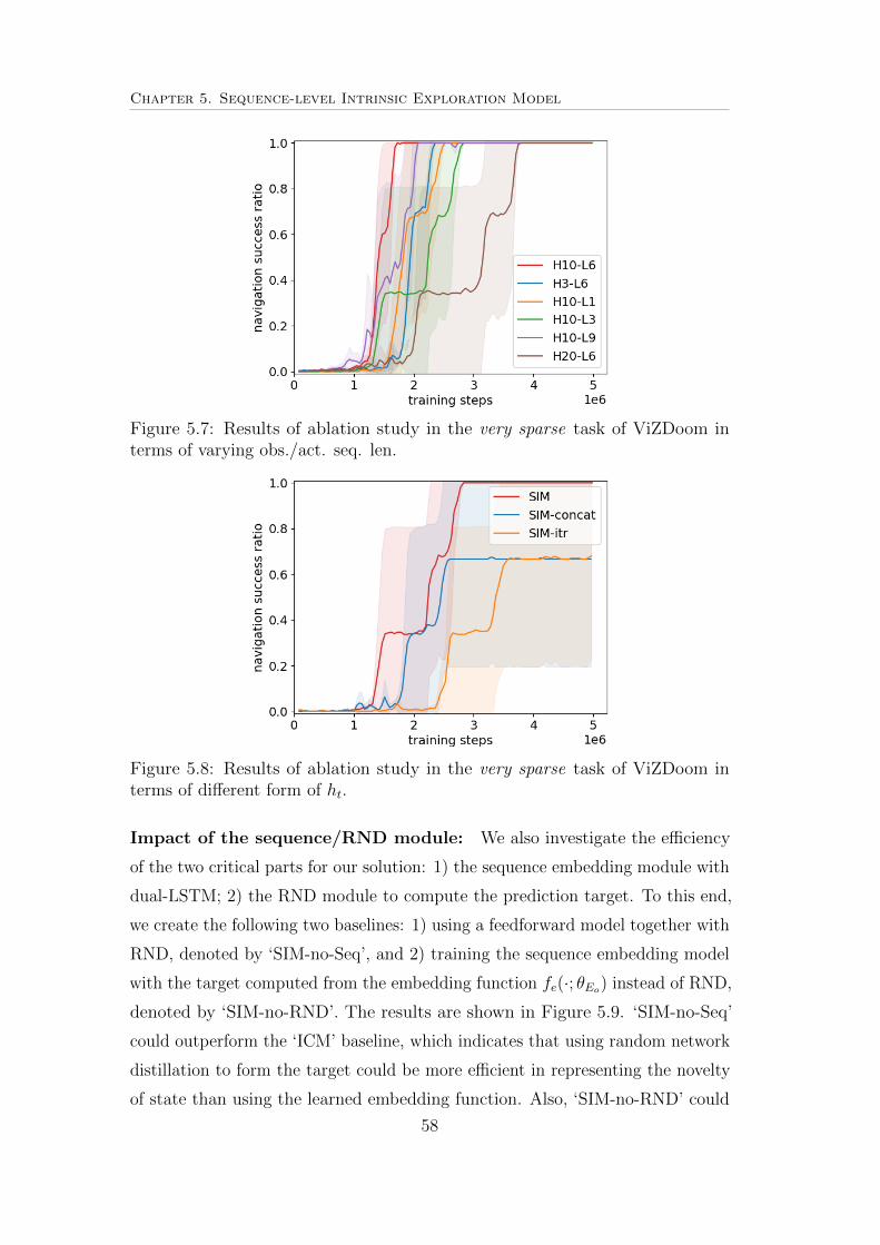
Chapter 5. Sequence-level Intrinsic Exploration Model
Figure 5.7: Results of ablation study in the very sparse task of ViZDoom interms of varying obs./act. seq. len.
Figure 5.8: Results of ablation study in the very sparse task of ViZDoom interms of di↵erent form of ht.
Impact of the sequence/RND module: We also investigate the e�ciency
of the two critical parts for our solution: 1) the sequence embedding module with
dual-LSTM; 2) the RND module to compute the prediction target. To this end,
we create the following two baselines: 1) using a feedforward model together with
RND, denoted by ‘SIM-no-Seq’, and 2) training the sequence embedding model
with the target computed from the embedding function fe(·; ✓Eo
) instead of RND,
denoted by ‘SIM-no-RND’. The results are shown in Figure 5.9. ‘SIM-no-Seq’
could outperform the ‘ICM’ baseline, which indicates that using random network
distillation to form the target could be more e�cient in representing the novelty
of state than using the learned embedding function. Also, ‘SIM-no-RND’ could
58

Chapter 5. Sequence-level Intrinsic Exploration Model
Figure 5.9: Results of ablation study in the very sparse task of ViZDoom interms of the impact of seq./RND module.
converge much faster than ’ICM’, which indicates that using the sequence-level
modeling of novelty is more e�cient than using flat concatenation of frames.
Overall, this study shows that using the sequence embedding model together
with the RND prediction target is critical for deriving desirable performance.
Impact of the inverse dynamics module: We also investigate the e�ciency
of engaging the proposed inverse dynamics prediction module. To this end, we
evaluate the performance of our model when turning o↵ the inverse dynamics pre-
diction, by using di↵erent action sequence. From the result shown in Figure 5.10,
we notice that when turning o↵ invserse dynamics, the model could not perform
as well as its original form. Moreover, with the longer action sequence length,
the impact of inverse dynamics would be more significant, i.e., the performance
of turning o↵ inverse dynamics with action sequence length 3 is much worse than
that of 1.
5.4.6 Evaluation on Atari Domains
We also investigate whether the proposed exploration algorithm could work in
MDP tasks with non-partial observation and/or with large action space. To this
end, we testify the proposed exploration algorithm with non-sequential baselines
of ICM and RND in two Atari 2600 games: ms-pacman and seaquest. The
two domains have action space with size 9 and 18, respectively. The learning
59

Chapter 5. Sequence-level Intrinsic Exploration Model
Figure 5.10: Results of ablation study in the very sparse task of ViZDoom interms of the impact of inverse dynamics module.
curves are presented in Figure 5.11. The result shows that our proposed method
works much better than ICM/RND in both tasks. It results in apparently
higher convergence score than the other two approaches. This indicates that our
algorithm demonstrates certain e�ciency in non-partial observable MDP like
Atari. Furthermore, it could handle the tasks with relatively large action space
with considerable e�ciency.
60

Chapter 5. Sequence-level Intrinsic Exploration Model
Figure 5.11: Result of using SIM and non-sequential baselines of ICM and RNDin two Atari 2600 games: ms-pacman and seaquest.
61
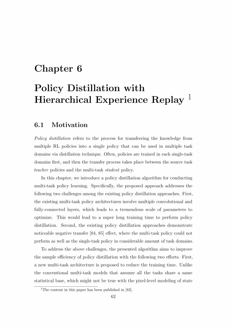
Chapter 6
Policy Distillation withHierarchical Experience Replay 1
6.1 Motivation
Policy distillation refers to the process for transferring the knowledge from
multiple RL policies into a single policy that can be used in multiple task
domains via distillation technique. Often, policies are trained in each single-task
domains first, and then the transfer process takes place between the source task
teacher policies and the multi-task student policy.
In this chapter, we introduce a policy distillation algorithm for conducting
multi-task policy learning. Specifically, the proposed approach addresses the
following two challenges among the existing policy distillation approaches. First,
the existing multi-task policy architectures involve multiple convolutional and
fully-connected layers, which leads to a tremendous scale of parameters to
optimize. This would lead to a super long training time to perform policy
distillation. Second, the existing policy distillation approaches demonstrate
noticeable negative transfer [84, 85] e↵ect, where the multi-task policy could not
perform as well as the single-task policy in considerable amount of task domains.
To address the above challenges, the presented algorithm aims to improve
the sample e�ciency of policy distillation with the following two e↵orts. First,
a new multi-task architecture is proposed to reduce the training time. Unlike
the conventional multi-task models that assume all the tasks share a same
statistical base, which might not be true with the pixel-level modeling of state
1The content in this paper has been published in [83].
62

Chapter 6. Policy Distillation with Hierarchical Experience Replay
space, our proposed architecture utilizes task-specific features transferred form
the single-task teacher models and only allows several fully connected layers to
be shared. This significantly increases the convergence speed and leads to a
multi-task policy with much less negative transfer e↵ect. Second, we propose
a hierarchical prioritized experience sampling approach to further increase the
sample e�ciency.
6.2 Notations
6.2.1 Deep Q-Networks
We define a Markov Decision Process (MDP) as a tuple (S,A,P , R, �), where
S represents a set of states, A represents a set of actions, P represents a
state transition probability matrix, where each entry P(s0|s, a) denotes the
probability for transiting to s0 from state s after taking action a, R is a reward
function mapping each state-action pair to a real-valued reward in R, and
�2 [0, 1] is a discount factor. The agent behavior in an MDP is represented by
a policy ⇡, where the value ⇡(a|s) represents the probability of taking action a
at state s. The value of Q-function Q(s, a) represents the expected cumulative
future rewards received after taking action a at state s following policy ⇡, i.e.,
Q(s, a) = EhPT
t=0 �trt|s0=s, a0=a
i, where T denotes a finite horizon and rt
denotes the reward received by the agent at time t. Based on the Q-function,
the state-value function could be defined as:
V (s) = maxa
Q(s, a). (6.1)
The optimal Q-function Q⇤(s, a) is the maximum Q-function over all policies. It
can be decomposed using the Bellman equation in the following manner,
Q⇤(s, a) = Es0
hr + �max
a0Q⇤(s0, a0|s, a)
i. (6.2)
Once the optimal Q-function is learned, we could derive the optimal policyfrom the learned action-value function. To learn the Q-function, the DQNalgorithm [14] uses a deep neural network to approximate the Q-function, whichis parameterized by ✓ as Q(s, a; ✓). The deep neural network function is trainedby minimizing the following loss function in an iterative manner,
L(✓i) = Es,a[(r + �maxa0
Q(s0, a0; ✓i�1)�Q(s, a; ✓i))2], (6.3)
63

Chapter 6. Policy Distillation with Hierarchical Experience Replay
where ✓i are the parameters for the Q-function from the i-th iteration.
During training, DQN adopts experience replay [86] techniques to break
the strong correlations between consecutive state inputs. At each time-step t,
the agent receives an experience tuple defined as et = {st, at, rt, st+1}, wherest is the observed state at time t, at is the action taken at time t, rt is the
reward received from the environment at t, and st+1 is the next state observed
by agent after after taking at at st. The recent experiences {e1, ..., eN} are stored
to construct a replay memory D, where N is the memory size. During policy
training, experiences are sampled from the replay memory to update the network
parameters.
6.2.2 Policy Distillation
Policy distillation transfers the knowledge learned by one or several Q-network(s)
(denoted as teacher) to a single multi-task Q-network (denoted as student) via
supervised regression. When transferring the knowledge, instead of using the
loss function as shown in (6.3) to optimize the student Q-network parameters,
the process minimizes the distribution divergence between teacher prediction
and student prediction.
Formally, we introduce the policy distillation setting as follows. Suppose there
are a set of m source tasks, denoted as S1, ..., Sm. Each of the source domains
has a trained a teacher policy, denoted as QTi
, where i=1, ...,m. The goal is to
train a multi-task student Q-network model, denoted by QS. During training,
each task domain Si stores its generated experience in a own replay memory
D(i) = {e(i)k ,q(i)k }, where e(i)k denotes the k-th experience in D(i), and q(i)
k denotes
the corresponding vector of Q-values over output actions generated by QTi
. The
values q(i)k provided by the teacher model serves as a regression target for the
student Q-network. Instead of matching the exact Q-values, previous research
has revealed that optimizing the student Q-network with the KL-divergence
between the output distribution of student model and the teacher Q-networks
model turns out to be more e↵ective [53]. Thus, the loss function for policy
distillation to optimize the parameters ✓S of the multi-task student Q-network is
defined in the following manner:
LKL
⇣D(i)
k , ✓S⌘= f
q(i)k
⌧
!· ln
0
@f⇣q(i)k /⌧
⌘
f⇣q(S)k
⌘
1
A , (6.4)
64
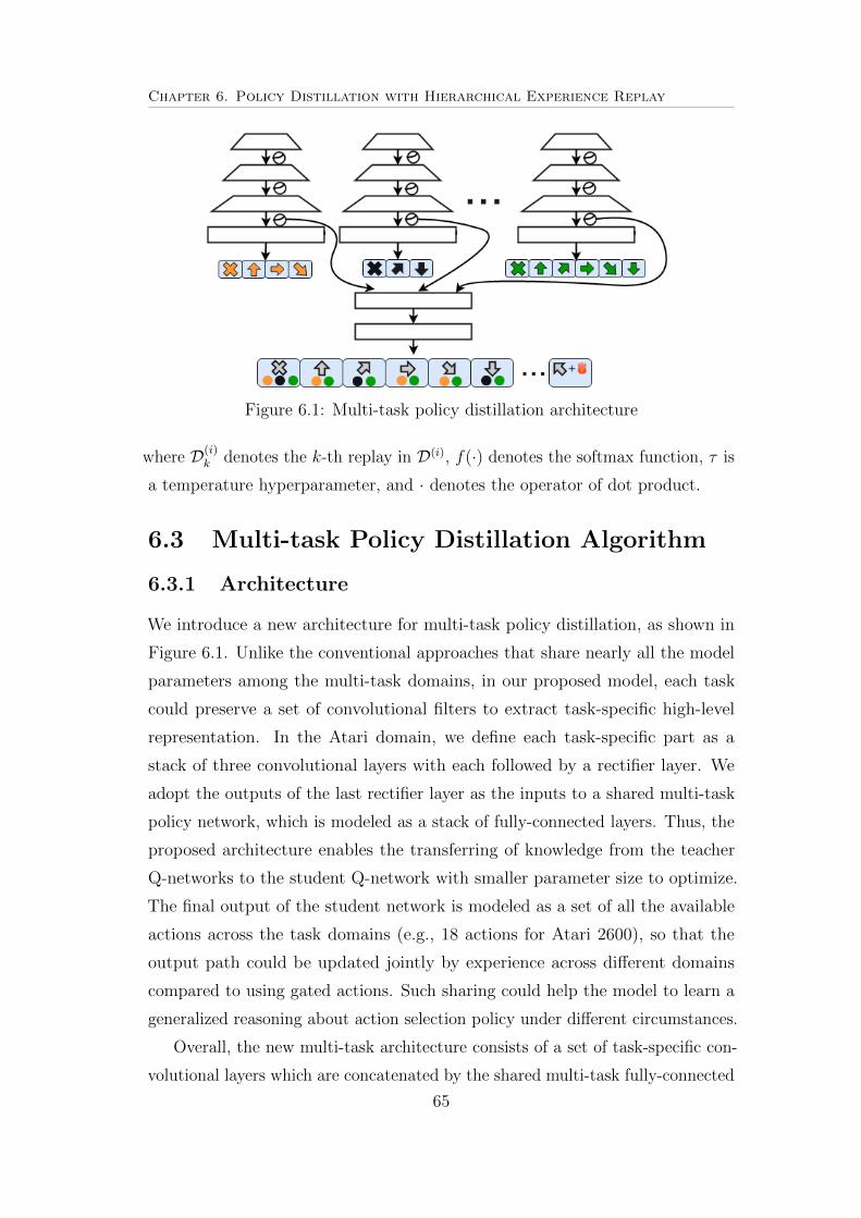
Chapter 6. Policy Distillation with Hierarchical Experience Replay
Figure 6.1: Multi-task policy distillation architecture
where D(i)k denotes the k-th replay in D(i), f(·) denotes the softmax function, ⌧ is
a temperature hyperparameter, and · denotes the operator of dot product.
6.3 Multi-task Policy Distillation Algorithm
6.3.1 Architecture
We introduce a new architecture for multi-task policy distillation, as shown in
Figure 6.1. Unlike the conventional approaches that share nearly all the model
parameters among the multi-task domains, in our proposed model, each task
could preserve a set of convolutional filters to extract task-specific high-level
representation. In the Atari domain, we define each task-specific part as a
stack of three convolutional layers with each followed by a rectifier layer. We
adopt the outputs of the last rectifier layer as the inputs to a shared multi-task
policy network, which is modeled as a stack of fully-connected layers. Thus, the
proposed architecture enables the transferring of knowledge from the teacher
Q-networks to the student Q-network with smaller parameter size to optimize.
The final output of the student network is modeled as a set of all the available
actions across the task domains (e.g., 18 actions for Atari 2600), so that the
output path could be updated jointly by experience across di↵erent domains
compared to using gated actions. Such sharing could help the model to learn a
generalized reasoning about action selection policy under di↵erent circumstances.
Overall, the new multi-task architecture consists of a set of task-specific con-
volutional layers which are concatenated by the shared multi-task fully-connected
65

Chapter 6. Policy Distillation with Hierarchical Experience Replay
layers. Under the teacher-student transfer learning setting, the parameters for
the task-specific parts could be derived conveniently from the corresponding
single-task teachers which are trained beforehand. The parameters for the multi-
task layers are randomly initialized and trained from scratch. The proposed
work assumes the task domains do not completely share the static base when
considering their pixel-level input space. Thus, considering the low-level state
representation is often quite task-specific, utilizing the task-specific features
would help the multi-task training to avoid negative transfer e↵ect. Meanwhile,
such modeling of network architecture would result in a significantly reduced
amount of trainable parameters so as to improve the time e�ciency for policy
distillation.
6.3.2 Hierarchical Prioritized Experience Replay
To further improve the time e�ciency, we introduce a new sampling approach
to select experience from the multiple source domains during the multi-task
training. The new sampling approach adopts a hierarchical sampling structure
and is therefore termed as hierarchical prioritized replay.
The design of the proposed hierarchical experience sampling approach is
motivated by of DQN’s replay memory and the prioritized experience replay
mechanism proposed to train the DQN [70] (at single-task domain). When
performing prioritized experience replay to train a standard DQN, we do not
perform uniform sampling over the experiences in the replay bu↵er. Instead, we
store the generated experiences with importance sampling weight to a replay
memory first, and then sample them based on their importance weight.
Sampling the experience with advanced strategy is crucial for the policy
training, since the experiences stored at the replay memory would form a distri-
bution. For some task domains, such distribution would vary a lot as the training
progress, since the output distribution of the policy keeps changing. One typical
example with such property is the game Breakout. In this game, at the initial
training phase, DQN would not visit the state shown in Figure 6.2 (left), unless
the RL agent has acquired the ability to dig a tunnel after considerable amount of
training. We also demonstrate histograms over the state distributions generated
by three Breakout policy networks in Figure 6.2 (right). The three policies are
66
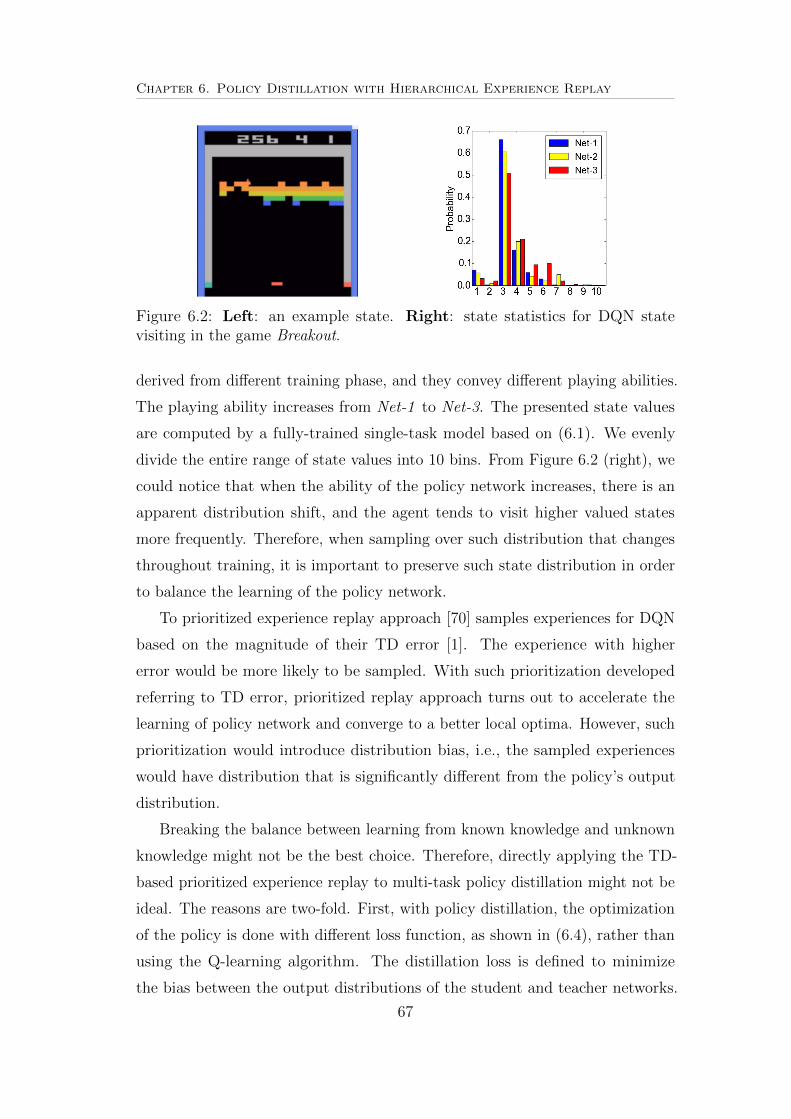
Chapter 6. Policy Distillation with Hierarchical Experience Replay
Figure 6.2: Left: an example state. Right: state statistics for DQN statevisiting in the game Breakout.
derived from di↵erent training phase, and they convey di↵erent playing abilities.
The playing ability increases from Net-1 to Net-3. The presented state values
are computed by a fully-trained single-task model based on (6.1). We evenly
divide the entire range of state values into 10 bins. From Figure 6.2 (right), we
could notice that when the ability of the policy network increases, there is an
apparent distribution shift, and the agent tends to visit higher valued states
more frequently. Therefore, when sampling over such distribution that changes
throughout training, it is important to preserve such state distribution in order
to balance the learning of the policy network.
To prioritized experience replay approach [70] samples experiences for DQN
based on the magnitude of their TD error [1]. The experience with higher
error would be more likely to be sampled. With such prioritization developed
referring to TD error, prioritized replay approach turns out to accelerate the
learning of policy network and converge to a better local optima. However, such
prioritization would introduce distribution bias, i.e., the sampled experiences
would have distribution that is significantly di↵erent from the policy’s output
distribution.
Breaking the balance between learning from known knowledge and unknown
knowledge might not be the best choice. Therefore, directly applying the TD-
based prioritized experience replay to multi-task policy distillation might not be
ideal. The reasons are two-fold. First, with policy distillation, the optimization
of the policy is done with di↵erent loss function, as shown in (6.4), rather than
using the Q-learning algorithm. The distillation loss is defined to minimize
the bias between the output distributions of the student and teacher networks.
67

Chapter 6. Policy Distillation with Hierarchical Experience Replay
Thus, the prioritization for policy distillation requires for a new scheme other
than TD-loss. Second, the experience sampled from each task domains following
prioritized experience replay technique would not be representative to preserve
the global population of experiences for the task domains.
We propose hierarchical prioritized experience technique to address the above
mentioned issues. In our proposed approach, sampling is performed in a hier-
archical manner as follows: it determines which part from the distribution to
sample, followed by which experience from that part to sample. To facilitate such
hierarchical structure, we define a hierarchical structure for the replay memory.
Specifically, each replay memory is divided into several partitions, and each
partition stores the experiences from a certain part of the state distribution.
We evaluate the state distribution based on the state value, which could be
predicted by the teacher networks. Within each partition, there is a priority
queue and the experiences are stored in a prioritized manner. During sampling,
the high-level sampling of partitions is done uniformly. This mechanism would
make the sampled experiences preserve the global state visiting distribution of the
policy model. When sampling experience from a specific partition, importance
sampling is adopted and the experiences are sampled according their priorities.
6.3.2.1 Uniform Sampling on Partitions
The high-level sampling determines a partition to sample. To this end, we
propose a partition assignment mechanism based on the state distribution. For
each task Si, we compute a state visiting distribution based on the state values
for the experiences. The state values could be predicted by the teacher network
QTi
following (6.1). We evaluate the boundary for each state distribution by
collecting some experience samples by the teacher network in each problem
domain, which is denoted as [V (i)min, V
(i)max]. Then the derived state distribution
range is evenly divided into p partitions, {[V (i)1 , V (i)
2 ], (V (i)2 , V (i)
3 ], ...(V (i)p , V (i)
p+1]}.Each partition consists of a prioritized memory queue to store the experiences.
Therefore, for each task domain Si, there would be p prioritized queues, with
the j-th queue storing the experience samples whose state values fall into the
range (V (i)j , V (i)
j+1].
The uniform sampling probability for partition selection is computed in the
following manner. At run-time, we keep track of the number of experiences that
68

Chapter 6. Policy Distillation with Hierarchical Experience Replay
have been assigned to a specific partition j for each task Si within a time window,
denoted by N (i)j . Then the probability for partition j to be selected under task
domain Si is computed as:
P (i)j =
N (i)jPp
k=1 N(i)k
. (6.5)
6.3.2.2 Prioritization within Each Partition
After selecting a partition for a task domain, e.g., partition j is selected for task
Si, we would sample a specific experience within that partition in prioritized
manner. To facilitate the policy distillation, we define a prioritization scheme
for the experiences in each partition based on the absolute gradient value of the
KL-divergence loss between the output distributions of the student network QS
and the teacher network QTi
w.r.t. q(S)j[k]
:
|�(i)j[k]| = 1
|ATi
|
������f
0
@q(i)j[k]
⌧
1
A� f⇣q(S)j[k]
⌘������1
, (6.6)
where |ATi
| is the number of actions for the i-th source task domain, j[k] is the
index of the k-th experience from partition j, and |�(i)j[k]| is the priority weight
assigned to that experience. Within the j-th partition for task domain Si, the
probability for an experience k to be selected is defined as:
P (i)j[k]
=
⇣�(i)j (k)
⌘↵
PN(i)j
t=1
⇣�(i)j (t)
⌘↵ , (6.7)
where �(i)j (k) = 1
rank(i)j
(k)with rank(i)j (k) denotes the position of ranking for
experience k in partition j which is determined by |�(i)j[k]| in descending order,
and ↵ is a scaling factor. The reason for using the ranking position instead of
proportion of its absolute gradient value to define the probabilities for experiences
is that prioritization with the rank-based information could result in more robust
update for importance sampling [70].
6.3.2.3 Bias Correction via Importance Sampling
With the proposed hierarchical sampling approach, the overall probability for the
experience k in partition j of the replay memory D(i) to be sampled is defined in
69

Chapter 6. Policy Distillation with Hierarchical Experience Replay
the following manner,
P (i)j (k) = P (i)
j ⇥ P (i)j[k]
. (6.8)
Since the sampling on particular experiences within a partition still preserves
prioritization property, as a result, the overall sampling would introduce bias
to the optimization of the student network parameters. Thus, we compute the
importance sampling weights as follows to conduct bias correction over each
sampled experience,
w(i)j (k) =
0
@1P
p
t=1 N(i)t
P (i)j ⇥ P (i)
j[k]
1
A�
=
0
@ 1
N (i)j
⇥ 1
P (i)j[k]
1
A�
, (6.9)
where � is a scaling factor. For stability reason, the weights are normalized by
dividing maxk,j
w(i)j (k) from the mini-batch, denoted by w(i)
j (k). Thus, the final
gradient used for updating the parameters with hierarchical prioritized sampling
is derived as,
w(i)j (k)⇥�(i)j[k]
. (6.10)
In summary, with the proposed hierarchical prioritized sampling approach,
we first perform uniform sampling over the partitions to make the sampled
experiences preserve a global distribution generated by the updated policy. Then
we prioritize the experiences in each partition by utilizing the gradient information
for policy distillation to select more meaningful data to update the network.
The above mentioned mechanism would require a trained teacher network to
compute state value for each experience. But since policy distillation naturally
falls into a student-teacher architecture to engage well trained teacher models in
each task domain, we don’t consider the requirement for teacher networks as a
big overhead for our method.
6.4 Experimental Evaluation
6.4.1 Task Domains
To evaluate the proposed multi-task network architecture, we create a multi-task
domain which consists of 10 Atari games:
70

Chapter 6. Policy Distillation with Hierarchical Experience Replay
• Beamrider : the player controls a beamrider ship to clear the alien craft
from Restrictor Shield, which is a large alien shield placed above earth’s
atmosphere. To clear a sector, the player needs to first destroy fifteen
enemy ships and then a sentinel ship will appear, which could be destroyed
using torpedo. There are distinct ways to destroy di↵erent type of ships.
The action space consists of 10 actions: {no-op, fire, up, right, left, right,upright, upleft, rightfire, leftfire}.
• Breakout : a ball-and-paddle game where a ball bounces in the space and
the player moves the paddle in its horizontal position to avoid the ball
from dropping out of the paddle. The agent loses one life if the paddle fails
to collect the ball. The agent is rewarded when the ball hits bricks. The
action space consists of 4 actions: {no-op, fire, left, right}.
• Enduro: a racing game where the player controls a racing car on a long-
distance endurance lace. The player needs to pass certain cars each day to
continue racing for the following day. The visibility, whether and tra�c
would change throughout the racing. The action space consists of 9 actions:
{no-op, fire, right, left, down, downright, downleft, rightfire, leftfire}.
• Freeway : a chicken-crossing-high-way game where the player controls a
chicken to cross a ten lane high-way. The high-way is filled with moving
tra�c. The agent is rewarded if it could reaches the other side of the
high-way. It would lose life if hit by tra�c. The action space consists of
three actions: {no-op, up, down}.
• Ms-Pacman: the player controls an agent to traverse through an enclosed
2D maze. The objective of the game is to eat all of the pellets placed in the
maze while avoiding four colored ghosts. The pellets are placed at static
locations whereas the ghosts could move. There is a specific type of pellets
that is large and flashing. If eaten by player, the ghosts would turn blue
and flee and the player could consume the ghosts for a short period to earn
bonus points. The action space consists of 9 actions: {no-op, up, right, left,down, upright, upleft, downright, downleft}.
71

Chapter 6. Policy Distillation with Hierarchical Experience Replay
• Pong : a sport game simulating table tennis. The player controls a paddle
to move in vertical direction, placed at the left or right side of the screen.
The paddle is expected to hit the ball back and forth. The goal is to earn
11 points before the opponent. The action space consists of six actions:
{no-op, fire, right, left, rightfire, leftfire}.
• Q-bert :the game is to use isometric graphics puzzle elements formed in a
shape of pyramid. The objective of the game is to control a Q-bert agent to
change the color of every cube in the pyramid to create a pseudo-3D e↵ect.
To this end, the agent hops on top of the cube while avoiding obstacles and
enemies. The action space consists of six actions: {no-op, fire, up, right,left, down}.
• Seaquest : the player controls a submarine to shoot at enemies and rescue
divers. The enemies would shoot missiles at the player’s submarine. The
submarine has a limited amount of oxygen, so that the player needs to
surface often to replenish oxygen. The action space consists of the full set
of 18 Atari 2600 actions.
• Space Invaders : a fixed shooter game where the player controls a laser
cannon to move horizontally at the bottom of the screen and fire at
descending aliens. The player’s cannon is protected by several defense
bunkers. The game is rewarded when the player shoots an alien. As more
aliens are shot, the movement of the alien would speed up. If the alien reach
the bottom, the alien invasion is successful and the episode terminates. The
action space consists of 6 actions: {no-op, left, right, fire, leftfire, rightfire}.
• RiverRaid : the player controls a jet with a top-down view. The jet can
move left or right and being accelerated or decelerated. The jet clashes
if it collides with the riverbank or enemy craft. It also has limited fuel.
Reward is earned when the player shoots enemy tankers, helicopters, jets,
fuel depots and bridges. The action space consists of the full set of 18 Atari
2600 actions.
To evaluate the hierarchical prioritized experience sampling approach, we
selected 4 games from our multi-task domain with 10 tasks, which are Breakout,
Freeway, Pong and Q-bert.
72

Chapter 6. Policy Distillation with Hierarchical Experience Replay
6.4.2 Experiment Setting
We adopt the same network architecture as DQN [14] to train the single-task
teacher DQNs in each domain. For the multi-task student network for our
approach, the architecture is shown in Figure 6.1. We utilize the convolutional
layers from the trained teacher models to form the task-specific high-level features.
The high-level features have a dimension size of 3,136. Moreover, the student
network has two fully connected layers with each consisting of 1,028 and 512
neurons. The output layer consists of 18 units, with each output representing
one control action in Atari games. Each game adopts a subset of actions. During
training, we mask the unused actions and di↵erent games might share the same
outputs as long as they contain the corresponding control actions.
We keep a separate replay memory to store experience samples for each
task domain. The stored experiences are generated by the student Q-network
following an ✏-greedy strategy . The value for ✏ linearly decays from 1 to 0.1
within first 1 million steps. At each step, a new experience is generated for
each game domain. The student performs one mini-batch update by sampling
experience from each teacher’s replay memory at every 4 steps. For hierarchical
prioritized experience sampling, we define the number of partitions for each task
domain to be 5. Each partition stores up to 200,000 experience samples. When
performing uniform sampling, the replay memory capacity is set to be 500,000.
Overall, the total experience size for hierarchical experience replay is greater
than uniform sampling. But we claim that this size has neutral e↵ect on the
learning performance.
During the training, evaluation is performed once after every 25,000 updates
of mini-batch steps on each task. To avoid the agent to memorize the steps, a
random number of null operations (up to 30) are generated at the start of each
episode. Each evaluation plays 100,000 control steps, by following a behavior
policy of ✏-greedy strategy with ✏ set as 0.05 (a default setting for evaluating
deep RL models [53]).
6.4.3 Evaluation on Multi-task Architecture
We compare the proposed multi-task network architecture with the following two
baselines. The first baseline is proposed by [53], denoted by DIST. It consists of a
73

Chapter 6. Policy Distillation with Hierarchical Experience Replay
set of shared convolutional layers concatenated by a task-specific fully-connected
layer and an output layer. The second baseline is the Actor-Mimic Network
(AMN) proposed by [54]. It shares all the convolutional, fully-connected and
output layers.
During evaluation, we create and train a policy network according to each
architecture on the multi-task domain that consists of 10 tasks. To make a fair
comparison, we adopt uniform sampling for all approaches and use the same set
of teacher networks. For optimization, RMSProp algorithm [87] is adopted. Each
approach is run with three random seeds. The average result is reported. We
train the networks under each architecture for up to 4 million steps. Note that a
single optimization step for DIST takes the longest time. With modern GPUs,
the reported results for DIST consumed approximately 250 hours of training
time without taking into account of the evaluation time.
We show the performance for the best models for each approach in the 10
task domains is shown in Table 6.1. We report the performance for the multi-task
networks as the percentage of the corresponding teacher network’s score. We
could notice that our proposed architecture could stably yield to performance
at least as good as the corresponding teacher models for all the task domains.
This demonstrates that our proposed method consists of considerable tolerance
towards negative transfer. However, for DIST, we could find its performance falls
Teacher DIST AMN Proposed(score) (% of teacher)
Beamrider 6510.47 62.7 60.3 104.5Breakout 309.17 73.9 91.4 106.2Enduro 597.00 104.7 103.9 115.2Freeway 28.20 99.9 99.3 100.4
Ms.Pacman 2192.35 103.8 105.0 102.6Pong 19.68 98.1 97.2 100.5Q-bert 4033.41 102.4 101.4 103.9Seaquest 702.06 87.8 87.9 100.2
Space Invaders 1146.62 96.0 92.7 103.3River Raid 7305.14 94.8 95.4 101.2
Geometric Mean 92.4 93.5 103.8
Table 6.1: Performance scores for policy networks with di↵erent architectures ineach game domain.
74

Chapter 6. Policy Distillation with Hierarchical Experience Replay
far behind the single-task models (<75%) in games Beamrider and Breakout.
Also, AMN could not learn well in the task Beamrider, compared to its single-task
teacher models, either. Moreover, the results in Table 6.1 demonstrate that the
knowledge sharing among multiple tasks with our proposed architecture could
bring noticeable positive transfer e↵ect in the task Enduro. Our model results in
a performance increase of >15%.
We also show our proposed architecture could lead to significant advantage
in terms of time e�ciency to train the multi-task policy. Four out of the 10
games, Breakout, Enduro, River Raid and Space Invaders, take longer time to
train than others, since our method converges within 1 million mini-batch steps
in all other domains but those four. We present the learning curves on those
four games for di↵erent architectures in Figure 6.3. The result shows that our
6.3.a: Breakout 6.3.b: Enduro
6.3.c: River Raid 6.3.d: Space Invaders
Figure 6.3: Learning curves for di↵erent architectures on the 4 games thatrequires long time to converge.
75

Chapter 6. Policy Distillation with Hierarchical Experience Replay
proposed architecture could converge significantly faster than the other two
architectures even in those games which require for long training time. For all of
the 10 games, our method could converge within 1.5 million steps, while the two
baseline architectures would require at least 2.5 million steps to get all games
converge.
6.4.4 Evaluation on Hierarchical Prioritized Replay
We evaluate the e�ciency of the proposed hierarchical prioritized sampling
approach, denoted by H-PR, by comparing it with two other sampling approaches:
uniform sampling, denoted by Uniform, and prioritized replay with rank-based
mechanism [70], denoted by PR. The four task domains are selected so that we
could demonstrate the impact of sampling on both slow convergence domains
6.4.a: Breakout 6.4.b: Freeway
6.4.c: Pong 6.4.d: Q-bert
Figure 6.4: Learning curves for the multi-task policy networks with di↵erentsampling approaches.
76

Chapter 6. Policy Distillation with Hierarchical Experience Replay
(Breakout and Q-bert) and fast convergence domains (Freeway and Pong). Note
that when p=1, H-PR is reduced to as PR, and when we set p to be the size
of the replay memory, H-PR could be reduced to as Uniform. All sampling
approaches are implemented under our proposed multi-task architecture.
We show the performance of the policy networks trained by adopting di↵erent
sampling approaches in Figure 6.4. Two of the games, Freeway and Pong, are
rather easy to train. In these two games, H-PR does not show significant advan-
tage than the other baselines. However, for Breakout and Q-bert which converges
rather slowly, the advantage for H-PR becomes more obvious. Especially for the
game Breakout, where the overall state visiting distribution varies at great scale
during the policy learning stage, the e↵ect of H-PR is more significant. Overall,
in Breakout and Q-bert, our proposed approach only takes approximately 50% of
the steps taken by the Uniform baseline to reach a performance level of scoring
over 300 and 4,000 respectively.
6.4.4.1 Sensitivity of Partition Size Parameter
We present a study on investigating the impact of the partition size parameter, p,
on the learning performance of the policy distillation. To this end, we implement
H-PR on our proposed network architecture with a varying partition size from
{5, 10, 15}. The results are presented in Figure 6.5. We notice that when we set
p to be di↵erent values, H-PR demonstrates consistent acceleration on the policy
learning. This indicates the partition size parameter has a moderate impact
on our proposed method. However, considering that when the capacity of each
partition remains to be the same, the memory consumption would increase with
the increased partition size, we recommend 5 to be used as the default partition
size.
77
Chapter 6. Policy Distillation with Hierarchical Experience Replay
Figure 6.5: Learning curves for H-PR with di↵erent partition sizes for Breakoutand Q-bert respectively.
78

Chapter 7
Zero-Shot Policy Transfer withAdversarial Training
7.1 Motivation
Transfer learning develops the ability of learning algorithms to exploit the
commonalities between related tasks so that knowledge learned from some source
task domain(s) could e�ciently help the learning in the target task domain [88, 84].
When adopted in reinforcement learning (RL) scenarios, it enables the intelligent
agent to utilize the skills acquired by some source task policies to solve new
problems in the target task domains. In this chapter, we present an algorithm to
improve the policy generalization ability of deep RL agents under a challenging
setting, where data from the target domain is strictly inaccessible for the learning
algorithm. This problem is also referred to as zero-shot policy generalization,
where the RL policy is evaluated on a disjointed set of target domain from the
source domains, with no further fine-tuning performed on the target domain
data [89, 63].
Specifically, we tackle the zero-shot policy transfer problems with setting
same as [63], where there are a small number of task distinctive factors resulting
in shift to input state distribution, among which some are domain invariant
and critical to policy learning, and the others are task specific and irrelevant
to policy learning. E.g., learning to pick up certain type of objects placed in a
green room (i.e., source domain) and generalizing the policy to pick up the same
objects in a pink room (i.e., target domain). To tackle such problems, e�ciently
minimizing the e↵ect of task irrelevant factors (i.e., room color) while retaining the
domain invariant factors (e.g., object type to be picked up) could be a promising
79

Chapter 7. Zero-Shot Policy Transfer with Adversarial Training
solution to learn generalizable policy. In this work, we improve upon the existing
unsupervised feature learning approach [63]. Instead of separately encoding
domain invariant features with task specific/irrelevant ones, our objective is to
try best to eliminate the task irrelevant features and derive only domain invariant
ones for training generalizable policy. To this end, we formulate a novel solution
that utilizes the readily available task distinctive factors as labels to train a
variational autoencoder. Also, we propose an adversarial training mechanism to
e�ciently align the latent feature space.
7.2 Multi-Stage Zero-Shot Policy Transfer Set-ting
LetDS(SS,AS, TS,RS) andDT (ST ,AT , TT ,RT ) be the source-domain and target-
domain MDPs respectively. In this paper, we tackle the zero-shot policy transfer
problems with the same setting as [63], where the distinction of domains is
introduced by the shift in input state representation, i.e., SS 6= ST . The source
domain DS and target domain DT have the structural similar action set A,
reward function R and transition function T .
Formally, we define the shift in input state representation to be controlled
by a set of task distinctive generating factors fk (for domain k), which are
discrete. In practical scenarios, we assume such task distinctive factors fk
would have a very small size since the source and target domains would share
significant commonality. For fk, we further classify them into two types: the
task-irrelevant/domain-specific factor fk and the task-relevant/domain-invariant
factor fk� . To learn transferable representation, our overall objective is to eliminate
information corresponding to task-irrelevant/domain-specific factor (f ) while
e�ciently preserving information on task-relevant/domain-invariant factor (f�).
Identifying such task distinctive generating factors fk is handy, since the
tasks in transfer learning setting are expected to share significant commonality.
For instance, in one of our experimental domain DeepMind Lab, we have four
domains as shown in Figure 7.1, with each characterized by a conjunction of
room color and object-set type. Thus we define fk as: fk = {fR, fO}, wherefR 2 {Green, P ink} corresponds to room color factor which is task-irrelevant,
80

Chapter 7. Zero-Shot Policy Transfer with Adversarial Training
Room
1
Room
2
Object
Set
Set B
(R1, OA)
Set A
Room
target domain (R2, OA)
(R1, OB)
Figure 7.1: Zero-shot setting in DeepMind Lab (room color (fR) is task-irrelevant factor and object-set type (fO) is task-relevant factor). The tasks beingconsidered are object pick-up tasks with partial observation. There are two typesof objects placed in one room, where picking up one type of object would begiven positive reward whereas the other type resulting in negative reward. Theagent is restricted to performing pick up task within a specified duration.
and fO 2 {Hat/Can,Balloon/Cake} corresponds to object-set factor which is
task-relevant. So we have f = {fR} and f� = {fO}. In our work, we utilize such
readily available labels of fk to align the state space representation.
In this work, we adopt a multi-stage policy learning [63, 90]. In contrast
to the conventional end-to-end deep RL methods which directly learn a policy
⇡ : sko ! A over the raw observation sko , multi-stage policy learning first takes
a feature learning stage to learn a universal function F : sko ! sz from the
auxiliary domains, to map each low-level state observation sko to a high-level
latent representation sz. Then a policy learning stage is taken over the source
domains, where a policy function is trained over the latent state representation
⇡ : sz ! A. For the example in Figure 7.1, we use 3 domains as auxiliary
domains to train feature learning model, and one domain with a disjoint set of
generating factors from the auxiliary and source domains as zero-shot target
domain. For source domains, we adopt two settings: 1) use the 3 auxiliary
domains as source; 2) only use one with same domain invariant label from target
domain as source.
Note that with the above setting, our work introduces a much more challenging
zero-shot transfer task than the related work [63]. First, more auxiliary domains
81

Chapter 7. Zero-Shot Policy Transfer with Adversarial Training
for feature learning are used in [63], and their auxiliary domains include the
conjunction of each single target domain object type with the target domain
room color (e.g., the feature learning model sees a hat or can in a pink room).
However, in our setting, such conjunction is neither included in auxiliary domains
nor source domains, which makes the zero-shot setting more challenging. Second,
we further restrict the policy to be trained in only one source domain (as one of
our settings).
7.3 Domain Invariant Feature Learning Frame-work
Generally, our proposed feature learning framework fits under a variational
autoencoder architecture parameterized by f✓ = {✓enc, ✓dec}, where ✓enc and ✓decare the parameters for the encoder and decoder respectively. To facilitate the
feature learning objective, we define a compound disentangled latent feature
representation (shown in Figure 7.2) as: sz = {z , z�}, where z 2 {0, 1}n is
a set of task-irrelevant binary label features with each corresponding to one
of the task-irrelevant generative factors, and z� 2 Rm corresponds to the task-
relevant/domain-invariant features. Note that z� not only covers the information
corresponding to the identified f� (e.g., object type), but also on other commonly
shared domain invariant information (e.g., object location, agent location, etc).
SoEncoder
Decoder
So~zϕzψ
Figure 7.2: Architecture for variational autoencoder feature learning model, withlatent space being factorized into task-irrelevant features z (binary) and domaininvariant features z� (continuous).
82

Chapter 7. Zero-Shot Policy Transfer with Adversarial Training
Since the later is not task distinctive, we do not explicitly specify them and let
autoencoder automatically learn them in z�. Hence z� is defined as continuous
features. However, z is defined as binary, because they only serve discriminative
purpose over f . The training of z is supervised, while z� is weakly-supervised.
We wish to completely exclude domain invariant information from the discrete
z , so that z could be safely discarded during policy training.
Given the raw state observation so, the encoder outputs z , an n-d probability
distribution to sample the binary labels z , as well as two vectors µ� and ��, which
are the mean and standard deviation to characterize a Gaussian distribution
q(z�|so) to sample the domain invariant features z�. Then the decoder takes the
sampled z and z� as input to reconstruct an image so.
z , µ�, �� = f✓enc
(so),
q(z�|so) = N (µ�, ��I), so = f✓dec
(z , z�).(7.1)
In this work, our overall objective is to completely disentangle z and z�. However,
with the given architecture, we could only exempt z� from z (since z is discrete),
but not the other way around.
zψ 12 DGANx
zϕ
So2A~So2A
So1ASo1B
-+
DGANz
classifier
Figure 7.3: The proposed domain-invariant feature learning framework. Color:represent task-irrelevant fR; shape: represent domain invariant fo. Whenmapping to latent space, we hope same shape to align together, regardless ofthe color. Hence, we introduce 2 adversarial discriminators DGAN
z
and DGANx
,which tries to work on the latent-feature level and cross-domain image translationlevel respectively. Also, we introduce a classifier to separate the latent featureswith di↵erent domain invariant labels.
83

Chapter 7. Zero-Shot Policy Transfer with Adversarial Training
We introduce a solution to align the latent space in a compound way, by
incorporating two adversarial agents and a classifier as illustrated in Figure 7.3.
The idea of aligning the latent space of domain invariant features z� is clear-
cut. First, we ensure data with distinct task-relevant/domain-invariant factor
labels (f�) are separated in the space, whereas the data with the same task-
relevant/domain-invariant factor (f�), regardless of their task-irrelevant/domain-
specific label (f ), could be aligned closely to each other. To address such
intuitions, we introduce a classifier and an adversarial discriminator DGANz
respectively. However, only using DGANz
could not su�ce the alignment task.
In addition, we introduce a more advanced cross-domain translation adversarial
agent DGANx
, which ensures that the domain invariant features could be good
enough to be used to generate realistic image when translated to other domain
(by manipulating the label f ).
Let sxyo and zxy�
be the raw observation and latent feature vector with la-
bels {f x
, f�y
}. Let sx:o or s:yo be the observations with partial labels of task-
irrelevant/domain-specific factor {f x
} or task-relevant/domain-invariant factor
{f�y
} respectively.
First, given each pair of data (s:io , s:jo ) with distinct domain invariant labels f�
i
and f�j
, we use the following classifier loss to ensure data with distinct domain
invariant labels are aligned apart from each other:
Ld = Ez:i�
⇠f✓
enc
(s:io
)
⇥logDC(z
:i�)⇤+ Ez:j
�
⇠f✓
enc
(s:jo
)
⇥log�1�DC(z
:j
�)�⇤
(7.2)
Then, we introduce an adversarial agent GANz, to enforce the instances with
the same domain invariant label f� to be aligned closely in the latent space,
regardless to their task-irrelevant factor label f . To this end, we introduce the
first adversarial discriminator Dz to minimize the discrepancy between the latent
feature space of sx:o and sx0:
o :
minf✓
enc
maxD
z
LGANz
(f✓enc
, Dz)
= Esx:o
⇠Pdata
(Sx:o
)
⇥logDz
�f✓
enc
(sx:o )�⇤
+ Esx0:o
⇠Pdata
(Sx
0:o
)
⇥log�1�Dz(f✓
enc
(sx0:
o ))�⇤.
To further ensure that the latent features encode domain invariant common
semantics, we introduce an additional image translation adversarial setting. The
domain invariant latent feature zx:� with task-irrelevant label f x
is used to
84

Chapter 7. Zero-Shot Policy Transfer with Adversarial Training
generate cross-domain images by combining with another task-irrelevant label
f x
0 . To this end, we could utilize the factorial structure of sz to swap the original
task-irrelevant label z = f x
with some other task-irrelevant label f x
0 , and
decode a new image:
minf✓
maxD
x
LGANx
(f✓enc
, Dx)
= Esx:o
⇠Pdata
(Sx:o
)
hEz
�
⇠f✓
enc
(Sx:o
)
⇥logDx
�f✓
dec
(z x
0 , z�)�⇤i
+ Esx0:o
⇠Pdata
(Sx
0:o
)
hlog�1�Dx(s
x0:o )�i.
Lastly, we train the task-irrelevant label features z in a supervised manner
with the following loss, where rc is the true class label for the c-th task-irrelevant
generating factor and z c
is the predicted probability for the c-th label:
LCAT = �nX
c=1
⇥rclog(z
c
) + (1� rc)log(1� z c
)⇤. (7.3)
Overall, the compound loss function for training the variational autoencoder
is:
L(✓; so, z, �, �1, �2, �3) = Ef✓
enc
(z
,z�
|so
)kso � sok22 � �DKL(f✓enc
(z�|so)kp(z))
+LCAT + �1LGANz
+ �2LGANx
+ �3Ld, (7.4)
where p(z) is a normal distribution prior, and �1, �2 and �3 are the weights for
the adversarial losses and the classifier.
After the feature learning stage, we move on to the RL stage, where we only
use µ� as input to train policy on source domains. When training the RL policy,
our model does not access any target domain data, thus strictly following the
zero-shot setting as defined in [89].
7.4 Experimental Evaluation
The proposed method is evaluated on two 3D game platforms: seek-avoid
object gathering task in DeepMind Lab [82] and an inventory pick-up task
in ViZDoom [81].
85

Chapter 7. Zero-Shot Policy Transfer with Adversarial Training
Figure 7.4: Two rooms in ViZDoom with di↵erent object-set combination, anddistinct color/texture for wall/floor.
7.4.1 Task Settings
We preprocess the image frames from both experimental domains to be of size
3 ⇥ 80 ⇥ 80. The proposed domain invariant VAE is denoted as DI-VAE. To
train DI-VAE, Adam [69] is adopted as optimization algorithm. For comparison,
the proposed method is compared with end-to-end policy learning algorithms
as well as multi-stage RL approaches with di↵erent feature learning algorithms,
including DARLA [63] and Beta-VAE [64]. Meanwhile, we also show results on
using some adversarial training variations adapted from DI-VAE to demonstrate
the necessity of each proposed component.
DeepMind Lab The setting for seek-avoid object gathering task in DeepMind
Lab is shown in Figure 7.1. For each object set, one corresponds to positively
rewarded object and the other corresponds to negatively rewarded object. Among
the four tasks, we set 3 of them with generating factor labels of {R1, OA},{R1, OB} and {R2, OA}, as auxiliary domains. We use {R2, OB} as target domain.
We create two di↵erent settings for source domain: 1v1 that only uses {R1, OB}as source, and 3v1 that uses the 3 auxiliary domains as source. Each episode
runs for 1 minute at 60 fps. Note that our setting is di↵erent from [63]. We
use less auxiliary domains (3 instead of 4) to train the autoencoder. Moreover,
within our setting, neither the hat nor can has been seen in the pink room by
the feature learning model. To train the RL policy, we use both DQN [14] and
LSTM-A3C [27] as the ground RL algorithm.
86

Chapter 7. Zero-Shot Policy Transfer with Adversarial Training
Ground Truth
Beta-VAE
Multi-Level
Ours
Figure 7.5: Reconstruction result for di↵erent types of VAEs. Left: reconstruc-tion of images in domain {R2, OA}; Right: reconstruction of images in {R1, OA}and {R1, OB}. Reconstruction from Beta-VAE is more blurred, and multi-levelVAE generates unstable visual features due to high variance in its group featurecomputation.
ViZDoom The inventory pick-up task in ViZDoom1 consists of two rooms. In
each room, there are two types of inventory objects, with one being positively
rewarded and the other being negatively rewarded. The agent is tasked to
maximize the pick-up reward within fixed period. Compared to DeepMind Lab,
ViZDoom introduces a more dynamic input distribution shift, as the texture
of walls and floors also di↵er besides their color. Moreover, the task involves
navigating through the non-flat map. We define four task domains in ViZDoom.
Specifically, the task distinctive factors are defined as fk = {fR, fO}, wherefR 2 {Green,Red} and fO 2 {Backpack/Bomb,Healthkit/Poison}. We set a
domain fR = {Green}, fO = {Healthkit/Poison} as target domain and the rest
three as auxiliary domains. In ViZDoom, due to the task distinctiveness, we find
multi-tasking does not help policy to generalize. Hence, we only present result
on 1v1 setting. We use LSTM-A3C [27] as ground RL algorithm (no DQN since
it is a navigation task).
7.4.2 Evaluation on Domain Invariant Features
We demonstrate the quality of the domain invariant features z� learned by our
proposed method in DeepMind Lab domain.
1The .wad for ViZDoom task is adapted from http://github.com/mwydmuch/ViZDoom/
blob/master/scenarios/health_gathering_supreme.wad
87
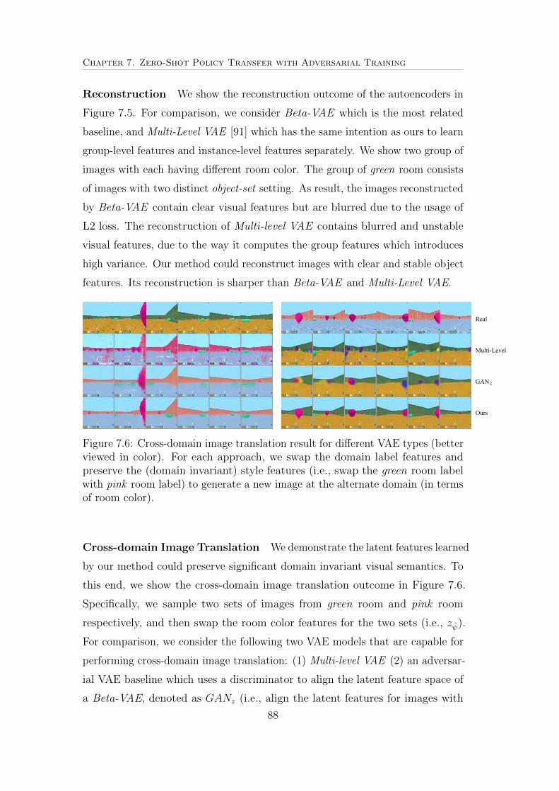
Chapter 7. Zero-Shot Policy Transfer with Adversarial Training
Reconstruction We show the reconstruction outcome of the autoencoders in
Figure 7.5. For comparison, we consider Beta-VAE which is the most related
baseline, and Multi-Level VAE [91] which has the same intention as ours to learn
group-level features and instance-level features separately. We show two group of
images with each having di↵erent room color. The group of green room consists
of images with two distinct object-set setting. As result, the images reconstructed
by Beta-VAE contain clear visual features but are blurred due to the usage of
L2 loss. The reconstruction of Multi-level VAE contains blurred and unstable
visual features, due to the way it computes the group features which introduces
high variance. Our method could reconstruct images with clear and stable object
features. Its reconstruction is sharper than Beta-VAE and Multi-Level VAE.
Real
Multi-Level
GANz
Ours
Figure 7.6: Cross-domain image translation result for di↵erent VAE types (betterviewed in color). For each approach, we swap the domain label features andpreserve the (domain invariant) style features (i.e., swap the green room labelwith pink room label) to generate a new image at the alternate domain (in termsof room color).
Cross-domain Image Translation We demonstrate the latent features learned
by our method could preserve significant domain invariant visual semantics. To
this end, we show the cross-domain image translation outcome in Figure 7.6.
Specifically, we sample two sets of images from green room and pink room
respectively, and then swap the room color features for the two sets (i.e., z ).
For comparison, we consider the following two VAE models that are capable for
performing cross-domain image translation: (1) Multi-level VAE (2) an adversar-
ial VAE baseline which uses a discriminator to align the latent feature space of
a Beta-VAE, denoted as GANz (i.e., align the latent features for images with
88

Chapter 7. Zero-Shot Policy Transfer with Adversarial Training
domain invariant labels of balloons/cake across the green room and pink room)
(note that Beta-VAE is not capable for translation, so we do not show). From
the results shown in Figure 7.6, we observe that swapping with Multi-level VAE
results in unclear domain features. Swapping with GANz could preserve clear
room color feature, but loses a significant amount of visual semantics, e.g., the
model tries to interpret a balloon as a can or a hat. Hence we conclude aligning
the latent space of VAE with simple adversarial objective as such could not
su�ce for deriving domain invariant features and we need a more sophisticated
way to align the latent space. Our approach demonstrates significantly better
cross-domain image translation performance compared to the baselines.
Target-domain Image Translation If the target domain data could preserve
significant visual semantics when translated to the source domain, we could
expect the policy trained from source domain to be more likely to work on the
target domain, i.e., we expect hat to be recognized as hat instead of balloon or
other type of objects. We show the cross-domain image translation result on
target domain data in Figure 7.7 (note that we only do this for evaluation, and
no target domain data is used for feature/policy learning). Without any access
to target domain data, such zero-shot translation is extremely challenging. When
translated from pink to green room, our model could preserve significant amount
of visual semantics, whereas in the baseline approaches, the model can hardly
recognize the object or it even mistakes object location.
89

Chapter 7. Zero-Shot Policy Transfer with Adversarial Training
Real
Multi-Level
GANz
Ours
Figure 7.7: Cross-domain image translation result using target domain data, toshow whether significant features could be preserved after the translation.
7.4.3 Zero-Shot Policy Transfer Performance in Multi-Stage Deep RL
We show the performance scores evaluated at the target domain for DeepMind
Lab task in Table 7.1. We compare DI-VAE with end-to-end methods (DQN [14]
and LSTM-A3C [27]), multi-stage RL baselines, as well as three adapted baselines
from our method which exclude one of the loss terms, LGANz
, LGANx
and Ld at
a time, denoted as DI-VAE advz
, DI-VAE advx
, and DI-VAE d respectively. Also,
we create another adversarial baseline that simply aligns feature with same label
of f�, denoted as GAN z.
1v1 3v1
DQN A3C DQN A3C
End-to-end 1.28 (± 1.17) 3.86 (± 2.24) 2.66 (± 1.97) 4.20 (± 2.00)
Beta-VAE -0.74 (± 2.31) 5.60 (± 1.77) 7.34 (± 2.25) 5.26 (± 1.87)DARLA 2.72 (± 2.15) 1.08 (± 1.02) 6.34 (± 3.18) -1.14 (± 1.88)
GANz -1.48 (± 1.73) -1.68 (± 1.67) -3.00 (± 3.09) -1.70 (± 2.10)DI-VAEadv
z
0.14 (± 1.66) 3.84 (± 1.64) 1.58 (± 2.35) 4.42 (± 1.36)DI-VAEadv
x
1.28 (± 1.90) 6.44 (± 2.90) -3.52 (± 1.98) -1.94 (± 1.45)DI-VAEd 1.62 (± 1.79) 1.82 (± 1.86) 0.12 (± 1.51) 0.44 (± 1.43)
DI-VAE 7.28 (± 1.89) 7.40 (± 2.01) 6.66 (± 2.39) 7.62 (± 1.18)
Table 7.1: Zero-shot policy transfer score evaluated at the target domain forDeepMind Lab task.
90

Chapter 7. Zero-Shot Policy Transfer with Adversarial Training
From the result shown in Table 7.1, Beta-VAE does not perform well on
1v1 setting with DQN algorithm, and DARLA does not perform well on 3v1
with LSTM-A3C. However, our model shows robust performance across the
1v1 and 3v1 settings when trained with di↵erent RL algorithms. Also, the
negative scores of GAN z show that roughly aligning the latent space would
even bring negative e↵ect for policy generalization, so that a more sophisticated
way to align the latent space is desired. Neither of DI-VAE advz
, DI-VAE advx
or
DI-VAE d outperforms our proposed method. Hence it further validates that the
combination of those three modules is necessary.
We show the performance scores evaluated at the target domain for ViZDoom
in Table 7.2. Note that the ViZDoom domain consists of a much challenging
input distribution shift compared to DeepMind Lab, and the size of object seen
by the agent is also much smaller. Overall, DI-VAE outperforms all the baseline
methods with significant margin in terms of episode reward. Hence it shows
that learning domain invariant features could significantly help the learning of
generalizable policy even in domains with challenging visual inputs like ViZDoom.
(1v1) LSTM-A3C
End-to-end 6.12 (± 4.87)DARLA 8.64 (± 5.31)Beta-VAE 14.68 (± 6.27)
GANz 7.64 (± 5.75)DI-VAEadv
z
11.3 (± 7.26)DI-VAEadv
s
6.54 (± 5.96)DI-VAEd 7.64 (± 5.76)
DI-VAE 20.52 (± 6.98)
Table 7.2: Zero-shot policy transfer score evaluated at the target domain forViZDoom.
91

Chapter 8
Conclusion and Discussion
8.1 Conclusion
In this dissertation, I introduce a study that focuses on deep RL problems from
the exploration and transfer learning perspectives.
For exploration, the study consider the problems of improving the sample
e�ciency of the exploration algorithms for deep RL via planning and curiosity-
driven reward shaping. Specifically, a planning-based exploration algorithm is
introduced which performs deep hashing to e↵ectively evaluate novelty over
future transitions. Also, a sequence-level exploration algorithm is proposed with
a novelty model that could e�ciently deal with partially observable domains
with sparse reward condition. Furthermore, considering the long training time
and the inferior performance of the current deep RL algorithms when applied to
infamously challenging task domains, a distributed deep Q-learning framework
which incorporates an exploration incentivizing mechanism is proposed to help
the model derive more meaningful experiences to update its parameters.
To study the transfer learning problems for deep RL, I introduce two algo-
rithms to tackle the policy distillation task and zero-shot policy transfer task,
respectively. The presented policy distillation algorithm could e�ciently decrease
the training time for multi-task policy model while significantly reducing the
negative transfer e↵ect. The presented zero-shot policy transfer algorithm adopts
a novel adversarial training mechanism to derive domain invariant features, with
which the policies trained on the features could generalize to unseen target
domains better.
92

Chapter 8. Conclusion and Discussion
The presented algorithms have been intensively evaluated across di↵erent
video game playing domains, including ViZDoom, Atari 2600 games, and Deep-
Mind Lab. Specifically, our proposed exploration algorithms could brought
significant performance improvement for various infamously challenging Atari
2600 games.
8.2 Discussion
Though the advancement of recent deep RL research has greatly increased the
capability of deep RL models to solve complex problems, there are still many
open questions and challenges remained. One important issue is that most
of the well studied tasks all convey limited stochasticity in their transition.
Thus, they could be relatively easily solved without much requirement over
the generalization ability of the policy. Therefore, defining a more stochastic
and realistic tasks is crucial to advance the deep RL research towards deriving
truly useful policy models that could benefit real life applications. Meanwhile,
when solving the complex problems, the model still relies on a great amount of
human experience, such as the choice of hyperparameters and model architectures.
Another promising direction for the future research is towards developing more
automated and intelligent deep RL agent that could rely less on human experience.
93

References
[1] R. S. Sutton and A. G. Barto, Reinforcement learning: An introduction,
vol. 1. MIT press Cambridge, 1998.
[2] S. Schaal and C. G. Atkeson, “Learning control in robotics,” IEEE Robotics
& Automation Magazine, vol. 17, no. 2, pp. 20–29, 2010.
[3] J. Kober, J. A. Bagnell, and J. Peters, “Reinforcement learning in robotics:
A survey,” The International Journal of Robotics Research, vol. 32, no. 11,
pp. 1238–1274, 2013.
[4] J. A. Bagnell and J. G. Schneider, “Autonomous helicopter control using
reinforcement learning policy search methods,” in Proceedings 2001 ICRA.
IEEE International Conference on Robotics and Automation (Cat. No.
01CH37164), vol. 2, pp. 1615–1620, IEEE, 2001.
[5] S. Shalev-Shwartz, S. Shammah, and A. Shashua, “Safe, multi-
agent, reinforcement learning for autonomous driving,” arXiv preprint
arXiv:1610.03295, 2016.
[6] A. E. Sallab, M. Abdou, E. Perot, and S. Yogamani, “Deep reinforcement
learning framework for autonomous driving,” Electronic Imaging, vol. 2017,
no. 19, pp. 70–76, 2017.
[7] X. Liang, L. Lee, and E. P. Xing, “Deep variation-structured reinforcement
learning for visual relationship and attribute detection,” in Proceedings of the
IEEE conference on computer vision and pattern recognition, pp. 848–857,
2017.
[8] J. C. Caicedo and S. Lazebnik, “Active object localization with deep rein-
forcement learning,” in Proceedings of the IEEE International Conference
on Computer Vision, pp. 2488–2496, 2015.
94

REFERENCES
[9] S. Mathe, A. Pirinen, and C. Sminchisescu, “Reinforcement learning for
visual object detection,” in Proceedings of the IEEE Conference on Computer
Vision and Pattern Recognition, pp. 2894–2902, 2016.
[10] A. Graves, A.-r. Mohamed, and G. Hinton, “Speech recognition with deep
recurrent neural networks,” in 2013 IEEE international conference on acous-
tics, speech and signal processing, pp. 6645–6649, IEEE, 2013.
[11] G. Hinton, L. Deng, D. Yu, G. Dahl, A.-r. Mohamed, N. Jaitly, A. Senior,
V. Vanhoucke, P. Nguyen, B. Kingsbury, et al., “Deep neural networks for
acoustic modeling in speech recognition,” IEEE Signal processing magazine,
vol. 29, 2012.
[12] R. Collobert and J. Weston, “A unified architecture for natural language
processing: Deep neural networks with multitask learning,” in Proceedings
of the 25th international conference on Machine learning, pp. 160–167, ACM,
2008.
[13] N. Kalchbrenner and P. Blunsom, “Recurrent continuous translation models,”
in Proceedings of the 2013 Conference on Empirical Methods in Natural
Language Processing, pp. 1700–1709, 2013.
[14] V. Mnih, K. Kavukcuoglu, D. Silver, A. a Rusu, J. Veness, M. G. Bellemare,
A. Graves, M. Riedmiller, A. K. Fidjeland, G. Ostrovski, S. Petersen,
A. S. C. Beattie, I. Antonoglou, D. K. H. King, D. Wierstra, S. Legg, and
D. Hassabis, “Human-level control through deep reinforcement learning,”
Nature, 2015.
[15] G. Dulac-Arnold, R. Evans, H. van Hasselt, P. Sunehag, T. Lillicrap, J. Hunt,
T. Mann, T. Weber, T. Degris, and B. Coppin, “Deep reinforcement learning
in large discrete action spaces,” arXiv preprint arXiv:1512.07679, 2015.
[16] X. Zhao, L. Xia, L. Zhang, Z. Ding, D. Yin, and J. Tang, “Deep reinforcement
learning for page-wise recommendations,” in Proceedings of the 12th ACM
Conference on Recommender Systems, pp. 95–103, ACM, 2018.
95

REFERENCES
[17] X. Zhao, L. Zhang, Z. Ding, L. Xia, J. Tang, and D. Yin, “Recommendations
with negative feedback via pairwise deep reinforcement learning,” in Pro-
ceedings of the 24th ACM SIGKDD International Conference on Knowledge
Discovery & Data Mining, pp. 1040–1048, ACM, 2018.
[18] C. Finn, P. Abbeel, and S. Levine, “Model-agnostic meta-learning for fast
adaptation of deep networks,” in Proceedings of the 34th International
Conference on Machine Learning-Volume 70, pp. 1126–1135, JMLR. org,
2017.
[19] D. Zhao, Y. Chen, and L. Lv, “Deep reinforcement learning with visual
attention for vehicle classification,” IEEE Transactions on Cognitive and
Developmental Systems, vol. 9, no. 4, pp. 356–367, 2016.
[20] Z. Ren, X. Wang, N. Zhang, X. Lv, and L.-J. Li, “Deep reinforcement
learning-based image captioning with embedding reward,” in Proceedings of
the IEEE Conference on Computer Vision and Pattern Recognition, pp. 290–
298, 2017.
[21] J. Li, W. Monroe, A. Ritter, M. Galley, J. Gao, and D. Jurafsky,
“Deep reinforcement learning for dialogue generation,” arXiv preprint
arXiv:1606.01541, 2016.
[22] I. V. Serban, C. Sankar, M. Germain, S. Zhang, Z. Lin, S. Subramanian,
T. Kim, M. Pieper, S. Chandar, N. R. Ke, et al., “A deep reinforcement
learning chatbot,” arXiv preprint arXiv:1709.02349, 2017.
[23] H. Van Hasselt, A. Guez, and D. Silver, “Deep reinforcement learning with
double q-learning,” in AAAI, pp. 2094–2100, 2016.
[24] M. Hessel, J. Modayil, H. Van Hasselt, T. Schaul, G. Ostrovski, W. Dabney,
D. Horgan, B. Piot, M. Azar, and D. Silver, “Rainbow: Combining improve-
ments in deep reinforcement learning,” in Thirty-Second AAAI Conference
on Artificial Intelligence, 2018.
[25] D. Silver, A. Huang, C. J. Maddison, A. Guez, L. Sifre, G. Van Den Driessche,
J. Schrittwieser, I. Antonoglou, V. Panneershelvam, M. Lanctot, et al.,
“Mastering the game of go with deep neural networks and tree search,”
nature, vol. 529, no. 7587, p. 484, 2016.
96

REFERENCES
[26] M. Fortunato, M. G. Azar, B. Piot, J. Menick, I. Osband, A. Graves,
V. Mnih, R. Munos, D. Hassabis, O. Pietquin, et al., “Noisy networks for
exploration,” arXiv preprint arXiv:1706.10295, 2017.
[27] V. Mnih, A. P. Badia, M. Mirza, A. Graves, T. P. Lillicrap, T. Harley, D. Sil-
ver, and K. Kavukcuoglu, “Asynchronous methods for deep reinforcement
learning,” in International Conference on Machine Learning, 2016.
[28] Z. Wang, T. Schaul, M. Hessel, H. van Hasselt, M. Lanctot, and N. de Freitas,
“Dueling network architectures for deep reinforcement learning,” in ICML,
pp. 1995–2003, 2016.
[29] M. G. Bellemare, W. Dabney, and R. Munos, “A distributional perspective
on reinforcement learning,” arXiv preprint arXiv:1707.06887, 2017.
[30] B. F. Skinner, The behavior of organisms: An experimental analysis. BF
Skinner Foundation, 1990.
[31] S. P. Singh, “Transfer of learning by composing solutions of elemental
sequential tasks,” Machine Learning, vol. 8, no. 3-4, pp. 323–339, 1992.
[32] M. Dorigo and M. Colombetti, “Robot shaping: Developing autonomous
agents through learning,” Artificial intelligence, vol. 71, no. 2, pp. 321–370,
1994.
[33] A. Y. Ng, D. Harada, and S. Russell, “Policy invariance under reward
transformations: Theory and application to reward shaping,” in ICML,
vol. 99, pp. 278–287, 1999.
[34] M. Grzes and D. Kudenko, “Reward shaping and mixed resolution function
approximation,” Developments in Intelligent Agent Technologies and Multi-
Agent Systems: Concepts and Applications, p. 95, 2010.
[35] N. Chentanez, A. G. Barto, and S. P. Singh, “Intrinsically motivated rein-
forcement learning,” in Advances in neural information processing systems,
pp. 1281–1288, 2005.
97

REFERENCES
[36] H. Tang, R. Houthooft, D. Foote, A. Stooke, X. Chen, Y. Duan, J. Schulman,
F. De Turck, and P. Abbeel, “# exploration: A study of count-based explo-
ration for deep reinforcement learning,” arXiv preprint arXiv:1611.04717,
2016.
[37] G. Ostrovski, M. G. Bellemare, A. v. d. Oord, and R. Munos, “Count-based
exploration with neural density models,” in International Conference on
Machine Learning, 2017.
[38] D. Pathak, P. Agrawal, A. A. Efros, and T. Darrell, “Curiosity-driven
exploration by self-supervised prediction,” in International Conference on
Machine Learning (ICML), vol. 2017, 2017.
[39] X. Guo, S. Singh, H. Lee, R. L. Lewis, and X. Wang, “Deep learning for
real-time atari game play using o✏ine monte-carlo tree search planning,” in
Advances in neural information processing systems, pp. 3338–3346, 2014.
[40] L. Kocsis and C. Szepesvari, “Bandit based monte-carlo planning,” in
European conference on machine learning, pp. 282–293, Springer, 2006.
[41] J. Oh, X. Guo, H. Lee, R. L. Lewis, and S. Singh, “Action-conditional
video prediction using deep networks in atari games,” in Advances in Neural
Information Processing Systems 28, pp. 2845–2853, Curran Associates, Inc.,
2015.
[42] R. Pascanu, Y. Li, O. Vinyals, N. Heess, L. Buesing, S. Racaniere, D. Re-
ichert, T. Weber, D. Wierstra, and P. Battaglia, “Learning model-based
planning from scratch,” arXiv preprint arXiv:1707.06170, 2017.
[43] T. Weber, S. Racaniere, D. P. Reichert, L. Buesing, A. Guez, D. J. Rezende,
A. P. Badia, O. Vinyals, N. Heess, Y. Li, et al., “Imagination-augmented
agents for deep reinforcement learning,” arXiv preprint arXiv:1707.06203,
2017.
[44] M. Bellemare, S. Srinivasan, G. Ostrovski, T. Schaul, D. Saxton, and
R. Munos, “Unifying count-based exploration and intrinsic motivation,” in
NIPS, pp. 1471–1479, 2016.
98
REFERENCES
[45] L. Espeholt, H. Soyer, R. Munos, K. Simonyan, V. Mnih, T. Ward, Y. Doron,
V. Firoiu, T. Harley, I. Dunning, et al., “Impala: Scalable distributed deep-
rl with importance weighted actor-learner architectures,” arXiv preprint
arXiv:1802.01561, 2018.
[46] D. Horgan, J. Quan, D. Budden, G. Barth-Maron, M. Hessel, H. Van Hasselt,
and D. Silver, “Distributed prioritized experience replay,” arXiv preprint
arXiv:1803.00933, 2018.
[47] S. Kapturowski, G. Ostrovski, J. Quan, R. Munos, and W. Dabney, “Recur-
rent experience replay in distributed reinforcement learning,” 2018.
[48] C. Bucilu, R. Caruana, and A. Niculescu-Mizil, “Model compression,” in
SIGKDD, pp. 535–541, ACM, 2006.
[49] G. Hinton, O. Vinyals, and J. Dean, “Distilling the knowledge in a neural
network,” in NIPS Workshop on Deep Learning and Representation Learning,
2014.
[50] Z. Tang, D. Wang, Y. Pan, and Z. Zhang, “Knowledge transfer pre-training,”
arXiv preprint arXiv:1506.02256, 2015.
[51] J. Li, R. Zhao, J.-T. Huang, and Y. Gong, “Learning small-size dnn with
output-distribution-based criteria.,” in Interspeech, pp. 1910–1914, 2014.
[52] A. Romero, N. Ballas, S. E. Kahou, A. Chassang, C. Gatta, and Y. Bengio,
“Fitnets: Hints for thin deep nets,” in ICLR, 2015.
[53] A. A. Rusu, S. G. Colmenarejo, C. Gulcehre, G. Desjardins, J. Kirkpatrick,
R. Pascanu, V. Mnih, K. Kavukcuoglu, and R. Hadsell, “Policy distillation,”
in ICLR, 2016.
[54] E. Parisotto, J. Ba, and R. Salakhutdinov, “Actor-mimic deep multitask
and transfer reinforcement learning,” in ICLR, 2016.
[55] A. Gupta, C. Devin, Y. Liu, P. Abbeel, and S. Levine, “Learning invariant fea-
ture spaces to transfer skills with reinforcement learning,” arXiv:1703.02949,
2017.
99

REFERENCES
[56] E. Tzeng, C. Devin, J. Ho↵man, C. Finn, P. Abbeel, S. Levine, K. Saenko,
and T. Darrell, “Adapting deep visuomotor representations with weak
pairwise constraints,” arXiv:1511.07111, 2015.
[57] E. Tzeng, J. Ho↵man, K. Saenko, and T. Darrell, “Adversarial discriminative
domain adaptation,” in Computer Vision and Pattern Recognition (CVPR),
vol. 1, p. 4, 2017.
[58] S. Daftry, J. A. Bagnell, and M. Hebert, “Learning transferable policies for
monocular reactive mav control,” in International Symposium on Experi-
mental Robotics, pp. 3–11, 2016.
[59] B. Da Silva, G. Konidaris, and A. Barto, “Learning parameterized skills,”
arXiv:1206.6398, 2012.
[60] D. Isele, M. Rostami, and E. Eaton, “Using task features for zero-shot
knowledge transfer in lifelong learning.,” in IJCAI, pp. 1620–1626, 2016.
[61] T. Schaul, D. Horgan, K. Gregor, and D. Silver, “Universal value function
approximators,” in ICML, 2015.
[62] J. Oh, S. Singh, H. Lee, and P. Kohli, “Zero-shot task generalization with
multi-task deep reinforcement learning,” ICML, 2017.
[63] I. Higgins, A. Pal, A. A. Rusu, L. Matthey, C. P. Burgess, A. Pritzel,
M. Botvinick, C. Blundell, and A. Lerchner, “Darla: Improving zero-shot
transfer in reinforcement learning,” 2017.
[64] I. Higgins, L. Matthey, A. Pal, C. Burgess, X. Glorot, M. Botvinick, S. Mo-
hamed, and A. Lerchner, “beta-vae: Learning basic visual concepts with a
constrained variational framework,” in ICLR, 2016.
[65] H. Yin, J. Chen, and S. J. Pan, “Hashing over predicted future frames for
informed exploration of deep reinforcement learning,” 2018.
[66] D. P. Kingma and M. Welling, “Auto-encoding variational bayes,” in ICLR,
2014.
100

REFERENCES
[67] M. S. Charikar, “Similarity estimation techniques from rounding algorithms,”
in Proceedings of the thiry-fourth annual ACM symposium on Theory of
computing, pp. 380–388, ACM, 2002.
[68] M. G. Bellemare, Y. Naddaf, J. Veness, and M. Bowling, “The arcade
learning environment: An evaluation platform for general agents,” Journal
of Artificial Intelligence Research, vol. 47, pp. 253–279, Jun 2013.
[69] D. P. Kingma and J. Ba, “Adam: A method for stochastic optimization.,”
CoRR, vol. abs/1412.6980, 2014.
[70] T. Schaul, J. Quan, I. Antonoglou, and D. Silver, “Prioritized experience
replay,” in ICLR, 2016.
[71] S. B. Thrun, “E�cient exploration in reinforcement learning,” 1992.
[72] Y. Burda, H. Edwards, A. Storkey, and O. Klimov, “Exploration by random
network distillation,” arXiv preprint arXiv:1810.12894, 2018.
[73] J. Achiam and S. Sastry, “Surprise-based intrinsic motivation for deep
reinforcement learning,” 2017.
[74] T. Pohlen, B. Piot, T. Hester, M. G. Azar, D. Horgan, D. Budden,
G. Barth-Maron, H. van Hasselt, J. Quan, M. Vecerık, et al., “Observe and
look further: Achieving consistent performance on atari,” arXiv preprint
arXiv:1805.11593, 2018.
[75] J. Schulman, F. Wolski, P. Dhariwal, A. Radford, and O. Klimov, “Proximal
policy optimization algorithms,” arXiv preprint arXiv:1707.06347, 2017.
[76] N. Savinov, A. Raichuk, D. Vincent, R. Marinier, M. Pollefeys, T. Lillicrap,
and S. Gelly, “Episodic curiosity through reachability,” in ICLR, 2019.
[77] I. Sorokin, A. Seleznev, M. Pavlov, A. Fedorov, and A. Ignateva, “Deep
attention recurrent q-network,” arXiv preprint arXiv:1512.01693, 2015.
[78] P. Mirowski, R. Pascanu, F. Viola, H. Soyer, A. J. Ballard, A. Banino,
M. Denil, R. Goroshin, L. Sifre, K. Kavukcuoglu, et al., “Learning to
navigate in complex environments,” arXiv preprint arXiv:1611.03673, 2016.
101

REFERENCES
[79] I. Sutskever, J. Martens, and G. E. Hinton, “Generating text with recurrent
neural networks,” in ICML, pp. 1017–1024, 2011.
[80] I. Osband, J. Aslanides, and A. Cassirer, “Randomized prior functions for
deep reinforcement learning,” in NeurIPS, pp. 8617–8629, 2018.
[81] M. Kempka, M. Wydmuch, G. Runc, J. Toczek, and W. Jaskowski, “ViZ-
Doom: A Doom-based AI research platform for visual reinforcement learning,”
in CIG, pp. 341–348, 2016.
[82] C. Beattie, J. Z. Leibo, D. Teplyashin, T. Ward, M. Wainwright, H. Kuttler,
A. Lefrancq, S. Green, V. Valdes, A. Sadik, et al., “Deepmind lab,”
arXiv:1612.03801, 2016.
[83] H. Yin and S. J. Pan, “Knowledge transfer for deep reinforcement learning
with hierarchical experience replay,” in Thirty-First AAAI Conference on
Artificial Intelligence, 2017.
[84] S. J. Pan and Q. Yang, “A survey on transfer learning,” IEEE Transactions
on Knowledge and Data Engineering, vol. 22, no. 10, pp. 1345–1359, 2010.
[85] M. T. Rosenstein, Z. Marx, L. P. Kaelbling, and T. G. Dietterich, “To
transfer or not to transfer,” in NIPS Workshop on Inductive Transfer: 10
Years Later, 2005.
[86] L.-J. Lin, Reinforcement Learning for Robots Using Neural Networks. PhD
thesis, Pittsburgh, PA, USA, 1992. UMI Order No. GAX93-22750.
[87] T. Tieleman and G. Hinton, “Lecture 6.5-rmsprop: Divide the gradient by
a running average of its recent magnitude,” COURSERA: Neural Networks
for Machine Learning, 2012.
[88] Y. Bengio, A. Courville, and P. Vincent, “Representation learning: A review
and new perspectives,” IEEE transactions on pattern analysis and machine
intelligence, vol. 35, no. 8, pp. 1798–1828, 2013.
[89] J. Harrison, A. Garg, B. Ivanovic, Y. Zhu, S. Savarese, L. Fei-Fei, and
M. Pavone, “Adapt: zero-shot adaptive policy transfer for stochastic dy-
namical systems,” arXiv:1707.04674, 2017.
102

REFERENCES
[90] C. Finn, X. Y. Tan, Y. Duan, T. Darrell, S. Levine, and P. Abbeel, “Deep
spatial autoencoders for visuomotor learning,” in 2016 IEEE International
Conference on Robotics and Automation (ICRA), pp. 512–519, 2016.
[91] D. Bouchacourt, R. Tomioka, and S. Nowozin, “Multi-level variational
autoencoder: Learning disentangled representations from grouped observa-
tions,” arXiv:1705.08841, 2017.
103