IMPROVING DATA QUALITY CONTROL IN THE XPLAIN-DBMS

IMPROVING DATA QUALITY CONTROL IN THE XPLAIN-DBMS J.A. Bakker

Retired assistant professor of database systems,

Faculty of Electrical Engineering, Mathematics and Computer Systems,

Delft University of Technology, the Netherlands

Email: [email protected]

ABSTRACT

This paper discusses the usability of convertibility, a principle for data quality used by the Xplain-DBMS.

Convertibility (uniqueness) of type definitions is a helpful criterion for database design, whereas convertibility of

instances is a criterion for the uniqueness of instances (records). However, in many situations with or without

generalization/specialization, convertibility appears to be an insufficient criterion for correctness of instances,

which is illustrated by many examples. In order to be able to specify more rigorous rules for correctness of

instances we propose to use new concepts such as ‘identifying property’. These new concepts also facilitate the

transformation of relational databases into Xplain databases.

Keywords: Convertibility, Entity correctness, Generalization, Specialization, Transaction, Xplain-DBMS

1 INTRODUCTION

Data Base Management Systems (DBMS) offer sharing of integrated data (reducing data redundancy) and

maintenance of entity integrity (correctness) and referential integrity on the basis of a conceptual data model and

restrictions complying with organizational structure and information needs (Elmasri & Navathe, 2010; Connolly,

Begg, & Strachan, 1995). Databases are the core of many information systems and can contain enormous data

collections (terabytes to petabytes) that are vital for many large organizations, such as the U.S. federal government,

insurance companies, NASA, UPS, etc.

An essential part of a database is a conceptual data model that defines its logical data structure. For example, in a

relational DBMS a project database of some organization can be based on the following data model, specified in

terms of relations and attributes (an informal specification without value domains):

relation project (proj#, description, starting_date, final_date);

relation employee (emp#, name, address, town, birth_date, salary);

relation work (work#, emp#, proj#, date, worked_hours);

relation invoice (inv#, description, date, amount).

Here an underlined attribute is a primary key (its value must be unique), whereas foreign keys are presented in italic

type face (their value must exist among the primary key values of the referenced relation). Foreign keys are essential

for maintaining referential integrity, which means here that records of the relation “work” must contain foreign key

values already existing in a record (tuple) of “employee” (emp#) and a record of “project” (proj#). Moreover,

records may not be removed from the database as long as they are referenced by other records. Using the relational

language SQL we can define such a model including explicit constraints for primary and foreign keys.

An option is to apply a “NOT NULL” statement, which is mandatory for primary keys, but not for other attributes,

including foreign key attributes. In the last case the interpretation of “null” probably is “unknown” or “irrelevant”.

However, a foreign key having a “null” value is violating referential integrity. Maintaining referential integrity is

essential for calculating derivable data such as the sum of worked hours for each project, therefore it makes sense to

add a “NOT NULL” rule to the definition of a foreign key such as “work.proj#”.

Ad hoc data manipulation by experts is supported by a query language (SQL in relational systems). An example is

the following query deriving the total of worked hours in projects per employee:

Data Science Journal, Volume 11, 10 March 2012

1

mailto:[email protected]

SELECT employee.emp#, SUM(worked_hours)

FROM work, employee

WHERE work.emp# = employee.emp# /* an equi-join

GROUP BY employee.emp#

UNION

SELECT employee.emp#, 0 /* sum of worked hours = 0

FROM employee

WHERE employee.emp# NOT IN (SELECT emp# FROM work).

This query illustrates that the semantics of SQL, especially the GROUP BY construct, is not simply understandable.

The first selection using an equi-join only selects the employees who worked for any project. The second selection

(after “UNION”) produces data on employees who did not work for any project at all. In other words, the first sub-

query without the union produces only a correct result if all employees worked for any project. This first sub query

alone is incorrect (incomplete) because a query has to produce correct and complete results irrespective the database

contents.

Another source of problems is that SQL allows joining tables that do not have any structural relationship (through a

matching pair of a primary and a foreign key). In order to demonstrate this pitfall, the relation “invoice” is part of

the example model, which enables us to specify the following query:

SELECT work.proj#, work.date, invoice.amount

FROM work, invoice

WHERE work.date = invoice.date;

The last query ignores the structure of the data model and can produce a result table where the same amount is

coupled to many projects: the well known connection trap (Codd, 1970). In order to avoid such semantic problems

it is advisable that naive users use standard applications. For further discussions on (dis)advantages of DBMS’s we

refer to text books (Rolland, 1998; Elmasri & Navathe, 2010; Connolly, Begg, & Strachan, 1995).

Data security in a local database management system can be managed on the basis of user privileges registered in an

authorization scheme. However, when a database is accessible via the Internet, other security problems can arise

often caused by improperly specified queries (North, 2010). For example, SQL allows joining relations (tables) even

without any join condition: a Cartesian product, possibly requiring a very long execution time. This product of two

tables contains N *M results if there are N records in a table and M records in the other table. One might wonder

whether it makes sense that SQL enables users to generate more data than present in the underlying database.

In order to prevent these problems related to SQL, a first objective of Johan ter Bekke was to design a data language

without these problems. Soon he discovered that this also required designing new concepts for data modeling.

Inspired by publications of Smith and Smith (1977) on aggregation and generalization as construction principles for

data models he developed new concepts for data modeling and data manipulation (ter Bekke, 1980, 1991, 1992). In

order to enhance data quality control in the Xplain-DBMS Johan ter Bekke also developed well separated categories

of restrictions for data models: inherent and explicit restrictions.

Inherent restrictions (convertibility and referential integrity, Section 1.2) are a logical consequence of a data model.

Convertibility means that a type is identified not only by a name, but also by a set of attributes, and reversely, a set

of attributes identifies a type. At the implementation level convertibility is a criterion for the uniqueness of

instances: instances belonging to the same object type must have a single identifier and a unique collection of

attribute values.

Explicit restrictions - such as business rules - are not inherent in an Xplain data model. We can distinguish static

restrictions (Section 1.3) and dynamic restrictions (Section 1.4). Section 1.3 also discusses the meta model of Xplain

for the data dictionary. Section 1.5 introduces the concept of generalization/specialization, whereas Section 1.6

shows the strict relationship between data structure and data manipulation (also for recursive operations) in Xplain.

The next Section gives a motivation for writing the present paper.


2

1.1 Motivation

Johan ter Bekke briefly wrote in his first Dutch textbook (ter Bekke, 1983) that convertibility is required over the

combination of generalization and specialization. In his later textbooks such a remark can no longer be found.

Probably he was aware of some unsolved problems and still working on a solution when he suddenly passed away in

March 2004.

It is the objective of the present paper to identify these problems and to propose a generic solution for diverse

situations with or without generalization/specialization in data models. The present paper will clarify that there are

two problems related to convertibility of instances:

1. Convertibility is not always a satisfactory criterion for the correctness of instances, which requires the design of

new rules for correctness of instances.

2. Depending on the kind of generalization/specialization it is necessary to specify different rules for the

correctness of instances.

Before starting an extensive discussion on problems and solutions we give an overview of the principles for data

definition and manipulation of the Xplain-DBMS in Sections 1.2 - 1.6.

1.2 Inherent restrictions

Convertibility or uniqueness of type definitions

In the Xplain-DBMS each type is identified by a name and at the same time also by a set of relevant attributes (ter

Bekke, 1980). Reversely, a certain set of attributes identifies a type as well. This is the principle of convertibility of

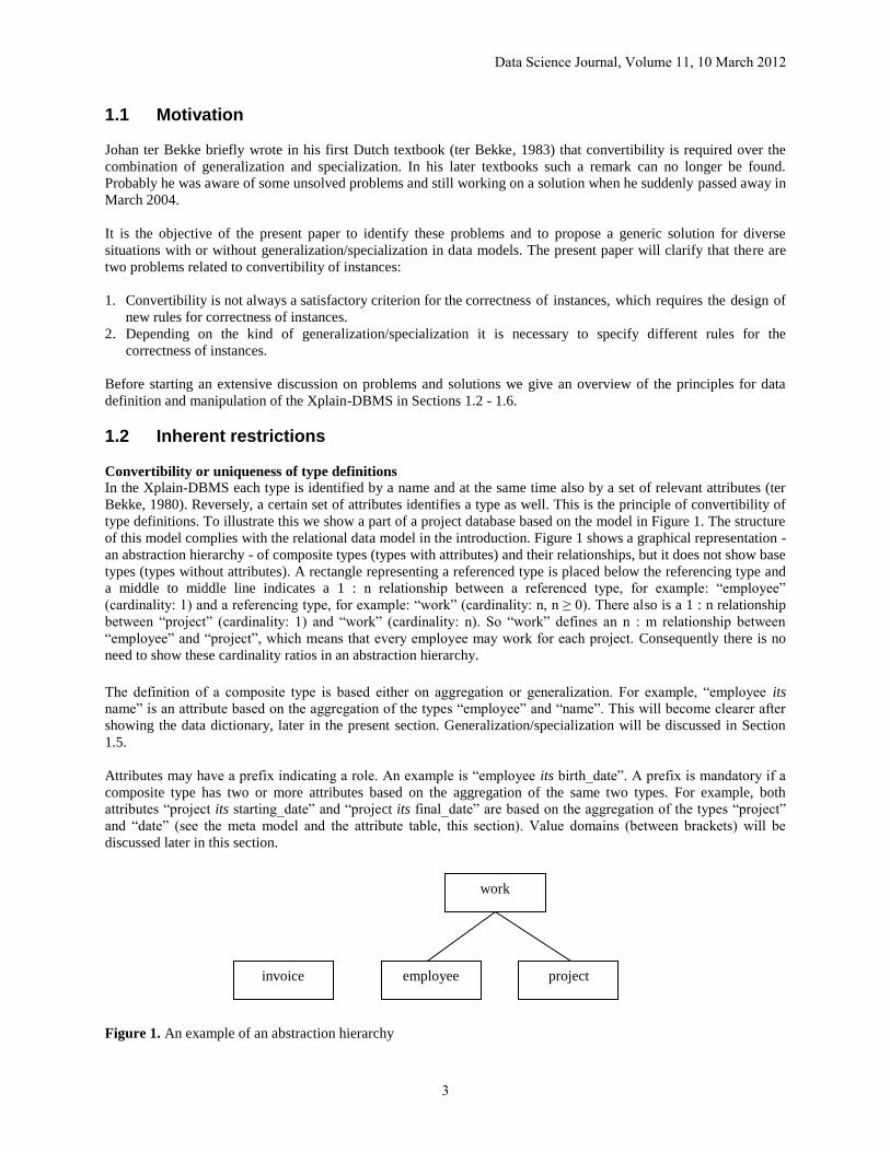
type definitions. To illustrate this we show a part of a project database based on the model in Figure 1. The structure

of this model complies with the relational data model in the introduction. Figure 1 shows a graphical representation -

an abstraction hierarchy - of composite types (types with attributes) and their relationships, but it does not show base

types (types without attributes). A rectangle representing a referenced type is placed below the referencing type and

a middle to middle line indicates a 1 : n relationship between a referenced type, for example: “employee”

(cardinality: 1) and a referencing type, for example: “work” (cardinality: n, n ≥ 0). There also is a 1 : n relationship

between “project” (cardinality: 1) and “work” (cardinality: n). So “work” defines an n : m relationship between

“employee” and “project”, which means that every employee may work for each project. Consequently there is no

need to show these cardinality ratios in an abstraction hierarchy.

The definition of a composite type is based either on aggregation or generalization. For example, “employee its

name” is an attribute based on the aggregation of the types “employee” and “name”. This will become clearer after

showing the data dictionary, later in the present section. Generalization/specialization will be discussed in Section

1.5.

Attributes may have a prefix indicating a role. An example is “employee its birth_date”. A prefix is mandatory if a

composite type has two or more attributes based on the aggregation of the same two types. For example, both

attributes “project its starting_date” and “project its final_date” are based on the aggregation of the types “project”

and “date” (see the meta model and the attribute table, this section). Value domains (between brackets) will be

discussed later in this section.

Figure 1. An example of an abstraction hierarchy

work

employee

project

invoice


3

Figure 1 is based on the following definitions:

base name (A12). base date (D). base address (A20). base town (A22).

base description (A18). base salary (R4,2). base hours (I4). base amount (R5,2).

type work (I5) = employee, project, date, worked_hours.

type project (I3) = description, starting_date, final_date.

type employee (I3) = name, address, town, birth_date, salary.

type invoice (I3) = description, date, amount.

A consequence of convertibility is that the following definitions may not be part of the previous data model:

type activity (I3) = description, starting_date, final_date. /* already defined set of attributes

type employee (I3) = first_name, last_name, address, town, birth_date, salary. /* “employee”: already defined

Based on the model in Figure 1, we can specify a query in the Xplain language deriving the total number of hours

worked in projects per employee. In Xplain nested queries and joins may not and cannot be specified, so we start

with the derivation of the total worked project hours per employee (“employee its project hours”):

extend employee with project hours = total work its worked_hours

per employee. /* “per” means: for all instances of “employee”

get employee its name, project hours. /* employee identifier is automatically included

In the last extend operation the referential path “work its employee” is used, which avoids the need of specifying any

join operation. Contrary to SQL, Xplain requires to apply a path existing in a data model. In this way the connection

trap is avoided (ter Bekke & Bakker, 2001).

Value domains and value restrictions

The following value representations (value domains) are supported by the Xplain-DBMS:

In: integer consisting of at most n decimal digits.

An: alpha-numeric string with at most n characters.

Rn,m: real with at most n decimal digits before and m decimal digits after the decimal point.

B: Boolean variable, its value is either true or false.

D: dates specified by decimal digits using the format “yyyymmdd”.

Xplain also supports value restrictions such as ranges, enumeration and patterns (not shown here). In some later

examples we will show assertions containing a value range indicating a value restriction.

Convertibility (uniqueness) of instances

Convertibility of type definitions (conceptual level) implies that convertibility is also required at the implementation

level: each instance of a composite type must have a single unmodifiable identifier (unique within that type) and at

the same time the set of all its attribute values must be unique. The set of attributes can be considered as a kind of

key. It is a modifiable key, so it is better to speak of an identifying property.

Convertibility of instances is a weak criterion for entity correctness because often uniqueness is required for only

some of the attributes. For example, a business rule could be that instances of “project” must have a unique

description. This weakness will be discussed further in Sections 2 - 5.

Relatability (referential integrity)

In the data language of Xplain a term - depending on its context - may have different interpretations. For example

“employee” indicates a composite type, but “employee” can also be considered as an attribute of the type “work”.

This example of a kind of object relativity implies an inherent reference from the type “work” to the type

“employee” via the referencing attribute “work its employee”. So there is no need to specify any explicit subset

constraint supporting referential integrity, which is a contrast to the explicit foreign key statement of SQL

(Connolly, Begg, & Strachan, 1995).


4

Meta model (model of the data dictionary)

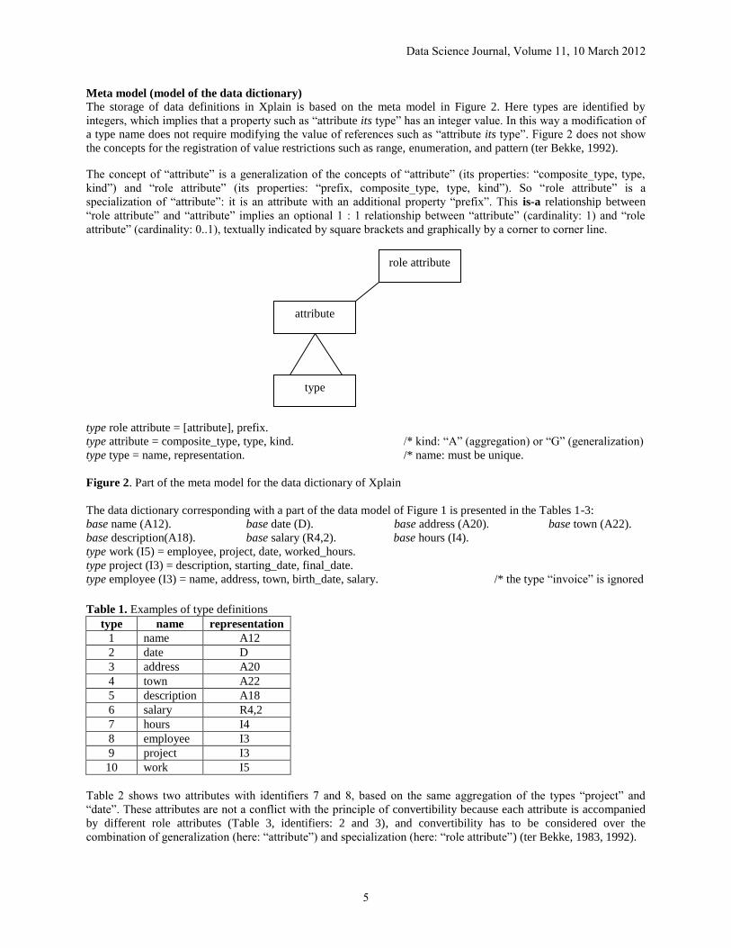
The storage of data definitions in Xplain is based on the meta model in Figure 2. Here types are identified by

integers, which implies that a property such as “attribute its type” has an integer value. In this way a modification of

a type name does not require modifying the value of references such as “attribute its type”. Figure 2 does not show

the concepts for the registration of value restrictions such as range, enumeration, and pattern (ter Bekke, 1992).

The concept of “attribute” is a generalization of the concepts of “attribute” (its properties: “composite_type, type,

kind”) and “role attribute” (its properties: “prefix, composite_type, type, kind”). So “role attribute” is a

specialization of “attribute”: it is an attribute with an additional property “prefix”. This is-a relationship between

“role attribute” and “attribute” implies an optional 1 : 1 relationship between “attribute” (cardinality: 1) and “role

attribute” (cardinality: 0..1), textually indicated by square brackets and graphically by a corner to corner line.

type role attribute = [attribute], prefix.

type attribute = composite_type, type, kind. /* kind: “A” (aggregation) or “G” (generalization)

type type = name, representation. /* name: must be unique.

Figure 2. Part of the meta model for the data dictionary of Xplain

The data dictionary corresponding with a part of the data model of Figure 1 is presented in the Tables 1-3:

base name (A12). base date (D). base address (A20). base town (A22).

base description(A18). base salary (R4,2). base hours (I4).

type work (I5) = employee, project, date, worked_hours.

type project (I3) = description, starting_date, final_date.

type employee (I3) = name, address, town, birth_date, salary. /* the type “invoice” is ignored

Table 1. Examples of type definitions

type name representation

1 name A12

2 date D

3 address A20

4 town A22

5 description A18

6 salary R4,2

7 hours I4

8 employee I3

9 project I3

10 work I5

Table 2 shows two attributes with identifiers 7 and 8, based on the same aggregation of the types “project” and

“date”. These attributes are not a conflict with the principle of convertibility because each attribute is accompanied

by different role attributes (Table 3, identifiers: 2 and 3), and convertibility has to be considered over the

combination of generalization (here: “attribute”) and specialization (here: “role attribute”) (ter Bekke, 1983, 1992).

role attribute

attribute

type


5

Table 2. Examples of attribute definitions

attribute composite_type type kind

1 8 /* employee 1 /* name A

2 8 3 /* address A

3 8 4 /* town A

4 8 2 /* date A

5 8 6 /* salary A

6 9 /* project 5 /* description A

7 9 2 /* date A

8 9 2 /* date A

9 10 /* work 8 /* employee A

10 10 9 /* project A

11 10 7 /* hours A

12 10 2 /* date A

Table 3. Examples of role attribute definitions

role attribute [attribute] prefix

1 4 /* employee its birth_date birth

2 7 /* project its starting_date starting

3 8 /* project its final_date final

4 11 /* work its worked_hours worked

1.3 Static restrictions

In Xplain static restrictions are specified in terms of derived data using assertions, which means that these rules are

based on controlled redundancy. An assertion applies to a database state at any time and cannot be specified

inherently in a data model. In many cases an assertion complies with a business rule. An example is that a project

ends at a later date than the starting date. This can be expressed by a derived attribute “project its correctness”, its

calculation and a value restriction “(true)”. If the final date is not known yet, a special value as “99991231” should

be applied (see Section 1.4).

assert project its correctness (true) = (final_date > starting_date).

Another requirement is that “work its date” complies with the project dates:

assert work its date correctness (true) = (date >= project its starting_date and date <= project its final_date).

Other examples of applying assertions are related to a model for orders and order lines (without showing value

domains). An attribute between slashes is derived by an assertion:

type order line = order, article, price, number, /amount/. /* “amount” is a derived attribute

type order = customer, date, /total amount/, /line number/. /* “total amount”, “line number”: derived attributes

assert order line its amount (0..*) = number * price. /* “price”: property of “order line”

assert order its total amount (0..*) = total order line its amount per order. /* “total”: a set function

assert order its line number (1..*) = count order line per order. /* “count”: another set function

Apparently convertibility is a weak correctness principle: it allows two or more instances of “order line” with the

same values for the attribute combination (“order, article, price”) but with different values for “number”. Such a

duplication should not be allowed. Moreover, it leads to an incorrect calculation of the derived attributes “order its

total amount” and “order its line number”. A further discussion of similar problems will be presented in Section 2.


6

1.4 Dynamic restrictions

Dynamic restrictions have to deal with the correctness of database state transitions (insertions and updates). An

example of an insert restriction is associated with the following model, a slight modification of the previous model.

Now the amount of an order line is calculated automatically at insertion time only using the init command.

Therefore later updates of “article its price” do not affect the earlier registered data on “order line its amount”.

type order line = order, article, number, amount.

type order = customer, date, /total amount/, /line number/.

type article = name, price. /* here: a price per article

assert order its total amount (0..*) = total order line its amount per order.

assert order its line number (1..*) = count order line per order.

init order line its amount = number * article its price. /* only valid at insertion time

Errors in order dates can be prevented by using a default value for order dates:

init default order its date = systemdate. /* only valid at insertion time

If a final date in the example in Section 1.2 is not known at insertion time, we might apply:

init default project its final_date = 99991231.

We do not show how update restrictions (ter Bekke, 1992) are specified. An example is that, at the end of a school

year, pupils only may move to a higher class level or leave the school or have to stay at the same level, whereas

during a school year a degradation to a lower level is possible. So there is a distinct number of updates (transitions)

allowed for the value of an attribute, such as “pupil its class_level”.

Explicit delete restrictions make no sense because a deletion is a transition from an existing state to an empty state,

whereas implicit delete restrictions are a consequence of inherent rules such as referential integrity or assertions. For

example: an order must have at least one order line, therefore a single remaining order line may not be deleted

without deleting the involved order.

1.5 Generalization/specialization

Aggregation is not the only constructing principle for data modeling; Xplain also supports generalization/

specialization. This is a useful design concept when almost similar object types, for example “office” and “house”,

have the same properties such as “address” and “construction_year”, etc, but differ in terms of other properties. The

common properties can be considered to belong to their generalization (here: “building”), whereas distinguishing

properties belong to a specialization type. The following definitions mean that a building is a house or an office and

is not both at the same time (ter Bekke, 1992). Therefore, an example of a data model for a real estate agency (figure

3) shows an example of disjoint specialization:

type office = [building], office type, floor space.

type house = [building], sort, number of rooms.

type building = address, construction_year, purchase_date, price, owner.

type sale = building, date, price, new owner.

Figure 3. A data model (abstraction hierarchy) with disjoint specialization

sale office

house

building


7

The following alternative requires applying two “null” values for each instance of “building’, which is a source of

insertion errors because this simpler model does not explain which attributes must have a “null” value in which case:

type building = address, construction_year, purchase_date, price, owner,

office type, floor space, sort, number of rooms.

This application of generalization (Figure 3) avoids this insertion problem and makes it easier to specify retrievals

addressing only the common properties of both kinds of buildings. Another advantage is that other types, such as

“sale”, may refer to the generalization (e.g. “sale its building”), which makes it easier to specify retrievals of sales

irrespective the kind of sold object. Without generalization/specialization, we would have to define two partially

overlapping building types (“house” and “office”) and two types for sale results: “house sale” and “office sale”. The

same applies to retrieving all sale results. Using generalization/specialization, each composite type can be defined in

terms of definitive properties (attributes) relevant to all instances of that type. Contrary to SQL, there is no need to

use a “null” value if an attribute is irrelevant, which is essential for deriving data and referential integrity as well. In

relational databases, “null” can also have other interpretations such as “unknown” or “zero” (ter Bekke, 1997).

1.6 Relationship between data structure and data manipulation

Xplain requires a strict relationship between data structure (data model) and data manipulation. Definitive properties

(intrinsic or inherited) are always found by using an existing path in a data model. It is not allowed and not possible

to join data. For example, the following query retrieves some properties of work data and related data inherited of

employees who worked for project 345:

type work = employee, project, date, worked_hours.

type project = description, starting_date, final_date.

type employee = name, address, town, birth_date, salary.

get work its employee, employee its name, date, worked_hours

where project = 345. /* means the same as “where work its project = 345”

In the last query we see that the attributes “work its employee” (also a reference), “work its worked_hours”, and a

longer path “work its employee its name” are specified. If an employee worked on more than one day for project

345, then this query generates many copies of the same employee data. A better query avoids this replication of

results and will be shown later.

In SQL there is not such a clear relationship between data structure (defined by a matching pair of primary and

foreign keys) and data manipulation. We refer to the example in the introduction of Section 1, where two relational

tables (“work” and “invoice”) are joined over two non-key attributes. We already showed in Section 1 that the

“GROUP BY” construct of SQL has a meaning other than the “per” construct of Xplain.

In cases where derivable data have to be retrieved, Xplain requires starting with an extend operation calculating the

desired derivable property. For example, the following query retrieves the name and salary of employees who

worked for project 345. Now the result does not contain any repetition of the same retrieved data on employees:

extend employee with involved = any work where project = 345 /* deriving “employee its involved”

per employee. /* used path: “work its employee”

get employee its name, salary

where involved. /* using “employee its involved”

Also in the case of recursive queries (for example, finding the shortest path (over arcs) between two points (nodes)

in a network (graph)) it is essential that data structure is respected. Earlier solutions for recursive problems such as

transitive closure (Aho, Hopcroft, & Ullman, 1974; Bailey, 1999; Connolly, Begg, & Strachan, 1995; Dar &

Ramakrishnan, 1994; Suciu & Paredaens, 1994; Ullman & Widom, 1997) often create successor lists much larger

than the original data set, which leads to time-consuming duplicate elimination and cycle detection (Karayiannis &

Loizou, 1978). Moreover, these solutions are specified in languages that are difficult to understand by end users.

Another problem is associated with recursive views in SQL3. The syntax of this language (Ullman & Widom, 1997)


8

still allows for procedural operations, such as the join operation. Therefore SQL3 cannot guarantee termination (ter

Bekke & Bakker, 2004).

Contrary to these earlier approaches, the new algorithm uses graph reduction (ter Bekke & Bakker, 2003), thus

avoiding data expansion. Graph reduction is the basis for recursive data processing as can be specified by the

cascade command (ter Bekke, 1998) in the Xplain language. As far as we know this is a new approach and it has

some important consequences for end user computing:

1. Graph reduction processes all data defining a directed graph, even in the case of finding a shortest path,

where probably not all nodes and arcs are involved. This might seem inefficient, but it also offers an

analogue solution for critical path (longest path) problems. In procedural approaches to critical path problems

a programmer has to choose start and finish nodes, which is not always possible because there can be many

candidates for start and finish. Xplain releases end users of this problem by determining start and finish itself.

2. Graph reduction ends either with an empty graph or with a graph containing one or more cycles (proven by

Bang-Jensen & Gutin, 2001). Only for a directed graph without any cycle, graph reduction produces a well-

ordered list of arc data, suitable for further serial calculations.

3. Cycle detection is part of the arc ordering process, consequently termination is guaranteed. This is essential

for open systems - accessible to millions of unknown users - that cannot be protected by authorization tables

(Bakker & ter Bekke, 2001). Appendix II gives examples of graph reduction and cycle detection.

4. The worst case complexity of arc ordering is O(N2), where N is the number of arcs. This ordering avoids the

data expansion associated with other approaches (Bancilhon & Ramakrishnan, 1986; Molluzzo, 1986; Rosen-

thal, Heder, Dayal, & Manola, 1986; Suciu & Paredaens, 1994). Using the produced list of ordered arc data,

further calculations take O(N) time.

The new query language approach to recursive operations in databases has been applied to data sets with an acyclic

structure. Examples based on non-recursive data models are related to project planning (ter Bekke & Bakker,

Innsbruck, 2002) and production planning (ter Bekke & Bakker, Copenhagen, 2002). However, an acyclic data set

can also be based on a recursive data model. For example, a family tree is acyclic, but can be based on the following

recursive definition: type person = name, mother_person, father_person, birth_date.

Now it is possible to specify a recursive query retrieving all ancestors of a person (ter Bekke & Bakker, Banff,

2003).

Even in the case of cyclic geometries, graph reduction is usable, provided the geometric cyclic graph is transformed

into an acyclic time-based graph (Bakker & ter Bekke, 2004). The following example shows that the cascade

command enables us to specify a rather short query retrieving the longest or critical path, using the following data

model (Figure 4) for a directed graph (ter Bekke & Bakker, 2003):

type node = description.

type arc = from_node, to_node, length.

Figure 4. An abstraction hierarchy for a directed graph

Using these definitions we now can specify a recursive query for a longest path. Here we apply the restriction that

names of derived attributes may not contain any underscore:

arc

node


9

extend node with firstpath = 0. /* Initialize all nodes, now ordering is irrelevant

cascade node its firstpath = max arc its length + from_node its firstpath /* from “from_node” to “to_node”

per to_node.

extend node with lastpath = 0.

cascade node its lastpath = max arc its length + to_node its lastpath /* from “to_node” to “from_node”

per from_node.

value longestpath = max node its firstpath + lastpath.

extend node with relevant = (firstpath + lastpath = longestpath).

get node its first_path where relevant per firstpath. /* Sorting by increasing value of “node its firstpath”

After this introduction to the basic principles of the Xplain-DBMS and its language, Section 2 discusses

convertibility for situations without generalization/specialization, whereas Section 3 discusses convertibility for

disjoint specialization (either optional or mandatory). Section 4 discusses optional non-disjoint specialization and

Section 5 discusses two special cases. Section 6 draws some conclusions and proposes a generic solution. In

Appendix II we discuss that one of the possible solutions can be supported by checking transactions.

2 CONVERTIBILITY IN THE ABSENCE OF GENERALIZATION Section 2.1 shows two cases in which convertibility of instances is not a satisfactory criterion for entity correctness,

whereas Section 2.2 shows an example where uniqueness over only three of the four attributes is required. Section

2.3 argues that externally defined identifiers should not be accepted to function as identifier in databases of other

organizations. Still, externally defined identifiers may be used, but only then as attribute, which complies with the

principle that in Xplain an identifier is not the same as an attribute.

2.1 Types with one or more unique attributes

In a company where departments are characterized by properties such as name, floor and extension a composite type

as “department” can be defined by its aggregation with respectively three base types: “name”, “floor” and

“extension” (local telephone number):

base name (A15). base floor (I2). base extension (I3).

type department (I2) = name, floor, extension.

These definitions mean that each instance of “department” has an unmodifiable single identifier (I2) and also a

unique value combination of the attributes (“department its name, floor, extension”). However, if the name of a

department must be unique, the two instances “1” and “2” of “department” in Table 4 do not comply with this

business rule although they are not conflicting with convertibility of instances. A similar problem occurs when each

department has a unique extension.

Table 4. Convertibility is not rigorous enough as criterion for entity correctness

department

(identifier) name floor extension

1 toys 3 352

2 toys 1 352

Apparently convertibility of instances is not strict enough as a criterion for entity correctness, although it remains a

correct criterion for the uniqueness of instances. A solution can be to specify a uniqueness rule for both identifying

attributes. An alternative solution for the first attribute is to choose a department name - for example a string (A12) -

as value representation for “department”. The disadvantage is that identifiers - now department names - may not be

modified. In a relational system, this problem can be solved by adding a “UNIQUE (name)” and a “UNIQUE

(extension)” SQL-statement (Ullman & Widom, 1997) to the table definition of the following relation:

relation department (dept#, name, floor, extension).


10

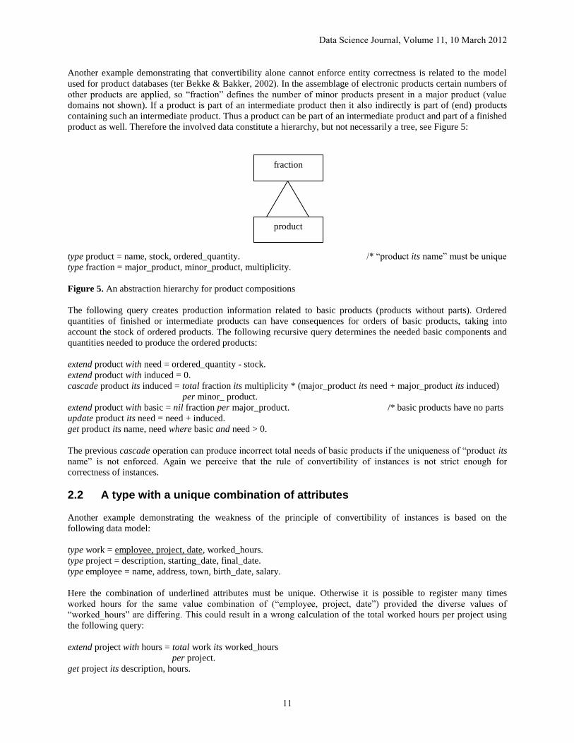
Another example demonstrating that convertibility alone cannot enforce entity correctness is related to the model

used for product databases (ter Bekke & Bakker, 2002). In the assemblage of electronic products certain numbers of

other products are applied, so “fraction” defines the number of minor products present in a major product (value

domains not shown). If a product is part of an intermediate product then it also indirectly is part of (end) products

containing such an intermediate product. Thus a product can be part of an intermediate product and part of a finished

product as well. Therefore the involved data constitute a hierarchy, but not necessarily a tree, see Figure 5:

type product = name, stock, ordered_quantity. /* “product its name” must be unique

type fraction = major_product, minor_product, multiplicity.

Figure 5. An abstraction hierarchy for product compositions

The following query creates production information related to basic products (products without parts). Ordered

quantities of finished or intermediate products can have consequences for orders of basic products, taking into

account the stock of ordered products. The following recursive query determines the needed basic components and

quantities needed to produce the ordered products:

extend product with need = ordered_quantity - stock.

extend product with induced = 0.

cascade product its induced = total fraction its multiplicity * (major_product its need + major_product its induced)

per minor_ product.

extend product with basic = nil fraction per major_product. /* basic products have no parts

update product its need = need + induced.

get product its name, need where basic and need > 0.

The previous cascade operation can produce incorrect total needs of basic products if the uniqueness of “product its

name” is not enforced. Again we perceive that the rule of convertibility of instances is not strict enough for

correctness of instances.

2.2 A type with a unique combination of attributes Another example demonstrating the weakness of the principle of convertibility of instances is based on the

following data model:

type work = employee, project, date, worked_hours.

type project = description, starting_date, final_date.

type employee = name, address, town, birth_date, salary.

Here the combination of underlined attributes must be unique. Otherwise it is possible to register many times

worked hours for the same value combination of (“employee, project, date”) provided the diverse values of

“worked_hours” are differing. This could result in a wrong calculation of the total worked hours per project using

the following query:

extend project with hours = total work its worked_hours

per project.

get project its description, hours.

fraction

product


11

In a relational system based on the data definition: relation work (work#, emp#, proj#, date, worked_hours), this

problem can be solved by using the SQL statement “UNIQUE (emp#, proj#, date)” in the table definition. Another

solution is to define a composite primary key consisting of three attributes (underlined), including two foreign keys

(in italic type face): relation work (emp#, proj#, date, worked_hours).

2.3 Convertibility and externally controlled identifiers The examples in Sections 2.1 and 2.2 discussed identifying attributes with values controllable by a private

organization. Another problem emerges if a commercial organization uses an externally controlled identifier as

identifier. This is illustrated by the following model in which “employee its sofi number” is a unique social

security/fiscal number assigned by the Dutch government to persons (today called “BSN”: “Burger Service

Number”). This number facilitates the work of governmental organizations such as tax offices and passport offices:

type employee = name, address, town, birth_date, sofi number. /* uniqueness over the underlined attributes

type work = description, employee, first_date, last_date.

In order to avoid a conflict with the convertibility of instances, a database designer could choose this sofi number as

an identifier for instances of “employee”, which would result in the following definition in which “sofi number” is

not visible anymore as an attribute:

type employee = name, address, town, birth_date.

However, this identifier (the value of an instance of “employee” equals a sofi number) is controlled by the Dutch

government, and it cannot be excluded that some future government might wish to modify all sofi numbers. This

would create a lot of work in governmental and private databases using sofi numbers as identifiers, especially when

“employee” also functions in a referring attribute such as “work its employee”. In order to avoid this, a sofi number

has to be specified as an identifying property (attribute). The combination of the other attributes (“name, address,

town, birth_date”) constitutes a second identifying property. Now we want to be able to specify the following two

identifying properties: (“employee its sofi number”) and (“employee its name, address, town, birth_date”).

We see that also in the case of an externally controlled identifying attribute, convertibility of instances is not a

usable criterion for entity correctness, and in this example we have to specify two identifying properties.

3 CONVERTIBILITY AND DISJOINT SPECIALIZATION Disjoint specialization occurs when a generalization has two or more non-overlapping specializations (see Section

3.2). These specializations are different in terms of some properties, but their common properties define a

generalization. It is also possible that a generalization is accompanied by only one specialization (Section 3.1). In

theory we might distinguish optional (Sections 3.1 and 3.2) and mandatory specialization (Section 3.3). However,

mandatory single specialization makes no sense: a better design is to merge the definitions of generalization and

specialization type into a single type.

3.1 Optional single specialization

An example of optional single specialization (Figure 6) is related to a building firm offering different standard

houses with or without a dormer. In this firm a house is called a villa if it has a dormer and its number of floors is

larger than two. Now we consider “dormer_width” as property of the specialization “villa”. Both types have in

common the properties included in the definition of the generalization “house”. Table 5 shows some instances of

“house” and “villa”.


12

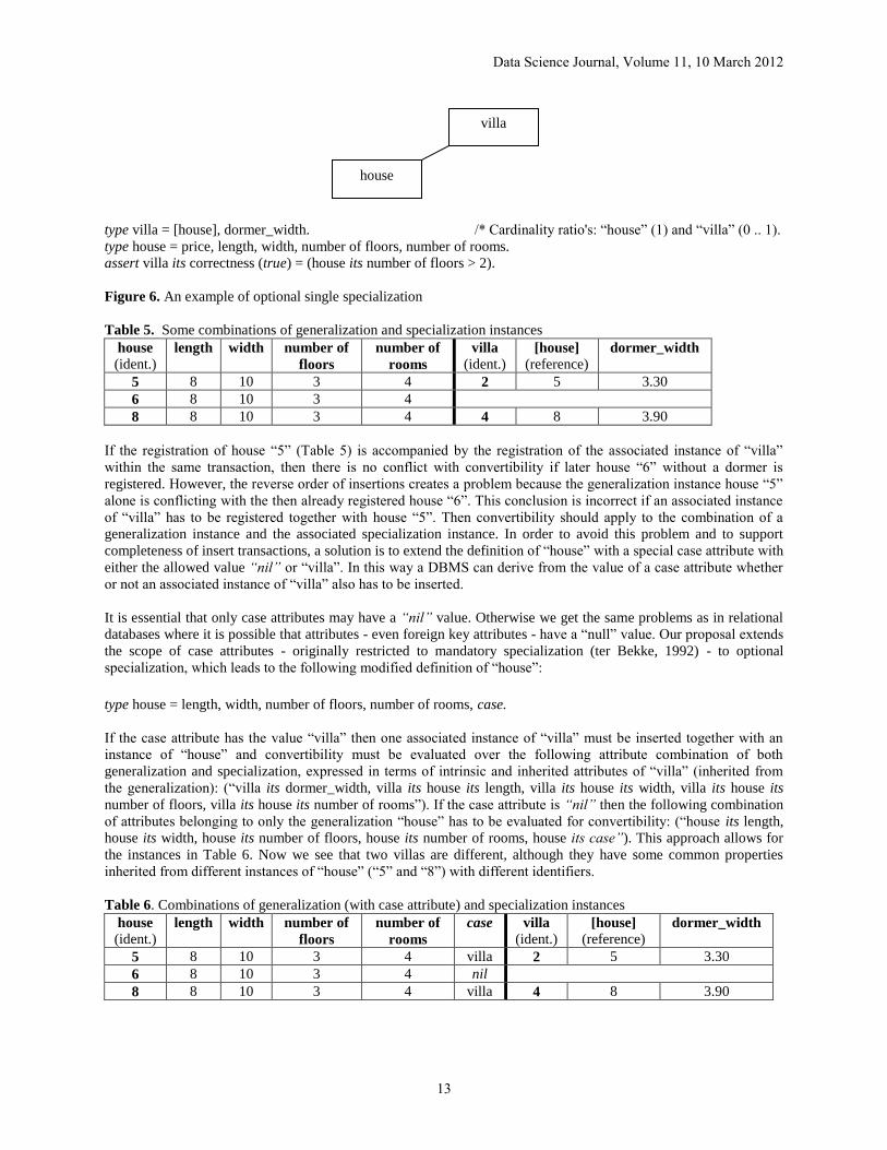
type villa = [house], dormer_width. /* Cardinality ratio's: “house” (1) and “villa” (0 .. 1).

type house = price, length, width, number of floors, number of rooms.

assert villa its correctness (true) = (house its number of floors > 2).

Figure 6. An example of optional single specialization

Table 5. Some combinations of generalization and specialization instances

house

(ident.) length width number of

floors

number of

rooms

villa

(ident.) [house]

(reference) dormer_width

5 8 10 3 4 2 5 3.30

6 8 10 3 4

8 8 10 3 4 4 8 3.90

If the registration of house “5” (Table 5) is accompanied by the registration of the associated instance of “villa”

within the same transaction, then there is no conflict with convertibility if later house “6” without a dormer is

registered. However, the reverse order of insertions creates a problem because the generalization instance house “5”

alone is conflicting with the then already registered house “6”. This conclusion is incorrect if an associated instance

of “villa” has to be registered together with house “5”. Then convertibility should apply to the combination of a

generalization instance and the associated specialization instance. In order to avoid this problem and to support

completeness of insert transactions, a solution is to extend the definition of “house” with a special case attribute with

either the allowed value “nil” or “villa”. In this way a DBMS can derive from the value of a case attribute whether

or not an associated instance of “villa” also has to be inserted.

It is essential that only case attributes may have a “nil” value. Otherwise we get the same problems as in relational

databases where it is possible that attributes - even foreign key attributes - have a “null” value. Our proposal extends

the scope of case attributes - originally restricted to mandatory specialization (ter Bekke, 1992) - to optional

specialization, which leads to the following modified definition of “house”:

type house = length, width, number of floors, number of rooms, case.

If the case attribute has the value “villa” then one associated instance of “villa” must be inserted together with an

instance of “house” and convertibility must be evaluated over the following attribute combination of both

generalization and specialization, expressed in terms of intrinsic and inherited attributes of “villa” (inherited from

the generalization): (“villa its dormer_width, villa its house its length, villa its house its width, villa its house its

number of floors, villa its house its number of rooms”). If the case attribute is “nil” then the following combination

of attributes belonging to only the generalization “house” has to be evaluated for convertibility: (“house its length,

house its width, house its number of floors, house its number of rooms, house its case”). This approach allows for

the instances in Table 6. Now we see that two villas are different, although they have some common properties

inherited from different instances of “house” (“5” and “8”) with different identifiers.

Table 6. Combinations of generalization (with case attribute) and specialization instances

house

(ident.) length width number of

floors

number of

rooms

case villa

(ident.) [house]

(reference) dormer_width

5 8 10 3 4 villa 2 5 3.30

6 8 10 3 4 nil

8 8 10 3 4 villa 4 8 3.90

villa

house


13

Now a case attribute must be involved in the assertions dealing with the completeness of insertions of instances of

“house”. The evaluation order of interdependent assertions can be derived from the position or role of a derivable

variable in an assertion (Bakker &ter Bekke, 2001). This is demonstrated by the following assertions dealing with

the completeness of instances of “house”: the derivable attribute “house its has a dormer” has to be specified before

it can be applied in the second assertion:

assert house its has a dormer = any villa per house.

assert house its completeness (true) = (case = “nil” and not has a dormer or case = “villa” and has a dormer).

If necessary, the DBMS must inform the involved user about the violation of the last rule and advise the user what to

do. Deletion completeness is supported by maintaining referential integrity: a generalization instance may only be

removed after removing all the (specialization) instances referring to that generalization instance. Contrary to this

example with “house” and “villa”, the following sections will show again that convertibility of instances is not

always rigorous enough as a criterion for entity correctness.

3.2 Optional multiple disjoint specialization

A generalization may be accompanied by two or more non-overlapping specializations and each generalization

instance is accompanied by at most one instance of one of the specializations. This means an optional 1 : 1

relationship between an instance of the generalization and an associated instance of one of the specializations.

Therefore the related abstraction hierarchy only shows one line from a block of specializations to the rectangle

representing the generalization. An example is the following data model (Figure 7) for a real estate agency offering

different kinds of buildings for rent (ter Bekke, 1992). We assume that the destination of a building (house or office)

is not predestined. Therefore the specialization of “building” into “house” or “office” is optional.

A block with two specializations:

type office = [building], office type, floor space.

type house = [building], sort, number of rooms.

type building = address, construction_year, purchase_date, price, owner, case.

Figure 7. An example of an abstraction hierarchy for optional multiple disjoint specialization

Disjoint specializations have the same (possibly empty) prefix in the attribute referring to the generalization. These

specializations are not overlapping: they belong to the same block of specializations.

Now “building its case” must be either “nil”, “house”, or “office”. Depending on the actual value, a DBMS has to

decide which kind of instance(s) must be registered within one insert transaction and over which instance(s)

convertibility must be checked. However, a stricter rule for entity correctness has to be specified here because the

following combination of attributes (“building its address, building its construction_year”) must be unique: this

combination is an identifying property of “building” and also is an inherited identifying property of both

specializations (via “office its building” or “house its building”). For example, the identifying property of “house”

can be specified as: (“house its building its address, house its building its construction_year”). Completeness of

building registrations can be enforced by using the following assertions:

assert building its is office = any office per building. /* Definition and calculation of a derived attribute.

assert building its is house = any house per building. /* Idem.

assert building its completeness (true) = (case = “nil” and not is office and not is house

or case = “house” and is house or case = “office” and is office).

office

house

building


14

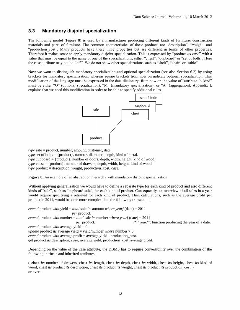
3.3 Mandatory disjoint specialization The following model (Figure 8) is used by a manufacturer producing different kinds of furniture, construction

materials and parts of furniture. The common characteristics of these products are “description”, “weight” and

“production_cost”. Many products have these three properties but are different in terms of other properties.

Therefore it makes sense to apply mandatory disjoint specialization. This is expressed by “product its case” with a

value that must be equal to the name of one of the specializations, either “chest”, “cupboard” or “set of bolts”. Here

the case attribute may not be “nil”. We do not show other specializations such as “shelf”, “chair” or “table”.

Now we want to distinguish mandatory specialization and optional specialization (see also Section 6.2) by using

brackets for mandatory specialization, whereas square brackets from now on indicate optional specialization. This

modification of the language must be expressed in the data dictionary: from now on the value of “attribute its kind”

must be either “O” (optional specialization), “M” (mandatory specialization), or “A” (aggregation). Appendix I.

explains that we need this modification in order to be able to specify additional rules.

type sale = product, number, amount, customer, date.

type set of bolts = {product}, number, diameter, length, kind of metal.

type cupboard = {product}, number of doors, depth, width, height, kind of wood.

type chest = {product}, number of drawers, depth, width, height, kind of wood.

type product = description, weight, production_cost, case.

Figure 8. An example of an abstraction hierarchy with mandatory disjoint specialization

Without applying generalization we would have to define a separate type for each kind of product and also different

kinds of “sale”, such as “cupboard sale”, for each kind of product. Consequently, an overview of all sales in a year

would require specifying a retrieval for each kind of product. Then calculations, such as the average profit per

product in 2011, would become more complex than the following transaction:

extend product with yield = total sale its amount where yearf (date) = 2011

per product.

extend product with number = total sale its number where yearf (date) = 2011

per product. /* “yearf”: function producing the year of a date.

extend product with average yield = 0.

update product its average yield = yield/number where number > 0.

extend product with average profit = average yield - production_cost.

get product its description, case, average yield, production_cost, average profit.

Depending on the value of the case attribute, the DBMS has to require convertibility over the combination of the

following intrinsic and inherited attributes:

(“chest its number of drawers, chest its length, chest its depth, chest its width, chest its height, chest its kind of

wood, chest its product its description, chest its product its weight, chest its product its production_cost”)

or over:

set of bolts

cupboard

sale chest

product


15

(“cupboard its number of doors, cupboard its depth, cupboard its width, cupboard its height, cupboard its kind of

wood, cupboard its product its description, cupboard its product its weight, cupboard its product its

production_cost”)

or over:

(“set of bolts its number, set of bolts its diameter, set of bolts its length, set of bolts its kind of metal, set of bolts its

product its description, set of bolts its product its weight, set of bolts its product its production_cost”).

Each of these attribute combinations is suitable as identifying property for the involved specialization. Now the

generalization “product” does not need to have any identifying property. However, this is not a general rule for all

cases with mandatory specialization. This is demonstrated by the data model in Figure 9, a slight modification of an

example in the textbook (ter Bekke, 1992). It is related to a banking organization with regional head offices and

branches, each branch reporting to a head office. This organization requires that an office is either a branch or a head

office: therefore the value of “office its case” must be either “head office” or “branch”.

type head office = [office], region.

type branch = [office], head office.

type office = address, town, telephone number, case.

Figure 9. Another example of mandatory disjoint specialization

Two attributes of the generalization (“office its address” and “office its town”) constitute an identifying property and

“office its telephone number” is another identifying property. It makes sense that the specializations inherit the

identifying properties of their generalization. For example, the identifying properties of “branch” are defined by

(“branch its office its address, branch its office its town”) and (“branch its office its telephone number”).

In the case of mandatory specialization there is no need to specify any identifying property for the generalization.

Even if attributes of a generalization alone or together with attributes of an associated specialization are participating

in an identifying property of a specialization, the specialization and not the generalization must have at least one

identifying property, possibly containing an attribute inherited from the generalization. Another choice is possible,

but a generic solution requires applying a standard approach to all cases with mandatory specialization. Section 6.2

will show that this is essential for checking correctness of specifications.

4 CONVERTIBILITY AND NON-DISJOINT SPECIALIZATION In the case of non-disjoint or overlapping specialization there are at least two specialization blocks and each block

consists of at least one specialization. Then each instance of a generalization may be accompanied by many

specialization instances if these instances belong to different blocks. Each block must be identified by a unique

prefix in the attribute referring from a specialization to a generalization. Two variants of non-disjoint specialization

are possible: optional and mandatory. However, the last kind is superfluous because a more usable design is to

merge the attributes of the specializations with the attributes of the generalization into a single composite type.

4.1 Optional non-disjoint specialization An example (Figure 10) of optional non-disjoint specialization is related to a school with three categories of

employees: common employees without any specific characteristics, or employees with specific characteristics:

teachers and/or managers. We assume that in this school a teacher may also be a manager at the same time:

head office

office

branch


16

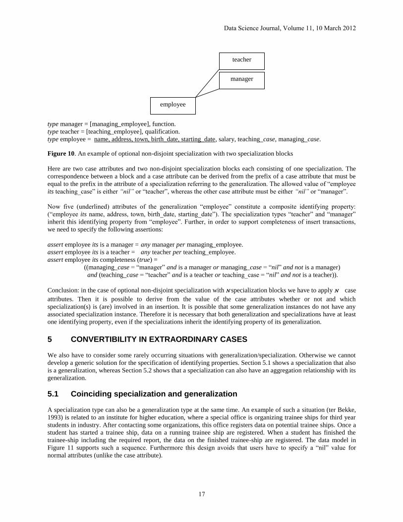
type manager = [managing_employee], function.

type teacher = [teaching_employee], qualification.

type employee = name, address, town, birth_date, starting_date, salary, teaching_case, managing_case.

Figure 10. An example of optional non-disjoint specialization with two specialization blocks

Here are two case attributes and two non-disjoint specialization blocks each consisting of one specialization. The

correspondence between a block and a case attribute can be derived from the prefix of a case attribute that must be

equal to the prefix in the attribute of a specialization referring to the generalization. The allowed value of “employee

its teaching_case” is either “nil” or “teacher”, whereas the other case attribute must be either “nil” or “manager”.

Now five (underlined) attributes of the generalization “employee” constitute a composite identifying property:

(“employee its name, address, town, birth_date, starting_date”). The specialization types “teacher” and “manager”

inherit this identifying property from “employee”. Further, in order to support completeness of insert transactions,

we need to specify the following assertions:

assert employee its is a manager = any manager per managing_employee.

assert employee its is a teacher = any teacher per teaching_employee.

assert employee its completeness (true) =

((managing_case = “manager” and is a manager or managing_case = “nil” and not is a manager)

and (teaching_case = “teacher” and is a teacher or teaching_case = “nil” and not is a teacher)).

Conclusion: in the case of optional non-disjoint specialization with N specialization blocks we have to apply N case

attributes. Then it is possible to derive from the value of the case attributes whether or not and which

specialization(s) is (are) involved in an insertion. It is possible that some generalization instances do not have any

associated specialization instance. Therefore it is necessary that both generalization and specializations have at least

one identifying property, even if the specializations inherit the identifying property of its generalization.

5 CONVERTIBILITY IN EXTRAORDINARY CASES

We also have to consider some rarely occurring situations with generalization/specialization. Otherwise we cannot

develop a generic solution for the specification of identifying properties. Section 5.1 shows a specialization that also

is a generalization, whereas Section 5.2 shows that a specialization can also have an aggregation relationship with its

generalization.

5.1 Coinciding specialization and generalization

A specialization type can also be a generalization type at the same time. An example of such a situation (ter Bekke,

1993) is related to an institute for higher education, where a special office is organizing trainee ships for third year

students in industry. After contacting some organizations, this office registers data on potential trainee ships. Once a

student has started a trainee ship, data on a running trainee ship are registered. When a student has finished the

trainee-ship including the required report, the data on the finished trainee-ship are registered. The data model in

Figure 11 supports such a sequence. Furthermore this design avoids that users have to specify a “nil” value for

normal attributes (unlike the case attribute).

teacher

manager

employee


17

type finished traineeship = [running traineeship], report_title, final_date, mark, reviewer.

type running traineeship = [traineeship], start_date, planned final_date, case.

type traineeship = organization, contact person, telephone, subject, desired start_date, desired final_date, case.

Figure 11. A data model for the registration of traineeships

Further, some additional restrictions are essential:

init default traineeship its case = “nil”. /* update case when inserting an instance of “running traineeship”

init default running traineeship its case = “nil”. /* update case when inserting an instance of “finished traineeship”

assert running traineeship its is finished = any finished traineeship

per running traineeship.

assert traineeship its is running = any running traineeship where not is finished

per traineeship.

assert traineeship its completeness (true) = (case = “nil” and not is running

or case = “running traineeship” and is running).

assert running traineeship its completeness (true) = (case =“nil” and not is finished

or case = “finished traineeship” and is finished).

The following attribute combination of “traineeship” constitutes an identifying property: (“organization, subject,

desired start_date”). The types “running traineeship” and “finished traineeship” inherit this identifying property.

The first specialization inherits this identifying property via the path “running traineeship its traineeship”, whereas

the second specialization inherits this identifying property via “finished traineeship its running traineeship its

traineeship”. For example, one of the inherited attributes can be specified as “finished traineeship its running

traineeship its traineeship its subject”. In this case both generalization and specializations must have at least one

identifying property because it is possible that an instance of a generalization (“traineeship” or “running

traineeship”) is not accompanied by any following specialization instance.

5.2 Simultaneous aggregation and specialization of a same type The situation mentioned in the previous title occurs in the database of a library in a large governmental organization

where data on reports have to be stored and must be accessible via an index. There are reports commenting on

another report. Now “commentary” is an optional specialization of “report”, but at the same time it is also based on

an aggregation with the same type “report” because it comments on a previous report. Further, at least one author is

responsible for a chapter of a report. Figure 12 shows an abstraction hierarchy for this index. The definition of the

composite type “department” is not shown because its attributes are irrelevant for the present discussion.

running

traineeship

finished

traineeship

traineeship


18

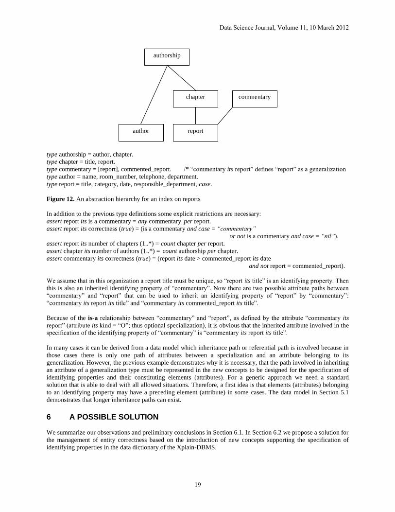
type authorship = author, chapter.

type chapter = title, report.

type commentary = [report], commented_report. /* “commentary its report” defines “report” as a generalization

type author = name, room_number, telephone, department.

type report = title, category, date, responsible_department, case.

Figure 12. An abstraction hierarchy for an index on reports

In addition to the previous type definitions some explicit restrictions are necessary:

assert report its is a commentary = any commentary per report.

assert report its correctness (true) = (is a commentary and case = “commentary”

or not is a commentary and case = “nil”).

assert report its number of chapters (1..*) = count chapter per report.

assert chapter its number of authors (1..*) = count authorship per chapter.

assert commentary its correctness (true) = (report its date > commented_report its date

and not report = commented_report).

We assume that in this organization a report title must be unique, so “report its title” is an identifying property. Then

this is also an inherited identifying property of “commentary”. Now there are two possible attribute paths between

“commentary” and “report” that can be used to inherit an identifying property of “report” by “commentary”:

“commentary its report its title” and “commentary its commented_report its title”.

Because of the is-a relationship between “commentary” and “report”, as defined by the attribute “commentary its

report” (attribute its kind = “O”; thus optional specialization), it is obvious that the inherited attribute involved in the

specification of the identifying property of “commentary” is “commentary its report its title”.

In many cases it can be derived from a data model which inheritance path or referential path is involved because in

those cases there is only one path of attributes between a specialization and an attribute belonging to its

generalization. However, the previous example demonstrates why it is necessary, that the path involved in inheriting

an attribute of a generalization type must be represented in the new concepts to be designed for the specification of

identifying properties and their constituting elements (attributes). For a generic approach we need a standard

solution that is able to deal with all allowed situations. Therefore, a first idea is that elements (attributes) belonging

to an identifying property may have a preceding element (attribute) in some cases. The data model in Section 5.1

demonstrates that longer inheritance paths can exist.

6 A POSSIBLE SOLUTION We summarize our observations and preliminary conclusions in Section 6.1. In Section 6.2 we propose a solution for

the management of entity correctness based on the introduction of new concepts supporting the specification of

identifying properties in the data dictionary of the Xplain-DBMS.

authorship

chapter

commentary

author

report


19

6.1 Rules for entity correctness

The discussions in Sections 2-5 lead us to the following conclusions:

1. Each instance of a composite type must have a unique single valued identifier that may not be modified, which

complies with the original concepts of Xplain.

2. According to the original concepts of Xplain convertibility of instances should be checked over the

combination of a generalization instance and the associated specialization instance(s).

3. If a type is neither generalization nor specialization then convertibility of instances is required for that type.

4. However, rule 2 and rule 3 must be ignored if stricter uniqueness rules for entity correctness are required.

If a type is neither generalization nor specialization then uniqueness should be specified over some of its

attributes. An example is the composite type “department” with two identifying properties (Section 2).

For situations with optional specialization it is necessary to define for both the generalization and its

specializations at least one identifying property because the case attribute may be “nil”, indicating there is not

any specialization instance. A specialization may inherit this identifying property from its generalization (for

example, in Section 3.2 “house” and “office” inherit from “building”), or a specialization may have its own

identifying property defined over its intrinsic and inherited attributes (for example, “villa” in Section 3.1).

In situations with mandatory specialization only the specializations must have at least one identifying property

because an instance of a generalization with mandatory specialization may not exist without any associated

specialization instance. Still it is possible that specializations inherit an identifying property of their

generalization (for example: “branch” and “head office” inherit from their generalization “office”).

5. In order to support database transactions for the insertion of a generalization instance together with the possibly

associated specialization instance(s), we propose to apply case attributes for mandatory and optional

specialization as well. The value of a case attribute may be “nil” or equal to the name of an associated

specialization type in the case of optimal specialization. However, in the case of mandatory specialization, this

value must be equal to the name of the associated specialization type.

The actually required rules must be dealt with by the diverse subsystems of the Xplain-DBMS such as query

interpreter and application generator. For example, the generator supports the design of correctly nested structures

consisting of visible window fields for a generalization instance together with window fields for associated

specialization instance(s) (ter Bekke, 1994, 1995). This application generator is also able to support the presentation

of warnings about involved rules and other information.

6.2 Concepts for the specification of identifying properties We demonstrated that convertibility of instances is not always rigorous enough a criterion for entity correctness. In

order to design a generic solution for this weakness we require that identifying properties must always be specified

explicitly, even when convertibility of instances is a satisfactory correctness requirement. Furthermore, each

composite type must have at least one identifying property, except that generalizations with mandatory

specialization do not need to have any identifying property. In the last case only the specializations must have at

least one identifying property. An identifying property of a specialization type may be based on its intrinsic

attributes and attributes inherited from its generalization.

In order to be able to register identifying properties and their constituting elements in a data dictionary we have to

design new concepts such as “identifying property” and “element” in addition to the modeling concepts “type”,

“attribute” and “role attribute”. An identifying property has to refer to a composite type without mandatory

specialization and also must have a unique name because more than one identifying property per type is possible.

Further, an identifying property must be based on at least one attribute (an element of the identifying property).

Because it is possible that an identifying property is based on many attributes an element must refer to an identifying

property and to an intrinsic attribute or an attribute inherited from its generalization. So there is a 1 : n cardinality

ratio (n > 0) between “identifying property” and “element”.

It is possible that a specialization has two references to its generalization (see the example in Section 5.2 with the

types “commentary” and “report”) and inherits the identifying property of its generalization. Therefore it is


20

necessary for a generic solution that an inheritance path via a series of elements can be specified. This leads to the

following definition of new concepts for a data dictionary:

type identifying property = name, involved_type. /* unique name

type element = attribute, preceding_element, identifying property.

The concept of “element” refers to itself via “element its preceding_element”. Similar recursive structures are also

an essential part of meta models for data distribution and parallel input/output in database management systems

(Bakker, 1994, 1998, 2000).

The original concepts of Xplain required that the value of “attribute its kind” must be either “A” (aggregation) or

“G” (generalization/specialization). Then it was possible to derive from the value “G” and the simultaneous

presence of a case attribute that mandatory specialization was meant. However, since we extended the scope of case

attributes to optional specialization in order to support completeness of insert transactions, this derivation can no

longer be applied. In order to solve this problem, we introduced in Section 3.3 two different values “O” and “M” for

“attribute its kind” indicating either optional (“O”) or mandatory specialization (“M”).

In the case of “O” the generalization must have at least one identifying property, whereas “M” implies that the

generalization needs not to have any identifying property. In this way it becomes possible to specify a generic rule

indicating which types must have at least one identifying property. Examples with optional specialization are the

generalizations “house” (specialization: “villa”), “building” (specializations: “house” and “office”) and “employee”

(specializations: “manager” and “teacher”). This consideration leads us to the extended meta model for the data

dictionary of Xplain, shown in Figure 13.

type element = attribute, preceding_element, identifying property.

type identifying property = name, involved_type. /* unique name

type role attribute = [attribute], prefix.

type attribute = composite_type, type, kind.

type type = name, representation. /* unique name

Figure 13. Extended meta model for the Xplain data dictionary

The following assertions are needed for later discussed transactions checking correctness of a data model. They

cannot interfere with the insertion of any instance because these assertions do not contain any value restriction:

assert type its composite = any attribute

per composite_type.

assert type its has optional specialization = any attribute where kind = “O”

element

identifying

property

attribute

role attribute

type


21

per type.

assert type its has mandatory specialization = any attribute where kind = “M”

per type.

assert type its is a generalization = (has optional specialization or has mandatory specialization).

assert type its is a specialization = any attribute where kind = “O” or kind = “M”

per composite_type.

assert type its number of case attributes = count attribute where type its name = “case”

per composite_type.

assert type its has optional non-disjoint specialization = (number of case attributes > 1).

assert attribute its prefix = some role attribute its prefix

per attribute.

The some function produces a single random result (an empty result is specified as “void”). However, in this case

this single result can only be a prefix or “void” because there is at most one role attribute per attribute.

Many correctness checks are required because not all required rules are inherent in the meta model. These checks

can be specified in terms of assertions, but then some assertions will be triggered during the specification of types

and attributes. For example, the following assertion for “type its correctness”, dealing with the required minimal

number of identifying properties per type, is triggered by the insertion of a new type and could require some

additional insertions in the case of some composite types:

assert type its number = count identifying property

per involved_type.

assert type its correct (true) = (composite and (not is a generalization and not is a specialization and number ≥ 1

or has optional specialization and number ≥ 1 or has mandatory specialization and number = 0

or is a specialization and number ≥ 1) or not composite and number = 0).

In order to prevent this interference during the specification of a data model it is better to separate concerns, thus to

use checking transactions that must be executed by a database administrator after completing the registration of all

types, attributes and role attributes. We can distinguish four main tasks for such checking transactions:

1. Checking the correctness of a data model.

For example, in the case of generalization/specialization each specialization block is identified by the prefix in

the attribute referring from a specialization to the generalization. It is required that the same prefix is applied in

the involved case attribute.

2. Checking the required minimal number of identifying properties.

Each composite type must have at least one identifying property, but in the case of mandatory specialization

the generalization needs not to have any identifying property.

3. Checking the required minimal number of elements.

Each identifying property must have at least one element (based on an attribute) referring to that identifying

property.

4. Checking the correctness of elements.

The recursive definition of the concept “element” as such does not enforce that a sequence of elements is

correctly specified, so a check for correctness is necessary.

We can specify the required checks in the language of Xplain or we describe them. Because of the structure of the

extended meta model it makes sense to register meta data and check their correctness in the following order:

1. Data model (types, attributes and role attributes),

2. Identifying properties (they refer to a composite type) and

3. Elements (they refer to an identifying property).

The required checking transactions will be discussed extensively in Appendix I.


22

7 DISCUSSION

One principle in Xplain databases remains unchanged: each instance of a composite type has a single, unmodifiable

identifier. This is an essential difference with the relational language SQL that allows for a composite primary key

even when consisting of modifiable attributes (Connolly, Begg, & Strachan, 1995). A modification of such a key can

lead to time consuming consequences for data management, especially when a modifiable primary key is referenced

by a foreign key in another relation.

Although convertibility of instances is not an incorrect criterion for uniqueness of instances, it is not always a

satisfactory correctness criterion for instances. In Section 2.2 the example based on Figure 1 showed that incorrect

instances can lead to derivations producing wrong results. The same problem can occur in the case of recursive

calculations (Section 2.1). Aiming at a generic standard solution, stricter rules for correctness of instances should be

specified in terms of identifying properties, even if convertibility of instances happens to be a satisfactory criterion

for correctness of instances. Therefore we introduced new concepts supporting the specification of identifying

properties and their constituting elements. Correctness of these data can be supported by checking transactions if the

following standard solution is applied:

Each composite type must have at least one identifying property. The only exception is that a mandatory

generalization need not have any identifying property (examples: the furniture case with “product” and the bank

case with “office”, both in Section 3.3). In this standard solution it is even possible (see the bank case) that a

specialization inherits an identifying property from its generalization. However, if a composite type has more than

one identifying property, it is the responsibility of a database designer to specify all required identifying properties.

An alternative is to use the same proposed meta model without applying the proposed standard solution. In many

cases it is sufficient to specify an identifying property for only a generalization. For example, if we specify an

identifying property for the generalization “building” (specializations: “house” and “office”), then there is no need

to specify any identifying property for the specializations. However, such ad hoc choices cannot be checked for

correctness by predefined transactions because they do not comply with the described standard solution. Allowing

such ad hoc decisions would imply a heavier burden for a database designer.

Berend de Boer and Johan ter Bekke (2001) showed that data definitions and queries in Xplain can be transformed

into correct SQL specifications (ter Bekke, 1994, 1995, 1999). Contrary to this conversion, the present paper opens

the possibility for a reverse transformation, which is very important considering the large number of existing

relational databases. The Xplain-DBMS has a facility to import records from other databases (ter Bekke, 1998). If

the relational data have a composite primary key, then Xplain can automatically generate the single identifier for

each instance to be inserted. However, it probably is better to execute other modifications (corrections) in the

relational database itself, in particular because of the need to check for referential integrity. Possible complications

are: foreign keys with a “null” value or foreign keys consisting of many attributes, to be replaced by a single foreign

key. The advantage obtained by such a transformation is that the Xplain language can be used. This language is

more suitable for end user computing than SQL because in Xplain join operations and nested queries need not and

cannot be specified, which is also important for database security. For example, in many cases security holes can be

attributed to improperly formed SQL queries (North, 2010). We have demonstrated (ter Bekke, 1997; Bakker & ter

Bekke, 2001) that the Xplain language is better and simpler structured than SQL, which makes it easier to prevent

improperly specified queries. This is extremely important in open systems accessible via the Internet.

Unfortunately, the extension of Xplain with recursive operations was the last main improvement Johan ter Bekke

was able to implement. Considering the strict dependency between data manipulation and data structure in the

Xplain-DBMS - also in the case of recursive operations - we may consider his work as an essential contribution to

the field of database management systems but also to end user computing. Moreover, his work also demonstrates

that query-functionality is limited by data structure as defined by a data model. The present paper has shown that in

many cases - with or without generalization/specialization - convertibility of instances is not a satisfactory

requirement for correctness of instances and that additional uniqueness rules - using identifying properties - have to

be applied in order to guarantee that (recursive) calculations in queries produce correct results.


23

8 ACKNOWLEDGEMENT The author would like to thank the reviewers and also Berend de Boer and Martin van Dinther for their valuable

comments on earlier versions of the present paper.

9 REFERENCES

Aho, A.V., Hopcroft, J.E., & Ullman, J.D. (1974) The Design and Analysis of Computer Algorithms, Addison-

Wesley, Reading (MA), p. 208.

Bailey, D.A. (1999) Java structures: Data structures in JAVA for the principled programmer, MacGraw-Hill,

Boston, USA.

Bakker, J.A. (1994) A semantic approach to enforce correctness of data distribution schemes, The Computer Journal

37 (7), pp. 561-575.

Bakker, J.A. (1998) An extended meta model for conditional fragmentation, Proceedings 9th

International

Conference on Database and Expert Systems Applications DEXA’98, Vienna, Austria, Eds. Quirchmayr, G.,

Schweighofer, E. & Bench-Capon, T.J.M., Lecture Notes in Computer Science 1460, pp. 702-715.

Bakker, J.A. (2000) A semantic framework for the design of data distribution schemes, Proceedings 11th

International Workshop on Database and Expert Systems Applications, Greenwich, London, UK, Eds. Tjoa, A.M.,

Wagner, R.R. & Al-Zobaidie, A., pp. 653-660.

Bakker, J.A. (2000) Semantic partitioning as a basis for parallel I/O in database management systems, Parallel

Computing 26, pp. 1491-1513.

Bakker, J.A. & Bekke, J.H. ter (2001) Maintaining derived information using dynamic rule ordering, Proceedings

International Conference on Intelligent Systems and Control (ICSC 2001), Clearwater, Florida, Ed. Hamza, M.H.,

pp. 253-260.

Bakker, Bert & Bekke, J. H. ter (2001) Foolproof query access to search engines, Proceedings Third International

Conference on Information Integration and Web-based Applications & Services (IIWAS 2001), Linz, Austria, Eds.

Winiwarter, W., St. Bressan, St. & Ibrahim, I.K., pp. 389 - 394.

Bakker, J.A. & Bekke, J.H. ter (2002) Efficient maintenance of derived information in active databases, Proceedings

6th

International Conference on Artificial Intelligence and Soft Computing, Bannf, Canada, Ed. Leung, H., pp. 118-

122.

Bakker, J.A. & Bekke, J.H. ter (2004) A query language solution for fastest flight connections, Proceedings

IASTED International Conference on Databases and Applications, Innsbruck, Austria, Ed. Hamza, M.H., pp. 197-

202.

Bakker, J.A. & Bekke, J.H. ter (2004) A query language solution for shortest path problems in cyclic geometries,

Proceedings IASTED International Conference on Databases and Applications, Innsbruck, Austria, Ed. Hamza,

M.H., pp. 203-207.

Bancilhon, F. & Ramakrishnan, R. (1986) An amateur’s introduction to recursive query processing strategies,

Proceedings 1986 ACM SIGMOD International Conference on Management of Data, Washington D.C., USA, pp.

16-52.

Bang-Jensen, J. & Gutin, G. (2001) Digraphs: Theory, Algorithms and Applications, Springer-Verlag, London, UK.

Bekke, J.H. ter (1980) Convertibility in databases, Information Processing Letters 11, number 4/5 (December 12),

pp. 168-171.


24

Bekke, J.H. ter (1983) Database Ontwerp, Stenfert Kroese, Leiden, the Netherlands (in Dutch).

Bekke, J.H. ter (1991) Semantic data modeling in relational environments, doctoral thesis, Delft University of

Technology, Delft, the Netherlands.

Bekke, J.H. ter (1992) Semantic Data Modeling, Prentice Hall International, Hemel Hempstead, UK.

Bekke, J.H. (1993) Database Ontwerp, Kluwer Bedrijfswetenschappen, Deventer, the Netherlands (in Dutch).

Bekke, J.H. ter (1994) Complex values in databases, Proceedings International Conference on Data and Knowledge

Systems for Manufacturing and Engineering, Hong Kong, Ed. Chen, N., pp. 449-455.

Bekke, J.H. ter (1995) Meta modeling for end user computing, Proceedings Workshop on Database and Expert

Systems Applications DEXA 1995, London, UK, Eds. Revell, N. & Tjoa, A. M., pp. 267-273.

Bekke, J.H. ter (1997) Can we rely on SQL?, Proceedings 8th International DEXA Workshop, Toulouse, France, Ed.

Wagner, R.R., IEEE Computer Society, pp. 378-383.

Bekke, J.H. ter (1997), Advantages of a compact semantic meta model, Proceedings 2nd

IEEE Metadata Conference,

Silver Spring, USA. Retrieved from the World Wide Web, February 11, 2012:

http://www.computer.org/conferen/proceed/meta97/papers/jterbekke/jterbekke.html

Bekke, J.H. ter (1998) Xplain manual (in Dutch), version 5.4, Delft University of Technology, Delft, the

Netherlands (in Dutch).

Bekke, J.H. ter (1999) Semantic requirements for databases in casual environments, Electronic Proceedings of

SAICSIT ‘99: Prepare for the New Millennium, Johannesburg, South Africa, Ed. P. Machanick, pp.1-10.

Bekke, J.H. ter & Bakker, J.A. (2001) Limitations of relationships constructed from coinciding data, Proceedings

International Conference on Intelligent Systems and Control (ICSC 2001), Clearwater, Florida, USA, Ed. Hamza,

M.H., pp. 247 - 252.

Bekke, J.H. ter & Bakker, J.A. (2002) Content-driven Specifications for Recursive Project Planning Applications,

Proceedings IASTED International Conference on Applied Informatics, Innsbruck, Austria, Ed. Hamza, M.H., pp.

448-452.

Bekke, J.H. ter & Bakker, J.A. (2002) Recursive queries in product database, Proceedings 5th

International

Conference on Flexible Query Answering Systems (FQAS 2002), Copenhagen, Denmark, October 27-29, Lecture

Notes in Computer Science (Subseries LNAI) Volume 2522, Eds. Andreasen, T., Motro, A., Christiansen, H. &

Legind Larsen, H., Springer-Verlag, Berlin-Heidelberg, pp. 44-55.

Bekke, J.H. ter & Bakker, J.A. (2003) Modeling and Querying Recursive Data Structures I: Introduction,

Proceedings 7th

International Conference on Artificial Intelligence and Soft Computing, Banff , Canada, Ed. Leung,

H., pp. 278-282.

Bekke, J.H. ter & Bakker, J.A. (2003) Modeling and Querying Recursive data Structures II: A Semantic Approach,

Proceedings 7th

International Conference on Artificial Intelligence and Soft Computing, Banff, Canada, Ed. Leung,

H., pp. 283-289.

Bekke, J.H. ter & Bakker, J.A. (2003) Fast recursive data processing in graphs using reduction, Proceedings

IASTED International Conference on Applied Informatics, Innsbruck, Austria, Ed. Hamza, M.H., pp. 490-494.

Boer, Berend de & Bekke, J.H. ter (2001) Applying semantic database principles in a relational environment,

Proceedings International Symposium Applied Informatics (AI2001), Innsbruck, Austria, Ed. Hamza, M.H., pp. 400-

405.


25

http://www.computer.org/conferen/proceed/meta97/papers/jterbekke/jterbekke.html

Codd, E.F. (1970) A relational model of data for large shared data banks, Communications of the ACM 13, pp. 377-

387.

Connolly, T., Begg, C., & Strachan, A. (1995) Database Systems, A practical approach to design, implementation

and management, 6th

ed., Addison-Wesley, Reading (MA).

Dar, S. & Ramakrishnan, R. (1994) A performance study of transitive closure algorithms, ACM SIGMOD Record,

23, pp. 454-465.

Elmasri, R. & Navathe, S.B. (2010) Fundamentals of Database Systems, 6th

ed., Addison-Wesley.

Karayiannis, A. & Loizou, G. (1978) Cycle detection in critical path networks, Information Processing Letters, 7,

pp. 15-19.

Molluzzo, J.C. (1986) A first course in discrete mathematics, Wadsforth, Belmont CA.

North, K. (2010) Terabytes to Petabytes: Reflections 1999-2009, Dr. Dobb’s, January 4. Retrieved from the World

Wide Web, February 13, 2012: http://drdobbs.com/blogs/architecture-and-design/228701466

Rolland, F. (1998) The essence of databases, Prentice Hall, Hemel Hempstead, UK.

Rosenthal, A., Heder, S., Dayal, U. & Manola, F. (1986), Traversal Recursion: A Practical Approach to Supporting

Recursive Applications, Proceedings ACM SIGMOD International Conference on Management of Data,

Washington D.C., USA, pp. 166-176.

Smith, J.M & Smith, D.C.P. (1977) Database abstractions: aggregation, Communications of the ACM 20, pp. 405-

413.

Smith, J.M. & Smith, D.C.P. (1977) Database abstractions: aggregation and generalization, ACM Transactions on

Database Systems 2, pp. 105-133.

Suciu, D. & Paredaens, J. (1994) Any algorithm in the complex object algebra with power set needs exponential

space to compute transitive closure, Proceedings ACM SIGACT-SIGMOD-SIGART Symposium on Principles of

Database Systems, Minneapolis, Minnesota, USA, pp. 201-209.

Ullman, J.D. & Widom, J. (1997) A first course in Database Systems, Prentice Hall, Hemel Hempstead.

Many of these publications and related work can be found via http://www.jhterbekke.net/publications.html

APPENDIX I

I.1 Checking the correctness of a data model

Some of the required rules (assertions) are already mentioned in relation to Figure 10. It makes sense to check the

underlying data model for correctness. For example, the prefix of a case attribute must be equal to the prefix in an

attribute referring from a specialization to a generalization. Further, for each composite type the number of case

attributes must be equal to the number of specialization blocks. In the case of disjoint specialization the block

number must be one. If a type is not a specialization and also not a generalization then its block number must be

zero. In the case of optional non-disjoint specialization there must be two or more blocks (for example, “employee”

has overlapping specializations “teacher” and “manager”).

extend type with block number = count attribute its prefix where kind = “O” or kind = “M”

per type.

extend type with correct = (number of case attributes = block number


26

http://drdobbs.com/blogs/architecture-and-design/228701466

http://www.jhterbekke.net/publications.html

and has optional specialization and block number = 1 or has mandatory specialization and block number = 1

or has optional non-disjoint specialization and block number > 1

or not is a generalization and not is a specialization and block number = 0)).

get type its name, number of case attributes, block number where composite and not correct.

The prefix in a case attribute must be equal to the prefix in the attribute referring from a specialization to a

generalization:

extend type with block name 1 = some attribute its prefix where kind = “O” or kind = “M”

per type.

extend type with block name 2 = some attribute its prefix

where kind = “O” or kind = “M” and not prefix = type its block name 1

per type.

extend attribute with correct prefix = (type its name = “case” and (prefix = composite_type its block name 1

or prefix = composite_type its block name 2) or not type its name = “case”.

get attribute its composite_type its name where type its name = “case” and not correct prefix.

In a similar way more block names can be copied into derived attributes of a generalization.

I.2 Checking the required minimal number of identifying properties

An identifying property must have a unique name and must be specified through a set of (possibly inherited)

elements. Further, “identifying property its involved_type” must be a composite type. Incorrectly specified

identifying properties are retrieved by:

get identifying property its name, involved_type its name where not involved_type its composite.

It is also required that almost each composite type has at least one identifying property. Only a generalization with

mandatory specialization needs not to have any identifying property:

extend type with number = count identifying property

per involved_type.

extend type with correct = (not is a generalization and not is a specialization and number > 0

or has optional specialization and number > 0 or has mandatory specialization and number = 0

or is a specialization and number > 0 or not composite and number = 0).

get type its name, number of identifying properties where composite and not correct.

However, the number of identifying properties a type must have cannot be derived from a data model. This remains

the responsibility of the involved database designer. An example of a composite type with two identifying properties

is “department” (Section 2, Table 4).

I.3 Checking the required minimal number of elements

The number of elements per identifying property must be at least one:

extend identifying property with number of elements = count element

per identifying property.

get identifying property its name, involved_type its name, number of elements

where number of elements = 0.


27

I.4 Checking the correctness of elements

Elements in a path belong to the same identifying property. Therefore “element its identifying property” must be

equal to “element its preceding_element its identifying property”. This rule does not apply if an element is not

preceded by another element (it is a first or ‘lowest’ element in a path). Then it is necessary to apply a special value

such as “0” for “element its preceding_element”. For example, the element participating in the identifying property

of “chest”, based on the attribute “product its description” (Section 4.3) is not preceded by any element.

For a really existing preceding element, “element its attribute its type” must be equal to “element its

preceding_element its attribute its composite_type”. An example is “chest its product its weight” participating in the

identifying property of “chest”. Here “chest its product” corresponds with a last path element (‘highest’ in a path)

preceded by an element based on the attribute “product its weight”. An element not referenced by another element

has the last position in a path, and therefore this “element its attribute its composite_type” must be equal to “element

its identifying property its involved_type”. An example is the last element in the path “branch its office its town”,

which corresponds with “branch its office”, an attribute of the type “branch”. Other examples are last elements

without a preceding element. They are based on an intrinsic attribute, for example elements based on attributes of

the generalization “house” (Section 4.1).

extend element its has last position = nil element

per preceding_element.

extend element with correct position = (has last position

and attribute its composite_type = identifying property its involved_type

or not has last position and not attribute its composite_type =

identifying property its involved_type).

extend element with correct = (correct position and (preceding_element = 0

or attribute its type = preceding_element its attribute its composite_type

and identifying property = preceding_element its identifying property)).

get element its identifying property its name, preceding_element its identifying property its name,

attribute its type its name, preceding_element its attribute its type its name, correct position

where not correct.

An identifying property can be specified in the Xplain language by a correctly ordered list of (inherited) attributes

after the name of an identifying property. In this way the problem of redundancy in the last element can be avoided

because the first attribute mentioned after “identifying property <name> = “ corresponds with the last element in a

path and belongs to the composite type for which the identifying property is specified. For example, we can design a

language syntax that allows us to specify the identifying property of “chest” as:

identifying property chest idprop =

chest its number of drawers, chest its depth, chest its width, chest its height, chest its kind of wood,

chest its product its description, chest its product its weight, chest its product its production_cost.

The DBMS can derive that the definition of this identifying property includes the involved type “chest” and five

elements without a preceding element (preceding_element = 0) and three different last elements based on the same

referencing attribute “chest its product” but with different preceding elements based on different attributes of the

type “product”.


28

APPENDIX II

In this appendix we describe cycle detection, graph reduction and the ordering of data to be processed. Together

they are the basis for safe recursive operations by end users. Graphs can be based on the following data definitions:

type node (A2) = description (A30). /* nodes identified by one or two characters

type arc (I2) = from_node (A2), to_node (A2), length (R3,1). /* arcs identified by an integer

II.1 Cycle detection

In Figure 14 we show a directed graph containing a cycle (BDEB):

C E

D F

A

B

Figure 14. An example of a directed graph with a cycle

The following steps constitute the first reduction step:

1. Find the nodes without any incoming arc (here: node A).

2. Remove the arcs starting in the nodes without any incoming arc (here: arcs (AC), (AD) and (AB)).

3. Remove the nodes not connected with any other node (here: node A).

The result is shown in the following Figure 15:

C E

D F

B

Figure 15. Result of the first reduction step

The next reduction step produces the graph in Figure 16:

E

D F

B

Figure 16. Result of the second reduction step


29

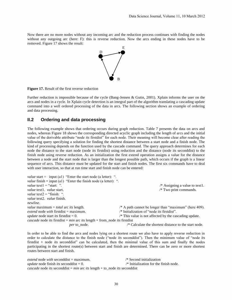
Now there are no more nodes without any incoming arc and the reduction process continues with finding the nodes

without any outgoing arc (here: F): this is reverse reduction. Now the arcs ending in these nodes have to be

removed. Figure 17 shows the result:

E

D

B

Figure 17. Result of the first reverse reduction

Further reduction is impossible because of the cycle (Bang-Jensen & Gutin, 2001). Xplain informs the user on the

arcs and nodes in a cycle. In Xplain cycle detection is an integral part of the algorithm translating a cascading update

command into a well ordered processing of the data in arcs. The following section shows an example of ordering

and data processing.

II.2 Ordering and data processing

The following example shows that ordering occurs during graph reduction. Table 7 presents the data on arcs and

nodes, whereas Figure 18 shows the corresponding directed acyclic graph including the length of arcs and the initial

value of the derivable attribute “node its firstdist” for each node. Their meaning will become clear after reading the

following query specifying a solution for finding the shortest distance between a start node and a finish node. The

kind of processing depends on the function used by the cascade command. The query approach determines for each

node the distance to the start node (node its firstdist) using reduction and the distance (node its seconddist) to the

finish node using reverse reduction. As an initialization the first extend operation assigns a value for the distance

between a node and the start node that is larger than the longest possible path, which occurs if the graph is a linear

sequence of arcs. This distance must be updated for the start and finish nodes. The first six commands have to deal

with user interaction, so that at run time start and finish node can be entered:

value start = input (a1) “Enter the start node (a letter): “.

value finish = input (a1) “Enter the finish node (a letter): “.

value text1 = “start: ”. /* Assigning a value to text1.

value text1. value start. /* Two print commands.

value text2 = “finish: “.

value text2. value finish.

newline.

value maximum = total arc its length. /* A path cannot be longer than “maximum” (here 409).

extend node with firstdist = maximum. /* Initialization of “node its firstdist”.

update node start its firstdist = 0. /* This value is not affected by the cascading update.

cascade node its firstdist = min arc its length + from_node its firstdist

per to_node. /* Calculate the shortest distance to the start node.

In order to be able to find the arcs and nodes lying on a shortest route we also have to apply reverse reduction in

order to calculate the distance to the finish node (“node its seconddist”). Then the minimum value of “node its

firstdist + node its seconddist” can be calculated, then the minimal value of this sum and finally the nodes

participating in the shortest route(s) between start and finish are determined. There can be zero or more shortest

routes between start and finish.

extend node with seconddist = maximum. /* Second initialization

update node finish its seconddist = 0. /* Initialization for the finish node.

cascade node its seconddist = min arc its length + to_node its seconddist


30

per from_node. /* Calculate the shortest distance to the finish node.

Now we can determine the nodes lying on a shortest route between start and finish:

extend node with distance = firstdist + seconddist. /* Distance to start + distance to finish.

value minimum = min node its distance. /* minimum: length of a shortest route.

extend node with OK = (distance = minimum and minimum < maximum). /* OK: node lies on a shortest route.

Because there can be more than one shortest route between two nodes it makes sense to include the relative position

of nodes to the position of the starting node:

value highest = count arc. /* If the graph is a sequence of arcs.

extend node with position = highest + 1. /* Initialization with the highest possible value.

update node start its position = 1. /* Initialization for the start node.

cascade node its position = min arc its from_node its position + 1

per to_node.

value comment1 = “The number of shortest routes from start to finish node is:”. value comment1.

get count arc where from_node its OK and to_node its OK and from_node = start.

newline.

value comment2 = “Nodes lying on a shortest route from start to finish node:”. value comment2.

newline.

value comment3 = “node id., position, firstdist, seconddist, distance”. value comment3.

get node its position, “ “, firstdist, “ “, seconddist, “ “, distance where OK

per firstdist. /* node identification is automatically included.

In the last retrieval the empty strings are included to create the desired presentation distance between the values to

be presented. The presentation order of nodes is by increasing value of the distance (per firstdist) to the start node.

If “B” is the start node and “K” the finish node then the query result is:

start:

B

finish:

K

The number of shortest routes from start to finish node is:

Count = 1

Nodes lying on a shortest route from start to finish node:

node id. position firstdist seconddist distance

B 1 0 102 102

D 2 18 84 102

F 3 39 63 102

G 4 63 39 102

H 5 83 19 102

K 6 102 0 102


31

If “K” is the start node and “B” the finish node then the result of the query is that there is not a shortest path KB:

start:

K

finish:

B


Count = 0



If “C” is the start node and “G” the finish node then the result of the query is:

start:

C

finish:

G


Count = 2



C 1 0 71 71

D 2 26 45 71

E 2 32 39 71

F 3 47 24 71

G 3 71 0 71

In the case of only one shortest route we can retrieve the nodes on that route in a well ordered manner: ordered by

the distance to the starting point. However, inherent in the described solution for the shortest path problem is that we

cannot specify the shortest routes separately if there is more than one shortest route. In the case of a shortest route

from “C” to “G” the user must be aware that there are two shortest routes and that arc EF is not part of a shortest

route because both “F” and “G” have the same relative position: 3. Each of these nodes lies on a different shortest

route from “C” to ”G”. Moreover, if CEFG would be a shortest route then the relative position of “G” must be one

higher than the relative position of “F”. Table 7 shows the data used for the construction of our example of an

acyclic directed graph.

Table 7. Data on arcs present in the graph of figure 18

arc from_node to_node length

1 A B 29

2 A C 22

3 C B 24

4 B D 18

5 C D 26

6 C E 32

7 D F 21

8 E F 26

9 E G 39

10 E K 61

11 E H 48

12 F G 24

13 G H 20

14 H K 19


32

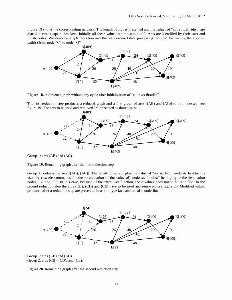
Figure 18 shows the corresponding network. The length of arcs is presented and the values of “node its firstdist” are

placed between square brackets. Initially all these values are the same: 409. Arcs are identified by their start and

finish nodes. We describe graph reduction and the well ordered data processing required for finding the shortest

path(s) from node “C” to node “G”.

B[409]

F[409]

D[409] 24 G[409] K[409]

29 18 21

24

A[409] 26 26 40 20 19

22 61

H[409]

C[0] 32 48

E[409]

Figure 18. A directed graph without any cycle after initialization of “node its firstdist”

The first reduction step produces a reduced graph and a first group of arcs [(AB) and (AC)] to be processed, see

figure 19. The arcs to be used and removed are presented as dotted arcs:

B[409]

F[409]

D[409] 24 G[409] K[409]

29 18 21

24

A[409] 26 26 40 20 19

22 61

H[409]

C[0] 32 48

E[409]

Group 1: arcs (AB) and (AC).

Figure 19. Remaining graph after the first reduction step

Group 1 contains the arcs [(AB), (AC)]. The length of an arc plus the value of “arc its from_node its firstdist” is

used by cascade commands for the recalculation of the value of “node its firstdist” belonging to the destination

nodes “B” and “C”. In this case, because of the “min” set function, these values need not to be modified. In the

second reduction step the arcs (CB), (CD) and (CE) have to be used and removed, see figure 20. Modified values

produced after a reduction step are presented in a bold type face and are also underlined.

B[24]

F[409]

D[26] 24 G[409] K[409]

29 18 21

24

A[409] 26 26 40 20 19

22 61

H[409]

C[0] 32 48

E[32]


Group 2: arcs (CB), (CD), and (CE).

Figure 20. Remaining graph after the second reduction step


33

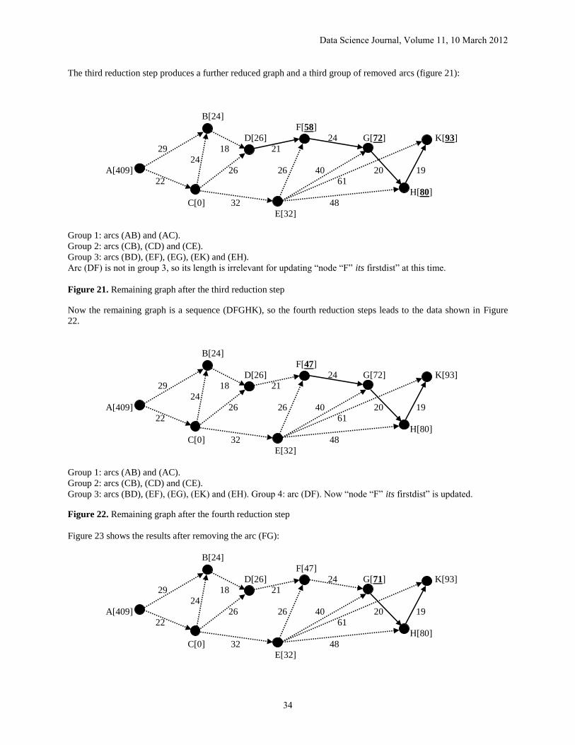
The third reduction step produces a further reduced graph and a third group of removed arcs (figure 21):

B[24]

F[58]

D[26] 24 G[72] K[93]

29 18 21

24

A[409] 26 26 40 20 19

22 61

H[80]

C[0] 32 48

E[32]


Group 2: arcs (CB), (CD) and (CE).

Group 3: arcs (BD), (EF), (EG), (EK) and (EH).

Arc (DF) is not in group 3, so its length is irrelevant for updating “node “F” its firstdist” at this time.

Figure 21. Remaining graph after the third reduction step

Now the remaining graph is a sequence (DFGHK), so the fourth reduction steps leads to the data shown in Figure

22.

B[24]

F[47]

D[26] 24 G[72] K[93]

29 18 21

24

A[409] 26 26 40 20 19

22 61

H[80]

C[0] 32 48

E[32]



Group 3: arcs (BD), (EF), (EG), (EK) and (EH). Group 4: arc (DF). Now “node “F” its firstdist” is updated.

Figure 22. Remaining graph after the fourth reduction step

Figure 23 shows the results after removing the arc (FG):

B[24]

F[47]

D[26] 24 G[71] K[93]

29 18 21

24

A[409] 26 26 40 20 19

22 61

H[80]

C[0] 32 48

E[32]


34

Group 1: the arcs (AB) and (AC).

Group 2: the arcs (CB), (CD) and (CE).

Group 3: the arcs (BD), (EF), (EG), (EK) and (EH). Group 4: arc (DF).

Group 5: arc (FG). Now “node “G” its firstdist” is updated.

Figure 23. Remaining graph after the fifth reduction step

In the sixth reduction step: arc (GH) has to be removed, see Figure 24 for the results:

B[24]

F[47]

D[26] 24 G[71] K[93]

29 18 21

24

A[409] 26 26 40 20 19

22 61

H[80]

C[0] 32 48

E[32]

Group 1: arcs 1(AB), 2(AC.

Group 2: arcs 3(CB), 5(CD), 6(CE).

Group 3: arcs 4(BD), 8(EF), 9(EG), 10(EK), 11(EH). Group 4: arc 7(DF).

Group 5: arc 12(FG). Group 6: arc 13(GH). Now “node “H” its firstdist” remains unchanged.

Figure 24. Remaining graph after the sixth reduction step

Figure 25 shows the results after the seventh reduction step, the removal of arc (HK):

B[24]

F[47]

D[26] 24 G[71] K[93]

29 18 21

24

A[409] 26 26 40 20 19

22 61

H[80]

C[0] 32 48

E[32]



Group 3: arcs (BD), (EF), (EG), (EK) and (EH).

Group 4: arc (DF).

Group 5: arc (FG).

Group 6: arc (GH).

Group 7: arc (HK). Now “node “K” its firstdist” remains the same.

Figure 25. Remaining graph after the seventh reduction step

Irrespective the kind of operation used by a cascade command the properties (intrinsic or derived) of the arcs are

used in the following order: group 1, group 2, group 3, group 4, group 5, group 6, group 7. Within each group the

processing order is irrelevant.

In a similar way the reverse graph reduction is executed for the calculation of “node its seconddist”. Further

processing and presenting the results has been described in the query.


35

(Article history: Received 11 March 2010, Accepted 9 February 2012, Available online 17 February 2012)


36

IMPROVING DATA QUALITY CONTROL IN THE XPLAIN-DBMS

Documents

Transcript of IMPROVING DATA QUALITY CONTROL IN THE XPLAIN-DBMS