Improving abdomen tumor low-dose CT images using a

fast dictionary learning based processing.

Yang Chen, Xindao Yin, Luyao Shi, Huazhong Shu, Limin Luo, Jean-Louis

Coatrieux, Christine Toumoulin

To cite this version:

Yang Chen, Xindao Yin, Luyao Shi, Huazhong Shu, Limin Luo, et al.. Improving abdomen tu-mor low-dose CT images using a fast dictionary learning based processing.. Physics in Medicineand Biology, IOP Publishing, 2013, 58 (16), pp.5803-20. <10.1088/0031-9155/58/16/5803>.<inserm-00874944>

HAL Id: inserm-00874944

http://www.hal.inserm.fr/inserm-00874944

Submitted on 12 Aug 2014

HAL is a multi-disciplinary open accessarchive for the deposit and dissemination of sci-entific research documents, whether they are pub-lished or not. The documents may come fromteaching and research institutions in France orabroad, or from public or private research centers.

L’archive ouverte pluridisciplinaire HAL, estdestinee au depot et a la diffusion de documentsscientifiques de niveau recherche, publies ou non,emanant des etablissements d’enseignement et derecherche francais ou etrangers, des laboratoirespublics ou prives.

> REPLACE THIS LINE WITH YOUR PAPER IDENTIFICATION NUMBER (DOUBLE-CLICK HERE TO EDIT) <

1

Yang Chen1,2,3,4, Xindao Yin5, Luyao Shi1,2, Huazhong Shu1,2, Limin Luo1,2, Jean-Louis Coatrieux1,2,3,4 and Christine Toumoulin2,3,4 1. Laboratory of Image Science and Technology, Southeast University, 210096, Nanjing, People’s Republic of China 2. Centre de Recherche en Information Biomedicale Sino-Francais (LIA CRIBs), Rennes, France 3. Laboratoire Traitement du Signal et de l’Image (LTSI), Université de Rennes 1, F-35042 Rennes, France 4. INSERM, U1099, F-35042, Rennes, France 5. Department of Radiology, Nanjing Hospital Affiliated to Nanjing Medical University, 210096, People’s Republic of China

Abstract—In abdomen computed tomography (CT), repeated radiation exposures are often inevitable for cancer patients who receive guided surgery or radiotherapy. Low-dose scans should thus be considered in order to avoid too high accumulative harm of radiation. This work is aimed at improving abdomen tumor CT images from low-dose scans by using a fast dictionary learning (DL) based processing. Stemming from sparse representation theory, the patch-based DL approach proposed in this paper allows effective suppression of both mottled noise and streak artifacts. The experiments carried out on clinical data show that the proposed method brings encouraging improvements in abdomen low-dose CT images with tumors.

Keywords—Low-dose CT (LDCT), abdomen tumor, dictionary learning, noise, artifacts

1.Introduction

Since the introduction of computed tomography (CT) in the 1970s, a wide-spread concern on CT is the increasing risk of cancer induced by X-ray radiation [1-2]. The radiation doses delivered to patients during X-ray CT examinations are relatively high when compared to other radiological examinations [3]. Based on a recent report, the overall averaged radiation dose associated with a routine abdomen/pelvis CT scan is around 10 mSv, which is roughly 5 times of head CTs and 100 times of chest X-ray Radiography [3]. Additionally, the dose in CT is cumulative in lifetime, and successive CT scanning can significantly increase the lifetime radiation risk of fatal cancers [3-4].

CT is also frequently used to guide the surgery or radiotherapy by providing localized contrast information between tumors, organs and other surrounding human tissues. Patients with diagnosed or suspicious abdomen tumors would be submitted to repeated CT scans over a long observing period before or after surgery or therapy. Low dose CT (LDCT) is therefore of major importance in order to alleviate the harm

caused by cumulated radiations for the patients with abdomen tumors. Among all the methods proposed so far to obtain LDCT images, the most practical and widely used method is lowering the X-ray tube current by modulating the mA or mAs setting, but at a cost of degraded CT image quality due to increased quantum noise and artifacts [5-7]. In the past ten years, other approaches have been explored to improve the quality of LDCT images. They can be divided into three categories: pre-processing approaches, reconstruction approaches and post-processing approaches.

The first one refers to techniques that improve the CT imaging by restoring the projected raw data before filtered-backprojection (FBP) reconstruction. Adaptive filtering, multiscale penalized weighted least-squares and bilateral filtering have been reported to suppress the excessive quantum noise in projected raw data [8-10]. Reconstruction approaches treat the LDCT imaging as an ill-posed inverse problem, and solve the problem via maximizing a prior-regularized cost function using iterative optimizations [11-19]. Many prior options have been proposed in the past decade, for example the total-variation minimization in [14], the nonlocal prior reconstruction in [15-16], and the prior image constrained compressed sensing (PICCS) algorithm in [17]. It

Improving Abdomen Tumor Low-dose CT Images Using A Fast Dictionary Learning Based Processing

> REPLACE THIS LINE WITH YOUR PAPER IDENTIFICATION NUMBER (DOUBLE-CLICK HERE TO EDIT) <

2

should be noted that results of clinical value in abdomen LDCT have been achieved by using the PICCS algorithm [17] and the adaptive statistical iterative reconstruction (ASIR) [18-19]. However, due to the difficult access to well-formatted projection data of the main CT vendors, researches on pre-processing and reconstruction approaches are often limited in practice. Another well-known concern for iterative reconstructions is the intensive computation cost required for reconstruction, which may delay clinical workflow and diagnosis. Additionally, the CT scanners equipped in most current hospitals are based on FBP algorithms and upgrading to the latest CT scanners with iterative algorithm is often too expensive.

The approach described in this paper falls into the third category, i.e post-processing methods. They can be directly applied on LDCT images to suppress noise and artifacts. The main merits of post-processing methods include their low computation cost and their easy implementation in most current CT systems with no built-in low dose solutions. The objective when applying post-processing on LDCT images is to obtain images with visual appearances close to the corresponding SDCT (standard dose CT) images without introducing structure lost and new artifacts (or false structures). However, due to the fact that the back-projection process in the FBP algorithm distributes the noise and artifacts non-uniformly over the whole image, CT noise and artifacts with mottled or streak effects are often difficult to be removed from already reconstructed images. The noise and artifacts in abdomen LDCT images cannot be modeled by Gaussian or Poisson distributions and restorations based on such priors lead to poor performance. This explains why post-processing techniques rely on more heuristic approaches. Furthermore, compared to other abdominal pathological features such as hepatic cyst, tumor tissues are often of lower contrast, and it is rather challenging to preserve their characteristics through image processing [7]. In [20-21], several noise reduction filters were proposed to enhance the conspicuity of lesions in abdomen LDCT images. An adaptive noise reduction filtering which combines smoothing and edge-enhancing was reported to gain 50% dose reduction (tube current reduced from 160mAs to 80mAs) without losing low-contrast detectability [22]. In [23], a filtering technique, named large-scale nonlocal means (LNLM), was proposed to improve the quality of abdomen LDCT images with hepatic cysts. This LNLM method was further combined with a multiscale directional diffusion to suppress the streak artifacts in thoracic CT images [24].

Recent years have witnessed a growing interest in the study of sparse and redundant representations over dictionary learning (DL) [25-32]. Some successful applications have been explored in medical imaging [33-35]. Instead of being based on a pixel-wise intensity update, patch-wise DL processing inherently enables a more effective representation of patch-shaped features such as tumors or organs. In the paper, we propose to apply patch-based DL processing to improve abdomen tumor LDCT images. This method is referred to as DL algorithm. In the experiments presented below, clinical LDCT images of cancer patients were used. The corresponding SDCT images were also acquired to have a ground truth reference. The

proposed DL algorithm can be efficiently implemented by using a global dictionary and a parallelization technique. The relevance of this DL approach is shown through experiments conducted on a large set of patients. The structure of this paper is as follows: in Section 2, the acquisition protocol, the patient set and the proposed algorithm are described. Results are given and discussed in Section 3. Section 4 concludes this paper with a brief description of its contributions and some open questions for future work.

2. Material and methods 2.1. Clinical data and processing environment

The protocol of this study (data collection and post-processing) was approved by our institutional ethical review board. 25 patients were involved in the experiments. All these patients have given their written consent to the participation and received remuneration for it. A non-conflict of interest for this work was declared. CT images were acquired on a multi-detector row Siemens Somatom Sensation 16 CT scanner.

The patient cohort includes 11 women and 14 men with an average age of 64 years (age range: 54-73 years). All the patients suffer from cancers confirmed by biopsy examinations. Both LDCT and SDCT images were collected using a reduced tube current 50mAs and the routine tube current 260mAs under abdomen scan mode. 40 slices were collected for each patient scan. Other scan parameters include: kVp, 120; slice thickness, 5 mm; Gantry rotation time, 0.5s; detector configuration (detector rows section thickness), 16 mm 1.5 mm; table feed per gantry rotation, 24 mm; pitch, 1:1; reconstruction method: FBP algorithm with convolution kernel “B20f” (“B20f” is the routine smoothing kernel used in reconstructing abdomen images on Siemens CT). Here we consider the abdomen window (center, 50HU; width, 350HU). The volume CT dose index (CTDIvol) is a linear function of the tube currents [6]. We recorded the accumulated doses from the workstation for each scan with 40 slices. The recorded doses are 16.38 mGy for the routine 260 mAs protocol, and 3.09 mGy for the low dose 50 mAs protocol. All the CT images were exported as DICOM files and then processed offline under a PC workstation (Intel Core™ 2 Quad CPU and 4096 Mb RAM, GPU (NVIDIA GTX465)) with Visual C++ as the developing language (Visual Studio 2008 software; Microsoft).

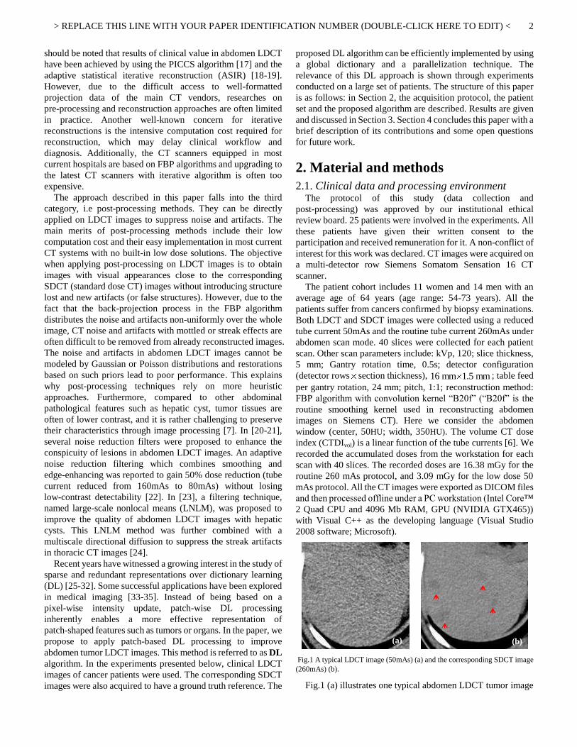
Fig.1 A typical LDCT image (50mAs) (a) and the corresponding SDCT image (260mAs) (b).

Fig.1 (a) illustrates one typical abdomen LDCT tumor image

(a)

(b)

> REPLACE THIS LINE WITH YOUR PAPER IDENTIFICATION NUMBER (DOUBLE-CLICK HERE TO EDIT) <

3

with multiple hepatic metastases and Fig.1 (b) is the corresponding SDCT image for reference. The LDCT image and SDCT image were respectively acquired with 50mAs and 260mAs, as specified above, and other scanning parameters were both kept as routine setting. We can see that (i) the LDCT image is significantly degraded by mottled noise with strong intensity variation and (ii) the patch-shaped tumor tissues (pointed by arrows) present a low contrast with the surrounding tissues. Therefore, processing LDCT tumor images in abdomen scans should be targeted at improving LDCT image quality and obtaining an enhanced detectability of abdomen tumors.

2.2. Method and parameter setting

The proposed DL-based patch processing was performed on 2-D slices because of the large slice thickness setting in routine abdomen CT scanning (>=1mm, 5mm in this work).

Assuming the patches in the target LDCT images are sparsely representable, DL-based patch processing can be carried out by coding each patch as a linear combination of only a few patches in the dictionary [26-27]. This method finds the best global over-complete dictionary and represents each image patch as a linear combination of only a few dictionary vectors (atoms). The coefficients of the linear combination are estimated through a sparse coding process [28]. Based on [29] and [35], the DL-based patch processing aims at solving the following problem:

22

2 2 0, ,

min s.t. , ij ij ij

Dij

xR D i jx y x T (1)

where, x and y denote the processed and the original LDCT images respectively, and the subscript ij denotes the pixel index

(i, j) in the image. ijR represents the operator that extracts the

patch ijx of size n n (centered at (i, j)) from image x. The

patch-based dictionary D is a n K matrix, which is composed of K n-vector atoms (columns). Each n-vector column corresponds to one n n patch. denotes the coefficient set

ij ij for all the sparse representations of patches, and each

patch ijx can be approximated by a linear combination ijD .

0|| ||

ij denotes the 0l norm that counts the nonzero entries of

vector ij , and T is the preset parameter of sparsity level that

limits the maximum nonzero entry number in ij . Based on [29],

solving (1) includes the following two steps (2) and (3): 2

2 0,

min s.t. , ij ij ij

Dij

R D i jx T (2)

22

2 2min

ij ij

ijx

R Dx y x (3)

The objective of Eq. (2) is to train the coefficients and dictionary D from a set of image patches. It can be efficiently solved by k-means singular value decomposition (K-SVD) with the replacement of x by the known observed image y [29]. Starting from an initial dictionary (e.g. the Discrete Cosine Transform dictionary, DCT dictionary), this K-SVD operation estimates and D by alternatively applying the orthogonal

marching pursuit (OMP) algorithm and the SVD decomposition [29]. The columns of the dictionary D are constrained to be of unit norm to avoid scaling ambiguity in practical calculation [35]. Then, when dictionary D and are obtained, we can obtain the output image x by solving the first order derivative of (3) with respect to each pixel in x:

1

ij

ij ijij ij ij

T TR R Rx I y D (4)

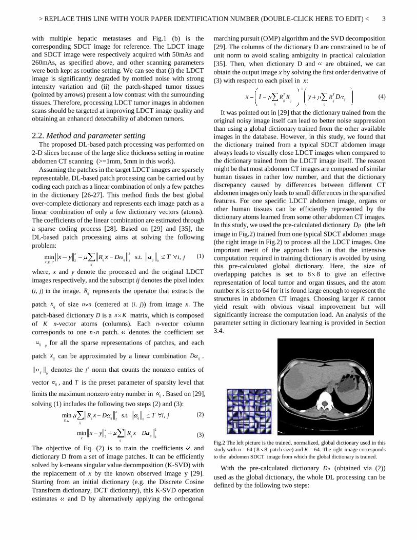
It was pointed out in [29] that the dictionary trained from the original noisy image itself can lead to better noise suppression than using a global dictionary trained from the other available images in the database. However, in this study, we found that the dictionary trained from a typical SDCT abdomen image always leads to visually close LDCT images when compared to the dictionary trained from the LDCT image itself. The reason might be that most abdomen CT images are composed of similar human tissues in rather low number, and that the dictionary discrepancy caused by differences between different CT abdomen images only leads to small differences in the sparsified features. For one specific LDCT abdomen image, organs or other human tissues can be efficiently represented by the dictionary atoms learned from some other abdomen CT images. In this study, we used the pre-calculated dictionary pD (the left image in Fig.2) trained from one typical SDCT abdomen image (the right image in Fig.2) to process all the LDCT images. One important merit of the approach lies in that the intensive computation required in training dictionary is avoided by using this pre-calculated global dictionary. Here, the size of overlapping patches is set to 8 8 to give an effective representation of local tumor and organ tissues, and the atom number K is set to 64 for it is found large enough to represent the structures in abdomen CT images. Choosing larger K cannot yield result with obvious visual improvement but will significantly increase the computation load. An analysis of the parameter setting in dictionary learning is provided in Section 3.4.

Fig.2 The left picture is the trained, normalized, global dictionary used in this study with n = 64 (8 8 patch size) and K = 64. The right image corresponds to the abdomen SDCT image from which the global dictionary is trained.

With the pre-calculated dictionary pD (obtained via (2)) used as the global dictionary, the whole DL processing can be defined by the following two steps:

> REPLACE THIS LINE WITH YOUR PAPER IDENTIFICATION NUMBER (DOUBLE-CLICK HERE TO EDIT) <

4

2

20(S1), min s.t. ,

ij ij ij

ij

pR x i jD (5)

22

2 2(S2), min

ij ij

ijx

pRx y x D (6)

Here, the sparse coefficient set and the image x can be calculated by solving (5) and (6) using OMP and the solution given in (4). In (5), denotes the tolerance parameter used in calculating by OMP method.

For evaluation purpose, we compared the proposed method with the LNLM method, which is a pixel-wise weighted intensity summation with weights determined by patch similarities [23]. The intensive pixel-wise operations in LNLM method was accelerated using GPU (Graphics Processing Unit) techniques based on [23]. The parameters involved in the LNLM and proposed DL methods were specified under the guidance of one radiological doctor (X.D.Y. with 15 years of experience) to provide the best visual results. Practically, we found that the same parameter setting can be used to process the LDCT images with the same scan protocol for the two methods. TABLE I lists this parameter setting. For the LNLM method, the parameter h, the patch size Np and the neighborhood size Nn were set to 2, 7 7 and 81 81, respectively. For the proposed DL method, as shown in Fig. 3, the dictionary size was set to 64 64 for 8 8 patch (n = 64) and 64 atom numbers (K = 64). Sparsity level

0L was set to 3 atoms, and 20 iterations (Itern=20)

were used in the K-SVD calculation to update the dictionary D and the sparse coefficient . The initial dictionary for K-SVD is the DCT dictionary obtained by sampling the cosine wave functions in different frequencies. The tolerance parameter and in (5) and (6) were set to 21 and 0.8.

TABLE I THE PARAMETER SETTINGS AND COMPUTATION COST (IN SECOND) FOR THE

LNLM METHOD IN [23] AND THE PROPOSED METHOD

LNLM method DL method

Parameter settings

h =4, =7 7pN ,

=81 81nN

K = 64, n = 8, =3T , Itern=20,

=21, =0.8

3. Results 3.1. Visual assessment

Here, the complete images are displayed using the standard abdomen window and in full size in order to facilitate an overall quality evaluation. Fig.2 shows the trained dictionaries (D) used in the implementation of the proposed DL method.

The low dose CT data in Fig.3-Fig.5 are respectively from a 61 years female patient, a 53 years female patient, and a 56

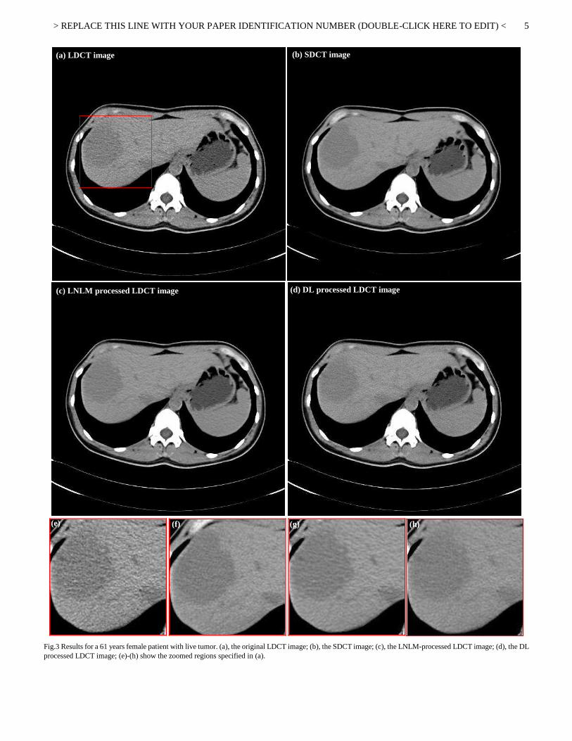
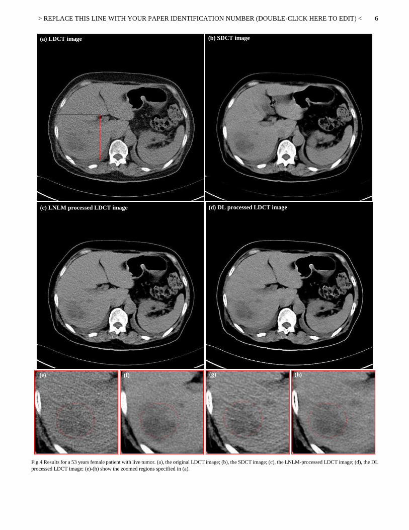
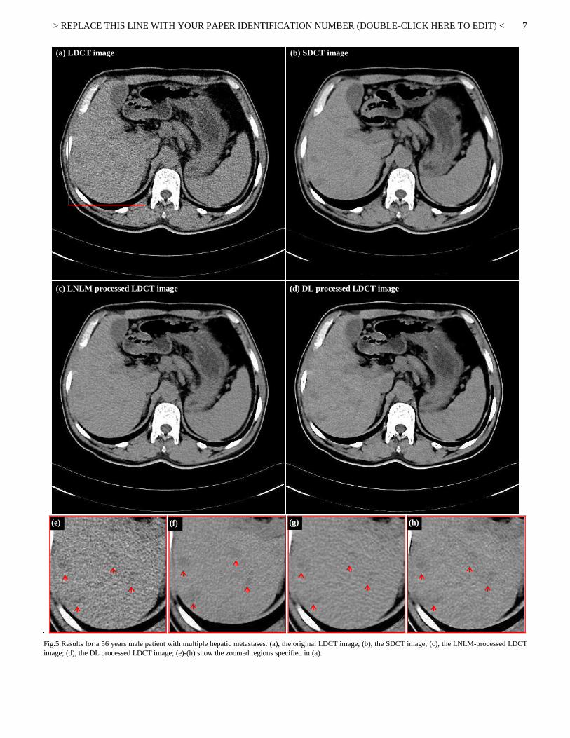
years male patient. To be more precise, Fig.3(a) and Fig.4(a) are respectively two LDCT images with live tumors, and Fig.5(a) is a LDCT image with hepatic metastases. (b) and (d) in Fig.3-Fig.5 show the corresponding SDCT images and the DL processed LDCT images. Fig.3(c), Fig.4(c) and Fig.5(c) show the LNLM processed images. In Fig.3-Fig.5, (e)-(h) illustrate the zoomed regions of interest (ROI) identified by squares in (a). We should note here that, for the SDCT images, the ROIs with the closest visual match with the LDCT images are selected because of the unavoidable displacements between the two different scans. From all (a) in Fig.3-Fig.5, we observe that, under low dose CT scanning condition, mottled noise and streak artifacts severely degrade the image quality and lead to unclear tumor boundaries. With the SDCT images as reference, we can see in (c) in Fig.3-Fig.5 that the LNLM method can suppress noise and artifacts but tends to introduce some strange striped artifacts and so leads to lowered perceptive detectability of small lesions (arrows in Fig.5(g)). In particular, referring to the case of multiple hepatic metastases in Fig.5, we can note that the proposed DL processed image allows a better discrimination of small lesions (arrows in Fig.5(h)) when compared to the original LDCT image and the LNLM processed image.

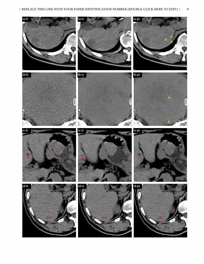
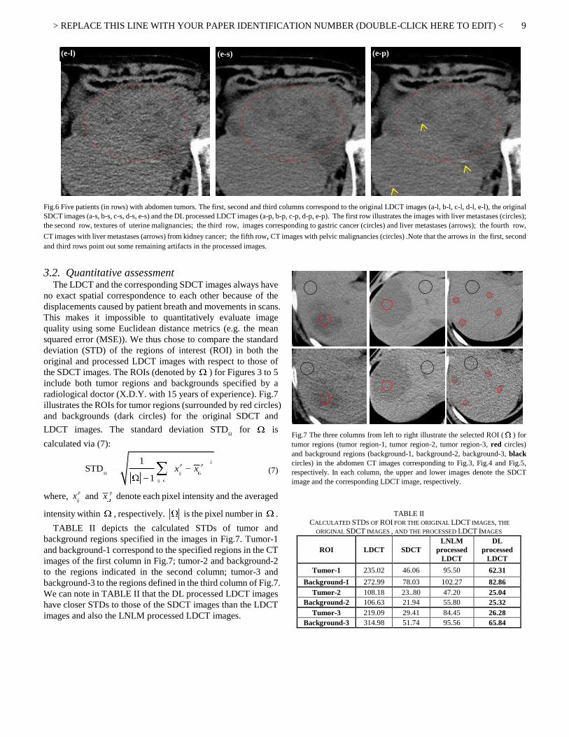
Fig.6 provides the processing results of another five patients with abdomen tumors. The first, second and third columns correspond to the original LDCT images (a-l, b-l, c-l, d-l, e-l), the original SDCT images (a-s, b-s, c-s, d-s, e-s) and the DL processed LDCT images (a-p, b-p, c-p, d-p, e-p). To be specific, in Fig.6, the first row depicts images with liver metastases (a-l, a-s, a-p); the second row displays images of uterine malignancies (b-l, b-s, b-p); the third row illustrates images with gastric cancer and liver metastases (c-l, c-s, c-p); the fourth row shows images with kidney cancer and liver metastases (d-l, d-s, d-p); the fifth row, images with pelvic malignancies (e-l, e-s, e-p) are given. We can clearly see that a significant improvement of image quality can be obtained by processing the original LDCT images using the proposed DL algorithm. In the processed LDCT images, both noise and artifacts are effectively suppressed, which leads to better visibility of tumor tissues.

By comparing the processed LDCT images with the original SDCT images in Fig.3-Fig.6, we can observe that the proposed DL method can produce LDCT image with textures visually closer to those of the original SDCT images. However, in the DL processed LDCT images we can still notice that some original high contrast artifacts still remain (see arrows in Fig.6 a-p, b-p and e-p). The DL algorithm might be not effective in suppressing such high contrast singular artifacts.

> REPLACE THIS LINE WITH YOUR PAPER IDENTIFICATION NUMBER (DOUBLE-CLICK HERE TO EDIT) <

5

Fig.3 Results for a 61 years female patient with live tumor. (a), the original LDCT image; (b), the SDCT image; (c), the LNLM-processed LDCT image; (d), the DL processed LDCT image; (e)-(h) show the zoomed regions specified in (a).

(a) LDCT image

(d) DL processed LDCT image

(e)

(h)

(b) SDCT image

(f)

(c) LNLM processed LDCT image

(g)

> REPLACE THIS LINE WITH YOUR PAPER IDENTIFICATION NUMBER (DOUBLE-CLICK HERE TO EDIT) <

6

Fig.4 Results for a 53 years female patient with live tumor. (a), the original LDCT image; (b), the SDCT image; (c), the LNLM-processed LDCT image; (d), the DL processed LDCT image; (e)-(h) show the zoomed regions specified in (a).

(e)

(f)

(h)

(a) LDCT image

(b) SDCT image

(g)

(c) LNLM processed LDCT image

(d) DL processed LDCT image

> REPLACE THIS LINE WITH YOUR PAPER IDENTIFICATION NUMBER (DOUBLE-CLICK HERE TO EDIT) <

7

Fig.5 Results for a 56 years male patient with multiple hepatic metastases. (a), the original LDCT image; (b), the SDCT image; (c), the LNLM-processed LDCT image; (d), the DL processed LDCT image; (e)-(h) show the zoomed regions specified in (a).

(a) LDCT image

(b) SDCT image

(h)

(d) DL processed LDCT image

(c) LNLM processed LDCT image

(g)

(f)

(e)

> REPLACE THIS LINE WITH YOUR PAPER IDENTIFICATION NUMBER (DOUBLE-CLICK HERE TO EDIT) <

8

(a-l)

(a-s)

(a-p)

(b-l)

(b-s)

(b-p)

(c-l)

(c-s)

(c-p)

(d-l)

(d-s)

(d-p)

> REPLACE THIS LINE WITH YOUR PAPER IDENTIFICATION NUMBER (DOUBLE-CLICK HERE TO EDIT) <

9

Fig.6 Five patients (in rows) with abdomen tumors. The first, second and third columns correspond to the original LDCT images (a-l, b-l, c-l, d-l, e-l), the original SDCT images (a-s, b-s, c-s, d-s, e-s) and the DL processed LDCT images (a-p, b-p, c-p, d-p, e-p). The first row illustrates the images with liver metastases (circles); the second row, textures of uterine malignancies; the third row, images corresponding to gastric cancer (circles) and liver metastases (arrows); the fourth row,

CT images with liver metastases (arrows) from kidney cancer; the fifth row, CT images with pelvic malignancies (circles) .Note that the arrows in the first, second and third rows point out some remaining artifacts in the processed images.

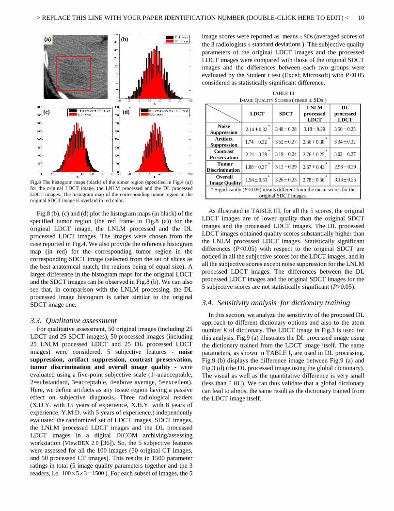
3.2. Quantitative assessment The LDCT and the corresponding SDCT images always have

no exact spatial correspondence to each other because of the displacements caused by patient breath and movements in scans. This makes it impossible to quantitatively evaluate image quality using some Euclidean distance metrics (e.g. the mean squared error (MSE)). We thus chose to compare the standard deviation (STD) of the regions of interest (ROI) in both the original and processed LDCT images with respect to those of the SDCT images. The ROIs (denoted by ) for Figures 3 to 5 include both tumor regions and backgrounds specified by a radiological doctor (X.D.Y. with 15 years of experience). Fig.7 illustrates the ROIs for tumor regions (surrounded by red circles) and backgrounds (dark circles) for the original SDCT and

LDCT images. The standard deviation ΩSTD for is

calculated via (7):

2

Ω

1STD

1

p p

ij

ij

x x

(7)

where, p

ijx and px denote each pixel intensity and the averaged

intensity within , respectively. is the pixel number in .

TABLE II depicts the calculated STDs of tumor and background regions specified in the images in Fig.7. Tumor-1 and background-1 correspond to the specified regions in the CT images of the first column in Fig.7; tumor-2 and background-2 to the regions indicated in the second column; tumor-3 and background-3 to the regions defined in the third column of Fig.7. We can note in TABLE II that the DL processed LDCT images have closer STDs to those of the SDCT images than the LDCT images and also the LNLM processed LDCT images.

Fig.7 The three columns from left to right illustrate the selected ROI ( ) for tumor regions (tumor region-1, tumor region-2, tumor region-3, red circles) and background regions (background-1, background-2, background-3, black circles) in the abdomen CT images corresponding to Fig.3, Fig.4 and Fig.5, respectively. In each column, the upper and lower images denote the SDCT image and the corresponding LDCT image, respectively.

TABLE II CALCULATED STDS OF ROI FOR THE ORIGINAL LDCT IMAGES, THE

ORIGINAL SDCT IMAGES , AND THE PROCESSED LDCT IMAGES

ROI LDCT SDCT LNLM

processed LDCT

DL processed

LDCT

Tumor-1 235.02 46.06 95.50 62.31

Background-1 272.99 78.03 102.27 82.86 Tumor-2 108.18 23..80 47.20 25.04

Background-2 106.63 21.94 55.80 25.32 Tumor-3 219.09 29.41 84.45 26.28

Background-3 314.98 51.74 95.56 65.84

(e-l)

(e-s)

(e-p)

> REPLACE THIS LINE WITH YOUR PAPER IDENTIFICATION NUMBER (DOUBLE-CLICK HERE TO EDIT) <

10

Fig.8 The histogram maps (black) of the tumor region (specified in Fig.4 (a)) for the original LDCT image, the LNLM processed and the DL processed LDCT images. The histogram map of the corresponding tumor region in the original SDCT image is overlaid in red color.

Fig.8 (b), (c) and (d) plot the histogram maps (in black) of the specified tumor region (the red frame in Fig.8 (a)) for the original LDCT image, the LNLM processed and the DL processed LDCT images. The images were chosen from the case reported in Fig.4. We also provide the reference histogram map (in red) for the corresponding tumor region in the corresponding SDCT image (selected from the set of slices as the best anatomical match, the regions being of equal size). A larger difference in the histogram maps for the original LDCT and the SDCT images can be observed in Fig.8 (b). We can also see that, in comparison with the LNLM processing, the DL processed image histogram is rather similar to the original SDCT image one.

3.3. Qualitative assessment

For qualitative assessment, 50 original images (including 25 LDCT and 25 SDCT images), 50 processed images (including 25 LNLM processed LDCT and 25 DL processed LDCT images) were considered. 5 subjective features - noise suppression, artifact suppression, contrast preservation, tumor discrimination and overall image quality - were evaluated using a five-point subjective scale (1=unacceptable, 2=substandard, 3=acceptable, 4=above average, 5=excellent). Here, we define artifacts as any tissue region having a passive effect on subjective diagnosis. Three radiological readers (X.D.Y. with 15 years of experience, X.H.Y. with 8 years of experience, Y.M.D. with 5 years of experience.) independently evaluated the randomized set of LDCT images, SDCT images, the LNLM processed LDCT images and the DL processed LDCT images in a digital DICOM archiving/assessing workstation (ViewDEX 2.0 [36]). So, the 5 subjective features were assessed for all the 100 images (50 original CT images, and 50 processed CT images). This results in 1500 parameter ratings in total (5 image quality parameters together and the 3 readers, i.e. 100 5 3 1500). For each subset of images, the 5

image scores were reported as SDsmeans (averaged scores of the 3 radiologists± standard deviations). The subjective quality parameters of the original LDCT images and the processed LDCT images were compared with those of the original SDCT images and the differences between each two groups were evaluated by the Student t test (Excel; Microsoft) with P<0.05 considered as statistically significant difference.

TABLE III IMAGE QUALITY SCORES ( mean SDs± )

LDCT SDCT LNLM

processed LDCT

DL processed

LDCT Noise

Suppression 2.14 0.32

* 3.48 0.28 3.18 0.29 3.50 0.25

Artifact Suppression

1.74 0.32* 3.52 0.27 2.36 0.38

* 3.34 0.32

Contrast Preservation

2.21 0.28* 3.19 0.24 2.76 0.25

* 3.02 0.27

Tumor Discrimination

1.88 0.37* 3.12 0.29 2.67 0.43

* 2.98 0.29

Overall Image Quality

1.94 0.33* 3.26 0.23 2.78 0.36

* 3.13 0.25

* Significantly (P<0.05) means different from the mean scores for the original SDCT images.

As illustrated in TABLE III, for all the 5 scores, the original

LDCT images are of lower quality than the original SDCT images and the processed LDCT images. The DL processed LDCT images obtained quality scores substantially higher than the LNLM processed LDCT images. Statistically significant differences (P<0.05) with respect to the original SDCT are noticed in all the subjective scores for the LDCT images, and in all the subjective scores except noise suppression for the LNLM processed LDCT images. The differences between the DL processed LDCT images and the original SDCT images for the 5 subjective scores are not statistically significant (P>0.05).

3.4. Sensitivity analysis for dictionary training

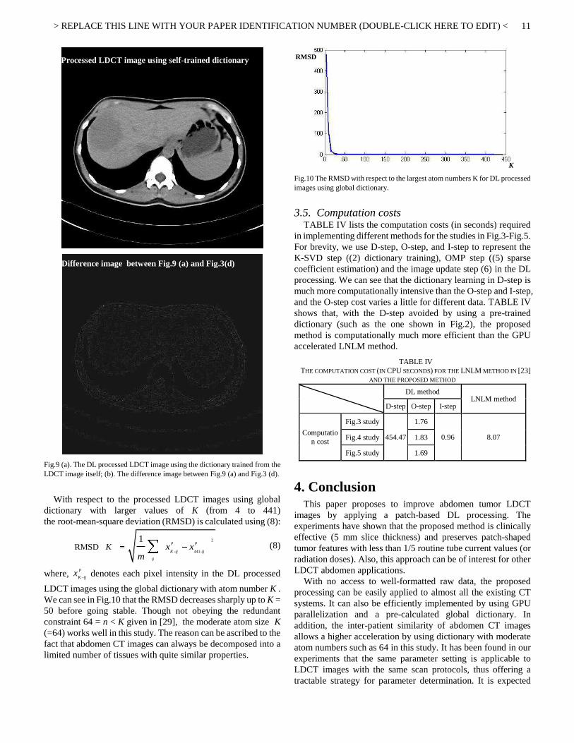
In this section, we analyze the sensitivity of the proposed DL approach to different dictionary options and also to the atom number K of dictionary. The LDCT image in Fig.3 is used for this analysis. Fig.9 (a) illustrates the DL processed image using the dictionary trained from the LDCT image itself. The same parameters, as shown in TABLE I, are used in DL processing. Fig.9 (b) displays the difference image between Fig.9 (a) and Fig.3 (d) (the DL processed image using the global dictionary). The visual as well as the quantitative difference is very small (less than 5 HU). We can thus validate that a global dictionary can lead to almost the same result as the dictionary trained from the LDCT image itself.

(a)

(b)

(c)

(d)

> REPLACE THIS LINE WITH YOUR PAPER IDENTIFICATION NUMBER (DOUBLE-CLICK HERE TO EDIT) <

11

Fig.9 (a). The DL processed LDCT image using the dictionary trained from the LDCT image itself; (b). The difference image between Fig.9 (a) and Fig.3 (d).

With respect to the processed LDCT images using global dictionary with larger values of K (from 4 to 441) the root-mean-square deviation (RMSD) is calculated using (8):

2

- 441-RMSD

1p p

K ij ij

ij

K x xm

(8)

where, -

p

K ijx denotes each pixel intensity in the DL processed

LDCT images using the global dictionary with atom number K . We can see in Fig.10 that the RMSD decreases sharply up to K = 50 before going stable. Though not obeying the redundant constraint 64 = n < K given in [29], the moderate atom size K (=64) works well in this study. The reason can be ascribed to the fact that abdomen CT images can always be decomposed into a limited number of tissues with quite similar properties.

Fig.10 The RMSD with respect to the largest atom numbers K for DL processed images using global dictionary.

3.5. Computation costs

TABLE IV lists the computation costs (in seconds) required in implementing different methods for the studies in Fig.3-Fig.5. For brevity, we use D-step, O-step, and I-step to represent the K-SVD step ((2) dictionary training), OMP step ((5) sparse coefficient estimation) and the image update step (6) in the DL processing. We can see that the dictionary learning in D-step is much more computationally intensive than the O-step and I-step, and the O-step cost varies a little for different data. TABLE IV shows that, with the D-step avoided by using a pre-trained dictionary (such as the one shown in Fig.2), the proposed method is computationally much more efficient than the GPU accelerated LNLM method.

TABLE IV THE COMPUTATION COST (IN CPU SECONDS) FOR THE LNLM METHOD IN [23]

AND THE PROPOSED METHOD

DL method

LNLM method D-step O-step I-step

Computation cost

Fig.3 study

454.47

1.76

0.96 8.07 Fig.4 study 1.83

Fig.5 study 1.69

4. Conclusion This paper proposes to improve abdomen tumor LDCT

images by applying a patch-based DL processing. The experiments have shown that the proposed method is clinically effective (5 mm slice thickness) and preserves patch-shaped tumor features with less than 1/5 routine tube current values (or radiation doses). Also, this approach can be of interest for other LDCT abdomen applications.

With no access to well-formatted raw data, the proposed processing can be easily applied to almost all the existing CT systems. It can also be efficiently implemented by using GPU parallelization and a pre-calculated global dictionary. In addition, the inter-patient similarity of abdomen CT images allows a higher acceleration by using dictionary with moderate atom numbers such as 64 in this study. It has been found in our experiments that the same parameter setting is applicable to LDCT images with the same scan protocols, thus offering a tractable strategy for parameter determination. It is expected

(a) Processed LDCT image using self-trained dictionary

(b) Difference image between Fig.9 (a) and Fig.3(d)

RMSDSD

KS

> REPLACE THIS LINE WITH YOUR PAPER IDENTIFICATION NUMBER (DOUBLE-CLICK HERE TO EDIT) <

12

that the proposed DL approach can also be well used in the processing of other LDCT abdomen data.

Nonetheless, we also found that some artifacts with strong contrast were hard to be suppressed without blurring tumor structures. This effect is expected to be more severe in the case of thinner slices. The reason might be that only limited similarity information within a small neighboring region is used in the proposed DL algorithm. Also, the whole computation cost of the DL processing still needs a further acceleration to fulfill practical clinical requirements (less than 0.5 second per 2-D slice). Currently, some parameters (e.g. the sparsity level and tolerance parameter) still need to be empirically set. Future work will thus be devoted to improvements by incorporating some artifact-suppressing constraints trained from available SDCT images, extending the application to 3D in order to deal with cases with thin slice thicknesses, further accelerating the OMP computation in DL processing by using parallelization techniques, and also developing more robust estimation for parameters.

Acknowledgments This research was supported by National Basic Research

Program of China under grant (2010CB732503), National Natural Science Foundation under grants (81000636), and the Project supported by Natural Science Foundations of Jiangsu Province (BK2011593).

References [1] A. C. Kak and M. Slaney, Principles of Computerized Tomographic Imaging.

Philadelphia, PA: SIAM, 2001. [2] D. J. Brenner and E. J. Hall, "Computed tomography-an increasing source of

radiation exposure," New England Journal of Medicine, Vol.357, pp. 2277-2284, 2007.

[3] Patient safety: Radiation Exposure in X-ray and CT Examinations, http://www.radiologyinfo.org/en/safety/index.cfm?pg=sfty_xray.

[4] Smith-Bindman R, Lipson J, Marcus R, Kim KP, et al, "Radiation dose associated with common computed tomography examinations and the associated lifetime attributable risk of cancer," Arch Intern Med, vol.169, pp. 2078-2086, 2009.

[5] K. Mannudeep and M.M. Michael, et al. "Strategies for CT Radiation Dose Optimization," Radiology, vol. 230, pp. 619-628, 2004.

[6] M. Yazdi, L. Beaulieu, “Artifacts in Spiral X-ray CT Scanners: Problems and Solutions,” International Journal of Biological and Medical Sciences, vol. 4, pp.135-139, 2008.

[7] H. Watanabe, M. Kanematsu, T. Miyoshi, et al. "Improvement of image quality of low radiation dose abdominal CT by increasing contrast enhancement," AJR, vol. 195, pp. 986-992, 2010.

[8] J. Hsieh. "Adaptive streak artifact reduction in computed tomography resulting from excessive x-ray photon noise," Medical Physics, vol.25, pp. 2139-2147, 1998.

[9] J. Wang, H. Lu, J. Wen, Z. Liang, “Multiscale penalized weighted least-squares sinogram restoration for low-dose X-Ray computed tomography,” IEEE Transaction on Biomedical Engineering, vol.55, 2008, pp.1022-1031.

[10] E. Ehman, L. Guimarães, J. Fidler, N. Takahashi, et. al, "Noise reduction to decrease radiation dose and improve conspicuity of hepatic lesions at contrast-enhanced 80-kV hepatic CT using projection space denoising," AJR, vol. 198, pp. 405-411, 2012.

[11] C. Kamphuis and F. J. Beekman, “Accelerated iterative transmission CT reconstruction using an ordered subset convex algorithm,” IEEE Transaction on Medical Imaging, vol. 17, pp. 1101–1105, 1998.

[12] J. Nuyts, B. De Man, P. Dupont, M. Defrise, P. Suetens, and L. Mortelmans, “Iterative reconstruction for helical CT: A simulation study,” Phys. Med. Biol., vol. 43, pp. 729–737, 1998.

[13] J. B. Thibault, K. Sauer, C. Bouman, and J. Hsieh, “A three-dimensional statistical approach to improved image quality for multislice helical CT,” Med. Phys., vol. 34, pp. 4526–4544, 2007.

[14] E. Sidky and X. Pan, “Image reconstruction in circular cone-beam computed tomography by constrained, total-variation minimization,” Phys. Med. Biol., vol. 53, pp. 4777–4807, 2008.

[15] Y. Chen, Q. Feng, L. Luo, W. Chen and P. Shi, “Nonlocal Prior Bayesian Tomographic Reconstruction,” Journal of Mathematical Imaging and Vision, vol. 30, pp.133-146, 2008.

[16] Y. Chen, L. Luo, W. Chen, et al. "Bayesian statistical reconstruction for low-dose X-ray computed tomography using an adaptive-weighting nonlocal prior," Computerized Medical Imaging and Graph, vol. 33, pp. 495-500, 2009.

[17] M. Lubner, P. Pickhardt, J. Tang, and G. Chen, “Reduced image noise at low-dose multidetector CT of the abdomen with prior image constrained compressed sensing algorithm,” Radiology, vol. 260, pp. 248–256, 2011.

[18] P. Prakash , M. Kalra, A. Kambadakone, et al. "Reducing abdominal CT radiation dose with adaptive statistical iterative reconstruction technique," Invest Radiol, vol. 45, pp. 202-210, 2010.

[19] A. Silva, H. Lawder, A. Hara, J. Kujak, W. Pavlicek, "Innovations in CT dose reduction strategy: application of the adaptive statistical iterative reconstruction algorithm," Am J Roentgenol, vol. 194, pp. 191 – 199, 2010 .

[20] M. Kalra, M. Maher, M. Blake, et al, et al. "Low-dose CT of the abdomen: evaluationof image improvement with use of noise reduction filters pilot study," Radiology, 228:251–56, 2003.

[21] M. Kalra, M. Maher, M. Blake, et al. "Detection and characterization of lesions on low-radiation-dose abdominal CT images postprocessed with noise reduction filters," Radiology, 232:791–797 2004.

[22] Y. Funama, K. Awai, O. Miyazaki, Y. Nakayama, T. Goto, Y. Omi, et al. "Improvement of low-contrast detectability in low-dose hepatic multidetector computed tomography using a novel adaptive filter: evaluation with a computer-simulated liver including tumors," Invest Radiol, vol. 41, pp. 1-7, 2006.

[23] Y. Chen, L. Luo, W. Chen, et al. “Improving Low-dose Abdominal CT Images by Weighted Intensity Averaging over Large-scale Neighborhoods,” European Journal of Radiology, vol. 80, pp. e42-e49, 2011.

[24] Y. Chen, Z. Yang, Y. Hu, G. Yang, L. Luo, W. Chen et al. “Thoracic low-dose CT image processing using an artifact-suppressed large-scale nonlocal means,” Phys. Med. Biol., vol. 57, pp. 2667–2688, 2012.

[25] M. S. Lewic, B. A. Olshausen, D. J. Field, “Emergence of simple-cell receptive field properties by learning a sparse code for natural images,” Nature, vol. 381, 1996, pp.607-609.

[26] M. S. Lewicki, “Learning overcomplete representations,” Neural Comput, vol. 12, 2000, pp.337-365.

[27] K. K. Delgado, J. F. Murray, et. al. “Dictionary learning algorithms for sparse representation,” Neural Comput, vol. 15, pp.349-396, 2003

[28] D. L. Donoho and M. Elad, "Maximal sparsity representation via l1 minimization," Proc. Nat. Aca. Sci, vol. 100, pp. 2197-2202, 2003.

[29] M. Elad and M. Aharon, "Image denoising via sparse and redundant representations over learned dictionaries," IEEE Transactions on Image Processing, vol. 15, pp. 3736-3745, 2006.

[30] J. Mairal, M. Elad, and G. Sapiro, "Sparse representation for color image restoration," IEEE Transactions on Image Processing, vol. 17, pp. 53-69, 2007.

[31] J. Mairal, G. Sapiro, and M. Elad, "Learning multiscale sparse representations for image and video restoration," SIAM Multiscale Modeling and Simulation, vol. 7, pp. 214-241, 2008.

[32] J. Wright, A. Y. Yang, A. Ganesh, S. S. Sastry, and Y. Ma, "Robust face recognition via sparse representation," IEEE Transactions on Pattern Analysis and Machine Intelligence, vol. 31, pp. 210-227, 2008.

[33] S. Ravishankar and Y. Bresler, "MR Image Reconstruction From Highly Undersampled k-space Data by Dictionary Learning," IEEE Transaction on Medical Imaging, vol. 30, pp. 1028-1041, 2011.

[34] Q. Xu, H. Y. Yu, X. Q. Mou, L. Zhang, J. Hsieh, G. Wang, "Low-Dose X-ray CT Reconstruction via Dictionary Learning," IEEE Transaction on Medical Imaging, vol.31, pp.1682-1697, 2012.

[35] S. Li, L. Fang, and H. Yin, "An efficient dictionary learning algorithm and its ication to 3-D medical image denoising," IEEE Transaction on Biomedical Engineering, vol. 59, pp. 417-427, 2012.

[36] M. Hakansson, S. Svensson, S. Zachrisson, A. Svalkvist, M. Bath, L. G. Mansson, "ViewDEX 2.0: a Java-based DICOM-compatible software for observer performance studies," Proc SPIE 2009, 7263: 72631G1-72631G10, 2009