Improvements of U-pipe Borehole Heat Exchangers

José Acuña

Licentiate Thesis 2010

KTH School of Industrial Engineering and Management Division of Applied Thermodynamic and Refrigeration

SE-100 44 STOCKHOLM

2

ISBN 978-91-7415-660-7

Trita Refr Report No 10/01

ISSN-1102-0245

ISRN KTH/REFR/10/01-SE

© José Acuña

3

Abstract

The sales of Ground Source Heat Pumps in Sweden and many other countries are having a rapid growth in the last decade. Today, there are approximately 360 000 systems installed in Sweden, with a growing rate of about 30 000 installations per year. The most common way to ex-change heat with the bedrock in ground source heat pump applications is circulating a secondary fluid through a Borehole Heat Exchanger (BHE), a closed loop in a vertical borehole. The fluid transports the heat from the ground to a certain heating and or cooling application. A fluid with one degree higher or lower temperature coming out from the borehole may represent a 2-3% change in the COP of a heat pump system. It is therefore of great relevance to design cost effective and easy to install borehole heat exchangers. U-pipe BHEs consisting of two equal cylin-drical pipes connected together at the borehole bottom have dominated the market for several years in spite of their relatively poor thermal per-formance and, still, there exist many uncertainties about how to optimize them. Although more efficient BHEs have been discussed for many years, the introduction of new designs has been practically lacking. How-ever, the interest for innovation within this field is increasing nowadays and more effective methods for injecting or extracting heat into/from the ground (better BHEs) with smaller temperature differences between the heat secondary fluid and the surrounding bedrock must be suggested for introduction into the market.

This report presents the analysis of several groundwater filled borehole heat exchangers, including standard and alternative U-pipe configura-tions (e.g. with spacers, grooves), as well as two coaxial designs. The study embraces measurements of borehole deviation, ground water flow, undisturbed ground temperature profile, secondary fluid and groundwa-ter temperature variations in time, theoretical analyses with a FEM soft-ware, Distributed Thermal Response Test (DTRT), and pressure drop. Significant attention is devoted to distributed temperature measurements using optic fiber cables along the BHEs during heat extraction and heat injection from and to the ground.

Keywords: Borehole Heat Exchangers, Distributed Thermal Response Test, Ground Source Heat Pumps.

4

Preface

It is for many people unknown what a Swedish licentiate of engineering degree is. What I know is that one of the ideas with this degree is to of-fer a shorter option for specialized education and thereby attract more students into research and doctoral education programs. Although it can be voluntary, the licentiate level is sometimes used to demark that about half of the doctoral studies have been completed, depending on every particular project. The financial support is often a determinant factor that influences whether choosing a student for a licentiate instead of a doctoral program. Independently of this, what I have witnessed myself is that an un-measureable very positive amount of knowledge of different kinds is obtained during this education period.

This licentiate of engineering thesis is based on most of the work from the first two and a half years of research carried out at the energy tech-nology department at KTH. The project title is “Efficient Use of Energy Wells for Heat Pumps” and it is part of the Swedish applied refrigeration and heat pump research program EFFSYS2. It is ongoing since the mid-dle of 2007 on a 80% time basis. The project target is to point out rec-ommendations for design of Borehole Heat Exchangers in order to im-prove the Coefficient of Performance of Ground Source Heat Pumps by 10-20%. It is estimated that applying the project results could imply an electric energy saving of about 0.2-0.4 TWh/yr in Sweden. The work done so far indicates that the project is developing on the right track and I personally think that reaching the target seems relatively easy to achieve.

The project has been characterized by a very big interest from the indus-try and from the community. A total of 33 partners have followed its progress, some from the beginning and some have joined later. We have all learned a lot. I even think that we have contributed to stimulating the market towards the beginning of a new era with more efficient Borehole Heat Exchangers!

This report is part of my Ph.D. studies and it gives the continuation of the project a strong background to be oriented upon, given that a consi-derable part of the work has been completed and reported. The defense of this report also gives me valuable training for the Ph.D. disputation!

5

A c k n o w l e d g e m e n t s This project has been characterized by a high degree of openness and collaboration. The Swedish Energy Agency is greatly acknowledged for financing the project together with all our industrial partners:

Aska rör, Avanti system AB, Brunata, COMSOL AB, COOLY, Cupori AB, DTI, ETM Kylteknik, EXTENA, Geosigma, GRUNDFOS, Höga-lids elektriska, Hydroresearch AB, IVT, LOWTE, Lämpöässä, Manil Bygg, Mateve Oy, MuoviTech, NeoEnergy, NIBE, Nordahl fastigheter, PEMTEC, SEEC AB, SVEP, SWECO, THERMIA, Thoren, UPO-NOR, WILO. Special thanks to Palne Mogensen, Tommy Nilsson, Jan-Erik Nowacki, Kenneth Weber, and Brage Broberg!

Several house owners and residents have kindly allowed us to carry out the research at their buildings. Thank you! I would also like to extend a warm gratitude to people who have helped during many fun days of planning and borehole heat exchanger installation: Peter Hill, Mikael Nordahl, Benny Andersson, Benny Sjöberg, Klas Andersson, Hans Alex-anderson, Michael Klasson, Jan Cederström, Åke Melinder, Björn Kyrk, Sam Johansson, Mauri Lieskoski, Johan Wasberg, Jussi, Slawek, Claudi, Samer, Rashid, Stina, Hatef, Julia, Jesus, Tomas, Leoni, Maria, Andreas, Lukas, Tommy and Charles.

Thanks to all my colleagues from KTH for making the lab a nice envi-ronment where smiles never lack. A special appreciation to my supervi-sor Prof. Björn Palm, for his time, support, good will, and orientation!

I would like to dedicate this report to my parents Yajaira and José, my sister Fatima, to grandma Mercedes, and my wife Dominika, for their pa-tience, infinite support and comprehension. Thank you all for your positive spirit. You are all sources of inspiration! I hope we all keep healthy so that we can continue witnessing the devel-opment of this study. Now the next step, the doctoral thesis!

6

P u b l i c a t i o n s Most of the material presented in this report is from the articles pub-lished in conference proceedings, as listed below. However, some results and analyses are hereby published for first time.

1. J. Acuña, B. Palm. Comprehensive Summary of Borehole Heat Ex-changer Research at KTH. Accepted for presentation at the Confer-ence on Sustainable Refrigeration and Heat Pump Technology, Stockholm, 2010.

2. J. Acuña, P. Mogensen, B. Palm. Evaluation of a Coaxial Borehole Heat Exchanger Prototype. Accepted for presentation at the 14th ASME IHTC International Heat Transfer Conference, Washington D.C 2010.

3. H. Madani, J. Acuña, J. Claesson, P. Lundqvist, B. Palm. The Ground Source Heat Pump: A System Analysis with a Particular Focus on the U-pipe Borehole Heat Exchanger. Draft. Accepted for presentation at the 14th ASME IHTC International Heat Transfer Conference, Washington D.C 2010.

4. J. Acuña, B. Palm. A Novel Coaxial Borehole Heat Exchanger: De-scription and First Distributed Thermal Response Test Measure-ments. World Geothermal Congress, Bali 2010.

5. J. Acuña, B. Palm. Local Heat Transfer in U-pipe Borehole Heat Ex-changers. COMSOL Multiphysics Conference, Milano 2009.

6. J. Acuña, P. Mogensen, B. Palm. Distributed Thermal Response Test on a U-pipe Borehole Heat Exchanger. The 11th International Confer-ence on Energy Storage EFFSTOCK, Stockholm 2009.

7. J. Acuña, B. Palm. Experimental Comparison of Four Borehole Heat Exchangers. 8th IIR Gustav Lorentzen Conference, Copenhagen 2008.

8. J. Acuña, B. Palm, P. Hill. Characterization of Boreholes: Results from a U-pipe Borehole Heat Exchanger Installation. 9th IEA Heat Pump Conference, Zurich 2008. s4-p19.

In addition, some of the results have popularly been disseminated at the following magazines from different countries:

1. J. Acuña. Efficient Use of Energy Wells for Heat Pumps. GeoCon-neXion Magazine. Canada, Fall 2009.

2. J. Acuña. Slang intill bergväggen ger effektivare värmeväxling. Hus-byggaren, nr 6 2009.

3. T. Tenfält. Forskningsprojekt Ska Ge Effektivare Bergvärme, VVS Fo-rum no. 1, 2009

4. Ελλáδa (Artikel om svenska energilösningar publicerad i Grekland). Sveriges ambassad, Athen. ΕΔΕΥΘΕPOTYΠΙΑ, ΠΕΜΠTΗ 19 ΦΕΒPOΥΑPΙOY 2009.

7

5. T. Tenfältl. Bättre bergvärmeanläggningar med optimal energybrunnar. Borrsvängen nr 1/2009.

6. J. Acuña. Bergvärmepumpar Kan Göras Ännu Mer Effektiva, Ene-gi&Miljö no 3, 2008.

7. Dagens Nyheter. Bergvärme inte lika populärt längre. Citation from interview to J. Acuña, April 13th, 2008.

8. U. Hammarsträng. Ny energikollektor med världspatent. Slussen Biz, September 23rd, 2008.

9. Hur bra kan ett borrhål bli? Interview till J. Acuña. SVEP NYTT nr 3, 2008.

Several oral presentations and posters about this project and its results have also been presented at the following events:

• Geothermal PhD student day, Potsdam 2010. • EFFSYS2 days 2007, 2008, 2009. • Sveriges energiting - Framtidens värmepumpar. Stockholm, 2009. • Nordic Climate Solutions conference. Copenhagen, 2008 • Nordbygg. Stockholm, 2008. • Nya energilösningar för områdesbyggande seminar, Vasa, 2008. • Ground Source Heat Pumps Workshop. Bilbao, 2008.

More information about the project can be found online at http://www.energy.kth.se/energibrunnar and http://www.effsys2.se

A b b r e v i a t i o n s a n d N o m e n c l a t u r e BHE… Borehole Heat Exchanger

COP… Coefficient of Performance [-]

COPheating… Coefficient of Performance in heating mode [-]

DTS… Distributed Temperature Sensing

DTRT… Distributed Thermal Response Test

GSHP… Ground Source Heat Pump

TRT… Thermal Response Test

Cp… Specific heat capacity [J/kgK]

∆Tf-bhw… Logarithmic mean temperature difference [K]

Dh… Hydraulic diameter [m]

8

E

E … Pumping power [W]

… Compressor power [W]

∆P… Pressure drop [Pa]

∆Pf… Pressure drop due to friction [Pa]

∆T… Temperature difference [K]

f… Friction factor [-]

h … Convection heat transfer coefficient [W/m2K]

L … Borehole or pipe length [m]

Nu… Nusselt number [non-dimensional]

ηpump… Pump efficiency [-]

q… Thermal power [W]

q’… Thermal power per unit length [W/m]

q’’… Thermal power per unit area [W/m2]

qge

Q … Power supplied at the condenser side of the heat pump [W]

o’’… Geothermal heat flux [W/m2]

Pr… Prandtl number [non-dimensional]

Re… Reynolds number [non-dimensional]

re … external radius for contact resistance calculation [m]

rext … outer pipe radius [m]

rbh … borehole radius [m]

rp … pipe radius [m]

rrock … rock radius at a given distance from the borehole center [m]

R... Radial distance [m]

Rb… Borehole thermal resistance [K m/W]

Rcond… Conduction borehole thermal resistance [K m/W]

9

Res... Thermal resistance [K m/W]

Rf-rock... Fluid to rock thermal resistance [K m/W]

Rrock... Rock thermal resistance [K m/W]

t… time [sec]

Tbhw… Borehole wall temperature [˚C]

Tin… Inlet temperature at the down or up going BHE flow channel [˚C]

To… Temperature where the geothermal gradient starts [˚C]

Tout… Outlet temperature at the down or up going BHE flow channel [˚C]

Tf … Fluid mean temperature [˚C]

Trock … Rock temperature [˚C]

Tm … Mean reference fluid temperature at cross section [˚C]

Ts

V… Volumetric flow rate [m3/s]

… Pipe internal surface temperature [˚C]

w… Velocity [m/s]

z… depth [m]

α … thermal diffusivity [m2/s]

β … integration variable [-]

δgap… gap distance for constant resistance calculation [m]

γ… Eulers constant [0.5772…]

γf… Variable for fiber optic measurement calculation [K]

η… Efficiency [-]

ν… Kinematic viscosity [m2/s]

λ… Thermal conductivity [W/m K]

ρ… density [kg/m3]

10

Table of Contents

ABSTRACT 3 

PREFACE 4 

ACKNOWLEDGEMENTS 5 PUBLICATIONS 6 ABBREVIATIONS AND NOMENCLATURE 7 

TABLE OF CONTENTS 10 

INDEX OF FIGURES 11 INDEX OF TABLES 14 

1  INTRODUCTION – BASIC CONCEPTS 15 

1.1  GROUND SOURCE HEAT PUMPS 15 1.2  THERMAL PROCESSES IN THE GROUND 18 1.3  SECONDARY WORKING FLUID FLOW 20 

1.3.1  Hydrodynamic considerations 21 1.3.2  Thermal considerations 21 

1.4  THERMAL RESISTANCES IN BHES 23 1.5  THERMAL RESPONSE TEST 26 1.6  BOREHOLE HEAT EXCHANGERS-STATE OF THE ART 29 

1.6.1  U-pipe BHEs 30 1.6.2  Coaxial BHEs 32 

1.7  DISTRIBUTED TEMPERATURE MEASUREMENTS 33 

2  EXPERIENCES WITH U-PIPE BHES 39 

2.1  DESCRIPTION OF THE INSTALLATION 39 2.2  TEMPERATURES DURING HEAT PUMP OPERATION 43 2.3  DISTRIBUTED THERMAL RESPONSE TEST 50 2.4  DISTRIBUTED PRESSURE MEASUREMENTS 57 

3  EXPERIENCES WITH ALTERNATIVE U-PIPE BHES 61 

3.1  THEORETICAL EVALUATION 62 3.2  EXPERIMENTAL EVALUATION 67 

4  EXPERIENCES WITH COAXIAL BHES 76 

4.1  AN ANNULAR COAXIAL BHE - FIRST PROTOTYPE 76 4.2  COAXIAL PROTOTYPE WITH FIVE EXTERNAL FLOW CHANNELS 80 

5  CONCLUSIONS 90 

6  REFERENCES 95 

11

I n d e x o f F i g u r e s Figure 1. Three undisturbed ground temperature profiles in Stockholm, Sweden 15 

Figure 2. U-pipe BHE 16 

Figure 3. GSHP basic sketch 17 

Figure 4. Illustration of thermal resistance components in a BHE 24 

Figure 5. Pipe thermal resistance as a function of its thermal conductivity 24 

Figure 6. The first Thermal Response Tester. Mogensen (1983) 27 

Figure 7. Illustration of a heat injection thermal response test 28 

Figure 8. TRT equipment connected to a borehole for DTRT 29 

Figure 9. The data logging equipment 34 

Figure 10. Thermocouple connection sketch 34 

Figure 11. Ice bath for fiber optic calibration 36 

Figure 12. Sketch of the fiber optic loop in two BHEs 36 

Figure 13. Example of DTS measurement during calibration 37 

Figure 14. Overview of the borehole components 40 

Figure 15. Deviation of the borehole towards north and east direction 41 

Figure 16. Deviation of the borehole with regard to the vertical direction 41 

Figure 17. Ground water flow along the borehole length 42 

Figure 18. Undisturbed Temperature profile 42 

Figure 19. Fluid temperatures at different depths during heat pump operation 44 

Figure 20. Temperature profile during heat pump operation 45 

Figure 21. Secondary fluid temperature profile during borehole operation cycle 46 

Figure 22. Fluid and ground water temperatures during the system start up 47 

12

Figure 23. Temperatures and specific heat extraction at 0.3 l/s 48 

Figure 24. Temperatures and specific heat extraction at 0.4 l/s 48 

Figure 25. Temperatures and specific heat extraction at 0.5 l/s 48 

Figure 26. Borehole Sectioning 50 

Figure 27. Measurement room while carrying out the DTRT 51 

Figure 28. Temperatures measured with the thermocouples during the DTRT 52 

Figure 29. Average temperatures during the first three phases of the DTRT 53 

Figure 30. Power supplied in each BHE section during the heating phase 54 

Figure 31. Average temperatures in each section during the heat injection phase 55 

Figure 32. Average temperatures in each section during the borehole recovery phase 55 

Figure 33. (a)Thermal resistance and (b)Thermal conductivity in each section 56 

Figure 34. Distributed pressure measurement experimental rig 58 

Figure 35. Illustration and picture of the pressure tabs 58 

Figure 36. Connection of the pressure meter to the pipe 59 

Figure 37. Pressure values before subtracting the height difference between points 59 

Figure 38. Pressure values accounting for the height difference between points 60 

Figure 39. Picture of 38 mm spacers 61 

Figure 40. Picture of BHE instrumented with 13 mm spacers 61 

Figure 41. Three pipe BHE 61 

Figure 42. U-pipe with grooves 61 

Figure 43. Pipes apart 65 

Figure 44. Pipes aside together 65 

Figure 45. Pipes together aside 2 65 

13

Figure 46. Pipes together centered 65 

Figure 47. 13 mm spacers - centered 65 

Figure 48. 13 mm spacers - aside 65 

Figure 49. 38 mm spacers -centered 65 

Figure 50. 38 mm spacers - aside 65 

Figure 51. Comparison of the theoretical borehole resistance for all models 66 

Figure 52. Comparison of U-pipe with and without spacers at 0.3 l/s 69 

Figure 53. Comparison of U-pipe with and without spacers at 0.4 l/s 69 

Figure 54. Comparison of U-pipe with and without spacers at 0.5 l/s 69 

Figure 55. Sketch of the experimental rig 70 

Figure 56. Groundwater temperature during a heat pump cycle 71 

Figure 57. Heat absorbed by the secondary fluid at different flows 72 

Figure 58. Thermal Resistances for down and upward channels at different flows 74 

Figure 59. Pressure drop in BH2 75 

Figure 60. Pressure drop in BH4 75 

Figure 61. Pressure drop in BH5 75 

Figure 62. Pressure drop in BH6 75 

Figure 63. Cross section of the annular coaxial BHE 76 

Figure 64. Longitudinal sketch of the coaxial BHE 77 

Figure 65. Energy capsule before water filling. 77 

Figure 66. Bottom part of energy capsule with external fiber optic cable 77 

Figure 67. Central pipe, internal bottom weight and fiber cable 77 

Figure 68. Average temperature profiles in coaxial BHE 79 

14

Figure 69. Cross section of the coaxial BHE 81 

Figure 70. View of the BHE after installation 81 

Figure 71. Insertion of the bottom thermocouple 81 

Figure 72. Protection of the bottom thermocouple with shrinking hose 81 

Figure 73. Supplied power and flow rate during both TRTs 84 

Figure 74. Measured temperatures during TRT1 and TRT2 85 

Figure 75. Temperatures during optimization of both TRTs 86 

Figure 76. Cross section temperature contour and heat flux arrows 88 

Figure 77. Theoretical conductive thermal resistance of coaxial and U-pipe 89 

Figure 78. Pressure drop in coaxial BHE prototype and U-pipe BHE at four flows 89 

I n d e x o f t a b l e s Table 1. Flows and fluid properties during the tests 58 

Table 2. Theoretical and experimental pressure drop at all volumetric flow rates 60 

Table 3. Subdomain settings 63 

Table 4. Boundary conditions 63 

Table 5. Heat transfer per meter in all U-pipe alternatives 64 

Table 6. Description of the BHEs 70 

Table 7. Internal flow boundary conditions 83 

Table 8. Some thermo physical material properties 83 

Table 9. TRT results from the infinite line source model 87 

1 Introduction – Basic concepts

1 . 1 G r o u n d S o u r c e H e a t P u m p s The energy stored under the surface of the earth can be efficiently used to heat and cool family houses and larger buildings through the use of Ground Source Heat Pumps (GSHP). What makes the bedrock an at-tractive source is that it holds near constant temperature along the year regardless of the ambient temperature variations. Figure 1 illustrates this important fact by showing the undisturbed ground temperature profile measured during the course of this thesis project in a (a) 260 m, (b) 220 m, and (c) 190 m deep well, respectively. All of them are geographically lo-cated in the city of Stockholm, Sweden.

15

(a) (b)

(c)

0

20

40

60

80

100

120

140

160

180

200

220

240

260

8 9 10

Dep

th [m

]

Temperature [°C]11

0

20

40

60

80

100

120

140

160

180

200

220

6 7 8 9

Dep

th [m

]

Temperature [ C]

0

20

40

60

80

100

120

140

160

180

6,5 7,5 8,5 9,5

Temperature [ C]

Dept

h [m

]

Figure 1. Three undisturbed ground temperature profiles in Stockholm, Sweden

The measurements shown in Figure 1 have been done with different in-struments at different times of the year and with different measurement times. The measured well in Figure 1(b) has been in operation before the measurements were taken, meaning that the true undisturbed ground

temperature levels are somewhat higher than the ones shown in the fig-ure. All three boreholes are water filled. The temperatures shown in Figure 1 are approximately constant along the year, and taking advantage of them for heating and cooling purposes makes the ground a reliable and long lasting energy source if used in a proper way.

The average temperature for these three wells is, in fact, slightly higher than the normal yearly ambient average temperature for this region as of SMHI (2010). In a relatively large area where no ground source heat pump installations have been done, it is normal to approximate the aver-age ground temperature to the yearly mean outdoor temperature of this specific region.

From a point located at a certain depth with temperature To in undis-turbed ground, the temperature increases linearly downwards with the ground temperature gradient, and a general expression as equation (1) is valid, where q”geo is the geothermal heat flux, λrock is the thermal conduc-tivity of the rock and z is the depth measured from the point with tem-perature To. The temperature values above this point (To) may, in the long term, be affected by the air temperature changes along the year, snow and frost layers, but specially by the urbanization characteristics of the area were the borehole is located. The latter is evidenced in Figure 1, where it can be observed that the geothermal gradient starts at different depths for the different boreholes. Measurements have also shown that the undisturbed borehole temperature profile in about the first 10 m of depth varies accordin a ent temperature variations. g to yearly mbi

T z T q′′ · (1)

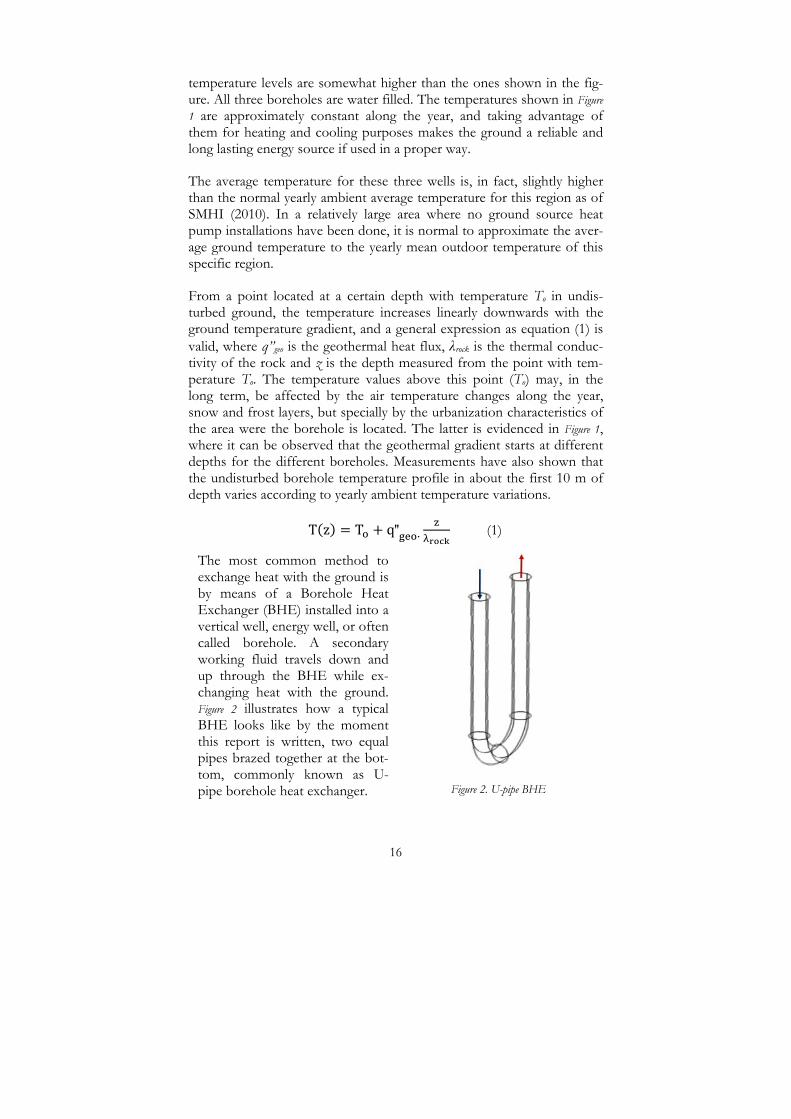
The most common method to exchange heat with the ground is by means of a Borehole Heat Exchanger (BHE) installed into a vertical well, energy well, or often called borehole. A secondary working fluid travels down and up through the BHE while ex-changing heat with the ground. Figure 2 illustrates how a typical BHE looks like by the moment this report is written, two equal pipes brazed together at the bot-tom, commonly known as U-pipe borehole heat exchanger.

Figure 2. U-pipe BHE

16

The diameter of the wells where borehole heat exchangers are normally installed is about 100 to 140 mm. The space between the BHE pipes and the borehole wall is normally filled with groundwater or other backfill material. The depth of the BHE is normally chosen depending on the demand of the application for which it is designed. The upper design limit for these systems is about 40 to 50 Watts per meter borehole, and this is set in order to guarantee the long term sustainability of the tem-perature levels the BHE. The whole depth of energy wells may, in groundwater filled boreholes, often not be utilized. Effective heat trans-fer will occur from the depth under the ground surface at which groundwater is found, determining what is called the active borehole length. Heat transfer from the rock to the secondary fluid is significantly better in this region since the thermal conductivity of water is approx-imately 20 times larger than that of air at normal borehole temperature conditions. Moreover, groundwater movement around the BHE may in-crease the convection heat transfer coefficient in the water side of the borehole. In Sweden, it is common to just leave natural groundwater around the BHE pipes. However, it is a common praxis to use other fill-ing materials in central Europe. The use of other materials instead of groundwater may improve the heat transfer and may also prevent envi-ronmental problems.

When BHE systems are used for heating purposes, the collected heat from the ground is normally delivered to the evaporator of a heat pump as the one illustrated in Figure 3, consisting of five key parts: an evapora-tor, a compressor, a condenser, an expansion valve and a refrigerant flu-id, forming a typical vapor compression cycle that upgrades and trans-ports the heat to a higher temperature level. An energy input is necessary at the compressor in order for the heat pump system to operate.

When these systems are used for heating applications, the con-nection between the borehole heat exchanger and the heat pump takes place at the evapo-rator, where the refrigerant en-ters at saturated conditions (point 1 in Figure 3) and evapo-rates as it absorbs heat from the secondary working fluid coming from the BHE loop.

Figure 3. GSHP sic sketch ba

The ratio between the heat transferred in the condenser (energy deliv-ered by the GSHP system for a certain heating application) and the ener-gy input at the compressor and circulation pumps is com-

17

18

monly known as the Coefficient of Performance (COPheating), expressed in equation (2), being asure of the overall efficiency of the system. a me

COP QE E

(2)

It can be interpreted from equation (2) that, the greater the energy input at the compressor and circulation pump, the lower the COP of the sys-tem. Striving for the reduction of these two energy inputs through un-derstanding and improving U-pipe borehole heat exchangers is the gen-eral goal of this thesis.

1 . 2 T h e r m a l P r o c e s s e s i n t h e G r o u n d

The thermal process in the rock under the ground (without groundwater movement) is governed by the three dimensional heat conduction equa-tion, as expres d w t cylind ica ordinates in equation (3). se i h r l co

(3)

If extracting heat from the ground, the temperature drop in the borehole is relatively rapid during the first hours and, in typical Swedish rocks, the steady state extraction temperature is obtained after about a couple of decades. The thermal process in the ground is mainly radial during the first years and becomes three dimensional after several years.

For steady state conditions, the Fourier’s law can be written for the heat flux q’’ between the ground and the wall of a single BHE at a cross sec-tion as in equation (4), where n represe the direction of the heat flux. nts

(4)

For a borehole of radius rbh, the thermal power per meter borehole q’ [W/m] can be written with a boundary condition of what happens just at the borehole wall (boundary between the borehole and a bit into the ground at r ≈ rbh) by multiplying equation (4) by the borehole perimeter 2πrbh, as expressed in equation (5), where ⁄ is the temperature gra-dient in the rock at the border e bo . of th rehole

/ · 2 (5)

19

When a heat extraction period in a BHE starts due to operation of a heat pump, a sudden change in the temperature levels occur in the borehole. Part of the heat that reaches the circulating fluid is heat that is stored in the different materials inside the well, e.g. pipe, groundwater/ grouting, etc. Considering these capacitive effects is important when studying the short term behaviour of these systems. However, this influence de-creases as the BHEs become more efficient since the thermal resistances in the borehole are minimized and problems depend more and more of the thermal process in the rock itself. This will be further justified and il-lustrated in this chapter when the borehole thermal resistance and the thermal response test method are introduced, given that they imply im-portant concepts that are used throughout this thesis.

For the transient response of the ground to heat pulses taking place dur-ing heat exchange periods that will perturb the ground’s temperature with certain periodicity, it can be said that the heat exchanged in the BHE is a function of time q’(t) and that this process is somehow super-posed to the natural stationary temperature distribution that previously existed in the ground. Mathematically, as expressed in Claesson et al (1985), the different heat transfer forms with origin in equation (3), are mainly linear partial differential equations for which solution of two or more temperature change processes can be superposed.

In a borehole heat exchanger submitted to a constant heat extraction rate q where Tf(t) is the mean fluid temperature along the depth as a function of time and Trock(0) the rock temperature at an initial time t=0, it is gener-ally possible to write the temperature difference between the fluid and the ground as expressed in equation (6), where Rb is the thermal resis-tance between a mean fluid heat extraction point and the borehole wall (the original form of the equation (6) will be discussed later in this report as the thermal response test method is introduced in section 1.5). The definition of the borehole thermal resistance Rb is according to Hellström (1991).

0 · · (6)

The function f(t) stands for the time dependent thermal resistance of the ground and can be ex as in e a ion (7). pressed qu t

ln 4αt

rbh2 γ (7)

As interpreted from equation (6) and (7), the temperature of the fluid and also in the surroundings of a BHE suffers dynamic changes as it is used. In addition, heat exchange periods can change with time q=q(t). The temperature in the ground can be written as a function of the radial

20

distance from the BHE and of time, and its analytical solution is applica-ble just outside the borehole and for a time greater than 5R2/α. The temperature as a function of position and time may be represented as the superposition of the different heat steps. The power for a heat step pulse can be superposed to other heat exchange periods and the total course of events around the borehole can be analyzed as a sum of many different step pulses as the ones illustrated in expression (8).

q t0 t t

q t tq t t

(8)

As expressed in equation (5), the thermal conductivity along the bore-hole is of great significance for the heat transfer and for the necessary temperature changes in the ground. It decides the heat exchange capabil-ity between the borehole and the surrounding ground. This is true for a steady and for transient thermal process. However, in the transient case, the problem is more complex since time and the thermal diffusivity must instead be considered. Also, the performance of a single BHE can be af-fected by neighbor wells.

This thesis only considers single borehole heat exchangers submitted to relatively short term heat exchange processes varying from usual heat ex-traction periods during heat pump operation to slightly longer thermal response tests. The consideration of long term effects of adjacent wells is outside the scope of this project and is thus neglected, i.e. the analyses in this thesis are done as for BHEs located in infinite rock environment.

1 . 3 S e c o n d a r y w o r k i n g f l u i d f l o w The circulating fluid in BHEs normally varies from water to an anti-freeze aqueous solution of ethanol or glycol to a certain percent, depend-ing on the rock temperature conditions at a specific location and fluid design temperatures expected for the operation of the system. In Swe-den, for example, it is common to use 30% volume concentration of ethanol, reducing the freezing point of the fluid to -15 °C and decreasing the risk of freezing problems in the cold side of the heat pump. Reduc-ing the freezing point of the fluid is the immediate consequence of using these aqueous solutions, but not the only one. The thermophysical prop-erties such as the density, specific heat, viscosity, Prandtl number, etc, al-so change as the antifreeze additive is added, meaning that the choice of fluid may have a significant influence on the system hydrodynamic and thermal performance. A significant contribution that includes the ther-mophysical properties of many other working fluids used in BHE appli-cations are known from Melinder (2007). What follows below is the hy-

21

drodynamic and thermal considerations that have been used in this thesis for the analysis of secondary fluid flows in borehole heat exchangers.

1 . 3 . 1 H y d r o d y n a m i c c o n s i d e r a t i o n s When dealing with heat transfer problems in internal fully developed flow, it is of great importance to have knowledge about whether the flow is laminar or turbulent. The velocity profile inside the tube would be pa-rabolic for a laminar flow while rather flat for the turbulent case. The limit when either of these flows occurs is identified by determining the Reynolds number (Re), normally calculated according to equation (9). For fully developed flow, the Reynolds number for which turbulence starts is 2300, although much higher numbers (Re>10000) are necessary to achieve completely turbulent conditions Incropera (2007).

The convection in the secondary fluid side during laminar flow may give rise to higher thermal resistances between the secondary fluid and the BHE pipes than in turbulent flow. Therefore, it is usually desired to keep the flow within the turbulent region (there are also certain BHEs that are designed to operate at laminar flows). However, the pumping power re-quired to induce turbulence must be regulated so that the best heat trans-fer conditions are achieved in the borehole at the lowest energy cost, i.e. using as small amount of energy as possible to pump the flow. The pumping power is proportional to the pressure drop and to the volume-tric flow rate in the BHE channels, as expressed in equation (10). The pressure drop (∆P) in the pipes occurs mainly due to friction and it is greater at higher velocities. It can be estimated for a fully developed flow w u n (11). ith eq atio

· (9) ∆ · (10) ∆ · · (11)

The estimation of the friction factor f depends on whether the flow is laminar or turbulent. This is solved by using equation (12) for laminar flows and the correlation suggested by Gnielinski (1976) for turbulent flow, e in equation (13). xpressed

(12)

(for Re≤2300)

. · . (13)

(for Re≥ 2300)

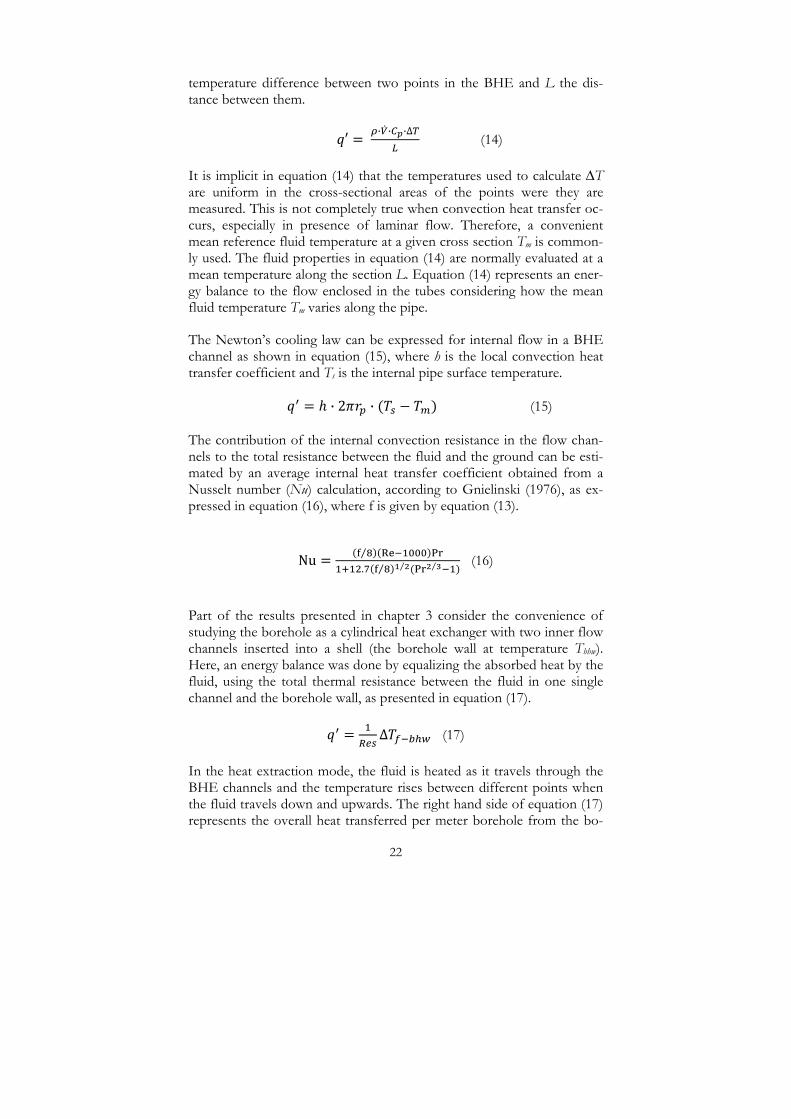
1 . 3 . 2 T h e r m a l c o n s i d e r a t i o n s The rate at which thermal energy is advected with the fluid as it moves along the pipe can be expressed as in equation (14), where ∆T is the

22

temperature difference between two points in the BHE and L the dis-tance between them.

· · ·∆ (14)

It is implicit in equation (14) that the temperatures used to calculate ∆T are uniform in the cross-sectional areas of the points were they are measured. This is not completely true when convection heat transfer oc-curs, especially in presence of laminar flow. Therefore, a convenient mean reference fluid temperature at a given cross section Tm is common-ly used. The fluid properties in equation (14) are normally evaluated at a mean temperature along the section L. Equation (14) represents an ener-gy balance to the flow enclosed in the tubes considering how the mean fluid temperature Tm varies along the pipe.

The Newton’s cooling law can be expressed for internal flow in a BHE channel as shown in equation (15), where h is the local convection heat transfer coefficien a ipe surface temperature. t nd Ts is the internal p

· 2 · (15)

The contribution of the internal convection resistance in the flow chan-nels to the total resistance between the fluid and the ground can be esti-mated by an average internal heat transfer coefficient obtained from a Nusselt number (Nu) calculation, according to Gnielinski (1976), as ex-pressed in equation (16), where f is given by equation (13).

Nu ⁄ R P. ⁄ ⁄ P ⁄ (16)

Part of the results presented in chapter 3 consider the convenience of studying the borehole as a cylindrical heat exchanger with two inner flow channels inserted into a shell (the borehole wall at temperature Tbhw). Here, an energy balance was done by equalizing the absorbed heat by the fluid, using the total thermal resistance between the fluid in one single channel and the borehol l, as sented in equation (17). e wal pre

∆ (17)

In the heat extraction mode, the fluid is heated as it travels through the BHE channels and the temperature rises between different points when the fluid travels down and upwards. The right hand side of equation (17) represents the overall heat transferred per meter borehole from the bo-

23

rehole wall to the secondary fluid, ∆ is given by the logarithmic mean temperature difference expressed in equation (18), and Res is a thermal resistance with unit [K m/W].

∆ (18)

Tin and Tout are the in and outlet temperatures in the heat exchanger sec-tion that is being analyzed. The left hand side of equation (17) represents the heat absorbed per meter by the fluid between these temperature measurement points, as given in equation (14). This heat varies in accor-dance with the flow conditions inside the collector pipes.

1 . 4 T h e r m a l R e s i s t a n c e s i n B H E s A total fluid to ground resistance (RT) consisting of the contribution of the rock thermal resistance Rrock and the borehole resistance can be de-fined between a point with mean fluid temperature and at point a undis-turbed ground condition a equation (19). s, s expressed in

RT R R (19)

As it was mentioned above, in short term transient processes, the per-formance of borehole heat exchangers with relatively low thermal resis-tance between the fluid and the borehole wall depend mostly on the time dependent thermal resistance in the rock. The time dependent thermal resistance relates the temperature evolution to steps in heat exchange rates. This is shown in section 1.5 (thermal response test) where a tem-perature increase in time during constant heat injection allows using the undisturbed ground temperature as a reference for a calculation of the temperature change due to borehole (related to Rb) and the rock thermal conductivity λrock (related with Rrock).

Nevertheless, for steady state conditions, Rrock can be calculated as for a radial system (a rock cylinder) where the inner circle is represented by the borehole wall and the outer circle is a border with undisturbed ground temperature conditions. The resistance of the rock is, in this case, a func-tion of the thermal conductivity, and the inner and outer radius of the formed ring, as follows in equation (20); rrock and rbh are the radius at the undisturbed ground co dition a rehole radius, respectively. n nd the bo

R

(20)

Since a single borehole heat exchanger is the combination of three gen-eral parts: the filling material, the BHE pipes, and the circulating fluid, Rb

is a combination of the thermal resistances associated with them, as sim-plified and illustrated in Figure 4.

Figure 4. Illustration of thermal resistance components in a BHE

Figure 4 indicates that heat is transferred through three thermal resistances between the borehole wall and the secondary fluid, each representing a temperature change. It is therefore clear that the heat transfer between the fluid and the surrounding ground depends on the thermal properties and the geometrical arrangement of the BHE pipes, the convective heat transfer on the circulating secondary fluid sides, and on the thermal properties of the filling material. The basic expressions for each of these thermal resistances in steady state conditions can be written as follows: The fluid to pipe resistance according to equation (21). Notice that this equation ima ely related with equations (15) and (16). is int t

(21) R (22)

For a single BHE pipe, normally smooth tubes made of polyethylene, the pipe thickness and the thermal conductivity (about 0.4 W/m K) deter-mines the contribution of the pipes to the borehole thermal resistance. It can be calculated as for a radial ring between the inner and outer pipe borders, as shown in equation (22). The contribution of the pipe thick-ness to the total borehole thermal resistance is reduced with increasing amount of flow channels. Figure 5 illustrates how the thermal resistance of one pipe varies with the material thermal conductivity for a typical U-pipe BHE tube thickness of 2.4 mm. The dashed line illustrates the value of most of the pipes used nowadays.

0

0,05

0,1

0,15

0,2

0,25

0 1 2 3 4

R pipe

 [Km/W

]

Thermal conductivity of the pipe [W/mK]

Figure 5. Pipe thermal resistance as a function of its thermal conductivity

It can be observed in Figure 5 that the pipe thermal resistance can be al-most eliminated with relatively low thermal conductivity material of

24

25

about 2 to 4 W/m K. Depending on the type of borehole heat exchang-er, however, it may be of interest to have a higher thermal resistance in one of the BHE shanks to reduce thermal shunt effects.

A contact thermal resistance between the borehole heat exchanger pipes and the borehole filling material, or between the filling material and the borehole wall, may also exist and thus influence the total thermal resis-tance in BHEs. This can be calculated using equation (23), being re the radius of the surface at which the contact resistance exist and δgap the width of the possible gap; λgap is the thermal conductivity of the material filling the gap.

R ln (23)

Regarding the resistance of the filling material itself, it is normally diffi-cult to estimate with good accuracy, especially in groundwater filled bo-reholes due to influence of natural convection between the BHE shanks and the borehole wall. In Sweden, mainly characterized by the presence of crystalline rock, it is common to use groundwater filled boreholes. This is, in fact, the case for almost all the installations done so far. In central Europe, on the other hand, it is normally compulsory to use backfilling materials, mainly due to water protection reasons. However, the latest standard from the Swedish Geological Survey SGU (2007) in-troduces the possibilities for eventual backfilling need. As it will be dem-onstrated in section 3.1, the thermal resistance in the filling material also depends significantly on the relative position of the BHE shanks to each other and to the borehole wall. Moreover, it is worth mentioning here that, according to Gustafsson (2006) and Gustafsson et al. (2010), the heat transfer in the groundwater side has been found to be about three times better in temperature induced natural groundwater movement as compared to stagnant water at temperature levels between 10-35˚C. This has been confirmed with numerical models and laboratory results.

As mentioned earlier, the combination of all variables in a borehole heat exchanger (including the contact resistances between the different mate-rials at the interfaces) has been simplified and defined as borehole ther-mal resistance Rb by Hellström (1991). This variable is the result of divid-ing the temperature difference (the driving force for the heat to flow) by the heat transfer rate q’ [W/m], as expressed in equation (24). Rb is a thermal resistance per unit length borehole with units [Km/W].

(24)

26

For this definition of Rb, it is assumed that the fluid temperatures of the downward and upward flow in the BHE are the same and equal to the average of these two (Tf). An undesirable phenomenon in BHEs is the thermal shunt effect between the two shanks, i.e. when heat is trans-ferred from the upcoming to the down coming pipe. Since this is a factor that compromises the heat transfer in the axial with the radial direction, this may cause temperature drop in the circulating fluid and decrease the system efficiency. Measurements that are under analysis confirm that the thermal shunt in U-pipe BHEs increases with decreasing flow rate. The thermal resistance between the down and upwards pipes must therefore be as high as possible, while the thermal resistance between either pipe and the borehole wall must be as low as possible.

A possible interpretation of equation (24) is that, for a given heat extrac-tion rate and borehole wall temperature, the BHE with the lowest Rb will deliver the highest temperature to the heat pump. Therefore, it is desira-ble to have low Rb in order to have as low temperature difference as possible between the fluid and the ground. The temperature levels in the BHE subject to a certain heat extraction or injection rate will also de-pend on the transient response of the surrounding ground (Rrock).

The borehole wall and the rock temperatures in the vicinity of the bore-hole may not vary in a symmetrical way on a 2D plane across the well, meaning that Tbhw is generally unknown. The use of equation (24) de-mands knowledge about this as well as about the local q’. Here, however, the expression is defined in order to illustrate what Rb represents. It will be shown in the next section (1.5) that it is possible to determine Rb by exchanging heat with the ground for a relatively larger time so that steady heat flux conditions are achieved. Moreover, theoretical calculations of this thermal resistance only considering steady state conduction heat transfer in chapter (3) and (4), show that it is possible to omit the prob-lem of the unsymmetrical borehole wall temperature by choosing a proper boundary with undisturbed ground conditions far enough from the borehole.

1 . 5 T h e r m a l R e s p o n s e T e s t As borehole heat exchangers constantly exchange heat with the ground, the thermal conductivity of the surrounding rock is of significant impor-tance. This property can be determined through laboratory and/or field measurements (in situ), but when the design of the BHE system is to be based on the thermal conductivity of a certain location, in situ measure-ments are a better approximation. This is due to factors that may alter the heat transfer conditions such as presence of rock fissures around the borehole, groundwater convection, borehole deviation, varying thermal

conductivity along the borehole length, among others, which make the in situ measurement would be more representative for the specific location.

An in situ method for measuring the thermal conductivity of the rock, known today as Thermal Response Test (TRT), consists of circulating a fluid through a BHE while simultaneously applying a constant heat pow-er. The first borehole thermal response tester arrangement was built to-gether with two students from The Royal Institute of Technology (KTH), Sweden, and consisted of an apparatus that delivered 2.7 kW constant cooling power to the secondary fluid in a BHE while logging the fluid temperature and the power. Figure 6 is a picture of the test rig.

Figure 6. The first Thermal Response Tester. Mogensen (1983)

The theory behind the analysis of a TRT had existed for many years. However, the work by Mogensen (1983) showed that even the borehole thermal resistance could be simultaneously determined from this analysis when carrying a TRT, rising the relevance of the results to a higher ex-tent (this is, in fact, what makes thermal response test one of the key tools for evaluating the performance of single borehole heat exchangers in this thesis). Later, at the end of the nineties, the thermal response test was further studied by Gehlin and others, e.g. Gehlin (2002).

The TRT method is widely used today, most popularly with heat injec-tion to the borehole. The supplied heat, the fluid flow, and the borehole incoming and outgoing temperatures are measured and registered. What happens during such a test is illustrated in the temperature vs. time chart shown in Figure 7. The red and the blue symbols shown on the simple TRT apparatus sketch (in the lower corner to the right) illustrate the lo-cation of the inlet and outlet temperature measurement points, respec-tively. Likewise, these two points are represented with arrows of the same color in the borehole picture shown to the left of the figure. Both temperatures are the same during the first hours of the test, where the fluid is circulated without any heat injection (this pre-circulation period is normally used to estimate the undisturbed average temperature in the

27

ground). This is followed by a temperature increase indicating that the heat injection period has started, and the difference between the bore-hole inlet and outlet temperatures is evident during the rest of the test.

Figure 7. Illustration of a heat injection thermal response test

Furthermore, the mean fluid temperature Tf is plotted in Figure 7; this has been done on purpose in order to illustrate the variable that is evaluated during most standard thermal response test analysis, known as the line source method, mathematically expressed in equation (25). This is, in fact, the original expression on which equation (6) and (7) are based. The line source model, presented by Ingersoll et al. (1948), evaluates the tem-perature response after time t of a step change in supplied heat power q. The temperature response of many such steps at different times may be superposed. The vertical yellow line along the borehole axis to the left in Figure 7 is shown in order to exemplify the source line from which heat is injected into the ground. Other mathematical models such as the cylind-er source model can also be used for the analysis of TRTs.

· · ∞

√ (25)

The duration of TRTs should be relatively long in order to achieve the appropriate conditions that allow evaluating the BHE performance in a correct way. Testing BHEs during short term heat pump cycles and rapid temperature changes is difficult due to the fact that capacitive properties may influence the results.

Thermal Response Tests allow, in this thesis, the determination of the rock thermal conductivity (λrock) and borehole thermal resistance (Rb), car-ried out by calculating the temperature difference between the fluid and the undisturbed ground as a function of time using equation (25). The

28

squared error between calculated and measured values is minimized by adjusting λrock and Rb. The integral (the exponential integral) in equation (25) is evaluated by a series expansion. Rb is an extra term added to the equation in order to account for the temperature difference between the working fluid and the borehole wall, as suggested by Mogensen (1983).

A pioneering work by Fuijii et al. (2006) using temperature mea-surements along a borehole depth allowed determining the variations in thermal conductivity of the ground along the depth. However, the evaluation of Rb was not poss-ible since the measurement points were located on the external wall of the BHE pipe, i.e. the mea-surements did not relate to the flu-id temperature Tf. Determining the borehole resistance along the bo-rehole depth is possible in this thesis thanks to Distributed tem-perature measurements inside the BHE pipes during a TRT, as illu-strated in Figure 8, a BHE with sev-eral fluid temperature measure-ment points along the depth.

Figure 8. TRT equipment connected to a borehole for DTRT

A conventional TRT (without distributed temperature measurements in the BHE) is a useful method that allows sizing of BHE installations. However, it presents merely an average thermal conductivity of the sur-rounding ground and an average borehole thermal resistance. The TRT is enhanced in this thesis by carrying out a Distributed Thermal Re-sponse Test (DTRT), i.e. measuring secondary fluid temperatures at dif-ferent depths with fiber optic cables while running a TRT. Section (1.7) explains how Distributed Temperature Sensing (DTS) technology works and chapter 2 and 4 present how the technology has been used for the analysis of DTRTs.

1 . 6 B o r e h o l e H e a t E x c h a n g e r s -s t a t e o f t h e a r t

As mentioned in section 1.1, due to relatively low costs and easiness to install, U-pipe BHEs consisting of two equal cylindrical pipes connected together at the borehole bottom have dominated in the GSHP market.

29

30

However, there are many other borehole heat exchangers types that have been tested or, at least, discussed.

Borehole heat exchanger classification is traditionally done according to the cross sectional geometry and to how the secondary fluid circulates along the flow channels, generally categorized into two types: the U-pipe (already introduced and illustrated in Figure 2), that includes different addi-tions such as double or triple configuration or spacers for separating the BHE shanks; and the Coaxial design. The latter normally consists of a central shank connected in series at the borehole bottom with one or several parallel external flow channels. The central pipe may or may not be insulated in order to avoid thermal contact with the external tubes.

U-pipe BHEs are characterized by having a poor thermal performance (high borehole thermal resistance Rb), meaning that the temperature dif-ferences between the heat carrier fluid and the surrounding bedrock are relatively large. This is mainly due to the low thermal conductivity of the pipes, thermal shunt flow between channels, and undesirable channel placement inside the borehole relative to the borehole wall. Moreover, the relatively low thermal conductivity of borehole filling materials may play an important role.

Coaxial BHE designs may offer a unique advantage if they are properly designed due to the fact that their external channel(s) are geometrically closer to the borehole wall. However, as for the U-pipe design, one of the major challenges is to avoid the thermal contact between up- and down-going channels.

This thesis presents experiences with both types of borehole heat ex-changers and what follows below is a description of the most relevant earlier research work that has been done in the Borehole heat exchanger field.

1 . 6 . 1 U - p i p e B H E s More efficient methods for exchanging heat with the ground through better BHE designs, including better ways of using the U-pipe, have been a popular thought for many years. Theoretical and experimental studies have been done.

From the theoretical point of view, a pioneering work was carried out by Claesson et al. (1987), where the heat flows between the pipes and the outer rock were computed around each of the U-pipe shanks and the outer borehole circle. The paper by Claesson et al. (1988) shows calculated borehole thermal resistances for laminar and turbulent flow in three different U-pipe configurations, even surrounded by frozen water

31

as filling material. It was clear that laminar flow in the pipes is to be avoided as it rises the value of Rb. The calculations for the unfrozen cases were done only considering conduction heat transfer, i.e. natural convection outside the U-pipe was neglected. Similar calculations to the ones done by Claesson et al. (1988) are done in this thesis applied to 13 mm and 38 mm spacers (distance between pipes) that have been provided by one of the project sponsors.

The doctoral thesis by Hellström (1991) presented several analytical equ-ations that describe the thermal processes occurring in the borehole. This work was, in fact, where the variable Rb for the borehole thermal resistance was defined. Analytical solutions of the fluid temperature pro-files and borehole thermal resistance for different BHE configurations were also considered by Zeng et al. (2003) and a recent FEM analysis presented by Esen et al. (2009) shows the two-dimensional temperature distribution at three depths of U-pipe BHEs, indicating that thermal shunt flow takes place between channels and that it becomes larger with deeper boreholes. Furthermore, Hellström (1998) presented the Rb for a single U-pipe for different borehole filling materials with three different pipe positions in the borehole.

From the experimental point of view, although Mogensen (1983) sug-gested the thermal response test method to measure the borehole ther-mal resistance in borehole heat exchangers, nothing seemed to have happened - besides the work by Eskilson et al. (1987) - regarding ex-perimental determination of Rb until Eklöf and Gehlin (1996) presented their work as a mobile equipment for carrying out such tests. The con-tinuation of the latter work resulted in the doctoral thesis by Gehlin (2002), presenting test results for U-pipe and double U-pipe BHEs and significantly contribution to the understanding of the TRT method. Also, Hellström (2000) compared Rb at different temperature levels and heat rates for groundwater filled U-pipe BHEs, among others. The results show values between 0.053 and 0.08 K m/W, indicating the influence of free convection heat transfer outside the U-pipe shanks. This range for Rb is in good accordance with the tests carried out by Gehlin (2002).

In addition, the work by Bose (2002) showed the results from five ther-mal response tests in U-pipe BHEs, where bentonite and a thermally en-hanced grout were used as backfill materials. This work included the use of a spacer, geo-clips, for separating the pipes from each other (i.e. avoid thermal shunt flow) and place them as close as possible to the borehole wall. Using clips together with thermally enhanced grout resulted in sig-nificant improvement possibilities, i.e. the clips guaranteed good separa-tion between the pipes and therefore their proximity to the borehole wall.

32

The decreasing effect of the borehole thermal resistance Rb due to free convection in groundwater filled BHEs has been shown to increase with increasing groundwater temperatures. Significant contributions to the clarification of this phenomenon have been presented by Gustafsson (2006) and Gustafsson et al. (2010). Future study of U-pipe BHEs may be focused on natural convection on the groundwater side, freezing of groundwater in BHEs, better grouting materials, and flow optimization for different borehole depths.

1 . 6 . 2 C o a x i a l B H E s Development of coaxial BHE ideas has been discussed by Platell (2006), who presented an interesting thought consisting of one central insulated pipe and several outer pipes. This design has been called TIL, after the initials of Thermal Insulated Leg. Platell (2006) shows a list of different models illustrating its thermal advantages and not least their good hy-draulic characteristic, i.e. lower pressure drop thanks to the use of lami-nar flow. A first prototype was tested and presented by Hellström et al. (2000), resulting in thermal resistances between 0.009 - 0.028 K m/W. The prototype consisted of 62 thin pipes (diameter of 3.8 mm and thick-ness of 0.65 mm) arranged close to the borehole wall in a special labora-tory installation. The diameter of the laboratory borehole was 104 mm. Preliminary recent results show thermal resistances of about 0.02 – 0.03 K m/W. Further study of this design is ongoing at the moment at KTH using Distributed temperature measurements.

Other prototypes have been suggested in Finland, consisting of one cen-tral channel and five outer channels with trapezoidal cross section. De-tails as well as simulation results from this BHE are found in the work by Andersson (2008). The first prototype of this design is tested as part of this study and it is presented in section 4.2. Further development is still ongoing.

Furthermore, a coaxial annular borehole heat exchanger was demon-strated during the EU project GROUNDHIT by Sanner et al. (2007), where even former work regarding initial ideas about coaxial borehole heat exchangers from the early 1980s is presented. Also, EWS (2006) de-scribes the GROUNDHIT design. This BHE consisted of one PE63x5.3 mm outer pipe with an inner channel with dimensions PE40x3.7mm. In-stallation and assembling methods were as well tested and presented.

Hellström (2002) described experiments with an open annular coaxial BHE where the secondary fluid travels in absolutely direct contact with the rock in the annular channel, i.e. an open groundwater system. Some operating conditions resulted in Rb values of circa 0.01 K m/W, drasti-cally lower than the one corresponding to U-pipes.

33

1 . 7 D i s t r i b u t e d T e m p e r a t u r e M e a s u r e m e n t s

Different measurement techniques and equipment have been used in the experiments presented in this thesis, e.g. distributed temperature sensing with optical fiber cables, thermocouples, resistance thermometers, pres-sure meters, loggers, groundwater level meter, and even a submersible video camera. Most of them are widely known and have been previously used in borehole heat exchanger research. However, the advantages of Distributed Temperature Sensing (DTS) have never been taken up to the extent that is used in the experiments presented in this thesis. Therefore, this sub-chapter is dedicated to giving a brief background of how this technique works. Practical details about how the measurement cables were deployed can be found in Acuña (2008).

DTS allows having a clear picture of the temperature profiles along the borehole depth by deployment of one single optic fiber cable in the well, instead of many local sensors. This cable can be used to measure the un-disturbed ground profile and the fluid temperatures while exchanging heat with the ground at almost any moment and at any local point.

The working principle of DTS technology is based on Raman optical time domain reflectometry. It consists of the injection of laser light pulses through a length of optical fiber and the subsequent detection of a non-linear part of the reflected light that is re-emitted with a different frequency than the input signal and travels back through the fiber from the observed point. This frequency shifted light scattering is called raman scattering, and the temperature is determined by analyzing it over a pe-riod of time (integratio e). n tim

·∆ (26)

The re-emitted raman scattered light has one part at lower wavelengths (stokes Is) and another at higher wavelengths (anti-stokes IA) than the original injected light. The low and high frequencies are related to the energy gap between them. The ratio between them only depends on temperature, meaning that the temperature can be determined at a cer-tain section as a function of the ratio between stokes and anti-stokes (IA/Is) backscattered light. This ratio allows compensating for the losses in the IA and Is signals.

As to Farhadiroushan (2009), the temperature at this specific section is evaluated with an expression as shown in equation (26) where Gamma (γf) is written with a sub-index in order to differentiate it from the one

the Euler’s constant in the line source model, and it is obtained accord-ing to γf = h*υ/k; h is the plank constant, υ the phonon energy band, and k the Boltzmann constant. Gamma is evaluated during the manufactur-ing calibration setup under insignificant effects of the differential loss. This is done by keeping two sections of the fiber close to the instrument at two different constant temperatures. After this, γf should not consi-derably change and is, in most cases, constant.

The ratio CA/Cs is called Ratio of intensity coefficients for anti-stokes and stokes detection and is also calibrated with reference with a section of fiber kept at a known reference temperature where the effects of losses are negligible. Later, after the system has been calibrated, this ratio can be dynamically adjusted with a known temperature reference.

The variable z is the distance along the fiber from the instrument, ∆α the differential loss between anti-stokes (αA) and stokes (αs) loss. With known travel time and velocity, it is possible to identify the position of where a signal comes from. It can be observed that the differential loss (∆α) affects the temperature reading in proportion to the distance (z) from the measurement instrument. ∆α is adjusted so that the same tem-perature is read at the beginning and at the end of the optical fiber. This loss is normally within the order of 0.3 decibels per kilometer with lasers operating at around 1064 nm.

Figure 9. The data logging equipment

Figure 10. Thermocouple con-nection sketch

The description of the test installations in the following chapters include pictures of the borehole heat exchangers where the fiber optic cables can be observed after complete installation (see Figure 14, Figure 40, Figure 65, Figure 66). The laser generation and data acquisition system in all cases looks approximately like a normal computer, as shown in Figure 9. A tempera-ture box and a data logger is also part of the measurement instrumenta-tion. These are used in order to read local temperature at certain points

34

35

of interest by using thermocouples, the working principle of which is briefly illustrated by the sketch in Figure 10. Through the temperature box, each of the thermocouples is connected to a logger by a circuit with an internal reference temperature (J2). The measurement points in the BHE are represented by the junction J1. The temperature is a function of the voltage difference, which is read and interpreted by a logger.

The precision of a DTS measurement increases with the amount of in-formation read by the data acquisition instrument per unit time and with the size (length and diameter) of the observed section along the fiber, i.e. better accuracy is obtained when more photons are observed per unit time. However, the photon density decreases with increasing length of the measurement section, meaning that the amount of information read by the instrument in a certain period of time may also be smaller if the length of the observed section is large.

In this thesis, two different DTS instruments have been used: Sentinel and Halon, both from Sensornet and with spatial resolution of one and two meters, respectively. The spatial resolution is the maximum width of a step temperature change that the instrument can detect, and it is de-fined as the distance between 10% and 90% limits of a detectable tem-perature step. The instrument integrates (sums up) the signals from this section and determines an average temperature for this length. In case there is step temperature change, e.g. a hot or cold spot in the fiber ca-ble, the width of which is lower than the instruments spatial resolution, the measured temperature is affected by a factor approximately propor-tional to the ratio between the spot width and the spatial resolution.

Moreover, the light signal becomes exponentially weaker as it travels through the fiber, meaning that the amount of information coming back to the DTS instrument decreases with the distance at which a measure-ment is to be taken, i.e. a section of the fiber located far away from the instrument needs a longer integration time. As a conclusion, for a given fiber optic cable, the expected precisions for temperature, time, and space, must be compromised in order to achieve the desired measure-ment quality.

The intensity of the laser is diverse for different DTS instruments and the fiber characteristics change manufacturer to manufacturer. In order to guarantee quality on distributed temperature measurements, a careful calibration process must be carried out. This normally requires the ad-justment of an offset and a slope correction during the calibration process in order to compensate for the losses along the cable length. Since the Borehole Heat Exchanger research installations in this thesis demanded special installation procedures and subsequent fiber and con-

nector splicing, the calibration process has been carried out after the bo-rehole heat exchanger installation and instrumentation was done, nor-mally under undisturbed ground temperatures conditions. This post-installation calibration process have consisted of placing two relatively long cable sections (separated from each other as much as possible) into one or even two environments with a known temperature such as an ice bath, by rolling together several meters of cable normally located before and after the borehole loop, as illustrated in Figure 11. The ice-bath ar-rangement was also insulated on the top.

Figure 11. Ice bath for fiber optic calibration

Figure 12 illustrates, as an example, the fiber cable loop from one of the re-search installations studied in this thesis. In this case, two BHEs are in-strumented with this technology and a common box is used to weld the different loops so that simultaneous measurements in both boreholes is possible.

36

Figure 12. Sketch of the fiber optic loop in two BHEs

The box where the loops are welded together in Figure 12 is, in this case, the link between the whole cable measurement length and the integration instrument (DTS shown in Figure 9). The numbers denoted with the tag LM:X are marks that delimit the beginning, bottom, and end of a certain

borehole loop. The cable length between these marks and the welding box (or the instrument) is the one inserted into the ice bath for calibra-tion purposes.

0

1

2

3

4

5

6

7

8

9

10

0 50 100 150 200 250 300 350 400 450 500

Tempe

rature [˚C]

Cable length [m]

Figure 13. Example of DTS measurement during calibration

Figure 13 shows a measurement carried out in a borehole heat exchanger during undisturbed ground temperature conditions using a calibration with the ice-bath. In this case, the BHE is 190 m deep and its undis-turbed temperature levels are observed between 50 and about 240 meters with an average of about 8.5˚C. The symmetry of the measurement (with symmetry line at about 240 m) is due to the fact that the cable goes down and up through the down and upwards channels of the BHE. The temperature levels were calibrated with an offset by considering the tem-peratures of two 40 meter long cable sections inserted into ice-baths as the ones illustrated in Figure 11, located in the interval 10-50 m and about 420-460 m. These two sections show a temperature of almost 0˚C.

Last but not least, besides the considerations mentioned above regarding the instrument and calibration, another factor that may be of relevance when measuring with DTS in borehole heat exchangers is the cable loca-tion inside the pipe.

As it was presented in section 1.3, the flow pattern in BHE pipes may be laminar or turbulent. This depends mainly on the fluid itself and its properties at a given temperature level, as well as on the volumetric flow rate. The fluid temperature distribution in a cross section of any BHE pipe changes depending on the flow regime. After a BHE has been in-strumented with fiber optic cables and/or thermocouples for measure-

37

38

ments of the secondary fluid temperature, the lateral position of the fiber optic cable and the location of the thermocouple junction inside the BHE pipes is normally unknown, raising the question about how the temperature readings may be affected by the position of the cable.

Given that there is a laminar sub-layer at the pipe wall, its thickness (δ) can be estimated and, since heat is only transferred by thermal conduc-tion within this sub-layer, δ can be used to calculate the temperature dif-ference between the pipe wall and the inner border of the boundary layer (ΔTconduction) with equation (4) using the boundary layer thickness instead of an arbitrary direction. Moreover, given that the pipe dimensions, the fluid thermophysical properties, the fluid velocity, and the heat flux from/to the ground are known, it is also possible to estimate the convec-tion heat transfer coefficient and thereby, with equation (15), the tem-perature difference between the pipe wall and the bulk fluid temperature (ΔTconvection). The comparison of ΔTconduction and ΔTconvection gives an indication of where across the pipe the temperature change take place during lami-nar or turbulent flow, varying depending on the flow regime. For turbu-lent flow, for instance, it is well known that the temperature profile is flat across the pipe after the thermal boundary layer. If ΔTconduction and ΔTconvection are similar, most of the temperature change occurs thus in the laminar sub-layer. If the fiber optic cable radius (the measuring fiber is located in the center) is larger than the layer thickness δ, the measured temperature would certainly correspond to the fluid bulk temperature.

Fiber optic cables may differ in diameters and the cable specifications vary from manufacturer to manufacturer. It is important to study the sui-tability of this measurement technique for every specific case so that an acceptable accuracy is reached. In case of the measurements with ther-mocouples, the measurement junction was installed striving for it to be located as close to the pipe center as possible in order to ensure that the bulk temperature is measured. Details about this measurement technique are described in detail in Acuña (2008).

39

2 Experiences with U-pipe BHEs

2 . 1 D e s c r i p t i o n o f t h e i n s t a l l a t i o n The evaluated borehole is located in the south of Stockholm, Sweden, at an installation with a total of 6 boreholes separated from each other at the surface level by at least 4 meters. The borehole diameter is 140 mm and its total length is 260 m. Its ground water level oscillates around 5.5 m, giving an active borehole length of approximately 254.5 m. A polye-thylene U-pipe BHE of the type PE 40x2.4 mm has been installed and filled with an aqueous solution of 20% ethanol volume concentration, providing a freezing point of -8°C according to Melinder (2007). The ex-act length of the U-pipe collector is 257 meters since some extra weight was added to the collector bottom during its installation.

For the temperature measurements, the borehole is instrumented on the groundwater and the secondary fluid side with optic fiber cables (50/125 - graded index - Multimode) for Distributed Temperature Sensing. Two different reading equipments have been used, Sentinel-DTS and HA-LOn, both from Sensornet. These instruments can examine the tempera-ture distribution along the entire cable length, with a spatial resolution of 1 m and 2 m, respectively.

On the secondary fluid side, T type stainless steel sheathed thermo-couples are also inserted into the pipes at 15, 55, 130, 220 m in each tube and at the collector bottom. The thermocouple cables are taken to the top of the borehole and connected, through a temperature box (which contains a circuit with an internal reference given by a Pt-100 sensor), to an Agilent data acquisition unit that reads the measurements. Figure 14 shows an overview of the borehole seen from the top where the sensor cables can be observed as well as the connection between the U-pipe with the insulated pipes through which the secondary fluid is transported towards and from the heat pump.

Figure 14. Overview of the borehole components

The deviation of the borehole with respect to the vertical direction was measured with an instrument of the type FLEXIT MultiSmart, an in-strument that orientates itself after the earth magnetic field as it is sent down into the borehole and registers the dip (the inclination between 0 and +/- 90°), and the azimuth (the direction between 0 and 360° relative to the earth magnetic north) angles. With these, the Cartesian position parameters x, y and z, are calculated at each measurement point. Mea-surements were taken every 10 meters over the whole borehole length, for a total of 26 measurement points. Figure 15 shows the results plotted for the x (northward) and y (eastward) directions, indicating that the bo-rehole is deviated 56.4 m and 30.5 m towards east and north, respective-ly, when measuring 260 meters away from the top.

Figure 16 illustrates the deviation of the borehole (denoted with the name BH4) together with other neighbor boreholes. The black lines represent the expected vertical direction down to 260 meters deep. It can be ob-served that BH4 did not reach the desired depth. Instead, the end of the borehole is 9.65 m above the expected level. The borehole deviation in-creased while drilling which might normally be the usual case. It may thus be of convenience to refer to borehole length instead of borehole depth regarding the total distance from the borehole top to the bottom.

During the deviation measurements, the temperature of the ground was also registered at the 26 points. These measurements are presented in Figure 18 together with temperature measurements with the optic fiber ca-ble.

40

Figure 15. Deviation of the borehole towards north and east direction

Figure 16. Deviation of the borehole with regard to the vertical direction

As it can be seen in Figure 16, boreholes are often not vertical and normal-ly deviate from this direction. The deviations may be due to presence of rock fissures that suddenly change the drilling orientation, as well as to the drilling methods and equipment. The deviation might cause that the BHE pipes rest on one of the borehole sides, tending to have contact with the borehole wall to a certain extent. The deviation also implies that the BHE pipes do not reach the desired depth.

Maps from the Geological Survey of Sweden SGU (2008) state that the average constant possible groundwater extraction in the region where this BHE is located is under 10 liters/minute, being an indication of what groundwater flow magnitudes could be expected. However, in or-der to be able to explaining possible deviations in temperature measure-ments that are found in this borehole (see following sections), a detailed groundwater flow test was done along the borehole depth. This mea-surement is done by pumping out water at a sufficiently low flow so that the ground water level stays constant due to its balance with the bore-hole incoming groundwater. The flow at different depths is measured with a flow logging equipment from GEOSIGMA AB, basically consist-ing of a cylindrical probe with an inbuilt propeller located in its inner part. More details about the instrument can be found in Acuña (2008). The groundwater flow measurement is carried out by decreasing the wa-ter level in the borehole so that an inward water flow is created, and then sending down the probe at a known velocity and registering the rotation rate of a propeller which might vary due to the presence of local

41

groundwater flow at certain sections of the borehole. The propeller rota-tion is registered and subsequently related to the groundwater flow con-ditions. The results are shown in Figure 17. The flow logging activity could not be carried out either when keeping the groundwater level at its origi-nal conditions nor when it was lowered to 22 m. The water level was then reduced to 35 m with respect to its original level and, at this point, although the current flow was low, a logging process was carried out. It is observed that a lower flow value was registered between 190 and 200 m. The borehole is considered to be tight and without presence of signif-icant groundwater flow, as it was about 0.4 l/min along the depth after decreasing the ground water level by 35 meters from the original level.

Figure 17. Ground water flow along the borehole length

Figure 18. Undisturbed Tem-perature profile

The minimum allowable ground water flow value for finding anomalies (fractures, fissures, cracks) for this equipment is 2 l/min. Therefore, no anomalies were localized during the test. However, the results show that there is a possible small increase in the borehole diameter at a depth be-tween 190 and 200 m since a lower flow was registered.

42

43

Regarding the undisturbed ground temperature levels in the borehole, it was measured before the BHE was put in operation, every 5 minutes during eight hours with the optic fiber cable installed between the BHE and the rock. The total measured borehole length is 247.8 meters (the fi-ber does not reach the total borehole length) and the results of the mea-surements are shown in Figure 18. It can be observed that the temperature increases approximately 2.5 degrees in the first 10 meters. The tempera-ture gradient between 10 and 110 meters is negative, i.e. the temperature decreases in the region from 10.5 to 8.7 °C. At this depth (110 m), the undisturbed ground temperature has a minimum and then, the gradient becomes positive (approximately 0.01K/m) for the remaining length.

As mentioned above, the groundwater level in this borehole is around 5.5 m under the surface. The lower temperature levels at the top of the borehole are justified by the fact that the undisturbed ground tempera-ture measurement was done during a colder season. Moreover, the un-disturbed profile measured every 10 meters during a relatively warmer season with the FLEXIT instrument (while measuring the borehole dev-iation) show, in Figure 18, the same general profile. The seasonal tempera-ture difference close to the ground surface is evident, as compared with the fiber optic measurement. The minimum temperature with this in-strument is registered at a depth between 140 and 150 m. The tempera-ture resolution of the FLEXIT instrument is 0.5 °C while for the fiber optics it is 0.02 °C, which partially explains the difference between the two measurement methods.

2 . 2 T e m p e r a t u r e s d u r i n g H e a t P u m p o p e r a t i o n

As already mentioned the borehole is instrumented on the groundwater and the secondary fluid side with optical fibers and also with T type stainless steel sheathed thermocouples located in the center of the pipes at different depths for temperature measurements.

The internal fiber optic cable measures the secondary fluid temperature along the whole collector length whilst the external cable measures the groundwater temperature until a depth of 247.8 meters. The DTS equipment is configured to measure every one meter and therefore, ap-proximately 257 measurement points are taken in each collector pipe. Since the external fiber cable is doubled, the total amount of measure-ment points in the ground water side is 496. Moreover, temperature measurements are taken with thermocouples located at 15, 55, 130, 220 meters depth, and at the collector bottom.

Figure 19 is an example of temperature measurements carried out with thermocouples at different points along this U-pipe BHE, showing that a temperature drop occurs in all the thermocouples following the flow di-rection as the heat pump starts operating. The heat pump takes heat from the borehole and the temperatures increase as the fluid travels along the BHE: the first thermocouple, at 15 m depth on the downward flow, is the earliest point to register the heat pump start up. Conversely, the last thermocouple at 15 m depth on the upward flow, notices the heat pump about 1/5 of hour after. For this case, the total temperature change is of about 3.6°C, an increase of three degrees on the way down and of one degree on the way up. The heat distribution in the borehole (equivalent to the temperature difference between measurement points) varies according to how fast the fluid is traveling. The duration of each heat pump cycle will vary according to the outdoor temperature and the building energy demand. The fluid temperature at all points in Figure 19 is higher than the ambient temperature for this measurement period, de-monstrating one of the strongest features of GSHPs, keeping stable and relatively higher source temperatures regardless of the ambient condi-tions.

-2

-1

0

1

2

3

4

5

0 1 2 3 4 5 6 7 8 9 10

Tem

pera

ture

[C

]

time [hour]Outdoor 15m down 55m down 220m downbottom 220m up 55m up 15m up

Figure 19. Fluid temperatures at different depths during heat pump operation

Moreover, Figure 20 shows typical temperatures in the borehole while ex-tracting heat from the ground, this time measured with the optic fiber cables. It can be observed that the fluid temperature constantly increases during its trajectory through the BHE. The inlet and outlet temperatures are in this operating case about 0.6°C and 4.4°C, respectively, while the corresponding value at the collector bottom is 3.4°C.

44

Figure 20. Temperature profile during heat pump operation

The fluid temperature change on the way down to the BHE bottom in Figure 20 is again significantly higher compared to the up going flow. As mentioned above, the shape of this temperature profile will look differ-ent at different volumetric flow rates. The groundwater temperature os-cillates between 4.5°C and 6°C. The latter is accredited to the fact that the exact location of the optic fiber cable in the borehole is unknown, i.e. the cable might be located close to the borehole wall at some points whilst next to the BHE wall at some others (it will be shown later in this thesis – chapter 4 - that it is possible to control the location of the exter-nal fiber optic by forcing to be in contact with the borehole wall with help of a so called energy capsule).

The difference between the readings from the thermocouples and the fi-ber optics in Figure 20 is 0.7 °C in the worst case. This could be in part at-tributed to the location of the measurement point. According to Acuña (2008), the thermocouple measurement point is located striving for it to be close to the middle of the tube. The optic fiber cable, on the other hand, can be located anywhere inside the pipe. Possibly, conduction through the thermocouple steel wire could influence the measurement.

When making continuous measurements with optic fibers, it is possible to have a detailed picture of the temperature changes at any borehole lo-cation during any specific time. Figure 21 illustrates the secondary fluid temperature change in the down going pipe during a typical operation cycle of the borehole. These measurements were taken every two mi-nutes for a period of 2 hours during the 3rd operation day of the system.

45

It can be observed that, during the period between 0 and 20 minutes, the heat pump is in operation and the fluid temperature goes from 0 to ap-proximately 4°C between the top and the bottom of the collector. This profile changes slowly between the minute 20 and 80, when the heat pump is not in operation. Then, the temperatures along the borehole start to balance themselves becoming warmer until almost the whole bo-rehole has an average temperature of about 5°C.

Figure 21. Secondary fluid temperature profile during borehole operation cycle

In Figure 21, the heat pump starts once again during the last 30 minutes and the borehole temperature changes first take place at the upper part of the BHE and propagate with time to the collector bottom. The latter is also illustrated for the same period in Figure 22, where it is observed that the secondary fluid temperature during minute zero is approximately the same as for the groundwater over the whole borehole length (about 6°C) and that the temperature difference between the borehole inlet and out-let changes as soon as the heat pump starts to extract the energy from the secondary fluid. Most of the energy (approximately 65%) is again col-lected in the down going pipe while the rest is collected when the fluid is coming back up towards the borehole top. At these working conditions, the fluid temperature increases almost always along the borehole length after the first 4 minutes of operation.

46

Figure 22. Fluid and ground water temperatures during the system start up

A first step into the analysis of such temperature profiles has been done by observing temperature measurements at different volumetric flow rates only with the thermocouples. Hence, the effect of the mass flow rate on the relative distribution of the specific heat extraction along the borehole depth can be studied in a straight forward way. Measurements have been taken at three different flow rates of approximately 0.3 l/s, 0.4 l/s, and 0.5 l/s.

In order to measure and adjust the fluid mass flow rate, the borehole loop is also instrumented with an inductive flow meter of the type Bru-nata HGS9-R6 and a STA-D regulation valve, both located in the return line. In addition, closing and/or opening neighboring boreholes and a frequency controlled circulation pump are used for flow regulation pur-poses.

The temperatures have been measured with the eight thermocouples every minute during heat pump operation. The thermocouples are this time denoted as T1 and T9 (at 15 m), T2 and T8 (at 55 m), T3 and T7 (at 130 m), T4 and T6 (220 m), as well as one at the collector bottom (T5). Unfortunately, T4 broke during the BHE installation and no readings are presented for this point. The thermocouples have been named according to the flow direction, i.e. T1 and T9 are the first and last measurement points, respectively. For practical reasons, the flow direction has been inverted when comparing with Figure 20.

47

Figure 23. Temperatures and specific heat extraction at 0.3 l/s

Figure 24. Temperatures and specific heat extraction at 0.4 l/s

Figure 25. Temperatures and specific heat extraction at 0.5 l/s

An instant for a heat pump cycle with stable temperature conditions (moments at which the temperature differences along the BHE are con-

48

49

stant in time during a heat pump cycle) at each flow has been chosen for this study. The fluid density, kinematic viscosity and heat capacity are calculated based on Melinder (2007) at the average temperature. Figure 23, Figure 24, and Figure 25 show a summary of the measured temperatures and the calculated specific heat extracted along the BHE pipes for seven sec-tions at the three flow rates. The latter has been calculated using equa-tion (14). The evolution of the temperature along the whole collector is clearly observed for each case. The temperature levels in the borehole will certainly decrease with time as the heat pump is in operation, but the relative relation among temperature levels at the same flow rate will re-main similar if no changes of the conduction/convection conditions on the groundwater side of the BHE take place.

It can be observed in Figure 23, Figure 24, and Figure 25, that the temperature levels are different for each of the three cases. This is due to the fact that the experiments were carried out during different days and with different flow regulation strategies; the temperature change between T1 and T9 (points closest to the heat pump evaporator) also varies for the three cases. The test installation has 6 boreholes and, as mentioned above, the flow was regulated through either adjusting the valve, the frequency of the circulation pump, and/or the simultaneous operation of the adjacent boreholes), meaning that the total flow (sum of flows in all boreholes) passing through the heat pump evaporator would determine the total temperature change in the borehole loop. A case with a single borehole submitted to a constant evaporator cooling capacity would not have pre-sented the same behaviour since the total temperature change would have decreased as the brine flow rate increases.

For all three cases, the temperature rise along the BHE pipes becomes weaker as the fluid travels between the borehole inlet and outlet. For the flow 0.3 l/s, for example, the fluid reaches its maximum temperature at the point T7, from which it starts cooling down, meaning that no heat extraction from the borehole takes place after this point in the up-going pipe. Thermal contact between pipes is observed and the groundwater temperature is presumably lower in this section than the one correspond-ing to the upwards flow. This may also be the case for the two higher flow rates, but the thermal shunt flow effect is evident to a lower extent. The observation and comparison of the relative temperature change be-tween T1-T5 with T5-T9 illustrates the proportion of heat absorbed by the fluid when travelling down and upwards, and the degree of symmetry between these. It is evident, in these three cases, the temperature vs. depth curve is most symmetric for the 0.5 l/s flow, i.e. the temperature profile between T5-T9 becomes more similar to T1-T5. Therefore, the thermal influence between the U-pipe BHE channels increases with de-creasing volumetric flow rate.

2 . 3 D i s t r i b u t e d T h e r m a l R e s p o n s e T e s t

This U-pipe BHE has also been studied through a thermal response test. In this case, such test has been done with the help of distributed temper-ature measurements, a Distributed Thermal Response Test (DTRT). This test lasted approximately 160 hours and it was carried out with a new simple TRT apparatus, as the one shown in Figure 8, consisting of a circulation pump of the type Magna 25-100 from Grundfos, an inductive flow and energy meter of the type HGS9-R6 from Brunata, a STAD flow regulation valve, and an electric heater with adjustable heating pow-er between 3 and 12 kW.

The flow rate was 1.87 m3/h (about 0.5 l/s), and it was held constant during the DTRT.

The borehole was divided into 12 sections of 20 meters each as shown in Figure 26, in which the thermal conductivities and bore-hole thermal resistances were de-termined. The first section starts at 10 meters depth and the last sec-tion ends at 250 m depth, meas-ured from the ground surface. The first ten meters were neglected, since there is a portion of the opt-ical fiber cable exposed to ambient air. Neglecting the last ten meters eliminates influence of hemispher-ical heat transfer around the bore-hole bottom, which would cause deviation from the line source theory explained in section 1.5.

Figure 26. Borehole Sectioning

The temperature readout equipment used in this test is of the type HA-LO-DTS. Thermocouples inserted at different depths into the BHE pipes have also been used in this study as an extra tool to confirm the fi-ber measurements. The temperature was integrated in 10 m sections along the whole collector length, i.e. there are a total of six measurement points in each section (three in each pipe). The measurements were taken with an integrating time of 5 minutes during four continuous test phases.

50

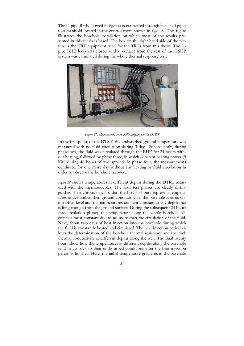
The U-pipe BHE showed in Figure 14 is connected through insulated pipes to a manifold located in the control room shown in Figure 27. This figure illustrates the borehole installation on which most of the results pre-sented in this thesis is based. The box on the right hand side of the pic-ture is the TRT equipment used for the TRTs from this thesis. The U-pipe BHE loop was closed so that contact from the rest of the GSHP system was eliminated during the whole thermal response test.

Figure 27. Measurement room while carrying out the DTRT

In the first phase of the DTRT, the undisturbed ground temperature was measured with no fluid circulation during 3 days. Subsequently, during phase two, the fluid was circulated through the BHE for 24 hours with-out heating, followed by phase three, in which constant heating power (9 kW) during 48 hours of was applied. In phase four, the measurements continued for one more day without any heating or fluid circulation in order to observe the borehole recovery.

Figure 28 shows temperatures at different depths during the DTRT meas-ured with the thermocouples. The four test phases are clearly distin-guished. In a chronological order, the first 65 hours represent tempera-tures under undisturbed ground conditions, i.e. the borehole is at its un-disturbed level and the temperatures are kept constant at any depth that is long enough from the ground surface. During the subsequent 24 hours (pre-circulation phase), the temperature along the whole borehole be-comes almost constant due to no more than the circulation of the fluid. Next, about two days of heat injection into the borehole during which the fluid is constantly heated and circulated. The heat injection period al-lows the determination of the borehole thermal resistance and the rock thermal conductivity at different depths along the well. The final twenty hours show how the temperatures at different depths along the borehole tend to go back to their undisturbed conditions after the heat injection period is finished. Here, the radial temperature gradients in the borehole

51

are very small, making it also possible to determine the ground thermal conductivity variations along the depth.

8

9

10

11

12

13

14

15

16

17

18

19

20

0 10 20 30 40 50 60 70 80 90 100 110 120 130 140 150 160

Tem

pera

ture

[°C

]

Time [h]15m down 55m down 220m down bottom220m up 130m up 55m up 15m up

Figure 28. Temperatures measured with the thermocouples during the DTRT

Equation (25) is applied to each 20 m section of the borehole, and for each section the heating power q’ is calculated with equation (14), where the fluid temperature difference ΔT is taken in each pipe at the section entrance and exit, respectively. These points also delimit consecutive sec-tions and are enumerated F1 to F26 following the flow direction, as illu-strated in Figure 26.

Figure 29 presents average temperature profiles during the first three phas-es of the DTRT. It can be observed that the undisturbed temperature profile has an average of about 9.10 °C. From the temperatures during the fluid pre-circulation phase of the test, it can be seen that the fluid adopts quite a constant temperature along the whole depth with an aver-age of 9.19 °C. Most of this temperature increase can be attributed to the circulation pump work. This constant temperature along the borehole, being an approximate mean of the undisturbed ground profile, was ex-pected to occur.

As presented in chapter 1, the undisturbed ground temperature profile may have different shapes. Sometimes, it is possible to estimate that the undisturbed average temperature is more or less equal to the one at the middle of the borehole. However, it is important to keep in mind that the undisturbed profile also depends on the urbanization characteristics

52

of the area where the well is, meaning that this may not always be the truth. The circulating secondary fluid in BHEs is exposed to the true gradient and its temperature will thus depend on this.

Figure 29. Average temperatures during the first three phases of the DTRT

Figure 29 also shows the average temperatures during the heating phase, il-lustrating that the true average temperature in the borehole is far away from the mean of in- and outlet temperature (as assumed during conven-tional TRTs). Temperature measurement in at least a few points at dif-ferent depths in the BHE would allow a better estimate of the average temperature. The latter would of course depend on which volumetric flow rate is used during the test as well as on the borehole depth.

All measurement points from each section were used for the estimation of the sectional mean fluid temperature (Tf). Regarding the undisturbed ground temperature (Trock), Gehlin et al. (2003) point out that different Trock values are obtained depending on measurement circumstances. In this case, we have used the truly undisturbed ground temperature (illu-strated in Figure 29) for each section, in order to later, during the pre-circulation period, account for the heat flow between sections and the friction heat caused by pumping the fluid. Trock is therefore not the same for all sections.

Regarding the accuracy of the measurements with the fiber optic cable during the heat injection process, the lateral position of the cable inside the U-pipe is unknown, as explained in 1.7; and the question regarding the significance of the temperature readings depending on the position of the cable must be solved. The flow pattern in the pipe is turbulent with a Reynolds number between 6500 and 8900 (fluid temperature va-

53

ries between 9 and 18°C). The laminar sub-layer at the pipe wall has, in this case, a thickness between 0.3 and 0.4 mm Schlichting (1979). In that layer heat transfer can only occur by thermal conduction. The heat trans-fer coefficient at the wall can be calculated to 1130 - 1380 W/m2 K. With a heat flux of 180 W/m2, it is found that the temperature difference between the pipe wall and the fluid (bulk temperature) is close to 0.15 K. According to Melinder (2007) the thermal conductivity of the fluid is 0.49 W/m K. Within the laminar sub-layer the temperature drop is then circa 0.14 K, thus practically the whole temperature drop occurs in this thin layer and the temperature profile in the rest of the fluid is very flat. The diameter of the fiber optic cable is 3.8 mm and thus, it measures the bulk temperature of the fluid with sufficient accuracy for our purpose.

Figure 30 presents the supplied power to the sections during the heat injec-tion phase. It is observed that power is neither the same nor constant in each borehole section during the whole DTRT. Different borehole thermal resistances between sections and differences in rock thermal conductivity will show up here. Several disturbing factors are present such as variations in the applied heating power and uncertainties in tem-perature measurements. The fluid temperature difference over a section is only about 0.15 K getting smaller for deeper sections, thus increasing sensitivity to temperature measurement deviations. A local disturbance in the common temperature measurement point at 170 m is probably the reason for the deviation in temperature observed in Figure 29 and power (between section 8 and 9) in Figure 30.

Figure 30. Power supplied in each BHE section during the heating phase

Figure 31 shows the temperature in each section during part of the heat in-jection phase (Rb is evaluated from 106 to 138 hours). The differences in temperature level between subsequent sections decreases with depth,

54

showing good accordance with Figure 29. The irregular pattern of the curves is attributed to input power variations. It is observed that the slope of the curves is fairly similar, giving an indication that the sur-rounding rock is reasonably homogeneous. Variations in Rb would move the curves either up or down, without a change of the slope, as would be the case with a change in λrock.

Figure 31. Average temperatures in each section during the heat injection phase

Figure 32 presents the average fluid temperatures in each section during the last 20 hours of the test, showing part of the borehole recovery period. Some of the section curves intersect others, while approaching the origi-nal undisturbed ground temperatures. Slight slope differences between certain sections are observed. The last 10 hours of this period (155 to 165 hours) were used for optimizing the λrock for each section.

Figure 32. Average temperatures in each section during the borehole recovery phase

55

A two step method is used for the determination of λrock and Rb; The former was evaluated during the recovery phase, neglecting the first 15 hours. This phase gives the best information about the rock thermal conductivity, since the radial temperature gradients in the borehole are low, thus virtually eliminating the uncertainty caused by the unknown positions of the BHE pipes at different depths. The results were then used as an input to calculate Rb during the heating phase, again neglect-ing the first 15 hours. Moreover, in order to account for previous heat extraction in the borehole, the undisturbed ground temperature was ad-justed by adding an experimental slope factor to the measured values.

The borehole thermal resistance and rock thermal conductivity in each borehole section are presented in Figure 33 (a) and (b), respectively.

Figure 33. (a)Thermal resistance and (b)Thermal conductivity in each section

The borehole thermal resistance varies within the range 0.054 to 0.078 Km/W, indicating changes of the pipes position in the borehole along

56

57

the borehole depth. By averaging all the Rb values we obtain a mean equal to 0.062 Km/W.

The rock thermal conductivity values range between 2.60 and 3.62 W/Km, and the result of averaging all the sections is equal to 3.10 W/Km.

Section 8 and section 9 show extreme values in opposite directions, par-tially explained once again by the deviation of the temperature measure-ment at 170 m. This may be related to the anomaly detected in the bore-hole during the differential groundwater flow measurements (Figure 17).

The average λrock and Rb obtained in the DTRT were compared with those from a conventional TRT analysis. The latter would use the fluid mean temperature at the borehole in- and outlet for the evaluation of the thermal response, as explained in section 1.5 and illustrate in Figure 7. In this case, this would correspond to the average between F1 and F26 (see Figure 26 and Figure 29). Both λrock and Rb were evaluated based on this tem-perature during the heat injection phase and omitting the first 15 hours. The result was 3.08 W/Km and 0.079 Km/W for λrock and Rb, respective-ly. Almost no deviation from the DTRT regarding λrock was found. How-ever, the Rb value corresponding to the conventional TRT test deviates from the DTRT average result by circa +28 %. The deviation is caused by the overestimation of Tf in using the mean of in- and outlet tempera-tures instead of an average over the whole borehole (Figure 29). Using this average will yield an Rb equal to 0.063 K m/W and the same value for λrock as before. This suggests that adjustments should be made to conven-tional TRT evaluations in order not to overestimate the borehole thermal resistance.

2 . 4 D i s t r i b u t e d P r e s s u r e M e a s u r e m e n t s

Earlier secondary fluid temperature measurements at different depths in a U-pipe BHE have indicated that the heat transfer in some sections is lower than expected. Some hypothesis state that this is due to the fact that flow has been laminar at Reynolds numbers where turbulent flows are expected. The measurements presented in this sub-section have as objective to measure in detail the pressure drop in U-pipe BHE pipes in order to have a clear picture of flow regime transitions, done by measur-ing pressure drop along a horizontal pipe where an aqueous solution of Propylene glycol with 32% weight concentration (-14°C freezing point) is circulated at different flows. The experimental rig consists of a PE40x2, 4 mm U-pipe. Forty pressure tabs for pressure measurements are located along the pipe with 5 meters distance between them. There

are 212 meters of pipe length between the first and last pressure tab. The loop has a 180 degree bend after pressure tap number 20, i.e. there are 20 measurement points before and 20 after the bend. Figure 34 illustrates the experimental rig, and the pressure tabs (valve) were installed as illu-strated in Figure 35. The rig also contains a Pump Magna 25-100 (Grund-fos), a Brunata HGSR9 flow meter/temperature measurement, an STAD TA regulation valve, a Filter, and a Spirovent microbubble deaerator.

Figure 34. Distributed pressure measurement experimental rig

*picture by Lukas Schlichtmann

Figure 35. Illustration and picture of the pressure tabs

Initially, the pressures were measured during no flow circulation in order to later be able account for the height difference between the measure-ment points. A height difference of about 60 cm (6 kPa) between points 1 and 40 with respect to points 20 and 21 was identified.

Subsequently, pressure measurements were carried out at seven different volumetric flows, tabulated in Table 1, where the average temperature at each of the measurement occasion is also shown together with the ther-mophysical properties used during the calculations.

Table 1. Flows and fluid properties during the tests

Flows [l/s] Working Temp [°C] Density [Kg/m3] Kin. Visc [mm2/s]

0.15 17 1027 3.51 0.2 16.8 1027 3.53 0.3 15.8 1027 3.68 0.4 17 1027 3.51 0.5 16.8 1027 3.53 0.6 16.8 1027 3.53 0.7 15.8 1027 3.68

58

The instrument used to measure the pressure is of the type TESTO 526-2. It measures pressure differ-ences within the range of 0 to 2000 hPa with an accuracy of +/- 0,05 % of the full scale value. It was connected during the meas-urements to a sealed cylindrical transparent tube through a flexible hose and from there to the pres-sure tabs, as illustrated in Figure 36.

Figure 37 and Figure 38 show the measured pressures at all flows be-fore and after accounting for the height differences between meas-urement points.

Figure 36. Connection of the pressure meter to the pipe

Figure 37. Pressure values before subtracting the height difference between points

After subtracting the height differences at each point from the measure-ments in Figure 37, it is possible to appreciate in Figure 38 the relation be-tween the line slopes before and after the bend for each of the volumet-ric flows. The tendency is the same for both sections, meaning that the flow regime behaviour tends to be the same before and after the bend.

The slightly larger pressure drop between point 20 and 21 is due to the extra loss in the U-pipe bend. It is worth to remark here the importance of following the welding standards for the bottom part BHEs. Practical experiences during this research have shown that the cross section of the pipe may be drastically reduced depending on the welding quality. The

59

total pressure drop in the loop may be affected by this. This situation changes from pipe to pipe, and from manufacturer to manufacturer.

Figure 38. Pressure values accounting for the height difference between points

Table 2 presents the experimental and theoretical pressure drop between pressure tab number 1 and number 40, i.e. between the first and last measurement points. The theoretical pressure drop was calculated with the equation (11), where the friction factor “f” is estimated with equa-tion (12) or (13) depending on the flow regime for the theoretical lami-nar and turbulent flow, respectively. The corresponding Reynolds num-ber for each flow is tabulated as well. It is observed that the experimental values are in good accordance with the theory in all cases.

Table 2. Theoretical and experimental pressure drop at all volumetric flow rates

Trusting theory Questioning theory Experi-mental

Flow [l/s] Re f regime

ΔP theoretical

[kPa]

ΔP laminar

[kPa]

ΔP turbulent

[kPa]

ΔP Exp. [kPa]

0.15 1546 0.041 laminar 2.87 2.87 4.00 3.32 0.2 2049 0.031 laminar 3.85 3.85 6.41 4.60 0.3 2949 0.046 turbulent 12.71 6.02 12.71 12.16 0.4 4122 0.041 turbulent 20.23 7.65 20.23 19.32 0.5 5123 0.038 turbulent 29.52 9.62 29.52 29.86 0.6 6148 0.036 turbulent 40.21 11.55 40.21 41.04 0.7 6880 0.035 turbulent 52.93 14.04 52.93 54.65

60

3 Experiences with alternative U-pipe BHEs

Given that U-pipe borehole heat exchangers is a mature product in the market and that its installation techniques are well developed, it has also been of interest during this project to evaluate the feasibility of using al-ternatives that include small changes to the common U-pipe. Four dif-ferent changes to the basic design have been tested. All alternatives are products donated by the project sponsors and they include: two type of spacers to ensure the separation of the U-pipe shanks (13 and 38 mm be-tween pipes) along the depth and guarantee their proximity to the bore-hole wall, grooves in the U-pipe inner wall, and a third pipe added to the U-pipe BHE, normally called three pipe BHE.

Figure 39. Picture of 38 mm spacers

Figure 40. Picture of BHE instru-mented with 13 mm spacers

Figure 41. Three pipe BHE

Figure 42. U-pipe with grooves

Illustration by: B. Monfared

This section presents the evaluations that have been done so far with these four alternative U-pipe designs. All the BHEs have been installed in boreholes of 140 mm in diameter.

61

62

Figure 39 is a picture taken during the installation of a BHE with spacers for 38 mm separation of the pipes. It is possible to observe that the BHE shanks stay separated as the tubes are sent down into the ground. Figure 40 is a picture of the borehole instrumented with 13 mm distance spacers, after the installation was finished, showing some cables that were installed in the borehole for distributed temperature measurements. Figure 41 shows the three pipe 40x3.7mm collector, consisting of three equal pipes out of which two are connected in parallel. Figure 42 illustrates the alternative U-pipe with inner grooves. In the latter case the U-pipe has the same dimensions as 40x2.4mm.

Section 3.1 presents a theoretical analysis of the two spacer dimensions done with the FEM software COMSOL Multiphysics and including a steady state comparison of both designs with a common U-pipe. Moreo-ver, an experimental evaluation from distributed temperature measure-ments during heat pump operation carried out in the borehole shown in Figure 40 (corresponding to the 13 mm spacers) is presented in section 3.2, where it is compared to the U-pipe presented in chapter 2. These two BHEs are part of a bigger ground source heat pump installation that in-cludes the U-pipe with grooves and the three pipe collector. A compari-son of all four BHEs is also presented in Section 3.2.

3 . 1 T h e o r e t i c a l e v a l u a t i o n The present study intends to compare the above mentioned spacers by using the software COMSOL Multiphysics. The common U-pipe with-out spacers is also included, being the pipes located in four hypothetical positions that may occur when installing such systems. The indicator used to compare thermal performance of the different alternatives is the borehole thermal resistance, introduced in section 1.4. In this case, Rb is only accounting for conduction heat transfer in the BHE. A typical bo-rehole in Sweden is naturally filled with groundwater and this borehole filling material is thus used as a sub-domain in this study. In groundwater filled boreholes, it is common to expect a certain degree of natural con-vection between the BHE pipes and the borehole wall, resulting in lower Rb values. This phenomenon has been neglected here and it is left as a next step. This has, however, been studied theoretically and experimen-tally by Gustafsson (2006) and Gustafsson et al. (2010).

Given the undisturbed ground temperature Trock, and a 140 mm borehole with two PE40x2.4mm tubes having temperatures T1 and T2 (both high-er than Trock), there exist two independent temperature differences be-tween the fluid and the undisturbed rock, and two independent heat flows. The total net heat flow q’ to the outer circle is the algebraic sum of the ones corresponding to each pipe. COMSOL Multi-physics has been

used in order to quantify the heat flow from the U-pipe channels to the rock at different pipe positions. These flows are then used to calculate the fluid to ground thermal resistance (RT) introduced in section 1.4 (to-tal resistance from Tf to Trock), and subsequently subtracting the thermal resistance corresponding to the surrounding rock in order to obtain the conduction borehole thermal resistance (the resistance neglecting the ef-fect of any free convection in the groundwater) for each of the cases.

Neither the borehole wall nor the rock temperatures in the vicinity of the borehole vary in a symmetrical way. An outer ring located sufficiently far away from the borehole was used (1 meter in diameter was chosen in this case) as a boundary condition, instead of setting the borehole wall tem-perature to be constant. The thermal properties of the PEH pipes were taken from (Basell) and the ones corresponding to the rock (granite) are based on Eriksson (1985), except the thermal conductivity that was ob-tained from the results presented in section 2.2. These are all presented in Table 3.

Table 3. Subdomain settings

Rock PE pipes Groundwater

Density [kg/m3] 2700 950 1000 Cp [J/kg K] 830 2000 4200 Thermal conductivity [W/m K] 3.1 0.4 0.56

The boundary conditions are presented in Table 4. They are also based on the distributed thermal response test measurements presented in the previous chapter. Average temperature values for both pipes are taken from 100 meters depth and set as boundary conditions for the models, among others. The convective heat transfer in the ducts is modeled by introducing a calculated heat transfer coefficient as a boundary condition at the internal wall of the pipes. The volumetric flow rate is 0.5 liters per second. The determination of these coefficients is based on thermal properties from Melinder (2007) of an ethanol aqueous solution (16% in weight) at the measured temperatures.

Table 4. Boundary conditions

Heat transfer coefficient upwards [W/m2K] 1162 Heat transfer coefficient downwards [W/m2K] 1242

Temperature upwards [˚C ] 13.9˚C Temperature downwards [˚C ] 16.5˚C

Undisturbed ground temperature [˚C ] 8.6˚C

63

64

Figure 43 to Figure 50 illustrate the result of all eight cross section simulations (pipes apart; two possible arrangements of pipes together aside; pipes to-gether centered in the borehole; and two for each of the spacer dimen-sions, centered and aside). Each figure shows the BHE channels placed at the different positions as well as isothermal lines and heat flow direc-tion arrows. All figures use the same temperature scale (shown on the right hand side of the figures). The heat flow arrows are only plotted in order to illustrate the direction of the heat flows. The arrow size should not be compared among figures. The exact values of the total net heat flow resulting from the COMSOL calculations are given in Table 5 for each configuration.

Table 5. Heat transfer per meter in all U-pipe alternatives

Pipes apart 30.20

Pipes aside together 23.10 Pipes together - aside 2 25.23 Pipes together - centered 18.30 13 mm spacers - centered 19.81 13 mm spacers - aside 26.46

38 mm spacers - centered 24.14 38 mm spacers - aside 28.92

Figure 43 represents the case where the pipes are almost in direct contact with the borehole wall. This is almost impossible to achieve in practice, unless a system is activated to separate the pipes once the BHE is into the borehole, as the solution presented by Bose et al. (2002). Figure 44, Figure 45, and Figure 46 are probably are probably the closest to a real instal-lation, with the arrangement in Figure 46 presumable the least probable. This is due to the fact that both shanks are normally delivered together in a roll in such a way that they can be inserted into the borehole in pa-rallel. It is clear fromTable 5 that these configurations do not offer the best heat transfer performance. On the other hand, it can be noticed that the highest heat flows take place for separated pipes (pipes apart) or for 38 mm spacers laying aside. These two solutions are probably intuitive, al-though the quantification of their performance is very useful. Figure 47 and Figure 48 illustrate the solution after modeling the 13 mm spacers in two different positions, centered and aside. It is possible to appreciate that, still with this distance, there is certain thermal influence between chan-nels, visible at the warmer isothermal lines that go into the colder pipes, i.e. transferring heat to it. This phenomenon is even more obvious in the previous three figures. In contrast, Figure 43 demonstrates that total sepa-ration of the pipes partially eliminates their thermal contact.

Figure 43. Pipes apart

Figure 44. Pipes aside together

°C

°C

Figure 45. Pipes together aside 2

Figure 46. Pipes together centered

Figure 47. 13 mm spacers - centered

Figure 48. 13 mm spacers - aside

Figure 49. 38 mm spacers -

centered

Figure 50. 38 mm spacers - aside

65

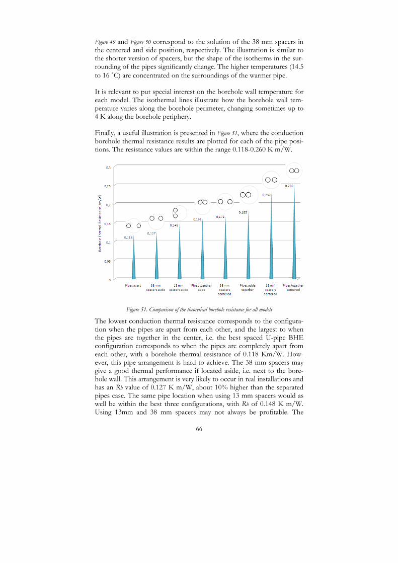
Figure 49 and Figure 50 correspond to the solution of the 38 mm spacers in the centered and side position, respectively. The illustration is similar to the shorter version of spacers, but the shape of the isotherms in the sur-rounding of the pipes significantly change. The higher temperatures (14.5 to 16 ˚C) are concentrated on the surroundings of the warmer pipe.

It is relevant to put special interest on the borehole wall temperature for each model. The isothermal lines illustrate how the borehole wall tem-perature varies along the borehole perimeter, changing sometimes up to 4 K along the borehole periphery.

Finally, a useful illustration is presented in Figure 51, where the conduction borehole thermal resistance results are plotted for each of the pipe posi-tions. The resistance values are within the range 0.118-0.260 K m/W.

Figure 51. Comparison of the theoretical borehole resistance for all models

The lowest conduction thermal resistance corresponds to the configura-tion when the pipes are apart from each other, and the largest to when the pipes are together in the center, i.e. the best spaced U-pipe BHE configuration corresponds to when the pipes are completely apart from each other, with a borehole thermal resistance of 0.118 Km/W. How-ever, this pipe arrangement is hard to achieve. The 38 mm spacers may give a good thermal performance if located aside, i.e. next to the bore-hole wall. This arrangement is very likely to occur in real installations and has an Rb value of 0.127 K m/W, about 10% higher than the separated pipes case. The same pipe location when using 13 mm spacers would as well be within the best three configurations, with Rb of 0.148 K m/W. Using 13mm and 38 mm spacers may not always be profitable. The

66

67

spaced pipes may end up in certain positions that would decrease the thermal performance of the BHE, being even worse than non-spaced configurations. The use of these spacers does not necessarily mean an improvement of the heat transfer performance, but the 38 mm design is likely to result in fairly good thermal performance.

3 . 2 E x p e r i m e n t a l E v a l u a t i o n The experimental work is carried out in a heat pump installation where a building with 19 apartments of 40 m2 each is supplied with domestic hot water and comfort heating by two GSHPs of 16 and 32 kW, respectively. The 16 kW heat pump also supplies comfort heating in case the latter does not have sufficient capacity to cover the building demand. The energy source is six energy wells, a sketch of the installation is found in Figure 55. One of the six borehole heat exchangers (BH4) is the U-pipe tested in chapter 2 (illustrated in Figure 14). Another well (BH5) is the al-ternative U-pipe BHE equipped with the 13 mm spacers that was theo-retically studied in the previous section (illustrated in Figure 40). The first part of the experimental evaluation was done by comparing these two designs through simultaneous distributed temperature measurements. The measurements in both BHEs were always carried out at the same time and same flow during this test, i.e. they had had the same fluid inlet temperature and the same flow rate. However, the measurements always show a slightly lower inlet temperature for the BHE with spacers, prob-ably having to do with the measurement equipment calibration.

Figure 52, Figure 53, and Figure 54 present the fluid distributed temperature profile for both collectors at 0.3, 0.4, and 0.5 l/s, respectively. It can be observed that, in all three cases, the temperature coming from the ground is always at least slightly higher in the U-pipe without spacers, meaning that the thermal performance of this BHE may be somewhat better than the spaced design. The theoretical study from the previous section showed that a spaced U-pipe may sometimes present poorer thermal performance than a U-pipe depending on the pipe positions with respect to each other and to the borehole wall.

The same conclusions drawn in section 2.2 about the heat distribution along the pipe length apply for Figure 52, Figure 53, and Figure 54, i.e. the thermal shunt flow between the down and upward shanks becomes more evident as the flow rate decreases.

Moreover, the two other alternative U-pipe designs: the three pipe col-lector (BH2) and a U-pipe with inner grooves (BH6), have been com-pared through experimental tests. The main characteristics of the four BHE designs are tabulated in Table 6. It is known from chapter 2 that

68

there is not any relevant ground water flow in the surroundings of this installation and that detailed borehole deviation measurements have been carried out every ten meters along their length in order to determine how the borehole diverges from the expected drilling direction. The total ho-rizontal deviation values are also presented in Table 6.

Figure 55 is a sketch of the system including 5 boreholes. The inlet and outlet lines are connected to a common manifold. The volumetric flows are measured in each collector with an inductive instrument of the type Brunata HGS9-R6, the same type of instrument used in chapter 2. Each borehole heat exchanger is instrumented in the secondary fluid side with thermocouples for temperature measurements at the bottom and outlet points. Bottom thermocouples are located about half a meter higher than the collector bottom return line. The inlet temperature is common for all the BHEs and it is measured at a point located before the inlet manifold. All the temperature measurement points are located inside the collector pipes, i.e. the measurement point is in direct contact with the secondary fluid. The total pressure drop in the collectors is also measured during the tests by connecting the instrument TESTO 526-2 to the pressure taps located at the collector inlet and outlet lines.

As it was mentioned before, the secondary fluid used in this installation is an aqueous solution of Ethanol 20% volume concentration, with a freezing point of -8 °C Melinder (2007). All boreholes are water filled and have been working according to the house demand since the system was put in operation. The experiments for this section of the thesis have been carried out during April and May 2008, and the measurement con-dition has been that both heat pumps are on during all tests so that ap-proximately the same energy demand from the boreholes is required. The volumetric flow in the boreholes is adjusted previous to the heat pump start up.

Temperatures have been measured at different flow conditions in the BHEs. As illustrated in chapter 2 (Figure 22), the temperature conditions along the borehole vary with time during short heat extraction periods. In this case, the temperature and the flow measurements are taken every 60 seconds and an average is taken for a 30 minutes long period when the conditions have stabilized after the heat pump start up.

0

20

40

60

80

100

120

140

160

180

200

220

240

260

2 3 4 5 6

Dep

th [

m]

Temperature [˚C]

U-pipe (FO) U-pipe with 13 mm spacers (FO) U-pipe (TC) U-pipe with 13 mm spacers (TC)

Figure 52. Comparison of U-pipe with and without spacers at 0.3 l/s

020406080

100120140160180200220240260

0 1 2 3 4 5 6 7

Dep

th [

m]

Temperature [˚C]

U-pipe (FO) U-pipe with 13mm spacers (FO) U-pipe (TC) U-pipe with 13 mm spacers (TC)

Figure 53. Comparison of U-pipe with and without spacers at 0.4 l/s

0

20

40

60

80

100

120

140

160

180

200

220

240

260

Dep

th [

m]

-2 -1 1 2 3 4 5 6Temperature [˚C]

U-pipe (FO) U-pipe with 13 mm spacers (FO) U-pipe (TC) U-pipe with 13mm spacers (TC)

Figure 54. Comparison of U-pipe with and without spacers at 0.5 l/s

69

Table 6. Description of the BHEs

BHE Active length [m]

Total Horizontal deviation [m] BHE details

2 251.6 84.9 PE 40x3.7mm 3 Pipe collector

4 254.5 64.1 PE 40x2.4mm U-pipe collector

5

242.7

75.7 PE 40x2.4mm

U-pipe with spacers: 13 mm separation between pipes. Separated 2 m from each other at the top 50 meters, and 3 m along the rest of the collector

6 245.7 96.9 PE 40x2.4mm

U-pipe with grooves in helix form. The helix direction is inverted pe-riodically along the BHE length

Figure 55. Sketch of the experimental rig

Each minute, the fluid density, kinematic viscosity and heat capacity are calculated at the measured temperature. The Reynolds number is calcu-lated with equation (9), obtaining the fluid velocity from the measured flow and the pipe inner dimensions. The friction factor is estimated with

70

equation (12) or equation (13), and the pressure drop with equation (11). Finally, the heat absorbed per meter by the secondary fluid is calculated for the down- and upwards flow channel of each collector using equa-tion (14). The latter is immediately used in order to calculate a thermal resistance for down- and upward BHE channels assuming a constant bo-rehole wall temperature and inserting it in the logarithmic mean tempera-ture difference, equation (18). It was shown in theoretical results from section 3.1 that the borehole wall temperature is not constant, meaning that the choice of an appropriate value for these calculations is difficult. This temperature assumption as well as the use of the logarithmic mean temperature difference probably implies a significant uncertainty for the result of this analysis. Moreover, another uncertainty may come with the calculation of a thermal resistance for the down and upward shanks dur-ing a period when the temperature gradients in the borehole change with time. Nevertheless, the analysis is done in order to get some indications about the performance of these borehole heat exchangers.

Figure 56. Groundwater temperature during a heat pump cycle

The rock type at the borehole installation is granite and the undisturbed ground temperature of the site has been carefully measured every one meter along one of the boreholes before the system was put into opera-tion (as presented in Figure 18). The groundwater temperature profile dur-ing heat pump operation has approximately the same shape as the undis-

71

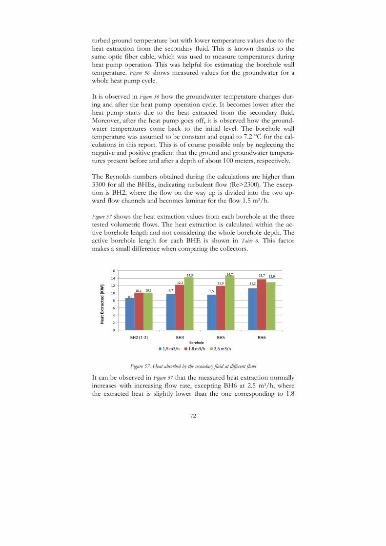
turbed ground temperature but with lower temperature values due to the heat extraction from the secondary fluid. This is known thanks to the same optic fiber cable, which was used to measure temperatures during heat pump operation. This was helpful for estimating the borehole wall temperature. Figure 56 shows measured values for the groundwater for a whole heat pump cycle.

It is observed in Figure 56 how the groundwater temperature changes dur-ing and after the heat pump operation cycle. It becomes lower after the heat pump starts due to the heat extracted from the secondary fluid. Moreover, after the heat pump goes off, it is observed how the ground-water temperatures come back to the initial level. The borehole wall temperature was assumed to be constant and equal to 7.2 °C for the cal-culations in this report. This is of course possible only by neglecting the negative and positive gradient that the ground and groundwater tempera-tures present before and after a depth of about 100 meters, respectively.

The Reynolds numbers obtained during the calculations are higher than 3300 for all the BHEs, indicating turbulent flow (Re>2300). The excep-tion is BH2, where the flow on the way up is divided into the two up-ward flow channels and becomes laminar for the flow 1.5 m3/h.

Figure 57 shows the heat extraction values from each borehole at the three tested volumetric flows. The heat extraction is calculated within the ac-tive borehole length and not considering the whole borehole depth. The active borehole length for each BHE is shown in Table 6. This factor makes a small difference when comparing the collectors.

8,6

9,7 9,5

11,2

10,1

12,2 11,9

13,7

10,1

14,3 14,7 12,9

0

2

4

6

8

10

12

14

16

BH2 (1‐2) BH4 BH5 BH6

Heat E

xtracted

 [KW]

Borehole

1,5 m3/h 1,8 m3/h 2,5 m3/h

Figure 57. Heat absorbed by the secondary fluid at different flows

It can be observed in Figure 57 that the measured heat extraction normally increases with increasing flow rate, excepting BH6 at 2.5 m3/h, where the extracted heat is slightly lower than the one corresponding to 1.8

72

73

m3/h. In BH2 it resulted to be the same. This could be due to the fact that all the measurements were not carried out during the same day, which could alter the borehole temperature conditions. Besides this, the inlet temperature values are not always the same during all the measure-ments and this creates a lower or higher temperature difference between the secondary fluid and the ground, which could have influence on the results. Another factor to mention from Figure 57 is that, at the two lowest volumetric flow rates, the heat extraction is highest in BH6 whilst the lowest in BH2.

It can also be inferred from Figure 57, as shown with the theoretical analy-sis presented above, that the borehole equipped with spacers (BH5) does not give any benefits as compared to the U-pipe (BH4). Their heat ex-traction values are more or less the same. Since the main purpose of this part of the study was to observe the distributed temperature measure-ments in the U-pipe with and without spacers, these two BHEs were al-ways measured at the same time and at the same flow, giving the same inlet temperature when they are measured at each of the volumetric flow rates (as presented earlier in this section).

Figure 58 shows the calculated thermal resistance for the downward and upward channels for the four borehole heat exchangers at the different flows. As previously mentioned, these values are obtained assuming a borehole wall temperature equal to 7.2°C. The first fact reflected in Figure 58 is that the borehole thermal resistance is always higher for the upward channel in the BHEs. This has to do with possible thermal shunt flow, i.e. heat transferred from the upward to the downward channel, as it was illustrated in the results presented in chapter 2. Moreover, the low Rey-nolds numbers obtained in the upward shank of the three pipe BHE at the lowest flow increase the thermal resistance as a consequence of the decrease in the heat transfer coefficient, as presented in equation (21). This situation could change in other unsymmetrical BHEs where the down and upward channels are not equal, as for example the coaxial pipe suggested by Platell (2006).

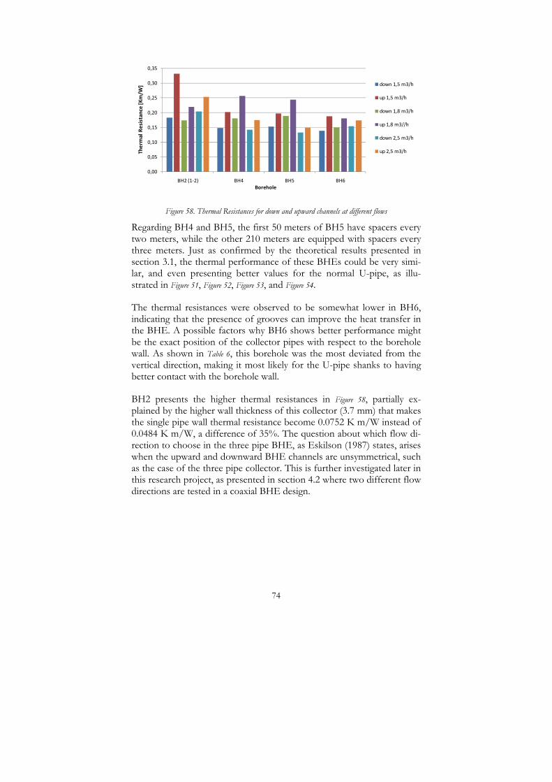
0,00

0,05

0,10

0,15

0,20

0,25

0,30

0,35

BH2 (1‐2) BH4 BH5 BH6

Thermal Resistance [Km/W

]

Borehole

down 1,5 m3/h

up 1,5 m3/h

down 1,8 m3/h

up 1,8 m3//h

down 2,5 m3/h

up 2,5 m3/h

Figure 58. Thermal Resistances for down and upward channels at different flows

Regarding BH4 and BH5, the first 50 meters of BH5 have spacers every two meters, while the other 210 meters are equipped with spacers every three meters. Just as confirmed by the theoretical results presented in section 3.1, the thermal performance of these BHEs could be very simi-lar, and even presenting better values for the normal U-pipe, as illu-strated in Figure 51, Figure 52, Figure 53, and Figure 54.

The thermal resistances were observed to be somewhat lower in BH6, indicating that the presence of grooves can improve the heat transfer in the BHE. A possible factors why BH6 shows better performance might be the exact position of the collector pipes with respect to the borehole wall. As shown in Table 6, this borehole was the most deviated from the vertical direction, making it most likely for the U-pipe shanks to having better contact with the borehole wall.

BH2 presents the higher thermal resistances in Figure 58, partially ex-plained by the higher wall thickness of this collector (3.7 mm) that makes the single pipe wall thermal resistance become 0.0752 K m/W instead of 0.0484 K m/W, a difference of 35%. The question about which flow di-rection to choose in the three pipe BHE, as Eskilson (1987) states, arises when the upward and downward BHE channels are unsymmetrical, such as the case of the three pipe collector. This is further investigated later in this research project, as presented in section 4.2 where two different flow directions are tested in a coaxial BHE design.

74

Figure 59. Pressure drop in BH2 Figure 60. Pressure drop in BH4

Figure 61. Pressure drop in BH5 Figure 62. Pressure drop in BH6

54,2 48,375,0 75,6

144,5129,7

0

20

40

60

80

100

120

140

160

Experimental Calculated

Pressure drop [KPa

]

1,5 m3/h

1,8 m3/h

2,5 m3/h

61,4 56,4

87,378,2

149,6

129,5

0204060

80100120

140160

Experimental Calculated

Pressure drop [KPa

]

1,5 m3/h

1,8 m3/h

2,5 m3/h

56,5 56,7

81,1 78,0

149,6128,4

0

20

40

60

80

100

120

140

160

Experimental Calculated

Pressure drop [KPa

]

1,5 m3/h

1,8 m3/h

2,5 m3/h

49,1 58,070,0 77,3

131,5 136,2

020406080100120140160

Experimental Calculated

Pressure drop [KPa

]

1,5 m3/h

1,8 m3/h

2,5 m3/h

The calculated and experimental values for the pressure drops in the BHEs are plotted in Figure 59, Figure 60, Figure 61 and Figure 62. With the ex-ception of BH6, it is generally observed that the calculated pressure drop is slightly lower than the experimental values. This is attributed to the fact that the accessories such as elbows, bends, bottom part of the col-lector, are not considered in the calculation. The calculated and the expe-rimental pressure drop in BH6 are very similar to each other, meaning that neglecting the grooves roughness may be a good approximation. Moreover, it is observed in Figure 62 that the calculated value is higher than the experimental one, which unexpectedly shows that the real pres-sure drop in this BHE is in fact lower. This alternative U-pipe design presents the lowest pressure drop of all four BHEs, a reason to further study this grooves arrangement.

The difference between the calculated pressure drops for BH4, BH5 and BH6 is attributed to the fact that the flow rates and the temperature le-vels were not always exactly the same in all the tests. Moreover, BH2 presents a pressure drop similar to the other collectors. This would not be expected due to the fact the flow on the way up is divided in two flow channels, reducing the pressure drop on the way up. However, the pipe inner diameter is 32.8 mm and not 35.2 mm as for the other alternative designs, causing the opposite effect over the pressure drop.

75

4 Experiences with Coaxial BHEs

Different borehole heat exchanger designs have been tested and dis-cussed in the previous chapters of this thesis. They are all based on the U-pipe BHE principle that has been used for several years. Given the in-creased interest on innovation within this field during the work on this thesis, this chapter presents the first measurement results from two coaxial BHE prototypes, both having a particular geometry. The first one consists of an inner central pipe with an annular flow channel in close contact with the borehole wall, and the second consists of one central pipe with five trapezoidal external channels.

In section 4.1, the annular design is described and fluid temperature measurements taken every ten meters along the borehole depth during a distributed thermal response test are shown and discussed. A measure-ment of the borehole wall temperature illustrates the heat transfer per-formance potential of the annular flow channel.

In section 4.2, the particular geometry of the other coaxial prototype is thermally analyzed in 2D with a finite element calculation similar to the one carried out in chapter 3. This is followed by an experimental evalua-tion consisting of two in situ thermal response tests. Measurements of the pressure drop at different flow rates are also presented.

4 . 1 A n A n n u l a r C o a x i a l B H E - f i r s t p r o t o t y p e

The borehole heat exchanger is 189 meter long. A cross section showing the dimensions and a longitudinal view of this BHE are presented in Figure 63 and Figure 64, respectively. It can be observed that it consists of a central pipe and an annular external channel in contact with the borehole wall.

Figure 63. Cross section of the annular coaxial BHE

76

The idea with this design is to decrease the physical distance between the secondary fluid and the rock by means of the annular channel that is ex-ternally delimited by a thin hose (0.4 mm thick) in close contact to the borehole wall, as illustrated with the green color in Figure 63 and Figure 64.

The thin hose, normally called energy capsule (PEMTEC AB), is the first part that is installed into the energy well. The installation procedure is simple: it is sent into the well and subsequently filled with water.

Figure 64. Longitudinal sketch of the coaxial BHE

Figure 65. Energy capsule before water fill-ing.

Figure 66. Bottom part of energy cap-sule with external fiber optic cable

Figure 67. Central pipe, internal bottom weight and fiber cable

The borehole diameter is 115 mm and the energy capsule is delivered with a diameter of 114 mm, among others. Once the capsule is filled with water, it seals the borehole from the surrounding rock and ground-water. Originally, the energy capsule was thought to be used in energy wells for groundwater protection from possible leakage in the BHE pipes.

The installation of this coaxial BHE has allowed installing a fiber optic cable between the energy capsule and the rock, thereby making it possi-

77

78

ble to estimate the borehole wall temperature. A slightly higher pressure in the inner part of the capsule tightens the fiber against the borehole wall. The location of this fiber optic cable is illustrated in Figure 64, Figure 65, and Figure 66.

Figure 66 and Figure 67 show the first moment of the installation. The energy capsule and the external fiber optic cables are first installed into the bo-rehole with the help of a bottom weight. This process took approximate-ly 20 minutes. Figure 65 shows the energy well after this moment was completed, where it can be observed that the energy capsule is still flat, meaning that it has not yet been filled with water. The duration of the water filling process depends on the borehole dimensions, the injection flow rate, and of the presence of higher groundwater pressures at a cer-tain depth that may slow down the capability of water to fill the capsule. Once the energy capsule is filled with water, the installation of the central channel constitutes the next step, just as a normal BHE installation.

The central channel is, in this case, a typical polyethylene tube for GSHP installations of the type PE 40x2.4 mm. Figure 67 presents the channel to-gether with a bottom weight. The latter is used to facilitate the pipe in-stallation. A high degree of eccentricity is expected since no centralizers have been used. Visualizations with an underwater camera have con-firmed that the pipe is not centered. It is worth mentioning here that this is the first of a series of tests where several central pipes will be tested in similar arrangements in order to evaluate the benefits of, for example, in-sulation of the central flow channel.

The capsule and the central pipe were easily inserted as when inserting common U-pipe BHEs, although the fiber optic cables made the installa-tion work more special. In other words, the installation process of such BHE does not have any complications. An exception could be areas with loose soils, high groundwater flow or cracks, which may set hurdles when installing the energy capsule. Experiences from other coaxial BHE designs as the ones described in section 1.6 point out complications dur-ing the installation process due to buoyancy forces and BHE stiffness when rolling it out from the delivery package, a problem that practically disappears in this particular prototype design. However, such problems may arise if the central pipe is to have better insulation characteristics.

Since low temperature differences between the borehole wall and the cir-culating fluid are expected, the initial idea is to use water as a circulating fluid, instead of an antifreeze aqueous solution, offering significant ad-vantages from the hydraulic, thermal and environmental point of view. There is, however, a risk for fluid freezing in cold places where the un-disturbed ground temperature is close to the water freezing point condi-

tions. This will principally be determined by the lowest temperature in the heat pump evaporator.

The measurements with fiber optics in the groundwater side presented in Figure 21 and Figure 56 show a wide spread of temperature values due to the unknown exact location of the cable in the borehole. This problem is partially solved with this installation, thanks to this fiber that has been tightened against the borehole wall. Moreover, a second cable located in-side the flow channels is used for measuring the secondary fluid temper-ature. The optical fiber cables used in this test are also of type 50/125, with two graded index multimode fibers coated with a thin stainless steel tube. The fiber cable diameter is 3.8 mm.

A distributed thermal response test was carried out in this prototype, measuring temperatures every 10 meters along the well. This test has been done using water as secondary fluid and the measurements are tak-en in the water side along the downward and upward channels, accom-panied by the measurement of the borehole wall temperature. The tem-perature readout equipment is of type HALO-DTS and the measure-ment integration time is of 5 minutes. A constant heat injection rate has been applied during about two days. The average temperature profile along the borehole depth during the whole heat injection period is illu-strated in Figure 68, also showing the borehole wall temperature.

10

30

50

70

90

110

130

150

170

190

12 13 14 15 16

Dep

th [m

]

Temperature [°C]

upwards downwards Borehole wall

Figure 68. Average temperature profiles in coaxial BHE

The average injection temperature is about 15.5°C. The temperature at the bottom is 14°C and the outlet temperature is 12.6°C. A significant portion (about 50%) of the heat is transferred when the fluid travels

79

80

through the central pipe. The rest of the heat is transferred in the annular channel. It is observed how the borehole wall temperature profile fol-lows almost perfectly the shape of the annular flow, differing by about 0.4°C. A slight asymptotic tendency is observed at the last 40 meters of the upward flow, meaning that significant thermal shunt flow starts to take place.

Trusting the borehole wall temperature measurement, an estimation of Rb along the borehole length can be done from Figure 68 after calculating the specific heat injection. This will be carefully done and confirmed with a complete Distributed Thermal Response Test analysis in the con-tinuation of this study.

A contribution of the gap resistance could probably emerge due to the fact that the BHE worked almost as an open system with slightly low pressure difference between the inner and outer part of the capsule. The groundwater level outside the energy capsule is 3 m under the ground surface and a three meters water column above this level was kept con-stant in the inner part during the test for guaranteeing the cylindrical at-tachment of the capsule to the borehole wall.

The low temperature difference between the fluid flowing through the annular channel and the borehole wall points at several potentials for improvements of this BHE design, as for example insulating several me-ters or increasing the thickness of the central pipe.

4 . 2 C o a x i a l p r o t o t y p e w i t h f i v e e x t e r n a l f l o w c h a n n e l s

The Borehole Heat Exchanger evaluated here is a coaxial prototype con-sisting of one central pipe and five external channels of trapezoidal cross section, as illustrated in Figure 69. The external channels are connected in parallel with each other and in series with the central channel. Figure 70 is a view from above of the well after the BHE was successfully installed. More details of the design as well as some simulation results from this BHE are found in the work by Andersson (2008).

The idea behind this BHE design is to have a single pipe package, the ex-ternal channels of which are located close to the borehole wall and that is delivered in the same way as today’s U-pipe BHEs, in a roll that is un-coiled as the pipe is inserted into the borehole.

The well, where this prototype is installed, is water filled, has a depth of 260 m and a diameter of 140 mm. It is located at the same installation as all the BHEs tested in chapter 2 and 3. In this well, the groundwater

level oscillates around 13 m below the ground surface. The fluid used is also an aqueous solution of Ethanol at 20% volume concentration. It has operated for about one year at the moment when these tests were carried out. The average undisturbed ground temperature in the installation is 9.1°C, according to the measurements from an adjacent well presented in chapter 2.

Figure 69. Cross section of

the coaxial BHE

Figure 70. View of the BHE after installation

The prototype is instrumented with two inductive flow meters of the type Brunata HGS9-R6, two Pt 500 resistance thermometers for meas-urement of the inlet and outlet fluid temperatures into the borehole, a STA-D regulation valve, and an extra temperature measurement point (T type stainless steel sheathed thermocouple) at the borehole bottom. The latter is inserted on the brine side of one of the outer channels and con-nected through a thermocouple cable and a temperature reference box (which contains the reference junction in a constant temperature block and a Pt-100 sensor) to an Agilent data acquisition unit. The thermocou-ple was preheated and inserted through the pipe wall as illustrated in Figure 71. The insertion point was protected with a shrinking hose as shown in Figure 72.

Figure 71. Insertion of the bottom thermocouple

Figure 72. Protection of the bottom thermocouple with shrinking hose

In order to evaluate the performance of this coaxial BHE prototype, two in situ thermal response tests and a 2-D steady state simulation have been carried out. In addition, the pressure drop was measured at four different flow rates and compared with the pressure drops at the corres-ponding flows in a U-pipe BHE.

81

82

The two thermal response tests are denoted as TRT1 and TRT2. The distinction between these tests is that the fluid is circulated in two differ-ent flow directions, i.e. flowing downwards through the central pipe and upwards through the outer channels during TRT1, and vice versa during TRT2. The flow rate was continuously measured in order to ensure that it was the same during both tests.

The fluid temperature has been measured in all three measurement points, i.e. at the inlet, bottom and outlet of the BHE. The measure-ments are done during two continuous phases, pre-circulation and heat injection, lasting about 27 and 48 hours, respectively. The pre-circulation phase of the test estimates the ground temperature before starting the heat injection. Subsequently, a reasonably constant heating power of ap-proximately 10 kW has been supplied to the BHE during the heat injec-tion period of both tests. This power has been chosen considering that the active borehole length is 236 m, which gives a specific heat rate of 42.3 W/m borehole, a typical standard design heat rate for a ground source heat pump application. The borehole daily operation (heat extrac-tion activities) was closed one week before TRT1 was started. TRT2 started 17 days after TRT1 was finished, and the borehole was not in op-eration during this interim period. The analysis of TRT2 accounts for the power supplied during TRT1. The results of both in situ tests give a measure of the undisturbed ground temperature, the average thermal conductivity of the rock (λrock), and the effective borehole thermal resis-tance (Rb) for each test.

Furthermore, given the undisturbed ground temperature obtained from the TRT, a cross section (2-D) of the 140 mm borehole with the coaxial BHE has been modeled using the finite element method software COMSOL Multiphysics, and only considering heat transfer by conduc-tion. A rock diameter of one meter around the borehole has been chosen as the outer reference boundary. The temperature at the inner wall of each flow channel has been used as boundary condition (equal to a mean temperature along the central and the outer channels obtained from a certain moment during TRT2). This is done by averaging the inlet and bottom temperature for the downward flow, and the bottom and outlet temperature for the upward flow. Thus, there are two independent tem-perature differences between the fluid and the undisturbed rock, and two independent heat flows. The total net heat flow q’ to the outer circle is the algebraic sum of the ones corresponding to each of them. This alge-braic sum accounts for the heat flow between the center pipe and the pe-ripheral channels.

The convective heat transfer inside all the flow channels is modeled by introducing a previously calculated heat transfer coefficient as a boun-

83

dary condition at their internal wall based on equation (16). The fluid flow rate is 0.7 l/s, as during the TRTs. The Reynolds number in the central pipe for TRT1 and TRT2 is 10817 and 9791, respectively. The corresponding Re for the outer channels was 3382 for TRT1 and 3460 for TRT2 (the values of TRT2 are used for the simulation). The thermal properties of the fluid are obtained from Melinder (2007) at the mean temperatures. All the Internal flow boundary conditions are tabulated in Table 7.

Table 7. Internal flow boundary conditions

Heat transfer coefficient central [W/m2K] 1102 Heat transfer coefficient outer channels [W/m2K] 940 Temperature central channel [°C] 15.2 Temperature outer channel [°C] 17.0

COMSOL Multi-physics, has been used in order to quantify the net heat flow from the BHE channels to the rock by a steady state conduction heat transfer analysis. These heat flows are then used to calculate the fluid to ground thermal resistance (RT), and subsequently a borehole re-sistance for pure conduction heat transfer. In this case, the borehole thermal resistance is denoted as Rcond in order to differ it from the one obtained in the TRTs. Rcond is calculated just as in the theoretical analysis presented in section 3.1, by subtracting the contribution of the surround-ing rock (Rrock) from RT with equation (19), assuming Rb = Rcond. The cal-culation of Rrock is based on the λrock obtained from the TRT using equa-tion (20), and RT is obtained dividing the temperature difference between the average fluid (a mean of the values given in Table 7) and the rock tem-perature set as a boundary condition at the outer border of the rock. The natural convection between the BHE pipes and the borehole wall has again been neglected in this theoretical study.

The thermal properties of the PE pipes were taken from (Basell) and the ones corresponding to the rock (granite) are based on Eriksson (1985), except the thermal conductivity that was obtained from the TRTs. These characteristics are presented in Table 8.

Table 8. Some thermo physical material properties

Rock Density [kg/m3] 2700 Specific Heat Capacity [J/kg K] 830

Polyethylene pipes PE Density [kg/m3] 950 Specific Heat Capacity [J/kg K] 2000 Thermal conductivity [W/m K] 0.4

The pressure drop has been measured as in the experiments from section 3.2, by connecting a TESTO 526-2 instrument between two pressure taps located at the collector inlet and outlet lines (the fluid temperature levels during these measurements do not correspond to the ones during the TRTs). These have been done at four different flow rates: 0.3, 0.4, 0.5, and 0.7 l/s and the results are compared with the ones from a U-pipe BHE of approximately the same length.

Figure 73 shows the thermal power supplied to the fluid and the volumetric flow rate along the heat injection phase of both thermal response tests. A step in flow and power is observed sometime before 30 hours have passed, indicating the start of the heat injection phase. Since then, it is observed that the flow is held relatively constant at about 2550 l/h (0.71 l/s) and that the supplied heat was about 10 kW during both TRTs.

Figure 73. Supplied power and flow rate during both TRTs

A slight increase of the flow develops as the fluid becomes warmer. Its viscosity and density decrease, allowing a flow increase for the same pressure drop. The supplied heat oscillated around 10 kW during both TRTs. These variations are accounted for during the TRT analysis by considering the temperature response due to step changes in the sup-plied power and superposing it to the temperature change contributions at all previous time steps.

Figure 74 shows the temperature variation during the pre-circulation and the heat injection phases of both tests. Tin, Tout and Tbottom stand for inlet, outlet, and bottom temperatures, respectively. During pre-circulation, the mean fluid temperature Trock = Tf (average between Tin and Tout) was 8.40°C for TRT1 and 8.79°C for TRT2, meaning that the average ground temperature at the moment when these pre-circulation phases were carried out is lower than the one measured at the adjacent borehole some months earlier (9.1°C as mentioned in chapter 3). There exists a

84

small heat recovery effect behind these measurements (including the ef-fect of TRT1 over TRT2) that may influence the TRT results and must be considered, adding some degree of uncertainty to the determination of λrock and Rb.

Figure 74. Measured temperatures during TRT1 and TRT2

In order to correct for this, a temperature slope term was added to the undisturbed temperature measurements along the whole duration of both tests. This was done given that the evaluation of TRT2 can be car-ried out considering the pre-circulation and heat injection phases of TRT1, i.e. the effect of TRT1 over TRT2 can be easily calculated with equation (25) accounting for the whole time period of and between TRT1 and TRT2. Hence, it is possible to estimate a slope value that, when used in the analysis of TRT2 with 8.40°C as a starting point for the ground temperature, produces the same results as for the calculation of TRT2 without the influence of TRT1 with 8.79°C as undisturbed tem-perature. Such estimation resulted in a slope of 0.0006 K/h.

During the heat injection phase, it is observed in Figure 74 that the inlet and outlet temperatures are nearly the same during both TRTs, where the total temperature change in the BHE (Tin-Tout) is about 3.5°C. For a given power supply and volumetric flow rate, it is logical that the total temperature change is independent of the flow direction. However, the temperature distribution along the downwards and upwards flow chan-nels changes significantly with the flow direction. This is evidenced by the temperature measurements at the bottom point.

It is clear in Figure 74 that the measured bottom temperature is about 2°C higher during TRT1 than TRT2. During TRT1, the fluid temperature decreases along the flow direction, i.e. Tin > Tbottom > Tout, whilst for TRT2, the temperature drastically increases between Tbottom and Tout, an evidence of the large thermal contact between the central pipe and the

85

outer channels. A higher volumetric flow rate would improve this situa-tion by decreasing the temperature difference between the up- and downward flows in the BHE.

(a)

(b) Figure 75. Temperatures during optimization of both TRTs

During a 30 hour period, between 40 and 70 hours of the heat injection phase of both tests, the temperature difference between the fluid and the undisturbed ground as a function of time has been calculated with equa-tion (25) and a program that subsequently minimizes the squared errors between the calculated and the measured temperatures, in order to make the best approximation to the measurements. The results of this optimi-zation are illustrated in Figure 75(a) for TRT1 and Figure 75(b) for TRT2. It can be observed that the measured and the calculated values follow the same track along the whole minimization period regardless of the tem-perature fluctuations that in part are due to the fluctuations in heat sup-ply. The main results of both TRTs, the thermal performance of the BHE (Rb) and the thermal conductivity of the rock (λrock), are presented in Table 9.

86

87

Table 9. TRT results from the infinite line source model

Test TRT1 TRT2 krock [W/m K] 3.30 3.24 Rb [K m/W] 0.096 0.094

As expected, the borehole thermal resistance and the rock’s thermal conductivity were almost the same for both tests. As shown in chapter 2, a previous TRT carried out in the adjacent borehole resulted in a rock thermal conductivity of 3.1 W/m K. This slight variation could be due to small changes in the rock thermal properties or to a possible groundwa-ter flow in the borehole.

Regarding Rb, it is shown in Table 9 that the outcome was in average about 0.095 K m/W, a number that is slightly higher than the one obtained for U-pipe BHEs. The influence of the previous activity in the borehole may change this value by some extent. However, this result is an indication that the thermal performance of this coaxial prototype is very similar to the one corresponding to a U-pipe design. This is exemplified with the results from the 2-D heat conduction simulation as follows below.

Figure 76 shows a visualization of the temperature contour around the co-axial BHE for two different positions in the borehole after modelling and simulating a cross section of this design: (a) the BHE is concentric; (b) the BHE is eccentric and close to the borehole wall. Besides tempera-ture, Figure 76 also illustrates the heat flux direction through heat flux ar-rows.

It can be observed in Figure 76(a) that, as expected, the temperature distri-bution in the borehole is symmetric. A better contact with the ground is achieved when the BHE is eccentric since higher temperatures outside the borehole are obtained. In view of the fact that the thermal conduc-tivity of the rock is not the same as in the water, the temperature distri-bution in this case is asymmetric. In both cases, Figure 76(a) and (b), the warmest part of the cross section is located at the lateral walls of the outer channels, which is caused by the relatively small heat flow through them. One of the ideas behind this design is to maximize the heat trans-fer area in the outer channels, but the lateral walls seem to have a small influence over this design premise, at least when only conductive heat transfer is considered. This scenario may change when convection on the groundwater side is taken into account in the analysis. Of particular in-terest from these results is, once again, the thermal contact between the central and the outer channels, illustrated by the heat flux arrows. The heat flowing between these is inversely proportional to the wall thickness between them, meaning that it is of preference to increase the insulation

effect of this pipe and to narrow the contact area in order to achieve lower thermal shunt flow between the down- and upward fluid flows.

(a)

(b) Figure 76. Cross section temperature contour

and heat flux arrows

The result of calculating the conduction borehole thermal resistance Rcond from this simulation becomes 0.18 K m/W for the case when the BHE is centered, and 0.15 K m/W when it is located aside. An illustration of this is shown in Figure 77, where the result is also compared with the one corresponding to a similar simulation of a U-pipe BHE. The borehole thermal resistance Rcond for the coaxial BHE prototype is, as for the in situ test result, of about the same magnitude as for the U-pipe. The simulations for the U-pipe positions are according to the results pre-sented in section 3.1.

Regarding the pressure drop measurements, Figure 78 shows a experimen-tal comparison between the coaxial prototype and a U-pipe BHE at four different volumetric flow rates. It is observed that, at all four flow rates, the pressure drop in this coaxial prototype is significantly lower than in a U-pipe (about 65% difference), representing an advantage due to the fact that the necessary pumping power may not be as high for the coaxial BHE design. However, the pumping power is also approximately pro-portional to the cube of the flow rate, which for this coaxial design and this borehole depth, should be higher. It was observed from the thermal response test results that 0.7 l/s is probably not the optimum volumetric

88

flow rate for this borehole depth, as the thermal shunt flow between channels manifests. If the flow rate had been increased, the borehole thermal resistance would have been reduced, perhaps to a lower value than for a U-pipe BHE.

Figure 77. Theoretical conductive thermal resistance of coaxial and U-pipe

Figure 78. Pressure drop in coaxial BHE prototype and U-pipe BHE at four flows

89

90

5 Conclusions

Experimental work has been carried out in different ground source heat pump installations where energy is exchanged with the ground in differ-ent borehole heat exchanger designs.

The undisturbed ground temperature profile in most of the installations has a negative gradient at the shallowest depths, but later present a tem-perature increases with a positive gradient of about 1K/100 m.

One BHE has been characterized in detail including measurements of its deviation along the depth. It resulted to be deviated 56.4 m and 30.5 m towards east and north from the vertical direction, respectively. Similar values were measured for the other boreholes of the installation. Moreo-ver, differential groundwater flow measurements identified that no sig-nificant ground water flow takes place in this borehole. It was registered to be approximately 0.4 l/min along the whole length and no local ef-fects due to groundwater flow differences along the borehole length are detected. However, a slight anomaly was found in the interval between 180 and 200 m depth.

Temperature measurements with optic fiber cables and thermocouples have been done in the secondary fluid and groundwater side in two U-pipe BHEs, one common design and one alternative design with 13 mm spacers between pipes, providing a detailed picture of typical tempera-ture profiles, the profile behavior in time, and at different fluid flow rates. The correspondence between the temperature measurements with optic fiber cables and thermocouples varies between 0°C and 0.7 °C, at-tributed to differences in the measurement principle and to possible con-trast between the flow regime and the location of the measurement point. The measurements have been done at three different flow rates: 0.3 l/s, 0.4 l/s, and 0.5 l/s; aiming at the evaluation of the effect of the secondary fluid flow rate and the relative distribution of the specific heat extraction along the borehole depth. They resulted in evident thermal contact between U-pipe channels, increasing with decreasing flow rates. The distribution of the heat extracted along the down and up-going pipes becomes more equal as the mass flow increases.

91

In order to have a clear picture of flow regime transitions in U-pipe BHEs, pressure drop measurements along a horizontal pipe where an aqueous solution of Propylene glycol with 32% weight concentration (-14°C freezing point) is circulated at different flows have been done. For-ty pressure tabs for pressure measurements are located along a U-pipe BHE with 5 meters distance between them. The tendency of the pres-sure drop slopes before and after the U-pipe bend for each of the volu-metric flows is the same for both sections, meaning that the flow regime behaviour tends to be the same before and after the bend. A slightly lar-ger pressure drop in the U-pipe bend, remarks the importance of follow-ing the welding standards for the bottom part BHEs. Practical experi-ences during this research have shown that the cross section of the pipe may be drastically reduced depending on the welding quality. The total pressure drop in the loop may be affected by this. This situation changes from pipe to pipe, and from manufacturer to manufacturer.

A comparison between the experimental and theoretical pressure drop for this installation shows that the experimental values are in good ac-cordance with the theory in all cases.

Besides the U-pipe with spacers, two other alternative U-pipe borehole heat exchangers have been tested. All alternatives are products donated by the project sponsors and they include: two type of spacers to ensure the separation of the U-pipe shanks (13 and 38 mm between pipes) along the depth and guarantee their proximity to the borehole wall, grooves in the U-pipe inner wall, and a third pipe added to the U-pipe BHE, nor-mally called three pipe BHE. The thermal resistance for the upward channel in all designs was always higher than for the downwards flow channel in all BHEs. This has to do with possible thermal shunt flow, i.e. heat transferred from the upward to the downward channel.

Distributed temperature measurements in the U-pipe with 13 mm space-rs and without spacers, always measured at the same time and at the same flow, showed that these spacers do not give any benefits as com-pared to the U-pipe. Their heat extraction, temperature profiles, and thermal resistances values are more or less the same. However, theoreti-cal calculations show that 38 mm spacers may represent a better alterna-tive for improvements of the U-pipe design in a 140 mm borehole.

Low Reynolds numbers obtained in the upward shank of the three pipe BHE at low fluid volumetric flow rates increased the thermal resistance as a consequence of the decrease in the heat transfer coefficient. Moreo-ver, the high thermal resistances are partially explained by the higher wall thickness of this collector (3.7 mm) that makes the single pipe wall ther-

92

mal resistance become 0.0752 K m/W instead of 0.0484 K m/W as for standard U-pipes.

The thermal resistance and the measured pressure drop were observed to be somewhat lower in U-pipe with grooves in the inner wall of the BHE pipes. It should be noted that the better thermal performance may also be caused the fact that this borehole was the one deviating most from the vertical direction, making it likely for the U-pipe shanks to having better contact with the borehole wall.

In groundwater filled boreholes, it is common to expect certain degree of natural convection outside U-pipe BHEs, resulting in lower borehole thermal resistances, especially during heat injection thermal response tests. Neglecting this phenomenon, a simple steady-state heat conduction analysis of U-pipe BHEs was carried out in a borehole with diameter 140 mm equipped with two spacer dimensions, indicating that Rb varies be-tween 0.11 – 0.26 K m/W for the best and worst pipe positioning, re-spectively (using PE 40x2.4mm pipes). Thermal Response Testing of U-pipes normally results in values between 0.06-0.08 K m/W depending on how much natural convection takes place during the test and on the bo-rehole dimensions. In this theoretical evaluation, the lowest borehole re-sistance was obtained for a configuration when the pipes are apart from each other, and the largest value when the pipes are together in the cen-ter. The 38 mm spacers may give a good thermal performance if located aside, i.e. next to the borehole wall. This arrangement is very likely to oc-cur in real installations and has a conduction borehole thermal resistance of 0.127 K m/W. The same pipe location when using 13 mm spacers would as well be within the best three configurations, having 0.148 K m/W. Using the 13 mm spacers may not be profitable in 140 mm bore-holes. The spaced pipes may end up in certain positions that would dete-riorate the thermal performance of the BHE.

The rock thermal conductivity and borehole thermal resistance were de-termined in 12 different sections along the depth of a U-pipe BHE dur-ing a Distributed Thermal Response Test (DTRT). The surrounding rock appears to be relatively homogeneous with an average value of 3.10 W/m K, showing good agreement with the result from a conventional TRT analysis. The borehole resistance variations along the depth had an average of 0.062 K m/W, differing within the range 0.054 – 0.068 K m/W and indicating that the relative pipe position may change in the bo-rehole.

During this DTRT, the mean ground temperature was measured in a U-pipe BHE during zero flow conditions and pre-circulation of the work-ing fluid during a distributed thermal response test. The result validates

93

previous studies regarding the influence of pumping power on the as-sessment of undisturbed ground temperature during TRTs.

The average borehole thermal resistance remarkably disagrees with the result from conventional TRT analysis (0.079 K m/W), mainly attributed to the use of a less accurate fluid mean temperature during standard TRTs.

The interest for designing cost effective BHEs characterized by mod-erate temperature differences between the secondary fluid and the sur-rounding ground, and easiness during installation have resulted in sug-gesting and installing a novel coaxial borehole heat exchanger, consisting of an inner central pipe and an annular channel in close contact with the borehole wall. The installation procedure was simple, as rapid as when inserting common U-pipe BHEs.

This first evaluation of this coaxial design includes a distributed thermal response test with similar heat injection rates as for standard U-pipes. The measurements were done using fiber optic cables that measured the circulating fluid temperature every 10 meters during circa 2 days, show-ing that about 50% of the heat is transferred when the fluid travels through the central pipe. The high temperature difference between the down and upward flows negatively affects the average fluid temperature, especially at lower depths. This will result in an increased borehole resis-tance value for this particular case. A measurement is also done with a optic fiber cable tightened between the rock and the annular channel. It is clearly observed how the borehole wall temperature profile follows the shape of the annular flow, differing by about 0.4°C.

A hypothetical advantage of this BHE is that it might be possible to use water as a secondary fluid, resulting in benefits from the thermal, hydrau-lic and environmental point of view. Future work will consist of carrying out a complete distributed thermal response test and testing different central pipe alternatives.

Finally, a study of a prototype coaxial borehole heat exchanger consisting of one central pipe and five trapezoidal external channels has been pre-sented. The study consisted of a 2-D steady state conduction analysis with the FEM software COMSOL Multiphysics and a experimental eval-uation by two in situ thermal response tests. The latter was carried out with two different flow directions and an extra temperature measure-ment point at the borehole bottom that illustrated the heat distribution along the heat exchanger for the different flow direction options. The to-tal pressure drop has also been measured at four different flow rates.

94

The supplied power during the in situ tests oscillated around 10 kW and its variations were accounted for by considering the temperature re-sponse due to step changes in the supplied power and superposing it to the temperature change contributions at all previous time steps.

The influence of previous heat extraction activities in the borehole was evidenced by an average ground temperature measured during the pre-circulation phase of the TRTs of 8.4°C for TRT1 and 8.79°C for TRT2, which is lower than the observed 9.1°C for the undisturbed rock in the adjacent borehole. A slope term was added to the undisturbed ground temperature along the whole duration of both tests in order to correct for this.

During the heat injection phases of the in situ tests, the average tempera-ture difference between the fluid and the rock was almost the same. However, the temperature distribution along the downwards and up-wards flow channels significantly changed with the flow direction. This was shown by the bottom temperature measurement point being over 2°C higher during TRT1 than TRT2. Significant thermal contact be-tween the central pipe and the outer channels was identified here as well as during the FEM simulation.

For the FEM simulation, two cross sectional configurations were mod-eled, calculated, and compared with each other and with the U-pipe de-sign. The boundary conditions were based on the TRT experimental temperature measurements and calculated heat transfer coefficients. The two-dimensional problem was solved with the steady state heat transfer equation. The borehole thermal resistance was calculated in order to quantitatively compare the thermal performance of the presented cases. A temperature contour plot and heat flow directions illustrate how heat is transferred between the rock and the pipes as well as the thermal shunt flow occurring between channels. Almost no heat passed through the lateral walls of the outer channels.

The outcome of calculating the borehole thermal resistance from the in situ tests and the simulation was a value within the same range as for U-pipe borehole heat exchangers, meaning that the thermal performance of these two designs is similar and that improvements on the coaxial proto-type are necessary. A straightforward potential for enhancement is the increase of the central pipe thickness and the use of higher volumetric flow rates.

The pressure drop in the coaxial prototype was, at all flow rates, about 65% lower than in a U-pipe.

95

6 References

Acuña, J. (2008). Characterization and Temperature Measurement Techniques of Energy Wells for Heat Pumps. Master of Science Thesis Energy Technology 2008:450. Stockholm: KTH.

Andersson, J. (2008). Geothermal Energy Study. Åbo: Åbo Akademi University, Faculty of Technology.

Basell. Technical Manual for Pipe Materials - Polyethylene. Hostalen, Lupolen.

Bose, J. M. (2002). Advances in Ground Source Heat Pump Systems - An International Overview. 7th IEA Heat Pump Conference. 1:313-324. Beijing.

Claesson J, B. J. (1987). Multipole method to compute the conductive heat flows to and between pipes in a cylinder. Dept. of Building Technology and Mathematical Physics.

Claesson J, E. B. (1985). MARKVÄRME - En handbok om termiska analyser. Lund: Avd. för Matematisk fysik och Byggnadsteknik, LTH.

Claesson J, E. P. (1988). Conductive Heat Extraction to a Deep Borehole: Thermal Analyses and Dimensioning Rules. Energy vol. 13, no. 6 , 509-527.

Claesson J, E. P. (1988). Conductive heat extraction to a deep borehole: Thermal Analyses and Dimensioning Rules. Energy 13(6) , 509-527.

Eklöf C, G. S. (1996). TED - A Mobile Equipment for Thermal Response Test. Luleå: Luleå University of Technology.

Eriksson. (1985). Värmeutbyte mellan berggrund och borrhål vid bergvärmesystem. Gothenburg: Chalmers University of Technology and University of Göteborg.

Esen H, I. M. (2009). Temperature distributions in boreholes of a vertical ground-coupled heat pump. Renewable Energy , 2672-2679.

96

Eskilson P, H. G. (1987). Response Test for a Heat Store with 25 Boreholes. University of Lund, Mathematical Physics and Building Technology. Lund: Notes on Heat Transfer 9-1987.

Eskilson, P. (1987). Thermal Analyses of Heat Extraction Boreholes. Lund, Sweden: Department of Mathematical Physics, Lund Institute of Technology.

EWS. (2006). GROUNDHIT - brief report on deliverable No. 8 - Design drafts - description of pre-prototype borehole heat exchanger. Lichtenau: Erdwärme-Systemtechnik GmbH & Co. KG.

Farhadiroushan, M. (2009). Personal communication.

Fuijii Hikari, O. H. (2006). Thermal Response Tests Using Optical Fiber Thermometers. GRC Transactions, 2006. - Vol. 30. , Kyushu University, Fukuoka.

Gehlin Signhild. (2002). Thermal Response Test - Method, Development and Evaluation [Doctoral Thesis]. Luleå: Luleå University of Technology.

Gehlin Singhild, N. B. (2003). Determining Undisturbed Ground Temperature for Thermal Response Test. ASHRAE , Vol. 109, Pt.1.

Gehlin, S. (2002). Thermal Response Test - Method, Development and Evaluation. Luleå: Luleå University of Technology.

Gnielinski, V. (1976). New equations for heat and mass transfer in turbulent pipe and channel flows. Int. Chem. Eng. 16 , 359-368.

Gustafsson A-M, W. L. (2010). CFD-modelling of natural convection in a groundwater-filled borehole heat exchanger. Applied Thermal Engineering 30 , 683-691.

Gustafsson, A. (2006). Thermal response test: numerical simulations and analyses. Luleå: Licenciate Thesis LTH 2006:14.

Hellström G, K. E. (2000). Laboratory measurements of heat transfer properties of different types of borehole heat exchangers. Proc. of Terrastock , August 28 – September 1, 2000. Stuttgart, Germany.

Hellström, G. (2002). Borehole Heat Exchangers - State of the art. Lund: IEA.

Hellström, G. (1991). GROUND HEAT STORAGE, Thermal Analyses of Duct Storage Systems [Doctoral Thesis]. Lund: LTH.

97

Hellström, G. (1998). Thermal Performance of Borehole Heat Exchangers. The Second Stockton International Geothermal Conference.

Incropera F, D. D. (2007). Fundamentals of Heat and Mass Transfer. NJ: John Wiley & Sons.

Ingersoll L.R, P. H. (1948). Theory of the Ground Pipe Heat Source for the Heat Pump. ASHVE Transactions , Vol. 54.

Johan Claesson, B. E. (1985). Markvärme - En handbok om termiska analyser. Lund: Avd för Matematisk fysik och byggnadsteknik LTH.

Melinder, Å. (2007). Thermophysical Properties of Aqueous Solutions Used as Secondary Working Fluids [Doctoral Thesis]. Stockholm: The Royal Institute of Technology KTH.

Mogensen, P. (1983). Fluid to Duct Wall Heat Transfer in Duct System Heat Storages. The International Conference on Subsurface Heat Storage in Theory and Practice, (ss. [Appendix, Part. II, p. 652-657]). Stockholm.

Platell, P. (2006). Developing Work on Ground Heat Exchagers. ECOSTOCK 2006 Conference Proceedings (pp. 7A-1). New Jersey: ECOSTOCK.

Sanner B, K. K. (2007). GROUNDHIT - Advancement in ground source heat pumps through EU support. European Geothermal Congress. Unterhaching.

Schlichting, H. (1979). Boundary layer theory. New York: McGraw-Hill, 7th ed.

SGU. (2008). Brunnsarkivet - Sveriges geologiska undersökning. 751 28 UPPSALA.

SGU. (2007). Normbrunn -07. Att borra brunn för energi och vatten - en vägledning. Sveriges Geologiska Undersökning.

SMHI. (2010). Swedish Meteorological and Hydrological Survey. Hämtat från http://www.smhi.se

Ten, M. (2008). Thermal Comparison of Two Borehole Heat Exchangers. Stockholm, Sweden: The Royal Institute of Technology 2008:458.

Zeng H., D. N. (2003). Heat transfer analysis of boreholes in vertical ground heat exchangers. Int. J. of Heat and Mass Transfer. , Vol. 46, 4467-4481.