IMPROVEMENTS AND ASSESSMENTS OF

WATER AUDITING TECHNIQUES

A Thesis

by

SARAH RUTH MEYER

Submitted to the Office of Graduate Studies of

Texas A&M University in partial fulfillment of the requirements for the degree of

MASTER OF SCIENCE

December 2006

Major Subject: Civil Engineering

IMPROVEMENTS AND ASSESSMENTS OF

WATER AUDITING TECHNIQUES

A Thesis

by

SARAH RUTH MEYER

Submitted to the Office of Graduate Studies of Texas A&M University

in partial fulfillment of the requirements for the degree of

MASTER OF SCIENCE

Approved by: Chair of Committee, J. Kelly Brumbelow Committee Members, Francisco Olivera Ronald Kaiser Head of Department, David Rosowsky

December 2006

Major Subject: Civil Engineering

iii

ABSTRACT

Improvements and Assessments of Water Auditing Techniques.

(December 2006)

Sarah Ruth Meyer, B.S., Texas A&M University

Chair of Advisory Committee: Dr. J. Kelly Brumbelow

Water auditing is an emerging method of increasing accountability for water

utility systems. A water loss audit according to the methodology of the International

Water Association (IWA) is applied to a major North American water utility, San

Antonio Water System (SAWS), which is already a leader in conservation policies.

However, some modifications to the auditing process are needed for this model’s

application to a North American utility. These improvements to the IWA methodology

include: calculating system input volume from multiple methods of measurements as

well as numerous input points, incorporating deferred storage consumption (in this case

aquifer storage and recovery) principles into the auditing process, calculating a volume

of unavoidable annual real losses (allowable leakage) for a system with varied pressure

zones, and defining procedures for assessing customer meter accuracy for a system.

Application of the improved IWA audit method to SAWS discovered that its system

input volume is being significantly undermeasured by current practices, current water

loss control programs are very effective, customer accounting procedures result in large

volumes of apparent loss, and current customer meter accuracy is adequate but could be

iv

marginally improved. Application of the audit process to the utility is beneficial because

it facilitates increased communication between utility departments, assesses

shortcomings in current policies, pin-points areas needing increased resources, and

validates programs that are performing well.

v

DEDICATION

To my parents, Pat and Linde, with all my love.

Dad, thank you for your love, support, and constant motivation for me to continue

learning and reach my educational goals. Mom, thank you for your love, continued

nurturing, and all the laughs along the way.

This work is also dedicated to others who have helped me grow through the years;

namely my grandmother, Lena Jakovich, and my Godparents, CA and Glenda Meyer.

vi

ACKNOWLEDGMENTS

I would like to extend my sincerest gratitude to my advisor, Dr. Kelly

Brumbelow, Assistant Professor in the Zachry Department of Civil Engineering at Texas

A&M University. Thank you for your dedication and enthusiasm as a mentor, a teacher,

and a researcher.

I would also like to recognize and extend my thanks to Dana Nichols and the

Conservation Department of San Antonio Water Systems who funded this research

project.

Last, I appreciate the work and collaboration on this project from Dr. Kyle

Murray, Assistant Professor in the Department of Earth and Environmental Science, and

Dr. Cheryl Linthicum, Assistant Professor in the Department of Accounting, both at the

University of Texas at San Antonio.

vii

TABLE OF CONTENTS

Page ABSTRACT ................................................................................................................ iii DEDICATION............................................................................................................ v ACKNOWLEDGMENTS ......................................................................................... vi TABLE OF CONTENTS........................................................................................... vii LIST OF FIGURES ................................................................................................... xi LIST OF TABLES ..................................................................................................... xii 1. INTRODUCTION.................................................................................................. 1 1.1. Thesis Statement ............................................................................................ 2 1.2. Procedure ....................................................................................................... 4 1.2.1. Research of Available Audit Methods.............................................. 4 1.2.2. Audit of San Antonio Water System According to IWA Methodology..................................................................................... 4 1.2.3. Audit Limitations Identified and Resolved....................................... 5 1.2.4 Analyze Audit Results for SAWS .................................................... 6 1.3. Thesis Structure ............................................................................................. 7 2. REVIEW OF WATER AUDITING METHODS.................................................. 9 2.1. American Water Works Association Audit Method: Manual M36.............. 9 2.1.1. Tasks/Method ................................................................................... 10 2.1.2. Vocabulary........................................................................................ 11 2.1.3. Input Data ......................................................................................... 13 2.1.4. Output Results .................................................................................. 13 2.1.5. Provisions for Error and Uncertainty................................................ 14 2.1.6. Limitations........................................................................................ 14 2.2. International Water Association Audit Method............................................. 16 2.2.1. Tasks/Method ................................................................................... 16 2.2.2. Vocabulary........................................................................................ 18 2.2.3. Input Data ......................................................................................... 21 2.2.4. Output Results .................................................................................. 21 2.2.4.1. Performance Indicators ...................................................... 21 2.2.5. Provisions for Error and Uncertainty................................................ 24

viii

Page

2.2.5.1. Confidence Grading of Data .............................................. 24 2.2.6. Limitations........................................................................................ 25 2.2.7. IWA Audit Case Studies................................................................... 26 2.2.7.1. Great Britain ....................................................................... 26 2.2.7.2. Philadelphia, Pennsylvania, USA....................................... 27 2.2.7.3. São Paulo, Brazil ................................................................ 29 2.3. Texas Water Development Board Requirements........................................... 30 2.3.1. Tasks/Method ................................................................................... 31 2.3.1.1. Current Requirements in the State of Texas....................... 31 2.3.1.2. Looking to Future Requirements in Texas ......................... 32 2.3.2. Vocabulary........................................................................................ 32 2.3.3. Input Data ......................................................................................... 33 2.3.4. Output Results .................................................................................. 33 2.3.5. Provisions for Error and Uncertainty................................................ 34 2.3.6. Limitations........................................................................................ 35 3. OVERVIEW OF THE CITY OF SAN ANTONIO, TEXAS, AND THE SAN ANTONIO WATER SYSTEM (SAWS) ...................................................... 36 3.1. Demographics, Geography, and Climate ....................................................... 36 3.2. Water Supply Sources in 2004....................................................................... 39 3.2.1. Edwards Aquifer............................................................................... 39 3.2.2. Trinity Aquifer.................................................................................. 42 3.2.3. Carrizo-Wilcox Aquifer.................................................................... 43 3.3. Projected Water Supply Requirements .......................................................... 45 3.4. SAWS Infrastructure...................................................................................... 46 3.4.1. Pumping Stations: Primary and Secondary ..................................... 47 3.4.2. Booster Stations ................................................................................ 49 3.5. SAWS Conservation Efforts .......................................................................... 50 4. ADAPTATIONS AND IMPROVEMENTS TO AUDIT METHODOLOGY................................................................................................. 52 4.1. Data Provided................................................................................................. 52 4.2. Determining System Water Input .................................................................. 55 4.2.1. Introduction....................................................................................... 55 4.2.2. Calculating System Input.................................................................. 56 4.2.3. Final Determination of System Input Volume.................................. 63 4.3. Unavoidable Annual Real Loss Analysis Improvements .............................. 63 4.3.1. Introduction to UARL Concept ........................................................ 63 4.3.2. UARL Method A: Full GIS and Database Analysis........................ 66

ix

Page

4.3.3. UARL Method B: Database Analysis Including Individual Pressure Zones .................................................................................. 75 4.3.4. UARL Method C: Database Analysis without Pressure Zones ....... 78 4.3.5. Summary of UARL Calculations...................................................... 79 4.4. Deferred Consumption Accounting ............................................................... 80 4.4.1. Introduction to ASR Operations ....................................................... 81 4.4.2. ASR Departure from Standard Water Balance Accounting ............. 82 4.4.3. Improved Water Balance Accounting .............................................. 82 4.5 Assessing Meter Accuracy............................................................................. 86 4.5.1. How Does Meter Accuracy Fit into the Audit Methodology? ......... 87 4.5.2. Inventory of SAWS Meters .............................................................. 88 4.5.3. Procedure Developed for Meter Accuracy Assessment ................... 91 4.5.3.1. Data Collection................................................................... 91 4.5.3.2. Data Analysis ..................................................................... 92 5. SAWS WATER LOSS AUDIT RESULTS ...........................................................100 5.1. Final Water Balance.......................................................................................100 5.2. Water Balance Output Components...............................................................103 5.2.1. Unbilled Deferred Water ..................................................................103 5.2.2. Billed Exported Water ......................................................................104 5.2.3. Billed Metered Consumption............................................................104 5.2.4. Billed Unmetered Consumption .......................................................105 5.2.5. Unbilled Metered Consumption .......................................................105 5.2.6. Unbilled Unmetered Consumption ...................................................106 5.2.7. Unauthorized Consumption ..............................................................106 5.2.8. Billing Adjustments ..........................................................................107 5.2.9. Customer Metering Inaccuracies ......................................................108 5.2.10. Documented and Quantifiable Real Losses......................................112 5.2.11. UARL ...............................................................................................114 5.2.12. Undocumented Real Losses..............................................................114 5.3. Performance Indicator Results.......................................................................115 5.3.1. Operational Indicator 25: Infrastructure Leakage Index .................116 5.3.2. Water Resources Indicator 2: Resources Availability Ratio ...........117 5.3.3. Operational Indicator 23: Apparent Losses .....................................119 6. CONCLUSION......................................................................................................120 6.1. Analysis of SAWS IWA Audit Results .........................................................120 6.1.1. Inequality Between System Input and Output ..................................120 6.1.2. Apparent Losses................................................................................123 6.1.3. Real Losses .......................................................................................124

x

Page

6.1.4. SAWS Water Reuse and Recycling Program...................................125 6.2. IWA is an Appropriate Audit Model for North American Water Utilities....125

REFERENCES .............................................................................................................128 APPENDIX A UARL TUTORIAL ...........................................................................133 APPENDIX B SUMMARY OF SYSTEM INPUT ANALYSIS ..............................162 APPENDIX C PERFORMANCE INDICATORS.....................................................166 VITA.............................................................................................................................173

xi

LIST OF FIGURES

Page

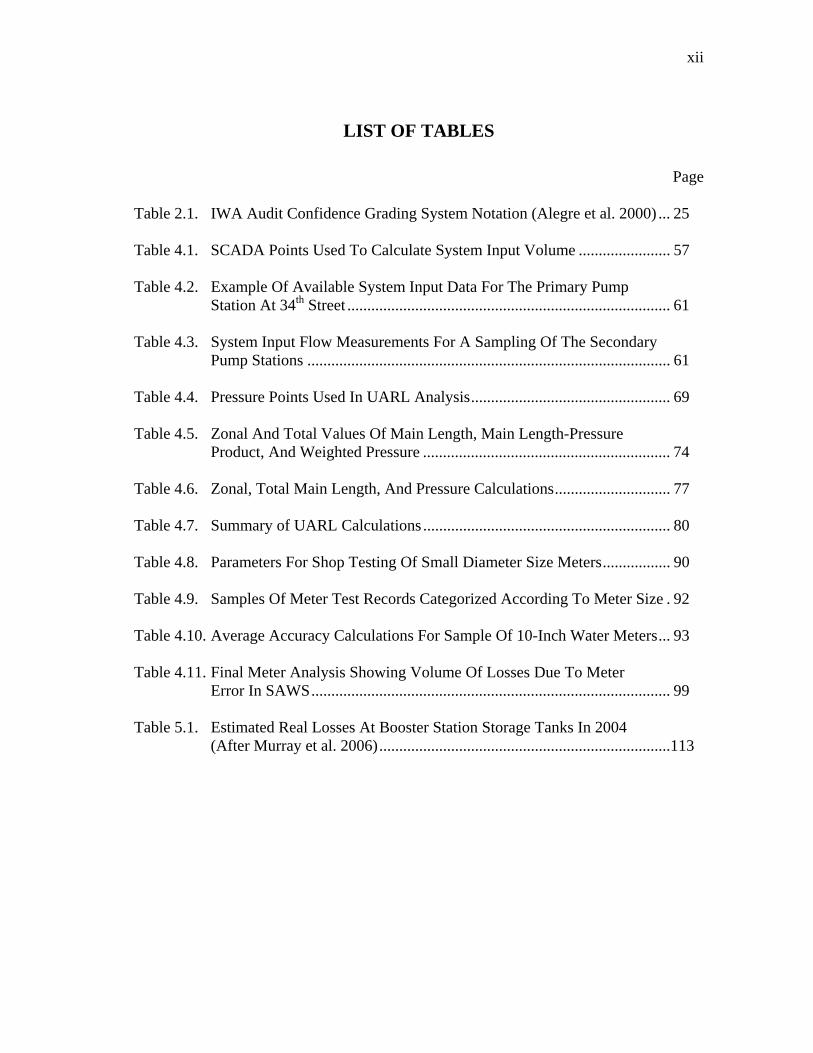
Fig. 2.1. International Standard Water Balance (Lambert et al. 2000)........................ 17 Fig. 3.1. Exhibit showing geographic location of San Antonio and area aquifers ...... 40 Fig. 3.2. Exhibit showing Edwards Aquifer contributing, recharge, and transition zones.............................................................................................. 41 Fig. 3.3. Water demand projections (after SAWS 2005)............................................. 46 Fig. 3.4. Schematic diagram of a typical SAWS primary pumping station................. 47 Fig. 3.5. Schematic diagram of a typical SAWS secondary pumping station............. 48 Fig. 3.6. Past and projected per capita consumption for SAWS (SAWS 2005).......... 51 Fig. 4.1. Map of pressure zones, pressure points, and water mains used in UARL analysis .......................................................................................................... 71 Fig. 4.2. Spatial analysis and calculation of the product of main length and system pressure for pressure zone 3 .......................................................................... 73 Fig. 4.3. Single year distribution system water balance (Brumbelow et al. 2006)...... 84 Fig. 4.4. Single year stored water balance with carryover quantities (Brumbelow et al. 2006)................................................................................ 86 Fig. 4.5. Distribution of water meters according to brand manufacturer .................... 91 Fig. 5.1. Water balance, adapted to SAWS, with finalized system input and output.. volumes .........................................................................................................102

xii

LIST OF TABLES

Page

Table 2.1. IWA Audit Confidence Grading System Notation (Alegre et al. 2000) ... 25 Table 4.1. SCADA Points Used To Calculate System Input Volume ....................... 57 Table 4.2. Example Of Available System Input Data For The Primary Pump Station At 34th Street ................................................................................. 61 Table 4.3. System Input Flow Measurements For A Sampling Of The Secondary Pump Stations ........................................................................................... 61 Table 4.4. Pressure Points Used In UARL Analysis.................................................. 69 Table 4.5. Zonal And Total Values Of Main Length, Main Length-Pressure Product, And Weighted Pressure .............................................................. 74 Table 4.6. Zonal, Total Main Length, And Pressure Calculations............................. 77 Table 4.7. Summary of UARL Calculations .............................................................. 80 Table 4.8. Parameters For Shop Testing Of Small Diameter Size Meters................. 90 Table 4.9. Samples Of Meter Test Records Categorized According To Meter Size . 92 Table 4.10. Average Accuracy Calculations For Sample Of 10-Inch Water Meters... 93 Table 4.11. Final Meter Analysis Showing Volume Of Losses Due To Meter Error In SAWS.......................................................................................... 99 Table 5.1. Estimated Real Losses At Booster Station Storage Tanks In 2004 (After Murray et al. 2006).........................................................................113

1

1. INTRODUCTION

The focus of this thesis is testing, evaluating, and improving a particular method

of water auditing. A water loss audit according to the standards and methodologies of

the International Water Association (IWA) was applied to a major North American

utility, the San Antonio Water System (SAWS), located in San Antonio, Texas.

Methodologies and procedures for conducting this type of water audit on a unique utility

were defined in areas where the guidelines are vague. The effectiveness of the audit

model was evaluated in the context of SAWS. Also, policy and resource allocation

recommendations were made for SAWS.

Water accountability describes a variety of activities affecting the water delivery

efficiency of water utilities. Standards for water accountability are increasing for many

water utilities as supplies are progressively strained (WSTB 2002). Growing

populations coupled with periods of drought have increased the demand on current water

supplies. Controlling losses in a water utility system is an efficient method of helping to

ensure there will be enough water supply to meet future demand. Most of the regional

water plans in Texas include conservation and loss reduction as a significant component

of “new supply” for the next 50 years (TWDB 2002). One particular water

accountability and conservation technique, which is presently gaining popularity, is

water auditing. Completing a water audit on a utility system is essentially comparing the

_______________________ This thesis follows the style of the Journal of Water Resources Planning and Management.

2

volume of water input with the volume of water output. A water audit can tell how

much water is lost from the system as well as pinpoint sources of revenue loss. Water

losses can arise from various reasons including theft, poor accounting, operational error,

and leaking pipes to name a few. Currently, the United States does not have any

national agenda to minimize water lost by suppliers (Thornton and Kunkel 2002).

Instead, the focus of water accountability has been primarily on the demand-side, for

example, consumer based conservation. However, focusing on the supply-side of water

accountability has many advantages including the reduction of adverse environmental

impacts. According to Thornton and Kunkel (2002), “high losses directly require

oversized infrastructure, excess energy usage, and unneeded withdrawals or abstractions

from source water supplies, all of which have potentially unnecessary – and sometimes

damaging – effects on the environment.”

1.1. THESIS STATEMENT

Although it is a beneficial tool for water resources management, the IWA water

auditing process needs refinement to be applicable to many North American water

utilities. To test this hypothesis, the IWA water auditing methodologies, as outlined in

the manual entitled Performance Indicators for Water Supply Services (Alegre et al.

2002) were applied to SAWS for the year 2004, and new techniques were proposed and

evaluated. The following questions were addressed after completion of the water audit.

1. What are the apparent improvements of the IWA water auditing techniques when

qualitatively compared to the most commonly used auditing method in North

3

America (the American Water Works Association M36 Manual entitled Water

Audits and Leak Detection [AWWA 1999])?

2. What are the limitations of the IWA water auditing process when applied to

North American utilities and how can it be improved? The IWA water audit is a

standard and detailed set of procedures set forth to accurately capture all aspects

and inefficiencies in a water system. Inevitably, the model outlined came up

short in some instances of the application to SAWS. The model lacked

flexibility to completely and accurately portray the uniqueness of the specific

water system being analyzed. Improvements upon the IWA methodologies have

been formulated to better capture all characteristics and processes taking place

within SAWS. These suggested improvements may enable SAWS and other

utilities to perform better audits in future years.

3. What are the most critical inefficiencies for the particular case of SAWS?

Furthermore, what policies may help to reduce these inefficiencies? The IWA

water audit uses a water (mass) balance model to quantify all volumes of water in

the system over the one year study period. This model is the essence of the IWA

water audit, and upon audit completion the water balance volumes can be

compared side by side to understand where the system losses are occurring,

where utility management resources should be focused, and where improvements

should be made. This research identified the most critical inefficiencies in the

SAWS, as well as made suggestions for operational procedures to address the

issues identified.

4

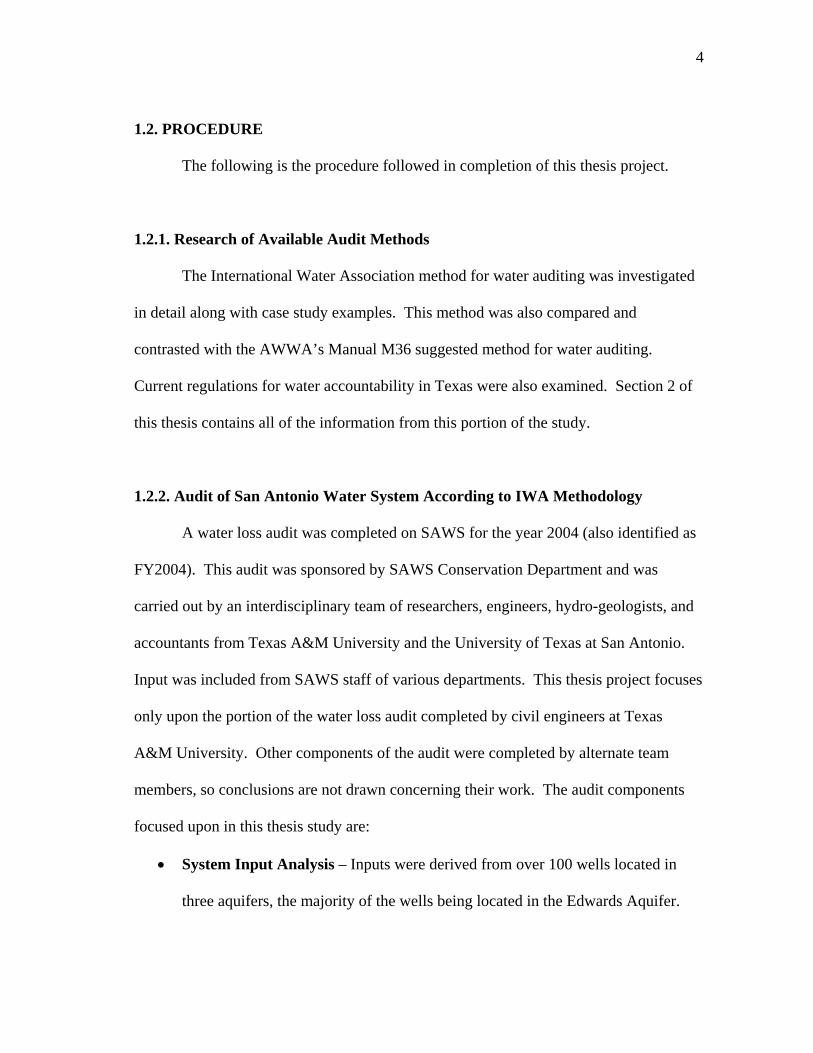
1.2. PROCEDURE

The following is the procedure followed in completion of this thesis project.

1.2.1. Research of Available Audit Methods

The International Water Association method for water auditing was investigated

in detail along with case study examples. This method was also compared and

contrasted with the AWWA’s Manual M36 suggested method for water auditing.

Current regulations for water accountability in Texas were also examined. Section 2 of

this thesis contains all of the information from this portion of the study.

1.2.2. Audit of San Antonio Water System According to IWA Methodology

A water loss audit was completed on SAWS for the year 2004 (also identified as

FY2004). This audit was sponsored by SAWS Conservation Department and was

carried out by an interdisciplinary team of researchers, engineers, hydro-geologists, and

accountants from Texas A&M University and the University of Texas at San Antonio.

Input was included from SAWS staff of various departments. This thesis project focuses

only upon the portion of the water loss audit completed by civil engineers at Texas

A&M University. Other components of the audit were completed by alternate team

members, so conclusions are not drawn concerning their work. The audit components

focused upon in this thesis study are:

• System Input Analysis – Inputs were derived from over 100 wells located in

three aquifers, the majority of the wells being located in the Edwards Aquifer.

5

• Unavoidable Annual Real Losses (UARL) Analysis – This calculation

estimated a volume of leaks from the system that are undetectable or would be

uneconomical to repair. UARL represents a level of allowable physical losses

from the system.

• Deferred Accounting System – A new method was formulated that incorporates

operation of an aquifer storage and recovery project into the standard water

balance notation.

• Customer Metering Inaccuracies – The standard water balance includes a

category determining the amount of water lost or gained due to incorrect meter

measurements. However, there are no guidelines for how this analysis should be

carried out. A procedure was created to determine metering inaccuracies in the

system.

1.2.3. Audit Limitations Identified and Resolved

This portion of the procedure was completed concurrently with performing the

water loss audit (section 1.2.2). During the application of the IWA audit to the SAWS,

several limitations of the audit were discovered. As each limitation was identified, a

solution was formulated. New methodologies were developed to incorporate the aquifer

storage and recovery project into the water balance accounting system and to calculate

UARL for a system with multiple pressure zones. Other difficulties encountered and

addressed were calculation of system input from multiple methods of volume

6

measurement and defining a procedure to estimate the accuracy of the system flow

meters.

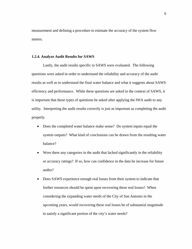
1.2.4. Analyze Audit Results for SAWS

Lastly, the audit results specific to SAWS were evaluated. The following

questions were asked in order to understand the reliability and accuracy of the audit

results as well as to understand the final water balance and what it suggests about SAWS

efficiency and performance. While these questions are asked in the context of SAWS, it

is important that these types of questions be asked after applying the IWA audit to any

utility. Interpreting the audit results correctly is just as important as completing the audit

properly.

• Does the completed water balance make sense? Do system inputs equal the

system outputs? What kind of conclusions can be drawn from the resulting water

balance?

• Were there any categories in the audit that lacked significantly in the reliability

or accuracy ratings? If so, how can confidence in the data be increase for future

audits?

• Does SAWS experience enough real losses from their system to indicate that

further resources should be spent upon recovering these real losses? When

considering the expanding water needs of the City of San Antonio in the

upcoming years, would recovering these real losses be of substantial magnitude

to satisfy a significant portion of the city’s water needs?

7

• What decisions and innovations were carried out by the research team during the

auditing process that would be beneficial for utilities to understand when

carrying out the audit themselves in future years?

• What are the benefits to the utility for completing this audit?

1.3. THESIS STRUCTURE

This thesis consists of five additional sections. Section 2 presents a literature

review, which compares and contrasts the International Water Association auditing

method with North America’s most common audit method, AWWA’s Manual M36. In

addition, section 2 discusses water loss audit requirements and trends in the State of

Texas. Section 3 presents useful background information which acquaints the reader

with unique characteristics of the City of San Antonio, such as climate, geography, and

population as well as water demand trends. Also presented is pertinent information on

the infrastructure components of SAWS, such as pumping and booster station

configuration, system pressure zone layout, available water sources for the utility, and

creation of the aquifer storage and recovery project. Section 4 clearly defines the

methodologies developed during this thesis research for various aspects of the water

audit including:

• Estimating the volume of water input into the distribution system.

• Calculating an economically allowable and unavoidable volume of leaks in the

distribution system. (UARL)

8

• Creating an accounting system for both yearly and continuous operations of the

aquifer storage and recovery project within SAWS.

• Determining losses due to under-registering water meters throughout the system.

Section 5 explains all results from the completed application of the IWA audit to SAWS.

A water balance is presented, which compares resulting volumes of water at various

points in the delivery cycle of the water system. This water balance diagram allows

various forms of non-revenue water in the system to be pin-pointed, so that plans can be

formulated to reduce these system losses in the future. Section 6 closes this thesis by

giving suggestions for conducting improved water audits in the future. This section also

advises the utility (SAWS) on what this audit concludes their current inefficiencies are,

and gives recommendations for addressing these issues.

9

2. REVIEW OF WATER AUDITING METHODS

Two of the most prevalent water auditing techniques currently used are discussed

in this section. In section 2.1, an overview of the currently endorsed method by the

American Water Works Association (AWWA) is discussed. This method is currently

under review and will soon be changed to reflect the methods used by the IWA. The

IWA water auditing method is discussed in great detail in section 2.2, since this method

is the focus of this research project. Sections 2.2.7.1 through 2.2.7.3 present case studies

of application of the IWA audit throughout the world. Next, section 2.3 discusses

present water accountability requirements by law in the State of Texas. This information

is also pertinent due to the fact that the IWA methods are being tested on a Texas utility.

Each of the three audit methods (AWWA, IWA, and State of Texas) will be analyzed

according to the following categories: Tasks/Method, Vocabulary, Input Data, Output

Results, Provisions for Error and Uncertainty, and Limitations. This will allow for easy

comparison between the three auditing methods.

2.1. AMERICAN WATER WORKS ASSOCIATION AUDIT METHOD:

MANUAL M36

The AWWA has announced that it will publish in 2007 a manual describing the

IWA water auditing process for use in the United States. It is the new AWWA Manual

M36 and is entitled Accountability and Loss Control Programs for Drinking Water

Utilities (Brumbelow et al. 2005). There are no federal regulations in the U.S. requiring

10

use of this forthcoming manual; however its creation – and endorsement by AWWA - is

a step closer to uniform water accountability practices in the United States.

The current AWWA Manual M36 was published in 1999 and is entitled Water

Audits and Leak Detection. Use of this manual is also not currently required in most

North American utilities; however it is the recommended method of water auditing

during the past decade. The following sections briefly outline the water auditing method

as explained by the 1999 Manual M36 as well as point out some of the shortcomings of

this water auditing method.

2.1.1. Tasks/Method

The AWWA Manual M36 audit is divided into the following tasks as described in

Chapter 2 of the manual (AWWA 1999).

1. Measure the Supply – Identify water sources. Measure water from each source.

Assess measurement accuracy from each source and adjust input volume

accordingly.

2. Measure Authorized Metered Use – Identify metered water uses. Measure

metered water uses. Assess meter accuracy and adjust amount of water used

accordingly.

3. Measure Authorized Unmetered Use – Identify and estimate amount of water

used by unmetered customers. These uses could include water used for

firefighting and training, flushing mains, storm sewers, and sanitary sewers,

11

street cleaning, schools or other public buildings, or water landscaping of public

parks.

4. Measure Water Losses – All volumes of water that do not fit the previous three

tasks by default are considered “unaccounted-for-water”. The object of task four

is to identify potential water losses and estimate the volumes of each type of loss.

These losses can include accounting errors, unauthorized connections,

evaporation of water stored, reservoir overflows, discovered leaks, reservoir

seepage and leakage, and any water lost due to malfunctioning equipment or

system controls.

5. Analyze Audit Results – Audit results define the calculation of two quantities.

The first is potential water system leakage which is total water loss minus all

measured water losses (from task 4). Total water loss is equivalent to system

input (corrected for meter errors) minus all authorized water uses. The second

result quantity this audit defines is recoverable leakage. This quantity is simply

the potential water system leakage multiplied by 50%, suggesting that half of all

potential leaks can be discovered and repaired.

2.1.2. Vocabulary

The following terms are useful to understand when conducting an audit

according to the AWWA Manual M36. Some of these terms are similarly defined in

section 2.1.1. Definitions are paraphrased from the Manual M36 (AWWA 1999).

12

• Supply is defined as water supplied to the system that has been adjusted for

metering inaccuracies and changes in storage (reservoir or tanks) for the audit

period.

• Authorized Metered Use is defined as water used by registered customers who

have metered connections. Adjustments are made for metering inaccuracies.

• Authorized Unmetered Use is defined as water used for allowable uses, but not

through a metered connection.

• Water Losses are defined as water that is consumed that does not generate

revenue for the utility, or water that is physically lost from the system (leaks).

There are two additional phrases associated with the Manual M36 audit.

• Accounted-for-water is defined as “water that is either metered or used for an

authorized, unmetered use” (AWWA 1999).

• Unaccounted-for-water is defined as “water that is neither metered nor

authorized. This water is considered lost from the system. The water does not

produce revenue and is not available for beneficial uses.” (AWWA 1999) The

previously discussed concept potential system leakage is included in

unaccounted-for-water.

13

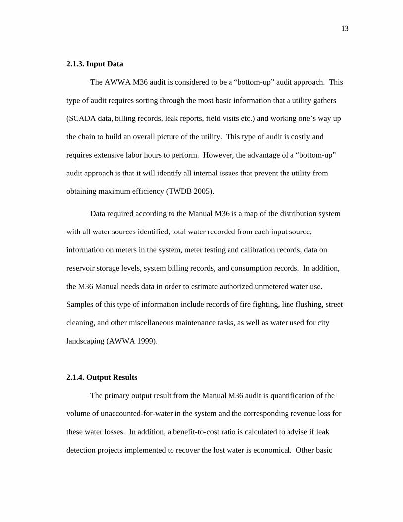
2.1.3. Input Data

The AWWA M36 audit is considered to be a “bottom-up” audit approach. This

type of audit requires sorting through the most basic information that a utility gathers

(SCADA data, billing records, leak reports, field visits etc.) and working one’s way up

the chain to build an overall picture of the utility. This type of audit is costly and

requires extensive labor hours to perform. However, the advantage of a “bottom-up”

audit approach is that it will identify all internal issues that prevent the utility from

obtaining maximum efficiency (TWDB 2005).

Data required according to the Manual M36 is a map of the distribution system

with all water sources identified, total water recorded from each input source,

information on meters in the system, meter testing and calibration records, data on

reservoir storage levels, system billing records, and consumption records. In addition,

the M36 Manual needs data in order to estimate authorized unmetered water use.

Samples of this type of information include records of fire fighting, line flushing, street

cleaning, and other miscellaneous maintenance tasks, as well as water used for city

landscaping (AWWA 1999).

2.1.4. Output Results

The primary output result from the Manual M36 audit is quantification of the

volume of unaccounted-for-water in the system and the corresponding revenue loss for

these water losses. In addition, a benefit-to-cost ratio is calculated to advise if leak

detection projects implemented to recover the lost water is economical. Other basic

14

results of the Manual M36 audit are the final volume of water supplied to the system

after adjustments have been made, final volume of authorized metered water use, final

estimated volume of authorized unmetered water use, and final estimates of measured

water losses in the system.

2.1.5. Provisions for Error and Uncertainty

AWWA’s Manual M36 has no provisions for determining error and uncertainty in data

or audit results.

2.1.6. Limitations

The following are weaknesses that have been cited regarding AWWA’s Manual

M36 water auditing methods. (These shortcomings have been corrected by the IWA

auditing method.) First, the current M36 method lacks performance indicators which

give an overall assessment of all aspects of the utility system performance and allow a

standard of comparison between utility systems. The Manual M36 uses the term

“unaccounted-for-water” to represent any volume of water that cannot be measured or

attributed a revenue value. This definition is much less specific than the IWA method

for defining non-revenue water, where every drop is counted and its point of loss in the

system is identified. Lastly, the IWA method is used much more widely than AWWA’s

auditing method. IWA is used in 20 different countries for at least 27 water systems

(Kunkel 2002a), whereas the AWWA auditing method is used only in North America on

15

a limited and voluntary basis. In general, North America is in need of a consistent and

well defined water loss accounting procedure.

There are a couple of problematic issues associated with many other North

American water loss auditing formats. Although these problems are not specifically

found in the Manual M36, the following methods are commonly used and information is

misrepresented. First, since there is no standard definition for a minimum allowable

level of leakage from the system (IWA calls this unavoidable annual real losses –

UARL) each utility defines this acceptable level for themselves. In many instances they

include discovered leaks and storage overflows as part of authorized consumption

instead of including these in the loss category (Kunkel 2002a). Another inconsistency in

North American audits is reporting the system’s water loss estimate as a percentage of

their system input instead of as a yearly volume. Per capita water usage is high in North

America, especially in comparison with the rest of the world. Reporting loss as a

percentage of input undervalues the magnitude of the water losses because the

corresponding water system inputs are also large (Kunkel 2002a). Reporting water

losses in units of volume makes the issue of waste more specific than reporting losses as

a system wide percentage. Making this information publicly available will inform

customers of water accountability issues, so that they too can be involved in

conservation on the demand side as well as encouraging their utility to conserve (and

remedy losses) on the supply side.

16

2.2. INTERNATIONAL WATER ASSOCIATION AUDIT METHOD

It is important to clearly explain this water auditing technique because it is

becoming the standard for audits in the United States. It is already deemed the gold

standard in water accountability practices and is used in numerous locations

internationally, such as Great Britain, South Africa, Italy, Australia, and New Zealand

(Kunkel 2002a). In the year 2000, the International Water Association (IWA) published

their auditing manual entitled, Performance Indicators for Water Supply Services. This

method was developed in Great Britain and was motivated by a drought they suffered in

the mid 1990’s. It has proved to be an effective water accountability method for their

country. The following sections will explain the IWA auditing method according to the

six specified categories.

2.2.1. Tasks/Method

The essence of the IWA Audit Methodology is the International Standard Water

Balance shown in the following Fig. 2.1 (Lambert et al. 2000).

17

Fig. 2.1. International Standard Water Balance (Lambert et al. 2000).

In the IWA water balance diagram, each column is a different notation for describing the

same volume of water at some point in the delivery cycle of the utility system.

Likewise, each aligned row totals the same volume of water. Performing an IWA audit

involves quantifying each entry (volume per year) in Fig. 2.1. Depending upon the size

of the utility system, quantifying each of these entries can become an arduous process of

sifting through SCADA (supervisory control and data acquisition system) information,

billing records, and leakage reports, meter testing records, and so on. By quantifying all

entries in the water balance, the utility company can build a complete picture of their

system efficiency and determine where to focus their resources to produce the greatest

amount of improvement.

The IWA audit is considered to be a “bottom-up” audit approach. This type of

audit requires sorting through the most basic information that a utility gathers (SCADA

data, billing records, leak reports, field visits etc.) and working one’s way up the chain to

build an overall picture of the utility. This type of audit is costly and requires extensive

18

labor hours to perform. However, the advantage of a “bottom-up” audit approach is that

it will identify all internal issues that prevent the utility from obtaining maximum

efficiency (TWDB 2005).

2.2.2. Vocabulary

It is important to comprehend some of the common terminology used in the

water balance diagram (Fig. 2.1), which is also used in the IWA audit manual. This

vocabulary is important because its use is becoming common place among those who

study water accountability and formulate water policy for countries, states, and planning

regions throughout the world. As will be made clear in section 2.3 of this paper

(focusing on Texas), the common use of the audit terminology is the first sign that the

IWA auditing method is spreading in the water accountability world. This terminology

is also important because it is replacing a sub-par method of water accountability that

used the general term “unaccounted-for-water” to describe all water in the utility system

that for any number of reasons did not earn revenue for its use by consumers. All of the

following definitions paraphrased from a book entitled Water Loss Control Manual

(Kunkel 2002a) are specific forms of “unaccounted-for” or non-revenue water.

• Real Losses are physical losses from the distribution system. Examples are pipe

main leaks, service connection leaks, bursts, system blow-offs, and storage tank

overflows. These losses are charged at the wholesale cost of water because they

occur before the water reaches the customer.

19

• Apparent Losses is water that reaches a customer or other end user, but is not

properly measured or tabulated. Examples are inaccurate customer billing

records, inaccurate customer metering (a larger amount of water reaches the user

then the meter registers), and unauthorized consumption (theft) of water. These

types of losses are charged at the customer retail cost of water.

• Unbilled Authorized Consumption is metered or unmetered water used by

registered customers, the water supplier itself, or others who are implicitly or

explicitly authorized to do so by the water supplier. Examples are water used for

fire-fighting, public buildings such as schools, the courthouse, police department,

etc. which may be granted free use of water.

It is also important to understand the definitions of the water balance components

shown in the last column of the water balance, Fig. 2.1. This last column symbolizes the

various ways that the utility system output can be described and quantified.

• Billed Exported Water is water sold to other utility companies.

• Billed Metered Consumption is the amount of water used by metered paying

customers.

• Billed Unmetered Consumption is use of water by customers who do not have

meters, but do pay for use of water. These customers’ water use is likely

estimated by a utility approved procedure, or they are simply charged at a flat

rate per month.

20

• Unbilled Metered Consumption is water used by public facilities (city parks,

court houses, schools, etc). Authorized users meter the water they consume, but

they don’t have to pay for it.

• Unbilled Unmetered Consumption is for authorized city uses like fire-fighting,

street cleaning, line flushing etc, which are typically unmetered.

• Unauthorized Consumption is an apparent loss where water is lost due to theft

through illicit connections or tampering of meters so they will under-register.

• Customer Metering Inaccuracies is an apparent loss where water is lost due to

under-registering meters. Meters more commonly under-register than over-

register; however a meter accuracy analysis will determine the behavior present

in the particular system.

• Leakage on Mains is a real loss where water physically leaks from the pipes.

• Leakage and Overflows at Storages is a real loss where water physically

overflows from storage tank reservoirs.

• Leakage on Service Connections up to Point of Customer Metering is a real

loss between the service connection and the water main.

• Unavoidable Annual Real Losses (UARL) – UARL is not shown specifically

on Fig. 2.1, however it is a subsidiary category of the three types of leakage

listed. UARL is an allowable volume of leaks, which occur at these three

locations (mains, service connections, and storage tanks).

21

2.2.3. Input Data

Section 4.1 of this thesis expands upon the type of data used in the audit

analysis. The IWA audit is also considered to be a “bottom-up” audit approach.

Therefore, the data used is similar to that used in the M36 Manual audit. The most

important input data is SCADA data for metered flows, measured pressures, and pump

run times. Also used was billing records, consumption records, leak detection reports,

field visits, meter accuracy testing records, and day to day operational information from

utility employees.

2.2.4. Output Results

The major product of an IWA audit is the water balance with values assigned to all

system output quantities for easy comparison of non-revenue water categories. Another

significant result of an IWA audit is a list of performance indicators. Section 2.2.5.1

describes performance indicators in detail. In addition, each piece of data used in

calculation of the performance indicators and in determining final volumes for the water

balance is assigned both an accuracy and reliability value. This is termed confidence

grading of data and is expanded upon in section 2.2.5.1 of this thesis.

2.2.4.1. Performance Indicators

The IWA auditing manual outlines the necessary audit calculations in a very

detailed step-by-step process. It divides all aspects of a water utility system into six

categories of performance indicators (PI). The IWA audit manual (Alegre et al. 2002)

22

defines performance indicators as “a quantitative measurement of a particular aspect of

the utilities’ performance or standard of service. They assist in the monitoring and

evaluation of the efficiency and effectiveness of the utility.” These indicators are as

follows:

• Water Resources Indicators

• Personnel Indicators

• Physical Indicators

• Operational Indicators

• Quality of Service Indicators

• Financial Indicators

Within each of the six performance indicators listed above are sub-categories that

further quantify smaller pieces of the water system performance. These sub-categories

are the pieces of the audit that contain specific formulas for data to be input and

calculated. For example, the Operational Indicator section of the audit contains sub-

categories that allow the auditor to quantify leakage control, pump refurbishment,

calibration of water level meters, apparent losses and real losses just to name a few of

the needed calculations.

PIs are of beneficial use to all stakeholders of a utility. For the utility

themselves, the PIs identify the strengths and weaknesses of different divisions of the

utility and provide a benchmark each auditing period to measure self-improvement or

comparison with other utilities. Regulatory agencies are another important stakeholder

group in the system. For regulatory agencies, PIs allow the utilities to be easily

23

monitored and ensure compliance with any laws or policies of the governing body. The

governing policy-makers are important stakeholders and have interest in the audit and

PIs so that they can compare utilities’ performances, identify problems, and formulate

policies to guide and correct issues of public concern (Alegre et al. 2002).

One of the most useful PIs in the IWA audit is named the infrastructure leakage

index (ILI). It is new to the IWA auditing methodology and not normally quantified in

other North American audits. The ILI is a unitless ratio comparing the volume of annual

real losses (all physical losses from the system) to the volume of unavoidable annual real

losses (physical losses that are undetectable or uneconomical to repair).

Annual Real LossesILI=UARL

(2.1)

Since the ILI is a ratio and not a percentage of annual consumption, the ILI value can be

compared between any utility (using these IWA calculation methods) anywhere in the

world. According to Kunkel (2002) “The ILI ratio is a great way to demonstrate loss

management performance, as each system effectively compares the ratio of its individual

best possible performance against how it is actually performing.” An ILI of 1.0 is ideal

but not economically feasible to achieve until water becomes a much more expensive

commodity or becomes a scarce resource. ILI values between 1.5 and 2.5 are considered

satisfactory for most utility systems (Kunkel 2002a). For comparison purposes, a

sample of seven North American utilities, an average ILI of 7.37 was determined

(Lambert et al. 2000).

24

2.2.5. Provisions for Error and Uncertainty

The IWA auditing method evaluates the error and uncertainty of all data used in

the audit, and then assigns reliability and accuracy values for all final results. IWA has

termed this uncertainty analysis confidence grading of data and it is described in detail

in section 2.2.5.1.

2.2.5.1. Confidence Grading of Data

Confidence grading of data is an important attribute of performing an IWA water

audit because it quantifies the reliability and accuracy of each piece of information. The

confidence grading scheme that is outlined in the IWA auditing manual was developed

so that when using the performance indicators, the reliability of the data is known and

taken into consideration when performing calculations. Possible errors in the data

collected must be evaluated and assessed. Each performance indicator calculation is

given a confidence rating which describes both how accurate and reliable the

information is believed to be. These confidence ratings can also be used to dictate how

to improve the system efficiency in the future. If the audit finds that there is little

confidence in the accuracy of the meters on the well pumps, then possibly these meters

should be replaced or calibrated more often on a routine schedule.

Table 2.1 summarizes the reliability and accuracy ratings that each performance

indicator calculation can be given according to the IWA auditing manual.

25

TABLE 2.1. IWA Audit Confidence Grading System Notation (Alegre et al. 2000)

Reliability Rating Accuracy Rating

A = highly reliable 1 = (+/-) 1%

B = reliable 2 = (+/-) 5%

C = unreliable 3 = (+/-) 10%

D = highly unreliable 4 = (+/-) 25%

5 = (+/-) 50%

6 = (+/-) 100%

X = Values Outside the Valid Range

As an example, according to Table 2.1, a data value given the confidence grading of

“B3” is described as a reliable data value with a likely accuracy of plus or minus ten

percent of the given value.

2.2.6. Limitations

The IWA audit, like any model, has its limitations. When applying the IWA

methods to SAWS, a few weaknesses were discovered. First, the IWA audit method was

not defined to accommodate the operation of SAWS aquifer storage and recovery

system. This weakness arises when the utility has a facility which accommodates over-

year storage and the distribution system acts as a transmission system to move water

between production and storage facilities. To remedy this problem, a deferred

accounting system was developed to work in conjunction with the traditional IWA water

balance after slight modifications were made. The second limitation recognized was the

26

absence of guiding procedures to calculate the system’s UARL. SAWS, similar to many

utilities, has a varied topography and consequently multiple pressure zones, booster

stations, and pressure reducing valves throughout the distribution system. This

complexity leads to difficulty in calculating an average system pressure, which is one of

the inputs into the empirically derived UARL equation. A spatial analytical method was

developed to address this variability in system pressure and to provide guiding

procedures for calculation UARL in future audits (Brumbelow et al. 2006).

2.2.7. IWA Audit Case Studies

Three case studies are presented where the IWA audit has been applied very

successfully. Lessons can be learned from these case studies, as well as from the most

current case study; application of IWA audit methodologies to SAWS.

2.2.7.1. Great Britain (Thornton and Kunkel 2002a)

Great Britain privatized their water utility companies in 1989. Later, in 1992, the

government began requiring that all water companies produce annual reports, which

followed a standard format quantifying water losses. Published nationally for all to read,

these reports made clear that the utilities were losing large amounts of water. Great

Britain experienced a severe drought in 1995 and 1996. This drought spurred further

government regulation (a National Leakage Initiative was began) and mandatory

minimum leakage targets were set. After five years of employing various leak detection

techniques, water auditing, and other water accountability methods, leakage from the

27

water supply systems was reduced by 40 percent, or approximately 480 million gallons

of water per day. This is a fantastic accomplishment, and Great Britain is known

internationally for their leak detection methods, auditing methods (the IWA water audit),

and their success with privatization. These accomplishments in reducing water losses by

such a great percentage may not have been possible if the following had not been

required of them:

• Completing annual water loss calculations for every water utility system in the

nation.

• Requiring a standard format (IWA method) for carrying out calculations, using

performance indicators, and confidence grading of data.

• Publishing water loss results, creating public accountability for the efforts.

2.2.7.2. Philadelphia, Pennsylvania, USA (Kunkel 2002b)

Philadelphia is one of the oldest cities in the United States, and therefore has one

of the oldest water systems (over 200 years old), which has historically also been one of

the most progressive water systems. The Philadelphia Water Department (PWD)

reached its climax of water service in the mid 1950’s, supplying on average 377 MGD of

water to customers. By 2001, this rate had decreased to 270 MGD due to loss of

industry and urban sprawl. In the 1970’s and 1980’s, the PWD conducted a variety of

studies to determine their amounts of unaccounted-for-water. They soon realized their

water losses were quite high; therefore they began employing accountability measures

such as master meter calibration, meter replacement, and leak detection technology.

28

Even after these efforts, unaccounted-for-water levels remained near 100 MGD. A hike

in water tariff rates in 1993 created much public attention to water accountability issues

and soon a Water Accountability Committee was formed to pursue solutions to the PWD

losses.

The Philadelphia Water Accountability Committee worked closely with the

AWWA’s Leak Detection and Water Accountability. This group formulated a water

auditing process, which the PWD executed for the first time in 1996. This format for

water auditing soon was published by the AWWA as their Manual M36. Philadelphia

continued this type of audit for the next couple of years. George Kunkel, of the PWD,

became chair of the AWWA Leak Detection and Water Accountability Committee in

1998. During this time period, other internationally recognized experts joined the

committee, including Alan Lambert who chaired the IWA Task Force on Water Loss

and is a known leader and promoter in leakage management techniques. Kunkel

directed the group in exploring international water auditing methods and tested the

applicability of these methods to North American water utilities. Under Kunkel’s

research and direction, the PWD transitioned to use of the IWA audit methodology in

2000. The PWD hired international experts to assess the utilities losses. In addition to

completing the IWA audit, a sub-contractor was hired to perform night flow analysis and

other field measurements to supplement the audit.

PWD audit results according to IWA methodology determined that the utility

experience 94.7 MGD of non-revenue water. This quantity was further broken down to

be equivalent to 18.6 MGD of apparent losses, 70.2 MGD of real losses, and 5.9 MGD

29

of authorized unbilled usage. These losses were equated to a financial loss of $16.7

million.

The application of the IWA water audit to Philadelphia is important because it is

the first time this audit was used in North America. The IWA audit methodology was

tested and refined during this application. George Kunkel of the PWD continues to be a

leader in the field of water accountability and an ambassador for integrating and sharing

this international method of water loss control with North America’s recognized

authority on water, the AWWA. The PWD makes their IWA audit available for all to

see. It is in the format of a series of Microsoft Excel spreadsheets and was reviewed

extensively by the research team before completion of the SAWS IWA audit.

2.2.7.3. São Paulo, Brazil (de Freitas and Paracampos 2002)

The São Paulo Water and Sewer Company (SABESP) provides water and sewer

services to the metropolitan region of São Paulo, inhabited by 17 million people. Since

1995, SABESP has been undergoing a large reorganization and has put forth significant

efforts to increase their system efficiency and reach both their financial and operational

goals. To help reach these goals, SABESP has conducted water audits according to the

IWA methodology, which have produced great benefits to their utility. Their first IWA

water audit (in 1997) indicated that 13 percent of the apparent losses the utility was

experiencing were due to fraud (illicit connections). In response to this startling statistic,

they put resources into training staff to reduce fraud. This involved increasing the

number of inspections to 4,500 monthly. Of the inspections conducted, roughly five

30

percent lead to the discovery of fraudulent actions which has led to the recovery of about

800 cubic meters of water per case. In addition to increased inspections, SABESP began

paying contractors based upon the quality of their work in order to motivate excellence

in the field for system repairs. This case study is a wonderful illustration of how an

IWA audit can pinpoint the areas within a utility which need attention, more resources,

and investigation in order to increase overall system efficiency.

2.3. TEXAS WATER DEVELOPMENT BOARD REQUIREMENTS

In 2003, the 78th Texas Legislature created House Bill 3338, which amended

Section 16.0121 of the Texas Water Code to require every public utility which supplies

potable water to conduct a water loss audit once every five years. A standard auditing

format was created by the Texas Water Development Board (TWDB) and is available on

their website (http://www.twdb.state.tx.us). The audit results were reported to the

TWDB who in turn compiled the information submitted. The Legislature and Regional

Water Planning Groups will review the information in order to identify appropriate and

efficient water management strategies for the future. The first required water loss audit

used data collected from the 2005 calendar or fiscal year. Utilities filled out a simple

standard three page form, which were due by March 31, 2006.

31

2.3.1. Tasks/Method

2.3.1.1. Current Requirements in the State of Texas

The TWDB publishes a manual entitled Water Loss Manual, which describes

Texas’s auditing requirements, terminology, water balance, how to carry out the

calculations on the audit worksheet and much more. After examining this manual and

the Texas water audit reporting form, it is clear that both are based upon the ideas and

methodologies of the IWA audit. The introduction to the TWDB Water Loss Manual

states:

“The new methodologies being used enable water utilities to operate very efficiently. Based on the International Water Association’s methodology which has been used all over the world and recently in the United States, these methods are proven to work. They eliminate unaccounted for water, and the end results direct focus to problem areas.”

The Texas audit is only three pages in length and lacks the detail and data confidence

grading system of the IWA audit, but the water balance that it is based upon is identical,

the terminology is the same, and it introduces the idea of performance indicators only

when calculating real water losses. The Texas water audit addresses four main points of

water loss: loss from distribution lines, meter inaccuracies, deficiencies in accounting

methods, and water theft (TWDB 2005).

32

2.3.1.2. Looking to Future Requirements in Texas

After reading the TWDB’s Water Loss Manual, it is obvious that the State of

Texas agrees with the methodology of the IWA audit. Information was obtained from

Mr. Mark Mathis with the Municipal Water Section of the TWDB. Mr. Mathis, who is

responsible for assimilating the water audit policy, was asked what he thought the future

held for Texas water auditing policies and if he thought the State of Texas would

progress to requiring complete annual audits according the IWA methodology. Mr.

Mathis replied that ideally they would, but of course all is dependent upon the legislature

and what they decide to do in 2007. He agreed that a bottom-up approach would be best,

but that most of the utility systems in Texas serve less than 50,000 customers and would

thus not have the financial means or employee resources to conduct this type of in-depth

audit. Mr. Mathis said that the original HB 3338 was written to require audits annually,

but this constraint was changed to every five years in order to help the bill pass. In

conclusion, he stated that for now, the State of Texas is content with knowing how well

water is tracked by each utility. They are satisfied with introducing a consistent

methodology that has categories for each type of water use while also associating a cost

to that use.

2.3.2. Vocabulary

The vocabulary used in Texas Water Loss Control Manual is identical to the

IWA audit vocabulary with the following exception.

33

• Balancing Error is defined as the difference between system input and system

output in the water balance diagram. Theoretically, the two quantities should be

identical. The TWDB has created this term, balancing error, to make it appear

acceptable in instances when system input does not equal system output. When

systems have balancing errors, it indicates that the information input into the audit

should be reviewed and the validity of the estimates made in the audit should be

considered (TWDB 2006).

2.3.3. Input Data

This Texas water loss audit is considered a top-down audit, meaning it “utilizes

data the utility should already have without additional fieldwork. Data is transferred

from other reports to the water audit form, enabling the utility to see which areas warrant

more fieldwork” (TWDB 2005). Examples of input data required is system input

volume, meter accuracy, records for authorized water consumption, billing

adjustments/waivers records, unauthorized consumption estimates, storage tank overflow

estimates, water lost due to main breaks/leaks, water lost due to customer service

connection breaks/leaks, and financial records for the utility.

2.3.4. Output Results

The major result of this audit is quantifying both apparent and real losses.

Similar to the IWA audit, apparent losses include customer metering inaccuracies,

billing adjustments and waivers, and unauthorized consumption. Also similar to the

34

IWA audit, real losses include storage tank overflows, water main breaks and leaks, and

customer service line breaks and leaks. The Texas audit also has a few technical

performance indicators for real losses and financial performance to use in comparing one

utility to another. The indicators specified are (TWDB 2005):

• Total daily real losses divided by miles of main in system.

• Total daily real losses divided by number of service connections in system.

• Total cost of apparent losses.

• Total cost of real losses.

2.3.5. Provisions for Error and Uncertainty

The State of Texas Water Loss Control Manual has no provisions for

determining error and uncertainty in data or audit results. It only suggests that if a

balancing error is present in the system, then the validity of the data used should be

reviewed (TWDB 2006).

35

2.3.6. Limitations

This auditing method does not account for UARL, undocumented real losses, or

deferred accounting principles. Also, since this audit is a “top-down” audit, it does not

incorporate the detail or completeness that a “bottom-up” audit approach would capture.

This audit does not assess the reliability or accuracy of the data used in the calculations,

which is an important aspect of assessing the efficiency of the system and improving it

with each year. Another shortcoming of the TWDB audit method is the extremely

lenient requirements in its application rate of recurrence. Conducting the audit once

every five years is not frequent enough to capture patterns in water system behavior or

frequent enough to see if any policy changes enacted after the first audit are effective. It

is strongly recommended that the State of Texas require utilities to perform the audit

yearly. Last, the audit methodology according to the TWDB has provisions for a

balancing error in systems where system inputs do not equal system output. This is

essentially unaccounted-for-water and its addition to the audit neglects the whole point

of using IWA audit methodology in the first place.

36

3. OVERVIEW OF THE CITY OF SAN ANTONIO, TEXAS, AND

THE SAN ANTONIO WATER SYSTEM (SAWS)

The purpose of this section is to briefly describe the physical, geographical,

meteorological, and demographical characteristics of the region served by San Antonio

Water System as well as the extent of the infrastructure that is currently in use by the

utility. This background knowledge will put the unique qualities of this large utility into

context and allow for better understanding of general discussion on the system in

subsequent sections of this research report.

3.1. DEMOGRAPHICS, GEOGRAPHY, AND CLIMATE

According to the 2005 US Census population estimates, San Antonio, Texas is

the seventh largest city in the United States and is growing faster than most other large

American cities (Pearson Education 2006). The city’s population exceeded 1.2 million

in 2005, approximately a 9.8 percent increase since the year 2000 census. It is expected

that by the year 2050, the population in the SAWS service area will grow to nearly 1.8

million (SAWS 2005), an increase of about 50 percent. In the audit year, 2004, the per-

capita water consumption for the SAWS service area was 129 gallons per capita per day

(GPCPD). Through increased conservation efforts, SAWS expects the per capita water

consumption to decrease and stabilize around 116 GPCPD in a year with normal rainfall

amounts or 122 GPCPD during a dry year (SAWS 2005). Taking into consideration

these predictions for population increases and consumption patterns, SAWS expects its

37

water demand to increase by approximately 60,000 acre-feet per year or about 37

percent of current system input volumes by the year 2050 (SAWS 2005). SAWS is

always exploring opportunities for obtaining new sources of water supply to meet future

demands, whether it is by minimizing system losses, furthering conservation efforts, or

adding new water supply sources to its repertoire.

San Antonio is the county seat of Bexar County. There are two major water

supply utilities in Bexar County, serving residents of the City of San Antonio as well as

surrounding areas. These utilities are San Antonio Water System (SAWS) and Bexar

Metropolitan Water District (BexarMet). Each utility company has its own sources of

water. SAWS is the larger of the two systems, serving approximately 315,000 customer

connections at the end of the year 2004 (SAWS 2004). In 2006, BexarMet serves

approximately 80,000 customers connections (Bexar Met Water District 2006). SAWS

is owned by the City of San Antonio. On the other hand, BexarMet was created by the

Texas Legislature in 1945 as a stand alone agency to serve a residential housing boom in

San Antonio and has since then grown by taking over ownership of many small

independently owned utilities, spread disjointedly throughout the area (Bexar Met Water

District 2006).

The City of San Antonio is geographically located in south-central Texas,

approximately 140 miles from the Gulf of Mexico. According to the 2005 United States

Census, the city covers 412.07 square miles. The city sits along a geologic feature

named the Balcones Escarpment, which is an inactive normal fault line running from

38

southwest to north-central Texas forming the boundary between the hill country (to the

north) and the coastal plains (to the southeast) (Collins et al. 1997 and SAWS 2006d).

Fig. 3.1 shows the location of the city with in the State of Texas. This geographic

location is unique, contributing to the dynamics of the Edwards Aquifer and is the reason

behind the fresh water springs in the area such as the Comal Springs, the San Marcos

Springs, San Pedro Springs and many more in the region.

In San Antonio, monthly/average/annual precipitation amounts have been

recorded for the last 135 years, since 1871. Records show that the average annual

precipitation has been 29.05 inches (73.79 cm), with a maximum of 52.28 inches

(132.79 cm) and a minimum of 10.11 inches (25.68 cm) in one calendar year. The year

2004 (the year analyzed in this research project) has a record of 45.33 inches (115.14

cm) of precipitation occurring over the course of the year (National Weather Service

2005a). This amount of precipitation exceeds the annual average by 16.28 inches (41.35

cm) indicating that 2004 was a very wet year for the area. This information is important

when considering the scope of the water loss audit because excess rainfall over the

Edwards Aquifer Recharge Zone causes increased recharge and subsequently increased

water supply. In San Antonio, monthly/average/annual temperatures have been recorded

for the last 121 years, since 1885. Records show that the average annual temperature is

69.1 degrees Fahrenheit. July and August are the hottest months of the year and

consistently reach an average monthly temperature in the mid-eighties (National

Weather Service 2005b). During summer months, daily maximum temperatures are

normally in the nineties and sometimes reach 100 degrees Fahrenheit.

39

3.2. WATER SUPPLY SOURCES IN 2004

SAWS is effectively working towards diversifying its water sources, to counter

current over dependence upon the Edwards Aquifer. During the auditing year, 2004,

SAWS had three primary water sources which will be discussed in the following

sections. These sources and their corresponding percent of water supplied in 2004 are

the Edwards Aquifer (97.75%), the Trinity Aquifer (2.25%), and the Carrizo-Wilcox

Aquifer (0%). SAWS also considers its water reuse program to be a significant source

of water, however this program will not be discussed in this research project. Fig. 3.1

geographically shows the SAWS service area (outlined in black), the location of the

three pertinent aquifers, the location of SAWS well fields, and the location of SAWS

aquifer storage and recovery project.

3.2.1. Edwards Aquifer

The Edwards Aquifer is located along the Balcones Fault Zone in south-central

Texas. It is well known as one of the most productive and permeable aquifers in the

United States, serving more than 1.7 million people in the San Antonio area as well as

water for agricultural and industrial uses (Schindel et al. 2005). Geologically, the

Edwards Aquifer is comprised of Cretaceous-aged Edwards Group limestone, which has

formed a karst aquifer system. This means that the aquifer is a very well integrated

underground drainage system, like an underground river and has a high rate of

40

Fig. 3.1 Exhibit showing geographic location of San Antonio and area aquifers.

permeability (Schindel et al. 2005). The Edwards Aquifer has three major components;

the Contributing (drainage) Zone, the Recharge Zone, and the Artesian Zone, which are

shown in Fig. 3.2.

41

Fig. 3.2 Exhibit showing Edwards Aquifer contributing, recharge, and transition zones.

The Contributing Zone is located over the Edwards Plateau. In this area, rainfall

permeates the ground and forms a large water table where water forms spring fed

streams and runs downstream into the Recharge Zone. Fractures, faults, caves, and

sinkholes in the Edwards Limestone are exposed in the Recharge Zone. It is here that

the water quickly permeates into the aquifer, traveling through the karst system, and

flowing downstream to the Artesian Zone of the aquifer. The Artesian Zone

(“transition” in Fig. 3.2) is where most wells are located. This zone crosses through the

center of the City of San Antonio. In many places there is even enough pressure in this

42

zone that water erupts from the surface forming springs and artesian wells (Edwards

Aquifer Authority 2006a).

The Edwards Aquifer, until recently, was the sole water source for the City of

San Antonio. In 1993, the Texas Legislature passed an act forming the Edwards Aquifer

Authority (EAA) whose mission is to “manage, enhance, and protect the Edwards

Aquifer System” (Edwards Aquifer Authority 2006b). Due to this special legislative

action, the EAA has authority to regulate the amount of water SAWS, as well as any and

all other consumers can pump from the aquifer each year. In 2004, SAWS had the right

to pump up to 228,000 acre-feet of Edwards Aquifer water, where 38,000 acre-feet of

these rights were leased for short term usage (SAWS 2004).

3.2.2. Trinity Aquifer

The Trinity Aquifer is extensive and forms a belt through the center of Texas,

stretching from the Red River to the eastern boundary of Medina and Bandera counties.

It serves the metropolitan area of Dallas/Ft. Worth and is the primary water source for

much of the Texas hill country. Its permeability is much lower than the Edwards

Aquifer and it is not yet regulated by a single government entity. The Trinity Aquifer is

currently the topic of much political debate and its regulated status could very well

change in the next couple of years (Eckhardt 2006a).

On February 25, 2002 SAWS delivered the first water from wells located in the

Trinity Aquifer. This event pioneered the first non-Edwards Aquifer water to be

introduced to the SAWS water distribution system (SAWS 2006b). In 2004, there were

43

11 wells in the Trinity Aquifer, located at the Oliver Ranch and BSR property sites. In

February of 2000, SAWS signed a ten year contract to pump up to 4,500 acre-feet into

their distribution system, supplied from up to eight wells at Oliver Ranch (Needham

2000a). In September of 2000, SAWS signed a contract to purchase up to 1,500 acre-

feet of water per year from the BSR wells (Needham 2000b).

3.2.3. Carrizo-Wilcox Aquifer

The Carrizo-Wilcox Aquifer spans from the Rio Grande River in southwest

Texas to northeast Texas and into the state of Louisiana and Arkansas. This aquifer

crosses southern Bexar County and the SAWS service area as well as neighboring

counties Wilson and Atascosa. The Carrizo-Wilcox Aquifer is primarily sand with some

gravel, clay, silt, and lignite layers. Carrizo-Wilcox water can be treated by

conventional methods or used as is. Due to the relatively lower permeability of this sand

aquifer it is considered an ideal site for aquifer storage and recovery (ASR) (Eckhardt

2006b).

ASR is simply using an alternate aquifer to store surplus water for use at a later

date. It is an ideal method of storage for several reasons. First, water is stored

underground, so it is not subject to losses caused by evaporation like a surface reservoir.

Second, storing water at an ASR site allows the people who pay for the site’s

development to benefit from the water withdrawal in times of shortage. Third, a

primarily sand aquifer has a low permeability, meaning that when water is injected into

an unconfined sand aquifer it forms a stationary dome, or in a confined sand aquifer it

44

forms a horizontal layer around the well-pump. The water does not travel far, so it is

there; ready to be withdrawn at a later date (Eckhardt 2006b). This system is an ideal

solution to water shortages in the San Antonio area. The Edwards Aquifer is highly

permeable and in times of intense rainfall the aquifer level rises quickly, and causes the

connected streams to flood. In these times of surplus flow, water can be pumped from

the Edwards Aquifer, treated (this requirement by law), transported to an ASR site, and

injected into a sand aquifer for storage. In times of drought, this same water can be

pumped from the ASR site, back into the utilities distribution system.

In 1999 and 2000, SAWS purchased 3,200 acres of agricultural land in southern

Bexar County, over the Carrizo-Wilcox Aquifer (Needham 1999 and Needham 2000a).

Over the next few years, SAWS designed and constructed its first ASR facility named

the Twin Oaks Treatment Plant and Recovery Site. SAWS constructed several injection

wells, a water treatment plant, and connected this site to its water distribution system

with transmission lines. In February of 2002, to appease local interest groups, SAWS

stated that it would only pump water if a stage III drought occurred and it would not

pump more than 28,000 acre-feet over a period of two years from the ASR site

(Needham 2002). The ASR facility came online during the audit year 2004. SAWS

conducted routine tests, such as line flushing and injected approximately 1,809.5 MG of

water into the Carrizo-Wilcox Aquifer (Haby, J., personal communication, July 26,

2005).

45

3.3. PROJECTED WATER SUPPLY REQUIREMENTS

In 2005, SAWS published a study entitled Water Resource Plan Update. It is a

comprehensive review of a previous study completed in 1998 entitled Securing Our

Water Future Together, 1998 Water Resource Plan, which was approved by San

Antonio city council in 2000. This latest study has published projections for future

water supply needs through the year 2050. The task force who completed these

comprehensive studies formulated two scenarios: Planning Scenario 1 (PS1) and

Planning Scenario 2 (PS2). PS1 encompasses the current SAWS service area as well as

eight other small cities adjacent to SAWS service area. PS2 includes a much larger area,

and plans for SAWS to serve as a regional wholesale water provider for all areas

included in PS1 as well as the remainder of Bexar County (including BexarMet Water

Utility), and portions of Comal, Kendall, and Medina Counties (SAWS 2005). Only the

final results with regard to future water supply requirements will be discussed in this

research paper. If the reader would like further information, including methodology

behind these studies, please see these named SAWS studies which can be downloaded

from <http://www.saws.org/our_water/waterresources/waterresourceplan>.

Fig. 3.3 shows the predicted amounts of water required (in acre-feet) through the

year 2050 for PS1 and PS2 using a future per capita consumption of 122 GPCPD (cited

as the consumption for a dry, critical year planning period) and predicted population

growth estimates. In PS1, by the year 2050, an estimated 232,604 acre-feet of water will

be needed. In PS2, by the year 2050, an estimated 312,028 acre-feet of water will be

46

needed, keeping in mind that PS2 involves absorbing other existing utilities including

the sources of water for each additional utility.

Water Demand Projections

150,000

170,000

190,000

210,000

230,000

250,000

270,000

290,000

310,000

330,000

2005 2010 2015 2020 2025 2030 2035 2040 2045 2050

Year

Acr

e-Fe

et

PS1PS2

Fig. 3.3 Water demand projections (after SAWS 2005). 3.4. SAWS INFRASTRUCTURE

SAWS infrastructure and distribution system is extensive, making it one of the

largest water utilities in the United States. During the year 2004, SAWS increased their

customer base as well as their number of metered connections by 2.8% (SAWS 2004a).

It serviced a total of 315,116 potable water customers (SAWS 2004a) and maintained

4,324 miles of water main in their system (SAWS 2004). It can produce a maximum of

894.6 MGD and can store up to 159.6 MG of water (SAWS 2004a). SAWS has an

extensive Supervisory Control and Data Acquisition (SCADA) system in place. This

47

system constantly measures pipeline pressure at select points in the system, storage tank

levels, flow at the well meters, flow at the high service pumps, runtime at the high

service pumps, and many types of alerts, alarms, and water quality tests. The following

sections detail some of the most important infrastructure components in SAWS within

the context of a water loss audit.

3.4.1. Pumping Stations: Primary and Secondary

There are over 100 wells operated by the SAWS, currently located at 31 different

pumping stations. There are two types of pumping stations in the SAWS; primary and

secondary. Figs. 3.4 and 3.5 show each type of pumping station. In these two figures,

the clock pictured represents the “run-time constant” method of measurement and the

circle with the x inside represents the location of a flow meter. The squares with a “P”

inside represent high service pumps and the circles with a “W” inside represents a well

with a small well pump.

Fig. 3.4. Schematic diagram of a typical SAWS primary pumping station.

Storage Reservoir

P1

P2

P3

P4

P5

W1

W2

W3

W4

SL3 Distribution System

SL4 Distribution System

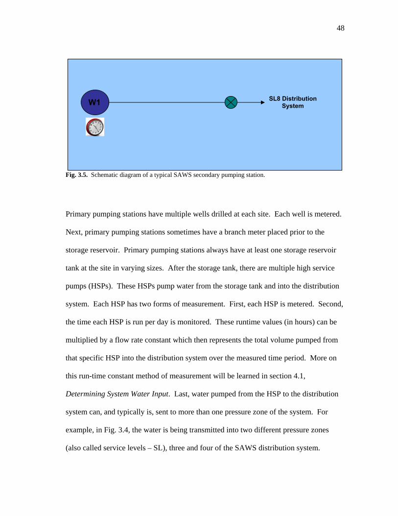
48

Fig. 3.5. Schematic diagram of a typical SAWS secondary pumping station.

Primary pumping stations have multiple wells drilled at each site. Each well is metered.

Next, primary pumping stations sometimes have a branch meter placed prior to the

storage reservoir. Primary pumping stations always have at least one storage reservoir

tank at the site in varying sizes. After the storage tank, there are multiple high service

pumps (HSPs). These HSPs pump water from the storage tank and into the distribution

system. Each HSP has two forms of measurement. First, each HSP is metered. Second,

the time each HSP is run per day is monitored. These runtime values (in hours) can be

multiplied by a flow rate constant which then represents the total volume pumped from

that specific HSP into the distribution system over the measured time period. More on

this run-time constant method of measurement will be learned in section 4.1,

Determining System Water Input. Last, water pumped from the HSP to the distribution

system can, and typically is, sent to more than one pressure zone of the system. For

example, in Fig. 3.4, the water is being transmitted into two different pressure zones

(also called service levels – SL), three and four of the SAWS distribution system.

W1 SL8 Distribution System

49

Secondary pumping stations are normally much simpler than the primary

pumping stations. They are comprised of a single well which is connected to a single

well pump. This well pump transmits water to a single pressure zone in the SAWS

distribution system. The well pumps at secondary pumping stations are metered and

each pump’s run-time is monitored. Usually, secondary pumping stations do not have

storage tank reservoirs, do not service more than one pressure zone, and although run

time is recorded in the SCADA system, run-time constants are not always derived for the

well pumps.

3.4.2. Booster Stations

San Antonio is known as being the gateway to the Texas hill country, and

subsequently the elevation of the SAWS service area varies between a minimum of 420

feet and a maximum of 1900 feet. In order to provide adequate pressure in all water

lines and service connections throughout the system in such a varied topography, SAWS

has divided its system into approximately 12 major pressure zones. At the border

between each pressure zones, there are booster stations to increase the water line

pressure as it moves from one zone to another of increased elevation. The SCADA

system monitors line pressure at both the suction and discharge points of the booster

stations. This data was utilized in the unavoidable annual real loss analysis, as will be

explained in section 4.2.

50

3.5. SAWS CONSERVATION EFFORTS

SAWS is well known for being a progressive utility company with regard to wise

water use policies and conservation standards. Notable conservation efforts already

employed by SAWS include enforcing landscape watering restrictions when the

Edwards Aquifer dips to a certain level (currently 650 feet), providing free low flow

toilets to its customers, providing plumbing services to low income customers, extensive

educational and advertising programs to make the population aware of the importance of

water conservation and accountability, a tiered billing rate structure to emphasize wise

water use, and a variety of rebates are available to customers willing to employ water

saving measures in their homes (SAWS 2006a). Also of interest is SAWS construction

and future expansions of infrastructure which delivers re-cycled water to appropriate

users such as golf courses or cooling plants (SAWS 2005). Fig. 3.6 demonstrates the

recent success of this utility in encouraging its’ customers to minimize their daily water

consumption. It is appropriate to commend the SAWS Conservation Department’s

accomplishments. It set a goal to reduce per capita consumption to 132 GPCPD by the

year 2025. SAWS saw this goal met much earlier, by 2004 (SAWS 2005).

51

Fig. 3.6. Past and projected per capita consumption for SAWS (SAWS 2005).

Completing a detailed water loss audit according to the methodology of the IWA is

another tool in SAWS already extensive portfolio of conservation policies and actions.

SAWS Conservation Department sees the IWA water loss audit as a tool to direct their

improvement efforts to areas in their system where it can achieve the greatest overall

benefit.

52

4. ADAPTATIONS AND IMPROVEMENTS TO AUDIT

METHODOLOGY

The purpose of this section is to discuss useful modifications to the original

International Water Association (IWA) water audit methodology defined by

Performance Indicators for Water Supply Services (Alegre et al. 2002). This water audit

model has been adapted, refined, and in some instances expanded to incorporate the

unique characteristics and management practices of the San Antonio Water System.

These improvements will be of interest to anyone applying the original model, because

many of the same questions will likely be encountered during the auditing process. This

section will first describe the SAWS data used in the auditing process (Section 4.1), then

discuss model improvements for calculating the system input volume (Section 4.2), next

define methodology for analyzing unavoidable annual real losses (Section 4.3), then

formulate methods for incorporating deferred consumption (aquifer storage and recovery

system) into the audit (Section 4.4), and last define a process for assessing the accuracy

of meter measurements throughout the system (Section 4.5).

4.1. DATA PROVIDED

SAWS has provided the following types of data which was used in completion of

the water loss audit. It is important to note that the first two types of data listed can be

linked by a common identifier – “point name”. These two combined data sets provided

an extensive amount of information and was the basis for the majority of calculations in

53

the audit. Only data sets pertinent to the water balance components discussed in this

thesis are named.

• Supervisory Control and Data Acquisition (SCADA) – SAWS has an

extensive SCADA system which measures pipeline pressure at select points in

the system, storage tank levels, flow at the well meters, flow at the high service

pumps, runtime at the high service pumps, and many types of alerts, alarms, and

water quality tests. SCADA measurements were obtained in hourly time steps

for the year 2004.

• Geographic Information Systems (GIS) Data – The given GIS database

provides a wealth of information. The following named shapefiles directly apply

to audit calculations. Shapefiles of all water mains in the service area included

useful attributes such as length, installation date, material type, and main size.

The topography of the City of San Antonio is hilly, therefore causing the SAWS

service area to be divided into multiple pressure zones. Shapefiles of these

pressure zones are provided. Also provided is a shapefile detailing the locations

of all SAWS facilities. Facilities pertinent to this study are the locations of the

primary and secondary pumping stations, booster stations, well fields, potable

water storage tanks, fire hydrants, and maintenance centers. A shapefile

detailing the measurement of all system pressure points has also been provided to

the research team.

• Leakage Detection Records – SAWS has an aggressive and well documented

leak detection/ location program in place aimed at reducing unaccounted-for-

54

water in their distribution system. Records provided include leak volumes found

due to assignment gallons (leaks called in and reported by area residents) and

survey gallons (leaks found by crews surveying the water lines).

• Meter Calibration and Testing Records – The SAWS meter testing shop

regularly tests all large diameter meters (3” through 12” diameter) in the system

every 18 months. They also test small diameter (mostly residential) meters (5/8”

through 2” diameter) if the customer makes a request, if water bills have been

abnormally high or low, or if it is time for a replacement meter to be installed.

All meter tests are recorded and available for review in the meter testing shop.

• ASR System Records – The SCADA system measures the flow to and from the

injection wells at the Twin Oaks Reservoir and Storage Facility separately from

the SCADA system which monitors the water distribution system. Information

from SAWS staff was obtained regarding testing of the ASR system as it came

online as well as line flushing tests.

• Personal contact with SAWS Employees - A water audit is truly a

multidisciplinary effort and obtaining first hand knowledge from SAWS staff

will be of vital importance in completing the water loss audit.

55

4.2. DETERMINING SYSTEM WATER INPUT

4.2.1. Introduction

The process of determining total water input to the SAWS distribution system is

made complex by several factors. First, water enters the system at individual wells, and

the number of system input points (i.e., wells) is very high with over 100 points. These

wells withdraw water from three different aquifers, one of which – the Edwards Aquifer

– is highly regulated and requires careful data collection. Second, water enters the

system at two types of pump stations. The majority of water entering the system is

stored at primary pump station sites before being pressurized by high service pumps

(HSPs) and entering the main body of the distribution system. However, secondary

pump station sites input water directly to the system with high pressure well pumps

rather than HSPs and do not have intermediate storage facilities. Third, the division of

the SAWS distribution system into “service levels” (or pressure zones) also means that

some HSP stations input water to multiple service levels requiring multiple data

measurements. Fourth, SAWS has installed and developed two different technologies

for measuring system input volumes – flow meters and runtime constant measurement.

While data from both technologies is archived, they can produce very different values.

Both types of measurements are not available at all system input points; thus, the best

calculation possible for total system input requires mixing of values from the two

technologies. Lastly, the existence of the Twin Oaks Aquifer Storage and Recovery

(ASR) project means that some of the system input points are actually bi-directional

56

input/output points. Thus, care must be taken to ensure that flow volumes recorded there

have appropriate directional information.

This section presents methodology for calculating total system water input for the

SAWS distribution system for FY2004. Varying methods of measurement are explained

with pros and cons identified. A final value for system input volume for FY2004 is

determined. Issues related to data accuracy and reliability are acknowledged.

4.2.2. Calculating System Input

Total system input is calculated by simple addition of selected values stored in

the SAWS SCADA database combined with an adjustment for meter inaccuracy where

applicable. The specific SCADA points used are listed in Table 4.1 with a brief

description of each. In the FY2004 audit, all SCADA data was supplied by SAWS

personnel at a time interval of 1 hour; that is, measurements were aggregated to values

applicable for an hour’s operation each. This time-step allowed high resolution

inspection of the data while keeping data sets at a manageable size. A total of 3,173,563

individual data values (metered and runtime hourly measurements) were analyzed to

produce the total system input value.

57

TABLE 4.1. SCADA Points Used To Calculate System Input Volume

SCADA Point Name Description Measurement

Type FY2004

Volume (MG) Primary Pump Stations

34SSL3FL 34th Street HSPs pumping to service level (s.l.) 3 Runtime 166.2 34SSL4FL 34th Street HSPs pumping to s.l. 4 " 1,899.8 AN1SLFL Anderson Street HSP total " 6,677.2 ARTSLFL Artesia Street HSP total " 2,158.3 BSNSLFL Basin Street HSP total " 5,877.5 MALSLFL Maltsberger HSP total " 5,068.7 MARSLFL Marbach HSP total " 724.0 MICSL5FL Micron Drive HSPs pumping to s.l. 5 " 153.6 MICSL7FL Micron Drive HSPs pumping to s.l. 7 " 13.5 MKTSLFL Market Street HSP total " 3,736.4 MSNSLFL Mission Street HSP total " 3,125.5

NC1SL5AFL Nacogdoches #1 HSPs pumping to s.l. 5 " 1,641.4 NC1SL6FL Nacogdoches #1 HSPs pumping to s.l. 6 " 2,516.2 NC2SL9FL Nacogdoches #2 HSP total " 1,320.6 PMSSLFL Piper’s Meadow HSP total " 181.8

RANSL4FL Randolph HSPs pumping to s.l. 4 " 1,919.8 RANSL6FL Randolph HSPs pumping to s.l. 6 " 252.6 SELSLFL Seale Road HSP total " 590.0 TC2SLFL Turtle Creek #2 HSP total " 45.0

WURSL5FL Wurzbach HSPs pumping to s.l. 5 " 2,535.2 WURSL7FL Wurzbach HSPs pumping to s.l. 7 " 5,145.7 SGASLFL San Geronimo HSP total " 4.4 SSHSLFL S&S Hills HSP total " 6.9 CTISLFL Concept Therapy HSP total " 2.1 CULSLFL Culebra HSP total " 34.2

Secondary Pump Stations BBCFI001 Babcock Road well Metered 0.01 BB1FI001 Barbet #1 well Metered 0.3 BB2SLFL Barbet #2 well Runtime 447.6 BSEFI001 Basse Road well Metered 0.9 BKGSLFL Brackenridge wells total Runtime 565.1 DRMSLFL Dreamhill well Runtime 737.8 GATSLFL Gateway wells total Runtime 112.3 KLSSLFL Klaus Road well Runtime 752.1 KWSLFL Kelly wells total Runtime 395.4 LC3FI001 Lackland City #3 well Metered 119.8 LC6FI010 Lackland City #6 well Metered 379.7 LC6FI020 Lackland City #6A well Metered 515.4 LLSSLFL Loma Linda well Runtime 526.7 NRSSLFL Northwood Station well Runtime 792.2 RAMFI001 Ramsey Road well Metered 2.6 STSFI001 Stahl Road well Metered 0.7 SUNSLFL Sunshine well Runtime 149.5 SUTSLFL Sutton well Runtime 121.4 TC3SLFL Turtle Creek #3 well Runtime 152.4 WLZSLFL Walzem well Runtime 80.6 WSTFI001 West Avenue well Metered 5.4 WLKSLFL Woodlake well Runtime 76.7

58

TABLE 4.1. (continued) SCADA Point

Name Description Measurement Type

FY2004 Volume (MG)

Trinity Aquifer (Secondary) Pump Stations BSRSLFL BSR wells total Runtime 191.1 ORRSLFL Oliver Ranch wells total Runtime 1,002.10

TOTAL OF ALL STATIONS 52,924.35

Water enters the SAWS distribution network at two types of input stations.

Primary pumping stations include one or more wells with low pressure well pumps, one

or more on-site intermediate storage tanks, and multiple high service (i.e., high pressure)

pumps (HSPs), as shown in Fig. 3.4. Most of the water entering the distribution does so

at one of the 19 primary pump stations (about 87% in FY2004).

Flows are sometimes measured at the well pump discharges and are always

measured at the HSP discharges. Since no withdrawals of water are made from the

intermediate storage tanks other than to feed into the HSPs, the HSP discharges can be

considered to be the points of system input with corrections for any spillage from the

intermediate storage tanks.

Secondary pumping stations are generally characterized by a well with a high

pressure pump that feeds directly into the distribution system with no intermediate

storage, as in Fig. 3.5. These stations are used mostly to supplement system input during

high demand periods and accounted for only about 13% of total input in FY2004.

At both primary and secondary stations two different methods were used to

calculate water input. At almost all stations, meters have been installed on individual

59

pumps’ discharge lines. Several different meter types (including ultrasonic, turbine,

totalizing, etc.) are used. However, SAWS staff’s confidence in metered values is low

for a variety of reasons. Many of the meters are not installed according to generally

accepted practices that require meters to be located on long sections of straight pipe

without bends. Other meters are installed too close to pump discharges. These

installation issues severely affect meter accuracy due to improper flow conditions

through the meters. Other meters must be read manually and are checked only at

infrequent intervals. Thus, reported values may not correspond to the times when water

actually passed through the meters.

The system input method given more credence by SAWS staff is the “runtime

constant flow” method. In this method, volume of flow through a pump is determined

by multiplying the length of time that the pump operates by the average volumetric

flowrate through the pump. The average pump flowrate is termed the pump’s “runtime

constant.” As an example, on January 6, 2004, Mission Street station HSP #1 operated

for 17.16 hours, and the runtime constant for this pump is 8.5 million gallons per day

(MGD). Thus, the volume of water input to the distribution system by this pump is:

17.16 8.5 6.0824

million galsdayhrs

day

hours million gals× = (4.1)

Volumetric flowrate through a given pump is determined by the pressure

difference between the inflow and outflow sides of the pump. Analysis of system

60

pressures performed as part of the UARL analysis (Section 4.2) found that pressure at a

fixed point in the distribution system does not change significantly over time. Thus, the

runtime constant method is a reasonable one. Additionally, a pump’s flowrate may

change with physical changes to the pump’s components – e.g., corrosion or cavitation

damage to an impellor. For this reason, it is advisable to regularly inspect pumps for

damages and re-derive runtime constants. This activity was regularly performed by

SAWS in past years in the “Pump Evaluation Program” (PEP) in the mid to late 1990s.

At one time, each system pump was inspected and calibrated annually, but this

evaluation is now done only on an “as needed” basis, according to SAWS staff. Past

PEP evaluations have shown the runtime constant method to have accuracy “of about ±

3 - 5%” (Bilderback, personal communication, 2005).

The following tables demonstrate the variety of data that is collected and

recorded at the pump stations. Data for the 34th Street primary pump station is presented

in Table 4.2. This table organizes all variations of data measured by the SCADA

system. It shows that water input can be quantified by metered flow at each of the

individual five wells (columns two and three), runtime constant flow measurements at

each of the individual five HSPs corresponding to the wells (columns four and five), and

then by runtime constant flow measurements at separate inputs to both service levels

three and four (columns six and seven). Notice that the total input flow (shown in the

bottom row of the table) varies between the measurement methods. The two runtime

constant flows are very similar as expected, whereas the metered flow is significantly

less.

61

TABLE 4.2. Example Of Available System Input Data For The Primary Pump Station At 34TH Street

Metered Runtime Runtime Total Point Name Flow (MG/year)

Point Name Flow (MG/year)

Point Name Flow (MG/year)

34SFI010 455.83 34SMN001 536.64 34SSL3FL 166.20 34SFI020 999.06 34SMN002 1225.95 34SSL4FL 1899.83 34SFI030 139.58 34SMN003 119.54 34SFI040 47.88 34SMN004 71.72 34SFI050 118.61 34SMN005 93.05

Total 1760.96 Total 2046.89 Total 2066.02

Table 4.3 is an excerpt of the summarized measurement volumes for a few of the

secondary pump stations. There is a significant variation between metered flow values

(columns one and two) and the runtime flow values (columns three and four) in this

table. The runtime total flow values (columns five and six) are simply the previous

runtime flows aggregated according to service level. Rounding errors are present in this

addition of values. In the complete data set, there is no consistent pattern in the

differences between metered and run-time flows. The complete data set for the system

input analysis is included in Appendix B.

TABLE 4.3. System Input Flow Measurements For A Sampling Of The Secondary Pump Stations

Metered Runtime Total Station Point_Name Flow (MG/year)

Point_Name Flow (MG/year)

Turtle Creek 3 TC3FI001 617.56 TC3SLFL 152.42 Babcock Rd. BBCFI001 0.013 BBCSLFL 0

Barbet #1 BB1FI001 0.29 BB1SLFL 0 Barbet #2 BB2FI001 541.61 BB2SLFL 447.61

As previously stated, SAWS staff has greater confidence in the runtime constant

method for determining system input, although metered data are archived in the system’s

62

SCADA database. Differences between metered and runtime data are very large in

many cases; for FY2004, a few examples include differences of 15% at the 34th Street

Primary Station, 56% at the Artesia Primary Station, and over 300% at the Turtle Creek

#3 Secondary Station. Therefore, when estimating the total water volume input into the

system preference was given to runtime constant measurements. All primary stations’

flow volumes were estimated by runtime values, and 15 of the 24 secondary station

totals were estimated by the runtime method. For nine of the secondary station totals

runtime constant flows were either not in the SCADA database or were zero but the

year’s metered flow was some value greater than zero. For these cases, a conservative

assumption was made that a data error existed in the runtime value, and the metered

value represented a truer picture of water entering the system at that point; thus, the

metered flow value was used at these points. These nine points’ annual flow volume for

FY2004 totals to 1,024.84 million gallons (MG), which is 1.9% of the system total.

Section 4.4 of this thesis describes the assessment of meter accuracy for all

meters in SAWS. The analysis concludes that non-residential meters are evaluated to be

96.5% accurate. To determine a final system input volume, a meter accuracy adjustment

is applied to the nine points in the system where metered flow values were used instead

of the run-time constant method of measuring flow. The meters at the primary and

secondary pumping stations are large diameter meters; therefore the non-residential

meter accuracy value is applied to the 1,024.84 MG of measured system input. This

equated to an apparent loss of 35.9 MG, which was added to the final measured system

input volume.

63

Also, during maintenance phase testing of the ASR project, approximately 5 MG

of water was pumped from the Carrizo-Wilcox Aquifer into the SAWS distribution

system (Haby, personal communication 2005). This volume of water was also

accounted for in the total system input volume.

4.2.3. Final Determination of System Input Volume

The total system input volume for FY2004 is about 52,965 million gallons. A

confidence grade of “A2” has been assigned to this value. The reliability score is “A”

(highly reliable) because records for all system input points were available for analysis.

The accuracy score “2” (accuracy better than or equal ± 5%) corresponds to SAWS

staff’s expected reliability for the runtime constant flow method “of about ± 3 - 5%”.

4.3. UNAVOIDABLE ANNUAL REAL LOSS ANALYSIS IMPROVEMENTS

The IWA water audit manual, Performance Indicators for Water Supply

Services, (Alegre et al. 2000) provides an empirical formula for calculating unavoidable

annual real losses (UARL), but does not provide detailed direction on how to apply this

formula. The following sections describe the analysis procedures developed in this

thesis to apply the UARL formula to SAWS.

4.3.1. Introduction to UARL Concept

Estimating Unavoidable Annual Real Losses (UARL) is an integral part of the

water auditing process. The volume of UARL calculated for a specific water system

64

represents the volume of losses that are “acceptable” in the auditing period. These losses

are usually leaks that are small enough to be undetectable or leaks that are uneconomical

to repair (Kunkel 2002). UARL provides a baseline for allowable losses in a water

system and is compared to the value for real losses. The IWA audit manual,

Performance Indicators for Water Supply Services (Alegre et al. 2000), utilizes the

UARL value in the calculation of the Infrastructure Leakage Index (ILI) performance

indicator (Operational Indicator 25). This indicator is a very succinct measure of the

relative magnitude of losses in the water distribution system. The ILI is computed as the

system real losses divided by the UARL. Therefore, an ILI value of 1.0 would mean that

a system has eliminated all real losses economically feasible, and ILI values greater than

1.0 indicate that real losses exceed the lowest feasible levels for the system. The

importance placed on this indicator transfers to the importance of calculating UARL

values correctly.

The UARL calculation has several inputs; length of water mains, number of

service connections in the system, average operating pressure throughout the system, and

average length of service connections.

Extensive international research efforts have produced the following empirical

equation for calculating UARL (Alegre et al. 2000, Kunkel 2002, Philadelphia Water

Department 2004):

5.4365 0.13 7.5MC P

C

LUARL P N LN

⎡ ⎤⎛ ⎞= × × × + +⎢ ⎥⎜ ⎟

⎝ ⎠⎣ ⎦ (4.2)

65

where UARL is calculated in units of gallons per year, P is the average operating

pressure of the system in units of pounds per square inch (psig), CN is the number of

service connections in the system, ML is the total length of water mains in miles, and PL

is the average length per service connection in miles. (The presentation of UARL

calculations by Kunkel [2002] includes some typographical errors. The equation

presented above includes corrections of these errors and is in agreement with Alegre et

al. [2000] and Philadelphia Water Department [2004], the latter source being written by

a group chaired by George Kunkel).

Three separate methods are described here for computation of UARL. These

methods differ in their levels of complexity, required resources, and potential accuracy,

but they allow SAWS staff and other auditors some flexibility in performing future

audits. Method A is the most complex and potentially most accurate method; it relies

upon analysis using both database (e.g., Microsoft Access) and geographic information

system (GIS, e.g., ESRI ArcView) software. Method B reduces complexity by not

requiring use of GIS software but still separates the database analysis by SAWS pressure

zones. Method C is the simplest method available and relies on simple arithmetic means

of system pressures without regard for pressure zone differences.

Each calculation method is described in detail below. Accuracy of the methods

is compared in the conclusion of this section.

66

4.3.2. UARL Method A: Full GIS and Database Analysis

Method A is the most complex set of procedures determined in this project to

calculate UARL. This method includes database querying to determine time-averaged

pressure at 66 pressure points in the distribution system and spatial interpolation in GIS

from these pressure points to estimate pressure along the 4,380 miles of mains while

respecting pressure zone boundaries. Then, further spatial analysis is used to determine

the weighted product of system pressure and main length needed in equation 4.2. In the

remainder of section 4.2.2, Method A concepts and mathematical calculations will be

presented. Also, a step-by-step procedure for using Method A is included in Appendix

A of this thesis.

Method A begins by rewriting the UARL equation above (equation 4.2) as:

( ) ( ) ( )5.4 0.13 7.5365 M C P CUARL L P N P L N P= × × + × × + × × × (4.3)

where both sides now produce daily UARL values, and the three terms on the right-hand

side represent, respectively, losses along mains, losses at service connection taps on

mains, and losses along service connection lines. The coefficients 5.4 and 7.5 both have

units of gallons/day/psig/mile of pipe; a fundamental assumption in this calculation is

that unavoidable losses are driven by length of pipe and pressure in the pipe. Pressure in

a water distribution system is not the same at all locations due to two factors: (1) friction

losses as water flows through pipes, and (2) design of the system to include pressure

zones with boundaries created by booster pumps and pressure reducing valves. Thus,

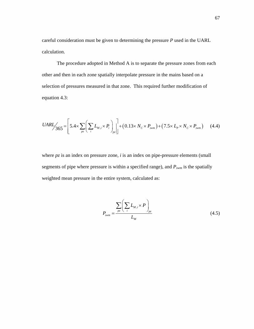
67

careful consideration must be given to determining the pressure P used in the UARL

calculation.

The procedure adopted in Method A is to separate the pressure zones from each

other and then in each zone spatially interpolate pressure in the mains based on a

selection of pressures measured in that zone. This required further modification of

equation 4.3:

( ) ( ),5.4 0.13 7.5365 M i i C swm P C swmpz i pz

UARL L P N P L N P⎡ ⎤⎛ ⎞= × × + × × + × × ×⎢ ⎥⎜ ⎟

⎝ ⎠⎢ ⎥⎣ ⎦∑ ∑ (4.4)

where pz is an index on pressure zone, i is an index on pipe-pressure elements (small

segments of pipe where pressure is within a specified range), and Pswm is the spatially

weighted mean pressure in the entire system, calculated as:

,M ipz i pz

swmM

L PP

L

⎛ ⎞×⎜ ⎟⎝ ⎠

=∑ ∑

(4.5)

68

This approach seeks to increase accuracy by mapping the interpolated system

pressure surface onto the pipe locations to find the spatially weighted mean pressure.

While detailed maps of mains were used in the audit, no data was collected on the

location of service connections, and no mapping or interpolation was performed on

service connection lines. Thus, it is assumed that spatial density of service connections

in the system is proportional to density of mains, and the spatially weighted mean

pressure is applicable to mains and service connections alike.

The pressure points used in the analysis are listed in Table 4.4 by SCADA name

with pressure zone in which each is located and the location type of the pressure point

(midpipe, pump discharge, or pump suction). Pump discharge and suction points were

included in the analysis to increase the available number of pressure points, and these

were carefully selected so that discharge and suction points balanced each other out in a

specific pressure zone to avoid biasing the mean pressure value too high or low.

Assessment of variation in hourly pressure at individual points found very little change

over the course of the year, and time-averaged annual values were used for all

calculations.

69

TABLE 4.4. Pressure Points Used In UARL Analysis

Pressure Zone Pressure Point 2004 Average Pressure (psig) Point Type P18PI140 66.3 Midpipe

SEWPI140 66.4 Midpipe 2 VALPI140 97.2 Midpipe BKHPI140 82.0 Midpipe DELPI140 74.5 Midpipe FARPI140 76.1 Midpipe H90PI140 63.0 Midpipe LOCPI140 54.8 Midpipe PHSPI140 72.6 Midpipe PYRPI140 91.4 Midpipe

3

RIVPI140 70.4 Midpipe ACMPI140 85.7 Midpipe BRPPI140 63.4 Midpipe BURPI140 58.1 Midpipe CARPI140 49.1 Midpipe FSTPI140 86.8 Midpipe LTCPI140 85.1 Midpipe MERPI140 41.6 Midpipe TRHPI140 49.8 Midpipe WILPI140 96.3 Midpipe

4

WLZPI140 75.7 Midpipe BUCPI140 75.6 Midpipe CROPI140 51.5 Midpipe EDNPI140 84.4 Midpipe PMSPI140 76.7 Midpipe SHRPI140 69.5 Midpipe

5

WESPI140 52.5 Midpipe ENPPI140 60.9 Midpipe ENSPI150 65.2 Pump Discharge JDBPI140 42.8 Pump Suction JUDPI140 111.8 Midpipe JUNPI140 91.8 Midpipe PKNPI140 93.7 Midpipe SSEPI140 44.7 Pump Discharge

6 & 9

STSPI001 74.0 Midpipe BSQPI140 80.1 Midpipe BTRPI140 105.5 Pump Discharge CALPI140 83.5 Midpipe CLNPI140 73.8 Midpipe DRHPI140 75.0 Midpipe GRNPI140 76.8 Midpipe GULPI140 62.8 Midpipe HARPI140 77.6 Midpipe HUNPI140 88.6 Midpipe INGPI140 40.0 Midpipe OAKPI140 103.1 Midpipe OCKPI140 73.4 Midpipe OKWPI140 85.1 Midpipe

7

TZLPI140 103.1 Midpipe

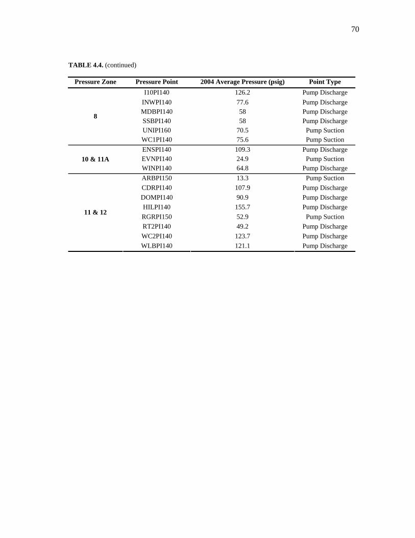
70

TABLE 4.4. (continued)

Pressure Zone Pressure Point 2004 Average Pressure (psig) Point Type I10PI140 126.2 Pump Discharge

INWPI140 77.6 Pump Discharge MDBPI140 58 Pump Discharge SSBPI140 58 Pump Discharge UNIPI160 70.5 Pump Suction

8

WC1PI140 75.6 Pump Suction ENSPI140 109.3 Pump Discharge EVNPI140 24.9 Pump Suction 10 & 11A WINPI140 64.8 Pump Discharge ARBPI150 13.3 Pump Suction CDRPI140 107.9 Pump Discharge DOMPI140 90.9 Pump Discharge HILPI140 155.7 Pump Discharge RGRPI150 52.9 Pump Suction RT2PI140 49.2 Pump Discharge WC2PI140 123.7 Pump Discharge

11 & 12

WLBPI140 121.1 Pump Discharge

71

Fig. 4.1. Map of pressure zones, pressure points, and water mains used in UARL analysis.

It was necessary to combine three pairs of pressure zones for various reasons.

Pressure zone six had only one pump suction point available, so it was combined with

zone nine. The location of points in zones 10, 11, and 12, combined with the

geographical shape of these zones caused difficulties for the spatial interpolation routine

in the GIS software. Thus, zones 10 and 11A were combined, and zones 11 and 12 were

combined. Although these changes likely introduce some small error in the calculations,

it is expected to be negligible as the length of mains in these zones is about ten percent

72

of the total for the system. A map of the final set of pressure zones and pressure points

is shown in Fig. 4.1.

In each pressure zone, average pressure was spatially interpolated on a small-cell

grid using an inverse distance weighting (IDW) algorithm in GIS. Pressure within each

zone was interpolated using only the listed pressure points within the zone. The grid of

continuously valued pressures was then reclassified to values incremented by two psig.

This step was necessary to accommodate later spatial analysis functions in the GIS. As

an example of what this step did, a specific point in the distribution system might have

an interpolated pressure of 55.7 psig based upon nearby pressure points. The grid cell

over this point would have had its pressure value reclassified to 56 psig. A nearby point

having interpolated pressure of 54.8 psig would have its pressure value reclassified to 54

psig. The reclassified pressures were then mapped onto water mains in the pressure

zone. This step produced a large set of segments of water main in each zone, where each

segment had finite length and a constant pressure along that length. Each zone’s mapped

main-pressure segments were then tabulated and totaled to produce the lengths of main

in that zone at each possible value of pressure from 0 to 156 psig in increments of two

psig. Then, the products of length and pressure were summed in each zone to produce

the term ,M i ii pz

L P⎛ ⎞×⎜ ⎟⎝ ⎠∑ needed in equation 4.4 above. This process is illustrated

schematically for pressure zone three in Fig. 4.2. The computed zonal values of total

main length, pressure-main length product, and weighted pressure (i.e., pressure-length

product divided by total main length) are given in Table 4.5 for all zones.

73

#

#

#

#

#

#

#

#

PHSPI140

PYRPI140

FARPI140

BKHPI140

LOCPI140

DELPI140

RIVPI140

H90PI140

0 1 2 3 4 5 Miles

N

Mains (shaded by mapped pressure in psi)

50 - 5455 - 5859 - 6263 - 6869 - 7475 - 7879 - 8283 - 88

PZ3 Boundary

#

#

#

#

#

#

#

#

PHSPI140

PYRPI140

FARPI140

BKHPI140

LOCPI140

DELPI140

RIVPI140

H90PI140

0 1 2 3 4 5 Miles

N

Interpolated Pressure (psi)50 - 5454 - 5959 - 6363 - 6868 - 7373 - 7777 - 8282 - 8686 - 91

#

#

#

#

#

#

#

#

PHSPI140

PYRPI140

FARPI140

BKHPI140

LOCPI140

DELPI140

RIVPI140

H90PI140

0 1 2 3 4 5 Miles

N

Reclassified Pressure (psi)50, 5254, 5656, 5860, 6264, 6668, 7072, 7476, 7880, 8284, 8688

PZ3 Water Mains

Segment LENGTH PRESSURE L x P(ft) (psi) (ft*psi)

1 444 76 33730.62 1046 76 79533.63 33 56 1861.94 184 66 12149.3↓ ↓ ↓ ↓

21846 127 74 9371.121847 13 74 955.021848 10 74 746.621849 7 74 492.2

∑ L = 4,918,008 ft∑ L = 931.44 mi

∑ L x P = 344,761,456 ft*psi∑ L x P = 65,296 mi*psi

Pressure Zone 3

Fig. 4.2. Spatial analysis and calculation of the product of main length and system pressure for pressure zone 3.

The number of service connections in the SAWS distribution system NC was

assumed to be equal to 315,000, the number of system customers stated in the FY2004

SAWS Annual Report. The length and exact location of individual service lines were

not obtained. It was assumed that service line density was directly correlated with main

density in the pressure zones.

(a) Static pressure IDW interpolated to continuous values

(b) Pressure values reclassified to 2 psig increments with mains

(c) Reclassified pressure values mapped on to main segments

(d) Tabular calculation of main segment length-pressure products and zonal sum

74

TABLE 4.5. Zonal And Total Values Of Main Length, Main Length-Pressure Product, And Weighted Pressure

Pressure Zone

Length of Mains (mi)

Main Length x Pressure (mi·psig)

Weighted Mean Pressure (psig)

2 172 13,750 79.7 3 931 65,296 70.1 4 1,199 83,881 70.0 5 485 37,915 78.2

6 & 9 299 23,017 77.0 7 864 67,139 77.7 8 255 20,376 80.0

10 & 11A 69 2,986 43.4 11 & 12 106 10,408 98.5

Total System 4,380 324,767 74.2

Average length of service lines was estimated at 50 feet and varied between 25

and 75 feet to understand the sensitivity of the final UARL value to this parameter. If

average service line length is outside of this range, further calculations should be

performed to revise the UARL calculation.

Filling in numerical values in equation 4.4, the final UARL calculation is thus:

( ) ( ) ( ) ( ) ( )505.4 324,767 0.13 315,000 74.2 7.5 315,000 74.2365 5280UARL ⎡ ⎤⎛ ⎞= × + × × + × × ×⎡ ⎤ ⎡ ⎤ ⎜ ⎟⎢ ⎥⎣ ⎦ ⎣ ⎦ ⎝ ⎠⎣ ⎦

(4.6)

This yields 6.452 million gallons per day or 2.355 billion gallons per year. This value

represents 4.4% of the system input of 52.965 billion gallons per year determined in

section 4.1.

As mentioned above, the average service line length was assumed to be 50 feet.

To test sensitivity of the UARL value to this parameter, UARL was computed for

75

average service line lengths of 25 and 75 feet. The corresponding UARL values were

2.051 and 2.657 billion gallons per year, respectively, representing ±12.9% of the

baseline UARL value. Thus, while some sensitivity exists to the assumed average

service line length, the baseline UARL value of 2.355 billion gallons per year can be

used with some confidence.

4.3.3. UARL Method B: Database Analysis Including Individual Pressure Zones

Method B is a somewhat simplified set of procedures compared to Method A in

that it does not require further use of GIS software and relies upon past GIS analysis for

main length totals in the individual pressure zones. It does preserve the separation of the

pressure zones in intermediate calculations. However, the main length-pressure product

is calculated using a simple arithmetic mean of the pressure points in the zone rather

than the spatially weighted mean pressure used in Method A. In the remainder of

section 4.2.3, Method B concepts and mathematical calculations will be presented. Also,

a step-by-step procedure for using Method B is included in Appendix A of this thesis.

76

The Method A UARL equation above (equation 4.4) is now re-written as:

( ) ( ) ( ),5.4 0.13 7.5365 M pz pz C sys P C syspz

UARL L P N P L N P⎡ ⎤

= × ⋅ + × × + × × ×⎢ ⎥⎣ ⎦

∑ (4.7)

where LM,pz is the length of mains in a single pressure zone, pzP is the arithmetic mean of

average annual pressure of the pressure points within a single pressure zone, pz is an

index on pressure zone, and sysP is the system average pressure computed as:

( ),M pz pzpz

sysM

L PP

L

×=∑

(4.8)

where LM is total length of mains in the system. All definitions of pressure zones and

pressure points remain as in Method A (see Table 4.4). Calculations for main length-

pressure products and system average pressure are shown in Table 4.6.

77

TABLE 4.6. Zonal, Total Main Length, And Pressure Calculations

Pressure Zone Main Length, LM,pz (mi)

Zonal Mean Pressure, pzP (psig)

LM,pz x pzP (psig·mi)

2 172 81.8 14,112 3 931 73.0 67,975 4 1,199 69.2 82,901 5 485 68.3 33,151

6 & 9 299 73.1 21,847 7 864 80.6 69,666 8 255 77.7 19,769

10 & 11A 69 66.3 4,561 11 & 12 106 89.3 9441

System Total 4,380 73.9 323,423 Table 4.6 can be directly compared to Table 4.5 to see the differences in

calculated values introduced by the simplifying assumptions of Method B. Several

zones see very small changes in mean pressure. Generally these zones had very small

differences in average pressure among the zone’s included pressure points or the spatial

density of mains was highly correlated with the density of pressure points. A few zones

have large differences in mean pressure, notably 5, 10 & 11A and 11 & 12. Zone 5 has a

very uneven geographical distribution of pressure points compared to main locations.

The latter two zones had no midpipe pressure points and uneven main locations.

Fortunately, the respective changes appear to cancel each other out with a very small

change in the system mean pressure (-0.3 psig).

78

Assumptions regarding service connections and service line lengths remain

unchanged from Method A. The Method B UARL calculation is thus:

( ) ( ) ( )( ) ( ) ( )505.4 323, 423 0.13 315,000 73.9 7.5 315,000 73.9365 5280UARL ⎛ ⎞⎛ ⎞= × + × × + × × ×⎡ ⎤ ⎜ ⎟⎜ ⎟⎣ ⎦ ⎝ ⎠⎝ ⎠

(4.9)

Equation 4.9 yields 6.426 million gallons per day or 2.345 billion gallons per year.

The Method B value is 0.4% less than that of Method A. This difference is

extremely small and appears to justify the simplifying assumptions used in Method B.

However, it should be remembered that several pressure zones had significant changes in

mean pressure values. As the SAWS distribution system expands (especially in pressure

zones 10, 11, and 12), careful consideration should be given to periodically revising the

GIS analysis and comparing to the simplified values of Method B.

4.3.4. UARL Method C: Database Analysis without Pressure Zones

Method C is the most simplified set of procedures compared to the two previous

methods. It does not require any use of GIS software, and it does not preserve the

separation of the pressure zones in intermediate calculations. System mean pressure is a

simple arithmetic mean of the 66 pressure points given in Table 4.4.

79

The Method A UARL equation above (equation 4.4) is now re-written as:

( ) ( )5.4 0.13 7.5365 M C P CUARL L P N P L N P⎡ ⎤= × × + × × + × × ×⎣ ⎦ (4.10)

where P is the simple arithmetic mean of all 66 pressure points. This mean for 2004 is

76.0 psig. All other values are as previously discussed. The Method C UARL

calculation is thus:

( ) ( ) ( ) ( )( ) ( ) ( )505.4 4,380 76.0 0.13 315,000 76.0 7.5 315,000 76.0365 5280UARL ⎛ ⎞⎛ ⎞= × × + × × + × × ×⎡ ⎤ ⎜ ⎟⎜ ⎟⎣ ⎦ ⎝ ⎠⎝ ⎠

(4.11)

Equation 4.11 yields a UARL value of 6.612 million gallons per day or 2.414 billion

gallons per year. This represents a change of +2.5% over the Method A value. As

higher UARL values will lead to lower values of the Infrastructure Leakage Index (ILI),

this change is not a conservative one, although it is a small one.

4.3.5. Summary of UARL Calculations

Three methods of differing complexity have been presented for computing

unavoidable annual real losses (UARL). Results from the three methods are summarized

in Table 4.7.

80

TABLE 4.7. Summary Of UARL Calculations

Method UARL (billion gal/yr)

Change from Method A

Percentage of System Input*

A 2.355 - 4.45% B 2.345 -0.4% 4.43% C 2.414 +2.5% 4.56%

* Compared to the system input (52,965 MG) as calculated in Section 4.1.

While Method A is considered the most accurate method, the value produced by

Method B is remarkably similar and requires much less effort. However, the SAWS

system is expanding with miles of main growing by about two percent each year (based

on 2002-2004 data). Future audits should every few years re-evaluate the need for

revised spatial analysis, inclusion of more pressure points, separation of currently

combined pressure zones, etc., to ensure accuracy of the UARL value. It is believed that

Method B may be used for the next two years with reasonable accuracy. Method C may

be used if very quick results are needed, but these results should be revised when

possible by a Method A or B calculation.

4.4. DEFERRED CONSUMPTION ACCOUNTING

It is recommended that a “deferred consumption accounting” category be added

to the traditional water balance diagram (shown in Fig. 2.1). When incorporating the

SAWS aquifer storage and recovery (ASR) project into this standard water balance

model, there was no obvious category for this type of water use and supply, therefore an

updated and more adaptable water balance model was developed (shown in Fig. 4.3).

The following sub-sections detail the limitations of the “International Standard Water

81

Balance” model in the context of SAWS and then describe the applications and

operation of the improved water balance.

4.4.1. Introduction to ASR Operations

During the audit year, 2004, SAWS initiated operation of its ASR project.

Throughout the course of the year, SAWS tested the Twin Oaks ASR facility,

transmitting Edwards Aquifer water to the ASR site, injecting the water into the Carrizo-

Wilcox Aquifer, and then subsequently withdrawing water from the ASR site, and

transporting it back into the SAWS distribution system. In the operation of the ASR

project, SAWS uses its distribution system infrastructure to transport water to and from

the ASR site. In addition to withdrawing stored Edwards Aquifer water from the ASR

site, SAWS also has rights to withdraw native Carrizo-Wilcox water. Currently there are

not restrictions or capped withdrawals on the Carrizo-Wilcox Aquifer (like there is with

the Edwards Aquifer), but to be prepared for any future regulatory changes SAWS

should also properly account for the amounts of Carrizo-Wilcox water it withdraws. The

year 2004 proved to be a wet year in the area; therefore use of this facility to supply

water was not needed. In dryer years to come, it will be an important source of water

supply for SAWS. A reliable accounting method for water withdrawn from both the

Edwards and Carrizo-Wilcox aquifers at the ASR project is necessary.

82

4.4.2. ASR Departure from Standard Water Balance Accounting

Integrating the ASR project into standard water auditing procedures is a

challenging task. The basic/original model does not allow for water to be input from

regular production wells and then transmitted through the distribution system to be

stored until a later unknown date. This process does not occur on a convenient one year

time scale as the audit is intended. An improved model is needed to account for

circumstances where produced water is stored somewhere (in a surface reservoir, an

aquifer, above ground tanks, etc) until it is needed at a later date. This scenario applies

only when the distribution system is also used as the transmission system (Brumbelow et

al. 2006).

4.4.3. Improved Water Balance Accounting

Fig. 4.3 is a revised version of the International Standard Water Balance

(Lambert et al. 2000) including deferred accounting principles. New entries in this

figure are described as follows. Under conditions where water is being sent to the ASR

site, the amount of water input into the distribution system contains a portion that will be

stored at the ASR site and is best described as “deferred consumption”. Deferred

83

consumption is an authorized activity which does not produce immediate revenue

(Brumbelow et al. 2006). Under conditions where water is withdrawn from the ASR site

and supplied to the SAWS distribution system, both stored Edwards and native Carrizo-

Wilcox water is supplied to the system. This amount of water is best described as

“previously deferred and now supplied”. According to the modified water balance in

Fig. 4.3, when water is withdrawn from the ASR project it is deemed Edwards water

until the volume of cumulative input into the ASR site is reached. Then, any further

volume of water pumped from the ASR site is deemed to be Carrizo-Wilcox water. This

is a convenient and necessary accounting approach to model the behavior of the ASR

project; however, SAWS makes no effort to distinguish between the two “types” of

water being withdrawn. The volume of Carrizo-Wilcox water supplied to the

distribution system is considered to be a part of the “water newly supplied” category in

the modified water balance.

84

12

34

56

Wat

er D

efer

red

Def

erre

d C

onsu

mpt

ion

Unb

illed

Def

erre

d C

onsu

mpt

ion

Def

erre

d R

even

ue

Wat

er

Res

iden

tial

Apa

rtmen

t

Com

mer

cial

Indu

stria

l

City

of S

an A

nton

io

Fire

Hyd

rant

s

Unb

illed

Unm

eter

ed

Con

sum

ptio

nLi

ne F

lush

ing

Bille

d E

xpor

ted

Res

iden

tial

Non

-Res

iden

tial

SA

WS

Met

ered

Use

Fire

Hyd

rant

s

Ass

ignm

ent L

eaks

Sur

vey

Leak

s

AS

R S

yste

m T

estin

g

Leak

age

and

Ove

rflow

s at

S

tora

ges

7

Bille

d E

xpor

ted

Wat

er

Cus

tom

er M

eter

ing

Inac

cura

cies

Bille

d M

eter

ed

Con

sum

ptio

n

Unb

illed

Def

erre

d W

ater

Una

utho

rized

Con

sum

ptio

n

Bille

d U

nmet

ered

Con

sum

ptio

n

Billi

ng A

djus

tmen

ts

Aut

horiz

ed

Con

sum

ptio

n

Unb

illed

Auth

oriz

ed

Con

sum

ptio

n

Wat

er L

osse

s

Rea

l Los

ses

Non

reve

nue

Wat

er

Bille

d Au

thor

ized

C

onsu

mpt

ion

Rev

enue

Wat

er

App

aren

t Lo

sses

Sys

tem

Inpu

t

Trin

ity A

quife

r

Wat

er S

uppl

ied

Wat

er E

xpor

ted

Edw

ards

Aqu

ifer

New

ly S

uppl

ied

Und

ocum

ente

d R

eal L

osse

s

Unb

illed

Met

ered

Con

sum

ptio

n

UA

RL

Doc

umen

ted

and

Qua

ntifi

able

Rea

l Lo

sses

Edw

ards

A

quife

r, Pr

evio

usly

Def

erre

d &

Now

Sup

plie

d

Nat

ive

Car

rizo-

Wilc

oxW

ater

Wat

er C

omin

g Fr

om A

SR

Wat

er S

ent

To A

SR

Fi

g. 4

.3.

Sing

le y

ear d

istri

butio

n sy

stem

wat

er b

alan

ce (B

rum

belo

w e

t al.

2006

).

85

Fig. 4.4 is a representation of accounting principles behind the on-going

operation of the ASR site, not limited to the one-year audit timetable due to the presence

of “carryover” quantities being assessed. This schematic depicts the previous discussion

in symbolic terms where both Edwards and Carrizo-Wilcox Aquifer water is present at

the ASR facility. During periods of water withdrawal (recovery) from this site, first any

positive accounting credits of Edwards Aquifer water are used. (The term accounting

credit is used to identify and track the volume of Edwards Aquifer water stored at the

ASR site over time.) When the positive accounting credits of Edwards Aquifer water are

used up from storage, any additional volumes of water withdrawn from the ASR site are

counted as native Carrizo-Wilcox Aquifer water. This figure also includes carry-over

quantities from year to year to account for cumulative storage of Edwards Aquifer water.

When the ASR project is in recovery mode and supplying water to the distribution

system, any water introduced to the system is first subtracted from available stored

Edwards Aquifer water according to quantities assessed in Fig. 4.4 and then introduced

into that specific year’s water balance as Edwards Aquifer, Previously Deferred and

Now Supplied. The ASR site is monitored by a SCADA system independent of the

SAWS distribution system, so it is possible to accurately and comprehensively account

for all water volumes represented in Figs. 4.3 and 4.4.

86

Fig. 4.4. Single year stored water balance with carryover quantities (Brumbelow et al. 2006).

4.5. ASSESSING METER ACCURACY

Metering water use at the customer end is an important method of enforcing

water accountability. Therefore, one of the most critical tasks in an IWA water loss

audit is quantifying the accuracy of meters in the utility system. This task is essential to

successful utility operations because these customer meters are a significant source of

income for the utility. If these customer meters are consistently under-registering, then a

larger amount of water reaches the end user than the meter measures. This is a source of

lost income for the utility and its cost per unit of water “lost” is valued at the consumer

water fee. Conversely, meters can also over-register, creating dissatisfied customers

with higher water bills than are appropriate. This section describes the methodology

used in the meter accuracy analysis of SAWS for the IWA water loss audit. First, in

87

section 4.4.1, guidelines for determining meter accuracy according to the IWA audit

procedures are reviewed as well as shortcomings. Second, in section 4.4.2, details are

given on SAWS meter testing procedures as well as statistics on meter sizes, age, and

locations. Third, in section 4.4.3, the improved procedure developed for assessing meter

accuracy for SAWS is described in detail.

4.5.1. How Does Meter Accuracy Fit into the Audit Methodology?

According to the International Standard Water Balance (shown in Fig. 2.1),

Customer Metering Inaccuracies fall under the category of Apparent Losses. These

apparent losses are an important sub-category of non-revenue water. Apparent losses are

more expensive and charged at the customer retail cost of water, because they are lost at

the customer delivery point in the water system.

Section A of the IWA audit manual describes how each component of the water

balance is calculated. Calculation box A22 from the IWA manual is named “Metering

Inaccuracies Water Losses”. Many of these calculation boxes contain formulas,

definitions, or instructions for how the water balance component should be calculated.

There are no such suggested procedures for determining this component of the water

balance (Alegre et al. 2002); therefore new calculation procedures were developed,

which are described in section 4.4.3. Once the metering inaccuracy water balance

component is calculated (A22), it is needed for the following performance indicator

calculations:

• Water resource indicator 1 – Inefficiency of use of water resources.

88

• Operational indicator 23 – Apparent losses.

• Operational indicator 24 – Real losses.

• Financial indicator 37 – Non-revenue water by cost.

Although, no direction is given in the IWA auditing format, AWWA has completed

many studies on metering procedures and technology as well as formulated standards

which SAWS meter testing shop follows carefully. Estimating meter accuracy is a very

important task in the grand scheme of completing a water loss audit, and care should be

taken to correctly develop a set of procedures and assumptions according to thorough

tests and previous research studies.

4.5.2. Inventory of SAWS Meters

SAWS has an extensive meter testing program and shop. All of the following

information, in section 4.5.2, was obtained from Louis Gutierrez, Jr., the Foreman for

Meter Repair, who is in charge of operations in the SAWS meter testing shop. The

information was obtained during a site visit on March 17, 2006.

As of March 2006, there were a total of 339,343 meters throughout the system.

Meter sizes range from 5/8-inch through 12-inches in diameter. Residential meters are

sizes 5/8-inch through 3/4-inches in diameter. Meters sizes 1-inch through 2-inches are

typically used for apartments and small businesses. Commercial/industrial meters are 3-

inches through 12-inches in diameter. The standard replacement age for all small

diameter meters (5/8” through 2”) is 15 years. This is the suggested meter replacement

schedule according to AWWA Manual M6 entitled Water Meters – Selection,

89

Installation, Testing, and Maintenance and is incorporated into SAWS operating

procedures. Large diameter (3” through 12”) water meters are normally used longer

than 15 years, until they can no longer be recalibrated or repaired to perform under

acceptable accuracy ranges. The SAWS meter testing shop routinely tests all large

diameter meters in the system every 18 months. Testing of small diameter meters does

not occur over a similar routine time frame. Instead, small meters are tested for accuracy

for one of the following reasons:

• A customer calls in complaining about an abnormally high water bill.

• SAWS staff notices abnormal behavior in records, such as unusually high or low

bills or water consumption rate and believes there is a leak or the meter is at

fault.

• If a customer fails to pay their water bill, SAWS will remove their water meter

and test it in the meter shop before re-circulating it back into the field.

• Meters 15 years old are automatically removed and not tested for accuracy.

Meter tests are completed in accordance with AWWA Manual M6. High,

medium, and low flow rates are tested for each meter and the percent accuracy is

recorded. Table 4.8 shows acceptable accuracy ranges of meter flow tests for small

diameter size meters, obtained from the SAWS Meter Testing Shop. Small diameter size

meters are shop tested, therefore the flow rate and volume of water transmitted through

each meter is standardized based upon meter size. Large diameter meters are tested in

the field; therefore the flow rates and volumes used for testing are not standard and

90

therefore not displayed in the table below. The SAWS Meter Testing Shop made all

meter test records available for review and analysis.

TABLE 4.8. Parameters For Shop Testing Of Small Diameter Size Meters

Meter Size Test Test Flow Rate

(GPM) Volume (ft^3)

Acceptable Accuracy (%)

5/8" High 13 1 98.5 to 101.5 Medium 2 1 98.5 to 101.5 Low 1/4 1 90 to 101.5

3/4" High 13 1 98.5 to 101.5 Medium 2 1 98.5 to 101.5 Low 1/4 1 90 to 101.5

1" High 40 10 98.5 to 101.5 Medium 4 10 98.5 to 101.5 Low 3/4 1 95 to 101.5

1 1/2" High 80 10 98.5 to 101.5 Medium 8 10 98.5 to 101.5 Low 1 1/2 10 95 to 101.5

2" High 120 10 98.5 to 101.5 Medium 25 10 98.5 to 101.5 Low 4 10 95 to 101.5

The meters in SAWS are produced by a variety of manufacturers. Fig. 4.5 graphically

shows the distribution of meters among the different manufactures.

91

Meter Manufacturers at SAWS9%

5%

32%

53%

1%

0%

Rockwell/SensusTrident/Neptune/SchlumbergerBadgerKent/ABB/AmcoHerseyOther

Fig. 4.5. Distribution of water meters according to brand manufacturer.

4.5.3. Procedure Developed for Meter Accuracy Assessment

4.5.3.1. Data Collection

The author conducted a site visit to SAWS meter testing shop and sampled test

records. It is important to note that when sampling test records, a significant effort was

made to randomly sample records from a range of meter manufactures and to gather

records only from tests completed in 2005 and 2006. This range of two years was

selected for the following reasons.

• Recent data was more readily available.

• It encompassed the 18 month routine meter test time span for

commercial/industrial meters, ensuring that the same meter would not have more

than one test represented in the sample.

92

• By using two years of meter test data, a larger sample of records was available to

represent the whole system. This is important for the larger size meters, because

there are few of them in the system.

See Table 4.9 to view number of samples for each meter size in comparison with the

total number of meters in the system.

TABLE 4.9. Samples Of Meter Test Records Categorized According To Meter Size

Meter Meters in Meter Records

Size Service Sampled

5/8" 295,906 165 3/4" 20,631 18 1" 10,341 21

1 1/2" 6,040 9

2" 4,238 Records

disregarded* 3" 894 35 4" 711 26 6" 414 19 8" 122 16

10" 44 10

12" 2 0

Total 339,343 319 * Records were disregarded for 2-inch meters due to non-representative sample. 4.5.3.2. Data Analysis

After meter testing records were gathered, the high, medium, and low flow

accuracy information was assimilated into spreadsheet format and organized by size of

meter for easy analysis. For each division of meter size, a simple average was calculated

93

for each of the three flow categories. See Table 4.10 to view an example of the

categorized and averaged data for the sample of ten-inch meters.

TABLE 4.10. Average Accuracy Calculations For Sample Of 10-Inch Water Meters

% Accuracy Date Set Year Tested High Flow Medium Flow Low Flow Make Model

1995 2005 100 99 100 Hersey MFM-MVU 1996 2005 98 98 98 Hersey MFM-MVU 2000 2005 98 97 100 Hersey ?

? 2005 98 98 97 Rockwell Turbine 1990 2005 100 100 100 Rockwell Turbine 1987 2005 98 98 98 Rockwell Turbine 1998 2005 98 97 98 Neptune Turbine 2001 2005 99 99 100 Neptune Turbine 2000 2005 100 99 100 Hersey FM-MVR 2002 2005 99 100 100 Hersey FM-MVR

Average = 98.8 98.5 99.1

Weighted Average of Tested Meters = 98.9

Estimated Average Accuracy for all 10” Meters in System = 99.4

Once average accuracy of the meter was calculated for each of the three flow

categories, weighting factors were applied to these three percentages to estimate the

overall accuracy of each size of water meter. Bowen (1993) (cited by Yee 1999)

recommends the following formula for calculating weighted average meter accuracy.

94

In equation 4.12, AveW is the weighted average accuracy of tested meters, LFA is the

average test result flow accuracy at low flow and in accordance MFA is at medium flow

and HFA is at high flow.

)%(8.72)%(5.18)%(8.8 HFMFLFAve AAAW ++= (4.12)

In Table 4.10, the weighted average accuracy for the test sample of 10-inch water meters

was calculated as 98.9% using equation 4.12. The weighting factors described in the

cited studies (Yee 1999, Bowen 1993) of residential water use were also applied to

commercial/industrial sized meters (as shown in this example, Table 4.10). This

application of the residential weighting factors to larger meters is obviously out of the

scope of these particular studies. However, they were used because there were no other

fitting alternatives at this time.

At this point in the meter accuracy analysis, another set of assumptions were

applied to relate the accuracy tests to true field conditions for all meters in the system.

First, small diameter meters are discussed. SAWS does not routinely test these smaller

sized meters. Instead they are tested upon customer request, when SAWS staff notices

irregularities in water bills, or before sending a meter that was removed from a non-

paying customer back out to the field. This irregular testing scheme likely results in a

sample of meters biased to underreporting of customer usage when compared to the total

population of meters. As an attempt to minimize this bias, the sample of small diameter

meters tested was assumed representative of meters nearing the end of standard service

95

life, and the final estimate of meter accuracy was determined as the average of (1) the

value aggregated from the meter test records and (2) a value of 100% accuracy. This is

based on the following assumptions.

• Accuracy of new water meters decreases at a constant rate over time (Yee 1999).

• New meters placed into service are 100 percent accurate (AWWA 1999).

For the case of large diameter meters, routine testing procedures were carried out

by SAWS, so confidence in the accuracy results for this part of the analysis are greater.

As was done for small diameter meters, overall large diameter meter accuracy was

determined as the mean of (1) the test results and (2) a value of 100%. In Table 4.10, the

final estimated average accuracy for all 10-inch meters in the system is 99.4 percent.

This, second step of averaging was completed for the large diameter meters based upon

the following assumption.

• Each time the meters are routinely tested (every 18 months), if they are

determined to be outside the specified range of accuracy, they are repaired to

meet this standard or are replaced with a meter that does meet the standard.

Therefore, after each routine test, the meters are assumed to be 100 percent

accurate. This accuracy will deteriorate linearly over time until it reaches the

accuracy which the next routine test defines. Thus, the halfway point between

the test value and 100 percent is the best estimate of the representative accuracy

for all meters in the system of that particular size.

With regard to customer metering inaccuracies, the water audit is ultimately

interested in determining two things; (1) the volume of water (gallons/year) lost due to

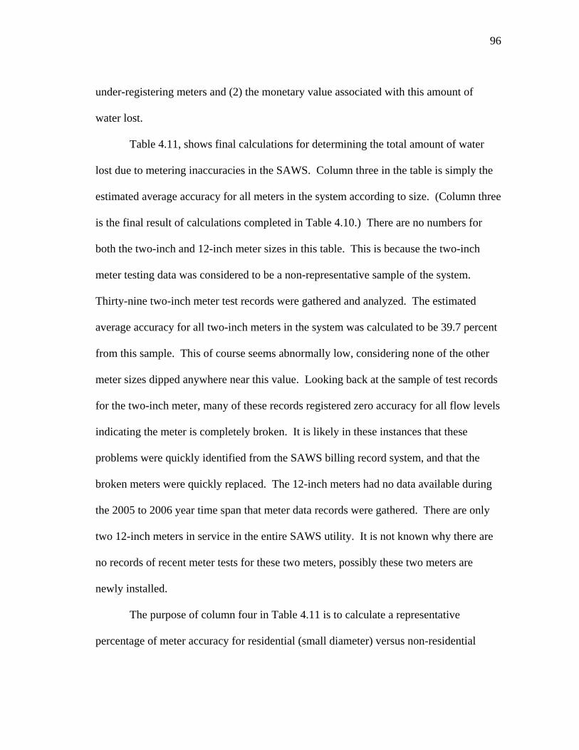
96

under-registering meters and (2) the monetary value associated with this amount of

water lost.

Table 4.11, shows final calculations for determining the total amount of water

lost due to metering inaccuracies in the SAWS. Column three in the table is simply the

estimated average accuracy for all meters in the system according to size. (Column three

is the final result of calculations completed in Table 4.10.) There are no numbers for

both the two-inch and 12-inch meter sizes in this table. This is because the two-inch

meter testing data was considered to be a non-representative sample of the system.

Thirty-nine two-inch meter test records were gathered and analyzed. The estimated

average accuracy for all two-inch meters in the system was calculated to be 39.7 percent

from this sample. This of course seems abnormally low, considering none of the other

meter sizes dipped anywhere near this value. Looking back at the sample of test records

for the two-inch meter, many of these records registered zero accuracy for all flow levels

indicating the meter is completely broken. It is likely in these instances that these

problems were quickly identified from the SAWS billing record system, and that the

broken meters were quickly replaced. The 12-inch meters had no data available during

the 2005 to 2006 year time span that meter data records were gathered. There are only

two 12-inch meters in service in the entire SAWS utility. It is not known why there are

no records of recent meter tests for these two meters, possibly these two meters are

newly installed.

The purpose of column four in Table 4.11 is to calculate a representative

percentage of meter accuracy for residential (small diameter) versus non-residential

97

(commercial/industrial large diameter) meters. This was completed by weighting each

individual meter size average accuracy (column three) according to the overall

proportion of each meter size in the system. Therefore, since there are 295,906 5/8-inch

meters of a total of 337,156 residential meters in the system, obviously the 5/8-inch size

meters weighting is much greater in proportion. Representative accuracies of 97.2% for

residential meters, and 96.5% for non-residential meters were calculated according to

equation 4.13.

231

43

85

23

2311

43

43

85

85

NNNN

NXNXNXNXAR +++

+++= (4.13)

Where RA = Weighted average accuracy for residential meters.

iX = Estimated average accuracy for each size of meter i .

iN = Number of meters in service for each size of meter i .

This same formula was utilized for non-residential meter sizes.

The volumes of water displayed in column five in Table 4.11 were determined by

an alternate member of the research project team, Dr. Cheryl Linthicum of UTSA. She

was able to determine the amount of water billed out to residential and to

commercial/industrial customers by reviewing SAWS accounting records. This volume

of water is used to determine the volume of water lost due to under-registering meters

(column six) according to equation 4.14. An important assumption at this point in the

98

discussion is that residential accounting records act in consistency with our assumption

that all meters 5/8-inch through two-inches are residential. We are counting the billing

account type “apartment” to be part of residential. In parallel, we must assume that all

commercial/industrial accounting records are consistent with meters three-inches

through 12-inches being non-residential. The City of San Antonio account type is being

incorporated into the commercial/industrial category. In reality, it is very possible that

two-inch meters could fall into either categories as well as other meters close in size.

)1()1( // icicRRerror AVAVM −+−= (4.14)

Where errorM = Apparent losses due to meter errors (gal/year).

RV = Average annual volume for residential meters (gal/year).

icV / = Average annual volume for commercial/industrial meters (gal/year).

RA = Weighted average accuracy for residential meters.

icA / = Weighted average accuracy for commercial/industrial meters (gal/year).

99

TABLE 4.11. Final Meter Analysis Showing Volume Of Losses Due To Meter Error In SAWS

Classification Meter Size

Average Accuracy for

Meter Size

Weighted Average

Accuracy for Classification

Average Annual Volume for

Classification (MG/year)

Classification Apparent Loss

(MG/year)

5/8" 97.2% 3/4" 96.8% 1" 99.9%

1 1/2" 94.3% Residential

2" Sample thrown

out.

97.2% 34,836 1,057

3" 94.9% 4" 96.3% 6" 99.4% 8" 99.3% 10" 99.4%

Non-Residential

12" No data

available.

96.5% 14,431 407.7

Total (MG/year) = 1,465

Upon conclusion of the analysis of system wide meter accuracy in the SAWS

utility, in 2004 approximately 1.465 billion gallons of water did not generate revenue

due to consistently under-registering meters, where commercial/industrial meters are

slightly less accurate than residential meters. This apparent loss of water accounts for

approximately 2.79% of the system input for the year 2004 and translates to lost revenue

of approximately $2.46 million.

100

5. SAWS WATER LOSS AUDIT RESULTS

This section presents all final results from the analysis and application of IWA

audit methodology, including recommended improvements, on the SAWS for FY2004.

First, the water balance is presented along with both quantitative and qualitative

descriptions of each pertinent category in the figure. Next, the most important

performance indicators are defined and discussed as they were applied to SAWS.

Together, these two items provide a comprehensive picture of SAWS, and gage the

utilities operational efficiency and performance during 2004. These are the end products

of an IWA audit and should be calculated every year from 2004 and on, to compare the

system’s performance and progress over time.

5.1. FINAL WATER BALANCE

Fig. 5.1 displays an adaptation of the original water balance diagram (shown in

Figure 2.1), which has been customized to fit operational characteristics unique to

SAWS. Included in this updated water balance are system output quantities (column

eight), which are either forms of consumption or losses in million gallons (MG) of

101

water. Some of these system output categories are shaded yellow. The shaded

quantities represent new additions or further refinement of the description of the water

balance category so that it is more applicable to SAWS. Also, the deferred accounting

quantities are now included in the water balance, as a means to accurately track storage

and recovery volumes of Edwards Aquifer water in the operation of the ASR project.

Last, column two in Figure 5.1 is a new addition to the water balance diagram. SAWS

produces all of its own water from a variety of sources (SAWS does not import water),

which it plans to diversify over time. The purpose of column two is to divide the system

input into volumes of water acquired from each source. In the audit year, 2004, these

potential sources included the Edwards Aquifer, the Trinity Aquifer, and the Carrizo-

Wilcox Aquifer. In future years, this column will need to be redefined to include any

new water sources. Section 5.2 explains each water balance output category (column

seven of Figure 5.1) with particular emphasis on the components discussed in section 4

of this paper (UARL methodology, deferred water concept, and meter accuracy

assessment).

102

12

34

56

8

Wat

er D

efer

red

Def

erre

d C

onsu

mpt

ion

Unb

illed

Def

erre

d C

onsu

mpt

ion

Def

erre

d R

even

ue

Wat

er18

09.5

115.

5

Res

iden

tial

2717

3.0

Apa

rtmen

t76

63.0

Com

mer

cial

1174

6.0

Indu

stria

l20

89.0

City

of S

an A

nton

io59

6.0

Fire

Hyd

rant

s13

5.4

0.0

114.

4

Unb

illed

Unm

eter

ed

Con

sum

ptio

nLi

ne F

lush

ing

54.0

82.4

3590

.3

Bille

d E

xpor

ted

4.0

Res

iden

tial

975.

3

Non

-Res

iden

tial

501.

4

SA

WS

Met

ered

Use

4.0

Fire

Hyd

rant

s4.

7

Ass

ignm

ent L

eaks

178.

3

Sur

vey

Leak

s22

.7

AS

R S

yste

m T

estin

g5.

0

Leak

age

and

Ove

rflow

s at

S

tora

ges

0.2

2345

.5

0.0

52,9

65.2

5

9,21

0

Sys

tem

Inpu

t

Trin

ity A

quife

r

Edw

ards

Aqu

ifer

New

ly S

uppl

ied

Wat

er L

osse

s

7

Bille

d E

xpor

ted

Wat

er

Cus

tom

er M

eter

ing

Inac

cura

cies

Bille

d M

eter

ed

Con

sum

ptio

n

Unb

illed

Def

erre

d W

ater

Una

utho

rized

Con

sum

ptio

n

Bille

d U

nmet

ered

Con

sum

ptio

n

Billi

ng A

djus

tmen

ts

Doc

umen

ted

and

Qua

ntifi

able

Rea

l Lo

sses

Wat

er E

xpor

ted

Aut

horiz

ed

Con

sum

ptio

n

Rea

l Los

ses

Non

reve

nue

Wat

er

Unb

illed

Aut

horiz

ed

Con

sum

ptio

n Tota

l (M

G o

f Wat

er)

Wat

er S

uppl

ied

Und

ocum

ente

d R

eal L

osse

s

Bille

d A

utho

rized

C

onsu

mpt

ion

Rev

enue

Wat

er

App

aren

t Los

ses

Unb

illed

Met

ered

Con

sum

ptio

n

UA

RL

Edw

ards

A

quife

r, Pr

evio

usly

Def

erre

d &

Now

Sup

plie

d

Nat

ive

Car

rizo-

Wilc

oxW

ater

52, 9

65.2

MG

5 M

G

49,4

02.4

MG

0 M

G

51,7

31 M

G

1,19

3 M

G

1,48

9.4

MG

2,55

1.8

MG

7,88

2.3

MG

5,16

2.1

MG

2,55

1.8

MG

7,71

3.9

MG

168.

4 M

G

49,5

17.9

MG

49,5

17.9

MG

49,6

86.3

MG

1,80

9.5

MG

1,80

9.5

MG

1,80

9.5

MG

1,80

9.5

MG

1,80

9.5

MG

115.

5 M

G

51,0

40.2

MG

Fig.

5.1

Wat

er b

alan

ce, a

dapt

ed to

SA

WS,

with

fina

lized

syst

em in

put a

nd o

utpu

t vol

umes

.

103

5.2. WATER BALANCE OUTPUT COMPONENTS

The water balance output components (column seven) are described in order

from top to bottom.

5.2.1. Unbilled Deferred Water

This category records the volume of water that is withdrawn from the Edwards

Aquifer, and then is transferred through the SAWS distribution system to the Twin Oaks

ASR site for storage in the Carrizo-Wilcox Aquifer until it is needed in the future. In

2004, 1,809.5 MG of water was stored at the ASR site (Murray et al. 2006). When

completing this water balance diagram for the next auditing period (FY2005), it is

imperative to remember that this unbilled deferred water category is not a cumulative

storage amount. The balance resets to zero at the end of the auditing period, however

the amount of deferred water left at the conclusion of the auditing period is available for

use during the next period. This water should be accounted for according to carryover

principles as in Fig. 4.4. In recovery mode for the ASR project, once this unbilled

deferred water category reaches zero and the cumulative Edwards Aquifer water stored

is also zero according to Fig. 4.4, any more water pumped from the ASR site is

considered to be native Carrizo-Wilcox Aquifer water and should be quantified as such

in column two of Fig. 5.1.

104

5.2.2. Billed Exported Water

This category quantifies the volume of water sold and exported to other water

service providers. SAWS regularly exports water to the City of Elmendorf via two six-

inch diameter metered connections, and also to East Central Water Supply Corporation

via three eight-inch diameter metered connections. (Martinez, personal communication,

2006, cited in Murray et al. 2006) As shown in Fig. 5.1, during 2004, SAWS exported

and received revenue for a total of 115.5 MG (Murray et al. 2006).

5.2.3. Billed Metered Consumption

This category quantifies the volume of water consumed by registered customers

whose meters are read monthly and then are appropriately billed. SAWS has six

different types of billing accounts; residential, apartment, commercial, industrial, City of

San Antonio, and fire hydrants. Residential, apartment, commercial, and industrial are

typical metered water uses which totaled a consumption of 48,671 MG, as shown in Fig.

5.1. The City of San Antonio account type pertains to water used by city agencies such

as the parks and recreation department, city buildings, etc. The volume of metered

consumption by the city totaled to 596 MG of water. The fire hydrant account type is an

estimate of the amount of SAWS water used at construction sites. SAWS leases fire

hydrant meters monthly to contractors, who temporarily use the fire hydrants as water

supply during construction processes. These fire hydrants are metered; therefore, each

customer is appropriately billed for their water use. Metered fire hydrant consumption

totaled to 135.5 MG for 2004 (Murray et al. 2006).

105

5.2.4. Billed Unmetered Consumption

Billed unmetered consumption quantifies the volume of water used and paid for

by customers without metered connections. These customers may be charged a flat fee

per month or the volume of water used may be estimated by an approved SAWS

procedure and then payment is made upon the estimated consumption. Potential

customers for this type of water use are city agencies such as the Parks and Recreation

Department, Department of Public Works, fire departments, or other municipal

government water uses. In the SAWS, this category of water use does not exist at this

time; therefore the assigned consumption volume in Fig. 5.1 is zero (Murray et al. 2006).

This is largely due to the fact that presently all City of San Antonio accounts are metered

(per section 5.2.3). The billed unmetered consumption category is retained in this water

balance in order to provide flexibility in case this category is needed in the future.

5.2.5. Unbilled Metered Consumption

This category quantifies the volume of water that is consumed by customers

whose meters are read, however revenue is not collected. Water use that falls into this

category within the SAWS is metered consumption for SAWS building facilities.

SAWS had 116 metered connections, which registered a total water use of 114.4 MG for

2004 (Murray et al. 2006). Of course, SAWS does not pay itself for this water use.

106

5.2.6. Unbilled Unmetered Consumption

This category quantifies the volume of water consumed without metering or

payment for its use. This type of water use occurs in the SAWS when the Operations

Department uses water for line flushing after the repair of water mains and meters. Line

flushing is performed by opening fire hydrants and releasing water in an effort to remove

any debris from the system. Since, this use is unmetered; an estimated volume

consumed for each flush is calculated with recorded information on the length of time

water was discharged, the estimated line pressure, and the size of the water main

supplying the fire hydrant. Information was not available for flushing estimates during

FY2004; therefore data for 2005 was substituted, assuming that the consumption in 2004

would be similar. SAWS estimated 4.5 MG of water was used for line flushing in June

and November of 2005. These monthly volume estimates were assumed to be

representative of the unbilled unmetered monthly consumption for 2004, totaling to a

yearly use of 54 MG. (Murray et al.)

5.2.7. Unauthorized Consumption

This category quantifies the volume of water consumed without authorization

from the water utility and, of course payment is not received for its use. This category is

often called “water theft”, which can occur through illicit service connections, bypassing

of customer meters, tampering with meters to make them more “customer friendly”, or

by installing new meters without setting up an account with the utility (Murray et al.

2006). Unauthorized consumption was estimated by collecting information from law

107

enforcement, the SAWS customer service department, and Utility Revenue Management

(a consulting firm conducting a separate project focused on revenue recovery). During

2004, twenty-eight instances of meter bypassing were discovered as well as one case of a

customer using water without being registered in the billing system. This totaled to

unauthorized consumption, non-revenue water losses, of 82.4 MG (shown in Fig. 5.1)

(Murray et al. 2006).

5.2.8. Billing Adjustments

Billing adjustments are a unique addition to the original water balance diagram

aimed at addressing an anomaly in the method SAWS uses to manage their billing

system. SAWS customer billing system also serves as a means to reimburse or wave

fees to their customers when necessary. Instead of maintaining a separate database to

account for these refunds, SAWS using the billing record database and “erases” water

use on customer accounts to provide appropriate refunds to their customers.

For example, a customer whose meter reads that 20,000 gallons of water was

used in January 2004 is owed a $25 refund for a particular reason. When refunding the

customer, SAWS subtracts an equivalent of $25 worth of water from their account for

that month. Assuming that the residential retail cost of water is $0.14 per 100 gallons,

the customer would owe $28 for their water usage that month. When applying the $25

refund, SAWS updates the customer’s billing record to read that only 2,143 gallons of

water used in January 2004 and now charges the customer $25 less on their water bill for

108

that month. This is a water accounting problem because recorded water consumption in

the SAWS billing records is less than the actual amount of water used by the customers.

Dr. Linthicum, an Associate Professor of Accounting at the University of Texas

at San Antonio, examined SAWS billing records and was able to “recover” the amounts

of water which was “erased” due to these billing procedures. It amounted to an apparent

loss of 3,590.3 MG, which is equivalent to approximately $6 million worth of refunds

(Hubbard, 2005, personal communication, as cited in Murray et al. 2006). The research

team highly recommends that SAWS modifies their current accounting practice and

separates consumption records from billing records so that this irregularity is not a

problem in the future.

5.2.9. Customer Metering Inaccuracies

Customer metering inaccuracies are defined as the discrepancy between the

amount of water actually consumed and the amount of water reportedly consumed due to

under or over registering meters. This type of error can be beneficial or detrimental to

the utility, although typically meters tend to under-register more often then over-register.

This category in the water balance is extremely important, and can pin-point a large

source of revenue loss. In a utility system which depends upon metered connections to

bill the customer, completing a thorough meter accuracy analysis is essential to

maintaining efficient operations. If the analysis concludes that meters are under-

registering significantly, it is imperative that the issue be addressed and more rigorous

procedures for meter testing and calibration be enacted.

109

Fig. 5.1 divides the customer metering inaccuracy category into five groups;

billed exported, residential, non-residential, SAWS metered use, and fire hydrants. The

consumption values (column eight) assigned to each of these five groups were calculated

first by assigning each group one of the two classifications – residential or non-

residential. In section 4.4, a methodology for meter assessment was presented and Table

4.11 displayed the final accuracy results. Residential meters were determined to be

97.2% accurate and non-residential were determined to be 96.5% accurate. Next, the

consumption registered for each of these five groups must be determined. This piece of

information is already known, and displayed in Figure 5.1 in the category billed metered

consumption. Once the billed metered consumption and meter accuracy rating for each

group is known, equation 5.1 can be applied to calculate the amount of water “lost” due

to under-registering meters in the system.

)1( AVM error −= (5.1)

Where errorM = Apparent losses due to meter errors (gal/year).

V = Billed metered consumption (gal/year).

A = Accuracy or residential or non-residential meters.

Before completing the calculation described with equation 5.1, each of the five

metering inaccuracy groups must be assigned the correct consumption value from the

110

billed metered consumption section of Fig. 5.1. The inputs into each Customer Metering

Inaccuracy group’s calculation as well as final results are as follows.

• Billed Exported apparent losses are estimated to be 4 MG. This is the loss

incurred when exporting (selling) water to the two small utilities. Recall that

SAWS transfers water their through six-inch and eight-inch metered connections

to two smaller utilities. Since these connections are of commercial size, the non-

residential meter accuracy (96.5%) was applied to the billed exported metered

consumption (115.5 MG).

• Residential apparent losses are estimated to be 975.3 MG. Residential meter

accuracy (97.2%) was applied to billed metered consumption values for both

residential (27,173 MG) and apartment (7,663 MG) accounts. Apartment

accounts were included here because they are normally operated by small

diameter (1 to 2-inches) meters.

• Non-Residential apparent losses are estimated to be 501.4 MG. Non-Residential

meter accuracy (96.5%) was applied to billed metered consumption values for

commercial (11,746 MG), industrial (2,089 MG), and City of San Antonio (596

MG) accounts. It is obvious that commercial and industrial metered connections

are large diameter and would be considered to be part of the non-residential

group. Information was not readily available regarding the size of the City of

San Antonio connections; therefore it was assumed that they are larger than two-

inches and therefore included in this group. The City of San Antonio account is

111

small when compared to the others, therefore this assumption, if proved wrong,

will not impact the final output significantly.

• SAWS Metered Use apparent losses are estimated to be 4 MG. Non-residential

meter accuracy (96.5%) was applied to the unbilled metered consumption (114.4

MG). Recall that this water was metered and used at SAWS facilities, with no

payment required. Information was not readily available regarding the size of the

meters at SAWS facilities; therefore it was assumed they are of commercial

magnitude.

• Fire Hydrant apparent losses are estimated to be 4.7 MG in Fig. 5.1, which is

slightly misleading. According to current meter testing practices, fire hydrant

meters are not tested for accuracy like customer meters. They are only tested to

ensure they are in working order. Since, there is no accuracy value to associate

with their measured consumption in 2004 (135.4 MG), the non-residential size

meter accuracy of 96.5% was applied to fire hydrant meters. Fire hydrant meters

are of a commercial size, so this is a fair assumption. It is recommended that in

the future, fire hydrant meters are tested for accuracy, so a more reliable analysis

can be made.

Metering inaccuracies totaled to 1489.4 MG of “lost” water, which is equivalent to

approximately $2.5 million for the audit year. This determination of value uses Dr.

Linthicum’s estimate for the value of water ($1678.47 per MG) delivered to customers

(Murray et al. 2006).

112

5.2.10. Documented and Quantifiable Real Losses

This category in Fig. 5.1, quantifies the amount of known physical losses from

the water system. Real (physical) losses are a form of non-revenue water loss and are

divided into four groups in the water balance diagram – assignment leaks, survey leaks,

ASR system testing, and leakage and overflows at storages. The first group, assignment

leaks, is defined as leaks reported to SAWS by a customer or area resident. After

receiving the report, SAWS will send a maintenance team out to repair the leak and then

estimate the volume of water lost. In 2004, SAWS Leak Detection/Location Program

reported an estimated 178.3 MG of water lost due to assignment leaks (Shipley 2005).

The second group, survey leaks, is defined as real losses discovered through the

efforts of the SAWS Leak Detection/Location Program. These types of leaks are not

normally on the surface, seen by the naked eye. Instead, they are found through the use

of listening devices, leak detection equipment, and the efforts of leak task forces

inspecting water lines, fire hydrants, service connections, and main valves in the system.

In 2004, SAWS staff surveyed 900.56 miles (of a total of 4380 miles) of water main in

the system, and measured an estimated 61,990 gallons per day of leaks (Shipley 2005).

This daily leakage value was multiplied by 366 days to estimate the equivalent volume

of survey leaks in 2004. This calculation process totaled an estimated 22.7 MG of

survey leaks.

The third group, ASR System Testing, is simply a specific instance where a real

loss occurred in the SAWS. During the maintenance and testing phase of the ASR

project, an estimated 5 MG of water was spilled and lost (Haby 2005, personal

113

communication, cited in Murray et al. 2006). This occurred before any Edwards Aquifer

water was stored in the ASR site; therefore the water lost was native Carrizo-Wilcox

Aquifer water. If there had been a positive credit of Edwards Aquifer water in the ASR

system at the time of the spill, then the amount of water lost would need to be subtracted

from the volume of unbilled deferred water.

The fourth group, Leakage and Overflows at Storages, is defined as the volume

of water loss occurring when an above ground storage tank overflows or a possibly a

system blow off valve opens and releases water. This type of real loss was estimated by

examining SCADA records of measured storage tank water levels (in hourly time steps),

and then comparing each tanks hourly water levels to specifications of allowable head

according to records from SAWS Production Department. Through this analysis, it was

determined that two above ground storage tanks overflowed during 2004. For each tank,

the duration in hours of the overflow condition was multiplied by the average flow rate

of water entering the tank to calculate an estimated volume of water lost due to the

overflow. (Murray et al. 2006) Table 5.1 displays a summary of these real losses, which

total to an estimated 0.2 MG in Fig. 5.1.

TABLE 5.1 Estimated Real Losses At Booster Station Storage Tanks In 2004 (after Murray et al. 2006)

SCADA Point Description Time of Overflow (hr)

Average Flowrate of Station (MG/hr)

Volume of Loss (MG)

WC2LI120 Helotes Park 2 2 0.03 0.06 UNILI120 University Tank 1 0.17 0.17

TOTAL ESTIMATED LOSS (MG) = 0.23

114

5.2.11. UARL

UARL is defined as an allowable volume of real losses from the system, which

estimates a volume of leaks that are undetectable or would be uneconomical to repair

during the year. UARL is calculated according to an empirical equation stated in the

IWA audit manual, and is sensitive to parameters such as system pressure, water main

length, and density and length of service connections. Section 4.2 of this research paper

defines and describes the UARL calculation process in great detail. UARL was

estimated to be 2,355 MG of water for 2004, as shown in Fig. 5.1.

5.2.12. Undocumented Real Losses

Undocumented real losses are defined as being equivalent to total system input

minus total system output. Typically, system input will exceed system output for a

utility indicating that there are more real losses (leaks) in their system that have not yet

been found. These extra leaks are additional to the level of UARL calculated for the

particular system. In the case of SAWS, system input was deemed to be significantly

underestimated. This “miss-balance” of the resulting water balance for SAWS in

FY2004 leads to undocumented real losses being valued at zero in the final water

balance diagram, Fig. 5.1. After system input measurement methods are hopefully

reviewed, recalibrated, and recalculated in future years, SAWS should see some value

attached to this category in the IWA water balance, even if it is a small one.

115

5.3. PERFORMANCE INDICATOR RESULTS

According to Alegre et al. (2002), a performance indicator (PI) is “a quantitative

measure of a particular aspect of the undertaking’s performance or standard of service.

It assists in the monitoring and evaluation of the efficiency and effectiveness of the

undertaking, thus simplifying an otherwise complex evaluation.” Briefly, PIs are a

simple method of comparing the efficiency of a utility with itself over time, or

comparing between utilities anywhere.

Four of the six groups of PIs were calculated for the case of the SAWS water loss

audit. The categories computed were water resources indicators, physical indicators,

operational indicators, and financial indicators. (Quality of service indicators and

personnel indicators were not included in this project.) The PIs, as calculated for

SAWS, are included in Appendix C of this thesis. Another benefit of calculating

performance indicators for various aspects of the utility system according to IWA

methodology is that during the process, each piece of data used is confidence graded to

reflect both the accuracy and reliability in the information collected. This confidence

grading is valuable when making decisions on future resource allocation and when

considering the audit results. For example, if there is little confidence in apparent loss

estimates from metering inaccuracies, the first step may be to improve the data

collection process before spending money on replacing meters, assumed to be faulty,

throughout the system. In the remainder of section 5.3, a few of the most important PIs

will be examined and compared with other utilities throughout the world. Appendix C

contains a complete list of confidence graded PIs as calculated for SAWS.

116

5.3.1. Operational Indicator 25: Infrastructure Leakage Index

This PI is the most widely reported and compared indicator for utilities

completing an IWA water loss audit. According to equation 5.2, the ILI is equal to the

following for SAWS in 2004.

Annual Real LossesILI=UARL

= 2,639.4 MG / 2,345.5 MG = 1.13 (5.2)

This performance indicator has been confidence graded “B3”, which corresponds to

reliable data with an accuracy of +/- 10%. An ILI value of one suggests that all real

losses that can feasibly be eliminated in the utility system have been located and

repaired. If this indicator is taken at face value, it would suggest that SAWS is doing a

very efficient job of locating and repairing real losses in its system. It is likely that the

SAWS Leakage Detection Program is performing their duties very well. Theoretically,

according to the ILI equation, the amount of water the utility should be able to recover

with leak detection and proper maintenance and operation is the volume of real losses

minus the volume of UARL. This would equal 293.9 MG or approximately 902 acre-

feet for the year. According to the confidence grading system assigned to this indicator,

this value may actually vary between 811 to 992 acre-feet. This amount of lost water is

minimal in comparison to the additional volume that SAWS must acquire to meet its

growing future needs.

Given the results of this particular audit, where system inputs were assessed to be

less than system outputs, the calculated ILI performance indicator is not credible. In a

117

more typical application of the IWA audit to a water utility, it would be expected that the

system input would exceed the system output and the difference between the two

volumes falls into the water balance category called undocumented real losses

(explained in section 5.11). This means that there are leaks present in the system, that

are greater than the UARL level of leakage, but these leaks have also not been located

through the use of leak detection equipment. The fact that the system input is likely

being significantly under measured in SAWS, translates to the real loss category of the

water balance also being under measured, which finally reduces the ILI incorrectly.

Until, more confidence in the system input measurements for SAWS is achieved, the

calculation of the ILI performance indicator should be viewed as preliminary.

5.3.2. Water Resources Indicator 2: Resources Availability Ratio

The purpose of this PI is to assess the percentage of overall available water

resources that the utility utilizes during the audit year. Alegre et al. (2002) encourages

use of this indicator “as a management tool, particularly in rapid growing areas or areas

subject to scarcity problems.” It seems that both of these issues are applicable to SAWS.

118

The resources availability ratio is calculated according to equation 5.3.

Water Produced 53,1012 100 100 80.9%Yearly Abstraction Capacity 65,635

MGWRMG

= × = × = (5.3)

The yearly abstraction capacity (65,634 MG) is equivalent to 234,000 acre-feet and was

determined by adding the permitted Edwards Aquifer water in 2004 to the maximum

amount allowed to pump from the Trinity Aquifer in 2004. (Abstracting water from the

Carrizo-Wilcox Aquifer was ignored in this calculation.) According to the PI, WR2,

SAWS consumed 80.9% of their available water resources. This is seen as an important

PI with respect to the SAWS, because this indicates that in 2004, a very wet year, they

did not use approximately 44,694 acre-feet of water that they had rights to abstract. If

the ASR project had come online sooner, it is possible that more of this surplus water

could have been captured and stored at the Twin Oaks ASR site for use in future years

when dry conditions reduce SAWS pumping rate from the Edwards Aquifer.

119

5.3.3. Operational Indicator 23: Apparent Losses

The purpose of operational indicator 23 is to evaluate the volume of apparent

losses per service connection in the utility system. This is a useful indicator to compare

between utility systems, in order to ascertain if apparent losses in the utility being

evaluated are normal, abnormally high, or less than average. This is useful information

for a utility in two important ways. First, by comparing to other utilities, they will know

what levels are achievable and what type of resource commitment it will take to reduce

apparent losses. Second, the utility can compare year-on-year improvements to

determine if their level of resource allocation addressing this issue is producing results.

Operational indicator 23 is defined according to equation 5.4.

service connectionApparent Losses 5157.423 0.01637

No. of Service Connections 315,000MGMGOP = = = (5.4)

120

6. CONCLUSION

6.1. ANALYSIS OF SAWS IWA AUDIT RESULTS

This section examines the direct results of the water loss audit according to IWA

principles for SAWS, as well as final values shown in the water balance, as shown in

Fig. 5.1. Section 6.1.1 compares system input to system output. Next, sections 6.1.2

and 6.1.3 analyze results from the two non-revenue water categories; apparent and real

losses. The non-revenue water category is important because it defines the aspects of a

utility where system efficiency can be improved. Last, section 6.1.4 addresses issues for

incorporating SAWS extensive water reuse/recycle program into the standard IWA

audit.

6.1.1. Inequality Between System Input and Output

Upon examination of Fig. 5.1, the first and most obvious conclusion drawn is

that the system inputs are much less than the system outputs. In fact, the water balance

indicates that approximately six billion more gallons of water was used than was

produced in SAWS for 2004, which is a disparity corresponding to about 12% of the

system input. This inequality is physically not possible, SAWS water output cannot

exceed its total input. Rather, this discrepancy must be attributed to the cumulative error

in the measurement and estimation of all quantities in the water balance. It is most likely

that the system input is significantly larger than estimated. Due to pumping restrictions

set by the Edwards Aquifer Authority on SAWS, underestimating system input is a

121

serious issue and must be carefully addressed. The TAMU research team makes the

following recommendations relevant to determination of system input volume, so that in

future audits greater confidence and accuracy in the system input volume can be

achieved.

• SAWS should re-evaluate available methods for determination of system input

volume to achieve a goal of maximum accuracy at an acceptable cost. At

present, the runtime constant flow method is used for system input volume

determination. Previous internal studies have found this method to have

accuracy of “± 3 to 5%”. However, the water balance inequality suggests that

this accuracy could be as large as ± 12%. To put this into perspective, SAWS

physical water losses are within the ± 5% range. It is difficult to have confidence

in a 5% error, when it is overshadowed by a ± 12%. Therefore, the accuracy of

the input measurement system is far less than the physical water losses in the

system. Due to its aggressive water loss control program, SAWS’s physical

water losses are now within this error range. Re-installation and/or recalibration

of flow meters at input points may allow much greater accuracy in determining

system input volume, but at some cost. A cost-benefit analysis on this issue

might be an appropriate future study.

• SAWS should conduct annual (at minimum) inspections and recalibrations for

devices needed by the preferred flow volume measurement method (runtime or

metering). At present, the runtime constant flow method for individual pumps is

the primary means with which to measure system input, but pumps are inspected

122

and runtime constants are re-calibrated only on an “as needed” basis. This

irregular schedule of inspection may allow errors to accumulate over time

leading to inaccurate system input volume determination. If the runtime constant

method is maintained as the preferred input calculation method, the “Pump

Efficiency Program” should be re-instituted as an annual inspection program (it

is likely that some energy savings would be realized as well). If flow metering is

adopted as the input calculation method, meters should be inspected and

calibrated on an annual basis.

• SAWS should consider redundancy in system input volume determination by

using both the runtime constant flow and flow metering. Future audits would

benefit by having redundant methods by which to calculate system input volume.

The presence of flow meters and runtime constants at all input points makes this

redundancy possible, but the cost of bringing both methods up to acceptable

standards of accuracy must be considered.

• SAWS should consider data entry for unmonitored stations into SCADA. At

present, 3 input stations (Bandera Road, Edison, and Lady of the Lake) are

“unmonitored” and are not represented in the system’s SCADA database.

System input from these stations is considered negligible, but finding a way to

incorporate these stations into the system’s comprehensive data will lend

completion to the water auditing process. Because of the very low volumes of

water expected to be input at these stations, this is a low priority

recommendation.

123

6.1.2. Apparent Losses

In 2004, the final water balance estimated apparent losses to be 5,157.4 MG

(15,827.5 acre-feet) of water. Apparent losses are not a physical loss of water, but rather

a missed opportunity for revenue. Resources should be allocated in controlling these

apparent losses according to the following recommendations.

• Residential meters have an estimated accuracy of 97.2%, but need to be routinely

tested for accuracy. Only a regular testing routine will provide the random

sample needed to assess meter accuracy without the biases and assumptions that

were included in this research. This is a high priority recommendation because

residential sized meters are the largest consuming group in the system; therefore

any accuracy that can be gained in this category will be a beneficial payoff with

the revenue returned to the utility.

• Non-Residential meters have an estimated accuracy of 96.5%. It is

recommended that they be recalibrated more often, so that more accuracy can be

regained and therefore the utility will be reimbursed appropriately for the water

used. This is assuming that the benefits of the recovered revenue outweigh the

cost of further meter testing.

• Fire hydrant meters should be spot tested for accuracy, so a true value (and not

just an assumption) can be used to determine apparent losses for this type of

water use. If random spot testing is done over the next year, then a better picture

of the fire hydrant meters accuracy can be assessed and it can be determined if

124

fire hydrant meters are or are not a significant source of revenue loss. For the

2004 audit, there was no information collected to be able to make this decision.

• The water use record system needs to be separate from the system used to bill

and refund customers money. This is a high priority suggestion because sifting

through billing records year after year during the IWA auditing process would be

tedious. It would be better to just go ahead and separate the two systems if

possible.

6.1.3. Real Losses

Despite the needs to better measure system input, the end result is that input and

output are close to one another (assuming zero undocumented real losses). This would

indicate that SAWS current leak detection and system maintenance programs are doing

an effective job of controlling real losses in the system. It is recommended that the

Leakage Detection/Location Program should continue at its current intensity and

funding. For 2004, recoverable real losses (not including UARL) amounted to 293.9

MG (902 acre-feet) of water (using the calculated ILI value of 1.13, which is not a fully

correct assumption). According to Fig. 3.3, SAWS will require new water assets in the

range of tens of thousands of acre-feet to meet demand projections through 2050. The

amounts of real losses not yet recovered according to this audit are minimal in

comparison to what is needed for future water supply. Therefore, at this point in time, it

is more important to spend resources on developing new water sources as opposed to

further expanding an already efficient leak detection program.

125

6.1.4. SAWS Water Reuse and Recycling Program

SAWS has an extensive water reuse and recycling program. This program has

not been mentioned or taken into account in this particular research study because it is

completely separate from the potable water distribution system audited according to

IWA methodology. The water reuse and recycling program has its own separate

SCADA monitoring system, separate infrastructure and distribution system, and supplies

recycled water for uses such as landscaping irrigation, commercial and industrial

facilities, and public fountains. Recycled water is provided at a lower fee to SAWS

customers than the traditional potable water supply. The SAWS recycled water system

has its own separate billing account procedures as well. All of the information and data

collection infrastructure is available for the water reuse and recycling program that a

separate audit could be performed on the efficiency of this system. At this point in time,

recycled water is not a valuable enough asset to motivate completing this task. SAWS is

expected to continue expansion of its water recycling program, as it allows expansion of

service with less strain on potable water supplies. As recycled water becomes a more

financially important program, its need for appropriate auditing will increase.

6.2. IWA IS AN APPROPRIATE AUDIT MODEL FOR NORTH AMERICAN

WATER UTILITIES

The IWA audit model was successfully applied in this research project to a large

North American water utility, SAWS. In any model application, new challenges will

126

arise and new circumstances will be addressed. This research project was no exception.

New and useful methodologies were developed in the study areas of:

• Defining the most accurate system input volume from multiple measurement

systems and numerous input points throughout the system.

• Incorporating deferred storage consumption principles into audit methodology.

• Calculating UARL from a system spanning many pressure zones.

• Defining a methodology for assessing meter accuracy for the system.

These model developments will aide SAWS in completing the audit in future years, as

well as any other utility that may encounter similar issues when conduction an IWA

audit.

There are multiple benefits for performing an annual IWA audit on North

American utilities. The utility is first able to measure its’ current performance by

calculating non-revenue water and performance indicators. Second, the utility can

identify problem areas within its system and formulate solutions. The utility can then

allocate resources and enact new policies to address each inadequacy. Last, in the

following year’s audit, the utility can determine if these new strategies are producing

worthwhile results. The audit must be conducted annually in order to benefit in this

manner.

127

Another significant benefit for conducting an IWA audit is that all departments

(conservation, meter testing, operations, production, finance, customer service,

compliance, planning, leak detection, and others) within the utility are forced to

communicate and work together. This benefit is especially evident for the case of large

utilities, like SAWS, where each department does not typically interact on a regular

basis. Increased communication between departments facilitates increased efficiency

and better understanding of the utilities ultimate priorities and goals.

The last significant benefit that will be discussed is the platform for international

comparison of audit results. This is useful because it is likely that somewhere in the

world, there is another utility with a similar problem, situation, configuration, etc. By

comparing each utilities performance with others, ideas can be shared on what types of

strategies work for differing problems encountered.

128

REFERENCES

Alegre, H., Hirner, W., Baptista, J.M., and Parena R. (2002). Performance Indicators for Water Supply Services, IWA Publishing: London, UK.

American Water Works Association (1999). AWWA Manual M36 Water Audits and Leak Detection, 2d ed., Denver, CO.

Beecher, J. (2002). Survey of State Agency Water Loss Reporting Practices – Final Report to the American Water Works Association, Beecher Policy Research Inc., Denver, CO.

Bexar Met Water District (2006). “Bexar Met from the Beginning.” Our History, <http://www.bexarmet.org/history1.htm> (Sep. 2, 06).

Bowen, P., Harp, J.F., Baxter, J.W., Shull, R.D., and Metcalf & Eddy (1993). “Residential Water Use Patterns”. AWWA Research Foundation, Denver, CO.

Brumbelow, K., Linthicum, C., Meyer, S., Murray, K., Nichols, D., Shelton, G., and Yosko, L. (2006). “A Comprehensive Water Audit of the San Antonio Water System.” Proc., World Environmental & Water Resources Congress 2006., ASCE, Reston, VA.

Brumbelow, K., Murray, K., and Linthicum, C. (2005). “Audit of San Antonio Water System Operations and Infrastructure using International Water Association Standards (Proposal To SAWS)”.

Collins, E.D., Havorka, S.D. (1997). “Structure Map of the San Antonio Segment of the Edwards Aquifer and Balcones Fault Zone, South-Central Texas.” Structural Framework of a Major Limestone Aquifer: Kinney, Uvalde, Medina, Bexar, Comal, and Hays Counties. Bureau of Economic Geology. Miscellaneous Map No. 38.

Eckhardt, G. (2006a). “The Trinity Aquifer.” The Edwards Aquifer Website, <http://www.edwardsaquifer.net/trinity.html> (Aug. 26, 2006).

129

Eckhardt, G. (2006b). “Aquifer Storage and Recovery.” The Edwards Aquifer Website, <http://www.edwardsaquifer.net/asr.html> (Aug. 27, 2006).

Edwards Aquifer Authority (2006a). “How Does the Edwards Aquifer Work?” <http://edwardsaquifer.org/pdfs/Education%20Resources/StudentMap2004.pdf> (Aug. 26, 2006)

Edwards Aquifer Authority (2006b). “EAA Act/Mission and Goals.” <http://edwardsaquifer.org/pages/eaaact.htm> (Aug. 26, 2006).

de Freitas, M. and Paracampos, F. (2002). “The Loss Control Program in Sao Paulo, Brazil.” Water Loss Control Manual., 465-471, The McGraw-Hill Companies, Inc.: NY.

Lambert, A., Huntington, D., and Brown, T.G. (2000). “Water Loss Management in North America: Just How Good Is It?” Proc., Workshop on Progressive Developments in Leakage and Water Loss Management, AWWA, New Orleans, LA.

Murray, K., Brumbelow, K., and Linthicum, C. (2006). Draft Report Audit of San Antonio Water System Operations and Infrastructure using International Water Association Standards, The University of Texas at San Antonio Center for Water Research, San Antonio, TX.

National Weather Service (2005a). “Monthly/Annual/Average Precipitation San Antonio, Texas (1871 – July 2006).” <http://www.srh.noaa.gov/ewx/html/cli/sat/satmonpcpn.htm> (Aug. 23, 2006)

National Weather Service (2005b). “Monthly/Annual/Average Temperature San Antonio, Texas (1885 – July 2006).” <http://www.srh.noaa.gov/ewx/html/cli/sat/satmontemp.htm> (Aug. 25, 2006)

Needham, J. (September 22, 1999). “SAWS buys farm for Edwards water storage.” San Antonio Express-News., 8b.

130

Needham, J. (February 16, 2000a). “SAWS adding 2 supply sources.” San Antonio Express-News., 1b.

Needham, J. (September 20, 2000b). “SAWS plans to tap Trinity Aquifer.” San Antonio Express-News., 7b.

Needham, J. (April 4, 2002). “SAWS revises Carrizo Policy.” San Antonio Express-News., 3B.

Pearson Education (2006). “Top 50 Cities in the US by Population and Rank.” Infoplease, <http://www.infoplease.com/ipa/A0763098.html> (Sept. 22, 2006)

Philadelphia Water Department – Water Revenue Bureau (2004). “Water Audit for Fiscal Year 2004, July 1, 2003 – June 30, 2004.” Excel Spreadsheet.

San Antonio Water System (2004). “2004 Annual Report: Water Commitment to San Antonio.” <http://www.saws.org/who_we_are/Annual_Reports/reports/2004/2004_AnnualReport.pdf> (Aug. 11, 2006).

San Antonio Water System (2006c). “About the Edwards Aquifer.” <http://www.saws.org/our_water/aquifer/aboutaquifer.shtml> (Sept. 25, 2006).

San Antonio Water System (2006a). “Conservation.” <http://www.saws.org/conservation/ > (Aug. 17, 2006).

San Antonio Water System (2006b). “History and Chronology.” <http://www.saws.org/who_we_are/chrono/chronol02.shtml> (Aug. 26, 2006).

San Antonio Water System (2004a). San Antonio Water System 2004 Stats Book. San Antonio, TX. (Prepared by the Infrastructure Planning Department and the Program Planning Division.)

131

San Antonio Water System (1998). Securing our Water Future: Water Resource Plan, San Antonio, TX.

San Antonio Water System (2005). Water Resource Plan Update 2005, San Antonio, TX.

Schindel, G.M., Hoyt, J.R., and Veni, G. (2005). “Introduction.” Proc., An Introduction to the Balcones Fault Zone Segment of the Edwards Aquifer in South-Central Texas, Edwards Aquifer Authority and George Veni and Associates, San Antonio, TX., 1-4.

Shipley, J., (2005). “Leak Detection/Location Program Summary – 2004.” SAWS Interoffice Memorandum. (Feb. 18, 2005).

Texas Water Development Board (2002). Water for Texas 2002, Austin, TX.

Texas Water Development Board (2005). Water Loss Manual, Austin, TX.

Texas Water Development Board (2006). “Instructions for Completing the 2005 Water Audit Reporting Form.” HB 3338 Water Audit Reporting Information, <http://www.twdb.state.tx.us/assistance/conservation/Municipal/Water_Audit/HB3338.asp> (Sept. 25, 2006).

Thornton, J., (2002b). “A U.S. Water Loss Case Study: The Philadelphia Experience.” In Water Loss Control Manual, G. Kunkel, ed., 443-464, McGraw-Hill, New York, NY.

Thornton, J., (2002a). “Evaluating Water Loss, Using Water Audits and Performance Indicators.” In Water Loss Control Manual, G. Kunkel, ed., 35-53, McGraw-Hill, New York, NY.

Thornton, J., (2002). “Traditional and Progressive Approaches to Water Loss: The Experiences of the United States and England.” In Water Loss Control Manual, J. Thornton and G. Kunkel, eds., 25-33, McGraw-Hill, New York, NY.

132

Water Science and Technology Board in the Committee on Privatization of Water Services in the United States (2002). Privatization of Water Services in the United States: An assessment of Issues and Experience. National Academy Press: Washington D.C.

Yee, Michael D. (1999). “Economic Analysis for Replacing Residential Meters.” American Water Works Association Journal, 91(7), 72-77.

133

APPENDIX A

UARL TUTORIAL

134

A.1. METHOD A: STEP-BY-STEP TUTORIAL This sub-section provides detailed step-by-step instructions to calculate UARL

for the SAWS according to Method A methodology.

A.1.1. Required ArcView GIS Tools & Files

ArcView GIS 3.2 was used extensively in this calculation process. It is likely

that ArcGIS 8.3 and 9 can also accomplish these tasks, but this tutorial was written to

specifically instruct the user with ArcView GIS 3.2. In order to begin the process of

determining the UARL value, the following shapefiles will need to be added to a blank

ArcView project.

• Waterline_age.shp: This is the shapefile, provided by SAWS, that maps all

water mains throughout their system. Pertinent information found in the attribute

table of this shapefile is a field containing the length of each object in feet.

• Pp.shp: This is the shapefile containing all of the pressure points currently

measured throughout the system. In addition, points have been added at booster

stations to increase the number of spatially distributed points throughout the

system.

The following polyline shapefiles of each pressure zone will be needed.

• Pz2.shp

• Pz3.shp

• Pz4.shp

135

• Pz5.shp

• Pz6&9.shp

• Pz7.shp

• Pz8.shp

• Pz10&11a.shp

• Pz11&12 .shp

The following polygon shapefiles of each pressure zone will also be needed.

• Pz2_polygon.shp

• Pz3_polygon.shp

• Pz4_polygon.shp

• Pz5_polygon.shp

• Pz6&9_polygon.shp

• Pz7_polygon.shp

• Pz8_polygon.shp

• Pz10&11a_polygon.shp

• Pz11&12_polygon.shp

A.1.2. Calculating Average System Operating Pressure

The average operating pressure of the system (in psig) must be calculated over

the course of the auditing period. Average yearly pressure values are needed for each

pressure point listed in the ArcView GIS shapefile Pp.shp. The attribute table of this

136

shapefile has three pertinent fields; Point_Name (point name), Ave_yr_pre (average

yearly pressure), and Pressure_t (pressure type). The field, point name, is where the

unique identifier for each pressure point used in the UARL calculations is listed. This

point name can be used in conjunction with the SCADA database and the program

Microsoft Access to output the measured hourly pressures at that specific point for the

auditing period.

The next field, average yearly pressure, is where the calculated average yearly

pressure for the corresponding point name should be listed. For each pressure point, use

Microsoft Access to search the SCADA database for the hourly pressures over the

course of the auditing period. Copy the pressure output table to Microsoft Excel and

then calculate the average pressure (simple mean) of the Point_average_val column for

each pressure point individually. Do this by summing all values in the column and then

divide by the number of values listed. This can be done using the COUNT function in

Excel (this allows empty cells in the database to not be included in the average). Once

the yearly average pressures have been calculated for each pressure point, enter these

average values into the attribute table of the pressure point shapefile (Pp.shp) as shown

in Fig. A.1.

137

Fig. A.1. Pressure Point attribute table (Pp.shp) in ArcView GIS 3.2, showing pertinent fields; Point_Name, Ave_yr_pre, and Pressure_type.

The last field in the attribute table, pressure type, describes the origin of the pressure

points listed. The description mid pipe refers to points listed in the SAWS SCADA data

as measured pressure points throughout their system. The descriptions discharge and

suction refer to the points that were added at booster stations to increase the number of

points spread throughout the system. Discharge points are measurements that are taken

as water is expelled from the booster stations and are accordingly higher in pressure.

Suction points are measured at the intake of the booster stations and are thus slightly

lower than normal in pressure. An effort was made to choose discharge and suction

points that are evenly distributed in pressure zones to ensure that results were not tainted

by using mostly abnormally high or low pressures.

138

In future audits, if needed, pressure points can always be added or subtracted to

this pressure point shapefile. It is encouraged to use good judgment when selecting new

points and to strive for balance between discharge and suction points in the system. If

more mid pipe pressure measurement stations are added to the system, they can always

be added to this shapefile as well and will only increase the accuracy of this process.

A.1.3. Inverse Distance Weighting Method

The Inverse Distance Weighting (IDW) Method is a process used to spatially

interpolate between data points. ArcView GIS 3.2 can quickly perform this routine. The

IDW method is used on the pressure points (Pp.shp) to create a spatially distributed

pressure across the entire SAWS service area using the previously calculated average

yearly pressure points as inputs. Pressure in a water distribution system is not spatially

distributed across the land surface; instead it is contained in the pipes. Unfortunately, no

methods or computer programs exist that are advanced enough to take into account the

pressure only traveling through the existing mains, so this IDW Method is being used to

simplify the issue. The IDW Method will be performed separately in each pressure zone

where pressures are comparable. Performing this method pressure zone by pressure

zone will help to recover some of the accuracy lost by using simplifying assumptions.

For this task, the polyline shapefiles of each pressure zone will be needed. These

files are listed in the section A.1.1. Required ArcView GIS Tools & Files of this

report. Add each of these shapefiles to an ArcView GIS map along with the pressure

point shapefile (Pp.shp). Check the theme of one of the pressure zones and the pressure

139

point shapefile. Select the pressure point shapefile by clicking on the theme again. Next

click on the ArcView GIS “Surface” menu and then select the “Interpolate Grid” option

in the sub-menu. Choose OK for the first pop-up menu that appears. In the next pop-up

menu, choose the following:

• Method = IDW

• Z Value Field = Ave_yr_pre

• Select the Nearest Neighbors option

• No. of Nearest Neighbors = 4

• Power equal to 1

• Under “Barriers” choose the pressure zone name you want to work with.

• Select the OK button.

The following figure, Fig. A.2., shows what the ArcView GIS window will look

like when performing the previously described tasks. Pressure zone three will be used

for this example and in all of the following examples in this tutorial.

140

Fig. A.2. Picture of the ArcView GIS viewport performing the IDW method.

Now, a new theme will appear on the left-hand side of the ArcView GIS

window. Check this theme to see the pressures spatially distributed across the pressure

zone. (Note, this pressure distribution will appear both outside and inside the boundaries

of the pressure zone you are using. This is acceptable; however pressure values are only

valid within the boundary of the zone.) It is wise to move forward to the next section

before repeating the IDW method for the next pressure zone. The next figure, Fig. A.3.,

shows what spatially distributed pressure zone will look like.

141

Fig. A.3. Pressure zone 3 with spatially distributed pressure point values. A.1.4. Reclassification & Conversion of Pressure Surface

The new theme just created in the above section must now be reclassified and

made permanent.

Select the “Analysis” menu and then choose the “Reclassify” option on the sub-

menu. Select the Load button from the pop-up menu. Search for the filename

reclass1.avc. This file will reclassify the surface in increments of two psig. The

following figure, Fig. A.4., shows the reclassification window with incremental pressure

classification values.

142

Fig. A.4. ArcView GIS menu showing pressure reclassification scheme.

Before choosing OK, look at the upper and lower bounds of the average yearly pressures

that have been calculated. The initial file ranges from 14 to 156 psig. Check your

average yearly pressures in the pressure point shapefile and make sure none of the values

fall outside of this range. If one does, you will have to create your own reclassification

instead of loading this file. Assuming all pressures fall within this range, continue by

selecting OK.

Another new theme will be added to your window. Check its box so that the

theme is visible. (See Fig. A.5. to see what the reclassified theme will look like.) Now

we want to make a common legend for this theme. Double click on the theme and a new

window will appear. Select the Load button from this pop-up menu, and then search for

the file named legend1.avl. Once it is found, highlight the filename and then select OK

and a new menu will pop-up. In this new window, make sure Field equals Value and the

143

All box is checked. Now choose OK. Choose APPLY on the first sub-menu and then

close the other menu as well.

Fig. A.5. Reclassified pressure surface for pressure zone 3.

The next task is to convert the theme “Reclassification of Surface from Pp.shp”

to a shapefile. First, click on the theme on the left hand side of the screen so that it is

selected. Next, choose the “Theme” menu at the top of the screen and then select

“Convert to Shapefile” on the sub-menu. A pop-up menu will appear as seen in Fig.

A.6. You are in the process of creating a new shapefile, so give it an appropriate name

(for this example Pz3_reclass, if you are working with pressure zone three) and choose a

144

directory to save it. Now select OK. The converted shapefile will be added to the

window and look similar to the one pictured in Fig. A.7.

Fig. A.6. ArcView GIS menu for converting a theme to a shapefile.

Fig. A.7. Converted shapefile showing the spatially weighted pressure surfaces for zone three.

145

This new shape (Pz3_reclass) needs to be trimmed to only the area within the

corresponding pressure zone (Pz3_polygon.shp). For this task, first, the polygon

shapefile of the pressure zone (named in section A.1.1. Required ArcView GIS Tools

& Files of this report) should be added to the window. Next, choose the “View” menu

at the top of the screen and then select “GeoProcessing Wizard” on the sub-menu. A

pop-up menu will appear as in Fig. A.8. (a) Choose the option “intersect two themes”

and then select the button Next. Choose the following options on the menu as in Fig.

A.8. (b):

• First option; select the newly converted shapefile (Pz3_reclass) as the input

theme to intersect.

• Second option; select the polygon shapefile for the corresponding pressure zone

(Pz3_polygon.shp) as the overlay theme.

• Third option; select the correct directory and select an appropriate filename

(Pz3_intersect.shp) for the new shapefile that will be created. This new theme

will be added to your window.

146

Fig. A.8. (a) GeoProcessing Wizard menu. (b) Menu option choices to perform intersection task with GeoProcessing Wizard.

147

The spatially distributed pressure shapefile trimmed to a single pressure zone will look

similar to Fig. A.9.

Fig. A.9. Spatially distributed pressures shapefile trimmed to pressure zone three. Again, continue on to the next section before beginning to work with the next pressure

zone.

A.1.5. Intersection with Water Mains

Another, ArcView GIS task that must be completed is intersecting each trimmed

reclassified and converted shapefile (Pz3_intersect.shp from the previous example) with

148

the shapefile containing the water mains (Waterline_age.shp). Add these two files to a

ArcView GIS view.

This task is accomplished by the following steps. Click on the

Waterline_age.shp theme so that it is selected. Next, choose the “select feature” button

from the toolbar along the top of the screen. While holding shift down, click and drag

around all the water lines that overlap the pressure zone you are using. Try to minimize

the region you select as much as possible because this will save processing time. (See

Fig.A.10 as an example.)

Fig. A.10. Selecting the water mains which overlap pressure zone three.

149

Next, choose the “View” menu at the top of the screen and then select

“GeoProcessing Wizard” on the sub-menu. A pop-up menu will appear. Choose the

option “intersect two themes” and then select the button Next. Choose the following

options as also seen in Fig. A.11.:

• First option, select the shapefile (Waterline_age.shp) as the input theme to

intersect. Make sure the box is checked that says “Use Selected Features Only”.

• Second option, select the output shapefile from the previous intersection task

(Pz3_intersect.shp) as the overlay theme.

• Option three, choose the correct directory and select an appropriate filename

(3_mains.shp) for the new shapefile that will be created. This new theme will be

added to your window. It will appear as in Fig. A.12.

Fig. A.11. GeoProcessing Wizard menu showing intersection between water mains and a pressure zone three.

150

Fig. A.12. ArcView GIS 3.2 window showing the resulting water main shapefile intersected with pressure zone three.

One more step is required in order to calculate the length of the water mains in

each pressure zone. This is because the previously described steps and resulting

shapefile (3_mains.shp) does not correctly determine the truncated length of water mains

which cross the boundaries of the pressure zones. In order to remedy this problem,

follow these steps in ArcView GIS. Fig. A.13 is the visual representation of following

these steps.

• Open script 3 (Script 3 is shown at the conclusion of this section (A.1.5).

151

• Manipulate your screen viewport, so that you can see both script 3 and the view

you have been using that has the water main shapefiles clipped to the single

pressure zones.

• Select the shapefile 3_mains.shp by checking its theme on the left hand side of

the view, and click on it again to make sure this is the active theme.

• Click last on the header of script 3 to make it active.

• Select the “Run” button on the toolbar across the top of the screen.

• When the program asks you if you want to “update length”, choose “Yes”.

Fig. A.13. ArcView GIS window showing the process used to calculate the truncated length of the water mains located within pressure zone three.

152

At this point, the script has successfully recalculated all the lengths of the mains

within pressure zone three, and accounted for even the mains whose lengths were

truncated as they crossed zone boundaries. This theme (3_mains.shp) is the final

product and its attribute table contains all the necessary information to calculate UARL.

Export the table from the final product shapefile (3_mains.shp) to Microsoft

Excel. This table contains several columns, two being important in this procedure. The

“Length” column lists the length of each water main in feet and the “Gridcode” column

lists the average yearly pressures of each corresponding water main. Note, there is

another column named “Shape_Length”. This column’s length does not get updated

during the previously described GIS procedures; therefore do not use its values for

subsequent calculations. Finally, this same process can be repeated with all the other

shapefiles of the water mains intersecting the other pressure zones.

Script 3, used in the calculation of the truncated lengths of the water lines is as

follows (http://support.esri.com/index.cfm?fa=downloads.geoprocessing.scripts).

' Name: View.CalculateFeatureGeometry ' ' Title: Calculates feature geometry values ' ' Topics: GeoData ' ' Description: Calculates area and perimeter for polygon themes and length ' for line themes. If the View has been projected the calculations are in ' projected meters. Otherwise the calculations are in 'native' map units. ' Modify the script to provide calculation in the current report units of ' the View. The script processes the list of active themes to calculate ' area and perimeter, or length, depending on the theme type. ' ' The script will add the fields: Area and Perimeter to polygon themes, Length ' to line themes if they do not exist. If the fields exist their values will ' be recalculated. Rerun the script if you change the projection of the view. ' ' Requires: A View with at least one active theme. You must have write access

153

' to the active theme(s). ' ' Self: ' ' Returns: ' ' Get the view and it's projection if any. ' theView = av.GetActiveDoc thePrj = theView.GetProjection if (thePrj.IsNull) then hasPrj = false else hasPrj = true end ' ' Get the list of active themes. if there aren't any, let the user know ' and exit. ' theActivethemeList = theView.GetActivethemes if (theActivethemeList.Count = 0) then MsgBox.Error("No active themes.","") Exit end ' ' Loop through the list of active themes. if you can't edit the theme ' inform the user. ' For Each thetheme in theActivethemeList theFTab = thetheme.GetFTab if (theFTab.CanEdit.Not) then MsgBox.Info("Cannot edit table for theme:"++thetheme.AsString,"") Continue end ' ' Make the FTAB editable, and find out which type of feature it is. ' theFTab.SetEditable(TRUE) theType = theFTab.FindField("shape").GetType if (theType = #FIELD_SHAPEPOLY) then ' ' if it's polygonal check for the existence of the fields "Area" and ' Perimeter. if they do not exist, create them. ' if (theFTab.FindField("Area") = nil) then theAreaField = Field.Make("Area",#FIELD_DOUBLE,16,3) theFTab.AddFields({theAreaField}) else ok = MsgBox.YesNo("Update Area?", "Calculate", true) if (ok.Not) then

154

continue end theAreaField = theFTab.FindField("Area") end if (theFTab.FindField("Perimeter") = nil) then thePerimeterField = Field.Make("Perimeter",#FIELD_DOUBLE,16,3) theFTab.AddFields({thePerimeterField}) else ok = MsgBox.YesNo("Update Perimeter?", "Calculate", true) if (ok.Not) then continue end thePerimeterField = theFTab.FindField("Perimeter") end ' ' Loop through the FTAB and find the projected area and perimeter of each ' shape and set the field values appropriately. ' theShape = theFTab.ReturnValue(theFTab.FindField("shape"),0) For Each rec in theFTab theFTab.QueryShape(rec,thePrj,theShape) theArea = theShape.ReturnArea thePerimeter = theShape.ReturnLength theFTab.SetValue(theAreaField,rec,theArea) theFTab.SetValue(thePerimeterField,rec,thePerimeter) end elseif (theType = #FIELD_SHAPELINE) then ' ' if the data source is linear, check for the existence of the ' field "Length". if it doesn't exist, create it. ' if (theFTab.FindField("Length") = nil) then theLengthField = Field.Make("Length",#FIELD_DOUBLE,16,3) theFTab.AddFields({theLengthField}) else ok = MsgBox.YesNo("Update Length?", "Calculate", true) if (ok.Not) then continue end theLengthField = theFTab.FindField("Length") end ' ' Loop through the FTAB and find the projected length of each shape and set

155

' the field values appropriately. ' theShape = theFTab.ReturnValue(theFTab.FindField("shape"),0) For Each rec in theFTab theFTab.QueryShape(rec,thePrj,theShape) theLength = theShape.ReturnLength theFTab.SetValue(theLengthField,rec,theLength) end end theFTab.SetEditable(FALSE) end

A.1.6. Calculating UARL: Water Mains

The following UARL calculation is for water mains only, and is completed one

pressure zone at a time. Mains are pipes that are accounted for in the SAWS GIS water

main shapefile. The UARL constant for mains is 5.4 gallons/miles of mains/day/psig of

pressure according to the UARL equation. To carry out the UARL calculation for this

detailed method A, add a new column to the previously described table exported into

Microsoft Excel from ArcView GIS. Title this new column UARL. Create the

following formula, equation A.1, in this column.

Shape Length daysUARL 5.4 Ave. Yearly Pressure in psi 365 ft year5280 miMains = × × × (A.1)

Sum this column to attain the total UARL value for each particular pressure

zone. Repeat procedure for remaining pressure zones and then sum all of these

156

subtotaled UARL values together to attain the total UARL values for all the water mains

in the SAWS.

A.1.7. Calculating UARL: Service Lines & Pipes between Curb Stops & Meters

Since the ArcView GIS files contain only information about the water mains and

not the service lines or underground pipes between the curb stops and customer meters,

there was not adequate information available to calculate these UARL values using the

same detailed method as with the water mains. Therefore, a couple of assumptions had

to be made in order to estimate the UARL values for these other infrastructure

components. First, these two infrastructure components are directly connected to the

water mains and therefore will have very similar pressures as the main itself. This

assumption requires an average system pressure (in psig) to be calculated. Do this

according to the following equation (Alegre et al. 2000 and Kunkel 2002):

( )365 / 5.4 / Total Miles of MainsAverage MainsP UARL= × (A.2)

The second assumption is that the average length of service connections in

SAWS is 50 feet. The following equation A.3 (Alegre et al. 2000 and Kunkel 2002)

calculates the UARL for amount of service lines in the system and for the underground

pipes which run between the curb stop and the customer meters.

( )Service Conn & Curb Stops 365 0.13 7.5Average C PUARL P N L= × × × + (A.3)

157

In the previous equation:

• UARL is calculated in units of gallons per year.

• P is the average operating pressure of the system, in units of psig as calculated

in previous equation.

• CN is the number of service connections in the system.

• PL is the average length per service connections in miles.

The final amount of UARL for this system, according to this detailed method, is

the sum of the two previous UARL infrastructure calculations. These calculations for

the 2004 auditing period produced an UARL volume of 2.355 billion gallons of water

per year.

In SAWS Comprehensive Annual Financial Report for the year 2004, they

estimate that 52.588 million gallons of water was pumped that year. In comparison with

the previous results, the UARL account for roughly 4.48% of the total pumped volume.

This UARL estimate appears reasonable.

A.2. METHOD B: STEP-BY-STEP TUTORIAL

Method B is a compromise between methods A and C. It is the preferred method

because it produces very similar results to method A while using simplifying procedures.

Using method B, the UARL volume for the 2004 auditing period only differs by 0.4 %

when compared to method A calculations. This method is much faster because it does

not require as extensive use of ArcView GIS. Also, positively, this method continues to

158

consider the impacts of the pressure zones on the SAWS and the average pressure

calculations by using a weighted average pressure according to the mileage of water

mains in each pressure zone. The following sub-sections describe the procedures for

calculating UARL according to this simplified method.

A.2.1. Calculating the Average Pressure per each Zone

See the section A.1.2. Calculating Average System Operating Pressure from

the Method A procedures to learn how to calculate AverageP for each individual pressure

zone.

A.2.2. Calculating Miles of Main per each Zone

This task involves using ArcView GIS to intersect the shapefile

“Waterline_age.shp” with each individual pressure zone, so that that the total miles of

water main per zone can be calculated. First add the shapefile “Waterline_age.shp” and

the following polygon shapefiles of each pressure zone.

• Pz2_polygon.shp

• Pz3_polygon.shp

• Pz4_polygon.shp

• Pz5_polygon.shp

• Pz6&9_polygon.shp

• Pz7_polygon.shp

• Pz8_polygon.shp

159

• Pz10&11a_polygon.shp

• Pz11&12_polygon.shp

Now, continue with the following steps. Begin by turning on the waterline

shapefile and one of the pressure zone shapefiles, in this example pressure zone two

(Pz2_polygon.shp) will be used. Choose the “select feature” button on the ArcView GIS

toolbar. While holding shift down, click and drag around all the water lines that overlap

the pressure zone you are using. Try to minimize the region you select as much as

possible because this will save processing time. Next, choose the “View” menu at the

top of the screen and then select “GeoProcessing Wizard” on the sub-menu. A pop-up

menu will appear. Choose the option “intersect two themes” and then select the button

Next. Choose the following options:

• First option, select the shapefile (Waterline_age.shp) as the input theme to

intersect. Make sure the box is checked that says “Use Selected Features Only”.

• Second option, select the output shapefile from the previous intersection task

(Pz2_polygon.shp) as the overlay theme.

• Option three, choose the correct directory and select an appropriate filename

(PZ2_mains.shp) for the new shapefile that will be created. This new theme will

be added to your window.

One more step is required in order to calculate the length of the water mains in

each pressure zone. This is because the previously described steps and resulting

160

shapefile (PZ2_mains.shp) does not correctly determine the truncated length of water

mains which cross the boundaries of the pressure zones. In order to remedy this

problem, follow the following steps in ArcView GIS 3.2.

• Open script 3.

• Manipulate your screen viewport, so that you can see both script 3 and the view

you have been using that has the water main shapefiles clipped to the single

pressure zone.

• Select the shapefile PZ2_mains.shp by checking its theme on the left hand side of

the view, and click on it again to make sure this is the active theme.

• Click last on the header of script 3 to make it active.

• Select the “Run” button on the toolbar across the top of the screen.

• When the program asks you if you want to “update length”, choose “Yes”.

At this point, the script has successfully recalculated all the lengths of the mains

within pressure zone 2, and accounted for even the mains whose lengths were truncated

as they crossed zone boundaries. This theme (PZ2_mains.shp) is the final product.

Export the attribute table from the shapefile (PZ2_mains.shp) to Microsoft Excel. This

table contains several columns, the important one being the column named “Length”.

This column lists the length of each water main in feet. Be careful to choose the

correctly named column, because there is another column named “Shape_Length” which

does not get its truncated lengths updated during the previously run ArcView GIS

161

procedure using Script 3. In Microsoft Excel, sum the “Length” column and then divide

it by 5,280 feet/mile to determine the total mileage of water mains in the pressure zone.

Repeat this same process for each pressure zone, so that the miles of main

encompassed by each pressure zone is known.

A.2.3. Calculating UARL

Use Microsoft Excel to multiply the miles of Main ( ML ) in each pressure zone

by the average pressure ( AverageP ) in the corresponding pressure zone. Then, sum these

individual values of ( ML × AverageP ) all together. Divide this summed value by the total

value of all miles of water main in the SAWS. This results in a weighted average system

pressure ( weightedP ) in units of psig.

Now, use the following equation, described in the introduction of this section, to

calculate the UARL of the system (Alegre et al. 2000 and Kunkel 2002).

5.4365 0.13 7.5Mweighted C P

C

LUARL P N LN

⎡ ⎤⎛ ⎞= × × + +⎢ ⎥⎜ ⎟

⎝ ⎠⎣ ⎦ (A.4)

Using this method produced an UARL value of 2.344 billion gallons per year.

162

APPENDIX B

SUMMARY OF SYSTEM INPUT ANALYSIS

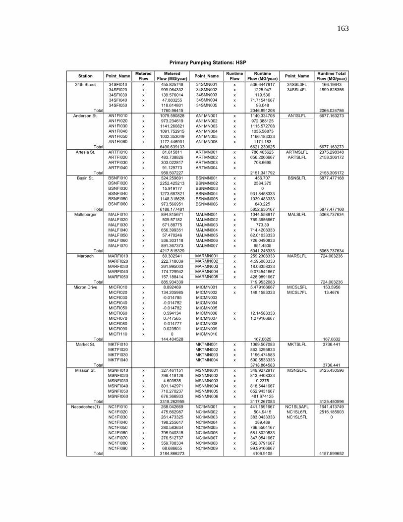
163

Metered Metered Runtime Runtime Runtime TotalFlow Flow (MG/year) Flow Flow (MG/year) Flow (MG/year)

34th Street 34SFI010 x 455.825748 34SMN001 x 536.6447917 34SSL3FL 166.1964334SFI020 x 999.064332 34SMN002 x 1225.947 34SSL4FL 1899.82835634SFI030 x 139.576014 34SMN003 x 119.53634SFI040 x 47.883255 34SMN004 x 71.7154166734SFI050 x 118.614801 34SMN005 x 93.048

Total 1760.96415 2046.891208 2066.024786Anderson St. AN1FI010 x 1079.590828 AN1MN001 x 1140.334708 AN1SLFL 6677.163273

AN1FI020 x 973.234619 AN1MN002 x 972.388125AN1FI030 x 1141.260821 AN1MN003 x 1115.572708AN1FI040 x 1091.752915 AN1MN004 x 1055.56875AN1FI050 x 1032.353049 AN1MN005 x 1166.183333AN1FI060 x 1172.446901 AN1MN006 x 1171.183

Total 6490.639133 6621.230625 6677.163273Artesia St. ARTFI010 x 81.615811 ARTMN001 x 786.465625 ARTMSLFL 2375.298348

ARTFI020 x 483.738826 ARTMN002 x 656.2066667 ARTSLFL 2158.306172ARTFI030 x 303.022817 ARTMN003 x 708.6695ARTFI040 x 91.129773 ARTMN004 x

Total 959.507227 2151.341792 2158.306172Basin St. BSNFI010 x 524.259691 BSNMN001 x 456.707 BSNSLFL 5877.477168

BSNFI020 x 2252.425213 BSNMN002 x 2584.375BSNFI030 x 15.919177 BSNMN003 x 0BSNFI040 x 1273.687821 BSNMN004 x 931.8458333BSNFI050 x 1148.318628 BSNMN005 x 1039.483333BSNFI060 x 973.566951 BSNMN006 x 840.225

Total 6188.177481 5852.636167 5877.477168Maltsberger MALFI010 x 894.815671 MALMN001 x 1044.558917 MALSLFL 5068.737634

MALFI020 x 509.57182 MALMN002 x 769.3656667MALFI030 x 671.88775 MALMN003 x 773.39MALFI040 x 656.399351 MALMN004 x 714.4208333MALFI050 x 57.470246 MALMN005 x 62.01033333MALFI060 x 536.303118 MALMN006 x 726.0490833MALFI070 x 891.367373 MALMN007 x 951.4505

Total 4217.815329 5041.245333 5068.737634Marbach MARFI010 x 69.302941 MARMN001 x 259.2308333 MARSLFL 724.003236

MARFI020 x 222.718039 MARMN002 x 4.595083333MARFI030 x 261.995003 MARMN003 x 18.06358333MARFI040 x 174.729942 MARMN004 x 9.074541667MARFI050 x 157.188414 MARMN005 x 428.9891667

Total 885.934339 719.9532083 724.003236Micron Drive MICFI010 x 8.892469 MICMN001 x 5.479166667 MICSL5FL 153.5956

MICFI020 x 134.205985 MICMN002 x 148.1583333 MICSL7FL 13.4676MICFI030 x -0.014785 MICMN003MICFI040 x -0.014782 MICMN004MICFI050 x -0.014782 MICMN005MICFI060 x 0.594134 MICMN006 x 12.14583333MICFI070 x 0.747565 MICMN007 x 1.279166667MICFI080 x -0.014777 MICMN008MICFI090 x 0.023501 MICMN009MICFI110 x 0 MICMN010

Total 144.404528 167.0625 167.0632Market St. MKTFI010 MKTMN001 x 1069.507083 MKTSLFL 3736.441

MKTFI020 MKTMN002 x 862.3295833MKTFI030 MKTMN003 x 1196.474583MKTFI040 MKTMN004 x 590.5533333

Total 3718.864583 3736.441Mission St. MSNFI010 x 327.461151 MSNMN001 x 349.9272917 MSNSLFL 3125.450596

MSNFI020 x 798.418128 MSNMN002 x 813.9408333MSNFI030 x 4.603535 MSNMN003 x 0.2375MSNFI040 x 801.142971 MSNMN004 x 818.5441667MSNFI050 x 710.270237 MSNMN005 x 652.9431667MSNFI060 x 676.366933 MSNMN006 x 481.674125

Total 3318.262955 3117.267083 3125.450596Nacodoches(1) NC1FI010 x 268.042669 NC1MN001 x 441.1591667 NC1SL5AFL 1641.413749

NC1FI020 x 475.662987 NC1MN002 x 504.9415 NC1SL6FL 2516.185903NC1FI030 x 261.473325 NC1MN003 x 383.0433333 NC1SL5FL 0NC1FI040 x 198.255617 NC1MN004 x 389.489NC1FI050 x 280.583634 NC1MN005 x 766.5504167NC1FI060 x 795.940315 NC1MN006 x 581.8020833NC1FI070 x 276.512737 NC1MN007 x 347.0541667NC1FI080 x 559.708334 NC1MN008 x 592.8791667NC1FI090 x 68.686655 NC1MN009 x 99.99166667

Total 3184.866273 4106.9105 4157.599652

Primary Pumping Stations: HSP

Station Point_Name Point_Name Point_Name

164

Nacodoches(2) NC2FI010 x 432.306097 NC2MN001 x 498.3966667 NC2SL9FL 1320.561303NC2FI020 x 7.904245 NC2MN002 x 0NC2FI030 x 43.637624 NC2MN003 x 39.85833333NC2FI040 x 624.83541 NC2MN004 x

Total 1108.683376 538.255 1320.561303Piper's Meadow PMSFI010 x 130.090833 PMSMN001 x 104.6745833 PMSSLFL 181.820409

PMSFI020 x 77.122319 PMSMN002 x 76.89583333Total 207.213152 181.5704167 181.820409

Randolph RANFI010 x 85.991171 RANMN001 x 132.2021667 RANSL4FL 1919.783483RANFI020 x 77.297879 RANMN002 x 118.0744583 RANSL6FL 252.583311RANFI030 x 820.208366 RANMN003 x 1135.905RANFI040 x 628.743125 RANMN004 x 762.1625

Total 1612.240541 2148.344125 2172.366794Seale Road SELFI010 x 69.302941 SELMN001 x 182.9882875 SELSLFL 589.981166

SELFI020 x 222.718039 SELMN002 x 145.50625SELFI030 x 261.995003 SELMN003 x 257.9992917SELFI040 x 174.729942 SELMN004SELFI050 x 157.188414 SELMN005

Total 885.934339 586.4938292 589.981166Turtle Creek 2 TC2FI001 TC2MN001 x 15.41979167 TC2SLFL 45.045658

TC2FI002 TC2MN002 x 27.563375TC2FI003 TC2MN003 x 2.000166667TC2FI004 TC2MN004

Total 44.98333333 45.045658Wurzbach WURFI010 x 1097.01765 WURMN001 x 860.031 WURSL5FL 2535.192588

WURFI020 x 1065.894018 WURMN002 x 1154.696667 WURSL7FL 5145.664453WURFI030 x 612.293036 WURMN003 x 505.44375WURFI040 x 1116.613774 WURMN004 x 494.415625WURFI050 x 1152.309654 WURMN005 x 539.0898333WURFI060 x 1305.825178 WURMN006 x 1755.187542WURFI070 x 893.097907 WURMN007 x 792.1675WURFI080 x 1047.844687 WURMN008 x 1526.84625

Total 8290.895904 7627.878167 7680.857041San Geronimo SGAMN001 SGASLFL 4.373288

SGAMN002Total 4.373288

S&S Hills SSHMN001 SSHSLFL 6.85571SSHMN002

Total 6.85571Concept Therapy CTIMN001 x 1.374053542 CTISLFL 2.145107

CTIMN002 x 1.572176667Total 2.946230208 2.145107

Culebra CULMN001 CULSLFL 34.21278CULMN002 SL5FLCULMN003CULMN004

Total 34.21278Trinity Aquifer Wells TRYSLFL x 1193.215929

Primary Pumping Stations: HSP (continued)

165

Metered Metered Runtime Runtime Runtime TotalFlow Flow (MG/year) Flow Flow (MG/year) Flow (MG/year)

Turtle Creek 3 TC3FI001 x 617.556688 TC3MN001 TC3SLFL 152.423881Babcock Rd. BBCFI001 x 0.012756 BBCMN001 BBCSLFL 0Barbet #1 BB1FI001 x 0.291865 BB1MN001 BB1SLFL 0Barbet #2 BB2FI001 x 541.614899 BB2MN001 BB2SLFL 447.606545Basse Rd. BSEFI001 x 0.89548 BSEMN001 BSESLFL 0Brackenridge (Well #13) B13FI001 x 218.488356 B13MN001Brackenridge (Well #14) BKGFI001 x 191.952544 BKGMN001 BKGSLFL 565.099705Dover KW2FI001 x 254.645894 KW2MN001 KW2SLFL 0Dreamhill DRMFI001 x 389.865055 DRMMN001 DRMSLFL 737.831907Stahl Road STSFI001 x 0.672984 STSMN001 STSSLFL 0Lackland City #3 LC3FI001 x 119.840396 LC3MN001 LC3SLFL 0Lackland City #6 LC6FI010 x 379.665738 LC6MN001 LC6SLFL 0Lackland City #6a LC6FI020 x 515.414476 LC6MN002 LCSLFLStapleton Park KW4FI001 x 39.921813 KW4MN001 KW4SLFL 0Lindbergh Park KW1FI001 x 41.724336 KW1MN001 KW1SLFL 25.315092Sutton SUTFI001 x 114.833663 SUTMN001 SUTSLFL 121.428508Loma Linda LLSFI001 x 331.968256 LLSMN001 LLSSLFL 526.663041Sunshine SUNFI001 x 141.980218 SUNMN001 SUNSLFL 149.543014Ramsey Road RAMFI001 x 2.641144 RAMMN001 0 RAMSLFL 0Klaus Road KLSFI001 x 698.537839 KLSMN001 KLSSLFL 752.05924Woodlake WLKFI001 x 177.46435 WLKMN001 WLKSLFL 76.683818West Avenue WSTFI001 x 5.407793 WSTMN001 WSTSLFL 0Walzem WLZFI001 x 93.930331 WLZMN001 WLZSLFL 80.575022Northwood Station NRSFI001 x 858.645637 NRSMN001 NRSSLFL 792.182273Upsom Park KW5FI001 x 46.915139 KW5MN001 KW5SLFL 0Gateway #1 GATFI001 x 0.356467 GATMN001Gateway #2 GATFI002 GATMN002 GATSLFL 112.339377Kelly Wells Total KWSLFL 395.365954

Unmonitored Stations:Bandera RoadEdisonLady of the Lake

Secondary Pumping Stations: HSP

Point_NamePoint_NameStation Point_Name

166

APPENDIX C

PERFORMANCE INDICATORS

167

TABLE C.1. Water Resources Performance Indicators*

* Some Performance Indicator calculations are not complete.

TABLE C.2. Physical Performance Indicators*

168

TABLE C.3. Operational Performance Indicators*

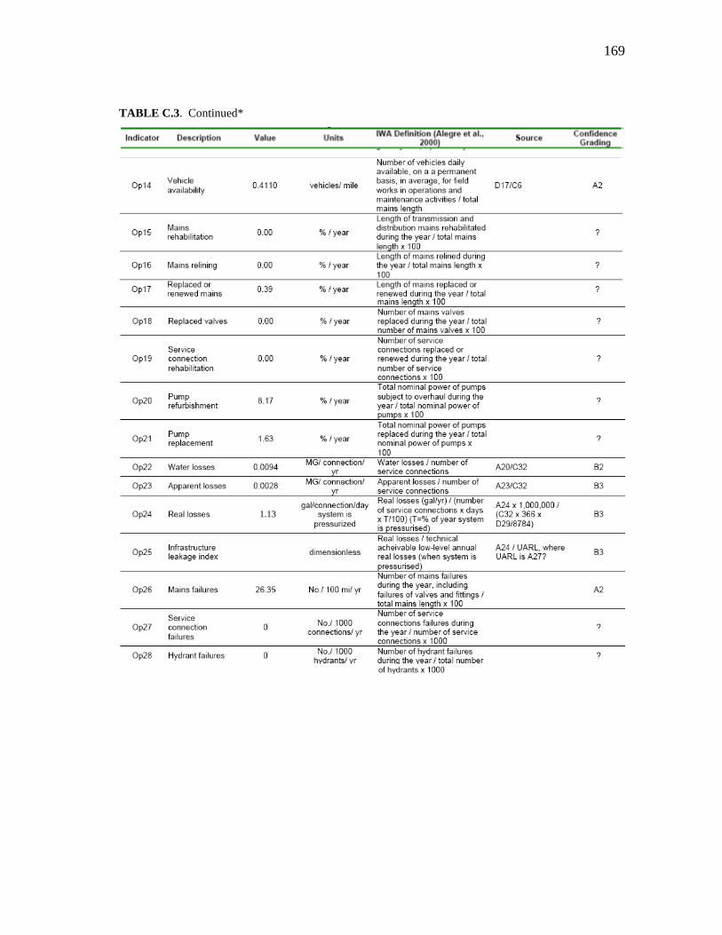
169

TABLE C.3. Continued*

1.13

170

TABLE C.3. Continued*

171

TABLE C.4. Financial Performance Indicators*

172

TABLE C.4. Continued*

173

VITA

Sarah Ruth Meyer earned a Bachelor of Science degree in civil engineering in

May 2005 from Texas A&M University. Since then, she has worked towards a Master

of Science degree also from Texas A&M University, focused in water resources

engineering.

Sarah’s graduate studies have been supported by a research assistantship funded

by San Antonio Water System, a teaching assistantship, and by award of the Texas

Section ASCE Hawley Fellowship. Throughout the course of her college career, Sarah

has interned with a couple of engineering consulting firms. These internships include

working with the hydrology and hydraulics group at Lockwood, Andrews, and Newnam

Inc. (Summer 2005 and 2006) and a land development firm, Bury + Partners, Inc.

(Summer 2004). These internship opportunities helped motivate her to pursue graduate

level studies as well as focus her learning upon engineering and management of Texas

critical water resources. Upon receipt of her Master’s Degree in December 2006, she

will be working as a consulting civil engineer with an emphasis in water resources.

Sarah Meyer can be reached at the following email and physical address:

Sarah2004@tamu.edu, PO Box 1206, La Vernia, TX 78121.