Geophysical Prospectilag, 1999,47, 85-101

Improvement to resistivity pseudosection modelling by removal of near-sudace inhomogeneity effects: application to a soil system in south Cameroon’

Michel Ritz,’ Henri R ~ b a i n , ~ Evgeni Per~ago,~ Yves A l b ~ u y , ~ Christian Camerlyn~k,~ Marc Descloitres3 and Adama Mariko6

Abstract

Near-surface inhomogeneities (NSIs) can lead to severe prob1ems”in the’ihterpietation of apparent resistivity pseudosections because their effects significantly complicate the image aspect. In order to carry out a more efficient and reliable interpretation process, tliese problematic features should be removed from field data. We describe a filtering scheme using two-sided half-Schlumberger array data. The scheme was tested on synthetic data,, generated from a simple 2D resistivity model contaminated by NSIs, and is shown to be suitable for eliminating such contaminations from apparent resistivity data. Furthermore, the original model without NSIs can be recovered satisfactorily from the inversion of filtered apparent resistivity data. The algorithm is also applied efficiently to a real data set collected at Nsimi, in southern Cameroon, along a 200-m shallow depth profile crossing a complex transitional zone. For this case, the filtering scheme provides accurate structural and behavioural interpretations of both the geometry of the major soil constituents and the groundwater partitioning.

‘Introduction

’Electrical resistivity methods are used for shallow prospecting in a variety of environmental, geological and hydro-geological applications. Several recent studies have paid particular attention to the determination of the geometry of the overburden terrain (Delaître 1993; Lamotte etal. 1994; Robain etal. 1995, 1996; Cherry etal. 1996). Moreover, detailed resistivity pseudosections obtained using dense multi- electrode profiling complement fractional observations obtained from pits, hand- drilling, etc.

Received February 1997, revision accepted March 1998. ORSTOM, B.P. 1386, Dakar, Senegal. ORSTOM, 32, avenue Henri Varagnat, 93143 Bondy Cedex, France.

Département de Géophysique Appliquée, Université Paris 6, 4 Place Jussieu, 75252 Cedex 05, France. Ecole NátiöGle d‘Ingénieur, B.P. 242, Bamako, Mali.

4 M ~ ~ ~ ~ ~ State University, Faculty of Geology, Department of Geophysics, 119899 Moscow, Russia.

I I

r - - O -- 1999 .- European Association of Geoscienbsts & Engineers 85

Fon as Do cumenla¡ re o KSTOiVVP

86 M. Ritz et al.

Current experience in resistivity surveys for various geological situations shows that near-surface inhomogeneities (NSIs) are quite common (IChmelevskoj and Shevnin 1994). NSIs produce strong signatures which extend far beyond their location and may thus disturb or mask signals related to deeper structures of more particular interest (Bibby and Hohmann 1993; Brune1 1994). Consequently, when deep targets are under investigation, NSI features increase the time that must be spent building models to describe such targets. The more complicated the field data are, the more time- consuming the construction of a reliable model will be. Moreover, such situations may lead to a severe misinterpretation of data if NSI features are not recognized. A solution to circumvent this problem is to remove NSI features from the measured pseudosection in order to build a simplified model in which the effects of small near-surface objects have been filtered out.

We present a filtering scheme which removes NSI effects from resistivity pseudosections (Modin etal. 1994). This scheme, based on the median polishing algorithm of Tukey (1981), is applied to both synthetic data and real data collected from a site in southern Cameroon.

Methods

Resistivity inensiirements

The electrical prospecting method consists of measuring the potential at the surface which results from a known current flowing into the ground (Van Nostrand and Cook 1966). A pair of current electrodes, A and B, and a pair of potential electrodes, M and N, are used. The apparent resistivity (pa) is given by

pa = KAVII , (1)

where I< denotes a geometric coefficient dependent upon the electrode array, AV denotes the measured potential difference and I denotes the current intensity. By expanding the current electrode array, the depth of investigation can be increased. Such a data set provides a vertical log of apparent resistivities called a vertical electrical sounding (VES). The sounding site is conventionally located at the centre between the inner electrodes. Recently developed computer-controlled multichannel resistivity meters allow tens of electrodes to be connected, of which any independent: combination of current and potential electrodes can be recorded sequentially over a short period of time. The resulting detailed apparent resistivity pseudosection corresponds to very close VESs (Barker 1992). Furthermore, the pseudosection provides a precise image with dense sampling of the resistivity distribution in the ground at a shallow depth (= O-loom).

In the field example presented below, the pole-pole array (also called the two electrodes array) was used. A pseudosection consisting of 1500 measurement points was carried out along a 200 m-long profìle. B and N were fixed and located sufficiently far away from the profile to be considered at infinity. A and M were selected from 40 in- line electrodes spaced 2 m apart (Fig. 1). The surveyed profile was swept over a period

. li-

/ ,

> ì

I

a

O 1999 European Association of Geoscientists & Engineers, Geophysical Prospec&g, 47, 85-1 O 1

Resistivity pseudosection rraodelliizg 87

- E o - 5 10- -g 20-

1

n

O 4 30 - al V) 40 - n

Fir thePS

Second part I I l I I

of four days, moving this in-line array step-by-step. The pole-pole array was chosen in view of its superior depth of investigation compared with other configurations (Roy and Apparao 1971) and also because the data produced can be converted for any other form of electrode arrangement (Beard and Tripp 1995). c

Data processing

Various programs using either inverse or forward modelling methods are available to process apparent resistivity pseudosections and to perform 2D imaging of the underlying structure (Rijo etal. 1977; Bobatchev et al. 1990a,b; Loke and Barker 1996). NSI effects may, however, complicate or, in a worst-case scenario, cause erroneous interpretations of the data. An analysis by Modin etal. (1994) of field

0 1999 European Association of Geoscientists & Engineers, Geop?zysical Prospectitzg, 47, 85-101

58 M. Ritz et al.

+ HL

+ P

COMPONENTS EXTRACTION

4 v

resistivity data from different regions showed that NSI effects may be found in more than 70% of VES curves. These distortions may be divided into two groups: P-effects, caused by NSIs near the potential electrode, and C-effects, caused by NSIs near the current electrode. In terms of alterations to the VES, P-effects shift the VES curve up or down along the apparent resistivity axes without changing the actual form of the curve (i.e. the potential electrode remains near the same NST). C-effects distort only a portion of the curve (i.e. the current electrode crosses over the NSI as the array expands). Hence NSIs influence apparent resistivity pseudosections strongly, complicating their 2D images with convoluted waved forms (P-effects) and inclined lines (C-effects).

Because P- and C-effects generate clear distortions on apparent resistivity pseudosections, they can therefore be removed using an appropriate fiter. We use a median polishing algorithm for data tables (Tukey 1981) adapted by Pervago etal. (1995). It should be noted that analogous filtering processes are commonly used in image analysis (Scollar, Weicher and Huang 1984), to filter geophysical maps (Tabbagh 1988), to prepare seismic data for noise suppression (Evans 1982) or for wave separation (Hardage 1985).

The filtering process includes three steps: extraction of components, smoothing and reconstruction (Fig. 2 ) . The process is applied to a table of apparent resistivity data logarithms, where each row corresponds to a pseudodepth and each column to a sounding site. In such a table, the effect of horizontally layered media is displayed simultaneously for all columns. I'-effects are displayed for some columns correspond- ing to NSI locations, wlvle C-effects are displayed as inclined lines descending from the

.)

, \.i

v + CAmn RAmn

Q 1999 European Association of Geoscientists & Engineers, GeoplzysicaZ Prospecting, 47, 85-1 O1

j j RmnB CmnB 4

E A m n RAmn GL SMOOTHING - p g m n B EmnB

RECONSTRUCTION -mnB P -Amn P

Resistivity pseudosection modelling 89

first row of the column next to the NSI location. Orientation to the left or to the right depends on the array type.

The process requires two-sided half-Schlumberger data (Amn and mnB). This data may be obtained directly using arrays where the B and A electrodes are each placed sufficiently far away from the other three electrodes to be considered at infinity. Pole- pole field data are also suitable but must be converted to the couple Amn and mnB data before the filtering process is applied. In such pseudosections, C-effects are only displayed on a line inclined to the right for the Amn array or on a line inclined to the left for the mnB array. Hence these distortions are well separated.

The first step in the filtering process separates the initial apparent resistivity data into four components: horizontally layered medium (HL), NSI P-effects (P), NSI C- effects (C) and all other features (R). A simple synthetic example with both matrices and images showing how the HL-, P-, C- and R-components are extracted is given in the Appendix. The second step in the process removes high-frequency variations from each component using a moving spatial average filter. These variations are basically associated with NSI and measurement noise. The width of the smoothing window may therefore be adjusted depending on the survey conditions and geological structures. From these procedures it can be seen that if NSI structures are of particular interest in the survey, the values of related P- and C-effects, corresponding to the high-frequency variations of P- and C-components that have been removed, can be estimated for each site and drawn as separate diagrams. The last step reconstructs apparent resistivity data by recombining the smoothed HL-, P-, C- and R-components. It also provides filtered Amn and mnB pseudosections, free from NSI distortions and measurement noise. These pseudosections may be interpreted either in this state or after half-summation which provides a symmetrical total-Schlumberger pseudosection.

Synthetic example

Synthetic apparent resistivity pseudosections are generated from the two flexure models shown in Fig. 3. The first model consists of a simple three-layer resistivity structure, with a slight downslope to the right (Fig. 3a). In the second model, some NSIs have been added to the uppermost layer (Fig.3b). Synthetic Amn and mnB pseudosections contaminated with NSIs are shown in Fig. 3c. They appear considerably distorted with respect to the synthetic total-Schlumberger (AmnB) pseudosection, which consists of the flexure alone (Fig. 3d). Figure 3e shows the AmnB pseudosection that was obtained by combining Amn and mnB filtered pseudosections, where the distorting influence of the NSIs has been removed. Its form is very similar to that of Fig.3d. The use of this procedure results in a clear improvement to the pattern of apparent resistivity contours.

It is convenient here to introduce the technique of 1D joint inversion of each VES, described by Bobatchev etal. (199Oa) to obtain a reliable interpretation of the filtered pseudosection. As the slopes of the layers are gradual in this example, the error made in using this procedure to estimate the depth of the interfaces at each VES location is

.

O 1999 Eurouean Association of Geoscientists & Engineers, Geo&sicd Prospecting, 47, 85-101

o c W W W

Model without NSI

(4 O I

10 m

20

Model with NSI

15 150 20 125 15 I c a a a a a o r m (b)

I

1 Forward modelling IC)

,,Amri

Forward modelling ,,mnB

(d) pAmnB 4 pAmnB 1 NSI effects removal (e)

Figures.

50

15' o m 20

NSI

2D modelling necessary 1 but overcomplicated

2D modelling not needed (cl)

W O

Synthetic example of the removal of NSI effects.

Resistivity pseudosectio?z ?~zodelli~zg 9 1

insignificant (Kunetz 1966). However, this technique gives completely erroneous results for the pseudosection witli NSI effects. Using this filtering scheme, the models estimated from synthetic data before and after filtering are shown in Figs3f and g, respectively. The difference between the two models is striking. The model before filtering shows boundaries distorted in the vicinity of the NSIs. By contrast, the model obtained after filtering gives much less perturbed structure boundaries, thus comparing favourably with the initial model.

It should be noted that the filtering of P- and C-effects cannot be carried out for a single isolated VES. An effective filtering process depends on the information provided by many closely spaced VESs acquired along a profile, using multi-electrode arrays or traditional electrical sounding techniques. For such polished data sets, 1D inversion is sufficient to obtain a reliable interpretation of ground structures that possess a simple geometry (i.e. close to tabular). For more complicated structures, such as the real field example presented below, the filtering facilitates at least the required 2D modelling.

Field data example: Nsimi site

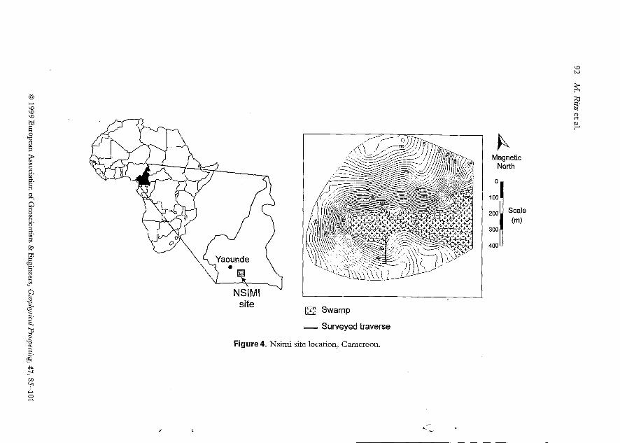
The 200-m profile presented in this example is located at the Nsimi site in the rain forest of southern Cameroon (Fig. 4). Knowledge of the subsurface structure of the site is constrained by auxillary pedological and geological data.

I Geological and pedological'settings

The parent lithology for soils in the area, found only in outcrops, is a leucocratic acid charnolute metamorphosed to granulite facies.

The characteristics of the soils were determined from 5 pits and 18 hand-drill logs (Fig. 5). The pits were excavated to the depth of the water table (from 1 to 12 m), whereas the deptli of the drillholes was determined by the point where the auger jammed, generally at the top of ferruginous materials found at the southern part of the profile.

The soils contained three main divisions: (1) unconsolidated topsoil, (2 ) indurated ferruginous clays and (3) saprolite. Four different horizons could be distinguished within the topsoil: dark brown clayey peat (P), pale-grey and yellow sands (S), yellow and red sandy-clays (SC) and red clays (C) . Two horizons could be identified within the ferruginous materials: soft ferruginous network (SFN) cross-cutting white, red and yellow clays, and red and yellow clays containing numerous indusated ferruginous pebbles (IFP) . Finally, there were two horizons within the saprolite: white loamy-clays (WSp) and variegated loamy clays (VSp) .

The swamp and the hillside on the site exhibit vertical successions of soil materials, P/S/WSp and C/IFP/VSp, respectively. The transitional zone, covering = 150m, is characterized by the vertical succession SC/C/SFN/VSp. Lateral variations from the swamp to the hillside are characterized by the disappearance of P from the topsoil (Fig. 5, O), the appearance of SC in the middle of S (Fig. 5, O), the appearance of SFN

O 1999 European Association of Geoscientists & Engineers, Geopkwical Prospecting, 47, 85-101

i

o CL W W W

g 5

O “r

f L

site

1 P Magnetic I North

Scale

300

400

a Swamp

- Surveyed traverse

Figure 4. Nsimi site location, Cameroon.

2- < -

@ o 690

Transitional zone 685

h

E d 680 I Q

p 675

v

C O

> a, Lu -

670

665 550 600 650 700 750 800 850 900

Distance (m)

Pedological observations Soil materials

Pit mp I ' S C SFN a WSp R

Figure 5. Cross-section of the soil system along the electrical survey line obtained from pits and hand-drilling observations. P, peat; S, sands; SC, sandy-clays; Cy clays; SFN, soft ferruginous network; IFE indurated ferruginous pebbles; WSp, white saprolite; VSp, variegated saprolite; R, rock basement; GWT, groundwater table level measured in piezometres. Numbered open and solid circles are the locations of the disappearance and appearance, respectively, of pedological materials along the cross-section from north to south.

94 M. Ritz et al.

between SC and S (Fig. 5, O), the disappearance of S at the topsoil and at the bottom of SFN (Fig.5, O), the appearance of C between SC and SFN (Fig.5, O ) , the disappearance of SC at the topsoil (Fig. 5, O), the appearance of IFP at the top of SFN (Fig. 5, O) and finally the disappearance of SFN at the top of IFP (Fig. 5, @I). No transition could be observed between WSp and VSp on this cross-section because these two saprolites are separated by a basement outcrop located to the north of the transitional zone.

The groundwater table (GWT) rises to the surface in the swamp, reaches the bottom of SFN in the transitional zone and then descends through VSp to the south leaving = 5 m of this horizon top unsaturated at the most southern pit.

NSI removal and 2 0 forward modelli~g

In order to use the filtering algorithm presented above, pole-pole field data collected at Nsimi were converted into two Amn and mnB pseudosections.

Figure 6 shows the three steps of NSI removal from the resistivity pseudosections. After reconstruction, the pseudosections showed little irregularity with respect to the original data. However, the filtered total-Schlumberger pseudosection (Fig. 7a), obtained by combining the filtered Amn and mnB pseudosections, still exhibits strong lateral effects that indicate the presence of a complex structure. 1D modelling is inadequate to interpret such a pseudosection reliably. Hence a 2D forward modelling using a surface integral procedure was performed (IPI-2D software, Bobatchev et al. 1990b). 1D interpretations were nevertheless used to construct an initial model. This model was then adjusted until a fit with the filtered Schlumberger apparent resistivity pseudosection was achieved. The computed pseudosection obtained from the optimized 2D model is shown in Fig. 7b.

Structural features

The final 2D model (Fig. 8) obtained by forward modelling shows that the elevated values of apparent resistivity probably represent the rise of the resistive basement near the surface beneath sites 620-670. It also reveals a large contrast in resistivity between the southern and the northern sides of the traverse at depths shallower than 4m. In detail, the model highlights three different sectors: o A northern area (sites 580-620), located in the swampy zone, is characterized by thin

(less than 6 m) intermediate-resistivity (1 80-500 Qm) formations overlying a resistive basement (2000 Om). Two layers can be detected above the resistive basement. The upper layer (250 Om), the thickness of which decreases to the south, corresponds to the peat zone (P) detected in pitting. Below is a 180Qm layer, interpreted as representing the saprolite (WSp).

o A central part (sites 620-670) is characterized by the resistive basement rising to the surface. It appears as a dome-like structure. The abrupt lateral resistivity change in the basement at site 640 represents an important geological discontinuity. This

Q 1999 Eurooean Association of Geoscientists & Emineers. Geoahvsical ProsaectinP. 47. 85-1 O1

<- e.

P- FIELD DATA

COMPONENTS EXTRACTION

Figure 6. Various steps of 1 31 removal from the Nsimi field data. The top gures are the Amn and mnB apparent resistiviv pseudosections derived fiom field pole-pole data. The upper central figures are the extracted components: horizontally layered medium (a), i.e. the apparent resistivity stratification versus depth. C-effects (CA”” and C-), P-effects (P) along the profile and the residual pseudosection (R) are expressed as a percentage of initial data. The lower central figures are the smoothed components where high-frequency variations have been removed. The lowest figures are the filtered pseudosections where NSI effects are removed by recombining the smoothed components.

M. Ritz et al.

600 640 680 720 760

O U al 3 2

E 5

10

20

50

am

2700

2000

1400

1 O00

700

Pa AmnB

Distance (m)

Figure 7. Comparison between Schlumberger apparent resistivity pseudosections observed (a) and computed (b) for the final 2D resistivity model shown in Fig. 8.

picture is interpreted as a difference in texture and/or structure of the bedrock. A 500 Om unit bounded by the resistive basement is detected between sites 600 and 665. It corresponds to the sandy layer (S). This material is not detectable towards the north because it becomes too thin and is masked by the two flanking conductive layers, peat (P) and saprolite (WSp). A minor unconformity appears at site 670. It corresponds to the appearance of a resistive layer (4000 Om) to the south.

o A southern area (sites 670-790) is characterized by thicker materials with, in general, higher resistivities underlain by a more resistive basement (4500 Om) . The model exhibits a pattern of smoothly varying structure in this area. The vertical resistivity section indicates the presence of three continuous electrical layers above the resistive basement. The model shows the following succession of units downwards:

A 650Om surface layer = 2 m th~clc, corresponding to the clayey topsoil zone although the individual SC and C zones cannot be discriminated. A high-resistivity layer (4000 Om) of thickness ranging between 1.5 and 2.5 m. A discontinuity in the layering is detected at site 775. The top of the resistive layer is abruptly moved downwards to the south. The shift is increased at the base of the layer. Additional data to the south of this site are necessary to determine whether this shift is caused by an abrupt thickening of ferruginous materials south of the SFN-IFP transition zone, or by a boundary effect affecting the 2D modelling results. An intermediate-resistivity layer (350 Qm) of highly variable thickness, being thinnest in the vicinity of site 680 and becoming much thicker to the south (about 25 m at the end of the profile). It is interpreted as saprolite (VSp) .

*

4

O 1999 European Association of Geoscientists & Engineers, Geophysical Prospectinn, 47, 85-1 O1

Resistivity pseudosectiorz iiaodelliizg 97

C

1'

o Distance (m) 600 640 680 720 760

0 O

10

- E v g 20 al O

30

Figure 8. limits for materials.

2D model obtained by foiward modelling of filtered Schlurnberger data and actual soil materials quoted by available shallow logging. Solid circles: top of ferruginous Open circles: top of saprolites. Triangles: rock outcrop.

o The resistive basement dips south from a near-surface level to a depth of about 30m. The shape of this interface is, however, not precisely imaged because of weaker densities for the deepest field data.

The available pits are too shallow to provide a control on the geometry of the deep features, although the agreement with the pit data is quite good for the slructures shallower than 12 m. It should be kept in mind that the quality of such interpretation is unavoidably limited by the well-known equivalence and suppression principles (ICunetz 1966).

Groundwater detection

The model was not able to image the deepening of the groundwater table for the hillside. Nevertheless the distribution of resistivities among the saprolites (180 and 350Om for the swamp (WSp) and the hillside (VSp), respectively) does provide interesting information on groundwater partitioning and dynamics. Most saprolite at the site is saturated by groundwater. Hence the resistivity difference observed between the WSp and the VSp may more accurately reflect the saturating water quality than the petrological features. The conductivity of groundwater generally increases with length of time in the ground and also with distance travelled over or through the ground

O 1999 Eurouean Association of Geoscientists & Engineers, Geoplqsical Prospectipig, 47, 85-101

98 M. Ritzetal.

(weathering and erosion processes increase total dissolved salts). When we surveyed the profile (end of July, i.e. the beginning of the rainy season), the VSp contained predominantly resistive young water which had entered the ground recently via rainfall. By contrast, the WSp contained predominantly less resistive water which had been in the ground for much longer. The basement geometry would play a major role in this particular behaviour, protecting the WSp from recent rainfall inflow by acting as a dam.

Conclusions

Experience shows that NSIs distort VES data, thereby limiting the accuracy of interpretation. We have described here an effective correction scheme for assessing and removing high-frequency NSI distortions from apparent resistivity pseudosections. The application of this process to a data set collected in southern Cameroon found that the geometry and thickness of modelled overburden interfaces and soil units accurately

J

4 I

reflected the nctlial uenmetrim t h n t were dt-tprminprl hv nittinu and rlrillinu I

Acknowledgements I

This ivork was supported by the ORSTOM research program DYLAT (biogéody- namique des couvertures latéritiques des régions tropicales humides), U.R. 12 I

(Géosciences de l'Environnement Tropical).

Appendix

Exanaple of extraction of HL, P- and C-components

The initial data matrix for the Amn (upper) and mnB array (lower) includes 5 rows fnseiidndenthsl and 1 1 cnliimns ( sn i~nd in~ sites). The hori7nntal laverincr rnmnnnrnt (HL) is first removed (Table 1 a). HL influences all soundings in the same way and can be extracted by calculating the median value for each row in both the Amn and mnB matrices. For example, the median value of the second rows is 3.2. This value is kept in the HL column-vector and subtracted from each data point in the second row of each matrix. As a result both matrices are without the HL-component but have a column- vector containing the extracted HL-component.

The P-component is then removed (Table lb). The P-effect, which is the same for Amn and mnB arrays, is a shift in one column with respect to the others. It is extracted by calculating the median value for each column in both matrices. For example, the median value of the seventh columns is 0.9. This value is kept in the P row-vector and subtracted from each data point in the seventh column of each matrix. As a result both matrices are without the P-component but have a row-vector with the extracted P- component.

Thirdly, the C-component is removed (Table IC). In this case, the C-effect is extracted separately for Amn and mnB matrices. Median values are calculated along

*

A

O 1999 European Association of Geoscientists & Engineers, Geophysical Prospecting, 47, 85-101

Resistivity pseudosectioiz nzodellikg 99

-02 -04 O -04 OB 29

Table 1. Example of extraction of HL-, P- and C-components.

Q.9,-03 4 4 -02 27

(a) Extraction of Hkcomponent

P 0 0 0 0 0 0 0 0 0 0 0 0 0 0 0 0 0 0 0 0 0 CA O O O O O O O O O O O O O O 0-0 O O O O O CB O O O O O O O O O O O O O O J O O O O O O - -X+

P Y i (b) Extraction of P-component

P 0 0 0 0 0 0 0 0 0 0 0 0 0 0 0 0 0 0 0 0 0 CA 0 0 0 0 0 0 0 0 0 0 0 0 0 0 0 0 0 0 0 0 0 CE 0 0 0 0 0 0 0 0 0 0 0 0 0 0 0 0 0 0 0 0 0 - &I

A -03-05 0 - 0 1 07 31 3.4 O 2 4 2 O O -02.05 4 4 - 0 1 1 29 0 6 27-04 0 - 0 1

1-03 -03 O -07 O B pi/ 0.d-O7 30 -04 - O i l

(Cl Extraction of CA- and CB-components

P O O O O 0-0.1 -03 0 - 0 2 07 28 O9 0 - 0 2 4 3 - 0 2 O O O O O CA O O O O O O O O O 0101,O O O O O O O O O O CE O O O O O O O O O 0 1 0 1 7 0 O O O O O O O O O

52

10.1 O 4.3 O1 3.51-0.3 0.3 -0.4 0.3 O 0.31 r I 0.2 0.247 3 3 - T o 0.3 0.1 0.2 0.1-0.i

O Z 6 ög 0.1 o -0.2 o -0.1 0.1 0.0 -0.4 0-0,2&-0.1 -0.1-0.3 O 0.2-0.1 0.2 /ili-of O 0.1 O O -0.1 0.1 -0.1 -0.3 -0.1

(d) Result (return to a) P. O O O O 0-0.1 -0.3 0.0-0.2 0.7 2.8 0.D 0-0.2-0.3-0.2 O O O O O CA .-0.1 -0.1 0.0 -0.1 0.2 -0.2 O 4.2 0.0 -0.3 2.9 -0.1 O 0.2 0.2 O O O O O O C B . O O O O O O 0.1 0.1 0.0-0.1 3.3 O O O O O 0.1 O 0-0.49.3

O -0.2 0.1 OS 0.1 O -0.2 4.1 0.3 -0.1 -0.2 0.1 0.2 -0.3 -0.1 4.1 O -0.4 0.3 O -0.5 0.1 0.1 0.1 O 0.4 O O O O 0.1 O O O -0.1 0.4 0.3 0:O -0.1 -0.2 0.4

O -0.1 -0.3 0.1 O -0.3 0.3 -0.4 0.3 O 0.2

O -0.1 -0.8 -0.1 -0.1 O -0.3 O 0.1 -0.1 0.2 0.1 0.2 0.2 0.1 0-0.2 0-0.2 0.1 o o

o 0.1 o o -0.2 0.1 9 . 1 0.1

O 1999 European Association of Geoscientists & Engineers, Geopliysical Prospectirig, 47, 85-101

100 M. Ri t z et al.

lines inclined to the right for Amn (CA-component) and to the left for mnB (CB- component). These median values are subtracted from all values along inclined lines in the matrices and are kept in separate CA and CB row-vectors. The residual value (R), obtained after the subtraction of the HL-, P-, CA- and CB-components, contains the signature of deep objects and non-horizontal layering (Table 1 d). In this example, one iteration is enough for good data decomposition. For more complicated real data, correct decomposition requires several iterations. The number of iterations is limited by a convergence criterion based on the variations of the R matrix modulus.

References

Barker R. 1992. A simple algorithm for electrical imaging of the subsurface. First Break 10, 53- 62.

Beard L.P. and Tripp A.C. 1995. Investigating the resolution of IP arrays using inverse theory. Geophysics 60, 1326-1 341.

Bibby H.M. and Hohmann G.W. 1993. Three-dimensional interpretation of multiple-source dipole-dipole resistivity data using apparent resistivity tensor. Geophysical Prospectiiag 41,697- 723.

Bobatchev A.A., Modin I.N., Pervago E.V. and Shevnin VA. 1990a. IPI-ID Program User’s filanual. Moscow State University, Russia.

Bobatchev A.A., Modin I.N., Pervago E.V. and Shevnin VA. 1990b. PI-2D Progrunz User’s filanual. Moscow State University, Russia.

Brune1 P. 1994. Dispositif rwultiélectrode en coiirant continu. Etidde et applicatioia à des structures bidi~izetasioianelles. Thèse, Université de Paris 6.

Cherry I?, Bruand A., Arrouays D. and Dabas M. 1996. Cokriging electrical resistivity for detailed study of soil thickness variability: a case study in Beauce area (France). EGS La Haye, Aniaales Geophysicae 12 (Suppl. II), C462.

Delaître E. 1993. Etzide des latérites du Sud-Mali par la méthode du sondage électrique. Thèse, Université de Strasbourg.

Evans J.R. 1982. Running median filters and general despiker. Bulletin of the SeisnzologicaISociety of America 72, 331-338.

Hardage B.A. 1985. ?C.rticnl Seismic Profiling. Geophysical Press, New York. IGunelevskoj V.K. and Shevnin V.A. 1994. Electrical Prospecting by Resistivity Methods. Moscow

State University, Russia (in Russian). Kunetz G. 1966. Principles of direct current resistivity prospecting. Geoexploration Monographs,

Ser. l(1). Lamotte M., Bruand A., Dabas M., Donfack l?, Gabalda G., Hesse A. et al. 1994. Distribution

d’un horizon à forte cohésion au sein d’une couverture de sol aride du Nord-Cameroun. Apport d’une prospection électrique. Conzptes rendus à l’académie des sciences. Earth and Planetary Sciences T. 318 Ser. II(7), 961-968.

Loke M.H. and Barker R.D. 1996. Rapid least-squares inversion of apparent resistivity pseudosections by a quasi-Newton method. Geophysical Prospecting 44, 131-152.

Modin I.N., Shevnin V.A., Pervago E.V., Bobatchev A.A., Marchenko M.N. and Lubchikova A.V. 1994. Distortion of VES data caused by subsurface inhomogeneities. 56th EAGE meeting, Vienna, Austria, Expanded Abstracts, 129.

Pervago E.V., Bobatchev A.A., Modin I.N. and Shevnin V.A. 1995. VES field and processing

J

L/

v

*

O 1999 European Association of Geoscientists & Engineers, Geophysical Prospecting? 47, 85-1 O1

Resistivity pseudosectioii modelling 1 O 1

technology for the case of high level geological noise. Proceedings of SAGEEP Conference, Orlando, USA, Expanded Abstracts, 56-57.

Rijo L., Pelton W.H., Feitosa E.C. and Ward H. 1977. Interpretation of apparent resistivity data from Apodi valley, Rio Grande do Norte, Brazil. Geophysics 42, 811-822.

Robain H., Braun J.J., Albouy Y. and Ndam J. 1995. An electrical monitoring of an elementary watershed in the rain forest of Cameroon. Proceedings of Ist Environmental and Engineering Geophysics meeting, Torino, Italy, 41 1-414.

Robain H., Descloitres M., Ritz M. and Yene Atangana Q. 1996. A multiscale electrical survey of a lateritic soil system in the rain forest of Cameroon. Jourilal ofAppZied Geophysics 34, 237- 253.

Roy A. and Apparao A. 1971. Depth of investigation in direct current methods. Geoplzysics 36, 943-959.

Scollar I., Weicher E. and Huang T.S. 1984. Image enhancement using the median and the interquartile distance. Coniputer Vision Graphics and Image Proceedings 25, 236-25 1.

Tabbagh J. 1988. Traitement des données et élimination des valeurs erronées en prospection électrique en continu. Revue d’archéométrie 12, 1-9.

Tukey J.W. 1981. Exploratory Data Analysis. Addison-Wesley Pub. Co. Van Nostrand R.G. and Cook 1C.L. 1966. Iitterpretation of Resistivity Data. Geological Survey

Prof. Paper 499, US Geological Survey.

0 1999 Eurouean Association of Geoscientists & Engineers, Geopltysical Prospectinn, 47, 85-1 O1