Improvement of the Camera Calibration through the...

IMPROVEMENT OF THE CAMERA CALIBRATIONTHROUGH THE USE OF MACHINE

LEARNING TECHNIQUES

BY

SCOTT A. NICHOLS

A THESIS PRESENTED TO THE GRADUATE SCHOOLOF THE UNIVERSITY OF FLORIDA IN PARTIAL FULFILLMENT

OF THE REQUIREMENTS FOR THE DEGREE OFMASTER OF SCIENCE

UNIVERSITY OF FLORIDA

2001

ii

ACKNOWLEDGMENTS

I wish to thank Dr. Antonio Arroyo for taking a long shot on an average undergrad. You have

my gratitude, and have helped me make much more of myself. I also wish to thank Dr. Michael

Nechyba for more things than I can enumerate here, but will make a half-hearted effort to. Thank

you for your patience; your service as an idea blackboard that corrects mistakes; your recommen-

dation of Danela’s Ristorante; oh yeah, and your patience. I also wish to thank the members of the

Machine Intelligence Lab that I have shared workbench space with over the years for ideas and

motivation.

TABLE OF CONTENTS

page

ACKNOWLEDGMENTS . . . . . . . . . . . . . . . . . . . . . . . . . . . . . . . . . . . . . . . . . . . . . . . . . ii

ABSTRACT . . . . . . . . . . . . . . . . . . . . . . . . . . . . . . . . . . . . . . . . . . . . . . . . . . . . . . . . . . . vii

CHAPTERS

1 INTRODUCTION . . . . . . . . . . . . . . . . . . . . . . . . . . . . . . . . . . . . . . . . . . . . . . . . . . . . . 1

1.1 Computer Vision. . . . . . . . . . . . . . . . . . . . . . . . . . . . . . . . . . . . . . . . . . . . . . . 11.2 Camera Calibration . . . . . . . . . . . . . . . . . . . . . . . . . . . . . . . . . . . . . . . . . . . . . 21.3 This Work . . . . . . . . . . . . . . . . . . . . . . . . . . . . . . . . . . . . . . . . . . . . . . . . . . . . 2

2 THE CAMERA MODEL . . . . . . . . . . . . . . . . . . . . . . . . . . . . . . . . . . . . . . . . . . . . . . . 4

2.1 Introduction. . . . . . . . . . . . . . . . . . . . . . . . . . . . . . . . . . . . . . . . . . . . . . . . . . . 42.2 Definition . . . . . . . . . . . . . . . . . . . . . . . . . . . . . . . . . . . . . . . . . . . . . . . . . . . . 52.3 Training the model . . . . . . . . . . . . . . . . . . . . . . . . . . . . . . . . . . . . . . . . . . . . . 7

3 A SINGLE CAMERA . . . . . . . . . . . . . . . . . . . . . . . . . . . . . . . . . . . . . . . . . . . . . . . . . . 9

3.1 Introduction. . . . . . . . . . . . . . . . . . . . . . . . . . . . . . . . . . . . . . . . . . . . . . . . . . . 93.2 Training Edges . . . . . . . . . . . . . . . . . . . . . . . . . . . . . . . . . . . . . . . . . . . . . . . 103.3 Optimization Criterion . . . . . . . . . . . . . . . . . . . . . . . . . . . . . . . . . . . . . . . . . 113.4 Initial Models . . . . . . . . . . . . . . . . . . . . . . . . . . . . . . . . . . . . . . . . . . . . . . . . 123.5 Gradient Descent. . . . . . . . . . . . . . . . . . . . . . . . . . . . . . . . . . . . . . . . . . . . . . 133.6 Model Perturbation . . . . . . . . . . . . . . . . . . . . . . . . . . . . . . . . . . . . . . . . . . . . 153.7 Gradient-Peturbation Hybrid . . . . . . . . . . . . . . . . . . . . . . . . . . . . . . . . . . . . 183.8 Performance Comparisons . . . . . . . . . . . . . . . . . . . . . . . . . . . . . . . . . . . . . . 19

4 STEREO CAMERAS . . . . . . . . . . . . . . . . . . . . . . . . . . . . . . . . . . . . . . . . . . . . . . . . . 23

4.1 Introduction. . . . . . . . . . . . . . . . . . . . . . . . . . . . . . . . . . . . . . . . . . . . . . . . . . 234.2 Related Work . . . . . . . . . . . . . . . . . . . . . . . . . . . . . . . . . . . . . . . . . . . . . . . . 244.3 Our Approach . . . . . . . . . . . . . . . . . . . . . . . . . . . . . . . . . . . . . . . . . . . . . . . . 254.4 Training Data . . . . . . . . . . . . . . . . . . . . . . . . . . . . . . . . . . . . . . . . . . . . . . . . 254.5 Model Improvement . . . . . . . . . . . . . . . . . . . . . . . . . . . . . . . . . . . . . . . . . . . 25

iii

5 FURTHER RESULTS AND DISCUSSION. . . . . . . . . . . . . . . . . . . . . . . . . . . . . . . . 30

5.1 Single Camera. . . . . . . . . . . . . . . . . . . . . . . . . . . . . . . . . . . . . . . . . . . . . . . . 305.2 Stereo Cameras . . . . . . . . . . . . . . . . . . . . . . . . . . . . . . . . . . . . . . . . . . . . . . . 30

APPENDICES

A VISUAL CALIBRATION EVALUATION . . . . . . . . . . . . . . . . . . . . . . . . . . . . . . . . 39

B GRAPHICAL CALIBRATION TOOL . . . . . . . . . . . . . . . . . . . . . . . . . . . . . . . . . . . 41

REFERENCES . . . . . . . . . . . . . . . . . . . . . . . . . . . . . . . . . . . . . . . . . . . . . . . . . . . . . . . . . 43

BIOGRAPHICAL SKETCH . . . . . . . . . . . . . . . . . . . . . . . . . . . . . . . . . . . . . . . . . . . . . . 45

iv

v

LIST OF FIGURES

figure page

2-1 The Pinhole Model of Perspective Projection . . . . . . . . . . . . . . . . . . . . . . . . . . . 5

3-1 Example Training Edges . . . . . . . . . . . . . . . . . . . . . . . . . . . . . . . . . . . . . . . . . . 11

3-2 Error Types of Initial Models . . . . . . . . . . . . . . . . . . . . . . . . . . . . . . . . . . . . . . 13

3-3 Gradient Descent vs. Different Types of Error . . . . . . . . . . . . . . . . . . . . . . . . . 15

3-4 Stochastic Perturbation vs. Different Types of Error . . . . . . . . . . . . . . . . . . . . 16

3-5 Stochastic Perturbation with Adaptive Delta vs. Different Types of Error . . . . 17

3-6 Gradient-Perturbation Hybrid vs. Different Types of Error . . . . . . . . . . . . . . . 18

3-7 Performance Comparison for the Translational and Scale Initial Models. . . . . 20

3-8 Performance Comparison for the Close and Rotational Initial Models. . . . . . . 21

3-9 Final Models Using the Gradient - Perturbation Hybrid Technique . . . . . . . . . 22

4-1 Results for a Non-Weighted Model Improvement . . . . . . . . . . . . . . . . . . . . . . 27

4-2 Error Over Time for Various Gains on the Training Model . . . . . . . . . . . . . . . 28

4-3 The Long Term Performance using Various Gains . . . . . . . . . . . . . . . . . . . . . . 29

5-1 Example Single Camera Calibrations (1 & 2) . . . . . . . . . . . . . . . . . . . . . . . . . . 31




5-5 Poor Initial Calibrations (1 & 2) . . . . . . . . . . . . . . . . . . . . . . . . . . . . . . . . . . . . 35

5-6 Poor Initial Calibrations (3 & 4) . . . . . . . . . . . . . . . . . . . . . . . . . . . . . . . . . . . . 36

5-7 Stereo Calibration Examples (1 & 2). . . . . . . . . . . . . . . . . . . . . . . . . . . . . . . . . 37

5-8 Stereo Calibration Examples (3 & 4). . . . . . . . . . . . . . . . . . . . . . . . . . . . . . . . . 38

A-1 The Calibration Grid . . . . . . . . . . . . . . . . . . . . . . . . . . . . . . . . . . . . . . . . . . . . . 40

A-2 The Experimental Area . . . . . . . . . . . . . . . . . . . . . . . . . . . . . . . . . . . . . . . . . . . 40

B-1 The Graphical Calibration Tool. . . . . . . . . . . . . . . . . . . . . . . . . . . . . . . . . . . . . 42

vi

LIST OF TABLES

table page

3-1 Model Perturbation: Average Error Per Pixel . . . . . . . . . . . . . . . . . . . . . . . . . . . . . 19

3-2 Model Perturbation With Adaptive Delta: Average Error Per Pixel . . . . . . . . . . . . 19

3-3 Gradient - Perturbation Hybrid: Average Error Per Pixel . . . . . . . . . . . . . . . . . . . . 19

vii

Abstract of Thesis Presented to the Graduate Schoolof the University of Florida in Partial Fulfillment of the

Requirements for the Degree of Master of Science

IMPROVEMENT OF THE CAMERA CALIBRATIONTHROUGH THE USE OF MACHINE

LEARNING TECHNIQUES

By

Scott A. Nichols

August 2001

Chairman: Dr. Michael C. NechybaMajor Department: Electrical and Computer Engineering

In computer vision, we are frequently interested not only in automatically recognizing what

is present in a particular image or video, but also where it is located in the real world. That is, we

want to relate two-dimensional image coordinates and three-dimensional world coordinates. Cam-

era calibration refers to the process through which we can derive this mapping from real-world

coordinates to image pixels. We propose to reduce the amount of effort required to compute accu-

rate camera calibration models by automating much of the calibration process through machine

learning techniques. The techniques developed are intended to simplify the calibration process

such that a minimally trained person can perform single, stereo, or multiple fixed-camera calibra-

tions with precision and ease. In this thesis, we first develop a learning algorithm for improving a

single calibration model through a combination of gradient descent and stochastic model perturba-

tion. We then develop a second algorithm that applies specifically to simultaneous calibration of

multiple fixed cameras. Finally, we illustrate our algorithms through a series of examples and dis-

cuss avenues for further research.

CHAPTER 1

INTRODUCTION

1.1 Computer Vision

For decades, researchers have been attempting to duplicate in machine-centered systems

what we as humans do on a daily basis with our eyes — to recognize and understand the world

around us through visual input. To date, however, our imagination has outpaced the reality of state-

of-the-art computer vision systems. While science fiction has often depicted robots and machines

with human-like capabilities, current computer vision systems do not come close to matching

those imagined capabilities. In fact, we are still many years away from computers that can rival

humans and other animals in image processing and recognition capabilities. Why? Computer

vision, it appears, is a much more difficult problem than was first believed by early researchers. In

the late sixties with the spread of general purpose computers, researchers felt that a solution to the

general vision problem — the near instantaneous recognition of any visual input — was achievable

within a short number of years. Since then, we have come to understand the enormous computa-

tional resources our own brains devote to the vision processing task, and the consequent challenges

that the general computer vision problem poses.

Therefore, rather than develop one computer vision system with very general capabilities,

researchers have begun to focus on implementing practical computer-vision applications that are

limited in scope but can successfully carry out specific tasks. Some examples of recent work

include face and car recognition [14], people detection and tracking [6, 13], computer interaction

through gestures [15], handwriting recognition [9], traffic monitoring and accident reporting [8],

detection of lesions in retinal images [17], and even automated aircraft landing [5]. In many of

1

2

these computer vision projects, researchers are not only interested in recognizing what is present in

an image or video; they would also like to infer 3D geometric information about the world from

the image itself. If a system is to relate with and/or draw conclusions about the 3D position of

objects in the image, it needs to be calibrated; that is, we need to derive a relationship between the

3D geometry of the real world and corresponding image pixels.

1.2 Camera Calibration

Developing accurate calibration or camera models in computer vision has been the focus of

much research over the years. Many researchers have opted for the following simple approach:

first the 3D location of certain known image pixels is identified; then, these pairs of correspon-

dence are exploited to estimate the parameters of the calibration model. From this model, intrinsic

camera parameters, which define the properties of the camera sensor and lens, and the extrinsic

parameters, which define the pose of the camera with respect to the world, can be extracted. This

process can be burdensome, as it requires many precise position measurements. Often, someone

doing computer vision research spends as much time fiddling with and worrying about camera cal-

ibration, as they do on their actual application.

1.3 This Work

In this thesis, we propose to reduce the amount of effort required to compute accurate cam-

era calibration models, by automating much of the calibration process through machine learning

techniques. The techniques developed are intended to simplify the calibration process such that a

minimally trained person can perform single, stereo, or multiple fixed camera calibrations with

precision and ease. In Chapter 2, we review the basics of camera calibration. Then, in Chapter 3 we

develop a training algorithm for improving a single-camera calibration model from constrained

features in the image. Next, in chapter 4, we build on the previous chapter by developing an algo-

3

rithm for improving multiple fixed camera calibration models. Finally, in chapter 5, we present fur-

ther results and discuss possible extensions of this work.

CHAPTER 2

THE CAMERA MODEL

2.1 Introduction

Camera calibration in computer vision refers to the process of determining a camera’s inter-

nal geometric and optical characteristics (intrinsic parameters) and/or the 3D position and orienta-

tion of the camera relative to a specified world coordinate system (extrinsic parameters) [16]. We

do this in order to extract 3D information from image pixel coordinates and to project 3D informa-

tion onto 2D image coordinates. Cameras in computer vision can be mounted as fixed view, a pan-

ning and tilting view, or can be integrated onto a mobile system. Panning, tilting and mobile

cameras do not have a fixed relationship to any world coordinate system (extrinsic parameters).

For such systems, information is often available only in the camera coordinate system, which is

defined by the direction of the camera at the moment the image was captured. External sensors and

encoders can alleviate this problem, but typically only at a significantly higher cost. In fixed cam-

era systems, on the other hand, both the intrinsic and extrinsic parameters combine to provide a

transformation between 3D world and 2D image coordinates.

In recent years, many different techniques have been developed for camera calibration. The

differences in these techniques primarily reflect the wide array of applications that researchers

have pursued. One of the most popular, and the one that forms the basis of this work, is direct lin-

ear transformation (DLT) introduced by Abdel-Aziz and Kahara [1]. The DLT method does not

consider radial lens distortion, but is conceptually and computationally simple. In 1987 Tsai [16]

proposed a method that is likely one of the most referenced works on the topic of camera calibra-

tion. It outlines a two-stage technique using the “radial alignment constraint” to model lens distor-

4

5

tion. Tsai’s method involves a direct solution for most of the camera parameters and some iterative

solutions for the remaining parameters. The cameras used in this work appear to have little or no

lens distortion. Since it has been shown by Weng, Cohen and Herniou [18] that Tsai’s method can

be worse than DLT if lens distortion is relatively small, we chose the DLT method.

2.2 Definition

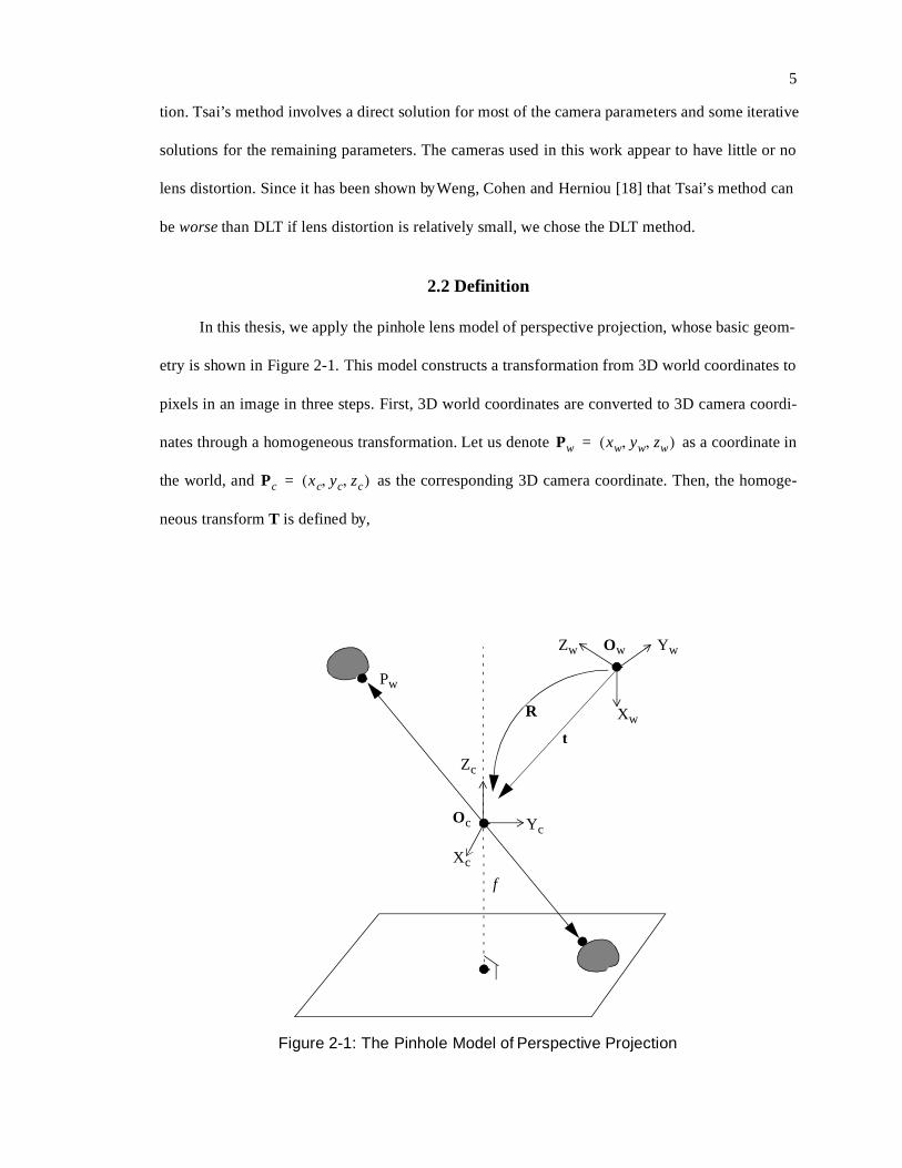
In this thesis, we apply the pinhole lens model of perspective projection, whose basic geom-

etry is shown in Figure 2-1. This model constructs a transformation from 3D world coordinates to

pixels in an image in three steps. First, 3D world coordinates are converted to 3D camera coordi-

nates through a homogeneous transformation. Let us denote as a coordinate in

the world, and as the corresponding 3D camera coordinate. Then, the homoge-

neous transform T is defined by,

Xw

YwZw Ow

Zc

Xc

YcOc

R

t

f

Figure 2-1: The Pinhole Model of Perspective Projection

Pw

Pw xw yw zw, ,( )=

Pc xc yc zc, ,( )=

6

(2-1)

such that,

(2-2)

where R denotes a rotation matrix,

(2-3)

and t denotes a translation vector,

. (2-4)

Second, the 3D camera coordinate is transformed to a 3D sensor coordinate :

(2-5)

where the camera’s intrinsic matrix K is defined as,

(2-6)

In equation (2-6) f is the effective focal length of the camera; a, b, and c describe the scaling

in x and y and the angle between the optical axis and the image sensor plane, respectively; and,

T R t000 1

≡

Pc

1T Pw

1=

3 3×

Rr11 r12 r13

r21 r22 r23

r31 r32 r33

≡

3 1×

ttx

ty

tz

≡

Pc Pu u v w, ,( )=

Pu

1K Pc

1=

K

fa– fb– uo– 0

0 fc– vo– 0

0 0 1 0

0 0 0 1

≡

uo

7

and are the offset from the image origin to the imaging sensor origin. Finally, the 3D sensor

coordinate is converted to the 2D image coordinate :

. (2-7)

The complete projection equation is therefore given by,

(2-8)

The transformation on the world coordinate in equation (2-8) can be combined into a

single matrix S. Since we are only interested in the overall transform between world coordinates

and image coordinates, and not an explicit solution of the extrinsic and/or intrinsic camera param-

eters, we therefore write,

(2-9)

or alternatively,

. (2-10)

2.3 Training the model

From equation (2-10), we now have a linear transformation with 12 unknowns that relate

world coordinates to image pixels. Each correspondence between a 3D world coordinate and a 2D

image point corresponds to a set of two equations,

vo

Pu xi yi,( )

xiuw----=

yivw----=

Pu

1KT Pw

1=

KT

Pu S Pw

1=

Pu

s11 s12 s13 s14

s21 s22 s23 s24

s31 s32 s33 s34

Pw

1=

8

(2-11)

or, in terms of the actual image coordinates,

(2-12)

Given a set of n pairs of world and image coordinates, equation (2-11) can be written in matrix

form as,

(2-13)

Arbitrarily setting leaves 11 unknown parameters which can be solved for using linear

regression. In general, the more correspondence pairs that are defined, the less susceptible the

model is to noise. To a large extent, this thesis aims to reduce or eliminate the need to collect many

such precise correspondence pairs, as that can be labor intensive and/or prone to human operator

error.

u s31x s32y s33z s34+ + +( ) w s11x s12y s13z s14+ + +( )=

v s31x s32y s33z s34+ + +( ) w s21x s22y s23z s24+ + +( )=

xi s31x s32y s33z s34+ + +( ) s11x s12y s13z s14+ + +( )=

yi s31x s32y s33z s34+ + +( ) s21x s22y s23z s24+ + +( )=

x y z 1 0 0 0 0 xix– xiy– xiz– xi–

0 0 0 0 x y z 1 yix– yiy– yiz– yi–

……

s11

s12

…s34

0=

s34 1=

CHAPTER 3 A SINGLE CAMERA

3.1 Introduction

A common method of calibration is to place a special object in the field of view of the cam-

era [10, 11, 16, 21]. Since the 3D shape of the object is known a priori, the 3D coordinates of spec-

ified reference points on the object can be defined in an object-relative coordinate system. One of

the more popular calibration objects described in the literature consists of a flat surface with a reg-

ular pattern marked on it. This pattern is typically chosen such that the image coordinates of the

projected reference points (corners, for example) can be measured with great accuracy. Given a

number of these points, each one yielding an equation of the form (2-9), the perspective transfor-

mation matrix S can be estimated with good results. One drawback of such techniques is that

sometimes a calibration object might not be available. Even when a calibration object is available,

the world coordinate system is defined by the placement of that object with respect to the camera,

and is not necessarily optimized to take advantage of the geometry of the scene.

In another popular method, called structure from motion, the camera is moved relative to the

world, and points of correspondence between consecutive images define the camera model [7, 21,

22]. In this approach, however, only the intrinsic parameters of the camera can be estimated (e.g.

the K matrix); as such, this method is used primarily for stereo vision and will be addressed in the

subsequent chapter.

In our work, we propose to divide the calibration process into two stages. First, we propose

to generate an initial “close” camera model, that then gets optimized to run-time quality through

standard machine learning techniques. Since our system will improve its model over time, all we

9

10

require initially is method for generating reasonably close calibrations without undue effort or

complexity. This type of problem was addressed by Worrall, et al. [19] through a graphical calibra-

tion tool, where the user can rotate and translate a known grid to the desired position on the image.

The system then calculates a perspective projection matrix S that will place the grid at that location

in the image. Our group has implemented a similar, intuitive GUI interface, which allows us to

generate fast and easy initial calibration estimates; this interface is described in further detail in

Appendix B.

3.2 Training Edges

Now, in order to improve the calibration model from the GUI interface through machine

learning, we need something for the machine learning algorithm to train on. Since we do not want

to require human operators to meticulously and precisely select numerous known correspondence

pairs in an image, we should select features in the image that can be easily isolated or extracted

through simple image processing techniques. In man-made environments, constrained edges with

known dimensions are frequent and stand out visually; some examples of these might be the inter-

section of the floor and a wall, the corner of a room, window sills, etc. These features can provide

a wealth of training data, without requiring explicit and precise image-to-world correspondence.

As such, we choose to rely on such constrained data for improving our initial camera calibration

model.

Exploiting the geometry of a given scene, a set of lines is chosen in 3D space, where each of

the lines is constrained along two dimensions; for example the vertical intersection of two perpen-

dicular walls is constrained by and where and are known constants. The

pixels corresponding to each of the lines and the constraints that define each line are the basis for

our model improvement algorithm. In order not to bias the training algorithm, the lines (edges)

x C0= y C1= C0 C1

11

should be chosen so as to provide training data that is balanced throughout the region of interest

both in area and scale as shown, for example, in Figure 3-1.

3.3 Optimization Criterion

Given our constrained-edges training data, we must define a reasonably well-behaved opti-

mization criterion that lets us know how the training algorithm is progressing. Care should be used

when choosing the optimization criterion, as it is the only mechanism a system has to evaluate a

potential model. After some experimentation, our final optimization criterion was designed to

reflect the error between the actual and projected pixel locations of the constrained edges and is

defined by,

(3-1)

where e denotes a training edge, i denotes a pixel along that edge, n denotes the number of pixels

along a particular edge, and m denotes the total number of edges. In equation (3-1), is defined

by,

(a) (b)

Figure 3-1: Example Training Edges

E 1m----

Eei

n-------

i 0=

n

∑e 0=

m

∑=

Eei

12

(3-2)

where is a actual pixel location in the training set and is the projected pixel loca-

tion, which is computed as follows. First, given the two constraints of a single edge (e.g. ,

), a pixel from the corresponding image line and the current perspective projection

model S, apply equation (2-11) to generate two equations and one unknown. For example, for the

constraints specified above, the two equations would become,

(3-3)

Equations (3-3) are easily generalized to arbitrary lines in space, and can be solved for the

unknown coordinate (or parameter, in the general case) through linear regression. Then, we can

project the resulting 3D coordinate onto the image, using equations (2-8) and (2-7), to get

The camera pespective will have some effect on the training data. Given two equal length

edges, the one with a larger image crossection will have more sample points and therefore will

contribute more to the error. To compensate for this, the error generated by each edge is averaged

to an error per pixel along that edge. The average error of each edge is then averaged to obtain the

final error measure E.

3.4 Initial Models

Error in a calibration model can be decomposed into three basic types: rotation, translation,

and scale. Any training algorithm may handle these different sources of error with varying degrees

of success. Therefore, we investigate how well our algorithm (defined below) performs on improv-

ing initial models in four general classes, as defined and illustrated in Figure 3-2. Each of the first

Eei 2 xs xp–( )2ys yp–( )2

+=

xs ys,( ) xp yp,( )

x C0=

y C1= xs ys,( )

s31xs s11–( )C0 s32xs s12–( )C1 s33xs s13–( )z+ + s14 s34xs–=

s31ys s21–( )C0 s32ys s22–( )C1 s33ys s23–( )z+ + s24 s34ys–=

xp yp,( )

13

three initial models in Figure 3-2 is labeled by the dominant type of error displayed. The fourth

model exhibits a combination of errors, but was generated to be fairly close to an acceptable final

model. Given a graphical calibration tool, as described in Appendix B, the close model represents

an easily achievable and therefore most likely starting configuration. The other three cases are pre-

sented to establish the limits of our training approach and to determine the types of error that

present the most difficulty.

3.5 Gradient Descent

The error measure defined in equation (3-2) can be expanded to,

(a) Close

(c) Scale

(b) Rotation

(d) Translation

Figure 3-2: Error Types of Initial Models

14

(3-4)

This is a differentiable function in S for which we can compute the gradient with respect to

the parameters in S such that,

. (3-5)

Note that since is assigned to be equal to one, it is not part of the gradient in equation (3-5).

From equation (3-1), the overall gradient is then given by,

. (3-6)

Given this gradient, the current model S can now be modified by a small positive constant in

the direction of the negative gradient,

. (3-7)

For error surfaces that can be roughly approximated as quadratic, we would expect the

model recursion in equation (3-7) to converge to a good near-optimal solution. Figure 3-3 below

illustrates the performance of pure gradient descent for the four types of initial models. From these

plots, it is apparent that the gradient descent recursion very quickly gets stuck in a local minimum

that is far from optimal; all four types of initial models caused gradient descent to fail within 2.75

seconds.1 In other words, the error surface is decidedly non-quadratic in a global sense, and gradi-

ent-descent represents at best only a partial training algorithm for this problem.

1. All experiments in this thesis were run on a 700 MHz Pentium III running Linux.

Eei 2 xs

s11x s12y s13z s14+ + +

s31x s32y s33z s34+ + +---------------------------------------------------------–

2ys

s21x s22y s23z s24+ + +

s31x s32y s33z s34+ + +-------------------------------------------------------–

2+=

E∇ ei

E∇ eis11∂

∂Eei …s33∂

∂Eei

T

=

s34

E∇

E∇ 1m----

E∇ ei

n------------

i 0=

n

∑e 0=

m

∑=

δg

Snew 1 Eδg∇–( )S=

15

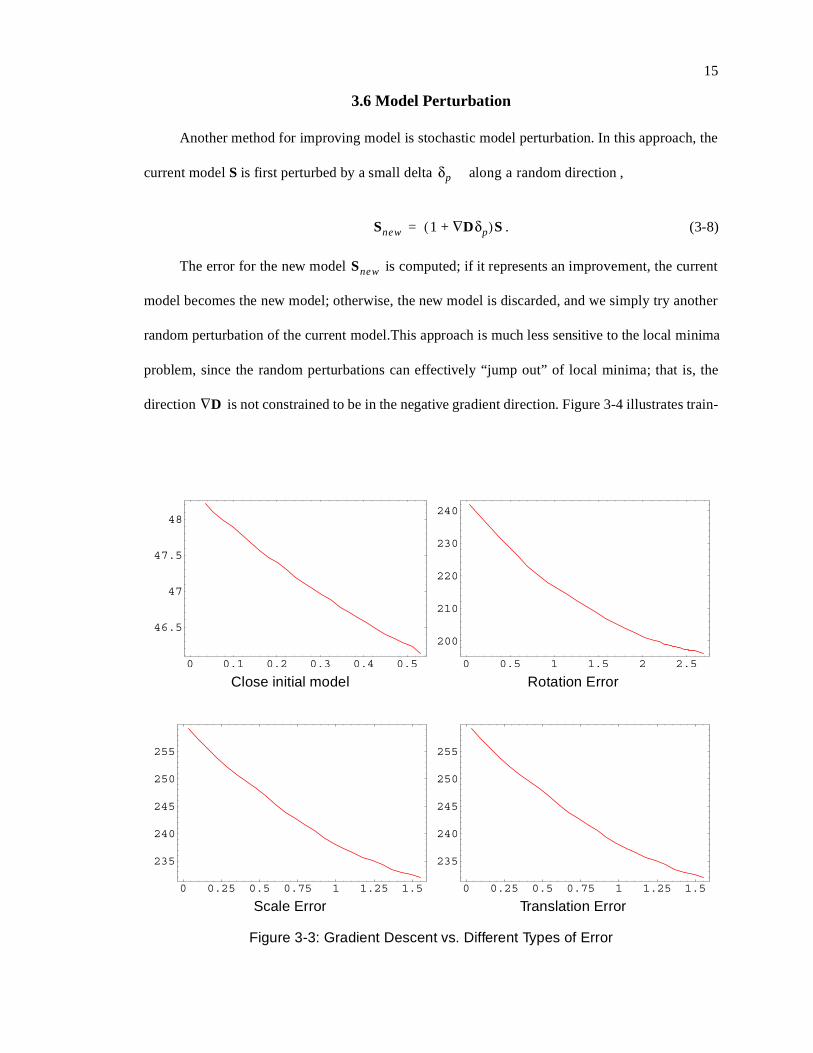
3.6 Model Perturbation

Another method for improving model is stochastic model perturbation. In this approach, the

current model S is first perturbed by a small delta along a random direction ,

. (3-8)

The error for the new model is computed; if it represents an improvement, the current

model becomes the new model; otherwise, the new model is discarded, and we simply try another

random perturbation of the current model.This approach is much less sensitive to the local minima

problem, since the random perturbations can effectively “jump out” of local minima; that is, the

direction is not constrained to be in the negative gradient direction. Figure 3-4 illustrates train-

0 0.5 1 1.5 2 2.5

200

210

220

230

240

0 0.25 0.5 0.75 1 1.25 1.5

235

240

245

250

255

0 0.25 0.5 0.75 1 1.25 1.5

235

240

245

250

255

0 0.1 0.2 0.3 0.4 0.5

46.5

47

47.5

48

Close initial model Rotation Error

Scale Error Translation Error

Figure 3-3: Gradient Descent vs. Different Types of Error

δp

Snew 1 Dδp∇+( )S=

Snew

D∇

16

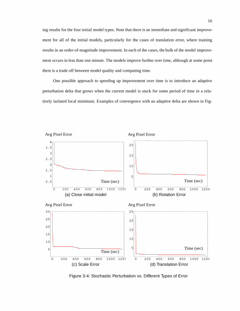
ing results for the four initial model types. Note that there is an immediate and significant improve-

ment for all of the initial models, particularly for the cases of translation error, where training

results in an order-of-magnitude improvement. In each of the cases, the bulk of the model improve-

ment occurs in less than one minute. The models improve further over time, although at some point

there is a trade off between model quality and computing time.

One possible approach to speeding up improvement over time is to introduce an adaptive

perturbation delta that grows when the current model is stuck for some period of time in a rela-

tively isolated local minimum. Examples of convergence with an adaptive delta are shown in Fig-

0 200 400 600 800 1000 1200

5

10

15

20

0 200 400 600 800 1000 1200

5

10

15

20

25

30

0 200 400 600 800 1000 1200

5

10

15

20

25

0 200 400 600 800 1000 1200

0.5

1

1.5

2

2.5

3

3.5

4

(a) Close initial model (b) Rotation Error

(c) Scale Error (d) Translation Error

Figure 3-4: Stochastic Perturbation vs. Different Types of Error

Avg Pixel Error Avg Pixel Error

Avg Pixel Error Avg Pixel Error

Time (sec)

Time (sec) Time (sec)

Time (sec)

17

ure 3-5. Not surprisingly, the results are very similar, but the adaptive delta does improve

performance slightly, and, we expect, would increasingly improve performance if used over a

longer period on time.

0 200 400 600 800 1000 1200

5

10

15

20

0 200 400 600 800 1000 1200

5

10

15

20

25

30

0 200 400 600 800 1000 1200

5

10

15

20

25

0 200 400 600 800 1000 1200

0.5

1

1.5

2

2.5

3

3.5

4



Figure 3-5: Stochastic Perturbation with Adaptive Delta vs. Different Types of Error

Time (sec)

Avg Pixel Error

Avg Pixel Error

Avg Pixel Error

Avg Pixel Error


Time (sec)

18

3.7 Gradient-Peturbation Hybrid

Given the relative speed of convergence of gradient descent in localized near quadratic

neighborhoods, and the insensitivity of stochastic perturbation to local minima, a combination of

gradient descent and model perturbation may well train faster than either approach by itself. In this

hybrid approach, gradient descent will quickly reach local minima, at which point, adaptive-delta

model perturbation takes over to search for better regions in model parameter space. In other

words, gradient descent and stochastic perturbation alternate in optimizing the camera model over

time. Sample results for this approach are shown in Figure 3-6.

0 200 400 600 800 1000 1200

5

10

15

20

0 200 400 600 800 1000 1200

5

10

15

20

25

30

0 200 400 600 800 1000

5

10

15

20

25

0 200 400 600 800 1000

1

2

3

4



Figure 3-6: Gradient-Perturbation Hybrid vs. Different Types of Error

Avg Pixel Error

Time (sec)

Avg Pixel Error

Time (sec)

Time (sec)

Avg Pixel ErrorAvg Pixel Error

Time (sec)

19

3.8 Performance Comparisons

Which approach is best for our purposes depends on a number of different criteria. Ideally,

we would like a method that responds quickly, improves in the face of difficult models, and is able

to continue to improve if given an open-ended amount of time. As we have already seen, and as we

further detail in Tables 3-1, 3-2 and 3-3, each method improves the camera model the most within

Table 3-1: Model Perturbation: Average Error Per Pixel

Initial 20 Sec. 1 Min. 5 Min. 10 Min. 20 Min.

Close 3.9336 2.0053 1.9618 1.6327 1.5182 1.4246

Rotation 21.2163 8.8545 6.5318 6.2082 6.1391 5.8464

Scale 28.9091 6.9955 6.9518 6.8318 5.4664 5.2064

Translation 23.0482 1.7082 1.6143 1.3182 1.1909 1.1618

Table 3-2: Model Perturbation With Adaptive Delta: Average Error Per Pixel


Close 3.9336 2.0053 1.9691 1.64 1.5972 1.4127

Rotation 21.2163 9.138 6.8472 6.22 5.9091 5.2491

Scale 28.9091 7.0035 6.9515 5.8091 5.2945 4.5236

Translation 23.0482 1.7082 1.6145 1.3255 1.2227 1.19

Table 3-3: Gradient - Perturbation Hybrid: Average Error Per Pixel


Close 3.9336 2.0364 1.9173 1.5664 1.4736 1.3355

Rotation 21.2164 12.4909 8.0218 5.3855 5.1991 5.0564

Scale 28.9091 14.13 6.7918 5.7545 5.5655 4.6891

Translation 23.0482 1.6909 1.5627 1.4 1.3118 1.1964

20

the first minute of training. For each approach the error then continues to decline, but the two tech-

niques that make use of an adaptive delta show a continuing ability to improve over time with the

hybrid approach outperforming the others. A direct comparison is shown in Figures 3-7 and 3-8,

0 200 400 600 800 1000

-0.04

-0.02

0

0.02

0 200 400 600 800 1000

-0.2

-0.1

0

0.1

0 200 400 600 800 1000-0.2

-0.15

-0.1

-0.05

0

0.05

0.1

0 200 400 600 800 1000-0.5

-0.25

0

0.25

0.5

0.75

1

0 200 400 600 800 1000

-1

-0.5

0

0.5

1

0 200 400 600 800 1000

-1.5

-1

-0.5

0

0.5

Translation Scale

Perturbation - Perturbation with delta Perturbation - Perturbation with delta

Perturbation - Hybrid Perturbation - Hybrid

Perturbation with Delta - HybridPerturbation with Delta - Hybrid

Figure 3-7: Performance Comparison for the Translational and Scale Initial Models

Time (sec)

Pixels

Pixels

Pixels Pixels

Time (sec)Time (sec)

Pixels


Pixels

Time (sec)

21

which plot the difference in error between the different techniques over time. The final camera

models trained by the hybrid method are depicted in Figure 3-9.

0 200 400 600 800 1000

-0.08

-0.06

-0.04

-0.02

0

0.02

0 200 400 600 800 1000

-0.02

0

0.02

0.04

0.06

0.08

0 200 400 600 800 1000

-0.025

0

0.025

0.05

0.075

0.1

0.125

0 200 400 600 800 1000-0.6

-0.4

-0.2

0

0.2

0.4

0 200 400 600 800 1000

0

0.2

0.4

0.6

0.8

0 200 400 600 800 1000

-0.5

-0.25

0

0.25

0.5

0.75

Close Rotation

Perturbation - Perturbation with delta Perturbation - Perturbation with delta

Perturbation - Hybrid Perturbation - Hybrid

Perturbation with Delta - HybridPerturbation with Delta - Hybrid

Figure 3-8: Performance Comparison for the Close and Rotational Initial Models

Pixels

Time (sec)

Pixels


Pixels

PixelsPixels

Time (sec)


Pixels

22

Why does training virtually eliminate translation error while rotation and scale errors prove

more difficult to correct? The answer lies in the camera model itself [see equation (2-8)]. Transla-

tion is parameterized by 3 of the 12 parameters in S, while rotation is parameterized by 9 parame-

ters, which are additionally constrained by the orthonormality requirement for rotation matrices.

Finally, scale affects all 12 parameters in S. Thus, to correct rotational errors, 9 model parameters

must be changed simultaneously, while for scale errors, all 12 parameters must be changed. This

adds complexity and size to the search space, resulting in a slower improvement and a greater like-

lihood of getting stuck in a remote local minimum.

(a) Close

(c) Scale

(b) Rotation

(d) Translation

Figure 3-9: Final Models Using the Gradient - Perturbation Hybrid Technique

CHAPTER 4STEREO CAMERAS

4.1 Introduction

We are interested in abstracting 3D information about the world through computer vision

techniques. Therefore, we will, in general, require more than one non-coincident camera view for

an area of interest, since pixels from a single-camera image do not correspond to exact 3D world

coordinates, but rather to rays in space. If we can establish a feature correspondence between at

least two camera views calibrated to the same world coordinate system, then we can extract the

underlying 3D information for that feature by intersecting the rays corresponding to its pixel loca-

tion in each image. Hence, in this chapter, we consider the problem of simultaneous calibration of

multiple (stereo) fixed cameras to a unique world coordinate system. More specifically, we build

on the results of the previous chapter by assuming that one camera in a multi-camera setup has

already been trained towards a good model. The task that remains is to calibrate the additional

camera(s). In the remainder of this chapter, we focus on the two-camera case, although our results

generalize in a straightforward manner to more than two cameras.

Given a set of two cameras where one has already been trained, and the second has a rough

initial calibration, we propose to improve the second calibration through an iterative process that

involves using a “virtual calibration object.” This calibration object is created by moving a physical

object throughout the area of interest and tracking it from each camera view. The path that the

object follows in the image (in pixels) and the corresponding 3D estimates constitute the training

data at each step of the algorithm.

23

24

4.2 Related Work

Previous work in stereo camera calibration is relatively extensive, but varies based on the

particular application of interest. Many of the previous methods use a known calibration pattern

whose features are extracted from each image. Rander and Kanade [12] have a system of approxi-

mately 50 cameras arranged in a dome to observe a room-sized space. In order to calibrate these

cameras, a large calibration object is built and then moved to several precise locations, in effect

building a virtual calibration object that covers most of the room. Do [4] applied a neural network

to acquire stereo calibration models and determined the approach to be adequate; however, he went

on to show that high accuracy did not appear possible in a reasonable amount of training time.

Horaud et al. [7] use rigid and constrained motions of a stereo rig to allow camera calibration. This

approach, like most in the field, address small baseline-stereo rigs which usually have a fixed, rigid

geometry. Azarbayejani and Pentland [2] propose an approach that tracks an item of interest

through images to obtain useable training data. This approach is similar to ours except that they

use object tracking to completely establish a calibration rather than using it to modify an already

existing calibration. The drawback of this technique is that scale is not recoverable, so absolute

distance has no meaning. Chen et al. [3] offer a similar technique that uses structure-from-motion

to obtain initial camera calibration models, and then tracks a virtual calibration object to iterate to

better models. The initial calibrations are obtained sequentially, where each new calibration model

depends on those previously derived. As such, error accumulates for each sucessive calibration,

placing newer calibrations further away from an optimal solution. Our work has shown (e.g. Fig-

ures 3-4, 3-5 and 3-6) that this can have a significant impact on both the final calibration obtained

and the amount of time required to obtain it.

25

4.3 Our Approach

In this research, our primary motivation is to make the calibration process as quick and easy

as possible without sacrificing precision. We wish for a non-expert to be able to completely cali-

brate a system for operation by making part of the calibration process visual and automating the

rest. Each camera obtains its initial calibration via a graphical calibration tool (as described in

Appendix B). The calibration is then improved by having the cameras track an object of interest

throughout the viewing area. Ideally, image capture and processing should be synchronized

between cameras; however, in practice, such synchronization is difficult and expensive to achieve

in hardware. Even for an asynchronous system, however, we can approximate synchronous opera-

tion through Kalman filtering and interpolation of time-stamped images, as long as the system

clocks are synchronized between the image processing computers. This Kalman-filtered and inter-

polated trajectory then becomes the training data for improving our stereo camera models.

4.4 Training Data

In order to collect training data, we apply a modified version of Zapata’s color-model-based

tracking algorithm [20] to track an object of interest from multiple camera views in real-time. The

time-stamped pixel data of the object’s centroid are passed through a first-order Kalman filter and

then sent to a multi-camera data fusor. The data fusor accepts the time-stamped data streams, inter-

polating and synchronizing the multiple data streams at 30Hz. Prior to training, the synchronized

tracking data is balanced so that no one single region of the image is dominated by a disproportion-

ately large amount of data. Although training examples reported in this thesis are over fixed data

sets, there is no algorithmic obstacle to training off streaming data in real-time.

4.5 Model Improvement

The training data now consists of synchronized sets of pixel values from the multiple

cameras. Let us consider the set of pixel values for the object at time :

n m

t

26

(4-1)

where denotes the pixel location of the object for camera . Given our current estimate of

each camera model , we can estimate the 3D world coordinate of the object at time by regress-

ing the equations,

(4-2)

, for , which denotes the estimated 3D world coordinate at time .

For each training camera, we now have estimated correspondence pairs between the syn-

chronized pixel values for that camera and their corresponding estimated 3D world coordinates.

Given this data, we can now apply equation (2-13) to generate a new perspective projection matrix

based on the estimated 3D tracking data. This process is repeated until the calibration

reaches acceptable precision. Figure 4-1 shows the error over time for the above approach. There is

initial improvement followed by rapid and consistent model degradation. This is not what was

expected, but can be explained after looking a little closer at the procedure and how it operates.

The resulting calibration in Figure 4-1 gives an indication of the source of the problem. Recall

from equation (2-8) that part of the projection matrix is the camera matrix K which contains intri-

nisic parameters for the camera such as scale, skew and offset. These parameters are fixed in real-

ity but are obviously being changed by this training process. This is happening due to the

unconstrained nature of the training process: known incorrect (x, y, z) are being used to train a

model which is simply a linear least squares solution and K, as a component of this model, is also

being changed. We are seeking to use a good model to train a bad model by modifing its rotation

and translation, not its intrinsic camera parameters. A property of the linear least squares estimate

x1 y1,( ) x2 y2,( ) … xm ym,( ), , ,{ }t

xj yj,( ) j

Sj t

s31 j, xj s11 j,–( )xt s32 j, xj s12 j,–( )yt s33 j, xj s13 j,–( )zt+ + s14 j, s34 j, xj–=

s31 j, yj s21 j,–( )xt s32 j, yj s22 j,–( )yt s33 j, yj s23 j,–( )zt+ + s24 j, s34 j, yj–=

j 1 2 … m, , ,{ }∈ xt yt zt, ,( ) t

n

Sj new,

27

is that it distributes the error as evenly as possible between the two models. The even distribution

of the error is not appropriate for us since we know that the source of the error is the bad model.

Weighing the parameters of the regression towards the training model as an indication that it is the

source of the error might help. Figure 4-2 shows the error vs. time as a function of different

weights applied to the training model. It shows that we can mitigate the effect on the K matrix of

the training model with a weighted regression. A gain of ten shows better performance but is still

unstable. A gain of 100 or 1000 shows much better stability and performance. Looking at the error

over time for the different gains it appears that a higher gain exibits a similar response when

viewed on a larger scale.

0 25 50 75 100 125 150 1750

200

400

600

800

(b) Initial Calibration(a) Error Over Time

(d) Final Calibration(c) Best Calibration

Figure 4-1: Results for a Non-Weighted Model Improvement

Error (mm)

Time (sec)

28

0 25 50 75 100 125 150 175

10

20

30

40

50

60

70

80

0 25 50 75 100 125 150 175

10

20

30

40

50

60

70

80

0 25 50 75 100 125 150 175

10

20

30

40

50

60

70

80

0 200 400 600 800 1000 1200 1400

20

40

60

80

100

(a) Gain of 10 on Training Modell (b) Gain of 100 on Training Model

(c) Gain of 1000 on Training Model (d) Gain of 10000 on Training Model

Figure 4-2: Error Over Time for Various Gains on the Training Model

Time (sec)


Time (sec)

Error (mm)

Error (mm) Error (mm)

Error (mm)

29

0 25 50 75 100 125 150 1750

200

400

600

800

0 25 50 75 100 125 150 175

10

20

30

40

50

60

70

80

0 250 500 750 1000 1250 1500

20

40

60

80

100

0 100 200 300

20

40

60

80

100

(a) Gain of 1 (b) Gain of 10

(c) Gain of 100 (d) Gain of 1000

Figure 4-3: The Long Term Performance using Various Gains

Error (mm)

Time (sec)

Time (sec)

Error (mm)

Time (sec)

Error (mm)Error (mm)

Time (sec)

CHAPTER 5 FURTHER RESULTS AND DISCUSSION

5.1 Single Camera

Here, we present some further results for the algorithms developed in the previous two chap-

ters. Below, we solve eight sample calibration problems, where the initial calibrations are obtained

using our previously referenced graphical calibration tool These are shown in Figures 5-1, 5-2, 5-3

and 5-4. Given these descent initial calibrations, our algorithms develop run-time quality models

within two minutes from the start of training. Figures 5-5 and 5-6 show the systems perfor-

mance in the face of poor initial calibrations. These figures show that even a poor initial

calibration can be improved significantly, but not always to run-time quality. Overall, these

results show that our single-camera calibration approach meets our goal — namely, mak-

ing camera calibration a simpler, faster and easier process.

5.2 Stereo Cameras

Figure 5-7 and Figure 5-8 show four example calibrations obtained from two different cam-

era angles. The initial calibrations are obtained using our graphical calibration tool. These calibra-

tions and the associated graphs reveal the capabilities and shortcomings of our proposed stereo

technique. While in its present form, it may not yet be sufficiently robust for real world applica-

tion, it can certainly be made to be so with minor changes. As we discussed in Chapter 4, if we

constrained modifications of the camera model to extrinsic parameters only, keeping the intrinsic

parameters of the model fixed, we expect that the observed model drift would no longer occur.

30

31

0 20 40 60 80 100

1

2

3

4

5

6

0 500 1000 1500 2000

1

2

3

4

5

6

7

(a) Example 1 Initial

(c) Example 2 Initial

(b) Example 1 Final

(d) Example 2 Final

Figure 5-1: Example Single Camera Calibrations (1 & 2)

(f) Example 2 Error vs. Time(e) Example 1 Error vs. Time

32

0 500 1000 1500 2000

0.5

1

1.5

2

2.5

3

3.5

4

0 500 1000 1500 2000

1

2

3

4

5



(b) Example 3 Final

(d) Example 4 Final



33

0 500 1000 1500 2000

2.5

5

7.5

10

12.5

15

17.5

0 200 400 600 800 1000 1200 1400

1

2

3

4

5

6

7



(b) Example 5 Final

(d) Example 6 Final



34

0 200 400 600 800

1

2

3

4

5

6

7

0 100 200 300 400 500

2

4

6

8



(b) Example 7 Final

(d) Example 8 Final



35

0 50 100 150 200 250 300 350

2

4

6

8

10

12

14

16

0 100 200 300 400 500 600

5

10

15

20

(a) Poor Calibration 1 Initial

(c) Poor Calibration 2 Initial

(b) Poor Calibration 1 Final

(d) Poor Calibration 2 Final

Figure 5-5: Poor Initial Calibrations (1 & 2)

(f) Poor Calibration 2 Error vs. Time(e) Poor Calibration 1 Error vs. Time

36

0 100 200 300 400 500 600

2

4

6

8

10

12

14

16

0 100 200 300 400 500

5

10

15

20

25

(a) Poor Calibration 3 Initial

(c) Poor Calibration 4 Initial

(b) Poor Calibration 3 Final

(d) Poor Calibration 4 Final

Figure 5-6: Poor Initial Calibrations (3 & 4)

(f) Poor Calibration 4 Error vs. Time(e) Poor Calibration 3 Error vs. Time

37

0 20 40 60 80 100 120 140

30

40

50

60

70

80

0 50 100 150 200 250

50

60

70

80

90

(a) Initial Stereo Calibration 1

(c) Initial Stereo Calibration 2

(b) Final Stereo Calibration 1

(d) Final Stereo Calibration 2

Figure 5-7: Stereo Calibration Examples (1 & 2)

(f) Calibration 2 Error vs. Time(e) Calibration 1 Error vs. Time

38

0 50 100 150 200

42.5

45

47.5

50

52.5

55

57.5

60

0 25 50 75 100 125 150 175

30

40

50

60

70

80

90

100

(a) Initial Stereo Calibration 3

(c) Initial Stereo Calibration 4

(b) Final Stereo Calibration 3

(d) Final Stereo Calibration 4

Figure 5-8: Stereo Calibration Examples (3 & 4)

(f) Calibration 4 Error vs. Time(e) Calibration 3 Error vs. Time

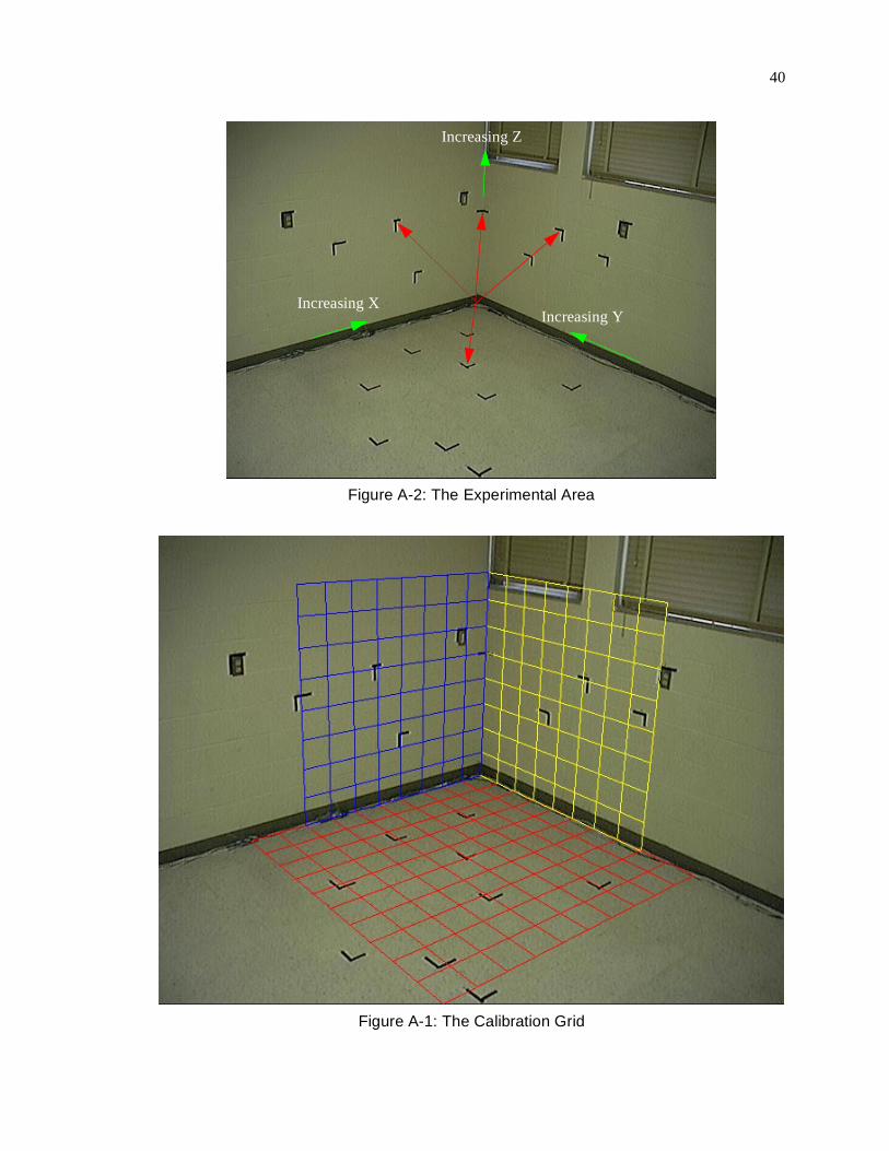
APPENDIX AVISUAL CALIBRATION EVALUATION

When applying machine learning to improve camera models, an well-behaved error measure

is critical. With exact correspondence data (2D image coordinates paired with 3D world coordi-

nates), such an error measure is easily specified. It is precisely this type of data that we want to

avoid having to collect, however. Yet, without such data, it is difficult, if not impossible, to define a

globally well-behaved error measure. As such, we choose the human eye as an appropriate means

of evaluating different calibration models. To make this intuitive, we draw a grid defined in space

onto the image using the current camera model, and decide visually if the system’s error measure

is accurately measuring the quality of a model. This grid is chosen to match some feature(s) in the

scene to allow a person to visually determine the quality of a calibration. Figure A-2 shows the

experimental area. In Figure A-2, the red arrows indicate the corner points of a one meter cube

placed in the far corner of the room, while the green arrows show the world coordinate system,

defined after considering the experimental area and how to keep initial data collection as simple as

possible. Figure A-1 shows a sample grid drawn on an image. The grid uses squares and

should ideally be aligned with the floor and walls. Points marked with a red arrow in Figure A-2

should have the outside corner of the fifth box out or up laying on it. The windowsill is a straight

edge that a human can use as a guide for the top edge of the grid.

20cm2

39

40

Figure A-1: The Calibration Grid

Increasing XIncreasing Y

Increasing Z

Figure A-2: The Experimental Area

APPENDIX BGRAPHICAL CALIBRATION TOOL

In order to generate initial rough calibration models quickly and easily, we developed an

intuitive graphical interface through which a user can manipulate and align a grid model of a scene

for different rotations and translations of the camera with respect to the world. This interface, as

shown in Figure B-1, was written in C for the X/Motif window system.

Given approximate intrinsic parameters for a camera, we can project a three-dimensional

model of the world onto an image for any given rotation, translation and scale (effective focal

length). Therefore, as the user adjusts parameters that control scale, rotation and translation, the

grid model of the world is continuously redrawn to reflect the new effective pose of the camera.

Once the user is happy with the alignment of the grid model to the world, he/she can then save the

effective perspective projection matrix and use that as the initial camera calibration model.

41

42

Figure B-1: The Graphical Calibration Tool

REFERENCES

[1] Y. I. Abdel-Aziz and H. M. Kahara, “Direct Linear Transformation From Comparator Coor-dinates into Object-Space Coordinates,” Proc. American Society of Photogrammetry Sympo-sium on Close Range Photogrammetry, pp. 1-18, 1971.

[2] A. Azarbayejani and A. Pentland, “Camera Self Calibration From One Point Correspon-dence,” Perceptual Computing Technical Report #341, Massachusetts Institute of Technol-ogy Media Library, 1995.

[3] X. Chen, J. Davis and P. Slusallek, “Wide Area Calibration Using Virtual CalibrationObjects,” Proc. IEEE Conf. on Computer Vision and Pattern Recognition, vol. 2, pp. 520-7,2000.

[4] Y. Do, “Application of Neural Networks for Stereo-Camera Calibration,” Proc. Int. JointConf. on Neural Networks, vol. 4, pp 2719-22, 1999.

[5] R. Frezza and C. Altafini, “Autonomous Landing by Computer Vision: An Application ofPath following in SE(3),” Proc. IEEE Conf. on Decision and Control, vol. 3, pp. 2527-32,2000.

[6] I. Haritaoglu, D. Harwood and L. Davis, “ : Who? When? Where? What? A Real TimeSystem for Detecting and Tracking People,” Proc. IEEE Int. Conf. on Face and Gesture Rec-ognition, pp. 222-7, 1998.

[7] R. Horaud, G. Csurka and D. Demirdijian, “Stereo Calibration from Rigid Motions,” IEEETrans. on Pattern and Machine Intelligence, vol. 22, no. 12, pp. 1446-52, 2000.

[8] S. Kamijo, Y. Matsushita, K. Ikeuchi and M. Sakauchi, “Traffic Monitoring and AccidentDetection at Intersections,” IEEE Trans. on Intelligent Transportation Systems, vol. 1, no. 2,pp. 108-18, 2000.

[9] F. Karbou and F. Karbou, “An Interval Approach to Handwriting Recognition,” Proc. Conf.of the North American Fuzzy Information Processing Society, pp. 153-7, 2000.

[10] J.M. Lee, B.H. Kim, M.H. Lee, K. Son, M.C. Lee, J.W. Choi and S.H. Han, “Fine Active Cal-ibration of Camera Position/Orientation Through Pattern Recognition,” IEEE Int. Symposiumon Industrial Electronics, vol. 2, pp. 657-62, 1998.

[11] P. Mendonca and R. Cipolla, “A Simple Technique for Self-Calibration,” Proc. IEEE Conf. onComputer Vision and Pattern Recognition, vol. 1, pp. 500-5, 1999.

W4

43

44

[12] P. Rander, “A Multi-Camera Method for 3D Digitization of Dynamic, Real-World Events,”CMU-RI-TR-98-12, Technical Report, The Robotics Institute, Carnegie Mellon University,1998.

[13] G. Rigoll, S. Eickeler and S. Muller, “Person Tracking in Real-World Scenarios Using Statis-tical Methods,” Proc. IEEE Int. Conf. on Automatic Face and Gesture Recognition, pp.342-7,2000.

[14] H. Schneiderman, “A Statistical Approach to 3D Object Detection Applied to Faces andCars,” CMU-RI-TR-00-06, Ph.D. Thesis, The Robotics Institute, Carnegie Mellon Univer-sity, 2000.

[15] R. Sharma, M. Zeller, V.I. Pavlovic, T.S. Huang, Z. Lo, S. Chu, Y. Zhao, J.C. Phillips and K.Schulten. “Speech/Gesture Interface to a Visual-Computing Environment,” IEEE ComputerGraphics and Applications, vol. 20, no. 2, pp. 29-37, 2000.

[16] R. Tsai, “A Versatile Camera Calibration Technique for High-Accuracy 3D Machine VisionMetrology Using Off-the-Shelf TV Cameras and Lenses,” IEEE Journal of Robotics andAutomation, vol. RA-3, no. 4, pp 323-44, 1987.

[17] H. Wang, W. Hsu, K. Guan and M. Lee, “An Effective Approach to Detect Lesions in ColorRetinal Images,” Proc. IEEE Conf. on Computer Vision an Pattern Recognition, vol. 2, pp.181-6, 2000.

[18] J. Weng, P. Cohen and M. Herniou, “Camera Calibration with Distortion Models and Accu-racy Evaluation,” IEEE Trans. of Pattern Analysis and Machine Intelligence, vol. 14, no. 10,pp. 965-80, 1992.

[19] A.D.Worrall, G.D.Sullivan and K.D.Baker, “A Simple Intuitive Camera Calibration Tool ForNatural Images,” Proc. of the 5th British Machine Vision Conf., vol. 2, pp. 781-90, 1994.

[20] I. Zapata, “Detecting Humans in Video Sequences Using Color and Shape Information,” M.S.Thesis, Dept. of Electrical and Computer Engineering, University of Florida, 2001.

[21] Z. Zhang, “A Flexible Technique for Camera Calibration,” IEEE Trans. on Pattern Analysisand Machine Intelligence, vol.22, no.11, pp. 1330-4, 2000.

[22] Z. Zhang, “Motion and Structure of Four Points from One Motion of a Stereo Rig withUnknown Extrinsic Parameters,” IEEE Trans. on Pattern Analysis and Machine Intelligence,vol. 17, no. 12, pp. 1222-5, 1995.

45

BIOGRAPHICAL SKETCH

Scott Nichols was born in Miami, Florida, in 1969. A high school dropout, Scott decided to

pursue an education and started community college full-time in 1994. He transferred as a junior to

the University of Florida in 1996 and recieved both a Bachelor of Science degree in electrical engi-

neering and a Bachelor of Science degree in computer engineering in Aug 1999. He has since

worked as a research assistant at the Machine Intelligence Laboratory, working toward a Master of

Science degree in electrical engineering.

Improvement of the Camera Calibration through the...

Documents

Transcript of Improvement of the Camera Calibration through the...