
Improved Transport Terminal Utilization: The Case Of ...
14
Improved Transport Terminal Utilization: The Case Of Jordan Wharf, Guimaras Raymund Paolo B. ABAD Graduate Student Civil Engineering Department De La Salle University 2401 Taft Avenue, Manila, 1004 E-mail: [email protected] Alexis M. FILLONE Associate Professor Civil Engineering Department De La Salle University 2401 Taft Avenue, Manila, 1004 E-mail: [email protected] Abstract: Public transport in the Philippines comes in different modes depending on the geography. For Guimaras island province, commuters depend on both land and water transport to carry out their daily trip activities. Despite the high number of public transport services, transport operators do not practice methods on improving its service reliability. This paper focused on improving the efficiency of operations of land and water transport by reducing the number of waiting vehicles at the wharf. The reduction was done by determining the design frequency to accommodate the passenger volume using the percentages of modal shares. A proposed fleet size was given to further improve the efficiency of the wharf operations. The service operating characteristics of the wharf and of the public transports were determined by a detailed survey plan. The results show a significant decrease in number of waiting vehicles at the wharf and an increase in utilization coefficients. Key Words: Public transport, Water transport, Public transport demand and supply 1. INTRODUCTION Public transportation plays a vital role in promoting the mobility of individuals to their respective destinations. It is for this reason that there has been a thrust in improving the service reliability of public transportation. From the perspective of the passengers, the reliability attributes that are of concern are: waiting time, boarding time, in-vehicle time, alighting time, total travel time, transfer time, pre-trip information time, pre-trip time required for changes in access path, and seat availability (Ceder, 2007). Intermodal transportation has been defined by Jones et al. (2000) as the shipment of cargo and the movement of people that makes use of more than one mode of transport during a single journey. Intermodality aims to optimize the traveling conditions considering the advantages and disadvantages of each mode of transport. The transferring from one mode of transport to another mode has been considered as the “weak” link. It is for this reason that efficient operations of intermodal stations are of utmost importance. In order to attain such the terminal should provide: (1) a reliable and adequate level of service in the operation of the terminal; (2) satisfactory facilities serving the transfer; (3) provision of low cost travel; (4) sufficient accessibility to the terminal across all users; (5) reduction in travel time compared to the travel time without transfer; and (6) direct access between platforms of different modes serving the (Pitsiava-Latinopoulou & Iordanopoulus, 2012). The number of modes and vehicles types, the operating time period with its desirable level
Transcript of Improved Transport Terminal Utilization: The Case Of ...

�����������������������
����� ��������������������������������������������������������������������������
������������������������� � ������
Improved Transport Terminal Utilization:
The Case Of Jordan Wharf, Guimaras
Raymund Paolo B. ABAD Graduate Student Civil Engineering Department De La Salle University 2401 Taft Avenue, Manila, 1004 E-mail: [email protected]
Alexis M. FILLONE Associate Professor Civil Engineering Department De La Salle University 2401 Taft Avenue, Manila, 1004 E-mail: [email protected]
Abstract: Public transport in the Philippines comes in different modes depending on the geography. For Guimaras island province, commuters depend on both land and water transport to carry out their daily trip activities. Despite the high number of public transport services, transport operators do not practice methods on improving its service reliability. This paper focused on improving the efficiency of operations of land and water transport by reducing the number of waiting vehicles at the wharf. The reduction was done by determining the design frequency to accommodate the passenger volume using the percentages of modal shares. A proposed fleet size was given to further improve the efficiency of the wharf operations. The service operating characteristics of the wharf and of the public transports were determined by a detailed survey plan. The results show a significant decrease in number of waiting vehicles at the wharf and an increase in utilization coefficients. Key Words: Public transport, Water transport, Public transport demand and supply 1. INTRODUCTION Public transportation plays a vital role in promoting the mobility of individuals to their respective destinations. It is for this reason that there has been a thrust in improving the service reliability of public transportation. From the perspective of the passengers, the reliability attributes that are of concern are: waiting time, boarding time, in-vehicle time, alighting time, total travel time, transfer time, pre-trip information time, pre-trip time required for changes in access path, and seat availability (Ceder, 2007). Intermodal transportation has been defined by Jones et al. (2000) as the shipment of cargo and the movement of people that makes use of more than one mode of transport during a single journey. Intermodality aims to optimize the traveling conditions considering the advantages and disadvantages of each mode of transport. The transferring from one mode of transport to another mode has been considered as the “weak” link. It is for this reason that efficient operations of intermodal stations are of utmost importance. In order to attain such the terminal should provide: (1) a reliable and adequate level of service in the operation of the terminal; (2) satisfactory facilities serving the transfer; (3) provision of low cost travel; (4) sufficient accessibility to the terminal across all users; (5) reduction in travel time compared to the travel time without transfer; and (6) direct access between platforms of different modes serving the (Pitsiava-Latinopoulou & Iordanopoulus, 2012). The number of modes and vehicles types, the operating time period with its desirable level

�����������������������
����� ��������������������������������������������������������������������������
������������������������� � ������
of service, the expected level of activity in terms of passenger volume, frequencies, and waiting times, and the seasonal variations in demand are some elements that should be identified in the design or redesign of a terminal (Rivasplata, 2011). In cases that these are not taken into consideration, there would be negative impacts that would affect the efficiency of operations, safety of passengers, and travel reliability. Positive impacts as presented by Henry et al. (2008) include decrease in transportation costs, increase economic productivity and efficiency, reduce the stresses induced on the infrastructure components, and reduce in energy consumption. This study would focus on the reduction of the number of operating vehicles in an intermodal transportation terminal in Western Visayas, Philippines. In the country, there are different modes of transport and there are only a few studies that focus on vehicle scheduling. The study of Kang et al. (2010) provided a heuristic procedure to determine the optimal frequency of jeepney operations in Metro Manila based on maximum load, load factor, and vehicle capacity and route length. This study would be different in the case that the reduction would be based on the demand that is brought about another mode of transport. Passenger demand, therefore, was based on the arrivals of passengers at the intermodal terminal. This paper would focus on implementing a schedule of operations by scheduling the number of operating vehicles for an intermodal transportation terminal at Jordan Wharf, Guimaras. The challenge that this paper would like to address is meeting passenger demand of land transport when it is dependent on the arrivals of marine transport. Similarly, to maintain availability of public transport in the area, it would also need to determine the service supply available that would meet the fluctuations of transport demand. 2. STUDY AREA: THE PROVINCE OF GUIMARAS The study would focus on the provincial island of Guimaras in Western Visayas. Guimaras can be primarily accessed by water travel. Coming from Iloilo, travelers can ride ferry boats or pump boats at Parola, Ortiz Port, and Muelle Loney port terminals. Travel time usually varies from 15 to 20 minutes. Pump boats are more preferred then their ferry boat counterparts because of its ability to make more trips. There are different entry points in Guimaras but this study would concentrate on Jordan wharf where majority of the arrivals and departures occur. There are different modes of public transport available in the study area: jeepneys, multicabs, vans, motorcycles, and tricycles which constitute the land transport and pump boats for water transport. Each mode operates on different routes except for motorcycles and pedicabs as their destinations are dictated by the destination of the passenger. jeepneys, vans, and multicabs are also capable of performing special trips which can be rented by touring visitors and for transporting cargo. 2.1. Public Transport Operations
Pump boats operate on a “go-when-full” system wherein the vessel departs the wharf when it is already near its capacity or when it is at its capacity. The operating hours of pump

�����������������������
����� ��������������������������������������������������������������������������
������������������������� � ������
boats is 5:30 AM to 9:00 PM. The peak and off-peak seasons of marine transport operations was observed at the onset of the summer months at March and at the start of classes at June, respectively.
Figure 1. Pumpboat trips to Guimaras (Source: JMBC, 2012)
The current practice of public transit operation at the Jordan wharf is: (1) public transport (jeepneys, multicabs, vans, tricycles, and motorcycles) operators wait for arriving (disembarking) passengers; (2) there are different dispatchers for each transport association of each transport mode; (3) each transport association has different vehicle schedules per day; (4) dispatchers arrange the fleet per mode on a “first-come-first-serve” basis, and; (5) succeeding vehicles would line-up and wait in another area (also at the wharf) before they are called for service. The current operation leads to an oversupply of public transport at the wharf. Waiting time would also increase as operators depart on a “go-when-full” scheme. The researcher quantified the current public transit operations at the wharf, the departure rates and the modal shares (actual count of passengers utilizing a certain mode of transport) of public transport were determined. This data was essential in analyzing the modal shares to determine the adequacy of vehicles waiting at the wharf. Counts of waiting public transport vehicles were made and the actual supply and demand deviations per mode of transport and per route were determined. 3. METHODOLOGY 3.1. Detailed Survey Plan In determining the actual demand of passengers at the wharf, the survey periods covered the daily operations of the wharf from 6:00 AM – 6:00 PM. Night operations were disregarded as the operating vehicles and pumpboats were significantly less than that during the daily operations.
���
���
���
���
���
���
���
���
�����
� ��

�����������������������
����� ��������������������������������������������������������������������������
������������������������� � ������
Surveyors were strategically positioned at the wharf to cover the actual transport operations. A total of nine (9) surveyors were designated to record the arrival and departure rates of public transports and number of vehicles that are parked at the wharf. A total of six (6) surveys were accomplished that covers the peak and normal operations at the wharf.
3.1.1 Marine Transport Arrival and Departure Rates In recording the arrivals and departures of marine transport, the features of the vessel were noted such as its name or if it was used for rent or for transporting cargo. For arriving pumpboats, the arrival times of each vessel and the number of passengers that disembark the vessel were counted. To be uniform, the time of arrival that was considered was the time wherein the pumpboat was moored into place and when the first passenger disembarked the vessel. For departing pumpboats, the time of the first passenger, time of departure, and number of passengers were captured in an hourly basis. The time of departure that was considered is the time when the vessel had “pushed back” from the wharf. 3.1.2. Arrival and Departing Public Transport The point check method was employed by determining the mode of transport, the number of passengers aboard the vehicle, and the route that the vehicle traverses. For public transport, whether arriving or departing, the passengers on-board were assumed to be the maximum for the whole route length. The passenger volume was taken as the cumulative in an hourly basis. 3.1.3. Waiting Land Transport Recording the waiting land and water transport at the wharf is necessary to determine the adequacy of the transit units operating at the wharf. Operating characteristics of the vehicle such as the route and the vehicle capacity were also noted.
4. DATA ANALYSIS 4.1 Public Transport Modal Shares Table 1 shows the average modal shares of jeepneys, multicabs, and vans during peak and off peak seasons. The figure suggests that of the modes of transport, the jeepney has transported the most number of passengers out and in to Jordan Wharf. The jeepney, along with tricycle and multicab, were the more preferred modes of transport throughout the daily operations. Vans, motorcycles, and private vehicles constituted only to a small percentage of the modal shares.
Further analysis of the passenger count data shows that there are different peak and off-peak operating hours within the peak and off-peak seasons. The peak operating hours for the peak season and non-peak seasons are: 7:00 AM – 12:00 NN and 2:00 PM – 6:00 PM, respectively. The non-peak operating hours for the peak and non-peak seasons are: 6:00 AM – 7:00 AM and 12:00 NN – 6:00 PM and 6:00 AM – 2:00 PM, respectively.

�����������������������
����� ��������������������������������������������������������������������������
������������������������� � ������
Table 1. Average Modal Shares of Jeepneys, Multicabs, and Vans during the (a) Peak Season and (b) Off-Peak Season
Time period Peak Off-Peak Jeepney Multicab Van Jeepney Multicab Van
6:00 – 7:00 AM 28% 24% 2% 17% 8% 0% 7:00 – 8:00 AM 35% 19% 3% 35% 21% 1% 8:00 – 9:00 AM 41% 25% 2% 18% 15% 3% 9:00 – 10:00 AM 41% 20% 6% 21% 15% 2% 10:00 – 11:00 AM 45% 17% 2% 22% 13% 2% 11:00 – 12:00 NN 47% 23% 4% 28% 13% 4% 12:00 – 1:00 PM 40% 19% 4% 28% 17% 3% 1:00 – 2:00 PM 36% 28% 3% 26% 19% 4% 2:00 – 3:00 PM 36% 18% 7% 31% 21% 3% 3:00 – 4:00 PM 37% 24% 9% 41% 17% 6% 4:00 – 5:00 PM 44% 23% 1% 48% 20% 4% 5:00 – 6:00 PM 44% 21% 1% 53% 19% 2%
4.2. Determination of Offered Capacity and Total Utilized Capacity The offered capacity is defined as the total capacity being offered for a specific time period. It is the sum of the waiting capacity and the line capacity. Waiting capacity is the total capacity of waiting vehicles at the wharf. Line capacity is the actual capacity offered to passengers that are transported past a point in the time period. Each offered capacity would be denoted for each mode. Mathematically,
(1) (2) (3)
where C: offered capacity, Cw: waiting capacity, n: number of waiting vehicles, Cv: capacity of each mode of transport, Cl: line capacity, f: frequency Total utilized capacity, also known as passenger demand, is the sum of number of passengers aboard a vehicle arriving or departing the wharf at a specific time period. Mathematically,
(4)
where pi: number of passengers aboard the ith vehicle arriving or departing the wharf
lw CCC += vw CnC ⋅= vl CfC ⋅=
�=i
ipP
�����������������������
����� ��������������������������������������������������������������������������
������������������������� � ������
The utilization coefficient, denoted as α, is the ratio of the utilized capacity to the offered capacity. The coefficient shall be a value from 0 to 1. Mathematically,
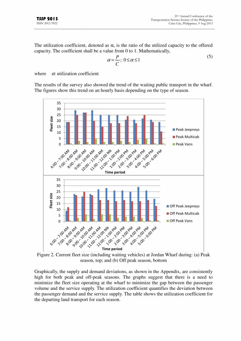
(5) where α: utilization coefficient The results of the survey also showed the trend of the waiting public transport in the wharf. The figures show this trend on an hourly basis depending on the type of season.
Figure 2. Current fleet size (including waiting vehicles) at Jordan Wharf during: (a) Peak
season, top; and (b) Off peak season, bottom Graphically, the supply and demand deviations, as shown in the Appendix, are consistently high for both peak and off-peak seasons. The graphs suggest that there is a need to minimize the fleet size operating at the wharf to minimize the gap between the passenger volume and the service supply. The utilization coefficient quantifies the deviation between the passenger demand and the service supply. The table shows the utilization coefficient for the departing land transport for each season.
�
�
��
��
��
��
��
��
�� ����
��� �� ����
�� ��������
�� � �������
�� ����
�
�
��
��
��
��
��
��
�� ����
��� �� ����
� ���� ��������
� ���� � �������
� ���� ����
1 0 ; ≤≤= αα
CP

�����������������������
����� ��������������������������������������������������������������������������
������������������������� � ������
Table 2. Utilization coefficients (α) for departing land transport
Time period Jeepneys Multicab Vans Peak Off-Peak Peak Off-Peak Peak Off-Peak
6:00 – 7:00 AM 0.16 0.19 0.20 0.10 0.61 - 7:00 – 8:00 AM 0.30 0.36 0.27 0.34 0.47 0.12 8:00 – 9:00 AM 0.51 0.29 0.48 0.31 0.51 0.22 9:00 – 10:00 AM 0.51 0.33 0.55 0.39 0.63 0.15 10:00 – 11:00 AM 0.62 0.27 0.58 0.36 0.67 0.13 11:00 – 12:00 NN 0.52 0.27 0.54 0.31 0.94 0.24 12:00 – 1:00 PM 0.43 0.29 0.45 0.41 0.58 0.28 1:00 – 2:00 PM 0.45 0.27 0.47 0.42 0.63 0.33 2:00 – 3:00 PM 0.53 0.36 0.46 0.52 0.79 0.39 3:00 – 4:00 PM 0.48 0.39 0.40 0.40 0.69 0.69 4:00 – 5:00 PM 0.55 0.48 0.48 0.44 1.00 0.74 5:00 – 6:00 PM 0.62 0.77 0.79 0.58 0.89 1.00 The table shows that the service supply is not fully utilized during the daily operations which could also be attributed to the high number of vehicles waiting at the wharf. It could also be noted further that the utilization coefficients are significantly lower at off-peak seasons. 4.3 Determination of Departing Land Transport Fleet Size The determination of the appropriate fleet size was based on the appropriate passenger design volume. The passenger design volume is derived from the arrivals of pumpboats that were modeled to a Poisson process. The pumpboat operations are also divided into peak and off-peak seasons and further subdivided into peak and off-peak operating hours. The pumpboat frequencies were tested to fit a Poisson distribution at a 95% level of confidence and level of significance α = 0.05. Using SPSS, the data were tested to fit the Poisson distribution using the sample mean as the occurrence rate, λ. The data were validated using the Kolmogorov-Smirnov Test with the following null hypothesis and results from SPSS shown in the succeeding figure.

�����������������������
����� ��������������������������������������������������������������������������
������������������������� � ������
Figure 3. Summary of Distribution Fitting of Pumpboat Frequencies to the Poisson
distribution using SPSS The Poisson distribution determines the probability of an event Xt occurring in an interval (0, t). Mathematically,
(6)
where λ, mean occurrence rate (i.e. the average number of occurrences of the event) With the cumulative distribution function of each season already, the 95% probability of no more than X pumpboats arriving at the wharf were determined. This value enables the researcher to have a confidence that at 95% of the time, there would be no greater frequency than the determined value. In other words, this estimates the maximum value of pumpboat frequency for the different seasons. The results are calculated below in Table 5.
Table 3. Number of Pumpboat Arrivals at 95% Confidence
Condition x. No. of Arrivals Peak season, peak period 26 Peak season, off-peak period 19 Off-peak season, peak period 24 Off-Peak season, off-peak period 16
The passenger demand is the product of the frequency or the number of arrivals for each condition and the capacity of pumpboats, normally forty-five (43). The demand is multiplied to the modal shares, β, to determine the passenger demand for each mode of transport. In case that the design volume for the design hour is less than the vehicle capacity, the design volume is added onto the next hour. The number of vehicles, n, or designed frequency is determined as the quotient of the design volume and the individual capacities of each mode of transport.
(7)
(8)
where, Pd: design volume, β: modal share PdJ,MC,V: design volume for each mode
J - jeepney (cap. 24), MC – multicab (cap. 16) , V – van (cap. 18) n, fd: number of vehicles needed or design frequency CJ,MC,V : capacity for each mode of transport It should be noted that n or the designed frequency assures that all vehicles will depart the wharf for the specific time period. The table shows the proposed fleet size at the wharf. Unlike the current condition, the fleet size proposed in this period is assured of departure within the operating day.
( ) tx
t ext
xXP λλ −==!
)(
β⋅= dd PPTVM CM ,,,
VMCJ
d
d C
Pfn VM CJ
,,
,,==

�����������������������
����� ��������������������������������������������������������������������������
������������������������� � ������
Figure 4. Proposed fleet size (including waiting vehicles) at Jordan Wharf during: (a) Peak
season, top; and (b) Off peak season, bottom
In correspondence to the proposed number of waiting vehicles, the effect of the proposal to the utilization coefficient was made and shown in Table 6. It can be noted that majority of the coefficients improved from the current condition. Likewise, across all time periods, all of the utilization coefficients were above 0.5 which implies that the utilized capacity is about 50% of the total offered capacity which makes the operations more efficient. There are time periods that the coefficients are greater than 1.0. With this high utilization coefficient, transit operators can increase the number of frequency or increase the number of waiting vehicles. As much as possible, utilization coefficients should not exceed the value of 1 to avoid crowding inside the vehicle. Increasing the frequency in this case would not constitute an immediate effect to the operations of the wharf but, it would give passengers more comfort inside the vehicle.
�
�
��
��
��
��
�� ����
��� �� ����
�� ��������
�� � �������
�� ����
�����
������������
�� ����
��� �� ����
� ���� ��������
� ���� � �������
� ���� ����

�����������������������
����� ��������������������������������������������������������������������������
������������������������� � ������
Table 4. Utilization coefficients (α) of proposed condition
Time period Jeepneys Multicab Vans Peak Off-Peak Peak Off-Peak Peak Off-Peak
6:00 – 7:00 AM 1.07 1.01 1.00 1.01 1.01 - 7:00 – 8:00 AM 1.03 1.02 1.08 1.14 1.85 1.14 8:00 – 9:00 AM 1.05 1.06 1.04 1.08 1.40 - 9:00 – 10:00 AM 1.01 1.07 1.05 1.05 1.24 1.14 10:00 – 11:00 AM 1.00 1.08 1.00 1.06 1.39 - 11:00 – 12:00 NN 1.04 1.04 1.02 1.00 1.22 1.50 12:00 – 1:00 PM 1.04 1.03 1.11 1.05 1.84 1.55 1:00 – 2:00 PM 1.02 1.03 1.02 1.00 1.25 1.05 2:00 – 3:00 PM 1.03 1.04 1.04 1.07 1.07 1.02 3:00 – 4:00 PM 1.05 1.07 1.01 1.02 1.30 1.23 4:00 – 5:00 PM 1.06 1.04 1.06 1.06 - - 5:00 – 6:00 PM 1.00 1.05 1.06 1.03 - - 4.4. Data Validation To validate if there was a significant difference to the current and the proposed conditions, a t-test was performed on the fleet size. A paired t-test was perform with the null hypothesis is that there is no difference between the two means (H0 - H1 = 0) while the alternative hypothesis is that the two means are not equal. The statistical results are shown in the next tables.
Table 5. Paired T-test Results for: (a) Jeepney, (b) Multicab, and (c) Van J_PREV_P J_PROP_P J_PREV_OP J_PROP_OP
Mean 23.583333 15.66666667 23.5 13.25 Variance 12.810606 15.15151515 29.18181818 12.56818182 t Stat 9.054154 6.664377776 P(T<=t) two-tail 1.977E-06 3.54183E-05 t Critical two-tail 2.2009852 2.20098516
MC_PREV_P MC_PROP_P MC_PREV_OP MC_PROP_OP Mean 19.91666667 12.75 18.08333333 10.75 Variance 21.35606061 6.20454545 13.17424242 7.477272727 t Stat 6.321292798 4.976222533 P(T<=t) two-tail 5.66671E-05 0.000417927 t Critical two-tail 2.20098516 2.20098516
V_PREV_P V_PROP_P V_PREV_OP V_PROP_OP Mean 2.583333 1.833333 3.333333 1.833333 Variance 2.083333 1.606061 3.69697 2.515152 t Stat 5.744563 2.569047 P(T<=t) two-tail 0.000129 0.026095 t Critical two-tail 2.200985 2.200985

�����������������������
����� ��������������������������������������������������������������������������
������������������������� � ������
With the p-values less than 0.05 the results are significant at a 5% level of significance. The t-stat is also greater than the critical t-value for two-tailed test which shows that there is a significant difference between the current and the proposed conditions. 5. CONCLUSIONS The result of this paper showed that there is an oversupply of public transportation at the Jordan wharf. The oversupply of public transport leads to a very small utilization coefficients for departing public transport as there are a lot of vehicles that are waiting at the wharf. The waiting vehicles have no effect on the arriving public transport at the wharf. The results show that there is still a need for improvement in increasing the coefficient for departing public transport. The methodology presented, using the frequency of arrivals of pumpboats modeled after a Poisson distribution, is an effective tool as it considers the seasonal and hourly variations of the passenger demand. A more in-depth methodology of vehicle scheduling considering the actual routes of each mode of transport is suggested to further increase utilization of public transport modes. The resulting proposed utilization coefficients are mostly above 1.0. The values imply that there is a need to increase the fleet size to avoid overcrowding. Hence, the proposed fleet size considered is the minimum fleet size that would address the arriving passengers.
ACKNOWLEDGEMENT
The researchers would like to thank the Engineering Research for Development and Technology (ERDT) of the Department of Science and Technology (DOST) for funding this research. The researcher would also like to extend his gratitude to the students of Central Philippine University in Iloilo for their assistance in the conduct of this research. The researchers are also grateful for the assistance of Engr. Evan Arias of the Provincial Planning and Development Office of the Provincial Government of Guimaras.
REFERENCES Ang, A. & Tang, W. (2007) Probability Concepts in Engineering: Emphasis on Applications on Civil & Environmental Engineering. Wiley, New Jersey Ceder A. (1984) Bus frequency determination using passenger count data. Transportation Research – Part A 18 (5-6), 439 – 453 Ceder A. (2007). Public Transit Planning and Operation: Theory, modeling and practice. Butterworth – Heinemann Furth, P. G., & Wilson, N. H. M. (1982) Setting frequencies on bus routes: Theory and practice. Transportation Research Record 818, 1-7 Henry, L., & Marsh, D. L. (2008). Intermodal surface public transport hubs: Harnessing synergy for success in America’s urban and intercity travel. American Public Transportation Association (APTA) Bus and Paratransit Conference, Austin, USA.

�����������������������
����� ��������������������������������������������������������������������������
������������������������� � ������
Jones, W. B., Cassady, C. R., & Bowden, R. O. (2000). Developing a standard definition of intermodal transportation. Transportation Law Journal 27, USA Kang, H. A., Mascarina, K. B., & Padua, M. J. (2011). Proposed scheduling of Jeepney operations in Malate Area, Thesis (BS Civil Engineering – Transportation Engineering), De La Salle University – Manila Litman, T. (2009). Introduction to Multi-Modal Transportation Planning. Victoria transport policy institute, Canada Pitsiava-Latinopoulou, M., & Iordanopoulos, P (2012). Intermodal passengers terminals: Design standards for better level of service. Procedia – Social and Behavioral Sciences 48, 3297-3306 Rivasplata, C. R. (2001). Intermodal transport centers: towards establishing criteria. 20th South African Transport Conference. Vuchic, V. (2005). Urban Tansit: Operations, planning, and economics. Wiley

�����������������������
����� ��������������������������������������������������������������������������
������������������������� � ������
APPENDIX
Figure A.1 The Demand and Supply Difference in Jeepneys during (a) Peak and (b) Off-Peak Seasons
�
���
���
���
���
���
���������
���������
���������
���������
���������
���������
���� ���
���� ���
�����������
�����������
�����������
�����������
�����������
�����������
���������
���������
���������
���������
���������
���������
���������
���������
���������
���������
� ��
��� �����!�"#$��% � &'����
�
���
���
���
���
���
���
���������
���������
���������
���������
���������
���������
���� ���
���� ���
�����������
�����������
�����������
�����������
�����������
�����������
���������
���������
���������
���������
���������
���������
���������
���������
���������
���������
� ��
��� �����!�"#$��% � &'����
���
������������������
���������
���������
���������
���������
���������
���������
���� ���
���� ���
�����������
�����������
�����������
�����������
�����������
�����������
���������
���������
���������
���������
���������
���������
���������
���������
���������
���������
� ��
��� �����!�"#$��% � &'����

�����������������������
����� ��������������������������������������������������������������������������
������������������������� � ������
Figure A.2 The Demand and Supply Difference in Multicabs during (a) Peak and (b) Off-Peak Seasons
Figure A.3 The Demand and Supply Difference in Vans during (a) Peak and (b) Off-Peak Seasons
���
������������������
���������
���������
���������
���������
���������
���������
���� ���
���� ���
�����������
�����������
�����������
�����������
�����������
�����������
���������
���������
���������
���������
���������
���������
���������
���������
���������
���������
� ��
��� �����!�"#$��% � &'����
�
��
��
��
��
��
���������
���������
���������
���������
���������
���������
���� ���
���� ���
�����������
�����������
�����������
�����������
�����������
�����������
���������
���������
���������
���������
���������
���������
���������
���������
���������
���������
� ��
��� �����!�"#$��% � &'����
�
��
��
��
��
���
���
���������
���������
���������
���������
���������
���������
���� ���
���� ���
�����������
�����������
�����������
�����������
�����������
�����������
���������
���������
���������
���������
���������
���������
���������
���������
���������
���������
� ��
���
�����!�"#$��% � &'����