IMPROVED SPECTRAL PARAMETERS FOR THE THREE MOST …

.I. Quant. Spcctrosc. Radiat. Transfer Vol. 59. No. 35, pp. 495-509. 1998 0 1998 Elsevier Science Ltd. All rights reserved Pergamon

PII: SOO224073@7)00124-6 Printed in Great Britain

0022-4073/98 619.00 + 0.00

IMPROVED SPECTRAL PARAMETERS FOR THE THREE MOST ABUNDANT ISOTOPOMERS OF THE OXYGEN

MOLECULE

ROBERT R. GAMACHE,t$ AARON GOLDMAN8 and LAURENCE S. ROTHMANII

TDepartment of Environmental, Earth, and Atmospheric Sciences, University of Massachusetts Lowell, 1 University Avenue, Lowell, MA 01854, U.S.A., §Department of Physics, University of

Denver, Denver, CO 80208, U.S.A. and I(AF Geophysics Directorate, 29 Randolph Road, Hanscom AFB, Hanscom, MA 01731, U.S.A.

Abstract-Line positions, intensities, transition-moment squared, and lower state energies are calculated for the three most abundant isotopomers of the oxygen molecule in the terrestrial atmosphere, 1602, ‘80’60, and ‘70’60. All lines passing a wavenumber dependent cutoff procedure (3.7 x lo-” cm-‘/(molecule cm-‘) at 2000 cm-‘) are retained for the 1996 HITRAN database. Halfwidths as a function of the transition quantum numbers are determined from the available experimental measurements. Explicit expressions are obtained relating line intensities to the transition-moment squared, the vibrational band intensity, and the electronic-vibrational Einstein-A coefficient. The statistical degeneracy factors are presented and misuse of these factors in previous works is explained. Finally, band-by-band comparisons between the new calculations and the data from the previous HITRAN database are made. 0 1998 Elsevier Science Ltd. All rights reserved

1. INTRODUCTION

Atmospheric spectra of oxygen are used for deducing information about properties and other species in the atmosphere, for example, measurements of 0, emission are used as a standard for 0, profile analysis.‘,* There is a need to have available the most accurate parameters for this molecule. The spectrum of the oxygen molecule, even though O2 is a simple diatomic, is unexpectedly complex. The oxygen molecule has two unpaired electrons with a total spin of 1 in the electronic ground state. There are two low-lying excited electronic states which give rise to near-I.R. and visible spectra, and the symmetries of the isotopomers, 1602, ‘60’80, and ‘60’70, affect the number of allowed states. In addition, both magnetic dipole and electric quadrupole transitions occur, the degeneracy of states needs to be carefully considered, and transitions occur from the microwave to the visible. Although the line intensities are usually small, the high mixing ratio and long optical path in the terrestrial atmosphere compensate to produce meaningful absorption.3

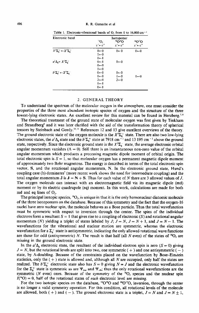
In this work, the spectral parameters for the oxygen molecule are calculated for the electronic-vibrational bands listed in Table 1. These data represent an improvement to the data contained on the 1992 version of the HITRAN molecular absorption database,4 which are from calculations made in 1982.5 The calculations consider the lower state energy, the wavenumber of the transition, the line intensity, and transition moment squared of the spectral lines. In addition, halfwidths as a function of transition quantum number are determined from the available experimental measurements. All fundamental physical constants used in the calculations are those reported by Cohen and Taylor.6 The calculations were made in double precision on several different computer systems using codes written in FORTRAN. Below, we discuss the theory of molecular oxygen and describe the improvements to the data for each band.

fTo whom all correspondence should be addressed.

496 R. R. Gamache et al

Table 1. Electronic-vibrational bands of O2 from 0 to 16,000 cm- ’

Electronic band Isotopomer ‘60, ‘60’80 MO”0

v~cy” 7,1,cu1* u’tL”’

X’Z, cx’z, oco 04-O oco I+0 I-1

a’A,tX’X; O+l oto O+O I+0

b’&+ tn, o-0 O+O I+0 I-0 I+0 2to 2-O IS-1 0-l

2. GENERAL THEORY

To understand the spectrum of the molecular oxygen in the atmosphere, one must consider the properties of the three most abundant isotopic species of oxygen and the structure of the three lowest-lying electronic states. An excellent review for this material can be found in Herzberg.‘.*

The theoretical treatment of the ground state of molecular oxygen was first given by Tinkham and Strandberg and it was later clarified with the aid of the transformation theory of spherical tensors by Steinbach and Gordy.“*” References 12 and 13 give excellent overviews of the theory. The ground electronic state of the oxygen molecule is the X’C, state. There are also two low-lying electronic states, the a’ A, state and the b’E:,+ state at 79 18 cm - ’ and 13 195 cm - ’ above the ground state, respectively. Since the electronic ground state is the X’E; state, the average electronic orbital angular momentum vanishes (A = 0). Still there is an instantaneous non-zero value of the orbital angular momentum which produces a precessing magnetic dipole moment of orbital origin. The total electronic spin is S = 1, so that molecular oxygen has a permanent magnetic dipole moment of approximately two Bohr magnetons. The energy is described in terms of the total electronic spin vector, S, and the rotational angular momentum, N. In the electronic ground state, Hund’s coupling case (b) dominates’ (more recent work shows the need for intermediate coupling) and the total angular momentum J is J = N + S. Thus for each value of N there are 3 allowed values of J. The oxygen molecule can interact with an electromagnetic field via its magnetic dipole (md) moment or by its electric quadrupole (eq) moment. In this work, calculations are made for both md and eq lines of 0,.

The principal isotopic species, 1602, is unique in that it is the only homonuclear diatomic molecule of the three isotopomers on the database. Because of this symmetry and the fact that the oxygen-16 nuclei have zero nuclear spin, the molecule behaves as a Bose particle. Thus the total wavefunction must be symmetric with respect to inversion through the center. The spins of the individual electrons form a resultant S = 1 that gives rise to a coupling of electronic (S) and rotational angular momentum (N) yielding a triplet of states labeled by J; J = N, J = N + 1, and J = N - 1. The wavefunctions for the vibrational and nuclear motion are symmetric, whereas the electronic wavefunction for a C, state is antisymmetric, indicating the only allowed rotational wave functions are those for odd (antisymmetric) N. The result is that half (all N even) of the states of 1602 are missing in the ground electronic state.

In the a’A, electronic state, the resultant of the individual electron spin is zero (S = 0) giving J = N, but the rotational levels are split into two, one symmetric ( + ) and one antisymmetric ( - ) state, by A-doubling. Because of the constraints placed on the wavefunction by Bose-Einstein statistics, only the ( + ) state is allowed and, although all N are occupied, only half the states are realized. The 6%: electronic state also has S = 0 giving N = J and the electronic wavefunction for the Cl state is symmetric as are Y’,,, and ‘I’v’b; thus the only rotational wavefunctions are the symmetric (N even) ones. Because of the symmetry of the 1602 species and the nuclear spin Z(160) = 0, half of the rotational states of each electronic level are missing.

For the two isotopic species on the database, ‘60’80 and ‘60’70, inversion, through the center is no longer a valid symmetry operation. For this condition, all rotational levels of the molecule are allowed, both ( + ) and ( - ). The ground electronic state is a triplet, .Z = N and .Z = N + 1,

Improved parameters for isotopmers of oxygen 497

with all N allowed, N = 1, 2, 3, . . . . The two low-lying electronic states, a’A, and b’&+ are singlets (J = N) with all values of N (even and odd) starting at N*i” = A. Note that for the a’A, state there is A-type doubling, thus each N has two states.

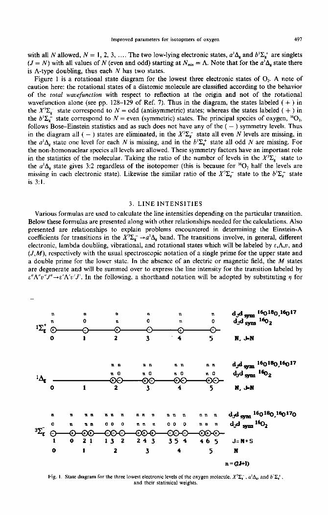
Figure 1 is a rotational state diagram for the lowest three electronic states of 0,. A note of caution here: the rotational states of a diatomic molecule are classified according to the behavior of the total wavefunction with respect to reflection at the origin and not of the rotational wavefunction alone (see pp. 128-129 of Ref. 7). Thus in the diagram, the states labeled ( + ) in the X3X, state correspond to N = odd (antisymmetric) states; whereas the states labeled ( + ) in the PC,+ state correspond to N = even (symmetric) states. The principal species of oxygen, 1602, follows Bose-Einstein statistics and as such does not have any of the ( - ) symmetry levels. Thus in the diagram all ( - ) states are eliminated, in the X’C, state all even N levels are missing, in the a’A, state one level for each N is missing, and in the b’C,f state all odd N are missing. For the non-homonuclear species all levels are allowed. These symmetry factors have an important role in the statistics of the molecular. Taking the ratio of the number of levels in the X’C, state to the a’A, state gives 3:2 regardless of the isotopomer (this is because for 1602 half the levels are missing in each electronic state). Likewise the similar ratio of the X3X- state to the b’&+ state is 3:l.

3. LINE INTENSITIES

Various formulas are used to calculate the line intensities depending on the particular transition. Below these formulas are presented along with other relationships needed for the calculations. Also presented are relationships to explain problems encountered in determining the Einstein-A coefficients for transitions in the X3&- +a’4 band. The transitions involve, in general, different electronic, lambda doubling, vibrational, and rotational states which will be labeled by e,A,v, and (J,M), respectively with the usual spectroscopic notation of a single prime for the upper state and a double prime for the lower state. In the absence of an electric or magnetic field, the M states are degenerate and will be summed over to express the line intensity for the transition labeled by &“A”L~“J”~E’A’v’J’. In the following, a shorthand notation will be adopted by substituting r] for

n n n n n n d&m 1~180,16@7

,” “_ dJb= ‘602

v V

0 1 2 3 ~ 4 5 N. J-N

nn nn nn nn dJ%= 1~1~,16017

‘4 UO UO UO IlO ‘J’,, 1602

0 1 2 3 4 5 N, .bN

II II nn nn n nn n nn n nn n dJdsym 16~18~,16@7~

160,

1 0 21 13 2 24 3 35 4 46 5 J=N+S

0 1 2 3 4 5 N

n = (2J+l)

Fig. 1. State diagram for the three lowest electronic levels of the oxygen molecule, X3X;, a’A,, and b’&+ and their statistical weights.


the set of quantum numbers EAuJ. Thus q” = s”A”v”J” and q’ = E’A’v’J’. The line intensity in units of (cm -‘/molecule cme2) for a transition q”+ is (see Refs. 14 and 15)

where the total internal partition sum, Q(T), is

Q(T) = 2 d,d,,dvd,dsyme - ‘s.&~’ , Ehl'J

(2)

and J, is the isotopic abundance of the species, the factor lO-“j is needed for the units chosen. IR~E”~r”l”~.HE.A.C.J.M.) I2 is the transition-moment squared and has units of Debye2/molecule, d,,” is the degeneracy and E,*, the energy of the state q”, v~,,~~~~,,~~/c = Ok,,,) is the wavenumber of the transition, and all other variables are the usual constants. (Note, in Eq. (1) and in a few expressions that follow we have not canceled some of the degeneracy factors in order to emphasize the fractional number of molecules in the state q”, N,..) In this paper we use the ‘regular’ matrix elements while in the Gamache and Rothman (1992) paper’5 we used the ‘weighted’ ones. The degeneracy factors are given by the product of the degeneracy factors for the quantized motions, d,, = d,dvd,dsy, with d, = (2s + l), d,, = (2 - 6,,0), d, = 1, d, = (25 + I), and dsym is one for the heteronuclear species and the ( + ) states of the homonuclear species and zero for the ( - ) states of the homonuclear species. This factor accounts for the symmetry restrictions for the homonuclear diatomics (note, this gives an overall factor of l/2 in the partition sum).

This expression can be written in terms of the Einstein-A coefficient by making use of the relationshipi

A 64n4 1O-36

4’~9” = 3h

whence the line intensity is

(3)

(4)

The Einstein-A coefficient is usually determined from a measurement of a vibrational band intensity, S::,$y so it is useful to formulate Eq. (1) and Eq. (4) in terms of this quantity. The integrated intensity for an electronic-vibration-rotation band in units of cm - ‘/(molecule cm- ‘) is given byI

S d,,w,,m _ 87r3 10 - 36 iI\‘V’ - 3hc (5)

(Note, this is similar to a/N, (Ref. 14, p. 153 with a = ~I’IS~,,A”V”J”_~.h.v,l.) with the exception that the radiation field term, (1 - e - ‘“(q”~q,d~‘), is explicitly retained in the rotational part of the intensity formula. Thus our definition of S:r,^::: does not contain the approximate factor (1 - e - hv(~-~.~~n~~~~~~‘k3.) To implement Eq. (5), the electronic-vibration and rotation parts are separated using the product approximation for the total partition sum and the transition-moment squared, and the assumption of additivity of energy


E,,” = EE,.,,“p.. + Er.

Inserting these into Eq. (1) and rearranging terms yields

(7)

The first part of this expression is simply the band intensity intensity can be written

In what follows we will need the relationships between electronic-vibrational transition-moment squared. They are

- e - hYwn4 )lkT >

I&,mH,,,12.

as defined in Eq. (5); thus the line

e - %~II )jk7 >

lJ&,,,l* . (8)

the Einstein coefficients and the

B EIIIZllyl_E,A,“, = 8x33; - 36 IR,c”h..““)(c.iZ.“.~l* ,

B EII\lyl_E,.I\I”,I =

and

A. 641~’ 1O-36

F ,4’V’-t~“A-V” = 3h

Solving Eq. 9c for the transition-moment squared and inserting into Eq. (5) gives the result

This expression allows the Einstein-A coefficient to be determined by measuring the integrated band intensity. This relationship with Eq. (8) allows the &“A”v”J” +.s’A’z)‘J’ line intensity to be written in terms of the Einstein AEI,,.V..+E..hrcV.. coefficient

(11)

where the partition function and the energy are no longer approximated and the Honl-London factor is inserted for the rotational transition-moment squared. Note that the degeneracy factors preceding the Einstein-A coefficient account for the number of J and M states in the upper and lower electronic-vibration states and the degeneracy factors with the partition function term are d,,,,, = (2s + 1)(2 - 6,,,O)(d,,,)(2 J + 1). From the symmetry arguments presented above, it is clear that the ratio of the degeneracy factors, d~.,,.y~/de..~_v.., is 213 for X’C, +a’A, transitions and l/3 for the X3X, -+b’C,f transitions.

For several of the bands calculated, the program employs the Einstein-A coefficients in units of set-‘. Often one must work from measured vibrational band intensities. In order to make use of these values, we must convert from vibrational band intensity to the Einstein-A coefficient. This relationship was presented in Eq. (10). However, quite often in the literature the vibrational band intensity is reported in units of cm - ’ km - ’ atm - ’ STP. The values must be converted to the


HITRAN units of cm - ‘/(molecule cm - ‘) to apply the equations presented here. This is accomplished by the relationship

S:. cm-’

>

NL molecule cm - 2 x p(atm)

x lo5 E = S;(cm - ‘km - ‘atm - ‘STP) (12)

where NL is Loschmidt’s number, the number of molecules per cubic centimeter of perfect gas at STP. Thus we have

s:. cm-’ molecule cm - 2

x 2.6867 x 1024E = S:(cm-'km-'atm-'STP) . (13)

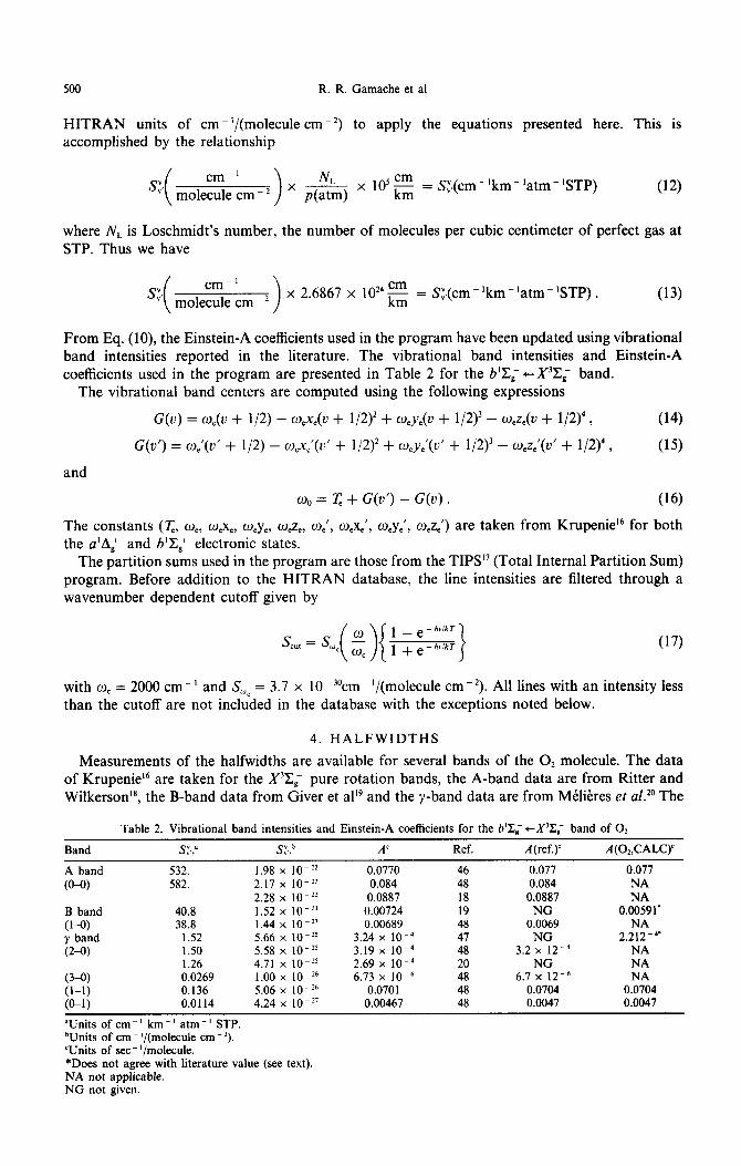
From Eq. (lo), the Einstein-A coefficients used in the program have been updated using vibrational band intensities reported in the literature. The vibrational band intensities and Einstein-A coefficients used in the program are presented in Table 2 for the b’C: +X3X, band.

The vibrational band centers are computed using the following expressions

G(v) = o,(u + l/2) - w,xe(u + 1/2)2 + w,y,(u + 1/2)3 - o,ze(v + 1/2)4, (14)

G(o’) = w:(v’ + l/2) - o>~‘(u’ + l/2)* + oeve’(u’ + 1/2)3 - w,z,‘(u’ + 1/2)4, (15)

and

o0 = r + G(v’) - G(u) . (16)

The constants (T_ w,, 0,x,, meye, w,z,, CD,‘, w,x,‘, meye’, w,z,‘) are taken from Krupenie16 for both the a’A: and b’C,+ electronic states.

The partition sums used in the program are those from the TIPS” (Total Internal Partition Sum) program. Before addition to the HITRAN database, the line intensities are filtered through a wavenumber dependent cutoff given by

(17)

with W, = 2000 cm - ’ and So,, = 3.7 x 10 - 3ocm - ‘/(molecule cm - “). All lines with an intensity less than the cutoff are not included in the database with the exceptions noted below.

4. HALFWIDTHS

Measurements of the halfwidths are available for several bands of the 0, molecule. The data of Krupenie16 are taken for the X3X, pure rotation bands, the A-band data are from Ritter and Wilkerson”, the B-band data from Giver et alI9 and the y-band data are from MClihes et al.” The

Table 2. Vibrational band intensities and Einstein-A coefficients for the 6%: +X’Z; band of 0,

Band A’ Ref. A(ref.)’ A(O,,CALC)

A band 532. 198 2:17

x lo-z2 (M) 582. x 10-j’

228 x lo-” B band 40.8 152 x lo-= (1-o) 38.8 1.44 x 10-Z’ y band 1.52 5.66 x 1O-z5 (2-o) 1.50 5.58 x lo-*’

1.26 4.71 x lo-?5 (3-O) 0.0269 1.00 x 1o-26 (1-I) 0.136 5.06 x 1O-26 (Gl) 0.0114 4.24 x lo-”

“Units of cm-’ km-’ atm- ’ STP. ‘Units of cm - ‘/(molecule cm - 2). ‘Units of set - ‘/molecule. *Does not agree with literature value (see text). NA not applicable. NG not given.

0.0770 46 0.077 0.077 0.084 48 0.084 NA 0.0887 18 0.0887 NA

0.00724 19 NG 0.00591’ 0.00689 48 0.0069 NA

3.24 x 1O-4 47 NG 2.212-4’ 3.19 x 1o-4 48 3.2 x 12-4 NA 2.69 x 1O-4 20 NG NA 6.73 x lO-6 48 6.7 x l2-6 NA

0.0701 48 0.0704 0.0704 0.00467 48 0.0047 0.0047


A-band PP transitions, Ref. 18 A-band PQtransitions, Ref. 18 A-band RRtmnsitions, Ref. 18 A-band RQtransitions, Ref. 18 @and PP transitions, Ref. 20 y-band PP transitions, Ref. 20 B-band PP transitions, Ref. 19 B-band PQtransitions, Ref. 19 B-band RR transitions, Ref. 19 B-band RQtmnsitions, Ref. 19

0.035-r 7 . . . I . . . . I . * ’ . I 7 . . . 1 . . . . , . . . 0 5 10 15 20 25 30

N”

Fig. 2. Halfwidth data cm-’ atm- ’ at 296 K for the A-, B- and 7 bands of O2 according to branches as a function of N.

data of Refs. 18-20 are plotted in Fig. 2 as a function of N” for the various types of transitions. The transitions are labeled by ANAJ IV” J”; however with symmetry arg~ents the notation dNAJN’f is often used. For the A-band we find that if the RR and RQ values are shifted,

(N”+N” + 2)? they agree with the ‘P and ‘Q values (see Fig. 3), i.e.,

Y( ‘P,-) = Y( R&,, + 2)

__

0.065

A-Band Data from Ref. 18 4 3 - PP transitions

- FQ transitions

jj 0.055- ---*--- RR transitions

T - RQ transitions

&

2

F 0045- x *

QO35:-..‘,.--.r..‘-l-...,“..,*-,. 0 5 10 15 20 25 30

N

Fig. 3. A-band halfwidths cm-’ atm-’ at 296 K, RR and RQ values are shifted, N”-+N” + 2

JQSRT59f 5 M


and

Y( ‘Qw) = 14 “Qw+J (18)

For the B-band, the difference between the ‘P, PQ,RR, and RQ values for a given N” is small. The data of Mel&es et al” for the y-band, however, show large variations in the halfwidth as a function of N” not seen in the other data (see open circles and triangles in Fig. 2).

Comparing the values from Refs. 18-20, we find that the A- and y-band results agree with each other and the B-band results are some 10% larger. The data selected for 0, on the 1996 HITRAN database use the following procedure for the halfwidths. The X’C, pure rotation band uses the data reported by Krupenie I6 for the 60 GHz lines. The electric quadrupole transitions and the transitions involving the a’A, state use the A-band values.” For the A- and y-bands, the halfwidths of Ritter and Wilkerson’* are averaged as a function of N” for the ‘P and ‘Q lines together and the RR and RQ lines together. We have calculated transitions to N” = 80 and the measurements end at N” = 29; thus it is necessary to extrapolate the data. From the plots, an asymptotic limit of y = 0.032 cm- ‘/atm for N” 2 40 is estimated. Both the R and P lines use the same asymptotic limit. The values of the halfwidths for the A- and B-bands of O2 used in the HITRAN are given in Table 3.

5. UPDATES TO THE OXYGEN DATA FOR THE 1996 HITRAN DATABASE

Below, the changes made to the data for the 1996 HITRAN database are discussed for each band of molecular oxygen considered. The line position and energy differences are defined as the HITRAN value minus the HITRAN value. For the line intensities the ratio computed is HITRAN92/HITRAN96. The average and maximum differences were calculated for the line position and energy parameters. For the line intensities, the average, maximum and minimum ratios were calculated.

5.1. The principal isotopic species, ‘602

51.1. The X3&- (u = 0)t X3&- (2’ = 0) band. The energy levels for the vibrational ground state of the X’C, electronic state of 1602 are calculated using the formalism of Rouille et al.*’ In this work the Hamiltonian included all rotational terms to second order** and some terms to third order.23. 24 The molecular constants are those of Rouille et al.*’ These are compared with the energy values from the previous database (the energy levels for 0, on the 1982-1992 versions of HITRAN

Table 3. Halfwidths in cm- ‘iatm for the A- and B-bands of 0,

N”

1

A - P’

0.0592

A - R’

0.0587

B”

0.0616

N” A - P’ A - R: Bh

21 0.0417 0.0406 0.0454 2 0.0574 0.0562 0.0600 22 0.0409 0.0402 0.0447 3 0.0557 0.0538 0.0584 23 0.0402 0.0397 0.0440 4 0.0544 0.0523 0.0571 24 0.0395 0.0386 0.0436 5 0.053 1 0.0509 0.0558 25 0.0389 0.0376 0.0432 6 0.0520 0.0503 0.0555 26 0.0380 0.0371 0.0428 7 0.0509 0.0498 0.0552 27 0.0371 0.0366 0.0422 8 0.0502 0.0492 0.0547 28 0.0365 0.0183 0.0418 9 0.0495 0.0486 0.0541 29 0.0358 0.0358 0.0414 10 0.0488 0.0479 0.0531 30’ 0.0353 0.0353 0.0410 11 0.0482 0.0473 0.0521 31’ 0.0349 0.0349 0.0407 12 0.0475 0.0467 0.0515 32’ 0.0345 0.0345 0.0404 13 0.0468 0.046 1 0.0509 33’ 0.0340 0.0340 0.0400 14 0.0464 0.0455 0.0504 34’ 0.0337 0.0337 0.0398 15 0.0459 0.0449 0.0499 35’ 0.0334 0.0334 0.0395 16 0.0452 0.0441 0.0488 36‘ 0.0330 0.0330 0.0394 17 0.0445 0.0432 0.0477 37’ 0.0328 0.0328 0.0393 18 0.0438 0.0426 0.0469 38’ 0.0324 0.0324 0.0391 19 0.043 1 0.0421 0.0461 39’ 0.0322 0.0322 0.0390 20 0.0424 0.0413 0.0457 40’ 0.0320 0.0320 0.0390

‘A-band ‘P and ‘Q transitions. *A-band ‘R and “Q transitions. *B-band transitions. ‘Extrapolated.

Improved parameters for isotopmers of oxygen

xmmm* mm+ n 4 X4 x’++

XI’+ x4++

X n 4

++

I. + ‘+

x, +

l

x J=N+l X l

l J=N X

+ J=N-1 x

II -6.3 ; . . - * I . . . . * 1. . . . . I . . . . . I * . . . . I . . . . . I . . - . . I . . . ’ .

0 10 20 30 40 66 60 70

N

503

Fig. 4. Energy difference in cm - ’ between the formalism of Rouille et al*’ and Greenbaum’) vs N for the rn = 0 states of X3&- of ‘60z.

used for the formulation of Ref. 13) in Fig. 4. The difference in energy between the two formulations is given as a function of N and J. For the vibrational ground state the difference is near zero for N up to 35, then rapidly goes to - 0.3 cm-’ at N = 80. While the transition frequencies from this formulation differ only slightly from the previous results, 0.0039 cm-’ maximum difference, 7 x 10 - 5 cm - ’ on average, the formalism of Rouille et a12’ gives better agreement with measurements.1

This band has both magnetic dipole and electric quadrupole transitions. For the electric quadrupole transitions, a newer value of the quadrupole moment derived from far-IR PIA spectra,25 0.34 x lO-26 esu cm’, has been adopted. There are no data to validate the intensities we obtain. With this value for the quadrupole moment, the line intensities and transition-moments squared are a factor of 5.8 weaker than previous calculations. 26 Because of this reduction in the line intensities, no electric quadrupole lines survived the cutoff for the 1996 data set. This is further discussed below for the 1 CO vibrational band of this electronic band. The 1996 calculations of the magnetic dipole intensities are on average 4% stronger than the 1992 values. This is due to improved energy formulation and partition sums.

5.1.2. The X3&- (tl = 1)~ X’C, (u = 0) band. The 1992 HITRAN database contained only electric quadrupole (eq) lines for this band. The newer data contain both magnetic dipole (md) and electric quadrupole (eq) transitions. 27 Thus, the comparison made here is for the electric quadrupole lines. The energy levels for the vibrational ground (v = 0) and the first fundamental (u = 1) of the X3x; electronic state of 1602 are calculated using the formalism and constants of Rouille et al.” These energies are compared with the values from the previous databases in Fig. 5 for the 0” = 1 states. The difference is small for N up to x 20 then quickly goes to roughly 5 cm ’ at N = 80. For the transitions that make the cutoff criterion, N 5 31, the maximum difference in the energy values is 0.0024 cm -I, 0.0005 cm - ’ on average. The corresponding average and maximum differences in the line positions are - 0.0104 and 0.0850 cm-‘. The electric quadrupole transition line intensities are calculated using the formalism of Goldman et al. 27 The absolute intensities are determined by scaling the relative intensities to the measurements of Reid et al.28 Comparison of these intensities with the 1992 HITRAN values implies an electric quadrupole moment of

SComparisons were made with the data from Refs. 20 and 32. The different formulations are compared with experiment for 30 lines measured in Ref. 32 and for 2 transitions measured in Ref. 20. The comparison shows the Rouillt et al formalism to be very slightly better than that of Ref. 13, with the average deviations being 0.00256 cm-’ vs. 0.00259 cm-‘. respectively. Note the average deviation is deceptive in that most of the deviations comes from a few large lines. However on a line-by-line basis the Rouillt et al data are slightly better than the calculations of Ref. 13.


-

5>

Fig. 5. Energy difference in cm _ ’ between the formalism of Rouillt et al*’ and Greenbaumi3 vs N for the v” = 1 states of X3&- of 160,.

0.145 x 10ez6 esu cm’, not in agreement with the quadrupole moment derived from far-I.R. PIA spectraz5 (see previous section). This is under investigation. Comparing the 1996 and 1992 values for the intensities we find an average ratio of 1.0027, with some ratios between 0.740 and 1.31. These large ratios occur for 33 out of the 146 lines and occur only for forbidden (weaker) lines, with AN # AJ and at low J.

The 1996 calculations for this band are not filtered through a cutoff procedure and many of the lines will have very small intensities. (In fact, one zero intensity magnetic dipole and electric quadrupole transition have been retained in the data for theoretical considerations; it helps to see the effects of assumed parameters on these lines.) There are 254 md transitions and 183 eq transitions retained for this band.

5.1.3. The X’C, (u = 1)~ X’C; (a = 1) band. As discussed above, the energy differences from the previous calculations and the formulation of Rouillt et al*’ for the u = 1 level approach 5 cm - ’ at N = 80. The maximum energy difference in the lines in the 1996 data is 0.750 cm-’ and the average difference is - 0.0953 cm - ‘. The maximum difference in line positions is 0.0457 cm - ’ with the average difference being - 0.00280 cm - ‘. The intensity ratios are between 0.994 and 0.988 with an average ratio of 0.990. Most of this difference comes from using an improved partition sum in the calculations.

5.1.4. The a’d, (u = 0)t X3x8- (u = 0) band. There are wavenumber differences which arise from a change in the energy formulation of X3x:, (u = 0) to that of Rouille et a12’ and for a’b, (u = 0) to that of Scalabrin et a129 with the constants of Hillig et a1.3o The maximum difference is 0.0160 cm-’ at N” = 37 and the average difference is - 0.00234 cm-‘.

The line intensities for this band are calculated using Eq. (11). There are three measurements of the band intensity in the literature (scaled to 296 K) which differ by a factor of about 4.5. The measurement of Badger et a13’ gives S, = 3.6 x lo-” cm-‘/(molecule cm-*). The measurement of Lin et a132 is S, = 9.4 x 10 -24 cm - ‘/(molecule cm - *), and Hsu et a133 report a value of S, = 2.1 x 10 -24 cm -‘/(molecule cm - ‘). From these values the authors determine the Einstein-A coefficient. Unfortunately, some of the authors have used incorrect statistical degeneracy factors, d,/d,; Badger et a13’ used 3/2 whereas Lin et al)* and Hsu et a133 use 3/l. It was demonstrated above that in Eq. (11) dy = 3 and d, = 2. Thus, application of Eq. (11) (or Eq. (10))

will only generate consistent line intensities if the statistical degeneracy factors and the derived Einstein-A coefficient are from the same author. Because of the large discrepancy between the measured band intensities, we sought to determine the band intensity from another source. We have


Table 4. Measured intensities (Brault and Brown”) of the a’A, (u = 0) + X’Z, (u = 0) band, final HITRAN values, ratios, and final average ratio

Line’ Brault and Brown” [cm - ‘/(molecule cm - ‘)I HITRAN [cm - ‘/(molecule cm - ‘)I Ratio

023P22 244E-21 2.65E-27 0.92145 OlOP18 6.4lE-27 6.87E-21 0.94205 P23P23 5.678-21 5.56E-27 1.019234 P23Q22 6.99E-21 6.12E-21 1.142344 013Pl2 1.67E-26 1.62E-26 1.030864 P2lP21 9.lOE-27 9.36E-27 0.972118 P2lQ20 l.O2E-26 l.O4E-26 0.982659 Pl9Pl9 1.43E-26 I .47E-26 0.970808 01 lPl0 1.90E-26 1.78E-26 1.065022 Pl9Ql8 1.70E-26 1.65E-26 1.030303 Pl7Pl7 2.06E-26 2.16E-26 0.954588 09P8 l.l5E-26 l.l2E-26 1.018034 Pl5Pl5 2.75E-26 2.93E-26 0.937287 Pl5Ql4 3.45E-26 3.38E-26 I .019805

Average 1.000469

+Branch symbol for AN, N”; branch symbol for AJ, J”.

obtained unpublished line intensity measurements34 of 14 transitions in the a’$ (v = 0)~ X3&- (V = 0) band that were mentioned in the work of Wallace and Livingston.35 Using our 0, program, the Einstein-A coefficient used to calculate the line intensities was scaled to match the measurements of Ref. 34. The results are in Table 4. This fit gives a band intensity of S, = 3.69 x 10 - I4 cm - ‘/(molecule cm -‘) which is close to the Badger et a13’ value. The Einstein-A coefficients, the band intensities, and the statistical degeneracy factors as related by Eq. (10) are listed in Table 5. The calculation of the line intensities for the 1996 database used the Einstein-A coefficient A = 2.59 x 10m4 see-’ with statistical degeneracy factors of d/ = 3 and d, = 2. The resulting line intensities are larger than HITRAN by roughly a factor of 2; this is due to incorrect inversion from Badger et al’s A to S used in previous versions of HITRAN. Suspicion of such missing factors of 2, and concerns about the interpretation of upper atmosphere emissions, such as inferring ozone from SME (Solar Mesophere Explorer via the a’$ 1.27 urn airglow) were expressed by Mlynczak and Nesbitt36 (who conjectured a significant change in A from one of the reported S values in Table 5 (Hsu et aP3)) and by Pendelton et al.37 Recent observations in the mesosphere3* confirm the Badger et a13’ value of the Einstein-A coefficient. Moreover, new line intensity measurements made at National Institute for Standards and Technology39 and at Rutherford Appleton Laboratory4’ are roughly 15% larger than the HITRAN values. Preliminary comparisons indicate agreement between these two new independent high-resolution studies. When completed, these data will be incorporated into the next edition of HITRAN.

51.5. The a’d, (u = 1)~ X’C, (u = 0) band. The molecular constants for the a’A., (u = 1) state are from Brault.4’ Line positions have changed 0.001302 cm _’ on average.

The Einstein-A coefficient used is l/200 of the value of the a’$ (v = O)+(tl = 0) band,42 hence the line intensities are increased by 1.46 on average. Unfortunately, to our knowledge, no other observations of this band are available to perform a proper test of this adopted ratio. The line positions and energies have only changed by - 0.000273 cm -’ and 0.000388 cm - ’ on average.

5.1.6. The a’d, (v = 0)t X3&- (u = 1) band. The wavenumbers have changed due to the reformulation of the energy expressions for both the upper and lower states,2’,29 resulting in an average change of 0.0157 cm-‘. The line intensities are calculated using one tenth of the Einstein-A coefficient of the a’A, (u = 0)~ X’C, (V = 0) band4’ and are larger than previous HITRAN

Table 5. Measured band intensities, derived Einstein-A coefficients, and statistical degeneracy factors for the a’A,(u = O)+X’Z; (r = 0) band

Reference

Badger et al” Lin et al’? Hsu et al)” Fit of data)”

S, [cm - ‘/(molecule cm - I)]

3.66 x lO-‘4 9.4 x lo-z4 2.1 x lo-‘4 3.69 x 1O-‘4

A, n’, _r’,Vr~ (set _ ‘)

2.58 x lO-4 1.3 x lo-4 2.9 x IO-’

2.59 x IO-’

d,ld.

312 311 3/l 312

‘Adopted for HITRAN96.


5.2.5. The b’C,’ (u = 2)~ X3&- (u = 0) band. The constants for the b’&? (u = 2) state are from Zare et ~1.~~ Those for the X3&- (V = 0) state are from Mizushima and Yamamoto.47 The maximum wavenumber difference is 0.150 cm - ’ and the average intensity ratio is 0.837. Caution must be used in interpreting these numbers since the comparison is based on only 3 lines.

5.3. The 160’70 species

5.3. f . The X’Cg- (u = O)+ X3C; (u = 0) band. The data for this band are taken from the Jet Propulsion Laboratory catalogue. 5o There are 10 787 lines in the JPL file. The data were filtered through the wavenumber dependent cutoff resulting in 2601 lines from 0.000012 cm - ’ to 186.15 cm - t in the final file. Note the isotopic abundance factor was inadvertently omitted from the 1996 HITRAN database. Thus, the ratio of the line intensity (S92/S96) is 0.000750 on average. In order to properly use the intensities for these data, they should be multiplied by Z, = 0.000742235. The line positions and lower state energies have only changed slightly, 0.000041 cm - ’ and - 0.000352 cm-’ average difference respectively.

53.2. The b’C,+ (u = l)t X3C, (v = 0) band. These data are from Benedict and Brault” and have not changed from the 1982 HITRAN database.

6. OTHER CHANGES

We have added reference and error codes to the line parameter database. The error code (see HITRAN manuals?) for the halfwidths is set to 4. The error code for the line positions of X’C, t X’C, electronic band is set to 4 and all other error codes are not utilized on the database (i.e. set to 0). We have also labeled the electric quadrupole and magnetic dipole transitions by the lower case letters 4 and d, respectively, in the sym field of the rotational quantum number character string, i.e., Br, F”,__;Br, N”, Br, J”, _, Sym.

These data are available in the 1996 HITRAN database.5’

7. 0, CONTINUUM ABSORPTION

It is known that the 02X3C; (v”) - a’A,(u’) absorption bands exhibit both discrete (rotational) line structure and pressure-induced continuous absorption. 3’ The most important bands are the

” = 0, 2” = 0 at 1.27 pm (7882 cm- ‘), Y” = 0, V’ = 1 at 1.06 pm (9366 cm- ‘), and u” = 1, U’ = 0 it 1.6 pm (6326 cm- ‘). While the rotational lines of the (O-l) band are weaker than those of (O-O) band, and those of (1-O) band are weaker than the (O-l) band, the continuum absorptions are of more similar intensity.

During the update of the (O-O) band line parameters, theoretical calculations were compared with absolute atmospheric transmittance obtained with the University of Denver Absolute Solar Transmittance Interferometer (ASTI),53 The results show good agreement of the line structure but a clear indication of the underlying continuum (not modeled), with the P, R (no Q) shape of the envelope under the absorption lines. The continuum is clearer at the higher spectral resolution ( > 0.5 cm OPD).

More recent ASTI data in the 9400 cm - ’ and 6400 cm _ ’ regions also show a strong continuum, similar to that described above. It is thus proposed that this is due to the pressure-induced absorption of the u” = 0, u’ = 1 and u” = 1, u’ = 0 bands respectively.s4 Laboratory datas5 are consistent with these conclusions, but indicate no pressure-induced absorptions under the X’C, (21”) - b’C: (u’) bands. The pressure-induced absorption in the X3C; (u” = 0) - X?~,(Z!’ = 1) has been well documented in previous publications.25~56,57

In the HITRAN database we have included the individual line parameters of these bands, but no cross-sections are provided for the continuum. These cross-sections will be forthcoming on the next version of the HITRAN database.

Acknowlrdgemenfs-The authors are pleased to acknowledge support of this research by the Air Force Office of Scientific Research Task 23 I OG I. The research at the University of Denver was also supported by the National Science Foundation, Atmospheric Chemistry Division.


REFERENCES

1. Thomas, R. J., Barth, C. B., Rusch, D. W. and Sanders, R. W., J. Geophys. Res., 1984, 89, 9569. 2. Mlynczak, M. G., Solomon, S. and Zarus, D. S., J. Geophys. Res., 1993, 98, 18,639. 3. Rothman, L. S. and Goldman, A., Appl. Opt., 1981, 20, 2182. 4. Rothman, L. S., Gamache, R. R., Goldman, A., Flaud, J.-M., Tipping, R. H., Rinsland, C. P.,

Smith, M. A. H., Toth, R. A., Brown, L. R., Devi, V. M. and Benner, D. C., J. Quunt. Spectrosc. Radiat. Transfer, 1992, 48, 469.

5. Rothman, L. S., Gamache, R. R., Barbe, A., Goldman, A., Gillis, J. R., Brown, L. R., Toth, R. A., Flaud, J.-M. and Camy-Peyret, C., Appl. Opt., 1983, 22, 2241.

6. Cohen, E. R. and Taylor, B. N., Phys. Today, 1995, August, BG9-BG13. I. Herzberg, G., Molecular Spectra and Molecular Structure I. Spectra of Diatomic Molecules, 2nd edn. Van

Nostrand, New York, 1966. 8. Herzberg, G., Molecular Spectra and Molecular Structure II. Infrared and Raman Spectra of Polyatomic

Molecules. Van Nostrand, New York, 1960. 9. Tinkham, M. and Strandberg, M. W. P., Phys. Rev., 1955, 97, 937.

10. Steinbach, W. and Gordy, W., Phys. Rev. A, 1973, 8, 1753. 11. Steinbach, W. and Gordy, W., Phys. Rev. A, 1975, 11, 729. 12. Steinbach, W. R., Millimeter and submillimeter wave spectra of the oxygen isotopes: 1602, ‘*02, and ‘60’80.

Ph.D. Thesis, Department of Physics, Duke University, 1974. 13. Greenbaum, M., The calculation of millimeter and submillimeter wave absorption line parameters

for the molecular oxygen isotopes: 1602, ‘60’80, ‘*Oz. Riverside Research Institute Technical Report T-1/306-3-14,80, West End Avenue, New York, NY 10023, 1975.

14. Penner, S. S., Quantitative Molecular Spectroscopy and Gas Emissivities. Addison-Wesley, Reading, MA, 1959.

15. Gamache, R. R. and Rothman, L. S., J. Quant. Spectrosc. Radiat. Transfer, 1992, 48, 519. 16. Krupenie, P. H., J. Phys. Chem. Ref. Data, 1972, 2, 423. 17. Gamache, R. R., Hawkins, R. L. and Rothman, L. S., J. Mol. Spectrosc., 1990, 142, 205. 18. Ritter, K. J. and Wilkerson, T. D., J. Mol. Spectrosc., 1987, 121, 1. 19. Giver, L. P., Boese, R. W. and Miller, J. H., J. Quant. Spectrosc. Radiat. Transfer, 1974, 14, 793. 20. M&h&es, M. A., Chenevier, M. and Stoeckel, F., J. Quant. Spectrosc. Radiat. Transfer, 1985, 33,

337. 21. Rouille, G., Millot, G., Saint-Loup, R. and Berger, H., J. Mol. Spectrosc., 1992, 154, 372. 22. Loete, M. and Berger, H., J. Mol. Spectrosc., 1977, 68, 317. 23. Welch, W. M. and Mizushima, M., Phys. Rev. A, 1972, 5, 2692. 24. Zink, L. R. and Mizushima, M., J. Mol. Spectrosc., 1987, 125, 154. 25. Cohen, E. R. and Birnbaum, G., J. Chem. Phys., 1977, 66, 2443. 26. Benedict, W. S. and Kaplan, L. D., J. Quant. Spectrosc. Radiat. Transfer, 1964, 4, 453. 27. Goldman, A., Rinsland, C. P., Canova, B., Zander, R. and Dang-Nhu, M., J. Quant. Spectrosc. Radiat.

Transfer, 1995, 54, 757. 28. Reid, J., Sinclair, R. L., Robinson, A. M. and McKellar, A. R. W., Phys. Rev. A, 1981, 24, 1944. 29. Scalabrin, T., Saykally, R. J., Evenson, K. M., Radford, H. E. and Mizushima, M., J. Mol. Spectrosc.,

1981, 89, 344. 30. Hillig II, K. W., Chiu, C. C. W., Read, W. G. and Cohen, E. A., J. Mol. Spectrosc., 1985, 109, 205. 31. Badger, R. M., Wright, A. C. and Whitlock, R. F., J. Chem. Phys., 1965, 43, 4345. 32. Lin, L.-B., Lee, Y.-P. and Ogilvie, J. F., J. Quant. Spectrosc. Radiat. Transfer, 1988, 39, 375. 33. Hsu, Y. T., Lee, Y. P. and Ogilvie, J. F., J. Quant. Spectrosc. Radiut. Transfer, 1992, 48A, 1227. 34. Brault, J. and Brown, M. M., Unpublished results. 35. Wallace, L. and Livingston, W., J. Geophys. Res., 1990, 95, 9823. 36. Mlynczak, M. G. and Nesbitt, D. J., Geophys. Res. Lett., 1995, 22, 1381. 37. Pendelton, W. R. jr, Baker, D. J., Reese, R. J. and O’Neil, R. R., Geophys. Res. Lett., 1996,

23, 1013. 38. Sandor, B. J., Clancy, R. T., Rusch, D. W., Randall, C. E., Eckman, R. S., Siskind, D. S. and Muhleman,

D. O., J. Geophys. Res., 1997, 102, 9013. 39. Lafferty, W., National Institute of Standards and Technology, Private communication, 1996. 40. Newnham, D. A., Ballard, J. and Page, M. S., Visible absorption spectroscopy of molecular oxygen, Paper

A7, Atmospheric Spectroscopy Applications Workshop, 4-6 September 1996. Reims, France. 41. Brault, J., Private communication, 1982. 42. Jones, A. V. and Harrison, A. H., J. Atmos. Terr. Phys., 1958, 13, 45. 43. Zare, R. N., Schmeltekopf, A. L., Harrop, W. J. and Albritton, D. L., J. Mol. Spectrosc., 1973, 46, 37. 44. Miller, J. H., Boese, R. W. and Giver, L. P., J. Quant. Spectrosc. Radiat. Transfer, 1969, 9, 1507. 45. Miller, J. H., Giver, L. P. and Boese, R. W., J. Quant. Spectrosc. Radiat. Transfer, 1976, 16, 595. 46. Galkin, V. D., Opt. Spectrosc. (USSR), 1979, 47, 151. 47. Mizushima, M. and Yamamoto, S., J. Mol. Spectrosc., 1991, 148, 447. 48. Babcock, H. and Herzberg, L., Astrophys. J., 1948, 108, 167. 49. Benedict, W. S., Private communication, 1982. 50. Poynter, R. L., Pickett, H. M., Cohen, E. A., Delitsky, M. L., Pearson, J. C. and Miiller, H. S. P.,


Submillimeter, millimeter, and microwave spectral line catalogue, JPL publication 80-23, Revision 4, 10 March 1996.

51. Benedict, W. S. and Brault, J., Private communication, 1982. 52. Rothman, L. S., Rinsland, C. P., Goldman, A., Massie, S. T., Edwards. D. P., Flaud, J.-M., Perrin, A.,

Dana, V., Mandin, J.-Y., Schroeder, J., McCann, A., Gamache, R. R., Wattson, R. B., Yoshino, K., Chance, K. V., Jucks, K. W., Brown L. R., Nemtchinov, V., and Varanasi P., in preparation.

53. Goldman, A., The role of laboratory spectroscopy in the analysis of atmospheric spectra, Atmospheric Spectroscopy Applications (ASA) Colloquium, Reims, France, 46 September 1996.

54. Goldman, A., Extended quantitative spectroscopy for analysis of atmospheric infrared spectra, Fourier Transform Spectroscopy OSA-Topical Meeting, Santa Fe, New Mexico, 10-12 February 1997.

55. Greenblat, G. D., Orlando, J. J., Burkholder, J. B. and Ravishankara, A. R., J. Geophys. Res., 1990, 95, 18,577.

56. Orlando, J. J., Tyndall, G. S., Nickerson, K. E. and Calvert, J. G., J. Geophys. Res., 1991, 96, 20,755. 57. Rinsland, C. P., Smith, M. A. H., Seals, R. K. jr, Goldman, A., Murcray, F. J., Murcray, D. G.,

Larsen, J. C. and Rarig, P. L., J. Geophys. Res., 1982, 87, 3119.

IMPROVED SPECTRAL PARAMETERS FOR THE THREE MOST …

Documents

Transcript of IMPROVED SPECTRAL PARAMETERS FOR THE THREE MOST …