Improved Solutions for Inventory- Routing Problems through ... · Routing Problems through Valid...

_____________________________ Improved Solutions for Inventory-Routing Problems through Valid Inequalities and Input Ordering

Leandro C. Coelho Gilbert Laporte

May 2013 CIRRELT-2013-33

G1V 0A6

Bureaux de Montréal : Bureaux de Québec :

Université de Montréal Université Laval C.P. 6128, succ. Centre-ville 2325, de la Terrasse, bureau 2642 Montréal (Québec) Québec (Québec) Canada H3C 3J7 Canada G1V 0A6 Téléphone : 514 343-7575 Téléphone : 418 656-2073 Télécopie : 514 343-7121 Télécopie : 418 656-2624

www.cirrelt.ca

Improved Solutions for Inventory-Routing Problems through Valid Inequalities and Input Ordering

Leandro C. Coelho1,2,*, Gilbert Laporte1,3

1 Interuniversity Research Centre on Enterprise Networks, Logistics and Transportation (CIRRELT) 2 Department of Operations and Decision Systems, Université Laval, 2325, de la Terrasse,

Québec, Canada G1V 0A6 3 Department of Management Sciences, HEC Montréal, 3000, Côte-Sainte-Catherine, Montréal,

Canada H3T 2A7

Abstract. Inventory-routing problems (IRP) combine inventory control and vehicle routing,

effectively optimizing inventory and replenishment decisions over several periods at an

aggregated level. In this paper we provide an exact formulation which includes several

well-known valid inequalities for some classes of IRPs. We then propose three new valid

inequalities based on the relation between demand and available capacities. Then,

following an idea proposed for the binary clustering and for the job scheduling problems,

we also show how the order of the input data can have a major effect on the linear

relaxation of the proposed model for the IRP. Extensive computational experiments

confirm the success of our algorithm. We have used two available datasets with new

solutions identified as recently as 2013. On one set of benchmark instances with 249 open

instances, we have improved 98 lower bounds, we have computed 96 new best known

solutions, and we have proved optimality for 11 instances. On the other dataset composed

of larger instances, of which were 63 open, we have improved 32 lower bounds, we have

obtained 20 new best known solutions, and we proved optimality for three instances.

Keywords. Inventory-routing, valid inequalities, symmetry breaking, input order, branch-

and-cut.

Acknowledgements. We thank Guy Desaulniers for his comments on a previous version

of this paper. This work was partly supported by the Natural Sciences and Engineering

Research Council of Canada (NSERC) under grant 39682-10. This support is gratefully

acknowledged. We also thank Calcul Québec for providing computing facilities.

Results and views expressed in this publication are the sole responsibility of the authors and do not necessarily reflect those of CIRRELT.

Les résultats et opinions contenus dans cette publication ne reflètent pas nécessairement la position du CIRRELT et n'engagent pas sa responsabilité. _____________________________

* Corresponding author: [email protected]

Dépôt légal – Bibliothèque et Archives nationales du Québec Bibliothèque et Archives Canada, 2013

© Copyright Coelho, Laporte and CIRRELT, 2013

1 Introduction

Inventory control is one of the pillars of production economics. Its underlying theoretical

basis is rooted in the ground breaking paper of Harris [15]. This seminal article formalizes

the well-known Economic Order Quantity (EOQ) model which computes the quantity that

minimizes total inventory holding and ordering costs in a constant demand environment.

Several extensions and variations of this model have emerged over the years. For the case

of non-constant demands, the classical reference is the paper of Wagner and Whitin [25]

which generalizes the EOQ model to the dynamic lot sizing problem. This problem was

solved exactly by dynamic programming by Wagner and Whitin [25], and heuristically

by the well-known Silver-Meal algorithm [22]. The multi-product case was studied for

more than 50 years, as was the problem of determining the lot size for the manufacturing

of several products on the same machine. This problem, known as the Economic Lot

Scheduling Problem, was introduced by Rogers [21] and was later extended by Elmaghraby

[12].

Recently, the research community has focused its attention on joint decision making prob-

lems arising in several areas, thus removing some of the boundaries between some logistics

activities. These include inventory problems arising in green and reverse logistics [14], ro-

bustness and resilience of inventory planning and control [18], safety stocks [24], as well

as demand dynamism and stochasticity [23]. These problems extend to different supply

chain activities such as production set up costs, inventory and transportations as in the

production-routing problem [1, 6], and joint transportation and distribution issues as in

inventory-routing [2, 11]. Inventory-Routing Problems (IRP), which are the focus of this

paper, combine inventory management and vehicle routing decisions by jointly optimizing

inventory levels and replenishment for several products over several periods with several

vehicles. The optimization process takes place at the supplier’s level. This is the case

of vendor-managed inventory (VMI) applications in which the supplier is responsible for


CIRRELT-2013-33 1

deciding when and how much to deliver to each of its customers.

The integration of inventory management and vehicle routing decisions dates back to the

1980s with the seminal paper of Bell et al. [5]. Since then, several technical contributions

and applications have emerged. The survey paper of Andersson et al. [2] concentrates on

the applications of the IRP, whereas that of Coelho et al. [11] focuses on the methodolog-

ical aspects of the problem. In what follows, we review some of the most relevant recent

algorithmic literature on the IRP.

The first exact algorithm for the IRP is due to Archetti et al. [3] who solved the single-

vehicle case. The proposed model and algorithm yielded optimal solutions for instances

with up to 30 customers and six periods, and with up to 50 customers and three periods.

The authors also introduced the first testbed which contains benchmark instances used

by most authors. Archetti et al. [4] have later developed a powerful matheuristic algo-

rithm based on tabu search and on the solution of mixed-integer problems which was able

of computing quasi-optimal solutions on the testbed instances within very short running

time. These authors also introduced a second and larger set of instances, still consid-

ering a single vehicle. At the same time, Coelho et al. [9] proposed an ALNS heuristic

in which subproblems were solved as minimum-cost network flow problems. This algo-

rithm also provides quasi-optimal solutions. The algorithm of Coelho et al. [9] was later

extended to [10] solve multi-vehicle instances. Finally, two similar exact algorithms, by

Adulyasak et al. [1] and by Coelho and Laporte [7], were recently developed for multi-

vehicle instances. The first solves the IRP by branch-and-cut as a special case of the

production-routing problem, and was tested on the first set of instances. The second

applies a branch-and-cut scheme enhanced by the exact solution of smaller mixed-integer

linear programs, which constitutes a powerful upper bounding procedure and provides all

best known solutions on the two sets of benchmark instances.

With respect to the existing literature, this paper makes three main contributions. First,

we introduce new valid inequalities in the context of the multi-vehicle IRP, which are


2 CIRRELT-2013-33

based on the demand and the capacities of the customers and of the vehicles. Second, we

analyze the impact of changing the order of the input on the value of the linear relaxation,

and thus, on the best lower bound value obtained after a given computing time. Third,

we show how these first two contributions yield improved lower bounds and provide new

best known solutions for large open benchmark instances of the IRP.

The remainder of the paper is organized as follows. In Section 2 we provide a formal

statement of the problem as well as an exact mixed-integer linear formulation for it. We

then detail in Section 3 the old and new valid inequalities which are incorporated in the

model, as well as the notion of input ordering for the IRP is introduced. The exact

branch-and-cut algorithm is briefly described in Section 4, followed by computational

experiments Section 5. Conclusions are presented in Section 6.

2 Problem statement and mathematical formulation

We consider a multi-vehicle IRP in which routing costs are symmetric. The problem is

defined on an undirected graph G = (V , E), where V = {0, ..., n} is the vertex set and

E = {(i, j) : i, j ∈ V , i < j} is the edge set. Vertex 0 represents the supplier and the

remaining vertices of V ′ = V \{0} represent n customers. A routing cost cij is associated

with edge (i, j) ∈ E . Both the supplier and customers incur unit inventory holding costs

hi per period (i ∈ V), and each customer has a maximum inventory holding capacity Ci.

The length of the planning horizon is p and, at each time period t ∈ T = {1, ..., p}, the

supplier holds a quantity rt of a single product. We assume the supplier has sufficient

inventory to meet the full customer demand during the planning horizon, and all demand

also has to be satisfied, i.e., backlogging is not allowed. At the beginning of the planning

horizon, the decision maker knows the current inventory level of the supplier and of the

customers (I0i , i ∈ V), and receives information on the demand dti of each customer i

for each time period t. Regarding timing issues, the quantity rt held by the supplier


CIRRELT-2013-33 3

in period t can be used for deliveries to customers in the same period, and the delivery

amount received by customer i in period t can be used to meet the demand in that period.

A set K = {1, ..., K} of vehicles are available. We denote by Qk the capacity of vehicle

k. Each vehicle can perform one route per time period, from the supplier to a subset of

customers.

The aim is to determine vehicle routes and to compute delivery quantities for each period

and each customer, such that all demand is satisfied, all capacities are respected, and the

total cost is minimized.

We now formally describe the mathematical formulation of the IRP for a single product.

The case of several products is conceptually similar, but requires an additional index [8].

Our MILP model works with routing variables xktij equal to the number of times edge (i, j)

is used on the route of vehicle k in period t. We also use binary variables ykti equal to one

if and only if vertex i is visited by vehicle k in period t. Continuous integer variables I ti

denote the inventory level at vertex i ∈ V at the end of period t ∈ T , and we denote by

qkti the quantity of product delivered by vehicle k to customer i in period t. The problem

can then be formulated as follows:

minimize∑i∈V

∑t∈T

hiIti +

∑(i,j)∈E

∑k∈K

∑t∈T

cijxktij , (1)

subject to

I t0 = I t−10 + rt −∑k∈K

∑i∈V ′

qkti t ∈ T (2)

I ti = I t−1i +∑k∈K

qkti − dti i ∈ V ′ t ∈ T (3)

I ti ≤ Ci i ∈ V t ∈ T (4)∑k∈K

qkti ≤ Ci − I t−1i i ∈ V ′ t ∈ T (5)


4 CIRRELT-2013-33

qkti ≤ Ciykti i ∈ V ′ k ∈ K t ∈ T (6)∑

i∈V ′

qkti ≤ Qkykt0 k ∈ K t ∈ T (7)∑

j∈V,i<j

xktij +

∑j∈V,j<i

xktji = 2ykti i ∈ V k ∈ K t ∈ T (8)

∑i∈S

∑j∈S,i<j

xktij ≤

∑i∈S

ykti − yktm S ⊆ V ′ k ∈ K t ∈ T m ∈ S (9)

∑k∈K

ykti ≤ 1 i ∈ V ′ t ∈ T (10)

I ti , qktj ≥ 0 i ∈ V j ∈ V ′ k ∈ K t ∈ T (11)

xkti0 ∈ {0, 1, 2} i ∈ V ′ k ∈ K t ∈ T (12)

xktij ∈ {0, 1} i, j ∈ V ′ k ∈ K t ∈ T (13)

ykti ∈ {0, 1} i ∈ V k ∈ K t ∈ T . (14)

Constraints (2) and (3) define the inventory conservation at the supplier and at the

customers. Constraints (4) impose maximal inventory level at the customers. Constraints

(5) and (6) link the quantities delivered to the routing variables. In particular, they only

allow a vehicle to deliver products to a customer if the customer is visited by this vehicle.

Constraints (7) ensure the vehicle capacities are respected while constraints (8) and (9)

are degree constraints and subtour elimination constraints, respectively. Constraints (10)

guarantee that split deliveries are not allowed. Constraints (11)−(14) enforce integrality

and non-negativity conditions on the variables.

This model is very difficult to solve since it encompasses the vehicle routing problem, an

NP-hard problem [19].

3 Valid inequalities and input ordering

In this section we present valid inequalities that strengthen the formulation as well as an

innovative way of considering the input data for the problem. In Section 3.1 we describe


CIRRELT-2013-33 5

known valid inequalities for the IRP, in Section 3.2 we introduce new classes of valid

inequalities for the single-vehicle IRP, which are then extended to the multi-vehicle case

in Section 3.3. Input ordering considerations are presented in Section 3.4.

3.1 Known valid inequalities

Archetti et al. [3] have introduced several classes of inequalities for the IRP, some of which

have been extended to the multi-vehicle IRP by Coelho et al. [10]. They are as follows:

xkti0 ≤ 2ykti i ∈ V k ∈ K t ∈ T (15)

xktij ≤ ykti i, j ∈ V k ∈ K t ∈ T (16)

ykti ≤ ykt0 i ∈ V ′ k ∈ K t ∈ T (17)∑k∈K

t∑l=1

ykli ≥⌈( t−1∑

l=1

dli − I0i

)/Ci

⌉i ∈ V t ∈ T . (18)

Constraints (15) and (16) are referred to as logical inequalities. They enforce the condition

that if the supplier is the successor of a customer in the route of vehicle k in period t, i.e.,

xkti0 = 1 or 2, then i must be visited by the same vehicle, i.e., ykti = 1. A similar reasoning

is applied to customer j in inequalities (16). Constraints (17) include the supplier in the

route of vehicle k if any customer is visited by that vehicle in that period. Constraints

(18) ensure that customer i is visited at least the number of times corresponding to the

right-hand side of the inequality. This inequality is only valid if the fleet is homogeneous.

Coelho et al. [10] have also added symmetry breaking constraints with respect to the

vehicles capacities, for the case when the fleet is homogeneous:

ykt0 ≤ yk−1,t0 k ∈ K\{1} t ∈ T (19)

ykti ≤∑j<i

yk−1,tj i ∈ V k ∈ K\{1} t ∈ T . (20)


6 CIRRELT-2013-33

Constraints (19) ensure that vehicle k cannot leave the depot if vehicle k− 1 is not used.

This symmetry breaking rule is then extended to the customer vertices by constraints

(20) which state that if customer i is assigned to vehicle k in period t, then vehicle k − 1

must serve a customer with an index smaller than i in the same period.

We also introduce three new classes of valid inequalities. These new cuts are computed

based on the instance data and take the demand and the capacities as a way to strengthen

the relaxation of the ykti variables. We first introduce them for the single-vehicle IRP in

Section 3.2 and we then extend their scope to the multi-vehicle IRP in Section 3.3

3.2 New valid inequalities for the single-vehicle IRP

If the sum of the demands over [t1, t2] is greater than or equal to the maximum possible

inventory held, then there has to be at least one visit to this customer in the interval

[t1, t2]:

t2∑t′=t1

yt′

i ≥

t2∑

t′=t1

dt′i

Ci

− 1

i ∈ V ′ t1, t2 ∈ T , t2 ≥ t1. (21)

Inequality (21) can be strengthened by considering that if the quantity needed to satisfy

future demands is larger than the maximum inventory capacity, several visits are needed.

Since the maximum delivery size is the minimum between the holding capacity and the

vehicle capacity, one can round up the right-hand side of (22). Making the numerator

tighter by considering the actual inventory hold instead of the maximum possible inventory

held yields inequality (23), which cannot be rounded up or it becomes non-linear:


CIRRELT-2013-33 7

t2∑t′=t1

yt′

i ≥

t2∑

t′=t1

dt′i − Ci

min{Q,Ci}

i ∈ V ′ t1, t2 ∈ T , t2 ≥ t1 (22)

t2∑t′=t1

yt′

i ≥

t2∑t′=t1

dt′i − I t1i

min{Q,Ci}i ∈ V ′ t1, t2 ∈ T , t2 ≥ t1. (23)

Even if these inequalities are redundant for our model, they are useful in helping CPLEX

generate new cuts. A different version of the same inequality can be written as follows.

It is related to whether the inventory held at each period is sufficient to fulfill future

demands. In particular, if the inventory hold in period t1 by customer i is sufficient

to fulfill its demand for periods [t1, t2], then no visit to customer i is required, i.e., if

I t1i ≥t2∑

t′=t1

dt′i , then

t2∑t′=t1

yt′i ≥ 0. On the other hand, if the inventory is not sufficient to

fulfill future demands, then a visit must take place. This can be enforced by the following

set of valid inequalities:

t2∑t′=t1

yt′

i ≥

t2∑t′=t1

dt′i − I t1i

t2∑t′=t1

dt′i

i ∈ V ′ t1, t2 ∈ T , t2 ≥ t1 (24)

3.3 Extending the new valid inequalities for the multi-vehicle

IRP

Inequalities (22), (23) and (24) can be easily adapted to the multi-vehicle case if the fleet

is homogeneous:


8 CIRRELT-2013-33

∑k∈K

t2∑t′=t1

ykt′

i ≥

t2∑

t′=t1

dt′i − Ci

min{Q,Ci}

i ∈ V ′ t1, t2 ∈ T , t2 ≥ t1 (25)

∑k∈K

t2∑t′=t1

ykt′

i ≥

t2∑t′=t1

dt′i − I t1i

min{Q,Ci}i ∈ V ′ t1, t2 ∈ T , t2 ≥ t1 (26)

∑k∈K

t2∑t′=t1

ykt′

i ≥

t2∑t′=t1

dt′i − I t1i

t2∑t′=t1

dt′i

i ∈ V ′ t1, t2 ∈ T , t2 ≥ t1. (27)

3.4 Input ordering

In this paper we apply to the IRP the concept of input ordering, an idea put forward by

Jans and Desrosiers [16, 17] in the context of the binary clustering problem and of the

job grouping problem. These authors have observed that the order in which the input

data are loaded into the model can have a major effect on its solution, particularly on

the value of the LP relaxation, on the number of nodes explored and ultimately on the

solution time. To the best of our knowledge we are the first to apply input ordering to a

routing problem.

The idea lies in the fact that assigning “critical” customers first can decrease the flexibility

for the remaining customers, thus increasing the lower bound. If a customer with a

relatively high demand is assigned first to a vehicle, then there will be little spare capacity

in that vehicle, thus restricting the number of customers that can be partially assigned to

it. We therefore try to order the customers in such a way that when an assignment decision

is made for the first one, fewer options are available for the remaining customers. This

procedure can help strengthen the effect of symmetry breaking constraints (19) and (20)

in a branch-and-cut context. Since this is the first time that input ordering is tested in an


CIRRELT-2013-33 9

IRP framework, we propose three ways of initially sorting customers, besides the random

order obtained directly from the instances when they are generated. One is based on the

demand, while the other two are based on cost measures. The first order we propose is

to rank the customers according to their total demand throughout the planning horizon.

The idea is that customers with higher demand should be served more often, and should

also fill the vehicle capacity more quickly than customers with lower demands. The second

order gives higher priority to customers close to the supplier’s location, while the third

one is the opposite, putting first customers whose location is far from the supplier.

4 Branch-and-Cut Algorithm

For very small instances sizes, the model presented in Section 2 can be fully described, and

all variables and constraints can be explicitly generated. It can then be solved by feeding

it directly into a powerful integer linear programming solver to be solved by branch-

and-bound. However, for instances of realistic size, the number of subtour elimination

constraints (9) is too large to allow full enumeration and these must be dynamically

generated throughout the search process. The exact algorithm we present is a branch-

and-cut scheme in which subtour eliminations constraints are only generated and added

into the program whenever they are found to be violated. It works as follows. At a generic

node of the search tree, a linear program containing the model with a subset of the subtour

elimination constraints is solved, a search for violated inequalities is performed, and some

of these are added to the current program which is then reoptimized. This process is

reiterated until a feasible or dominated solution is reached, or until there are no more

cuts to be added. At this point, branching on a fractional variable occurs. We provide a

sketch of the branch-and-cut-and-bound scheme in Algorithm 1.


10 CIRRELT-2013-33

Algorithm 1 Branch-and-cut-and-bound algorithm

1: At the root node of the search tree, generate and insert all valid inequalities into the

program.

2: Subproblem solution. Solve the LP relaxation of the current node.

3: Termination check:

4: if there are no more nodes to evaluate then

5: Stop.

6: else

7: Select one node from the branch-and-cut tree.

8: end if

9: while the solution of the current LP relaxation contains subtours do

10: Identify connected components as in Padberg and Rinaldi [20].

11: Determine whether the component containing the supplier is weakly connected as

in Gendreau et al. [13].

12: Add all violated subtour elimination constraints (9).

13: Subproblem solution. Solve the LP relaxation of the current node.

14: end while

15: if the solution of the current LP relaxation is integer then

16: Go to the termination check.

17: else

18: Branching: branch on one of the fractional variables.

19: Go to the termination check.

20: end if


CIRRELT-2013-33 11

5 Computational experiments

The algorithm just described was coded in C++ using the IBM Concert Technology and

solved using CPLEX 12.5 as the solver running on six threads. All computations were

executed on a grid of Intel Xeon™ processors running at 2.66 GHz with up to 48 GB of

RAM installed per node, with the Scientific Linux 6.1 operating system.

We have used the benchmark instance set for the single vehicle case created by Archetti

et al. [3], which is made up of instances with up to three time periods and 50 customers,

and six time periods and 30 customers. In order to generate instances with several vehicles,

we follow the same procedure of [1, 7, 10]. The overall capacity remains unchanged, but

we divide the original vehicle capacity by the number of vehicles considered, varying from

one to five. A time limit of two hours was imposed on the solution of each instance of

this small set, compared with the six hours allowed by the competition.

In what follows, we detail our findings for each type of input ordering on these instances.

We have compared our algorithm with respect to the best known solutions for the two

benchmark instances available, as reported by Coelho and Laporte [7]. We summarize

the performance of our method on this dataset in Table 1. For each of the 160 instances

we have executed our algorithm with K = 1, 2, 3, 4, and 5 vehicles, totaling 800 different

instances. We have solved each one with four different orders for the input data: random,

higher demand first, proximity to the supplier and remoteness to the supplier, yielding

a total of 3200 runs of the algorithm. Out of the 249 open instances we now provide

values for 98 improved lower bounds, 96 new best known solutions, and we have proved

optimality for 11 new instances. Detailed results can be downloaded from the website

http://www.leandro-coelho.com.

We note that the valid inequalities alone, corresponding to a random input order of

customers, have a very positive impact on solving these instances. In particular, the

running time taken to prove optimality for all the instances with one vehicle is reduced by


12 CIRRELT-2013-33

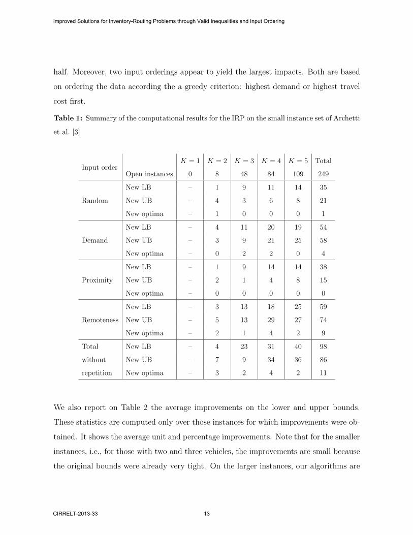
half. Moreover, two input orderings appear to yield the largest impacts. Both are based

on ordering the data according the a greedy criterion: highest demand or highest travel

cost first.

Table 1: Summary of the computational results for the IRP on the small instance set of Archetti

et al. [3]

Input orderK = 1 K = 2 K = 3 K = 4 K = 5 Total

Open instances 0 8 48 84 109 249

Random

New LB – 1 9 11 14 35

New UB – 4 3 6 8 21

New optima – 1 0 0 0 1

Demand

New LB – 4 11 20 19 54

New UB – 3 9 21 25 58


Proximity

New LB – 1 9 14 14 38

New UB – 2 1 4 8 15


Remoteness

New LB – 3 13 18 25 59

New UB – 5 13 29 27 74


Total New LB – 4 23 31 40 98

without New UB – 7 9 34 36 86

repetition New optima – 3 2 4 2 11

We also report on Table 2 the average improvements on the lower and upper bounds.

These statistics are computed only over those instances for which improvements were ob-

tained. It shows the average unit and percentage improvements. Note that for the smaller

instances, i.e., for those with two and three vehicles, the improvements are small because

the original bounds were already very tight. On the larger instances, our algorithms are


CIRRELT-2013-33 13

able to obtain average solution values which can be up to 50% better. In particular, for

each input ordering we show the average unit improvement on the bounds, followed by

the percentage improvement in parenthesis.

Table 2: Average improvements on the bounds for the open instances of the IRP on the small

instance set of Archetti et al. [3]

Input order in units (in %) K = 2 K = 3 K = 4 K = 5 Average

RandomAvg LB increase 74.83 (0.72) 56.83 (0.77) 173.83 (1.12) 108.72 (1.27) 103.55 (0.97)

Avg UB decrease 48.84 (0.58) 212.25 (2.49) 9120.72 (53.29) 4668.20 (28.01) 3512.50 (21.09)

DemandAvg LB increase 100.88 (0.90) 80.97 (0.81) 226.91 (2.12) 235.11 (2.62) 160.96 (1.61)

Avg UB decrease 14.34 (0.16) 163.31 (1.92) 5241.54 (34.41) 3443.33 (20.00) 2215.65 (14.12)

ProximityAvg LB increase 156.68 (1.44) 134.00 (0.69) 261.14 (1.78) 127.85 (0.98) 169.91 (1.22)

Avg UB decrease 1.90 (0.02) 159.43 (1.60) 7300.06 (44.53) 4636.07 (27.65) 3024.36 (18.45)

RemotenessAvg LB increase 90.92 (0.81) 147.24 (1.15) 200.19 (1.91) 219.83 (2.18) 164.54 (1.51)

Avg UB decrease 10.99 (0.11) 89.25 (0.91) 5819.62 (37.83) 2653.50 (15.31) 2143.34 (13.54)

TotalAvg LB increase 105.82 (0.96) 104.76 (0.85) 215.51 (1.73) 172.87 (1.76) 149.74 (1.32)

Avg UB decrease 19.01 (0.21) 156.06 (1.73) 6870.48 (42.51) 3850.27 (22.74) 2723.96 (16.80)

We have also applied our algorithm to the newer and larger testbed proposed in [4], which

contains 60 instances with six time periods and up to 200 customers. There are 20 in-

stances with 50 customers, 20 instances with 100 customers, and 20 instances with 200

customers. A time limit of four hours was imposed on the solution of each instance, only

one sixth of the time allowed by Coelho and Laporte [7]. We have succeeded in solving all

instances optimally for the single vehicle case. For all the 20 instances containing 50 cus-

tomers and with two vehicles we have obtained significant improvements. We do not report

solutions for larger instances because we have observed that the branch-and-cut algorithm

alone is rarely capable of finding a feasible solution within the allotted time. Detailed re-

sults on all instances are available for download from http://www.leandro-coelho.com/.

Finally we report on Table 4 the average unit and percentage improvements of the lower

and upper bounds for the instances where improvements were observed. Note again that


14 CIRRELT-2013-33

Table 3: Summary of the computational results for the IRP on the large instance set of Archetti

et al. [4]

Input orderK = 1 K = 2 Total

Open instances 43 20 63

Random

New LB 14 10 24

New UB 10 2 12

New optima 3 0 3

Demand

New LB 12 9 21

New UB 11 2 13

New optima 3 0 3

Proximity

New LB 14 7 21

New UB 9 2 11

New optima 3 0 3

Remoteness

New LB 10 9 19

New UB 8 4 12

New optima 3 0 3

Total New LB 18 14 32

without New UB 14 6 20

repetition New optima 3 0 3


CIRRELT-2013-33 15

the best improvements in the lower bounds were obtained by ordering the input from high

to low with respect to a given criterion, in this case the demand and the travel cost to

the supplier.

Table 4: Average improvements on the bounds for the open instances of the IRP on the large

instance set of Archetti et al. [3]

Input order in units (in %) K = 1 K = 2 Average

RandomAvg LB increase 46.08 (0.35) 59.80 (0.18) 52.94 (0.26)

Avg UB decrease 310.59 (1.63) 124.23 (0.75) 217.41 (1.19)

DemandAvg LB increase 43.58 (0.27) 84.95 (0.28) 64.26 (0.27)

Avg UB decrease 437.01 (2.04) 191.46 (1.25) 314.23 (1.64)

ProximityAvg LB increase 46.82 (0.30) 60.65 (0.20) 53.73 (0.25)

Avg UB decrease 322.27 (1.46) 212.50 (1.24) 267.38 (1.35)

RemotenessAvg LB increase 46.92 (0.35) 76.02 (0.30) 61.47 (0.32)

Avg UB decrease 380.92 (2.01) 150.30 (0.80) 265.61 (1.40)

TotalAvg LB increase 45.85 (0.31) 70.35 (0.24) 58.10 (0.27)

Avg UB decrease 362.69 (1.78) 169.62 (1.01) 266.15 (1.39)

6 Conclusions

We have developed new valid inequalities which hold for several classes of IRPs, and we

have tested the effect of changing the order of the input data on the quality of the bounds

obtained and on the running time. We have generated new best known solutions for

several large instances of the multi-vehicle IRP. We have also obtained improved lower

bounds for several instances when compared to previous best known solutions, besides

identifying new optimal solutions. We have increased the size of instances which we are

now capable of solving exactly within short computational times.


16 CIRRELT-2013-33

Acknowledgments

We thank Guy Desaulniers for his comments on a previous version of this paper. This work was

partly supported by the Canadian Natural Sciences and Engineering Research Council under

grant 39682-10. This support is gratefully acknowledged. We also thank Calcul Quebec for

providing computing facilities.

References

[1] Y. Adulyasak, J.-F. Cordeau, and R. Jans. Formulations and branch-and-cut algorithms

for multi-vehicle production and inventory routing problems. INFORMS Journal on Com-

puting, forthcoming, 2013.

[2] H. Andersson, A. Hoff, M. Christiansen, G. Hasle, and A. Løkketangen. Industrial as-

pects and literature survey: Combined inventory management and routing. Computers &

Operations Research, 37(9):1515–1536, 2010.

[3] C. Archetti, L. Bertazzi, G. Laporte, and M. G. Speranza. A branch-and-cut algorithm

for a vendor-managed inventory-routing problem. Transportation Science, 41(3):382–391,

2007.

[4] C. Archetti, L. Bertazzi, A. Hertz, and M. G. Speranza. A hybrid heuristic for an inventory

routing problem. INFORMS Journal on Computing, 24(1):101–116, 2012.

[5] W. J. Bell, L. M. Dalberto, M. L. Fisher, A. J. Greenfield, R. Jaikumar, P. Kedia, R. G.

Mack, and P. J. Prutzman. Improving the distribution of industrial gases with an on-line

computerized routing and scheduling optimizer. Interfaces, 13(6):4–23, 1983.

[6] L. E. Cardenas-Barron, J.-T. Teng, G. Trevino-Garza, H.-M. Wee, and K.-R. Lou. An

improved algorithm and solution on an integrated production-inventory model in a three-

layer supply chain. International Journal of Production Economics, 136(2):384–388, 2012.


CIRRELT-2013-33 17

[7] L. C. Coelho and G. Laporte. The exact solution of several classes of inventory-routing

problems. Computers & Operations Research, 40(2):558–565, 2013.

[8] L. C. Coelho and G. Laporte. A branch-and-cut algorithm for the multi-product multi-

vehicle inventory-routing problem. International Journal of Production Research, forth-

coming, 2013. doi: 10.1080/00207543.2012.757668.

[9] L. C. Coelho, J.-F. Cordeau, and G. Laporte. The inventory-routing problem with trans-

shipment. Computers & Operations Research, 39(11):2537–2548, 2012.

[10] L. C. Coelho, J.-F. Cordeau, and G. Laporte. Consistency in multi-vehicle inventory-

routing. Transportation Research Part C: Emerging Technologies, 24(1):270–287, 2012.

[11] L. C. Coelho, J.-F. Cordeau, and G. Laporte. Thirty years of inventory-routing. Trans-

portation Science, forthcoming, 2013.

[12] S. E. Elmaghraby. The economic lot scheduling problem (ELSP): review and extensions.

Management Science, 24(6):587–598, 1978.

[13] M. Gendreau, G. Laporte, and F. Semet. The covering tour problem. Operations Research,

45(4):568–576, 1997.

[14] Q. Gou, L. Liang, Z. Huang, and C. Xu. A joint inventory model for an open-loop reverse

supply chain. International Journal of Production Economics, 116(1):28–42, 2008.

[15] F. W. Harris. How many parts to make at once. Factory, The Magazine of Management,

10(2):135–136, 1913.

[16] R. Jans and J. Desrosiers. Binary clustering problems: Symmetric, asymmetric and decom-

position formulations. Technical Report G-2010-44, GERAD, Montreal, Canada, 2010.

[17] R. Jans and J. Desrosiers. Efficient symmetry breaking formulations for the job grouping

problem. Computers & Operations Research, 40(4):1132–1142, 2013.

[18] W. Klibi and A. Martel. Modeling approaches for the design of resilient supply networks

under disruptions. International Journal of Production Economics, 135(2):882–898, 2012.


18 CIRRELT-2013-33

[19] G. Laporte. Fifty years of vehicle routing. Transportation Science, 43(4):408–416, 2009.

[20] M. W. Padberg and G. Rinaldi. A branch-and-cut algorithm for the resolution of large-scale

symmetric traveling salesman problems. SIAM Review, 33(1):60–100, 1991.

[21] J. Rogers. A computational approach to the economic lot scheduling problem. Management

Science, 4(3):264–291, 1958.

[22] E. A. Silver and H. C. Meal. A heuristic for selecting lot size quantities for the case of

a deterministic time-varying demand rate and discrete opportunities for replenishment.

Production and Inventory Management, 14(2):64–74, 1973.

[23] S. A. Tarim and B. G. Kingsman. The stochastic dynamic production/inventory lot-sizing

problem with service-level constraints. International Journal of Production Economics, 88

(1):105–119, 2004.

[24] K. H. van Donselaar and R. A. C. M. Broekmeulen. Determination of safety stocks in a

lost sales inventory system with periodic review, positive lead-time, lot-sizing and a target

fill rate. International Journal of Production Economics, forthcoming, 2013.

[25] H. M. Wagner and T. M. Whitin. Dynamic version of the economic lot size model. Man-

agement Science, 5(1):89–96, 1958.


CIRRELT-2013-33 19

Improved Solutions for Inventory- Routing Problems through ... · Routing Problems through Valid...

Documents

Transcript of Improved Solutions for Inventory- Routing Problems through ... · Routing Problems through Valid...