Improved long-term thermal comfort indices for continuous ...

Preprint version. For published version go to https://doi.org/10.1016/j.enbuild.2020.110270

Improved long-term thermal comfort indices for continuous monitoring

Peixian Li a, b, *, Thomas Parkinson c, Stefano Schiavon c, Thomas M. Froese d, **, Richard de Dear e, Adam Rysanek f, Sheryl Staub-French b a Department of Building Engineering, College of Civil Engineering, Tongji University, Shanghai, China

b Department of Civil Engineering, University of British Columbia, Canada

c Center for the Built Environment, University of California, Berkeley, United States

d Department of Civil Engineering, University of Victoria, Canada

e School of Architecture, Design and Planning, University of Sydney, Australia

f School of Architecture and Landscape Architecture, University of British Columbia, Canada

* Corresponding author: Department of Building Engineering, College of Civil Engineering, Tongji University, 1239 Siping Road, Shanghai 200092, China. Email: [email protected]

** Corresponding Author: University of Victoria, Department of Civil Engineering, Engineering and Computer Science (ECS) 304, PO Box 1700 STN CSC, Victoria, BC, Canada V8W 2Y2. Email: [email protected], Tel: (1) 250-721-7066

Abstract

Thermal comfort standards have suggested a number of physical indices which can be calculated from either building simulations or in situ physical monitoring to assess the long-term thermal comfort of a space. However, the prohibitively high cost of sensor technologies has limited the applications of these physical indices, and their usefulness has never been established using data collected in real buildings. This paper is the first assessment of the six types of existing indices (23 total) found in standards and five types of new indices (36 total) and their correlation with the long-term thermal satisfaction of building occupants. Correlation analyses were based on continuous thermal comfort measurements and post-occupancy evaluation surveys from four air-conditioned office buildings in Sydney, Australia. We found that the majority of existing indices, especially those based on predicted mean vote (PMV) and predicted percentage dissatisfied (PPD) metrics, have a weak correlation with thermal satisfaction. The percentage of time outside a temperature range was the best-performing index from the standards ( ). A new index based on the percentage of − .63r = 0 time that daily temperature range is greater than a threshold reported the strongest correlation ( ) with thermal satisfaction for this dataset. The results suggest that − .8r = 0 occupants’ long-term thermal comfort is influenced more by pronounced excursions beyond some acceptable temperature range and large variations in daily temperature than the average experience over time. These findings support the use of continuous monitoring technologies for long-term thermal comfort evaluation and inform potential amendments of international thermal comfort standards.

Key words

Energy and Buildings, October 2020 Volume 224 1 https://doi.org/10.1016/j.enbuild.2020.110270

https://escholarship.org/uc/item/9h55w20w

mailto:[email protected]

mailto:[email protected]

https://doi.org/10.1016/j.enbuild.2020.110270




Thermal comfort, Building performance, Continuous monitoring, Post occupancy evaluation (POE), Workplace satisfaction, Data driven methods

Nomenclature

= air temperatureT a

= operative temperatureT o

= mean radiant temperatureT r

= globe temperatureT g

RH = relative humidity

PMV = predicted mean vote

PPD = predicted percentage dissatisfied.

Graphical abstract

1 Introduction

It is an oft-cited statistic that Americans spend up to 90% of their time indoors [1], with building occupants in many other countries having similar exposure to indoor environments. This notion that we are an indoor species is increasingly relevant in light of the mounting evidence that Indoor Environmental Quality (IEQ) significantly impacts occupants’ health, well-being and productivity [2]. As one of the main components of IEQ, thermal comfort is known to be a key determinant in the overall evaluation of indoor environments. While its ranked importance relative to other IEQ factors is debated, it is usually considered as one of the most important [3]. Yet 40% of occupants in US office buildings are dissatisfied with their thermal environment [4]. Thermal comfort has been shown to be a basic requirement for occupants, meaning it contributes overwhelmingly towards dissatisfaction but little towards positive evaluations when it is satisfactory [5]. Thermal comfort is also known to interact with







other IEQ factors such as indoor air quality [6,7]. It is clear, then, that efforts to improve IEQ and increase overall satisfaction should carefully consider the thermal comfort of building occupants.

The importance of thermal comfort to overall satisfaction with indoor environments is particularly relevant in commercial office buildings, where building managers are motivated to minimise any disruption or distraction resulting from thermal discomfort in the interest of employee productivity. A conventional practice is to tightly control the indoor environment within a range of conditions predicted to satisfy the majority of people. This is the approach adopted in thermal comfort standards such as ASHRAE 55 [8], ISO 7730 [9], and EN 16798 [10], which all specify different temperature ranges or Predicted Mean Vote (PMV) ranges as design guidelines for different building types and seasons.

Along with guidelines for the physical environment, assessing thermal comfort over time in existing buildings also requires subjective evaluations by occupants. Post-Occupancy Evaluation (POE) is a general approach of obtaining feedback about a building’s performance once it is built [11–17]. In commercial office buildings, it is common practice to assess the long-term satisfaction of occupants using POE surveys (e.g. BUS survey [18], CBE survey [19], BOSSA survey [20], etc.). Although these surveys are conducted at a point of time, their questions are often general and applicable for longer term insights (three to six months or more [8]). When combined with continuous IEQ data, these POE responses can be used to calculate long-term comfort indices designed to assess a thermal environment over time. Because of the prohibitive cost of installing and maintaining environmental sensors for continuous monitoring, previous application of long-term comfort indices has been limited to design phase assessments using data from building performance simulations. This led the majority of long-term comfort indices recommended by standards to be grafted with popular thermal comfort models such as PMV in order to increase their robustness and usefulness. While PMV [21] continues to be the dominant model used for thermal comfort assessments, researchers have reported inaccuracies of PMV model in predicting people’s thermal sensation in real buildings [22,23]. Besides the indices found in standards, other methods [24] suitable for design phase have been proposed such as the ExeedanceM index [25] and three indices to assess summer overheating risk [26–28]. Surprisingly, existing long-term indices from the standards have never been validated against long-term physical monitoring data in actual buildings nor against occupant feedback.

The recent proliferation of low-cost sensors for building IEQ measurements [29] and the rise of smart buildings have dissolved the barriers to assessing building performance with in situ long-term monitoring during the operational phase. These new sensor technologies have coincided with increasing awareness of the importance of long-term physical monitoring of built environments. Version 2 of the WELL Building Standard [30] now requires HVAC systems to both monitor and control air temperature, mean radiant temperature, relative humidity, and air speed in all regularly occupied spaces for the purposes of performance reporting and verification. A similar emphasis on sensors can be seen in the new RESET building performance standard [31] designed to certify buildings using continuous IEQ data gathered over three







months. These new standards highlight the growing interest in long-term indoor environmental monitoring for understanding and evaluating building performance.

There is a clear need to investigate the accuracy of the indices from standards in evaluating long-term thermal comfort in commercial office buildings. Do they reliably predict long-term subjective evaluations of thermal environments? If so, which index most closely corresponds with occupants’ actual levels of satisfaction? If not, are there better indices to evaluate long-term thermal comfort? The principal aim of this paper is to evaluate the predictive skill of existing long-term thermal comfort indices from standards and to propose new indices based on continuous, in situ physical monitoring and subjective evaluations from four air-conditioned office buildings.

2 Methods

To address the aim of this study, we conducted secondary data analyses using the Building Occupants Survey System Australia (BOSSA) database [20] and the Sentient Ambient Monitoring of Buildings in Australia (SAMBA) IEQ measurement database [29], both of which were developed by the Indoor Environmental Quality Lab at The University of Sydney. Figure 1 outlines the overall methodology. The BOSSA survey is comprised of retrospective questions regarding occupant long-term thermal satisfaction, and SAMBA measures the relevant thermal parameters continuously over time. We used responses to the BOSSA surveys to estimate long-term thermal comfort. A variety of physical indices calculated from the SAMBA database were then compared to the subjective index of long-term thermal comfort using Pearson correlation analysis. The stronger the correlation is, the better the physical index predicts the true long-term thermal comfort. The following sections describe the databases and data analyses in detail.

Figure 1 Methodology Diagram. The 3D render is the SAMBA IEQ Monitoring device.

2.1 BOSSA survey database and subjective index

BOSSA is a POE survey tool designed to automate the process of collecting occupants’ subjective assessments of their indoor environment [20]. Respondents are asked to rate their satisfaction with core building elements and functions such as overall design, physical environments, building maintenance, etc. As of July 2019, 91 BOSSA survey campaigns have







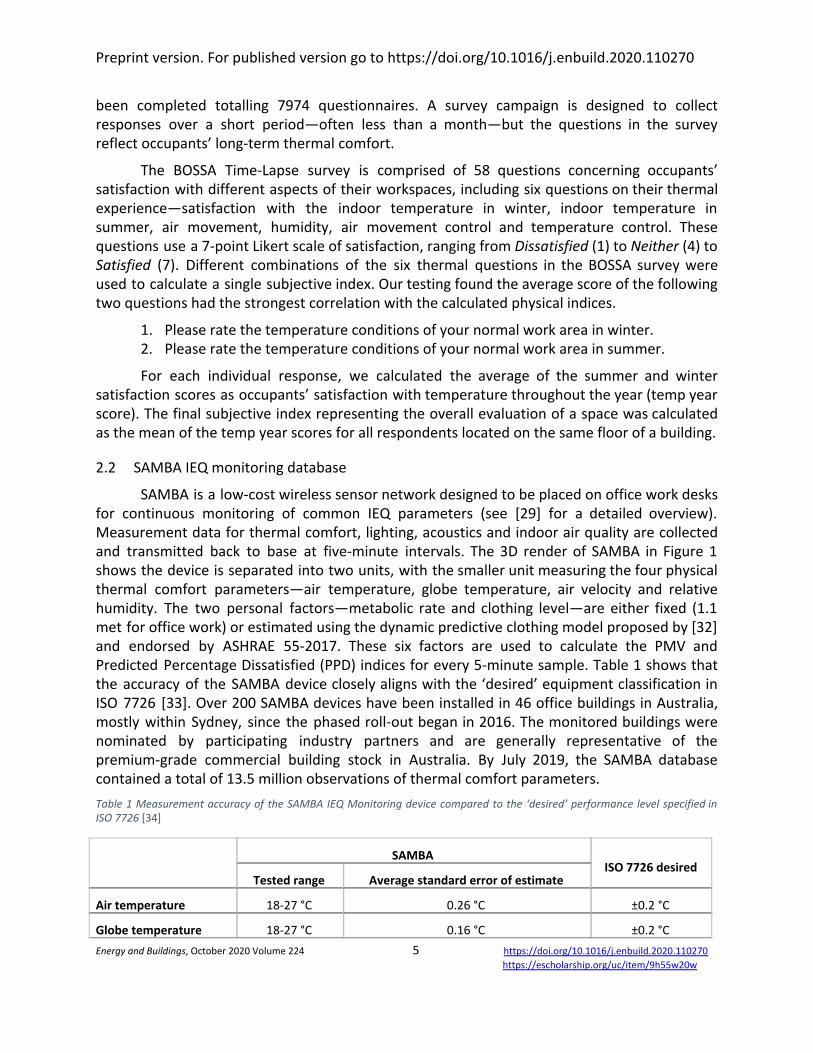
been completed totalling 7974 questionnaires. A survey campaign is designed to collect responses over a short period—often less than a month—but the questions in the survey reflect occupants’ long-term thermal comfort.

The BOSSA Time-Lapse survey is comprised of 58 questions concerning occupants’ satisfaction with different aspects of their workspaces, including six questions on their thermal experience—satisfaction with the indoor temperature in winter, indoor temperature in summer, air movement, humidity, air movement control and temperature control. These questions use a 7-point Likert scale of satisfaction, ranging from Dissatisfied (1) to Neither (4) to Satisfied (7). Different combinations of the six thermal questions in the BOSSA survey were used to calculate a single subjective index. Our testing found the average score of the following two questions had the strongest correlation with the calculated physical indices.

1. Please rate the temperature conditions of your normal work area in winter. 2. Please rate the temperature conditions of your normal work area in summer.

For each individual response, we calculated the average of the summer and winter satisfaction scores as occupants’ satisfaction with temperature throughout the year (temp year score). The final subjective index representing the overall evaluation of a space was calculated as the mean of the temp year scores for all respondents located on the same floor of a building.

2.2 SAMBA IEQ monitoring database

SAMBA is a low-cost wireless sensor network designed to be placed on office work desks for continuous monitoring of common IEQ parameters (see [29] for a detailed overview). Measurement data for thermal comfort, lighting, acoustics and indoor air quality are collected and transmitted back to base at five-minute intervals. The 3D render of SAMBA in Figure 1 shows the device is separated into two units, with the smaller unit measuring the four physical thermal comfort parameters—air temperature, globe temperature, air velocity and relative humidity. The two personal factors—metabolic rate and clothing level—are either fixed (1.1 met for office work) or estimated using the dynamic predictive clothing model proposed by [32] and endorsed by ASHRAE 55-2017. These six factors are used to calculate the PMV and Predicted Percentage Dissatisfied (PPD) indices for every 5-minute sample. Table 1 shows that the accuracy of the SAMBA device closely aligns with the ‘desired’ equipment classification in ISO 7726 [33]. Over 200 SAMBA devices have been installed in 46 office buildings in Australia, mostly within Sydney, since the phased roll-out began in 2016. The monitored buildings were nominated by participating industry partners and are generally representative of the premium-grade commercial building stock in Australia. By July 2019, the SAMBA database contained a total of 13.5 million observations of thermal comfort parameters.

Table 1 Measurement accuracy of the SAMBA IEQ Monitoring device compared to the ‘desired’ performance level specified in ISO 7726 [34]

SAMBA ISO 7726 desired

Tested range Average standard error of estimate

Air temperature 18-27 °C 0.26 °C ±0.2 °C

Globe temperature 18-27 °C 0.16 °C ±0.2 °C







Air speed 0.00-0.40 m/s 0.015 m/s ±0.02 m/s

Relative humidity 20-70% 1.04% ±2%

2.3 Data preparation

Records from both the BOSSA and SAMBA databases are time-stamped and spatially tagged to either a zone or a floor of a building to allow spatiotemporal pairing of subjective data with physical measurements. For this study, we matched responses from BOSSA campaigns to SAMBA measurements made on the same floor of the same building at close-to-or-during the time of the BOSSA survey campaign. We identified 33 pairings of BOSSA campaigns and SAMBA time series data (Table 2) in four office buildings in the central business district in Sydney, Australia. A total of 970 individual survey responses and 2.3 million physical measurements of thermal comfort parameters were used in our analysis. Table 2 summarizes the time of the BOSSA survey campaign, number of responses for each survey campaign, periods of physical monitoring, and the number of workdays (excluding weekends) of monitoring. Four survey campaigns on level 28 in building D had less than ten responses, and subsequent analyses were designed to address the statistical significance from such low numbers. This will be discussed further in the results section.

Comfort standards do not give clear guidelines to determine the minimum or ideal range of continuous measurements for this type of analysis. Long-term assessment criteria found in ISO 7730, EN 16798 and ASHRAE 55 simply state that the monitoring period should be representative of the conditions overall. To best address this, we prioritised instances where there was an entire year of SAMBA data (i.e. Building D) because the total variance in the thermal environment can be captured over the typical annual certification period used by most rating systems. For buildings without a full year of measurements, we used any available SAMBA data beginning or ending within one month of a BOSSA campaign (i.e. Building A, B, and C).

After data preparation, there was one year of measurements for Building A and D, 87 workdays for Building B, and 108 workdays for Building C. We wondered if the shorter monitoring periods in Building B and C would sufficiently characterize the long-term conditions experienced by the occupants, and whether IEQ measurements collected after the BOSSA campaign are useful given that the long-term satisfaction questions are retrospective. Visual inspection of the SAMBA data from the building zones showed relatively stable conditions throughout the monitoring period. Comparing air temperature before and after the survey campaigns in the 10 pairs of datasets where the BOSSA campaigns overlapped the SAMBA measurements, the average difference in mean air temperature was 0.27 °C ± 0.26 °C (standard deviation). These small differences indicate that the shorter datasets available in Buildings B and C are sufficient for characterising the low temperature variance expected in premium-grade air-conditioned offices. They also suggest that retrospective survey responses are likely to be just as relevant to prospective physical measurements. We therefore included these datasets in our analysis.







Table 2 Matched BOSSA survey campaigns and SAMBA measurements included in our analyses

Building Floor No. of survey responses

BOSSA start BOSSA end SAMBA start SAMBA end Workdays of SAMBA

A Level 19 20 2017-03-23 2017-03-30 2017-04-03 2019-03-15 270

B Level 10 107 2018-04-20 2018-05-18 2018-07-16 2018-12-12 87

B Level 9 74 2018-04-20 2018-05-17 2018-07-16 2018-12-06 86

C Level 12 19 2018-02-22 2018-03-07 2018-01-26 2019-05-14 302

C Level 2 31 2018-09-26 2018-10-08 2018-06-29 2019-04-29 217

C Level 21 48 2016-11-21 2016-12-01 2017-02-01 2018-02-01 262

C Level 21 45 2017-06-09 2017-06-22 2017-02-01 2018-02-01 262

C Level 6 39 2016-11-21 2016-11-30 2016-09-09 2017-05-17 108

C Level 6 44 2017-06-07 2017-11-27 2016-09-09 2017-05-17 108

D Level 25 20 2016-12-06 2016-12-15 2016-09-15 2017-09-29 261

D Level 25 11 2018-03-12 2018-03-14 2017-03-01 2018-03-20 186

D Level 25 14 2018-08-14 2018-09-06 2017-08-01 2018-09-10 180

D Level 25 18 2019-05-01 2019-05-08 2018-05-17 2019-07-02 287

D Level 26 19 2016-12-06 2016-12-19 2016-09-15 2017-09-29 266

D Level 26 15 2018-03-12 2018-03-15 2017-03-01 2018-03-20 275

D Level 26 21 2018-08-14 2018-08-22 2017-08-01 2018-08-30 258

D Level 26 22 2019-05-01 2019-05-20 2018-05-01 2019-07-16 230

D Level 27 30 2016-12-06 2016-12-19 2016-10-11 2017-09-29 233

D Level 27 19 2018-03-12 2018-03-16 2017-03-01 2018-03-20 257

D Level 27 30 2018-08-14 2018-09-03 2017-08-01 2018-09-06 235

D Level 27 10 2019-05-01 2019-05-06 2018-05-01 2019-07-17 219

D Level 28 7 2016-12-06 2016-12-19 2016-10-10 2017-09-29 249

D Level 28 3 2018-03-12 2018-03-14 2017-03-01 2018-03-20 275

D Level 28 8 2018-08-14 2018-09-06 2017-08-01 2018-09-10 290

D Level 28 3 2019-05-01 2019-05-06 2018-05-01 2019-07-16 316

D Level 29 34 2016-12-06 2016-12-27 2016-10-10 2017-09-29 252

D Level 29 25 2018-03-12 2018-03-19 2017-03-01 2018-03-20 275

D Level 29 29 2018-08-14 2018-09-10 2017-08-01 2018-09-10 262

D Level 29 23 2019-05-01 2019-05-06 2018-05-01 2019-07-16 272

D Level 30 49 2016-12-02 2016-12-19 2016-08-09 2017-09-29 298

D Level 30 40 2018-03-04 2018-03-19 2017-03-01 2018-03-20 275

D Level 30 46 2018-08-14 2018-08-27 2017-08-01 2018-09-10 289

D Level 30 47 2019-05-01 2019-05-27 2018-05-01 2019-07-16 315







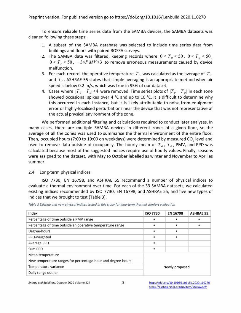
To ensure reliable time series data from the SAMBA devices, the SAMBA datasets was cleaned following these steps:

1. A subset of the SAMBA database was selected to include time series data from buildings and floors with paired BOSSA surveys.

2. The SAMBA data was filtered, keeping records where , , 00 < T a < 5 00 < T g < 5 , to remove erroneous measurements caused by device00 < T r < 5 ≤PMV ≤3− 3

malfunction. 3. For each record, the operative temperature was calculated as the average of T o T a

and . ASHRAE 55 states that simple averaging is an appropriate method when air T r speed is below 0.2 m/s, which was true in 95% of our dataset.

4. Cases where were removed. Time series plots of in each zone 4T| o − T a| ≥ T || o − T a showed occasional spikes over 4 °C and up to 10 °C. It is difficult to determine why this occurred in each instance, but it is likely attributable to noise from equipment error or highly-localised perturbations near the device that was not representative of the actual physical environment of the zone.

We performed additional filtering and calculations required to conduct later analyses. In many cases, there are multiple SAMBA devices in different zones of a given floor, so the average of all the zones was used to summarise the thermal environment of the entire floor. Then, occupied hours (7:00 to 19:00 on weekdays) were determined by measured CO2 level and used to remove data outside of occupancy. The hourly mean of , , PMV, and PPD was T a T o calculated because most of the suggested indices require use of hourly values. Finally, seasons were assigned to the dataset, with May to October labelled as winter and November to April as summer.

2.4 Long-term physical indices

ISO 7730, EN 16798, and ASHRAE 55 recommend a number of physical indices to evaluate a thermal environment over time. For each of the 33 SAMBA datasets, we calculated existing indices recommended by ISO 7730, EN 16798, and ASHRAE 55, and five new types of indices that we brought to test (Table 3).

Table 3 Existing and new physical indices tested in this study for long-term thermal comfort evaluation

Index ISO 7730 EN 16798 ASHRAE 55

Percentage of time outside a PMV range • • •

Percentage of time outside an operative temperature range • • •

Degree-hours • •

PPD-weighted • •

Average PPD •

Sum PPD •

Mean temperature

Newly proposed

New temperature ranges for percentage-hour and degree-hours

Temperature variance

Daily range outlier







Combined index

2.4.1 Existing long-term physical indices

The six existing types of indices recommended by comfort standards contain a total of 23 individual physical indices. The calculation methods for them are given in Equations 1 – 10.

1) Percentage of time outside a PMV range

ndex ×100#i = total number of occupied hoursnumber of hours that PMV >limit | | (1)

ISO 7730 and EN 16798 prescribe three PMV classes (Table 4), leading to three indices in this type: , , and .|PMV | .2% > 0 |PMV | .5% > 0 |PMV | .7% > 0

Table 4 Comfort classifications based on PMV ranges and corresponding PPD levels prescribed in ISO 7730 and EN 16798

PMV range PPD (%) ISO 7730 class A, EN 16798 class I –0.2 < PMV< +0.2 <6 ISO 7730 class B, EN 16798 class II –0.5 < PMV< +0.5 <10 ISO 7730 class C, EN 16798 class III –0.7 < PMV< +0.7 <15

2) Percentage of time outside a specified operative temperature range

ndex ×100#i = total number of occupied hoursnumber of hours that T outside the range o (2)

ISO 7730 and EN 16798 recommend operative temperature ranges for different building types (i.e. different activities) and seasons (i.e. different clothing level). Table 5 shows the operative temperature ranges recommended for offices, and thus there are six indices corresponding to six temperature ranges.

Table 5 Comfort classifications based on operative temperature ranges for summer and winter in office buildings in European standards

Summer (°C) Winter (°C) ISO 7730 class A 23.5 – 25.5, 4.5T o.optimal = 2 21 – 23, 2T o.optimal = 2

ISO 7730 class B 23 – 26, 4.5T o.optimal = 2 20 – 24, 2T o.optimal = 2

ISO 7730 class C 22 – 27, 4.5T o.optimal = 2 19 – 25, 2T o.optimal = 2

EN 16798 class I <= 25.5 >= 21 EN 16798 class II <= 26 >= 20 EN 16798 class III <= 27 >= 19

3) Degree-hours

The degree-hours index is calculated as the product sum of the weighting factors and exposure time (Eq 5). The weighting factor for each hour is associated with the exceedance magnitude of operative temperature beyond the specified range. The weighting factor is calculated differently in ISO 7730 (Eq 3) and EN 16798 (Eq 4). This type includes six indices corresponding to the six different ranges in Table 5.







1 , T or T 0, T #wf ISO = { + T −T| o o.limit|T −T| o.optimal o.limit| o ≥ T o.limit.upper o ≤ T o.limit.lower o.limit.lower < T o < T o.limit.upper (3)

|T |, T or T 0, T #wfEN = { o − T o.limit o > T o.limit.upper o < T o.limit.lower o.limit.lower ≤ T o ≤ T o.limit.upper (4)

ndex f ·t#i = ∑

w (5)

4) PPD-weighted

The hours during which PMV exceeds the range are summed and weighted by a factor determined by PPD. The calculation of weighting factors is different between ISO 7730 (Eq 6) and EN 16798 (Eq 7) but the formula for the PPD-weighted index is identical (Eq 8)—product sum of the weighting factors through time. There are three PMV classes and two calculation formulae resulting in six indices for this type.

, |PMV |≥|PMV | 0, PMV | #wf ISO = { PPDPMV .limit

PPDPMV .actual actual limit PMV|| actual

|| < | limit (6)

, |PMV | PMV | 0, |PMV | #wfEN = { PPDPMV .limit

PPDPMV .actual actual > | limit PMV|| actual

|| ≤ limit (7)

ndex f ·t#i = ∑

w (8)

is the PPD corresponding to the actual PMV. is the PPDPPDPMV .actual PPDPMV .limit corresponding to as listed in Table 4.PMV limit

5) Average PPD

ndex #i =PD∑

P

total number of occupied hours (9)

6) Sum PPD

ndex PD#i = ∑

P (10)

The different time series lengths of the 33 SAMBA datasets effects the calculation of the time-dependent indices i.e. degree-hours, PPD-weighted, and Sum PPD. To address this, we normalized those indices by dividing them by the total number of hours measured.

2.4.2 New long-term physical indices

We tested a variety of new physical indices based on different IEQ parameters, many of which were not correlated with long-term comfort survey responses, i.e. those based on air speed and humidity. This section describes new physical indices that showed correlation with subjective evaluation to some degree. Existing indices found in standards use operative temperature as an input, but air temperature is more readily available in almost any building. For this reason, we decided to test the performance of the new indices using both operative and air temperature. The calculation of the new indices are as follows.

1) Mean temperature







This type of indices uses the mean and mean of each SAMBA dataset.T a T o

ndex #i = or ∑

T a ∑

T o

total number of occupied hours (11)

2) New temperature ranges

In this category, percentage-hour and degree-hour indices are calculated using Eq 2, Eq 4 and Eq 5 but with different temperature ranges to those defined in ISO 7730 and EN 16798. The new temperature ranges for and are derived using percentiles, mean, and standard T a T o deviation of the SAMBA time series data. A total of 20 indices of this type were tested and are summarised in Table 6.

Table 6 Temperature ranges derived from time series data that were used in the calculation of the new comfort indices. Four are based on percentiles and one on standard deviation, with different temperature ranges specified for summer and winter seasons. Measured temperatures were quite stable in the monitored offices so the derived temperature ranges are similar.

Operative temperature °C Air temperature °C

Range name Meaning Summer Winter Summer Winter

P20 The 40th to 60th percentile 23.6 – 24.0 23.3 – 23.6 23.3 – 23.7 23.1 – 23.5




1sd Mean ± 1sd 22.9 – 25.0 22.7 – 24.2 22.6 – 24.8 22.5 – 24.2

3) Temperature variance

This index is based on the sample variance of the hourly average temperature for each SAMBA dataset and calculates the index as:

ndex or #i = n−1

∑n

i=1(T −T )a, i a

2

n−1

∑n

i=1(T −T )o,i o

2

(12)

where n = total number of occupied hours; and are the sample mean T a T o temperatures.

4) Daily range outlier

The range of temperatures measured over each business day is used to calculate the index as the percentage of days where that range exceeds a nominal threshold.

ndex ×100#i = total number of occupied daysnumber of days that T or T daily range>a threshold a o (13)

For this analysis, we set the threshold based on percentiles of the observed daily ranges in the SAMBA time series data. Ten different values were tested (Table 7) to determine the threshold with the strongest correlation to thermal satisfaction. Weekly ranges were tested but reported weaker correlations than daily variance and were therefore dropped from the analysis.







Table 7 Percentile thresholds tested for the daily range outlier indices. Stable conditions in the monitored offices results in a daily variance of less than 2.5°C in most cases

Percentile 50th 60th 70th 80th 90th daily range (°C) T a 1.31 1.48 1.69 2.00 2.48

daily range (°C) T o 1.20 1.36 1.56 1.83 2.29

5) Combined index

We combined the best-performing existing index and the best-performing new index in Eq 14. This normalised index from 0 to 100 considers if the absolute temperature is within an acceptable range and whether the daily variance in temperature exceeds the percentile threshold.

ndexi = ( total number of occupied hoursnumber of hours that T or T outside ISO B ranges a o + total number of occupied days

number of days that T or T daily range>the 80th pera o (14)

2.5 Correlation analysis

Pearson correlation analysis was used to investigate the linear relationship between the subjective index and physical indices. We chose to report the Pearson coefficient ( ) because it r is independent of the unit of measurement and is symmetric between X and Y, removing the need to scale the input data. There is no consensus on what is considered a strong linear relationship. Interpretation of the Pearson coefficient varies between fields and depends on the stated aims of the study. For clinicians, 0.2, 0.5, and 0.8 were suggested as the thresholds to differentiate weak, moderate, and strong associations [35]. For psychological analysis, even lower thresholds may be used i.e. 0.1, 0.2, and 0.3 [36]. In general statistics, threholds can be 0.3, 0.5, and 0.7 [37], or 0.1, 0.3, and 0.5 [38], or 0.3 and 0.5 [39]. Regardless of the differences between disciplines, a higher correlation coefficient is more desirable as it indicates a stronger relationship between the physical index and the subjective index. In this analysis, we use absolute coefficient values of 0.3, 0.5, and 0.7 (the 30th, 50th, and 90th percentiles of the resulted 59 coefficients) to indicate weak, moderate, and strong linear relationships respectively, and

as indicating statistical significance of the correlation..05p < 0

Given the small sample size (N = 33) we used 10-repeated-10-fold-cross-validated linear regressions for all correlation analyses to improve the robustness of the results. In 10-fold cross-validation, the original sample is randomly partitioned into ten equal size subsamples. Nine subsamples were used to train a linear regression model, and the remaining single subsample was the validation data for testing the model. This process was repeated ten times (the folds), with each of the ten subsamples used exactly once as the validation data. The 10-fold cross-validation was then repeated 10 times, generating 100 (10*10) training-and-testing subsamples for each of the physical indices. Mean Absolute Error (MAE), the average absolute difference between observed and predicted outcomes, measures the performance of the indices such that the lower the MAE, the better the index.

All analyses were performed using R Studio and R version 3.6.1 (2019-07-05) [40], along with the dplyr v0.8.3 [41], tidyr v0.8.3 [42], reshape2 v1.4.3 [43], lubridate v 1.7.4 [44], zoo v 1.8.6 [45], caret v6.0.84 [46], ggplot2 v3.2.0 [47], ggpubr v0.2.1 [48], and gridExtra v2.3 [49] packages.







3 Results

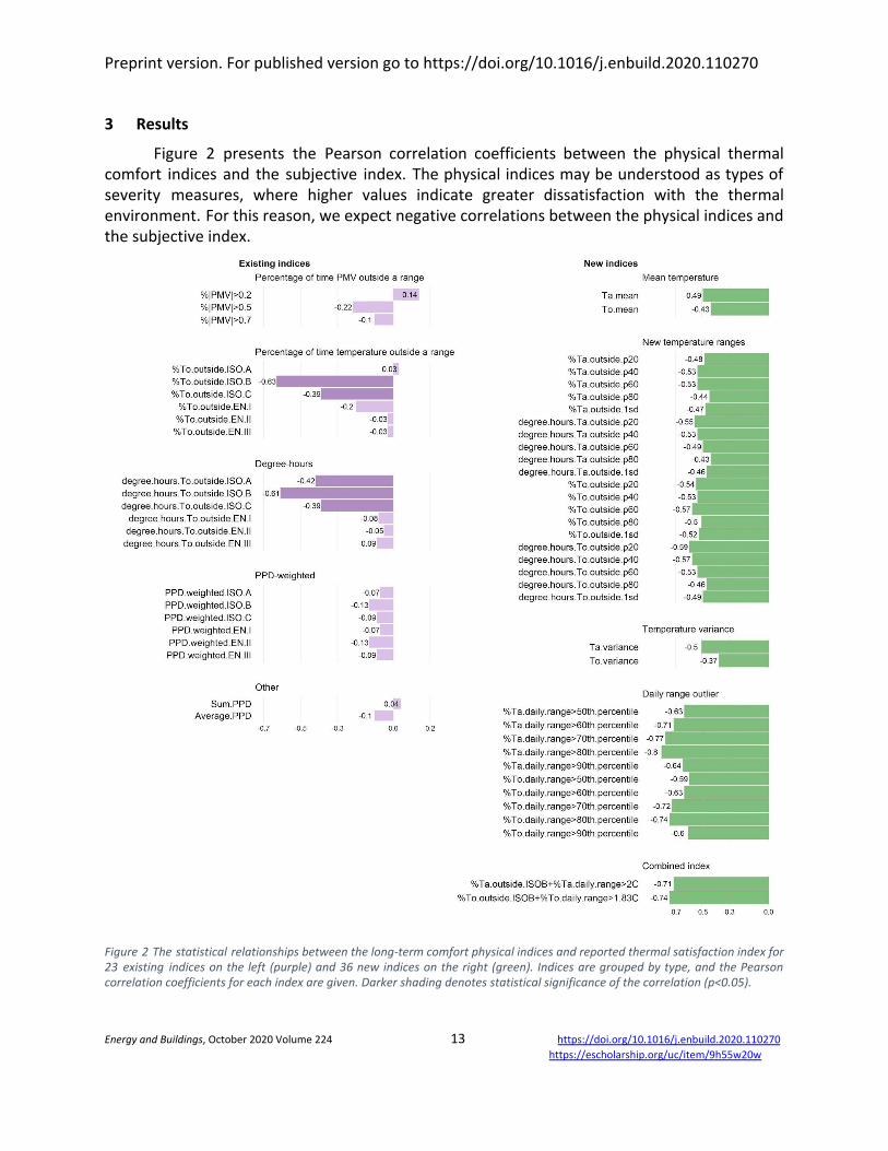
Figure 2 presents the Pearson correlation coefficients between the physical thermal comfort indices and the subjective index. The physical indices may be understood as types of severity measures, where higher values indicate greater dissatisfaction with the thermal environment. For this reason, we expect negative correlations between the physical indices and the subjective index.

Figure 2 The statistical relationships between the long-term comfort physical indices and reported thermal satisfaction index for 23 existing indices on the left (purple) and 36 new indices on the right (green). Indices are grouped by type, and the Pearson correlation coefficients for each index are given. Darker shading denotes statistical significance of the correlation (p<0.05).







Of the existing indices found in thermal comfort standards, only two—degree-hours T o outside ISO B and % outside ISO B—have a strong linear relationship with the subjective T o index. This indicates that the more times and the larger deviations that was outside a T o specified temperature range, the more occupants felt dissatisfied over time. Besides, physical indices based on PMV/PPD all reported weak linear relationships with thermal satisfaction. This may be due to the inaccuracies of steady-state heat balance models in non-uniform and dynamic environments.

The performance of the new indices shown in Figure 2 indicate that those based on mean temperatures, modified temperature ranges, and overall temperature variance have weak to moderate linear relationships with the subjective comfort measure. However, the daily range outlier indices show strong negative relationships to thermal satisfaction and out-perform most of the existing indices. The highest correlation coefficient is 0.8 for the daily air temperature variance above the 80th percentile (2 °C). In other words, increases in the daily occurrences of an air temperature range greater than 2 °C are highly correlated with lower occupant thermal satisfaction for this dataset.

Combining the better-performing existing index with the new range outlier index for both and resulted in slightly lower correlation coefficients than the range outlier indices T o T a alone. However, the combined indices still report strong linear relationship for both the operative ( and air temperature ) variants. The slight decrease in − .74) r = 0 r − .71( = 0 correlation strength in the air temperature index may be due to ISO class B ranges being specified for operative temperatures. Nevertheless, the new combined indices outperform any of the existing indices and have the advantage of defining a static temperature range modulated by a dynamic component.

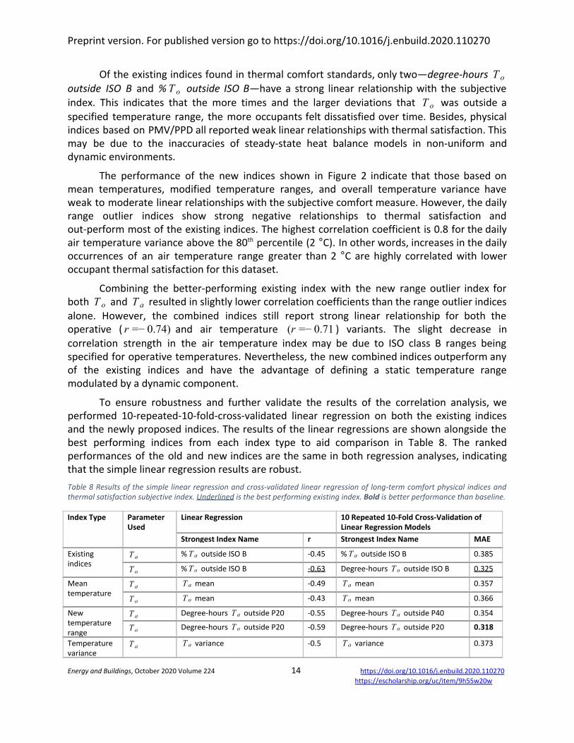
To ensure robustness and further validate the results of the correlation analysis, we performed 10-repeated-10-fold-cross-validated linear regression on both the existing indices and the newly proposed indices. The results of the linear regressions are shown alongside the best performing indices from each index type to aid comparison in Table 8. The ranked performances of the old and new indices are the same in both regression analyses, indicating that the simple linear regression results are robust.

Table 8 Results of the simple linear regression and cross-validated linear regression of long-term comfort physical indices and thermal satisfaction subjective index. Underlined is the best performing existing index. Bold is better performance than baseline.

Index Type Parameter Used

Linear Regression 10 Repeated 10-Fold Cross-Validation of Linear Regression Models

Strongest Index Name r Strongest Index Name MAE

Existing indices

T a % outside ISO BT a -0.45 % outside ISO BT a 0.385

T o % outside ISO BT o -0.63 Degree-hours outside ISO BT o 0.325

Mean temperature

T a meanT a -0.49 meanT a 0.357

T o meanT o -0.43 meanT o 0.366

New temperature range

T a Degree-hours outside P20T a -0.55 Degree-hours outside P40T a 0.354

T o Degree-hours outside P20T o -0.59 Degree-hours outside P20T o 0.318

Temperature variance

T a varianceT a -0.5 varianceT a 0.373







T o varianceT o -0.37 varianceT o 0.366

Daily range outlier

T a % daily range > 2 °CT a -0.80 % daily range > 2 °CT a 0.266

T o % daily range > 1.83 °CT o -0.74 % daily range > 1.83 °CT o 0.268

Combined index

T a % outside ISO B + % dailyT a T a

range > 2 °C

-0.71 % outside ISO B + % dailyT a T a

range > 2 °C

0.326

T o % outside ISO B + % dailyT o T o

range > 1.83 °C

-0.74 % outside ISO B + % dailyT o T o

range > 1.83 °C

0.286

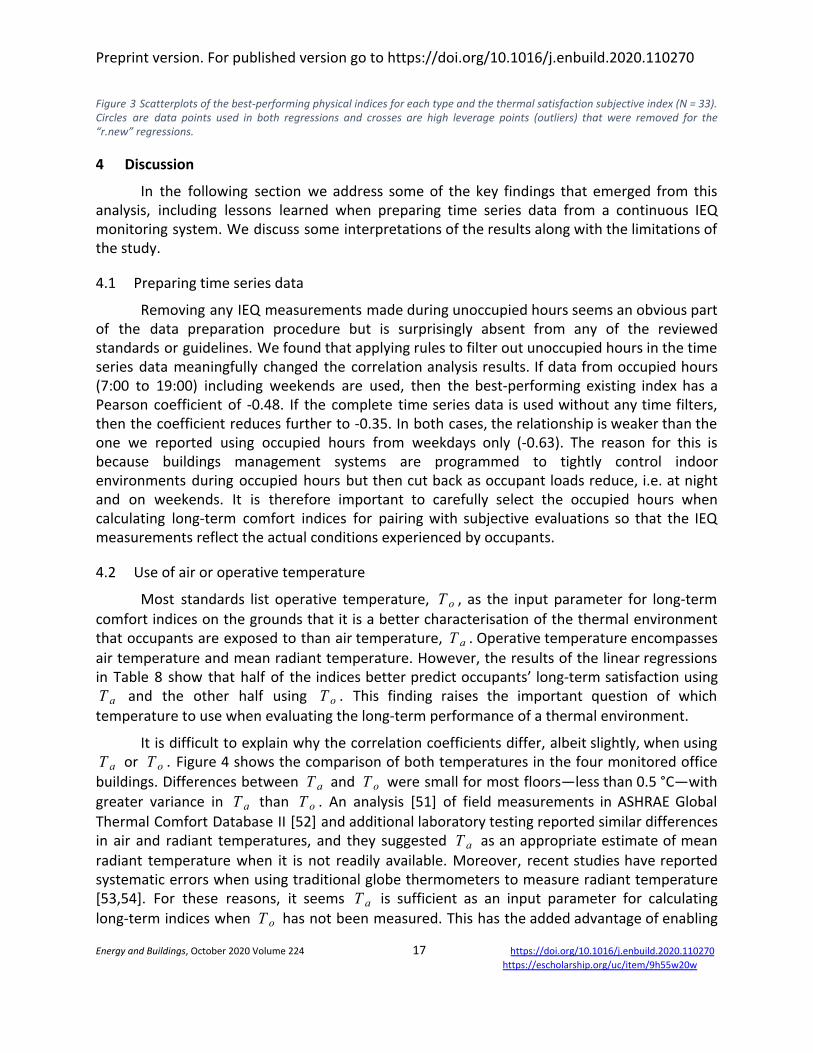
We investigated the effect of outliers on the results of the linear regression using the Cook’s distance test [50] to identify high leverage points. The Cook’s distance measures the change in regression models when each of the observations is removed. Higher values in the Cook’s distance indicate that removing a given observation will lead to a large change in the regression. When the Cook’s distance is greater than 4/N (N = 33 in our analysis), the observation is deemed a high leverage point, also known as an outlier. Figure 3 presents scatterplots for the 12 best performing indices from each index type listed in Table 8. Coefficients are inset for both the regression with all data points (r) and with outliers removed (r.new). As expected, removing high leverage points increased correlation strength in most cases. Though not marked in Figure 3, most outliers are from building D level 28 where the number of survey responses was small.







Figure 3 Scatterplots of the best-performing physical indices for each type and the thermal satisfaction subjective index (N = 33). Circles are data points used in both regressions and crosses are high leverage points (outliers) that were removed for the “r.new” regressions.

4 Discussion

In the following section we address some of the key findings that emerged from this analysis, including lessons learned when preparing time series data from a continuous IEQ monitoring system. We discuss some interpretations of the results along with the limitations of the study.

4.1 Preparing time series data

Removing any IEQ measurements made during unoccupied hours seems an obvious part of the data preparation procedure but is surprisingly absent from any of the reviewed standards or guidelines. We found that applying rules to filter out unoccupied hours in the time series data meaningfully changed the correlation analysis results. If data from occupied hours (7:00 to 19:00) including weekends are used, then the best-performing existing index has a Pearson coefficient of -0.48. If the complete time series data is used without any time filters, then the coefficient reduces further to -0.35. In both cases, the relationship is weaker than the one we reported using occupied hours from weekdays only (-0.63). The reason for this is because buildings management systems are programmed to tightly control indoor environments during occupied hours but then cut back as occupant loads reduce, i.e. at night and on weekends. It is therefore important to carefully select the occupied hours when calculating long-term comfort indices for pairing with subjective evaluations so that the IEQ measurements reflect the actual conditions experienced by occupants.

4.2 Use of air or operative temperature

Most standards list operative temperature, , as the input parameter for long-term T o comfort indices on the grounds that it is a better characterisation of the thermal environment that occupants are exposed to than air temperature, . Operative temperature encompasses T a air temperature and mean radiant temperature. However, the results of the linear regressions in Table 8 show that half of the indices better predict occupants’ long-term satisfaction using

and the other half using . This finding raises the important question of whichT a T o temperature to use when evaluating the long-term performance of a thermal environment.

It is difficult to explain why the correlation coefficients differ, albeit slightly, when using or . Figure 4 shows the comparison of both temperatures in the four monitored officeT a T o

buildings. Differences between and were small for most floors—less than 0.5 °C—with T a T o greater variance in than . An analysis [51] of field measurements in ASHRAE Global T a T o Thermal Comfort Database II [52] and additional laboratory testing reported similar differences in air and radiant temperatures, and they suggested as an appropriate estimate of mean T a radiant temperature when it is not readily available. Moreover, recent studies have reported systematic errors when using traditional globe thermometers to measure radiant temperature [53,54]. For these reasons, it seems is sufficient as an input parameter for calculating T a long-term indices when has not been measured. This has the added advantage of enabling T o







the use of continuous temperature records from building management systems for long-term evaluation of existing buildings.

Figure 4 Comparison of air temperature and operative temperature in the studied SAMBA datasets. Red dashed line is zero. The lower and upper hinges of the boxplots correspond to the 25th and 75th percentiles. The middle black bars are the medians.

4.3 Specifying index thresholds

We reported a higher correlation between the middle temperature range specified in ISO 7730 (ISO class B) and occupants’ thermal satisfaction compared to both the narrower (class A) and the wider range (class C). A similar pattern was observed for the new daily range outlier indices also, where the correlation with the 80th percentile was stronger than with the 70th or 90th percentiles. One possible explanation for this finding is that the index used to characterise the physical environment needs to have an appropriate level of sensitivity to distinguish periods when thermal conditions in an office are satisfactory from periods when it is unsatisfactory. If the temperature range or the threshold for the daily range outlier indices are too narrow, then the likelihood of a false negative classification is increased (i.e. conditions are measured to be outside the range or threshold even though occupants report satisfaction). Conversely, setting the boundaries too wide increases the likelihood of a false positive classification (i.e., conditions are measured to be within the range or threshold even though occupants report dissatisfaction).

Results from the monitored buildings in this study showed that ISO class B temperature range and a 2 °C threshold for daily range are the best indices to estimate occupant thermal T a







satisfaction. It is possible, however, that the most appropriate index range or thresholds may vary with occupancy type, floor layout, and/or building design. For this reason, we caution against prematurely prescribing those specific range or threshold values as design guidelines for all buildings. Doing so would encourage excessive HVAC energy use to maintain stable indoor conditions during building operation. Instead, careful attention should be given to correctly specifying the index thresholds to best align with the thermal expectations of occupants for a given building.

4.4 Occupant adaptation and sensitivity to variation

The results of the correlation analysis showed mean operative temperature has a moderate linear relationship with the subjective evaluation ( ), yet the frequency that − .43r = 0 operative temperature is outside a range is a better predictor of thermal (dis)satisfaction (

). Furthermore, absolute variation in operative temperature has a lower .63r = − 0 correlation with the long-term thermal satisfaction ( ) than the frequency with .37r = − 0 which daily temperature changes exceed a wide range ( ). These findings indicate the − .74r = 0 possibility of more extreme excursions beyond some acceptable temperature range holding greater influence over occupants’ long-term satisfaction than the average experience over time. Although the monitored buildings are centrally conditioned, the following section will explore the results within the framework of adaptive comfort theory. Doing so allows us to connect our findings to the idea that occupants’ thermal expectations and the availability of adaptive opportunities can shape long-term thermal satisfaction in a building.

One of the central tenets of adaptive comfort theory is that occupants actively respond to changing indoor environments by adjusting their behaviors and expectations [55]. The efficacy of those adjustments is influenced by a number of factors ranging from building type and design, workplace culture, and thermal physiology. Occupants are generally forgiving of moderate temperature variations because they are able to successfully regulate their personal environment to achieve thermal comfort. A common example is putting on a sweater when it is cool or initiating a desk fan when it is warm. However, instances in which the magnitude of the variation exceeds the adaptive ability of occupants is much more likely to lead to expressions of dissatisfaction. In such cases, the indoor environment did not meet the expectations of the occupant or their capacity to adapt.

The results suggested that more extreme deviations in comfort may dominate occupants’ long-term evaluation of the space. The evidence supporting this statement is the strong negative relationship reported between the frequency that varies greater than 2 °C T a in a day and the reported thermal satisfaction. Interestingly, this threshold is identical to field observations made by Humphreys in 1970s [56] who reported very similar findings. However, the four monitored buildings are premium-grade offices with HVAC systems designed to deliver a narrow temperature range. Measurements of air temperature reported in Table 6 and Table 7 show that there is little variation in normal daily conditions in these offices. The majority of BOSSA survey respondents (76%) had worked in their building for more than six months, so it is reasonable to assume that they had come to expect uniform temperatures considering the reported impact of thermal history on thermal expectations [57]. When unexpected deviations in those conditions occurred, those building occupants reported lower satisfaction. It is







possible, then, that the source of dissatisfaction is not with the variation in temperature from some absolute target range but rather with the fact that the indoor environment did not deliver the conditions that building occupants had come to expect.

The question emerging from the results of our study is whether dissatisfaction arises from variability in temperature per se, or if it is because occupants were not able to properly respond and adapt to conditions that did not meet their expectations. Simply concluding that occupants of these buildings prefer stable daily temperatures would contradict a large amount of extant literature on adaptation and variability. For example, a meta-analysis of ASHRAE Global Thermal Comfort Database II [58] showed that acceptable temperatures extend across a wide range of conditions, and vary depending on building type and climate/culture. And there is emerging evidence that building occupants adapt to the indoor temperatures they experience on a day-to-day basis irrespective of climate or building conditioning strategy [59]. These studies all highlight the importance of occupants’ expectations of a building in defining their comfort temperatures. Our results support this idea by showing that thermal satisfaction is less about the absolute indoor temperature than it is about exceeding some variability threshold. Or put another way, instances of dissatisfaction occur when the magnitude of variation exceeds the adaptive opportunities available to occupants. It may be that variability is only a problem when building occupants have come to expect constant, stable conditions that are afforded by modern HVAC systems. One practical solution would be to relax tight setpoint control and provide occupants with personal comfort systems to augment their ability to respond to variations in zone temperatures [60].

4.5 Proposed use of new index in standards

Given that most of the existing indices found in current international comfort standards do not correlate well with long-term thermal satisfaction, there is a need to propose new indices that better predict occupants’ evaluations of indoor environments. Although the daily range outlier indices showed the strongest correlation coefficients, they do not explicitly set reasonable limits on permissible absolute indoor temperatures. Measurements from the monitored buildings clearly show that indoor temperatures fell within what most people would consider a comfortable range. However, it is unlikely that an indoor temperature of 10 °C controlled within ±1°C would result in higher thermal satisfaction. Therefore, the most logical method for standards bodies to adopt would be the combined index that consider both the comfort temperature range and the daily variability. Eq 15 shows the general form of the recommended new index. This index can be used to evaluate the actual performance of a thermal environment over time for either building certification or comparison with other buildings including benchmarking.

ndex #i = 2%T outside specif ied ranges +%T daily range >a thresholda a (15)

For centrally conditioned office buildings, where occupants have less adaptive opportunities (respondents in our sample were on average slightly dissatisfied with their adaptive freedom), ISO class B temperature ranges of 23 °C to 26 °C in summer and 20 °C to 24 °C in winter are suitable for the temperature range component of the new index (Eq 16).







ndex )×100/2i = ( total number of occupied hoursnumber of hours that T outside ISO class B ranges a + total number of occupied days

number of days that T daily range>2 °C a (16)

4.6 Study limitations

The most obvious limitation of our study is the homogeneous building sample in our dataset. The four buildings are all centrally-conditioned, premium-grade offices located in the same city. Similar analyses performed for different building types, designs, and operations across other locations, climates, and cultures are necessary before generalizing the findings, particularly the value of the variance threshold. Another limitation is the slight mismatch between the records in BOSSA and SAMBA databases due to the phased roll out, resulting in only four buildings with paired subjective and objective measurements. Furthermore, the BOSSA survey recorded the floor on which the respondents were working but not the zone. This necessitated the aggregation and averaging of both survey responses and physical measurements at the floor level. An ideal research design would directly measure the conditions at each occupant’s desk over a year and routinely solicit surveys designed to evaluate their long-term thermal comfort. This presents significant logistical challenges and costs, and may become increasingly difficult considering the growing popularity of activity-based office design. Averaging by location is a simplified but realistic approach for a study of this kind. Future research efforts should aim to increase the sampling granularity by spatiotemporally tagging responses and IEQ measurements at the zone level of a building to improve the robustness of subsequent correlation analyses.

5 Conclusion

This paper presents the results of correlation analyses between continuous indoor thermal comfort measurements and long-term occupant thermal satisfaction in four air-conditioned office buildings in Sydney, Australia. We tested the performance of 23 existing indices found in international comfort standards and 36 new indices. The analysis yielded the following findings:

1) Existing indices based on the PMV heat-balance model and the associated PPD do not correlate well with long-term subjective evaluations of the thermal environment ( ).0.22r| | ≤

2) The best-performing existing index is the percentage of time that operative temperature falls outside the ISO 7730 Class B temperature ranges ( ).− .63r = 0

3) The mean and overall variance of temperature had moderate correlations with the thermal satisfaction measure ( ).0.5r| | ≤

4) A newly proposed index based on daily temperature range had the strongest correlation ( ) and out-performed all existing indices. The frequency of daily − .8r = 0 temperature range exceeding 2 °C was a good measure of thermal (dis)satisfaction in this dataset.

5) Standards bodies should endorse a combined index to evaluate the long-term thermal comfort of indoor environments based on continuous monitoring of air temperature. The proposed combined index (section 4.5) includes both the







frequency of temperature falling outside a specified range and the daily variation in temperature beyond a threshold.

As far as we are aware, this is the first evaluation of existing long-term thermal comfort indices using data collected in real office buildings. The results suggest that occupants’ thermal satisfaction with a space is dominated by the frequency and severity of temperature excursions outside an acceptable range and beyond a daily variability threshold. This implies that building managers should limit the number of days where temperatures move outside the range that occupants have come to expect. It may be possible to reduce HVAC energy consumption by providing greater adaptive freedom to occupants and promote a culture of self-resilience so that expected temperature ranges can be wider than the ones reported in this study. Lastly, we suggest removing PMV/PPD-based long-term comfort indices from comfort standards and to include the proposed combined index based on temperature range and daily range exceedance (Eq 15) for long-term comfort evaluations during building operation phase. The threshold value in the combined index should be context-specific, and we encourage researchers to conduct similar correlation analyses for other locations and building types to improve the robustness of this novel method.

Acknowledgement

Special thanks are given to Christhina Candido, Jing Xiong and Jungsoo Kim from the University of Sydney for providing access to the databases. Peixian Li gratefully acknowledges the financial support from China Scholarship Council. Thomas Parkinson and Stefano Schiavon are supported by the Republic of Singapore's National Research Foundation Singapore through a grant to the Berkeley Education Alliance for Research in Singapore (BEARS) for the Singapore-Berkeley Building Efficiency and Sustainability in the Tropics (SinBerBEST) Program. BEARS has been established by the University of California, Berkeley as a center for intellectual excellence in research and education in Singapore.

Conflict of interest

There are no conflicts of interest to declare.

References

[1] N.E. Klepeis, W.C. Nelson, W.R. Ott, J.P. Robinson, A.M. Tsang, P. Switzer, J. V Behar, S.C. Hern, W.H. Engelmann, The National Human Activity Pattern Survey (NHAPS): a resource for assessing exposure to environmental pollutants, J. Expo. Anal. Environ. Epidemiol. 11 (2001) 231–252. doi:10.1038/sj.jea.7500165.

[2] World Green Building Council, Health, Wellbeing & Productivity in Offices: The next chapter for green building, 2015.

[3] M. Frontczak, P. Wargocki, Literature survey on how different factors influence human comfort in indoor environments, Build. Environ. 46 (2011) 922–937. doi:10.1016/j.buildenv.2010.10.021.

[4] C. Karmann, S. Schiavon, E. Arens, Percentage of commercial buildings showing at least 80% occupant satisfied with their thermal comfort, in: 10th Wind. Conf. Rethink. Comf., Windsor, UK, 2018: pp. 1–7.







[5] J. Kim, R. de Dear, Nonlinear relationships between individual IEQ factors and overall workspace satisfaction, Build. Environ. 49 (2012) 33–40. doi:10.1016/j.buildenv.2011.09.022.

[6] L. Fang, G. Clausen, P.O. Fanger, Impact of Temperature and Humidity on the Perception of, Indoor Air. 8 (1998) 80–90.

[7] D. Heinzerling, S. Schiavon, T. Webster, E. Arens, Indoor environmental quality assessment models: a literature review and a proposed weighting and classification scheme, Intern. Report, Cent. Built Environ. UC Berkeley. (2013). http://www.cbe.berkeley.edu/research/commissioning.htm.

[8] ASHRAE, ANSI/ASHRAE Standard 55-2017 Thermal Environmental Conditions for Human Occupancy, (2017).

[9] ISO, ISO/FDIS 7730:2005 Ergonomics of the thermal environment — Analytical determination and interpretation of thermal comfort using calculation of the PMV and PPD indices and local thermal comfort criteria, (2005).

[10] European Committee for Standardization (CEN), EN 16798-2:2019 Energy performance of buildings - Ventilation for buildings - Part 2: Interpretation of the requirements in EN 16798-1 - Indoor environmental input parameters for design and assessment of energy performance of buildings addressing indoor a, (2019).

[11] Federal Facilities Council, Learning from our buildings: A state-of-the-practice summary of Post-occupancy evaluation, 2002.

[12] J.H.K. Lai, C.S. Man, J.H.K. Lai, C.S. Man, Developing a performance evaluation scheme for engineering facilities in commercial buildings : state-of-the-art review, 9179 (2017). doi:10.3846/1648715X.2016.1247304.

[13] A. Leaman, F. Stevenson, B. Bordass, Building evaluation: Practice and principles, Build. Res. Inf. 38 (2010) 564–577. doi:10.1080/09613218.2010.495217.

[14] K. Hadjri, C. Crozier, Post-occupancy evaluation: purpose, benefits and barriers, Facilities. 27 (2009) 21–33. doi:10.1108/02632770910923063.

[15] I. Cooper, Post-occupancy evaluation - Where are you?, Build. Res. Inf. 29 (2001) 158–163. doi:10.1080/09613210010016820.

[16] B. Birt, G.R. Newsham, Post-occupancy evaluation of energy and indoor environment quality in green buildings : a review, in: 3rd Int. Conf. Smart Sustain. Built Environ., 2009: pp. 1–7. http://www.sasbe2009.com/proceedings/documents/SASBE2009_paper_POST-OCCUPANCY_EVALUATION_OF_ENERGY_AND_INDOOR_ENVIRONMENT_QUALITY_IN_GREEN_BUILDINGS_-_A_REVIEW.pdf.

[17] P. Li, T.M. Froese, G. Brager, Post-occupancy evaluation: State-of-the-art analysis and state-of-the-practice review, Build. Environ. 133 (2018) 187–202. doi:10.1016/j.buildenv.2018.02.024.

[18] Arup, BUS methodology, (2017). http://www.busmethodology.org.uk (accessed August 24, 2017).

[19] CBE, Occupant Indoor Environmental Quality (IEQ) Survey and Building Benchmarking, (2017). http://www.cbe.berkeley.edu/research/briefs-survey.htm.







[20] C. Candido, J. Kim, R. de Dear, L. Thomas, BOSSA: a multidimensional post-occupancy evaluation tool, Build. Res. Inf. 44 (2016) 214–228. doi:10.1080/09613218.2015.1072298.

[21] P.O. Fanger, Thermal comfort. Analysis and applications in environmental engineering., Copenhagen: Danish Technical Press., 1970.

[22] M.A. Humphreys, J. Fergus Nicol, The validity of ISO-PMV for predicting comfort votes in every-day thermal environments, Energy Build. 34 (2002) 667–684. doi:10.1016/S0378-7788(02)00018-X.

[23] T. Cheung, S. Schiavon, T. Parkinson, P. Li, G. Brager, Analysis of the accuracy on PMV – PPD model using the ASHRAE Global Thermal Comfort Database II, Build. Environ. Submitted (2018).

[24] S. Carlucci, L. Pagliano, A review of indices for the long-term evaluation of the general thermal comfort conditions in buildings, Energy Build. 53 (2012) 194–205. doi:10.1016/j.enbuild.2012.06.015.

[25] S. Borgeson, G. Brager, Comfort standards and variations in exceedance for mixed-mode buildings Comfort standards and variations in exceedance for mixed-mode buildings, Build. Res. Inf. 39 (2011) 118–133. doi:10.1080/09613218.2011.556345.

[26] Chartered Institution of Building Services Engineers (CIBSE), CIBSE Guide A, 7th ed., London, 2006.

[27] J.F. Nicol, J. Hacker, B. Spires, H. Davies, J.F. Nicol, J. Hacker, B. Spires, H.D. Suggestion, J.F. Nicol, J. Hacker, B. Spires, H. Davies, Suggestion for new approach to overheating diagnostics Suggestion for new approach to overheating diagnostics, 3218 (2009). doi:10.1080/09613210902904981.

[28] D. Robinson, F. Haldi, Model to predict overheating risk based on an electrical capacitor analogy, 40 (2008) 1240–1245. doi:10.1016/j.enbuild.2007.11.003.

[29] T. Parkinson, A. Parkinson, R. de Dear, Continuous IEQ monitoring system: Context and development, Build. Environ. 149 (2019) 15–25. doi:10.1016/j.buildenv.2018.12.010.

[30] International WELL Building Institute, WELL v2, (2018). https://www.wellcertified.com/certification/v2/ (accessed September 6, 2019).

[31] RESET, RESET Air Certification Process for Commercial Interiors v2.0, (2018).

[32] S. Schiavon, K.H. Lee, Dynamic predictive clothing insulation models based on outdoor air and indoor operative temperatures, Build. Environ. 59 (2013) 250–260. doi:10.1016/j.buildenv.2012.08.024.

[33] ISO, ISO 7726 Ergonomics of the thermal environment instruments for measuring physical quantities, (1998).

[34] T. Parkinson, A. Parkinson, R. de Dear, Continuous IEQ monitoring system: Performance specifications and thermal comfort classification, Build. Environ. 149 (2019) 241–252. doi:10.1016/j.buildenv.2018.12.010.

[35] C.J. Ferguson, An Effect Size Primer : A Guide for Clinicians and Researchers, Prof. Psychol. Res. Pract. 40 (2009) 532–538. doi:10.1037/a0015808.

[36] D.C. Funder, D.J. Ozer, Evaluating Effect Size in Psychological Research : Sense and Nonsense,







Adv. Methods Pract. Psychol. Sci. 2 (2019) 156–168. doi:10.1177/2515245919847202.

[37] D.J. Rumsey, How to Interpret a Correlation Coefficient r, in: Stat. Dummies, 2nd ed., 2016. https://www.dummies.com/store/product/Statistics-For-Dummies-2nd-Edition.productCd-1119293529.html.

[38] Laerd Statistics, Pearson Product-Moment Correlation, (2018). https://statistics.laerd.com/statistical-guides/pearson-correlation-coefficient-statistical-guide.php (accessed September 9, 2019).

[39] Statistics Solutions, Pearson’s Correlation Coefficient, (2019). https://www.statisticssolutions.com/pearsons-correlation-coefficient/ (accessed September 9, 2019).

[40] R Core Team, R: A language and environment for statistical computing., (2019). https://www.r-project.org/.

[41] H. Wickham, R. François, L. Henry, K. Müller, dplyr: A Grammar of Data Manipulation, (2019). https://cran.r-project.org/package=dplyr.

[42] H. Wickham, L. Henry, tidyr: Easily Tidy Data with “spread()” and “gather()” Functions, (2019). https://cran.r-project.org/package=tidyr.

[43] H. Wickham, Reshaping Data with the reshape Package, Stat. Softw. 21 (2017) 1–20. http://www.jstatsoft.org/v21/i12/.

[44] G. Grolemund, H. Wickham, Dates and Times Made Easy with lubridate, Stat. Softw. 40 (2011) 1–25. http://www.jstatsoft.org/v40/i03/.

[45] A. Zeileis, G. Grothendieck, zoo: S3 Infrastructure for Regular and Irregular Time Series, Stat. Softw. 14 (2005) 1–27. doi:10.18637/jss.v014.i06.

[46] M. Kuhn, J. Wing, S. Weston, A. Williams, C. Keefer, A. Engelhardt, T. Cooper, Z. Mayer, B. Kenkel, M. Benesty, R. Lescarbeau, A. Ziem, L. Scrucca, Y. Tang, C. Candan, T. Hunt, caret: Classification and Regression Training, (2019). https://cran.r-project.org/package=caret.

[47] H. Wickham, ggplot2: Elegant Graphics for Data Analysis, Springer-Verlag New York, 2016. https://ggplot2.tidyverse.org.

[48] A. Kassambara, ggpubr: “ggplot2” Based Publication Ready Plots, (2019). https://cran.r-project.org/package=ggpubr.

[49] B. Auguie, gridExtra: Miscellaneous Functions for “Grid” Graphics, (2019). https://cran.r-project.org/package=gridExtra.

[50] R.D. Cook, Detection of Influential Observation in Linear Regression, Technometrics. 19 (1977) 15–18. doi:10.1080/00401706.1977.10489493.

[51] M. Dawe, P. Raftery, J. Woolley, S. Schiavon, F. Bauman, Comparison of mean radiant and air temperatures in mechanically-conditioned commercial buildings from over 200,000 field and laboratory measurements, Cent. Built Environ. UC Berkeley. (2019). https://escholarship.org/uc/item/2sn4v9xr.

[52] V. Földváry Ličina, T. Cheung, H. Zhang, R. de Dear, T. Parkinson, E. Arens, C. Chun, S. Schiavon, M. Luo, G. Brager, P. Li, S. Kaam, M.A. Adebamowo, M.M. Andamon, F. Babich, C. Bouden, H.







Bukovianska, C. Candido, B. Cao, S. Carlucci, D.K.W. Cheong, J.H. Choi, M. Cook, P. Cropper, M. Deuble, S. Heidari, M. Indraganti, Q. Jin, H. Kim, J. Kim, K. Konis, M.K. Singh, A. Kwok, R. Lamberts, D. Loveday, J. Langevin, S. Manu, C. Moosmann, F. Nicol, R. Ooka, N.A. Oseland, L. Pagliano, D. Petráš, R. Rawal, R. Romero, H.B. Rijal, C. Sekhar, M. Schweiker, F. Tartarini, S. ichi Tanabe, K.W. Tham, D. Teli, J. Toftum, L. Toledo, K. Tsuzuki, R. De Vecchi, A. Wagner, Z. Wang, H. Wallbaum, L. Webb, L. Yang, Y. Zhu, Y. Zhai, Y. Zhang, X. Zhou, Development of the ASHRAE Global Thermal Comfort Database II, Build. Environ. 142 (2018) 502–512. doi:10.1016/j.buildenv.2018.06.022.

[53] H. Guo, E. Teitelbaum, N. Houchois, M. Bozlar, F. Meggers, Revisiting the use of globe thermometers to estimate radiant temperature in studies of heating and ventilation, Energy Build. 180 (2018) 83–94. doi:10.1016/j.enbuild.2018.08.029.

[54] E. Teitelbaum, K.W. Chen, F. Meggers, H. Guo, N. Houshois, J. Pantelic, A. Rysanek, Globe thermometer free convection error potentials, Nat. Sci. Reports. in review (2019). doi:10.13140/RG.2.2.13530.90564.

[55] G.S. Brager, R. de Dear, Thermal adaptation in the built environment: a literature review, Energy Build. 27 (1998) 83–96. doi:10.1016/S0378-7788(97)00053-4.

[56] M.A. Humphreys, The variation of comfortable temperatures, Energy Res. 3 (1979) 13–18.

[57] M. Luo, R. De Dear, W. Ji, B. Cao, B. Lin, Q. Ouyang, Y. Zhu, The dynamics of thermal comfort expectations : The problem , challenge and impication, Build. Environ. 95 (2016) 322–329. doi:10.1016/j.buildenv.2015.07.015.

[58] P. Li, T. Parkinson, G. Brager, S. Schiavon, T.C.T. Cheung, T. Froese, A data-driven approach to defining acceptable temperature ranges in buildings, Build. Environ. 153 (2019) 302–312. doi:10.1016/j.buildenv.2019.02.020.

[59] T. Parkinson, R. de Dear, G. Brager, Nudging the adaptive thermal comfort model, Energy Build. 206 (2020). doi:10.1016/j.enbuild.2019.109559.

[60] H. Zhang, E. Arens, Y. Zhai, A review of the corrective power of personal comfort systems in non-neutral ambient environments, Build. Environ. 91 (2015) 15–41. doi:10.1016/j.buildenv.2015.03.013.






Improved long-term thermal comfort indices for continuous ...

Documents

Transcript of Improved long-term thermal comfort indices for continuous ...